171


2
Integrating Seakeeping in the Design of Semi-Displacement and Displacement Monohulls
by
Andrew J. Gillespy
Submitted to the Department of Mechanical Engineering in Partial Fulfillment of the
Requirements for the Degree of Doctor of Philosophy
ABSTRACT
Early stage ship design and assessment continues to be a challenge for naval architects
and ocean engineers. The complex and multifaceted interactions between the different
components of the ship and the broad spectrum of disciplines required in ship design make it
difficult to fully realize the effects of any one change on the entire system. The initial design of
smaller patrol craft is especially difficult due to the lack of design tools able to deal with ships of
small size operating in the semidisplacement region. Furthermore, seakeeping at high speeds
cannot be reliably calculated by traditional methods such as strip theory due to the hydrodynamic
effects that occur in the semidisplacement region. Traditional methods have a vessels’ response
in seas calculated after most initial design decision have been cemented, making changes in
design for improved seakeeping difficult at best. This paper puts forth a method for narrowing
the design space for semidisplacement and displacement patrol craft operating at Froude
numbers up to Fn= 1.0 and incorporating the vessels’ response in seas into early stage design.
Optimization of the design is done through the use of response surface methodology. Using a
systems approach, a Patrol Craft Assessment Tool (PCAT) was created and tested to aide
designers in the initial design and assessment of patrol craft of < 90 m. PCAT is an MATLAB
code that interfaces with Surface Wave Analysis (SWAN2) to incorporate resistance, engine
selection, structures, seakeeping, and mission profiles into one design program to aide a designer
in optimizing a patrol craft and understanding the engineering tradeoffs.
Committee Chair/Thesis Advisor: Paul Sclavounos
Committee Member: Rich Kimball
Committee Member: Dan Frey
Committee Member: Mark Welsh
3
BIOGRAPHICAL NOTE AND ACKNOWLEDGEMENTS
Andrew Gillespy is a Lieutenant Commander in the U.S. Navy. He received his B.E. from
Vanderbilt University in Electrical Engineering in 1998 and was commissioned as an Ensign in
the U.S. Navy. Andrew Gillespy is qualified in submarines and served 3 years aboard the USS
Pennsylvania (Blue). He transferred into the Engineering Duty Community where he will
design, maintain, and acquire submarines for the U.S. Navy. Andrew Gillespy received an
Engineer’s Degree in Ocean Engineering and a S.M. in Engineering Management in 2008.
There is not enough space to thank all the people that contributed ideas and information to this
project, but here is a shallow attempt at it any ways. First the author would like to thank Paul
Sclavounos, Richard Kimball, Dan Frey, Mark Welsh, and Pat Hale for taking the time out to
provide advice, ideas, and encouragement leading to the success of this project. Thanks is also
due to Patrick Keenan for providing leadership and direction throughout all the coursework at
MIT. CAPT Norbert Dorrey, USN (ret) and CAPT Mark Thomas both provided overarching
guidance to ensure this project was relevant and would help improve current Navy design
practices. Additionally, the author would like to thank Clint Lawler, whose work in planing craft
design provided the framework for this project. Thanks is also due to CDR Mike Johnston,
USCG, who was instrumental in providing data on US Coast Guard ships. Finally, the author
would like to thank his beautiful wife Sharon and three wonderful children, Brendan, Helen, and
Peter for always providing love and support.
4
Table of Contents 1.0 Introduction .......................................................................................................................... 9
Current Research ....................................................................................................................... 10
1.2 Existing Programs ............................................................................................................... 11
1.3 Major Assumptions ............................................................................................................. 14
1.4 SUMMARY ........................................................................................................................ 15
2.0 Software Architecture ........................................................................................................ 16
2.1 Program Architecture .......................................................................................................... 16
2.1.1 Gathering User Inputs .................................................................................................. 17
2.1.2 Generating Variants ......................................................................................................... 26
2.1.3 Build Variants .............................................................................................................. 27
2.1.4 Final Analysis .............................................................................................................. 28
2.1.5 Display Results ............................................................................................................ 28
2.1.6 Completing Another Run ............................................................................................. 29
2.2 Data Architecture ................................................................................................................ 29
3.0 Module Creation and Validation ........................................................................................ 31
3.1 Variant Creation .................................................................................................................. 31
3.1.1 Possible Parent Hulls ................................................................................................... 33
3.2 Variant Geometry................................................................................................................ 34
3.3 Bare Hull Resistance ........................................................................................................... 37
3.4 Appendage Resistance ........................................................................................................ 42
3.5 Break Horse Power for a Ship with a Propeller .................................................................. 43
3.5.1 Wake Factor and Thrust Deduction Factor .................................................................. 43
3.5.2 Propeller Efficiency ..................................................................................................... 44
3.5.3 Efficiencies for Given Hulls ........................................................................................ 45
3.5.4 Shaft and Gearbox Efficiencies for Ships with Propellers ........................................... 45
3.6 Break Horse Power for a Ships with a Waterjet ................................................................. 46
3.7 Engine Selection ................................................................................................................. 48
3.8 Fuel Loading and Efficiency ............................................................................................... 49
3.9 Structures ............................................................................................................................ 51
3.10 Weights ............................................................................................................................. 56
3.11 Balancing .......................................................................................................................... 57
3.12 Seakeeping ........................................................................................................................ 59
3.12.1 SWAN2 Inputs ........................................................................................................... 60
5
3.12.2 Sea Spectrum ............................................................................................................. 63
3.12.3 Motion Sickness Incidence ........................................................................................ 64
3.13 Cost ................................................................................................................................... 65
3.14 Performance ...................................................................................................................... 67
3.15 Rejection Criteria .............................................................................................................. 68
4.0 Optimization for PCAT ...................................................................................................... 70
4.1 Response Surface Methodology ......................................................................................... 70
4.2 Designing the Experiments ................................................................................................. 72
4.3 Analysis and Optimization .................................................................................................. 75
5.0 Using PCAT ....................................................................................................................... 77
5.1 Inputs................................................................................................................................... 77
5.2 First Run Outputs ................................................................................................................ 79
5.3 Second Run Results ............................................................................................................ 86
6.0 Whole Ship Validation ....................................................................................................... 89
6.1 Validation Results ............................................................................................................... 91
7.0 Conclusion ......................................................................................................................... 95
7.1 Areas for Future Work ........................................................................................................ 95
7.2 Final Thoughts .................................................................................................................... 97
8.0 Works Cited ....................................................................................................................... 99
APPENDIX A – ABS Standards for vessels < 90m in length .................................................... 101
APPENDIX B – Global Variable Description ............................................................................ 143
APPENDIX C – Engine Library ................................................................................................. 164

6
Table of Figures
Figure 2-1 Overall Program Architecture ..................................................................................... 17
Figure 2-2 Geometry Inputs .......................................................................................................... 18
Figure 2-3 Loading Inputs ............................................................................................................ 20
Figure 2-4 Machinery and Manning Input .................................................................................... 21
Figure 2-5 Weapons Input ............................................................................................................ 21
Figure 2-6 Speed Input.................................................................................................................. 23
Figure 2-7 Seakeeping Input ......................................................................................................... 24
Figure 2-8 OMOE Input................................................................................................................ 25
Figure 2-9 Cost Input .................................................................................................................... 26
Figure 2-10 Build Variant Process ................................................................................................ 28
Figure 3-1 Accuracy of PCAT Resistance .................................................................................... 41
Figure 3-2 Typical Fuel Efficiency ............................................................................................... 50
Figure 3-3 Sample t-beam ............................................................................................................. 53
Figure 3-4 Midsection from POSSE ............................................................................................. 56
Figure 3-5 Original Offsets ........................................................................................................... 58
Figure 3-6 Adjusted Offsets .......................................................................................................... 59
Figure 3-7 Typical Seakeeping Analysis ...................................................................................... 61
Figure 3-8 Heave RAO for a PC-14 ............................................................................................. 62
Figure 3-9 Brett Schneider Spectrum for Sea State 5 ................................................................... 64
Figure 3-10 Example MOE ........................................................................................................... 68
Figure 4-1 Circumscribed CCD .................................................................................................... 73
Figure 4-2 Inscribed CCD ............................................................................................................. 73
Figure 4-3 Faced CCD .................................................................................................................. 74
Figure 4-4 Sample Cost/Performance chart .................................................................................. 76
Figure 5-1 Main Output Screen .................................................................................................... 79
Figure 5-2 Lifecycle Cost vs. OMOE ........................................................................................... 80
Figure 5-3 Maximum Speed vs. Endurance .................................................................................. 80
Figure 5-4 Geometry Summary .................................................................................................... 81
Figure 5-5 Speed, Range, and Manning Summary ....................................................................... 82
Figure 5-6 Machinery Summary ................................................................................................... 82

7
Figure 5-7 Loading Weapons, and Cost Summary ....................................................................... 83
Figure 5-8 Body Plan .................................................................................................................... 83
Figure 5-9 Weight Report ............................................................................................................. 84
Figure 5-10 Speed Profile ............................................................................................................. 84
Figure 5-11 Structures Graphical .................................................................................................. 85
Figure 5-12 Structures Summary .................................................................................................. 85
Figure 5-13 OMOE ....................................................................................................................... 86
Figure 5-14 Second Run Results................................................................................................... 88
Figure 7-1 Example of a Latin Hypercube ................................................................................... 96
Figure B-1 USER variable breakdown ....................................................................................... 152
Figure B-2 Generic offset grid .................................................................................................... 154
Figure B-3 HULL.weight description ......................................................................................... 159
Figure B-4 HULL Variable ......................................................................................................... 162
Figure B-5 HULL Variable ......................................................................................................... 163
8
Table of Tables
Table 2-1 Material Properties ....................................................................................................... 19
Table 3-1 Validation of Geometric Data ...................................................................................... 37
Table 3-2 Validation of Geometric Data ...................................................................................... 37
Table 3-3 Compton Resistance Bounds ........................................................................................ 39
Table 3-4 SWAN2 Approximations ............................................................................................. 42
Table 3-5 Appendage Resistance Factors ..................................................................................... 43
Table 3-6 Structural Validation .................................................................................................... 56
Table 3-7 Weight Group Descriptions .......................................................................................... 57
Table 3-8 Beaufort Scale .............................................................................................................. 63
Table 3-9 CERs for PCAT ............................................................................................................ 66
Table 3-10 Default Costs .............................................................................................................. 67
Table 4-1 Properties of CCDs ....................................................................................................... 74
Table 5-1 Input Parameters for Weapons ..................................................................................... 78
Table 5-2 Changes for Second Run Inputs ................................................................................... 87
Table 5-3 Second Run Weapon Groups........................................................................................ 87
Table 6-1 PCAT Values for Validation ........................................................................................ 90
Table 6-2 PCAT Weapons Input for Whole Ship Validation ....................................................... 91
Table 6-3 Geometric Validation ................................................................................................... 92
Table 6-4 Power and Speed Validation ........................................................................................ 92
Table 6-5 Weight Validation ........................................................................................................ 93
Table 6-6 Structural Validation .................................................................................................... 93
Table 6-7 Cost Validation ............................................................................................................. 94
9
1.0 Introduction
Early stage ship design and assessment continues to be a challenge for naval architects and ocean
engineers. The complex and multifaceted interactions between the different systems on the ship
and the broad spectrum of disciplines required in ship design make it difficult to fully realize the
effects of any one change on the entire system. The initial design of smaller patrol craft is
especially difficult due to the lack of design tools able to deal with ships of small size operating
in the semi-planing region and the complex body and fluid interactions occurring in the semi-
planing region.
While numerous methods have been developed to determine many of a ship’s performance
metrics (weight, resistance, internal areas) parametrically for semi-displacement ships,
calculating seakeeping characteristics of these vessels in early stage design is not usually
performed due to the complex nature of the calculations and the time involved in performing
them. Strip theory, which is typically used to perform early design seakeeping calculations on
displacement vessels, does not produce accurate results above a Froude number of about 0.4 (1)
(where the semi-planing region begins). Therefore, seakeeping analysis is put off until later in
the design cycle. This is typically mitigated through the use of hull shapes that have historically
shown good seakeeping performance. While this method has produced good results, it begs the
question, can incorporating seakeeping in to early stage design of semi displacement vessels be
done, and if so, does it produce a better ship?
A program such as Surface Wave Analysis (SWAN2), which uses the three dimensional Rankine
Panel Method to determine fluid flow around high speed bodies, can accurately calculate
seakeeping characteristics of semi-displacement vessels in a timely manner. Additionally,
SWAN2 can calculate residual resistance values that incorporate all changes to the shape of the
hull, displacements, and trims providing the designer a better comparison of similar hulls than
parametric methods that are typically used in early design.

10
Using SWAN2 to provide resistance and seakeeping data, the American Bureau of Shipping
(ABS) standards to provide structural information, the Society of Allied Weight Engineers
(SAWE) standards to provide weight information, the Society of Naval Architects and Marine
Engineers (SNAME) for additional resistance and process information, various engine catalogs
for information on prime movers, and United States Navy and United States Coast Guard
standards, designs, and cost information, it is possible to construct a basic model of ship which
can produce performance metrics and cost information. With whole ship, performance and cost,
the designer can better understand the effect certain design decisions have on the entire vessel.
However, there are two significant challenges that such a method would present. First is the
issue of timeliness. While SWAN2 can produce results for semi-planing vessels more accurately
and quicker than many other sources, the calculation of seakeeping for smaller vessels still takes
time. Smaller vessels mean resonances in heave occur at shorter wave lengths waves. Shorter
wave length ocean waves occur at higher frequencies, which in turn means that to get accurate
results for seakeeping, many more calculations have to be performed. This in and of itself is not
that difficult to overcome. However, the number of design variables and the scope of the design
space in ship design can easily lead to tens of thousands of possible ships, if not more.
Therefore, a full factorial exploration of the design space is simply impractical. Instead some
optimization must occur. The second issue relates to the detail of the design. In a ship's final
design, there are many detailed drawings, arrangements, and analyses, and calculations that need
to be performed. To quickly analyze the design space, a design tool such as the one proposed in
this paper, could not be used to create such designs. Instead such a tool could be used to
eliminate the part of the design space that produces poor results, show portions of the design
space where the decision does not produce much change on cost or performance, and most
importantly, it can show the design decisions that will drive cost and performance. With this
information, the designer can narrow the design space in to allow a more detailed analysis to be
performed in areas where the most benefit can be derived.
Current Research
11
There have been several attempts to solve the complex problem of the design of semiplaning
monohulls. Jan Blok and Wim Beukelman looked at calculating seakeeping for frigates and
small patrol craft operating in the semidisplacement region, specifically Fr = 0.7 – 1.2. Through
model testing of a systematic series, they found that “a hull can be obtained that incorporates a
sizeable improvement in the seakeeping at the expense of just a little extra resistance.” This
finding is extremely important as it shows the importance of understanding the effects of
seakeeping early in the design process and the significant impact that it can have on the entire
ship design. Additionally they found that for their series, the assumption that strip theory could
not be applied to high speed vessels was not entirely accurate. Strip theory did reasonably hold
in all motions up to a Froude number of 0.57 (2), but not throughout the entire semi-planing
range.
A. M. Wijngaarden and W. Beukelman also used strip theory looked at seakeeping for
semiplaning vessels (3). As opposed to looking at a vessel’s motion in all six degrees of
freedom, they instead created an operability metric that looked at a vessels motion at a specific
sea state, a specific heading relative to the seas, and a specific speed. In this way while not
capturing the full range of motion for the vessels, they still capture a quick snapshot of
seakeeping in a way that can be used for ship design. This method was later used to compare
seakeeping in the conceptual phase of design for small warships.
Eames and Drummond’s concept exploration paper on the design of small warships (4) looks at
many of the same issues that this thesis aims to attack. However, their definition of a vessel is
limited. Eames and Drummond originally used a parametric seakeeping perfomance which they
readily admit is suboptimal. Their design is limited to 5 independent variables length, length to
displacement ratio, prismatic coefficient, breadth to draft ratio, and length to depth ratio, making
the calculation of seakeeping for a ship impossible.
1.2 Existing Programs
Several commercial and private programs also perform similar features to the what this thesis is
trying to accomplish.

12
Maxsurf is a suite of products made by Formation Design Systems that aids ship designers in
modeling hull forms and determining the full range of naval architectural requirements using a
common graphical user environment. Linear strip theory is used extensively as the primary
means of analyzing stability, seakeeping, and resistance. Structural analysis can be performed
within the suite as well. All modules work consistently on a common ship model (5). Maxsurf
would seem to be a very good product for the design of a patrol craft. It uses an interface that
allows a smooth transition between modules such as seakeeping and resistance, and it even
allows for detailed design. While Maxsurf is an excellent product, it does not allow for gross
changes to be applied to a design in a simple manner. For instance, if the designer wanted to
look at the performance effects of two different hull forms, the designer would first have to build
two separate hull forms (which is a time consuming process), analyze the hull forms separately
and then export the analysis information into a separate program for comparison. While an
excellent analysis tool and later stage design tool, Maxsurf is not adequate for the early stage
design.
The Program of Ship Salvage Evaluation (POSSE) is a structural analysis and salvage response
software owned by the U.S. Navy's Supervisor of Salvage and maintained by Herbert
Engineering Corporation that provides the capability to perform engineering analyses of complex
structural and ship salvage situations, including assessments of ship stability, drafts/trim, intact
or damaged structural strength, ground reaction and freeing force, oil outflow and flooding,
lightering (weight removal) plan, and tidal effects (6). POSSE is another excellent analysis
program, though it is limited in scope to primarily structures. It does not have the resistance or
dynamic seakeeping analysis of a program like Maxsurf, but it does allow for easy analysis of
ship structures to verify the user specified design requirements were met. This program does not
have the breadth of ability to be used in a complete design package, and is sorely lacking the
ability to receive a script input to allow for easier interface with other programs. Therefore
POSSE was not used for this project.
Paramarine, created by GRC Ltd., is an excellent object oriented program that allows for the
designer to go from concept through final detailed design in one program. It is a very powerful
13
and robust program. However it is not suited to early stage concept analysis. The designer must
place every system on the ship from the main machinery all the way down to the fuel pump.
This level of detail, while excellent for a complete design, is not ideal early in the design process.
Unlike Maxsurf, Paramaine does have the ability to change major variables (such as hull length)
with relative ease; however it is not able to compare different variants within the program.
Paramarine cannot be used to meet the objective of this project primarily due to the detail
required to design a single variant and the time intensive nature of a single design process.
Advanced Surface Ship Evaluation Tool (ASSET) is a synthesis tool developed and maintained
by the U.S. Naval Sea Systems Command, Carderock Division. It allows for the designer to
input design variables such as hull form, ship subdivisions, and weapon system weights, and
attempts to synthesize the design into a single ship. ASSET has the ability to take inputs from
other programs such as a spreadsheet, manipulate the information, and return synthesized data.
ASSET's capabilities match very closely with the objectives of this thesis. It incorporates all
major hull systems and design variables into a program that requires no manipulation of data by
the user and displays results in a timely manner. However ASSET has three major drawbacks
that limit its use for the purpose of PCAT. It cannot perform analysis of different ships within
the program; however this can be accomplished using a scripting function due to ASSET's ability
to receive data at any stage of the design. Secondly, and more importantly, ASSET is not
designed for patrol craft design. According to the ASSET web site, ASSET's surface combatant
module is intended to design ships in between 1000 and 12,000 tons (7). The patrol craft
concept will be less than 1000 tons thereby making ASSET unusable for this project. Finally
ASSET does not seakeeping analysis for semi-planing patrol craft.
The above list of design programs was not intended to be exhaustive, but brief look at a range of
available tools. While each of the design tools does have its advantages, none are adequately
suited to meet the design goal of this project. Therefore a new program had to be developed.
Matlab was chosen as the coding environment because the of the ability to handle large amounts
of data, the ability to interface with other programs, and the ease of creating graphical interfaces.
The program was named the Patrol Craft Assessment Tool or PCAT.

14
1.3 Major Assumptions
To complete a project of this magnitude some major assumptions needed to be made especially
in regard to the weights in the ship. Because every system is not placed on board the ship in
PCAT, it is impossible to get an accurate system weight. Doing so would require the program to
account for every pump, motor, nut, bolt, and weld. Instead, PCAT uses the common practice of
assuming that the weights can be estimated from similar ships. However, when estimating
weights, it is difficult to estimate locations of weights. Therefore, the height of the center of
gravity (KG) of the ship is not calculated. Instead the user inputs a range of values. In this way,
the designer can design to a specific KG, or at the very least understand the effects of changing
KG on the ship. Similarly, the longitudinal center of gravity (LCG) is not calculated, but rather
is input by the user. It is reasonable to say that the LCG will be very near or directly over the
longitudinal center of buoyancy (LCB). Therefore the user can default the LCG to LCB.
In the design of any ship a standard needs to be set for what is allowable and what is not. The
U.S. Navy historically uses military specifications detailed in design data sheets (DDS). While
using DDS as a standard would be completely justifiable, it is not optimal for this project. The
U.S. Navy is moving away from DDS standards and incorporating their standards into the U.S.
Naval Vessel Rules which is a controlled document, hence the author was unable to obtain a
copy of the Naval Vessel Rules. Therefore with the exception of range calculations, the design
standard used was the American Bureau of Shipping (ABS) rules for steel vessels < 90m in
length. ABS standards are publicly available and can be downloaded from the ABS web site. A
copy of the relevant ABS structural standards is available in Appendix A.
As in any design, the designer cannot go into a project blindfolded. They must have a clear idea
of what needs they are trying to fulfill. While not specifically addressed in this paper, accurately
determining the needs of the ship owners and operators and involving them in design decisions is
vital to the success a ship. If the goal of a project is to provide value to a customer, and the
customer needs are not adequately considered, the designer is guaranteed to have a suboptimal
product in performance and cost. More information on gathering customer requirements can be
found in reference (5).
15
1.4 SUMMARY
In summary, this thesis intends to put forth a method for exploring the design space in early stage
design of patrol craft design. Using a systems approach, a Patrol Craft Assessment Tool
(PCAT) will be created and tested to aide designers in the initial design and assessment of patrol
craft of < 90 m operating in the semi-displacement or displacement regions. PCAT will be an
open source MATLAB code that incorporates resistance, engine selection, structures, mission
profiles, seakeeping, cost, and performance into one design program to aide a designer in
optimizing a patrol craft.

16
2.0 Software Architecture
The first step in creating a design tool was to layout the architecture of the program. Using
systems engineering, the ship design was broken down into modules that had a specific set of
requirements. The interfaces (variables passed to and from modules) were also defined, though
they were not controlled as rigorously as they would be on a mechanical project because of the
ease in changing the interface. A common heuristic for software architecture is "software
architecture should be grown or evolved, not built." (6) This heuristic was used extensively in
this program. While clearly laying out the a best guess for the initial function definitions of each
module allowed the architect to better understand the requirements of each module and to ensure
each module was built as robustly as possible, the architecture was fluid and changed constantly
throughout the design process. What follows is the final version of the software architecture.
The software architecture is divided into two equally important areas; the program architecture
which details the flow of the program, the purpose of each module, and the interfaces required,
and the data architecture which details how the data is stored, retrieved, and used. These two
areas are discussed below.
2.1 Program Architecture
The overall flow of PCAT is shown in Figure 2-1. Each of the blocks was in turn divided into
functions or modules that executed to create a specific variant.
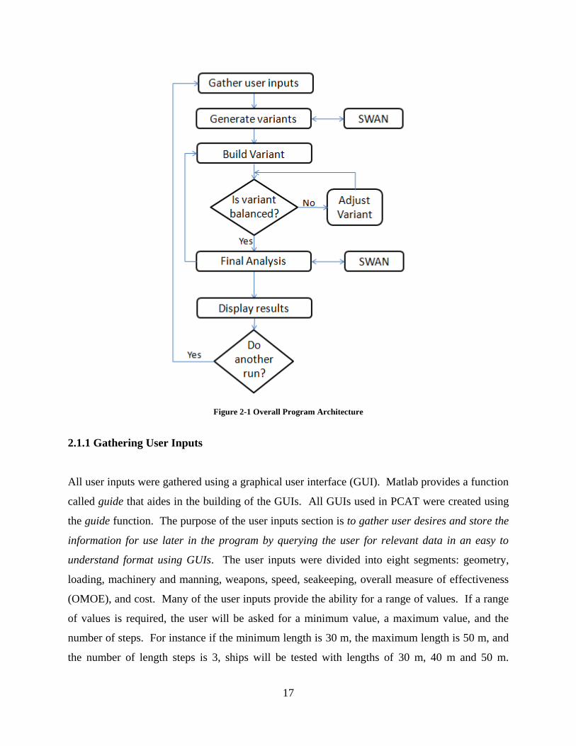
17
Figure 2-1 Overall Program Architecture
2.1.1 Gathering User Inputs
All user inputs were gathered using a graphical user interface (GUI). Matlab provides a function
called guide that aides in the building of the GUIs. All GUIs used in PCAT were created using
the guide function. The purpose of the user inputs section is to gather user desires and store the
information for use later in the program by querying the user for relevant data in an easy to
understand format using GUIs. The user inputs were divided into eight segments: geometry,
loading, machinery and manning, weapons, speed, seakeeping, overall measure of effectiveness
(OMOE), and cost. Many of the user inputs provide the ability for a range of values. If a range
of values is required, the user will be asked for a minimum value, a maximum value, and the
number of steps. For instance if the minimum length is 30 m, the maximum length is 50 m, and
the number of length steps is 3, ships will be tested with lengths of 30 m, 40 m and 50 m.
18
However, the number of steps is ignored is the user desires a response surface model built. Only
the minimum and the maximum values are required.
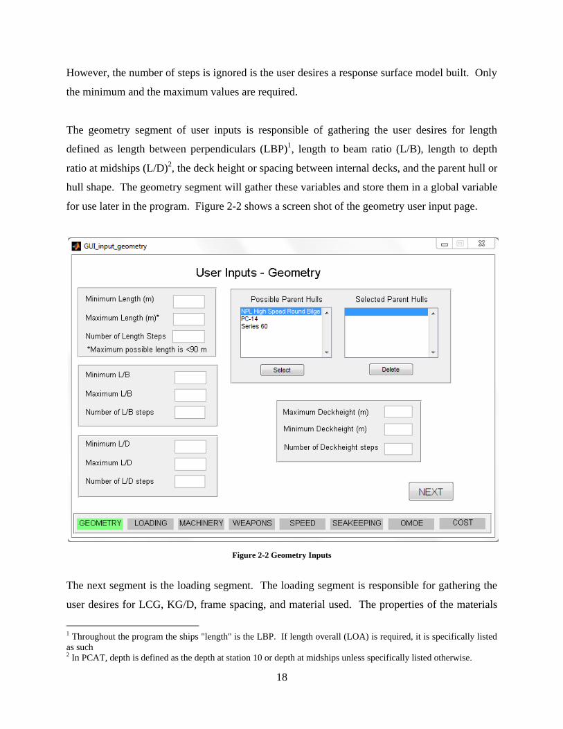
The geometry segment of user inputs is responsible of gathering the user desires for length
defined as length between perpendiculars (LBP)1, length to beam ratio (L/B), length to depth
ratio at midships (L/D)2, the deck height or spacing between internal decks, and the parent hull or
hull shape. The geometry segment will gather these variables and store them in a global variable
for use later in the program. Figure 2-2 shows a screen shot of the geometry user input page.
Figure 2-2 Geometry Inputs
The next segment is the loading segment. The loading segment is responsible for gathering the
user desires for LCG, KG/D, frame spacing, and material used. The properties of the materials
1 Throughout the program the ships "length" is the LBP. If length overall (LOA) is required, it is specifically listed
as such 2 In PCAT, depth is defined as the depth at station 10 or depth at midships unless specifically listed otherwise.
19
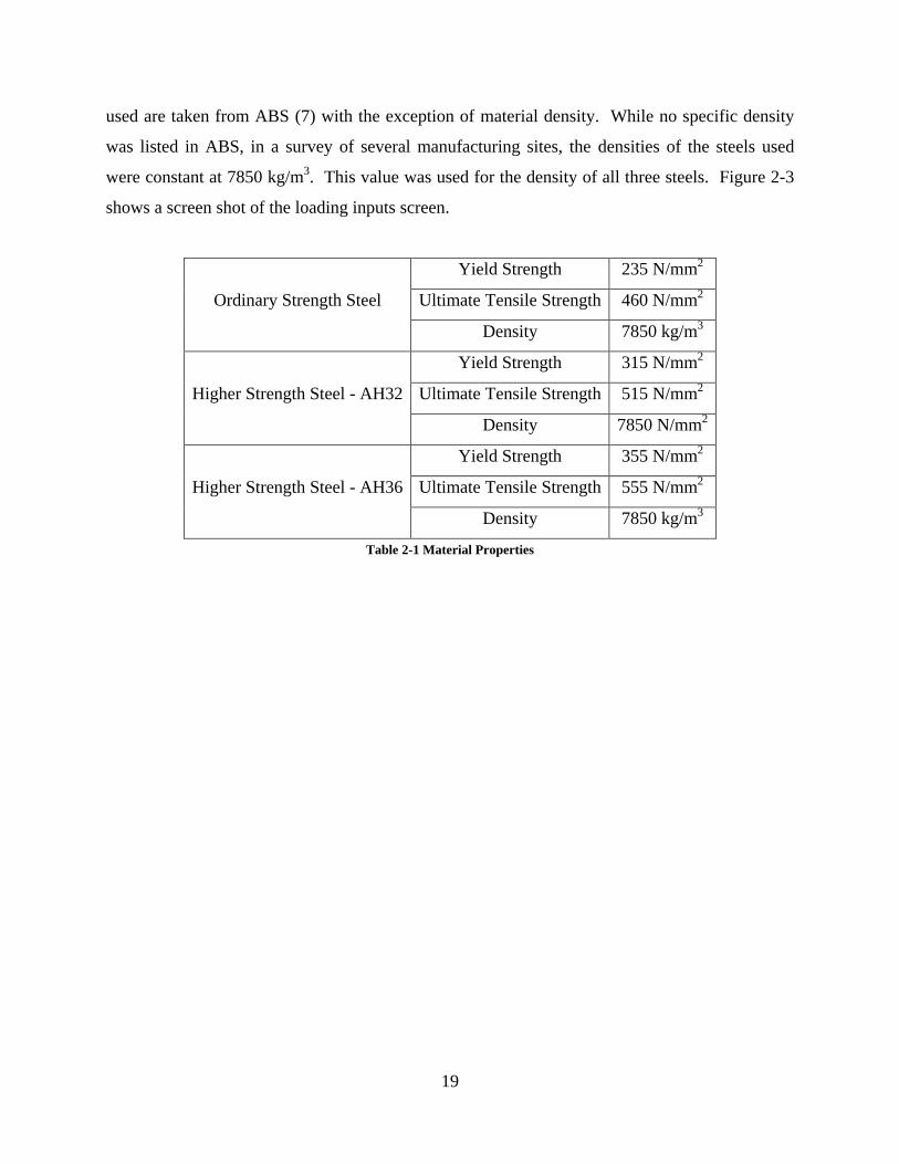
used are taken from ABS (7) with the exception of material density. While no specific density
was listed in ABS, in a survey of several manufacturing sites, the densities of the steels used
were constant at 7850 kg/m3. This value was used for the density of all three steels. Figure 2-3
shows a screen shot of the loading inputs screen.
Ordinary Strength Steel
Yield Strength 235 N/mm2
Ultimate Tensile Strength 460 N/mm2
Density 7850 kg/m3
Higher Strength Steel - AH32
Yield Strength 315 N/mm2
Ultimate Tensile Strength 515 N/mm2
Density 7850 N/mm2
Higher Strength Steel - AH36
Yield Strength 355 N/mm2
Ultimate Tensile Strength 555 N/mm2
Density 7850 kg/m3
Table 2-1 Material Properties

20
Figure 2-3 Loading Inputs
The machinery and manning segment gathers data on the number of engines per shaft, the
number of shafts, and the number and type of manning on board the ship. Additionally this
segment allows the user to specify whether waterjets or propellers will be analyzed used. While
the total value of the ship's crew can be changed over the variants, the breakdown is constant
over all variants. A screen shot of the machinery and manning input screen is shown in Figure
2-4.

21
Figure 2-4 Machinery and Manning Input
Figure 2-5 Weapons Input

22
The weapons segment serves a different function than the other segments. The purpose of the
weapons segment is not to receive a range of weights for weapons but rather to receive a list of
independent sets of weapons, C4I (command, control, communication, computers, and
information), navigation and communication systems to be used on board the ship. Each set of
"weapons" will be used on each variant of ship. For each set, the user enters the total weight,
required in hull area, required main deck or deckhouse area, power requirement, KG/D, measure
of effectiveness for this set of systems (MOE), and cost of this set of systems (the power
requirement and the KG/D currently serve no purpose, but are there as place holders for future
versions of the program). The user must enter all equipment that would normally be part of
SWBS weight groups 400, 700, and variable loads with the exception of fuel loading. This
segment is essentially used to capture mission specific equipment that can be estimated b
traditional means. A screen shot of the weapons input screen is shown in Figure 2-5.
The speed segment gathers information on speed requirements. A speed profile is input to aide
in lifecycle cost calculation. Additionally, maximum speed (or more accurately, the minimum
speed that must be achieved at full power), endurance speed, and range are all gathered in this
segment. A default is provided to set the endurance speed to the most efficient speed. Figure
2-6 shows the speed input screen.

23
Figure 2-6 Speed Input
The seakeeping segment gathers information on the sea keeping environment for analysis. The
sea spectrum used is the Brett Schneider sea spectrum for fully developed seas. This is a two
parameter spectrum that requires the modal frequency and the significant wave height to be
input. Designer’s however, typically define seakeeping requirement in terms of a sea state. The
World Meteorological Organization (WMO) publishes information on sea states (or Beaufort
Scale) (8) including wave heights for a given sea state. Assuming the peak energy of the
spectrum is associated with the mean wave height, the modal frequency can be determined using
the dispersion relationship for deep water waves.
𝜔2 = 𝑔𝑘
The remaining inputs are not currently used, but can be used to determine the sea keeping of a
vessel over an entire operating range of speeds and headings.
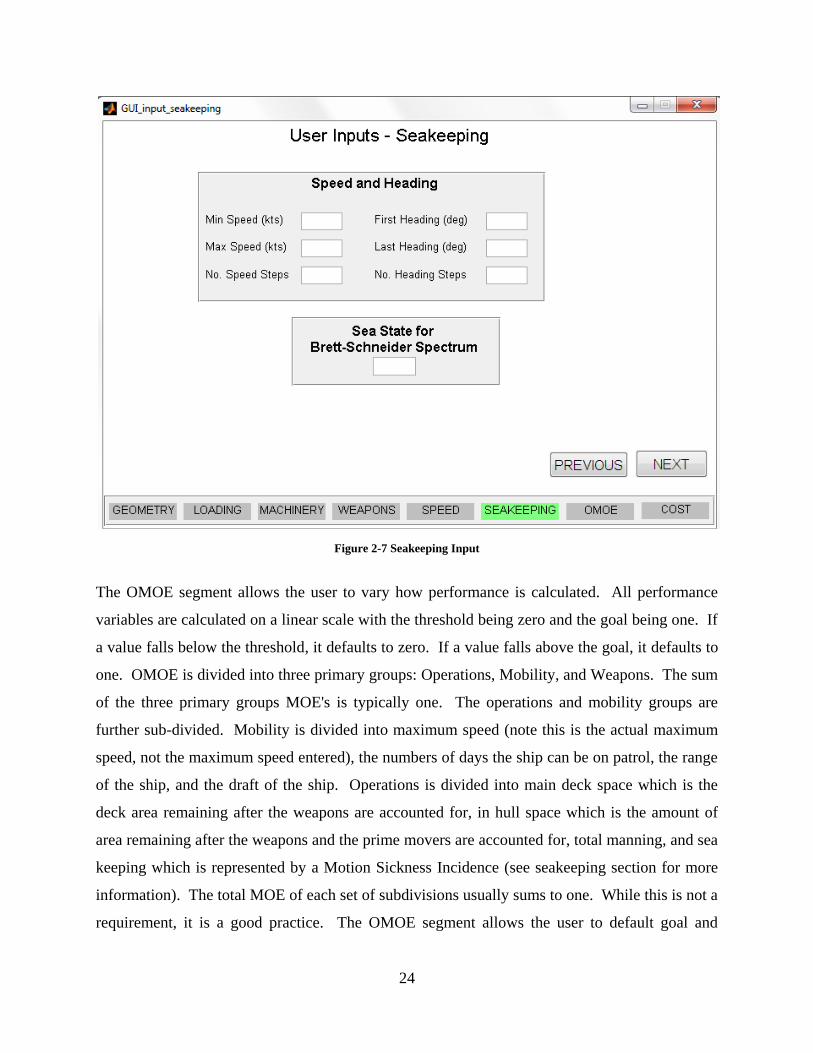
24
Figure 2-7 Seakeeping Input
The OMOE segment allows the user to vary how performance is calculated. All performance
variables are calculated on a linear scale with the threshold being zero and the goal being one. If
a value falls below the threshold, it defaults to zero. If a value falls above the goal, it defaults to
one. OMOE is divided into three primary groups: Operations, Mobility, and Weapons. The sum
of the three primary groups MOE's is typically one. The operations and mobility groups are
further sub-divided. Mobility is divided into maximum speed (note this is the actual maximum
speed, not the maximum speed entered), the numbers of days the ship can be on patrol, the range
of the ship, and the draft of the ship. Operations is divided into main deck space which is the
deck area remaining after the weapons are accounted for, in hull space which is the amount of
area remaining after the weapons and the prime movers are accounted for, total manning, and sea
keeping which is represented by a Motion Sickness Incidence (see seakeeping section for more
information). The total MOE of each set of subdivisions usually sums to one. While this is not a
requirement, it is a good practice. The OMOE segment allows the user to default goal and
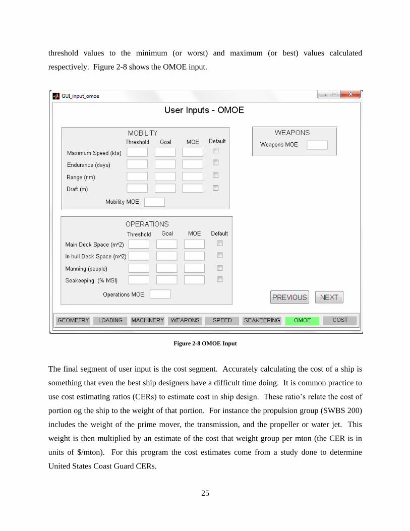
25
threshold values to the minimum (or worst) and maximum (or best) values calculated
respectively. Figure 2-8 shows the OMOE input.
Figure 2-8 OMOE Input
The final segment of user input is the cost segment. Accurately calculating the cost of a ship is
something that even the best ship designers have a difficult time doing. It is common practice to
use cost estimating ratios (CERs) to estimate cost in ship design. These ratio’s relate the cost of
portion og the ship to the weight of that portion. For instance the propulsion group (SWBS 200)
includes the weight of the prime mover, the transmission, and the propeller or water jet. This
weight is then multiplied by an estimate of the cost that weight group per mton (the CER is in
units of $/mton). For this program the cost estimates come from a study done to determine
United States Coast Guard CERs.

26
Life cycle cost encompasses acquisition cost plus the cost of manning and fueling the ship.
There for the designer also inputs the cost of manning in $/man-year, the expected life of the hull
and the percent of time operating the ship is operating, and the cost of fuel. Unlike other
sections, the user is provided with default values because it is not expected that the user will have
fuel cost and manning cost available. The cost function is described in more detail in the next
chapter.
Figure 2-9 Cost Input
2.1.2 Generating Variants
The purpose of the generating variants block is to take the user inputs and generate the set of
hulls that is necessary to explore the user defined design space by assigning parameters to a
particular variant in a variable that can be accessed later.

27
This is accomplished in one of two ways. If the user desires to use a response surface model,
PCAT will ignore the number of steps input by the user and automatically calculate the correct
number of variants to generate using a circumscribed central composite design. If instead the
user desires a full factorial run then, nested loops are used to receive data from the user inputs
block, such as an array of ship lengths, and assign each length to a different variant. The total
number of ships built depends on the number of steps used in the different design variables.
2.1.3 Build Variants
After the design variables are assigned to a ship, the next step is to use that information to design
the ship. The purpose of the building variants block is to take the user inputs of each variant and
construct a model of the ship by systematically adding components to the model. This is done
one variant at a time. The process for building variants is shown in Figure 2-10. Each of the
steps is described in more detail in chapter 3.
The output of the build variants block is either a ship with all its design variables calculated, or a
ship that has failed to complete and has an error message. With all the design variables
calculated, there is one final check: does the weight of the ship equal the displacement? If it
does not, the design waterline is adjusted and the build variant process is restarted at a new draft.
If the displacement and the draft are equal (or nearly equal) then the ship has "converged" and
final analysis can begin.

28
Figure 2-10 Build Variant Process
2.1.4 Final Analysis
After the ship has converged, the final analysis can begin. The final analysis block calculates
seakeeping response, life cycle and acquisition cost, and overall effectiveness while rejecting
ships that converged to an "unbuildable" variant. Examples of unbuildable variants are ships
without adequate internal or external deck space, or ships with a negative metacentric height.
The final analysis section also prepares data for use by the display results block.
2.1.5 Display Results
The last block is not one to be overlooked. If the results are not displayed in a manner that is
useful to the designer, then PCAT is of little practical value. So the display results block seeks to

29
aid the user in determining areas for future study, as well as areas that are fairly well resolved by
showing comparisons of ships both graphically and listing individual ship results.
2.1.6 Completing Another Run
PCAT allows the user to refine and optimize the results an additional "run" of the program. The
results of the first run are not deleted; rather they are kept to allow for comparison with previous
results. The results of both runs are displayed simultaneously to allow the user to determine if the
changes resulted in an improvement in the ship design over previous runs.
2.2 Data Architecture
In a program designed to run many thousands of ship variants with a few hundred parameters per
ship, it is imperative that the data structure be well thought out. Naming of variables must be
clear and apparent to allow for future growth of the program. Additionally, the use of global
variables must be minimized to keep memory free, though there must be maximum flexibility in
the use of variables over numerous functions.
To accomplish these diverse goals, a few key decisions were made. First, there would only be
two global variables: the first holding the user inputs (called USER3), and the second holding the
details of the variants (called HULL). Because there are multiple variants and multiple runs,
HULL is a matrix of variables where each variant is represented by an element of hull. The 1st
dimension of HULL is the variant number while the 2nd
dimension is the run number. For
example HULL(35, 1) refers to the 35th
variant of the first run.
To keep the naming as clear as possible, structures were used. Matlab describes structures as,
"arrays with named data containers' called fields. The fields of a structure can contain any kind
of data. For example, one field might contain a text string representing a name, another might
contain a scalar representing a billing amount, a third might hold a matrix of medical test results,
3 Matlab is a case sensitive code, and in PCAT, HULL and USER are capitalized to bring attention to the global
variables. The rest of the variables and fields are in lowercase. To aide a person in editing the code, all variables
discussed in this thesis are capitalized in the same way as in PCAT.

30
and so on." The use of generic named data containers allows the storage of strings, such as the
name of the parent hull, matrices, and scalars in a single clearly labeled data structure.
For example, the user inputs for the geometry segment are stored in the USER.geometry
structure (note that USER is a structure with field geometry which is also a structure). In this
way it is clear where the array of possible lengths is stored (USER.geometry.length). HULL is
layed out in the same manner. For example HULL(42,2).geometry.depth holds the midships
depth for the 42nd
variant on the 2nd
run. A detailed description of the two global variables is
available in Appendix B.
31
3.0 Module Creation and Validation
With the process laid out, the next step was to create modules that would build a model of the
ship. Each of these modules must be validated to ensure accuracy and then integrated into the
program. While the collection of data from the user is not trivial, there is little to describe in the
creation or validation process that was not discussed in chapter 2. Therefore this chapter begins
with the creation of the variants.
Functions in PCAT are named in a consistent manner to make is easier for a user to improve the
code in the future. To ensure the function names are clear, they are marked with italics in this
paper. The first executable is PCAT, therefore to begin the program the user just types PCAT.
The GUIs are divided into two different sections, the GUIs used for receiving data (input) and
the GUIs used for displaying data (output). All functions that create GUIs are named GUI_input
(or output)_purpose. For instance the GUI that gathers data on the geometry of the ship is
named GUI_input_geometry. PCAT_execute is the "main function" that creates the models of
the hulls. It calls other functions that are named PCAT_purpose. For instance the function that
creates the ship's structure is calculated in PCAT_structures. All of the functions are described
in more detail below.
3.1 Variant Creation
To create a full factorial set of experiments4, the total number of possible ships is calculated.
The user is permitted to allow 15 different variables to take multiple levels: LBP, L/B, L/D, deck
height, the parent hull, KG/D, LCG/L, the material used, frame spacing, the use of water jets or
propellers, the number of engines per shaft, the number of shafts, the number of weapon groups,
range, and total manning. The number of levels of each of these variables (the length of each
array) is multiplied together to get the total number of ships to create. The number of possible
ship types can grow very quickly with 15 different variables. Even if each variable only takes on
2 possible values, the total number of possible ships will still be 215
or 32,768. Therefore it is
necessary for the user to have a rough idea of the boundaries of the design space before
4 For information on a reduced set of experiments and response surface modeling see chapter 4.
32
beginning, though functionality was added to aid the user in narrowing the design space while
adding granularity to the possible designs through the use of multiple runs.
With the total number of designs known, PCAT then assigns design variables to each variant.
This is done with nested loops running over each of the design variables listed above.
Once the hull parameters are set, the shape of an individual hull will not be changed throughout
the program. Therefore, PCAT scales the parent hull before any computations begin. The
scaling is done a function called PCAT_scale. There are four dimensions that need to be scaled,
the longitudinal offsets, the transverse offsets, the depth offsets, and the initial draft of the hull.
The transverse and longitudinal offsets are scaled in the following manner (it is important to note
that the functions below are not exact Matlab code in PCAT, but rather just show the process
used):
offsets.X = desired_lbp * Xo / max(Xo)
offsets.Y = desired_beam/2 * Y0 / max(Yo)
where Xo and Yo are the original X and Y offsets and offsets.X and offsets.Y are the final offsets.
The beam is divided by two because the offsets used in PCAT are half breadths.
Scaling the ships depth is slightly more complicated because it is likely that the ships depth is not
maximum at the midsection. To account for this, the depth of the parent hull at midships must be
determined. The first step is finding the index of the midsection in the longitudinal array
(offsets.X). Then, at the ship's midsection, the index of the highest half breadth is found.
[temp, mid]=min(abs(X – LBPo/2)) %mid is the index of the midsection
for n=length(Z):-1:1
if ~isnan(Y(mid, n) %this will break when the half breadth exists
break %hence n is the index of the max depth at midships
end %and Z(n) is the maximum depth
end
33
Z = input.depth * Zo / Z(n) %Zo is the original Z offsets
t = input.depth * to / Z(n)
This process is spelled out in detail because it arises many times throughout the course of PCAT.
The assignment function and the scaling function were validated by inspection. All of this
functionality is done in first half of the function PCAT_execute.
3.1.1 Possible Parent Hulls
Three parent hulls were loaded into PCAT, the PC-14 hull, the NPL High Speed Round Bilge
Hull, and the Series 60 hull form. The NPL High Speed Round Bilge hull was designed for
operation in the Froude number (FN) range of 0.3 – 1.2. According to Bailey, this hull could be
used as a heavily loaded work boat, a fast patrol craft, or a small naval ship. The round bilge of
the hull form allows for lower resistance than a flat bottomed planing hull in the semi-
displacement region, while still providing more lifting than a typical surface combatant hull. The
offsets for the NPL Hull were obtained directly from Bailey's work with the hull (9).
The primary mission of the PC is coastal patrol and interdiction surveillance. These ships also
provide full mission support for Navy SEALs and other special operations forces. The PC ships,
also known as the cyclone class, provide the U.S. Navy with a fast, reliable platform that can
respond to emergent requirements in a low intensity conflict environment(10). The offsets for
the PC-14 were taken from a converged ASSET model of the PC-14 created by the U.S. Navy
(11).
The Series-60 hull form is a typical merchant hull form. While not ideal for high speed semi
displacement craft, the hull offsets were added to allow for an additional hull form for
comparison.
Additional parent hulls can be easily inserted into PCAT in the PCAT_offsets file. However, the
user must also be able to model the hull interaction with the propulsion system to account for
34
changes in resistance and powering due to changing flow around the hull. More information on
this topic can be found in the shaft horse power section below.
3.2 Variant Geometry
With the variant hull defined, the next step is to determine the applicable geometric parameters
for use in other modules later in the program. All geometric parameters were determined using
techniques described in Principles of Naval Architecture (12) and Introduction to Naval
Architecture (13).
Most of the geometrical parameters apply only to the immersed section of the hull, so the first
step is to insert interpolated offsets at the current waterline and shorten the waterline array (Z)
and the half breadth array (Y) to include offsets only below the water line.
With no bounds on the spacing of the offsets, it would not be wise to attempt to use Simpson's
multipliers to integrate sections and areas. Simpson's technique assumes a quadratic shape to
find areas. However, for an arbitrary spacing of the offsets, this would be difficult. Therefore
the trapezoidal rule was used for integration and interpolation. The trapezoidal rule assumes a
linear shape for integration. This allows the offsets to be entered in whatever spacing is
available to the user. The trapezoidal rule is used extensively throughout PCAT.
First the section areas are calculated.
𝑆𝑒𝑐𝑡𝑖𝑜𝑛 𝑎𝑟𝑒𝑎 𝑥 = 2 ∗ 𝐻𝑎𝑙𝑓 𝑏𝑟𝑒𝑎𝑑𝑡 𝑥, 𝑧 𝑑𝑧
𝑤𝑎𝑡𝑒𝑟𝑙𝑖𝑛𝑒
𝑏𝑎𝑠𝑒𝑙𝑖𝑛𝑒
The displaced volume (∇) is calculated by integrating the section areas.
∇ = 𝑆𝑒𝑐𝑡𝑖𝑜𝑛 𝐴𝑟𝑒𝑎 𝑥 𝑑𝑥
𝑙𝑒𝑛𝑔𝑡
35
The displacement (Δ) is then is calculated using a density of sea water (1025 kg/m3)
∆= ∇ ∗ 𝜌
The longitudinal center of buoyancy (LCB) was calculated by integrating the moment of the
section areas.
𝐿𝐶𝐵 = 𝑥 ∗ 𝑆𝑒𝑐𝑡𝑖𝑜𝑛 𝐴𝑟𝑒𝑎 𝑥 𝑑𝑥𝑙𝑒𝑛𝑔𝑡
∇
The beam at the water line is simply twice the maximum half breath of the immersed section.
The block coefficient (Cb) and prismatic coefficient (Cp) are also calculated.
𝐶𝑏 =∇
𝐿𝐵𝑃 ∗ 𝑑𝑟𝑎𝑓𝑡 ∗ 𝑏𝑒𝑎𝑚 𝑎𝑡 𝑤𝑎𝑡𝑒𝑟𝑙𝑖𝑛𝑒
𝐶𝑝 =∇
𝐿𝐵𝑃 ∗ 𝑚𝑎𝑥𝑖𝑚𝑢𝑚 𝑠𝑢𝑏𝑚𝑒𝑟𝑔𝑒𝑑 𝑠𝑒𝑐𝑡𝑖𝑜𝑛 𝑎𝑟𝑒𝑎
The metacentric height (GM) is an excellent measure of initial static stability. GM is defined as
the difference between the height of the metacenter (KM) and the height of the center of gravity
above the keel (KG). KM can be defined as the height of the center of buoyancy above the keel
(KB) plus the height of the metacenter above the center of buoyancy (BM).
𝐼𝑡𝑟𝑎𝑛𝑠𝑣𝑒𝑟𝑠𝑒 =2
3 𝑦 𝑥
3
𝑙𝑒𝑛𝑔𝑡
𝑑𝑥
𝐵𝑀 =𝐼𝑡𝑟𝑎𝑛𝑠𝑣𝑒𝑟𝑠𝑒
∇
To find KB, the moment of areas of the water planes are integrated and divided by the volume.
36
𝑤𝑎𝑡𝑒𝑟𝑝𝑙𝑎𝑛𝑒 𝑎𝑟𝑒𝑎 𝑧 = 2 𝑦 𝑥, 𝑧 𝑑𝑥
𝑙𝑒𝑛𝑔𝑡
𝐾𝐵 =1
∇ 𝑧 ∗ 𝑤𝑎𝑡𝑒𝑟𝑝𝑙𝑎𝑛𝑒 𝑎𝑟𝑒𝑎 𝑧 𝑑𝑧
𝑤𝑎𝑡𝑒𝑟𝑙𝑖𝑛𝑒
𝑏𝑎𝑠𝑒𝑙𝑖𝑛𝑒
𝐺𝑀 = 𝐾𝐵 + 𝐵𝑀− 𝐾𝐺
The wetted surface area (WSA) is the final variable calculated using the immersed offsets. The
WSA is calculated by integrating the length of curves around the hull at a given longitudinal
location.
𝑙𝑒𝑛𝑔𝑡 𝑜𝑓 𝑐𝑢𝑟𝑣𝑒 𝑥 = (𝑦 𝑥,𝑛 − 𝑦 𝑥,𝑛 − 1 )2 + (𝑧 𝑛 − 𝑧 𝑛 − 1 )2
𝑙𝑒𝑛𝑔𝑡 (𝑧)
𝑛=1
𝑊𝑆𝐴 = 𝑙𝑒𝑛𝑔𝑡 𝑜𝑓 𝑐𝑢𝑟𝑣𝑒 𝑥 𝑑𝑥
𝑙𝑒𝑛𝑔𝑡
The deck area calculations are also calculated in the geometry sections. The main deck area is
calculated as the area of the surface that connects the highest offsets at every station. The user
specifies the internal decks spacing (dh). The first internal deck is place dh feet below height of
the main deck at midships. All internal decks are parallel with the base line.
𝑚𝑎𝑖𝑛 𝑑𝑒𝑐𝑘 𝑎𝑟𝑒𝑎 = 1
2 𝑦 𝑛, 𝑧𝑜 + 𝑦 𝑛 + 1, 𝑧1 ∗ 𝑥 𝑛 + 1 − 𝑥 𝑛
2+ (𝑧(𝑧1) − 𝑧(𝑧𝑜))2
𝑙𝑒𝑛𝑔𝑡 (𝑥)
𝑛=1
Where zo is the maximum height at longitudinal point n, and z1 is the maximum height at the
next longitudinal point.
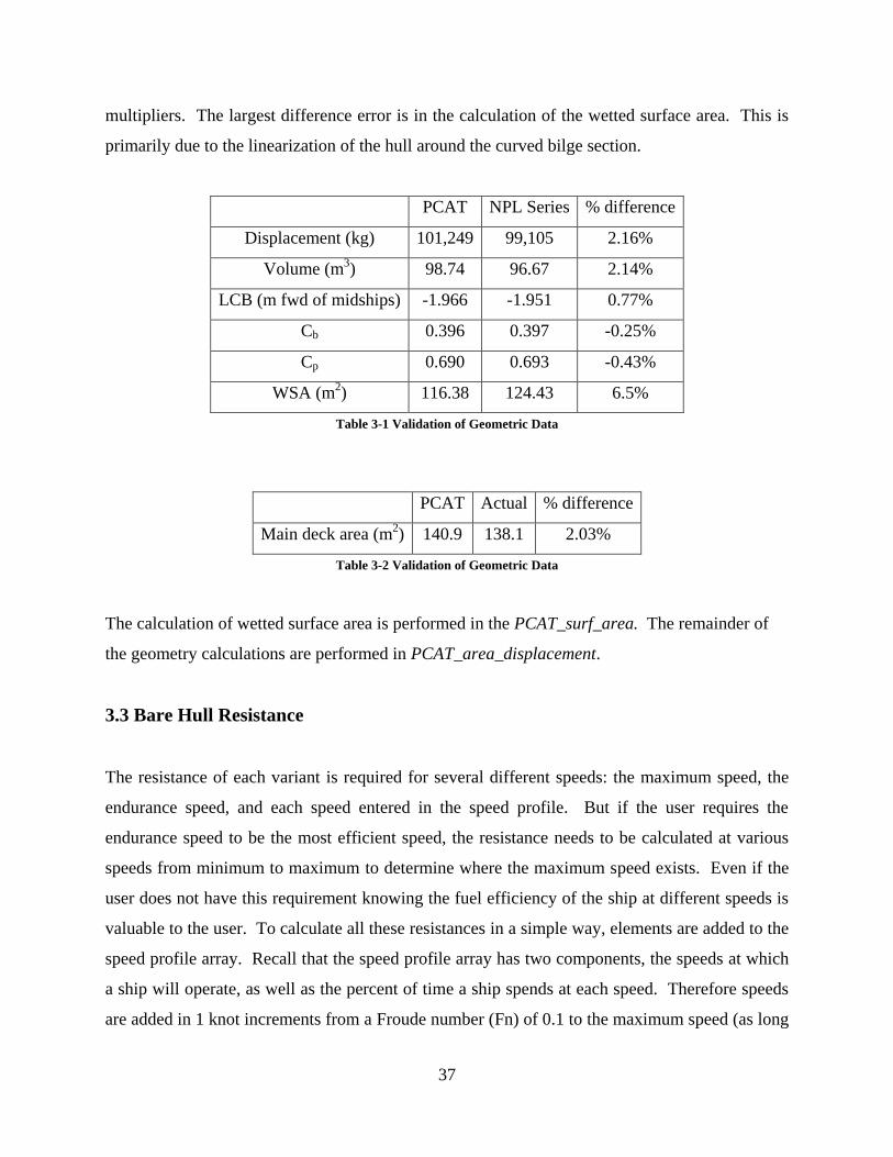
To validate the geometry code, PCAT was run with only a 30.5 m NPL series hull loaded. The
actual values in Table 3-1 were gathered directly from the NPL series (9), while the actual values
in Table 3-2 were calculated by hand using a quadratic approximation using Simpson's
37
multipliers. The largest difference error is in the calculation of the wetted surface area. This is
primarily due to the linearization of the hull around the curved bilge section.
PCAT NPL Series % difference
Displacement (kg) 101,249 99,105 2.16%
Volume (m3) 98.74 96.67 2.14%
LCB (m fwd of midships) -1.966 -1.951 0.77%
Cb 0.396 0.397 -0.25%
Cp 0.690 0.693 -0.43%
WSA (m2) 116.38 124.43 6.5%
Table 3-1 Validation of Geometric Data
PCAT Actual % difference
Main deck area (m2) 140.9 138.1 2.03%
Table 3-2 Validation of Geometric Data
The calculation of wetted surface area is performed in the PCAT_surf_area. The remainder of
the geometry calculations are performed in PCAT_area_displacement.
3.3 Bare Hull Resistance
The resistance of each variant is required for several different speeds: the maximum speed, the
endurance speed, and each speed entered in the speed profile. But if the user requires the
endurance speed to be the most efficient speed, the resistance needs to be calculated at various
speeds from minimum to maximum to determine where the maximum speed exists. Even if the
user does not have this requirement knowing the fuel efficiency of the ship at different speeds is
valuable to the user. To calculate all these resistances in a simple way, elements are added to the
speed profile array. Recall that the speed profile array has two components, the speeds at which
a ship will operate, as well as the percent of time a ship spends at each speed. Therefore speeds
are added in 1 knot increments from a Froude number (Fn) of 0.1 to the maximum speed (as long

38
as the maximum speed has a Fn < 1.0). For every element that is added to the speed array, a 0 is
added to the percentage array in the same location. This represents the ship spending 0% of its
time at any new speed added. This process occurs in PCAT_beefup.
Froude hypothesized that resistance could be broken down into two basic areas. Frictional
resistance which is a function of Reynolds number, and residual resistance which encompasses
all other resistance terms, primarily wave making resistance and form drag. The frictional
resistance coefficient is calculated using the standard 1957 International Towing Tank
Convention (ITTC) formula.
𝐶𝑓 =0.075
𝑙𝑜𝑔10𝑅𝑁 − 2 2
Where the total frictional resistance is:
𝐷𝑓 =1
2𝜌𝑆𝑈2(𝐶𝑓 + 𝐶𝑎)
Where S is the wetted surface area in m2, U is the ships speed in m/s, ρ is the density of water in
kg/m3, and Ca is the correlation allowance. The correlation allowance is set at 0.0004.
Calculation of the residual resistance can be done using several methods. The most accurate
method is to build a model and test the hull; however that is impractical for this project. A
discussion of possible methods for calculating residual resistance for patrol crafts follows
(14)(15).
Canadian Research Council – Fast Surface Ship – This method is used to calculate residual
resistance for ships operating in the displacement region. High speed slender ships that operate
at Froude number below 0.83 are a good fit for this method. This method is based on regression
analysis of model test data.

39
Hamburg Ship Model Basin – This method uses Telfer type regression of model data to predict
residual resistance for small higher speed ships. This method is good for ships operating up to
Froude numbers of 0.83.
Semi Displacement Double Chine – This method is based on regression data performed by the
National Technical University of Athens on double chine, transom stern, semi displacement hull
series. This series is intended for large high speed vehicles operating below Froude numbers of
0.53.
Semiplaning Transom Stern - This method is designed for the ships in the displacement and
semi-displacement region for Froude numbers up to 0.53. Regression analysis was performed at
the U.S. Naval Academy Hydrodynamics Laboratory on various hulls.
Compton – This algorithm is designed for typical coastal patrol, training, or recreational
powerboat hull forms with transom sterns operating in the displacement or semi displacement
regions. This resistance method is good for Froude numbers from 0.1 to 0.6 (16).
While all of these methods can provide a good estimate for bare hull resistance, they are all
parametrically derived and can have difficulty differentiating subtle differences in hull types.
Finding a method of calculating resistance accurately from the zero speed (displacement only)
through a Fn of 1.0 (semi-displacement) is difficult because of the differences in dynamic
support the vessel receives. Additionally, each method has its own set of restrictions where it is
valid. The restrictions for the Compton method are shown below as an example.
Lower Limit Upper Limit
Speed (kts)/√LWL 0.35 2.00
𝐹𝑁∇ 0.3 1.5
∆(0.01 ∗ 𝐿𝐵𝑃)3 105 150
LCG/LBP -0.13 -0.02
LBP/B 4.0 5.2
Table 3-3 Compton Resistance Bounds

40
To allow the user the widest range of possible inputs and to aide in capturing all differences in
hull shape, size, and weight distribution, SWAN2 was used to generate the residual resistance.
Being a potential flow model, SWAN2 can accurately provide the resistance generated by the
waves, however, SWAN2 cannot derive the form resistance for high speed vessels with transom
sterns. Form resistance is highly dependent on the flow separation that occurs at the transom of
high speed ships. Because SWAN2 is a potential flow program, it cannot simulate this effect.
However, at high Fn (0.5-1.0), the form drag has been shown to be independent of speed and
approximately half the frictional drag (17). So the residual resistance coefficient is calculated as
follows.
𝐶𝑟 = 𝐶𝑤 +1
2𝐶𝑓
Where Cw is the wave resistance coefficient provided by SWAN2.
The total resistance (DT) and bare hull horse power (EHP) are calculated as follows.
𝐶𝑇 = 𝐶𝑓 + 𝐶𝑎 + 𝐶𝑟
𝐷𝑇 =1
2𝜌𝑆𝑈2(𝐶𝑇)
𝐸𝐻𝑃𝐵𝐻 𝑈 = 𝑈 ∗ 𝐷𝑇(𝑈)
Where S is the wetted surface area in m2, U is the ships speed in m/s, and ρ is the density of
water in kg/m3. To validate the resistance subroutine, two methods were used. First the results
were compared to results of the same ships using Compton method. Additionally, the results
were compared to Maxsurf's Hull Speed module which has the ability to calculate residual
resistance. The hull used was a 33 ft YP, the same hull used by Roger Compton in his initial
study (16).

41
Figure 3-1 Accuracy of PCAT Resistance
The results from this routine were very pleasing. SWAN2 residual resistance provides an
accurate measure of resistance, within 10% throughout the design range.
The interface with an external program like SWAN2 is difficult. It requires meticulous coding to
ensure all inputs and outputs are in the correct format and can be exchanged between the
programs seamlessly. To interface with SWAN2 is a multi-step process. The first step is
ensuring that the offsets are formatted correctly for SWAN2. In SWAN2 the offsets are written
into a text file with a .pln extension. Therefore PCAT_writepln scales the offsets and writes the
offsets to the correct format for use in SWAN2.
Next, SWAN2 requires a file to input the job control parameters, a .inp or input file. This file
describes the analysis that is required and provides further details about the ship. Information
included in the .inp file include: ship length, depth, speed, mass, and radii of gyration as well as
water density and information required to set up the free surface boundary and mesh grid. The
4 6 8 10 12 14 16 18 200
200
400
600
800
1000
1200
1400
1600
Speed (kts)
Bare
Hull
Resis
tance (
kW
)
PCAT Accuracy
PCAT (using SWAN)
Compton
MaxSurf
42
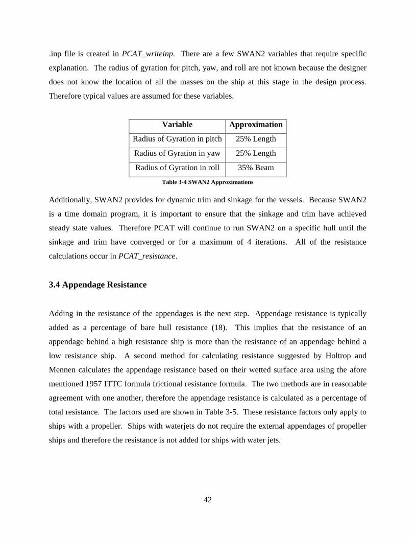
.inp file is created in PCAT_writeinp. There are a few SWAN2 variables that require specific
explanation. The radius of gyration for pitch, yaw, and roll are not known because the designer
does not know the location of all the masses on the ship at this stage in the design process.
Therefore typical values are assumed for these variables.
Variable Approximation
Radius of Gyration in pitch 25% Length
Radius of Gyration in yaw 25% Length
Radius of Gyration in roll 35% Beam
Table 3-4 SWAN2 Approximations
Additionally, SWAN2 provides for dynamic trim and sinkage for the vessels. Because SWAN2
is a time domain program, it is important to ensure that the sinkage and trim have achieved
steady state values. Therefore PCAT will continue to run SWAN2 on a specific hull until the
sinkage and trim have converged or for a maximum of 4 iterations. All of the resistance
calculations occur in PCAT_resistance.
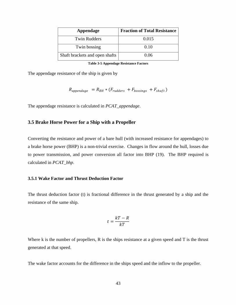
3.4 Appendage Resistance
Adding in the resistance of the appendages is the next step. Appendage resistance is typically
added as a percentage of bare hull resistance (18). This implies that the resistance of an
appendage behind a high resistance ship is more than the resistance of an appendage behind a
low resistance ship. A second method for calculating resistance suggested by Holtrop and
Mennen calculates the appendage resistance based on their wetted surface area using the afore
mentioned 1957 ITTC formula frictional resistance formula. The two methods are in reasonable
agreement with one another, therefore the appendage resistance is calculated as a percentage of
total resistance. The factors used are shown in Table 3-5. These resistance factors only apply to
ships with a propeller. Ships with waterjets do not require the external appendages of propeller
ships and therefore the resistance is not added for ships with water jets.
43
Appendage Fraction of Total Resistance
Twin Rudders 0.015
Twin bossing 0.10
Shaft brackets and open shafts 0.06
Table 3-5 Appendage Resistance Factors
The appendage resistance of the ship is given by
𝑅𝑎𝑝𝑝𝑒𝑛𝑑𝑎𝑔𝑒 = 𝑅𝐵𝐻 ∗ (𝐹𝑟𝑢𝑑𝑑𝑒𝑟𝑠 + 𝐹𝑏𝑜𝑠𝑠𝑖𝑛𝑔𝑠 + 𝐹𝑠𝑎𝑓𝑡 )
The appendage resistance is calculated in PCAT_appendage.
3.5 Brake Horse Power for a Ship with a Propeller
Converting the resistance and power of a bare hull (with increased resistance for appendages) to
a brake horse power (BHP) is a non-trivial exercise. Changes in flow around the hull, losses due
to power transmission, and power conversion all factor into BHP (19). The BHP required is
calculated in PCAT_bhp.
3.5.1 Wake Factor and Thrust Deduction Factor
The thrust deduction factor (t) is fractional difference in the thrust generated by a ship and the
resistance of the same ship.
𝑡 =𝑘𝑇 − 𝑅
𝑘𝑇
Where k is the number of propellers, R is the ships resistance at a given speed and T is the thrust
generated at that speed.
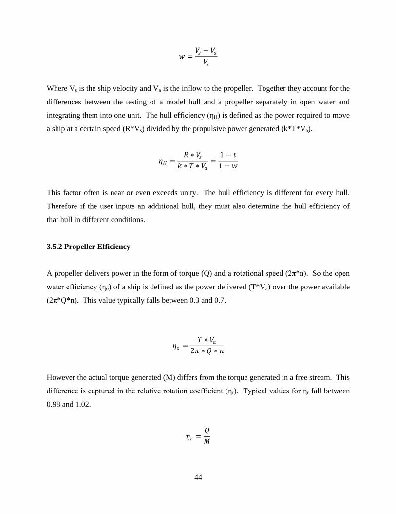
The wake factor accounts for the difference in the ships speed and the inflow to the propeller.
44
𝑤 =𝑉𝑠 − 𝑉𝑎
𝑉𝑠
Where Vs is the ship velocity and Va is the inflow to the propeller. Together they account for the
differences between the testing of a model hull and a propeller separately in open water and
integrating them into one unit. The hull efficiency (ηH) is defined as the power required to move
a ship at a certain speed (R*Vs) divided by the propulsive power generated (k*T*Va).
𝜂𝐻 =𝑅 ∗ 𝑉𝑠
𝑘 ∗ 𝑇 ∗ 𝑉𝑎=
1 − 𝑡
1 −𝑤
This factor often is near or even exceeds unity. The hull efficiency is different for every hull.
Therefore if the user inputs an additional hull, they must also determine the hull efficiency of
that hull in different conditions.
3.5.2 Propeller Efficiency
A propeller delivers power in the form of torque (Q) and a rotational speed (2π*n). So the open
water efficiency (ηo) of a ship is defined as the power delivered (T*Va) over the power available
(2π*Q*n). This value typically falls between 0.3 and 0.7.
𝜂𝑜 =𝑇 ∗ 𝑉𝑎
2𝜋 ∗ 𝑄 ∗ 𝑛
However the actual torque generated (M) differs from the torque generated in a free stream. This
difference is captured in the relative rotation coefficient (ηr). Typical values for ηr fall between
0.98 and 1.02.
𝜂𝑟 =𝑄
𝑀
45
3.5.3 Efficiencies for Given Hulls
The wake factor and thrust deduction factor for the PC hull were taken from the ASSET values.
Both are assigned values of 0. The relative rotation coefficient is also taken from the ASSET
model of the PC and is assigned a value of 1. The open water efficiency of the propeller is
assigned a value of 0.65 based on Woud and Stapersma (19).
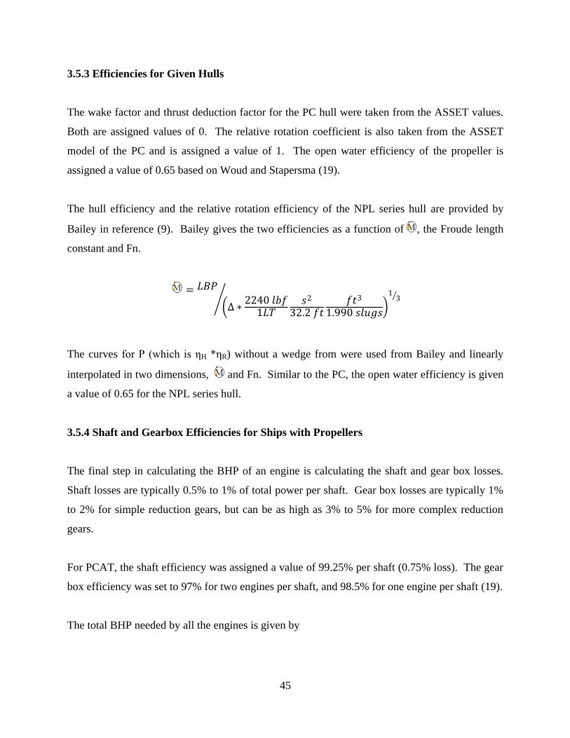
The hull efficiency and the relative rotation efficiency of the NPL series hull are provided by
Bailey in reference (9). Bailey gives the two efficiencies as a function of , the Froude length
constant and Fn.
= 𝐿𝐵𝑃
Δ ∗2240 𝑙𝑏𝑓
1𝐿𝑇𝑠2
32.2 𝑓𝑡𝑓𝑡3
1.990 𝑠𝑙𝑢𝑔𝑠
13
The curves for P (which is ηH *ηR) without a wedge from were used from Bailey and linearly
interpolated in two dimensions, and Fn. Similar to the PC, the open water efficiency is given
a value of 0.65 for the NPL series hull.
3.5.4 Shaft and Gearbox Efficiencies for Ships with Propellers
The final step in calculating the BHP of an engine is calculating the shaft and gear box losses.
Shaft losses are typically 0.5% to 1% of total power per shaft. Gear box losses are typically 1%
to 2% for simple reduction gears, but can be as high as 3% to 5% for more complex reduction
gears.
For PCAT, the shaft efficiency was assigned a value of 99.25% per shaft (0.75% loss). The gear
box efficiency was set to 97% for two engines per shaft, and 98.5% for one engine per shaft (19).
The total BHP needed by all the engines is given by

46
𝐵𝐻𝑃 =𝐸𝐻𝑃
𝜂𝐻𝜂𝑟𝜂𝑜𝜂𝑠𝑎𝑓𝑡 𝜂𝐺𝐵
3.6 Brake Horse Power for a Ships with a Waterjet
Calculating the overall propulsive coefficient of a ship powered by water jet engines is inherently
different than propeller ships. Because the impeller of the water jet exists inside the ship and not
in the turbulent area external to the ship terms such as wake fraction have no meaning.
Additionally, the relative rotation coefficient and the open water efficiency do not correlate to
physical terms in a ship powered by water jets (20).
The water entering the waterjet is accelerated and exerts a momentum drag on the ship. So the
net thrust generated (TN) can be given by
𝑇𝑁 = 𝑇𝐺 − 𝐷𝑀 = 𝑚 𝑗𝑉𝑗 −𝑚 𝑖𝑉𝑠
Where TG is the thrust generated, DM is the momentum drag, 𝑚 𝑗 is the mass flow rate out of the
jet, Vj is the velocity at the outlet of the jet, 𝑚 𝑖 is the mass flow rate to the inlet of the jet, and VS
is ship speed. Unless some flow is bled off the inlet of the water jet, 𝑚 𝑖 = 𝑚 𝑗 . This simplifies
the net thrust to
𝑇𝑁 = 𝑚 𝑉𝑗 − 𝑉𝑠
The work done propelling the ship is then
𝑊𝑁 = 𝑇𝑁𝑉𝑠 = 𝑚 𝑉𝑠 𝑉𝑗 − 𝑉𝑠
To calculate the energy lost in the jet it is necessary to assume that the potential energy gained in
the elevation of the water is negligible and assume perfect inlet energy recovery. Then the
energy added by the pump is the difference in the kinetic energy of the inlet and the outlet of the
water jet.

47
∆𝐾𝐸 =1
2𝑚 𝑗𝑉𝑗
2 −1
2𝑚 𝑖𝑉𝑠
2
Again, assuming the flow rates are equal,
∆𝐾𝐸 =1
2𝑚 𝑉𝑗
2 − 𝑉𝑠2
The efficiency of the jet (ηj) is then given by the ratio of useful work done on the ship to useful
work done by the jet.
𝜂𝑗 =𝑊𝑁
∆𝐾𝐸=
𝑚 𝑉𝑠 𝑉𝑗 − 𝑉𝑠
12𝑚 𝑉𝑗
2 − 𝑉𝑠2
=2𝑉𝑠
𝑉𝑗 + 𝑉𝑠
If a new term µ, is defined as Vs/Vj, then the jet efficiency can be represented as follows.
𝜂𝑗 =2𝜇
1 + 𝜇
However, if a loss coefficient, ζ, is included which represents the total energy lost an a
proportion of the ideal inlet energy, then the energy added by the pump is written,
∆𝐾𝐸 =1
2𝑚 𝑉𝑗
2 − 𝑉𝑠2 + ζ
1
2𝑚 𝑉𝑠
2
∆𝐾𝐸 =1
2𝑚 𝑉𝑗
2 − 𝑉𝑠2 1 − ζ
This changes the jet efficiency to
𝜂𝑗 =2𝜇 1 − 𝜇
1 − 𝜇2 1 − 𝜁
48
This is the definition of jet efficiency that PCAT uses. In a well designed system, ζ can range
from 0.25 to 0.50. In a poorly designed system, ζ can range from 0.5 to 1.0 (20). For
consistency, it is assumed that all ships with water jets have a loss coefficient of 0.5.
So the efficiency of the waterjet is now a function of only ships speed and the waterjet outlet
velocity.
The quazi propulsive coefficient (QPC) for water jets is then equal to,
𝑄𝑃𝐶 = 𝜂𝑗𝜂𝑝
where 𝜂𝑝 is the efficiency of the pump5. The QPC is nominally 0.53 for ships in PCAT’s range
(20). Ships with waterjets do not normally require gearboxes, therefore there is no need for a
gearbox efficiency, and there is no shaft, so there are no shaft losses. So the total power needed
by the engines (BHP) is,
𝐵𝐻𝑃 =𝐸𝐻𝑃
𝑄𝑃𝐶
This calculated in PCAT_bhpwj.
3.7 Engine Selection
With the total load known for the engines, the engines can be selected. To simplify the selection
process, it is assumed that all propulsion engines onboard the ship will be the same type. In
reality it is likely that if there are two engines per shaft, one will be a cruise engine, and the
second, a larger engine to achieve maximum speed. However, most ships of this size analyzed
by PCAT only have one engine per shaft, so the simplification does not have that large an
impact.
5 The QPC for a ship with a propeller is 𝜂𝐻𝜂𝑟𝜂𝑜 .
49
The smallest engine is selected from the engine library that meets the propulsion requirements of
the ship. The engine library is contained in Appendix C.
3.8 Fuel Loading and Efficiency
With the engines selected and the resistance profile known, the total amount of fuel needed to
reach a certain range can be calculated as well as the fuel efficiency at all the speeds.
To do this the engines on board the ship are loaded in one knot increments. Starting from the
lowest speed, one engine is brought on line. When the BHP required to meet a new speed
exceeds the power available of a single engine, an engine from another shaft is brought online.
This continues until there is one engine on each shaft. If more than one engine exists per shaft,
then the pairs of engines are brought online on each shaft next until the required BHP is met.
This continues until the maximum speed is achieved.
At each speed the fuel consumption of the propulsion engines is calculated using the SFC.
𝑃𝑟𝑜𝑝𝑢𝑙𝑠𝑖𝑜𝑛 𝐹𝑢𝑒𝑙 𝐶𝑜𝑛𝑠𝑢𝑚𝑝𝑡𝑖𝑜𝑛 𝑅𝑎𝑡𝑒 𝑘𝑔
𝑟
= 𝑆𝐹𝐶 𝑎𝑡 𝑔𝑖𝑣𝑒𝑛 𝑅𝑃𝑀 𝑘𝑔
𝑘𝑊 − 𝑟 ∗ 𝐵𝐻𝑃(𝑎𝑡 𝑠𝑎𝑚𝑒 𝑅𝑃𝑀)(𝑘𝑊)
In this way the propulsion fuel consumption rate is a function of speed. However there is
another component of fuel efficiency, the fuel used to power the electrical system. Because the
calculation of the total power load is difficult when many of the systems remain undefined, all
variants are assigned the same electrical generators; two Caterpillar 3412 diesel generators
providing 400kW each. It is assumed that each variant can cruise on 400kW, the second
generator is provided for battle conditions and as a spare for cruising. The electrical generator
uses 123.0 liters per hour (lph) (21) when at full load. Assuming a density of fuel of 0.88 kg/L,
the electrical generator uses 24.5 kg/hr of fuel.

50
To get the total fuel efficiency the propulsion fuel consumption rate is added to the electrical fuel
consumption rate to get the total fuel consumption rate. Note that the fuel efficiency and the fuel
consumption rate are both functions of speed.
𝐹𝑢𝑒𝑙 𝐸𝑓𝑓𝑖𝑐𝑖𝑒𝑛𝑐𝑦 𝑛𝑚
𝑚𝑡𝑜𝑛 =
1000 𝑘𝑔
𝑚𝑡𝑜𝑛
1
𝐹𝑢𝑒𝑙 𝐶𝑜𝑛𝑠𝑝𝑢𝑚𝑡𝑖𝑜𝑛 𝑅𝑎𝑡𝑒 𝑘𝑔
𝑟
𝑆𝑝𝑒𝑒𝑑 𝑛𝑚 𝑟
At low speeds the propulsion engine uses very little fuel, but the ship moves very slowly, so the
hotel loads supplied by the electrical generator use a significant amount of fuel per nm. At high
speeds the resistance of the ship increases more than cubically. Therefore it is expected that the
most fuel efficient speed be low in the speed range, but not at minimum speed. A typical fuel
efficiency curve is shown in Figure 3-2.
Figure 3-2 Typical Fuel Efficiency

51
If the user chose to default the endurance speed to the most fuel efficient speed, the endurance
speed is chosen as the speed associated with the maximum fuel efficiency.
DDS 200-1, Endurance Fuel Calculation(22), was used as the standard for calculating the
required fuel loading for the PCAT. The procedure is very similar to what has been done already
with the exception of a few additional factors.
Tailpipe allowance of 0.95 to 0.98 to account for the unavailable fuel remaining in the
tank below the tailpipes. (0.95 is used for PCAT).
Increase in endurance fuel rate by 5% to account for plant deterioration.
DDS 200-1 gives the fuel required to reach a certain range. However, the data sheet assumes
that all the fuel is used, which is not realistic for operational purposes. While it is understood in
the Navy that the fuel required (or range calculated) is not an accurate value, but rather just a
number for comparison, that is not plausible or desirable for this program. Therefore an
additional factor of 1.5 is used to ensure the ship can reach the design range with 33% of fuel
remaining. The weight of fuel needed is calculated as follows.
𝐹𝑢𝑒𝑙 𝑊𝑒𝑖𝑔𝑡 𝑚𝑡𝑜𝑛 =𝑅𝑎𝑛𝑔𝑒 𝑛𝑚 ∗ 1.05
𝐸𝑓𝑓𝑖𝑐𝑒𝑛𝑐𝑦 𝑎𝑟 𝑒𝑛𝑑𝑢𝑟𝑎𝑛𝑐𝑒 𝑠𝑝𝑒𝑒𝑑 𝑛𝑚𝑚𝑡𝑜𝑛
∗ 0.95∗ 1.5
All of the fuel efficiency and loading calculations are performed in the PCAT_fuel function.
3.9 Structures
The calculations of the structures of a variant are performed using the ABS rules for steel vessels
< 90m in length. Applicable sections of the ABS rules can be found in Appendix A. In general
the ABS rules require each piece to have either a certain thickness (such as deck plating) or a
certain section modulus (such as hull girders). For this level of design the following pieces were
designed.
52
Bottom shell plating
Side shell plating
Main deck plating
Internal deck plating
Bottom framing
Bottom girders
Side Girders
Side Framing
These pieces were then modeled to determine the overall moment of inertia and section modulus
of a section, as well as the weight of the material in the structures weight group.
Several assumptions had to be made to adequately model a particular variant. Some ships use
one material for the hull and a second, stronger material for decks or lighter material high in a
ship to lower KG. However in PCAT, every variant only uses a single material. For a small
hull, bending is not a major structural concern. Therefore, the necessity of strengthening certain
sections is diminished, making it reasonable to assume that the hull will be made of a uniform
material. Additionally, every frame, girder, and stiffener is a similarly shaped t-beam. This is
also a reasonable assumption because t-beams have a high section modulus for the amount of
material used and are typically used in the construction of naval vessels.
Each t-beam is shaped as shown in Figure 3-3 with x being the "critical dimension" of the t-
beam. With the section modulus of each frame, girder, or stringer limited to one degree of
freedom and the required section modulus of each piece given by the ABS rules, each piece can
be sized appropriately.
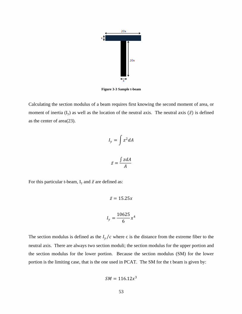
53
Figure 3-3 Sample t-beam
Calculating the section modulus of a beam requires first knowing the second moment of area, or
moment of inertia (Iy) as well as the location of the neutral axis. The neutral axis (𝑧 ) is defined
as the center of area(23).
𝐼𝑦 = 𝑧2𝑑𝐴
𝑧 = 𝑧𝑑𝐴
𝐴
For this particular t-beam, Iy and 𝑧 are defined as:
𝑧 = 15.25𝑥
𝐼𝑦 =10625
6𝑥4
The section modulus is defined as the 𝐼𝑦 𝑐 where c is the distance from the extreme fiber to the
neutral axis. There are always two section moduli; the section modulus for the upper portion and
the section modulus for the lower portion. Because the section modulus (SM) for the lower
portion is the limiting case, that is the one used in PCAT. The SM for the t beam is given by:
𝑆𝑀 = 116.12𝑥3
54
But ABS gives formulas for the section modulus. What is needed is the critical dimension, x.
𝑥 = 𝑆𝑀
116.12
3
Now given a required section modulus from ABS, the size and bending rigidity of each piece is
known.
ABS requires minimum section moduli and thicknesses for each piece and each section of hull
and deck plating, but there is also a minimum section modulus for the entire section. With the
scantlings of each piece known the total moment of inertia of the midsection can be calculated to
verify that the variant has enough strength to withstand bending. This is done in 4 steps.
1. The sum of the area of all the pieces is calculated.
2. The sum of the moment of area of all the pieces is calculated.
3. The moment of inertia of each piece about the ships base line is calculated.
4. The total moment of inertia is shifted to the neutral axis.
To complete step 3, each object's moment of inertia has to be calculated about their own
horizontal neutral axis. However many of the objects are rotated because they are placed on a
round hull. Therefore the moment of inertia must be transformed.
𝐼𝑦_𝑛𝑒𝑤 =𝐼𝑦 + 𝐼𝑧
2−𝐼𝑦 − 𝐼𝑧
2cos(2𝜃)
Where θ is the angle of rotation and Iz for the t-beam is the moment of inertia of the t-beam about
the vertical plane.
𝐼𝑧 = 𝑦2𝑑𝐴 =2005
3x4
55
To complete steps 3 and 4 the parallel axis therom must be used. The parallel axis theorem
states that the moment of inertia for an object about an arbitrary axis is the moment of inertia of
the same object about its own neutral axis added to the square of the distance between the neutral
axis and the new axis times the area.
𝐼𝑏𝑎𝑠𝑒𝑙𝑖𝑛𝑒 = 𝐼𝑦 + 𝑑2𝐴
In step 3 the moment of inertia is shifted away from a piece's neural axis to the base line, so the
d2A term is added. In step 4 however, the moment of inertia is shifted toward the section's
neutral axis, so the d2A term is subtracted.
The final section modulus of the midsection is compared to the minimum section modulus. If
the calculated section modulus is insufficient, all the scantlings are increased in 1% increments
until the section modulus of the section is met. In all test runs performed by the author, it was
never necessary to increase the scantlings of the individual pieces to meet the section’s section
modulus requirement. Stated another way, in all the trial runs preformed, if the minimum
scantlings were met for the individual pieces, the minimum section modulus was met for the
entire section.
The final calculation done in PCAT_structures is the weight of the material used to make the
hull. This will feed directly into the weight module. The weight of the material is calculated by
finding the weight of the material at each section, and then numerically integrating the section
weights along the length of the ship to get the total weight. This is added to the weight of the
transverse framing to get the total structure weight. Note that this does not include some of the
structural weight such as the transverse bulkheads and the machinery foundations.
To validate the structures calculations, a midsection was built in POSSE's section modulus editor
to match the one generated in PCAT_structures. Table 3-6 shows the comparison between the
POSSE parameters and the PCAT parameters.
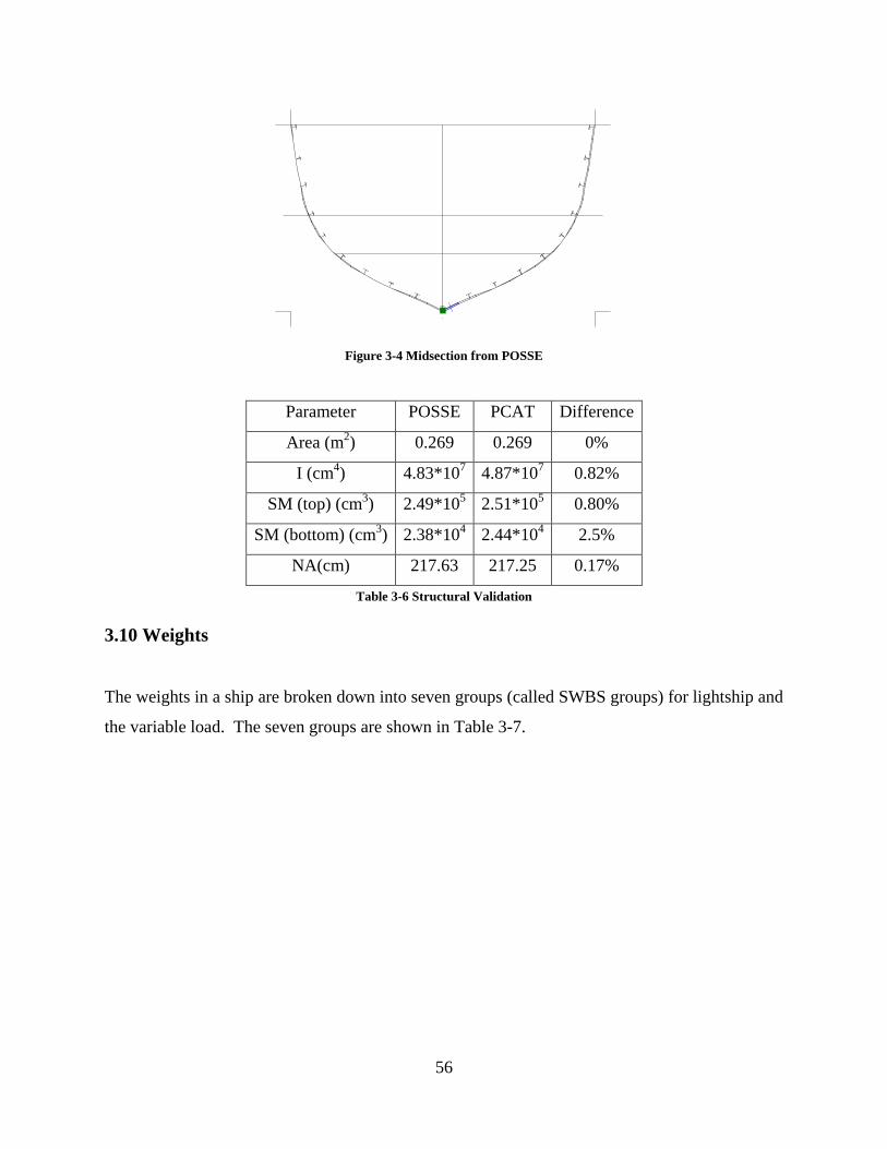
56
Figure 3-4 Midsection from POSSE
Parameter POSSE PCAT Difference
Area (m2) 0.269 0.269 0%
I (cm4) 4.83*10
7 4.87*10
7 0.82%
SM (top) (cm3) 2.49*10
5 2.51*10
5 0.80%
SM (bottom) (cm3) 2.38*10
4 2.44*10
4 2.5%
NA(cm) 217.63 217.25 0.17%
Table 3-6 Structural Validation
3.10 Weights
The weights in a ship are broken down into seven groups (called SWBS groups) for lightship and
the variable load. The seven groups are shown in Table 3-7.
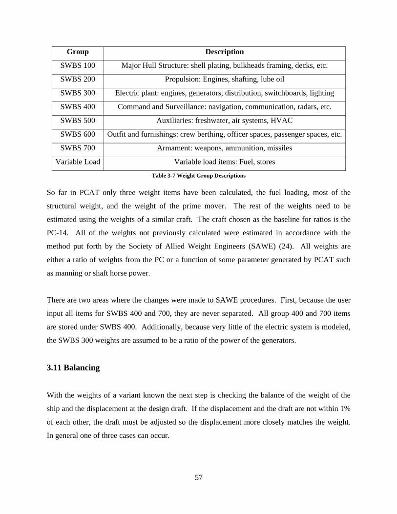
57
Group Description
SWBS 100 Major Hull Structure: shell plating, bulkheads framing, decks, etc.
SWBS 200 Propulsion: Engines, shafting, lube oil
SWBS 300 Electric plant: engines, generators, distribution, switchboards, lighting
SWBS 400 Command and Surveillance: navigation, communication, radars, etc.
SWBS 500 Auxiliaries: freshwater, air systems, HVAC
SWBS 600 Outfit and furnishings: crew berthing, officer spaces, passenger spaces, etc.
SWBS 700 Armament: weapons, ammunition, missiles
Variable Load Variable load items: Fuel, stores
Table 3-7 Weight Group Descriptions
So far in PCAT only three weight items have been calculated, the fuel loading, most of the
structural weight, and the weight of the prime mover. The rest of the weights need to be
estimated using the weights of a similar craft. The craft chosen as the baseline for ratios is the
PC-14. All of the weights not previously calculated were estimated in accordance with the
method put forth by the Society of Allied Weight Engineers (SAWE) (24). All weights are
either a ratio of weights from the PC or a function of some parameter generated by PCAT such
as manning or shaft horse power.
There are two areas where the changes were made to SAWE procedures. First, because the user
input all items for SWBS 400 and 700, they are never separated. All group 400 and 700 items
are stored under SWBS 400. Additionally, because very little of the electric system is modeled,
the SWBS 300 weights are assumed to be a ratio of the power of the generators.
3.11 Balancing
With the weights of a variant known the next step is checking the balance of the weight of the
ship and the displacement at the design draft. If the displacement and the draft are not within 1%
of each other, the draft must be adjusted so the displacement more closely matches the weight.
In general one of three cases can occur.

58
1. The variant's weight and displacement agree within 1%. If this occurs, the variant is
complete and the final cost, seakeeping, and performance analysis can occur.
2. The variant's weight and displacement are not within 1%, but there is still adequate free
board. If this occurs, two adjustments must be made to the variant. First the draft is set
to a new level as shown below.
𝑑𝑟𝑎𝑓𝑡𝑛𝑒𝑤 = 𝑑𝑟𝑎𝑓𝑡𝑜𝑙𝑑 ∗ 1 + 0.4𝑤𝑒𝑖𝑔𝑡 − ∆
∆
This is an empirical formula that was arrived at through trial and error. It adjusts the
draft as a function of the percent difference between the weight and the displacement.
Because the engine sizes are not continuous, it is very important to increase the draft
slowly so as ensure the smallest engine possible is used to power the variant. Increasing
the draft too quickly could cause an unnecessary increase in resistance and hence an
unnecessary step increase in weight due to skipping to the next larger engine. The
minimum freeboard at midships is set to 6% of ships length (25).
While the vertical and transverse offsets do not need to be adjusted, the longitudinal
offsets need to be moved so that the zero point is at the forward perpendicular. Figure
3-5 shows the profile for a nominal hull. Figure 3-6 is the offsets for the same after being
adjusted for having a weight that is more than the displacement. It is important to notice
that while the size of the hull does not change, the LBP does. So the final LBP will many
times not be the original value entered by the user, but the Overall length of the ship will
not change.
Figure 3-5 Original Profile

59
Figure 3-6 Adjusted Profile
3. The final possibility is there is no longer adequate free board. If this occurs, the variant
generates an error code and no further calculations will be performed on that variant.
The calculations for balancing are performed in PCAT_adjustoffsets and PCAT_execute.
3.12 Seakeeping
Calculating the response of ship in seas is no small task. Traditionally, seakeeping is analyzed at
the end of the design cycle after most design decisions have been made. In general if the ship
meets its minimum seakeeping requirements, little thought is put into improving seakeeping.
The most widely used method for calculating seakeeping in initial ship design is strip theory.
Ships motions of heave pitch, and roll are oscillatory in nature, due to a restoring force created
by changes in buoyancy. In strip theory, ship’s motions are modeled as a forced damped mass-
spring system (15). For instance, uncoupled heave can be modeled as
𝑀 + 𝐴33 𝜂 3 + 𝐵33𝜂 3 + 𝐶33𝜂3 = 𝐹3𝑒𝑖𝜔𝑒𝑡
Where:
M is the mass of the vessel
A33 is the added mass coefficient for heave due to heave
B33 is the damping coefficient for heave due to heave
C33 is the hydrostatic restoring coefficient for heave due to heave
F3 is the heave exciting force
𝜂3 is the instantaneous heave displacement
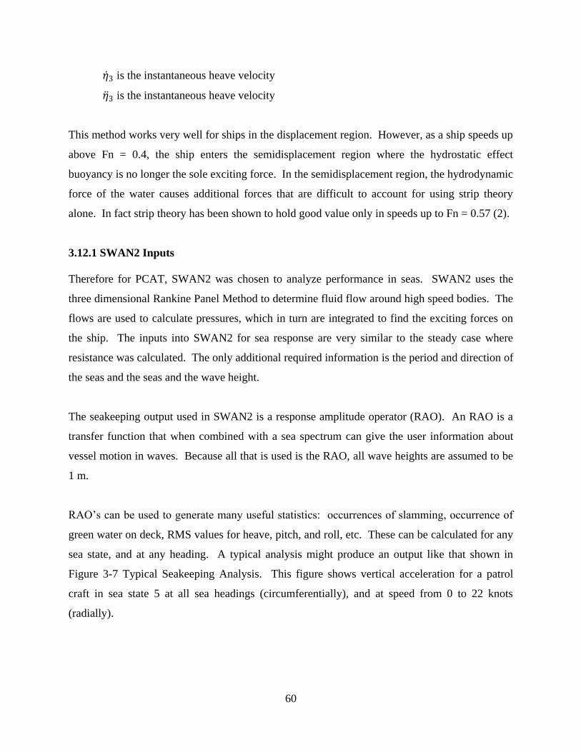
60
𝜂 3 is the instantaneous heave velocity
𝜂 3 is the instantaneous heave velocity
This method works very well for ships in the displacement region. However, as a ship speeds up
above Fn = 0.4, the ship enters the semidisplacement region where the hydrostatic effect
buoyancy is no longer the sole exciting force. In the semidisplacement region, the hydrodynamic
force of the water causes additional forces that are difficult to account for using strip theory
alone. In fact strip theory has been shown to hold good value only in speeds up to Fn = 0.57 (2).
3.12.1 SWAN2 Inputs
Therefore for PCAT, SWAN2 was chosen to analyze performance in seas. SWAN2 uses the
three dimensional Rankine Panel Method to determine fluid flow around high speed bodies. The
flows are used to calculate pressures, which in turn are integrated to find the exciting forces on
the ship. The inputs into SWAN2 for sea response are very similar to the steady case where
resistance was calculated. The only additional required information is the period and direction of
the seas and the seas and the wave height.
The seakeeping output used in SWAN2 is a response amplitude operator (RAO). An RAO is a
transfer function that when combined with a sea spectrum can give the user information about
vessel motion in waves. Because all that is used is the RAO, all wave heights are assumed to be
1 m.
RAO’s can be used to generate many useful statistics: occurrences of slamming, occurrence of
green water on deck, RMS values for heave, pitch, and roll, etc. These can be calculated for any
sea state, and at any heading. A typical analysis might produce an output like that shown in
Figure 3-7 Typical Seakeeping Analysis. This figure shows vertical acceleration for a patrol
craft in sea state 5 at all sea headings (circumferentially), and at speed from 0 to 22 knots
(radially).
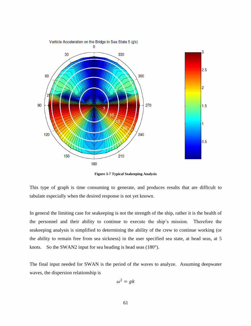
61
Figure 3-7 Typical Seakeeping Analysis
This type of graph is time consuming to generate, and produces results that are difficult to
tabulate especially when the desired response is not yet known.
In general the limiting case for seakeeping is not the strength of the ship, rather it is the health of
the personnel and their ability to continue to execute the ship’s mission. Therefore the
seakeeping analysis is simplified to determining the ability of the crew to continue working (or
the ability to remain free from sea sickness) in the user specified sea state, at head seas, at 5
knots. So the SWAN2 input for sea heading is head seas (180°).
The final input needed for SWAN is the period of the waves to analyze. Assuming deepwater
waves, the dispersion relationship is
𝜔2 = 𝑔𝑘
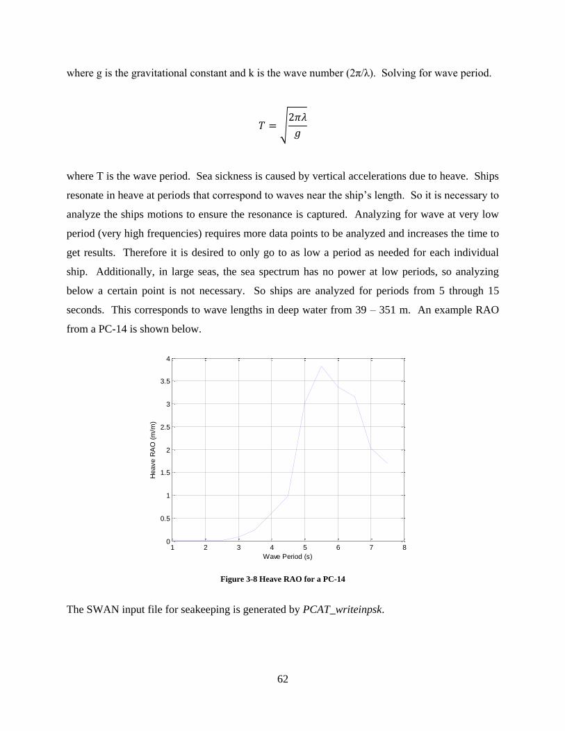
62
where g is the gravitational constant and k is the wave number (2π/λ). Solving for wave period.
𝑇 = 2𝜋𝜆
𝑔
where T is the wave period. Sea sickness is caused by vertical accelerations due to heave. Ships
resonate in heave at periods that correspond to waves near the ship’s length. So it is necessary to
analyze the ships motions to ensure the resonance is captured. Analyzing for wave at very low
period (very high frequencies) requires more data points to be analyzed and increases the time to
get results. Therefore it is desired to only go to as low a period as needed for each individual
ship. Additionally, in large seas, the sea spectrum has no power at low periods, so analyzing
below a certain point is not necessary. So ships are analyzed for periods from 5 through 15
seconds. This corresponds to wave lengths in deep water from 39 – 351 m. An example RAO
from a PC-14 is shown below.
Figure 3-8 Heave RAO for a PC-14
The SWAN input file for seakeeping is generated by PCAT_writeinpsk.
1 2 3 4 5 6 7 80
0.5
1
1.5
2
2.5
3
3.5
4
Wave Period (s)
Heave R
AO
(m
/m)

63
3.12.2 Sea Spectrum
To use the RAO generated by SWAN2, a sea spectrum is required. The Brett Schneider sea
spectrum was chosen as a standard spectrum to use because it is the ITTC standard sea spectrum
for fully developed seas. This spectrum is a two parameter spectrum
𝑆+ 𝜔 =1.25
4
𝜔𝑚4
𝜔5𝜁2𝑒−1.25 𝜔𝑚 𝜔 4
where ζ is the significant wave height (H1/3), and ωm is the modal frequency of the spectrum.
The modal frequency can be defined as
𝜔𝑚 = 0.4 𝑔
𝜁
where g is the gravitational constant.
When the user inputs a sea state into PCAT, that sea state needs to correspond to a specific sea
spectrum. To do this, the Beaufort scale (26) is used to correlate sea state to a wave height. The
wave height is then used to calculate the modal frequency.
Beaufort Number
(Sea State)
Mean Wave
height (m)
Maximum Wave
height (m)
Description
1 0.1 0.1 Calm
2 0.2 0.3 Light Breeze
3 0.6 1 Gentle Breeze
4 1 1.5 Moderate Breeze
5 2 2.5 Fresh Breeze
6 3 4 Strong Breeze
7 4 5.5 Near Gale
8 5.5 7.5 Gale
Table 3-8 Beaufort Scale
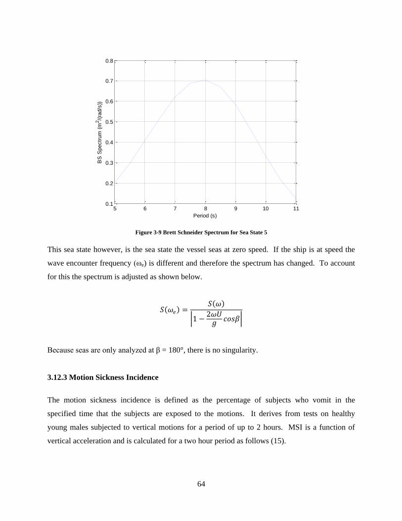
64
Figure 3-9 Brett Schneider Spectrum for Sea State 5
This sea state however, is the sea state the vessel seas at zero speed. If the ship is at speed the
wave encounter frequency (ωe) is different and therefore the spectrum has changed. To account
for this the spectrum is adjusted as shown below.
𝑆 𝜔𝑒 =𝑆 𝜔
1 −2𝜔𝑈𝑔
𝑐𝑜𝑠𝛽
Because seas are only analyzed at β = 180°, there is no singularity.
3.12.3 Motion Sickness Incidence
The motion sickness incidence is defined as the percentage of subjects who vomit in the
specified time that the subjects are exposed to the motions. It derives from tests on healthy
young males subjected to vertical motions for a period of up to 2 hours. MSI is a function of
vertical acceleration and is calculated for a two hour period as follows (15).
5 6 7 8 9 10 110.1
0.2
0.3
0.4
0.5
0.6
0.7
0.8
BS
Spectr
um
(m
2/(
rad/s
))
Period (s)

65
𝑀𝑆𝐼% = 100 ∗ 𝛷 𝑙𝑜𝑔
𝑠 3 𝑔 − 𝜇𝑀𝑆𝐼
0.4
𝜇𝑀𝑆𝐼 = −0.819 + 2.32 log𝜔𝑒 2
𝑠 = 0.798 𝑚4
where Φ(x) is the cumulative normal distribution function up to (x) for a normal distribution with
zero mean and a standard deviation of 1, 𝑠 is the ventricle acceleration of the vessel, and m4 is
the 4th
moment of the heave the heave response spectrum. The 4th
moment of the heave response
spectrum is calculated as follows
𝑚4 = 𝜔𝑒4𝑆3 𝜔𝑒 𝑑𝜔𝑒 = 𝑎3𝑅𝑀𝑆
2∞
−∞
where S3 is the heave response spectrum calculated below.
𝑆3 𝜔𝑒 = 𝑅𝐴𝑂 𝜔𝑒 2𝑆 𝜔𝑒
The MSI response and all seakeeping information is calculated in PCAT_seakeeping.
3.13 Cost
PCAT calculates two different costs, the acquisition cost and the lifecycle cost. The acquisition
cost simply uses cost estimating ratios (CER) to calculate the cost based on each weight group.
It is important to have CERs that are relevant to the ship you are building. CERs for a high tech
trimaran built of composites will be significantly different that the CERs for a patrol craft
designed in PCAT.
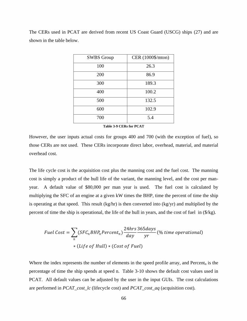
66
The CERs used in PCAT are derived from recent US Coast Guard (USCG) ships (27) and are
shown in the table below.
SWBS Group CER (1000$/mton)
100 26.3
200 86.9
300 189.3
400 100.2
500 132.5
600 102.9
700 5.4
Table 3-9 CERs for PCAT
However, the user inputs actual costs for groups 400 and 700 (with the exception of fuel), so
those CERs are not used. These CERs incorporate direct labor, overhead, material, and material
overhead cost.
The life cycle cost is the acquisition cost plus the manning cost and the fuel cost. The manning
cost is simply a product of the hull life of the variant, the manning level, and the cost per man-
year. A default value of $80,000 per man year is used. The fuel cost is calculated by
multiplying the SFC of an engine at a given kW times the BHP, time the percent of time the ship
is operating at that speed. This result (kg/hr) is then converted into (kg/yr) and multiplied by the
percent of time the ship is operational, the life of the hull in years, and the cost of fuel in ($/kg).
𝐹𝑢𝑒𝑙 𝐶𝑜𝑠𝑡 = (𝑆𝐹𝐶𝑛𝐵𝐻𝑃𝑛𝑃𝑒𝑟𝑐𝑒𝑛𝑡𝑛)24𝑟𝑠
𝑑𝑎𝑦𝑛
365𝑑𝑎𝑦𝑠
𝑦𝑟 % 𝑡𝑖𝑚𝑒 𝑜𝑝𝑒𝑟𝑎𝑡𝑖𝑜𝑛𝑎𝑙
∗ 𝐿𝑖𝑓𝑒 𝑜𝑓 𝐻𝑢𝑙𝑙 ∗ (𝐶𝑜𝑠𝑡 𝑜𝑓 𝐹𝑢𝑒𝑙)
Where the index represents the number of elements in the speed profile array, and Percentn is the
percentage of time the ship spends at speed n. Table 3-10 shows the default cost values used in
PCAT. All default values can be adjusted by the user in the input GUIs. The cost calculations
are performed in PCAT_cost_lc (lifecycle cost) and PCAT_cost_aq (acquisition cost).

67
Item Default Cost
Fuel ($/kg) 3.82
Manning ($/man-year) 80000
Table 3-10 Default Costs
3.14 Performance
The performance of each variant is calculated using the overall measure of effectiveness
(OMOE) input by the user. The OMOE is broken down into three primary MOEs: operations,
mobility, and weapons. Each of the primary levels is assigned a weight of importance, with the
sum of the primary weights equaling unity.
Mobility and operations MOEs are then broken down into secondary measures. Mobility is a
function of maximum speed, endurance, range, and draft. Each of these secondary MOEs is also
assigned a weight by the user and the sum of the mobility weights is also unity. Operations is a
function of main deck area, in-hull area, manning and seakeeping. The operations weights are
assigned in the same manner as the mobility weights. The weapons MOE is assigned by the user
and is not broken down to a second level.
Each secondary MOE is given a value based on the user inputs and PCAT calculations. The user
either specifies the threshold and goal values, or the threshold is set at the worst value of a
particular parameter and goal is set at the best. The threshold value for a given parameter is
given a MOE of zero. The goal is given a value of one. All values in between are linearly
interpolated between 0 and 1 as shown in Figure 3-10.

68
Figure 3-10 Example MOE
The total operation MOE is then:
𝑀𝑂𝐸𝑂𝑃𝑆 = 𝑊𝐼𝐻𝐴𝑅𝐸𝐴𝑀𝑂𝐸𝐼𝐻𝐴𝑅𝐸𝐴 + 𝑊𝑀𝐷𝐴𝑅𝐸𝐴𝑀𝑂𝐸𝑀𝐷𝐴𝑅𝐸𝐴 + 𝑊𝑀𝐴𝑁𝑀𝑂𝐸𝑀𝐴𝑁 + 𝑊𝑆𝐸𝐴𝑀𝑂𝐸𝑆𝐸𝐴
Where W represents the user assigned weighting value. The mobility MOE is calculated in the
same way. The overall MOE is then
𝑂𝑀𝑂𝐸 = 𝑊𝑂𝑃𝑆𝑀𝑂𝐸𝑂𝑃𝑆 + 𝑊𝑀𝑂𝐵𝐼𝐿𝐼𝑇𝑌𝑀𝑂𝐸𝑀𝑂𝐵𝐼𝐿𝐼𝑇𝑌 + 𝑊𝑊𝐸𝑃𝑆𝑀𝑂𝐸𝑊𝐸𝑃𝑆
3.15 Rejection Criteria
Ships can be rejected for many different reasons. In each case the rejection will generate an error
code so the user will know why the rejection occurred. The list below is all of the reasons a ship
may be rejected
Froude number mismatch – One of the major limitations of PCAT is the range over
which resistance can be calculated. If the Froude number of the maximum speed, the

69
endurance speed (if not set to default) or any of the speeds in the speed profile are less
than 0.1 or greater than 0.6, the program will not converge on a final design for that
variant, and an error code will be generated.
Inadequate area – If the main deck area is less than the area required for the weapons, or
the internal area is less than the area required for the weapons and the prime movers, the
program will not converge on a final design for that variant, and an error code will be
generated.
Inadequate GM – If the GM for a particular variant less than 0.5 m, the program will not
converge on a final design for that variant, and an error code will be generated.
Unable to converge – If there is a significant mismatch between the weight and the
displacement of the ship and the freeboard at midships is reduced to less than 4% of the
overall length, the program will not converge on a final design for that variant, and an
error code will be generated.

70
4.0 Optimization for PCAT
Each individual ship run or experiment on PCAT takes nominally 1 hour to accomplish. While
that may not seem like an incredibly long time, to do a full factorial search on 13 variables at
only 4 levels each, would require 134 or 28,561 hours or about 3 years. 3 years is clearly not an
acceptable time frame for results on an early stage design program, so some optimization must
be done to minimize the number of experiments and still allow for useful results that can lead a
designer to either perform additional experiments or to make design decisions.
4.1 Response Surface Methodology
Response surface methodology (RSM) is a collection of statistical and mathematical techniques
useful for developing, improving, and optimizing a process. Additionally, it can be used to
design, develop, and formulate new products, or improve existing designs. RSM was originally
created by G. E. Box and K. B. Wilson in 1951. It uses a sequence of specific experiments
designed to capture a snap shot of the entire design space and then uses regression techniques to
derive the relationship between several independent input variables (xi) and one or more
response variables (y) (28).
Because of the regression techniques used, RSM can only be used with continuous variables.
For the case of PCAT, that limits the variables to:
L
L/B
L/D
Deck height
Frame spacing,
LCG/L
KG/D
Manning
Range
71
Number of Shafts
These will be the 10 independent variables for RSM. The remaining design variables that can
assume different levels are:
Parent hull
Hull Material
Weapon group
Choice of Waterjets or Propellers
These variables will be considered discrete and will be addressed later in the chapter. The
discrete variables will all be fixed at one level (the first level entered is chosen if the user input
multiple levels) for the entire RSM analysis. There are many other design variables in PCAT
such as the speed profile and the percentage of the manning that is officer, enlisted, or senior
enlisted, however these design variables are held fixed for all ships in the run. Therefore it is not
necessary to include these variables in the RSM.
PCAT produces three different responses.
Acquisition cost
Lifecycle Cost
Performance (OMOE)
These variables are the response variables for RSM in PCAT.
In general the user wants to know what the effect changing an input (xi) has on the response (y).
A single response can be characterized by
𝑦 = 𝑓(𝑥1 , 𝑥2 , 𝑥3 ,… , 𝑥𝑛)
If the system was assumed to be linear and first order, then the response could be characterized
by
𝑦 = 𝛽0 + 𝛽1𝑥1 + 𝛽2𝑥2 + ⋯+ 𝛽𝑛𝑥𝑛
72
This first order model is called a main effects model because it only includes the effects of the
variables themselves. If there is an interaction between these variables, it is not captured by a
main effects model. Often the first order model is inadequate to capture the response. Therefore
a higher order model is used in PCAT.
If first order effects are considered as well as interaction and quadratic effects, the model would
be represented by
𝑦(𝑥) = 𝛽0 + 𝛽1𝑥1 + 𝛽2𝑥2 + 𝛽11𝑥12 + 𝛽22𝑥2
2 + 𝛽12𝑥1𝑥2 …
Or more generally, for n variables
𝑦(𝑥) = 𝛽0 + 𝛽𝑖𝑥𝑖
𝑛
𝑖=0
+ 𝛽𝑖𝑗 𝑥𝑖𝑥𝑗
𝑛
𝑖<𝑗
+ 𝛽𝑖𝑖𝑥𝑖2
𝑛
𝑖=0
This model is called a second order, or quadratic model. This is the model that will be used in
PCAT.
4.2 Designing the Experiments
As previously discussed, it is important to choose the experiments in such a way that the entire
design space is covered in a minimum number of experiments. Central Composite Designs
(CCDs) are appropriate for calibrating quadratic models(28) (29). There are three types of
CCDs: circumscribed, inscribed, and faced. Examples are shown below.

73
Figure 4-1 Circumscribed CCD
Figure 4-2 Inscribed CCD

74
Figure 4-3 Faced CCD
Each CCD consists of a factorial design (the corners of a cube) together with center and star
points that allow for estimation of second-order effects. For a full quadratic model with n factors,
CCDs have enough design points to estimate the coefficients in a full quadratic model with n
factors (29).
The type of CCD is determined by the number or levels a variable can take and by the desired
properties of the design. The following table below summarizes properties of the three CCD
designs (29).
Design Factor
Levels
Uses Outside
Points Accuracy
Circumscribed 5 Yes Good over the entire design space
Inscribed 5 No Good over the central subset of the design space
Faced 3 No Fair over the entire design space, though poor
for pure quadratic coefficients
Table 4-1 Properties of CCDs
For the bounds of the experiments, the limits of the user inputs are selected. Therefore, it is not
desired to use any points outside the user inputted range. This eliminates the circumscribed
CCD. Additionally is not desired to diminish the effects of the quadratic coefficients, therefore
the Inscribed CCD was chosen to design all experiments. It is important to note the inscribed
75
CCD is not as accurate around the edges of the design space as the other methods. For this
reason, when using RSM in PCAT, the user should be aware that the results near the edges of the
design space may not be as accurate and should be fully modeled.
For 10 variables the inscribed CCD requires a minimum of 149 experiments. This is much more
reasonable, and should take on the order of 6 days. If the user can fix only two factors, such as
frame spacing and LCG/L, then the number of experiments is down to 81 which should take on
the order of 3.5 days. The variable levels are assigned only for variables that have a different
maximum and minimum, thereby ensuring that no experiments are unnecessarily repeated. The
experiments are designed in PCAT_rsm. Once the experiments are designed, the ship building
and analysis is performed in the same method as shown in chapter 3.
4.3 Analysis and Optimization
After the analysis is complete with all three response variables calculated for each ship, linear
regression is used to determine the coefficients for the quadratic model. In general at this point
in RSM, the user would use graphical tools to look at the effects of specific variable input on a
response using the model created, allowing the user to find an optimal or near optimal solution
with little additional calculation from the program. However, for this design there are two issues
that make this difficult.
First, there are multiple responses that will not optimize at the same point. Performance and cost
are inherently opposed. The highest performing ship will likely be the most expensive. This
makes it difficult to define THE optimal ship, much less find it. The simplest way to alleviate
this concern is to allow users to look at this trade off, use good engineering judgment, and
choose ships they would like to optimize around. To do this, a chart that shows ships cost and
performance of ships over a wide range of variable inputs is given to the user. The ships will
form a pareto frontier and the user then is allowed to choose what ships to use a basis for further
study.

76
The range of ships used to create the pareto frontier takes every variable analyzed for in the RSM
and does a full factorial search at 5 levels using the quadratic model to determine the responses
instead of the original program. This is done in PCAT_rsmfinal. A sample chart is shown
below.
Figure 4-4 Sample Cost/Performance chart
The user can then drill down to find information about high performing, low cost ships. In
general the ships analyzed will be in the top right portion of this chart. With a narrower range of
variables, the user now needs to run a second set of analysis at a full factorial level that will
allow for the optimization of discrete variables. This is just like running PCAT originally with a
full factorial set of experiments. However, the design space has been narrowed to now limit the
number of experiments. Chapter 5 gives an example of this process.
77
5.0 Using PCAT
This chapter describes the process for one particular example of PCAT using RSM on the first
run, and a full factorial analysis on the second.
5.1 Inputs
User inputs for the first run are shown below. These variables were chosen so RSM could be
used.
Geometry
Length was given a range of 27.4 m to 33.5 m.
L/B was given a range of 4.5 to 5.206.
L/D was given a range of 7.0 to 8.148.
The PC-14 was chosen for the parent hull.
Deck height was set to be 2.75 m.
Loading
KG/D was set a 0.6.
The LCG was set to default.
The material was set to ordinary strength steel.
The frame spacing was set to 1.5 m.
Machinery
Only 1 engine per shaft was allowed.
Each ship had 2 shafts.
Only propellers were allowed.
Speed

78
The maximum speed was set to 20 kts.
The endurance speed was set to default.
The range was set from 700 to 800 nm.
The speed profile is [5 kts-20% 10 kts-35% 12.5 kts-25% 15 kts-15% 20kts-5%]
Weapons – The weapons profiles was set as shown in Table 5-1.
ID Weight (mton) DH area (m2) IH area (m
2) Power (kW) KG/D WMOE Cost (k$)
Med 8 14 27.9 120 1 0.6 2000
Table 5-1 Input Parameters for Weapons
Manning – 15 men on board with 13.3% officer, 13.3% CPO, and 73.3% enlisted.
Seakeeping – The Sea State was set to Sea State 5.
Cost – All the cost values were left at their default values.
OMOE – All the secondary MOEs goal and threshold values were left to default. The weights
for all the MOEs are:
Maximum speed - 0.25
Endurance - 0.25
range - 0.25
Draft - 0.25
Main deck area - 0.30
In-hull area - 0.30
Manning - 0.20
Seakeeping - 0.20
Operations - 0.40
Mobility - 0.40
Weapons - 0.20
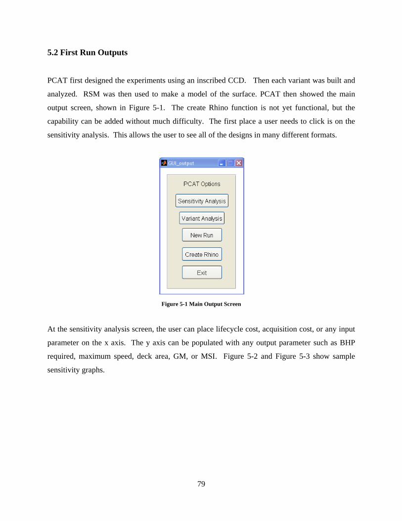
79
5.2 First Run Outputs
PCAT first designed the experiments using an inscribed CCD. Then each variant was built and
analyzed. RSM was then used to make a model of the surface. PCAT then showed the main
output screen, shown in Figure 5-1. The create Rhino function is not yet functional, but the
capability can be added without much difficulty. The first place a user needs to click is on the
sensitivity analysis. This allows the user to see all of the designs in many different formats.
Figure 5-1 Main Output Screen
At the sensitivity analysis screen, the user can place lifecycle cost, acquisition cost, or any input
parameter on the x axis. The y axis can be populated with any output parameter such as BHP
required, maximum speed, deck area, GM, or MSI. Figure 5-2 and Figure 5-3 show sample
sensitivity graphs.
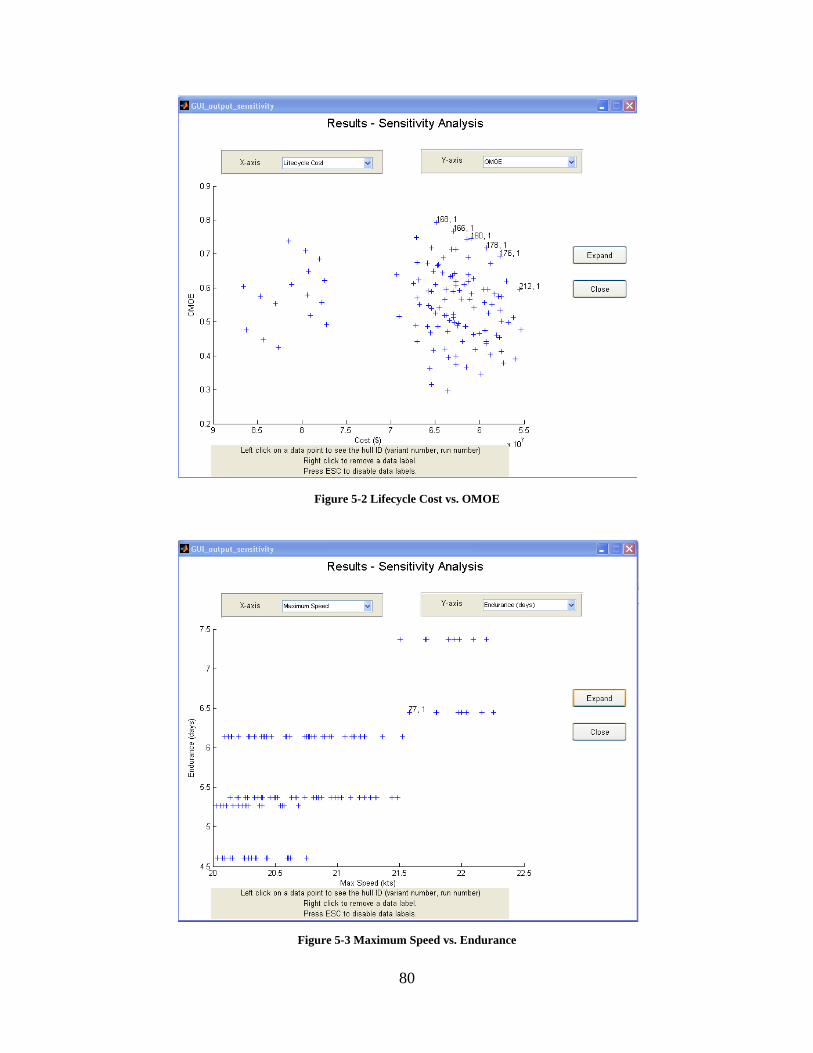
80
Figure 5-2 Lifecycle Cost vs. OMOE
Figure 5-3 Maximum Speed vs. Endurance
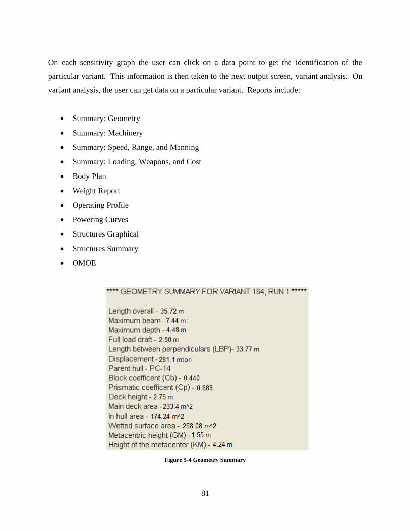
81
On each sensitivity graph the user can click on a data point to get the identification of the
particular variant. This information is then taken to the next output screen, variant analysis. On
variant analysis, the user can get data on a particular variant. Reports include:
Summary: Geometry
Summary: Machinery
Summary: Speed, Range, and Manning
Summary: Loading, Weapons, and Cost
Body Plan
Weight Report
Operating Profile
Powering Curves
Structures Graphical
Structures Summary
OMOE
Figure 5-4 Geometry Summary

82
Figure 5-5 Speed, Range, and Manning Summary
Figure 5-6 Machinery Summary

83
Figure 5-7 Loading Weapons, and Cost Summary
Figure 5-8 Body Plan

84
Figure 5-9 Weight Report
Figure 5-10 Speed Profile

85
Figure 5-11 Structures Graphical
Figure 5-12 Structures Summary
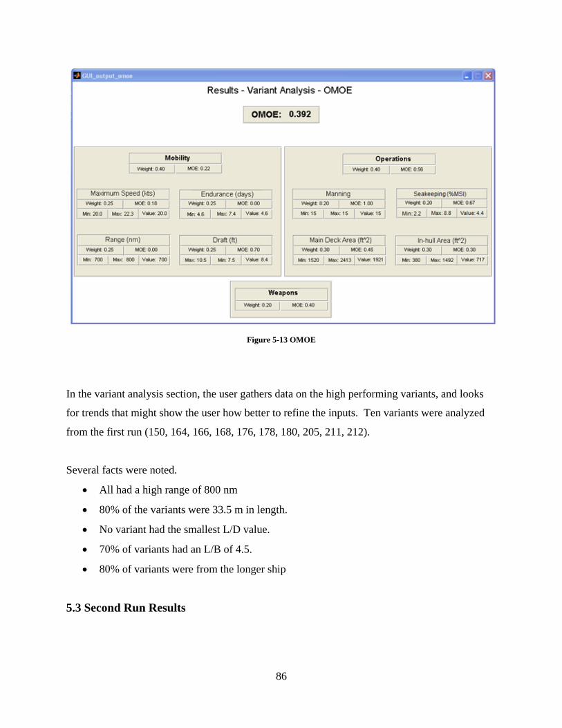
86
Figure 5-13 OMOE
In the variant analysis section, the user gathers data on the high performing variants, and looks
for trends that might show the user how better to refine the inputs. Ten variants were analyzed
from the first run (150, 164, 166, 168, 176, 178, 180, 205, 211, 212).
Several facts were noted.
All had a high range of 800 nm
80% of the variants were 33.5 m in length.
No variant had the smallest L/D value.
70% of variants had an L/B of 4.5.
80% of variants were from the longer ship
5.3 Second Run Results
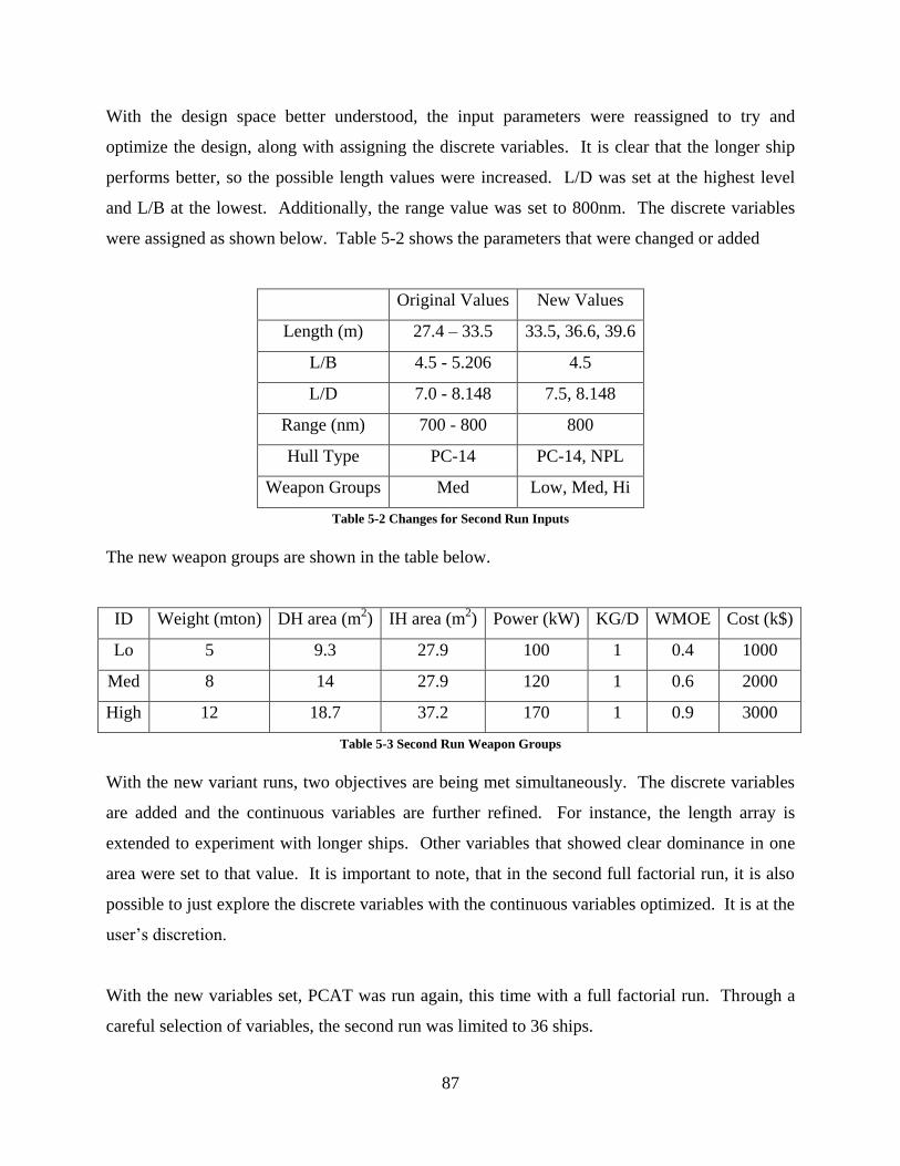
87
With the design space better understood, the input parameters were reassigned to try and
optimize the design, along with assigning the discrete variables. It is clear that the longer ship
performs better, so the possible length values were increased. L/D was set at the highest level
and L/B at the lowest. Additionally, the range value was set to 800nm. The discrete variables
were assigned as shown below. Table 5-2 shows the parameters that were changed or added
Original Values New Values
Length (m) 27.4 – 33.5 33.5, 36.6, 39.6
L/B 4.5 - 5.206 4.5
L/D 7.0 - 8.148 7.5, 8.148
Range (nm) 700 - 800 800
Hull Type PC-14 PC-14, NPL
Weapon Groups Med Low, Med, Hi
Table 5-2 Changes for Second Run Inputs
The new weapon groups are shown in the table below.
ID Weight (mton) DH area (m2) IH area (m
2) Power (kW) KG/D WMOE Cost (k$)
Lo 5 9.3 27.9 100 1 0.4 1000
Med 8 14 27.9 120 1 0.6 2000
High 12 18.7 37.2 170 1 0.9 3000
Table 5-3 Second Run Weapon Groups
With the new variant runs, two objectives are being met simultaneously. The discrete variables
are added and the continuous variables are further refined. For instance, the length array is
extended to experiment with longer ships. Other variables that showed clear dominance in one
area were set to that value. It is important to note, that in the second full factorial run, it is also
possible to just explore the discrete variables with the continuous variables optimized. It is at the
user’s discretion.
With the new variables set, PCAT was run again, this time with a full factorial run. Through a
careful selection of variables, the second run was limited to 36 ships.
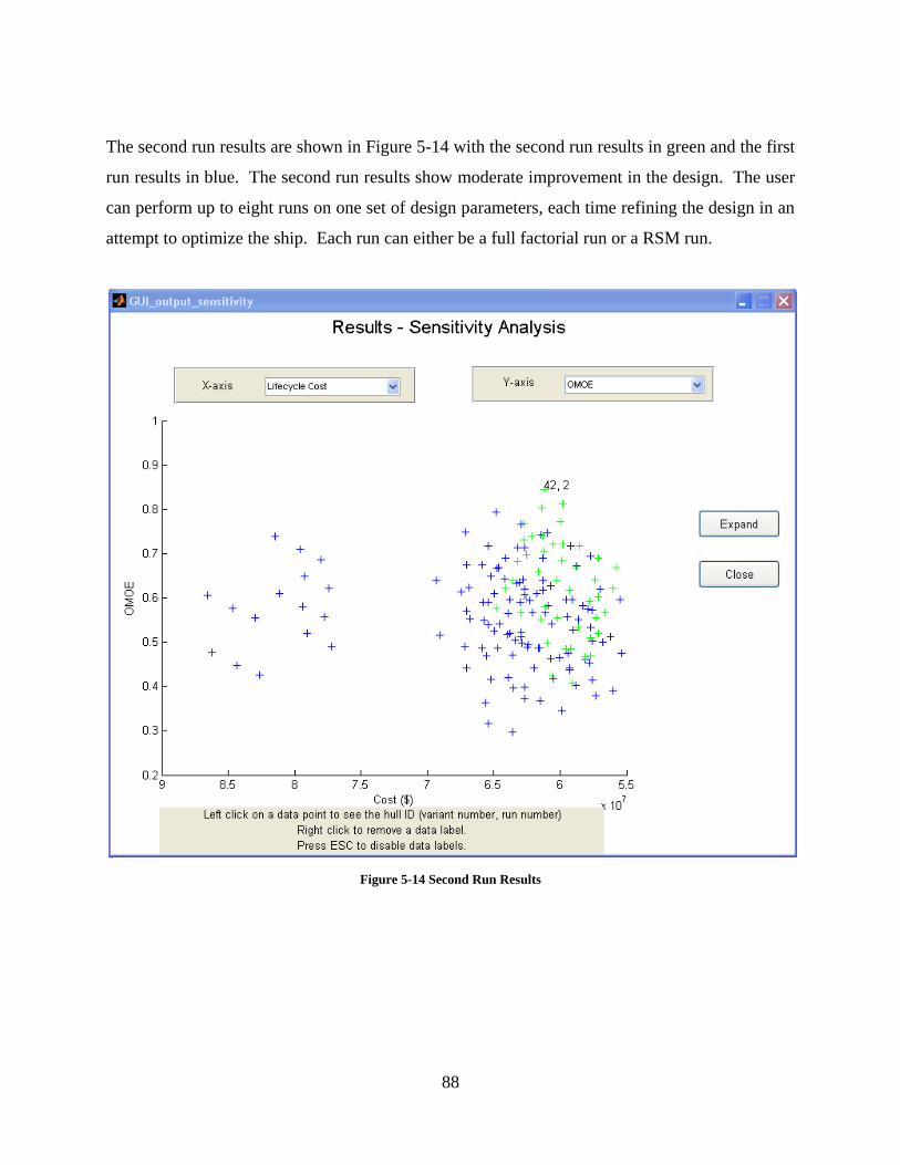
88
The second run results are shown in Figure 5-14 with the second run results in green and the first
run results in blue. The second run results show moderate improvement in the design. The user
can perform up to eight runs on one set of design parameters, each time refining the design in an
attempt to optimize the ship. Each run can either be a full factorial run or a RSM run.
Figure 5-14 Second Run Results

89
6.0 Whole Ship Validation
To validate the entire model, PCAT was used to create a Cyclone class patrol craft. The PC-14
is a member of this class of ships and that specific ship was used for validation.
The first step in validation is defining the PCAT inputs for the PC-14. Most inputs were taken
from the U.S. Navy’s ASSET model of the PC-14 (10). Items marked with an asterisk (*) were
assumed values. OMOE values are irrelevant for this experiment and therefore are not listed.

90
Variable Value
Length 50.7 m
L/B 6.95
L/D 10.35
Parent Hull PC-14
Deck Height* 2.6 m
LCG/L Default
KG/D 0.6
Frame Spacing* 1.5 m
Material6 AH36
Engines per shaft 1
Shafts 4
Waterjets No
Manning 28 men
Manning Breakdown
14.3% Officer
14.3% CPO
71.4% Enlisted
Maximum Speed 25.1 kts
Endurance Speed 12 kts
Range 2649nm
Speed Profile*
5 kts - 20%
10 kts - 40%
15 kts - 25%
20 kts - 10%
25 kts - 5%
Seastate 5
Cost Default Values
Table 6-1 PCAT Values for Validation
6 There was no exact match for the material used in the PC-14. AH-36 was chosen because of the similarity in σy
and σUTS. For PC-14 HSS, σy = 352 N/mm2, σUTS = 496 N/mm2. For AH-36, σy = 355 N/mm2, σUTS = 555 N/mm2.

91
The weapons onboard the PC-14 are listed below (30). The PC-14 is fit with the following
weapons systems:
1 sextuple SAM stinger
1 Bushmaster 25mm mk-38 25mm gun
4 - 12.7 mm machine guns
4 – 7.62 mm maching guns
2 – 40 mm Mk 19 grenade launchers
2 – Mk 52 sextuple and Wallop Super Barricade Mk 3 chaff launchers
The PC-14 also has the following command and control systems (30):
Privateer APR-39 radar electronic surveillance measures (ESM) system
Marconi VISTAR IM 405 IR weapons control system
2 – Sperry RASCAR; E/F/I/J-band surface search radars
1 – Wesmar; hull mounted active high frequency hull mounted active sonar
To calculate the weight of this equipment, the ASSET PC-14 model was used. The area
requirement came from the ASSET model as well. To calculate the cost of the SWBS groups
400 and 700, the USCG CERs for SWBS groups 400 and 700 were used. This generated the
weapons input below.
6.1 Validation Results
The validation results shown below are grouped by PCAT report. For those response values with
no comparable value, the response is just list for informational purposes.
Table 6-2 PCAT Weapons Input for Whole Ship Validation
ID Weight (mton) DH area (m2) IH area (m2) Power (kW) KG/D WMOE Cost (k$)
PC-14 20.0 564 21.2 25* 1* 1* 468.7
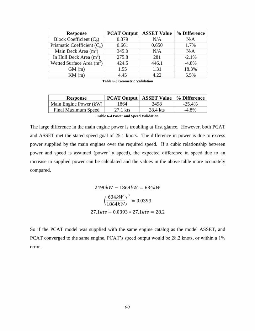
92
Response PCAT Output ASSET Value % Difference
Block Coefficient (Cb) 0.379 N/A N/A
Prismatic Coefficient (Cp) 0.661 0.650 1.7%
Main Deck Area (m2) 345.0 N/A N/A
In Hull Deck Area (m2) 275.8 281 -2.1%
Wetted Surface Area (m2) 424.5 446.1 -4.8%
GM (m) 1.55 1.31 18.3%
KM (m) 4.45 4.22 5.5% Table 6-3 Geometric Validation
Response PCAT Output ASSET Value % Difference
Main Engine Power (kW) 1864 2498 -25.4%
Final Maximum Speed 27.1 kts 28.4 kts -4.8% Table 6-4 Power and Speed Validation
The large difference in the main engine power is troubling at first glance. However, both PCAT
and ASSET met the stated speed goal of 25.1 knots. The difference in power is due to excess
power supplied by the main engines over the required speed. If a cubic relationship between
power and speed is assumed (power3 α speed), the expected difference in speed due to an
increase in supplied power can be calculated and the values in the above table more accurately
compared.
2490𝑘𝑊 − 1864𝑘𝑊 = 634𝑘𝑊
634𝑘𝑊
1864𝑘𝑊
3
= 0.0393
27.1𝑘𝑡𝑠 + 0.0393 ∗ 27.1𝑘𝑡𝑠 = 28.2
So if the PCAT model was supplied with the same engine catalog as the model ASSET, and
PCAT converged to the same engine, PCAT’s speed output would be 28.2 knots, or within a 1%
error.

93
Response PCAT Output ASSET Value % Difference
SWBS 100 (mton) 222.8 224.9 -0.95%
SWBS 200 (mton) 32.9 75.8 -56.5%
SWBS 300 (mton) 27.3 20.5 24.9%
SWBS 400 and 700 (mton) 20.1 20.1 0%
SWBS 500 (mton) 54.8 66.2 -17.2%
SWBS 600 (mton) 31.2 32.6 -4.3%
SWBS WF41 (mton) 44.2 40.8 8.3%
Total Displacement (mton) 469.7 480.8 -2.3%
Table 6-5 Weight Validation
These results are, in total, very pleasing. The largest weight errors occur in two SWBS groups,
the propulsion (SWBS 200) group and the electric (SWBS 300) group. The electric group is
very roughly modeled in PCAT and it is understandable that the weight would be more than 25%
off. It is surprising though that the propulsion group so far off. After significant investigation,
there was no known cause for this disparity.
Because the Navy did not use ABS guide lines for the designing of the structures, it would be
erroneous to compare the individual pieces in the structures module from PCAT and ASSET.
However, by comparing the section modulus and the location of the neutral axis, it can be shown
that the structures are quite similar.
Response PCAT Output ASSET Value % Difference
Neural Axis to Keel Distance (m) 2.47 2.39 3.3%
Section Modulus to Keel (m-cm2) 3467 3093 12.1%
Table 6-6 Structural Validation
The PC-14 was ordered in 1997 for $23.19 million (31). Accounting for inflation to 2008 (32)
(CERs are in 2008 dollars) gives a cost of the actual PC-14 in 2008 dollars of $31.84 million

94
Response PCAT Output Actual cost % Difference
Acquisition Cost $24.83M $31.84M -22.0%
Lifecycle Cost $107.43 N/A N/A
Table 6-7 Cost Validation
The acquisition cost results are quite good. The most important aspect of cost in PCAT is for
comparison purposes, so to be within 25% on a rough model is excellent. Calculating the actual
lifecycle cost for an actual decommissioned ship is difficult at best. For a ship during its service
life, it is near impossible, and the PC-14 is still in service. Additionally, the lifecycle cost
calculated in PCAT only includes manning and fuel considerations, and not many of the other
important lifecycle cost factors such as maintenance and repair. Even if an actual lifecycle cost
was available, it would not be worthwhile to compare the actual value to PCAT’s value.
Therefore no comparison for lifecycle cost is given.
In total, PCAT’s results seem reasonable and comparable with an actual ship.

95
7.0 Conclusion
The goal of PCAT was:
Using a systems approach, a Patrol Craft Assessment Tool (PCAT) will be created and
tested to aide designers in the initial design and assessment of patrol craft of < 90 m
operating in the semi-displacement or displacement regions. PCAT will be an open
source MATLAB code that incorporates resistance, engine selection, structures, mission
profiles, seakeeping, cost, and performance into one design program to aide a designer
in optimizing a patrol craft.
For the most part this goal was met, though there are several areas in which PCAT could be
improved.
7.1 Areas for Future Work
In a model such as the one created in PCAT, there are always areas to improve. The first area for
improvement is an interface problem between Matlab and SWAN2. As SWAN2 solves for flow
around the hull it goes through a three step process. First a spline sheet geometry file is
generated. Next the boundary integral equation is setup and a solution is determined for the base
flow is solved. Finally, the boundary integral equation is solved for the problem. Between each
of these steps SWAN requires a carriage return to be hit. SWAN2 and hence PCAT will wait for
a carriage return before moving on to the next step. This means that the user must continually hit
enter on their keyboard for PCAT to advance. While this is just a technical “glitch” it is a very
inconvenient one and should be fixed if at all possible in future work with PCAT.
Another area to help improve the speed of the program would be the creation of a function to
parse the design information before the ships are analyzed and recombine the results at a later
point in time. This would allow the user to take the information to multiple computers to
dramatically lower the analysis time.
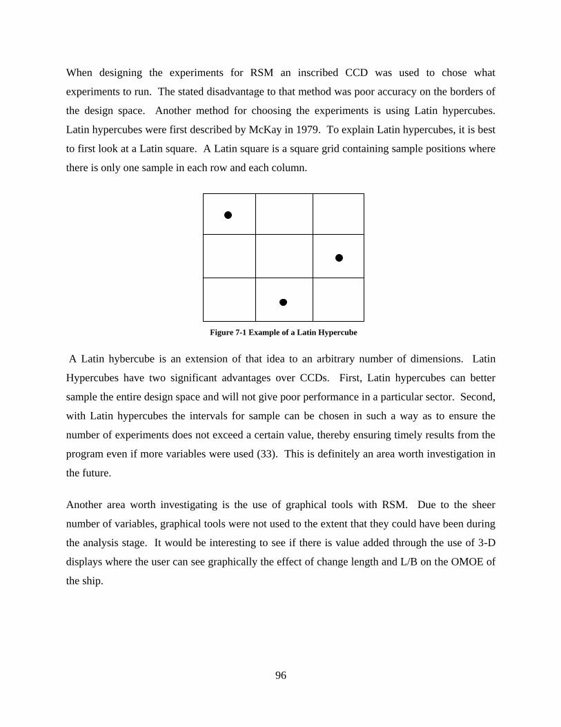
96
When designing the experiments for RSM an inscribed CCD was used to chose what
experiments to run. The stated disadvantage to that method was poor accuracy on the borders of
the design space. Another method for choosing the experiments is using Latin hypercubes.
Latin hypercubes were first described by McKay in 1979. To explain Latin hypercubes, it is best
to first look at a Latin square. A Latin square is a square grid containing sample positions where
there is only one sample in each row and each column.
A Latin hybercube is an extension of that idea to an arbitrary number of dimensions. Latin
Hypercubes have two significant advantages over CCDs. First, Latin hypercubes can better
sample the entire design space and will not give poor performance in a particular sector. Second,
with Latin hypercubes the intervals for sample can be chosen in such a way as to ensure the
number of experiments does not exceed a certain value, thereby ensuring timely results from the
program even if more variables were used (33). This is definitely an area worth investigation in
the future.
Another area worth investigating is the use of graphical tools with RSM. Due to the sheer
number of variables, graphical tools were not used to the extent that they could have been during
the analysis stage. It would be interesting to see if there is value added through the use of 3-D
displays where the user can see graphically the effect of change length and L/B on the OMOE of
the ship.
Figure 7-1 Example of a Latin Hypercube
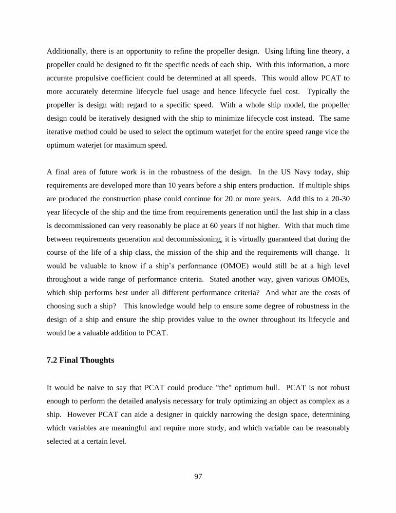
97
Additionally, there is an opportunity to refine the propeller design. Using lifting line theory, a
propeller could be designed to fit the specific needs of each ship. With this information, a more
accurate propulsive coefficient could be determined at all speeds. This would allow PCAT to
more accurately determine lifecycle fuel usage and hence lifecycle fuel cost. Typically the
propeller is design with regard to a specific speed. With a whole ship model, the propeller
design could be iteratively designed with the ship to minimize lifecycle cost instead. The same
iterative method could be used to select the optimum waterjet for the entire speed range vice the
optimum waterjet for maximum speed.
A final area of future work is in the robustness of the design. In the US Navy today, ship
requirements are developed more than 10 years before a ship enters production. If multiple ships
are produced the construction phase could continue for 20 or more years. Add this to a 20-30
year lifecycle of the ship and the time from requirements generation until the last ship in a class
is decommissioned can very reasonably be place at 60 years if not higher. With that much time
between requirements generation and decommissioning, it is virtually guaranteed that during the
course of the life of a ship class, the mission of the ship and the requirements will change. It
would be valuable to know if a ship’s performance (OMOE) would still be at a high level
throughout a wide range of performance criteria. Stated another way, given various OMOEs,
which ship performs best under all different performance criteria? And what are the costs of
choosing such a ship? This knowledge would help to ensure some degree of robustness in the
design of a ship and ensure the ship provides value to the owner throughout its lifecycle and
would be a valuable addition to PCAT.
7.2 Final Thoughts
It would be naive to say that PCAT could produce "the" optimum hull. PCAT is not robust
enough to perform the detailed analysis necessary for truly optimizing an object as complex as a
ship. However PCAT can aide a designer in quickly narrowing the design space, determining
which variables are meaningful and require more study, and which variable can be reasonably
selected at a certain level.

98
It is not intended that a designer use PCAT as currently coded. Rather a designer should
consider the requirements of their ship and ensure that PCAT adequately addresses the design
challenges. Are there additional performance factors that should be included in OMOE? Is the
model detailed enough in the areas that are important for each specific design? Questions like
these must be asked and answered to ensure that the results or meaningful. This thesis was
written and PCAT was coded in such a way as to facilitate change and improvement to the
program and to allow a designer analyze the tradeoffs involved in ship design..

99
8.0 Works Cited
1. On the numerical prediction of seakeeping and structural loads of high-speed vessels.
Zaraphonitis, George and Papanikolaou, Apostolos. Athens, Greece : Applied Ocean
Research , 2004, Vol. 26.
2. The High-Speed Displacement Ship Systematic Hull Forms - Seakeeping Characteristics.
Blok, Jan and Beukelman, Wim. New York City : The Society of Naval Architects and Marine
Engineers, 1984, Vol. 92.
3. Semi-planing Vessels in a Seaway, Comparative Prediction of Operability. Wijngaarden, A.
and Beukelman, W. Wageningen, The Netherlands : Maratime Research Institute, 1985, Vol. 2.
From "Workshop on Developments in Hull Form Design".
4. Concept Exploration - an Approach to Small Warship Design. Eames, M.C. and
Drummond, T. G. London : The Royal Institue of Naval Architects, 1976, Royal Institution of
Naval Architects Transactions, Vol. 119.
5. Ulrich, Karl T. and Eppinger, Steven D. Product Design and Development. 3. New York :
McGraw-Hill/Irwin, 2004.
6. Maier, Mark M and Rechtin, Eberhardt. The Art of Systems Architecting. New York : CRC
Press, 2002. 0-8493-0440-7.
7. American Bureau of Shipping. ABS Rules for Materials and Welding 2008, Part 2.
Houston : American Bureau of Shipping, 2007.
8. World Meteorological Organization. Manual on Codes, International Codes Volume I.1.
Geneva, Switzerland : World Meteorological Organization, 2009. ISBN 978-92-63-10306-2.
9. Bailey, D. Maratime Technology Monograph No. 4: The NPL High Speed Round Bilge
Displacement Hull Series. s.l. : The Royal Institue of Naval Architects, 1976.
10. PC-1 Cyclone class Patrol Coastal Boats. FAS Military Analysis Network. [Online] May 09,
2000. [Cited: April 18, 2008.] http://www.fas.org/man/dod-101/sys/ship/pc-1.htm.
11. Carderock Division, Naval Surface Warfare Center. PC-14 file. [Advanced Surface Ship
Evaluation Tool] Bethesda, VA : Carderock Division, Naval Surface Warfare Center, 2008.
12. Lewis, Edward V., [ed.]. Principles of Naval Architecture. Jersey City : The Society of
Naval Architects and Marine Engineers, 1988. Vol. 1.
13. Gillme, Thomas C. and Johnson, Bruce. Introduction to Naval Architecture. Annapolis :
Naval Institute Press, 1982. 0-87021-318-0.
14. Naval Surface Warfare Center, Carderock Division. Residual Resistance. [ASSET help
file] Bethesda Maryland : Naval Sea Systems Command , 2006.
15. Formation Design Systems. Hull Speed Users Manual. [PDF] s.l. : Formation Design
Systems, 2004.
16. Resistance of a Systematic Series of Semiplaning Transom-Stern Hulls. Compton, Roger H.
4, s.l. : Society of Naval Architects and Marine Engineers, 1986, Marine Technology , Vol. 23.
17. Simulation Based Resistance and Seakeeping Performance of High Speed Monohull and
Multihull Vessels Equipped with Motion Control Lifting Appendages. Sclavounos, Paul, et al.
Ischia, Italy : s.n., 2003. FAST 2003 Conference.
18. Watson, D.G.M. Practical Ship Design. New York : Elsevier, 1998. 0 08 0429998.
19. Woud, Hans and Stapersma, Douwe. Design of Propulsion and Electric Power Generation
Systems. London : The Institue of Marine Enginerring, Science and Technology, 2003. 1-
902536-47-9.
20. Marine Waterjet Propulsion. Allison, John. s.l. : SNAME Transactions, 1993, Vol. 101.

100
21. Caterpillar. Marine Wizard. [Online] 2001. [Cited: January 17, 2008.]
http://marinewizard.catmms.com/catwizards/marineWizard/jsp/main.jsp..
22. Naval Sea Systems Command. Calculation of Surfance Ship Endurance Fuel Requirements,
DDS 200-1. Data Design Sheet. s.l. : Department of the Navy, 1982.
23. Shames, Irving and Pitarresi, James. Introduction to Solid Mechanics. New Delhi :
Prentice Hall of India, 2003. 81-203-2218-5.
24. Marine Vehicle Weight Engineering . Los Angeles : Society of Allied Weight Engineers,
Inc., 2007.
25. Minimum Freeboard Tables. Transport Canada. [Online] January 14, 2010. [Cited: Feruary
1, 2010.] http://www.tc.gc.ca/eng/marinesafety/oep-cargoes-compliance-tables-1077.htm.
26. World Meterorolgical Association. Manal on Codes: International Codes Volume I.1 Part
A. Geneva, Switzerland : World Meterorolgical Association, 2009. 978-92-63-10306-2.
27. Smith, Matthew. Updating MIT's Cost Estimation Model for Ship Building. Cabmridge,
MA : s.n., 2004.
28. Myers, Raymond, Montgomery, Douglas and Anderson-Cook, Christine. Response
Surface Methodology: Process and Product Optimization Using Designed Experiments.
Hoboken, New Jersey : John Wiley & Sons, 2009. 978-0-470-17446-3.
29. Mathworks. Response Surface Designs. Mathworks. [Online] Mathworks. [Cited: April 3,
2010.] http://www.mathworks.com/access/helpdesk/help/toolbox/stats/f56635.html.
30. Saunders, Stephen, [ed.]. Jane's Fighting Ships. Alexandria, VA : Janes Information Group
Limited, 2002. 0-7106-2432-8.
31. Wertheim, Eric. Naval Institute Guide to Combat Fleets of the World: Their Shpis, Aircraft,
and Systems. Annapolis MD : US Naval Institute Press, 2007. 978-1591149552.
32. Historical Inflation. [Online] 2009. [Cited: January 26, 2010.]
http://inflationdata.com/inflation/Inflation_Rate/HistoricalInflation.aspx?dsInflation_currentPage
=1.
33. Formation Design Systems. Formation Design Systems - Maxsurf. Formation Design
Systems. [Online] [Cited: April 2, 2008.] http://www.formsys.com/maxsurf/products.
34. Program of Ship Salvage Engineering (POSSE). [Online] Naval Sea Systems Command.
[Cited: April 2, 2008.] http://www.dcfp.navy.mil/software/posse.htm.
35. MonoSC. NAVSEA - Carderock Division - ASSET. [Online] NAVSEA, January 30, 2006.
[Cited: April 2, 2008.] http://www.dt.navy.mil/asset/shi-typ-pro/sc/index.html.
36. MITTAL. MITTAL Plate Extra List. [Online] January 09, 2006. [Cited: January 28, 2008.]
http://www.arcelormittal.com/fce/repository/Price%20lists/Mittal_Plate_list_DEF8.pdf.
37. Optomizing the Seakeeping Performance of Destroyer Type Hulls. Bales, Nathan K. [ed.]
Takao Inui. Tokyo : The Shipbuilding Research Association of Japan, 1980. Thirteen
Symposium on Naval Hydrodynmaics.
38. Llyod, A.R.J.M. Seakeeping: Ship Behavior in Rough Weather. Chichester : Ellis Horwood,
1981. 0 9532634 0 1.

101
APPENDIX A – ABS Standards for vessels < 90m in length
3
CHAPTER 1 General
SECTION 1 Definitions
1 Application
The following definitions apply throughout these Rules.
3 Length
3.1 Scantling Length (L)
L is the distance in meters (feet) on the summer load line from the fore side of the stem to the
centerline of the rudder stock. For use with the Rules, L is not to be less than 96% and need not
be greater than 97% of the length on the summer load line. The forward end of L is to coincide
with the fore side of the stem on the waterline on which L is measured.
3.3 Freeboard Length (Lf)
Lf is the distance in meters (feet) on a waterline at 85% of the least molded depth measured from
the top of the keel from the fore side of the stem to the centerline of the rudder stock or 96% of
the length on that waterline, whichever is greater. Where the stem is a fair concave curve above
the waterline at
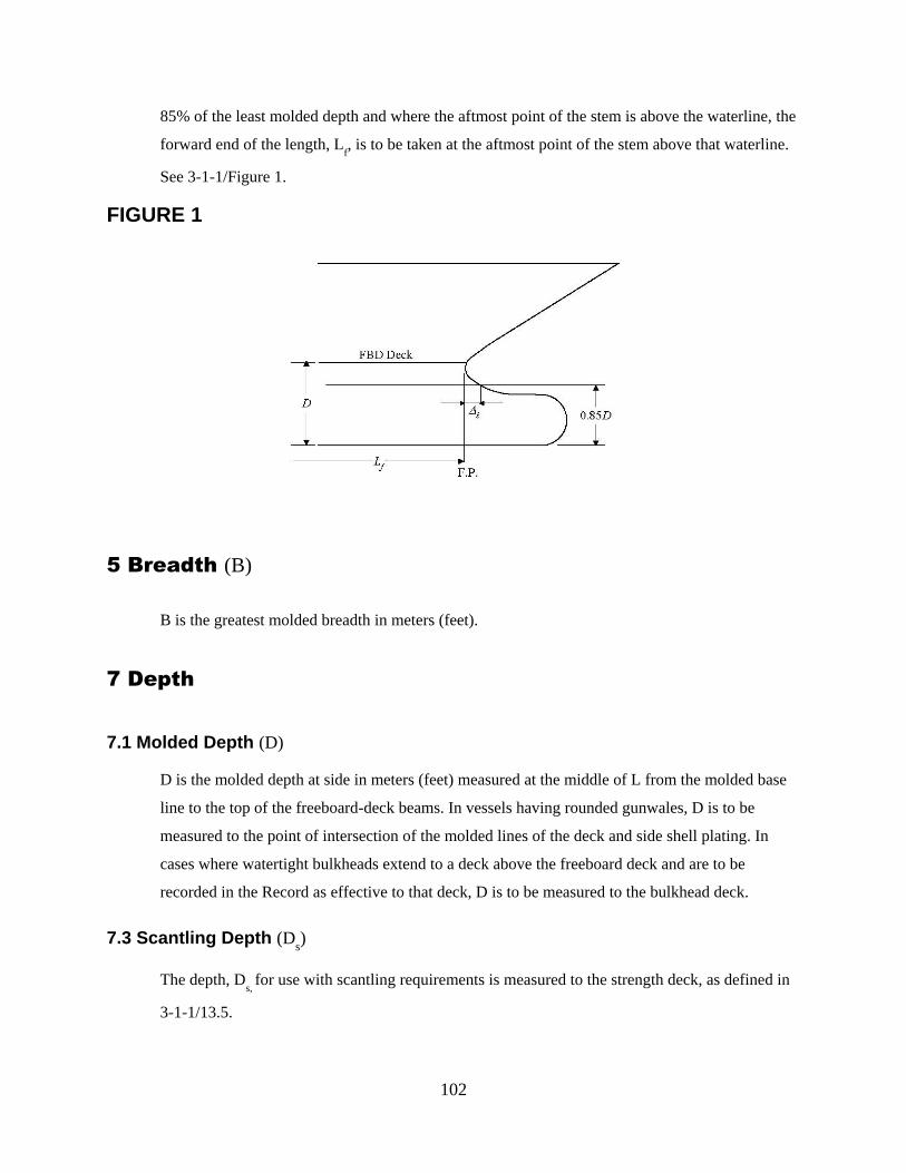
102
85% of the least molded depth and where the aftmost point of the stem is above the waterline, the
forward end of the length, Lf, is to be taken at the aftmost point of the stem above that waterline.
See 3-1-1/Figure 1.
FIGURE 1
5 Breadth (B)
B is the greatest molded breadth in meters (feet).
7 Depth
7.1 Molded Depth (D)
D is the molded depth at side in meters (feet) measured at the middle of L from the molded base
line to the top of the freeboard-deck beams. In vessels having rounded gunwales, D is to be
measured to the point of intersection of the molded lines of the deck and side shell plating. In
cases where watertight bulkheads extend to a deck above the freeboard deck and are to be
recorded in the Record as effective to that deck, D is to be measured to the bulkhead deck.
7.3 Scantling Depth (Ds)
The depth, Ds,
for use with scantling requirements is measured to the strength deck, as defined in
3-1-1/13.5.
103
9 Draft for Scantlings (d)
d is the draft in meters (feet) measured at the middle of the length, L, from the molded keel or the
rabbet line at its lowest point to the estimated summer load waterline, the design load waterline or
0.66D, whichever is greater.
11 Molded Displacement and Block Coefficient
11.1 Molded Displacement (Δ)
Δ is the molded displacement of the vessel in metric tons (long tons), excluding appendages,
taken at the summer load line.
11.3 Block Coefficient (Cb)
Cb is the block coefficient obtained from the following equation:
Cb = Δ/1.025LB
wld (SI & MKS units)
Cb = 35Δ/LB
wld (US units)
where
Δ = molded displacement, as defined in 3-1-1/11.1
L = scantling length, as defined in 3-1-1/3.1
d = draft, as defined in 3-1-1/9
Bwl
= the greatest molded breadth at summer load line
Part 3 Hull Construction and Equipment Chapter 1 General Section 1 Definitions 3-1-1
13 Decks
13.1 Freeboard Deck
The freeboard deck is normally the uppermost continuous deck having permanent means for
closing all openings in its weather portions, and below which all openings in the vessel’s side are
equipped with permanent means for watertight closure. In cases where a vessel is designed for a

104
special draft considerably less than that corresponding to the least freeboard obtainable under the
International Load Line Regulations, the freeboard deck for the purpose of the Rules may be
taken as the lowest actual deck from which the draft can be obtained under those regulations.
13.3 Bulkhead Deck
The bulkhead deck is the highest deck to which watertight bulkheads extend and are made
effective.
13.5 Strength Deck
The strength deck is the deck which forms the top of the effective hull girder at any part of its
length. See Section 3-2-1.
13.7 Superstructure Deck
A superstructure deck is a deck above the freeboard deck to which the side shell plating extends.
Except where otherwise specified, the term superstructure deck, where used in the Rules, refers to
the first such deck above the freeboard deck.
13.9 Deckhouses
A deckhouse is an enclosed structure above the freeboard deck having side plating set inboard of
the hull’s side-shell plating more than 4% of the breadth, B, of the vessel.
15 Deadweight and Lightship Weight
For the purpose of these Rules, the deadweight, DWT, is the difference in metric tons (long tons)
between the displacement of the vessel in water having a specific gravity of 1.025 at the summer
load line and the lightship weight. For the purpose of these Rules, lightship weight is the
displacement of a vessel in metric tons (long tons) without cargo, fuel, lubricating oil, ballast
water, fresh water and feed water in tanks, consumable stores, and passengers and crews and their
effects.
17 Gross Tonnage
17.1 International Tonnage

105
For the purpose of application of these Rules to vessels intended for unrestricted service (see 1-1-
3/1), the referenced gross tonnage throughout the Rules is the measure of the internal volume of
spaces within the vessel as determined in accordance with the provisions of the “International
Convention on Tonnage Measurement of Ships, 1969”.
17.3 National Tonnage
As an alternative to 3-1-1/17.1 above, requirements applicable on the basis of National Tonnage
measurement and National Regulations will be considered for vessels whose operation is intended
to be restricted exclusively to domestic service. (See 1-1-3/7).
3
CHAPTER 2 Hull Structures and Arrangements
SECTION 1 Longitudinal Strength
1 General
Vessels are to have longitudinal hull girder section modulus in accordance with the requirements of this
section. The equation in this section is, in general, valid for all vessels having breadths, B, which do not
exceed two times their depths, D, as defined in Section 3-1-1. Vessels whose proportions exceed these
limits will be subject to special consideration.
3 Longitudinal Hull Girder Strength
3.1 Minimum Section Modulus

106
The minimum required hull girder section modulus, SM, at amidships, is to be determined in accordance
with the following equation:
SM = C1C
2L
2
B (Cb + 0.7) m-cm
2
(ft-in2
)
where
C1
= 30.67 – 0.98L 12 ≤L < 18 m
= 22.40 – 0.52L 18 ≤L < 24 m
= 15.20 – 0.22L 24 ≤L < 35 m
= 11.35 – 0.11L 35 ≤L < 45 m
= 6.40 45 ≤L < 61 m
= 0.0451L + 3.65 61 ≤L < 90 m
C1
= 30.67 – 0.299L 40 ≤L < 59 ft
= 22.40 – 0.158L 59 ≤L < 79 ft
= 15.20 – 0.067L 79 ≤L < 115 ft
= 11.35 – 0.033L 115 ≤L < 150 ft
= 6.40 150 ≤L < 200 ft
= 0.0137L + 3.65 200 ≤L < 295 ft
C2 = 0.01 (0.01, 0.000144)
L = length of vessel, as defined in 3-1-1/3, in m (ft) B = breadth of vessel, as defined in 3-1-1/5, in m (ft)
Cb = block coefficient at design draft, based on the length, L, measured on the design
load waterline. Cb is not to be taken as less than 0.60.

107
5 Decks
5.1 Strength Decks
The uppermost deck to which the side shell plating extends for any part of the length of the vessel is to be
considered the strength deck for that portion of the length, except in way of comparatively short
superstructures. In such a case, the deck on which the superstructures are located is to be considered the
strength deck in way of the superstructure. In general, the effective sectional area of the deck for use in
calculating the section modulus is to exclude hatchways and other large openings through the deck but
may include seam overlaps.
The deck sectional areas used in the section modulus calculations are to be maintained throughout the
midship 0.4L in vessels. They may be reduced to one-half the normal requirement at 0.15L from the ends.
In way of a superstructure beyond the midship 0.4L, the strength deck area may be reduced to
approximately 70% of the normal requirement at that location.
5.3 Effective Lower Decks
To be considered effective for use in calculating the hull girder section modulus, the thickness of the deck
plating is to comply with the requirements of Section 3-2-3. The sectional areas of lower decks used in
calculating the section modulus are to be obtained as described in 3-2-1/5.1. These areas are to be
maintained throughout the midship 0.4L and may be gradually reduced to one-half their midship value at
0.15L from the ends.
7 Longitudinal Strength with Higher-Strength Materials
7.1 General
Vessels in which the effective longitudinal material of either the upper or lower flanges of the main hull
girder, or both, are constructed of materials having mechanical properties greater than those of ordinary
strength hull structural steel [see Section 2-1-2 of the ABS Rules for Materials and Welding (Part 2)], are
to have longitudinal strength generally in accordance with the preceding paragraphs of this section, but
the value of the hull girder section modulus may be modified as permitted by the following paragraphs.
Applications of higher-strength material are to be continuous over the length of the vessel to locations
where the stress levels will be suitable for the adjacent mild steel structure. Higher strength steel is to be
108
extended to suitable locations below the strength deck and above the bottom, so that the stress levels will
be satisfactory for the remaining ordinary strength steel structure. The strength deck and bottom structure
are to be longitudinally framed. The longitudinal framing members are to be essentially of the same
material as the plating they support and are to be continuous throughout the required extent of higher
strength steel. Calculations showing that adequate strength has been provided against buckling are to be
submitted for review and care is to be exercised against the adoption of reduced thicknesses of materials
which may be subject to damage during normal operations.
7.3 Hull Girder Moment of Inertia
The hull-girder moment of inertia is to be not less than required by 3-2-1/3.5.
7.5 Hull Girder Section Modulus
When either the top or the bottom flange of the hull girder, or both, is constructed of higher-strength
material, the section modulus, as obtained from 3-2-1/3.1 or 3-2-1/3.3.4, may be reduced by the factor
Q.
SMhts = Q(SM)
where
Q = 0.78 for Grade H32
Q = 0.72 for Grade H36
H32, H36 are as specified in Section 2-1-3 of the ABS Rules for Materials and Welding (Part 2).
Q factor for steels having other yield point or yield strength will be specially considered.
9 Loading Guidance (1 July 1998)
9.1 Loading Manual and Loading Instrument
All vessels that are contracted for construction on or after July 1998 are to be provided with a loading
manual and, where required, a loading instrument, in accordance with Appendix 3-2-A1.
9.3 Allowable Stresses
9.3.1 At Sea
See 3-2-1/3.3.4 for bending stress and 3-2-1/3.3.5 for shear stress for vessels with ordinary strength steel

109
material. For higher strength steel, the allowable stress may be increased by a factor of 1/Q where Q is as
defined in 3-2-1/7.5.
9.3.2 In Port
The allowable in-port stress is 13.13 kN/cm2
(1.34 tf/cm2
, 8.5 Ltf/in2
) for bending and 10 kN/cm2
(1.025
tf/cm2
, 6.5 Ltf/in2
) for shear. For higher strength steel, the allowable stress may be increased by a factor of
1/Q where Q is as defined in 3-2-1/7.5.
11 Section Modulus Calculation
11.1 Items Included in the Calculation
In general, the following items may be included in the calculation of the section modulus, provided they
are continuous or effectively developed within midship, 0.4L, and gradually tapered beyond the midship,
0.4L. Where the scantlings are based on the still-water bending moment envelope curves, items included
in the hull girder section modulus amidships are to be extended as necessary to meet the hull girder
section modulus required at the location being considered.
Deck plating (strength deck and other effective decks)
Shell and inner bottom plating
Deck and bottom girders
Plating and longitudinal stiffeners of longitudinal bulkheads
All longitudinals of deck, sides, bottom and inner bottom
Continuous longitudinal hatch coamings. See 3-2-1/13.
11.3 Effective Areas Included in the Calculation
In general, the net sectional areas of longitudinal strength members are to be used in the hull girder
section modulus calculations, except that small isolated openings need not be deducted, provided the
openings and the shadow area breadths of the other openings in any one transverse section do not reduce
the section modulus by more than 3%. The breadth or depth of such openings is not to be greater than
1200 mm (47 in.) or 25% of the breadth or depth of the member in which it is located, whichever is less,
with a maximum of 75 mm (3 in.) for scallops. The length of small isolated openings not required to be
deducted is generally not to be greater than 2500 mm (100 in.) The shadow area of an opening is the area
forward and aft of the opening enclosed by the lines tangential to the corners of the opening intersecting
110
each other to form an included angle of 30 degrees.
11.5 Section Modulus to the Deck or Bottom
The section modulus to the deck or bottom is obtained by dividing the moment of inertia by the distance
from the neutral axis to the molded deck at side amidships or baseline, respectively.
11.7 Section Modulus to the Top of Hatch Coamings
For continuous longitudinal hatch coamings, in accordance with 3-2-1/13, the section modulus to the top
of the coaming is to be obtained by dividing the moment of inertia by the distance from the neutral axis to
the deck at side plus the coaming height. This distance need not exceed yt, as given by the following
equation, provided yt is not less than the distance to the molded deck line at side.
yt = y (0.9 + 0.2x/B) m (ft)
where
y = distance, in m (ft), from the neutral axis to the top of the continuous coaming
x = distance, in m (ft), from the top of the continuous coaming to the centerline of the vessel
B = breadth of the vessel, as defined in 3-1-1/5, in m (ft). x and y are to be measured to the point giving
the largest value of yt.
Section modulus to the top of longitudinal hatch coamings between multi-hatchways will be subject to
special consideration.
13 Continuous Longitudinal Hatch Coamings and Above-
Deck Girders
Where strength deck longitudinal coamings of length greater than 0.14L are effectively supported by
longitudinal bulkheads or deep girders, the coamings are to be longitudinally stiffened, in accordance with
3-2-12/7.7. The section modulus amidships to the top of the coaming is to be as required by 3-2-1/3.1, 3-
2-1/3.3, and 3-2-1/11.7, but the section modulus to the deck at side, excluding the coaming, need not be
determined in way of such coaming.
Continuous longitudinal girders on top of the strength deck are to be similarly considered. Their
scantlings are also to be in accordance with Section 3-2-6.

111
3
CHAPTER 2 Hull Structures and Arrangements
SECTION 2 Shell Plating
1 General
Shell plating is to be of not less thickness than is required by the equations for thickness of side and
bottom plating as required by this section, nor less than required by Section 3-2-1 for longitudinal
strength and Section 3-2-8 for deep tank plating with h not less than the vertical distance to the freeboard
deck at side.
3 Bottom Shell Plating
3.1 Extent of Bottom Plating
The term “bottom plating” refers to the plating from the keel to the upper turn of the bilge or upper chine.
3.3 Bottom Shell Plating
The thickness of the bottom shell plating throughout is not to be less than that obtained from the
following equations:
3.3.1
t = /254+ 2.5 mm
t = /460 + 0.10 in.
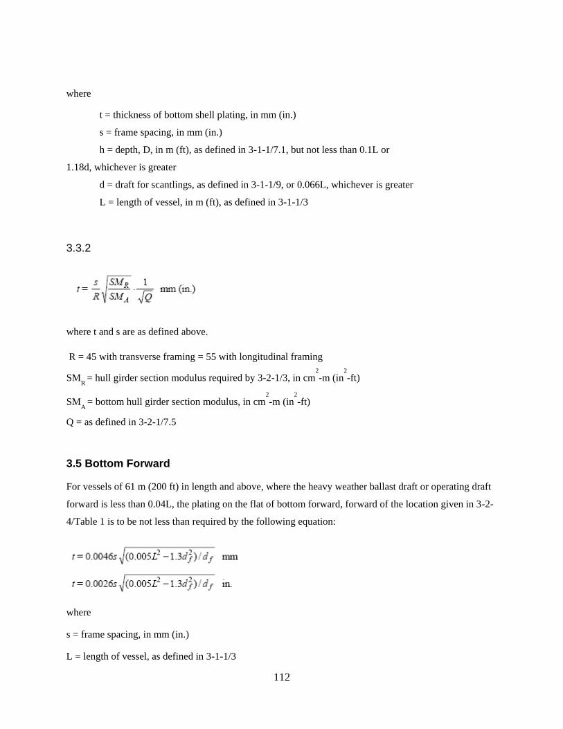
112
where
t = thickness of bottom shell plating, in mm (in.)
s = frame spacing, in mm (in.)
h = depth, D, in m (ft), as defined in 3-1-1/7.1, but not less than 0.1L or
1.18d, whichever is greater
d = draft for scantlings, as defined in 3-1-1/9, or 0.066L, whichever is greater
L = length of vessel, in m (ft), as defined in 3-1-1/3
3.3.2
where t and s are as defined above.
R = 45 with transverse framing = 55 with longitudinal framing
SMR
= hull girder section modulus required by 3-2-1/3, in cm2
-m (in2
-ft)
SMA
= bottom hull girder section modulus, in cm2
-m (in2
-ft)
Q = as defined in 3-2-1/7.5
3.5 Bottom Forward
For vessels of 61 m (200 ft) in length and above, where the heavy weather ballast draft or operating draft
forward is less than 0.04L, the plating on the flat of bottom forward, forward of the location given in 3-2-
4/Table 1 is to be not less than required by the following equation:
where
s = frame spacing, in mm (in.)
L = length of vessel, as defined in 3-1-1/3
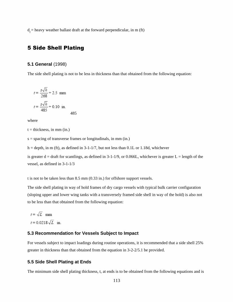
113
df = heavy weather ballast draft at the forward perpendicular, in m (ft)
5 Side Shell Plating
5.1 General (1998)
The side shell plating is not to be less in thickness than that obtained from the following equation:
485
where
t = thickness, in mm (in.)
s = spacing of transverse frames or longitudinals, in mm (in.)
h = depth, in m (ft), as defined in 3-1-1/7, but not less than 0.1L or 1.18d, whichever
is greater d = draft for scantlings, as defined in 3-1-1/9, or 0.066L, whichever is greater L = length of the
vessel, as defined in 3-1-1/3
t is not to be taken less than 8.5 mm (0.33 in.) for offshore support vessels.
The side shell plating in way of hold frames of dry cargo vessels with typical bulk carrier configuration
(sloping upper and lower wing tanks with a transversely framed side shell in way of the hold) is also not
to be less than that obtained from the following equation:
5.3 Recommendation for Vessels Subject to Impact
For vessels subject to impact loadings during routine operations, it is recommended that a side shell 25%
greater in thickness than that obtained from the equation in 3-2-2/5.1 be provided.
5.5 Side Shell Plating at Ends
The minimum side shell plating thickness, t, at ends is to be obtained from the following equations and is
114
not to extend for more than 0.1L from the ends. Between the midship 0.4L and the end 0.1L, the thickness
of the plating may be gradually tapered.
t = 0.0455L + 0.009s mm t = 0.000545L + 0.009s in.
where
s = frame spacing, in mm (in.)
L = length of vessel, as defined in 3-1-1/3, in m (ft)
Where the strength deck at the ends is above the freeboard deck, the thickness of the side plating above
the freeboard deck may be reduced to the thickness given for forecastle and poop sides at the forward and
after ends, respectively.
5.7 Forecastle and Poop Side Plating
5.7.1 Forecastle Side Plating
The thickness, t, of the plating is to be not less than that obtained from the following equation:
t = 0.038(L + 30.8) + 0.006s mm
t = 0.00045(L + 103.3) + 0.006s in.
5.7.2 Poop Side Plating
The thickness, t, of the plating is to be not less than that obtained from the following equation:
t = 0.0296(L + 39.5) + 0.006s mm
t = 0.00035(L + 132.9) + 0.006s in.
where
s = spacing of frames, in mm (in.)
L = length of vessel, as defined in 3-1-1/3, in m (ft)
17 Higher-strength Materials
17.1 General
In general, applications of higher-strength materials are to take into consideration the suitable extension
of the higher-strength material above and below the bottom and deck, respectively, as required by 3-2-
1/7.1. Care is to be taken against the adoption of reduced thickness of material that might be subject to
damage during normal operation. The thickness of bottom and side-shell plating, where constructed of
higher-strength materials, are to be not less than required for purposes of longitudinal hull girder strength;

115
nor are they to be less than required by the foregoing paragraphs of this section when modified as
indicated by the following paragraphs.
17.3 Bottom Plating of Higher-strength Material
Bottom shell plating, where constructed of higher-strength material and where longitudinally framed, is to
be not less in thickness than that obtained from the following equation:
where
thts
= thickness of higher-strength material, in mm (in.)
tms
= thickness, in mm (in.), of ordinary-strength steel, as required by preceding paragraphs of this
section, or from the requirements of other sections of the Rules, appropriate to the vessel type.
C = 4.3 mm (0.17 in.)
Q = as defined in 3-2-1/7.5
17.5 Side Plating of Higher-strength Material
Side-shell plating, where constructed of higher-strength material, is to be not less in thickness than that
obtained from the following equation:
where thts
, tms
, C and Q are as defined in 3-2-2/17.3 for bottom plating.
17.7 End Plating
End-plating thickness, including plating on the flat of bottom forward, where constructed of higher-
strength materials, will be subject to special consideration.

116
3
CHAPTER 2 Hull Structures and Arrangements
SECTION 3 Deck Plating
1 General
The thickness of the deck plating is not to be less than that required to obtain the hull-girder section
modulus given in Section 3-2-1, nor less than required by this section.
3 Deck Plating
The thickness of plating on each deck is to be not less than the greater of those obtained from the
following equations. The required thickness is not to be less than 5.0 mm (0.20 in.), except for platform
decks in enclosed passenger spaces where the thickness is not to be less than 4.5 mm
(0.18 in.). Thickness of strength deck inside line of openings may be reduced by 1.0 mm (0.04 in.) from t
obtained by 3-2-3/3.3 below.
3.1 All Decks
where
t = thickness, in mm (in.)
s = beam or longitudinal spacing, in mm (in.)
h = height, in m (ft), as follows:

117
=for a deck or portion of deck forming a tank top, the greater of the following distances:
two-thirds of the distance from the tank top to the top of the overflow, or
two-thirds of the distance from the tank top to the bulkhead deck or freeboard deck.
=for a lower deck on which cargo or stores are carried, the tween-deck height at side; where the
cargo weights are greater than normal [7010 N/m3
(715 kgf/m3
, 45 lbf/ft3
)], h is to be suitably adjusted.
=for an exposed deck on which cargo is carried, 3.66 m (12 ft). Where it is intended to carry deck
cargoes in excess of 25850 N/m2
(2636 kgf/m2
, 540 lbf/ft2
), this head is to be increased in proportion to the
added loads which will be imposed on the structure
Elsewhere, the value of h is to be not less than that obtained from the appropriate equation below, where
L is the length of vessel in m (ft), as defined in 3-1-1/3.
3.1.1 Exposed Freeboard Deck Having No Deck Below
h = 0.028L + 1.08 m
h = 0.028L + 3.57 ft
3.1.2 Exposed Freeboard Deck Having a Deck Below, Forecastle Deck, Superstructure Deck
Forward of Amidships 0.5L
h = 0.028L + 0.66 m
h = 0.028L + 2.14 ft
3.1.3 Freeboard Deck within Superstructure, Any Deck Below Freeboard Deck, Superstructure
Deck Between 0.25L Forward of and 0.20L Aft of Amidships
h = 0.014L + 0.87 m
h = 0.014L + 2.86 ft
3.1.4 All Other Locations
h = 0.014L + 0.43 m
h = 0.014L + 1.43 ft
3.3 Strength Decks within the Midship 0.8L (2002)
For vessels of length equal to or greater than 61 meters, the strength deck plating within the midship 0.8L

118
shall meet the following requirement: t = 0.009s + 2.4 mm t = 0.009s + 0.095 in. where s = beam or
longitudinal spacing, in mm (in.)
3.5 All Strength Deck Plating Outside the Line of Openings and Other Effective
Deck Plating (2002)
For vessels of length equal to or greater than 61 meters, the strength deck plating within the midship 0.8L
shall meet the following requirement:
where
t = thickness, in mm (in.)
s = beam or longitudinal spacing, in mm (in.), not to be taken less than 610 mm (24 in.)
R = 60 for longitudinal framing, 45 for transverse framing
SMR
= hull girder section modulus required in 3-2-1/3, in cm2
-m (in2
-ft)
SMA
= hull girder section modulus, in cm2
-m (in2
-ft), measured to the deck in question
Q =material factor for the material used in determining SMR, as defined in 3-2-1/7.5
5 Compensation
Compensation is to be provided for openings in the strength deck and other effective decks to maintain
the longitudinal and transverse strength. Openings in the strength deck are to have a minimum corner
radius of 0.125 times the width of the opening, but need not exceed a radius of 600 mm (24 in.). In other
decks, the radius is to be 0.09375 times the width of the opening, but need not exceed radius of 450 mm
(18 in.). Openings are to be a suitable distance from the deck edge, from cargo hatch covers, from
superstructure breaks and from other areas of structural discontinuity.
9 Higher-strength Material
9.1 Thickness
In general, applications of higher strength materials are to take into consideration the suitable extension of
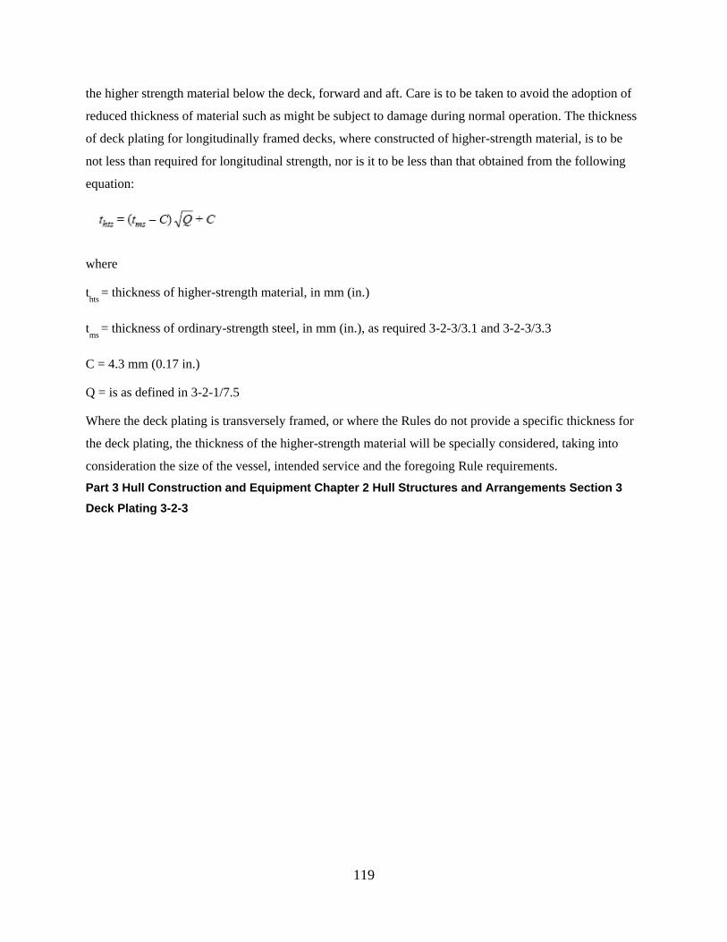
119
the higher strength material below the deck, forward and aft. Care is to be taken to avoid the adoption of
reduced thickness of material such as might be subject to damage during normal operation. The thickness
of deck plating for longitudinally framed decks, where constructed of higher-strength material, is to be
not less than required for longitudinal strength, nor is it to be less than that obtained from the following
equation:
where
thts
= thickness of higher-strength material, in mm (in.)
tms
= thickness of ordinary-strength steel, in mm (in.), as required 3-2-3/3.1 and 3-2-3/3.3
C = 4.3 mm (0.17 in.)
Q = is as defined in 3-2-1/7.5
Where the deck plating is transversely framed, or where the Rules do not provide a specific thickness for
the deck plating, the thickness of the higher-strength material will be specially considered, taking into
consideration the size of the vessel, intended service and the foregoing Rule requirements.
Part 3 Hull Construction and Equipment Chapter 2 Hull Structures and Arrangements Section 3
Deck Plating 3-2-3
120
PART
3
CHAPTER 2 Hull Structures and Arrangements
SECTION 4 Bottom Structure
1 Double Bottoms
1.1 General
Inner bottoms are to be fitted fore and aft between the peaks or as near thereto as practicable in vessels of
ordinary design of 500 GT or over. Where, for special reasons, it may be desired to omit the inner bottom,
the arrangements are to be clearly indicated on the plans when first submitted for approval. A double
bottom need not be fitted in way of deep tanks, provided the safety of the vessel in the event of bottom
damage is not thereby impaired. It is recommended that the inner bottom be arranged to protect the bilges
as much as possible and that it be extended to the sides of the vessel.
Shell longitudinals and frames in way of deep tanks are to have not less strength than is required for
stiffeners on deep tank bulkheads.
1.3 Center Girder
A center girder is to be fitted extending as far forward and aft as practicable. The plates are to be
continuous within the midship three-quarters length; elsewhere, they may be intercostal between floors.
Where double bottoms are to be used for fuel oil or fresh water, the girders are to be intact, but need not
be tested under pressure. This requirement may be modified in narrow tanks at the ends of the vessel or
where other intact longitudinal divisions are provided at about 0.25B from centerline. Where the girders
are not required to be intact, manholes may be cut in every frame space outside the midships three-
quarters length; they may be cut in alternate frames spaces within the midships three-quarters length. For
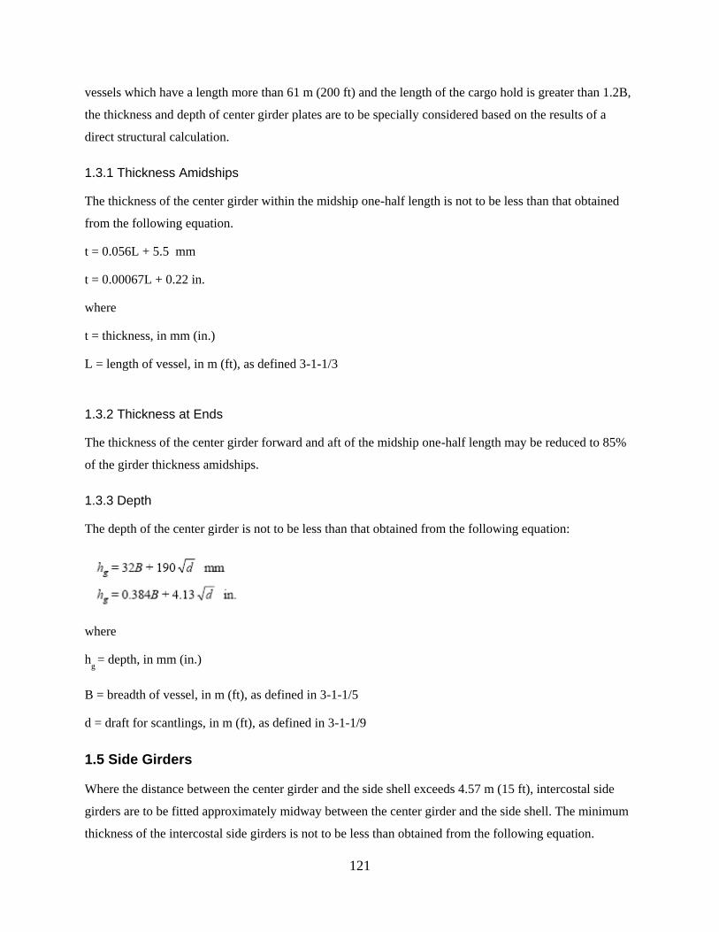
121
vessels which have a length more than 61 m (200 ft) and the length of the cargo hold is greater than 1.2B,
the thickness and depth of center girder plates are to be specially considered based on the results of a
direct structural calculation.
1.3.1 Thickness Amidships
The thickness of the center girder within the midship one-half length is not to be less than that obtained
from the following equation.
t = 0.056L + 5.5 mm
t = 0.00067L + 0.22 in.
where
t = thickness, in mm (in.)
L = length of vessel, in m (ft), as defined 3-1-1/3
1.3.2 Thickness at Ends
The thickness of the center girder forward and aft of the midship one-half length may be reduced to 85%
of the girder thickness amidships.
1.3.3 Depth
The depth of the center girder is not to be less than that obtained from the following equation:
where
hg = depth, in mm (in.)
B = breadth of vessel, in m (ft), as defined in 3-1-1/5
d = draft for scantlings, in m (ft), as defined in 3-1-1/9
1.5 Side Girders
Where the distance between the center girder and the side shell exceeds 4.57 m (15 ft), intercostal side
girders are to be fitted approximately midway between the center girder and the side shell. The minimum
thickness of the intercostal side girders is not to be less than obtained from the following equation.
122
t = 0.036L + c mm
t = 0.00043L + c in.
where
t = thickness, in mm (in.)
L = length of vessel, in m (ft), as defined in 3-1-1/3
c = 4.7 mm (0.18 in.)
1.7 Floors
Solid floors are to be fitted at every frame under the engine room, at every frame in the peaks and under
transverse bulkheads. Elsewhere, the solid floors are to have a maximum spacing of 3.66 m (12 ft) in
association with intermediate open floors or longitudinal framing. The thickness of solid floors is to be
equal to the thickness of side girders obtained in 3-2-4/1.5, except that for widely spaced floors in
association with longitudinal framing, c is to be taken as 6.2 mm (0.24 in.).
1.9 Frames
In transversely framed vessels, open floors consisting of frames and reverse frames are to be fitted at all
frames where solid floors are not fitted. Center and side brackets are to overlap the frames and reverse
frames for a distance equal to 0.05B. They are to be of the thickness required for side girders in the same
location and are to be flanged on their outer edges. Alternatively, longitudinal framing is to be fitted in
association with widely spaced floors. The section modulus, SM, of each frame, reverse frame or bottom,
or inner bottom longitudinal in association with the plating to which it is attached is not to be less than
that obtained from the following equation.
SM = 7.8chs2
cm3
SM = 0.0041chs2
in3
where
s = frame spacing, in m (ft)
= unsupported span between supporting members, in m (ft).
Where brackets are fitted in accordance with 3-1-2/5.5 and are supported by bulkheads, inner bottom, or
side shell, the length, , may be measured as permitted therein.
123
h = vertical distance, in m (ft), from the middle of to the deck at side. In way of a deep tank, h is the
greatest distance from the middle of to a point located at two-thirds of the distance from the top of the
tank to the top of the overflow; a point located above the top of the tank not less than 0.01L + 0.15 m or
0.46 m (0.01L + 0.5 ft or 1.5 ft), whichever is greatest. c for transverse frames and reverse frames: = 0.8
clear of tanks = 1.0 in way of tanks = 0.5 with struts c for longitudinal frames: = 1.0 without struts = 0.55
with struts c for inner bottom longitudinals: = 0.85 without struts = 0.45 with struts Frames and reverse
frames in way of tanks are not to be less than that required clear of tanks if that be greater.
1.11 Struts
Struts are to be angle bar sections fitted midway between floors. In general, they are not to be used where
cargo is discharged by grabs, where heavy cargoes are carried or in the bottom forward slamming area.
The permissible load, Wa, for struts is to be determined in accordance with 3-2-6/3.5.3. The calculated
load, W, is to be determined by:
W = nphs kN (tf, Ltf)
where n = 10.5 (1.07, 0.03)
p = the sum of the half lengths, in m (ft), on each side of the strut, of the frames supported
h = as defined in 3-2-4/1.9
s = frame spacing, in m (ft)
Struts are to be positioned so as to divide the span into approximately equal intervals.
1.13 Inner-bottom Plating
The thickness of the inner-bottom plating throughout the length of the vessel is to be not less than that
obtained from the following equation. Where applicable, the plating is to meet deep tank requirements.
t = 0.037L + 0.009s + c mm
t = 0.000445L + 0.009s + c in.
where
t = thickness, in mm (in.)
L = length of vessel, in m (ft), as defined in 3-1-1/3
s = frame spacing, in mm (in.)
c = 1.5 mm (0.06 in.) in engine space
= −0.5 mm (−0.02 in.) elsewhere

124
Where no ceiling is fitted under cargo hatchways, except for vessels intended for the exclusive carriage of
containers on the inner bottom, the thickness of the inner-bottom plating is to be increased
2.0 mm (0.08 in.). For vessels with longitudinally-framed inner bottoms, the minimum thickness of inner-
bottom plating may be reduced by 1 mm (0.04 in.).
For vessels regularly engaged in trades where the cargo is handled by grabs or similar mechanical
appliances, it is recommended that flush inner-bottom plating be adopted throughout the cargo space, and
that the plating be suitably increased, but the increase need not exceed 5 mm (0.20 in.). It is also
recommended that the minimum thickness be not less than 12.5 mm with 610 mm (0.50 in. with 24 in.)
frame spacing and 19 mm with 915 mm (0.74 in. with 36 in.) frame spacing. Intermediate thicknesses
may be obtained by interpolation.
Where provision is to be made for the operation or stowage of vehicles having rubber tires, and after all
other requirements are met, the thickness of the inner bottom plating is to be not less than that obtained
from 3-2-3/7.
Margin plates which are approximately horizontal are to have thicknesses not less than the adjacent inner
bottom plating. Where they are nearly vertical, they are to be not less than the required inner bottom
plating in the engine space and are to extend the full depth of the inner bottom.
3 Single Bottoms with Floors and Keelsons
3.1 General
Where double bottom construction is not required by 3-2-4/1.1 or is not applied, single bottom
construction is to be in accordance with 3-2-4/3 or 3-2-4/5, as may be applicable.
Part 3 Hull Construction and Equipment Chapter 2 Hull Structures and Arrangements Section 4
Bottom Structure 3-2-4
3.3 Center Keelsons
Single-bottom vessels are to have center keelsons formed of continuous or intercostal center girder plates
with horizontal top plates. The thickness of the keelson and the area of the horizontal top plate are to be
not less than that obtained from the following equations. Vessels less than 30.5 m (100 ft) in length will
be subject to special consideration. Tapering of the horizontal top plate area at the ends is not normally
considered for vessels less than 30.5 m (100 ft) in length. The keelsons are to extend as far forward and
aft as practicable.

125
3.3.1 Center-girder Plate Thickness Amidships
t = 0.063L + 5 mm
t = 0.00075L + 0.2 in.
3.3.2 Center-girder Plates Thickness at Ends
t = 85% of center keelson thickness amidships
3.3.3 Horizontal Top-plate Area Amidships
A = 0.168L3/2
– 8 cm2
A = 0.0044L3/2
– 1.25 in2
3.3.4 Horizontal Top-Plate Area at Ends [L ≥ 30.5 m (100 ft)]
A = 0.127L3/2
– 1 cm2
A = 0.0033L3/2
– 0.15 in2
where
t = thickness of center-girder plate, in mm (in.)
L = length of vessel, as defined in 3-1-1/3, in m (ft)
A = area of horizontal top plate, in cm2
(in2
)
3.5 Side Keelsons
Side keelsons are to be arranged so that there are not more than 2.13 m (7 ft) from the center keelson to
the inner side keelson, from keelson to keelson and from the outer keelson to the lower turn of bilge.
Forward of the midship one-half length, the spacing of keelsons on the flat of floor is not to exceed 915
mm (36 in.). Side keelsons are to be formed of continuous rider plates on top of the floors. They are to be
connected to the shell plating by intercostal plates. The intercostal plates are to be attached to the floor
plates. In the engine space, the intercostal plates are to be of not less thickness than the center girder
plates. The scantlings of the side keelsons are to be obtained from the following equations but need not
exceed 3-2-4/3.3, if that be less.
3.5.1 Side Keelson and Intercostal Thickness Amidships
t = 0.063L + 4 mm
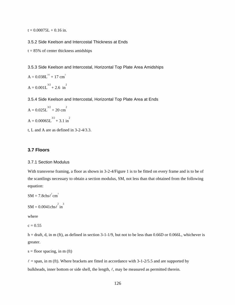
126
t = 0.00075L + 0.16 in.
3.5.2 Side Keelson and Intercostal Thickness at Ends
t = 85% of center thickness amidships
3.5.3 Side Keelson and Intercostal, Horizontal Top Plate Area Amidships
A = 0.038L3/2
+ 17 cm2
A = 0.001L3/2
+ 2.6 in2
3.5.4 Side Keelson and Intercostal, Horizontal Top Plate Area at Ends
A = 0.025L3/2
+ 20 cm2
A = 0.00065L3/2
+ 3.1 in2
t, L and A are as defined in 3-2-4/3.3.
3.7 Floors
3.7.1 Section Modulus
With transverse framing, a floor as shown in 3-2-4/Figure 1 is to be fitted on every frame and is to be of
the scantlings necessary to obtain a section modulus, SM, not less than that obtained from the following
equation:
SM = 7.8chs2
cm3
SM = 0.0041chs2
in3
where
c = 0.55
h = draft, d, in m (ft), as defined in section 3-1-1/9, but not to be less than 0.66D or 0.066L, whichever is
greater.
s = floor spacing, in m (ft)
= span, in m (ft). Where brackets are fitted in accordance with 3-1-2/5.5 and are supported by
bulkheads, inner bottom or side shell, the length, , may be measured as permitted therein.

127
The section modulus may be calculated at the centerline of the vessel, provided the rise of floor is such
that the depth at the toe of brackets is not less than one-half of the depth at the centerline. The above
requirements are limited to cargo holds where cargoes of specific gravity 0.715 or less are uniformly
loaded. In way of engine room and in the forward 0.2L, the floor face bar area is to be doubled.
3.7.2 Depth
The minimum depth of floors at centerline is not be less than that obtained from the following equation:
hf = 62.5l mm
hf = 0.75l in.
where
hf = floor depth, in mm (in.)
= unsupported span of floors, in m (ft). Where brackets are fitted in accordance with 3-1-2/5.5, the
length, , may be measured as permitted therein.
3.7.3 Thickness
The minimum thickness of floors is not to be less than that obtained from the following equation:
t = 0.01hf + 3 mm
t = 0.01hf + 0.12 in.
where
t = floor thickness, in mm (in.)
hf = floor depth, in mm (in.)
Floors under engine girders are to be not less in thickness than the thickness required for keelsons.
FIGURE 1 Plate Floors
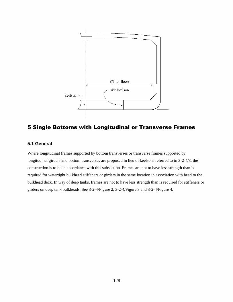
128
5 Single Bottoms with Longitudinal or Transverse Frames
5.1 General
Where longitudinal frames supported by bottom transverses or transverse frames supported by
longitudinal girders and bottom transverses are proposed in lieu of keelsons referred to in 3-2-4/3, the
construction is to be in accordance with this subsection. Frames are not to have less strength than is
required for watertight bulkhead stiffeners or girders in the same location in association with head to the
bulkhead deck. In way of deep tanks, frames are not to have less strength than is required for stiffeners or
girders on deep tank bulkheads. See 3-2-4/Figure 2, 3-2-4/Figure 3 and 3-2-4/Figure 4.

129
FIGURE 2 Round Bottom Floors with Deadrise
FIGURE 3 Transverse Bottom Frames with Longitudinal Side Girders

130
FIGURE 4 Longitudinal Frames with Transverse Webs
5.3 Bottom Girders and Transverses
5.3.1 Section Modulus
The section modulus, SM, of each bottom girder and transverse, where intended as a primary supporting
member, in association with the plating to which it is attached, is not to be less than that obtained from
the following equation:
SM = 7.8chs2
cm3
SM = 0.0041chs2
in3
where
c = 0.915
h = vertical distance, in m (ft), from the center of area supported to the deck at side
s = spacing, in m (ft)
= unsupported span, in m (ft). Where brackets are fitted in accordance with 3-1-2/5.5 and are supported
by bulkheads, inner bottom or side shell, the length, , may be measured as permitted therein.
131
Tripping brackets are to be fitted at intervals of about 3 m (10 ft) and stiffeners are to be fitted as may be
required.
5.3.2 Depth
The minimum depth of the girder or transverse is to be not less than 2.5 times the depth of the cutouts for
bottom frames, unless effective compensation for cutouts is provided, nor less than that obtained from the
following equation:
hw = 145l mm
hw = 1.75l in.
where
hw
= girder or transverse depth, in mm (in.)
is defined in 3-2-4/5.3.1.
5.3.3 Thickness
The minimum thickness of the web is to be not less than that obtained from the following equation:
t = 0.01hw + 3 mm
t = 0.01hw
+ 0.12 in.
where
t = floor thickness, in mm (in.)
hw is as given in 3-2-4/5.3.2.
5.3.4 Non-prismatic Members
Where the cross sectional properties of the member is not constant throughout the length of the girders or
transverses, the above requirements will be specially considered with particular attention being paid to the
shearing forces at the ends.
5.5 Center Girder
In general, a center girder is to be fitted, complying with 3-2-4/5.3; however, alternative arrangements
that provide suitable support for docking will be considered.

132
5.7 Frames
The section modulus, SM, of each bottom frame to the chine or upper turn of bilge, in association with
the plating to which it is attached, is not to be less than that obtained from the following equation:
SM = 7.8chs2
cm3
SM = 0.0041chs2
in3
where
c = 0.80 for transverse frames clear of tanks
= 1.00 for longitudinal frames clear of tanks, and in way of tanks
= 1.00 for transverse frames in way of tanks
s = frame spacing in, m (ft)
= unsupported span, in m (ft), Where brackets are fitted in accordance with 3-1-2/5.5 and are supported
by bulkheads, inner bottom or side shell, the length, , may be measured as permitted therein.
h = vertical distance, in m (ft), from the middle of to the deck at side. In way of a deep tank, h is the
greatest of the distances, in m (ft), from the middle of to a point located at two-thirds of the distance
from the top of the tank to the top of the overflow, a point located above the top of the tank not less than
0.01L + 0.15 m (0.01L + 0.5 ft) or 0.46 m (1.5 ft), whichever is greatest.
L is as defined in 3-1-1/3.
9 Higher-strength Materials
9.1 General
In general, applications of higher-strength materials for bottom structures are to meet the requirements of
this section, but may be modified as permitted by the following paragraphs. Care is to be exercised to
avoid the adoption of reduced thickness of material such as might be subject to damage during normal
operation, and calculations are to be submitted to show adequate provision against buckling. Longitudinal
framing members are to be of essentially the same material as the plating they support.
9.3 Inner-bottom Plating
Inner-bottom plating, where constructed of higher-strength material and where longitudinally framed, is
to be not less in thickness than required by 3-2-4/1.13 or for tank top plating as modified by the following
133
equation:
thts
= [tms
– C][(Q + 2 Q )/3] + C
where
thts
= thickness of higher-strength material, in mm (in.)
tms
= thickness of mild steel, as required by 3-2-4/1.13, in mm (in.), increased where required for no
ceiling
C = 3 mm (0.12 in.) or 5 mm (0.20 in.) where the plating is required by 3-2-4/1.13 to be increased for no
ceiling
Q = as defined in 3-2-1/7.5
The thickness of inner-bottom plating, where transversely framed, will be specially considered.
Where cargo is handled by grabs, or similar mechanical appliances, the recommendations of 3-2-4/1.13
are applicable to thts
.
9.5 Bottom and Inner-bottom Longitudinals
The section modulus of bottom and inner-bottom longitudinals, where constructed of higher-strength
material and in association with the higher-strength plating to which they are attached, are to be
determined as indicated in 3-2-4/1.9, except that the value may be reduced by the factor Q, as defined in
3-2-1/7.5.
9.7 Center Girders, Side Girders and Floors
Center girders, side girders and floors, where constructed of higher-strength materials, are generally to
comply with the requirements of 3-2-4/1.3, 3-2-4/1.5 or 3-2-4/1.7, but may be modified as permitted by
the following equation:
thts
= [tms
– C][(Q + 2 Q )/3] + C
where
thts
, tms
and C are defined in 3-2-4/9.3.
Q is as defined in 3-2-1/7.5.

134

135
3
CHAPTER 2 Hull Structures and Arrangements
SECTION 5 Side Frames, Webs and Stringers
1 General
1.1 Basic Considerations
Frames or webs and stringers are not to have less strength than is required for watertight bulkhead
stiffeners, or girders, in the same location in association with heads to the bulkhead deck. In way of deep
tanks, frames or webs and stringers are not to have less strength than is required for stiffeners or girders
on deep-tank bulkheads. The calculated section modulus is based upon the intact sections being used.
Where a hole is cut in the flange of any member or a large opening is made in the web of the member, the
net section is to be used in determining the section modulus of the member in association with the plating
to which it is attached.
1.3 End Connections
At the ends of unbracketed frames, both the web and the flange are to be welded to the supporting
member. At bracketed end connections, continuity of strength is to be maintained at the connection to the
bracket and at the connection of the bracket to the supporting member. Welding is to be in accordance
with 3-2-16/Table 1. Where longitudinal frames are not continuous at bulkheads, end connections are to
effectively develop their sectional area and resistance to bending. Where a structural member is
terminated, structural continuity is to be maintained by suitable back-up structure, fitted in way of the end
connection of frames, or the end connection is to be effectively extended by a bracket or flat bar to an
adjacent beam, stiffener, etc.
136
3 Longitudinal Side Frames
3.1 Section Modulus
The section modulus, SM, of each longitudinal side frame above the chine or upper turn of bilge is to be
not less than that obtained from the following equation:
SM = 7.8chs2
cm3
SM = 0.0041chs2
in3
where
c = 0.915
h = vertical distance, in m (ft), from the frame to the freeboard deck at side, but not less than 0.02L + 0.46
m (0.02L + 1.5 ft)
s = frame spacing, in m (ft)
= straight-line unsupported span, in m (ft). Where brackets are fitted in accordance with 3-1-2/5.5 and
are supported by bulkheads, the length, , may be measured as permitted therein.
5 Transverse Side Frames
5.1 Section Modulus
The section modulus, SM, of each transverse side frame other than tween deck frames above the chine or
upper turn of bilge, in association with the plating to which the frame is attached, is not to be less than
that obtained from the following equation. See 3-2-5/Figure 1, 3-2-5/Figure 2 and 3-2-5/Figure 3.
SM = 7.8chs2
cm3
SM = 0.0041chs2
in3
where
c = 0.915 for frames having no tween decks above
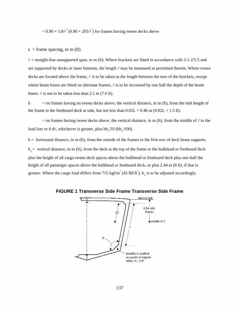
137
= 0.90 + 5.8/3
(0.90 + 205/3
) for frames having tween decks above
s = frame spacing, in m (ft)
= straight-line unsupported span, in m (ft). Where brackets are fitted in accordance with 3-1-2/5.5 and
are supported by decks or inner bottoms, the length may be measured as permitted therein. Where tween
decks are located above the frame, is to be taken as the length between the toes of the brackets, except
where beam knees are fitted on alternate frames, is to be increased by one half the depth of the beam
knees. is not to be taken less than 2.1 m (7.0 ft).
h = on frames having no tween decks above, the vertical distance, in m (ft), from the mid length of
the frame to the freeboard deck at side, but not less than 0.02L + 0.46 m (0.02L + 1.5 ft).
= on frames having tween decks above, the vertical distance, in m (ft), from the middle of to the
load line or 0.4, whichever is greater, plus bh1/33 (bh
1/100).
b = horizontal distance, in m (ft), from the outside of the frames to the first row of deck beam supports.
h1 = vertical distance, in m (ft), from the deck at the top of the frame to the bulkhead or freeboard deck
plus the height of all cargo tween deck spaces above the bulkhead or freeboard deck plus one-half the
height of all passenger spaces above the bulkhead or freeboard deck, or plus 2.44 m (8 ft), if that is
greater. Where the cargo load differs from 715 kgf/m3
(45 lbf/ft3
), h1 is to be adjusted accordingly.
FIGURE 1 Transverse Side Frame Transverse Side Frame

138
FIGURE 2
FIGURE 3 Hold and Tween Deck Frames
5.3 Tween-deck Frames
The section modulus, SM, of each transverse side frame above the chine or upper turn of bilge, in
association with the plating to which the frame is attached, is not to be less than obtained from the
following equation:

139
SM = 7.8chs2
cm3
SM = 0.0041chs2
in3
where
c = 0.90
h = 0.032L – 0.68 m (0.032L – 2.23 ft) type A frame
= 0.049L – 0.81 m (0.049L – 2.66 ft) type B frame
= 0.052L – 0.13 m (0.052L – 0.43 ft) type C frame
= in no case less than the vertical distance, in m (ft), from the mid-length of the frame to the
freeboard deck, but not less than 0.02L + 0.46 m (0.02L + 1.5 ft)
s = frame spacing, in m (ft)
= tween deck height or unsupported length along frame, whichever is greater, in m (ft), not to be taken
less than 2.13 m (7.0 ft). For frame types, see 3-2-5/Figure 3. Forward of 0.125L, frames above the
bulkhead or freeboard deck are to be type B frames.
Longitudinal tween deck frames are to meet the requirements of 3-2-5/3. The section modulus of each
longitudinal tween deck frame forward of 0.125L from the stem is to be not less than required by 3-2-
5/5.1 for transverse frames in the same location, taking as the unsupported span along the frame length.
7 Side Web Frames
7.1 Section Modulus
The section modulus, SM, of each side web frame supporting longitudinal framing or shell stringers
above the chine or upper turn of bilge, in association with the plating to which the web frame is attached,
is not to be less than that obtained from the following equation:
SM = 7.8chs2
cm3
SM = 0.0041chs2
in3
where

140
c = 0.915 aft of the forepeak
= 1.13 in the forepeak of vessel 61 m (200 ft) or greater in length.
s = frame spacing, in m (ft)
= straight-line unsupported span, in m (ft). Where brackets are fitted in accordance with 3-1-2/5.5 and
are supported by decks or inner bottoms, the length, , may be measured as permitted therein
h = on frames having no tween decks above, the vertical distance, in m (ft), from the mid length of
the frame to the freeboard deck at side, but not less than 0.02L + 0.46 m (0.02L + 1.5 ft).
= on frames having tween decks above, the vertical distance, in m (ft), from the middle of to the
load line or 0.5, whichever is greater, plus bh1/45K (bh
1/150K).
b = horizontal distance, in m (ft), from the outside of the frames to the first row of deck beams supports.
h1 = vertical distance, in m (ft), from the deck at the top of the web frame to the bulkhead or freeboard
deck plus the height of all cargo tween deck spaces above the bulkhead or freeboard deck plus one-half
the height of all passenger spaces above the bulkhead or freeboard deck, or plus 2.44 m (8 ft), if that is
greater. Where the cargo load differs from 715 kgf/m3
(45 lbf/ft3
), h1 is to be adjusted accordingly.
K = 1.0 where the deck is longitudinally framed and a deck transverse is fitted in way of each web
frame.
= the number of transverse frame spaces between web frames where the deck is transversely
framed.
7.3 Tween-deck Web Frames
Tween-deck web frames are to be fitted below the bulkhead deck over the hold web frames, as may be
required to provide continuity of transverse strength above the main web frames in holds and machinery
space.
141
7.5 Proportions
The depth of each web frame is to be not less than 125 mm (1.5 in.) or, unless effective compensation is
provided for cutouts, 2.5 times the cutout for frame or longitudinal if greater. The thickness of the web of
web frame or stringer is to be not less than 0.01 times the depth plus 3 mm (0.12 in.), is as defined in 3-
2-5/7.1.
9 Recommendation for Vessels Subject to Impact
For vessels subject to impact loadings during routines, it is recommended that side frames with a section
modulus 25% greater than that obtained above be provided.
11 Side Stringers
11.1 Section Modulus
The section modulus, SM, of each side stringer in association with the plating to which the side stringer is
attached is not to be less than that obtained from the following equation:
SM = 7.8chs2
cm3
SM = 0.0041chs2
in3
where
c = 0.915
= 1.13 in the forepeak of vessel 61 m (200 ft) or greater in length.
h = vertical distance, in m (ft), from the middle of s to the freeboard deck at side, but not less than
0.02L + 0.46 m (0.02L + 1.5 ft).
= for stringers above the lowest deck or at a similar height in relation to the design draft, not less
than given in 3-2-5/5.3 appropriate to the tween deck location.
= for stringers in the peaks of vessels 61 m (200 ft) or greater in length, not less than given in 3-2-
5/5.5.
s = sum of the half lengths, in m (ft), (on each side of the stringer) of the frames supported.
= span, in m (ft), between web frames, or between web frame and bulkhead. Where brackets are fitted

142
in accordance with 3-1-2/5.5 and are supported by transverse bulkheads, the length, , may be measured
as permitted therein.
11.3 Proportions
Side stringers are to have a depth of not less than 0.125 (1.5 in per ft of span ) plus one-quarter of the
depth of the slot for the frames, but need not exceed the depth of the web frames to which they are
attached. In general, the depth is not to be less than 2.5 times the depth of the slots, or the slots are to be
fitted with filler plates. The thickness of each stringer is to be not less than 0.014L + 7.2 mm (0.00017L +
0.28 in.) where L is as defined in 3-1-1/3.

143
APPENDIX B – Global Variable Description
There are two global variables in PCAT: USER which holds the user inputs, and HULL which
holds the details of each specific variant, both are structures. Because there is more than one
variant HULL is set up as a matrix, where the first dimension is the variant number, and the
second dimension is the run number. Each of the two variables are structures with multiple
fields. They are described in detail below.
Matlab is a case sensitive code, and in PCAT, HULL and USER are capitalized to bring attention
to these global variables. Most of the rest of the variables and fields are in lowercase. To aide a
person in editing the code, all variables discussed in this thesis are capitalized in the same
manner as in PCAT.
Name: USER.geometry
Data type: structure
Purpose: Stores user information from the geometry screen.
Name: USER.geometry.length
Data type: array
Purpose: Stores an array of user specified lengths. Lengths are stored in meters.
Example: [30 35 40]
Name: USER.geometry.ltob
Data type: array
Purpose: Stores an array of user specified rations of length to beams. Ratios are non-
dimensional.
Example: [4.5 5.2]
Name: USER.geometry.ltod
Data type: array
144
Purpose: Stores an array of user specified rations of length to depths at midships. Ratios are non-
dimensional.
Example: [7 7.5 8.15]
Name: USER.geometry.ph
Data type: cell holding a string or strings
Purpose: Stores a name of the parent hull.
Example: {'NPL High Speed Round Bilge' 'PC-14'}
Name: USER.geometry.dh
Data type: array
Purpose: Stores an array of user specified deck heights. Deck height is stored in meters.
Example: [2.5]
Name: USER.loading
Data type: structure
Purpose: Stores user information from the loading screen.
Name: USER.loading.kgtod
Data type: array
Purpose: Stores an array of user specified ratios of the center of gravity to depth at midships.
Ratios are non-dimensional.
Example: [0.6]
Name: USER.loading.lcg
Data type: array or string
Purpose: Stores an array of user specified ratios of the longitudinal center of gravity to the length
between perpendiculars. Ratios are non-dimensional. When set to 'd', PCAT will set the
LCG to the default value of the longitudinal center of buoyancy (LCB) if the LCG falls
between the values of -0.02 and -0.13 If it does not, LCG is set to the nearest valid value

145
(either -0.02 or -0.13). Note that HULL.loading.lcg will never be reset from 'd', the LCG is
set in the variable HULL for the particular variant.
Example: 'd'
Name: USER.loading.materials
Data type: cell holding a string or strings
Purpose: Stores the name of the material types to be used.
Example: {'Ordinary Strength Steel' 'AH-32'}
Name: USER.loading.fs
Data type: array
Purpose: Stores an array of user specified frame spacing values. Frame spacing is stored in
meters.
Example: [1.4 1.5 1.6]
Name: USER.machinery
Data type: structure
Purpose: Stores user information from the machinery and manning screen relevant to machinery.
Name: USER.machinery.eps
Data type: array
Purpose: Stores an array of user specified number of engines per shaft. All engines on board will
be the same type (there are no secondary engines). Only possible values are [1] and [1 2]
corresponding to only 1 engine per shaft or either 1 or 2 engines per shaft.
Example: [1]
Name: USER.machinery.shafts
Data type: array
Purpose: Stores an array of user specified number of shafts.
Example: [2 4]

146
Name: USER.machinery.wj
Data type: structure
Purpose: Stores user a 1 if water jets are going to be analyzed, a 0 if wj will not be analyzed.
Name: USER.machinery.prop
Data type: structure
Purpose: Stores user a 1 if propellers are going to be analyzed, a 0 if propellers will not be
analyzed.
Name: USER.manning
Data type: structure
Purpose: Stores user information from the machinery and manning screen relevant to manning.
Name: USER.manning.officer
Data type: scalar
Purpose: Stores the percentage of total manning that is officers.
Example: [.15]
Name: USER.manning.cpo
Data type: scalar
Purpose: Stores the percentage of total manning that is chief petty officers.
Example: [.15]
Name: USER.manning.enlisted
Data type: scalar
Purpose: Stores the percentage of total manning that is junior enlisted.
Example: [.70]
Name: USER.manning.total
Data type: array
Purpose: Stores an array of user specified manning levels.

147
Example: [15 20 25]
Name: USER.speed
Data type: structure
Purpose: Stores user information from the speed screen relevant to machinery.
Name: USER.speed.profile_speed
Data type: array
Purpose: Stores an array the array of containing the speeds entered in the speed profile. The
length of this array is the same as the length of the profile_percent array.
Example: [5 10 12.5 15 20]
Name: USER.speed.profile_percent
Data type: array
Purpose: Stores an array the array of containing the percentages entered in the speed profile.
Element (n) corresponds to the nth element of the profile speed array. This array is the same
as the length of the profile_percent array, and the sum of all the elements is 100.
Example: [20 35 25 15 5]
Name: USER.speed.max
Data type: scalar
Purpose: Stores the user specified maximum speed in knots.
Example: [20]
Name: USER.speed.endurance
Data type: scalar or string
Purpose: Stores the user specified endurance speed in knots. If the user desires the endurance
speed to be set to the most fuel efficient speed, this variable is set to 'd'.
Example: 'd' or [9]
Name: USER.speed.range

148
Data type: array
Purpose: Stores an array of user specified ranges.
Example: [700 800]
Name: USER.weapons
Data type: structure
Purpose: Stores user information from the weapons screen relevant to C4I, weapons, and
navigation equipment. The information in this variable should account for all of the
equipment in SWBS 400, SWBS 700, and the variable ammunition loads.
Name: USER.weapons.id
Data type: cell holding strings
Purpose: Hold identifiers for each weapon set. The length of this variable is equal to the number
of weapon sets.
Example: {'Low' 'Med' 'High'}
Name: USER.weapons.weight
Data type: array
Purpose: Stores the weights for each weapons set in LT. The nth element of this array
corresponds to the nth weapon set.
Example: [5 8 12]
Name: USER.weapons.dharea
Data type: array
Purpose: Stores the required main deck area for each weapons set in m2. The nth element of this
array corresponds to the nth weapon set.
Example: [9 9.5 10]
Name: USER.weapons.iharea
Data type: array

149
Purpose: Stores the required in-hull area for each weapons set in ft2. The nth element of this
array corresponds to the nth weapon set.
Example: [27 27 30]
Name: USER.weapons.power
Data type: array
Purpose: Stores the required electrical power for each weapons set in kW. The nth element of
this array corresponds to the nth weapon set. This value is not used in this version of the
program.
Example: [100 120 170]
Name: USER.weapons.kgtod
Data type: array
Purpose: Stores the ratio of the height of the center of gravity of each weapons set above the keel
over the midship's depth (KG/D). This number is non dimensional. The nth element of this
array corresponds to the nth weapon set. This value is not used in this version of the program.
Example: [1 1.1 0.9]
Name: USER.weapons.wmoe
Data type: array
Purpose: Stores the measure of effectiveness of a given weapons system relative to the users own
standard. Prior to using PCAT, the user must have developed measure of effectiveness for
the weapons systems (wmoe). This can incorporate range of radars or weapons, warhead
size, maintainability, ability to penetrate certain armor, interoperability, or any other way of
comparing systems. The number stored in this variable should be between 0 and 1.
Example: [0.40 0.60 0.90]
Name: USER.weapons.cost
Data type: array
Purpose: Stores the cost of the weapons systems in thousands of dollars. The nth element of this
array corresponds to the nth weapon set.
150
Example: [1100 2500 3000]
Name: USER.omoe
Data type: structure
Purpose: Level one fields (ops, mob, and weps) store the relative importance of the level one
measures of effectiveness. The remaining fields are classified are level two.
The level one fields are: ops (operations), weps (weapons), and mob (mobility). They all hold a
scalar representing the relative importance if the field. Level 1 fields should sum to 1.
The level two fields are:
USER.omoe.speed - maximum speed in kts
USER.omoe.endurance - days at sea
USER.omoe.range - maximum range in nm
USER.omoe.draft – design draft in ft
USER.omoe.md - available main deck space less the main deck space used by the
weapons in ft2.
USER.omoe.ih - available in-hull deck space less the main deck space used by the
weapons and the prime movers (ft2).
USER.omoe.man - manning of the ship created
USER.omoe.sea – %MSI
The level two fields either have a length of 3, in which case the elements are [threshold goal
moe] or a length of one in which case the element is [moe]. If the level two fields have a length
of one the threshold value is set to the worst possible output and the goal value is set to the best
possible output in the course of the program. The first four fields (speed, endurance, range, and
draft) are the mobility parameters. The sum of their moe's should be 1. The last four fields (md,
ih, man, and sea) are the operation parameters. The sum of their moe's should also be 1. It is
important to note that this variable is reassigned during the execution of PCAT so at the
completion of the program, every level two field has a length of three. Therefore if default
values are desired in subsequent runs, the user must specify this in each run.

151
Name: USER.cost
Data type: structure
Purpose: Holds relevant cost information. Each field holds a scalar value of the price of some
aspect of the ship or other relevant cost parameters. The fields are:
manning – price of a man-year in $/man-year
life – estimated life of the hull in years
ops – percent of time the variant is operational in percent
fuel – price of fuel in $/L
Name: USER.sea
Data type: scalar
Purpose: Holds the value of the seastate for seakeeping analysis.
Name: USER.rsm
Data type: binary bscalar
Purpose: Set to 1 if the current run uses response surface modeling.

152
Figure B-0-1 USER variable breakdown
Name: HULL
Data type: structure
Purpose: Stores user information for a particular variant. HULL is sized by NxM, where N is the
variant number and M is the run number. For the remainder of this appendix, HULL(N,M) will
be represented as HULL.
Name: HULL.geometry
Data type: structure
Purpose: Holds relevant geometrical parameters for a particular variant. Fields are all scalars
unless otherwise noted. Fields are:
USER
geometry
length
ltob
ltod
ph
dh
loading
lcg
fs
kgtod
materials
machinery
eps
shafts
wj
prop
manning
officer
cpo
enlisted
total
speed
profile_speed
profile_percent
max
endurance
range
weapons
id
weight
dharea
iharea
power
kgtod
wmoe
cost
omoe
ops
mob
weps
speed
endurance
range
draft
md
ih
man
sea
rsm
cost
OSS
AH32
AH36
engine
manning
life
ops
fuel
sea

153
lbp – length between perpendiculars (m), initially set by the user, but changes as the
design draft of the ship is adjusted.
loa – length overall (m), unlike lbp, this variable is constant for a given hull throughout
the design process.
beam_max – maximum ship beam (m)
depth – midships depth (m)
dh – deck height, or separation of internal decks (m)
ph – cell containing a string that names the parent hull
wsa – wetted surface area (m2), surface area of the wetted portion of the hull at design
draft.
main_deckarea – area of the main deck (m2)
iharea – area of internal decks (m2)
displacement – displacement of the ship at design draft (mton)
beam_wl – beam of the ship at the waterline (m)
Cb – block coefficient, defined as 𝐷𝑖𝑠𝑝𝑙𝑎𝑐𝑒𝑑 𝑉𝑜𝑙𝑢𝑚𝑒
𝐷𝑒𝑠𝑖𝑔𝑛 𝐷𝑟𝑎𝑓𝑡 ∗𝐿𝐵𝑃∗𝐵𝑒𝑎𝑚 𝑎𝑡 𝑤𝑎𝑡𝑒𝑟𝑙𝑖𝑛𝑒
Cp – prismatic coefficient, defined as 𝐷𝑖𝑠𝑝𝑙𝑎𝑐𝑒𝑑 𝑉𝑜𝑙𝑢𝑚𝑒
𝑀𝑎𝑥𝑖𝑚𝑢𝑚 𝑠𝑢𝑏𝑚𝑒𝑟𝑔𝑒𝑑 𝑠𝑒𝑐𝑡𝑖𝑜𝑛 𝑎𝑟𝑒𝑎 ∗𝐿𝐵𝑃
gm – metacentric height (m)
km – height of the metacenter above the keel (m)
draft – design draft (m), initially set by the parent hull selection, but changes as ship is
balanced.
offsets – structure holding offsets of the ship. This is described in more detail below.
Name: HULL.geometry.offsets
Data type: structure
Purpose: Holds the offsets for a ship. The offsets for this program are stored in an
unconventional way to allow for easier processing of the data. This requires the user to ensure
the data is properly formatted before entering a new hull. The offsets are broken into three
coordinates X (longitudinal), Y (transverse), and Z (vertical) with the origin being at the forward
perpendicular, centerline, and baseline respectively. Positive X is aft, positive Y is to port, and
positive Z is upwards. To represent the offsets a grid is placed on the hull in the X-Z plane.
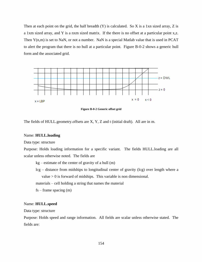
154
Then at each point on the grid, the half breadth (Y) is calculated. So X is a 1xn sized array, Z is
a 1xm sized array, and Y is a nxm sized matrix. If the there is no offset at a particular point x,z.
Then Y(n,m) is set to NaN, or not a number. NaN is a special Matlab value that is used in PCAT
to alert the program that there is no hull at a particular point. Figure B-0-2 shows a generic hull
form and the associated grid.
Figure B-0-2 Generic offset grid
The fields of HULL.geometry.offsets are X, Y, Z and t (initial draft). All are in m.
Name: HULL.loading
Data type: structure
Purpose: Holds loading information for a specific variant. The fields HULL.loading are all
scalar unless otherwise noted. The fields are
kg – estimate of the center of gravity of a hull (m)
lcg – distance from midships to longitudinal center of gravity (lcg) over length where a
value > 0 is forward of midships. This variable is non dimensional.
materials – cell holding a string that names the material
fs – frame spacing (m)
Name: HULL.speed
Data type: structure
Purpose: Holds speed and range information. All fields are scalar unless otherwise stated. The
fields are:

155
profile_speed – an array of speeds at which a variant is analyzed for resistance and fuel
efficiencies. This array begins as the speeds in knots input by the user in the speed
profile but then is "beefed up" to include at speeds in 1 knot increments from a
Froude number of 0.1 to the maximum speed (if Froude number of the maximum
speed is < 1.0).
profile_percent – an array representing the percent of the time a craft spends at a given
speed when operational. This array is initially put in by the user. Zeroes are added
for every speed that is added in the "beef up" process so the length of this array is the
same at the length of profile_speed.
max – maximum speed (knots) input by the user
endurance – endurance speed (knots) or 'd' for default. Either input by the user or
calculated as the most fuel efficient speed.
range – range of the variant in nm. See chapter 3 for more information on range.
new_max – final maximum speed of the hull accounting for the actual engines placed on
board. This number will be greater than the value input by the user.
endurance_days – number of days the ship can stay at sea without refueling at endurance
speed using 2/3 of the available fuel.
Name: HULL.machinery
Data type: structure
Purpose: Holds machinery information relevant to all engineroom machinery. All fields are
scalar unless otherwise stated. The fields are:
eps – engines per shaft, can either be 1 or 2
shafts – number of shafts on this variant
wj – binary variable that equals 1 if waterjets are used and 0 if not
prop - binary variable that equals 1 if waterjets are used and 0 if not
endurance_nm_LT – fuel efficiency at endurance speed in nm per LT
nm_LT – an array the same length as the "beefed up" speed profile. Element (n) of this
field is the fuel efficiency of the ship in nm per LT at a speed equal to
HULL.speed.profile_speed(n).

156
sfc_profile - an array the same length as the "beefed up" speed profile. Element (n) of
this field is the specific fuel consumption of the ship in 𝑙𝑏𝑠 𝑝 ∗ 𝑟 at a speed equal
to HULL.speed.profile_speed(n).
Name: HULL.weapons
Data type: structure
Purpose: Holds the information on the weapons systems input by the user for a particular variant.
The fields are the same as USER.weapons with the exception that each field of HULL.weapons
only holds one value.
Name: HULL.manning
Data type: structure
Purpose: Holds the information on the manning of the variant. The fields are all scalar and in
units of people. The fields are:
officer – number of officers
cpo – number of chief petty officers
enlisted – number of junior enlisted
total – total number of people
Name: HULL.resistance
Data type: structure
Purpose: Holds information or resistance and powering for a particular variant. The fields are all
structures also.
bhehp – bare hull effective horsepower (kW), stores the bare hull EHP of the hull.
ehp – EHP with appendages (kW)
bhp – Brake horsepower, or the power required by the engine to move the ship at a given
speed (kW).
Each of these fields is a structure and has multiple parts. So for example HULL.resistance.bhp
has three fields max, endurance, and profile corresponding to the required power at maximum
speed, endurance speed, and along the speed profile.

157
max – horsepower at user specified maximum speed. This variable is a scalar.
endurance – horsepower at endurance speed. Note this field will not exist for bhehp and
ehp if the user set endurance to default. This variable is a scalar.
profile – power requited along the speed profile. This variable is an array of powers the
same length as the profile_speed.
Name: HULL.good
Data type: scalar
Purpose: This scalar is initially set to 0 and then is change to 1 if the ship converges.
Name: HULL.error
Data type: string
Purpose: This string is the reason for a particular ship not converging.
Name: HULL.engine
Data type: structure
Purpose: Holds information on the propulsion engine selected. HULL.engine has the following
fields:
Model – a string holding the model name
Specs – an array describing the model. The elements of Specs are:
[ID, length(m), width(m), height(m), weight(mton), maximum BHP(kW),
RPM(max)]
SFC – an matrix describing the engine at different rpms. Each row of SFC corresponds
to a different RPM. The first five elements are for the engine used in a non-marine
environemt. The second five elements are for the engine attached to a propeller.
Therefore only the last five elements of each row of SFC were used in PCAT. Each
row has the following elements.
[RPM, BHP, Torque(N-m), SFC (kg/kW-hr), GPH (L/hr), RPM, BHP, Torque, SFC, GPH]
SHP – the final shaft power of the ship.
Name: HULL.temp_weight

158
Data type: structure
Purpose: This structure has fields that hold weights generated outside of the weight module. The
fields are:
F41 – Full load fuel loading (mton)
structures – weight of structures generated in the structures section (mton)
Name: HULL.structures
Data type: structure
Purpose: Holds information relevant to structures of a variant. All fields hold scalars unless
otherwise stated. The fields are:
SM - limiting (minimum) section modulus of the midships section in m-cm2
bsp – bottom shell plating thickness (cm)
ssp_m – side shell plating thickness near midships (cm)
ssp_e – side shell plating thickness near the ends (cm)
dp – array of deck plating thicknesses (cm), element 1 is the main deck, element 2 is the
first deck below the main deck, etc.
x_bg – critical thickness of the bottom girder (cm). See chapter 3 for more information
on critical thicknesses.
x_bf – critical thickness of the bottom frame (cm)
x_sf – critical thickness of the side frame (cm)
x_ss – critical thickness of the side stringers frame (cm)
NA – location of the neutral axis above baseline (m)
Name: HULL.weight
Data type: array of structures
Purpose: HULL.weight is an array with length 10 where each element is a structure.

159
Element of HULL.weight Information stored
HULL.weight(1) Information on SWBS 100
HULL.weight(2) Information on SWBS 200
HULL.weight(3) Information on SWBS 300
HULL.weight(4) Information on SWBS 400 and 700
and various variable loads
HULL.weight(5) Information on SWBS 500
HULL.weight(6) Information on SWBS 600
HULL.weight(7) Only holds naming information
HULL.weight(8) Empty
HULL.weight(9) Information variable loads
HULL.weight(10) Information on the total weight
Figure B-0-3 HULL.weight description
HULL.weight(4) holds information on the weights for SWBS groups 400, SWBS 700 and the
variable ammunition because the user inputs the weights for SWBS 400, SWBS 700 and the
variable ammunition as a group and there is no reason to separate them. HULL.weight(9) holds
the information on the remainder of the variable loads. The fields of each structure are:
groups – scalar that holds the groups weight in mton
SWBS – string that holds the SWBS number
name – string that holds the name of the SWBS group.
Name: HULL.seakeeping
Data type: structure
Purpose: Holds the seakeeping information number for the ship.
Name: HULL.seakeeping.period
Data type: array
Purpose: Holds the array of periods at which the seakeeping analysis was performed. This array
is in seconds.
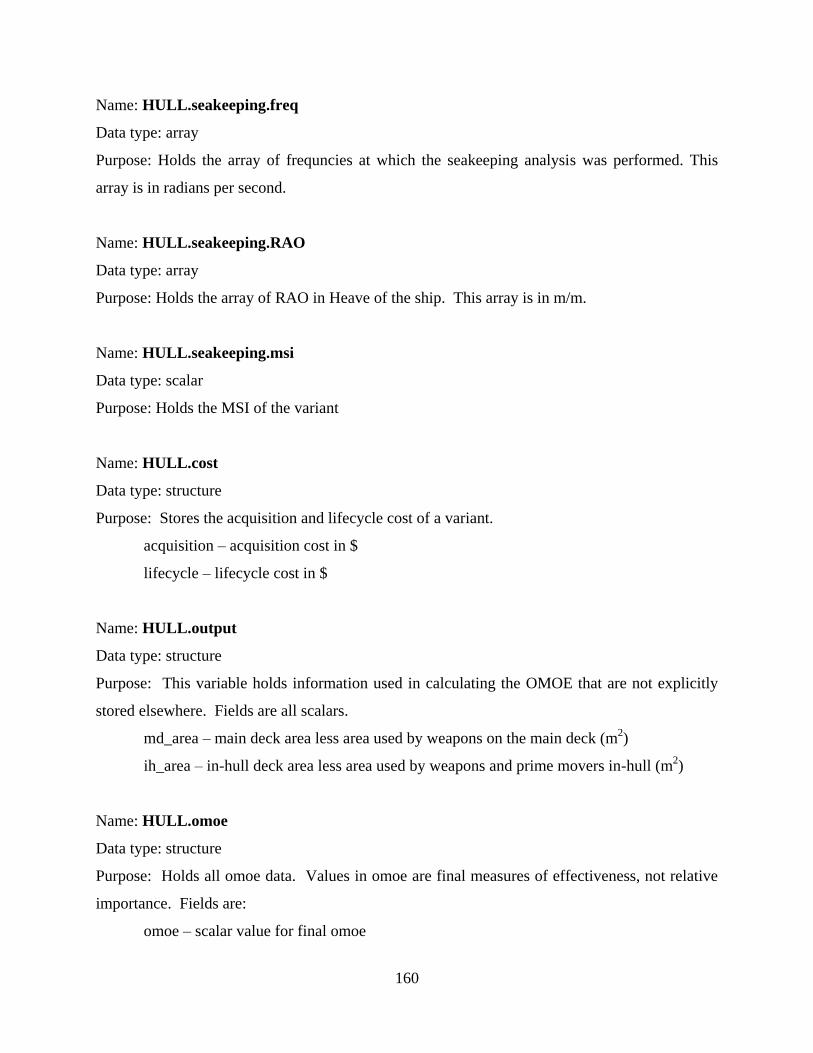
160
Name: HULL.seakeeping.freq
Data type: array
Purpose: Holds the array of frequncies at which the seakeeping analysis was performed. This
array is in radians per second.
Name: HULL.seakeeping.RAO
Data type: array
Purpose: Holds the array of RAO in Heave of the ship. This array is in m/m.
Name: HULL.seakeeping.msi
Data type: scalar
Purpose: Holds the MSI of the variant
Name: HULL.cost
Data type: structure
Purpose: Stores the acquisition and lifecycle cost of a variant.
acquisition – acquisition cost in $
lifecycle – lifecycle cost in $
Name: HULL.output
Data type: structure
Purpose: This variable holds information used in calculating the OMOE that are not explicitly
stored elsewhere. Fields are all scalars.
md_area – main deck area less area used by weapons on the main deck (m2)
ih_area – in-hull deck area less area used by weapons and prime movers in-hull (m2)
Name: HULL.omoe
Data type: structure
Purpose: Holds all omoe data. Values in omoe are final measures of effectiveness, not relative
importance. Fields are:
omoe – scalar value for final omoe

161
moe_1 – array of second tier moe results. First elements are related to mobility. The last
four elements are related to operations. The elements are: [speed, endurance, range,
draft, md_area, ih_area, manning, seakeeping]
mob – scalar value for mobility moe
ops – scalar value for operations moe
weps – scalar value for weapons moe
Figure B-0-4 and Figure B-0-5 show the breakdown of HULL to the second level.
HULL.geometry.offsets and all of the HULL.resistance fields are broken down to the third level
as described above.
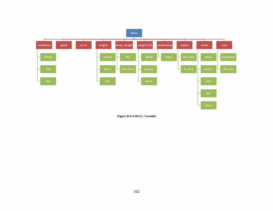
162
Figure B-0-4 HULL Variable
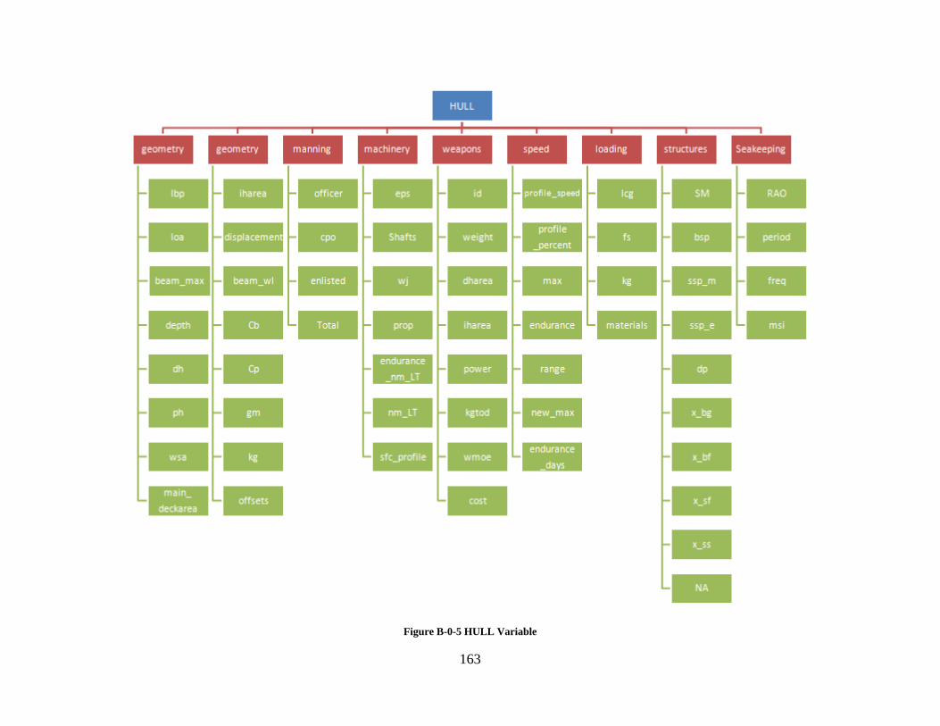
163
Figure B-0-5 HULL Variable
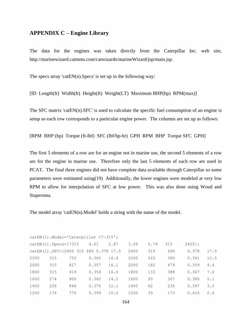
164
APPENDIX C – Engine Library
The data for the engines was taken directly from the Caterpillar Inc. web site,
http://marinewizard.catmms.com/catwizards/marineWizard/jsp/main.jsp.
The specs array 'catEN(n).Specs' is set up in the following way:
[ID Length(ft) Width(ft) Height(ft) Weight(LT) Maximum BHP(hp) RPM(max)]
The SFC matrix 'catEN(n).SFC' is used to calculate the specific fuel consumption of an engine is
setup so each row corresponds to a particular engine power. The columns are set up as follows:
[RPM BHP (hp) Torque (ft-lbf) SFC (lbf/hp-hr) GPH RPM BHP Torque SFC GPH]
The first 5 elements of a row are for an engine not in marine use, the second 5 elements of a row
are for the engine in marine use. Therefore only the last 5 elements of each row are used in
PCAT. The final three engines did not have complete data available through Caterpillar so some
parameters were estimated using(19) Additionally, the lower engines were modeled at very low
RPM to allow for interpolation of SFC at low power. This was also done using Woud and
Stapersma.
The model array 'catEN(n).Model' holds a string with the name of the model.
catEN(1).Model='Caterpillar C7-315';
catEN(1).Specs=[7315 4.01 2.87 3.06 0.79 315 2400];
catEN(1).SFC=[2400 315 689 0.378 17.0 2400 315 690 0.378 17.0
2200 315 752 0.365 16.4 2200 243 580 0.361 12.5
2000 315 827 0.357 16.1 2000 182 479 0.359 9.4
1800 315 919 0.356 16.0 1800 133 388 0.367 7.0
1600 274 900 0.362 14.2 1600 93 307 0.380 5.1
1400 226 848 0.376 12.1 1400 62 235 0.397 3.5
1200 176 770 0.399 10.0 1200 39 173 0.420 2.4

165
1000 127 668 0.432 7.8 1000 23 119 0.449 1.5
1 1 1 0.648 0 1 1 1 0.648 0];
catEN(2).Model='Caterpillar C9-503';
catEN(2).Specs=[9503 3.93 3.15 3.22 0.93 503 2500];
catEN(2).SFC=[2500 503 1056 0.362 26.0 2500 503 1056 0.362 26.0
2400 503 1100 0.357 25.6 2400 445 974 0.362 23.0
2300 503 1148 0.349 25.1 2300 392 894 0.358 20.0
2200 509 1216 0.342 24.9 2200 343 818 0.352 17.2
2100 509 1275 0.338 24.6 2100 298 746 0.347 14.8
1900 508 1404 0.336 24.4 1900 221 610 0.350 11.0
1800 495 1443 0.335 23.7 1800 188 548 0.356 9.5
1700 469 1450 0.335 22.4 1700 158 488 0.361 8.2
1600 436 1430 0.337 21.0 1600 132 433 0.367 6.9
1500 378 1324 0.353 19.0 1500 109 381 0.373 5.8
1300 235 948 0.408 13.7 1300 71 285 0.390 3.9
1100 162 774 0.461 10.7 1100 43 204 0.412 2.5
1000 137 718 0.471 9.2 1000 32 169 0.425 2.0
900 113 657 0.469 7.5 900 23 137 0.442 1.5
800 91 599 0.466 6.1 800 16 108 0.473 1.1
600 58 504 0.478 3.9 600 7 61 0.582 0.6
1 1 1 0.655 0 1 1 1 0.655 0];
catEN(3).Model='Caterpillar C12-660';
catEN(3).Specs=[12660 5.16 3.47 3.30 1.16 660 2300];
catEN(3).SFC=[2300 660 1507 0.362 34.1 2300 660 1507 0.362 34.1
2200 664 1584 0.352 33.4 2200 577 1378 0.347 28.6
2000 661 1735 0.342 32.3 2000 434 1140 0.340 21.1
1800 662 1932 0.343 32.5 1800 316 923 0.344 15.5
1600 661 2170 0.350 33.0 1600 222 729 0.346 11.0
1400 545 2044 0.355 27.7 1400 149 558 0.345 7.3
1200 282 1235 0.356 14.3 1200 94 410 0.363 4.9
1000 172 904 0.353 8.7 1000 54 285 0.419 3.2
600 68 597 0.340 3.3 600 12 103 0.770 1.3
1 1 1 0.862 0 1 1 1 0.862 0];
catEN(4).Model='Caterpillar C15-800';
catEN(4).Specs=[15800 5.01 3.09 3.84 1.44 800 2300];
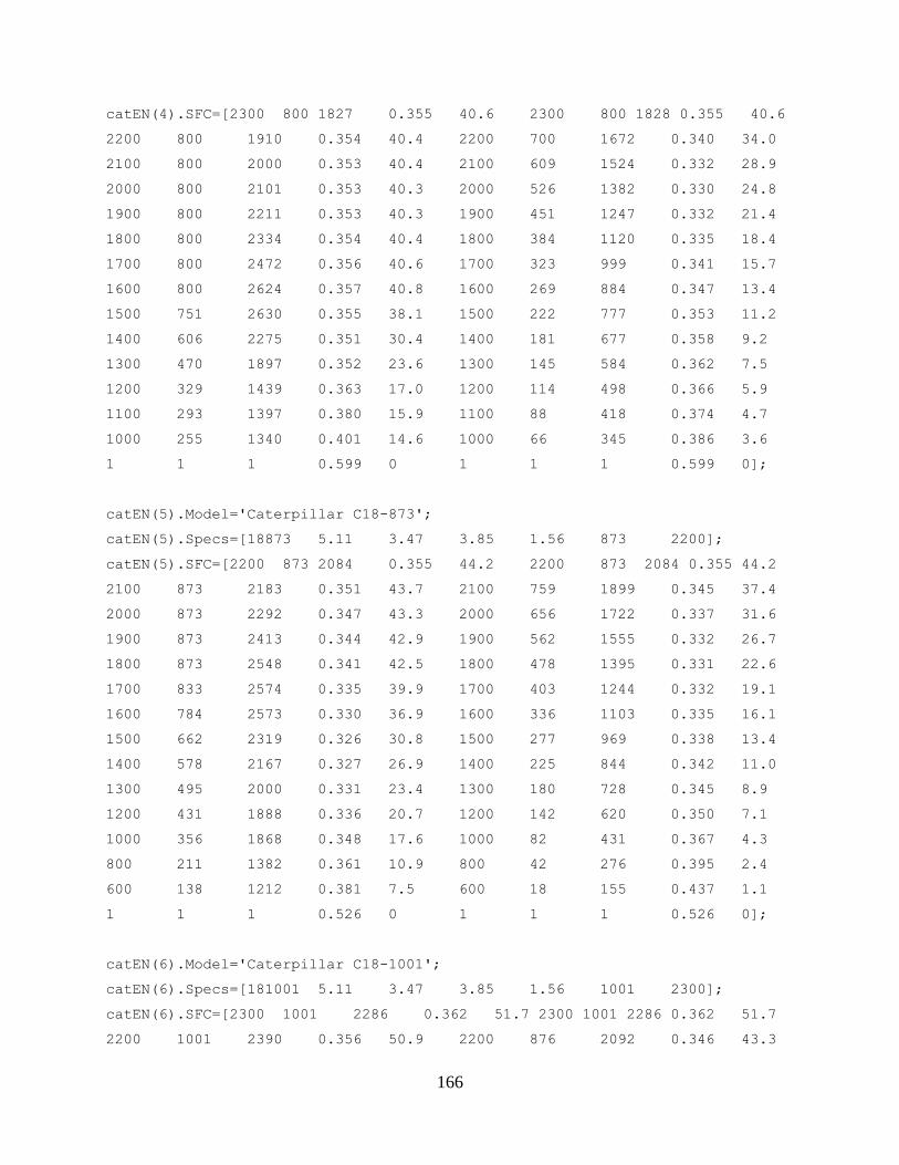
166
catEN(4).SFC=[2300 800 1827 0.355 40.6 2300 800 1828 0.355 40.6
2200 800 1910 0.354 40.4 2200 700 1672 0.340 34.0
2100 800 2000 0.353 40.4 2100 609 1524 0.332 28.9
2000 800 2101 0.353 40.3 2000 526 1382 0.330 24.8
1900 800 2211 0.353 40.3 1900 451 1247 0.332 21.4
1800 800 2334 0.354 40.4 1800 384 1120 0.335 18.4
1700 800 2472 0.356 40.6 1700 323 999 0.341 15.7
1600 800 2624 0.357 40.8 1600 269 884 0.347 13.4
1500 751 2630 0.355 38.1 1500 222 777 0.353 11.2
1400 606 2275 0.351 30.4 1400 181 677 0.358 9.2
1300 470 1897 0.352 23.6 1300 145 584 0.362 7.5
1200 329 1439 0.363 17.0 1200 114 498 0.366 5.9
1100 293 1397 0.380 15.9 1100 88 418 0.374 4.7
1000 255 1340 0.401 14.6 1000 66 345 0.386 3.6
1 1 1 0.599 0 1 1 1 0.599 0];
catEN(5).Model='Caterpillar C18-873';
catEN(5).Specs=[18873 5.11 3.47 3.85 1.56 873 2200];
catEN(5).SFC=[2200 873 2084 0.355 44.2 2200 873 2084 0.355 44.2
2100 873 2183 0.351 43.7 2100 759 1899 0.345 37.4
2000 873 2292 0.347 43.3 2000 656 1722 0.337 31.6
1900 873 2413 0.344 42.9 1900 562 1555 0.332 26.7
1800 873 2548 0.341 42.5 1800 478 1395 0.331 22.6
1700 833 2574 0.335 39.9 1700 403 1244 0.332 19.1
1600 784 2573 0.330 36.9 1600 336 1103 0.335 16.1
1500 662 2319 0.326 30.8 1500 277 969 0.338 13.4
1400 578 2167 0.327 26.9 1400 225 844 0.342 11.0
1300 495 2000 0.331 23.4 1300 180 728 0.345 8.9
1200 431 1888 0.336 20.7 1200 142 620 0.350 7.1
1000 356 1868 0.348 17.6 1000 82 431 0.367 4.3
800 211 1382 0.361 10.9 800 42 276 0.395 2.4
600 138 1212 0.381 7.5 600 18 155 0.437 1.1
1 1 1 0.526 0 1 1 1 0.526 0];
catEN(6).Model='Caterpillar C18-1001';
catEN(6).Specs=[181001 5.11 3.47 3.85 1.56 1001 2300];
catEN(6).SFC=[2300 1001 2286 0.362 51.7 2300 1001 2286 0.362 51.7
2200 1001 2390 0.356 50.9 2200 876 2092 0.346 43.3
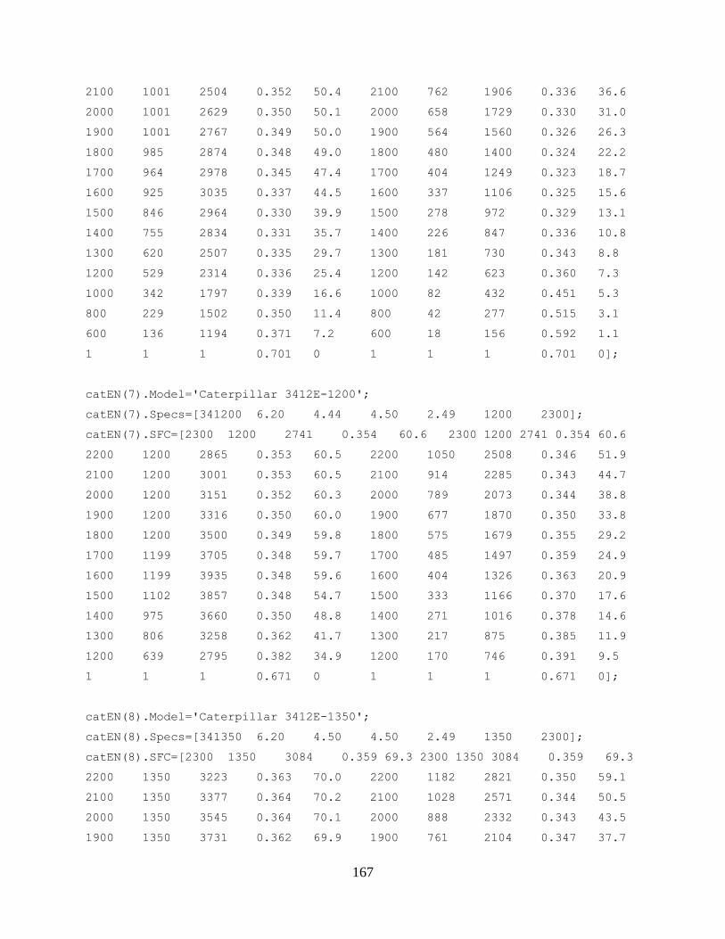
167
2100 1001 2504 0.352 50.4 2100 762 1906 0.336 36.6
2000 1001 2629 0.350 50.1 2000 658 1729 0.330 31.0
1900 1001 2767 0.349 50.0 1900 564 1560 0.326 26.3
1800 985 2874 0.348 49.0 1800 480 1400 0.324 22.2
1700 964 2978 0.345 47.4 1700 404 1249 0.323 18.7
1600 925 3035 0.337 44.5 1600 337 1106 0.325 15.6
1500 846 2964 0.330 39.9 1500 278 972 0.329 13.1
1400 755 2834 0.331 35.7 1400 226 847 0.336 10.8
1300 620 2507 0.335 29.7 1300 181 730 0.343 8.8
1200 529 2314 0.336 25.4 1200 142 623 0.360 7.3
1000 342 1797 0.339 16.6 1000 82 432 0.451 5.3
800 229 1502 0.350 11.4 800 42 277 0.515 3.1
600 136 1194 0.371 7.2 600 18 156 0.592 1.1
1 1 1 0.701 0 1 1 1 0.701 0];
catEN(7).Model='Caterpillar 3412E-1200';
catEN(7).Specs=[341200 6.20 4.44 4.50 2.49 1200 2300];
catEN(7).SFC=[2300 1200 2741 0.354 60.6 2300 1200 2741 0.354 60.6
2200 1200 2865 0.353 60.5 2200 1050 2508 0.346 51.9
2100 1200 3001 0.353 60.5 2100 914 2285 0.343 44.7
2000 1200 3151 0.352 60.3 2000 789 2073 0.344 38.8
1900 1200 3316 0.350 60.0 1900 677 1870 0.350 33.8
1800 1200 3500 0.349 59.8 1800 575 1679 0.355 29.2
1700 1199 3705 0.348 59.7 1700 485 1497 0.359 24.9
1600 1199 3935 0.348 59.6 1600 404 1326 0.363 20.9
1500 1102 3857 0.348 54.7 1500 333 1166 0.370 17.6
1400 975 3660 0.350 48.8 1400 271 1016 0.378 14.6
1300 806 3258 0.362 41.7 1300 217 875 0.385 11.9
1200 639 2795 0.382 34.9 1200 170 746 0.391 9.5
1 1 1 0.671 0 1 1 1 0.671 0];
catEN(8).Model='Caterpillar 3412E-1350';
catEN(8).Specs=[341350 6.20 4.50 4.50 2.49 1350 2300];
catEN(8).SFC=[2300 1350 3084 0.359 69.3 2300 1350 3084 0.359 69.3
2200 1350 3223 0.363 70.0 2200 1182 2821 0.350 59.1
2100 1350 3377 0.364 70.2 2100 1028 2571 0.344 50.5
2000 1350 3545 0.364 70.1 2000 888 2332 0.343 43.5
1900 1350 3731 0.362 69.9 1900 761 2104 0.347 37.7
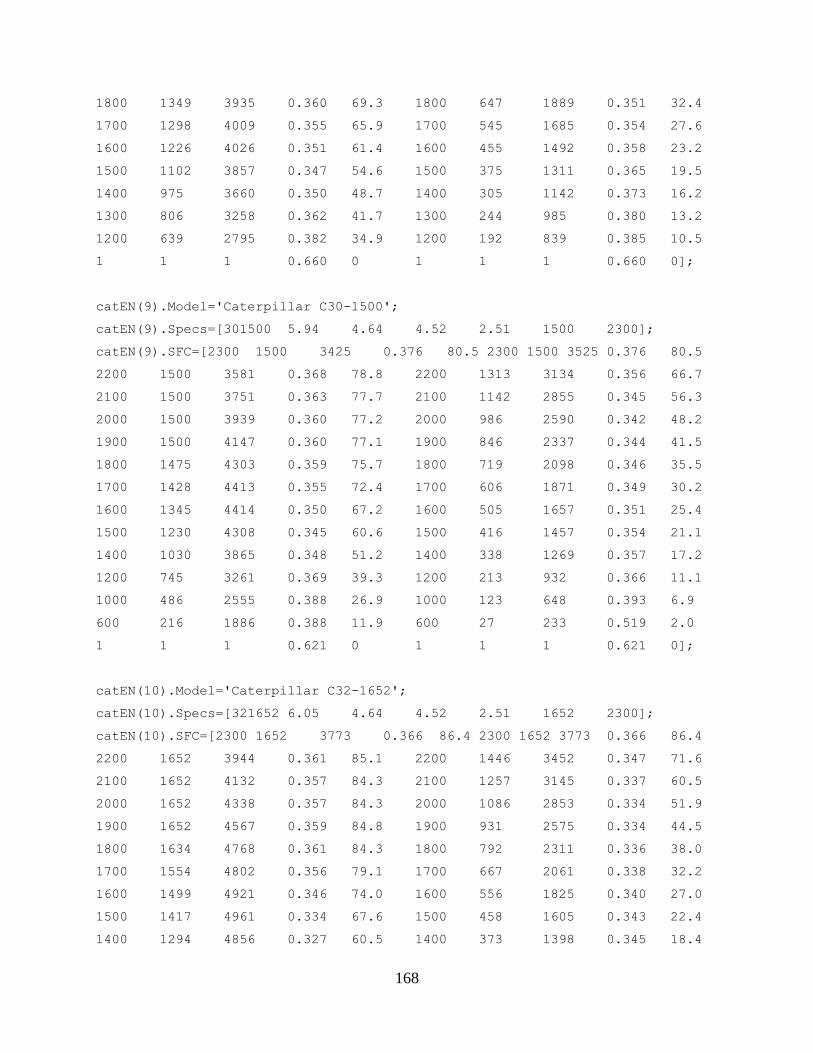
168
1800 1349 3935 0.360 69.3 1800 647 1889 0.351 32.4
1700 1298 4009 0.355 65.9 1700 545 1685 0.354 27.6
1600 1226 4026 0.351 61.4 1600 455 1492 0.358 23.2
1500 1102 3857 0.347 54.6 1500 375 1311 0.365 19.5
1400 975 3660 0.350 48.7 1400 305 1142 0.373 16.2
1300 806 3258 0.362 41.7 1300 244 985 0.380 13.2
1200 639 2795 0.382 34.9 1200 192 839 0.385 10.5
1 1 1 0.660 0 1 1 1 0.660 0];
catEN(9).Model='Caterpillar C30-1500';
catEN(9).Specs=[301500 5.94 4.64 4.52 2.51 1500 2300];
catEN(9).SFC=[2300 1500 3425 0.376 80.5 2300 1500 3525 0.376 80.5
2200 1500 3581 0.368 78.8 2200 1313 3134 0.356 66.7
2100 1500 3751 0.363 77.7 2100 1142 2855 0.345 56.3
2000 1500 3939 0.360 77.2 2000 986 2590 0.342 48.2
1900 1500 4147 0.360 77.1 1900 846 2337 0.344 41.5
1800 1475 4303 0.359 75.7 1800 719 2098 0.346 35.5
1700 1428 4413 0.355 72.4 1700 606 1871 0.349 30.2
1600 1345 4414 0.350 67.2 1600 505 1657 0.351 25.4
1500 1230 4308 0.345 60.6 1500 416 1457 0.354 21.1
1400 1030 3865 0.348 51.2 1400 338 1269 0.357 17.2
1200 745 3261 0.369 39.3 1200 213 932 0.366 11.1
1000 486 2555 0.388 26.9 1000 123 648 0.393 6.9
600 216 1886 0.388 11.9 600 27 233 0.519 2.0
1 1 1 0.621 0 1 1 1 0.621 0];
catEN(10).Model='Caterpillar C32-1652';
catEN(10).Specs=[321652 6.05 4.64 4.52 2.51 1652 2300];
catEN(10).SFC=[2300 1652 3773 0.366 86.4 2300 1652 3773 0.366 86.4
2200 1652 3944 0.361 85.1 2200 1446 3452 0.347 71.6
2100 1652 4132 0.357 84.3 2100 1257 3145 0.337 60.5
2000 1652 4338 0.357 84.3 2000 1086 2853 0.334 51.9
1900 1652 4567 0.359 84.8 1900 931 2575 0.334 44.5
1800 1634 4768 0.361 84.3 1800 792 2311 0.336 38.0
1700 1554 4802 0.356 79.1 1700 667 2061 0.338 32.2
1600 1499 4921 0.346 74.0 1600 556 1825 0.340 27.0
1500 1417 4961 0.334 67.6 1500 458 1605 0.343 22.4
1400 1294 4856 0.327 60.5 1400 373 1398 0.345 18.4
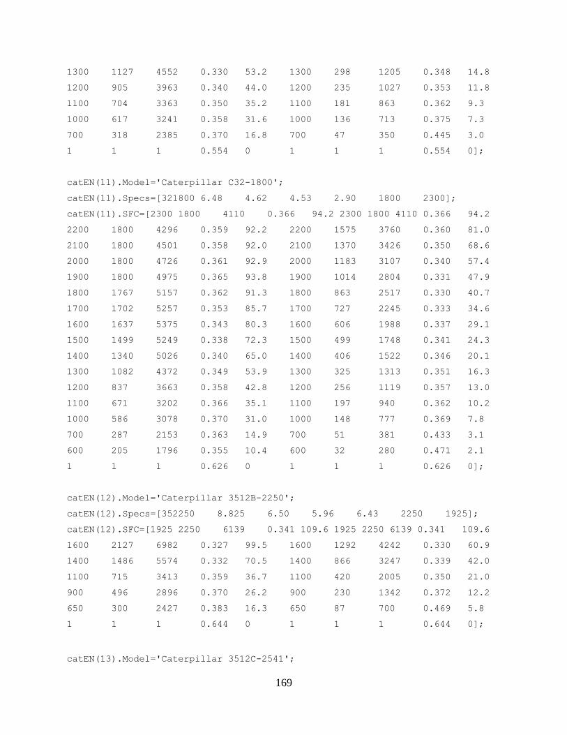
169
1300 1127 4552 0.330 53.2 1300 298 1205 0.348 14.8
1200 905 3963 0.340 44.0 1200 235 1027 0.353 11.8
1100 704 3363 0.350 35.2 1100 181 863 0.362 9.3
1000 617 3241 0.358 31.6 1000 136 713 0.375 7.3
700 318 2385 0.370 16.8 700 47 350 0.445 3.0
1 1 1 0.554 0 1 1 1 0.554 0];
catEN(11).Model='Caterpillar C32-1800';
catEN(11).Specs=[321800 6.48 4.62 4.53 2.90 1800 2300];
catEN(11).SFC=[2300 1800 4110 0.366 94.2 2300 1800 4110 0.366 94.2
2200 1800 4296 0.359 92.2 2200 1575 3760 0.360 81.0
2100 1800 4501 0.358 92.0 2100 1370 3426 0.350 68.6
2000 1800 4726 0.361 92.9 2000 1183 3107 0.340 57.4
1900 1800 4975 0.365 93.8 1900 1014 2804 0.331 47.9
1800 1767 5157 0.362 91.3 1800 863 2517 0.330 40.7
1700 1702 5257 0.353 85.7 1700 727 2245 0.333 34.6
1600 1637 5375 0.343 80.3 1600 606 1988 0.337 29.1
1500 1499 5249 0.338 72.3 1500 499 1748 0.341 24.3
1400 1340 5026 0.340 65.0 1400 406 1522 0.346 20.1
1300 1082 4372 0.349 53.9 1300 325 1313 0.351 16.3
1200 837 3663 0.358 42.8 1200 256 1119 0.357 13.0
1100 671 3202 0.366 35.1 1100 197 940 0.362 10.2
1000 586 3078 0.370 31.0 1000 148 777 0.369 7.8
700 287 2153 0.363 14.9 700 51 381 0.433 3.1
600 205 1796 0.355 10.4 600 32 280 0.471 2.1
1 1 1 0.626 0 1 1 1 0.626 0];
catEN(12).Model='Caterpillar 3512B-2250';
catEN(12).Specs=[352250 8.825 6.50 5.96 6.43 2250 1925];
catEN(12).SFC=[1925 2250 6139 0.341 109.6 1925 2250 6139 0.341 109.6
1600 2127 6982 0.327 99.5 1600 1292 4242 0.330 60.9
1400 1486 5574 0.332 70.5 1400 866 3247 0.339 42.0
1100 715 3413 0.359 36.7 1100 420 2005 0.350 21.0
900 496 2896 0.370 26.2 900 230 1342 0.372 12.2
650 300 2427 0.383 16.3 650 87 700 0.469 5.8
1 1 1 0.644 0 1 1 1 0.644 0];
catEN(13).Model='Caterpillar 3512C-2541';
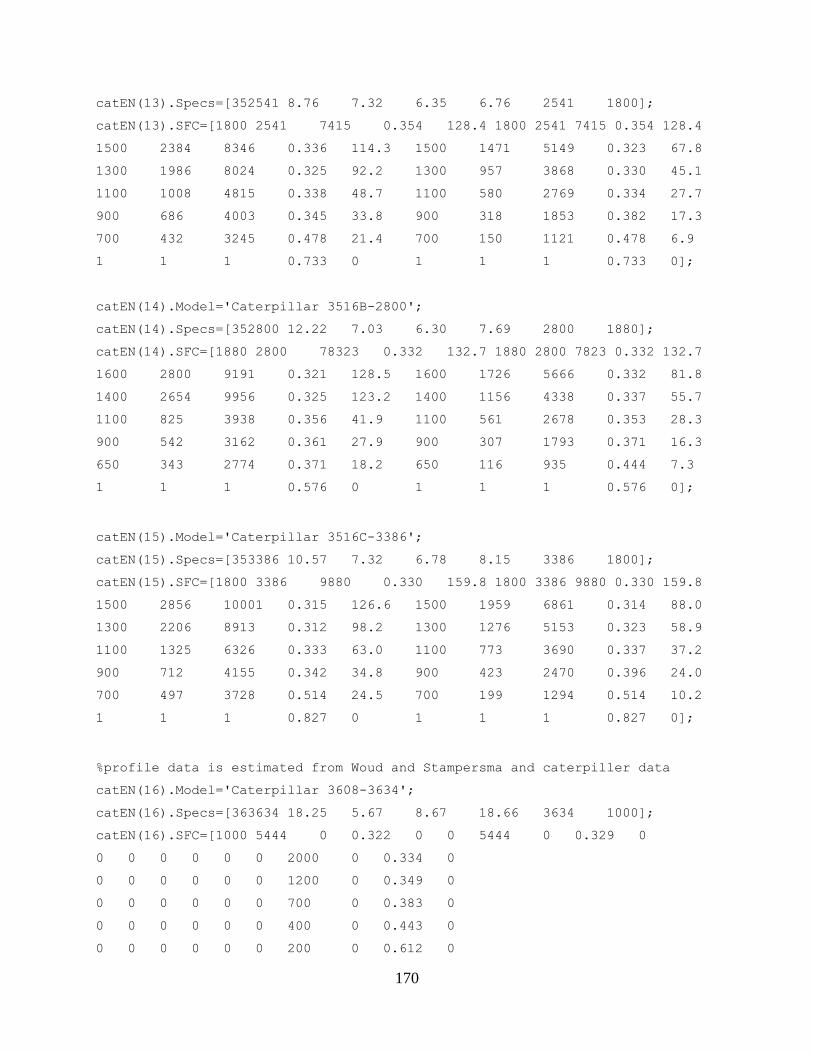
170
catEN(13).Specs=[352541 8.76 7.32 6.35 6.76 2541 1800];
catEN(13).SFC=[1800 2541 7415 0.354 128.4 1800 2541 7415 0.354 128.4
1500 2384 8346 0.336 114.3 1500 1471 5149 0.323 67.8
1300 1986 8024 0.325 92.2 1300 957 3868 0.330 45.1
1100 1008 4815 0.338 48.7 1100 580 2769 0.334 27.7
900 686 4003 0.345 33.8 900 318 1853 0.382 17.3
700 432 3245 0.478 21.4 700 150 1121 0.478 6.9
1 1 1 0.733 0 1 1 1 0.733 0];
catEN(14).Model='Caterpillar 3516B-2800';
catEN(14).Specs=[352800 12.22 7.03 6.30 7.69 2800 1880];
catEN(14).SFC=[1880 2800 78323 0.332 132.7 1880 2800 7823 0.332 132.7
1600 2800 9191 0.321 128.5 1600 1726 5666 0.332 81.8
1400 2654 9956 0.325 123.2 1400 1156 4338 0.337 55.7
1100 825 3938 0.356 41.9 1100 561 2678 0.353 28.3
900 542 3162 0.361 27.9 900 307 1793 0.371 16.3
650 343 2774 0.371 18.2 650 116 935 0.444 7.3
1 1 1 0.576 0 1 1 1 0.576 0];
catEN(15).Model='Caterpillar 3516C-3386';
catEN(15).Specs=[353386 10.57 7.32 6.78 8.15 3386 1800];
catEN(15).SFC=[1800 3386 9880 0.330 159.8 1800 3386 9880 0.330 159.8
1500 2856 10001 0.315 126.6 1500 1959 6861 0.314 88.0
1300 2206 8913 0.312 98.2 1300 1276 5153 0.323 58.9
1100 1325 6326 0.333 63.0 1100 773 3690 0.337 37.2
900 712 4155 0.342 34.8 900 423 2470 0.396 24.0
700 497 3728 0.514 24.5 700 199 1294 0.514 10.2
1 1 1 0.827 0 1 1 1 0.827 0];
%profile data is estimated from Woud and Stampersma and caterpiller data
catEN(16).Model='Caterpillar 3608-3634';
catEN(16).Specs=[363634 18.25 5.67 8.67 18.66 3634 1000];
catEN(16).SFC=[1000 5444 0 0.322 0 0 5444 0 0.329 0
0 0 0 0 0 0 2000 0 0.334 0
0 0 0 0 0 0 1200 0 0.349 0
0 0 0 0 0 0 700 0 0.383 0
0 0 0 0 0 0 400 0 0.443 0
0 0 0 0 0 0 200 0 0.612 0

171
0 0 0 0 0 0 1 0 0.863 0];
catEN(17).Model='Caterpillar 3612-5444';
catEN(17).Specs=[365444 15.92 5.75 11.67 25.57 5444 1000];
catEN(17).SFC=[1000 5444 0 0.322 0 0 5444 0 0.329 0
0 0 0 0 0 0 3158 0 0.333 0
0 0 0 0 0 0 1797 0 0.349 0
0 0 0 0 0 0 980 0 0.389 0
0 0 0 0 0 0 653 0 0.434 0
0 0 0 0 0 0 436 0 0.524 0
0 0 0 0 0 0 1 0 0.883 0];
catEN(18).Model='Caterpillar 3616-7268';
catEN(18).Specs=[367268 18 5.58 10.4 28.05 7268 1000];
catEN(18).SFC=[1000 7268 0 0.322 0 0 7268 0 0.329 0
0 0 0 0 0 0 4215 0 0.333 0
0 0 0 0 0 0 2398 0 0.349 0
0 0 0 0 0 0 1308 0 0.389 0
0 0 0 0 0 0 872 0 0.434 0
0 0 0 0 0 0 581 0 0.524 0
0 0 0 0 0 0 1 0 0.883 0];


