Integration Methods for MultidimensionalProbability Integrals

Abebe Geletu

abebe.geletu@tu-ilmenau.dewww.tu-ilmenau.de/simulation

Group of Simulation and Optimal Processes (SOP)Institute for Automation and Systems Engineering

Technische Universität Ilmenau

IFAC2011 Pre-Conference Tutorial

August 27-28, 2011, Milano

Content

1.Introduction

2.One-dimensional probability integrals

3.Cubature rules for multidimensional

3.1. Full-grid cubature rules

3.2. Sparse-grid cubature rules

4.Application

5.Conclusions

6.Resources and References

1. Introduction

u

min max

(CCOPT) min E[f (u, )]

Pr{g(u, ) 0}

u u .

s.t.

u

Task: to solve the optimization problem

Define:

g(u, ) 0

( ,0] ( ,0]

F(u) : E[f (u, )] f (u, ) ( )d

G(u) : Pr{g(u, ) 0} ( )d

1 (g(u, )) ( )d E[1 (g(u, ))]. = =

The problem CCOPT is equivalently written as

Introduction …

u

min max

(NLP) min F(u)

G(u) 0

u u u .

s.t.

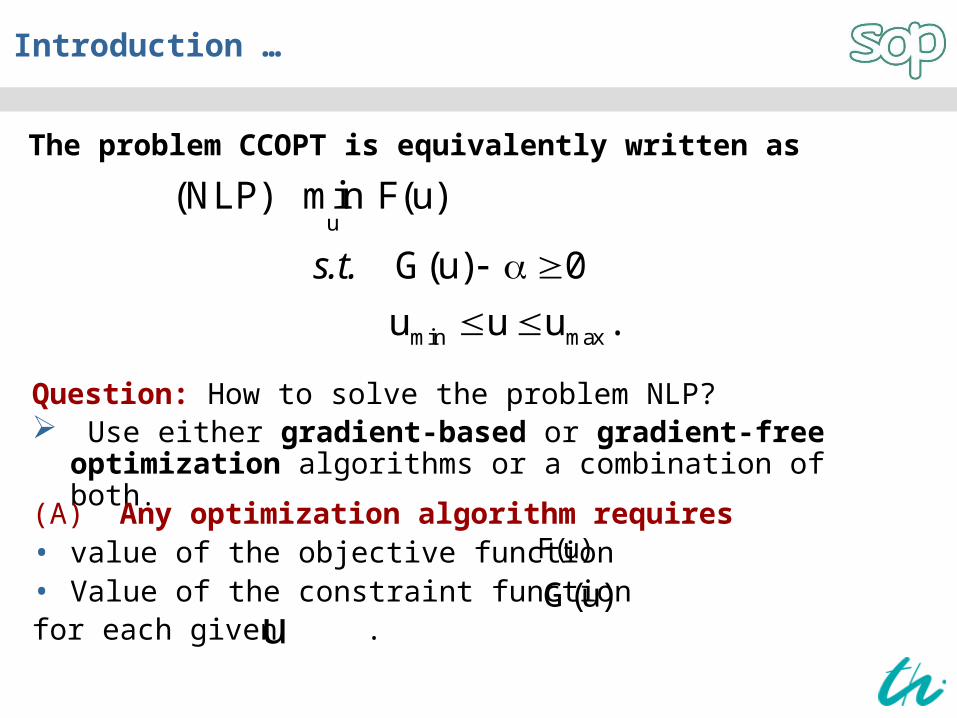
Question: How to solve the problem NLP? Use either gradient-based or gradient-free

optimization algorithms or a combination of both.

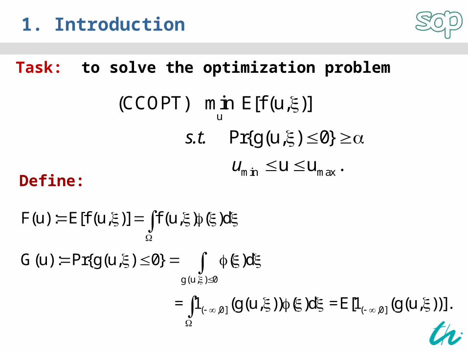
(A) Any optimization algorithm requires• value of the objective function • Value of the constraint function for each given .

F(u)

G(u)u

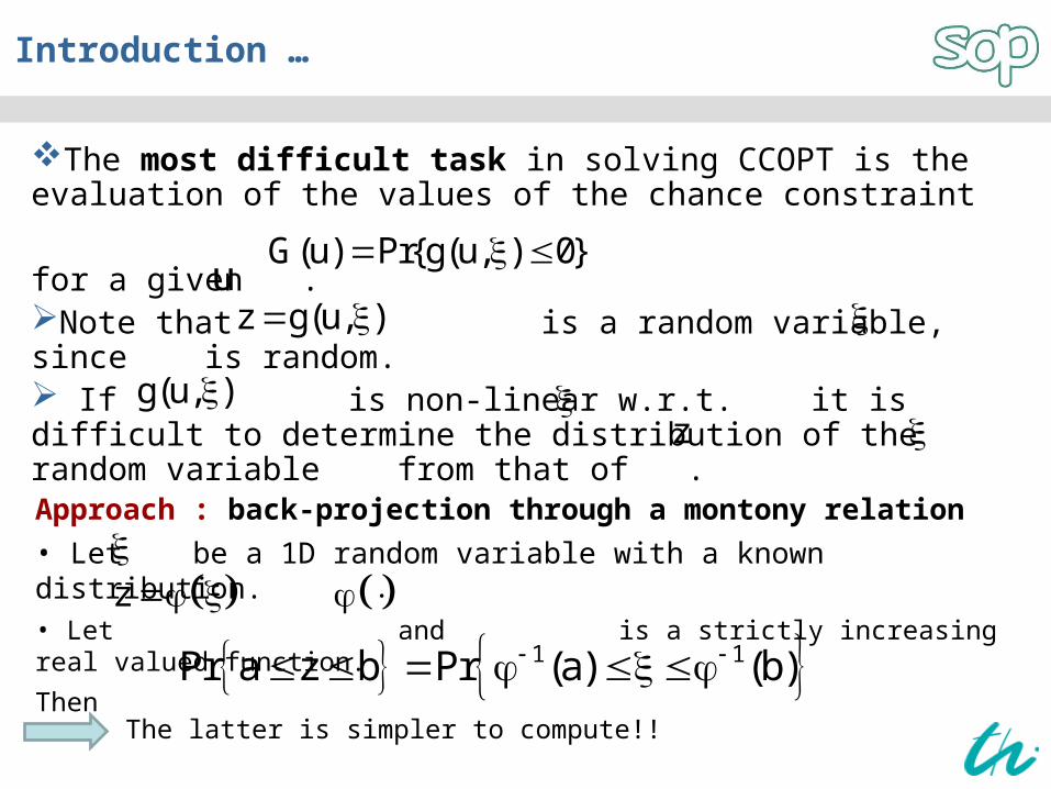
The most difficult task in solving CCOPT is the evaluation of the values of the chance constraint

for a given .Note that is a random variable, since is random. If is non-linear w.r.t. it is difficult to determine the distribution of the random variable from that of .

Introduction …

G(u) Pr{g(u, ) 0} u

z g(u, )

g(u, ) z

Approach : back-projection through a montony relation• Let be a 1D random variable with a known distribution. • Let and is a strictly increasing real valued function.

Then

z

1 1Pr a z b Pr (a) (b) The latter is simpler to compute!!

Introduction …

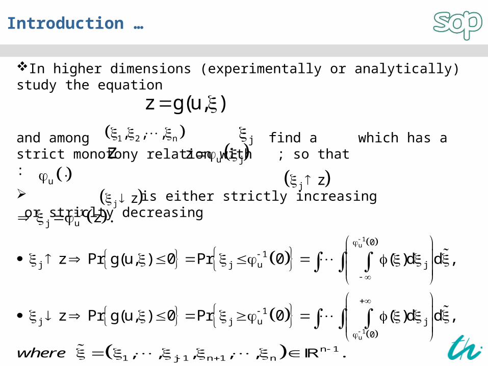
In higher dimensions (experimentally or analytically) study the equation

and among find a which has a strict monotony relation with ; so that :

is either strictly increasing or striclty decreasing

z g(u, )

1u

1u

1j u

0

1j j u j

1j j u j

0

z .

z Pr g(u, ) 0 Pr 0 ( )d d ,

z Pr g(u, ) 0 Pr 0 ( )d d ,

1 2 n, , , jz u jz

u j z j z

n 11 j 1 n 1 n, , , , , .where

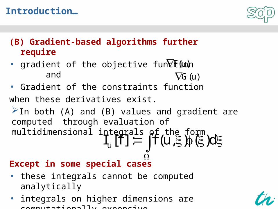
(B) Gradient-based algorithms further require

• gradient of the objective function and• Gradient of the constraints function when these derivatives exist.

Introduction…

F(u)G(u)

In both (A) and (B) values and gradient are computed through evaluation of multidimensional integrals of the form

uI [f ] : f (u, ) ( )d

Except in some special cases• these integrals cannot be computed analytically• integrals on higher dimensions are computationally

expensive

Introduction…

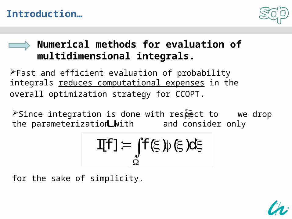
Numerical methods for evaluation of multidimensional integrals.

Fast and efficient evaluation of probability integrals reduces computational expenses in the overall optimization strategy for CCOPT.

I[f ] : f (x) (x)dx

Since integration is done with respect to we drop the parameterization with and consider only

for the sake of simplicity.

u

I[f ] : f ( ) ( )d

Methods for Multidimensional Integrals Deterministic Methods

• Quadrature rules – for 1D integrals

• Full or Spars-grid cubature rules – for MD integrals

Sampling-based Methods

• Monte Carlo Methods

• Quasi-Monte Carlo methods

Deterministic integration rules for multidimensional integrals (commonly called cubature rules) are usually constructed from 1D quadrature rules.

Introduction …

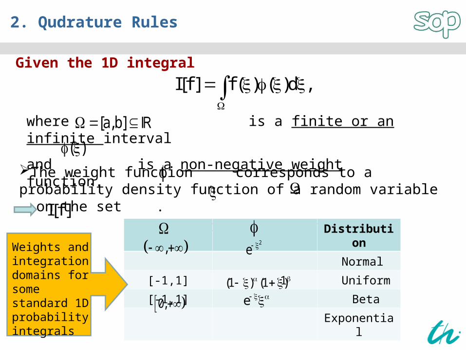
2. Qudrature Rules

I[f ] f ( ) ( )d ,

where is a finite or an infinite interval

and is a non-negative weight function.

The weight function corresponds to a probability density function of a random variable on the set . represents expected value.

Given the 1D integral

[a, b] ( )

I[f ] Distributio

n

Normal

[-1,1] 1 Uniform

[-1,1] Beta

Exponential

, 2

e

(1 ) (1 ) e 0,

Weights and integration domains for some standard 1D probability integrals

Qudrature Rules …

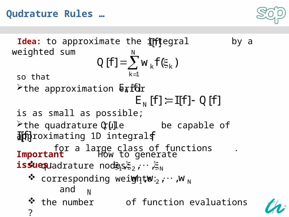
Idea: to approximate the integral by a weighted sum

so that the approximation error

is as small as possible;the quadrature rule be capable of approximating 1D integrals for a large class of functions .

N

k kk 1

Q[f ] w f ( )

I[f ]

NE [f ] : I[f ] Q[f ] NE [f ]

Q[ ]fI[f ]

quadrature nodes: corresponding weights: and the number of function evaluations ?

Important issues: 1 2 N, , ,

1 2 Nw , w , , wN

How to generate

Qudrature Rules …

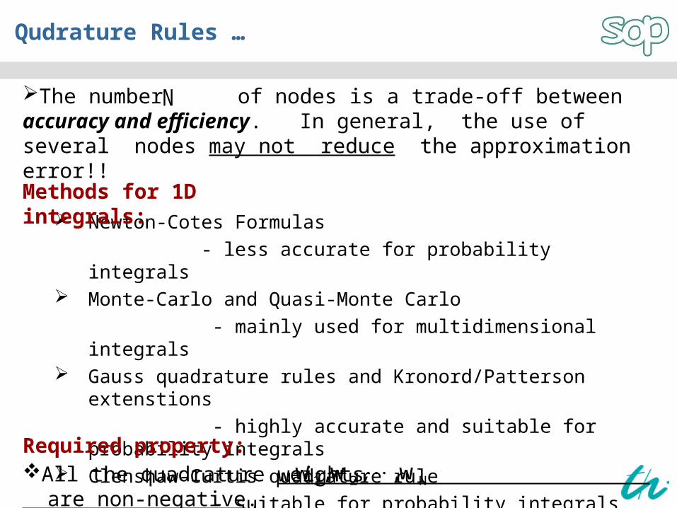
Newton-Cotes Formulas - less accurate for probability integrals Monte-Carlo and Quasi-Monte Carlo - mainly used for multidimensional integrals Gauss quadrature rules and Kronord/Patterson

extenstions - highly accurate and suitable for probability

integrals Clenshaw-Curtis quadrature rule - suitable for probability integrals

Methods for 1D integrals:

The number of nodes is a trade-off between accuracy and efficiency. In general, the use of several nodes may not reduce the approximation error!!

N

Required property: All the quadrature weights are non-negative.

1 2 Nw , w , , w

Quadrature Rules …

Non-negative quadrature weights have advantages: the use of non-negative weights reduces the danger of numerical cancellations in ; in stochastic optimization, if is convex w.r.t. u for each fixed , then

is convex and due to the non-negative of weights the approximation

preserves the convexity.

(u) f (u, ) ( )d

Q[ ]

N

k kk 1

(u) w f (u, )

(u) : f ,

Orthogonal Polynomials and Gauss Quadrature Rules

Quadrature nodes and corresponding weights are computed based on orthogonal polynomials with respect to a given pair .

1 2 N, , , 1 2 Nw , w , , w

• For two functions and

defines a scalar product w.r.t. on the set . • A degree n polynomial and a degree m polynomial are orthogonal on w.r.t. if

• Different pairs lead to different sets of orthogonal polynomials.

,

Ref: Walter Gatushi : Orthogonal Polynomials

f g f ,g f g d

np mp

n m n mp ,p p p d 0.

Example: Sets of orthogonal polynomials for standard pair:• Hermit polynomials -• Jacobi polynomials - etc.

, 2

( ) e , , . ( ) (1 ) (1 ) , , 1; 1,1 ;

,

Generation of orthogonal polynomials

Given any pair . Let and all moments

exist and finite. Then

(i)there is a unique set of orthogonal polynomials

corresponding to satisfying

(ii) the set of polynomials are uniquely determined by the three-term recurrence relation using and

where and

0k

k ( )d ,k 0,1,

k mp ,p 0, k m for

k 1 k 1 k k k 1p ( ) a p ( ) b p ( ), k 1,2,

1p ( ) : 0

k 1k k k 1 k 1

1, k 0b

p ,p p ,p , k 1,2,

for

for

k 1 k k k ka p ,p p ,p , k 0, 1, 2,

Ref: Walter Gatushi : Orthogonal Polynomials

, 0 1 2p 1,p ( ), p ( ),

0p ( ) 1

,

Computation of Gauss quadrature nodes and weights

1 2 N, , ,

Ref: Golub, G.H., Welsch, J.H. Calculation of Gauss quadrature rules.

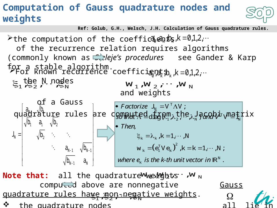
the computation of the coefficients of the recurrence relation requires algorithms (commonly known as Steleje’s procedures see Gander & Karp for a stable algorithm.

0 k ka ,a , b ,k 0,1,2,

For known recurrence coefficients the N nodes

and weights of a Gauss

quadrature rules are computed from the Jacobi matrix

0 k ka ,a , b ,k 0,1,2,

0 1

1 1 2

N 2

N 1 N 1

N 1 N

a b

b a b

J b

a b

b a

1 2 Nw , w , , w

TN

T1 2 N N

k k

2Tk 1 k

Nk

J V V;

diag( , , , ) V I

,k 1, , N

w e Ve ,k k 1, , N;

.

Factorize

so that and V

Then,

where e is the k-th unit vector in

Note that: all the quadrature weights computed above are nonnegative Gauss quadrature rules have non-negative weights. the quadrature nodes all lie in the interior of .

1 2 Nw , w , , w

1 2 N, , ,

Standard Gauss Quadrature Rules

Orthogona

l Polynomia

ls

Quadrature Rule

1 Lgendre Gauss-Legendre

Chebychev Gauss-Chebychev

Jacobi Gauss-Jacobi

Laguerr Gauss-Laguerr

Hermite Gauss-Hermite

[ 1,1]

[ 1,1] 21

1

[ 1,1] (1 ) (1 ) ; , 1

[0, ) e

( , ) 2

e

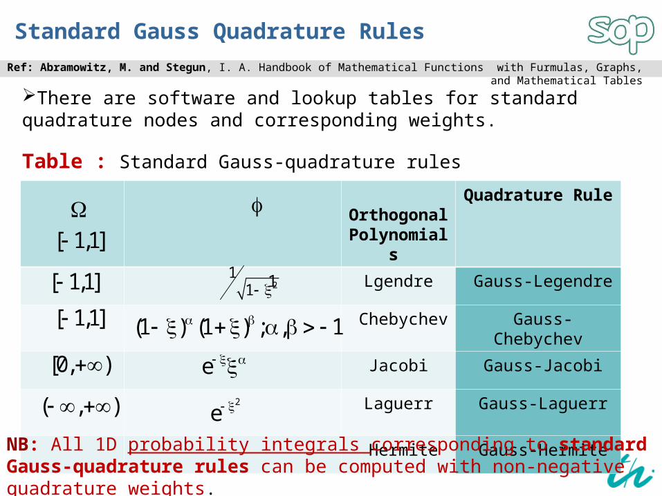
There are software and lookup tables for standard quadrature nodes and corresponding weights.

Ref: Abramowitz, M. and Stegun, I. A. Handbook of Mathematical Functions with Furmulas, Graphs, and Mathematical Tables

Table : Standard Gauss-quadrature rules

NB: All 1D probability integrals corresponding to standard Gauss-quadrature rules can be computed with non-negative quadrature weights.

Gauss Quadrature Rules – Exactness

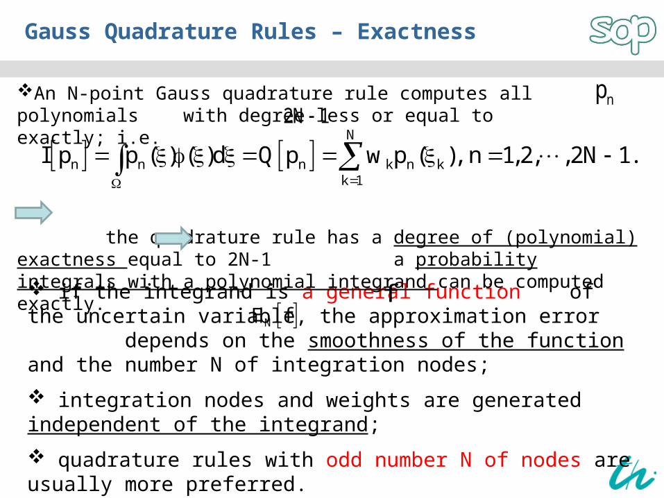
if the integrand is a general function of the uncertain variable, the approximation error depends on the smoothness of the function and the number N of integration nodes;

integration nodes and weights are generated independent of the integrand;

quadrature rules with odd number N of nodes are usually more preferred.

f NE f

An N-point Gauss quadrature rule computes all polynomials with degree less or equal to exactly; i.e.

the quadrature rule has a degree of (polynomial) exactness equal to 2N-1 a probability integrals with a polynomial integrand can be computed exactly.

np2N 1

N

n n n k n kk 1

I p p ( ) ( )d Q p w p ( ), n 1,2, , 2N 1.

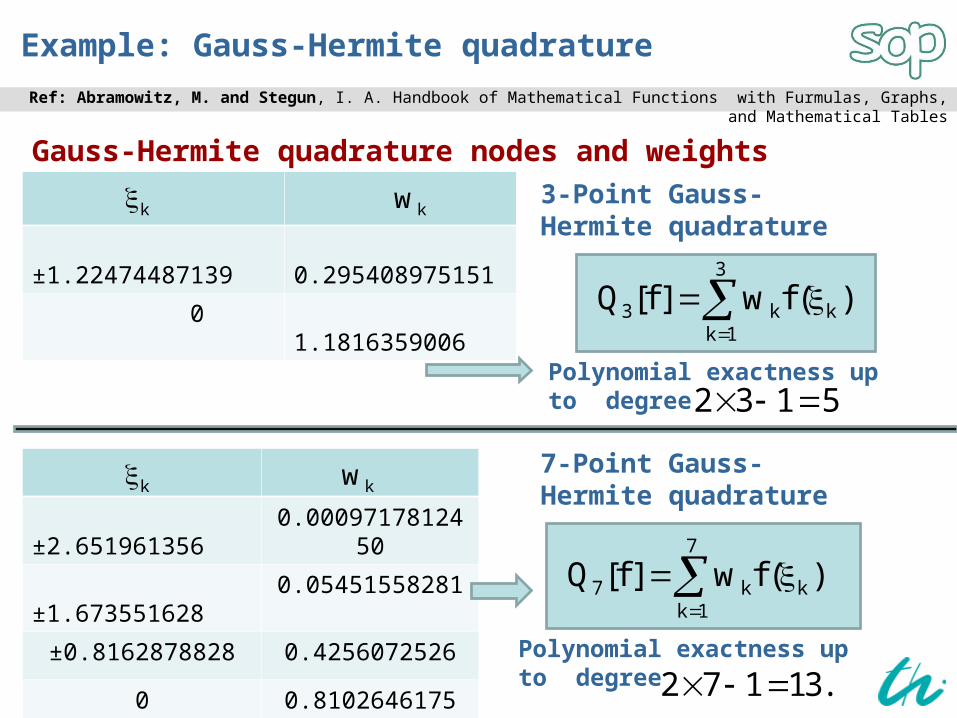
Example: Gauss-Hermite quadrature

Gauss-Hermite quadrature nodes and weights

±1.22474487139 0.295408975151

0 1.1816359006

k kw

±2.651961356 0.0009717812450

±1.673551628 0.05451558281

±0.8162878828 0.4256072526

0 0.8102646175

k kw

Ref: Abramowitz, M. and Stegun, I. A. Handbook of Mathematical Functions with Furmulas, Graphs, and Mathematical Tables

3-Point Gauss-Hermite quadrature

3

3 k kk 1

Q [f ] w f ( )

2 3 1 5 Polynomial exactness up to degree

7-Point Gauss-Hermite quadrature

7

7 k kk 1

Q [f ] w f ( )

Polynomial exactness up to degree2 7 1 13.

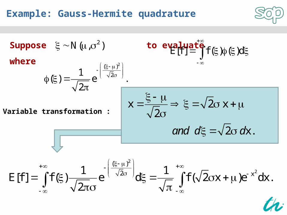
Example: Gauss-Hermite quadrature

Suppose to evaluate

whereE[f ] f ( ) ( )d

2N( , )

2( )

21( ) e .

2

Variable transformation :x 2 x

2

2 x.

and d d

2

2

( )

2 x1 1E[f ] f ( ) e d f ( 2 x )e dx.

2

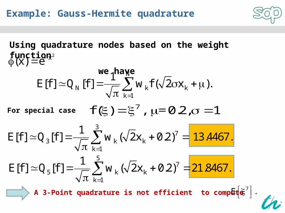
Example: Gauss-Hermite quadrature

Using quadrature nodes based on the weight function

we have

2x(x) e N

N k kk 1

1E[f ] Q [f ] w f ( 2 x ).

7f ( ) , 0.2, 1 = For special case

37

3 k kk 1

1E[f ] Q [f ] w ( 2x 0.2) 13.4467.

57

5 k kk 1

1E[f ] Q [f ] w ( 2x 0.2) 21.8467.

A 3-Point quadrature is not efficient to compute 7E .

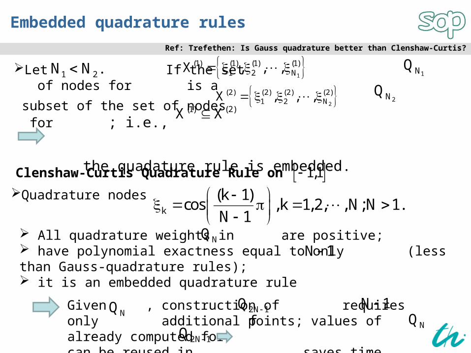
Embedded quadrature rules

Ref: Trefethen: Is Gauss quadrature better than Clenshaw-Curtis?

Let If the set of nodes for is a

subset of the set of nodes for ; i.e.,

the quadature rule is embedded.

1NQ 1

(1) (1) (1) (1)1 2 NX , , ,

2

(2) (2) (2) (2)1 2 NX , , , 2NQ

1 2N N .

(1) (2)X X

Clenshaw-Curtis Quadrature Rule on

Quadrature nodes k

(k 1)cos ,k 1,2, , N; N 1.

N 1

All quadrature weights in are positive; have polynomial exactness equal to only (less than Gauss-quadrature rules); it is an embedded quadrature rule

N 1NQ

Given , construction of requires only additional points; values of already computed forcan be reused in saves time.

NQ 2N 1Q N 1f NQ

2N 1Q

1,1

Advantages of Embedded quadrature rules

nodes of lower degree quadrature can be used when constructing higher degree quadratures; provides easier error estimation for quadrature rule; embeddedness is a highly desired property for the construction of multidimensional cubature techniques, etc.

Unfortunately, Gauss quadratture rules are not embedded.

Example: Gauss-Hermite quadrature

N Nodes

1 0

2 -1,1

3

4

5

3,0, 3

3 5 , 3 6 , 3 5 , 3 6

5 15 , 5 15 ,0, 5 15 , 5 15

Some advantages of embedded rules:

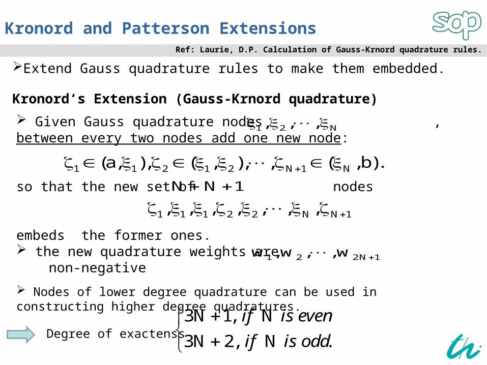
Kronord and Patterson Extensions

Nodes of lower degree quadrature can be used in constructing higher degree quadratures.

Extend Gauss quadrature rules to make them embedded.

Given Gauss quadrature nodes , between every two nodes add one new node:

so that the new set of nodes

embeds the former ones. the new quadrature weights are non-negative

Kronord‘s Extension (Gauss-Krnord quadrature)

1 1 2 1 2 N 1 N(a, ), ( , ), , ( , b).

1 2 N, , ,

1 1 1 2 2 N N 1, , , , , , , N N 1

1 2 2N 1w , w , , w

Degree of exactenss3N 1, N

3N 2, N

if is even

if is odd.

Ref: Laurie, D.P. Calculation of Gauss-Krnord quadrature rules.

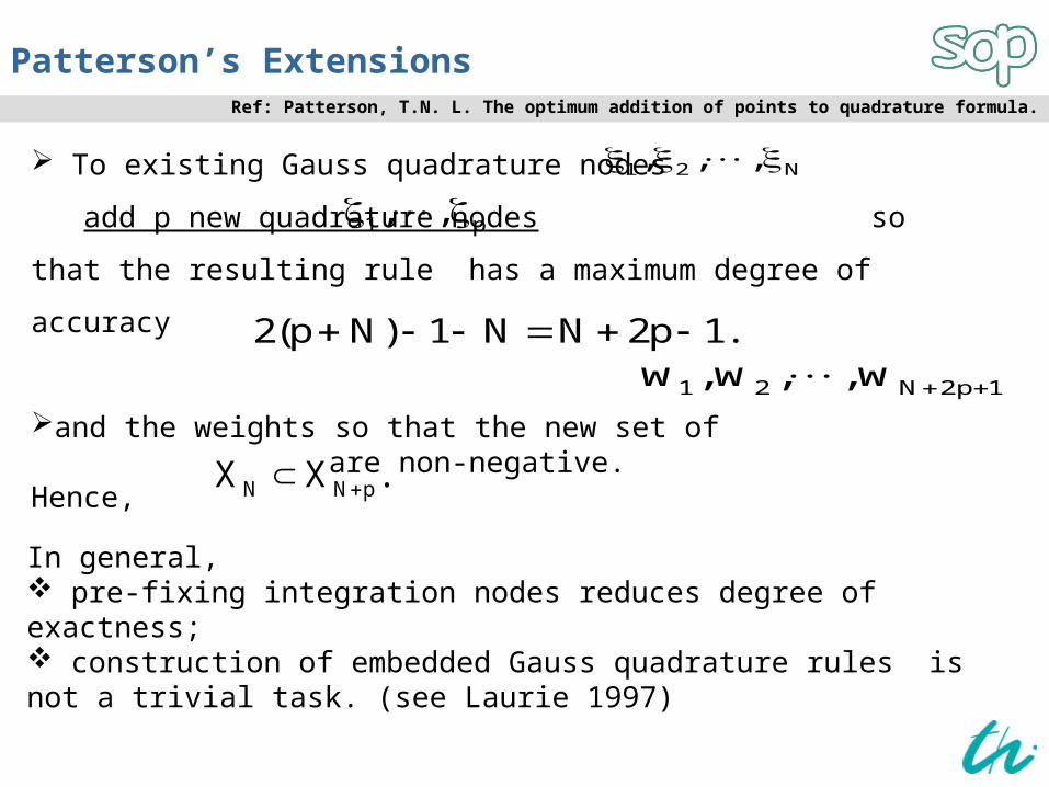
Patterson’s Extensions

To existing Gauss quadrature nodes add p new

quadrature nodes so that the resulting rule has a

maximum degree of accuracy

and the weights so that the new set of are non-negative.Hence,

2(p N) 1 N N 2p 1.

1 2 N, , ,

1 p, ,

1 2 N 2p 1w , w , , w

N N pX X .

In general, pre-fixing integration nodes reduces degree of exactness; construction of embedded Gauss quadrature rules is not a trivial task. (see Laurie 1997)

Ref: Patterson, T.N. L. The optimum addition of points to quadrature formula.

Quadrature for non-standard integrals

transform integrals on non-standard intervals onto the standard ones.

Note that:

a 1

1

1f ( ) ( )d f ( ) ( )d , a

1 using ;

Examples of some possible transformations:

etc.

b 1

a 1

b af ( ) ( )d f ( ) ( )d , 1 ( a);

2 using

1

a 1

1f ( ) ( )d f ( ) ( )d , a

1 using ;

• transformation is done in such a way the resulting integral is easier to compute;• when possible to try to match the resulting weight function and integration domain, so that available results can be easily used.

Quadrature for non-standard integrals

a 1

21

1a

1

1 1 1f ( )d f a d .

2 1 (1 )

Usinging we obtain

-

Example

The transformed integral can be computed using either Gauss-Legendre or Gauss-Chebychev quadrature rule.

h(u) 1

21

1 1 1p(u) Pr h(u) 0 ( )d p(u) h(u) d .

2 1 (1 ) -

This can be applied to a chance constraint as

From Chance to Expected Value Constraint

Example:

i i

0 0 2A B A B B A B i A Bx (C ,C , r , r ,R ,T), u (Q,V,F), (C ,C ,T ,k ,k ) N( , ). and

with

Ref: Geletu et al: Monotony Analysis and Sparse-Grid Integration for nonlinear Chance Constrained Process Optimization

Monotony relationiA BC R

mini iAi

min minB B A A C u,x,

Pr R R Pr C C ( )d ,

using the change of variables

where

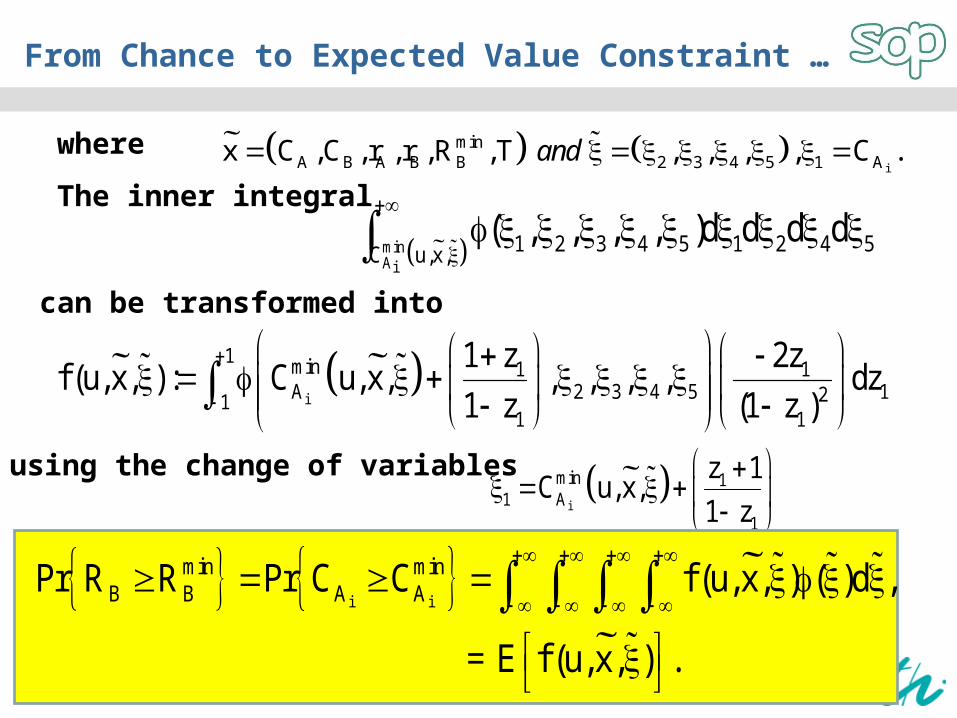
From Chance to Expected Value Constraint …

i

minA B A B B 2 3 4 5 1 Ax C ,C , r , r ,R ,T , , , , C . and

minAi

1 2 3 4 5 1 2 4 5C u,x,( , , , , )d d d d

The inner integral

can be transformed into

i

1 min 1 1A 2 3 4 5 121

1 1

1 z 2zf (u, x, ) : C u, x, , , , , dz

1 z (1 z )

i

min 11 A

1

z 1C u, x,

1 z

i i

min minB B A APr R R Pr C C f (u, x, ) ( )d ,

E f (u, x, ) . =

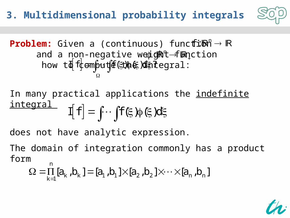
3. Multidimensional probability integrals

Problem: Given a (continuous) function and a non-negative weight function how to compute the integral: I f f ( ) ( )d ?

In many practical applications the indefinite integral

nf : n:

I f f ( ) ( )d does not have analytic expression.

The domain of integration commonly has a product form

n

k k 1 1 2 2 n nk 1

[a , b ] [a , b ] [a , b ] [a , b ]

Standard integration domains

n

n n n

[ 1,1]

( , ) , [0,1] , [0, )

- unform dis

Note: Transform non-standard integrals into standard forms.Example: Let be a random variable w.r.t. the probability measure

such that and Then

represents the expected value of w.r.t. the probability measure .

Integration domain

Related probabilbility distribution

Uniform

Normal

Beta, Drichlet

Exponential, Gamma, Lognormal, Weibull

n[ 1,1] n( , )

n[0,1]n[0, )

d ( ) ( )d n | ( ) 0 .

I f f ( ) ( )d

f E f

Multidimensional probability integrals …

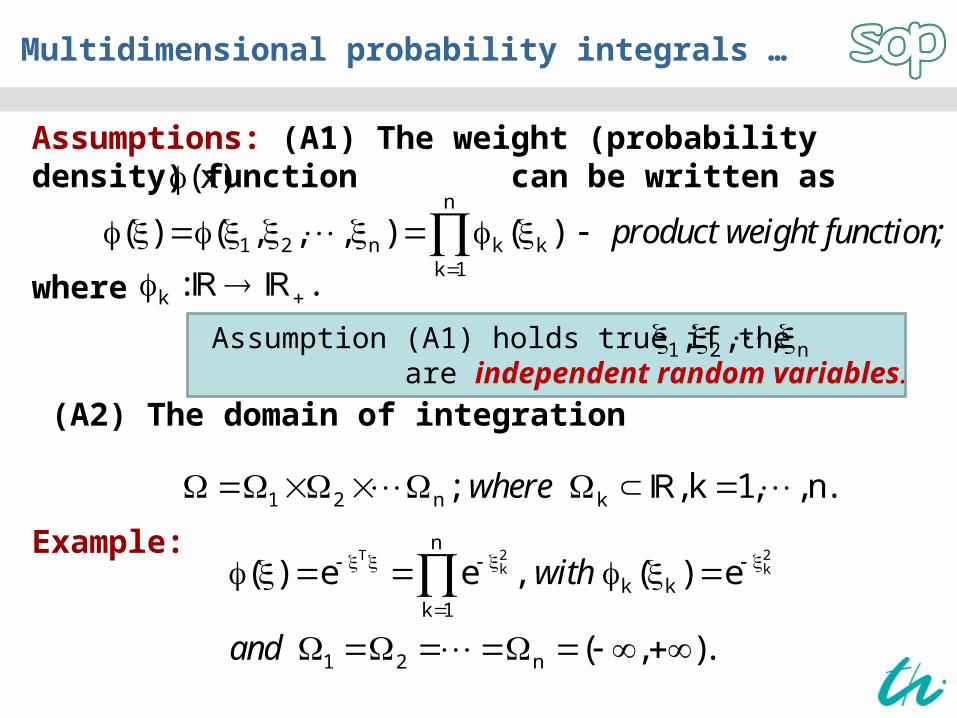
Assumption (A1) holds true if the are independent random variables.

Assumptions: (A1) The weight (probability density) function can be written as (x)

n

1 2 n k kk 1

( ) ( , , , ) ( ) product weight function;

where k : .

1 2 n, , ,

(A2) The domain of integration

1 2 n k; , k 1, , n. where

Example: 2 2Tk k

n

k kk 1

1 2 n

( ) e e , ( ) e

( , ).

with

and

Multidimensional probability integrals …

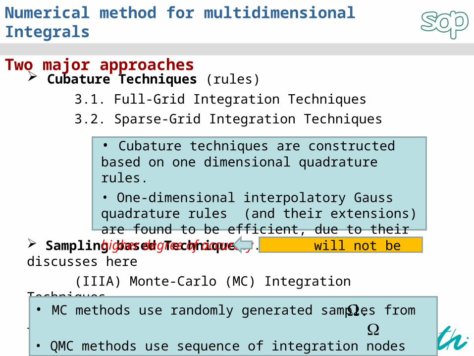
Numerical method for multidimensional Integrals

Two major approaches Cubature Techniques (rules)

3.1. Full-Grid Integration Techniques

3.2. Sparse-Grid Integration Techniques

Sampling based Techniques will not be discusses here

(IIIA) Monte-Carlo (MC) Integration Techniques

(IIIB) Quasi-Monte-Carlo (QMC) Integration Techniques

• Cubature techniques are constructed based on one dimensional quadrature rules.• One-dimensional interpolatory Gauss quadrature rules (and their extensions) are found to be efficient, due to their higher degree of accuracy.

• MC methods use randomly generated samples from

• QMC methods use sequence of integration nodes from with lower discrepancy.

.

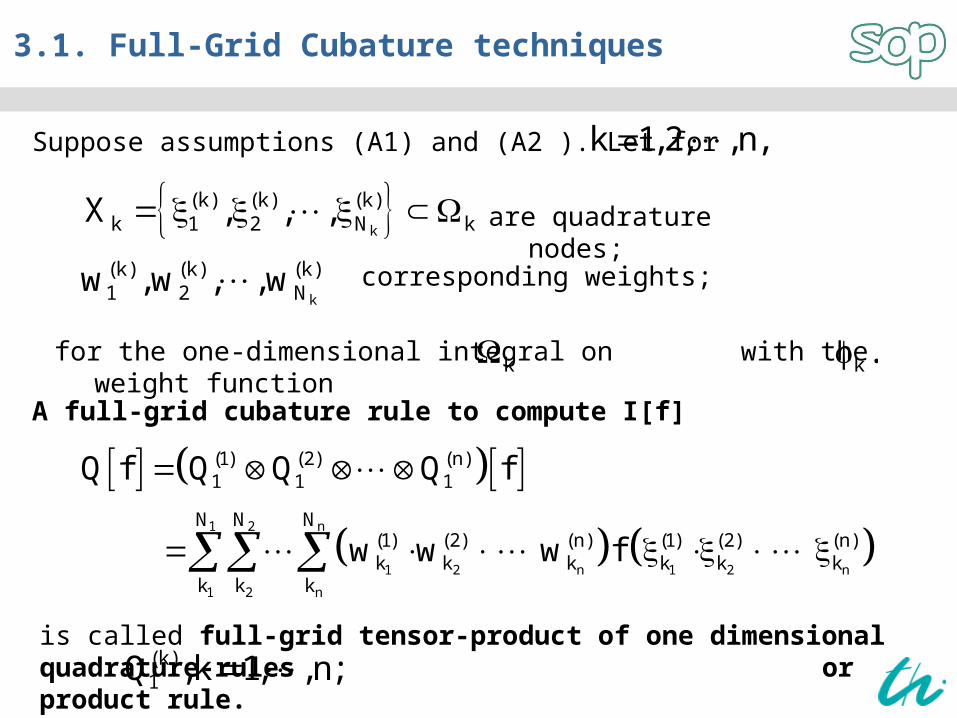
3.1. Full-Grid Cubature techniques

Suppose assumptions (A1) and (A2 ). Let for k 1,2, , n,

k

(k) (k) (k)k 1 2 N kX , , , are quadrature nodes;

k

(k) (k) (k)1 2 Nw , w , , w corresponding weights;

for the one-dimensional integral on with the weight function

k k .

A full-grid cubature rule to compute I[f]

1 2 n

1 2 n 1 2 n

1 2 n

(1) (2) (n)1 1 1

N N N(1) (2) (n) (1) (2) (n)k k k k k k

k k k

Q f Q Q Q f

w w w f

(k)1Q ,k 1, , n;

is called full-grid tensor-product of one dimensional quadrature-rules or product rule.

How good are full-grid cubature techniques?

Important questions: How many grid-points are there in the full-grid cubature rule

? That is, the set

Is it necessary to use all the grid points in ? Is there redundancy in the full-grid scheme?

What is the polynomial (or degree) of exactness of ?

1 2 n i

1 2 n

(1) (2) (n) (i)k k k k i i i

X X X X

, , , X ,k 1, , N ,i 1, , n

The number of grid-points (integration nodes) in :

1 2 n#X N N N .

n#X N

If then the number of grid points will be

Q f

X

Q f

Q f

1 2 nN N N : N,

exponential growth!!

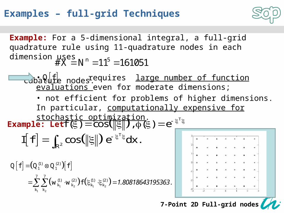
Examples – full-grid Techniques

Example: For a 5-dimensional integral, a full-grid quadrature rule using 11-quadrature nodes in each dimension uses

cubature nodes.n 5#X N 11 161051 • requires large number of function evaluations even for moderate dimensions;• not efficient for problems of higher dimensions. In particular, computationally expensive for stochastic optimization.

Q f

Example: Let T

f ( ) cos , ( ) e

T

2I f cos e dx.

1 2 1 2

1 2

(1) (2)1 1

7 7(1) (2) (1) (2)k k k k

k k

Q f Q Q f

w w f . 1.80818643195363

7-Point 2D Full-grid nodes

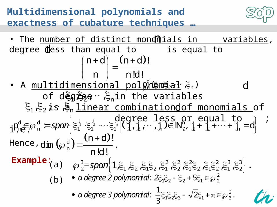
Multidimensional polynomials and exactness of cubature techniques

One measure of quality for a cubature rule is related with the largest degree polynomial that it can integrate exactly.

For the variables a monomial of degree in the variables is an expression of the form

where

1 2 n, , , d n

j j j1 2 n

1 1 1

n1 2 n 0 1 2 nj , j , , j j j j d. and

Example: For two variables

(a)the following are monomials of degree 3

(b) all monomials in the two

variable of degree less equal to 3 are

1 2 and

3 0 3 2 1 3 0 2 0 3 31 2 1 1 2 1 2 1 2 1 2 2,= , , , =

1 2

2 21 2 1 2

3 2 2 31 1 2 1 2 2

0 1

1 ,

2 , ,

3 , , ,

degree monomial

(a)

(b)

• A multidimensional polynomial of degree in the variables is a linear combination of monomials of degree less or equal to ; i.e.

Multidimensional polynomials and exactness of cubature techniques …

• The number of distinct monomials in variables, degree less than equal to is equal to

nd

n d n d !

n n!d!

dn 1 2 np ( , , , ) d

1 2 n, , , 1 2 n, , , d

j j j1 2 nd d n

n n 1 1 1 1 2 n 0 1 2 np : j , j , , j j j j dspan ,

Hence, dn

n d !dim .

n!d!

Example: 3 2 2 2 2 3 32 1 2 1 2 1 2 1 2 1 2 1 21, , , , , , , , , .=span

21 2 2 1 2

31 2 3 1 3

5

12 .

3

a degree 2 polynomial: 2

a degree 3 polynomial:

A cubature rule is said to be exact for a polynomial if

That is,

Multidimensional polynomials and exactness of cubature techniques …

Q f dnp

1 2 n

1 2 n

1 2 n 1 2 n

1 2 n

dn 1 n

N N N(1) (2) (n) d (1) (2) (n)k k k n k k k

k k k

p ( , , ) ( )

w w w p .

d dn nI p p .=Q

A cubature rule is said to have a polynomial exactness (or degree of accuracy) if it is exact for all polynomials of degree less than equal to .

Q fd

d

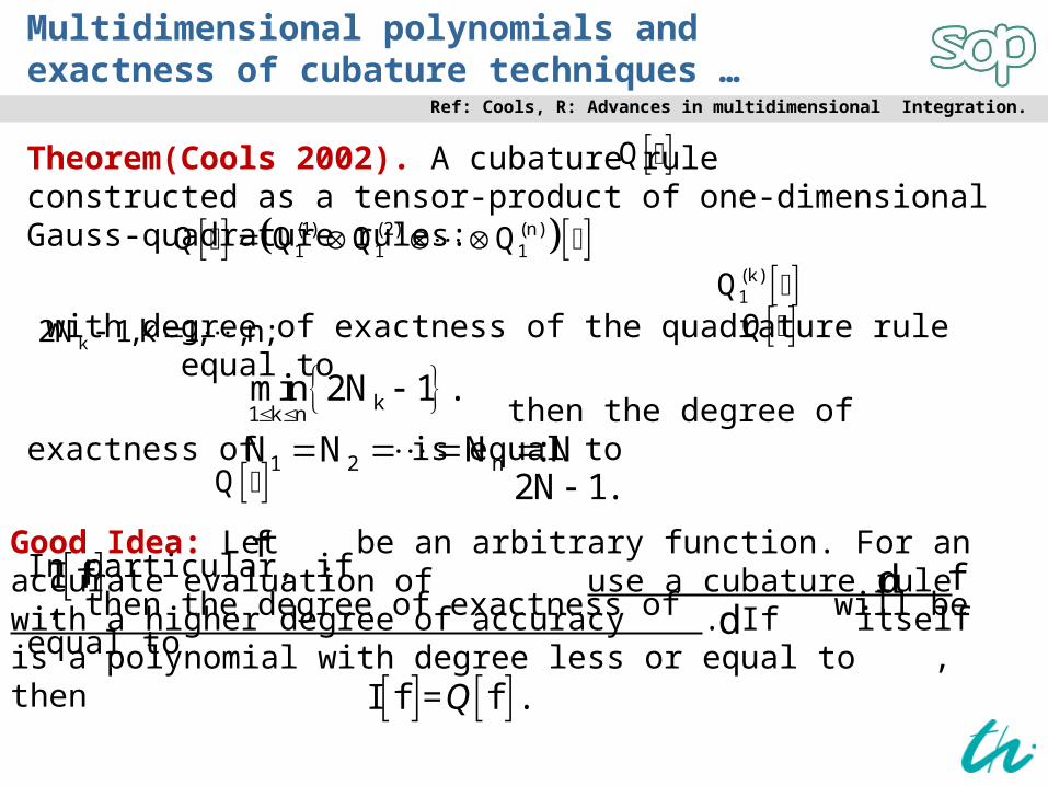
Ref: Cools, R: Advances in multidimensional Integration.

Theorem(Cools 2002). A cubature rule constructed as a tensor-product of one-dimensional Gauss-quadrature rules:

with degree of exactness of the quadrature rule equal to then the degree of exactness of is equal to

In particular, if , then the degree of exactness of will be equal to

Multidimensional polynomials and exactness of cubature techniques …

Good Idea: Let be an arbitrary function. For an accurate evaluation of use a cubature rule with a higher degree of accuracy . If itself is a polynomial with degree less or equal to , then

k1 k nmin 2N 1 .

Ref: Cools, R: Advances in multidimensional Integration.

(1) (2) (n)1 1 1Q Q Q Q

(k)1Q

k2N 1,k 1, , n; Q

Q

1 2 nN N N : N Q 2N 1.

f I f d f

d

I f f .=Q

Fact: Higher accuracy in computing can be achieved by using a cubature rule with higher degree of exactness.

I f

2 21 2

2

2 21 2 1 2I f cos e d d .

Example: Consider a full-grid 2D cubaturer for the integral

Number of 1D quadrature nodes

Cubature 2D nodes

7 1.80818643195363

17 1.80818642926362

27 49217 289

Q f

Almost equal result from two full-grids

Multidimensional polynomials and exactness of cubature techniques …

min max

2 Required Number of Nodes

n dn dN N

nn

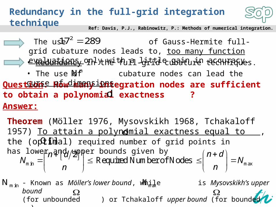
The use of Gauss-Hermite full-grid cubature nodes leads to, too many function evaluations only with a little gain in accuracy.

Redundancy in the full-grid integration technique

217 289

Question: How many integration nodes are sufficient to obtain a polynomial exactness ?

nN

d

• Redundancy in the full-grid cubature techniques. • The use of cubature nodes can lead the curse of dimensions.

Answer:

Theorem (Möller 1976, Mysovskikh 1968, Tchakaloff 1957) To attain a polynomial exactness equal to , the (optimal) required number of grid points in has lower and upper bounds given by

dQ[ ]

minN - Known as Möller’s lower bound, while is Mysovskikh’s upper bound(for unbounded ) or Tchakaloff upper bound (for bounded ).

maxN

Ref: Davis, P.J., Rabinowitz, P.: Methods of numerical integration.

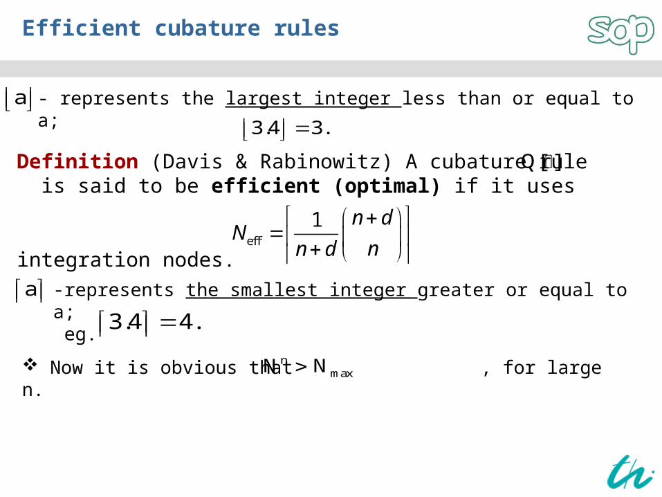
Definition (Davis & Rabinowitz) A cubature rule is said to be efficient (optimal) if it uses

integration nodes.

Now it is obvious that , for large n.

Efficient cubature rules

- represents the largest integer less than or equal to a; a 3.4 3.

Q[ ]

eff

1 n dN

nn d

a -represents the smallest integer greater or equal to a; eg. 3.4 4.

nmaxN N

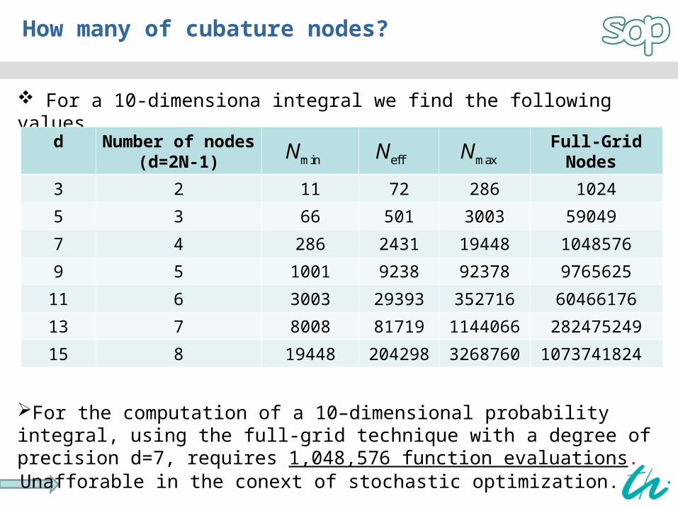
For a 10-dimensiona integral we find the following values

How many of cubature nodes?

d Number of nodes (d=2N-1)

Full-Grid Nodes

3 2 11 72 286 1024

5 3 66 501 3003 59049

7 4 286 2431 19448 1048576

9 5 1001 9238 92378 9765625

11 6 3003 29393 352716 60466176

13 7 8008 81719 1144066 282475249

15 8 19448 204298 3268760 1073741824

minN effN maxN

For the computation of a 10–dimensional probability integral, using the full-grid technique with a degree of precision d=7, requires 1,048,576 function evaluations.

Unafforable in the conext of stochastic optimization.

effN

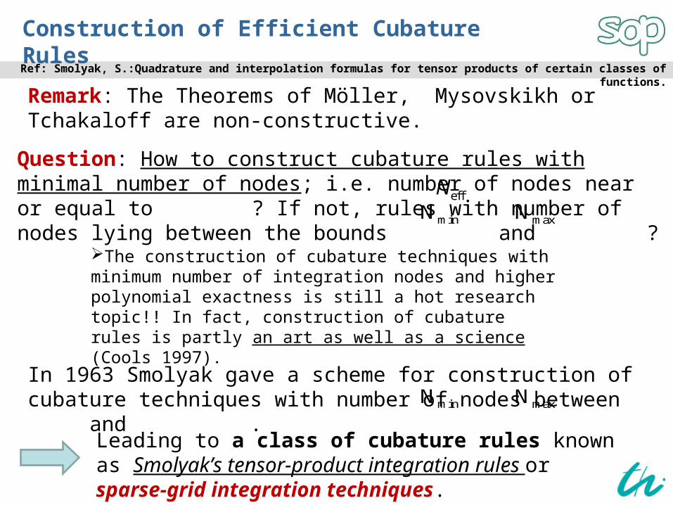
Remark: The Theorems of Möller, Mysovskikh or Tchakaloff are non-constructive.

Construction of Efficient Cubature Rules

Question: How to construct cubature rules with minimal number of nodes; i.e. number of nodes near or equal to ? If not, rules with number of nodes lying between the bounds and ?

maxNminN

Ref: Smolyak, S.:Quadrature and interpolation formulas for tensor products of certain classes of functions.

In 1963 Smolyak gave a scheme for construction of cubature techniques with number of nodes between and . minN maxN

Leading to a class of cubature rules known as Smolyak’s tensor-product integration rules or sparse-grid integration techniques.

The construction of cubature techniques with minimum number of integration nodes and higher polynomial exactness is still a hot research topic!! In fact, construction of cubature rules is partly an art as well as a science (Cools 1997).

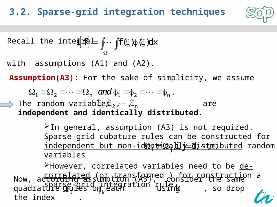
3.2. Sparse-grid integration techniques

Recall the integral

with assumptions (A1) and (A2).

I f f ( ) ( )dx

Assumption(A3): For the sake of simplicity, we assume

1 2 n 1 2 n . and The random variables are independent and identically distributed.

1 2 n, , ,

In general, assumption (A3) is not required. Sparse-grid cubature rules can be constructed for independent but non-identically distributed random variables However, correlated variables need to be de-correlated (or transformed ) for construction a sparse-grid integration rule.

i j, i, j 1, , n.

Now, according assumption (A3), consider the same quadrature rules on each using , so drop the index .

k k k

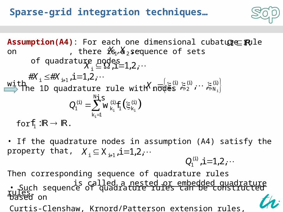
Sparse-grid integration techniques…

Assumption(A4): For each one dimensional cubature rule on , there is a sequence of sets of quadrature nodes

with

The 1D quadrature rule with nodes is

i , i 1, 2, X i i 1, i 1, 2, #X #X

i

(i) (i) (i)i 1 2 N, , , X

i i

i

N(i) (i) (i)1 k 1 k

k 1

w f Q

for 1f : .

1 2 ,X ,X

• If the quadrature nodes in assumption (A4) satisfy the property that,

Then corresponding sequence of quadrature rules is called a nested or embedded quadrature rules.

i i 1X ,i 1,2, X (i)1 , i 1, 2, Q

• Such sequence of quadrature rules can be constructed based on Curtis-Clenshaw, Krnord/Patterson extension rules, etc .

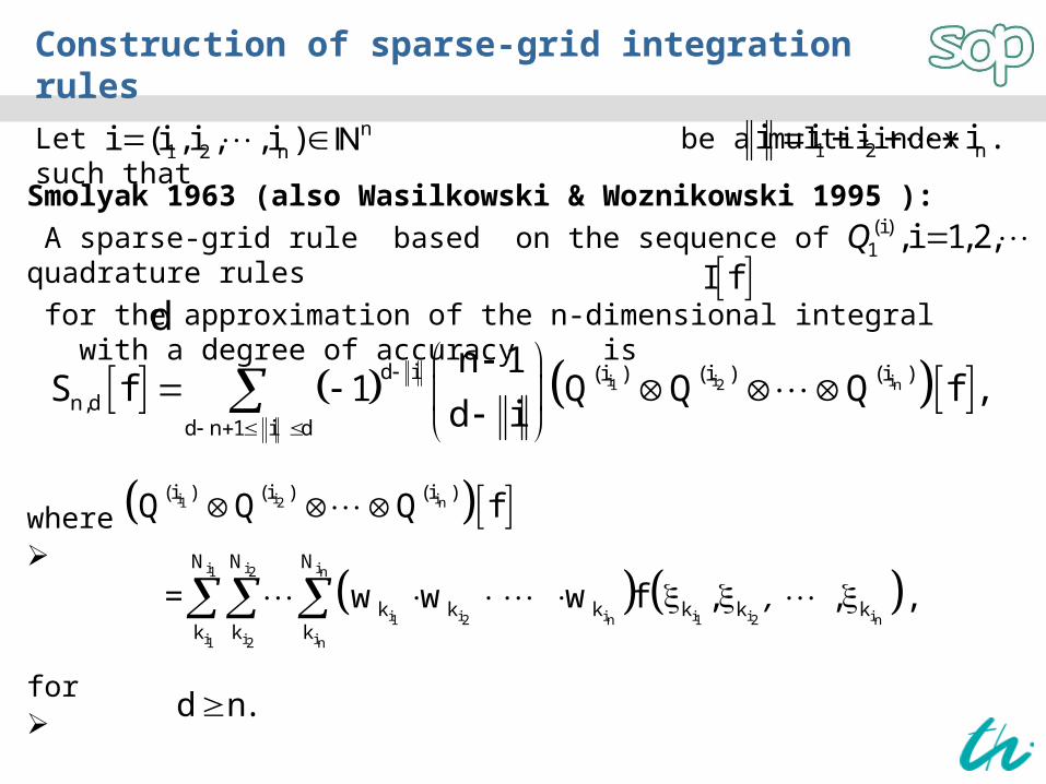
Construction of sparse-grid integration rules

Smolyak 1963 (also Wasilkowski & Woznikowski 1995 ): A sparse-grid rule based on the sequence of quadrature rules for the approximation of the n-dimensional integral with a degree of accuracy is

where

for

I f

i i i1 2 nd i (i ) (i ) (i )

n,dd n 1 i d

n 1S f 1 Q Q Q f ,

d i

(i)1 , i 1, 2, Q

d

Let be a multi-index such that n1 2 ni (i , i , , i ) 1 2 ni i i i .

i i i1 2 n

i i i1 2 n

i i i i i i1 2 n 1 2 n

i i i1 2 n

(i ) (i ) (i )

N N N

k k k k k kk k k

Q Q Q f

w w w f , , , = ,

d n.

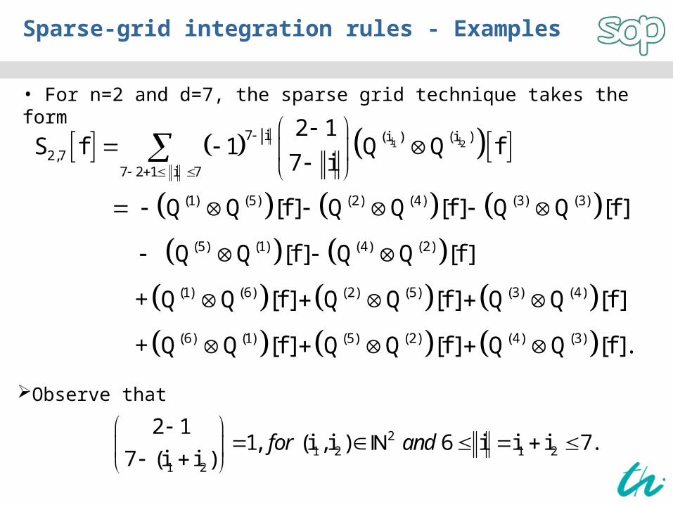
Sparse-grid integration rules - Examples

• For n=2 and d=7, the sparse grid technique takes the form

i i1 27 i (i ) (i )

2,77 2 1 i 7

(1) (5) (2) (4) (3) (3)

(5) (1) (4) (2)

(1) (6) (2) (5) (3) (4)

2 1S f 1 Q Q f

7 i

Q Q [f ] Q Q [f ] Q Q [f ]

Q Q [f ] Q Q [f ]

Q Q [f ] Q Q [f ] Q Q [

+

(6) (1) (5) (2) (4) (3)

f ]

Q Q [f ] Q Q [f ] Q Q [f ]. +

21 2 1 2

1 2

2 11, (i , i ) 6 i i i 7.

7 (i i ) for and

Observe that

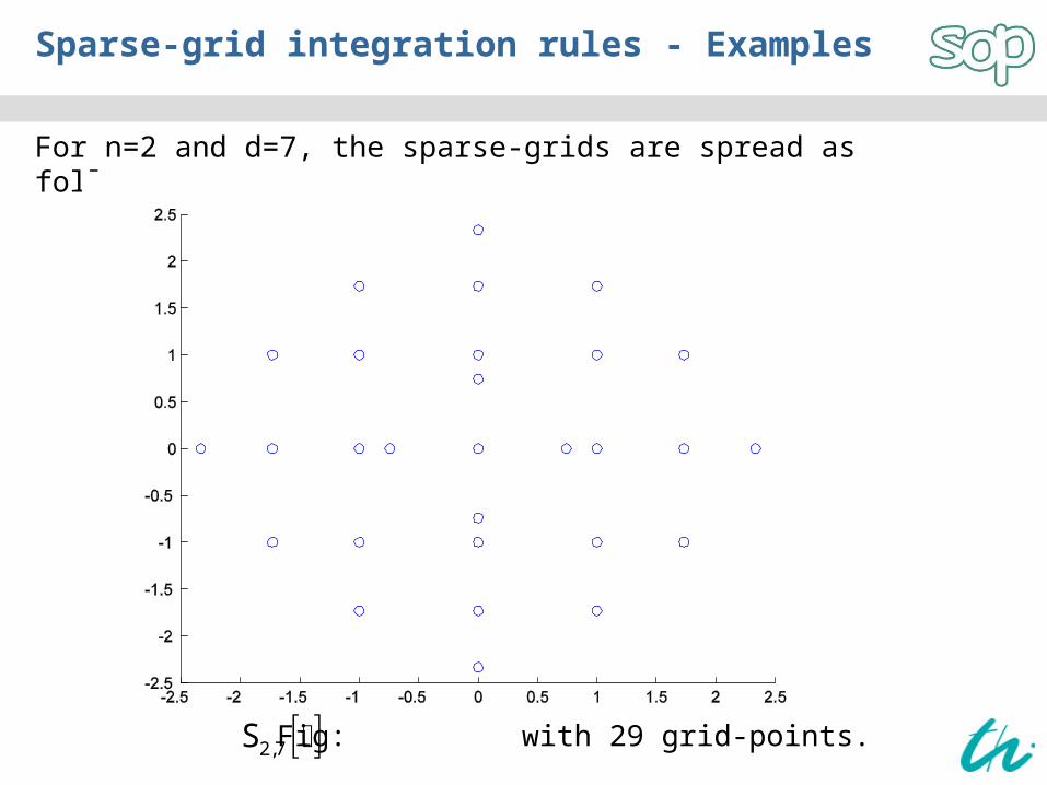
Sparse-grid integration rules - Examples

For n=2 and d=7, the sparse-grids are spread as follows:

Fig: with 29 grid-points. 2,7S

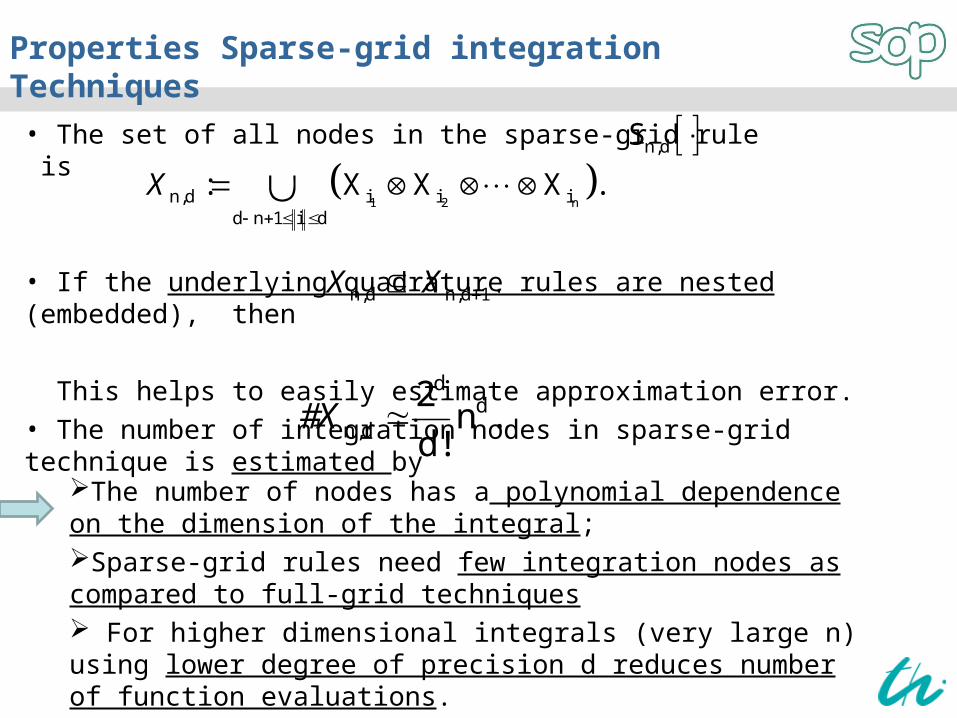
Properties Sparse-grid integration Techniques

• The set of all nodes in the sparse-grid rule is

• If the underlying quadrature rules are nested (embedded), then This helps to easily estimate approximation error.• The number of integration nodes in sparse-grid technique is estimated by

1 2 nn,d i i i

d n 1 i d

: X X X . X

n,dS

dd

n,d

2n .

d! #X

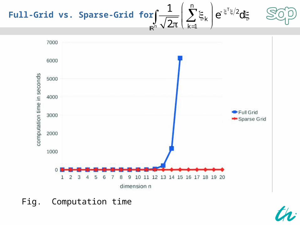
The number of nodes has a polynomial dependence on the dimension of the integral;Sparse-grid rules need few integration nodes as compared to full-grid techniques For higher dimensional integrals (very large n) using lower degree of precision d reduces number of function evaluations.

n,d n,d 1. X X

Full-Grid vs. Sparse-Grid for

Fig. Number of grid-points per dimension

T

n

n2

kk 1

1e d

2

Full-Grid vs. Sparse-Grid for

Fig. Computation time

T

n

n2

kk 1

1e d

2

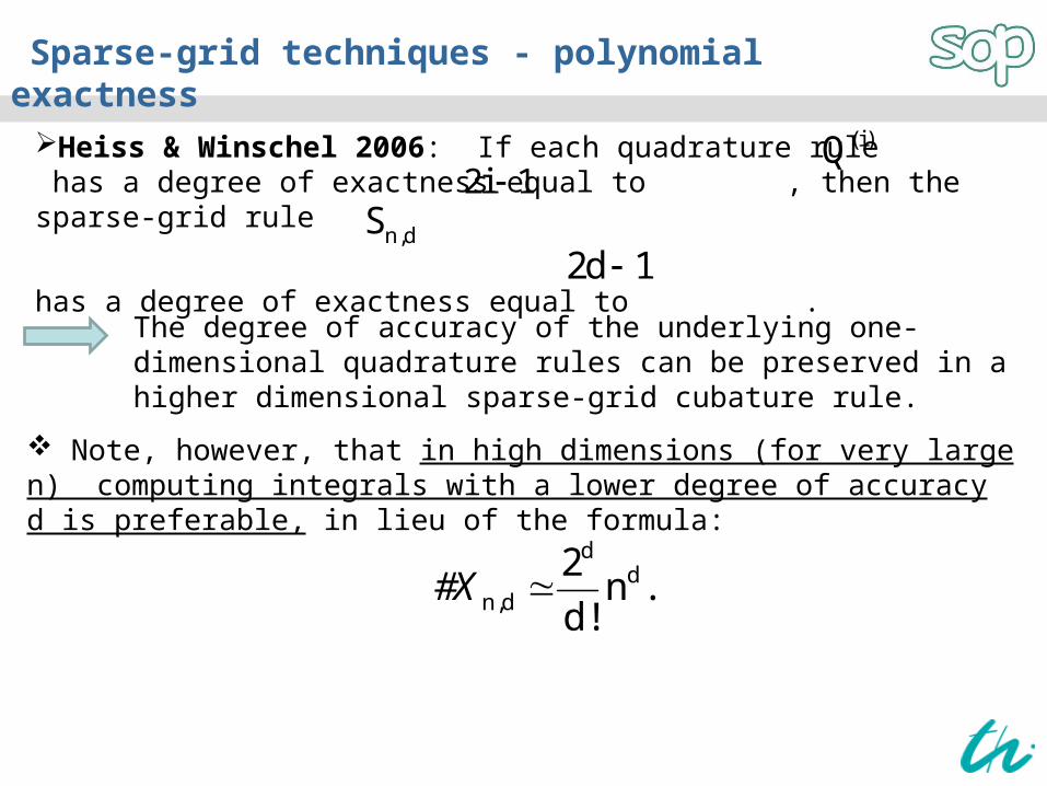
Sparse-grid techniques - polynomial exactness

Heiss & Winschel 2006: If each quadrature rule has a degree of exactness equal to , then the sparse-grid rule

has a degree of exactness equal to .

2i 1(i)Q

n,dS2d 1

The degree of accuracy of the underlying one-dimensional quadrature rules can be preserved in a higher dimensional sparse-grid cubature rule.

dd

n,d

2n .

d! #X

Note, however, that in high dimensions (for very large n) computing integrals with a lower degree of accuracy d is preferable, in lieu of the formula:

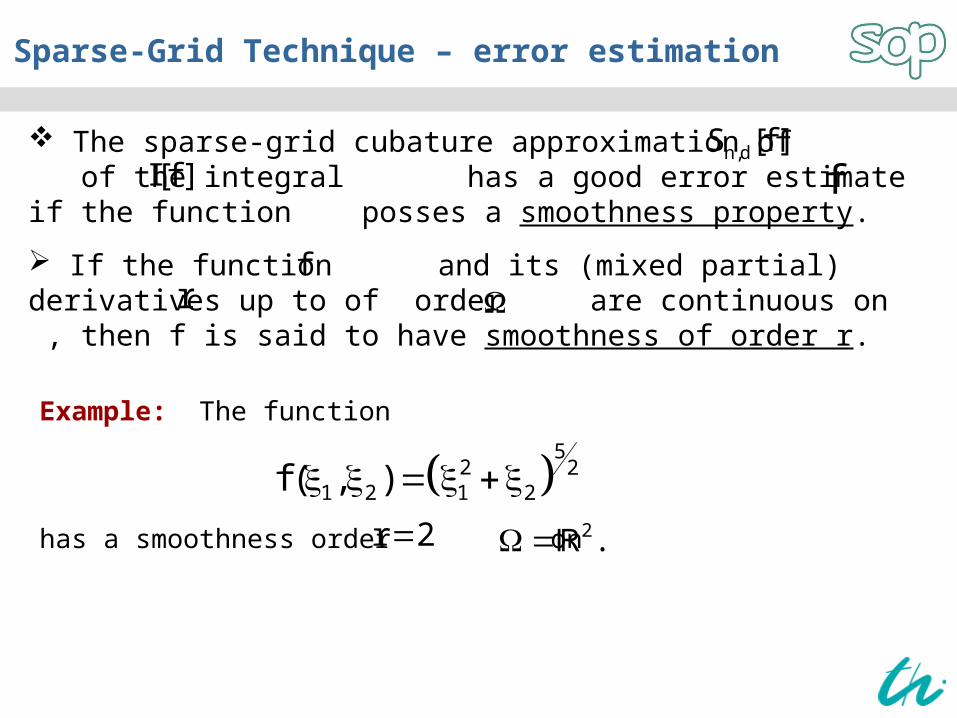
Sparse-Grid Technique – error estimation

The sparse-grid cubature approximation of of the integral has a good error estimate if the function posses a smoothness property.

If the function and its (mixed partial) derivatives up to of order are continuous on , then f is said to have smoothness of order r.

n,dS [f ]I[f ] f

fr

Example: The function

has a smoothness order on

5

2 21 2 1 2f ( , )

r 2 2.

Sparse-Grid Technique – Error estimation

Wasilkowski & Wozniakowski 1995: The error for the

approximation of by is given by

where is the number of nodes used in .

Observe that error estimation depends heavily on the factor .

I[f ] n,dS [f ]

r (n 1)(r 1)n,dI S O N (log N)

n,dS [f ]N

rN

Sparse-grid cubature rules are good approximation of multidimensional integrals if the integrand has a higher order of smoothness . r.

For integrands of lower order of smoothness, a good sparse-grid approximation requires a large number of integration nodes.

N

Ref: Wasilkowski , Wozniakowski:Explicit cost bounds of algorithms of multivariate tensor product problems.

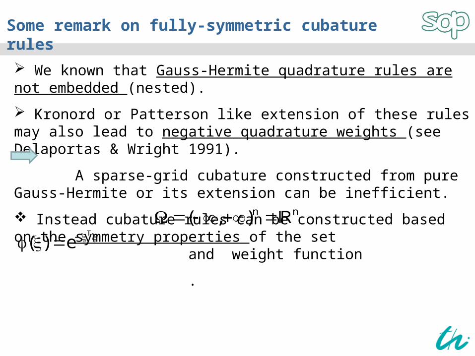
Some remark on fully-symmetric cubature rules

We known that Gauss-Hermite quadrature rules are not embedded (nested).

Kronord or Patterson like extension of these rules may also lead to negative quadrature weights (see Delaportas & Wright 1991).

A sparse-grid cubature constructed from pure Gauss-Hermite or its extension can be inefficient.

Instead cubature rules can be constructed based on the symmetry properties of the set and weight function

.

n n( , ) T

( ) e

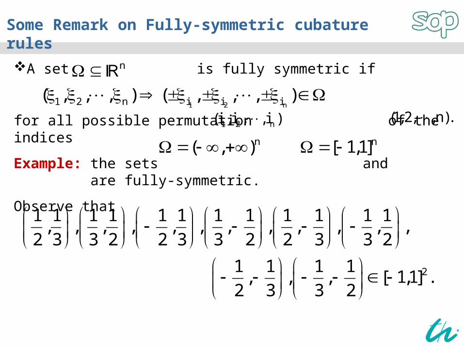
Some Remark on Fully-symmetric cubature rules

A set is fully symmetric if

for all possible permutation of the indices

Example: the sets and are fully-symmetric.

Observe that

n

1 2 n1 2 n i i i( , , , ) ( , , , ) 1 2 n(i , i , , i ) (1,2, , n).

n( , ) n[ 1,1]

2

1 1 1 1 1 1 1 1 1 1 1 1, , , , , , , , , , , ,

2 3 3 2 2 3 3 2 2 3 3 2

1 1 1 1, , , [ 1,1] .

2 3 3 2

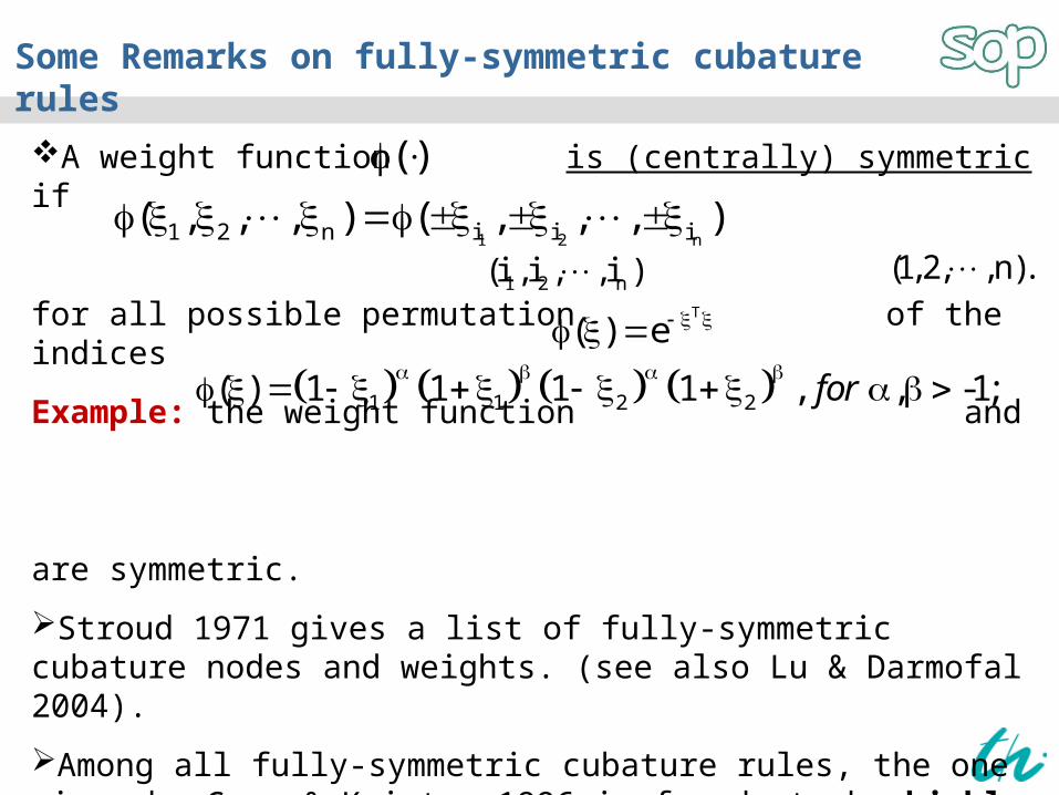
Some Remarks on fully-symmetric cubature rules

A weight function is (centrally) symmetric if

for all possible permutation of the indices

Example: the weight function and

are symmetric.

Stroud 1971 gives a list of fully-symmetric cubature nodes and weights. (see also Lu & Darmofal 2004).

Among all fully-symmetric cubature rules, the one given by Genz & Keister 1996 is found to be highly efficient for the computation of integrals with Gaussian weight functions. These are found to be sparse-grid rules with few number of nodes (Henriches & Novak 2008)

( )

1 2 n1 2 n i i i( , , , ) ( , , , ) 1 2 n(i , i , , i ) (1,2, , n).

T

( ) e

1 1 2 2( ) 1 1 1 1 , , -1; for

Advantages and Disadvantages of Sparse-Grid Integration Techniques

Advantages

The number of nodes have a polynomial (instead of exponential) dependence on the dimension of the integral;

Sparse-grid rules need few integration nodes as compared to full-grid techniques

reducing function evaluations for probability integrals

For higher dimensional integrals (very large n) using lower degree of precision d reduces number of function evaluations.

Integrals of polynomial functions can be computed exactly.

Sparse-grid integration – advantages, disadvantages

Even if the underlying quadrature rules have non-negative weights the sparse-grid cubature rule can have negative weights

the sparse-grid approximation of may not be convex w.r.t. u even if is a convex function of u.

(Convexity is vital in optimization. Convexity preserving sparse-grid techniques need further studies).

Sparse-grid integration techniques show poor performance or may even provide wrong results if the integrand is discontinuous. Also require intensive computation if the integrand has lower order of smoothness.

In fact, for discontinuous integrands, Monte-Carlo or Quasi-Monte-Carlo methods are highly preferable.

Disadvantages :

n,dS

E f (u, )f ( , )

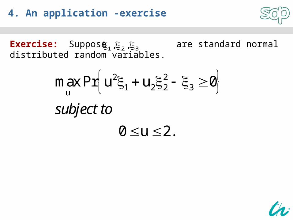
4. An application -exercise

Exercise: Suppose are standard normal distributed random variables.

1 2 3, ,

2 21 2 2 3

umax Pr u u 0

0 u 2.

subject to

5. Conclusions

There is no single general technique for the numerical computation of multidimensional integrals.

Stochastic optimization algorithms are highly dependent on the evaluation of probability integrals. Efficient techniques with a degree of accuracy in evaluating integrals greatly reduce computation time.

Dimension-adaptive sparse-grid integration techniques may provide better results.

Sparse-grid rules with positive weights are highly demanding for probability integrals

Many fully- symmetric integration techniques use a few nodes, but they are not computationally accurate.

Still there is a lot of work to be done!!

Resources

Resources for quadrature and sparse-grid integration techniques Alan Genz : http://www.math.wsu.edu/faculty/genz/software/software.html Walter Gautschi:http://www.cs.purdue.edu/archives/John Burkardt :http://people.sc.fsu.edu/~jburkardt/Sparse Grid Interpolation Toolbox:http://www.ians.uni-stuttgart.de/spinterp/Quadrature on sparse grids:

http://sparse-grids.de/

References

A. Geletu, M. Klöppel, A. Hoffmann, P. Li, Monotony analysis and sparse-grid integration for nonlinear chance constrained process optimization, Engineering Optimization, 2010.

Cools, R. Advances in multidimensional integration. J. Comput. Appl. Math. 149(2002) 1-12. Davis, P. J.; Rabinowitz, P. Methods of numerical integration. Dover Publications, 2nd

ed., 2007. Gander, M. J.; Karp, A. H. Stable computation of high order Gauss quadrature rules

using discretization for measures in radiation transfer. J. of Molecular Evolution, 53(4-5):47.

Gautschi, W. Orthogonal Polynomials: Computation and Approximation. Oxford University Press, 2004.

Genez, A. Fully symmetric interpolatory rules for multiple integrals. SIAM J. Numer. Anal., 23(1986), 1273 – 1283.

Genez, A.; Keister, B. D. Fully symmetric interpolatory rules for multiple integrals over infinite regions with Gaussian weights. J. Comp. Appl. Math., 71(1996) 299 – 309.

Gerstner, T., Griebel, M. Numerical integration on sparse grids. Numerical Algorithms, 18(1998), 209 - 232.

G. H. Golub and J. H. Welsch, Calculation of Gauss Quadrature Rules, Math. Comp., 23(1969), 221–230.

Heiss, F., Winschel, V. Esitimation with numerical integration on sparse grids. Münchner Wirtschaftswissenschaftliche Beiträge(VWL), 2006-15.

References

Hinrichs, A.; Novak, E. Cubature formula for symmetric measures in high dimensions with few points. Math. Comput. 76(2007) 1357 –1372.

Kronord, A. S. Nodes and weights of quadrature formulas. Consultants Bureau, New York, 1965.

Laurie, D. P. Calculation of Gauss-Kronord quadrature rules. Math. Comp. 66(1997) 1133 – 1145.

Lu, J.; Darmofal, D. L. Higher-dimensional integration with Gaussian weight for applications in probabilistic design. SIAM J. Sci. Comput., 26(2004) 613 – 624.

Möller, H. M. Kubaturformeln mit minimaler Knotenzahl. Numer. Math. 25(1976) 185 – 200.

Mysovskikh, I. P. On the construction of cubature formulas with the smallest number of nodes. Soviet Math. Dokl. 9(1968) 277 –280.

Patterson, T. N. L. The optimum addition of points to quadrature formulae. Math. Comp. 22(1968) 847 – 856. Errata: Math. Comp. 23(1969) 892.

Smolyak, S. A. Quadrature and interpolation formulas for tensor products of certain classes of functions. Soviet Math. Dokl., 4(1963) 240 – 243.

Stroud, A. H. Approximate calculation of multiple integrals. Printc-Hall Inc., Englewood Cliffs, N. J., 1971.

Trefethen, L. N. Is Gauss Better than Clenshaw-Curtis? SIAM Review 50(2008) 67 – 87.

Wasilkowski, G.W.; Woznikowski, H. Explicit cost bounds of algorithms for multivariate tensor product problems. J. Complexity, 11(1995), 1 – 56.

References

Wendt, M., Li, P., Wozny, G. Nonlinear chance-constrained process optimization under uncertainity. Ind. Eng. Chem. Res., 41(2002.), 3621 – 3629.

Welcome to Ilmenau !

Many thanks for your attention !