INTEGRATION OF CONTROL THEORY AND SCHEDULING METHODS FOR SUPPLY CHAIN MANAGEMENT by Kaushik Subramanian A dissertation submitted in partial fulfillment of the requirements for the degree of Doctor of Philosophy (Chemical and Biological Engineering) at the UNIVERSITY OF WISCONSIN–MADISON 2012 Date of final oral examination: 12/19/12 The disseration is approved by the following members of the Final Oral Committee: James B. Rawlings, Professor, Chemical and Biological Engineering Christos T. Maravelias, Associate Professor, Chemical and Biological Engineering Micheal D. Graham, Professor, Chemical and Biological Engineering Ross E. Swaney, Associate Professor, Chemical and Biological Engineering Jennifer Reed, Assistant Professor, Chemical and Biological Engineering Ananth Krishnamurthy, Associate Professor, Industrial and Systems Engineering
Transcript
INTEGRATION OF CONTROL THEORY AND SCHEDULING METHODS FOR SUPPLY CHAIN
MANAGEMENT
by
Kaushik Subramanian
A dissertation submitted in partial fulfillment of
the requirements for the degree of
Doctor of Philosophy
(Chemical and Biological Engineering)
at the
UNIVERSITY OF WISCONSIN–MADISON
2012
Date of final oral examination: 12/19/12
The disseration is approved by the following members of the Final Oral Committee:
James B. Rawlings, Professor, Chemical and Biological Engineering
Christos T. Maravelias, Associate Professor, Chemical and Biological Engineering
Micheal D. Graham, Professor, Chemical and Biological Engineering
Ross E. Swaney, Associate Professor, Chemical and Biological Engineering
Jennifer Reed, Assistant Professor, Chemical and Biological Engineering
Ananth Krishnamurthy, Associate Professor, Industrial and Systems Engineering
2.5 (Left) Closed-loop response (Right) Warm start rendered infeasible for actual state
because of disturbance. The warm start is infeasible if V β
N (x, v) > V . . . . . . . . . . . 44
2.6 (Left) Closed-loop response. Notice that we reset the state around t = 15 (Right)Warm start rendered infeasible for actual state because of disturbance . . . . . . . . . 44
4.4 Inventories and orders placed in the supply chain: Order-up-to policy (dec: decen-tralized, ncoop: noncooperative, coop: cooperative, cent: centralized). . . . . . . . . . 102
4.5 Inventories and orders placed in the supply chain: Inventory position control (dec:decentralized, ncoop: noncooperative, coop: cooperative, cent: centralized). . . . . . 103
4.7 (Left) Closed-loop response. Notice that we reset the state t = 14, t = 24 when the costis such that the warm start is feasible for the actual state (Right) Warm start renderedinfeasible for actual state because of disturbance . . . . . . . . . . . . . . . . . . . . . . 105
5.10 Periodic production schedule to respond to nominal demands . . . . . . . . . . . . . . 141
5.11 Production schedule for the MPC without terminal constraints that optimized (5.34)(Top) compared with production schedule for the MPC with terminal constraintsthat optimized (5.36). Note how larger batches are made for the problem with termi-nal constraints . . . . . . . . . . . . . . . . . . . . . . . . . . . . . . . . . . . . . . . . . . 141
A supply chain is a network of facilities and distribution options that performs the functions
of procuring raw materials, transforming them to products and distributing the finished prod-
ucts to the customers. The modern supply chain is a highly interconnected network of facilities
that are spread over multiple locations and handle multiple products. In a highly competitive
global environment, optimal day-to-day operations of supply chains is essential.
To facilitate optimal operations in supply chains, we propose the use of Model Predictive
Control (MPC) for supply chains. We develop:
• A new cooperative MPC algorithm that can stabilize any centralized stabilizable system
• A new algorithm for robust cooperative MPC
• A state space model for the chemical production scheduling problem
We use the new tools and algorithms to design model predictive controllers for supply chain
models. We demonstrate:
• Cooperative control for supply chains: In cooperative MPC, each node makes its deci-
sions by considering the effects of their decisions on the entire supply chain. We show
that the cooperative controller can perform better than the noncooperative and decen-
tralized controller and can reduce the bullwhip effect in the supply chain.
• Centralized economic control: We propose a new multiobjective stage cost that captures
both the economics and risk at a node, using a weighted sum of an economic stage cost
xi
and a tracking stage cost. We use Economic MPC theory (Amrit, Rawlings, and Angeli,
2011) to design closed-loop stable controllers for the supply chain.
• Integrated supply chain: We show an example of integrating inventory control with pro-
duction scheduling using the tools developed in this thesis. We develop simple terminal
conditions to show recursive feasibility of such integrated control schemes.
1
Chapter 1
Introduction
In today’s highly competitive market, it is important that the process industries integrate
their manufacturing processes with the downstream supply chain to maximize economic ben-
efits. For example, BASF was able to generate $10 million/year savings in operating costs by
performing a corporate network optimization (Grossmann, 2005). In recent years, Enterprise
Wide Optimization (EWO) has become an important research area for both academia and in-
dustry. Grossmann (2005) defines EWO as
An area that lies at the interface of chemical engineering (process systems engi-
neering) and operations research. It involves optimizing the operations of supply,
manufacturing (batch or continuous) and distribution in a company. The major
operational activities include planning, scheduling, real-time optimization and in-
ventory control.
In process control technologies like Model Predictive Control (MPC), feedback from the pro-
cess, in terms of measurements of the current state of the plant, is used to improve the control
performance. It has been recognized that using feedback control can be significant for supply
chain optimization. Backx, Bosgra, and Marquardt (2000) highlight the importance of consid-
ering the dynamics and feedback in process integration. They say
Future process innovation must aim at a high degree of adaptability of manu-
facturing to the increasingly transient nature of the marketplace to meet the chal-
lenges of global competition. Adaptation to changing environmental conditions
requires feedback control mechanisms, which manipulate the quality performance
2
and transition flexibility characteristics of the manufacturing processes on the ba-
sis of measured production performance indicators derived from observations of
critical process variables. This feedback can be achieved by means of two qualita-
tively completely different approaches residing on two different time scales. The
first, shorter time scale focused approach aims at the adaptation of process oper-
ations by modified planning, scheduling and control strategies and algorithms as-
suming fixed installations. The second approach attempts to achieve performance
improvements by reengineering the plant, including process and equipment, as
well as instrumentation and operation support system design.
Model predictive control is a multi-variable control algorithm which deals with operating
constraints and multi-variable interactions. MPC’s ability to handle constraints along with the
online optimization of the control problem has made it a very popular control algorithm in the
process industries (Qin and Badgwell, 2003; Morari and Lee, 1997). At the heart of MPC is a
dynamic process model that is used to predict the influence of inputs (manipulated variables)
on the process. Based on the prediction, an optimization problem is solved online, to find the
optimal control action.
In this thesis, we propose model predictive control as a general purpose tool to aid in enter-
prise wide optimization. Traditionally, decision making in the process industries follows a hier-
archical structure. At the top, the planning module uses a simplified model of the facility along
with some knowledge of the supply chain dynamics to predict production targets and material
flows. This problem is called the Planning problem. In the scheduling layer, the solution of the
planning problem is used to find a detailed schedule for the plant. This problem is called the
Scheduling problem. The Real Time Optimizer (RTO) uses the solution of the scheduling prob-
lem to find optimal set-points for the plant. Finally, the advanced controller regulates the plant
to the predicted set-points. The main contribution of this thesis is to formulate parts of the
short term planning problem (interaction of the production facility with the supply chain) and
the production scheduling problem as dynamic models (also see hybrid modeling for rolling
horizon approaches (Maravelias and Sung, 2009, Sec 4.4)), that can be “controlled” using MPC.
3
Thus, in conjunction with economic MPC (Amrit et al., 2011) that integrates the advanced con-
trol layer with the RTO; the tools developed in this thesis allows us to study the entire decision
making hierarchy in the enterprise from a predictive control point of view.
We focus on two important aspects of the supply chain. First, from an operations research
standpoint, we use MPC to coordinate orders and shipments in the supply chain to minimize
(maximize) costs (profits). Second, from a process systems engineering standpoint, we develop
tools to formulate the short term production scheduling problem as a dynamic control prob-
lem.
Overview of the thesis
Chapter 2 – Model predictive control: In this chapter, we summarize the fundamental theory
for linear MPC. We state stability theorems for centralized, suboptimal and cooperative MPC.
We then propose a cooperative MPC algorithm that is applicable to all centralized stabilizable
systems and an algorithm for robust cooperative MPC using tube-based MPC (Rawlings and
Mayne, 2009, Chapter 3).
Chapter 3 – A state-space model for chemical production scheduling: In this chapter we de-
rive a state space model for the production scheduling problem and highlight how different
scheduling disturbances can be modeled. We use ideas from MPC like the terminal region to
show how the state space model can be used in iterative scheduling.
Chapter 4 – Distributed MPC for supply chain optimization: In this chapter, we show how
to model a supply chain, and use the theory outlined in Chapter 2 to design centralized, dis-
tributed and, robust MPC for supply chains.
Chapter 5 – Economic MPC for supply chains: In this chapter, we briefly review economic
MPC theory and show how it can be tailored for supply chains. Instead of optimizing a tracking
4
objective, we show how to design economic and multiobjective optimization problems for sup-
ply chains. We conclude this chapter with an example of an integrated production scheduling–
supply chain problem solved in a rolling horizon framework.
Chapter 6 – Conclusions and future work: We end with a summary of the contributions and
recommendations for future work.
5
Chapter 2
Model predictive control
2.1 Introduction
Model Predictive Control (MPC) is an optimization based control algorithm in which a model
of the plant is used to predict the future evolution of the plant. A constrained optimization
problem is solved using these predictions to find the optimal input to the plant. In MPC, at
each sampling time, the optimizer finds the next N inputs, in which N is called the predic-
tion/control horizon. The first of these inputs is injected to the plant and the whole proce-
dure is repeated at the next sampling time, during which, the state of the plant is estimated
from measurements. In this way, the rolling horizon framework incorporates feedback. MPC
is widely used in many industries like Petrochemicals, fine chemicals, food, automotive and
aerospace, because of its ability to handle multiple inputs and outputs (MIMO controller) and
process constraints (Qin and Badgwell, 2003).
← Past
Inputs
Setpoint
Future →
u
k = 0
yOutputs
Figure 2.1: Rolling horizon optimization.
6
Model predictive control technology has two important aspects that are interconnected.
First, is the design of the online optimization problem that is solved. The design must account
for the control objectives, process constraints and dynamics. Second, is the study of the in-
jected control moves in the plant. Since only the first input of the optimal input sequence is
used, it is important to provide guarantees that the control objectives are met in the closed-
loop. Stability theory provides controller design guidelines and theoretical support to ensure
desirable closed-loop behavior by using the rolling horizon optimization framework.
This chapter is organized as follows. In Section 2.2, we provide an overview of centralized
MPC. We discuss optimal MPC in Section 2.2.2 and suboptimal MPC in Section 2.2.3. In Sec-
tion 2.3, we introduced distributed MPC; with noncooperative MPC discussed in Section 2.3.2
and cooperative MPC discussed in Section 2.3.3. An algorithm for robust cooperative control is
presented in Section 2.4. In Section 2.5, we discuss related work in the field of cooperative/ dis-
tributed MPC. Since the focus of this thesis is the application of control technology for supply
chain optimization, we focus our attention on linear models in this section. In Chapter 4, we
show that the supply chain dynamics can be described by linear models.
2.2 Centralized MPC
2.2.1 Preliminaries
We consider the linear system
x+ = Ax +Bu (2.1)
in which x ∈Rn , u ∈Rm are the states and inputs while x+ is the successor state.
The system is constrained by the state constraint x ∈ X ⊆ Rn and input constraint u ∈ U ⊂Rm .
For a given finite horizon N , we define the input sequence as u = (u(0),u(1), . . . ,u(N −1)) ∈UN . The state at time j ≥ 0 for a system starting at state x at time j = 0, under control u is given
by φ( j ; x,u). If there is no ambiguity, φ( j ; x,u) is also denoted as x( j ).
7
We define the tracking stage cost as `(x,u) = 1/2(x ′Qx +u′Ru);Q,R > 0. We define an eco-
nomic state cost `E (x,u) in Chapter 5. Without loss of generality, we assume that the MPC is
designed to track (x,u) to the origin. For systems in which the steady state is not the origin, we
can modify `(x,u) by a simple variable transformation x ← x−xs , in which xs is the steady state
of choice. We also define a terminal cost on the state, V f (x) = 1/2x ′P x,P > 0. An important
feature of the MPC online optimization problem is the terminal constraint (2.3). The setX f ⊆Xis the terminal set.
The MPC online optimization problem is now defined as:
Proposition 13. Let J (y) be continuously differentiable and strongly convex. Let Ω =Ω1 ×Ω2,
in which y1 ∈Ω1 and y2 ∈Ω2, withΩi convex, closed and compact. Then, as p →∞, the iterates
y (p) converges to the yo , in which yo is the optimal solution to optimization problem (2.34)
This proof is provided in Stewart et al. (2010). Another proof is also provided in Bertsekas
and Tsitsiklis (1989, Prop 3.9) for Gauss-Seidel algorithm which is closely related to the Jacobi
algorithm.
We now present the exponential stability of the cooperative MPC algorithm.
Theorem 14. Let Assumptions 1 – 4 and 10 hold. Choose r > 0 such that Br ⊂ X f . For any x
for which U sN (x;r ) is not empty, choose u ∈ U s
N (x;r ). Then, the origin of the closed-loop system
obtained by Algorithm 2 is exponentially stable. The region of attraction are (arbitrarily large)
compact subsets of the feasible region
XN := x | ∃u ∈ UN , s.t U s
N (x;r ) 6=∅
Proof. We show that the closed-loop system obtained by Algorithm 2 is an implementation of
suboptimal MPC and use Theorem 11 to prove exponential stability.
We note that the optimization problem (2.33) has convex constraints and a strongly convex
objective. By choice Q,R,P > 0, we know that the Hessian H (2.19) is positive definite, and
hence strongly convex. From Assumption 4, the set ZN is convex and hence the set UN (x) is
convex too. The set U sN (x;r ) is the intersection of two convex sets. Hence, by Proposition 12,
we know that if (x, u) is feasible for (2.33) then (i) all the iterates generated by the inner loop
in Algorithm 2 are feasible; implying u(p) ∈ U sN (x;r ) and, (ii) the cost at iterate p is not greater
than the cost achieved by VN (x, u); that is VN (x,u(p)) ≤VN (x, u).
By choice of u(0), we know that (x(0), u(0)) is feasible for (2.33). Therefore, (x(0),u(p)(0)) ∈ZN with VN (x(0),u(p)(0)) ≤VN (x(0), u(0)). Since u(1) is the warm start constructed from u(p)(0),
we know that it is feasible and that u(1) ∈ G(x(0),u(p)(0)). Therefore, by induction the closed-
loop obtained by Algorithm 2 belongs to the family of closed-loop solutions for which we showed
exponential stability in Theorem 11.
23
The main difference between cooperative and noncooperative MPC is that in the inner op-
timization loop of cooperative MPC, all the subsystems minimize the centralized problem, but
subject only to their inputs. Therefore, we were able to use warm start and properties of Jacobi
algorithm to establish the cost-drop properties required to prove exponential stability.
The cooperative MPC algorithm has the following key properties:
1. The nominal closed-loop is exponentially stable.
2. The subsystems need to share models and objective functions with each other.
3. There is no coordinator. At the end of every cooperative MPC iteration, the subsystems
just need to transfer information regarding their predicted inputs with each other.
4. There is no minimum number of iterations of the inner-loop that is required. Subsystems
can choose to stop after any number of iterations.
While, we used Proposition 12 to establish recursive feasibility and cost-drop of cooperative
MPC, we cannot use Proposition 13 to establish that the as p → ∞, the solution obtained by
the cooperative MPC optimizations converge to the centralized MPC optimization problem be-
cause the constraint set u = (u1,u2, . . . ,uM ) ∈U sN (x;r ) is a coupled constraint. The optimization
problem (2.33) can be written as
PN (x) :1/2
x
u
′
H
x
u
s.t. x( j ) ∈X j ∈ 0,1, . . . , N −1
u( j ) ∈U j ∈ 0,1, . . . , N −1[AN−1B AN−2B . . . B
]u ∈X f (2.35)
|u| ≤ d |x| x ∈Br
24
In the following sections, we describe methods to “decouple” the constraint set, so that, in
addition to establishing stability, we can also establish that the inner-loop optimizations con-
verge to the centralized optimal solution. Hence, we can establish that centralized optimal and
cooperative control have the same feedback solution.
In order to do so, we make the following assumptions for cooperative MPC:
Assumption 15. There are no state constraints. State constraints are enforced as soft-penalties by
tuning the Q matrix in the stage cost.
Assumption 16. The input constraint space is uncoupled. That is, the input constraint set U is
the Cartesian product of the input constraint sets of each subsystem.
U=U1 ×U2 × . . .×UM
The sets Ui are convex, closed, compact and, contain the origin in its interior.
Using Assumption 15, the state constraints in (2.35) are removed. Assumption 16 ensures
that the input constraints for subsystem i , i = 1,2, . . . , M do not affect any other subsystems’
input constraints. Although, for most practical applications, we do nor require the constraint
|u| ≤ d |x|, we can easily separate the constraint by enforcing |ui | ≤ di |x| such that∑
i di ≤ d .
Stability requirements mean that we cannot remove the stability constraint x(N ) ∈X f from
the optimization problem. In the next two sections, we briefly review two techniques to “uncou-
ple” the terminal region constraint. The advantage of using the cooperative MPC formulations
without coupled terminal constraints is that we have a “performance guarantee” that the open-
loop cost attained by the cooperative MPC algorithm if the inner-loop was allowed to converge
would be the optimal centralized open-loop cost.
25
2.3.3.1 Sub-states
This relaxation was proposed by Stewart et al. (2010), to solve the terminal equality con-
straint problem. That is X f = 0. The centralized optimization problem is 7:
PN (x) :minu
VN (x,u)
s.t. xi ( j +1) = Ai xi ( j )+Bi i ui ( j )+ ∑l∈1,2,...,M
l 6=i
Bi l ul ( j ), j = 0,1,2, . . . , N −1 , i = 1,2, . . . , M
ui ( j ) ∈Ui j = 0,1,2, . . . , N −1 , i = 1,2, . . . , M
xi (0) = xi i = 1,2, . . . , M
xi (N ) = 0 i = 1,2, . . . , M
(2.36)
Notice that the only coupled constraint is xi (N ) = 0, as the dynamics x+ = Ax +Bu can be
projected out, i.e., we use the optimization problem formulation (2.35).
We consider a non-minimal realization of the system (2.25) such that “sub-state” xi l in sub-
system i is only influenced by input l .
x+i l = Ai l xi l + Bi l ul (2.37)
7To simplify the discussion, we enforce the constraint that all the states are zero at the end of the horizon. In
Stewart et al. (2010), only the unstable states were forced to be zero at the end of the horizon
26
Defining xi =[
xi l , l = 1,2, . . . , M]
, each subsystem model is given by (2.25). The matrices
Ai , Bi l are used to describe the dynamics in subsystem i .
xi 1
xi 2
...
xi M
+
︸ ︷︷ ︸x+
i
=
Ai 1
Ai 2
. . .
Ai M
︸ ︷︷ ︸
Ai
xi 1
xi 2
...
xi M
︸ ︷︷ ︸
xi
+
Bi 1
0...
0
︸ ︷︷ ︸
Bi 1
u1 +
0
Bi 2
...
0
︸ ︷︷ ︸
Bi 2
u2 + . . .
0
0...
Bi M
︸ ︷︷ ︸
Bi M
uM (2.38)
xi =[Ci 1 Ci 2 . . . Ci M
]︸ ︷︷ ︸
Ci
xi 1
xi 2
...
xi M
︸ ︷︷ ︸
xi
(2.39)
We assume that the centralized states xi can be constructed from the sub-states xi . In gen-
eral, we would require that the outputs measured in subsystem i , yi can be reconstructed from
the sub-states (see Assumption 17).
The subsystem stage cost `i (xi ,ui ) = 1/2(x ′i Qi xi +ui Ri ui ) can now be written as
`i (xi ,ui ) = `i (xi ,ui ) = 1/2(xi C ′i QCi xi +ui Ri ui )
The centralized stage cost is `(x,u) =∑Mi=1`i (xi ,ui ). Since, we use a terminal constraint that
all states are zero at the end of the horizon, we do not need a terminal penalty.
We define x l as the sub-states that are affected by input l . That is x l =[
xi l i = 1,2, . . . , M ]
.
Correspondingly, we define Al ,B l as follows:
x1l
x2l
...
xMl
+
︸ ︷︷ ︸x+
l
=
A1l
A2l
. . .
AMl
︸ ︷︷ ︸
Al
x1l
x2l
...
xMl
︸ ︷︷ ︸
x
+
B1l
B2l
...
BMl
︸ ︷︷ ︸
B l
ul (2.40)
27
The constraint xi (N ) = 0 can be equivalently written as xi l = 0, l ∈ 1,2, . . . , M . Therefore,
the centralized MPC problem can be written as:
PN (x) :minu
VN (x,u)
s.t. x l ( j +1) = Axl ( j )+B l ( j )ul ( j ) j = 0,1,2, . . . , N −1 , l = 1,2, . . . , M
xi ( j ) = Ci xi ( j ) j = 1,2, . . . , N , i = 1,2, . . . , M
ul ( j ) ∈U j = 0,1,2, . . . , N −1 , l = 1,2, . . . , M
xi (0) = xi i = 1,2, . . . , M
x l (N ) = 0 l = 1,2, . . . , M (2.41)
In the optimization problem the terminal condition is uncoupled because the dynamics
of state x l depends only on input ul via equation (2.40). If Assumption 17 is satisfied, then
Algorithm 2 can be used to stabilize the plant with guaranteed performance to the centralized
solution of the problem (2.36) as there are no coupled constraints in the problem.
Assumption 17 ensures that (i) the input ui can be used to zero all the states that ui influ-
ences, (ii) all the substates can be reconstructed from the outputs.
Assumption 17 (Subsystem stabilizability).
• The system (Ai ,B i ) is stabilizable.
• The system (Ai ,Ci ) is detectable.
We now discuss the features of the aforementioned decomposition:
Applicability. The decomposition into the substate models (2.25) can be obtained from the
Kalman decomposition of the original input/output yi ,ui model (Antsaklis and Michel, 1997,
p.270).
The drawback however, is that not all centralized stabilizable models have a corresponding
substate non-minimal realization that satisfies Assumption 17. One such example is the system
of integrators (like supply chain models).
28
Convergence. The decomposition ensures that if the inner optimization loop in Algorithm 2
is allowed to converge, then the solution is the centralized solution to the optimization problem
(2.36).
Initialization. The optimization loop in Algorithm 2 requires an feasible starting point. The
feasible starting point is ensured by the warm start. The warm start is feasible because we as-
sume that the actual plant state at the next sampling time is equal to the model prediction
for the next state. In many cases, when there are plant-model mismatches or unmodeled dis-
turbances affecting the system, this assumption that the plant state is equal to the predicted
state might break-down. In such cases, the warm start becomes infeasible and we need an dis-
tributed initialization routine.
In the substate decomposition of the model, the warm start is infeasible if xi l (N ; x,u) 6= 0
for some i , l . However, since xi l (N ; x,u) depends only on the input sequence from a single
subsystem ul , the re-initialization routine is also decoupled.
2.3.3.2 Relaxing the terminal region
This relaxation was proposed by Rawlings, Stewart, Wright, and Mayne (2010), and has been
used for nonlinear suboptimal/ distributed / economic MPC in Stewart et al. (2011), Pannoc-
chia et al. (2011), Amrit et al. (2011) as well as linear MPC in Subramanian et al. (2012b).
In this section, we work with the centralized model (2.25). The idea here is to develop an op-
timization problem without terminal constraints such that every iterate generated in the inner
optimization loop of Algorithm 2 lies inside a terminal region that satisfies Assumption 3. To do
so, we modify (i) the terminal region (ii) the cost function and (iii) the feasible set as follows:
The terminal region is chosen as a sublevel set of the terminal cost. That is,
X f := x |V f (x) ≤ a, a > 0
(2.42)
For linear systems, we could use P , the solution to the Lyapunov equation as V f (x) and
choose a such that all the requirements in Assumption 3 are satisfied.
29
The cost function is modified so that the terminal penalty is magnified. That is,
V β
N (x,u) =N−1∑j=0
`(x(i ),u(i ))+βV f (x(N )) (2.43)
in which β≥ 1.
Finally, the feasible set is modified as follows:
Zβ
N =
(x,u) |V β
N (x,u) ≤ V ,u ∈UN
(2.44)
in which V ≥ 0 can be chosen arbitrarily large.
In Proposition 18, we show how the parameter β can be chosen so that if (x,u) ∈ ZβN , then
x(N ; x,u) ∈X f . Using Proposition 19 8, we can establish that the warm start given by Definition
8 satisfies the cost-drop property, i.e., V β
N (x, u) ≤V β
N (x,u).
Proposition 18. Let Assumption 2 hold. Define the terminal region X f according to (2.42) Let
the cost function V β
N (x,u) be given by (2.43). For V ≥ a, define β := V /a. Then, for any β ≥ β
and (x,u) ∈ZβN (2.44), we have that φ(N ; x,u) ∈X f .
Proof. For sake of contradiction, assume that (x,u) ∈ ZβN , β ≥ β, but φ(N ; x,u) ∉ X f , that is
V f(φ(N ; x,u)
)> a. Since (x,u) ∈ZβN , we know that
V β
N (x,u) =N−1∑i=0
`(φ(i ; x,u),u(i ))+βV f(φ(N ; x,u)
)≤ V
From Assumption 2, we know that `(x,u) ≥ 0, which implies that
βV f (φ(N ; x,u)) ≤ V
Since β≥ β= Va ,
V
aV f
(φ(N ; x,u)
)≤ V
which implies that V f(φ(N ; x,u)
) ≤ a, which is a contradiction. Therefore, for β ≥ β, if (x,u) ∈Zβ
N , then φ(N ; x,u) ∈X f .
8see also Rawlings and Mayne (2009, Exercise 2.11, Page 177)
30
Proposition 19. Let Assumption 2 hold. Choose terminal set X f according to 2.42, such that it
satisfies Assumption 3. Then for every β≥ 1, any x ∈X f , and u = κ f (x), the following holds:
βV f (Ax +Bκ f (x))+`(x,κ f (x)) ≤βV f (x)
Proof. From Assumption 3, we know that
V f (Ax +Bκ f (x))+`(x,κ f (x)) ≤V f (x)
Hence:
βV f (Ax +Bκ f (x))+β`(x,κ f (x)) ≤βV f (x)
From Assumption 2, `(x,κ f (x)) ≥ 0, V f (·) ≥ 0. Henceβ`(x,κ f (x)) ≥ `(x,κ f (x)) and the result
follows.
Proposition 20. Let Assumptions 2–3 hold, with the X f chosen according to (2.42). Choose
V ≥ a, β≥ β= V /a and cost function V β
N (x,u) given by (2.43). Choose (x,u) ∈ZβN . Then, for the
successor state x+ = Ax +Bu(0), with u(0) being the first input in the sequence u, choose the
warm start u according to Definition 8. Then, u ∈G(x,u), with the set G defined in Definition 9.
Proof. Since (x,u) ∈ ZβN , we can use Proposition 18 to establish that x(N ) = φ(N ; x,u) ∈ X f .
Since Assumption 3 holds, we know that the warm start is feasible. Hence V β
N (x+, u) ≤ V . By the
construction of the warm start, we have that:
VN (x+, u) =VN (x,u)+ (βV f (Ax(N )+Bu+)+`(x(N ),u+)−βV f (x(N ))
)−`(x,u(0))
The result follows from Proposition 19 and Assumption 2
The centralized MPC optimization problem is now written as:
PN (x) :minu
V β
N (x,u)
s.t. xi ( j +1) = Ai xi ( j )+Bi i ui ( j )+ ∑l∈1,2,...,M
l 6=i
Bi l ul ( j ), j = 0,1,2, . . . , N −1 , i = 1,2, . . . , M
ui ( j ) ∈Ui j = 0,1,2, . . . , N −1 , i = 1,2, . . . , M
xi (0) = xi i = 1,2, . . . , M
(2.45)
31
Notice that we do not enforce any terminal constraints in problem (2.45) because they are
automatically satisfied by the choice of β andZβN . That is, we restrict the feasible states to lie in:
Xβ
N :=
x | ∃u ∈UN s.t. (x,u) ∈ZβN
Since (2.45) is a convex problem subject to uncoupled constraints (the equality constraints
are projected out), for any (x,u) ∈ZβN , we have that
V β,0N (x,u0) ≤V β
N (x,u(p)) ≤V β
N (x,u) ≤ V
in which V β,0N (x,u0) is the optimal cost and V β
N (x,u(p)) is the cost obtained after p iterations of
Jacobi algorithm (Algorithm 3) applied to optimization problem (2.45). Also, as p →∞, u(p) ←u0. Hence Algorithm 2 can be used to stabilize the plant with guaranteed performance to the
centralized solution of the problem (2.45).
We now discuss the features of the aforementioned relaxation:
Applicability. The relaxation is applicable to any stabilizable centralized system.
Convergence. As mentioned earlier, the relaxation ensures that the inner optimization loop
of Algorithm 2 converges to the optimal solution of (2.45).
As shown in Pannocchia et al. (2011), for a fixed a, as we increase V , the set ZβN approaches
the following set:
Z= (x,u) | ∃u ∈UN ,φ(N ; x,u) ∈X f
Therefore, we could cover as much of the feasible space by increasing V .
The main drawback of the relaxation method is that the Hessian of the objective could get
ill-conditioned due to the choice of V and a.
Initialization. As mentioned in the previous section, the warm start could become infeasible.
From Proposition 18, it is clear that an infeasible warm start indicates that V β
N (x, u) > V . How-
ever, note that warm-start does not make the optimization problem (2.45) infeasible. Since the
inner loop optimizations decrease the objective values at each iteration, there is an iteration p ′
32
so that VN (x,u(p)) ≤ V for p ≥ p ′. After p ′ iterations of the inner optimization loop, we would
have ensured that the stability requirements are satisfied. The drawback is, unlike the regu-
lation problem with a feasible warm start, we cannot terminate the inner-loop optimizations
arbitrarily after any number of iterations. For small infeasibilities, we can expect the algorithm
to regain feasibility in a few iterations, but we do not have a theoretical upper-bound on the
number of iterations, p ′, required to regain feasibility.
2.3.4 Example9
The system, consists of two tanks with levels x1 and x2. The two tanks are considered as
two separate subsystems for implementing distributed MPC. Subsystem-1 controls the level x1
and has the inputs u11,u12,u13 at its disposal. The input u12 drains water from the first tank
into the second tank. Input u13 directly drains water from the first tank, but it is assumed that
manipulating input u13 is more expensive than manipulating input u12. Subsystem-2 controls
the level x2 and has the inputs u21 and u22 at its disposal. The input u21 recycles a fraction of
the water back into the first tank according to the recycle ratio r . Similar to subsystem-1, input
u22, which directly drains water out from subsystem-2, is assumed to be more expensive to
operate compared to input u21. To add some complexity, we assume that the recycle flow from
subsystem-2 to subsystem-1 introduces a further disturbance in the system,which is perfectly
modeled. This disturbance introduces water into the first tank at a rate proportional to the flow
out of the second tank through u21. Such interactions can arise when there is tight heat and
mass integration in chemical plants. The parameter r is chosen as 0.1.
The subsystem-1 model for the two-tank system is
x+1 = 1︸︷︷︸
A1
x1 +[
1 −1 −1]
︸ ︷︷ ︸B11
u11
u12
u13
︸ ︷︷ ︸
u1
+[
1+ r 0]
︸ ︷︷ ︸B12
u21
u22
︸ ︷︷ ︸
u2
(2.46)
9This example is taken from Subramanian et al. (2012b).
33
u11
(1+ r )u21 r u21
x2
x1
u12
u13u22
u21
Figure 2.2: The two-tank system.
34
The subsystem-2 model for the two-tank system is
x+2 = 1︸︷︷︸
A2
x2 +[
0 1 0]
︸ ︷︷ ︸B21
u11
u12
u13
︸ ︷︷ ︸
u1
+[−1 −1
]︸ ︷︷ ︸
B22
u21
u22
︸ ︷︷ ︸
u2
(2.47)
The overall (centralized) model of the two-tank system is the minimum realization of
x+ =A1 0
0 A2
︸ ︷︷ ︸
A
x +B11 B12
B21 B22
︸ ︷︷ ︸
B
u (2.48)
in which x = (x1, x2) and u = (u11,u12,u13,u21,u22). Each input is constrained to lie between
[0, u] in which 0 corresponds to the valve completely closed and u corresponds to the valve
completely open. The upper bound on the valve was chosen to be arbitrarily large.
We define stage costs `1(·, ·) and `2(·, ·):
`1(x1,u1) = x21 +u2
11 +u212 +100u2
13
`2(x2,u2) = x22 +u2
21 +100u222
The system starts at steady state with tank levels (7,7) and all valves closed. At time t = 0, we
change the setpoint of the two tanks to level (3,3) and all valves closed.
The responses are shown in Figure 2.3. In noncooperative MPC, each subsystem uses the
cheap input u12,u21 to change the tank levels; unaware that this choice of inputs leads to insta-
bility by introducing more water into the system. The subsystems manipulate the cheap inputs
because the influence of their inputs on the other subsystem is not captured in the noncooper-
ative MPC optimization problem. At each iteration, the two subsystems, optimizing indepen-
dently, harm each other because they do not want to operate the expensive valves u13 and u22.
In cooperative MPC, subsystem-2 realizes that operating valve u21 is not desirable, because it
optimizes the overall objective function. The subsystems now judiciously use the expensive
valves to maintain stability.
35
0
5
10
0 10 20 30
Leve
l-1
0 10 20 30
0
5
10
Leve
l-2
ncoop
coop
cent
0
2
0 10 20 30
Tan
k-1
Ch
eap
inp
ut
0 10 20 30
0
1
2
Tan
k-1
Exp
ensi
vein
pu
t
0
2
0 10 20 30
Tan
k-2
Ch
eap
valv
e
Time
0 10 20 30
0
1
2
Tan
k-2
Exp
ensi
veva
lve
Time
Figure 2.3: State and input profiles for two-tank system under distributed MPC (ncoop: nonco-
operative, coop: cooperative, cent: centralized).
36
2.4 Robust cooperative MPC
2.4.1 Preliminaries
We consider the centralized system (2.28) obtained from the distributed models (2.25), sub-
ject to bounded additive disturbance as follows:
x+ = Ax +Bu +w (2.49)
in which the inputs are assumed to lie in set ui ∈Ui as in the previous section. The assumptions
on the disturbance are stated in Assumption 21
Assumption 21 (Bounded disturbance). The additive disturbance w lies in a convex, closed and,
compact setW containing the origin in its interior.
The nominal system, without the additive disturbance is denoted as follows, using z, v for
the nominal state and input variables.
z+ = Az +B v (2.50)
At any time k, we can write the deviation between the actual state and the nominal state as
e(k) = x(k)− z(k). If the inputs to both the nominal and actual system were the same, then the
error dynamics can be written as:
e+ = Ax +Bu +w − Az +Bu = Ae +w (2.51)
Hence, given an initial e(0) = 0, the error at time k lies in the following set:
e(k) ∈ S(k) :=k−1∑j=0
A jW=W⊕ AW⊕ . . .⊕ Ak−1W (2.52)
in which A jW indicates set multiplication. That is,
A jW :=
A j w | ∀w ∈W
37
The symbol ⊕ indicates set addition. That is,
W⊕ AW := w1 +w2 | w1 ∈W, w2 ∈ AW
For stable A, it can be shown that the set S(∞) exists and is positive invariant for the system
(2.51) (Kolmanovsky and Gilbert, 1998).
2.4.2 Tube based MPC
We now discuss tube based MPC (Rawlings and Mayne, 2009, Chapter 3), the basic idea for
which is as follows: (i) use MPC on the nominal system to find v(k) = κ(z(k)), and (ii) based on
the error at time k, e(k), find the input to the plant as u(k) = v(k)+K e(k)
By design, we select a K such that AK := A +BK is Hurwitz. Such a choice implies that the
error dynamics in the closed-loop is:
e+ = x+− z+ = Ax +B v +BK (x − z)+w − Az −B v = AK e +w (2.53)
Now, since AK is stable, we can conclude that SK (∞) = ∑∞j=0 A j
KW exists and is positive in-
variant for (2.53).
The stability and convergence theorems are therefore based upon the following observa-
tions:(i) the origin is asymptotically stable for the nominal system z+ = Az +Bκ(z) by design,
(ii) the error is designed to lie in the set SK (∞) by the choice of K and input u = κ(z)+K (x − z),
and (iii) the actual state x(k);k →∞ therefore belongs to the set 0×SK (∞)
In the presence of persistent disturbance, we ensure that the states lie inside a bounded set
that we can compute offline. The name tube based MPC comes from the fact that at each time
k, the state x lies in a “tube” defined by x(k) ∈ z(k)⊕SK (∞) .
For the inputs u = v +K (x − z) to remain feasible, we need to ensure that v satisfies the
tighter constraints10:
V :=UªK SK (∞) (2.54)
10If state constraints are present, they need to be tightened as well. We do not discuss state constraints because
of Assumption 15
38
The tighter set follows from the fact that e = (x − z) ∈ SK (∞).
Evolve nominal state from z(k) to z(k +1) under input v(k)
Set input u(k) = v(k)+K (x(k)− z(k))
Evolve state from x(k) to x(k +1) under input u(k)
end
endAlgorithm 4: Robust cooperative MPC
42
u11
x2
x1
u12
w1 w2
u22
Figure 2.4: Two tank system
(u11,u12), while the second subsystem (tank-2) manipulates inputs u2 = (u22). There are two
disturbances affecting the system, w1 in the first tank and w2 in the second tank. The state
dynamics for this two tank system is given by:x1
x2
+
=1
1
x1
x2
+1 −1
0 1
u1 + 0
−1
u2 +w1
w2
We assume that the nominal value of w1,n = 0.1 and that of w2,n = 5. The set W is given by
W := w | 0 ≤ w1 ≤ 0.2,0 ≤ w2 ≤ 10.
The input constraints are given byU1 = u1 | 0 ≤ u11 ≤ 10,0 ≤ u12 ≤ 10 andU2 = u2 | 0 ≤ u22 ≤ 20.
Note that since we have a system of integrators, any level in the tank can be stabilized as
long as all the flows in the system are balanced. Therefore, we choose the steady state in the
tank as xs = (20,20) (the level in both tanks are 20). The input steady state is obtained by solving
the following optimization problem
minu
1/2u′Ru s.t. Bu =−wn ;u ∈U
in which wn is the nominal disturbance. For the choice of R = I (I denotes the identity matrix),
the input steady state is obtained as us = (3.2667,3.3667,8.3667).
43
The stage cost was chosen as `(x,u) = 1/2(0.1x ′x + u′u). We solve the MPC problem in
deviation variables, so that regulation to the origin implies regulation to the steady state men-
tioned above. Following the design procedure outlined in the previous sections, we choose (i)
V f (x) = 1/2x ′P x,κ f (x) = K x as the solution to the Riccati equation, (ii)a = 1 and the terminal
region as
x | 1/2x ′P x ≤ 1. The choice of a = 1 satisfies the requirements in Assumption 3, (iii)
V = 100, (iv) a prediction horizon of N = 15 and (v)the controller that corrects for the error
between the nominal and actual states was as K = κ f (x).
For these choice of parameters, we followed the algorithm mentioned in Rakovic et al. (2003)
to find the set V (we chose N = 200 and α = 1e − 6). Note that, since the original input set
contained no coupled inputs, the tightened set also contains no coupled inputs.
In Figure 2.5, we show the closed-loop response nominal closed-loop response of the level
in the second tank and the for cooperative MPC rejecting a persistent disturbance wk ∈W. We
also show the cost-function V β
N (z, v) and V β
N (x, v) to show that although the warm-start was
infeasible for the actual state, it was still feasible for the nominal state and hence we could
obtain the closed-loop guarantees for robust cooperative MPC. Note that, for this particular
disturbance realization, we could not reset the nominal state to the actual state.
In Figure 2.6, we show the closed-loop response using a modified version of Algorithm 4.
The modification we made are to reset the nominal state to the actual state at time k if the
following conditions are satisfied (i)The nominal state z(k) is inside Z f . (ii) The warm start v(k)
is feasible for the actual state x(k) and , (iii) The time elapsed since the last reset is greater than
T time periods (we chose T = 10)
2.5 Related Work
Cooperative MPC has evolved as an attractive architecture for distributed control because
it solves the centralized control problem, and inherits the desirable closed-loop properties of
centralized control. In the previous sections, we described cooperative MPC based on the “pri-
mal decomposition” of the centralized optimization problem. In the primal decomposition,
44
0
10
20
30
40
0 10 20 30 40 50
Leve
lin
Tan
k-2
Time
SK (∞) bound
0 2 4 6 8 10
0
100
200
300
400
500
Co
st
time
Actual
Nominal
VβN (x, v)
VβN (z, v)
V
Figure 2.5: (Left) Closed-loop response (Right) Warm start rendered infeasible for actual state
because of disturbance. The warm start is infeasible if V β
N (x, v) > V
10
20
30
0 10 20 30 40 50
Leve
lin
Tan
k-1
Time
SK (∞) bound
0 2 4 6 8 10
0
100
200
300
400
500
Co
st
Time
Actual
Nominal
VβN (x, v)
VβN (z, v)
V
Figure 2.6: (Left) Closed-loop response. Notice that we reset the state around t = 15 (Right)
Warm start rendered infeasible for actual state because of disturbance
45
the centralized optimization problem is solved directly using parallel optimization architec-
tures. Liu, Chen, Muñoz de la Peña, and Christofides (2010) also use the primal decomposi-
tion to solve the centralized optimization problem for a nonlinear process model. They use a
closed-form controller u = h(x) for which a Lyapunov function is known as a reference con-
troller to design their MPC optimization problem. Thus, they ensure that the MPC inherits the
stability properties of u = h(x). Note that u = h(x) also provides a warm start, even when the
actual and predicted states are different. However, since this stability constraint is a coupled
constraint, there can be no guarantees about the convergence of the parallel optimization rou-
tine to the optimal solution; and hence equivalence of optimal MPC and cooperative MPC if
the iterations were allowed to converge. The authors propose both a Jacobi algorithm (all sub-
systems optimize in parallel) and a Gauss-Seidel algorithm (subsystems optimize in sequence).
In comparison, in Stewart et al. (2011), the authors propose a Jacobi algorithm for nonlinear
MPC that converges to the centralized optimal solution. Since, for non-convex problems, the
Jacobi optimizations does not necessarily produce a descent direction, the authors propose a
sequential procedure to obtain a descent direction using the solutions obtained from each sub-
system. This overhead is not equivalent to implementing a coordinator as each subsystem only
calculates an objective function in the second phase of the algorithm in which a descent di-
rection is determined. Maestre, Muñoz de la Peña, Camacho, and Alamo (2011b) propose a
primal decomposition approach to cooperative MPC based on agent negotiation. The advan-
tage of their procedure is that agents need only know models of the subsystems whose inputs
affect their states. In the proposed method, each agent optimizes its local objective over all the
inputs that affect its dynamics, and share the proposed solution with other agents. The other
agents evaluate the proposal for cost-drop and constraint violation and communicate back to
the original agent making the proposal, who can then decide to accept or reject the proposal.
The authors ensure that only feasible proposals are accepted. The drawback of the proposed
architecture, however, is that (i) the agents have to solve larger optimization problems (because
they have to optimize over all the inputs that affect their state), and (ii) the convergence to
the centralized optimal solution cannot be guaranteed. Stability is guaranteed using the warm
46
start. Maestre, Muñoz de la Peña, and Camacho (2011a) use game-theoretic analysis to propose
a distributed optimization framework. In this method, each node, optimizes its local objective
over its local decisions while keeping the other subsystem decisions fixed. After completion of
the optimizations, the agents compute their local objectives for all possible combinations of
the overall system input (based on optimized solution of the agents and the warm start). Upon
sharing the objectives, the agents then select the input that minimizes the overall cost. Thus,
each agent cooperatively makes a decision. However, the proposed algorithm also fails to es-
tablish convergence to the centralized optimal on iteration. Stability is guaranteed by design
of terminal region and warm-start. Müller, Reble, and Allgöwer (2012) propose a optimization
algorithm based on each node optimizing over its local optimization problem. They use a ter-
minal region which is a sub-level set of the terminal penalty. Because of the presence of coupled
constraints, input directions are discarded if they are not feasible, based on a check made after
the optimizations. To ensure cost-drop, the centralized objectives are also evaluated after the
optimizations and inputs that do not achieve cost-drop are discarded. The model considered
by the authors had coupling introduced only via the constraints (both in the objective function
and the constraints). The authors also provide a method to define local time varying terminal
regions, so that the coupled terminal region constraint is satisfied if each subsystem satisfies its
local time varying terminal region constraint. The algorithm provided by the authors, satisfies
the requirements of the optimizer for suboptimal MPC, but again, does not give any guarantee
on convergence to the optimal solution. The requirement of decoupled dynamics is impor-
tant in problems like multi vehicle synchronization etc. Johansson, Speranzon, Johansson, and
Johansson (2006) use a primal decomposition to solve a multi-vehicle consensus problem as
a MPC problem. While the dynamics are decoupled, the consensus point, similar to terminal
equality constraint, is the complicating constraint. Unlike the MPC problems where the objec-
tives are also constrained because of the dynamics, the multi-vehicle receding horizon problem
falls into the category of uncoupled objective but coupled constraints. The author’s use a pri-
mal decomposition which generates feasible iterate that reduce the objective function value.
47
However, in order to ensure that the centralized optimal solution is achieved, the authors use a
coordinator, which is based on sub-gradient optimization to handle the coupled constraint.
A common theme in optimizing the centralized problem is that it is not easy to guarantee
convergence to the optimal solution. However, stability can be guaranteed because every iter-
ate is designed so that it reduces the cost while remaining feasible. In contrast, there are a lot of
cooperative MPC algorithms which are based on the “dual decomposition”. In the dual decom-
position, the coupled constraints are relaxed by using the Lagrangian of the optimization prob-
lem. For a fixed value of the Lagrange multipliers (also called as prices or dual variables), the
relaxed problem can be solved using parallel optimization methods as there are no complicat-
ing constraints. Upon achieving the solution to the relaxed problem, the Lagrange multipliers
are updated. The Lagrange multiplier update is usually done by a coordinator. These algo-
rithms often converge faster to the optimal solution. However, their main disadvantage is that
they are guaranteed to produce a feasible iterate only upon convergence. Since stability theory
for suboptimal MPC rely on the fact that the suboptimal iterate is feasible, cooperative MPC
algorithms using dual decomposition use stability theory based on optimal MPC to ensure sta-
bility. Therefore, a common theme in dual decomposition based cooperative MPC algorithms
are a coordinator layer and a requirement that the iterates converge.
The cooperative MPC algorithms using dual decomposition differ based on the technique
used to update the dual variables. In Cheng, Forbes, and Yip (2007), the dual variables (prices)
are updated using a sub-gradient based optimization algorithm. Sub-gradient methods are also
used in Ma, Anderson, and Borrelli (2011), Wakasa, Arakawa, Tanaka, and Akashi (2008), Mar-
cos, Forbes, and Guay (2009). Morosan, Bourdais, Dumur, and Buisson (2011) formulate the
building control problem as a MPC problem with linear objectives and use Benders decompo-
sition to solve the problem. Benders decomposition is a widely popular parallel algorithm when
by fixing the value of a complicating variable, the remaining problem can be completely sep-
arated. Scheu and Marquardt (2011) propose a dual decomposition algorithm without a coor-
dination layer. They augment the local subsystem objective function with the sensitivity of the
objectives and constraints of other subsystems to obtain updates for the dual variables along
48
with the primal variables. However, this method generates a feasible solution only upon con-
vergence. Giselsson, Doan, Keviczky, De Schutter, and Rantzer (2012), Giselsson and Rantzer
(2010) propose a dual decomposition algorithm with a stopping criteria based on the objective
value to ensure stability. They advocate the use of long prediction horizon along with results
obtained in Grüne (2009) to determine bounds on the value of the objective function so that
stability can be guaranteed. Doan, Keviczky, Necoara, Diehl, and De Schutter (2009) modified
the Han’s algorithm which is a dual decomposition based algorithm for the special structure
of the MPC problem. Although the method uses communication between directly connected
subsystems, stability is guaranteed only upon convergence. Necoara, Doan, and Suykens (2008)
use a smoothing technique to simplify the dual problem. With the smoothing technique, the
coordinator problem for finding the Lagrange multiplier updates becomes easier. The algo-
rithm also gives bounds on the number of iterations so that the optimal solution and constraint
violation are within a pre-specified limit (ε approximation of the centralized problem). Finally,
Doan, Keviczky, and De Schutter (2011), propose a primal feasible dual gradient approach, that
generates a primal feasible solution that achieves cost-drop in a finite number of iterations
based on an averaging scheme of the primal variables at each iteration.
Christofides, Scattolini, de la Peña, and Liu (2012) is a recent review of different algorithms
for distributed MPC. Necoara, Nedelcu, and Dumitrache (2011) provides an excellent overview
of the different optimization problems and parallel solution strategies that are seen in control
and estimation.
Trodden and Richards (2006, 2007) propose a tube based robust distributed MPC algorithm.
In their method, at each sampling time, only one subsystem performs optimization. The sub-
system optimizes only over its decision variables, keeping all other subsystem decisions fixed
from the previous iteration. This method is also an example of primal decomposition. Richards
and How (2004) present a robust tube-based MPC for systems with decoupled dynamics. The
coupling constraints are coupled output constraints. Their algorithm is based on the Gauss-
Seidel iterations.
49
Chapter 3
A state space model for chemical production scheduling
In Chapter 2, we discussed design of on-line optimization problems for the control of dy-
namic systems using MPC, so that the closed-loop has desirable properties like recursive feasi-
bility, asymptotic convergence. In this chapter, we employ ideas from MPC to address iterative
or rolling horizon scheduling problems. In Section 3.1, we provide an introduction to the prob-
lem that we wish to address. In Section 3.2, we give a brief background on chemical production
scheduling and associated rescheduling problems. In Section 3.3, we derive the state space
model, including four types of disturbances. In Section 3.4, we present an example illustrating
the advantages of using terminal constraints in iterative scheduling.
3.1 Introduction 1
Chemical production scheduling problems arise in a wide variety of applications, from batch
production of pharmaceuticals and fine chemicals to continuous production of bulk chemicals
and oil refining operations. To address these problems, research within the process systems en-
gineering (PSE) community has primarily focused on (i) the formulation of models for a wide
variety of scheduling problems, and (ii) the development of scheduling algorithms. In terms of
model development, the emphasis has been on the accurate representation of problems in a
range of production environments as well as the modeling of various processing characteristics
and constraints (e.g.,utility constraints, changeovers, transfer operations, etc.)(Méndez, Cerdá,
1This text appears in Section 1 of Subramanian, Maravelias, and Rawlings (2012a)
50
Grossmann, Harjunkoski, and Fahl, 2006). An aspect that has received limited attention is how
to design algorithms, based on these models, for iterative scheduling.
Chemical production is an inherently dynamic process. A schedule has to be revised when
new information becomes available (new orders, modified due dates, raw material availability
etc.), and/or production disturbances occur (e.g.,processing delays, unit breakdowns, process
unit availability, etc.). However, while some of the issues arising when scheduling is performed
iteratively have been discussed in contributions dealing with rescheduling, scheduling is still
thought of as a static open-loop problem – the goal is to obtain an optimal schedule for the cur-
rent state of the system based on current (and possibly some forecast) data. The development
of methods (models and solution algorithms) for the closed-loop problem has received no at-
tention. Another limitation of existing rescheduling methods, as we discuss in Section 3.2.2, is
that they are model specific and rely on the solution of a rescheduling model that is generated
empirically.
The goal of this paper is to address some of the aforementioned limitations employing ideas
from the area of control and model predictive control (MPC) in particular. Model predictive
control offers a natural framework for the study of dynamic problems. First, it relies on a gen-
eral representation of the underlying system, including different types of disturbances, via the
state space model. Second, it offers results with regard to the quality of the closed-loop per-
formance of various control strategies. For example, with careful design of the on-line opti-
mization problem, features such as recursive feasibility (feasibility of the optimization problem
at each sampling instance) and asymptotic stability (convergence to a set-point for the nom-
inal case) can be obtained. Interestingly, it has been shown that simple re-optimization does
not necessarily lead to good closed-loop performance, as has been assumed in the scheduling
literature.
Towards this goal, we first transform a general mixed-integer programming (MIP) schedul-
ing model into a state space model (2.1). Second, we show how common scheduling disrup-
tions can me modeled as disturbances in the state space model, and finally, we discuss how
some concepts from MPC like terminal constraints can be used in scheduling.
51
3.2 Background
3.2.1 Chemical production scheduling problems and models2
Production scheduling is one of the many planning functions in a manufacturing supply
chain. The interactions of scheduling with other functions along with capacity considerations
determine the class of scheduling problem. The interactions with demand and production
planning determine the type of scheduling problem to be solved (cyclic vs. short-term). The
types of decisions made at the scheduling level are determined by the decisions made at the
production planning level. Also, capacity constraints often determine the objective function
(e.g.,throughput maximization vs. cost minimization). Finally, input parameters to schedul-
ing (e.g.,raw material availability) are provided by other functions (Maravelias and Sung, 2009;
Maravelias, 2012; Stadtler, 2005).
In general, scheduling problems can be classified in terms of a triplet α/β/γ, where α de-
notes the production environment; β denotes the processing characteristics/constraints and
γ denotes the objective function (Pinedo, 2008). The main production environments are se-
quential, network and hybrid (Maravelias, 2012). Note that different types of processing can be
present in the same facility. Processing characteristics and constraints include setups, changeovers,
release/due times, storage constraints, material transfers, etc. Common objective functions
are the minimization of makespan, the minimization of production costs, the maximization of
throughput, and the minimization of weighted lateness.
The modeling approaches to chemical production scheduling can be classified in terms of
(Maravelias, 2012):
1. the decisions made at the scheduling level;
2. the entities used to express the scheduling model; and
3. the modeling of time.
2This text appears in Section 2.1 of Subramanian et al. (2012a)
52
In the most general case, scheduling involves three types of decisions: (i) batching (num-
ber and size of batches needed to satisfy demand); (ii) assignment of batches (or tasks) to
processing units; and (iii) sequencing and/or timing of batches (tasks) on processing units. If
the batching decisions are fixed, then scheduling problems are expressed in terms of batches
(batch-based approach). If batching decisions are made at the scheduling level, then materi-
als and material amounts are typically used to formulate the scheduling model (material-based
approach). Finally, the modeling of time includes decisions at four levels: (i) selection between
precedence and grid-based approach; (ii) if precedence-based, selection between local and
global precedences; if time-grid based, selection between common and unit specific grids; (iii)
specific assumptions regarding the precedence relationship between two tasks and the map-
ping of task onto time; and (iv) selection between discrete and continuous time representation
(Maravelias, 2012).
In this paper we assume batching, unit-task assignment and sequencing/timing decisions
are all made at the scheduling level (material-based approach). We further assume that the gen-
eral scheduling problem can be expressed in terms of production tasks, units(unary resources),
and materials. While this type of formalism has been traditionally used to express problems
in network production environment, Sundaramoorthy and Maravelias (2010) showed that it
can also be employed to represent problems in all production environments. A thorough dis-
cussion of the various scheduling problems and modeling approaches is presented in Méndez
et al. (2006).
3.2.2 Reactive scheduling3
Rescheduling, or reactive scheduling, after observing disturbances to the nominal schedule
has attracted some research attention in the past few years. Smith (1995) emphasizes the pro-
cess view of the scheduling problem and outlines the following criteria for reactive scheduling:
(i) prioritize outstanding problem; (ii) identify modifying goals; and (iii) estimate possibilities
3This text appears in Section 2.4 of Subramanian et al. (2012a).
53
for efficient and non-disruptive schedule modification. In the MIP-based approaches to reac-
tive scheduling, a nominal schedule is used in conjunction with a MIP model to react to distur-
bances. On observing a disturbance, part of the schedule which has already been implemented
is fixed and the remainder of the scheduling horizon is re-optimized using modifications to the
original model to reflect the disturbances. Such strategies were proposed by Vin and Ierapetri-
tou (2000); Janak, Floudas, Kallrath, and Vormbrock (2006); Relvas, Matos, Barbosa-Póvoa, and
Fialho (2007), among others. Novas and Henning (2010) propose a constraint programming
based approach to locally repair the nominal solution. Méndez and Cerdá (2003) also propose
a local repair solution to the schedule based on a MIP formulation that considers the current
“state” of the plant, a nominal schedule and new information. Motivated by rolling horizon op-
timization in process control, several shrinking horizon and rolling horizon approaches to the
scheduling problem have also been proposed. For instance, van den Heever and Grossmann
(2003) provide an example of a complex hydrogen pipeline, in which they divide the planning
horizon into planning periods, and for each planning period, they solve the scheduling prob-
lem in a shrinking horizon formulation. Sand and Engell (2004) solve a two stage stochastic
optimization problem to find robust schedules. They employ a moving horizon framework in
which the decisions in the current time period, the first stage decisions are implemented, while
the second stage decisions are embedded in a scenario tree for stochastic variables. Honkomp,
Mockus, and Reklaitis (1999) use an optimizer to perform the scheduling in conjunction with
a simulator to simulate stochastic scenarios. Rodrigues, Gimeno, Passos, and Campos (1996)
propose a rolling horizon reactive scheduling method in which they provide a predictive frame-
work to determine future infeasibilities that lie outside the current optimization horizon. Huer-
cio, Espuna, and Puigjaner (1995) present heuristics for rescheduling based on shifting of task
processing times and reassignment of tasks to other units. Li and Ierapetritou propose a multi-
parametric approach to rescheduling. Munawar and Gudi (2005) propose a three level decom-
position of the problem, and motivated by process control, formulate feedback and cascade
control-like solutions to reactive scheduling. Li and Ierapetritou (2008) present a review of
54
different strategies used in reactive scheduling. Verderame, Elia, Li, and Floudas (2010) also
present a review of different approaches taken in different industries.
3.3 State space scheduling model
3.3.1 General problem statement4
The scheduling problem we consider is stated as follows. We are given:
1. A set of processing tasks i ∈ I; the processing time of task i is denoted by τi , its fixed
batchsize by βi (variable batchsizes are considered in Section 3.3.6), and its production
cost by γi . Tasks that can be performed on many units are modeled as different tasks,
each one carried out only in one unit.
2. A set of equipment units j ∈ J. The subset of tasks i that can be carried out in unit j is
denoted by the set I j .
3. A set of materials k ∈ K stored in dedicated storage vessels of capacity σk . The unit inven-
tory cost of k is νk . The set of tasks i that produce/consume k is denoted by I+k /I−k . Task i
consumes/produces ρi k units of material k per unit of batchsize βi .
4. A set of shipments, l ∈ L (deliveries of feedstocks k ∈ KF ⊂ K or order for products k ∈ KP ⊂K); φl is the release (due) time of delivery (order) l ; and ζl is the amount delivered (ζl > 0)
or due (ζl < 0). Lk is the set of shipments (deliveries or orders) of material k.
Our goal is to meet the orders for the final products at the minimum total cost. Other objec-
tive functions can also be considered.
If a task has no input or output material (e.g.,when two consecutive tasks are carried out on
the same unit), dummy materials can be introduced to model the sequence of tasks. Also, if
material amounts need not be monitored (e.g.,sequential processes with fixed batchsize), then
we assume a nominal batchsize of 1 and unit conversion coefficients. Note that we use the term
material instead of state, because the latter has a different meaning in state space models. Raw
4This text appears in Section 2.2 of Subramanian et al. (2012a).
55
time-related data, τi and φl are given in regular time units (e.g.,hours), and are represented by
parameters with a tilde.
3.3.2 Scheduling MIP model5
We consider a discrete-time model, in which the time horizon η, is divided into T periods of
fixed length δ= η/T , defining t +1 time points, where period t starts(ends) at time point t −1(t )
(Shah, Pantelides, and Sargent, 1993). We use time index t ∈ T to denote both time point and
periods. Time-related data are scaled using δ and approximated so that the resulting solutions
are feasible. Specifically, processing times are rounded up, τi = dτi /δe; and release and due
times are approximated conservatively, φl = dφl /δe if γl > 0 and, φl = bφl /δc if γl < 0. We also
generate the set of shipments for material k at time t , Lkt =l ∈ Lk |φl = t
; and then calculate
the total shipment of material k at time t :
ξkt =∑
l∈Lkt
ζl , ∀k, t
The optimizing decisions are Wi ,t ∈ 0,1 which is one if task i is assigned to start on unit j at
time point t ; and Sk,t ≥ 0 , which is the inventory of material k during time period t . Any feasible
schedule should satisfy the assignment constraint (3.1) that expresses that at most one task can
be executed on a unit at a time.
∑i∈I j
t∑t ′=t−τi+1
Wi ,t ′ ≤ 1, ∀ j , t (3.1)
If we assume that the orders are satisfied on time, the following material balance gives the
inventory variables:
Sk,t+1 = Sk,t +∑
i∈I+k
ρi kβi Wi ,t−τi +∑
i∈I−k
ρi kβi Wi ,t +ξkt ≤σk , ∀k, t (3.2)
The objective function is
z = min∑i ,tγi Wi ,t +
∑k,tνk Sk,t (3.3)
5This text appears in Section 2.3 of Subramanian et al. (2012a)
56
Unit MaterialTask
TA
TB
U
τT B = 2hr, βT B = 6ton
τT A = 3hr, βT A = 4ton
B
A
RM
Figure 3.1: Simple scheduling problem
The basic scheduling model MSCH we consider consists of Equations (3.1)–(3.3), with Wi ,t ∈0,1 ,∀i , t and Sk,t ∈ [0,σk ].∀k, t .
If orders cannot be met on time (or we do not wish to meet them), then we can introduce
backorders variable and an additional equation for its calculation.
A simple problem with one unit, two tasks and three materials, and the associated data are
shown in Figure 3.1. Figure 3.2 shows a solution to this problem-a Gantt chart showing the
execution of the tasks and the inventory profiles of the three materials. We use this example
throughout this chapter to illustrate the basic ideas.
3.3.3 Inputs and states6
Since assignment variables Wi ,t are the main scheduling decisions; they are the inputs in the
state space realization of MSCH. Inventory levels Sk,t in MSCH are determined by Wi ,t and the in-
ventory balance dynamics, and hence are states. However, the variables Sk,t do not completely
describe the state of the system. Consider the solution shown in Figure 3.2. The variables WTA,2
and WTA,3 are both zero, but at t = 2, the task TA has run for one hour while at t = 3, the task TA
has run for two hours. Therefore, to completely describe the state of the system, the history of
the system should also be included in the system state. This is achieved through lifting. We de-
fine the new state variables W ni ,t to carry past decisions to t . The state variable W n
i ,t = 1 indicates
6This section corresponds to the model developed in Section 3.1 of Subramanian et al. (2012a).
57
Gantt Chart
Inventory profile
TA
TB
S A,tSB ,tSRM ,t
Wi ,t
Time2 4 6 8
WT B ,5 = 1WT A,1 = 1
Figure 3.2: Scheduling solution
that a batch of task i started at time t −n. The lifted equations are given by:
W 1i ,t+1 =Wi ,t
W ni ,t+1 = W n−1
i ,t ∀n ∈ 2,3, . . . ,τi (3.4)
Using the lifted states, the inventory balance equation (3.2) can be written as:
Sk,t+1 = Sk,t +∑
i∈I+k
ρi kβi W τii ,t +
∑i∈I−k
ρi kβi Wi ,t +ξk,t ∀k, t (3.5)
Similarly, the assignment constraint (3.1) can be written as
∑i∈I j
Wi ,t +∑i∈I j
τi−1∑n=1
W ni ,t ≤ 1 ∀ j , t (3.6)
Defining the state x(t ) =[
Sk,t ,k ∈ K, W ni ,t , i ∈ I,n ∈ 1,2, . . . ,τi
], the input u(t ) =
[Wi ,t , i ∈ I
]and the disturbance d(t ) =
[ξk,t ,k ∈ K
], we can write the scheduling model in the familiar state
space form x(k+1) = Ax(k)+Bu(k)+Bd d(k). Equations (3.4) and (3.5) express the dynamic evo-
lution of the system, and Equation (3.6) is a joint state-input constraint. The objective function
can be easily written as the sum of economic stage costs `E (x,u) = q ′x + r ′u.
The dynamic evolution, constraints and stage costs for the simple scheduling model intro-
duced in Figure 3.1 are given in Equations (3.7)–(3.9).
58
SRM
S A
SB
W 1TA
W 2TA
W 3TA
W 1TB
W 2TB
t+1
=
1
1 βTA
1 βTB
1
1
1
︸ ︷︷ ︸
A
SRM
S A
SB
W 1TA
W 2TA
W 3TA
W 1TB
W 2TB
t︸ ︷︷ ︸
x(t )
+
−βTA −βTB
1
1
︸ ︷︷ ︸
B
WTA
WTB
t︸ ︷︷ ︸
u(t )
+
1
1
︸ ︷︷ ︸
Bd
ξA
ξB
t︸ ︷︷ ︸
d(t )
(3.7)
0
0
0
0
≤
1
1
1
1 1 1
︸ ︷︷ ︸
Ex
SRM
S A
SB
W 1TA
W 2TA
W 3TA
W 1TB
W 2TB
t
+
1 1
︸ ︷︷ ︸
Eu
WTA
WTB
t
≤
σRM
σA
σB
1
(3.8)
`E (x,u) =[νRM νA νB
]︸ ︷︷ ︸
q ′
SRM
S A
SB
W 1TA
W 2TA
W 3TA
W 1TB
W 2TB
t
+[γTA γTB
]︸ ︷︷ ︸
r ′
WTA
WTB
t
(3.9)
59
3.3.4 Disturbances7
Events that can lead to rescheduling are modeled as disturbances. We have already dis-
cussed shipments as a disturbance in the previous section. In this section, we model three
disturbances, namely, task yields, task delays and unit breakdowns.
3.3.4.1 Shipments
We assume that backorders are not allowed. Therefore, the shipping schedule is fixed by
customer orders. Hence, shipments are treated as disturbances. We denote the nominal cus-
tomer demands as ξnomk,t . Shipment disturbances are deviations ξk,t from the nominal value.
That is,
ξk,t = ξnomk,t + ξk,t
3.3.4.2 Task yields
Consumption and production disturbances are used to model changes in yields and losses
during loading and unloading. We define yield disturbance variables βPi ,k,t and βC
i ,k,t to denote
deviation from the nominal production/consumption of material k by a batch of task i finish-
ing/starting at time t . For example, βPi ,k,t < 0 indicates lower yield than the nominal batch size.
The material balance equations (3.5) is now modified as :
Sk,t+1 = Sk,t +∑
i∈I+k
ρi kβi W τii ,t +
∑i∈I−k
ρi kβi Wi ,t +ξk,t +
∑i∈I+k
ρi kβPi ,k,t +
∑i∈I−k
ρi kβCi ,k,t
∀k, t
(3.10)
3.3.4.3 Task delays
We introduce disturbance variable Y ni ,t to model delays during the execution of a task. The
variable Y ni ,t = 1 when an 1-period delay (δ h) of task i occurring n periods after task i started
has been observed. The state equations (3.4) are corrected as:
7This section corresponds to the model developed in Section 3.1 of Subramanian et al. (2012a).
60
W 1i ,t+1 =Wi ,t − Yi ,t
W ni ,t+1 = W n−1
i ,t + Y ni ,t − Y n−1
i ,t , ∀i , t ,n ∈ 2,3, . . . ,τi (3.11)
Equation (3.11) essentially says that the values of states W ni ,t+1 should be the same as W n
i ,t if
there is a 1-period delay at t . The state equations (3.5) is corrected as:
Sk,t+1 = Sk,t +∑
i∈I+k
ρi kβi W τii ,t +
∑i∈I−k
ρi kβi Wi ,t +ξk,t −∑
i∈I+k
ρi kβi Y τii ,t ∀k, t (3.12)
For example, consider the situation in which the task TA was started at t = 1. Hence WTA,1 =1. The state equation (3.4), then implies that W 2
TA,3 = 1, as at t = 3, the task TA has been running
for 2 hours. If a 1-period delay is observed at time t = 3, then the variable Y 2TA,3 = 1. This means
that instead of finishing at t = 4, the task gets completed only at t = 5. Hence, for modeling pur-
pose, the task started only at time t = 2. In rescheduling literature, a new model is written with
this information, i.e., WTA,2 = 1,WTA,1 = 0. In our proposed method, such delays are handled
organically by modifying the lifted states. Equation (3.11) tells us that
W 3TA,4 = W 2
TA,3 + Y 3TA,3 − Y 2
TA,3 = 1+0−1 = 0
and
W 2TA,4 = W 1
TA,3 + Y 2TA,3 − Y 1
TA,3 = 0+1−0 = 1
Hence, we can verify that the disturbance variable Y ni ,t successfully models an 1-period delay.
3.3.4.4 Unit breakdowns
In contrast to a task delay, a unit breakdown leads to the termination of the task being exe-
cuted on the unit at the time of the breakdown. In such an event, all production in that unit is
also lost. To model a breakdown of unit j , we introduce disturbance variable Z ni ,t . The variable
Z ni ,t = 1 when a breakdown (of duration 1 period) occurring n hours after task i ∈ I j started is
observed. Unlike the previous section, we force all the lifted variables affected by the shutdown
61
to be zero as:
W 1i ,t+1 =Wi ,t − Zi ,t
W ni ,t+1 = W n−1
i ,t − Z n−1i ,t ∀i ,n ∈ 2,3, . . . ,τi (3.13)
The state equations (3.5) is corrected as
Sk,t+1 = Sk,t +∑
i∈I+k
ρi kβi W τii ,t +
∑i∈I−k
ρi kβi Wi ,t +ξk,t −∑
i∈I+k
ρi kβi Z τii ,t ∀k, t (3.14)
Finally, to ensure that no tasks are assigned to unit j if it is out of order, the constraint (3.6)
is modified as:
∑i∈I j
Wi ,t +∑i∈I j
τi−1∑n=1
W ni ,t +
∑i∈I j
τi−1∑n=1
Z ni ,t + Zi ,t ≤ 1 ∀ j , t (3.15)
A breakdown lasting multiple periods, from t to t+φ can be modeled as consecutive 1 period
breakdowns. Since the subsequent breakdowns occur while no task is executed, we introduce
an idle task IT( j )∀ j with τIT( j ) = 1 and use Z 1IT( j ),t+1 = Z 2
IT( j ),t+2 = . . . = Z 1IT( j ),t+φ = 1.
3.3.5 Final model
The final state space scheduling model includes the state evolution described by (3.16) and
the modified constraint given by (3.15).
W 1i ,t+1 =Wi ,t − Zi ,t − Yi ,t ∀i , t
W ni ,t+1 = W n−1
i ,t − Z n−1i ,t + Y n
i ,t − Y n−1i ,t ∀i , t ,n ∈ 2,3, . . . ,τi (3.16)
Sk,t+1 = Sk,t +∑
i∈I+k
ρi kβi W τii ,t +
∑i∈I−k
ρi kβi Wi ,t+ξk,t −∑
i∈I+k
ρi k
(βi (Z τi
i ,t − Y τii ,t )+βP
i ,k,t
)+ ∑
i∈I−k
ρi kβCi ,k,t
∀k, t
With the disturbance
d(t ) =[ξk,t ,k ∈ K, βP
i ,k,t ,βCi ,k,t , i ∈ I,k ∈ K, Yi ,t , Y n
i ,t , Zi ,t , Z ni ,t , i ∈ I,n ∈ 2,3, . . . ,τi
]
62
the final model can be written in the state space form. In the general case, we have u ∈ 0,1m
in which m = |I|; x ∈ Rnc × 0,1nb in which nc = |S| and nb = ∑i∈Iτi ; and d ∈ Rnd × 0,12nb in
which nd = |S|+∑k∈K |I−k |+ |I+k |. The symbol | · | denotes the cardinality of a set.
The state space formulation of the scheduling model is denoted as MMPC.
3.3.6 Extensions
The main ideas in transforming the discrete-time scheduling model MSCH to the state space
form MMPC is the identification of inputs and states, and the lifting of some decision variables
(inputs) so that the state vector completely describes the system. This idea can be applied to
any linear discrete-time model. For example, in this section, we show how variable batchsizes,
backorders and processing constraints can be modeled in the state space formulation.
3.3.6.1 Variable Batchsizes
Let Bi ,t ≥ 0 denote the batchsize of task i that starts at time t . The material balances in terms
of Bi ,t is
Sk,t+1 = Sk,t +∑
i∈I+k
ρi k Bi ,t−τi +∑
i∈I−k
ρi k Bi ,t +ξk,t (3.17)
Wi ,t B mini ≤ Bi ,t ≤Wi ,t B max
i , ∀k, t (3.18)
The parameters B mini and B max
i are the lower and upper bound on the batchsize of task i .
The scheduling model now consists of (3.1), (3.17) and (3.18). To formulate it in the state
space form, notice that variable Bi ,t is a decision, and hence an input. Since the state equation
(3.17) requires the input from t −τi , we lift the batch-size input to fully describe the state of the
system. Hence,
B 1i ,t+1 = Bi ,t (3.19)
B ni ,t+1 = B n−1
i ,t ∀i , t (3.20)
The model MMPC now consists of Equations (3.4), (3.20), (3.21) and constraints (3.6) and
(3.18).
63
Sk,t+1 = Sk,t +∑
i∈I+k
ρi k Bτii ,t +
∑i∈I−k
ρi k Bi ,t +ξk,t ∀k, t (3.21)
3.3.6.2 Backorders
If the demands cannot be met at a particular sampling time, then we model it using a back-
order/ backlog variable. Let Uk,t be the backlog of the material k during period t and Vk,t be the
shipment of material k during period t . The material balance now becomes,
Sk,t+1 = Sk,t +∑
i∈I+k
ρi k Bτii ,t +
∑i∈I−k
ρi k Bi ,t −Vk,t ∀k ∈ K, t (3.22)
while the backlog Ukt is calculated from
Uk,t =Uk,t −Vk,t +ξk,t ∀k, t (3.23)
From Equations (3.22) and (3.23), it is clear that the shipments Vk,t are the decisions, and
hence inputs while, backlogs are the states.
3.3.6.3 Processing constraints8
Processing constraints can be modeled following the same procedure. To illustrate, we con-
sider the modeling of tasks that require the consumption of utilities m ∈ M (e.g.,cooling water
and electricity) during their execution. Ifωm is the availability of utility m, andψi m is the utility
consumption of task i during its execution, then the resource constraint is written as:∑i∈Im
t∑t ;=t−τi+1
ψi mWi t ≤ωm ∀m, t (3.24)
in which Im is the set of tasks that consume resource m. Using the lifted W variables the con-
straint (3.24) can be written as∑i∈Im
Wi ,tψi m + ∑i∈Im
τi−1∑n=1
W ni ,tψi m ≤ωm ∀m, t (3.25)
In Section 3.4, we provide an additional example of modeling changeover time between two
tasks.8The text in this section appears in Subramanian et al. (2012a).
64
3.4 Illustrative Examples9
3.4.1 Nominal demand
We now present the rolling horizon optimization procedure for the simple scheduling exam-
ple that was introduced in Figure 3.1. We make the following modifications to the scheduling
problem: (i) Variable batch size (βmini = 5,βmax
i = 10), (ii) A changeover time of CHT(i , i ′) = 2h
when switching between products, and (iii) Nominal demands ξnomk,t = 1.5 ton every hour. No
backlogs are allowed.
To model the changeover time, we introduce three new binary variables Zi ,i ′,t ,Yi ,t and Xi ,t .
The binary variable Zi ,i ′,t is 1 when a changeover is effected from task i to task i ′ at time t . The
binary variable Yi ,t is 1 if the task i was started during [t−τi , t ]. The binary variable Xi ,t is 1 if the
last task to be performed in the unit before time t was i . The modified assignment equations
are given in (3.26) (for the example problem, hence j is omitted as there is only one uit)
∑i∈I
t∑t ′=t−τi+1
Wi ,t ′ +∑i ′∈Ii ′ 6=i
t∑t ′=t−CHT(i ,i ′)+1
Zi ,i ′,t ′ ≤ 1 ∀t
t∑t ′=t−τi+1
Wi ,t ′ = Yi ,t ∀t ,∀i ∈ I
Xi ,t ≥ Yi ,t ∀t ,∀i ∈ I∑i∈I
Xi ,t = 1 ∀t (3.26)
Zi ,i ′,t ≤ Xi ,t−1 ∀t ,∀i ∈ I, i ′ ∈ I, i ′ 6= i
Zi ,i ′,t ≤ Xi ′,t ∀t ,∀i ∈ I, i ′ ∈ I, i ′ 6= i
Zi ,i ′,t ≥ Xi ,t−1 +Xi ′,t −1 ∀t ,∀i ∈ I, i ′ ∈ I, i ′ 6= i
In the state space format, the variables Zi ,i ′,t and Xi ,t are the inputs. As we see in the mod-
ified assignment equation (3.26), the state of the plant is jointly described by the inputs Z ,W
and X from the previous time periods and the current input. Therefore, apart from lifting W ,
9The results in this section appears in Section 5 and Section 6.4 of Subramanian et al. (2012a).
65
we also lift Z and X .
Z 1i ,i ′,t+1 = Zi ,i ′,t Z 2
i ,i ′,t+1 = Z 1i ,i ′,t , ∀i , i ′ ∈ I, t
and
X 1i ,t = Xi ,t ∀i ∈ I, t
The variable Y is just a function of the lifted states W ni ,t and the input.
Yi ,t =τi−1∑n=1
W ni ,t +Wi ,t
The state space representation of the scheduling model, following the example in the previ-
ous section, can be written in the familiar format
x(t +1) = Ax(t )+Bu(t )+Bd d(t )
with constraints
b ≤ Ex x(t )+Euu(t ) ≤ b
and economic stage cost
`E (x(k),u(k)) = q ′x(k)+ r ′u(k)
The on-line optimization problem in its simplest form is now written as:
PN (x) :minu
N−1∑t=0
`E (x(t ),u(t ),d nom(t ))
s.t. x(t +1) = Ax(t )+Bu(t )+Bd d nom(t ), t = 0,1, . . . , N −1
b ≤ Ex x(t )+Euu(t ) ≤ b, t = 0,1, . . . , N −1 (3.27)
x(0) = x
in which N is the prediction horizon and d nom(t ) is the nominal demand, while u = (u(0),u(1), . . . ,u(N−1)).
The Gantt chart obtained by successive re-optimization of Problem (3.27) is shown in Fig-
ure 3.3. Note that there were no disturbances to the system. As it can be seen, the optimization
66
Time
0 4 8 12 16 20 24 28
t=0
t=1
t=2
5.50 10.00 − 6.50 10.00 − 9.00 − 5.00−
10.00 − 6.50 10.00 − 10.00 − 5.006.006.00
− infeasible
TA TB Setup Setup
Figure 3.3: Rescheduling leads to infeasibility when no backorders are allowed
problem becomes infeasible at t = 2. Notice that optimization problem (3.27) aims to mini-
mize the number of batches started as well as the inventory at each prediction time. Hence, it
starts a batch of 6 ton for task TA at t = 1. However, for the optimization problem at time t = 2,
there were not enough degrees of freedom to satisfy the demands observed t = 25, which was
not considered by the problem at t = 1. Hence, when solved within a rolling horizon frame-
work, Problem (3.27) does not guarantee recursive feasibility. As we show later in this section,
the problem would have remained feasible if a larger batch was started at t = 1. In the con-
trol literature, recursive feasibility is achieved by enforcing terminal conditions, as the terminal
conditions account for long term effects. To find a suboptimal infinite horizon schedule for this
problem, we solve the following periodic optimization problem given in (3.28). In the periodic
optimization problem, we enforce the condition that x(0) = x(Np ), which says that the state of
the system (including all the lifted variables) return to the starting state at the end of the period
Np . Therefore, the same schedule can be repeated at t = Np . In this way, we can find an infinite
horizon schedule in response to nominal demands.
67
U TA TA TB TB TB TA TA
time
0 4 8 12 16 19 0
invento
ry
0
5
10
15
20
25
A B
Figure 3.4: Periodic solution for the example in the absence of disturbances
PP : minu,x(0)
NP−1∑t=0
`E (x(t ),u(t ),d nom(t ))
s.t. x(t +1) = Ax(t )+Bu(t )+Bd d nom(t ), t = 0,1, . . . , N −1
b ≤ Ex x(t )+Euu(t ) ≤ b, t = 0,1, . . . , N −1 (3.28)
x(0) = x(Np )
The Gantt chart for the periodic solution is shown in Figure 3.4.
We now illustrate the use of terminal constraints on the states of the model which enable us
to retain feasibility of the scheduling problem as we roll the horizon forward. To do so, we use
the cyclic schedule found by optimization problem (3.28). Let the solution of the (3.28) be given
as (x0P (0),u0
P (0),u0P (1), . . . ,u0
P (Np −1)). For this optimal periodic solution, we can calculate the
corresponding state-evolution using the state evolution equation. Denote the states in this op-
timal periodic state evolution as
x0P (0), x0
P (1), . . . , x0P (Np −1)
. Then the optimization problem
68
with terminal constraints PTN (x) can be written as:
PTN (x) :min
u
N−1∑t=0
`E (x(t ),u(t ),d nom(t ))
s.t. x(t +1) = Ax(t )+Bu(t )+Bd d nom(t ),t = 0,1, . . . , N −1
b ≤ Ex x(t )+Euu(t ) ≤ b, t = 0,1, . . . , N −1 (3.29)
x(0) = x
x(N ) ∈ x0
P (0), x0P (1), . . . , x0
P (Np −1)
In optimization problem PTN , we enforce the condition that the terminal state be one of the
states in the optimal periodic state evolution. Therefore, the solutions to (3.29) contains long-
term information. This is because, we terminate at a state from which we can implement a
periodic solution to respond to nominal demands. The Gantt chart obtained by successive re-
optimization using problem (3.29) is shown in Figure 3.5. Due to design of the optimization
problem, we remain feasible at all times. Note that the batch of TA at t = 1 was 8 tons, because
of the information regarding future demands contained in the terminal constraint. Figure 3.6
shows the closed-loop solution over 24h.
We can use terminal constraints to reduce the computational burden in scheduling because,
as shown in Figure 3.7, we can guarantee recursive feasibility using shorter prediction horizons
also. In Figure 3.7, Problem (3.29) was solved with N = 12 and Figure 3.8 shows the closed-loop
solution over a horizon of 24h using a prediction horizon of 12h.
3.4.2 Rescheduling
In this section, we consider the same model as in Section 3.4.1, but with backlogs. That is,
we introduce shipments Vk,t and backlog Uk,t with the new state equations defined by (3.22)
and (3.23). We enforce an economic penalty on accumulating backlogs.
The following disturbances are observed: (i) Production delay of 1h at t = 6, (ii) breakdown
for 3h from t = 10 to t = 13, (iii) unloading error at t = 14 (production of B is 8ton instead of
10ton) and, (iv) demand spike at t = 16, with ξi = 0.5, that is the demand for both products were
2tons instead of the nominal demand of 1.5 ton. Figures 3.9 and 3.10 shows the closed-loop
Figure 3.8: Closed-loop solution solving (3.29) with N = 12h
71
performance for an optimizer optimizing (3.27). We can observe the rescheduling that occurs
naturally using the rolling horizon framework in Figure 3.9. For example, the batch sizes change
between t = 6 and t = 7 and t = 14 and t = 15 after the realization of disturbances. Finally, Figure
3.11 shows the closed-loop response for the same disturbances, but when the optimizer was
solving (3.29); that is, when we were enforcing terminal cyclic constraints. We observe inherent
robustness of the terminal constraint formulation as the backlogs accumulated are lesser than
the formulation without terminal constraints.
3.5 Discussion
3.5.1 Generality of the scheduling model10
Most current approaches to reactive scheduling are based on scheduling models that do
not include disturbances explicitly. Thus, when an event triggers rescheduling, an empirical
procedure is followed to modify the scheduling model so it (i) represents the new state of the
system, and (ii) accounts for the future impact of the disturbance. One advantage of the state
space model is that the same model can be directly used for rescheduling. All events that can
trigger rescheduling are modeled via disturbance variables. Thus, for a resolve it is sufficient to
fix the appropriate disturbance variables, which can be readily calculated from the observation
at the current time. No empirical model modifications are necessary.
3.5.2 Stochastic vs. deterministic approaches11
In this paper, we treat scheduling as an on-line problem; we optimize to determine a sin-
gle schedule based on current data and forecasts, and as new information becomes available
we re-optimize to determine, again, a single solution. In each re-optimization, we solve a de-
terministic problem- we do not account for the fact that some data are subject to uncertainty
that can be modeled. An alternative approach is to model the uncertainty in the events that
can trigger rescheduling, and then generate a solution that takes into account this information
10This text appears in Section 3.5.1 of Subramanian et al. (2012a)11This text appears in Section 3.5.2 of Subramanian et al. (2012a)
72
Time
0 4 8 12 16 20 24 28 32 36 40
t=5
t=6
t=7
t=9
t=10
t=11
t=13
t=14
t=15
t=16
− 10.0 10.0 − 6.50 10.00 − 7.009.50
− 10.0 10.0 − 8.00 10.00 − 5.50 5.00− 9.
− 10.0 10.0 − 9.50 10.00 − 7.00 5.009.
10.0 10.0 − 10.00 10.00 − 8.50 5.00−
− − 10.0 10.0 − 10.00 10.00 − 10.0 5.00−
− 10.0 10.0 10.0 − 10.00 8.00 7.50 − 6.00−
10.0 10.0 − 10.00 8.50 10.00 − 6.00 5.0010
10.0 − 10.00 10.00 10.00 − 6.00 5.0010.0
10.0 − 10.00 10.00 10.00 − 9.50 5.0010
− 10.00 10.00 10.00 − 9.00 5.0010.0
TA TB Delay Breakdown Setup Setup
1 hour delay observed
3 hour breakdown observed
Loading error observed
Demand spike observed
Figure 3.9: Rescheduling in the presence of disturbances
73
inven
tory
5
10
15
20
25
time
−1 3 7 11 15 19 23
ba
ck o
rder
0
5
10
15
20
A−Inv B−Inv A−BO B−BO
Figure 3.10: Inventory (Inv) and Backorder(BO) profiles in the closed-loop in the presence of
disturbances.
invento
ry
5
10
15
20
25
time
−1 3 7 11 15 19 23
back o
rder
0
5
10
15
20
A−Inv B−Inv A−BO B−BO
Figure 3.11: Inventory (Inv) and Backorder(BO) profiles in the closed-loop in the presence of
disturbances. Compare with 3.10 to notice the inherent robustness of the terminal constraint
formulation
74
(Li and Ierapetritou, 2008; Sahinidis, 2004). The obvious advantage of this so-called optimiza-
tion under uncertainty approach is that, if the model is solved effectively, then it can lead to
better solutions. The disadvantage is that most optimization under uncertainty methods are
computationally expensive, and thus cannot be used to address practical problems. Robust op-
timization methods have been proposed to address this shortcoming (Ben-Tal and Nemirovski,
2002; Verderame and Floudas, 2009); they rely on solutions that is almost as hard as the deter-
ministic problem, but leads to solutions that are conservative. The advantage of the control-
inspired approach that we follow is that the deterministic optimization problem can be solved
more effectively, which has three implications. First, it can lead to optimal (or near optimal)
solutions that are better (even when evaluated under uncertainty) than the solution that can
be obtained within the same time by a stochastic programming approach. Second, it allows
us to reschedule more frequently, thus reacting faster to disturbances and thereby resulting in
better closed-loop solution. Third, it allows us to consider longer scheduling horizons, which is
critical and can often be more important that accounting for uncertainty.
3.5.3 Types of disturbances and uncertainties12
Interestingly, the types of disturbances we have discussed correspond, when treated as stochas-
tic parameters, to different types of uncertainty. Shipment disturbances can be viewed as right-
hand side (RHS) uncertainty. Production and consumption disturbances can be viewed as left-
hand side (LHS) uncertainty, since they can be treated as uncertainties in theβi k = ρi kβi terms:
Sk,t+1 = Sk,t +∑
i∈I+(βi W n
i ,t +βPi ,k,t )ρi k +
∑i∈I−
(βi Wi ,t +βCi ,k,t )ρi k +ζk,t ∀k, t (3.30)
These are two types of uncertainty that have received the most attention in stochastic opti-
mization approaches to scheduling.
Task delays can also be treated as LHS uncertainty if the duration of a task appears only
as a LHS coefficient (in the case of fixed processing times) or as a variable defined in terms
12This text appears in Section 3.5.3 of Subramanian et al. (2012a). Equation (3.30) has been modified to remainconsistent with the notation used in this chapter
75
of stochastic parameters (in the case of variable processing times). Precedence-based mod-
els or time-grid based models with continuous modeling of time may result in stochastic opti-
mization problems which lead to LHS uncertainty. However, in discrete-time formulations, the
number of terms included in the summation in the LHS of the assignment constraint depends
on the duration of a task. Thus, in this case, the treatment of task delays through the modeling
of processing times as stochastic parameters leads to a structural type of uncertainty.
Finally, unit breakdowns lead to structural uncertainty since the constraints used to model
resource constraints should be removed or modified. Stochastic optimization approaches can-
not be used to effectively address this type of structural uncertainty because, in addition to
requiring on-the-fly reformulations of the scheduling model, task delays and unit breakdowns
lead to problems with either purely endogenous uncertainty or exogenous uncertainty with en-
dogenous observation (Colvin and Maravelias, 2008, 2010; Goel and Grossmann, 2006). For ex-
ample, the probability and the timing of a unit breakdown depends on the utilization of the
unit, which is determined by the decision maker. The proposed approach does not suffer from
this limitation.
3.5.3.1 Reverse transformation and reoptimization13
Since scheduling MIP models are computationally expensive, a potential disadvantage of
the proposed state space modeling framework is that it leads to MIP models of larger size.
For example. compared to its counterpart model, MSCH, model MMPC, has additional lifted
variables (lifted inputs W ni ,t ) and equations (3.4). However, model MMPC is not significantly
slower than MSCH. First we note that the addition of disturbance variables in Equations (3.16)
and (3.15) leads to changes in RHS constant vector b, if the optimization model is written as
maxc ′x : Ax ≤ b.x ∈ X
. In other words, they do not increase the complexity of the model. Sec-
ond, the lifting equations can be used to project out variables after the state of the system is
updated using MMPC and before reoptimization is performed. Commercial MIP solvers per-
form this type of preprocessing (variable elimination and constraint removal) automatically
13This text appears in Section 3.5.2 of Subramanian et al. (2012a)
76
(Atamtürk and Savelsbergh, 2005). Third, specific preprocessing methods can be easily devel-
oped to transform the current MMPC model (i.e. the model after the injection of disturbances at
t ) back to a model in the form MSCH. Perprocessing based on MMPC can also be used to auto-
matically detect what constraints should be removed or modified. For example. in the case of a
breakdown of unit j =U from t1 to t2, the constraint (3.15) becomes:
∑i∈I j
Wi ,t +∑i∈I j
τi−1∑n=1
W ni ,t ≤ 0 ∀t ∈ t1, . . . , t2 −1
which mathematically implies that all binary variables appearing in the LHS should be fixed
to zero and Equation (3.15) be removed from the model for j = U and t ∈ t1, . . . , t2 −1. Not
surprisingly, this is what one would do using logical arguments: if there is a breakdown in an
unit, then no tasks can be started on this unit (i.e., all binaries are set to zero), and thus the
corresponding assignment constraint can be removed. Model MMPC allows us to systematically
perform this type of reasoning. We note that our preliminary computational experience con-
firms that MMPC is computationally comparable with model MSCH.
Finally, lifting the inputs offers insights into generation of the models for rescheduling. As
we saw, the current state of the system includes past inputs from t −maxi τi to t . Hence, when
reformulating original model M SCH, we have to fix the decisions made in the last maxi τi pe-
riods. This approach has been proposed in the past (Sundaramoorthy and Maravelias, 2010).
The use of state space models and input lifting formalizes this approach and makes it easy to
write rescheudling model for any disturbance.
3.5.4 MPC tools14
The development of a state space model is a first step towards the use of MPC theory and
methods to address scheduling problems. It offers a representation of scheduling problems
with which the process control community is familiar. Since scheduling is a dynamic problem
and can be viewed as a production control problem, our hope is that the proposed framework
will enable MPC technology for scheduling problems.
14This text appears in Section 6.1 of Subramanian et al. (2012a)
77
Another outcome is that if facilitates the application of methods that have been developed
for hybrid dynamic systems consisting of both time and event driven dynamics (Bemporad and
Morari, 1999; Heemels, De Schutter, and Bemporad, 2001). Control of such systems has been
the focus of many researchers in the past decade (see (Camacho, Ramirez, Limon, Muñoz de la
Peña, and Alamo, 2010) for a review of MPC techniques for hybrid systems). At the same time,
studying this new class of problems can lead to the development of new tools for hybrid system.
The state space model can also help to bridge the gap between scheduling and control
since it allows the formulation of the integrated scheduling-control problem using a state space
model. Furthermore, the unified problem can be viewed as an economic MPC problem in
which the process economics (primarily determined by the scheduling decisions) are directly
optimized by the controller (Diehl, Amrit, and Rawlings, 2011).
More importantly. it offers a natural framework for the development of new scheduling al-
gorithms based on MPC. As mentioned in Section 3.1, scheduling is still thought of as an open-
loop problem, even though it is used in an iterative manner. As a results, concepts such as sta-
bility, recursive-feasibility, and closed-loop performance have received no attention. In Section
3.4, we showed how terminal constraints can be used to guarantee recursive feasibility.
78
Chapter 4
Distributed MPC for supply chain optimization
We propose cooperative model predictive control for supply chains in this chapter.
In Section 4.2, we provide a brief review of the different control theory based and distributed
decision making approaches to supply chain optimization and operation. In section 4.3, we de-
scribe the dynamic modeling of supply chains. In section 4.4. we implement cooperative MPC
on a single-product, two-echelon supply chain. Finally, we summarize our results in Section
4.5.
4.1 Introduction1
The supply chain is a system comprising organizations, decision makers, and technology
decision policies that is responsible for transforming raw materials into finished products that
are delivered to end customers. As expanded upon later in this paper, the supply chain is tra-
ditionally characterized by counter-current flows of information and material. Material flows
from the raw material suppliers through the production and distribution facilities to the end
customers, while information, in the form of demands and orders, flows from the end cus-
tomers upstream to the suppliers (Backx, Bosagra, and Marquardt, 1998; Beamon, 1998).
The decisions for supply chain management can be broadly classified into three categories:
strategic, tactical and operational. The strategic decisions are the long term planning decisions
that may include, among others, where to locate production facilities and warehouses, and in
which technologies to invest. On a medium time range, tactical decisions include selecting
1The text in this section appears in Section 1 of Subramanian et al. (2012b).
79
supply chain partners such as raw material suppliers, transportation companies, etc. The op-
erational decisions are the short term decisions, which are related to optimally operating the
supply chain. These decisions include planning and scheduling in the production facilities,
and distribution decisions such as inventory management, ordering and shipping policies, etc.
(Shah, 2005; Ganeshan and Harrison, 1995).
Shapiro (2004) lists the challenges in enlarging the scope of strategic planning in supply
chains. Among the listed challenges are integrating manufacturing, purchase and sales deci-
sions, multiperiod analysis and optimizing the overall supply chain profits. Stadtler (2005) is an
excellent overview paper about advanced planning in supply chains. The authors emphasize
linking organizational units to improve competitiveness of the supply chain. However, from an
operational viewpoint, they focus on advanced planning systems (APS) that uses information
and communication technology to coordinate all the flows (material, information, financial) in
the supply chain to best improve customer satisfaction.
The combined strategic and operational planning is a challenging optimization problem,
but researchers have made efforts to solve it; see, for instance, (Sabri and Beamon, 2000; Tsi-
akis, Shah, and Pantelides, 2001; You and Grossmann, 2008). The optimization problems for-
mulated for combined strategic and operational planning typically involve selecting a supply
chain network from a family of networks or a network superstructure. Recent developments in
combined strategic and operational planning, including handling of uncertainties and multi-
objective formulations, are described in the review paper (Papageorgiou, 2009).
At the operational level of the supply chain, the need for simultaneous decision making at
the manufacturing and the distribution sites to operate a coordinated supply chain has been
recognized. The focus of this chapter is on methods to achieve such simultaneous decisions.
This simultaneous decision making is also known as enterprise wide optimization (Grossmann,
2005).
Modern supply chains operate over multiple locations and products, and are highly inter-
connected. In a competitive economy, neglecting these interactions may result in lower profits.
A central coordinator who controls the supply chain can account for these interactions and
80
provide optimal operation. However, centralized coordination may not always be practical for
a supply chain as (i) different nodes may belong to different firms, (ii) there may be a conflict
of objectives among nodes (iii) information sharing may not be perfect and (iv) a centralized
decision maker is the most vital cog in a supply chain, and its failure may be catastrophic for
the supply chain. Therefore, distributed coordination structures for supply chain operation is
needed.
We focus on tailoring model predictive control (MPC) as a general purpose method for op-
timal supply chain operation. Model predictive control uses a dynamic model of the system
to predict future outcomes and solves a constrained optimization problem over the predicted
outcomes to find the best operational decisions. Therefore, it is well suited as a basis for supply
chain operation because it makes full use of the dynamic model and knowledge of the inter-
actions between the various nodes to predict and optimize an overall supply chain objective
function.
We propose cooperative MPC as a tool for coordinating supply chains as it retains the same
structure as traditional supply chains wherein each node makes its own local decisions, but
instead of optimizing the local objective functions, the nodes optimize the overall supply chain
objective function.
4.2 Literature survey2
A well defined supply chain optimization model requires a detailed dynamic description of
the supply chain and an objective function that captures all the essential costs and trade-offs
in the supply chain. Beamon (1998) classifies supply chain modeling in four broad categories:
Deterministic models where all the parameters are known, stochastic models with at least one
unknown parameter (typically demands) that follows a known probability distribution, eco-
nomic game theory based models, and simulation based models. As pointed out in (Sarimveis,
Patrinos, Tarantilis, and Kiranoudis, 2008), a majority of these models are steady-state models
based on average performance, and hence are unsuitable for dynamic analysis. In the review
2The text in this section appears in Section 2 of Subramanian et al. (2012b)
81
of dynamic models for supply chains, Riddalls, Bennett, and Tipi (2000) classify the models as
continuous time models, discrete time models, discrete event simulations, and operations re-
search (OR) based models.
The pioneering work of “industrial dynamics” awakened the control community’s interest in
supply chain optimization. The industrial dynamics models are the continuous (and discrete)
time dynamic models mentioned in (Angerhofer and Angelides, 2000). Industrial dynamics
captures the dynamics of the supply chains using differential (or difference) equations, and
therefore, control theory is a natural choice to study supply chain dynamics. In their simplest
form, these models capture inventory dynamics based on the shipments and orders leaving the
node
Ivi (k) = Ivi (k −1)− ∑j∈Dn(i )
Si j (k)+ ∑j∈Up(i )
S j i (k −τ j i )
in which Ivi (k) is the inventory in node i ∈ I at discrete time k, Dn(i ) is the set of nodes to
which node i ships material and Up(i ) is the set of nodes from which node i receives material.
The shipment delay between nodes i and j is denoted τi j , and Si j is the amount shipped by
node i to node j .
In order to compare different methods of supply chain operation, supply chain performance
has to be quantified. Beamon (1999, 1998) classify the performance measures in a supply chain
as quantitative measures like cost minimization, profit maximization, customer response time
minimization and, qualitative measures like customer satisfaction, flexibility etc. An impor-
tant performance measure that supply chain operation strives to reduce is the bullwhip effect,
which is defined as the amplification of demand fluctuations as one moves upstream in the
supply chain. It has been observed that the orders placed by a node to its upstream nodes
amplify (with respect to the customer demand) as one moves towards the supplier in a supply
chain. This effect increases the cost of operating the supply chain. It has been estimated that
a potential 30 billion dollar opportunity exists in streamlining the inefficiencies of the grocery
supply chain, which has more than 100 days of inventory supply at various nodes in its supply
chain (Lee, Padmanabhan, and Whang, 1997b,a). Among the reasons cited for the bullwhip ef-
fect is information distortion as one moves upstream in the supply chain. Information sharing
82
has been shown to alleviate the bullwhip effect and is part of industrial practice such as ven-
dor managed inventory (VMI), etc. The other reasons often cited for the bullwhip effect are: (i)
the misunderstanding of feedback, which occurs because the nodes do not understand the dy-
namics of the supply chain, and (ii) the use of local optimization without global vision, in which
each node tries to maximize its local profit without accounting for the effects of its decisions on
the other nodes in the supply chain (Moyaux, Chain-draa, and D’Amours, 2007). Centralized
operation of supply chains is best suited to mitigate bullwhip effect, as it has exact knowledge
of the dynamics and complete information.
Classical control theory
The earliest applications of control theory to supply chains involved studying the transfer
functions and developing single input single output (SISO) controllers for tracking inventory
to its targets. Frequency domain analysis was used to analyze and evaluate alternative supply
chain designs. In classical control approaches to controlling supply chain, the nodes were an-
alyzed as linear systems using Laplace and Z -transforms. In the work of Towill (1982), a block
diagram based approach to modeling a node was proposed. The single product node consisted
of two integrators to capture the dynamics of inventory and backorders, while the order rate was
the manipulated variable. The disturbance to the system, market demand, was incorporated in
a feed-forward manner in the model. Time delays were also incorporated in the model. A feed-
back control law was proposed for controlling the inventory deviations from a target inventory.
By varying some of these parameters like delay, controller gain etc., a family of models for a sin-
gle node called as the input-output based production control system (IOBPCS) can be studied
(Lalwani, Disney, and Towill, 2006). The feedback law, in its simplest form, takes the form of an
order-up-to policy, that is order up-to the inventory target, if the current inventory is below its
target. This policy can be viewed as a saturated proportional controller, although other forms of
the controller can also be studied. Upon having a control policy and after defining other system
details like delays, forecast smoothing etc, the transfer function of the node can be derived and
analyzed (Dejonckheere, Disney, Lambrecht, and Towill, 2003). White (1999); Wikner, Naim,
83
and Towill (1992) developed a PID controller without feed-forward forecasting for the node. A
review of stability analysis for the IOBPCS family of models is presented in Disney, Towill, and
Warburton (2006).
Classical control theory has also been studied for controlling the dynamics of the entire
supply chain as well. Grubbström and Tang (2000) provides a review of the input-output mod-
eling of supply chains and its analysis using Laplace transforms. Input-output modeling is the
matrix form description of the supply chain dynamics. Burns and Sivazlian (1978); Wikner,
Towill, and Naim (1991) analyzed multiechelon supply chains using the block diagram based
approach. They analyzed the effect of ordering policies, delays and information availability at
the nodes to analyze the supply chain response and bullwhip effect. Burns and Sivazlian (1978)
used Z -transforms in their approach and found that information distortion led to bullwhip ef-
fect. Wikner et al. (1991) found out that information sharing and echelon inventory policies
(in which each echelon considers inventory in all the nodes downstream to it) can mitigate
mann, Ydstie, and Tahmassebi (2000) have developed a continuous time model to describe a
supply chain. The model is similar to deterministic supply chain models but uses differential
equations to track dynamics. They simulated the model using a heuristic shipping policy and
studied the closed-loop supply chain under three different proportional controllers for plac-
ing orders. They developed controllers to track inventory, backorder or a combination of both.
The objective of the paper was to demonstrate that the model was capable of capturing the dy-
namics. Hence, they did not suggest any tuning methods for the controllers. Lin, Wong, Jang,
Shieh, and Chu (2004) presented an approach to analyze the closed-loop stability of a supply
chain and an approach for controller synthesis using a transfer function approach. The con-
troller policy and shipping policy were similar to the Perea López et al. (2001) paper. They an-
alyzed stability considering three extreme closed-loop scenarios: (i) high inventories and infi-
nite replenishment from upstream nodes (infinite production),(ii) a low inventory and infinite
replenishment from upstream nodes and (iii) limited production/supply. The effect of con-
troller gains on the bullwhip effect was also analyzed. The authors proposed a controller tuning
84
criterion based on frequency domain analysis of the Z -transfer functions. Venkateswaran and
Son (2005) also studied the supply chain response using Z -transform and derived stability con-
ditions for the supply chain. Hoberg, Bradley, and Thonemann (2007) applied linear control
theory on a two-echelon supply chain and concluded that order-up-to policy based on inven-
tory on hand can lead to instabilities. They found that the use of an echelon policy provides
the best performance. Dejonckheere, Disney, Lambrecht, and Towill (2004) studied informa-
tion enrichment where in, each node receives the final customer demand as well as the orders
placed by its downstream nodes, using a linear control theory based approach and concluded
that information enrichment is beneficial to the supply chain. Papanagnou and Halikias (2008)
used a proportional controller to place orders and analyzed the bullwhip effect by estimating
the state covariance matrix, for a supply chain responding to a random demand (modeled as a
white noise) at the retailer node.
Sarimveis et al. (2008); Ortega and Lin (2004) provide extensive reviews of classical control
approaches to supply chain design and operation.
Stochastic optimal control
Stochastic optimal control has been used to obtain ordering policies that minimize the ex-
pected costs of a node responding to random demands. We assume that the probability dis-
tribution of the demand is given. In its simplest form, the inventory control problem can be
formulated as a dynamic optimization problem. The order-up-to policy is one such policy that
is obtained by solving the dynamic optimization problem. The single node inventory control
problem can be cast as a Markov decision problem. See Puterman (2005) for details on setting
up the problem and algorithms. The order-up-to policy is optimal for independent and identi-
cally distributed demands as shown in the seminal paper by Clark and Scarf (1960). By consid-
ering set-up costs, it can be shown that the (σ,Σ),σ< Σ policy, in which the node orders Σ− Iv
whenever the inventory Iv falls below σ, is the optimal policy for an infinite horizon problem;
see for instance (Veinott, 1996; Iglehart, 1963; Federgruen and Zipkin, 1984). Optimality of sim-
ilar policies have been shown for Markovian demands (Song and Zipkin, 1993; Sethi and Cheng,
85
1997), compound Poisson and diffusion demands (Bensoussan, Liu, and Sethi, 2006), etc. These
results, derived for a single inventory holding facility, have been extended to multiechelon sys-
tems, (Federgruen, 1993; Shang and Song, 2003; Dong and Lee, 2003; Gallego and Özer, 2005;
Chen and Song, 2001)and capacitated systems; (Levi, Roundy, Shmoys, and Truong, 2008; Fed-
ergruen and Zipkin, 1986a,b), to better capture the dynamics of modern supply chains. Chen,
Drezner, Ryan, and Simchi-Levi (2000a); Chen, Ryan, and Simchi-Levi (2000b) quantify the bull-
whip effect for order-up-to policy under exponential smoothing and moving average forecasts.
We refer the readers to the books by Zipkin (2000) and Axsäter (2006) for more details.
Distributed decision making in supply chains
Supply chain decisions have traditionally been made by managers at each node. From a
decentralized operation perspective, supply chains can be analyzed using the tools of game
theory. In decentralized decision making, the payoff (profits) for each node depends not only
on its decisions, but also on the decisions made by the other nodes. Therefore, supply chain
operations can be viewed as a strategic game between the various nodes. Game theory based
analysis can be further classified into noncooperative and cooperative game theory.
In noncooperative game theory, each node simultaneously makes decisions and then the
payoff is obtained. Such games are characterized by the Nash equilibrium that is the set of
game outcomes for which no node has a unilateral incentive to move away from the outcome.
At the Nash Equilibrium, no node can increase its payoff by changing its decision while the
choices made by the other nodes remain the same. This result is attributed to Nash in his sem-
inal paper (Nash, 1951). Related to Nash equilibrium is the Stackelberg equilibrium attributed
to the mathematician von Stackelberg. In a Stackelberg game the nodes make their decisions
sequentially. We refer the reader to the excellent text by Basar and Olsder (1999) for detailed
analysis into game theory tools and methods. Leng and Parlar (2005); Cachon and Netessine
(2006) provide excellent reviews of game theoretic methods applied to supply chains.
86
If the nodes make the supply chain optimal decision in a noncooperative game, then the
supply chain is said to be coordinated (Cachon and Zipkin, 1999). One of the methods to coor-
dinate supply chains is to modify the interactions between the nodes of the supply chain (for
example, by adjusting contracts) so that each node, optimizing its local objective, makes the
globally optimal decision. For example, a two node newsvendor type supply chain can be co-
ordinated using buy-back contracts. A two node newsvendor supply chain consists of a retailer
and a supplier. The retailer faces a random demand with a known probability distribution at
each period. In order to respond to this demand, the retailer buys product from the supplier at
the beginning of the period. The supplier is assumed to ship products instantaneously. In the
buy-back contract, the supplier agrees to buy back unsold stock at the end of the season from
the retailer. The buy-back contract transfers some of the risk of maintaining inventory to the
supplier and divides the supply chain optimal profit (the centralized profit) among the part-
ners. In contrast, the performance of the wholesale (price only) contract, in which the supplier
supplies product at a wholesale price to the retailer, can be arbitrarily poor. Under wholesale
contract, the retailer takes all the risk of excess inventory and orders safely(Cachon, 2003; Ca-
chon and Zipkin, 1999). Perakis and Roels (2007) quantified the inefficiencies in the supply
chain (the ratio of the decentralized supply chain profits to that of the centralized supply chain
profits) for the price only or wholesale contracts. Moses and Seshadri (2000) showed that a two-
echelon supply chain can be coordinated only if the manufacturer agrees to share a fraction of
the holding costs of the retailer’s safety stock. Golany and Rothblum (2006) also studied linear
reward/penalty as a contract modification to induce coordination in the supply chain. Li and
Wang (2007) provide a survey of the various coordinating mechanisms. Axsäter (2001) studied
the Stackelberg game in the supply chain. Axsäter (2001) assumed that the manufacturer is the
leader in the Stackelberg game. The manufacturer minimized the system-wide costs and de-
clared its policies to the retailers. The retailers then optimized a modified cost function that
considers the policies of the manufacturer. They implemented an iterative optimization algo-
rithm such that the policies at every iterate was better than the initial policy. The authors also
noted that the iterations may not converge to the centralized solution.
87
On the other hand, cooperative game theory is a branch of game theory that studies the
benefits of coalitions. A coalition between nodes is formed when the nodes cooperate. These
studies allocate payoffs to various coalitions and these payoffs are analyzed via different tech-
niques like Shapley value (Shapley, 1997) or nucleolus (Schmeidler, 1969). Raghunathan (2003)
studied incentives for nodes to form information sharing partnerships. Leng and Parlar (2009)
studied different coalitions in a three-echelon supply chain. For example, if the manufacturer
and distribution center form a coalition, then it is assumed that the orders placed by the retailer
are known to both the nodes. Under the grand coalition, the final customer demand is shared
among all the three nodes. Leng and Parlar (2009) defined the payoff of a coalition as the cost
savings obtained when extra information due to the coalition is available to the nodes. Using
the payoff of all the possible coalitions, they studied the stability of different coalitions. The au-
thors noticed that the bullwhip effect is reduced when the manufacturer and distribution center
formed a coalition. Bartholdi and Kemahlioglu-Ziya (2005) studied a two-echelon supply chain
in which a manufacturer supplies to multiple retailers. They used the concepts of cooperative
game theory to find profit allocation rules after cooperation. Since the value allocation was in
the core of the cooperative game, it ensured that none of the participants in the coalition have
incentive to leave. Nagarajan and Sošic (2008) provide a comprehensive survey of cooperative
game theory applications to supply chains.
MPC for supply chains
Perea López, Ydstie, and Grossmann (2003) developed a detailed multi-product model in-
cluding time delays and a mixed integer model for the manufacturing facility. They modeled
the shipment rates with a “best I can do” policy that satisfies all the accumulated orders at a
given time if stocks are available; otherwise it ships all of its available stock. This model was
used for supply chain control using MPC maximize profit. They considered three cases in their
implementation: a centralized case, and two other cases that they termed “decentralized” con-
trol. In one decentralized control scheme, they optimized the mixed integer production facility
while operating the supply chain under a nominal control policy (like a proportional controller
88
for the orders). In the other decentralized control scheme, they optimized only the orders in the
supply chain subject to a nominal production schedule. The authors advocated the use of “cen-
tralized MPC”. Mestan, Türkay, and Arkun (2006) developed a supply chain model using a hy-
brid systems approach and implemented centralized, decentralized, and noncooperative MPC
as described in (Rawlings and Stewart, 2008). They compared customer satisfaction and supply
chain profit for the centralized and decentralized MPC. The objective functions were chosen
such that the retailer objective of maximizing customer satisfaction was in conflict with the ob-
jective of other nodes. Decentralized MPC had the highest customer satisfaction metric but the
supply chain operated at a loss. The bullwhip effect was high in the decentralized approach. In
centralized MPC, the supply chain found the trade-off between maximizing customer satisfac-
tion and minimizing overall supply chain costs. The centralized approach showed a small bull-
whip effect because all the shipment and order rates were determined by a central policy. The
authors also noted that the performance of noncooperative MPC was much better than the per-
formance of decentralized MPC. Dunbar and Desa (2007) solved a three-echelon, one-product
supply chain using a noncooperative MPC. They developed a bidirectionally coupled model, by
considering two types of delay: pipeline delay or the transportation delay and a first order ma-
terial delay to quantify delays in clearing backlogs. The algorithm was found to be better than
a nominal control policy. They also observed that the ordering policy was not very aggressive,
indicating that the bullwhip effect may be mitigated by distributed MPC. Seferlis and Giannelos
(2004) presented a two-layer MPC strategy for multiechelon supply chains. They used MPC to
find shipments and orders placed to other nodes, subject to a total order constraint. The total
orders placed was the manipulated variable of a PID controller to track inventory. The authors
suggest that the performance can be improved by better tuning the PID controller and suggest
a bi-level optimization problem in which the PID controller is replaced with an optimization-
based controller. Kempf (2004) and Braun, Rivera, Carlyle, and Kempf (2002) developed a model
predictive control framework for the supply chain in the semiconductor industry. They devel-
oped models that are specific to the semiconductor industry. Braun et al. (2002) implemented
decentralized MPC and studied the control performance under plant model mismatch. Kempf
89
(2004) described a two-loop optimization technique for the supply chain optimization prob-
lem. The coarse first loop optimizer is used to generate the inventory and order setpoints (ref-
erence trajectories), while the fine inner loop MPC is used to track these setpoints. Bose and
Penky (2000) also used an MPC framework. They focused on forecasting the demand signal and
studied the sensitivity of the MPC framework to fluctuations in the demand signal. Maestre, D.
Muñoz de la Peña, and Camacho (2009) proposed a cooperative MPC algorithm for a two-layer
supply chain. In their formulation, each node minimized its local objective function, not only
over its own decision space, but also over the decision spaces of the other nodes. Based on
the multiple optimal objective function values (one for each node), the algorithm determined a
consensus input. The drawback of the approach is that it is not scalable for large supply chains
with multiple nodes. Bemporad, Di Cairano, and Giorgetti (2005) showed the applications of
hybrid MPC (Bemporad and Morari, 1999) on a centralized supply chain management prob-
lem. Li and Marlin (2009) implemented robust MPC using an economic objective function on a
multiechelon supply chain.
In the following section, we show that the supply chain can be modeled as a system of inte-
grators.
4.3 Dynamic modeling of the supply chain3
A dynamic model is the heart of any feedback control algorithm. While developing a dy-
namic model of a supply chain, the components of a supply chain (like the production facility,
distributor, retailer etc.) are called as nodes. The supply chain network is the vertices or arcs,
which depict the connections between the various nodes. We assume that the network is fixed
and given to us. We denote the set of nodes by I . The nodes to which a particular node sup-
plies material are called its downstream nodes, while the nodes from which a particular node
obtains material are called its upstream nodes. The set of products handled in the supply chain
is given by P . For a particular node i ∈ I , the set P (i ) denotes the products handled by that
3This section has been modified from Section 3 of Subramanian et al. (2012b) to account for multiple productsin the supply chain. Equation (4.2) has been modified to track backorders for each downstream node separately.
90
node. For each node i ∈ I , and each product p ∈ P (i ) we define the set Up(i , p) as the set of
all nodes j ∈ I that are connected by an arc with i and are upstream to node i . These nodes
supply product p to node i . Similarly, we define the set of downstream nodes to i for products
p as Dn(i , p). For each arc in the the supply chain, material flows downstream and orders (or
information) flows upstream. The supply chain in the form of nodes and arcs is shown in Figure
4.1.
Suppliers DistibutionCenters
Production
Facility
Retailers
Information Flow
Product Flow
CU
STO
ME
RS
Figure 4.1: Supply chain as nodes and arcs.
From a classical chemical engineering perspective, each node can be modeled as two tanks,
the inventory tank and the backorder tank. The flows out of the inventory tank are the ship-
ments to the downstream nodes and the shipments from the upstream nodes make up the flow
into the inventory tank. The flows out of the backorder tank are the shipments to the down-
stream nodes, which alternatively can be viewed as the orders that have been met; the flows
into the backorder tank are the orders arriving at the node. For nodes that handle multiple
products, we have as many inventory and backorder tanks as the number of product handled
by the node. Figure 4.2 depicts the ‘tanks’ model of a node in the supply chain handling a single
product.
91
OrdersBack-
Decision Maker(policy implementer/ optimizer)
(placed to
upstream nodes)
(from upstream nodes)
(placed bydownstream nodes)
(to downstream nodes)
(Demands satisfied)
Information sharing
Inventory
Orders Orders
Shipments
Shipments
Figure 4.2: Tank analogy for modeling a node.
The states in each node i are: the inventory in the node, Ivpi∀p ∈P (i ), and the backorders
in the node, BOpi i ′∀p ∈ P (i ),∀i ′ ∈ Dn(i , p); two inputs: the shipments made to each down-
stream node j ∈ Dn(i , p), Spi j , and the orders placed to each upstream node j ∈ Up(i , p), Opi j .
The shipments coming from the upstream nodes Sp j i , j ∈ Up(i , p) and the orders arriving from
the downstream nodes Op j i , j ∈ Dn(i , p) are the disturbances arriving to the node. Denoting
discrete sample time by integer k, the dynamic equations for node i can be written as
in which τp j i is the transportation delay. We assume that there are no delays for order trans-
fers between the nodes. Denoting xi (k) =[
Ivpi (k), p ∈P (i ) BOpi j (k), p ∈P (i ), j ∈ Dn(i , p)]′
,
ui (k) =[
Spi j , p ∈P (i ), j ∈ Dn(i , p) Opi j ′ , p ∈P (i ), j ′ ∈ Up(i , p)]′
, and by using the lifting tech-
nique described in Chapter 3, the previous dynamic equations for the nodes can be written in
92
the familiar state space form for MPC applications
xi (k +1) = Ai i xi (k)+Bi i ui (k)+ ∑l∈Il 6=i
Bi l ul (4.3)
The decision maker shown in Figure 4.2 can take several different forms:
• Each decision maker can implement a simple ordering policy that depends only on the in-
coming shipments and orders. Such an ordering policy could be a PI controller to control
the inventory levels, or (σ,Σ) policies that are obtained from stochastic inventory con-
trol optimization. Such decision makers are implementations of classical control theory
approaches to supply chain control.
• Noncooperative MPC: Each decision maker can implement an MPC controller to regulate
its local states by optimizing a local objective function (for example, the profit function for
the node). The nodes can share information regarding upstream shipments, downstream
orders, etc. This form of control is termed noncooperative MPC.
• Cooperative MPC: Each decision maker can implement an MPC controller that consid-
ers the effect of the nodes’ decision on the entire supply chain (for example, each node
optimizes the supply chain profit function). The nodes still share information.
• Centralized MPC: We can replace all the decision makers at the nodes with a single deci-
sion maker at the supply chain level. This single decision maker makes decisions for all
the nodes.
The overall supply chain dynamic model is the individual node dynamic equations collected
for all nodes i ∈ I . The only required change in the node dynamic equation is for the retailer
and the production facility nodes.
93
Retailer models
For the retailer nodes i ∈R, the dynamic equations are modified as,
Ivpi (k +1) = Ivi (k)+ ∑j∈Up(i ,p)
Sp j i (k −τp j i )−Spi c (k), ∀p ∈P (i ) (4.4)
BOpi (k +1) = BOpi (k)+Dmpi c (k)−Spi c (k), ∀p ∈P (i (4.5)
in which Spi c is the shipment made by the retailer, and Dmpi c is the customer orders (de-
mands). The only disturbances in the overall supply chain model are the customer demands
d =[
Dmpi c
]′, p ∈ P (i ), i ∈ R, which drive all the flows (shipments and orders) in the supply
chain.
Production facility models
The production facility needs to be modeled separately because material conversion takes
place in this node. In multiple product supply chains, the same production facility handles
multiple products. Thus a model for the production facility needs to incorporate a scheduling
model to optimize the sequence of production. In this chapter, we assume that the production
facilities belong to the first echelon. We further assume an ideal supplier of raw materials to the
production facilities, implying that we have infinite supply of raw materials without transporta-
tion delay.
Planning models In this chapter, we shall use an “approximate production model” to model
the production facility. In the approximate production model, we replace the detailed schedul-
ing model with convex constraints that represent the feasible region of production. This idea is
similar to the process attainable region (Sung and Maravelias, 2007)-a convex region of produc-
tion quantities for which there exists some feasible schedule. The process attainable region can
be computed by using computational geometry tools (Sung and Maravelias, 2007; Maravelias
and Sung, 2009; Sung and Maravelias, 2009) or parametric programming tools (Li and Ierapetri-
tou, 2010). Let M be the set of production facility nodes. Then, for each i ∈ M , the modified
94
dynamic equations for the final products are
Ivpi (k +1) = Ivpi (k)+Spi m(k)− ∑j∈Dn(i ,p)
Spi j (k), ∀p ∈P (i )
BOpi j (k +1) = BOpi j (k)+Op j i (k)−Spi j (k), ∀p ∈P (i ),∀ j ∈ Dn(i , p) f (Si pm(k)) ≤ 0
in which Spi m are the manipulated inputs denoting production of product p during the period.
Note that, for multiproduct production facilities, each of the inputs Spi m for products p ∈ P
are coupled by the convex production feasibility constraint. The set L represents the set of
products.
f (S1i m(k),S2i p (k), . . . ,Spi m(k), . . .) ≤ 0
Scheduling models The state task network (STN) approach is probably the most popular method
to model a production facility in which multiple products are produced using shared resources
(Kondili, Pantelides, and Sargent, 1993; Shah et al., 1993). As described in Chapter 3, in STN
modeling, the final products, intermediates and raw materials are states that are processed us-
ing tasks like reactions, separation, etc. These tasks can be carried out in units capable of han-
dling multiple tasks. A detailed schedule is the sequence of operation of the tasks in the units so
that a production objective can be met at minimal cost without violating the scheduling con-
straints.
Detailed scheduling models are formulated as mixed integer linear programs (MILPs) or
mixed integer nonlinear programs (MINLPs). If we chose to model the production facility using
a detailed scheduling model, then the resulting supply chain MPC problems become mixed
integer programs. Although, research progress has been made in the theory of MIQP and hybrid
MPC (see (Bemporad and Morari, 1999)), in this chapter, we do not consider detailed scheduling
models in the formulation of the supply chain model. An example using a detailed scheduling
model is provided in Section 5.2.
95
4.3.1 Summary
In this section, we wish to bring to the readers’ attention, three salient features of the supply
chain dynamic model presented in this section.
Uncontrollable local models Controllability implies that there exist inputs that can move the
state of the system from any initial state to any final state in finite time. Examining (4.1) and (4.2)
for the inventory and backorder balance for node i , we observe that while nodes j ∈ Up(i , p) re-
spond to orders Opi j placed by node i , node i has no knowledge of the subsequent dynamics
of its own orders. Therefore, we need to provide the node some model of how its orders affect
the later shipments coming into the node. To do so in a noncooperative or decentralized con-
trol arrangement, we track another state (or output) Ippi termed the inventory position. The
dependence of orders on incoming shipments is modeled through the function g (·).
Ippi (k +1) = Ippi (k)+ ∑j∈Up(i ,p)
g (Opi j (k −τp j i ))− ∑j∈Dn(i )
Spi j (k) ∀p ∈P (i )
In the centralized control framework, the actual dynamics of the entire supply chain is available
to the decision maker, and the relationship of the orders at node i to its subsequent incom-
ing shipments is captured by the upstream nodes backorder balance equations and the supply
chain performance metric. From Section 2.3.3, we know that cooperative MPC algorithms has
complete model knowledge. Therefore, uncontrollable local models is not an issue when im-
plementing cooperative MPC for supply chains.
Unstable models The supply chain is modeled as a system of integrators whose response to
an input step change is a ramp. Such systems need to be stabilized in the closed loop, otherwise
the states can keep growing (think of it as backorders keep rising as time increases). Therefore,
we emphasize establishing closed-loop properties of the algorithms that we propose for supply
chain optimization.
96
dem1c (k)
S2p (k −τM )
Manufacturer Retailer
τT = 2
τM = 2
Node 1
S1c (k)
O12(k)
S21(k)
Node 2
S2p (k)
Figure 4.3: Two-stage supply chain.
Stabilizable centralized model We notice that all the nodes belonging to the manufacturing
facilities are controllable because we manipulate the production rates. Therefore, the manu-
facturing nodes do not require an inventory position model. Since the manufacturing facility
model has this property, the overall supply chain model is also controllable. The controllabil-
ity of the centralized model is an important feature that we use to design closed-loop stable
centralized and cooperative MPC frameworks for supply chain optimization.
4.4 Example4
We simulate the supply chain shown in Figure 4.3 in this section. The plant has produc-
tion delay of 2 time units and a transportation delay of 2 time units and a single product. For
simplicity, we drop the index on product in this section.
Production model As mentioned earlier, the production delay is 2 time units. However, we
assume that the manufacturer can start a batch of the product at every sampling time. This
assumption means that the manufacturer has two units that can execute the task of producing
the final product.
We label the retailer node 1, with the states Iv1 and BO1, the inventory and backorder at the
retailer. The retailer inputs u1 consist of orders placed and the shipments made by the retailer,
S1c and O12. We label the manufacturer node 2, with states x2 consisting of inventory Iv2 and
backorder BO2. The manufacturer inputs are the shipments made to the retailer S21 and the
production eS2m . The demand d(k) = Dm1c .
4The results this section, with the exception of Sections 4.4.2, 4.4.3 and the discussion on steady states, areslightly modified from Section 6 of Subramanian et al. (2012b) to reflect a coding error that was corrected.
97
Models We write a time invariant model for the supply chain that is also the process model
(because we assume that a batch may start at every time) by writing the inventory and backo-
rder balance equation. These model for the retailer is: Iv1
BO1
k+1︸ ︷︷ ︸
x1(k+1)
=1
1
︸ ︷︷ ︸
A1
Iv1
BO1
k︸ ︷︷ ︸
x1(k)
+−1 0
−1 0
︸ ︷︷ ︸
B11
S1c
O12
k︸ ︷︷ ︸
u1(k)
+−1 0
0 0
︸ ︷︷ ︸
B (2)22
S21
S2m
k−2︸ ︷︷ ︸
u2(k−2)
+0
1
︸︷︷︸
Bd
[Dm1c
]k︸ ︷︷ ︸
d(k)
(4.6)
The manufacturer state space is given by: Iv2
BO2
k+1︸ ︷︷ ︸
x2(k+1)
=1
1
︸ ︷︷ ︸
A2
Iv2
BO2
k︸ ︷︷ ︸
x2(k)
+−1 0
−1 0
︸ ︷︷ ︸
B22
S21
S2m
k︸ ︷︷ ︸
u2(k)
+0 1
0 0
︸ ︷︷ ︸
B (2)22
S21
S2m
k−2︸ ︷︷ ︸
u2(k−2)
+0 0
0 1
︸ ︷︷ ︸
B12
S1c
O12
k︸ ︷︷ ︸
u1(k)
(4.7)
Notice that the retailer, by just using u1 cannot move the states from any initial condition to
any final condition. We can easily verify this using the Hautus lemma. This matrix[
I − A1 B11
]is rank-deficient.
Steady state From equations (4.6) and (4.7), we notice that if B11u1(k)+B (2)21 u2(k−2)+Bd d(k) =
0 and B22u2(k)+B (2)22 u2(k −2)+B12u1(k) = 0, then any inventory and backorder level can be a
steady-state. From the tanks analogy, as long as all the flows in and out of the tank are equal,
any level inside the tank is steady. Hence, we have a degree of freedom in choosing the steady
state for the inventories and backorders. The steady states for the inputs is determined by the
nominal (steady state) demand. Since, we wish to meet all demands, the steady state for backo-
rders is zero. On the other hand, we wish to maintain a safety stock, and so we choose inventory
targets to regulate around. In the discussion that follows, we use x to denote deviation from the
steady state, i.e., we redefine x ← x − xs in which xs = (Iv1,t ,0, Iv2,t ,0), with Ivt referring to the
inventory target.
Stage cost Each node (subsystem) has a local stage cost, given by
`1(x1,u1) = |x1|2Q1+|u1|2R1
, `2(x2,u2) = |x2|2Q2+|u2|2R2
98
The overall stage cost is `(x,u) = `1(x1,u1)+`2(x2,u2). The costs used are Q1 =Q2 = diag(1,10)
and R1 = R2 = di ag (1,1).
Terminal cost For centralized and cooperative MPC, following the theory outlined in Section
2.3.3.2, we chose the P > 0, a > 0 such that there exists a stabilizing control law κ f (x) in the
terminal region given by:
X f = x | x ′P x ≤ a
We also choose a V > 0 and fix β = max(1,V /a). The positive definite matrix P is of the form[P11 P12P ′
12 P22
]. We choose the local terminal cost functions and the centralized terminal cost function
as
V 1f (x1) = |x1|2P11
V 2f (x2) = |x2|2P22
V f (x) = |x|2PWe now define the MPC cost functions. The subsystem cost functions are for i ∈ 1,2
V i ,βN (xi (0),ui ) =
N−1∑j=0
`i (xi ( j ),ui ( j ))+βV if (xi (N ))
while the overall cost function is:
V β
N (x,u) =N−1∑j=0
`(x( j ),u( j ))+βV f (x(N ))
Note that since we defined the terminal costs differently for the subsystems, the overall cost
function is not the sum of the subsystem cost functions. Associated with each input, we also
have the input constraint set U1 and U2, which contain the minimum and maximum ship-
ments and orders that can flow through the supply chain. The maximum shipment allowed
was capped at 40 units, while any positive order could be placed (arbitrarily large constraint).
MPC implementation
Ordering policies As mentioned in Section 4.3, the local retailer model does not have knowl-
edge of how the orders placed by the retailer affects the supply chain. Therefore, in the im-
plementation of noncooperative and decentralized MPC, we need to incorporate an ordering
policy for the retailer. Since the manufacturer reacts to the orders placed by the retailer, the
99
closed-loop performance of the supply chain is intimately connected to the ordering policy. We
study two ordering policies in this example:
1. Order-up-to policy: The order-up-to policy can be viewed as a saturated proportional
controller.
O12(k) =
Ivt − Iv1(k) if Iv1 ≤ Ivt
0 otherwise(4.8)
in which Ivt is the inventory target.
2. Inventory position control: In inventory position control, the retailer, instead of control-
ling the inventory, controls the inventory position, which is a controlled output defined
as:
Ip(k) = Iv1(k)−S1c (k)+O12(k) (4.9)
Inventory position control introduces a new controlled output that is a function of the
state and input. We penalize the deviations of Ip from the inventory target Ivt in the opti-
mizations.
Distributed MPC In decentralized and noncooperative MPC with order-up-to policy, we mod-
ify the retailer subproblem, subsystem-1 in (2.32), by adding a constraint that enforces the
order-up-to policy. Similarly, for decentralized and noncooperative MPC with inventory po-
sition control, we modify the retailer objective function in the subsystem-1 problem in (2.32)
by modifying the stage cost to penalize inventory position Ip. We present the optimization
problem (2.32) again here for convenience (Note that (i) We do not have state constraints in this
example following Assumption 15, (ii) the terminal penalty is magnified using the parameter
We present the results of the different MPC implementations for a nominal demand of d = 8.
In each of the simulations, the retailer starts with inventory Iv1 = 47 and the manufacturer starts
with inventory Iv2 = 32. The control objective is to keep the inventories in the nodes as close to
the target inventory (Iv1 = 45 and Iv2 = 30)as possible while maintaining minimum backorder.
101
Figure 4.4 compares the results of centralized, cooperative, noncooperative and decentral-
ized MPC in which we used the order-up-to ordering policy. Figure 4.5 compares the results of
same controllers, but using the inventory control policy.
We defer discussion about the results to Section 4.5
4.4.2 Stochastic demands
In 4.4.1, we showed the response using a model predictive controller for a supply chain ob-
serving nominal demands. In this section, we show the results of implementing the robust
MPC algorithm presented in Section 2.4. We consider the two node supply chain shown in Fig-
ure 4.3, but with a nominal demand of 10 units per time period. The demand is assumed to be
stochastic between 5 and 15 units per time period. In this example, we choose the retailer target
inventory Iv1,t = 35.
Following the procedure outlined in Section 2.4, we (i) design a stable cooperative MPC for
the nominal system using the methods outlined in the previous section, but with the tightened
input constraint sets to account for stochastic demands, and (ii) use the terminal controller
κ f (x) = K x to account for the stochasticity in demand. We used the technique outlined in Rao
and Rawlings (1999) to find κ f (x) = K x, such that all outstanding orders (backlogged demands)
from the previous time (if any) are satisfied at the current sampling time. We chose the gain
K such that (A +BK )e implied that error in the backorder state was zero. Recall that e(k) =x(k)− z(k); the deviation between the actual state and the nominal state. Hence, there is a
delay of 1 sampling time before the system reacts to the stochastic demands.
In Figure 4.6, we show the closed-loop response nominal closed-loop response of the in-
ventory at the retailer for cooperative MPC responding to a stochastic demand signal. We also
show the cost-function V β
N (z, v) and V β
N (x, v) to show that although the warm-start was infeasi-
ble for the actual state, it was still feasible for the nominal state and hence we could obtain the
closed-loop guarantees for robust cooperative MPC. We used V = 20000. Hence, whenever the
102
20
30
40
50
60
0 10 20 30 40 50
Inve
nto
ry-R
etai
ler
0 10 20 30 40 50
0
10
20
30
40
50
Inve
nto
ry-M
anu
fact
ure
r
dec
ncoop
coop
cent
0
10
20
30
0 10 20 30 40 50
Ord
er-R
etai
ler
Time
0 10 20 30 40 50
0
10
20
Pro
du
ctio
n-M
anu
fact
ure
r
Time
Figure 4.4: Inventories and orders placed in the supply chain: Order-up-to policy (dec: decen-
in which ds is the nominal demand vector and φ(i ; x,u,ds) denotes the solution at time i under
input u starting from x at time 0.
The projection of set ZT onto the feasible state space X is called the set of admissible initial
states, XN ,T (see definition (2.6))
XN ,T := x | ∃u ∈UN s.t. (x,u) ∈ZT
(5.16)
We denote the optimal solution of problem (5.13) as u0(x(k),ds). Denoting the first input
in the sequence u0(x(k),ds) as κT (x(k)), we obtain the closed-loop dynamics of the MPC algo-
rithm as x+ = Ax +BκT (x)+Bd ds . The control law is κT (x(k)). Note that, similar to nominal
MPC, we prove the closed-loop properties for economic MPC only for the nominal demand ds .
121
Theorem 25 (Lyapunov function with terminal equality constraint). Let Assumptions 1, 23 –
24 hold. Then the steady-state solution of the closed-loop system x+ = Ax +BκT (x)+Bd ds is
asymptotically stable with XN ,T as the region of attraction. The Lyapunov function is
V (x) :=VN (x)+λ′s[x −xs]−N`E (xs ,us)
Theorem 25 allows us to conclude that rolling horizon optimization in which we solve op-
timization problem (5.13) at each sampling instance steers any initial state x(0) ∈ XN ,T to the
steady-state xs . Therefore, in contrast to the closed-loop observed in Figure 5.1, a controller op-
timizing (5.13) would have never left the steady-state, thereby only incurring a cost of 220 per
period. In Figure 5.2, we plot the closed-loop for a x(0) 6= xs (using the same cost vector used in
the previous section).
Although economic MPC with terminal equality constraints stabilizes the supply chain sys-
tem, notice that the unique steady-state for the states that is obtained by solving the linear
program (5.11) is on one of the vertices of the hyperbox X. More importantly, since the cost
vector q is composed of inventory holding and lost sales costs, all its elements are strictly pos-
itive. Therefore, the solution of (5.11) is xs = x. This steady state value of the state variables
has important implications which motivates us to formulate the multiobjective supply chain
MPC with terminal region in the next section. It is important to note that (i) XN ,T comprises of
x ≥ x and (ii) since the steady state does not lie in the interior of X, we cannot use the terminal
penalty/ region formulation that is discussed in the next section to stabilize economic MPC.
Supply chain managers often balance economic objectives with that of risk minimization.
That is, in addition to minimizing costs (or maximizing profits), the manager also tries to mini-
mize risk by maintaining or by tracking inventory around a safety-stock level (that could deter-
mined by minimizing the probability of stock-out etc. or is the solution of stochastic inventory
control algorithms like Federgruen (1993); Shang and Song (2003); Dong and Lee (2003); Gal-
lego and Özer (2005); Chen and Song (2001)). As we stated above, stabilizing economic-MPC
can only stabilize xs = x. Therefore, to incorporate the managers choice to track safety stocks,
we introduce a tracking stage cost (5.4) and minimize a combined economic and tracking ob-
jective in the next section.
122
5.1.2 Terminal region formulation
In order to allow the practitioner to implement a controller that tracks inventories to a
steady-state as well as optimize the economics of the system, we use the following stage cost,
`(x,u) = ω
sE`E (x,u)+ (1−ω)
sT`T (x,u; zp ) (5.17)
in whichω ∈ (0,1) is a relative weighting chosen by the practitioner between the tracking and the
economic stage costs. We use the parameters Q,R in `T (x,u) andω as tuning parameters for the
multiobjective MPC controller. The parameters (sE , sT ) are scaling constants while zp = (xt ,ut )
are the tracking set-points.
We choose the input target ut to be the “economic” input that satisfies the nominal demand,
that is ut = us in which us is the solution to (5.12). The target set-point for the states is xt =xsafety. The steady-state optimization problem now becomes
minx,u
(ω
sE(q ′x + r ′u)+ (1−ω)
sT((x −xsafety)′Q(x −xsafety)+ (u −us)′R(u −us)))
s.t. x = Ax +Bu +Bd ds ,u ∈U, x ∈X (5.18)
To obtain the scaling parameters sT , sE , we consider the utopia and nadir points of the in-
dividual stage costs `E (x,u) and `T (x,u; zp ) (Kim and De Weck, 2005). Denoting z = (x,u), we
obtain
zE = arg minz∈X×U
`E (x,u), zT = arg minz∈X×U
`T (x,u; zp )
The utopia point is
JU = (`E (zE ),`T (zT ; zp )) ∈R2
The nadir point is
J N = (`E (zT ),`T (zE ; zp )) ∈R2
The parameters sT , sE are then defined as:
(sE , sT ) = J N − JU
123
Note that the optimization problem (5.18) is a quadratic program with a positive definite
Hessian, and hence an unique solution to (5.18) exists. Based on the choice ω and tuning pa-
rameters (Q,R), the MPC controller described in this section stabilizes a different xs . That is,
the choice of weighting given to the economic and tracking objectives decide what inventories
the controller is going to stabilize.
In Figure 5.3, we plot the inventory steady-state as a function of ω. The parameters used
are Q = 10diag(1,1,1,1),R = 10−5diag(1,1,1,1), xsafety = (35,0,40,0). The economic costs are
q = (10,10,10,1),r = (10,0.1,10,100). The input and state constraints were chosen as
0 ≤ x ≤ 100 0 ≤ u ≤ 20
The nominal demand ds was 10. Note that by choice of the state targets,the steady-state back-
orders at both nodes is zero.
0
10
20
30
40
0 1
Inve
nto
ry
ω
0 1
0
10
20
30
40
Inve
nto
ry
ω
Retailer Manufacturer
Figure 5.3: Steady-state as a function of the relative weighting between tracking and economics
Figure 5.3 shows the trade-off between choosing to rack to the safety stock and choosing
to minimize the economics. As the economic weight increases, we see that the steady-state
approaches the economic steady state.
124
Terminal region and Terminal penalty. Let Assumptions 23 and 24(a) and 24(c) hold. In As-
sumption 24, we use `(x,u)−`(xs ,us) in which `(x,u) is given by (5.17) and (xs ,us) is the solu-
tion of the steady-state problem (5.18) as the storage function. In addition, we make the basic
stability assumption 2.8; with modifications to accommodate an economic stage cost as:
Assumption 26 (Basic stability assumption). There exists a convex, compact terminal region
X f ⊆ X, containing the point xs in its interior and a control law κ f : X f → U and a function
V f :X f →R such that the following holds
V f (Ax +Bκ f (x)+Bd ds) ≤V f (x)−`(x,κ f (x))+`(xs ,us),∀x ∈X f (5.19)


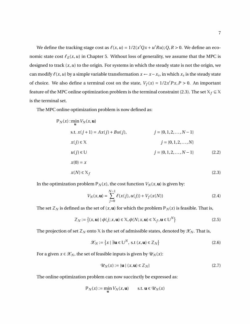


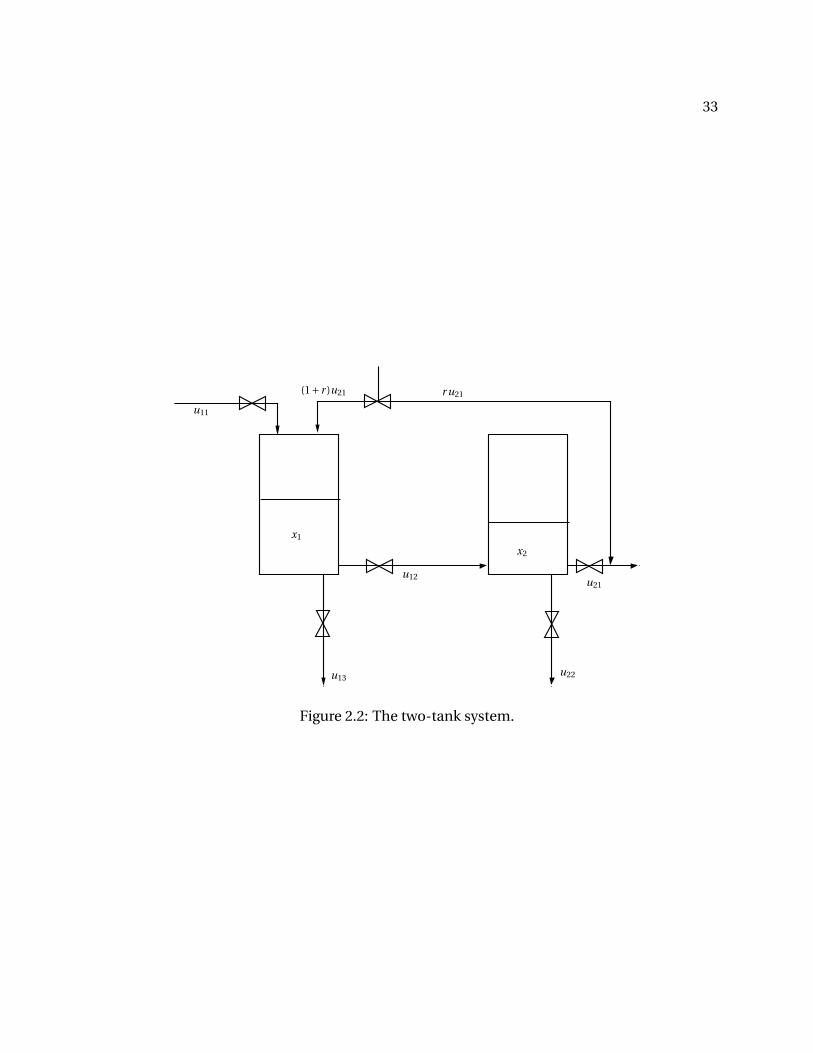
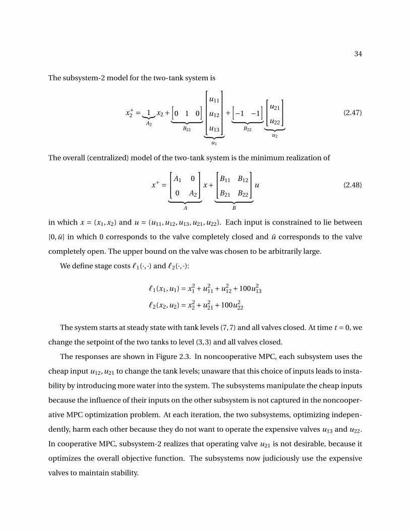
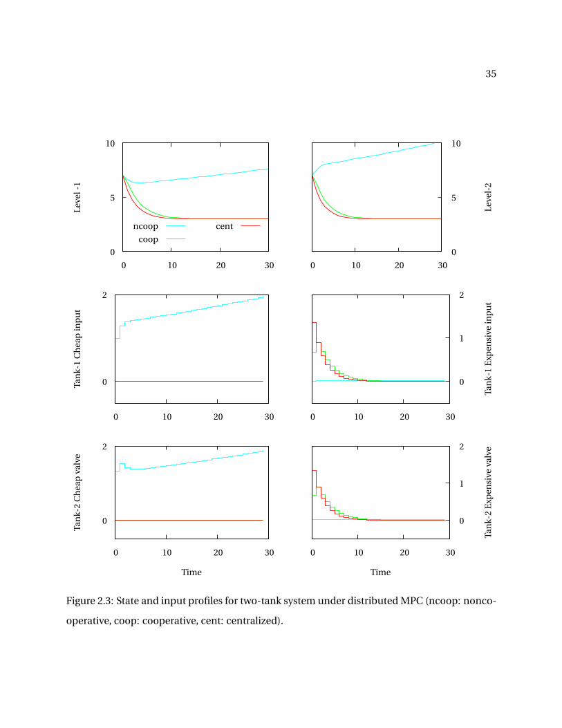


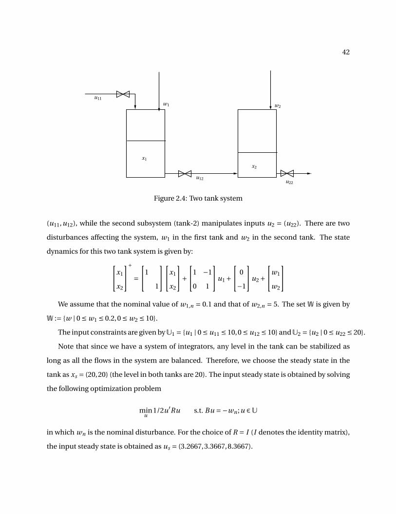
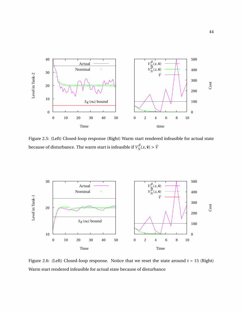


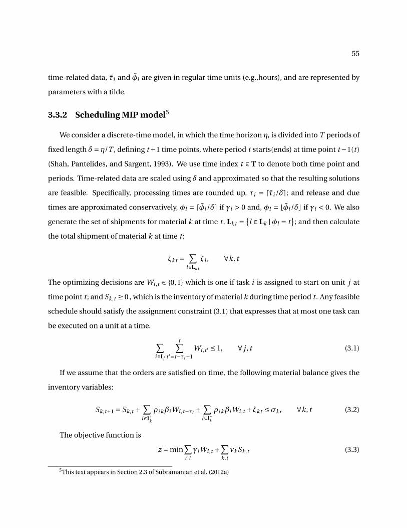
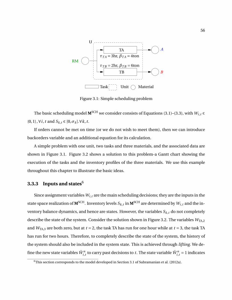


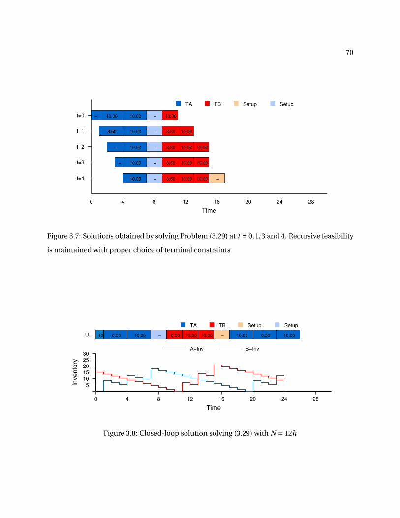
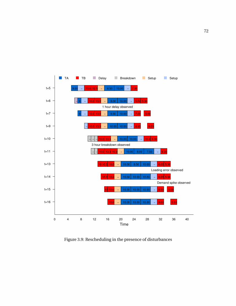
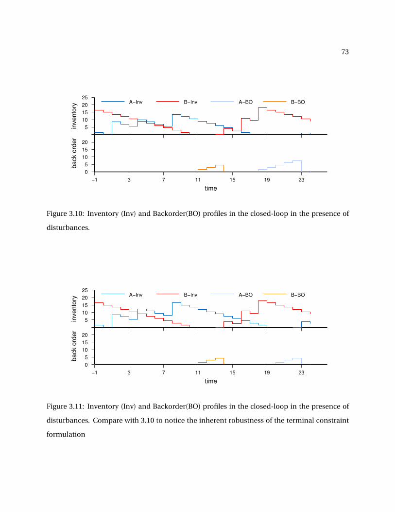


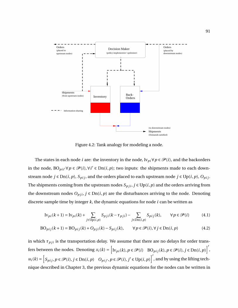


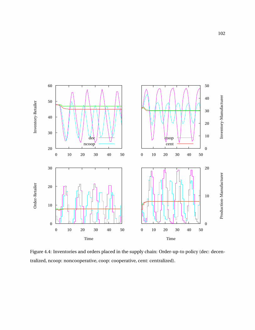
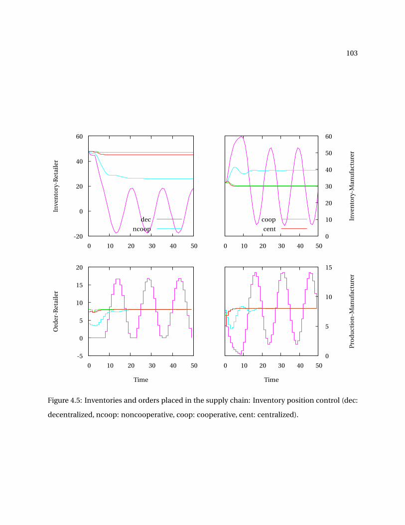
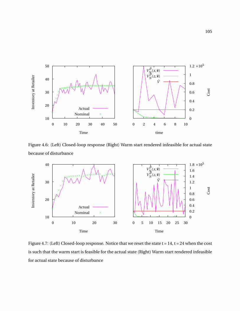

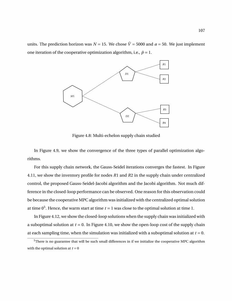
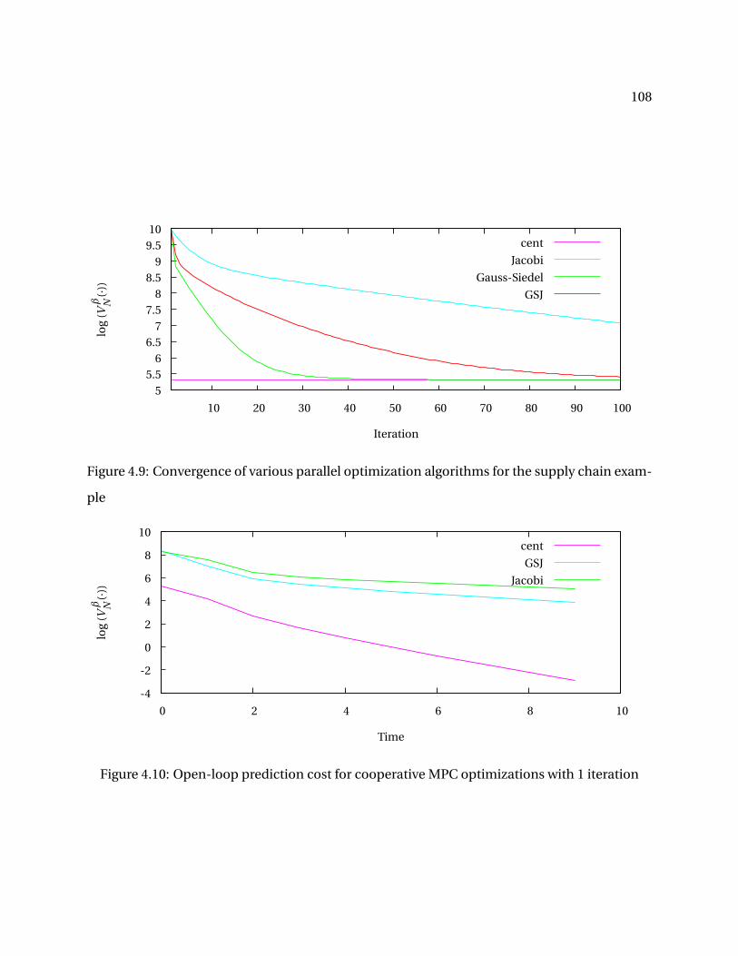
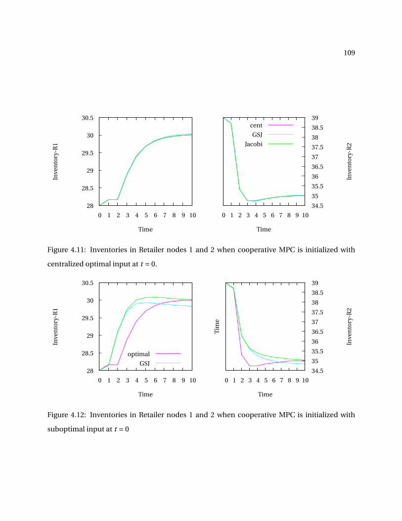
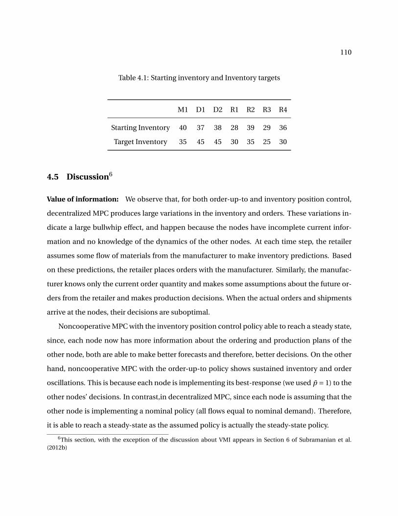


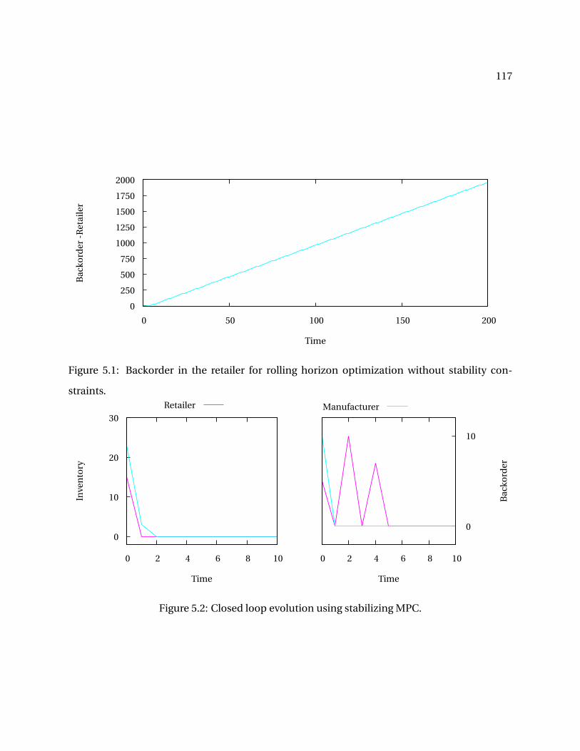


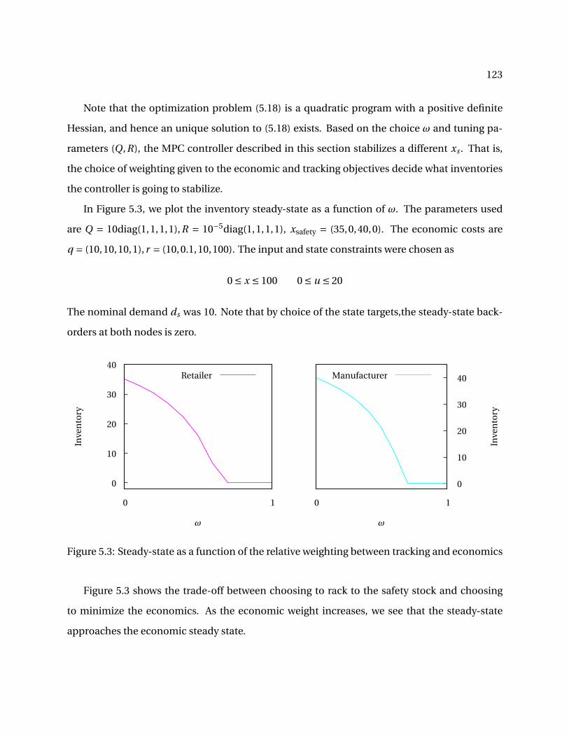
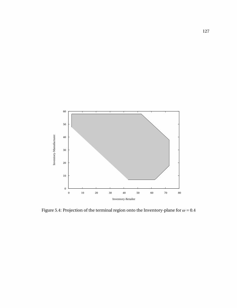

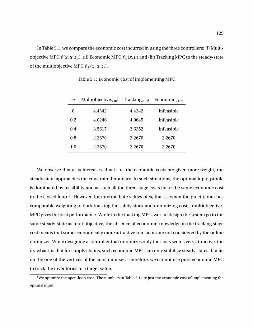


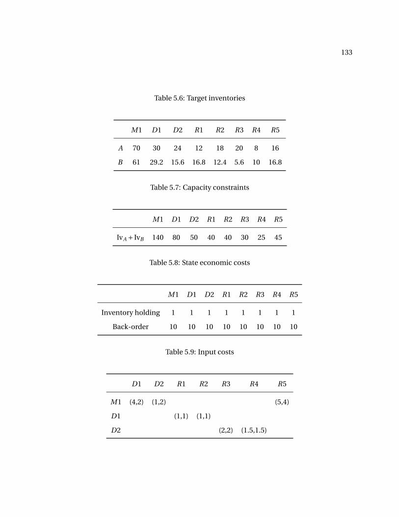
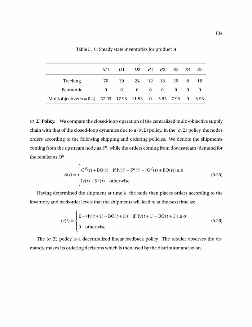
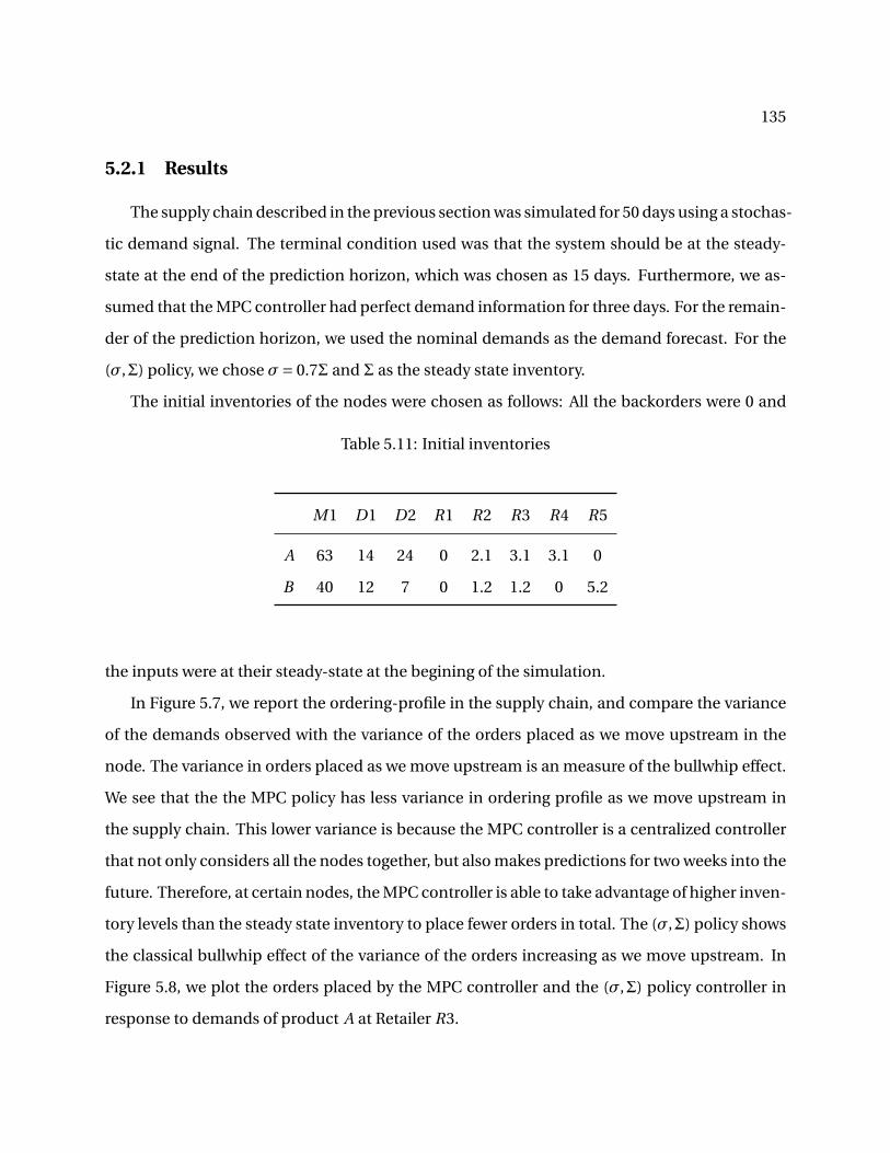
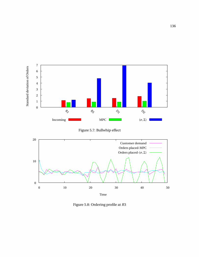
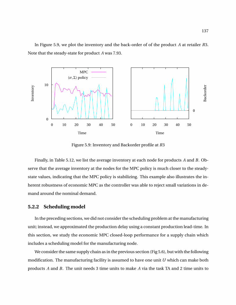
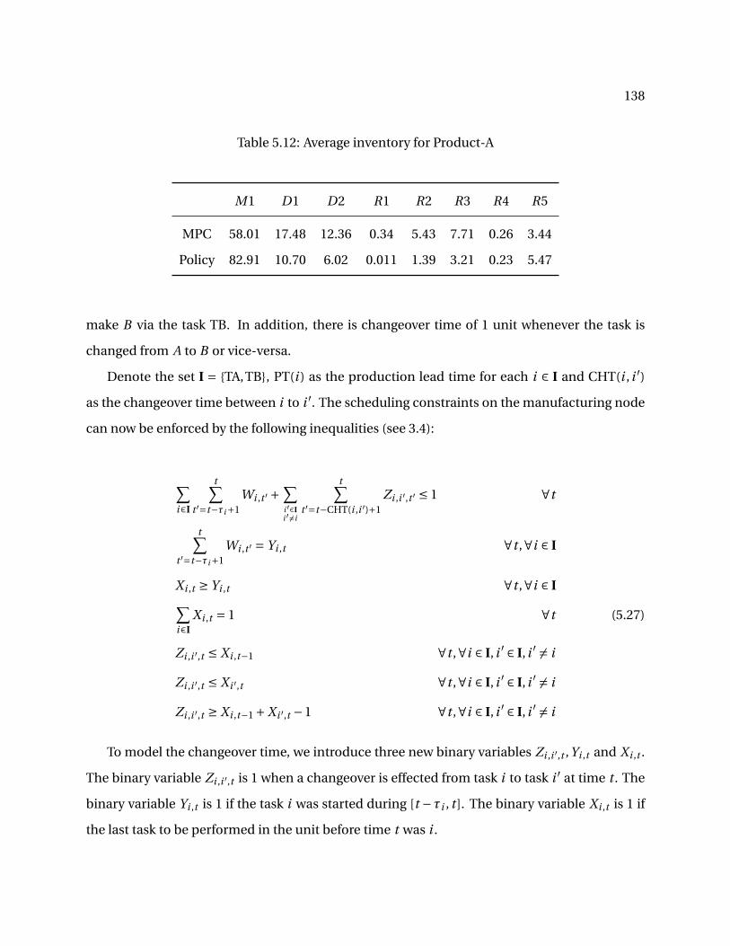
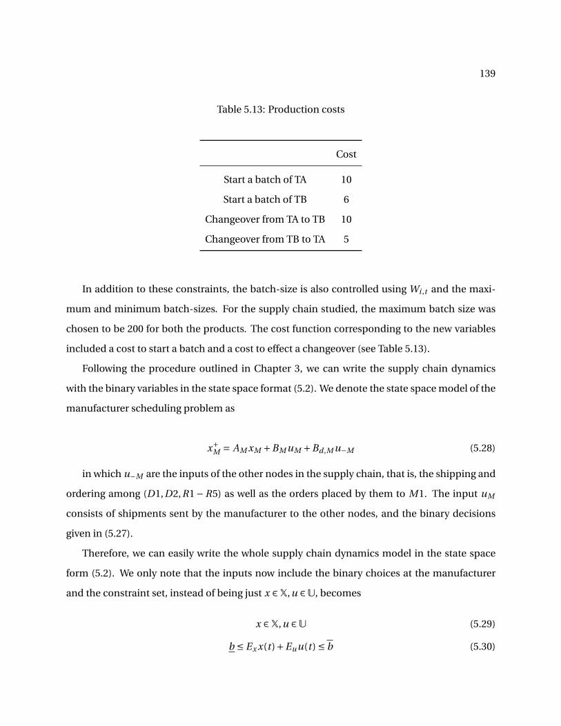
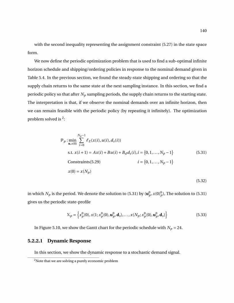
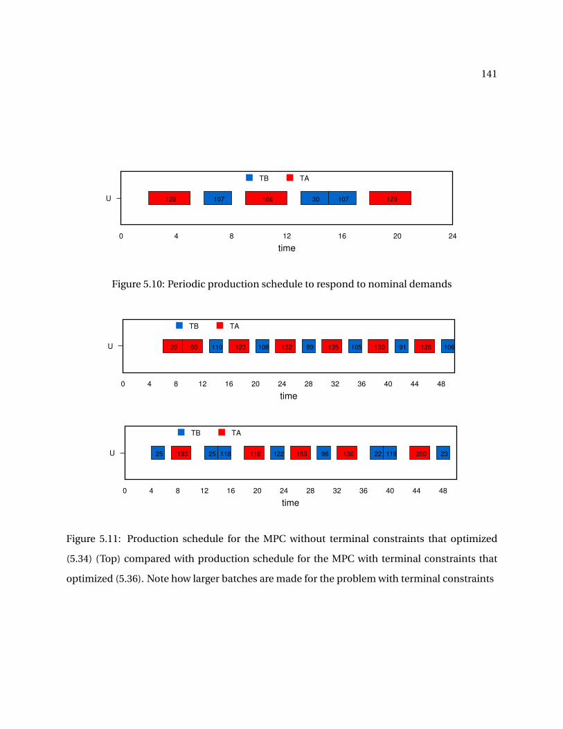


![BP520 JBR 517 JBR - Universal Airlinesuvairlines.com/admin/resources/LHBP.pdfABONY 1L [ABO1L], JBR 1L Licensed to BRITISH AIRWAYS PLC, . Printed from JeppView disc 23-06. Notice: After](https://static.documents.pub/doc/80x56/603a9ab8acfc0749f75c4eb7/bp520-jbr-517-jbr-universal-abony-1l-abo1l-jbr-1l-licensed-to-british-airways.jpg)