Integration of Database Technology and Multibody System Analysis

II

Integration of Database Technology and Multibody System AnalysisClaes Tisell 2000Department of Machine Design, Royal Institute of Technology, S-100 44 Stockholm, Sweden.

Abstract

The design process includes many different activities in which various computationalmechanics tools are used for behaviour modelling of mechanical systems and theirbuilding blocks, e.g. machine elements. These tools usually support large and complexmodels and they produce large quantities of data with a high degree of complexity. Inthese situations, efficient data management and the ability to search and share data areimportant issues to achieve an efficient design process. Today, this ability is usually notsupported by the individual applications even though this probably would improve andfacilitate the ability to search for data on a higher level in the engineering informationsystem.

This work investigates the ability of searching and comparing analysis data withinbehaviour models of technical systems as well as over the analysis results. This is done byinvestigating the potential benefits of integrating modern database technology with amultibody system (MBS) analysis software in the same manner that has been successfullydone for business and administrative applications. This has resulted in an implementedpilot system, named MECHAMOS, that integrates the main-memory resident object-relational database management system (DBMS) AMOS with the symbolic multibodysystem (MBS) software SOPHIA operating in MapleV. This provides MECHAMOSwith both symbolic and numeric mathematical capabilities for MBS analysis and datamanagement capabilities to search and compare engineering data in the database.

The approach, making data managing tools available in a computer aided engineeringsoftware, considerably improves the analysis of technical systems. The analysis is broughtto a higher level through the available query language and the desired data is specified,fairly intuitively, in a query. When the query is processed, the DBMS knows how toretrieve and automatically derive the required data. As shown in some examples, theability to search over stored and derived data in the database is not restricted to a singleMBS-model in MECHAMOS. Because of the implemented materialisation handling, it isalso possible to search, combine, and compare data from several simulation results whichare based on several different models in the database. This extends the ability to performoptimisation from a traditional parameter study to the possibility to analyse and comparedifferent technical concepts through the query language and hereby retrieve thoseconcepts that fulfil certain requirements. If submodel techniques are supported, queriesover a set of components in the database would automatically create, analyse andcompare the possible concepts. This would assist the designer in choosing the bestcomponents for a design.

Keywords : Machine element; Dynamic systems; Multibody System; Kane's Equations ofMotion; Simulation; Submodel; Functional assembly; Object-Oriented;Object-Relational; Database; DBMS; Extensible Query Language;

TRITA-MMK 2000:25 • ISSN 1400-1179 • ISRN/KTH/MMK/R--00/25--SE

III

Acknowledgements

This work has been carried out at Machine Elements, Department of Machine Design,KTH with the main financial funding supported by NUTEK, The Swedish Board forIndustrial and Technical Development.

First, I would like to express my gratitude to my supervisor Professor Sören Anderssonfor all the guidance and support throughout the years. I am also grateful to my co-supervisor, Professor Martin Lesser at the Department of Mechanics, for introducing meand giving me insight in the field of multibody system analysis.

Secondly, I am very grateful to Dr Kjell Orsborn at the Department of InformationScience, Uppsala University, for the guidance and support in the field of databasetechnology.

I would also like to thank all my colleagues at the Department of Machine Design andthe Department of Mechanics for their help and discussions on this subject and manyothers. A special thanks to Dr Anders Lennartsson, a fellow graduate student in thebeginning of my studies, for many clarifying and valuable discussions on MBS analysisand other interesting topics.

Finally, I thank Camilla for support and joyful moments far from technical research andengineering.

Stockholm, October 2000

Claes Tisell

IV

Thesis

This thesis concerns database technology in multibody system analysis and includes thefollowing 6 papers:

Paper A. Tisell, C., Andersson, S., A Functional Interpretation to ConstrainedMotion of Systems, Department of Machine Design, KTH, TRITA-MAE1994:6, ISSN 0282-0048, ISRN/KTH/MAE/R--94/6--SE, 1994

Andersson provided the main ideas of the systems and flow approach and the functionalconcept. Tisell provided the theories of Kane's equations and did all the derivations.Tisell wrote the main part of the paper.

Paper B. Tisell, C., DYMAP - A Dynamic Modular Assembly Package, Proceedingsof the 36th SIMS Simulation Conference, Stockholm, 1994

Paper C. Tisell, C., Orsborn, K., A System for Multibody Analysis Based on Object-Relational Database Technology, Proceedings of the First InternationalConference on Engineering Computational Technology, Edinburgh,Scotland, 18-20 August 1998. In Advances in Engineering ComputationalTechnology, Topping, B.H.V. (ed.), Civil-Comp Press, ISBN 0-948749-55-5, 1998, p. 273-285.

Tisell provided the MBS theories and did the implementation. Orsborn provided thedatabase knowledge. The paper was equally written by the authors.

Paper D. Tisell, C., Computational Efficiency of a Four Bar Mechanism in MapleVand Matlab, Department of Machine Design, KTH, TRITA-MMK 2000:26,ISSN 1400-1179, ISRN/KTH/MMK/R--00/26--SE, 2000.

Paper E. Tisell, C., Orsborn, K., Using an Extensible Object-Oriented QueryLanguage in Multibody Systems Analysis, Proceedings of the SeventhInternational Conference on Civil and Structural Engineering Computing,Oxford, England, 13-15 September 1999. In Developments in Analysis andDesign Using Finite Elements Methods, Topping, B.H.V., Kumar, B. (eds.),Civil-Comp Press, ISBN 0-948749-61-X, 1999, p. 47-54.

Tisell did the implementation and the writing. Orsborn supported the work.

Paper F. Tisell, C., Multibody Systems: Constraint Force Analysis through anExtensible Query Language, Proceedings of the OST-99 conference onMachine Design, Stockholm, 1999.

V

Contents

1. Introduction ...................................................................................................... 1

1.1 Scope and objective ................................................................................... 2

2. Multibody System Analysis .............................................................................. 5

2.1 Multibody system analysis activities ........................................................... 5

2.2 Notation and space organisation ................................................................. 7

2.3 Equations of motion ................................................................................... 8

2.4 MBS software .......................................................................................... 15

2.5 Summary and conclusions ........................................................................ 19

3. Database Technology ...................................................................................... 21

3.1 Databases and database management systems ........................................... 22

3.2 The AMOS object-relational DBMS ........................................................ 25


4. The MECHAMOS Implementation ............................................................... 31

4.1 The MECHAMOS architecture and data comunication ............................ 31

4.2 Base data and derived data ....................................................................... 33

4.3 Using the AMOSQL query language in MBS analysis .............................. 38


5. Summary of Papers ......................................................................................... 45

6. Concluding Remarks ...................................................................................... 49

7. References ....................................................................................................... 53

Appendix 1. Notation and Abbreviations ......................................................... 55

Appendix 2. The SOPHIA MBS-analysis package ........................................... 57

Appended papers:

Paper A. A Functional Interpretation to Constrained Motion of Systems. 61Paper B. DYMAP - A Dynamic Modular Assembly Package. 93Paper C. A System for Multibody Analysis Based on Object-Relational … 105Paper D. Computational Efficiency of a Four Bar Mechanism in MapleV and …133Paper E. Using an Extensible Object-Oriented Query Language in Multibody …147Paper F. Multibody Systems: Constraint Force Analysis through an Extensible …165

1

1. Introduction

Today's complex and high performance products require an efficient productdevelopment process with cutting edge technical knowledge and advanced analysis toolsto be successful in a competitive market. This process includes activities from the ideaand a market opportunity to delivery of the final product. The intermediate activities aretypically the design process, manufacturing, and marketing of the product. An efficientproduct development process results in a shorter time to market and thus lower costs andearlier incomes. The best way to obtain this could be to have activities progress inparallel (or at least with extensive overlapping) and simulation and analysis tools used asearly as possible within the individual activities. This puts requirements on theengineering information system (EIS)1 to be able to search and share heterogeneousproduct information efficiently among the activities.

In the design process, early analyses to predict the behaviour of different concepts hasbecome increasingly important to support the decision making and the choice oftechnical solutions. If the modelling is successful, the physical prototypes--where thedesign parameters are relatively fixed--can validate the technical solutions rather thantrying different solutions. Thus the number of prototypes can be reduced.

To model the behaviour of mechanical systems, advanced computational mechanicssoftware-tools are available such as: computer aided design (CAD) for geometricmodelling; finite element analysis (FEA) for flexible body analyses; computational fluiddynamics (CFD) for flow analyses; and multibody system (MBS) analysis for dynamicanalyses. Between these application domains, data should be shared and reused. CADcould provide the other applications with geometry data, FEA data and CFD data (e.g.pressure and temperature) could be exchanged, and MBS analysis could provide FEAwith dynamic loads and CAD with mechanism motion data for animations. Themodelling capabilities of these computational mechanics tools are improved rapidly withthe hardware development. This enables larger and more complex models as well asimplementation of more advanced analysis methods. In doing so, the software produceslarge amounts of data with a high degree of complexity. Thus, the ability to search fordata within the models as well as over the resulting data becomes increasingly importantin order to perform efficient analyses and to compare different concepts.

Many designs are built up by standard components with well-known properties. Thesecomponents are typically standardised machine elements available from severalmanufacturers. There are also specialised components that fit in several products in amodular product range from a single manufacturer. Thus, it is possible to provide a widevariety of product variants achieved by a relatively small set of product-line-specificmodules of components. The behaviour of these components can be modelled assubmodels where mating features are defined for interaction with other submodels.Modelling is hereby reduced to assembling the submodels to obtain the overall functionaldescription of the design. Again, the ability to search is important, both over the availablesubmodels and over the possible assemblies and their analyses and simulations results.

1 A list of notations and abbreviations are found in Appendix 1.

2

In a multiple user EIS efficient data management and the capability of searching andsharing data is a strategic and critical issue. This capability is important on all levels inthe EIS, from the product development level to the individual analysis tools. It isbelieved that database technology is the key technology to meet these requirements [1].Furthermore, applying database technology on the individual analysis tools will mostlikely facilitate searching and sharing information on a higher level in the EIS. Toaccomplish this object-oriented database technology will probably play an equallyimportant role in engineering applications as relational database technology has done inbusiness and administrative applications.

1.1 Scope and objective

The original objective of this research was to integrate modern MBS methods andformalisms with functional and behaviour modelling of technical systems and machineelements. As mentioned above, functional and behaviour modelling is important in thebeginning of the design process to predict the dynamic behaviour of the technical systembeing designed. The functional goal of the system is usually formulated in a specificationat an early stage. As a physical product is more or less an assembly of machine elements,this goal can usually be achieved by several different technical solutions which differ inthe choice of machine elements. With MBS models representing the function andbehaviour of the system, the different possible solutions could, at an early stage, beanalysed and compared by simulations to support the final decision of the most suitabletechnical concept. In these situations, submodel techniques can be used to reduce themodelling effort to assemble pre-defined modules that represents the functionalbehaviour of the components. Submodel techniques are thus an assisting tool to thedesigner in choosing machine elements for a design. At a later stage in the designprocess, when the main functional concept is chosen, or at least the number of conceptsis narrowed down, functional and behaviour modelling is still important. It can now beused to optimise and investigate the robustness of the design, by analysing somefunctional response for various design parameter values.

In the appended paper A, a general structure for functional modelling of machineelements is discussed. The modelling is based on a systems and flow approach where thetechnical system is divided into subsystems and energy flows through and between thesystems are formulated. The approach is related to MBS methods for deriving equationsof motion. In paper B, these ideas are implemented in a computer algebra system. In thisimplementation pre-defined submodels, for which the energy flows are formulatedsymbolically, are stored in a library. These submodels are then assembled in the software,the equations reduced due to the imposed constraints on the submodels and theequations of motion obtained on symbolic form.

As the work evolved, it was found that the way basic data and submodels are stored isimportant for the ability to perform the analyses. For instance, data managing toolsprovided by database technology will most likely improve the ability to search forcomponents, models, simulation results etc. Due to this insight, the original objectivewas refined for the second part of the thesis to focus on the potential benefits ofintegrating modern database technology with MBS analysis software. The goal with thisapproach is to implement as much knowledge and basic data into the database as

3

required, enabling the database management system (DBMS) to perform the analysesand search over the data. In the field of MBS analysis, this puts requirements on theDBMS to a) provide suitable data types for MBS-data, b) derive ordinary differentialequations that describe the motion of the mechanical system and c) solve these non-linearequations using numerical methods.

This approach, building computational mechanics applications based on modern databasetechnology, is investigated primarily by implementing a research prototype software forMBS analysis named MECHAMOS. The MECHAMOS system integrates the main-memory resident object-relational DBMS AMOS [2,18] with the symbolic MBSsoftware SOPHIA [3]. This integration is enabled by extending the AMOS DBMS withthe computer algebra system MapleV [19,20] for symbolic manipulation and Matlab [21]for numeric manipulation. The MECHAMOS system is hereby provided with datamanagement capabilities from AMOS and MBS analysis capabilities from SOPHIAthrough MapleV and Matlab.

The objective with the MECHAMOS system is to show if and how advanced analysescan be performed in a database environment. No effort has been put on graphical anduser friendly interfaces as it is not claimed to be a ready-to-use MBS software.Furthermore, the intention has been to support analysis of certain classes of problems byimplementing general database functions that enables database queries to search for dataderived by the DBMS. In papers C to F, the implementation and work related toMECHAMOS is presented and discussed.

In the remainder of this thesis introduction, the next chapter discusses multibody systemanalysis in a general manner where different methods for deriving the equations ofmotion as well as various MBS software strategies are discussed. In chapter 3 databasesystems are discussed and in chapter 4 the MECHAMOS system is presented with someexamples showing the benefits of a query language in simulation of mechanical systems.

4

5

2. Multibody System Analysis

Multibody system (MBS) analysis is important in the design process as it is a tool todetermine the motion of mechanical systems. One of the prime objectives with thisanalysis is to determine forces and loads acting in the system. These forces are typicallyspring forces, reaction forces in bearings and fixed joints etc.

The purpose of this chapter is to give an introduction to MBS analysis. It starts with adescription of multibody systems and the MBS analysis process. An important phase inthis process is the actual derivation of the equations of motion. Four different methodsfor deriving these equations are described: the Newton-Euler equations, Lagrange’sequations, Kane’s equations, and the systems and flow approach. Furthermore, MBSanalysis software is discussed with advantages and drawbacks pointed out for thedifferent software categories. Finally, the ideas behind and the working procedure in theSOPHIA software for MBS analysis are described. In Appendix 2, the most importantSOPHIA commands are presented and a SOPHIA file that derives the equations for asliding pendulum configuration is also appended. Related appended papers to thischapter are:

• paper A which shows the close relation between the flow approach and Kane’smethod in deriving the equations of motion. The systems approach is discussedfrom a machine element point of view resulting in submodel techniques.

• paper B which presents a pilot software for MBS analysis based on the systemsand flow approach presented in paper A. The software assembles pre-definedsubmodels and automatically derives the equations of motion for these assemblies.

• paper D which studies the CPU time to derive symbolic equations of motion ondifferent forms and further numerically evaluate these equations.

• paper F where the projection approach of Kane’s method and constraint forceanalysis are thoroughly discussed.

2.1 Multibody system analysis activities

A multibody system is a mechanical system composed of bodies that are influenced byforces and moments. These bodies are interconnected to each other by different types ofjoints that constrain the relative motion of the bodies in different directions. To facilitatethe description of the system, the bodies are considered to be rigid. This implies that onlysix coordinates are needed to fully describe the state of an unconstrained body (threetranslational coordinates for the position of the centre of mass and three rotationalcoordinates to determine the orientation). These coordinates are functions of time andthe primary task in MBS analysis is to determine how they vary in time. The rigid bodyassumption also implies that flexibility of a mechanical system is modelled as appliedforces on the surrounding bodies and is normally represented by massless springs. Thisassumption is valid if the flexibility of the bodies or the masses of the springs do notconsiderably influence the dynamic response of the mechanical system.

6

The MBS analysis can be divided into different phases as illustrated in Figure 1. In Phase1 of the analysis, the physical system is described in terms of a mathematical model. Thismodel defines the objects, the degrees of freedom of the system in terms of coordinatesand coordinate systems, and the forces and moments acting on the individual bodies.

Phase 2 of the analysis is to derive the equations of motion that, in some sense, describesthe behaviour of the system. There are various methods available to the analyst toaccomplish this and it can be done in a fairly systematic fashion. Some of the methods arebriefly described below. The resulting equations are usually 2nd order non-linear ordinarydifferential equations (ODEs) with time as the integration variable.

Because of the non-linearities in the resulting equations, the analysis moves from thesymbolic domain to the numeric domain in Phase 3. In this phase, the equations areintegrated numerically, starting from a set of initial values of the coordinates and theirtime derivatives (i.e. state variables). The result of Phase 3 is numeric values of the statevariables for each time step of the integration (i.e. the trajectories of the equations).

With the state variables numerically known, kinematic and dynamic information (e.g.accelerations, energies, reaction forces etc.) can be derived on symbolic form (Phase 4a),evaluated numerically (Phase 4b), and interpreted in Phase 4c. This interpretation istraditionally done by visual inspection and comparison of the data which usually isrepresented as plots and animations.

In addition to integrating the ODEs, a qualitative analysis of the equations (i.e.equations of motion) can provide important information about the mechanical system(Phase 5). Such an analysis includes finding critical points, linearising the equationsaround these points, and determining the stability of the system at these critical points.This, however, is not further discussed in this thesis.

Figure 1 Different domains and different phases in multibody system analysis.

7

2.2 Notation and space organisation

The description of the mathematical model in Phase 1 requires a strict and logicalnotation. This thesis basically adopts the notation introduced by Lesser [4,5] in which thesystem vector is an important object. To define this object, consider a multibody systemof k rigid bodies with a total of n degrees of freedom. Assume, for now, that the systemis not subjected to additional holonomic or nonholonomic constraints. The system isdescribed by n generalised coordinates (q) and there are reference frames (fA) rigidlyattached to each of the bodies in the system. These frames are defined relative to someinertial frame (fN) by some of the generalised coordinates. The position vector (r),velocity vector (v) and angular velocity vector (ω) can now be formulated for each of thebodies. To organise the entire MBS in one object, Lesser introduced the system vector2

that gathers information of all the bodies in the system. The system velocity vector (v<) istypically

[ ]v v v< < < < <= 1 1ω ω�

k k T(1)

Thus, the system vector is a column vector denoted by the superscript (<) and contains ofone vector with translational- (v) and one vector with rotational information (ω) for eachof the k bodies in the system. Analogously, the system force vector contains force andmoment vectors. The introduction of the system vector calls for a definition of anadditional operator, the fat dot product, to obtain the component wise scalar product oftwo system vectors If A<i is the i:th vector in the system vector A<, the fat dot product isdefined as

A B A B< < < <

=• = ⋅∑ i i

i

k

1

(2)

Geometrical interpretations of MBSs have enhanced the understanding of the differentmethods of deriving the equations of motion. In this interpretation, an unconstrainedconfiguration space of dimension 6k is considered. This space is defined by the numberof bodies in the MBS and is spanned by two subspaces, the tangent space (of dimensionn) and the complementary space (of dimension 6k-n). The motion of the system takesplace in the tangent space and the directions in which the MBS is constrained span thecomplementary space.

With the geometrical interpretation and its two subspaces, the forces acting on theindividual bodies can be divided into two categories, applied forces and constraintforces. Applied forces are usually known in terms of the position and velocity (i.e.spring, damping, friction, and gravity forces) and they exist mainly in the tangent space.The constraint forces keep the bodies on a constrained path (i.e. normal force) and areusually functions of the accelerations. These forces only exist in the complementaryspace.

2 Lesser calls this a K-vector referring to the k bodies in the MBS. In SOPHIA this data type is referredto as a KM-vector.

8

2.3 Equations of motion

A central part in MBS analysis is the actual forming of the equations of motion. Thevarious methods available for this are all based on the three fundamental laws stated byIsaac Newton (1642-1727) back in 1687 [6]:

I Every body continues in its state of rest or uniform rectilinear motion,except if it is compelled by forces acting on it to change that state.

II The change of motion is proportional to the applied force and takesplace in the direction of the straight line along which that force acts.

III To every action there is always an equal and contrary reaction; or, themutual actions of any two bodies are always equal and oppositelydirected along the same line.

The desire when formulating the equations of motion is to obtain the equations in anefficient way and then put these equations on a suitable form that is efficient for furthernumeric evaluation. Some methods aim for a minimal set of constraint reaction freeequations of motion whereas others formulates more equations to determine not only thecoordinates but also the constraint forces appearing in the equations. The former groupof methods results in n ordinary differential equations (ODEs) and the latter results in amaximum of 6k differential-algebraic equations (DAEs).

The equations discussed here are valid when the relativistic and the quantum effects aresmall, i.e. velocities much smaller than the speed of light and actions are much largerthan Planck’s constant respectively, [7].

The Newton-Euler equations of motion

Assuming that "body" in Newton's laws above is an idealised mass, m, with no spatialextension (a particle), the second law may be written as

F a= m (3)

where the vector F is the sum of all forces, including constraint- and applied forces, onthe body. The change of motion, a, is the acceleration vector and the proportionalconstant, m, is the mass. Equation (3) describes the translational motion of the body. Forrigid bodies (they have spatial extension) a second equation is required to determine theorientation, this to fully describe the state of the body. Euler (1707-1783) formulated thisequation for the rotational motion of rigid bodies as

M J h= ⋅ + ×�ω ω (4)

where ω is the angular velocity vector, J is the moments of inertia dyad, and M is themoment vector around the centre of mass. Introducing the linear and angular momentum

p v= m and h J= ⋅ωω (5)

respectively, where v is the velocity of the centre of mass, the Newton-Euler equationsof motion for prediction of dynamic systems are

9

F p= � and M h= � (6)

In the system vector notation, described above, and with applied (R a< ) and constraint

( R c< ) forces separated, the Newton-Euler equations (6) for an MBS can be rewritten as

R R pa c< < <+ = � (7)

These equations yields, in the general case, a set of 6k (3k in a planar case) DAEs fordetermining the n coordinates and the 6k-n constraint forces and constraint moments.

Lagrange’s equations

The Newton-Euler equations are widely used and known by many engineers. As acomplement to Newton-Euler, Lagrange (1736-1813) presented an alternative method toformulate the equations of motion in the end of the eighteenth century. Rather than for-mulating the momentum and forces as in Newton-Euler's method, this method is basedon formulating the kinetic and potential energy for the system in terms of the introducedgeneralised coordinates (q). The 1st and 2nd form of Lagrange’s equations are then

d

dt q qK Q

j jj

∂∂

∂∂�

−

= and

d

dt q qL

j j

∂∂

∂∂�

−

= 0 (8)

where the Lagrangian L = K - V is the difference between kinetic (K) and potential (V)energy in the system. The generalised force (Qj) is the force or moment component in thedirection of the generalised coordinate qj. Lagrange’s equations result in a minimal set ofn constraint reaction free second order ODEs for determining the n generalisedcoordinates.

Kane’s equations

In the 1960’s, Kane presented a alternative method for MBS analysis [8], also resultingin a minimal set of constraint reaction free equations in the same manner as Lagrange’sequations. This method, or equations, was later given a geometrical interpretation byLesser, [4]. According to Lesser, Kane’s equations are ”projections of the Newton-Euler’s equations of motion onto a spanning set of the configuration manifold’s tangentspace”. This tangent space is essentially spanned by the instantaneous possible directionsof motion of the system. Figure 2 illustrates this for a particle constrained to move on asphere where β j

< (j = 1 , ... , n) are the n tangent vectors that span the n dimensional

tangent space. With Lesser's interpretation, Kane's equations are obtained by projectingEquation (7) onto the tangent space (β j

< ). In system vector notation, Kane’s equations

are

R pa j j< < < <• = •β β� (9)

10

The term including the constraint forces vanishes since the tangent space is orthogonal tothe complementary space in which the constraint forces exist. This can also be statedbased on an interpretation of D’Alembert’s principle which says that the work done bythe constraint forces during a displacement compatible with the constraints is zero, [9].This orthogonality between the constraint forces and the tangent vectors is, in systemvector notation, formulated as

R c j< <• =β 0 (10)

Figure 2 A particle constrained to move on a sphere illustrating the tangent vectors that spanthe two-dimensional tangent space embedded in the three-dimensional configuration space.

Kane also introduced the concept of generalised speeds (u). These generalised speedsare chosen, by inspection, as arbitrary linear functions of the generalised velocities (�q ).The relation between the �q and u is called the kinematic differential equations (kdes) andare thus

( )� ,q f u qj j= (11)

Each time a differentiation with respect to time is performed these kdes have to besubstituted into the result. Hereby, the motion of the system is represented by a set oflinearly independent generalised speeds. The set of tangent vectors, β j

< , that span the

tangent space is now found from the system velocity vector (v<) as

β jju

<<

=∂∂v

(12)

All the terms in Kane's equations3 (9) are now defined and notable is that there are noextra information required in Kane's method compared to other methods. The tangentvectors are easily computed with Equation (12) and the kdes are defined prior to theformulation of the equations of motion rather than prior to the numerical integration, asis the case in other methods. The resulting equations of motion are a) the n equations 3 The components of the tangent vectors are named partial velocities by Kane. Kane has also introducedthe generalised active force (Fj) and the generalised inertia force (Fj

*). They are defined as the left handside and the right hand side of Equation (9) respectively.

11

obtained from Equation (9) (one equation for each independent tangent vector) and b)the n kdes of Equation (11). Thus, by the introduction of the generalised speeds, thismethod yields a set of 2n constraint reaction free first order ODEs ready for numericintegration.

Kane’s and Lagrange’s equations

Kane’s equations (9) are directly related to Lagrange’s equations (8a), or vice versa, ifthe generalised speeds of Equation (11) are defined on the simplest form, i.e. u qj j= � .

This close relationship is then [5]

d

dt q qK

j jj

∂∂

∂∂�

�−

= •< <p β and Qj a j= •< <R β (13)

A difference between the two methods is the effort required deriving the symbolicequations, which is in favour for Kane’s method. Furthermore, the intuitiveunderstanding of how and why the constraint forces automatically vanish from theequations is enhanced with Lesser’s geometrical interpretation of Kane’s equations.

Kane’s equations and constraint forces

Kane’s equations usually determine the motion of the mechanical system without havingto solve for the constraint forces. However, determining the size and direction of one orseveral constraint forces may also be one of the objectives of the MBS analysis. This iseven necessary to be able to determine the motion if the applied forces are dependent onthe constraint forces (e.g. dry friction). To determine the constraint forces in Kane’smethod, the Newton-Euler equations (7) are projected onto the complementary spacerather than the tangent space, thus

( )R R pa c i i< < < < <+ • = •γ γ� (14)

where γ i< are the vectors that span the complementary space. It is in this space that the

constraint forces exist and the constraint forces can thus be expressed as a linear combi-nation of the γ i

< -vectors. The issue of constraint force analysis with Kane’s method insystem vector notation is discussed in the appended paper F. One of the results from thisdiscussion is that, for a proper choice of the γ i

< -vectors, it is possible to obtain a set ofequations that are uncoupled in the constraint forces (i.e. each equation contains onlyone unknown constraint force). The γ i

< -vectors required to achieve this are defined bythe fictitious coordinates (qf) introduced in the directions of the constraint forces. Fromthese fictitious coordinates, the fictitious system velocity vector (v f

< ) can be derived and

hereby, in the same manner as the tangent vectors, the γ i< -vectors are derived by

γ i

f

fiq<

<

=∂∂v

�

(15)

12

In the example of Figure 2, the complementary space is one-dimensional and is in thenormal direction to the sphere. Projecting the Newton-Euler equations (7) onto thatdirection yields an additional equation that determines the force constraining the particleto remain on the sphere.

The contribution of paper F in the field of MBS analysis is the geometrical interpretationof Kane’s constraint force analysis in terms of Lesser’s system vector notation. Further,the paper points out how these γ i

< -vectors are found in a systematic fashion. The

benefits of this method are that we only have to keep track of which γ i< -vector

corresponds to which constraint force in order to determine a specific constraint force.Traditionally, an equation is formed for the constraint force. Depending on how manyunknown constraint forces this equation contains, additional equation have to be formeduntil the constraint force in question can be solved for. The method presented in paper Fseems to be well suited for computer implementation and is used in MECHAMOS todetermine the constraint forces.

Systems and flow approach

In engineering design and machine elements, products are often considered as technicalsystems. A technical system is a set of functional elements interrelated to each other andto the whole such that a common goal is achieved. The behaviour of the technical systemis dependent on the technical process in which energy, material and/or signals arechannelled and/or converted [10]. In the systems approach [11], used in this thesis, acontrol volume is defined that encloses the system to be analysed and separates thesystem from the environment. Interaction between the system and the environment isassumed to take place through discrete regions that are named ports. A system in it selfcan be further divided into subsystems with additional ports defined for interactionbetween the subsystems. This systematic approach usually enhances the understanding ofthe physical system and facilitates the modelling procedure.

The next step is to analyse the system using the flow approach [11] where material,signal, and energy flows through and in the control volume are studied. In mechanicalsystems the control volume may be defined such that the material and signal flows can beneglected. Thus, left to be analysed is the energy flow. Energy can not be created ordestroyed, but it is transformed between various energy domains (e.g. mechanical,electrical, thermal). Therefore the energy flows through the system, due to conservationof energy, can be formulated as

( )Pt

W Pin out stored transf− − + =dd

0 (16)

This is basically an interpretation of the first law of thermodynamics where Pin-out is thenet energy flow into the system through all defined ports, Wstored is the energy stored inthe system, and Ptransf is the energy transformed between various domains. Each energydomain may be looked upon separately and Equation (16) applied on the mechanical andthermal domain consequently results in the following two equations:

13

( )Pt

W Pin outmec

storedmec

transfmec

− − + =dd

0 (17)

( )Pt

W Pin outtherm

storedtherm

transftherm

− − + =dd

0 (18)

The last term in Equation (16), Ptransf , is the energy flow transformed within the system.Again, energy can not be created nor destroyed, therefore the sum of all transformationsin the system, Ptransf , is zero. However, communication between the various energydomains takes place through this transformation term and each transformation containsone term of each energy domain involved in the transformation (a sink-source pair).Typically, losses in mechanical systems are energy transforming from mechanical tothermal energy, e.g. friction or damping. The energy is then leaving the mechanicaldomain (negative) and entering the thermal domain (positive). Thus the transformationterm will then take the form

P P Ptransf transfmec

transftherm= + = 0 (19)

These ideas, using the systems and flow approach in the analysis of mechanical systems,are discussed in paper A. One part of this discussion focuses on how the equations ofmotion are obtained from the formulated energy flows according to equation (17). Theenergy flow, or power (P), is the product of an effort and a flow variable which both canbe represented by vectors. In the mechanical domain, the effort and flow variables areforce and velocity for the translational part and moment and angular velocity for therotational part. This implies that the power is a projection of the forces onto thevelocities. As the tangent space in Kane's method is found from the velocity vectors,these two methods are closely related and the equations of motion is found from

∂∂u

PtW P

jin outmec

storedmec

transfmec

∗ − − +

=

d

d0 (20)

where u* are the generalised speeds that origin from the velocities in the powerexpressions. The difference between the methods is that the velocity vector isdifferentiated with respect to the generalised speeds prior to formulating the equations ofmotion (to obtain the tangent vectors) in Kane’s method. In the energy approach this isdone after the energy flows have been formulated. The resulting equations are a set of 2nfirst order ODEs found from: a) the n equations obtained from Equation (20) and b) then kdes of Equation (11).

A functional interpretation of the terms in Equation (17) is also discussed in paper A.The different terms (and combinations of) are associated with the four basic functionsthat a subsystem can posses [11]. These basic functions are to store something,transform something, transport something, and support something.

Holonomic and nonholonomic constraints

In the above sections it was assumed that a set of independent generalised coordinateswere used to describe the MBS. If redundant coordinates are used (i.e. more coordinates

14

that degrees of freedom), additional constraint equations have to be formulated to relatethe redundant coordinates to the independent coordinates. These geometrical constraints,called holonomic constraints, are for example useful in the description of closed loopmechanisms. Holonomic constraints can be written on the form

( )f q qindep holo1 0, = (21)

Differentiating these equations once with respect to time (utilising the concept of kdesdefined in equation (11)) yields equations that constrains the corresponding generalisedspeeds:

( )f u u qindep holo2 0, , = (22)

Another type of additional constraints is the nonholonomic constraints. They are a set ofconstraint equations among the velocities that cannot be integrated to obtain a set ofgeometric constraints. A typical example is rolling without sliding where the two bodiesin contact must have the same velocity in the point of contact. This condition yields anequation relating the involved generalised speeds and the nonholonomic constraint can bewritten on the form

( )f u u qindep nonholo3 0, , = (23)

Both types of constraints are now expressed in the same form and can thus be treated inthe same way. Solving Equations (22) and (23) for the dependent generalised speedsyields

( )u f u qholo indep= 4 , (24)

( )u f u qnonholo indep= 5 , (25)

An example of formulating Equations (21-25) are found in paper C where the providedMBS example is subjected to holonomic and nonholonomic constraints.

The additional constraints of Equations (24) and (25) are treated differently in differentmethods. In the Newton-Euler method, the kdes of equation (11), Equation (7), andEquations (22) and (23) differentiated a second time are forming the set of equations thatdescribes the system. When solving these equations, the initial conditions of thedependent q and u must all fulfil the constraint equations (21-23).

In methods that aim for a minimal set of equations in a minimal set of generalised speedsby projecting expressions onto the tangent space, it is crucial that this tangent spacerepresents the fully constrained system (i.e. the actual motion of the system). To obtainthis for Kane’s method, the system velocity vector in Equation (12) must include all thevelocity constraints imposed on the system. Thus, it is vital that Equations (24) and (25)are substituted into the system velocity vector prior to deriving the tangent space withEquation (12). The same applies to the flow approach where the u* of Equation (20)must be linearly independent and thus the velocities used in the power expressions mustrepresent the actual motion of the system.

15

In the resulting equations of these two methods, the dependent generalised speeds aresubstituted with Equations (24) and (25). The initial values of the holonomic constrainedcoordinates (the dependent q) must then fulfil Equation (21) whereas the unconstrainedcoordinates (the independent q) and the generalised speeds (u) can be chosen arbitrarily.

2.4 MBS software

MBS analysis assistance is offered by many different software packages and they can bedivided into two categories [12,13]. The first category operates entirely in the numericdomain and the software derives the equations of the present mechanism prior to eachanalysis. In this category we find widely used commercial software packages likeADAMS and DADS. The second category first derives the equations in the symbolicdomain and then moves to the numeric domain for solving the equations. Hereby thesymbolic equations are available and can be reused in various analyses that only differ inthe parameter and initial values. In this category we find software packages likeNEWEUL, SD/FAST, AUTOSIM, SIMPACK, SOPHIA, AUTOLEV.

The transition of the equations from the symbolic to the numeric domain in the secondcategory software is usually done automatically by exporting the equations as ready-to-compile C or FORTRAN files. The software either produces a) a numeric simulationprogram, b) subroutines that can be merged into a simulation program, or c) a filecontaining the equations suitable for an existing simulation program. The existence ofsymbolic equations offers flexibility in manipulating the equations prior to the transition.It is for instance, possible to do operations on the equations once in the symbolic domainwhereas in the numeric domain the same operation might have to be performed possibleseveral times at each time step of the integration. Hence, optimisation techniques in thesymbolic domain can be used to put the equations in a computational efficient form forfurther numeric evaluation. This can be done by finding common subexpressions in theequations and substitute these with intermediate variables [14] (e.g. in SOPHIA andAUTOLEV). The subexpressions are then computed once in the beginning of thenumeric evaluation and the result is repeatedly used in the equations. Thus, the numberof arithmetic operations needed to compute the derivatives of the state variables arereduced and the numeric efficiency is improved. Some software also allows specificdefinition of angles known to be small (e.g. AUTOSIM) enabling automatic linearisationof the equations with respect to these small angles [13].

Advantages with the symbolic formulation of the equations of motion are a) theflexibility of parameterised equations, b) that the equations can be put into acomputational efficient form and c) the very fast numeric evaluation through thecompiled C or FORTRAN programs. A drawback with the symbolic formulation is thatthe size of the equations grows rapidly with the degrees of freedom in the system. Theprocess of transforming vectors back and forth between reference frames increases thenumber of operations to obtain the resulting equations. This can be reduced by utilisingdelayed component evaluation techniques [14]. Operations that require transformationsare not performed until it is absolutely necessary and expressions like a1·b1 are thus keptas long as possible. The number of terms in numeric equations are also less than in thecorresponding symbolic equations. For instance, the two symbolic terms m q m q1 1 2 1�� + arereduced to a single term with m1 and m2 numerically fixed as in the numeric equations.

16

Modelling and analysis in MBS software

Some of the MBS software provides a graphical interface to interactively define themechanism (Phase 1 in Figure 1). The different bodies are then created in 3D andinterconnected by predefined joints. Usually these software also offer the possibility toimport the mechanism geometry from an external geometric modeller, e.g. CAD system.However, this import of data is not always successful and may require some furthermodelling and adjustments in the MBS software but it is a valuable assistance of reusingexisting data from another data source. Another approach is to build the MBS-model bya sequence of software specific commands. This can be done either interactively or byreading a text file that contains the sequence of commands. This approach is used in theSOPHIA system and is described in more detail below.

After the mechanism has been defined, the equations of motion can be derived (Phase 2)and further integrated (Phase 3). Depending on which method that is used for derivingthe equations, the results are the state space variables (the generalised coordinates andthe generalised speeds) or, as in ADAMS for instance, six coordinates for each body (thethree translational coordinates for the centre of mass and the three rotationalcoordinates). The results are then presented as graphs or as animations (Phase 4).Animations are used to view the motion of the mechanism graphically and this is apowerful tool for verification of the MBS-model. Inconsistencies in the model can forinstance be detected if connected bodies are separated during the simulation. Thereasonableness of the mechanisms overall motion and the initial conditions are also easilyverified by an animation.

Plotting various properties provides a more accurate view of the simulation results. Thisincludes plotting coordinates and expressions of these such as velocities and constraintforces. In the numeric category of software, plotting the velocity of a point in a body canonly be done automatically for points defined prior to the solving of the equations. For apoint not predefined, due to the lack of symbolic capabilities, the user have to manuallyderive an expression of that velocity in terms of the coordinates and type in theexpression in terms of the variable names for the coordinates to enable numericevaluation.

In the second category of software, moving from the symbolic domain to a separatesimulation program in the numeric domain, symbolic knowledge about the MBS isusually lost. Positions, velocities etc. derived in the symbolic domain to obtain theequations of motion are not available in the numeric domain where the only MBS-dataare the state space variables and how they vary in time. Thus, for the above velocityexample, even in this category, the expression has to be typed in for numeric evaluation.If the symbolic domain is available in the numeric analysis (as in MECHAMOS), newsymbolic expressions combined with existing symbolic expressions (e.g. angularvelocities and velocities of the centre of mass) will assist the user in deriving the desiredvelocity expression and further evaluate this expression numerically.

Further, it is usually support in the software for other numerical analysis results than justthe coordinates from the simulation. The selection of the resulting MBS-data is howevertraditionally done by visually inspecting plots. There is little or no support for efficientMBS-data management resulting in a poor ability to search for MBS-data and no support

17

for analysis and comparison of several MBS-models. To handle these issues in thetraditional MBS software, extensive programming efforts are required of the user andthis usually results in MBS-model and analysis specific programs.

The SOPHIA system

Development of a new symbolic based MBS software can either be done from scratch orbe based on already available computer algebra systems such as MapleV, Mathematica,Macsyma etc. As these languages are generic (they are intended for a wide range ofscientific applications) the development of the MBS software aims at adding knowledgeabout MBS to the language for example in terms of functions and data types. Theapproach takes advantage of the mathematical knowledge and the computationaltechniques implemented in these languages by experts in the field of computer algebra.Future developments of the computer algebra systems are made available by updating theMBS software to comply with new versions of the underlying software system.

The other approach is to develop a new computer language specifically for MBS analysisthat includes the data types and structures as well as algebra manipulation relevant to theMBS analysis. The resulting software package is most likely smaller and requires lesscomputing power to be effective in the field of MBS analysis. However, this restricts theavailable analyses to those anticipated by the software developers.

The SOPHIA system is a second category MBS software developed by Lesser and isbased on his geometrical interpretation of Kane’s equations [3,5,14]. SOPHIA isimplemented in MapleV [19] as a set of additional functions for MBS analysis. Thisconfiguration provides SOPHIA with extensive and powerful symbolic manipulationcapabilities since the full Maple functionality is available in the SOPHIA system. Theinput interface is a standard Maple worksheet where SOPHIA acts as an assistant to theuser, performing most of the vector algebra and vector calculus as the MBS-model isgradually built up by a sequence of SOPHIA and Maple commands.

SOPHIA consists of four different packages, a vector algebra package for adding,multiplying and transforming vectors, a vector calculus package for differentiation ofvectors, an MBS analysis package for more specific MBS functions, and an exportpackage for exporting the optimised symbolic equations to Matlab [21] for efficientnumeric evaluation.

A central data type in SOPHIA is the so-called E-vector which consists of the threevector components and the name of the reference frame in which the three componentsrepresent the vector. This enables the SOPHIA system to automatically transform thevector to any reference frame defined in the system. Consequently, the E-dyad data typeconsists of a three by three matrix and the name of the reference frame in which the ninematrix components represent the dyad. Another important data type is the KM-vector,which is the same as the system vector used in this thesis. All the bodies in the MBS arerepresented in this KM-vector which is a collection of E-vectors.

The purpose of SOPHIA is to derive the equations of motion on symbolic form by insteps computing the velocities, momentum and the applied forces in the mechanism. Theequations are then exported to ready-to-compile C-code compatible with Matlabs mex-functions. This provides the user with the full functionality of Matlab for the final

18

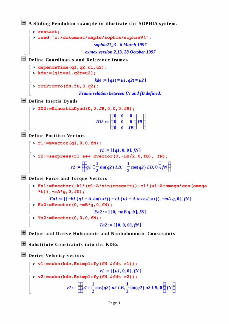
numeric analysis. In appendix 2, some of the most important functions in SOPHIA aredescribed briefly and a SOPHIA file of the “Sliding Pendulum” example from paper Eand F is also provided in this appendix. This file includes the various steps required toperform an analysis in SOPHIA and they are:

• Define generalised coordinates (q) and generalised speeds (u) as time dependent.The derivatives are denoted by an appended “t” (i.e. q1 → q1t and u1 → u1t). Therelationships between the coordinates and the speeds are also defined in thekinematic differential equations. See Equation (11).

• Define body fixed reference frames and auxiliary reference frames. The frames aredefined as a simple rotation from one frame to another frame about a frame axisand a given angle. The body fixed reference frames describes the orientation of thebodies in the mechanism.

• Formulating position vectors to the centre of mass for each body in the mechanism.This defines the geometry of the mechanism and the vectors are formulated interms of coordinates and parameters using the defined reference frames.

• Formulating the resultant applied force and moment vectors acting on each body.

• Derive the velocities from the position vectors and the angular velocities from thebody fixed reference frames. Prior to this step, if applicable, additional constraintsare formulated and substituted into the kdes to obtain velocities with includedconstraints.

• Derive differentiated linear and angular momentum vectors. Masses and momentsof inertia dyads must be introduced here.

• Construct KM-vectors for the velocities, forces and momentum, see Equation (1).

• Derive the tangent vectors from the velocity KM-vector and the specifiedgeneralised speeds. KMtangents computes this according to Equation (12) andreturns all the tangent vectors according to the specified generalised speeds.

• Derive Kane’s equations according to Equation (9). &Kane performs the fat dotproduct according to Equation (2) for all the provided tangent vectors and returnsthe symbolic equations of motion as a list of Maple equations.

• Export the equations as a mex-function for further numeric evaluation inMATLAB. The equations (Kane’s equations and the kdes) can be exported oneither implicit or explicit form. The state variables, the output derivatives of these,and the parameters are specified. Prior to exporting the equations, they areautomatically optimised by the introduction of intermediate variables that areevaluated once in the beginning of the numeric evaluation.

An advantage with SOPHIA is that the symbolic equations are immediately available in acomputer algebra system for further manipulation. Furthermore, there are no limitationsin SOPHIA since it assists the user in the Maple environment to perform MBS analysis.It is only a matter of building the desired expressions or equations using the availablefunctionality. The limitation is in the Maple system and how Maple handles the derivedsymbolic expressions.

19

The possibility of manipulating the equations of motion in SOPHIA and Maple prior toexporting them to Matlab is investigated in Paper D. The work focuses on the CPU-timerequired to perform the symbolic manipulations and the successive numeric evaluation inMatlab. The equations represent the motion of a four-bar mechanism and the differentsymbolic manipulations are:

• solve the equations to get them on explicit form or keep them on implicit form

• simplify the equations or keep them unsimplified

For each of the combinations of these manipulations one can either

• substitute the numeric values into the equations or keep the symbolic parameters

It is found in the paper that the implicit and unsimplified equations are the fastest toevaluate in the numeric domain. These equations also require the least manipulations inthe symbolic domain and are thus the fastest to derive in the symbolic world. One of thereasons for this result is probably that simplified expressions include more arithmeticoperations (e.g. simplification of (a+b)·c results in a·c+b·c, three operations instead oftwo). This limited study recommends that simplification is not performed on largeexpressions. In MBS analysis, expressions of the velocities (differentiated only once) arerelatively small but acceleration expressions (differentiated twice) tend to grove fast.Simplification efforts should thus be performed for velocity expressions but avoided foracceleration expressions.

2.5 Summary and conclusions

This chapter has discussed several methods for deriving equations of motion whereKane's method and the geometrical interpretation of these equations are the mostimportant for the remainder of the thesis. Traditional MBS software and the functionalityof those analysis tools have also been discussed in a general manner. Furthermore, theSOPHIA system, which is based on Kane’s method, is presented in more detail. ThisMBS software is used by MECHAMOS to derive symbolic expressions and further, theequations of motion on symbolic form.

The most important results from the discussion are the poor ability to search for MBS-data in traditional MBS software and the importance of symbolic and numericcapabilities simultaneously available in an MBS software. The latter offers assistance inderiving symbolic expressions and evaluating these numerically by reusing the symbolicinformation such as velocities and angular velocities etc. from the symbolic world whenperforming evaluation in the numeric world.

Both the increased ability to search for MBS-data and the symbolic/numeric capabilitiesare supported by the MECHAMOS system. This improve the MBS analysis as is seen inchapter 5 where MECHAMOS is presented.

20

21

3. Database Technology

The need for, and production of, large information quantities in many of today’s businessactivities require that the data is structured and that efficient searches of data arepossible. Database technology has developed strongly over the last decade to meet theserequirements. Consequently, databases become more and more important in softwareapplications and are used in many different fields of application. Most intuitive areapplications keeping record over employees, customers, phone numbers, car registrationsetc. These applications are characterised by fairly static data and, in some fields, largequantities of data. Other applications that involve more dynamic data are softwaresystems that continuously log data or register events. Some examples in this area are: asupermarket where all the items of merchandise are registered when delivered and sold;an industrial process where temperatures, fluid levels etc. are continuously logged; thebanking system where all the transactions are registered; the stock exchange where allthe stock trades are registered.

Introducing database technology in a field of operation usually facilitates and makes thedaily routines more efficient. As a bonus, strategic and important information can beextracted and derived from the data in the database. In the above supermarket example,the introduction of barcodes and thereby the ability to automatically detect and registeran article and its price, has reduced the work for and made the cashier more efficient.The database is automatically updated in a purchase and thus, at any instant, representsthe merchandise situation in the supermarket. Information that was impossible or tediousand costly to derive by hand can now easily be extracted and derived by searching thedatabase. For instance, the database system can detect articles that are low in stock andsearch for those that are selling well or return a large profit. Thus, in this example,database technology is a very powerful tool for monitoring the flow of articles throughthe supermarket. Information can be extracted that support decisions for improvementswhen it comes to routines or choice of products.

Common for most of the above exemplified business and administrative applications isthe relatively simple and uniform data with fixed length data fields in the database.However, in engineering applications, the data is more complex and requires moreadvanced operations to be performed on the data in the database. The intention with thischapter is to give an introduction to database technology, to sort out some conceptionsand look at the terminology in this field. The relational data model, suitable for businessand administrative applications is discussed and compared with the object-oriented (OO)data model, which is more suitable for engineering applications. Finally, the researchprototype database AMOS is described which falls in the category of object-relationaldatabase management systems.

The chapter is mainly based on Cattell [15] and Orsborn [1] where database technologyis more thoroughly discussed from an engineering point of view and extensive referencelists of database literature are provided. Orsborn's work is similar to the work in thisthesis but focuses on the use of database technology in finite element analysis. This thesisutilises database technology in multibody system analysis and a major differencecompared to Orsborn's work is the introduction of symbolic equations and symbolicmanipulations in the database.

22

The related appended paper to this chapter is paper C, which gives an introduction todatabase technology and further describes an early implementation of the MECHAMOSsystem.

3.1 Databases and database management systems

A database is just a collection of related data and can be as simple as an ordinary text filecontaining names and phone numbers. It is obvious that some sort of software is requiredto access the data in the text file. A database system (DBS) is a more complete softwaresystem for handling the data. The objective of a DBS is to provide users and developerswith generic software tools that support definition and manipulation of data in anefficient, uniform, flexible and secure manner. A DBS is illustrated in Figure 3 and itconsists of the following parts:

• A database where the actual data and the database schema is stored. Theinformation model, also referred to as the database schema, is a description ofhow the data is stored in the database. This description defines data types,relationships etc. and is expressed in terms of the data model supported by thedatabase management system.

• A database management system (DBMS). The DBMS is an intermediate softwarebetween users and the data in the database. It consists of one layer with datamanaging tools for accessing the database and one layer defining a databaselanguage. The language provides a generic interface between the database and theusers or software applications. This language is often referred to as a querylanguage. A powerful query language should include constructors for databasedefinition (i.e. the information model), data updating, and querying data in thedatabase.

• Software applications and interfaces interacting with the DBMS. Access andmanipulation of the database are done through the query language. It can either bedone directly by posing queries to the DBMS or indirectly through an applicationprogram, which interact with the database through the query language. In thesecond situation the user, maybe unaware, invokes predefined queries by choosingin menus, browsers or pressing buttons in the software application.

A DBS is an efficient mean to organise and share data in a multiple user environment.This put requirements on the DBMS to provide control functions on the data handling.For instance, the latest trend is to make data available and accessible via the Internet andeven banks let their customers access and manipulate the databases this way. Thecustomers cannot only monitor account balances but also order stocks and transfermoney between accounts. Some important general DBMS facilities to provide thecontrol functions and to obtain an efficient, powerful and secure DBS for multiple usersare:

• authorisation control which is responsible for the users accessibility of thedatabase. It can for instance restrict access privilege for a user, or a certain groupof users, to a specific part of the database. The access may also be restricted to asubset of database operations.

23

• data integrity control which is responsible for keeping the data within constrainedlimits.

• concurrency control which is responsible for preserving data consistency in amulti-user environment where several users might simultaneously access the samedata objects.

• backup and recovery which are responsible for keeping the data safe against failureby making persistent backups and keeping a log of database operations.

Figure 3 A database system consists of a database for persistent storage of data and the infor-mation model, a database management system (DBMS) for managing the database, and an in-terface or application software accessing the database language. Illustration from Orsborn [1].

Data models

The data model provides the DBMS with data types and data operators. There arebasically four different types of DBMSs if they are categorised by the underlying datamodel. The first two to appear were the hierarchical and network data models. They arebased on record types connected in a hierarchical tree structure and a network structurerespectively. Manipulation is accomplished by, in the host language, navigating the treeor network structures.

Next to appear were the relational data model. This data model is the most widely usedand has become very important, especially in business and administrative applications asexemplified above. These applications are characterised by large amounts of data with arelatively uniform and simple structure and the operations on the data are usually smalland simple. The reason for its success is probably the high-level query language availablefor data definition, retrieval, and update. SQL (the name stands for structured query

24

language) is an example of a general query language and it has become a standarddatabase language for relational database systems. The single data structure in therelational data model is the relation. Data is related in tables where the columns of thetable represent attributes and the rows represent tuples.

Engineering applications (and their models) usually require more complex data structuresand therefore demand specialised data types beyond the basic types supported in therelational data model (i.e. character strings, integers and floats). In mechanicalengineering typically vectors, matrices, coordinate systems etc. are important basic datatypes. Furthermore derived data is important in the engineering field and the analysismethods are usually of a complex nature including solving different types of non-linearequations. These calculations require advanced mathematical operations to be supportedby the data model. The object-oriented data model has a richer data structure comparedto the relational model and enables user-defined data types and operations in terms ofobject types and methods operating on these object types. Some of the object-orientedconcepts are:

• Objects. The objects are used to model physical or abstract entities that possesscertain characteristics and the object type structure should reflect the physicalsystem that is modelled as much as possible.

• Object types and inheritance. The named object types (also referred to as classes)are used to group objects with similar characteristics. These object types arerelated in a type hierarchy of subtypes and supertypes. Subtypes inherit definedproperties from their supertypes (if multiple supertypes are supported). The objecttype hierarchy and behaviour (i.e. methods) are important mechanisms forstructuring the data. This hierarchy adds knowledge to the database about thecharacteristics of the system being modelled and the inheritance reduces the codingefforts required to build the software application.

• Object identity and attributes. The object identity (OID) is a unique objectidentifier, usually a number, that is automatically generated by the DBMS when anobject is created. Properties of the objects are modelled as named attributes andare for example integers, reals, strings, arrays and references to other objectsthrough their OIDs.

• Methods and encapsulation. In addition to attributes, methods can be defined onthe different object types. A method is a named procedure or operator that definessome sort of computational algorithm involving attributes and other methods.Where and how the information is stored in the object structure is implemented inthe methods and this hiding of the internal data structure is called encapsulation.

• Overloading. The ability to define different methods with the same name but ondifferent object types is called overloading. This permits operators to have differentimplementations for different object types. The DBS decides which one of themethod implementations that should be invoked by the data type of the arguments.

Object database technology has evolved from two different fields. The object-orienteddatabase technology originated from the field of object-oriented programming languageswhere the need for database facilities evolved. Early products within this category had

25

limited querying capabilities and also lacked other general DBMS facilities. The object-relational database technology evolved from the field of relational database technologywhere the relational model was extended with object-oriented concepts to be able tohandle user-defined and more complex data types. This provides the object-relationaldatabase with an extensive SQL-like query language as well as other important DBMSfacilities.

Query language and data independence

The query language is the interface between the users or programmers and the database.It is thus important that this query language supports data definition, data retrieval anddata update. There are two important features of a query language, it provides Englishlike syntax and it provides data independence. The syntax simplifies database accesssince end users and programmers have minimal new language to assimilate. This lan-guage can also be domain-intuitive if the domain-specific concepts are named intuitively.

A relational complete query language must provide three basic operations [16]: selection,projection and join. In the relational data model selection produces a subset of the rowsof a table, projection produces a subset of the columns of a table and join matchesattributes from two different tables that have related values. In the OO data modelrelational complete corresponds to objects, object types and attributes.

Data independence is provided since high-level statements are automatically compiledinto low-level statements by the DBMS. Hereby, the user specifies what data are desiredand the DBMS determines how to get the data. This is called logical data independenceand the information model can be changed without having to change the application pro-grams that access the data in the database. On a lower level, physical data independencemeans that physically stored formats of records, indexes etc. can be changed withouthaving to change the information model. Data independence is important since storeddata is likely to change over time. If data independence is not provided, a small change inthe information model would most likely require significant changes in the applicationprograms.

3.2 The AMOS object-relational DBMS

AMOS (Active Mediators Object System) is a research prototype DBMS that falls in thecategory of object-relational DBMSs [1,2,18]. AMOS is a main-memory DBMSimplying that the entire database resides in primary memory. This is especially importantfor computational intensive applications where performance is critical and disk accesswould be to time-consuming. Furthermore, AMOS provides a relational complete querylanguage (AMOSQL) that is extensible and object-oriented with a declarative queryinterface for defining, populating and manipulating the database. Thus, searching andretrieving information from the database is done through the AMOSQL query language.This language has a similar syntax as SQL, which has become a standard language forrelational DBMSs. A typical AMOSQL query consists of three parts:

SELECT < define the data to be retrieved >FROM < define what object types to be involved in the retrieval >WHERE < conditions selecting the data that fulfil the constraints >

26

Examples of AMOSQL queries are found in chapter 4 where MBS analysis is performedthrough the query language in the MECHAMOS system.

To illustrate how an information model is defined through the AMOSQL language thegeneral domain concepts that are defined in MECHAMOS are taken as an example. Theinformation model for these concepts is illustrated in Figure 4, which is showing datatypes, inheritance and attributes. The general domain concepts are a set of basic datatypes for mathematical manipulation of numeric data and symbolic expressions. One veryimportant data type in MBS analysis is the vector data type and theeuclidean_vector object type in the information model represents this data type. Tocreate an object type (i.e. class) in AMOS the create type statement is used and theeuclidean_vector is defined with

CREATE TYPE geometric_object;

CREATE TYPE euclidean_vector SUBTYPE OF geometric_object;

Other general domain data types in MECHAMOS are as shown in Figure 4, dyads,reference frames, scalars and numeric sequences. The reference frames belong to aspecific model and as vectors and dyads are expressed in these reference frames, theyalso belong to the same model. It is thus, not possible to add two vectors defined for twodifferent models (i.e. expressed in different sets of reference frames). Numeric sequencesare used to represent scalars and vectors that are evaluated for different simulationresults. They consist of one numeric value for each time step of the integration. For moredetailed information on these data types, examples of instantiated objects are illustratedin Appendix B of paper C.

To represent attributes and methods in AMOS, it is possible to define functions asstored, derived, procedure or foreign through the AMOSQL. A stored function has itsextension explicitly stored in the database (attribute), whereas a derived function has itsextension defined in an AMOSQL query and a database procedure in an AMOSQLprocedure (method). The extensible capability of AMOSQL is an important functionalityto achieve a flexible DBS and to enable modelling of complex data and computationalmethods in the DBS. Due to the extensibility, foreign functions can be defined in anexternal programming language like C or LISP (or languages callable from these) andthese foreign functions are then available in AMOSQL as any other AMOSQL function.

The above vector data type consists of the three vector components and the referenceframe in which the three components represent the vector. The components are eithersymbolic expressions or numeric values and are stored as a three dimensional vector.This is modelled by the two stored functions representation and frame on theeuclidean_vector type and they are defined with

CREATE FUNCTION representation(euclidean_vector)-> VECTOR AS STORED;

CREATE FUNCTION frame(geometric_object)-> reference_frame AS STORED;

The stored function frame is a reference (contains an OID) to an object of typereference_frame and this object includes a full definition of the reference frame.

27

Figure 4 The information model for the scalar, vector, dyad, reference frame and sequenceconcepts as defined in MECHAMOS. Rectangles indicate object types, diamonds indicatereference attributes, ellipses indicate attributes and arrows indicate inheritance. Dashedrectangles indicate subtypes not yet implemented in MECHAMOS.

Derived functions in AMOS are exemplified by differentiation of a vector with respect totime and relative to the inertial reference frame. The function diffvec is defined on theeuclidean_vector type and returns a new object with the derived vector. Thefunction is created with

CREATE FUNCTION diffvec(euclidean_vector ev)->euclidean_vectorAS SELECT constr_evec(model(ev),l_diffvec(model(ev), evec_str(ev), name(irf(ev))));

This function consists of function calls to other defined functions. constr_evec is adatabase procedure that creates a new object of the type euclidean_vector and

28

instantiates its stored functions with the function update statements set , add andremove . The derived functions evec_str , model , and irf are defined on theeuclidean_vector type where model retrieves the OID to the model which thevector belongs to and irf retrieves the OID to inertial frame of that model. The storedfunction name is defined on the reference_frame type, se Figure 4, and thus,name(irf(ev)) retrieves the name of the inertial frame in which the vector is to bedifferentiated. Finally, l_diffvec is a foreign function defined in LISP that performsthe differentiation of the vector. The required data for the differentiation are retrieved bythe above described AMOSQL functions and passed as arguments to l_diffvec andfurther to MapleV and the SOPHIA system where the actual computation takes place.evec_str is here a special functions that puts the vector on a format suitable for theSOPHIA system.

There are different types of vectors in MBS analysis and this knowledge is modelled bydefining additional object types as subtypes to the euclidean_vector type, seeFigure 4. In AMOSQL, this is done with

CREATE TYPE position_vector SUBTYPE OF euclidean_vector;

CREATE TYPE velocity_vector SUBTYPE OF euclidean_vector;

CREATE TYPE acceleration_vector SUBTYPE OFeuclidean_vector;

These object types inherit the stored and derived functions defined on their supertypes(even multiple supertypes is supported in AMOS). However there is a differencebetween the above vector types when they are differentiated. The position vectordifferentiated yields a velocity vector and further differentiation of this vector yields theacceleration. This knowledge is modelled as an overrided function for the differentiation.Overriding is the same as overloaded except that overriding redefines an inheritedfunction rather than creating a new function with the same name but on another objecttype. Thus, changing the definition of the function diffvec for theposition_vector type to return a velocity_vector type is done with

CREATE FUNCTION diffvec(position_vector pv)->euclidean_vector AS SELECTconstr_velvec(model_oid(pv), l_diffvec(model_oid(pv),evec_str(pv), name(irf_oid(pv))));

where the only difference is that constr_velvec is used instead of constr_evec .

AMOSQL functions can not only be overloaded on one argument type but on all theargument types of the function, i.e. functions defined for different combinations ofargument types can share the same name. This functionality in AMOS facilitates theimplementation and the use of arithmetic operators (+, -, *, /) on different data types.Three of the data types defined in MECHAMOS are the scalar data type, dyadic datatype (3×3 matrix defined in a reference frame), and the above described vector data type,see Figure 4. These data types are defined for both symbolic expressions and numericdata. A multiplication operator is then defined on each of the data types and also on acombination of the data types. Different argument-type combinations require differentimplementations and yield different data types as results. For instance, multiplying twovectors is defined as the scalar product of the vectors and multiplying a vector with a

29

scalar is implemented as a scalar magnification of the vector. Table 1 presents theargument-type combinations for each arithmetic function (plus , minus , times , div )that are defined in MECHAMOS and their corresponding data type result.

The infix operators +, -, * and / are defined in AMOSQL as the functions plus , minus ,times and div . Hence, by overloading these functions on user defined data types, asdone in MECHAMOS, the infix operators are automatically available on the new datatypes. Which implementation of the function that is invoked in a function call isdetermined by the types of its arguments.

Table 1 also shows examples of the overloaded aggregation operator sum. Thesefunctions take a bag of vectors or scalars and sum all the objects in the bag. A bag is avery important AMOS type representing a collection of objects where the order of theobjects in the bag is not preserved. The results of AMOSQL queries are usually a bag ofobjects, which fulfil the constraints of the query.

Operation Functionname

Infixoperator

Resultingtype

s1 + s2 = s3 plus (s1,s2); s1 + s2; scalarv1 + v2 = v3 plus (v1,v2); v1 + v2; vectors1 - s2 = s3 minus(s1,s2); s1 - s2; scalarv1 - v2 = v3 minus(v1,v2); v1 - v2; vectors1 · s2 = s3 times(s1,s2); s1 * s2; scalars1 · v2 = v3 times(s1,v2); s1 * v2; vectorv1 · s2 = v3 times(v1,s2); v1 * s2; vectorv1 · v2 = s3 times(v1,v2); v1 * v2; scalarv1 · d2 = v3 times(v1,d2); v1 * d2; vectord1 · v2 = v3 times(d1,v2); d1 * v2; vectors1 / s2 = s3 div (s1,s2); s1 / s2; scalarv1 / s2 = v3 div (v1,s2); s1 / s2; vectorv1 × v2 = v3

cross(v1,v2); ---- vectorΣsi

sum(bag of s); ---- scalarΣvi

sum(bag of v); ---- vector

Table 1 Overloaded arithmetic operations defined in MECHAMOS. The AMOS functions(plus , minus , times , div ) are overloaded on the MECHAMOS data types scalars (s), vectors(v), and dyads (d). Hereby infix operators (+, - , * , / ) can be used on these MECHAMOS datatypes.

Rules and multi-directional functions

Some further features supported by AMOS are a rule handling system and the ability todefine multi-directional functions. The rule system consists of a condition part formonitoring changes in the database and an action part for executing operations triggedby certain events in the DBS. The available rule system classifies AMOS as an activeDBMS that automatically can react on database events or external events. In contrast, apassive DBMS requires that the user trigs all the actions.

30

Multi-directional functions are functions that can be applied for different bindingpatterns. A binding pattern defines which of the arguments and the results that are bound(known), and which that are unbound, in a function invocation. As an example, considerthe AMOSQL function sqrt(x) which takes the square root of x. The two AMOSQLqueries

AMOS 1> SELECT x FROM NUMBER x WHERE sqrt(4)=x;-2.02.0

AMOS 2> SELECT x FROM NUMBER x WHERE sqrt(x)=4;16

take the square or the square root depending on which of the function argument or thefunction result that is bound. Note that the first select statement is equivalent to thefunction call sqrt(4); . For stored, derived, and procedural functions, this multi-directional capability is automatically supported where applicable. In the case of foreignfunctions, the user must explicitly define the applicable variants of the multi-directionalfunction.


In this chapter database technology has been discussed in a general manner. The differentparts of a database system have been described briefly and the two most common datamodels were described and compared.

The relational data model has become very successful in business and administrativeapplications where the data is fairly simple and uniform. This has improved the ability tosearch and handle large data quantities in these software applications. The reason for itssuccess is probably the well-developed query language (usually SQL) that provides thedatabase system with a high-level general interface between the users and the database.

The OO data model offers a richer modelling capability compared to the relationalmodel. This makes the OO model more suitable for modelling mechanical systems wherethe data is more complex. In the OO model, data is modelled as object attributes, objectrelations, object type structure, and methods whereas in the relational model, the datastorage is restricted to attributes in different tables.

Conclusions from this chapter are the requirements on a DBMS to support an OO datamodel and provide a general query language that defines, populates, manipulates andsearches the database. The extensibility of such a query language is also very importantsince complex data and advanced operations then can be defined in a suitable foreignprogramming language. These requirements are met by AMOS and it is seen in thischapter that overloaded functions, also supported by AMOS, are a very powerfulconcept in defining arithmetic operators for different symbolic and numeric data types.Furthermore, the extensibility of the query language is also seen to be important assymbolic manipulation is not supported by the DBMS but can be defined in a foreignlanguage capable of symbolic manipulation.

31

4. The MECHAMOS Implementation

The concept of building software on top of standard database technology has success-fully been used in business and administrative applications. However, in engineeringapplications this concept is not yet common practice among the software developers. Aspointed out in chapter 2.4, the data management and ability to search for MBS-data arevery limited in traditional MBS software. In an attempt to improve this, an MBSsoftware, called MECHAMOS, that combines database technology and a traditionalMBS software has been developed. This approach provides the MBS software with datamanagement tools and the ability to search over the MBS-data. The idea is to store theMBS-model in the database as a minimal set of MBS base data on a neutral format.From this base data, other MBS-data is derived within the DBMS. Hereby it is possibleto search both over the stored MBS-models and over the derived MBS-data andsimulations results.

The purpose of this preliminary implementation of MECHAMOS is not to develop acompetitive ready-to-use MBS software. The objective is rather to show how MBSanalysis can be implemented in a database environment and to give an understanding ofhow modern database technology can improve the ability to search for MBS-data andhereby facilitate the MBS analysis and access of MBS-data.

This chapter continues with a description of the implementation architecture and how theMBS-data is stored in the database. Some examples are given on how MBS analysis canbe performed through the available query language.

Related appended papers to this chapter and the MECHAMOS system are:

• paper C where an early version of MECHAMOS is presented. The required basedata to enable MBS analysis is discussed and in the provided MBS example it isshown how MECHAMOS supports holonomic and nonholonomic constraints.

• paper D which studies the CPU time to derive the equations of motion on differentforms and further numerically evaluate these equations. The result of this study isimplemented in the strategy of deriving the equations of motion in MECHAMOS.

• paper E which shows how the query language can be used in MBS analysis. Thefull chain of operations required to derive different MBS-data is thoroughlydiscussed. Based on this, a simple materialisation handling is implemented inMECHAMOS that enables analyses involving several different simulations andeven several MBS-models.

• paper F where constraint force analysis based on Kane’s method is presented andimplemented in MECHAMOS. The provided MBS example shows how MBS-datais compared and combined for several MBS-models in the database.

4.1 The MECHAMOS architecture and data communication

The approach to perform advanced non-linear MBS analysis within a DBMS putrequirements on the DBMS to a) provide data types for representation of the MBS-

32

model, and b) be able to perform advanced mathematical operations. The mathematicaloperations are typically to derive ordinary differential equations (ODEs) on symbolicform that describes the motion of the mechanical system and then be able to solve theseequations using numerical methods. Thus, both numeric and symbolic manipulations arerequired by the DBMS.

To meet these requirements, the object-relational DBMS AMOS, described in theprevious chapter, is used as the base software. The AMOS DBMS provides an object-oriented data model with object-oriented concepts to describe the MBS-data and MBS-models. The extensibility of AMOS also enables mathematical operators to be defined ina foreign language. In MECHAMOS the mathematical capabilities of AMOS is extendedwith the full Maple functionality for symbolic manipulations and full Matlab functionalityfor numeric evaluation. Consequently, the SOPHIA MBS functions are also available inthe symbolic domain through Maple. With this architecture, illustrated in Figure 5,functions for advanced symbolic and numeric mathematical operations are integrated inthe AMOSQL query language.

Figure 5 The architecture of the MECHAMOS system. The AMOS DBMS is extended withMATLAB for numeric computations and MAPLE for symbolic manipulations. The files(indicated by a top right triangle) contain temporarily stored derived data used in thematerialisation handling.

33

The hart of the MECHAMOS system is, as seen in Figure 5, the MECHAMOS DBMSwhich is a 45 KB C-file that links together AMOS, Matlab and Maple. Executing this filefirst launches Matlab and Maple. The Maple workspace is then initiated with theSOPHIA system and finally, MECHAMOS enters the AMOS top loop. Hereby, the userinterface is a standard AMOS text window where interactive AMOSQL queries aremade.

All the foreign functions are also defined in the C-file as C-functions. These functions arerepresented by the close coupling4 in Figure 5 which is a direct data flow between twoprocesses. Data is passed from AMOSQL via LISP to these C-functions which furtherpasses the data to Maple or Matlab for the mathematical manipulation. Matlab is actuallyaccessed through the Matlab Engine which is a C interface to Matlab and is supplied withstandard Matlab. Standard Maple cannot be accessed from C and requires anothersoftware called MathEdge2 [20]. This software is basically the Maple Kernel, i.e. Maplewithout the graphical interface.

4.2 Base data and derived data

The information model of MECHAMOS is defined by making AMOSQL statements inthe MECHAMOS DBMS (approximately a 90 KB text file). This information model is adescription of the general domain concepts, described in the previous chapter, and theMBS domain concepts. These concepts are suitable for description and analysis ofmultibody systems in the SOPHIA system. The base data defined for the MBS domain,from which all the other MBS-data are derived, can be divided into data for themechanical system and data for each component in the system. Symbolic base data on thesystem level is listed in the top of Table 2 and are typically definitions of coordinates,reference frames etc. These attributes and references are defined in an object type calledmodel and the data is stored in terms of the general domain concepts presented inFigure 4 (e.g. euclidean_vector , reference_frame ). Symbolic base data oncomponent level are essentially the data required, for each body, to fully determineKane’s equations (9) (i.e. derive the system applied force vector, system momentumvector and the tangent vectors). This base data is listed in the bottom of Table 2 and theattributes and references are defined in an object type called body .

These two MBS domain concepts (model and body ) and their attributes are illustratedschematically in Figure 6. From the base data defined in the information model, it ispossible to derive symbolic expressions of velocities, momentum, energies etc. for thedifferent bodies. This is accomplished by utilising the vector algebra and vector calculusfunctions that are defined for the general domain concepts and described in the previouschapter, see for instance Table 1. Some examples of derived functions and theirdefinition on the object type body in the MBS domain are:

CREATE FUNCTION velvec (body b) -> euclidean_vector ASSELECT diffvec(posvec(b));

CREATE FUNCTION angvelvec (body b) -> euclidean_vector ASSELECT angvelvec(frame(b));

4 There are also loose couplings which is a file based data transfer between two processes. This is slowerthan the close coupling since it involves disc access.

34

CREATE FUNCTION linmom (body b) -> euclidean_vector ASSELECT mass(b) * velvec(b);

CREATE FUNCTION angmom (body b) -> euclidean_vector ASSELECT idyad(b) * angvelvec(b);

where the velvec function takes the position vector in the stored function posvec anddifferentiates it using derived functions for the general domain concepts. These examplesshow that the functions are fairly simple to implement and that they are declarative (i.e.the user specifies what data are desired and the DBMS determines how to get the data).The two momentum functions also illustrate the use of the overloaded infix operator ∗according to Table 1 in the previous chapter. Different user defined data types areinvolved in the multiplication where both a scalar (mass) and a dyad (idyad ) aremultiplied with a vector (velvec and angvelvec ).

Item Descriptionqj Number of generalised coordinatesuj Number of independent generalised speeds

( )� ,q f u qj = Kinematic differential equations[from,to,axis,angle] Definitions of reference frames

g Gravity vectormA Mass of the bodyr<A Position vector of the centre of massFa

<A Applied force vectorsJA Moments of inertia dyad in the centre of massfA Name of body-fixed reference frame

Ma<A Applied moment vectors around the centre of mass

Table 2 System and component level base data (above and below the line) in MECHAMOSdefined as stored functions on the model and body object types.

Figure 6 A schematic view of the information model for the MBS domain concepts as definedin MECHAMOS. Clouds indicate attributes and reference attributes defined on the object type.Other symbols are explained in Figure 4. Data defined on the system level is stored in themodel object and data on component level is stored in the individual body objects. The bodiesbelong to a model and arbitrary points can be defined in the bodies. Numeric data is stored inthe numeric objects and they also belong to a model .

35

Using various functions defined on the body and the model object types, the equationsof motion are derived by a sequence of SOPHIA statements (described in chapter 2.4and exemplified in Appendix 2). The required information (e.g. velocities, forces, andinertia) is selected from the database by making queries over the different bodies in theMBS-model. All this is defined in the function eom (and functions called by eom) whichreturns a mex-file containing the equations of motion on a suitable form for evaluation inMatlab.

CREATE FUNCTION eom (model m) -> CHARSTRING AS ......

Numeric MBS-data

To solve these equations of motion (i.e. non-linear ordinary differential equations),additional numeric information is required. This additional information is listed in Table 3and includes typically integrator settings, parameter and initial values. The data is storedin the numeric object type that is a part of the MBS domain concepts illustrated inFigure 6. Each of the instantiated numeric objects represents a set of parameter andinitial values defined for the MBS-model. On the numeric object type the ode23function is defined which feeds a MATLAB integrator (i.e. ode23 [21]) with thenecessary information to perform a simulation.

CREATE FUNCTION ode23 (numeric n) -> CHARSTRING AS ......

The result of this function is a sequence of numeric values for each of the coordinatesand their first time derivatives. In these sequences, there is one value for each time stepof the integration and the result is stored on a Matlab file.

Item Description Defaultt0 Start time of the integration 0t1 Stop time of the integration 5rel Relative tolerance 10-3

abs Absolute tolerance 10-6

refine Increases the number of integration output points 1initial Initial values of the coordinates and independent speeds 0parameter Numeric values of the parameter 1

Table 3 Numeric base data for numeric analysis in MECHAMOS defined as stored functionson the numeric object type.

An important feature in MBS analysis is to evaluate arbitrary symbolic expressions (sobelow) with a specific simulation result (n below) from the above ode23 function. Thecreated numeric sequence will then represent the time history of the expression for thisspecific simulation. In MECHAMOS this is done with the numseq function:

CREATE FUNCTION numseq (scalar_object so, numeric n) ->scalar_sequence AS ......

The result of this function is stored in an object type scalar_sequence which is a partof the general domain concepts illustrated in Figure 4. Symbolic expressions of

36

velocities, accelerations etc. of other parts of a body than the centre of mass isdetermined with the body_poi object, see Figure 6. This object defines the point ofinterest in a body as a vector from its centre of mass to the point. Derived functions aredefined on the object type to derive the symbolic expressions for velocities, accelerationsetc. This provides the user with assistance in formulating symbolic expressions fornumeric evaluation and further numeric analysis in MECHAMOS.

Materialisation

Deriving a numeric result from the MBS-model definition requires a chain of operationsthat is illustrated in Figure 1. This chain includes deriving the equations of motion (theeom function), numeric integration of the equations (the ode23 function) and numericevaluation of some symbolic expression in terms of the simulation result (the numseqfunction). In an MBS software like MECHAMOS where MBS-data is retrieved bymaking high-level AMOSQL queries on the MBS-model, the results should notdependent on previous queries, computations and definitions. To avoid this, the entirechain of operations must be performed for each query in the analysis. This implies that incomputational intense applications, like MBS analysis, reuse of previously computeddata is very important to achieve performance.

To meet these requirements, a simple materialisation handling has been implemented inMECHAMOS that monitors the most frequent and the most computational intenseoperations. Frequent operations are typically coordinate and frame definitions whereascomputational intense operations are to derive the equations of motion and to solve theseequations numerically. In general, materialisation is a DBMS concept that keeps track ofprevious posed queries and their result. If the same query is posed again, the previousresult is returned rather than derived again. This requires that the materialisation also canmonitor changes in the base data that influence the result of the query. This base datamonitoring functionality of the materialisation concept is not implemented inMECHAMOS.

The materialisation handling opens the possibility to pose queries in MECHAMOS thatcompare and combine MBS-data from several numeric parameter sets (i.e. differentsimulation results) and even from several MBS-models. Queries over different parametersets represent the ability to perform traditional parameter studies of a design. On theother hand, queries over different models represent the ability to compare an overallfunctional behaviour of a design where the different models represents different technicalsolutions to obtain the required functionality. Queries over several models can also repre-sent a comparison of different modelling techniques where the different models representthe same physical system or phenomena. Regardless of the analyses, the support for datamanagement in MECHAMOS together with the materialisation handling considerablyimproves and facilitates the MBS analysis. These issues of materialisation and AMOSQLqueries over several numerical sets are further discussed in the appended paper E.

Constraint force analysis in MECHAMOS

The present version of MECHAMOS utilises Kane's method to derive the equations ofmotion through the SOPHIA system. In this method constraint forces do not even haveto be defined to obtain a minimal set of constraint reaction-free equations. However, the

37

ability to determine the constraint forces is very important in MBS analysis and in Kane'smethod this is done after the motion has been determined. Instead of projecting theNewton-Euler equations (7) onto the tangent space as done in Equation (9), they areprojected onto the complementary space according to Equation (14). This method isdiscussed in paper F where it is found that by a proper choice of the complementarybase vectors, the equations that determine the constraint forces are uncoupled in theconstraint forces (i.e. each additional equation only contains one unknown constraintforce).

The base data required for this analysis is listed in Table 4. The constraint force vectorsare defined and a fictitious coordinate is introduced in the direction of each definedconstraint force. These additional degrees of freedom require the definition of anadditional position vector from which the complementary base vectors are derived. Fromthese base data it is thus possible to derive the system constraint force vector and thecomplementary base vectors and hereby symbolic expressions and numeric sequences ofthe constraint forces can be derived with Equation (14).

The advantage with this approach is the simplicity in formulating the required equationsto determine a requested constraint force. In the database it is enough to keep track ofwhich fictitious coordinate that corresponds to the constraint force. Then thecorresponding complementary base vector is formulated and the single equation thatdetermines the constraint force is derived.

Item DescriptionNi Name of the generalised constraint forcesqfi Name of the associated fictitious generalised coordinates

[from,to,axis,angle] Definition of associated fictitious reference framesr f

<A Additional position vectors due to fictitious displacementsFc

<A Constraint force vectorsM c

<A Constraint moment vectors around the centre of mass

Table 4 Additional base data on system and component level (above and below the line) toenable constraint force analysis in MECHAMOS. These items are defined as stored functionson the model and body object types.

Holonomic and nonholonomic constrains in MECHAMOS

To enable MBS analysis of a wider class of problems in MECHAMOS, additionalconstraints imposed on the mechanism must also be stored as base data. From thediscussion in chapter 2.3, holonomic (geometric) and nonholonomic (velocity)constraints are treated similarly by expressing the dependent generalised speed asfunctions of the independent generalised speeds, Equations (24) and (25). Theseconstraints must be substituted into the velocity expressions to obtain correct tangentand complementary space base vectors (β j

< and γ i< respectively).

Table 5 lists the base data required in MECHAMOS to handle these additionalconstraints. Expressions of the dependent generalised speeds, as expressed in Equations(24) and (25), are stored in the database for deriving proper tangent vectors. To obtain aproper set of complementary base vectors, additional constraint expressions that include

38

the fictitious coordinates and velocities are also stored. Finally time dependentconstraints are stored to allow coordinates and parameters to be expressed as knownfunctions of time and hereby obtain correct differentiated expressions.

Item Description( )α = f t Time dependent functions and parameters

( )u f u qholo indep= , Generalised speeds subjected to holonomic constraints

( )u f u qnonholo indep= , Generalised speeds subjected to nonholonomicconstraints

( )u f u q q qholo indep f f= , , � , Generalised speeds subjected to holonomic constraintsincluding fictitious coordinates for constraint force analysis

( )u f u q q qnonholo indep f f= , , � , Generalised speeds subjected to nonholonomicconstraints including fictitious coordinates for constraintforce analysis

Table 5 System level base data in MECHAMOS for additional constraints on the mechanicalsystem. These items are defined as stored functions on the model object type.

4.3 Using the AMOSQL query language in MBS analysis

In this section, the above description of MECHAMOS is illustrated with some examplesof how MBS analysis is performed through the AMOSQL query language. There aresome features in a DBMS based MBS software, such as MECHAMOS, that are notalways available in a traditional MBS software. The objective with the followingAMOSQL examples is to illustrate some of these features, namely:

• a higher level of the MBS analysis with a declarative nature of the query language.The user specifies what data to be retrieved and MECHAMOS knows how toderive that data.

• combination of symbolic and numeric data. MBS-data is hereby reused throughthe analysis phases.

• combination of numeric data from several simulation results. This high-levelparameter studies are practically impossible without the implementedmaterialisation handling.

• combination, searching and comparison of MBS-data from several MBS-models.

Another purpose with the examples is to show that MECHAMOS can handle certainclasses of problems in a general manner. The crank-roller example in paper C illustrateshow holonomic and nonholonomic constraints are treated in MECHAMOS whereas timedependent constraints are illustrated by the sliding pendulum example in paper E andconstraint force analysis are illustrated by the friction pendulum example in paper F.These three models are illustrated in Figure 7 where the sliding and friction pendulummodels only differ in the existence of friction between the slider and the ground. A moredetailed discussion on the MBS-model base data for these examples are given in thecorresponding appended papers. The input text-files that populate the MECHAMOSdatabase with the MBS-model base data are also appended in each of the three papers.

39

Figure 7 Three simple examples representing different classes of problems: a) the crank-rollerand b) the sliding pendulum and friction pendulum. The bodies are named A, B and C aftertheir body fixed reference frames. In the friction pendulum model, there is assumed to be africtional force between the slider and the "ground surface".

For the below AMOSQL examples, it is assumed that MECHAMOS is launched and thatMBS-models for at least the above three examples are available in the database.Furthermore, there are no pre-computations, initiations, or definitions required for any ofthe below examples. All the necessary computations are performed within each query.The first example retrieves the symbolic vector of the angular velocity for body B (withthe body fixed reference frame b1b2b3) in the crank-roller model. This is formulated inthe high-level query language AMOSQL as:

MA1> SELECT angvelvec(b)FROM body bWHERE name(b) = "B" AND name(model(b)) = "Crank-Roller";

OID[0x0:2474]

MA2>

The declarative nature of the query language is reviled since the query only specifieswhat data to be retrieved and MECHAMOS knows how to retrieve the data. The resultis an object (with reference OID[0x0:2474] ) of the type euclidean_vectorcontaining the angular velocity vector and the reference frame in which it is expressed,

MA2> representation(OID[0x0:2474]);

{"0,0,-L1*u1*cos(q1)/(L2*cos(q2)}

MA3> name(frame(OID[0x0:2474]));

"fB"

MA4>

The above query is entirely operating in the symbolic domain and is an example of Phase4a of Figure 1. To create a graphical representation of the angular velocity in terms of aplot (Phase 4c), requires that both symbolic and numeric data are combined. In the nextexample, the data to be combined are the symbolic expression of the third component ofthe above vector (Phase 4a) evaluated for some numeric simulation result (Phase 4b).

40

The following query retrieves a numeric_sequence object that numerically representsthe time history of that vector component:

MA4> SELECT numseq(zcomponent(OID[0x0:2474]), n)FROM numeric nWHERE name(n) = "s20" AND name(model(n)) = "Crank-Roller";

OID[0x0:2478]

MA5>

This analysis requires that the equations of motion are derived (Phase 2) and that theseequations are integrated numerically (Phase 3) for the set of parameter values nameds20 . The numseq function in MECHAMOS does this automatically and then evaluatesthe symbolic expression for the simulation result. Assuming that the OID[0x0:2480] isa numeric_sequence of the time steps for the same integration, the graph in Figure 8is obtained by

MA5> plot(OID[0x0:2480],OID[0x0:2478]);

MA6>

Figure 8 is obtained by the above sequential set of queries. This graph can also begenerated, without relying on intermediate query results, by the single query

MA6> SELECT plot(zcomponent(angvelvec(b)),n);FROM body b, numeric nWHERE name(b) = "B" AND name(model(b)) = "Crank-Roller" AND name(n) = "s20" AND name(model(n)) = "Crank-Roller";

MA7>

0 5 1 0 1 5- 8

- 6

- 4

- 2

0

2

4

6

8

A n g u l a r v e l o c i t y v s . t i m e

Figure 8 The angular velocity of body B about the n3-axis in the crank-roller example.

41

The plot function is also an example of an overloaded function. The argument types atMA5> are two numeric_sequence objects ready to be plotted. At MA6>, thearguments are a symbolic_scalar and a numeric where the latter defines thenumeric parameter values for the integration and the former is the symbolic expression tobe evaluated with the simulation result.

This angular velocity example clearly shows the improvement of MECHAMOS due tothe simple materialisation handling presented in paper E. The same example is presentedin paper C (section 5.5) where an early version of MECHAMOS required a set ofsequential commands to achieve Figure 8. The MBS analyses in paper C are thusdependent on the history of manipulations and definitions in the database which is not thecase in the above example (MA6>).

Next example illustrates the ability to combine numeric data from several simulations,which originate from different sets of parameter values. In the sliding pendulum modelthere are 31 different sets of parameter values defined with the oscillation frequency ofthe moving wall (ω) varying between 0 and 4 rad/s (note that there are only 29 setsdefined for the same example in paper E). The plot in Figure 9 shows the maximumamplitude of the pendulum angle (q2) for different ω-values and it is obtained by the twoqueries

MA7> SELECT applot_o("omega", max("q2",n), n)FROM numeric nWHERE name(model(n)) = "Sliding Pendulum";

MA8> SELECT applot_x("omega", max("q2",n), n)FROM numeric nWHERE name(model(n)) = "Friction Pendulum";

MA9>

When the first query (MA7>) is processed, 31 simulations are performed and theequations of motion are derived once since the materialisation handling detects that thederived equations can be reused for all the simulations. The second query above (MA8>)does the same thing but for the friction pendulum model.

The final example illustrates searching and combining numeric MBS-data from twodifferent MBS-models which, of course, are in some sense comparable. Figure 9 revealsthat the maximum amplitudes for the model without friction in general exceeds theamplitudes for the model with friction at the corresponding ω-values. For some ω-values,however, the reverse is true. Finding these ω-values and the amplitudes for the twomodels is done with the query

MA9> SELECT <value("omega",n1), max("q2",n1),max("q2",n2)>FROM numeric n1, numeric n2WHERE name(model(n1)) = "Sliding Pendulum"AND name(model(n2)) = "Friction Pendulum"AND value("omega",n1) = value("omega",n2)AND max("q2",n2) > max("q2",n1);

<0.5, 0.112536, 0.140174><0.7, 0.191865, 0.495814>

42

<0.4, 0.0798118, 0.0912223><0.6, 0.150273, 0.239334>

MA10>

When this query is processed the materialisation handling detects that the requiredsimulation results already exists (from MA7> and MA8>) and are therefore reused insteadof derived again.

0 0.5 1 1.5 2 2.5 3 3.5 40

0.5

1

1.5

2

2.5

Figure 9 The maximum values of the pendulum angle (q2) versus the forced oscillationfrequency ω for all the numerical sets defined in the MBS-models "Sliding Pendulum " (o)and "Friction Pendulum " (x ).

All the queries and the derived functions used in these examples are implemented in ageneral manner. They can be combined with other functions and applied on any relevantMBS model defined in the MECHAMOS database. It is only a matter of specifying, inthe SELECT clause, what data to be retrieved and, in the WHERE clause, put relevantconstraints on the selected data.

In traditional MBS software, the analyses performed in the last two examples (MA7> toMA9>) would most likely require extensive programming efforts. This program usuallyadministrates the analyses by feeding the integrator with correct parameter values,storing intermediate results, analysing the data, keeping track of which result is storedwhere etc. These programs can be reused, but that requires recoding as the programstend to be analysis and model specific rather than general.

43


In this chapter, the MECHAMOS system for MBS analysis has been described. Thearchitecture with the AMOS DBMS, Matlab, Maple and SOPHIA has been discussedand the required base data for MBS analysis was presented. MECHAMOS is based onKane's method for deriving the equations of motion which yields a minimal set ofconstraint reaction free equations in a minimal set of coordinates. This means thatMECHAMOS produces a minimal set of data and, because of the available symbolic andnumeric capabilities, further MBS-data is derived if and when required.

MECHAMOS supports different classes of problems in MBS analysis includingholonomic and nonholonomic constraints, time dependent constraints, and constraintforce analysis. The implemented method for constraint force analysis requires only oneequation to determine a constraint force. This simplifies the data management in theanalysis and, again, MBS-data is derived when required.

The provided query examples show how MBS-data can be retrieved on both symbolicand numeric form. The analysis is performed through the high-level query languageAMOSQL and the queries are fairly intuitive and of a declarative nature. The lattermeans that MECHAMOS automatically derives the equations of motion and/or performsa simulation if this is required to answer a query. In the last two examples it is alsoshown how MECHAMOS can combine and compare numeric data from severalsimulation results originating from two different but comparable MBS models.

The conclusion made from this chapter is that the available database technology inMECHAMOS considerably improves and facilitates the MBS analysis. The ability tointeractively search and retrieve MBS-data, both symbolically and numerically, fromseveral MBS-models through the general query language moves the analysis to a higherlevel and requires no or very little programming efforts5. Another key factor for theimproved MBS analysis functionality is the implemented materialisation handling. Thismaterialisation handling is crucial to achieve reasonable performance when searchingover several MBS-models as computational intense results (i.e. equations of motion andsimulation results) are reused when appropriate.

5 If the AMOSQL query is viewed as a small program, there is a small programming effort required,otherwise there is not.

44

45

5. Summary of Papers

This thesis includes six appended papers, A to F, that are summarised in this chapter.Paper A discusses the theory of systems and flow approach and paper B presents animplemented system for submodel techniques based on paper A. Papers C to F all relateto the MECHAMOS system and present different parts of MECHAMOS as theimplementation has evolved.

Paper A: A Functional Interpretation to Constrained Motion of Systems.

The purpose of this paper is to introduce a general structure for functional modelling ofmachine elements and mechanical systems. The approach was to relate a systems andflow approach for technical systems to multibody system analysis and Kane's equationsof motion in particular. With systems approach, it is meant that technical systems arelooked upon as an assembly of elements, characterised by the function of the elementsand the configuration of the assembly. The flow approach means that the flow of energy,material and information through the boundary of the volume and within the system arestudied and formulated.

Main finding is that the energy equation projects the Newton-Euler equations on to thetangent space in the same manner as Kane’s method. The equations of motion areextracted from the energy equation by a partial differentiation with respect to thegeneralised speeds. Furthermore, four basic functions are identified and formulated. Thefunction of any system or element, i.e. both the main and the secondary functions, can besplit up into these basic functions which are: to store something; to transform or convertsomething; to transport something; and to support something. In the paper threeexamples of different basic functions are formulated as submodels and finally thesesubmodels are assembled to form a simple flywheel suspended by a spring.

The main contributions of this paper are a) the identification of the equations of motionfrom the energy equation and b) the manipulation of the energy equation whenassembling submodels.

Paper B: DYMAP - A Dynamic Modular Assembly Package.

In this paper the modelling principles discussed in paper A are implemented in Maple Vas a package called DYMAP. The idea with DYMAP is to have a library of subsystemswhich are modelled in advance. These submodels are then assembled in DYMAP to forma model of the complete mechanical system. The submodels are stored in the library astext files where the functional description of the system is represented by the energyequation on symbolic form and the ports are defined by their velocity and accelerationvectors.

The kernel of DYMAP is a set of user routines implemented in Maple V to manipulatethe symbolic expressions defining the submodels. Main features are to read and storesubmodels in the library and further assembling submodels through pre-defined ports.When the assembly is satisfactory the equations of motion are extracted explicitly for the

46

system. In the provided example, two submodels are defined, a rigid body and a revolutejoint. The submodels are unconstrained prior to an assembly and therefore they have sixand seven degrees of freedom respectively. Based on these two submodels a doublependulum is assembled. The degrees of freedom of the submodels are then reducedbecause of the constraints imposed on the submodels and consequently the equations arereduced to describe a double pendulum.

The main contribution of this paper is the implementation and evaluation of the DYMAPsystem for assembling submodels.

Paper C: A System for Multibody Analysis Based on Object-Relational DatabaseTechnology.

This paper gives a fairly detailed presentation of an early version of MECHAMOS. Thesoftware architecture and defined object types are discussed and examples are given onhow to define types and functions in the available query language AMOSQL. On thetheoretical side, database technology is discussed as well as Kane's equations of motion.The required base data for MBS analysis is also thoroughly discussed. A crank-rollermechanism illustrates how the database is defined, populated and manipulated throughthe stored and derived functions. The MBS-data is retrieved on symbolic and numericform where the latter is based on numeric results from simulations of the symbolicequations of motion. This version of MECHAMOS supports the analysis of mechanicalsystems subjected to additional constraints as holonomic, nonholonomic and time-dependent constraints.

The main contribution of this paper is the MECHAMOS system which is a researchprototype for MBS analysis where modern database technology is utilised to store andaccess data. Hereby MBS-data is retrieved through a general query language.

Paper D: Computational Efficiency of a Four Bar Mechanism in MapleV andMatlab.

This paper investigates the CPU-time required to derive the equations of motion for afour-bar mechanism and evaluate these equations numerically. The equations are put intodifferent forms prior to the numeric evaluation. The equations can either be on implicit orexplicit form, simplified or unsimplified, and on symbolic or numeric form. Theseequations are then optimised using the standard Maple function optimize and exportedto a Matlab mex-file.

Main findings are that the standard Maple simplification command (simplify )performs well on small expressions but is very time consuming for large expressions.Further, the optimisation command performs better on the unsimplified expressions andthe numeric evaluation is found to be faster for these unsimplified expressions. This isonly done for a four-bar mechanism with one degree of freedom. However, it can beexpected that similar results will be obtained for other mechanisms as well. Theconclusion from this is that expressions up to the first derivative (e.g. velocities) shouldbe simplified where as second derivative expressions (e.g. accelerations) should be leftunsimplified.

47

The main contributions to the MECHAMOS system from this paper are a) simplificationof symbolic expressions does not always speed up the numeric evaluation of the sameexpression and b) finding which steps in the process of deriving the equations of motionthat should be simplified and which should not. These results have been implemented inthe MECHAMOS system to improve the computational performance of the system.

Paper E: Using an Extensible Object-Oriented Query Language in MultibodySystems Analysis.

This paper focuses on the use of a high-level query language in MBS analysis. With thisperspective, the entire chain of required computations to retrieve various MBSinformation is thoroughly discussed.

Main findings in the paper are that the entire chain of computations must be performedin each query to avoid dependency on previous queries and the existence of certainresults and definitions. In computational intense applications such as MBS analysis it isinconvenient to perform the same computations several times such as the numeric solvingof the equations of motion. It is thus important that the software support the concept ofmaterialisation. In this paper a simple materialisation handling has been implementedcovering the most computational intense operations and the most frequent operations.This enables MECHAMOS to query over several sets of parameter values and/or severaldifferent MBS-models. A simple example illustrates how a single query in MECHAMOSautomatically derives the equations of motion, solves these equations for 29 different setsof parameter values (29 simulations), and combines these results in a graph. Theconclusion is that the available DBMS provides MECHAMOS with general tools toautomatically perform parameter studies and the ability to search for MBS-data overseveral sets of numeric parameter values and over different MBS-models.

The main contributions to the MECHAMOS system from this paper are a) theincorporation of the entire chain of operations in the derived functions, b) theimplemented simple materialisation handling, and c) illustrating how MBS-data can besearched, compared and combined with the available database technology.

Paper F: Multibody Systems: Constraint Force Analysis through an ExtensibleQuery Language.

In this paper Kane's method for determining constraint forces is transformed to Lesser'sgeometric interpretation of Kane's equations and the concept of system vectors. Theconstraint forces are then determined by projecting the Newton-Euler equations onto thecomplementary space rather than onto the tangent space which yields the equations ofmotion. This method is then implemented in MECHAMOS to improve the constraintforce analysis compared to the early implementation in paper C. The base data isreduced from the actual expressions of the constraint force to data defining thecomplementary base vectors.

Main findings are that projecting the Newton-Euler equations onto certain directions inthe complementary space yields one unknown constraint force per equation. Thus, theobtained set of equations is uncoupled in the constraint forces. This facilitates the data

48

management in the analysis as only one equation has to be formed to determine a singleconstraint force. The constraint force example in this paper is the same as in paper E,with a friction force added. Hereby, two comparable MBS-models, describing the samephysical system, are available for analyses in MECHAMOS. It is shown in the paper howMBS-data for these two MBS-models are searched, compared and combined through thequery language.

The main contributions of this paper are a) implementation of a more general datastructure to store constraint force base data in MECHAMOS and b) obtaining equationsthat are uncoupled in the constraint forces in the same manner as Kane does but utilisingthe concept of geometric interpretations and system vectors from Lesser.

49

6. Concluding Remarks

The research work presented in this thesis has combined functional modelling of machineelements and mechanical systems with multibody system analysis and databasetechnology. The functional modelling is based on the systems and flow approach wherethe system behaviour is modelled by formulating the energy flow through the system. Itis seen in paper A that the energy flow is projecting forces and momentum onto thedirections of motion in the same manner as Kane's equations and the close relation tomodern MBS methods is established.

The introduction of database technology has resulted in the unique implementedprototype software for MBS analysis named MECHAMOS which merges the AMOSDBMS and the SOPHIA MBS software. The objective with this implementation hasbeen to investigate the potential benefits of integrating a database management systemwith MBS software in the same manner that has been successfully done for business andadministrative applications.

It is clearly shown in the examples that this approach, making data managing toolsavailable in the MBS software, considerably improves the analysis of technical systems.There are two key factors for this improvement, the available DBMS that providesMECHAMOS with a query language and the implemented materialisation handling. Thequery language is a general interface to the data and because of its declarative nature incombination with the materialisation handling, the analysis is brought to a higher level. InMECHAMOS, the desired data is specified, fairly intuitively, in a query and the DBMSknows how to retrieve and automatically derive that data. Thus, the user does not haveto specify the required sequence of operations to obtain the desired data.

Another important improvement is the ability to search over stored and derived data inthe database. This ability is not restricted to a single MBS-model, it is also possible tosearch, combine, and compare data from several models. This enables MECHAMOS notonly to perform a traditional parameter study over a parameter space within the sameMBS-model (i.e. varying parameter values). It is also possible to compare and evaluatedifferent technical concepts (i.e. different MBS-models) through the query language. Inthe provided examples, this was done for two different behaviour models (with andwithout friction) describing the same physical system.

The MECHAMOS system is implemented in a general manner supporting differentclasses of MBS problems. It utilises general database technology and an available MBSanalysis software. This MBS software was the SOPHIA system but other MBS softwarecould as well be used to perform the analysis (e.g. ADAMS, NEWEUL). The importantissue is that the data should be available in the DBMS on a neutral format. Powerful datamanaging tools can then be used to manipulate and analyse the data. In fact, havingseveral analysis tools available as computational engines in MECHAMOS, the mostsuitable software for a particular analysis can be used for the analysis. This putsrequirements on the model in MECHAMOS to be on a neutral and general format toenable other software specific models to be created from the base data. With thisapproach, the dependency on software developers is drastically reduced. For instance,changing software supplier only requires an interface between MECHAMOS and the

50

new software. When this is accomplished, all the models in the database are immediatelyavailable in the new software.

There are also benefits in sharing and reusing data between different application domains(e.g. CAD, FEM, CFD, MBS) in an engineering information system. The data is storedin a neutral format and all data is available through the declarative query language. Thismakes it easy to combine and transform the data to a suitable form for further analysis.Furthermore, the object-oriented environment and the available data management systemalso facilitate the software development and maintenance. General database functionalityis available to the implementation and thus, does not have to be specifically implemented.For instance, introducing new data types will automatically be handled by the DBMS andthere is no need to re-code the storage and search mechanisms in the implementation.

Further research

This work has investigated and evaluated new ideas in MBS software implementation.Naturally, the implemented system is in constant development and as the system evolves,more insight is gained on how it should be implemented. Therefore, a lot ofimprovements can be made and the list of future work is extensive. The number ofanalyses and the classes of problems supported by the system can of course be increased.The former is typically qualitative analysis to enable linearisation, stability analysis,determining eigenvalues etc. whereas the latter could be the ability to modeldiscontinuous systems with hard stops, impacts etc. However, more interestingimprovements are probably in the data management area and the ability to search overMBS-data.

In the present version of MECHAMOS, it is not possible to do a topological search ofthe mechanism finding the bodies that are connected to a specific body. Theseinterrelations are implicitly stored in the position vectors for the bodies and are thushidden from the DBMS. This can be improved by introducing a more submodel orienteddata representation where the objects (bodies or joints) refer to other objects that areconnected to them. It would then be possible to search the topological layout andretrieve the objects that are connected to a given object.

In an effort to make the analysis more intuitive, increase the ability to search, and put lessrequirements on the user to have specific knowledge about the MBS-model, the MBSdomain structure must reflect the physical system as much as possible. In the presentversion of MECHAMOS there are limitations in data retrieval due to the object typestructure. For instance, take the friction pendulum example in paper F and assume thatthe friction force on body A is to be retrieved. This is accomplished with the followingworking procedure:

MA> SELECT aforvec(b)FROM body bWHERE name(b) = "A"AND name(model(b)) = "Friction Pendulum";

OID[0x0:1636]OID[0x0:1640]OID[0x0:1642]

51

The results of this query are three applied force vectors acting on body A where one ofthem is the desired friction force vector. This vector is finally retrieved by a traditionalinspection of the three objects. Hereby, the friction force can not be searched for in anefficient way in the present version of MECHAMOS since the friction is not explicitlypresent or have an appropriate data type. This knowledge is now hidden in the moregeneral applied force vector of body A. With an extended object type structure thevector could be retrieved with the below query where specific knowledge about thefriction force is not required from the user.

MA> SELECT friction_force(b)FROM body bWHERE name(b) = "A"AND name(model(b)) = "Friction Pendulum";

OID[0x0:1640]

The conclusion from this is that the object types and function names should be extendedand changed to achieve an intuitive language for the analysis and enable efficient searchesand retrieval of MBS-data. MECHAMOS concepts must thus be extended to includeconcepts as friction force, spring force, etc. Also, a submodel oriented approach wouldenable an even more specific retrieval of the friction force. The force between body Aand the "ground surface" could be retrieved whereas the above query only yields the totalfriction force applied to body A.

Functional modelling and submodel techniques are discussed in paper A and these ideasare implemented in the software DYMAP presented in paper B. In DYMAP thedescription is based on the energy equation (17). When assembling submodels, theenergy equations from each submodel are summed and this expression is reduced due tothe constraints imposed on the submodels in the assembly. With a software likeMECHAMOS, where the equations of motion are derived from simple base data, thesubmodels (containing an arbitrary number of bodies with several degrees of freedom)should be defined in terms of some base data instead. Hereby the MBS-model isgradually built up by assembling suitable pre-defined submodels stored in the databaseand the equations are derived from scratch rather than obtained by reducing largeequations as in DYMAP. The assembled configurations could then be analysed in usingthe available query language. If an automatic assembling strategy is introduced it ispossible to make queries over a set of submodels. The query will then automaticallyassemble different combinations of the submodels and may retrieve the assembly that insome sense best meet some specified requirements. MECHAMOS could then act as anassistant to the designer in choosing standard components and machine elements basedon advanced dynamic analysis.

52

53

7. References

1. Orsborn, K., On extensible and object-relational database technology for finiteelement analysis applications, Ph.D. Thesis, Thesis No. 452, ISBN 91-7871-827-9,Linköping University, Sweden, October 1996.

2. Fahl, G., Risch, T., Sköld, M., AMOS - An Architecture for Active Mediators, TheInternational Workshop on Next Generation Information Technologies and Systems(NGITS'93), Haifa, Israel, June 28-30, 1993, p 47-53.

3. Lesser, M.B., SOPHIA, A Proscriptive Language for Mechanics, Proceedings ofthe 36th SIMS Simulation Conference, Stockholm 1994.

4. Lesser, M.B., A geometrical interpretation of Kane's Equations, Proc. of the Roy.Soc. London. A436, 69-87, 1992.

5. Lesser, M.B., The Analysis of Complex Nonlinear Mechanical Systems, AComputer Algebra Assisted Approach, World Scientific Publishing Co. Pte. Ltd.,ISBN 981-02-2209-2, Singapore, 1995.

6. Scheck, F., Mechanics, From Newton’s Laws to Deterministic Chaos, Springer-Verlag, 1990.

7. Essén, H., BASIC MECHANICS The science and it applications, Department ofMechanics, KTH, Stockholm, 1993.

8. Kane, T.R., Levinson, D.A., Dynamics: theory and applications, McGraw-HillBook Company, New York, 1985.

9. Lindsay, R.B., Margenau, H., Foundations of Physics, John Wiley & Sons Inc., 6th

printing, 1949.

10. Pahl, G., Beitz, W. Engineering Design - A Systematic Approach, Springer-Verlag,1988.

11. Andersson, S., Hugnell, A.B.J., Functional Modeling in Mechanical EngineeringDesign, International Conference On Engineering Design, ICED 91, Zurich, August27-29 1991.

12. Sharp, R.S., Multi-body dynamics applications in vehicle engineering, Proc.IMechE, Multi-body Dynamics: New Techniques and Applications, London,December 10-11 1998, pp 215-228, Professional Engineering Publishing, ISSN1356-1448, ISBN 1 86058 152 8, 1998

13. Sayers, M.W., Symbolic Computer Language for Multibody Systems, Journal ofGuidance, Control, and Dynamics, Vol 14, No 6 Nov/Dec 1991.

14. Lennartsson, A., Efficient Multibody Dynamics, PhD thesis, Royal Institute ofTechnology, Stockholm, Sweden, June 1999, TRITA-MEK 1999:01, ISSN 0348-467X.

15. Cattell, R.G.G., Object data management: object-oriented and extended relationaldatabase systems, Addison-Wesley publishing company, ISBN 0-201-54748-1,1994.

54

16. Date, C.J., An introduction to database systems, Addison-Wesley publishingcompany, ISBN 0-201-19215-2, 1987.

17. Bertino, E., Martino, L., Object-oriented database systems, Addison-Wesleypublishing company, ISBN 0-201-62439-7, 1993.

18. Flodin, S., Karlsson, J., Orsborn, K., Risch, T., Sköld, M., Werner, M., AMOSUser’s Guide, EDSLAB, Linköping University, Linköping, 1997.

http://www.ida.liu.se/labs/edslab/amos/amosdoc.html.

19. MapleV (release 4) is a registered trademark of Waterloo Maple Inc., 57 Erb StreetWest. Waterloo, Ontario Canada N2L 6C2.

20. MathEdge2 (MapleV application development engine) is a registered trademark ofWaterloo Maple Inc., 57 Erb Street West. Waterloo, Ontario Canada N2L 6C2.

21. Matlab (version 5) is a registered trademark of The Math Works Inc., 24 Prime ParkWay, Natick, MA 01760-1500.

55

Appendix 1. Notation and Abbreviations

In this appendix, notations and abbreviations used in the thesis are listed. A generalnotation used is that scalars are typed in italic, vectors in boldface, and dyads inunderlined boldface. Furthermore, the courier new font is used in the text forimplemented software data types , functions , etc.

The below list of notations is not a complete list but it includes those symbols that areused in several sections of the thesis and not only close to where they are defined.

Notation

< superscript that indicates a system vector<k superscript that indicates a vector related to the k:th body· indicates differentiation with respect to time t, for vectors and dyads this is done

relative the inertial reference frame

k the number of bodies in the MBS

n the degrees of freedom in the MBS

q generalised coordinates

�q generalised velocities

qf fictitious generalised coordinates

t time

u generalised speeds

β j< tangent space base vectors (a system vector)

γ i< complementary space base vectors (a system vector)

Abbreviations

DAE Differential algebraic equation

DBMS Database management system

DBS Database system

EIS Engineering information system

kde Kinematic differential equation

MBS Multibody system

ODE Ordinary differential equation

OID Object identity

OO Object-oriented

56

57

Appendix 2. The SOPHIA MBS Analysis Package

SOPHIA basically consists of three packages and an export package. This appendix givesa short description of the most important SOPHIA functions (in bold) in each of thesepackages. Useful Maple and Matlab functions are also briefly described. The followingfunctions are enough to enable MBS analysis of a simple mechanics problem. A SOPIHAfile for the “Sliding Pendulum” example from paper E and F is also included in thisappendix to illustrate how the equations of motion are derived by a sequence of SOPHIAstatements. In the below Maple and SOPHIA statements, Maple variables are denotedsc , ev and ed for scalars, Evectors and Edyads respectively. The eobj variable denoteseither an Evector or an Edyad.

Vector algebra package

rotFromTo (fN,fA,3,q1);Define transformation matrixes betweenreference frames. Frame fA is definedfrom frame fN as a simple rotation aboutthe n3 axis an angle q1.

Rmx(fN,fA);View the transformation matrix RNA.

ev1 := Evector (c1,c2,c3,fA);Create an E-vector expressed in frame fA.The resulting E-vector is assigned to theintermediate Maple-variable ev1.

ed1 := Edyad (c1,c2, ...,c9,fA);Create an E-dyad expressed in frame fA.

sc1 := Emag(ev1);Magnitude of E-vectors. The resultingscalar expression is assigned to the inter-mediate Maple-variable sc1.

ev3 := ev1 &++ ev2;Addition of E-vectors.

ev3 := ev1 &-- ev2;Subtraction of E-vectors.

eobj2 := sc1 &** eobj1;Scalar magnification of E-vectors and E-dyads (E-objects).

eobj3 := eobj1 &o eobj2;Scalar product of two E-objects.

eobj3 := eobj1 &xx eobj2;Cross product of two E-objects.

eobj2 := Esimplify (eobj1);Simplification of E-object components.

eobj2 := express (eobj1,fA);Transform E-objects between referenceframes.

eobj2 := sexpress (eobj1,fA);Transform E-objects between referenceframes and simplify the components of theresulting E-object.

Vector calculus package

dependsTime (q1,u1);Defines time dependent coordinates andparameters. A “t” is appended to theoriginal coordinate or parameter whendifferentiation is performed usingSOPHIA operators (e.g. &fdt ).

eobj2 := fN &fdt eobj1;Differentiation of E-objects with respectto time and in a reference frame fN.

ev1 := fN &aV fA;Computes the angular velocity vector offrame fA relative to frame fN.

58

MBS analysis package

kmv1 := KMvec(ev1,ev2,ev3, ..);Define a KM-vector representing all therelevant E-vectors in the MBS model.

kmv3 := kmv1 &+++ kmv2;Addition of KM-vectors.

kmv3 := kmv1 &--- kmv2;Subtraction of KM-vectors.

sc1 := kmv1 &O kmv2;Scalar product of two KM-vectors.

tan := KMtangents (kmv1,[u1,u2]);

Derives all the tangent vectors that corre-spond to the provided list of generalisedspeeds from the velocity KM-vector.

eqns := tan &Kane kmv1;Performs the scalar product betweenkmv1 and each of the KM-vectors intan and returns the resulting equationsas a Maple list.

EXMEX package

exmex(file,path,[eqns],[eqns],[subexpr],[ut,qt],[u,q],parameters=[m1,m2,...]);

Exports the equations to a ready-to-compile Matlab mex-file. Two sets of equations can beformulated and common subexpressions in these equations can be defined separately. Theoutput derivatives are specified as well as the input state space variables and the parameters.

Maple functions

kde := [q1t=u1, q2t=u2, ...];Defines the kinematic differential equa-tions (kdes) in a Maple list. The order ispreserved.

kde := {q1t=u1,q2t=u2, ...};Defines the kinematic differential equa-tions in a Maple set. The order is notpreserved.

ev2 := subs(kde,ev1);Substitutes the kdes into an E-vector.

sc2 := solve({eqns},{unkns});Solve a set of equations for a set of un-known variables.

sc2 := simplify(sc1);Simplify an expression or equation. Seealso combine , factor , expand .

Matlab functions

[T,Y] = ode23(filename,[time],[initials],[parameters]);Solves ordinary differential equations for a given time interval, initial values, and parametervalues. The equations that computes the derivatives are stored in a Matlab function-file. Theresults are a vector of the time steps of the integration (T) and a matrix of the state variablesat these times (Y).

A Sliding Pendulum example to illustrate the SOPHIA system.

> restart;> read `c:/dokument/maple/sophia/sophiaV4`:

sophia21_3 - 6 March 1997

exmex version 2.13, 28 October 1997

Define Coordinates and Reference frames

> dependsTime(q1,q2,u1,u2):> kde:=[q1t=u1,q2t=u2];

:= kde [ ], = q1t u1 = q2t u2> rotFromTo(fN,fB,3,q2):

Frame relation between fN and fB defined!

Define Inertia Dyads

> ID2:=EinertiaDyad(0,0,JB,0,0,0,fB);

:= ID2

,

0 0 00 0 00 0 JB

fB

Define Position Vectors

> r1:=Evector(q1,0,0,fN);

:= r1 [ ],[ ], ,q1 0 0 fN> r2:=sexpress(r1 &++ Evector(0,-LB/2,0,fB), fN);

:= r2

,

, , + q1

1

2( )sin q2 LB −

1

2( )cos q2 LB 0 fN

Define Force and Torque Vectors

> Fa1:=Evector(-k1*(q1-A*sin(omega*t))-c1*(u1-A*omega*cos(omega*t)),-mA*g,0,fN);

:= Fa1 [ ],[ ], ,− − k1 ( ) − q1 A ( )sin ω t c1 ( ) − u1 A ω ( )cos ω t −mA g 0 fN> Fa2:=Evector(0,-mB*g,0,fN);

:= Fa2 [ ],[ ], ,0 −mB g 0 fN> Ta2:=Evector(0,0,0,fN);

:= Ta2 [ ],[ ], ,0 0 0 fN

Define and Derive Holonomic and Nonholonomic Constraints

Substitute Constraints into the KDEs

Derive Velocity vectors

> v1:=subs(kde,Esimplify(fN &fdt r1));

:= v1 [ ],[ ], ,u1 0 0 fN> v2:=subs(kde,Esimplify(fN &fdt r2));

:= v2

,

, , + u1

1

2( )cos q2 u2 LB

1

2( )sin q2 u2 LB 0 fN

Page 1

> w2:=subs(kde,fN &aV fB);

:= w2 [ ],[ ], ,0 0 u2 fB

Derive Momentum vectors

> p1t:=Esimplify(subs(kde,fN &fdt (mA &** v1)));

:= p1t [ ],[ ], ,mA u1t 0 0 fN> p2t:=Esimplify(subs(kde,fN &fdt (mB &** v2))):> h2t:=Esimplify(subs(kde,fN &fdt (ID2 &o w2)));

:= h2t [ ],[ ], ,0 0 JB u2t fB

Derive System and Tangent vectors

> vK:=KMvec(v1,v2,w2):> RK:=KMvec(Fa1,Fa2,Ta2):> pK:=KMvec(p1t,p2t,h2t):> tau:=KMtangents(vK,[u1,u2]):

,Explicitly time dependent part:[ ], , ,[ ],[ ], ,0 0 0 fN [ ],[ ], ,0 0 0 fN [ ],[ ], ,0 0 0 fB 3

Derive Kane's Equations of Motion on Implicit and Explicit form

> KaneIm:=simplify(tau &kane (RK &--- pK));

KaneIm k1 q1 k1 A ( )sin ω t c1 u1 c1 Aω ( )cos ω t mA u1t mB u1t− + − + − − :=

1

2mB ( )sin q2 u22 LB

1

2mB ( )cos q2 u2t LB + − ,

− − − − 1

2( )cos q2 LB mB u1t

1

2( )sin q2 LB mB g

1

4LB2 mB u2t JB u2t

> KaneEx:=simplify(solve({op(KaneIm)},{u1t,u2t})):

Export the equations to Matlab mex-files through the Exmex package

> exmex(`slpode`,`c:/dokument/matlab/odes/`,[[KaneEx[2],KaneEx[1]]],[kde],[],[u1t,u2t,q1t,q2t],[u1,u2,q1,q2],parameters=[mA,mB,JB,LB,k1,c1,g,A,omega]);

The following parameter names have been detected,

, , , , , , , ,mA mB JB LB k1 c1 g A ω,Number of unoptimized equations4

Cost of unoptimized equations,

+ + + + 24 additions 123multiplications 2 divisions 20 functions 4 assignments

,Number of optimized equations27

Cost of optimized equations,

+ + + + 20 additions 72 multiplications divisions 4 functions 27 assignments>

Page 2

Date post:	12-Feb-2022
Category:	Documents
Upload:	others
View:	4 times
Download:	0 times

Integration of Database Technology and Multibody System Analysis

Documents