291
INTEGRATION OF HYDROGEOPHYSICS AND REMOTE SENSING WITH COUPLED HYDROLOGICAL MODELS Alain Pascal Francés

INTEGRATION OFHYDROGEOPHYSICS AND REMOTE
SENSING WITH COUPLEDHYDROLOGICAL MODELS
Alain Pascal Francés

PhD dissertation committee
ChairProf. dr. ir. T. Veldkamp University of Twente
PromotorProf. dr. Z. Su University of Twente
Co-promotorDr. ir. M.W. Lubczynski University of Twente
MembersProf. dr. ing. W. Verhoef University of TwenteDr. M. van der Meijde University of TwenteProf. dr. ir. M.F.P. Bierkens University of UtrechtProf. dr. F.J. Samper Calvete University of A CoruñaDr. G. Favreau University of MontpellierDr. F.A. Monteiro Santos University of Lisbon
ITC dissertation number 275ITC, P.O. Box 217, 7500 AE Enschede, The Netherlands
ISBN: 978–90–365–3916–6DOI: http://dx.doi.org/10.3990//1.9789036539166Printed by: ITC Printing Department
© Alain Pascal Francés, Enschede, The NetherlandsAll rights reserved. No part of this publication may be reproduced without theprior written permission of the author.
INTEGRATION OF HYDROGEOPHYSICS ANDREMOTE SENSING WITH COUPLED
HYDROLOGICAL MODELS
D I S S E R T A T I O N
to obtainthe degree of doctor at the University of Twente,
on the authority of the rector magnificus,prof. dr. H. Brinksma,
on account of the decision of the graduation committee,to be publicly defended
on Friday, July 17, 2015 at 14:45
by
Alain Pascal Francésborn on February 02, 1971
in Narbonne, France

This dissertation is approved by:
Prof. dr. Z. Su (promotor)Dr. ir. M.W. Lubczynski (co-promotor)

Enquanto não alcançares a verdade, não poderás corrigi-la.
Porém, se não a corrigires, não a alcançarás.
Entretanto, não te resignes.
As long as you don’t reach the truth, you will not be able to correct it.
However, as long as you don’t correct it, you will not be able to reach it.
Meanwhile, never give up.
from O Livro dos Conselhos,
in José Saramago, O Evangelho segundo Jesus Cristo
It never rains in Jahilia; there are no fountains in the silicon
gardens. A few palms stand in enclosed courtyards, their roots
travelling far and wide below the earth in search of moisture.
in Salman Rushdie, The Satanic Verses
i


Acknowledgments
I would like to express my gratitude to the institutions that funded thisstudy, namely the Fundação para a Ciência e a Tecnologia (FCT) throughthe Programa Operacional Potencial Humano of the QREN Portugal 2007-2013 (Ph.D. scholarship SFRH/BD/27425/2006) and ITC Faculty (Univer-sity of Twente). I would also thank the Laboratório Nacional de Energiae Geologia (LNEG) to grant me with a scholarship in the framework ofthe FREEZE project (PTDC/MAR/102030/2008), as well as for the logisticsupport during field work in Pisões and Salamanca and during the writingof the thesis.
This thesis is the result of a close and strong cooperation with mysupervisor Maciek Lubczynski. I’m fully indebted with his genuine in-terest and commitment to this work. Maciek had always shown a highworking capacity and a full availability to participate at all levels of thisresearch, including drilling during field work. His open mind, high levelof exigence and strong hydrological knowledge was crucial to guide metowards the conclusion of this work and to teach me to do science andto structure my work using the scientific method.
I am grateful to Bob Su to support my work, for his strategical advicesand to believe in my capacity to conclude this thesis.
I thank all the co-authors of the papers presented in this thesis. Inparticular, I’m very grateful to Jean Roy for sharing his expertise in MRSand geophysics in general, for his instruction during field work and forthe rigor of his advices, guidance and detailed revisions.
This study required the use of quite a lot of geophysical equipmentsand would not be possible without the collaboration of the followingpersons: Michel Groen (VU), ABEM Terrameter SAS-4000 (Sardón, Albu-feira); Fernando Santos (IDL/FCUL), IRIS Syscal pro and AEMR TEM-FAST48 (Albufeira); Anatoly Legchenko (LTHE), IRIS NumisLITE (Sardón); ElsaRamalho (LNEG), Geonics EM-34 (Pisões) and Scintrex TSQ-3 (Albufeira);Pedro Sousa (LNEG), Geometrics G856 and G816 magnetometers (Sardónand Carrizal); Mark van Meijde (ITC), Geonics EM-31 and AEMR TEM-FAST48 (Sardón); Sébastien Lambot (UCL), GSSI SIR-20 GPR; and Arno Mulderand Alber Hemstede (TUDelft), AGI Supersting R8 (Sardón). Many thanksto all of them for sharing their equipment, field experience as well asdata processing and inversion routines.
I am very grateful to Augusto Costa (LNEG), with whom I started to
iii

Acknowledgments
work in hydrogeology, for his collaboration with the Pisões and Sala-manca field work. I acknowledge Eduardo Paralta to share his datasetof the Pisões catchment and to visit me at the far Enschede. I thank theBeja pole of the LNEG, as well as the Centro Operativo e de Tecnologiade Regadio (COTR), for their support during the field campaign at Pisões.The field work campaigns at Sardón were possible thanks to the cooper-ation of José Martínez Fernández and Nilda Sánchez Martín (CIALE). Ialso thank the land owners of the Sardón area, in particular LucidioCalvo Herrero and Ana Maria Garcia Herrero, for their kind permit tocarry our research on their property. The work in Albufeira benefitedfrom the cooperation of Eng. Rui Santos (Câmara Municipal de Albu-feira), who facilitated the access to the municipality boreholes, Eng. EditeReis (ARHA), who provided borehole data, Dr. Teresa Cunha (LNEG),who made available the digital geological cartography and Manuel Silva(LNEG), who collaborated in carrying out the Scintrex geoelectrical sur-vey. Many thanks also to the FREEZE team and in particular to GabrielaCarrara and Judite Fernandes for their notable support.
The experience at ITC was impressive and constitutes a milestonein my professional and private life. The life with the international com-munity of ITC, which joins simultaneously people from several tenths ofnationalities that collaborate peacefully and harmoniously, is a preciousexample that conflicts and barbarity can be overpassed when investing inknowledge. I would thank the ITC staff for their availability and preciousadvices during these years of research. I also thank Anke de Koning, TinaButt-Castro and Loes Colenbrander for the attention and preoccupationthey always shown to the students life.
My focus on this work would not be possible with some escape andgood time proportioned by the colleagues and friends I met during theseyears. A special attention goes to the "Sardón’s hell crew" and to my ITCand field work mates, with whom I shared rewarding and memorablemoments: Enrico Balugani, Leonardo Reyes-Acosta, Guido BaronciniTurricchia, Yijian Zeng, Chandra Prasad Ghimire, Laura Dente, JuanFrancisco Sánchez Moreno, Tanvir Hassan, Mariela Yevenes and RafaelBermudez, Claudia Pittiglio and Henry van Burgsteden, Luisa Mendes andMartin Poot, Fouad Alkhaier, Mustafa Gökmen, Mireia Romaguera, XinTian, Christiaan van der Tol, Gabriel Parodi, Ruwan Rajapakse, AbubekerAli Mohammed, Ermias Tseggai Berhe and many other ITC students.A special attention is due to Diana Chavarro and to Jamshid Farifteh,who shared our family life. And to the Diekman tennis club and theBiZZdesign team for the exciting competitions and after match Dutchclasses.
Finally, I am of course very grateful to my whole family for theirsupport and encouragement. Many thanks to my mother Rose Marie,to Jacques and to all the Bize Minervois tribe, to my father Jean-Pauland to Josette, to amazing "vóvó" Odete and to the Padrinhos. Hugetender abraços and beijinhos go to Catarina, Alice and Vincent who dailyfollowed with amusement and, sometimes, worries, the long elaborationtime of this thesis.
iv

Contents
Acknowledgments iii
Contents v
List of Figures vii
List of Tables ix
List of symbols and abbreviations xi
1 General introduction 11.1 Background and problem statement . . . . . . . . . . . . . . 11.2 Research objectives . . . . . . . . . . . . . . . . . . . . . . . . . 31.3 Proposed methodology . . . . . . . . . . . . . . . . . . . . . . . 41.4 Thesis outline . . . . . . . . . . . . . . . . . . . . . . . . . . . . 5
2 Topsoil thickness prediction at the catchment scale 112.1 Introduction . . . . . . . . . . . . . . . . . . . . . . . . . . . . . 112.2 Material and methods . . . . . . . . . . . . . . . . . . . . . . . 142.3 Results . . . . . . . . . . . . . . . . . . . . . . . . . . . . . . . . . 322.4 Discussion and conclusion . . . . . . . . . . . . . . . . . . . . 46
3 Hydrogeological conceptual model of a coastal aquifer 513.1 Introduction . . . . . . . . . . . . . . . . . . . . . . . . . . . . . 513.2 Study area . . . . . . . . . . . . . . . . . . . . . . . . . . . . . . . 533.3 Methodology . . . . . . . . . . . . . . . . . . . . . . . . . . . . . 613.4 Results . . . . . . . . . . . . . . . . . . . . . . . . . . . . . . . . . 683.5 Discussion . . . . . . . . . . . . . . . . . . . . . . . . . . . . . . 823.6 Conclusion . . . . . . . . . . . . . . . . . . . . . . . . . . . . . . 89
4 Design of hydrogeological conceptual models in hard rocks 934.1 Introduction . . . . . . . . . . . . . . . . . . . . . . . . . . . . . 934.2 Study area . . . . . . . . . . . . . . . . . . . . . . . . . . . . . . . 964.3 Methodology . . . . . . . . . . . . . . . . . . . . . . . . . . . . . 1014.4 Results and discussion . . . . . . . . . . . . . . . . . . . . . . . 1094.5 Conclusion . . . . . . . . . . . . . . . . . . . . . . . . . . . . . . 133
v

Contents
5 Coupled MARMITES-MODFLOW model 1375.1 Introduction . . . . . . . . . . . . . . . . . . . . . . . . . . . . . 1375.2 Material and Methods . . . . . . . . . . . . . . . . . . . . . . . . 1415.3 Results and discussion . . . . . . . . . . . . . . . . . . . . . . . 1625.4 Conclusions . . . . . . . . . . . . . . . . . . . . . . . . . . . . . . 179
6 Integrating MRS data with hydrologic model 1836.1 Introduction . . . . . . . . . . . . . . . . . . . . . . . . . . . . . 1836.2 Material and methods . . . . . . . . . . . . . . . . . . . . . . . 1856.3 Results and discussion . . . . . . . . . . . . . . . . . . . . . . . 1936.4 Conclusions . . . . . . . . . . . . . . . . . . . . . . . . . . . . . . 203
7 Conclusions 205
A Appendix - Using GPR to investigate the groundwater tabledepth 209A.1 Introduction . . . . . . . . . . . . . . . . . . . . . . . . . . . . . 209A.2 Materials and Methods . . . . . . . . . . . . . . . . . . . . . . . 211A.3 Results and interpretations . . . . . . . . . . . . . . . . . . . . 219A.4 Conclusions . . . . . . . . . . . . . . . . . . . . . . . . . . . . . . 229
Bibliography 231
Summary 257
Samenvatting 263
vi

List of Figures
1.1 Catchment and hydrological fluxes . . . . . . . . . . . . . . . . . 2
2.1 Flowchart of the methodology . . . . . . . . . . . . . . . . . . . . 162.2 Soil map and location of invasive measurements . . . . . . . . . 182.3 QuickBird image and EM-31 transects . . . . . . . . . . . . . . . . 252.4 RS-based soil classification . . . . . . . . . . . . . . . . . . . . . . 342.5 CTT and ECa relationship models . . . . . . . . . . . . . . . . . . 362.6 Boxplots of CTT-REF, CTT-CAL, fitted values and residuals . . 372.7 Boxplots of CTT-EC and CTT-ECpred . . . . . . . . . . . . . . . . 372.8 Boxplot of the lower and upper values obtained for the dataset
CTT-EC and CTT-ECpred raster . . . . . . . . . . . . . . . . . . . . 382.9 CTT maps obtained with predREF . . . . . . . . . . . . . . . . . . 442.10 CTT maps obtained with pred4 . . . . . . . . . . . . . . . . . . . . 45
3.1 Geology of the study area . . . . . . . . . . . . . . . . . . . . . . . 553.2 Geological cross-sections . . . . . . . . . . . . . . . . . . . . . . . 563.3 Location of the hydrogeophysical surveys . . . . . . . . . . . . . 653.4 Regional static piezometric map . . . . . . . . . . . . . . . . . . . 703.5 ERT cross-sections A1 to A5 of longitudinal transect A . . . . . 723.6 FDEM cross-sections . . . . . . . . . . . . . . . . . . . . . . . . . . 753.7 ERT cross-sections B1 to B6 of transversal transect B . . . . . . 783.8 Transects C, D and E composed by TDEM 1D soundings . . . . 813.9 Sea bottom map and location of the offshore seismic profile . 853.10 Interpreted seismic profile . . . . . . . . . . . . . . . . . . . . . . 853.11 Schematic cross-sections representing the hydrogeological con-
ceptual model . . . . . . . . . . . . . . . . . . . . . . . . . . . . . . 87
4.1 Sardón catchment: geological map . . . . . . . . . . . . . . . . . 984.2 Lineament detection and interpretation . . . . . . . . . . . . . . 1004.3 Mapping of granite outcrops with remote sensing image pro-
cessing . . . . . . . . . . . . . . . . . . . . . . . . . . . . . . . . . . . 1024.4 Inverted electrical resistivity cross-sections of ERT data . . . . 1124.5 Inverted electrical resistivity cross-sections of FDEM data . . . 1154.6 MRS data and inversion results . . . . . . . . . . . . . . . . . . . . 1174.7 Hydrogeological conceptual model maps . . . . . . . . . . . . . . 128
vii

List of Figures
4.8 Schematic cross-section of the Sardón hydrogeological concep-tual model . . . . . . . . . . . . . . . . . . . . . . . . . . . . . . . . . 129
5.1 Conceptual schema of the coupled MARMITES-MODFLOW models1435.2 Linear relationships between actual soil moisture and water
fluxes . . . . . . . . . . . . . . . . . . . . . . . . . . . . . . . . . . . . 1505.3 Sequential coupling of MARMITES and MODFLOW models . . . 1545.4 Groundwater evaporation curves . . . . . . . . . . . . . . . . . . . 1555.5 La Mata sub-catchment . . . . . . . . . . . . . . . . . . . . . . . . . 1585.6 Sourcing transpiration function and sensitivity analysis . . . . 1655.7 Time series of observed and simulated soil moisture and
groundwater table depth at observation points . . . . . . . . . . 1685.8 Evapotranspiration observed at the ECT and simulated by model1685.9 Time series of surface and subsurface water fluxes averaged
at the catchment scale . . . . . . . . . . . . . . . . . . . . . . . . . 1705.10 Sankey diagrams representing the yearly water balance at the
catchment scale . . . . . . . . . . . . . . . . . . . . . . . . . . . . . 1725.11 Two-year average of soil evaporation and groundwater evapor-
ation . . . . . . . . . . . . . . . . . . . . . . . . . . . . . . . . . . . . 1735.12 Two-year average of soil transpiration and groundwater tran-
spiration . . . . . . . . . . . . . . . . . . . . . . . . . . . . . . . . . . 1745.13 Two-year average groundwater net recharge and groundwater
exfiltration . . . . . . . . . . . . . . . . . . . . . . . . . . . . . . . . 175
6.1 Geology of the Carrizal study area . . . . . . . . . . . . . . . . . . 1866.2 Monitoring network of the Carrizal catchment . . . . . . . . . . 1886.3 Magnetic field in MRS experiments . . . . . . . . . . . . . . . . . 1956.4 MRS inversion results . . . . . . . . . . . . . . . . . . . . . . . . . . 1966.5 Calibration analysis . . . . . . . . . . . . . . . . . . . . . . . . . . . 2006.6 Spatial distribution of the calibrated specific yield . . . . . . . . 2016.7 Spatial distribution of the calibrated hydraulic conductivity . . 202
A.1 Location of the study area . . . . . . . . . . . . . . . . . . . . . . . 212A.2 Schematic of E-W cross-section . . . . . . . . . . . . . . . . . . . . 213A.3 GPR data acquisition . . . . . . . . . . . . . . . . . . . . . . . . . . 214A.4 Example of hydrostratigraphy . . . . . . . . . . . . . . . . . . . . 216A.5 GPR and ERT profiles (R1 and E1) . . . . . . . . . . . . . . . . . . 220A.6 GPR profile (R2) . . . . . . . . . . . . . . . . . . . . . . . . . . . . . 222A.7 GPR profile (R3) . . . . . . . . . . . . . . . . . . . . . . . . . . . . . 224A.8 GPR and ERT profiles (R4 and E4) . . . . . . . . . . . . . . . . . . 226A.9 GPR profile (R5) . . . . . . . . . . . . . . . . . . . . . . . . . . . . . 228
viii

List of Tables
2.1 Soil characteristics . . . . . . . . . . . . . . . . . . . . . . . . . . . 192.2 Reference dataset of invasive CTT measurements . . . . . . . . 212.3 Characteristics of the QuickBird image . . . . . . . . . . . . . . . 232.4 Description of the statistical and geostatistical models derived
from MLM. . . . . . . . . . . . . . . . . . . . . . . . . . . . . . . . . 292.5 Summary statistics of the terrain parameters. . . . . . . . . . . 332.6 Calibration models based on CTT-CAL dataset and diagnostic
results. . . . . . . . . . . . . . . . . . . . . . . . . . . . . . . . . . . . 392.7 Prediction models based on CTT-EC (pred1 to pred5) and CTT-
REF (predREF) datasets, and diagnostic results. . . . . . . . . . . 42
3.1 Lithostratigraphy and hydrostratigraphy of the study area . . 573.2 Characteristics of the hydrogeophysical methods . . . . . . . . 663.3 Geoelectrical range of the hydrostratigraphical units. . . . . . . 83
4.1 Sardón geology . . . . . . . . . . . . . . . . . . . . . . . . . . . . . . 994.2 Summary of the three MRS campaigns . . . . . . . . . . . . . . . 1064.3 Characterization of the saprolite layer based on MRS results . 1184.4 Hydrogeophysical results and comparison with other studies . 1214.5 Slug test results . . . . . . . . . . . . . . . . . . . . . . . . . . . . . 1234.6 Parameters of the hydrogeological conceptual model . . . . . . 130
5.1 MM-MF input parametric maps . . . . . . . . . . . . . . . . . . . . 1455.2 MMsurf input parameters and variables . . . . . . . . . . . . . . 1475.3 Parameters of groundwater evaporation equation . . . . . . . . 1565.4 Calibrated soil hydraulic properties of the 2 soil types of La
Mata catchment . . . . . . . . . . . . . . . . . . . . . . . . . . . . . 1605.5 MODFLOW parameters of La Mata catchment . . . . . . . . . . . 1615.6 Vegetation parameters of the groundwater transpiration equa-
tion defined for the La Mata catchment . . . . . . . . . . . . . . . 1645.7 Calibration criteria results on soil moisture and hydraulic heads1675.8 Comparison between evaporation and transpiration computing
by several approaches . . . . . . . . . . . . . . . . . . . . . . . . . 177
6.1 Description of the MRS surveys . . . . . . . . . . . . . . . . . . . 1946.2 MRS survey results . . . . . . . . . . . . . . . . . . . . . . . . . . . 197
ix

List of Tables
A.1 GWTD in wells and ponds . . . . . . . . . . . . . . . . . . . . . . . 215A.2 Measured hydrolayer parameters . . . . . . . . . . . . . . . . . . 218
x

List of symbols and abbreviations
α aquifer compressibility
β0 intercept LR model
β1 slope LR model
β water compressibility
∆B0 ambient magnetic field inhomogeneity
∆B Earth magnetic field inhomogeneity
∆fl variation of Larmor frequency
∆Sg groundwater storage change
∆z thickness of layer
∆ZMRS MRS thickness
γ gyromagnetic ratio
Y estimation on natural logarithm scale
z(si) predicted value at location si
Z estimation in original unit
λ GPR effective wavelength
φ porosity
ρw water density
ρ electrical resistivity
σk kriging variance
Kxx hydraulic conductivity along the x coordinate axis
Kyy hydraulic conductivity along the y coordinate axis
Kzz hydraulic conductivity along the z coordinate axis
θf free water content
θi initial soil moisture
θfc soil moisture at field capacity
xi

List of Tables
θwp soil moisture at wilting point
θMRS MRS free water content
θ actual volumetric soil moisture
ε′(s)+ ε′′ stochastic component composed by the spatiallycorrelated random component and pure noise/nuggetrespectively
ε0 free space permittivity
εi imaginary component of relative soil complex dielec-tric permittivity
εr real component of relative soil complex dielectricpermittivity
εr soil dielectric constant
B(x, t) raw GPR B-scan
Bavg Earth magnetic field averaged at MRS survey loca-tion
B Earth magnetic field
b decay coefficient
Ce MRS storage multiplier of Se
CT MRS transmissivity multiplier
Cy MRS storage multiplier of Sy
CT0 default MRS transmissivity multiplier
c speed of the light in free space
d′′ decoupling depth
DT T1/T∗2 ratio
dt depth derived from the 2-way travel time of theGPR signal
Daq thickness of the aquifer
D extinction depth
d groundwater table depth
E0 free induction decay initial signal amplitude
Eg groundwater evaporation
Ep percolation zone evaporation
Eu unsaturated zone evaporation
Esoil soil evaporation
xii

List of Tables
Esurf surface water evaporation
ECa soil apparent electrical conductivity (measured in-ductively with EM-31/EM-38 [kHz range])
ECs soil apparent electrical conductivity (measured gal-vanically with Hydra Probe [MHz range]
eps Brooks-Corey function exponent
ETg groundwater evapotranspiration
ETp evapotranspiration from the percolation zone
ETu unsaturated zone evapotranspiration
ET evapotranspiration
Exfg groundwater exfiltration
Exf saturated soil exfiltration
E evaporation
fl Larmor frequency
f frequency
g gravitational acceleration
hT transition zone thickness
hk horizontal hydraulic conductivity
h hydraulic head
Inf soil infiltration
I interception
kTmax maximum quantitative control parameter of thevegetation-dependent groundwater transpirationsourcing function
kTmin minimum quantitative control parameter of thevegetation-dependent groundwater transpirationsourcing function
KMRS MRS estimate of hydraulic conductivity
Ksat soil saturated hydraulic conductivity
K hydraulic conductivity
k number of stress periods
LERT total ERT length
Ls loop shape and size
m(s) deterministic component at location s
xiii

List of Tables
m MRS storage multiplier
N total number of scans in the B-scan
n shape controlling parameter of the vegetation-dependentgroundwater transpiration sourcing function
PEg groundwater potential evaporation
PET potential evapotranspiration
PE potential evaporation
PTg groundwater potential transpiration
PT potential transpiration
Q.i. Quercus ilex
Q.p. Quercus pyrenaica
QR flow produced by the UZF1 package
QW flow produced by the WEL package
Qi groundwater inflow
Qo groundwater outflow
Q MRS excitation moment
Rp percolation from the soil zone
Rsoil soil percolation
res residuals
RFe rainfall excess
RF rainfall
Rg gross groundwater recharge
Rn net recharge
Ro surface runoff
R Annan’s ratio
r Pearson’s correlation coefficient
Se elastic storativity
Sg groundwater storage
Sp percolation zone storage
Sr specific retention / field capacity
Ss specific storage
Sy specific yield
Ssoil soil storage
xiv
List of Tables
Ssurf surface storage
Sy,MRS MRS estimate of specific yield
S storativity
s coordinates vector (sx ,sy )
T1 longitudinal decay time constant
T∗2 free induction decay time constant
T2 transversal decay time constant
Tg groundwater transpiration
Tp percolation zone transpiration
Tu unsaturated zone transpiration
TMRS MRS estimate of transmissivity
Tsoil soil transpiration
TST transmissivity from slug test
thti initial water content
thts saturated water content
T transpiration
t 2-way travel time
t time
vks saturated vertical hydraulic conductivity
W water sources or sinks
y0 correction factor
z(si) observed value at location si
Z(s) geostatistically predicted value at location s
ztot total thickness of the aquifer
Zr root depth
z depth
-pred predicted (suffix)
1D 1-dimensional
2D 2-dimensional
3D 3-dimensional
a.s.l. above sea level
AB AB soil horizon
xv

List of Tables
ADAS automatic data acquisition system
AEMR Applied Electromagnetic Research
AGI Advanced Geosciences Inc.
AIC Akaike information criterion
ANOCOVA covariance analysis
ANOVA variance analysis
AO aerial orthophoto
APA Agência Portuguesa do Ambiente (Portuguese En-vironment Agency)
ARHA Administraçã da Região Hidrográfica do Algarve
ARQ Albufeira-Ribeira de Quarteira coastal aquifer
ASCII american standard code for information interchange
ASTER Advanced Spaceborne Thermal Emission and Re-flection Radiometer
ASTER-GDEM global digital elevation map
BF bright field
BH borehole drilling
BIC Bayesian information criterion
Bp soil ’barros pretos’, black clay, not calcareous
Bpc soil ’barros pretos’, black clay, calcareous
BW brackish water
C C soil horizon
CA coastal aquifer
CALCR calcrete soil
CEC cation exchange capacity
CLAY clayey soil
CMA Câmara Municipal de Albufeira / Albufeira Muni-cipality
CNIG Spanish Centro Nacional de Informacíon Geográfica
Conf. confined
Cp soil ’barros pretos’, black clay, calcareous
CRET Cretaceous
CTD electrical conductivity, temperature and depth
xvi

List of Tables
CTT clayey topsoil thickness
CTT-CAL clayey topsoil thickness calibration data set
CTT-EC clayey topsoil thickness from soil apparent elec-trical conductivity dataset
CTT-REF clayey topsoil thickness reference dataset
CVES continuous vertical electrical sounding (equivalentto ERT or 2D resistivity profiling)
DEM digital elevation model
DF dark field
DN digital number value
DRN MF Drain package
DRN cond. DRN conductivity
DTM digital terrain model
EC electrical conductivity
ECT eddy covariance tower
EM electromagnetic
ER electrical resistivity
ERT electric resistivity tomography
F1 main NNE-SSW fault zone, Sardón area
F2 set of faults with NE-SW direction, Sardón area
FBF groundwater fluxes from back face of the MF cells
FDEM frequency domain electromagnetic
FFF groundwater fluxes from front face of the MF cells
FID MRS signal free induction decay
FLF groundwater fluxes from lower face of the MF cells
FLfF groundwater fluxes from left face of the MF cells
FRF groundwater fluxes from right face of the MF cells
FSWI freshwater-saltwater interface
FUF groundwater fluxes from upper face of the MF cells
FW freshwater
GF1 Sagres-Algoz-Vila Real de Santo António flexure
GF2 Quarteira fault
GF3 Albufeira fault
xvii

List of Tables
GF4 Oura fault
GF5 Mosqueira fault
GF6 Olhos de Água fault
GIS geographic information system
GMT Greenwich mean time
GPR ground penetrating radar
GPS global positioning system
GWT groundwater table
GWTD groundwater table depth
H1 seismic-derived contact between MIO and PQ form-ations
HA hand augering
HDF5 hierarchical data format
I- irrigation (prefix)
ID identification code
IDW1 inverse distance weighted method with power 1
IGME Spanish Geological Survey (Instituto Geológico yMinero de España)
IGP Instituto Geográfico Português
IN sum of fluxes entering the system
INI initialization files for MM-MF components
ITC Faculty of Geo-Information Science and Earth Ob-servation, University of Twente
JUR Jurassic
KED kriging with external drift
L number of aquifer layers
l number of soil layers
l.s−1 liter per second
LCI laterally constrained inversion
ln natural logarithm
LNEG Laboratório Nacional de Energia e Geologia
LR simple linear regression
m b.g.s. meters below ground surface
xviii
List of Tables
m2.d−1 square meter per day
m3.y−1 cubic meter per year
m.a.s.l. meters above sea level
M4 Ferragudo-Albufeira aquifer
M5 Querença-Silves aquifer
M6 Albufeira-Ribeira de Quarteira aquifer
M7 Quarteira aquifer
MAE mean absolute error
MB mass balance discrepancy
ME mean error
MEANC mean curvature morphometric terrain parameter
MF MODFLOW (USGS groundwater model)
MIO Miocene
MLM geostatistical mixed linear model
MLR multiple linear regression
MM MARMITES transient distributed model of the landsurface and the soil zone
MM-MF MARMITES-MODFLOW coupled model
mm.d−1 millimeters per day
mm.month−1 millimeters per month
mm.y−1 millimeters per year
MMsoil soil component of MARMITES
MMsurf surface component of MARMITES
MODFLOW-NWT MODFLOW model incorporating Newton formula-tion
MRS magnetic resonance sounding
n number of observations
N.A. not applicable
n.a. not available
NCV nonconstant error variance
NIR near infra red
NN nearest neighbor
O- catchment outlet (prefix)
xix

List of Tables
OK ordinary kriging
OUT sum of fluxes leaving the system
P- pond (prefix)
Pc soil ’calcários pardos’ calcareous
PD shallow percussion drilling/digging
PF profiles analysis in pitches
PLANC plan curvature morphometric terrain parameter
PQ Plio-Quaternary
PROFC vertical or profile curvature morphometric terrainparameter
Qa Carrizal - Alluvium
QB QuickBird Image
Qc Carrizal - Coluvium
QQ-plot quantile comparison plot of studentized residuals
REMEDHUS soil moisture network of Salamanca University
RGB red - green - blue
RMSE root mean square error
RS remote sensing
RSR ratio of the root mean square error to the standarddeviation
sat. saturated
SD standard deviation
SGD submarine groundwater discharge
SLOP slope morphometric terrain parameter
SM- soil moisture station (prefix)
SP stress periods
SPI stream power index hydrological terrain parameter
STI sediment transport index hydrological terrain para-meter
STIG Servicio Transfronterizo de Información Geográfica(Salamanca University)
SW saltwater
T temperature
T1 Carrizal - Cabrerizos Sandstones
xx
List of Tables
T2 Carrizal - Low Palaeogene Group
T3 Carrizal - High Palaeogene Group
T4 Carrizal - Red Series
TDEM time-domain electromagnetic
TEM transient electromagnetic (equivalent to TDEM)
Thick thickness
TPI topographic position index - hydrological terrainparameter
TWI topographic wetness index - hydrological terrainparameter
TWT two-way time
Ua, Ub, Uc seismic-derived lithological units within PQ forma-tion
UK universal kriging
unsat. unsaturated
USGS United States Geological Surveys
UZF1 MODFLOW unsaturated zone package
VES vertical electrical sounding
W- shallow well (prefix)
WEL MF Well package
xxi

1General introduction
1.1 Background and problem statement
Groundwater resources constitute a major source of water in manyplaces of the world. Due to the general increase of water scarcity (UNEP,2008; Steduto et al., 2012), the access to this precious resource leadsto conflicts between public, industrial, agricultural and ecological users.This situation can be moderated by effective exploitation practices andlong term management plans that generally rely on groundwater models.Such models allow to predict dynamic responses of aquifers in reactionto groundwater abstraction scenarios and to climatic or land use changes.They are based on well-established mathematical equations integratedinto algorithms and computer codes (de Marsily, 1986; Bear and Verruijt,1987; Anderson and Woessner, 1992; Domenico and Schwartz, 1998;Fetter, 2001; Rushton, 2004; Hiscock and Bense, 2014). However, thereis a gap between these sophisticated tools and the availability of hydro-geological data. Some specific aspects of the groundwater models, suchas the methods of reliable data acquisition, data integration into modelsand handling of subsurface evapotranspiration are still underdeveloped.This knowledge gap created a scientific niche for this study.
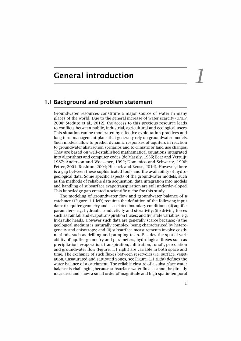
The modeling of groundwater flow and groundwater balance of acatchment (Figure. 1.1 left) requires the definition of the following inputdata: (i) aquifer geometry and associated boundary conditions; (ii) aquiferparameters, e.g. hydraulic conductivity and storativity; (iii) driving forcessuch as rainfall and evapotranspiration fluxes; and (iv) state variables, e.g.hydraulic heads. However such data are generally scarce because: (i) thegeological medium is naturally complex, being characterized by hetero-geneity and anisotropy; and (ii) subsurface measurements involve costlymethods such as drilling and pumping tests. Besides the spatial vari-ability of aquifer geometry and parameters, hydrological fluxes such asprecipitation, evaporation, transpiration, infiltration, runoff, percolationand groundwater flow (Figure. 1.1 right) are variable in both space andtime. The exchange of such fluxes between reservoirs (i.e. surface, veget-ation, unsaturated and saturated zones, see Figure. 1.1 right) defines thewater balance of a catchment. The reliable closure of a subsurface waterbalance is challenging because subsurface water fluxes cannot be directlymeasured and show a small order of magnitude and high spatio-temporal
1

1. General introduction
variability. This is particularly evident in water limited environments(Newman et al., 2005; Parsons and Abrahams, 2009), i.e. areas wherepotential evapotranspiration (PET ) is much larger than rainfall (RF ). Insuch environments, groundwater fluxes are generally small and grossrecharge (Rg) cannot be reliably determined by subtracting ET fromRF , since unavoidable small errors in the two lead to high inaccuracy ofRg (Hendricks et al., 2003; Lubczynski, 2011). Due to the difficulties inassessing the groundwater recharge, a common groundwater modelingpractice is to apply estimates of Rg a-posteriori during model calibra-tion, which often lead to bias in parameter estimation and erroneousgroundwater balances.
Figure 1.1: Left: definition of a catchment, showing boundaries, hy-drological fluxes and land use (modified after www.ogwa-hydrog.ca).Right: main surface and subsurface water fluxes (modified after www.sperchemical.com/water.html)
Sustainability of groundwater resources is controlled by the netgroundwater recharge (Sophocleous, 2005; Scanlon et al., 2006), definedby Rn = Rg−Exfg −ETg in which Exfg is groundwater exfiltration andETg is groundwater evapotranspiration. A source of bias in the assess-ment of Rn is not only uncertainty of evaluation of Rg but also typicalunderestimation, or even disregarding, of Exfg and ETg (Lubczynski,2000, 2009, 2011; Hassan et al., 2014), which leads to the overestimationof Rn. Exfg is the process of groundwater discharge in drainage areas,such as valleys, where the groundwater table intersects the topography,resulting in an interconnection between surface water and groundwater.Due to the complexity of exchange of water in such areas, Exfg is typic-ally simplified or disregarded in models despite its importance (Batelaanet al., 2003; Batelaan and De Smedt, 2004; Brunner et al., 2010). ETgis the ET component that refers to the process of groundwater uptakeby plant roots and by direct evaporation from water table or its capil-lary fringe (Lubczynski, 2009), representing an important componentof water balances particularly in water limited environments (Nichols,1994; Banta, 2000; Lubczynski, 2000; DeMeo et al., 2003; Loheide et al.,2005; Lubczynski and Gurwin, 2005; Naumburg et al., 2005; Shah et al.,2007; Sanderson and Cooper, 2008; Scott et al., 2008; Miller et al., 2010;Newman et al., 2010; Lubczynski, 2011; Orellana et al., 2012). The separa-
2

1.2. Research objectives
tion of subsurface ET into saturated and unsaturated zones componentsis referred as sourcing. As ET represents two physically different pro-cesses, evaporation (E) and transpiration (T ), each with different spatialand temporal characteristics, hydrological models need to account thesetwo processes separately (Guan and Wilson, 2009; Yang, 2015). There-fore, not only the sourcing but also the partitioning of ET into T andE should be implemented into hydrological models, by considering thefollowing subsurface ET components: unsaturated zone evaporation(Eu), groundwater evaporation (Eg), unsaturated zone transpiration (Tu)and groundwater transpiration (Tg) (Lubczynski, 2011). As recent studiesfocused on the assessment of these components individually (e.g. Shahet al., 2007; Balugani et al., 2014; Reyes-Acosta, 2015), such research cre-ated an opportunity to generate tools to integrate these fluxes separatelyin coupled hydrological models, allowing this way to retrieve a detailedand complete water balance at the catchment scale.
1.2 Research objectives
Groundwater model uncertainties are typically related to unknown spa-tial distribution of aquifer parameters and unknown spatio-temporaldistribution of driving forces, which lead to inaccurate or incorrect con-ceptual models. Moreover, the multiplicity of combinations betweenparameters and input fluxes results in non-uniqueness of groundwatermodel solutions. As a result, groundwater models are often unreliableand present limited forecasting capability.
To contribute to the constraining of groundwater models and reduc-tion of their uncertainties, the following two main objectives and relatedspecific objectives are proposed:
I. Spatial acquisition of subsurface parameters to contribute to thedesign of hydrological conceptual models:
1. Spatial subsurface parameterization of the hydrogeological me-dium using non-invasive techniques such as hydrogeophysics andremote sensing;
2. Design of conceptual models integrating hydrogeophysical andremote sensing data by using tools such as statistical modeling.
II. Spatio-temporal modeling of subsurface water fluxes and computingof detailed water balances at the catchment scale:
1. Development of a distributed lumped-parameter surface and soilzone model (MARMITES) and its coupling with the numericalgroundwater flow model MODFLOW to assess spatio-temporallythe subsurface water fluxes;
2. Computing of high-resolution, spatio-temporal water balanceat the catchment scale that incorporates the novel option ofpartitioning and sourcing of subsurface evapotranspiration.
3

1. General introduction
The proposed approach imposes additional constraints on groundwa-ter model calibration by providing a better spatial and temporal coverageof input data (subsurface parameters and fluxes) and by making possiblethe implementation of multi-criteria calibration on independent statevariables (e.g. surface runoff, soil moisture, hydraulic heads) belongingto the components of the coupled models (i.e. surface, unsaturated andsaturated zones). Non-uniqueness of model solution is expected to bereduced by computing more realistic boundary conditions, in particularnet groundwater recharge, through the implementation of a new model-ing option of partitioning and sourcing of subsurface evapotranspirationin the coupled MARMITES-MODFLOW model. Uncertainties in modeling,typically quantified using mathematical techniques during model calib-ration and automatic parameter optimization (Hill and Tiedeman, 2006;Doherty, 2015), are not presented hereafter because of a different focusof this study.
1.3 Proposed methodology
1.3.1 Spatial acquisition of aquifer parameters
Invasive measurements can be efficiently complemented by non-invasivehydrogeophysical and remote sensing methods which are time and costeffective. They succeed in covering large areas of land in a cheaper andquicker way than the invasive field sampling techniques. Hydrogeophys-ics provides methods of subsurface data acquisition to identify rockproperties and heterogeneities related with the presence of groundwa-ter (Rubin and Hubbard, 2005; Kirsch, 2009; Binley et al., 2015). Eachhydrogeophysical method has its own characteristics and capability withrespect to aquifer characterization, so the selection of the appropri-ate one must be done as a function of the objectives of a survey andgeological settings. Geoelectrical and electromagnetic methods havebeen widely used to retrieve hydrogeological structures and aquiferparameters using empirical, area-specific relationships. The magneticresonance soundings (MRS) method has definite advantage for quantitat-ive groundwater assessment in comparison to other hydrogeophysicalmethods because of its most direct relation to in-situ subsurface wa-ter. The complementarity and joint use of hydrogeophysical methodsconstitutes the most powerful tool to characterize aquifers. Howeverthese methods are generally restricted to local scale, either in 1D or 2D.Therefore techniques of interpolation and/or extrapolation of data at thecatchment scale are required to integrate hydrogeophysical informationinto hydrogeological models. Remote sensing, together with statisticaland geostatistical interpolation methods, are particularly adequate forthat purpose. Hydrological information can be extracted from remotesensing images and correlated to hydrogeological and hydrogeophysicaldata, allowing to extend the data to the image coverage. Although someremote sensing methods can also retrieve quantification of water fluxes,
4
1.4. Thesis outline
this component was not included in this thesis.
1.3.2 Spatio-temporal modeling and assessment of subsurfacewater fluxes
The transient calibration of hydrological models requires time series ofdriving forces and state variables. Such data can be acquired throughmonitoring networks. Nowadays, automatic data acquisition systems areroutinely used to acquire such data, thanks to the low cost and advance-ment of electronic devices, i.e. sensors and loggers. Such monitoringnetworks allow to register at high temporal frequency and high spatialresolution the meteorological forces (e.g. precipitation, wind speed, airtemperature, solar radiation) that control the hydrological dynamic ofa catchment, as well as the related state variables (e.g. soil moisture,hydraulic heads, stream flow). The data acquisition can be designedusing several monitoring stations located at key points of the catchment,e.g. recharge/discharge areas, allowing to register the spatio-temporalvariability of the driving forces and the responses of the hydrologicalsystem. Such data are critical to provide reliable and realistic input tohydrological models (Holländer et al., 2015).
In this study, the conversion of meteorological data into boundaryfluxes is proposed to be implemented through the newly developedMARMITES model. This model integrates the surface and soil zonesand computes spatio-temporally the partitioning of rainfall into evap-oration, transpiration, infiltration, runoff, percolation and groundwaterrecharge. The MARMITES model is two-way coupled with the groundwa-ter MODFLOW-NWT model, i.e. the two models can exchange boundaryconditions among themselves. Such coupling allows to integrate the in-teraction between surface and subsurface fluxes, particularly dynamic indrainage areas where groundwater and surface water are interconnected.
Although many models are available, it was opted in this study todevelop the new surface and soil zones MARMITES model to implementthe novel options of partitioning and sourcing of the evapotranspira-tion fluxes. Partitioning refers to the separation of the evapotranspira-tion (ET ) into the evaporation and transpiration components while thesourcing corresponds to the separation of ET into unsaturated zoneand groundwater evapotranspiration. The partitioning and sourcing ofevapotranspiration fluxes is relevant not only to improve the reliability ofmodels and water balances but also to understand the role of vegetationand soil processes in the water cycle and to make reliable predictionscenarios of climate and land use changes.
1.4 Thesis outline
Chapters 2, 3 and 4 present methodologies based on hydrogeophysics,remote sensing and geostatistics to contribute to the design of hydro-geological conceptual model. Chapter 5 presents the development of
5

1. General introduction
the coupled MARMITES-MODFLOW model of surface, unsaturated andsaturated zones that computes spatio-temporally the water fluxes atthe catchment scale and integrates the sourcing and partitioning of theevapotranspiration. The coupled model capabilities are demonstratedthrough a case study. Finally, Chapter 6 presents the integration ofMRS-based hydrogeophysics into the coupled model.
To implement and test the proposed methodologies, we selected 4study areas located in the Iberian peninsula, all of them in semi-aridclimate. Two study areas, the Pisões catchment (Alentejo, Portugal,Chapter 2) and Sardón catchment (Salamanca, Spain, Chapters 4 and 5and Appendix A) are located in hard rock aquifer regions. Hard rockscover large geographical areas and often constitute the only source ofwater supply for population, livestock and agriculture. As hard rocksare characterized by large spatial heterogeneity and low storage, themodeling of aquifer in such environment is a challenge. The thirdstudy area corresponds to a coastal aquifer located in Algarve (SouthPortugal, Chapter 3), in a complex hydrogeological settings. Finally thelast study area, the Carrizal catchment (Salamanca, Spain, Chapter 6),is characterized by Cenozoic, fluvial deposits that support a multilayer,porous aquifer.
In Appendix A an article entitled "Using Ground Penetrating Radarto investigate the water table depth in weathered granites - Sardón casestudy, Spain" by Mahmoudzadeh et al. (2012) is presented. This article isco-authored by the author of this thesis. It presents a GPR application toretrieve the groundwater table depth in weathered granites in the Sardónstudy area, referred in Chapters 4 and 5. This article was not includedas a chapter of the thesis because the main GPR technique applied inthis study is not the primary expertise of the author of this thesis.
1.4.1 Chapter 2
This chapter introduces a method based on invasive sampling, surfacegeophysics, remote sensing and geostatistics to predict the clayey topsoilthickness of a small catchment in Portugal. The approach is based on con-tinuous, non-invasive electromagnetic (frequency domain) measurementsalong transects in order to capture the geomorphological dependenceof the topsoil thickness. Based on statistical correlation and calibrationwith the invasive measurements, geophysical results are extrapolatedusing geostatistical methods and remote sensing images as auxiliarydata.
1.4.2 Chapter 3
The objective of this chapter was to retrieve the structure and geometryof a coastal aquifer and to upgrade the current hydrogeological concep-tual model. The methodology was based on hydrogeophysical methodssuch as 2D electric resistivity tomography (ERT), 2D frequency domainelectromagnetic (FDEM) and 1D time-domain electromagnetic (TDEM)
6

1.4. Thesis outline
applied along transects transversal and longitudinal with respect to theaquifer. The hydrogeophysical interpretation was supported with auxili-ary information such as regional piezometric map and borehole litholo-gical logs, as well as offshore data. The hydrogeophysical methods wereeffective in detecting the position of the freshwater-saltwater interfaceand allowed redefining the boundaries and 3D structure of the coastalaquifer. The new redefined hydrogeological conceptual model supportsthe explanation of the location of the inter- and subtidal fresh ground-water discharge and constitute the basis of variable-density groundwaterflow numerical model.
1.4.3 Chapter 4
In this chapter, a methodology of data acquisition for hydrogeologicalconceptual models, particularly suitable for data scarce areas, is presen-ted. It involves remote sensing and non-invasive hydrogeophysical meth-ods supported by hydrogeological field data acquisition to derive thehydrogeological conceptual model of a hard rock aquifer. Instead ofinterpolation or extrapolation methods of the acquired data, a downwardapproach is applied. This approach consists of analyzing patterns indata observed at the catchment scale to retrieve the hydrological char-acteristics of the catchment. The remote sensing analysis allowed todefine the main hydrogeological features that were locally characterizedand parameterized using several hydrogeophysical methods such as2D ground penetrating radar (GPR), 2D electric resistivity tomography(ERT), 2D frequency domain electromagnetic and 1D magnetic resonancesoundings (MRS). After verification and calibration using drilling andslug tests, hydrogeophysical results of each hydrogeological featureswere compiled and integrated into a hydrogeological conceptual model.
1.4.4 Chapter 5
A coupled model composed of the new land surface and soil zone MAR-MITES model and of the USGS groundwater MODFLOW-NWT model ispresented to demonstrate model-based partitioning and sourcing ofevapotranspiration (ET ) as part of spatio-temporal water balancing atthe catchment scale. The partitioning of ET involves its separationinto evaporation and transpiration while the sourcing of evaporationand transpiration involves separation of each of the two fluxes intosoil and saturated zone components. The capability of the MARMITES-MODFLOW coupled model to simulate complex hydrological systems isdemonstrated by its application to a small catchment characterized by asemi-arid climate with rainfall ∼500 mm.y−1, granitic bedrock, shallowgroundwater and sparse oak woodland.
7

1. General introduction
1.4.5 Chapter 6
This chapter presents the integration of hydrogeophysical, magnetic res-onance soundings (MRS) method of data acquisition into the MARMITES-MODFLOW model. The MRS method provides quantitative hydrogeo-logical information on hydrostratigraphy and hydraulic parameters ofsubsurface, e.g. flow and storage property of aquifers. The originalintegration method is based on the optimization of the MRS estimates ofaquifer hydraulic parameters through hydrologic model calibration. TheMRS integration with hydrologic model was carried out by introducingmultipliers of specific yield and transmissivity/hydraulic conductivitythat were optimized during transient model calibration using time-seriespiezometric observation points.
8

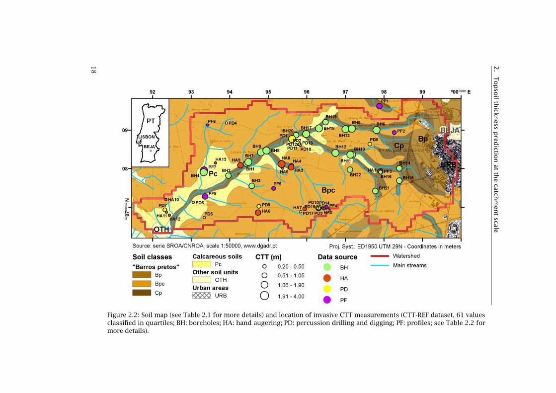
Geonics™ EM-31 instrument on plowed fields of the Pisões catchment (Beja,Alentejo, Portugal).


2Topsoil thickness prediction atthe catchment scale byintegration of invasive sampling,surface geophysics, remotesensing and statistical modeling
2.1 Introduction
Distributed hydrological models have a wide range of applications inagronomy, hydrology and hydrogeology, e.g. in crop management, runoffand flood studies, land-use and climate change impacts, and assessmentof groundwater resources renewability (Finch, 1998; Lubczynski andGurwin, 2005; Rushton et al., 2006; Batelaan and de Smedt, 2007). Suchmodels typically partition rainfall into: evapotranspiration, soil moisturestorage, groundwater recharge and surface runoff. This partitioninglargely depends not only on the hydrological conditions, but also onthe pedo-geological conditions. Topsoil thickness, in conjunction withsoil hydraulic properties, controls the water holding capacity and istherefore a critical parameter in the assessment of groundwater recharge.The spatial assessment of topsoil thickness is difficult due to its highspatial heterogeneity, which is controlled by several factors such asclimate, geomorphology and parent material. Invasive data acquisitiontechniques such as drilling or trench excavations are labor-intensive,costly and involve extensive fieldwork sampling and laboratory analysis.They can be efficiently complemented by non-invasive geophysical andremote sensing (RS) methods which are time and cost effective, i.e. theysucceed in covering large areas of land cheaper and quicker than the soilsampling techniques.
This chapter is based on: Topsoil thickness prediction at the catchment scale byintegration of invasive sampling, surface geophysics, remote sensing and statisticalmodeling. Francés, A. P., and M. W. Lubczynski (2011), Journal of Hydrology, 405, 31-47
11

2. Topsoil thickness prediction at the catchment scale
Geophysics, as an indirect method, measures one physical propertyof the subsurface that has to be converted into a parameter or variableof interest. For instance, electrical conductivity per se is of little inform-ation in a hydrological sense if it is not related to soil moisture or soilsalinity, i.e. a physical property that affects the soil. Its conversion can bedeterministic or statistical (Corwin and Lesch, 2003). The deterministicapproach assumes an a-priori knowledge of the mechanism from thestudied processes, and its mathematical formulation through theoreticalor empirical models. However, it often requires several parameters thatare not available and/or expensive to acquire. The statistical approach,although site-specific, is more flexible. The statistical models are built bymeasuring target soil variables at a limited number of sampling points.Several authors (Knotters et al., 1995; Odeh et al., 1995; Bourennaneet al., 2000; Bishop and McBratney, 2001; Triantafilis et al., 2001a,b;Bourennane and King, 2003; Kuriakose et al., 2009) have applied thestatistical approach to predict the spatial distribution of soil variablesby use of auxiliary variables such as geophysical measurements and RSinformation. They have used and sometimes compared several statisticalmethods such as simple linear regression (LR), multiple linear regression(MLR), variance analysis (ANOVA), covariance analysis (ANOCOVA) andkriging techniques, such as ordinary kriging (OK), cokriging, universalkriging (UK) and kriging with external drift (KED). These statistical andgeostatistical techniques are derived from the general universal modelof spatial variation as defined by Matheron (as cited in Hengl, 2009),which is also called the geostatistical mixed linear model (MLM) by Leschand Corwin (2008). For any given dataset, the selection of an adequateprediction model derived from the MLM approach cannot be exclusivelybased on the model performance and goodness of fit. The selection mustbe primarily made by the verification of the model assumptions. In thisstudy we applied the guidelines of Lesch and Corwin (2008), which ex-plained the connection between the LR model and the MLM, reviewed theunderlying assumptions and presented statistical diagnostic tools. Wealso followed the methodology of Hengl (2009) who developed a decisionchart, based on the sequential verification of the model assumptions, toguide in selecting an appropriate prediction model.
The soil apparent electrical conductivity (ECa) retrieved by geophys-ical techniques, such as electrical resistivity (ER) or electromagnetic (EM)methods, has been used in environmental sciences to efficiently charac-terize the subsurface (Corwin and Lesch, 2005b). ECa depends on thecombination of several properties of the subsurface such as electricalconductivity of the soil aqueous solution, volumetric water content, soiltexture, mineralogy and temperature (Corwin and Lesch, 2003; Friedman,2005). Depending on the site-specific properties and the land manage-ment in agricultural areas, generally one or two of these properties (e.g.salinity, clay content, soil moisture, etc.) contribute more than the othersin the measured ECa value. This may even lead to different ECa values intwo adjacent plots of the same soil type which have different agriculturalpractices. This non-uniqueness in the relationship between the ECa and
12

2.1. Introduction
the soil properties makes the interpretation of ECa data difficult andgenerally limits its usability at the plot scale where subsurface conditionsare relatively homogeneous.
The RS proved to be an efficient complement to the invasive methodsand the geophysical surveys. RS allows integration within the spatialheterogeneity into the modeling of the relationship between the ECaand soil properties. Bishop and McBratney (2001) compared severalprediction methods to map the soil cation exchange capacity (CEC) at theplot scale based on a combination of ECa measured by ER method, baresoil color obtained by RS information (LANDSAT TM imagery and aerialphotographs), terrain parameters and crop yield data. They found thatthe CEC was better estimated with the statistical models that integratedeither the bare soil information, which was obtained from color aerialphotographs, or the ECa. Triantafilis et al. (2001a) predicted the claycontent at the field scale by testing several spatial prediction models.The spatial prediction models that integrated auxiliary variables suchas ECa from Geonics™ EM-31 and EM-38 survey and RS color bands ofaerial photographs proved to be more accurate.
The approach of combining geophysical ECa with RS data and statist-ical modeling was tested at a larger scale by several authors. For mappingclay content at a landscape scale, Weller et al. (2007) applied a nearestneighbor correction to the ECa data measured with EM-38 in agriculturalfields. This method reduced the variance of the ECa data by more than50% and improved the coefficient of determination (R2) from 0.66 (nocorrection) to 0.85. Triantafilis and Lesch (2005) mapped the average claycontent for a 0-7 m depth range at the catchment scale (∼60 km2) usingthe ECa data measured with EM-34 and EM-38 instruments. They useda fuzzy k-means method to classify the ECa data into physiographicand hydrological units. In each unit, a relationship between the ECasignal measured by the EM-34 and the EM-38 and the first-order trendsurface component was applied to predict the averaged clay content.They concluded that although the method was useful to determine a soilsampling scheme, it did not result in an improvement in the relationshipbetween ECa and the averaged clay content. They recommended theincorporation of remotely sensed information (e.g. gamma radiometric,LANDSAT, RADARSAT, etc.) into the classification process.
The focus of this study, i.e. the spatial variability of topsoil thickness,has already been investigated by several authors at the plot scale inrelatively homogeneous areas characterized by low relief and low slopes.In all prior cases, a high contrast of ECa was observed between overlayingsoil horizons due to texture differences. Doolittle et al. (1994) found ahigh correlation between the depth to claypan (d) and the ECa measuredby EM-38 using an exponential regression model d = ne(mECa), where mand n were the model constants. Sudduth et al. (2003) obtained goodresults in claypan soils using a linear regression between the topsoilthickness and the inverse of the ECa. Brus et al. (1992) predicted theboulder clay depth beneath a sand cover using ECa values measuredby EM-38 and EM-31. They used regression analysis to fit an empirical
13

2. Topsoil thickness prediction at the catchment scale
exponential model and a physical spherical model, concluding that theuse of ECa to predict topsoil thickness was not very appropriate due tothe fact that the ECa was affected by spatial variation in the soil moisture.They improved the relationship by integrating land-use information thataccounted for soil moisture variation. In addition, they recommendedthe integration of RS with ECa data into the modeling process in order tobetter account for the spatial variation of soil variables and parameters.These suggestions were followed by Bourennane and King (2003) whopredicted satisfactorily the topsoil thickness at the plot scale by usingECa and the slope gradient. Kuriakose et al. (2009) implemented theprevious methodologies on a larger scale, i.e. to a small catchment(∼9 km2), and predicted the soil depth using an extensive dataset ofinvasive measurements (276 values). They applied several statisticaland geostatistical methods that integrated topographic variables derivedfrom a digital elevation model (DEM) and land use map information.
The objective of this study was to predict the topsoil thickness atthe catchment scale and to use this prediction as input in a hydrologicaldistributed model in further studies. We developed a novel data acquisi-tion and data-integration method applicable at the catchment scale thatlimited the number of invasive field observations. The proposed methodinvolved: (i) invasive sampling (augering and drilling); (ii) surface geo-physics using EM-31; (iii) RS imagery (high resolution QuickBird image,aerial orthophotos and ASTER GDEM) processing; and (iv) MLM approachand model diagnostic.
We applied the proposed method in the Pisões catchment (19 km2)of the Alentejo province in Portugal, to predict the spatial distributionof the clayey topsoil thickness (CTT). The CTT was recognized as amajor controlling factor in the hydrological processes. It was thereforecritical for an adequate parameterization of the distributed unsaturatedmodel that was developed in order to improve the groundwater resourceassessment (Chapter 5, Francés and Lubczynski, 2015).
2.2 Material and methods
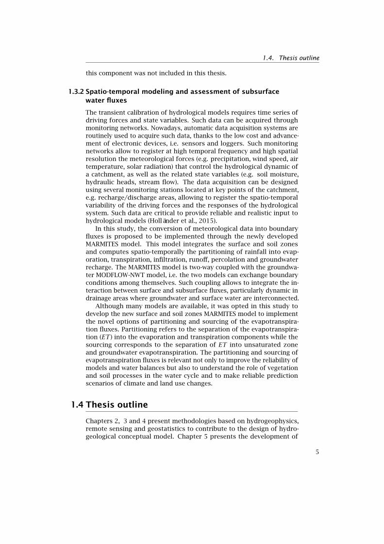
The general methodology of the CTT spatial prediction combines invasivesampling, surface geophysics, RS and the MLM approach and is presentedin the flowchart in Figure 2.1. In step 1, we compiled a preliminarydataset of invasive CTT measurements based on previous studies. Insteps 2 and 3, we analyzed and processed the RS imagery to obtainthe soil classification and terrain parameters. In step 4, following theinformation acquired in steps 1-3, we designed the sampling scheme ofthe surface-geophysics (EM-31 ECa measurements) and complementaryCTT invasive measurements that, together with the compiled CTT data ofstep 1, constituted the CTT reference dataset (CTT-REF). We establisheda calibration dataset (CTT-CAL) composed of co-located pair-points ofinvasive CTT measurements and corresponding ECa data. In step 5, weapplied several calibration models, based on the MLM approach and the
14

2.2. Material and methods
integration of auxiliary spatial information (soil classification of step2 and terrain parameters of step 3), to convert the ECa data into CTTto obtain the CTT-EC dataset. In step 6a, we predicted the CTT at thecatchment scale by using the MLM approach and the CTT-EC dataset(CTT-ECpred raster). In step 6b, we performed a similar procedure toobtain the CTT-REFpred raster but by using exclusively the invasive CTTmeasurements (i.e. CTT-REF). The objective for performing these twopredictions was to assess the effectiveness of the geophysical data asa substitute for invasive observations. Finally, in step 7, we assessedthe quality of the prediction models by computing the mean error (ME),the mean absolute error (MAE) and the root mean square error (RMSE)between the predicted (CTT-ECpred and CTT-REFpred rasters) and theobserved (CTT-REF) dataset.
All the spatial data acquired from the field and from RS imagery(steps 1 to 4) were converted into the same projected coordinate system(ED50-UTM zone 29N). To retrieve the positions of the invasive CTT meas-urements, the geophysical data points and several geodetic benchmarks,we used a standard GPS receiver (GARMIN GPSMAP 60C). To convertthe coordinates we utilized the seven transformation parameters of theBursa-Wolf method. We obtained a horizontal positional accuracy of∼2.5 m, which was satisfactory considering the scale of the CTT spatialvariation.
15
2. Topsoil thickness prediction at the catchment scale
Figure 2.1: Flowchart of the methodology used to predict the CTT at thecatchment scale.
16

2.2. Material and methods
2.2.1 Study area
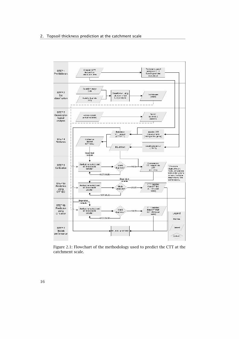
The Pisões catchment (∼19 km2) is located in the Alentejo region (Por-tugal), west of Beja city (Figure 2.2). The topography is smooth, withgentle slopes and flat surfaces. The catchment boundaries correspond tothe basin water divides. The perennial Ribeira da Chamine stream drainsa phreatic aquifer, flowing to the south-west towards the catchmentoutlet. The catchment water table follows the topography, becomingdeeper in the hill tops and more shallow within the drainage areas. Theland use is mainly characterized by rainfed agriculture (wheat and olivegroves), although in the last decade the practice of irrigating crops (dripirrigation for olive groves and sprinkler pivot for corn and beetrootcrops) has become more common. These practices, combined with thehigh evapotranspiration rate, have provoked an increase in soil salinity.
The geology of the study area is composed of gabbros and diorites(Oliveira, 1992). The chemical weathering of the gabbro-dioritic rockshas resulted in the formation of clay minerals, mainly montmorillonite(Vieira e Silva, 1991). The main soil classes (Cp, Bp and Bpc, see Figure 2.2and Table 2.1) belong to the so-called Barros Pretos unit (Cardoso, 1965).The high concentration of swelling clay in the topsoil provokes thedevelopment of wide and deep cracking systems during dry seasons.The soil profiles consist of a clayey topsoil (horizons AB) overlyinga weathered parent rock material (horizon C) that can be carbonate-rich (Table 2.1). The AB horizon is thicker along the drainage areaof the catchment (Cp class) than in the Bp and Bpc classes. Alongthe steep slopes, carbonate soils (Pc class, so-called calcrete) outcroppredominantly (Figure 2.2). They are characterized by a thinner ABhorizon and a lighter color than the other soil classes (Cp, Bpc and Bp).
17
2.
Topso
ilth
ickness
pred
iction
atth
ecatch
men
tscale
Figure 2.2: Soil map (see Table 2.1 for more details) and location of invasive CTT measurements (CTT-REF dataset, 61 valuesclassified in quartiles; BH: boreholes; HA: hand augering; PD: percussion drilling and digging; PF: profiles; see Table 2.2 formore details).
18
2.2
.M
ateria
land
meth
ods
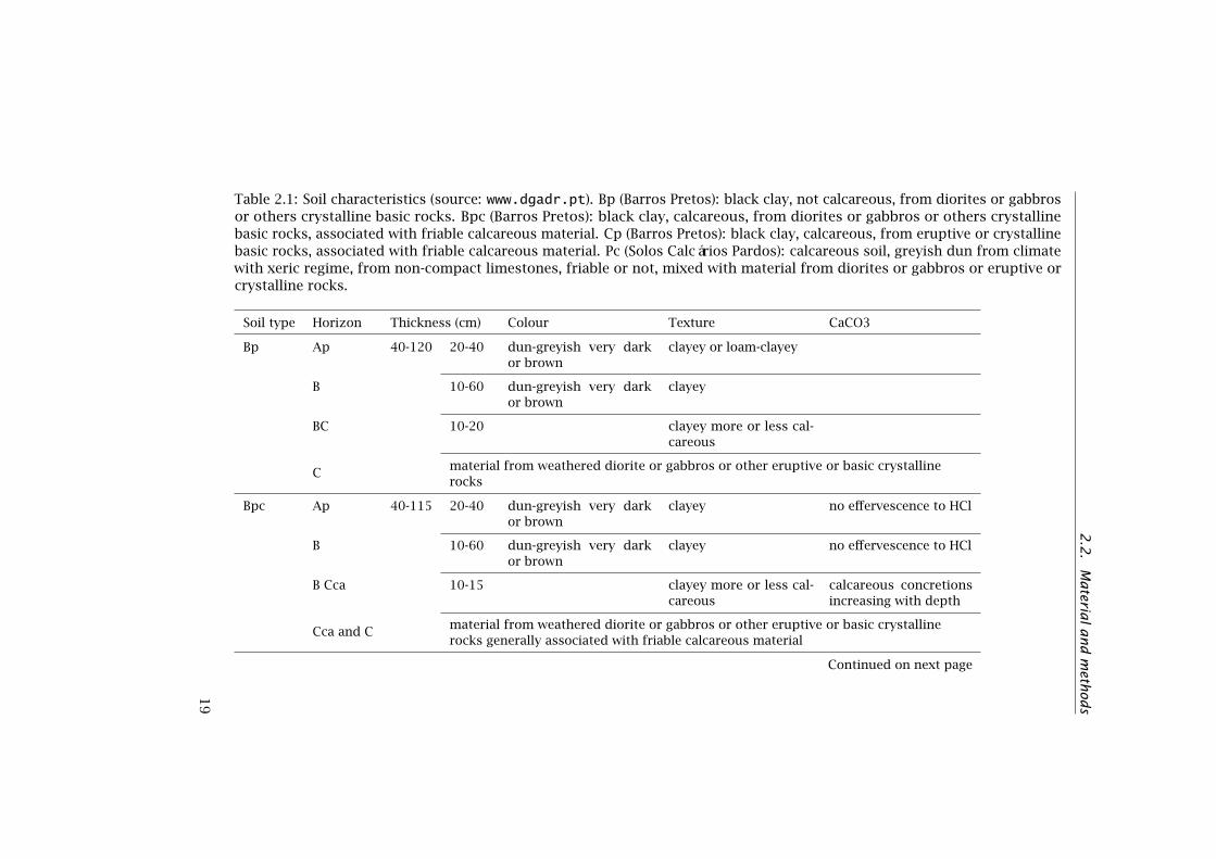
Table 2.1: Soil characteristics (source: www.dgadr.pt). Bp (Barros Pretos): black clay, not calcareous, from diorites or gabbrosor others crystalline basic rocks. Bpc (Barros Pretos): black clay, calcareous, from diorites or gabbros or others crystallinebasic rocks, associated with friable calcareous material. Cp (Barros Pretos): black clay, calcareous, from eruptive or crystallinebasic rocks, associated with friable calcareous material. Pc (Solos Calcários Pardos): calcareous soil, greyish dun from climatewith xeric regime, from non-compact limestones, friable or not, mixed with material from diorites or gabbros or eruptive orcrystalline rocks.
Soil type Horizon Thickness (cm) Colour Texture CaCO3
Bp Ap 40-120 20-40 dun-greyish very darkor brown
clayey or loam-clayey
B 10-60 dun-greyish very darkor brown
clayey
BC 10-20 clayey more or less cal-careous
C material from weathered diorite or gabbros or other eruptive or basic crystallinerocks
Bpc Ap 40-115 20-40 dun-greyish very darkor brown
clayey no effervescence to HCl
B 10-60 dun-greyish very darkor brown
clayey no effervescence to HCl
B Cca 10-15 clayey more or less cal-careous
calcareous concretionsincreasing with depth
Cca and C material from weathered diorite or gabbros or other eruptive or basic crystallinerocks generally associated with friable calcareous material
Continued on next page
19

2.
Topso
ilth
ickness
pred
iction
atth
ecatch
men
tscale
– continued from previous page
Soil type Horizon Thickness (cm) Colour Texture CaCO3
Cp Ap 80-165 25-40 dun-greyish dark to verydark or gray very darkor brown
clayey no effervescence to HCl
B 45->100
dun-greyish dark to verydark or gray very darkor brown
clayey calcareous concretionsincreasing with depth
B Cca 10-25 mixing of B horizon, C horizon and friable calcareous material and/orcalcareous concretions
Cca and C material from weathered eruptive or basic crystalline rocks associated with friablecalcareous material
Pc Ap 20-40 20-40 dun, clear dun,yellowish-dun or dun-greyish
loam-clayey to clayey,calcareous
strong effervescence toHCl
Cca and C material from the weathering of non-compact limestones, friable or not, mixedwith material from diorites or gabbros or eruptive or crystalline rocks
20

2.2. Material and methods
2.2.2 Invasive sampling
We compiled a reference dataset of 61 invasive CTT measurements (CTT-REF) derived from several data sources (Figure 2.2 and Table 2.2). Wealso collected soil samples to characterize the soil horizons properties(see below). The CTT-REF was composed of: (i) 39 data points compiledfrom previous work (data obtained from borehole drilling reports, handaugering and profile analysis in pitches); and (ii) 22 new invasive CTTmeasurements made during fieldwork in September 2007 and Septem-ber 2009. The locations of the new CTT measurements were selectedusing purposive sampling in order to obtain an equal coverage of thegeomorphologic features of the catchment and be positioned along thegeophysical transects. The soil sampling was difficult due to the hard-ness of the clayey topsoil during dry season and softness in wet season.In zones where the topsoil was thin (∼0.5 m), we made observations andsampling using hand augering or digging with appropriate tools (shovels,digging hoes and pick axes). In thicker clayey soils, we used a gasolinepowered COBRA percussion hammer. Although this technique was time-consuming (∼2 h per core of 2 m depth), it allowed us to collect soilsamples at different depths (up to 2.5 m) and to measure the CTT. Onlyone drilling profile was performed in the drainage area (Cp soil class), atlocation PD1 (Figure 2.2). This profile did not reach the C horizon due tothe drilling equipment’s limited depth of penetration. No samples weretaken from the Bp class since it was very similar to the Bpc class andonly present on a small area of the NE of the catchment (Figure 2.2).
Table 2.2: Reference dataset of invasive CTT measurements (CTT-REFdataset, 61 values).
Data Description Number Collector Period
source of data
BH borehole drillingreports
22 Severalcompanies
1960-2000
HA hand augering 9 Cortez (2004) 09/2003
4 This study 09/2009
PD shallow percussiondrilling/digging
18 This study 09/2007
PF profiles analysis inpitches
8 Paralta (2009) 05-07/2005
21

2. Topsoil thickness prediction at the catchment scale
2.2.3 Soil analysis
We characterized the AB and C soil horizons based on soil texture de-termination, laboratory mineral spectra analysis and dielectric propertymeasurements. Such characterization was necessary to interpret thesurface geophysical measurements. The soil texture was determinedby Paralta (2009) for each sub-horizon of the 8 soil profiles of the PFcategory (Table 2.2 and Figure 2.2). In total, 25 samples were collectedand analyzed (23 from horizon AB and 2 from horizon C). For eachprofile, we computed the average clay content in the horizon AB (theaverage was weighted by the thickness of the 23 sub-horizons). Weperformed mineral recognition of the soil horizons by means of mineralspectra analysis of 32 samples in the PD dataset (Table 2.2) taken at 11locations (PD1 to PD10 and PD13, Figure 2.2). 15 samples were fromthe AB horizon and 17 from the C horizon. Finally, we measured theapparent soil electrical conductivity of discrete, homogeneous soil ho-rizons (ECs ) to check the consistency with the surface geophysics ECa,since the latter corresponds to a bulk measurement of the soil horizonsECs above the depth of penetration of the geophysical instrument. Wemeasured the real (ε′r ) and imaginary (ε′′r ) dimensionless components ofthe soil complex dielectric permittivity with a portable Stevens HydraProbe (Seyfried and Murdock, 2004; Seyfried and Grant, 2007) on theAB and C horizons at 10 vertical soil profiles (locations PD1 to PD10,Figure 2.2). ECs (S/m) is related to ε′′r as following:
ECs = ε0ε′′r f2π (2.1)
where ε0 is the free space permittivity (8.854×10⁻¹² F.m−1) and f is themeasurement frequency (50 MHz). A correction for temperature effectwas considered as suggested by Seyfried and Grant (2007) in order toobtain standardized values of ECs at 25°C. The areas with a ratio ofε′′r /ε′r>2 were identified as affected by soil salinity (Seyfried et al., 2005).
2.2.4 Remote Sensing
2.2.4.1 Soil classification
The general purpose of any soil classification is to identify groups withone or several homogeneous properties. This advantageously reducesthe variability in relation to the whole population, while increasing theprecision of any prediction made. Each soil type class in Figure 2.2indicates a range of CTT, as shown in Table 2.1. The introduction of theseclasses in statistical modeling improves the relationship between the CTTand the explanatory variables (geophysical data and terrain parameters).However, in this study the only soil map available (Figure 2.2) was notapplicable because its scale (1:50 000) was too coarse for the requiredlevel of details. In addition, our field observations were in disagreementwith that map. We thus decided to perform our own soil classificationbased on field observation and on RS interpretation. At the end of
22

2.2. Material and methods
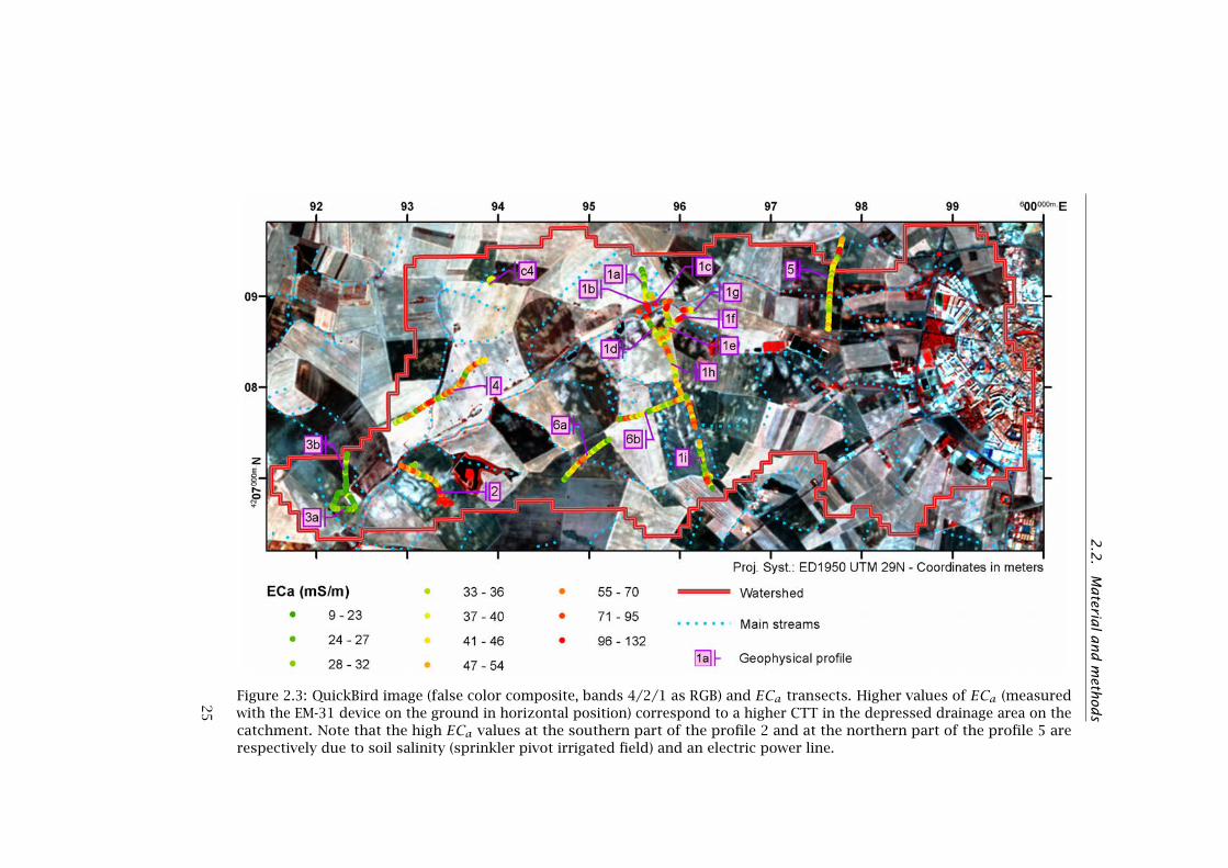
the dry season, the agricultural fields are bare and the color of thesurface is indicative of the dominant soil type. Although the whitishcalcrete outcrops can be visually identified among the darker clayey soils(Figure 2.3), the RS recognition of the soil types and its classification isadditionally complicated by the occurrence of dark and bright fields dueto the presence or the absence of dry crops and plowing. For example,a calcrete soil area in a dark field has a spectral signature similar to aclayey soil area in a bright field resulting in classification non-uniqueness.However, as the color intensity of the dark and bright fields variesthroughout the year and seasons due to crop rotation, the confusingeffect of dark and bright fields can be minimized by analyzing imagesacquired at different periods. In this study, we fused a multispectralQuickBird (QB) high resolution image from the 20th of September 2006at 11:40 (GMT) (Figure 2.3 and Table 2.3) and a 3 bands (RGB) aerialorthophoto (AO) of 0.5 m resolution, acquired in November 2004 bythe Instituto Geográfico Português (IGP). The fusion of the QB with AOimages was done according to the following procedure: (i) pre-processingusing a smoothing filter (9x9 pixels for QB; 11x11 for AO) to attenuatethe linear structures due to plowing; (ii) conversion of the wave lengthinto DN values; (iii) coordinates conversion and rectification; and (iv) thefusion of the two images at the QB resolution (QBAO image).
Table 2.3: Main characteristics of the QuickBird image, cloud-free, ac-quired the 20th of September 2006 at 11:40 (GMT). Acquisition time, closeto sun zenith, was convenient to minimize the shadows and influence ofsunray obliquity on the images color and brightness.
Sensorresolution
Dynamicrange
Spectral bandwidth (nm)
Band 1(blue)
Band 2(green)
Band 3(red)
Band 4(NIR)
2.4 mmultispectralat nadir
11 bits perpixel
450 to520
520 to600
630 to690
760 to900
Since the pixel-based approach was not suitable to classify the studyarea into calcrete (CALCR) and clayey (CLAY) soils due to the non-uniqueness of the spectral signature, we applied an object-orientedfuzzy-logic analysis (Benz et al., 2004) using the Definiens Developer7 software. This approach produces very good results for the cases inwhich the spectral based classification approach is causing confusionbetween classes due to their similar spectral characteristics. Some ex-amples are burned areas mapping Mitri and Gitas (2002) and land usemap production in complex mosaics of urban, forest and agriculturalareas (Al Fugara et al., 2009). The object-oriented fuzzy-logic analysisincorporates two main steps: segmentation and classification. The imageis first segmented into object primitives (groups of pixels that sharesimilar spectral signature) based on region-merging techniques. The
23

2. Topsoil thickness prediction at the catchment scale
merging, which starts with a one-pixel object, is iteratively processedwhile the heterogeneity between adjacent object primitives, which refersto gray tones and shapes, is less than a certain threshold. In the nextstep, the nearest neighbor (NN) classification and fuzzy logic are used toclassify the object primitives into real-word objects. To define the fea-ture space, the user first selects the spectral properties of the real-wordobjects. Second, the user collects training samples representative of thereal-word objects. The distance between the object primitives and thenearest real-word objects in the feature space is computed. Then, byusing fuzzy logic, this distance is converted into a membership valuethat varies between 1 (belong to the class) and 0 (does not belong tothe class). Each object primitives is then classified into the real-wordobjects to which the membership score is higher. We applied this meth-odology to obtain the soil classification using the fused QBAO image asfollowing: (i) multi-resolution segmentation based on the 7 bands (4 fromQB and 3 from AO); (ii) classification of the study area into dark fields(DF), bright fields (BF) and other land covers (vegetation, urban areasand water bodies) using training samples and standard NN method; and(iii) reclassification of DF and BF in CLAY and CALCR soil types: DFclay(dark), DFcalcr (intermediate), BFclay (intermediate) and BFcalcr (bright)using fuzzy logic and NN. Our target was to reach an overall accuracy(computed between the training samples and the final classification)higher than 95%.
24
2.2
.M
ateria
land
meth
ods
Figure 2.3: QuickBird image (false color composite, bands 4/2/1 as RGB) and ECa transects. Higher values of ECa (measuredwith the EM-31 device on the ground in horizontal position) correspond to a higher CTT in the depressed drainage area on thecatchment. Note that the high ECa values at the southern part of the profile 2 and at the northern part of the profile 5 arerespectively due to soil salinity (sprinkler pivot irrigated field) and an electric power line.
25

2. Topsoil thickness prediction at the catchment scale
2.2.4.2 Terrain parameters
The terrain geomorphology controls the intensity of erosion and depos-ition processes and influences soil formation and evolution. To studythe relationship between the CTT and the geomorphology, we computedseveral terrain parameters that summarize the terrain capacity to ac-cumulate or to transport sediments. We utilized the methodology andalgorithms presented in Hengl et al. (2003a) to derive the morphometricand hydrological terrain parameters. The morphometric terrain para-meter groups describe the morphology of the surface that controls thewater flow. They are computed by using elevation gradients between theactual cell and its 8 surrounding cells. We computed: (i) slope (SLOP);(ii) mean curvature (MEANC); (iii) vertical or profile curvature (PROFC);and (iv) plan curvature (PLANC). The hydrological (or flow accumulation-based) terrain parameter groups quantify flow intensity, accumulationpotential and erosion potential. They are computed using the upslopecontributing area per unit contour length draining through the cell andthe local slope angle. The parameters used in this study are: (i) topo-graphic wetness index (TWI); (ii) stream power index (SPI); and (iii) sedi-ment transport index (STI). We also computed the topographic positionindex (TPI) defined by Weiss (2001) using the algorithm of Jenness (2006).TPI is a quantitative representation of the elevation of the actual cell inrelation to the elevation of the surrounding cells (selected by a user-inputbuffer), which represents the erosion/accumulation capacity of the ter-rain. We derived the terrain parameters from the Global Digital ElevationModel (GDEM) of the Advanced Spaceborne Thermal Emission and Re-flection Radiometer (ASTER) satellite (www.gdem.aster.ersdac.or.jp).The ASTER stereoscopic capability using the near infrared spectral bandpermits the derivation of a DEM which has a spatial resolution of 15 m inthe horizontal plane, and a horizontal accuracy of 30 m at 95% confidenceand vertical accuracy of 20 m at 95% confidence. We verified the hori-zontal accuracy and confirmed the GDEM compatibility with the previousdataset (RS imagery and geophysics). The absolute vertical accuracy wasconsidered not relevant in this study if the image did not show distortion,i.e. if the relative error was spatially uniform. We compared the GDEMwith a digital terrain model (DTM) computed from a digital vectorialtopographic map (Portuguese cartographic institute IGeoE, sheet 521,SÃl’rie M888 Continente at scale 1:25 000, www.igeoe.pt) obtained bystereophotogrammetry on aerial images. The IGeoE-DTM was created astriangulated irregular network format using ArcGis - 3D Analyst (con-tour lines as softlines, hydrography as hardlines and points as masspoints). The correlation (computed by the Spearman method) betweenthe GDEM and the IGeoE-DTM proved to be very good (0.98). However,the correlation of the slopes was poor (0.15). This was expected becausethe GDEM, due to its inherent continuous raster format and its relativelyhigh resolution, leads to smoother and more realistic slope values thanthe broad and large triangles obtained with the IGeoE-DTM. The GDEMprocessing was carried out in ILWIS (Unit Geo Software Development,
26

2.2. Material and methods
2001). We used the DEM hydro-processing tool (Maathuis and Wang,2006) to remove artificial depressions (sinks) and to include the existingdrainage pattern (Figure 2.2) obtained from the digital topographic IGeoEmap, updated using the QB image (Figure 2.3).
2.2.5 Surface geophysics
The geophysical survey was designed taking into consideration the sci-entific objectives of this study, the geomorphologic characteristics ofthe study area and the time and financial constraints inherent in theenvisaged field campaign. The method to be applied had to: (i) coverthe spatial variability of the CTT over the investigated catchment; (ii) beefficient, i.e. to provide data in a limited amount of time and with crew of2 people; and (iii) allow for measurements to be taken on plowed fields. Apre-field work analysis based on the CTT dataset compiled from previousstudies revealed the dependence of the CTT on the geomorphologicalfeatures, i.e. the clayey topsoil was thinner on hilltops and slopes andthicker in valleys, with a thickness variation from 0.2 to 4.0 m. We thusdesigned the geophysical survey in transects transversal to the streamsso as to optimally capture the spatial variability of the CTT (Figure 2.3).We selected the Frequency Domain Electromagnetic (FDEM) inductionmethod because it is particularly efficient in shallow ECa data acquisition.As ground contact is not necessary, the FDEM method has the advantage,when compared to electrical resistivity tomography (ERT) or resistivityprofiling, to be less man-power demanding and to provide faster data ac-quisition for equivalent information. A discussion about the advantagesand disadvantages of the FDEM and the ERT methods can be found inCorwin and Lesch (2003, 2005a). For this geophysical survey, we selectedthe EM-31 ground conductivity meter (FDEM commercial implementationfrom Geonics™) because its penetration depth up to 5.5 m was in thedepth range of the CTT in the investigated catchment. We performedseveral transects transversal to the streams. In total there were 473survey locations separated by a median distance of 21 m (Figure 2.3).We acquired 10 measurements for each survey location with the EM-31device in vertical and horizontal positions at 5 different heights (0, 30,60, 90 and 120 cm above the ground). The measurements at each surveypoint took only a few minutes, making it possible to cover a transect of1 km length in ∼2 hours. The EM-31 instrument was calibrated every∼10 points during the survey progress. At some survey locations, weconfirmed the absence of magnetic rocks that could disturb the meas-urements by verifying the consistency between the in-phase and thequadrature phase. Although the ECa readings were not corrected fortemperature effect, we assumed that the temperature influence was sim-ilar for all the measurements since the survey was done during a shortperiod (∼10 days in September 2007) within the same temperature range.We minimized the influence of the soil moisture content by carryingout the survey at the end of the dry season. The low water content wasconfirmed by Francés (2008) on 40 soil samples, taken at different depths
27

2. Topsoil thickness prediction at the catchment scale
at 10 locations (PD1 to PD10, Figure 2.2), by verifying that the actualwater content (determined by the gravimetric method) was in the samerange as the water content at the wilting point (the latter determinedusing a Decagon WP4-T Dewpoint Meter). In the early stages of this study,the objective of this design was to optimally constrain inversion modelsin order to obtain ECa vertical soil profiles. In this line, Francés (2008)obtained 2D ECa profiles that depicted the depth-wise variation alongthe catchment features. Later however, it was found that this way ofdata acquisition was not optimal to retrieve the CTT. We thus decided toapply statistical techniques to convert the geophysical data into CTT.
2.2.6 Statistical modeling
We applied statistical modeling to convert the geophysical data into CTT(step 5, Figure 2.1) and to predict the CTT at the catchment scale (steps6a and 6b, Figure 2.1). The selection of the model was based on the MLMapproach. The statistical and geostatistical models listed in Table 2.4are special cases derived from the MLM following a set of assumptions(Lesch and Corwin, 2008). The MLM formulation is (Hengl, 2009):
Z(s) =m(s)+ ε′(s)+ ε′′ (2.2)
where s is a vector of coordinates (sx ,sy ) associated with quantitativeand/or qualitative attributes, Z(s) is the predicted value, m(s) is thedeterministic component (i.e. the relationship between the predicted vari-able and quantitative and/or qualitative attributes) and ε′(s)+ ε′′ is thestochastic component (the first term is the spatially correlated randomcomponent and the second is the pure noise or nugget in geostatisticalvocabulary).
28

2.2
.M
ateria
land
meth
ods
Table 2.4: Description of the statistical and geostatistical models derived from MLM.
Model Name Formulation Quantitativeexplanatoryvariable
Qualitativeexplanatoryvariable
Spatialauto-correlation
Comment
Statisticala
(Faraway,2002;Cornillonet al., 2008)
Simplelinear re-gression,LR
yi = β0 + β1xi + εii = 1, ..., n
One, 1 variable Xwith nobservations
None No β0: intercept; β1: slope; εi:residual
Multiplelinear re-gression,MLR
yi = β0 + β1xi1 +β2xi2 + ...+ βpxip + εii = 1, ..., n
Several, pvariables X withn observations
None β0: intercept; β1, β2, ..., βp :slope; εi: residual
Analysisofvariance,ANOVAb
yij = µ +αi + εiji = 1, ..., I, j = 1, ..., ni
None One or several, 1factor A with Ilevels and niobservations perlevel
µ: average effect; αi: effectof the level Ai; εij : residual
Analysisof covari-ance,ANOCOVAc
yi,j = αi + γixi,j + εi,ji = A1, ...AI,j = 1, ..., ni
One or several, 1variable X withn observations
One or several, 1factor A with Ilevels and niobservations perlevel
αi: intercept of the level i;γi: slope of the level i; εi,j :residual
Continued on next page
29

2.
Topso
ilth
ickness
pred
iction
atth
ecatch
men
tscale
– continued from previous page
Model Name Formulation Quantitativeexplanatoryvariable
Qualitativeexplanatoryvariable
Spatialauto-correlation
Comment
Geostatisticald
(Webster andOliver, 2008;Hengl, 2009)
Ordinarykriging,OK
Z(s) = µ + ε′(s) None None Yes µ: global mean (cte); ε′(s):random variable with meanzero and variogram γ(h)
Universalkriging,UK
Z(s) =m(s)+ ε′(s),m(s) =f(x,y)+ ε
Geographicalcoordinates of s(trend model)
None f(x,y): function of thegeographical coordinates(x, y); ε′(s): randomvariable with mean zeroand variogram γ(h), i.e.OK of ε (residuals of m(s))
Krigingwithexternaldrift, KED
Z(s) =m(s)+ ε′(s),m(s) =qk(s) + ε
One or several One or several qk(s): statistical function(LR, MLR, ANOVA,ANOCOVA); ε′(s): randomvariable with mean zeroand variogram γ(h), i.e.OK of ε (residuals of m(s))
In all formulas, Z is the target variable with n observations Z(s1), Z(s2), ..., Z(sn) where si = (xi, yi) is a location and xi and yi are thegeographical coordinates. a In all formulas, Y is the dependent variable. b Formula for one qualitative explanatory variables (one-wayANOVA). c Formula for one qualitative explanatory variable and one explanatory quantitative variable. d We present only the formulationof the mathematical models, for their implementation refer to the bibliography.
30

2.2. Material and methods
The general methodology in the calibration and prediction processeswas to first develop the deterministic component m(s) of the MLM bybuilding the LR, MLR and ANOCOVA models between the dependent vari-able and quantitative and/or qualitative explanatory variable(s). Thesemodels are supported by 3 assumptions related to the residuals (dif-ference between predicted and observed values): normal distribution,homoscedacity (i.e. homogeneity of variance) and no spatial correla-tion. Normality and homoscedacity are inherent to the mathematicalformulation used to compute the parameters of these models (slope andintercept). We verified these two assumptions using diagnostics toolssuch as statistical tests and graphs (Faraway, 2002; Fox, 2002; Quinnand Keough, 2002; Reimann et al., 2008): normality of the residuals wastested using the Shapiro-Wilk test and the quantile comparison plot ofstudentized residuals (QQ-plot) while homoscedascity of the residualswas tested using the score test for non-constant error variance (NCV) andthe spread-level plot (plot of the logarithm of the absolute studentizedresiduals against the logarithm of the fitted value). The models that didnot respect these assumptions were rejected. To avoid a collinearityeffect in the models, the auxiliary quantitative predictors were selectedusing the principal component analysis and the variance inflation factor.We assessed the goodness of fit between predicted and observed valuesusing: (i) the coefficient of determination adjusted with the number ofparameters considered in the model (R2
adj), which varies between 0 and 1,the latter corresponding to a perfect fit; (ii) Akaike information criterion(AIC); and (iii) Bayesian information criterion (BIC). The latter two penal-ize over-fitting due to over-parameterization, a smaller value indicating abetter trade-off between goodness of fit and number of parameters. Thefinal selection of the predictors was based on the principle of parsimony,i.e. we selected the model with the smaller number of predictors forequivalent goodness of fit between observed and predicted data. We nexttested the assumption of no spatial correlation of the residuals usingthe Moran’s I and variogram analysis. When Moran’s I indicated spatialauto-correlation, we computed the stochastic component of Equation(2.2). The resultant KED model combines the regression model with OKof the regression residuals. The error propagation of the models wastaken into account by computing the prediction intervals of the statisticalmodels and the kriging variance of the geostatistical models. The finalassessment of the prediction was made by computing the mean error(ME, Equation (2.3)), mean absolute error (MAE, Equation (2.4)) and theroot mean square error (RMSE, Equation (2.5)) between the predicted andthe observed values.
ME = 1/nn∑i=1
[z(si)− z(si)] (2.3)
MAE = 1/nn∑i=1
|z(si)− z(si)| (2.4)
31

2. Topsoil thickness prediction at the catchment scale
RMSE =
√√√√1/nn∑i=1
[z(si)− z(si)]2 (2.5)
where z(si) is the predicted value at location si, z(si) is the observedvalue at location si and n is the number of observations. The statisticaldata processing was implemented in the R environment (R DevelopmentCore Team, 2009) using the packages car (Fox and Weisberg, 2011), gstat(Pebesma, 2004), faraway (Faraway, 2009) and ape (Paradis et al., 2004).
2.2.6.1 Variable transformation
Several variable transformations, namely natural logarithm (ln), powerand root square, were tested to improve the relationship between ex-planatory and dependent variables and to verify the model assumptions.Although the back-transformation of the inferred variable is straightfor-ward for the LR, MLR and ANOCOVA models, the back-transformationof residuals and regression parameters requires a proper mathematicalformulation. For example, the left side of Equation (2.6) formulates theLR model between lnCTT and lnECa, where β0 and β1 are the interceptand the slope respectively. The left side of Equation (2.8) presents theresiduals expressed in the ln scale (resln) that are produced by the leftside of Equation (2.6) (CTTobs are observations and CTTpred predictedvalues). On Equations (2.6) and (2.7), the right sides , derived from the leftsides, provide the relationship between CTT and ECa and the residuals(res) in their original unit.
lnCTT = β0 + β1 lnECa a CTT = expβ0(ECa)β1 (2.6)
resln = lnCTTobs − lnCTTpred a res = CTTpred(expresln −1)(2.7)
For the geostatistical models, we obtained the back-transformed valuesusing the approach suggested by Pebesma and de Kwaadsteniet (1997):if Y is the estimation on the ln scale, Z the estimation in the originalunit and σk the kriging variance, expY is an estimate of the median ofZ and the interval [exp(Y−2σk), exp(Y+2σk)] is an approximate of the 95%confidence interval of the median of Z .
2.3 Results
2.3.1 Soil characterization
The median of the 61 CTT-REF observations is 1.1 m, with an interquart-ile range of 1.3 m (1st quartile is 0.5 m and 3rd quartile is 1.9 m). Theminimum and maximum values are respectively 0.2 and 4.0 m. The tex-ture analysis of the 8 profiles in the PF category (Table 2.2 and Figure 2.2)revealed that the mean value of the clay content in horizon AB was 42%(maximum was 50% and minimum was 34%), while the two samples of
32

2.3. Results
horizon C showed the same clay content at 35%. Montmorillonite wasrecognized by spectra analysis as the dominant mineral in all the 32samples of the PD category (Table 2.2 and Figure 2.2). 10 samples (9 fromC horizon and 1 from AB horizon) also showed carbonated minerals (cal-cite, dolomite and nontronite) as the second-dominant mineral (Francés,2008). The median of the soil electrical conductivity (ECs ) retrieved withthe Steven Hydraprobe was 87.0 mS/m (1st and 3rd quartiles respectively41.5 and 141.0 mS/m) in the AB horizon (15 samples) and 35.0 mS/m (1st
and 3rd quartiles respectively 19.5 and 67.0 mS/m) in the C horizon (15samples). This contrast was expected due to the higher content of clayin the AB horizon. Based on these results, we assumed that the spatialvariation of ECa measured by a FDEM instrument was mainly controlledby the clay content and the thickness of the AB soil horizon.
2.3.2 Remote sensing: soil classification and terrain parameters
The final soil classification derived in this study is presented in Figure 2.4.To reach an overall accuracy > 95%, we collected training samples overthe QBAO image on ∼25% of the study area. The CLAY class in Figure 2.4corresponds to the soil type Bp, Bpc and Cp (Table 2.1 and Figure 2.2)and the CALCR class corresponds to the Pc class.
The summary statistics of the terrain parameters computed fromthe ASTER GDEM are presented in Table 2.5. Note that some terrainattributes produced outliers, which is inherent to this type of processingand can also be due to the GDEM quality. TPI was computed using abuffer of 500 m.
Table 2.5: Summary statistics of the terrain parameters. SLOP: slopegradient; MEANC: mean curvature; PROFC: vertical or profile curvature;PLANC: plan curvature; TWI: topographic wetness index; SPI: streampower index; STI: sediment transport index; TPI: topographic positionindex.
Terrain SLOP MEANC PLANC PROFC SPI STI TWI TPI
parameter (%) (1/m) (1/m) (1/m) (-) (-) (-) (-)
Min. 0.0 -0.2700 -50.00 -0.2800 0.0 0.00 4.3 -10.1
1st quart. 1.8 -0.0224 -0.45 -0.0231 3.8 0.18 7.1 -1.8
Median 3.1 0.0001 0.34 0.0033 6.9 0.46 7.7 0.0
Mean 3.4 0.0016 0.20 0.0024 7.6 0.60 7.7 0.3
3rd quart. 4.9 0.0258 1.12 0.0296 10.7 0.88 8.2 2.1
Max. 41.4 0.5500 49.50 0.5600 97.7 11.78 13.0 20.6
33

2.
Topso
ilth
ickness
pred
iction
atth
ecatch
men
tscale
Figure 2.4: RS-based soil classification obtained by object-oriented fuzzy analysis of the QBAO image (see Figure 2.3)
34

2.3. Results
2.3.3 Conversion of ECa data into CTT (calibration)
Out of the 473 geophysical measurements of ECa, we filtered out the dataaffected by soil salinization and the proximity of power lines (Figure 2.3)to obtain 436 EM-31 valid ECa measurements. Soil salinization wasidentified using Equation 2.1 in the surrounding of the PD3 and PD5profiles (Figure 2.2) located within irrigated fields. We next convertedthe ECa dataset into CTT using MLM based statistical modeling (step 5,Figure 2.1). The 10 ECa measurements carried out at each survey locationshowed to be highly correlated (Spearman correlation >0.96) and wouldthus introduce an undesirable collinearity effect in the regression models.We therefore selected the ECa measurement carried out with the EM-31 on the ground in horizontal mode because its depth of penetration(∼2.75 m) was representative of the observed CTT range. Next, weestablished the calibration dataset (CTT-CAL) with 25 co-located pair-points of CTT and ECa measurements to define statistical relationshipsbetween them (Figure 2.5). The boxplot of the CTT-CAL dataset evidencessmaller value than the boxplot of the CTT-REF dataset (Figure 2.6). Webuilt the LR model cal0 (Table 2.6) between ECa and CTT using theln transformation for both variables to integrate the outliers and toobtain homoscedasticity and normal distribution of the residuals. ThisLR model showed a good relationship (R2
adj equal to 0.68). Next, webuilt two MLR (cal1 and cal2) and three ANOCOVA (cal3, cal4 and cal5)models (Table 2.6) that integrated categorical and/or qualitative auxiliarypredictors (RS derived soil classes and terrain parameters). Figure 2.5presents graphically the cal0 and cal3 models (note that variables andregression parameters were back-transformed). All the models presentedin Table 2.6 respected the assumptions of homoscedasticity, normalityand no spatial auto-correlation. The MLR and ANOCOVA models showedlower BIC and AIC and higher R2
adj (between 0.72 and 0.92) than the cal0LR model. The boxplots of the Figure 2.6 indicated similar distributionof the fitted values and relatively low residuals (median of ∼0.20 m). Wethus used them to convert the 436 ECa values into CTT in order to obtainthe CTT-EC dataset (Figure 2.7, left). The distributions are similar to theCTT-CAL dataset. Note that the models cal2 and cal5, which incorporatethe terrain parameters MEANC and PLANC, produced outliers with highCTT values > 4.0 m (not shown in the figure). The prediction interval wascomputed at a 95% confidence interval and the upper and lower valuesare presented in Figure 2.8 (left) in the cal4 model.
35

2. Topsoil thickness prediction at the catchment scale
Figure 2.5: CTT and ECa relationship models (Table 2.6). Gray dashline: model cal0. Gray solid line: model cal3, calcrete soil class (CALCR).Black solid line: model cal3, clayey soil class (CLAY). Back-transformationof the regression curves was done following Equation (2.6). ECa wasmeasured with the EM-31 device on the ground and in the horizontalposition (depth of penetration ∼2.75 m).
36
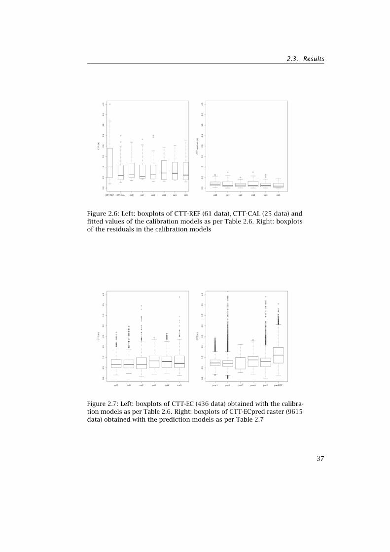
2.3. Results
Figure 2.6: Left: boxplots of CTT-REF (61 data), CTT-CAL (25 data) andfitted values of the calibration models as per Table 2.6. Right: boxplotsof the residuals in the calibration models
Figure 2.7: Left: boxplots of CTT-EC (436 data) obtained with the calibra-tion models as per Table 2.6. Right: boxplots of CTT-ECpred raster (9615data) obtained with the prediction models as per Table 2.7
37
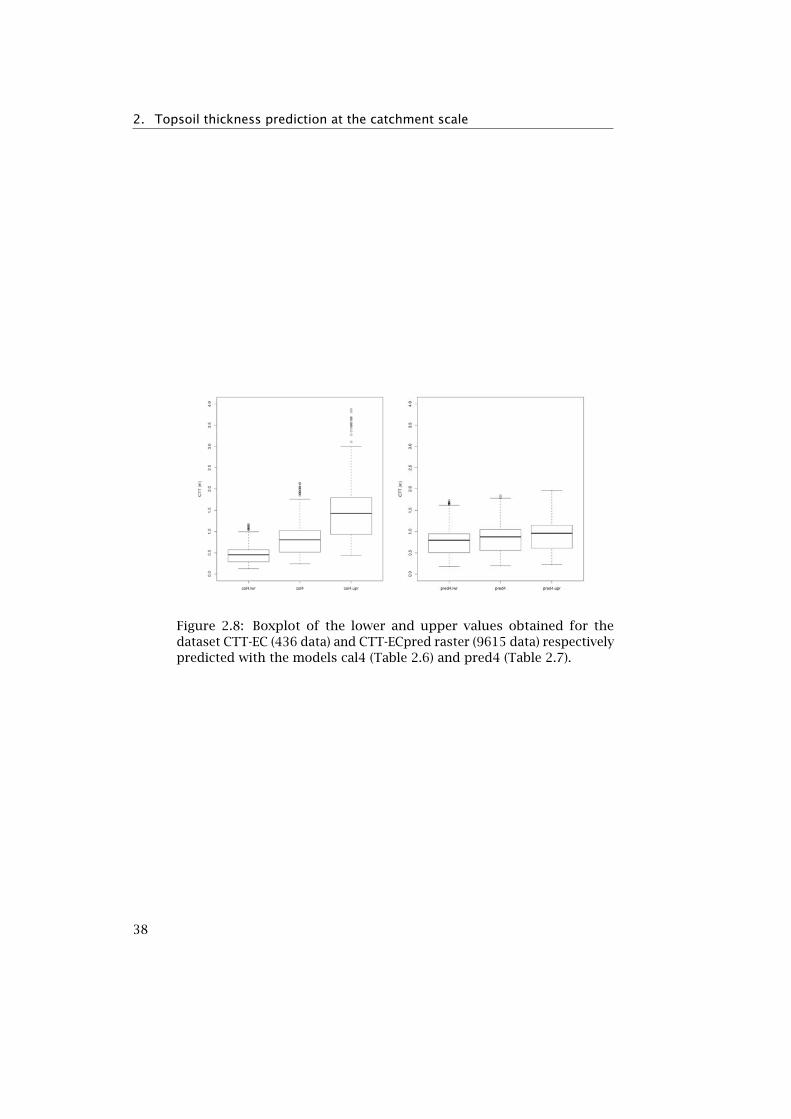
2. Topsoil thickness prediction at the catchment scale
Figure 2.8: Boxplot of the lower and upper values obtained for thedataset CTT-EC (436 data) and CTT-ECpred raster (9615 data) respectivelypredicted with the models cal4 (Table 2.6) and pred4 (Table 2.7).
38

2.3
.R
esults
Table 2.6: Calibration models based on CTT-CAL dataset and diagnostic results.
Model Predictor Sig.code(a)
Slope Inter. R2adj AIC BIC Residuals diagnostic
Selectedsub-geostat.MLM
(slope/inter.) Homo-scedasti-city(b)
Normality(c) No spatialcorrelation(d)
Chi-square
p-value+
W p-value+
Moran’sI
p-value+
cal0 ln(ECa) +++/+++ 0.96 -3.88 0.68 25.2 28.9 0.57 0.45 0.97 0.55 0.03 0.67 LR
cal1ln(ECa) +++/+++ 0.82
-3.36 0.72 23.0 27.8 0.53 0.47 0.98 0.81 -0.10 0.73 MLRTPI -/+++ -0.06
cal2
ln(ECa) +++/+++ 0.92
-3.77 0.86 5.74 11.8 0.42 0.52 0.97 0.54 -0.11 0.72 MLRMEANC +++/+++ -9.11
PLANC +++/+++ 0.22
cal3ln([ECa]CALCR) +++/+++
0.65-2.90
0.83 9.8 14.7 0.37 0.54 0.94 0.20 -0.14 0.58 ANOCOVAln([ECa]CLAY ) +++/+++ -2.31
cal4
ln([ECa]CALCR) +++/+++ 0.52-2.60
0.85 7.7 13.8 0.58 0.44 0.96 0.38 -0.29 0.17 ANOCOVA[TPI]CALCR -/+++ -0.04
ln([ECa]CLAY ) +++/+++ 0.52-2.00
[TPI]CLAY -/+++ -0.04
Continued on next page
39

2.
Topso
ilth
ickness
pred
iction
atth
ecatch
men
tscale
– continued from previous page
Model Predictor Sig.code(a)
Slope Inter. R2adj AIC BIC Residuals diagnostic
Selectedsub-geostat.MLM
(slope/inter.) Homo-scedasti-city(b)
Normality(c) No spatialcorrelation(d)
Chi-square
p-value+
W p-value+
Moran’sI
p-value+
cal5
ln([ECa]CALCR) +++/+++ 0.70
-3.18
0.92 -7.4 0.1 0.33 0.56 0.94 0.1 -0.21 0.35 ANOCOVA
[MEANC]CALCR ++/+++ -6.11
[PLANC]CALCR +++/+++ 0.17
ln([ECa]CLAY ) +++/+++ 0.70
-2.74[MEANC]CLAY ++/+++ -6.11
[PLANC]CLAY +++/+++ 0.17
+ p-value indicates the probability that the null hypothesis (in this case the model assumption) arose purely by chance. A value of 0.05indicates 95% of chance that the assumption is respected. (a) - Significance codes: 0 ’+++’ 0.001 ’++’ 0.01 ’+’ 0.05 ’-’ 0.1 ’x’ 1. (b) - ncv.testin car (Fox and Weisberg, 2011). (c) - Shapiro-Wilk test. (d) - Moran’s I (weight matrix computed following Lesch and Corwin, 2008).
40

2.3. Results
2.3.4 CTT prediction at the catchment scale
We predicted the CTT at the catchment scale on a grid of 25 m resolutionusing: (i) the CTT-EC datasets (Figure 2.7, left) computed in step 5 (Fig-ure 2.1) to obtain the CTT-ECpred rasters (step 6a, Figure 2.1); and (ii) theCTT-REF dataset to obtain the CTT-REFpred raster (step 6b, Figure 2.1).For each CTT-EC dataset obtained with the respective calibration model(Table 2.6), we computed the prediction models listed in Table 2.7 usingthe same auxiliary variables as in the calibration model (excluding theECa variable that was only available at the geophysical survey pointsand exclusively used for calibration). The model pred1 violated theassumption of homoscedasticity and was therefore not used in the pre-diction. In all the other models (pred2 to pred5), spatial-autocorrelationof the residuals was significant. We thus elaborated the variogram ofthe residuals and applied KED to predict CTT over the catchment. Allthe variograms of the residuals showed a relatively high nugget (∼50%of the total sill, which was between 0.05 and 0.15 [ln(m)]2), that can beexplained by the error associated with the ECa conversion into CTT. Theranges of the variograms of the models pred2 to pred5 were between403 and 850 m. CTT-REFpred raster was built with the model predREF(ANOCOVA) that incorporated the same predictors as the model pred4(Table 2.7). We next computed the ME, MAE and RMSE for all the CTT-ECpred rasters (i.e. pred2 to pred5) and for the CTT-REFpred raster usingthe same CTT-REF dataset. The summary statistics of the 5 CTT-ECpredand CTT-REFpred rasters, listed in Table 2.7, are shown in the boxplotsin Figure 2.7 (right). Models pred2 and pred5 showed long positive tailswith some CTT values > 4.0 m (not shown in the figure) and the highestRMSE (i.e. lowest accuracy). The model pred4 showed the lowest ME,MAE and RMSE, with values comparable to predREF. Note that ME ofpredREF (ANOCOVA model) is much lower (0.1 m) than the one of themodels pred2 to pred5 (KED models) since it corresponds to the mean ofthe residuals of the ANOCOVA model (that assumes normal distributionof the residuals with 0 mean). The prediction intervals computed atthe 95% confidence interval are presented in Figure 2.8 (right) for thepred4 model. Figures 2.9 and 2.10 show the CTT maps obtained withthe models predREF and pred4 respectively. The two patterns are nearlyidentical, due to the inclusion of the same auxiliary variables (TPI andRS-derived soil classes) in the prediction models. The CTT values of thepred4 model estimated using the geophysical data are lower than thevalues of the predREF model, because its calibration dataset (CTT-CAL)has lower CTT values than the CTT-REF dataset.
41

2.
Topso
ilth
ickness
pred
iction
atth
ecatch
men
tscale
Table 2.7: Prediction models based on CTT-EC (pred1 to pred5) and CTT-REF (predREF) datasets, and diagnostic results.
Model Cal.modelTable 2.6
Predictor Sig.code(a)
Slope Inter. R2adj AIC BIC Residuals diagnostic
(slope/inter.) Homo-scedasti-city(b)
Normality(c) No spatialcorrelation(d)
Chi-square
p-value+
W p-value+
Moran’sI
p-value+
pred1 cal1 TPI +++/+++ -0.34 -0.08 0.34 376.5 388.7 27.4 1E-7 0.99 0.04 0.59 0.00
pred2 cal2 MEANC +++/+++ -12.42-0.41 0.58 464.8 481.1 0.11 0.74 1.00 0.15 0.57 0.00
PLANC +++/+++ 0.22
pred3 cal3 CALCR N.A./+++ N.A. -0.830.67 87.5 99.8 0.81 0.37 1.00 0.19 0.59 0.00
CLAY N.A./+++ N.A. -0.02
pred4 cal4 [TPI]CALCR +++/+++ -0.05-0.76 0.76 -40.4 -24.1 6.54 0.01 1.00 0.66 0.60 0.00
[TPI]CLAY +++/+++ -0.02
pred5 cal5 [MEANC]CALCR +++/+++ -8.20-0.73
0.70 204.0 224.4 0.35 0.56 1.00 0.67 0.58 0.00[PLANC]CALCR +++/+++ 0.17
[MEANC]CLAY +++/+++ -8.20-0.14
[PLANC]CLAY +++/+++ 0.17
predREF∗N.A. [TPI]CALCR +++/+++ -0.11-0.49 0.56 105.9 114.9 1.01 0.32 0.98 0.17 0.12 0.15
[TPI]CLAY +++/+++ 0.27
Continued on next page
42

2.3
.R
esults
– continued from previous page
Model Cal.modelTable 2.6
Selectedsub-geostat.MLM
ME(m)
MAE(m)
RMSE(m)
pred1 cal1 LR mod. not valid:heteroscedast.
pred2 cal2 KED (det.model: MLR)
0.47 0.84 1.09
pred3 cal3 KED (det.model:ANOVA)
0.48 0.68 0.97
pred4 cal4 KED (det.model:ANOCOVA)
0.41 0.61 0.88
pred5 cal5 KED (det.model:ANOCOVA)
0.49 0.75 1.00
predREF∗N.A. ANOCOVA 0.10 0.58 0.76
N.A.: not applicable. + p-value indicates the probability that the null hypothesis (in this case the model assumption) arose purely bychance. A value of 0.05 indicates 95% of chance that the assumption is respected. ∗ the dependent variable in this model is CTT-REFdataset, while in the previous models it is CTT-EC. (a) - Significance codes: 0 ’+++’ 0.001 ’++’ 0.01 ’+’ 0.05 ’-’ 0.1 ’x’ 1. (b) - ncv.test in car(Fox and Weisberg, 2011). (c) - Shapiro-Wilk test. (d) - Moran’s I (weight matrix computed following Lesch and Corwin (2008)).
43

2.
Topso
ilth
ickness
pred
iction
atth
ecatch
men
tscale
Figure 2.9: CTT map obtained with predREF (CTT-REFpred raster) model (Table 2.7). CTT classes are shown using quartiles.
44

2.3
.R
esults
Figure 2.10: CTT map obtained with pred4 (CTT-ECpred raster) model (Table 2.7). CTT classes are shown using quartiles
45

2. Topsoil thickness prediction at the catchment scale
2.4 Discussion and conclusion
We presented a data-integration method to predict the CTT at the catch-ment scale based on: (i) invasive sampling; (ii) surface geophysics; (iii) RSimagery; and (iv) MLM. The invasive sampling was used as a referencedataset, the geophysics was applied to reduce the number of costly andtime-consuming invasive field measurements and the MLM was combinedwith the RS imagery and geophysical data to integrate the CTT variab-ility at the catchment scale. We predicted CTT at the catchment scaleusing 436 EM-31 ECa measurement points calibrated with 25 invasiveCTT measurements. The calibration and prediction processes were doneusing MLM and respective model diagnostics that allowed the integrationof the RS-derived soil classes and terrain attributes in the statistical mod-eling. We also predicted CTT using the 61 invasive CTT measurements ofthe CTT-REF dataset and the RS-derived auxiliary variables. We comparedthis prediction with the CTT prediction based on geophysical data.
We applied expedite, spatially- and cost-efficient RS methods basedon the interpretation of high resolution satellite and airborne imagery toderive soil classes and terrain parameters. Instead of using the availablebut unreliable soil map presented in Figure 2.2, we utilized a more repres-entative soil classification obtained from the interpretation of two fusedhigh resolution images (QB and AO) acquired in different seasons. Thesoil classification method was based on a multi-resolution segmentationof image objects and fuzzy logic (Benz et al., 2004). This supervised clas-sification corresponds to a semi-manual extraction of the image features,as it was necessary to digitize the training samples of 25% of the QBAOimage area to reach the target classification accuracy (95%). This methodhas the advantage of being repeatable and quantitatively assessed. How-ever, it does require technical knowledge and it can be time consuming.The terrain parameters were computed from the ASTER GDEM. Althoughthe geomorphological classification of the area into landforms can bedone by combining terrain parameters, it is subjective since the classesof the parameters to be related to landforms are arbitrary. To avoidthe introduction of artificial correlation, we preferred to directly usethe parameters in the statistical modeling. However, the morphometricterrain parameters MEANC, PLANC and PROFC, showed that outliers hada strong influence upon the statistical modeling. This is because thecomputing of the morphometric and the hydrological parameters integ-rate the elevation gradients between the actual cell and its 8 surroundingcells. They are thus very sensitive to artifacts in the ASTER GDEM, despitethe filtering of such errors is included in the terrain attribute algorithm.In contrast to the morphometric and hydrological parameters, the TPIcomputing is based on a large number of cells obtained by a user-definedbuffer range (in this study 500 m). TPI is thus less sensitive to the GDEMartifacts and better depicts the terrain geomorphology.
The geophysical data acquisition with the EM-31 device was quiteefficient and adequate for the high electrical conductivity of the CTT.
46

2.4. Discussion and conclusion
However, in more resistive conditions the geophysical survey would needto be adapted by substituting the FDEM method for another one, forinstance the ER, which however would imply a reduction of efficiency.In our study case, we performed 436 EM-31 survey locations along geo-physical transects transversal to the drainage features of the catchment(Figure 2.3) to capture the CTT spatial variability. In our first attemptto extract the CTT from the ECa data (Francés, 2008), we used 10 ECameasurements at each survey location to constrain the geophysical datainversion, which in turn allowed us to retrieve the depth-wise ECa soilprofiles. However, the extraction of the CTT based on the interpretationof the ECa inverted profiles, guided by the CTT field observations, provedto be highly subjective, not repeatable, and time-consuming. In addition,the uncertainties were not quantifiable. As that method was not suitablefor the objective of this study, instead we implemented a new approachbased on the statistical modeling of the relationship between CTT andECa. The 10 ECa measurements were highly inter-correlated and hadsimilar correlation with the CTT. To avoid collinearity effect in the statist-ical models, we selected only one representative ECa measurement madewith the EM-31 on the ground with horizontal coil, corresponding to thepenetration depth of ∼2.75 m. As the LR between CTT and ECa showeda good relationship (R2
adj of 0.68), the statistical modeling was suitableto convert the ECa data into CTT. In further studies we recommend theacquisition of two ECa measurements at each survey location insteadof 10. Two measurements permit to verify the consistency of the fieldmeasurements and to increase the number of survey locations, which ishighly valuable for studies at catchment scales that require large datacoverage.
For the calibration of the ECa data and the CTT prediction, we testedseveral statistical models derived from the MLM approach (Table 2.6and Table 2.7) using several combinations of the geophysical data andthe RS-derived auxiliary variables. We selected the most appropriatecalibration and prediction models by verifying the assumptions withdiagnostic tools and by assessing the goodness of fit. The validation ofthe statistical models, in particular the assumptions of homoscedasti-city and normality of the residuals, allowed us to take into account theerror propagation throughout the modeling process. The calibration ofthe ECa data with the 25 CTT and ECa pair-points (CTT-CAL) providedgood results, with R2
adj equal to 0.85 for the model cal4 (Table 2.6). Thebest CTT-ECpred prediction model (RMSE of 0.88 m) was obtained withKED and ANOCOVA model (pred4) that integrated the RS-derived soilclasses and TPI as auxiliary variables (Table 2.7). We also computed theCTT prediction model predREF, exclusively using the 61 invasive CTTmeasurements of the CTT-REF dataset (i.e. without geophysics data andcalibration process). This was done using ANOCOVA model that integ-rated the RS-derived soil classes and TPI as auxiliary variables (Table 2.7).For this reason, the two maps (Figures 2.9 and 2.10), i.e. CTT-ECpredderived from cal4 and CTT-REFpred derived from predREF, have a similarpattern that successfully depict the spatial variability of the CTT along
47
2. Topsoil thickness prediction at the catchment scale
the geomorphologic catchment features. They show similar RMSE (0.88 mfor pred4 and 0.76 m for predREF). However, CTT-ECpred derived frompred4 showed lower CTT values than CTT-REFpred. This is because thecalibration dataset (CTT-CAL) used to convert the geophysical data intoCTT also showed lower values than the reference observation dataset(CTT-REF) and because the ln transformation of the estimated variableshad an attenuation effect on higher values. The sampling scheme of ECaand invasive CTT measurements were based on purposive sampling. Thisoption was imposed because most of the invasive CTT measurementswere inherited from a previous study (39 data points). We complementedthis dataset by arbitrarily selecting 22 other points along the geophysicaltransects in order to cover the geomorphologic catchment features. Amore elaborated sampling scheme presented by Hengl et al. (2003b)based on the analysis of the feature and geographical spaces of auxiliaryvariables could be attempted in future studies. However, as the relation-ship between the target variable and the predictor is unknown a-priori,the sampling can be biased by an incorrect selection of uncorrelatedpredictors.
In this study, the objective was to derive efficiently a map that depictsthe CTT spatial variability at the catchment scale. The CTT was recog-nized as a major controlling factor in the hydrological processes and wasused as input for a hydrological distributed model (Chapter 5, Francésand Lubczynski, 2015) that computes groundwater recharge. This modelfollows a lumped-parametric approach, in which the reservoir paramet-ers lose their physical meaning and the model calibration correspondsto parameter fitting. As the CTT, in conjunction with the soil hydraulicparameters, are optimized during the calibration process, the eventualunderestimation of the CTT obtained with the best statistical predictionmodel (pred4) is not critically relevant for the performance of the hydro-logical model. This implies that CTT-ECpred using pred4 model can beconsidered as good as the CTT-REFpred and that the presented methodo-logy is suitable for hydrological and environmental studies. In hydrology,where catchments often need to be investigated over large areas, theproposed method could be particularly useful, because it minimizes thelabor-intensive field data acquisition and provides useful and acceptableresults.
48
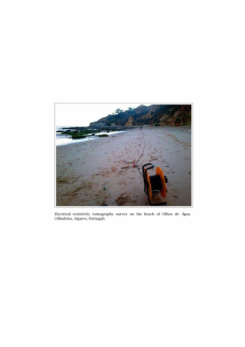
Electrical resistivity tomography survey on the beach of Olhos de Água(Albufeira, Algarve, Portugal).


3Contributions of hydrogeophysicsto the hydrogeological conceptualmodel of the Albufeira-Ribeira deQuarteira coastal aquifer inAlgarve, Portugal
3.1 Introduction
Coastal areas aggregate ∼50 % and ∼75 % of the world’s and Portugalpopulation respectively (Creel, 2003; Presidência do Conselho de Minis-tros, 2009). They concentrate economic activities related to harbors andmaritime transport, being also often propitious to the development ofbeach tourism. In these areas, water supply to domestic, agricultural,industrial and tourism sectors is generally provided by coastal aquifers(CA). The increase of permanent population and tourists during dry sea-son constitutes a tremendous pressure on the CA groundwater resources.Besides threats common to any aquifer, such as overexploitation, pollu-tion by waste water or leaching of contaminates, decrease of groundwaterrecharge due to climate change and soil impermeabilization in urbanareas, CA are also vulnerable to seawater intrusion and upconing thatcause freshwater salinization (Post, 2005; Dörfliger, 2013).
The protection of groundwater resources in coastal areas and theirsustainable management, in conjunctive use with other water resources(e.g. surface water, desalinized seawater), require the understandingof the CA hydrogeology. Since the late XIX century with the work ofBaden Ghijben (1888-1889), complemented by Herzberg (1901), hydro-geologists developed tools to study CA, such as analytical models (see
This chapter is based on: Contributions of hydrogeophysics to the hydrogeologicalconceptual model of the Albufeira-Ribeira de Quarteira coastal aquifer in Algarve, Por-tugal. Francés, A. P., E. Ramalho, J. Fernandes, M. Groen, R. Hugman, M. A. Khalil, J. DePlaen, and F. A. Monteiro Santos (2015), Hydrogeology Journal, accepted (April 2015)
51
3. Hydrogeological conceptual model of a coastal aquifer
examples in Fetter, 2001; Oude Essink, 2001; Dingman, 2002), numericalmodels of variable-density flow and solute transport (Bakker and Schaars,2005; Langevin et al., 2007), field data acquisition methods including air-borne and ground-based geophysics (Auken et al., 2010; Henderson et al.,2010; Kok et al., 2010; Faneca Sanchez et al., 2012) and automatic dataacquisition systems that allow high-resolution monitoring of groundwa-ter level, temperature and salinity (Poulsen et al., 2010; Dörfliger, 2013).These tools allowed to identify and map CA occurrences (Fleury et al.,2007; Custodio, 2010, and other papers of the "Saltwater and freshwa-ter interactions in coastal aquifers" issue of Hydrogeology Journal), aswell as to a better understanding of their dynamics (Aunay et al., 2007;de Montety et al., 2008; Oude Essink et al., 2010; Post and Abarca, 2010;Dörfliger, 2013; Werner et al., 2013) and to improve their management(Aunay et al., 2006; Barazzuoli et al., 2008). However, there are stillscientific challenges to be solved in order to support the resolution ofcritical situations. Following Post (2005), these challenges are grouped in:(i) conceptual issues; (ii) mathematical models; and (iii) subsurface char-acterization. Indeed, the theoretical conceptual model of the steady-statefreshwater-saltwater interface (FSWI) is more an exception than a rule.The position of the FSWI is ruled by highly dynamic processes, superim-posed on the regional and local geology, and varies spatio-temporally. Insome cases, it results in deep submarine groundwater discharge (SGD)and in other cases in continental brackish springs with elevation aboveseawater level. It was shown that the interface position and fresh andsaline groundwater distribution is also a result of sea transgression andregression at long time scale, i.e. hundreds of thousands of years (Post,2005; Fleury et al., 2007; Post et al., 2013). Multilayered aquifers sep-arated by aquitard and aquiclude, as well as geological settings suchas karstification, complicate the theoretical framework. Mathematicalmodels of variable-density groundwater flow may help in understandingthe aquifer dynamics and support management decisions. Such modelsrequire parametric and geometry knowledge of the aquifer obtained bysubsurface characterization methods. These subsurface data are gen-erally scarce because invasive methods such as borehole drilling andassociated aquifer tests are expensive and time-consuming. Moreover,the hydrogeological information is often missing from the existing com-mercial boreholes. Non-invasive hydrogeophysical methods of subsur-face data acquisition provide an alternative or a complement to directobservations, although the measured geophysical parameter has to behydrogeologically interpreted. As each hydrogeophysical method hasits own characteristics and capability, their complementary use covers awide range of hydrogeological problems, including those specific to CA.
In this study, hydrogeophysical methods were applied to contrib-ute to the development of the hydrogeological conceptual model of theAlbufeira-Ribeira de Quarteira (ARQ) CA (Algarve, southern Portugal). Inparticular, the specific objectives were: (i) to identify the water-bearinglayers and aquitards and relate them with the geological formations; and(ii) to detect the FSWI position along the coast line. The hydrogeophysical
52
3.2. Study area
results were interpreted using a regional piezometric map and boreholelithological logs as auxiliary information. Finally, the current data wereintegrated with offshore data from other studies to extend the hydrogeo-logical conceptual model to the offshore proximal shelf and explain thespatial distribution of the inter- and subtidal groundwater discharge.
3.2 Study area
The study area is located in the Algarve region, the southernmostprovince of Portugal (Figure 3.1), characterized by a warm Mediterranean,semi-arid climate. The Algarve mean annual temperature and precipita-tion are around 17°C and 600 mm, respectively. The precipitation regimeis irregular, having intermittent periods with heavy rains in the winterand a long dry period in the summer.
The southern coast of Portugal is characterized by an important de-velopment of the tourism sector, particularly demanding in water supplydue to the irrigation of numerous hotels, resorts and golf courses flank-ing the coast. Furthermore, water abstraction for agricultural purpose isalso significant. Vegetation is mainly composed by citrus trees used forcultivation and other commercially attractive trees such as olive, almondand cork oak trees.
The geomorphology of the Algarve littoral is characterized in theeast by a shoreline of sandy deposits and in the west by a limestone-dominated platform forming a cliff. Inland, the area can be described asa coastal plain with low relief, limited at north by Jurassic limestoneswith a more pronounced relief. Characteristic karstic features such asdolines and dry valleys can be observed.
3.2.1 Regional geology and hydrogeology
The onshore Meso-Cenozoic Algarve basin is an east-west trending sedi-mentary basin filled with ∼4000 m thick sediments lying on Carbonifer-ous schists and greywackes. Discordantly on the paleozoic substratum,sandstones and conglomerates of the "Arenitos de Silves" depositedduring the middle to upper Triassic, followed by the "Complexo PelíticoCarbonatado-Evaporítico". This sedimentary cycle ends with a volcanic-sedimentary complex related to the first rifting phase (Manuppella, 1992).These formations, together with the Carboniferous formations, constitutean impermeable substratum.
During the Lias, limestones and dolomites (600 m thick) depositedin central Algarve, extending from Lagoa to Tavira. The transition tothe Dogger is marked by an erosional phase followed by depositionof oolitic limestones and marls (350 to 500 m of thickness). Lias andDogger formations are the most important aquifers of the region, beingcharacterized by favorable hydraulic properties, large thickness and largeoutcrops (e.g. M5 aquifer in Figure 3.1). Moreover, these formations were
53
3. Hydrogeological conceptual model of a coastal aquifer
affected by an intense secondary dolomitization process that producedsecondary porosity and permeability (Almeida et al., 2000).
During the Malm, mainly in the upper Oxfordian-lower and middleKimmeridgian, the variation between sedimentary environments increaseddue to a second phase of rifting. From the upper Kimmeridgian on, aninner platform environment developed, promoting thick regressive car-bonate sequences with maximum expression in the Tithonian-Cretaceous.These formations have favorable hydrogeological properties and supportimportant aquifer systems, namely the Albufeira-Ribeira de Quarteira(ARQ) aquifer system (M6 in Figure 3.1, see also Table 3.1).
The transition to the Cretaceous is marked by a marine and fluvialsedimentation, while in the lower Aptian the subsidence increases andbegins a transgressive episode due to the North Atlantic expansion.The lower Cretaceous sediments are composed by marls, limestones,dolostones and a few sandy and conglomeratic levels (Rey, 2006, seeTable 3.1). Hydrogeologically, they are less favorable than the Jurassicformations, but can in some cases support aquifers when sufficientlythick and extensive.
The Lagos-Portimão Formation (Table 3.1) corresponds to deposits ofcarbonate platform, developed during a long time span (lower Burdigalianto upper Serravallian). It overlies the Carboniferous, Jurassic, Cretaceousand possible Paleogene units with angular unconformity, stratigraph-ical hiatuses or paraconformaties (Pais et al., 2000). Hydrogeologically,this highly karstified formation is very productive and constitutes animportant source for freshwater supply and irrigation (Almeida et al.,2000). Next to this formation, the sedimentation conditions passed fromcarbonate to siliciclastic environments during the lower Tortonian withthe deposition of the Olhos de Água Sands (Pais et al., 2000).
The Faro-Quarteira Sands (Table 3.1) corresponds to quaternary con-tinental sedimentation of siliciclastic deposits with reddish colors (50 mmaximum thickness). This formation covers most of the Algarve region,being largely exploited for irrigation purposes through traditional largewells called "noras".
54

3.2
.Stu
dy
area
Figure 3.1: Geological map of the study area adapted from Manuppella (1992). The dark grey structural map is from Terrinhaet al. (2014). The black, dashed rectangle indicates the location of Figure 3.3. Aquifer management units (Almeida et al., 2000):M4 - Ferragudo - Albufeira; M5 - Querenca - Silves; M6 - Albufeira - Ribeira de Quarteira; M7 - Quarteira. Geological faults: GF1 -Sagres-Algoz-Vila Real de Santo António flexure; GF2 - Quarteira fault; GF3 Albufeira fault; GF4 - Oura fault; GF5 - Mosqueirafault; GF6 - Olhos de Água fault. Coordinates system (also in next figures): UTM N29, WGS 84.
55

3.
Hyd
rogeo
logical
concep
tual
model
of
aco
astalaq
uifer
Figure 3.2: Geological cross-sections (location in Figure 3.1). Top: Manuppella (1992); bottom: (Manuppella et al., 2007).Abbreviations explained in Table 3.1.
56

3.2
.Stu
dy
area
Table 3.1: Lithostratigraphy and hydrostratigraphy of the study area adapted from Almeida and Lourenço da Silva (1990);Manuppella (1992); Almeida et al. (2000); Pais et al. (2000); Rey (2006).
Epoch Age Symb. Formation Lithology Thick. Mainlithology
Hydrostrati-graphy
Pleistocene? ? Qa Faro-Quarteira sands Clayey sandstones withpebbles intercalations
10-30 m Detrital Aquitard PQ
Pliocene Piazencian MOA Olhos de Água sands Feldspathic sands, pebbles
Miocene Burdigalian-Serravian
MLP Lagos-PortimãoForma-tion
Biocalcarenites, yellow orpink, sandy limestones andsandstones
30-85 m Limestone Aquifer MIO
LowerCretaceous
Aptian C2 Porto de Mós marls andlimestones; Luz marls;Limestones and marlswith Palorbitolina len-ticularis
Marls and limestones;Green and purple marls;Massive limestones andmarls, brownish
100 m Marl andlimestone
AquitardCRET
Barremian C2 Marls with Choffatelladecipiens
Marls, sandstones, marlylimestones and dolomites
50 m
Berriasian C1 Limestones with Choffa-tella pyrenaica; Sobralsandstones; Limestoneswith Trocholina; Pur-beck facies marls andlimestones
Limestones and marls,yellow to purple;Sandstones with quartzgravels, pebbles andpelites, reddish to purple;Oolithic limestones;Limestones, conglomerates,marls and dolomites
100 m Detrital
Continued on next page57
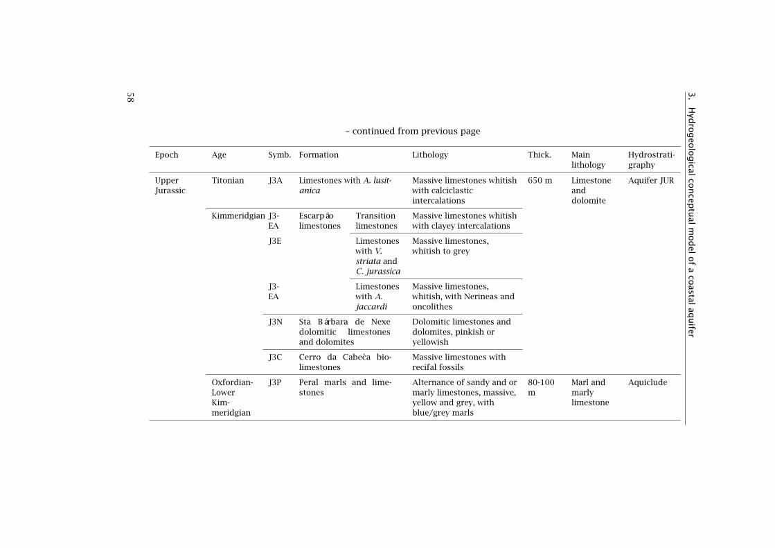
3.
Hyd
rogeo
logical
concep
tual
model
of
aco
astalaq
uifer
– continued from previous page
Epoch Age Symb. Formation Lithology Thick. Mainlithology
Hydrostrati-graphy
UpperJurassic
Titonian J3A Limestones with A. lusit-anica
Massive limestones whitishwith calciclasticintercalations
650 m Limestoneanddolomite
Aquifer JUR
Kimmeridgian J3-EA
Escarpãolimestones
Transitionlimestones
Massive limestones whitishwith clayey intercalations
J3E Limestoneswith V.striata andC. jurassica
Massive limestones,whitish to grey
J3-EA
Limestoneswith A.jaccardi
Massive limestones,whitish, with Nerineas andoncolithes
J3N Sta Bárbara de Nexedolomitic limestonesand dolomites
Dolomitic limestones anddolomites, pinkish oryellowish
J3C Cerro da Cabeca bio-limestones
Massive limestones withrecifal fossils
Oxfordian-LowerKim-meridgian
J3P Peral marls and lime-stones
Alternance of sandy and ormarly limestones, massive,yellow and grey, withblue/grey marls
80-100m
Marl andmarlylimestone
Aquiclude
58

3.2. Study area
3.2.2 Hydrogeology of the Albufeira-Ribeira de Quarteira (ARQ)aquifer system
The Albufeira-Ribeira de Quarteira (ARQ) aquifer system (M6 in Figure 3.1,54.6 km2) was characterized by Almeida and Lourenço da Silva (1990) andAlmeida et al. (2000). The latter defined the limit of the ARQ (Figure 3.1,shown as Manag. unit) and other regional aquifers, with the aim ofdefining inventory and management units for the national and local waterauthorities. The water-bearing formations are composed by detrital-carbonate rocks dating from Miocene and Upper Jurassic (Table 3.1and Figure 3.1). Both aquifers, henceforth MIO and JUR respectively,are generally separated by the Cretaceous aquitard (CRET), as shownin Figure 3.2 (bottom). However, in some sectors, depositional andstructural conditions allow the contact between the two water-bearingformations, making hydraulic connection possible (Almeida et al., 2000).Between Albufeira and the Quarteira stream, the sub-tabular Miocene tiltsslightly towards south-southeast (Figure 3.2 bottom). Miocene formationssedimented with a strong angular unconformity over the Cretaceous andJurassic formations (Figure 3.2 bottom). They are partly recovered by thePlio-quaternary formations that act as an aquitard, confining unit (PQaquitard).
The diapir west of Albufeira (Figures 3.1 and 3.2 top) caused a stronglocal angular unconformity (near 90°) between the Miocene and Creta-ceous formations. Another not outcropping salt diapir, but whose pres-ence is revealed by the groundwater hydrogeochemical characteristics, islocated east of Escarpão, extending southwards to the vicinity of Patã deBaixo, i.e. along the east border of the ARQ (Figure 3.1) and Quarteirastream (Almeida et al., 2000; Bronzini, 2011).
The aquifer system boundaries are defined by three tectonic majoraccidents (Figure 3.1):
• East: the northwest-southeast Quarteira fault (GF2), which condi-tioned the Miocene sedimentation as evidenced by a thicker easterncompartment (180 m, M7 aquifer) as compared to the western com-partment (80 m, ARQ-M6 aquifer). The boundary is located alongthe Quarteira stream that constitutes a discharge area, although itmay also be influent in its northern section (Almeida et al., 2000;Reis et al., 2007);
• North: west-east Sagres-Algoz-Vila Real de Santo António flexurezone (GF1, Figure 3.2 top);
• West: north-south Albufeira fault and Albufeira diapir (GF3 andDIAPIR, Figure 3.2 top).
The southern boundary is formed by the seacoast. The ARQ dischargesinto the sea through inter- and subtidal springs of fresh/brackish watermainly located at Olhos de Água. The subtidal springs create at thesurface of the sea rounded shapes that are well detectable from thetop of the cliffs, giving their name to the village (Olhos de Água means"Water Eyes"). The electrical conductivity (EC) and temperature (T) of
59

3. Hydrogeological conceptual model of a coastal aquifer
subtidal springs located at ∼120 m from the base of the coastal cliffsof Olhos de Água (Figure 3.1) were measured by scuba diving survey(Encarnação et al., 2013). On July 2013, the subtidal springs EC was∼9000 µS.cm−1, i.e. 1.1 Ω.m, and the temperature was 19.8°C, while thesea water had a EC and temperature of ∼56000 µS.cm−1 (0.2 Ω.m) and21.5°C respectively. For comparison, EC from the MIO aquifer rangesbetween ∼800 and 1200 µS.cm−1, i.e. 8.3 Ω.m and 12.5 Ω.m respectively,with a groundwater temperature ∼19°C. The intertidal springs are alsoobservable on the beach at low tide. Their temperature is similar to theMIO groundwater and their EC is generally lower (∼3000 µS.cm−1, i.e.3.3 Ω.m) than the subtidal springs.
Transmissivity, estimated in 30 boreholes exploiting the MIO layer,ranges between 84 and 3080 m2.d−1, with an average of 540 m2.d−1
and median of 235 m2.d−1 (Almeida and Lourenço da Silva, 1990). TheMIO aquifer is strongly affected by karstification, observable on the out-crops cliffs along the coastline. Consequently, it shows a heterogeneousdistribution of hydraulic conductivity and secondary porosity, whichis indirectly confirmed by low hydraulic gradients between 0.005 and0.0005, and by seasonal fluctuations of the water level varying betweenfew meters to several tenths of meters.
Recharge of the ARQ aquifer system was originally estimated as8.7×106 m3.y−1 (Almeida et al., 2000), based on an average yearly rainfallof 550 mm and considering recharge rates of 50% and 15% for the JURand MIO aquifers respectively. Based on water balance modeling usingsoil type and vegetation covers and considering an average yearly rainfallof 593 mm, Monteiro et al. (2007b) computed a deep percolation of11.0×106 m3.y−1 (36% of the rainfall), being the JUR recharge rate morethan twice the MIO recharge rate.
Groundwater abstraction for public supply were 3.3×10⁶ m3.y−1
during year 1993 (Almeida et al., 2000). During year 1999 and forboth aquifers ARQ and Quarteira (M7 in Figure 3.1), this value was8.43×106 m3.y−1, which corresponds to 30% of estimated average an-nual recharge of these two aquifers (Hugman et al., 2014b). After 1999,public water supply was mainly ensured by surface water, althoughgroundwater was also episodically pumped in summer season to com-pensate dam surface water shortage. Almeida et al. (2000) assessed as3.5×106 m3.y−1 (∼12% of the estimated average annual recharge) thewater extractions for irrigation in 1979. However the volume of ground-water extracted by private wells is unknown and was not considered inthese studies.
Recently, numerical flow models were applied to quantify the inter-and subtidal groundwater discharge and the impact of changes in ground-water use (Monteiro et al., 2007b; Hugman et al., 2014b). These authorsused the ARQ management unit boundary shown in Figure 3.1 that wasdefined by Almeida et al. (2000).
60
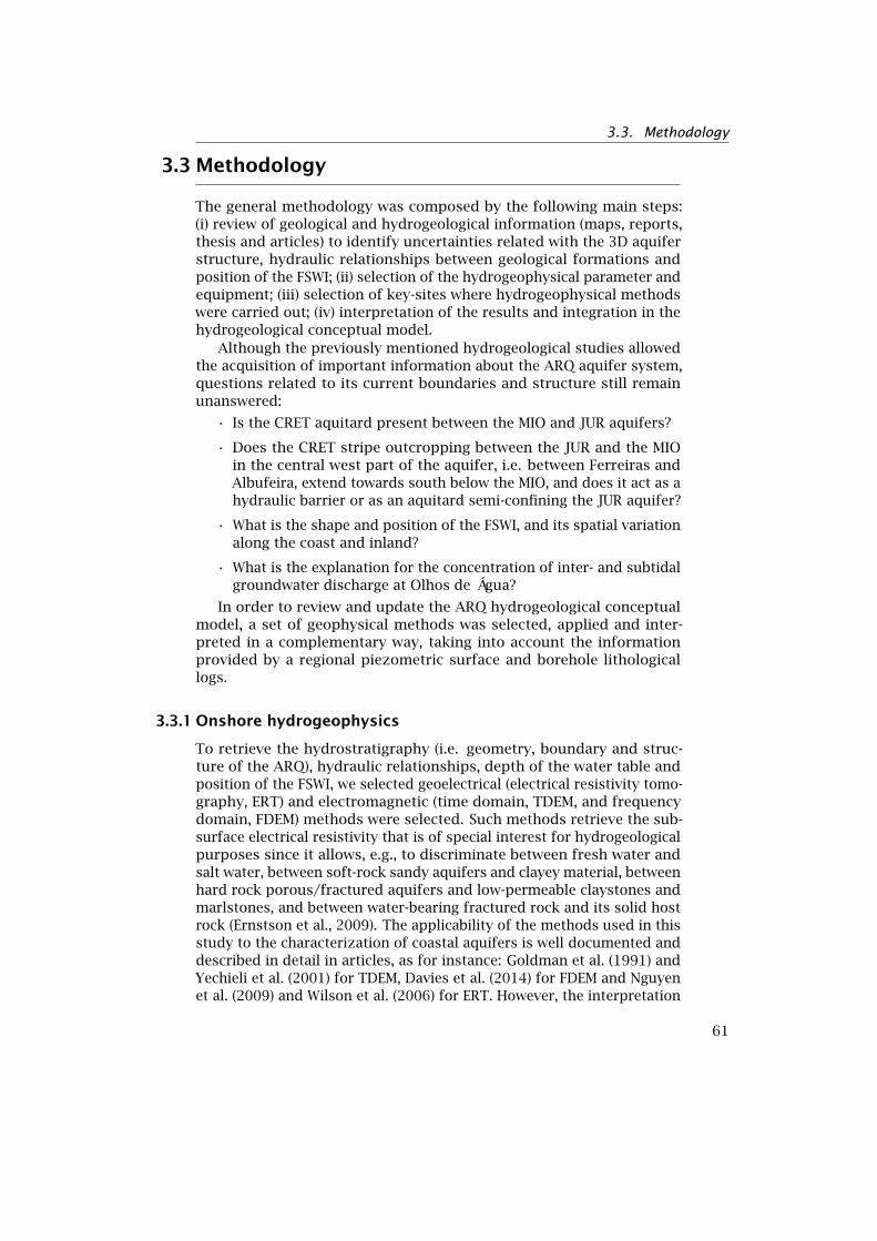
3.3. Methodology
3.3 Methodology
The general methodology was composed by the following main steps:(i) review of geological and hydrogeological information (maps, reports,thesis and articles) to identify uncertainties related with the 3D aquiferstructure, hydraulic relationships between geological formations andposition of the FSWI; (ii) selection of the hydrogeophysical parameter andequipment; (iii) selection of key-sites where hydrogeophysical methodswere carried out; (iv) interpretation of the results and integration in thehydrogeological conceptual model.
Although the previously mentioned hydrogeological studies allowedthe acquisition of important information about the ARQ aquifer system,questions related to its current boundaries and structure still remainunanswered:
• Is the CRET aquitard present between the MIO and JUR aquifers?
• Does the CRET stripe outcropping between the JUR and the MIOin the central west part of the aquifer, i.e. between Ferreiras andAlbufeira, extend towards south below the MIO, and does it act as ahydraulic barrier or as an aquitard semi-confining the JUR aquifer?
• What is the shape and position of the FSWI, and its spatial variationalong the coast and inland?
• What is the explanation for the concentration of inter- and subtidalgroundwater discharge at Olhos de Água?
In order to review and update the ARQ hydrogeological conceptualmodel, a set of geophysical methods was selected, applied and inter-preted in a complementary way, taking into account the informationprovided by a regional piezometric surface and borehole lithologicallogs.
3.3.1 Onshore hydrogeophysics
To retrieve the hydrostratigraphy (i.e. geometry, boundary and struc-ture of the ARQ), hydraulic relationships, depth of the water table andposition of the FSWI, we selected geoelectrical (electrical resistivity tomo-graphy, ERT) and electromagnetic (time domain, TDEM, and frequencydomain, FDEM) methods were selected. Such methods retrieve the sub-surface electrical resistivity that is of special interest for hydrogeologicalpurposes since it allows, e.g., to discriminate between fresh water andsalt water, between soft-rock sandy aquifers and clayey material, betweenhard rock porous/fractured aquifers and low-permeable claystones andmarlstones, and between water-bearing fractured rock and its solid hostrock (Ernstson et al., 2009). The applicability of the methods used in thisstudy to the characterization of coastal aquifers is well documented anddescribed in detail in articles, as for instance: Goldman et al. (1991) andYechieli et al. (2001) for TDEM, Davies et al. (2014) for FDEM and Nguyenet al. (2009) and Wilson et al. (2006) for ERT. However, the interpretation
61

3. Hydrogeological conceptual model of a coastal aquifer
of electrical resistivity survey is subject to the equivalence problem. Themeasured apparent resistivity is related with many physically equivalentmodels that may differ considerably. In other words, a given resistivitymay be the results of many combinations of resistivity and thickness ofoverlaid layers, and thus different resistivity models may fit the meas-ured data (Ernstson et al., 2009). Moreover, the measured resistivity valuedepends on the combination between the lithology and the water qualityof the geological medium. For instance, a clay layer saturated with freshwater may have the same electrical resistivity as a sandy layer saturatedwith salt water. It is thus important to interpret hydrogeophysical res-ults together with auxiliary information, such as borehole lithologicallogs. Another possibility to reduce the equivalence problem is to applymethods that measure another property of the medium. However, due tologistic and financial limitations, only geoelectrical and electromagneticmethods were applied.
The geoelectrical and electromagnetic hydrogeophysical surveys wereconducted between January and December 2013, comprising: (i) 17 TDEM(1D); (ii) 3 FDEM (2D); (iii) 11 ERT (2D). The surveys were organized in5 transects transversal and longitudinal to the main groundwater flowdirection (A, B, C, D and E in Figure 3.3). Note that the high urbandevelopment in the study area prevented the use of hydrogeophysicsin zones considered as important (e.g. lack of extension to deploy ERTcables or electromagnetic noise limiting the use of TDEM and FDEM).Specifically, the selected methods were used to detect: (i) position andslope of the FSWI using FDEM cross-sections perpendicular to the coast,TDEM on the coastal cliffs and ERT along the beach; (ii) water-bearingformations with TDEM and ERT; and (iii) the CRET aquitard below theMIO aquifer with TDEM and ERT. The ERT method was preferentially usedon the beach to detect shallow karstic structures and freshwater springsdue to its relatively high-resolution and cross-sectional characteristics.The delineation of the hydrostratigraphical units was based on electricalresistivity contrasts observed in the 2D FDEM and ERT cross-sections, aswell as on the 1D resistive layers obtained from the 1D TDEM inversion.
Table 3.2 resumes the main characteristics of the geophysical meth-ods that were used in this study, namely the devices, configurations andranges of investigation depths. Next the configurations that were appliedfrom each of the hydrogeophysical methods are presented.
3.3.1.1 Time domain electromagnetics method
A TEM-FAST 48 from Applied Electromagnetic Research (AEMR) companywas used with a square loop of 25 or 50 m side (1 turn) in coincidentloop configuration with an input current of 24 V and 4 A, allowing apenetration depth of 50 to 100 m, depending on the local geoelectricalprofile. A minimum of 3 curves at each site was acquired to confirm therepeatability of the measurement and the absence of EM noise inducedby galvanic and/or capacitive coupling (Danielsen et al., 2003). Thedata were inverted using the software TEM-RES v7 from AEMR. When
62

3.3. Methodology
necessary, noisy data were firstly removed. Afterwards, using automaticinversion and trial and error method, a theoretical curve was fitted onobserved data. The criterion of selection of the final solution was basedon the minimum number of layers for the same quality of fitting, as wellas hydrogeological knowledge of the area completed by local observationor borehole lithological logs and coherency with the other geophysicalmethods.
3.3.1.2 Frequency domain electromagnetics method
An EM-34 device from Geonics Instruments was used to perform 1Dsoundings every 20 m along profiles, allowing to retrieve 2D cross-sections. At each measurement point, the 1D vertical soundings werecarried out with 6 configurations, i.e. horizontal and vertical dipoleswith coil spacing of 10, 20 and 40 m (frequencies of 6.4, 1.6 and 0.4 kHz,respectively), which corresponds to theoretical investigation depths ran-ging between 7.5 and 60.0 m (Table 3.2). Based on these 1D soundingsalong profiles, the 2D geoelectrical modeling was conducted using thealgorithm EM34-2D, which applies a 1D laterally constrained method(Monteiro Santos, 2004). The inverse problem is solved using a smoothinversion, where each 1D conductivity model, obtained beneath eachmeasurement site, is constrained by its neighbors. The obtained 2Dcross-sections allow visualizing a model of the vertical distribution ofelectrical conductivities.
3.3.1.3 Geoelectrical method
ERT were acquired using an IRIS Syscal pro, an ABEM Terrameter SAS-4000 and a Scintrex TSQ-3 transmissor with a Elliot R-20A receiver. Thefirst one was configured with four 90 m long cables and a total of 72electrodes, the second with four 100 m long cables and a total of 64electrodes. Schlumberger and Wenner arrays were selected. Duringdata acquisition, the stacking option was activated to obtain at eachelectrode an electrical resistivity measurement with a standard deviationlower than 5%. The Scintrex TSQ-3 device was applied with 18 electrodesin dipole-dipole array with 1350 m length to detect large and deepgeological structures.
Inversions were carried out using RES2DINV v3.53 (Geotomo software,2010), using model refinement. Bad datum points and points with rootmean square error (RMSE) higher than 60 or 80% were removed from thefinal inversion.
The vertical accuracy of this method is relevant since the depthand thickness of the hydrostratigraphical units, as well as the depthof the groundwater table, was mostly derived from this method. Intheory, accuracy of the depth of the interface is obtained using sensitivitystudies (Geotomo software, 2010), which was not performed in this case.Applying to the distance inter-electrode the rule of thumb that definesthe depth of investigation as LERT /5, where LERT is the total ERT length
63

3. Hydrogeological conceptual model of a coastal aquifer
(Ernstson et al., 2009), one can obtain the resolution of the method.Therefore, the resolution for an inter-electrode distance of 5 m and 75 mis ∼1 m and ∼15 m respectively. Note that due to the specificity of themethod, this resolution degrades laterally and in depth.
64
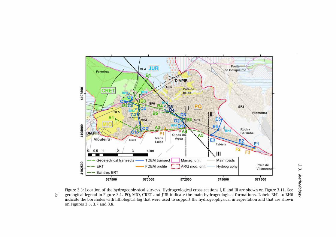
3.3
.M
ethod
ology
Figure 3.3: Location of the hydrogeophysical surveys. Hydrogeological cross-sections I, II and III are shown on Figure 3.11. Seegeological legend in Figure 3.1. PQ, MIO, CRET and JUR indicate the main hydrogeological formations. Labels BH1 to BH6indicate the boreholes with lithological log that were used to support the hydrogeophysical interpretation and that are shownon Figures 3.5, 3.7 and 3.8.
65

3.
Hyd
rogeo
logical
concep
tual
model
of
aco
astalaq
uifer
Table 3.2: Characteristics of the hydrogeophysical methods. All methods acquired the electrical resistivity (or its inverse, theelectrical conductivity).
Geophysical Method Device Configuration Investigationdepth Range
Dimension
Electrical ResistivityTomography (ERT)
IRIS - Syscal pro;ABEM -Terrameter
Schlumberger array;Wenner array
65-70 m 2D
Scintrex - TSQ-3 Dipole-dipole array 150 m 2D
Frequency DomainElectromagnetics(FDEM)
Geonics - EM-34 2D profiles based on 1Dsoundings every 20 musing horizontal andvertical dipoles at coildistance 10, 20 and 40 m
7.5 to 60.0 m 2D
Time DomainElectromagnetics(TDEM)
AEMR -TEM-FAST 48
25 to 50 m square loop 50-100 m 1D
66

3.3. Methodology
3.3.2 Auxiliary information
3.3.2.1 Hydraulic heads and regional static piezometric surface
The objective of the piezometric analysis was not to obtain a regionalpiezometric surface per se but to highlight high and low hydraulic gradi-ent areas and to detect hydraulic barriers, preferential groundwater flowzones and other relevant hydrogeological features.
The retrieval of a reliable static piezometric surface requires theavailability of a dense and uniform spatial distribution of boreholes andmeasurements made during a short period within the same hydrologicalconditions, which was not available in this study. Although a highborehole density was available in the ARQ costal aquifer, most of theboreholes were in activity and equipped with pumps, which did notallow us to use a dipper (high risk of blocking the dipper’s tape with thepump’s cables). Hydraulic heads measurements were only possible in22 boreholes of Albufeira Municipality (Câmara Municipal de Albufeira,CMA) that were equipped with dip tube. Hydraulic heads were alsoavailable from 69 boreholes belonging to the monitoring program of thePortuguese Environment Agency (Agência Portuguesa do Ambiente - APA,water resources information system available at http://snirh.pt). Thehistorical data from APA and CMA archives were thus compiled to obtainthe final hydraulic heads dataset of 91 boreholes composed with recordsfrom March 1978 to December 2013 (some of the boreholes are locatedoutside the area shown in Figure 3.1). The piezometric measurementsin the CMA boreholes were made after being deactivated, i.e. after 2001.They should correspond to the static piezometric level. However, dueto summer, episodic extractions, the quality of the measurements isuncertain, as some of them were carried out before the full recovery ofthe borehole.
The maximum number of concomitant hydraulic heads was only 29,with only 8 of them inside the ARQ area. As this dataset was insufficientto obtain a reliable interpolated surface, static piezometric surfaces wereelaborated using the minimum, median and maximum hydraulic headat each of the 91 boreholes. Simple kriging was applied to the datasetto retrieve the regional piezometric surface. In theory, the minimumhydraulic head is the most reliable value in absence of pumping, becausethe recession part of the well hydrograph follows an asymptotic expo-nential decay towards the local base level (Dingman, 2002). However inpractice, as some measurements were made few hours after long-termpumping, the minimum level may be biased, as it does not representthe static water level. To avoid misinterpretation and eliminate extremevalues, the regional piezometric map was elaborated using the medianhydraulic head at the 91 boreholes points. To avoid artifact in the southborder of the study area, the interpolation was constrained by definingthe groundwater table depth at sea level along the sea coast.
67
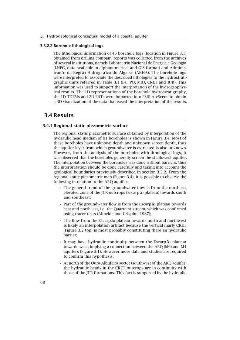
3. Hydrogeological conceptual model of a coastal aquifer
3.3.2.2 Borehole lithological logs
The lithological information of 45 borehole logs (location in Figure 3.1)obtained from drilling company reports was collected from the archivesof several institutions, namely Laboratório Nacional de Energia e Geologia(LNEG, data available in alphanumerical and GIS format) and Adminis-tração da Região Hidrográfica do Algarve (ARHA). The borehole logswere interpreted to associate the described lithologies to the hydrostrati-graphic units referred in Table 3.1 (i.e. PQ, MIO, CRET and JUR). Thisinformation was used to support the interpretation of the hydrogeophys-ical results. The 1D representations of the borehole hydrostratigraphy,the 1D TDEMs and 2D ERTs were imported into ESRI ArcScene to obtaina 3D visualization of the data that eased the interpretation of the results.
3.4 Results
3.4.1 Regional static piezometric surface
The regional static piezometric surface obtained by interpolation of thehydraulic head median of 91 boreholes is shown in Figure 3.4. Most ofthese boreholes have unknown depth and unknown screen depth, thusthe aquifer layer from which groundwater is extracted is also unknown.However, from the analysis of the boreholes with lithological logs, itwas observed that the boreholes generally screen the shallowest aquifer.The interpolation between the boreholes was done without barriers, thusthe interpretation should be done carefully and taking into account thegeological boundaries previously described in section 3.2.2. From theregional static piezometric map (Figure 3.4), it is possible to observe thefollowing in relation to the ARQ aquifer:
• The general trend of the groundwater flow is from the northern,elevated zone of the JUR outcrops (Escarpão plateau) towards southand southeast;
• Part of the groundwater flow is from the Escarpão plateau towardseast and northeast, i.e. the Quarteira stream, which was confirmedusing tracer tests (Almeida and Crispim, 1987);
• The flow from the Escarpão plateau towards north and northwestis likely an interpolation artifact because the vertical marly CRET(Figure 3.2 top) is most probably constituting there an hydraulicbarrier;
• It may have hydraulic continuity between the Escarpão plateautowards west, implying a connection between the ARQ (M6) and M4aquifers (Figure 3.1). However more data and studies are requiredto confirm this hypothesis;
• At north of the Oura-Albufeira sector (southwest of the ARQ aquifer),the hydraulic heads in the CRET outcrops are in continuity withthose of the JUR formations. This fact is supported by the hydraulic
68

3.4. Results
heads of 3 boreholes identified by BHa, BHb and BHc labels. Two ofthese boreholes are most probably implemented in the JUR aquifer:BHa was drilled inside a nora with 14.5 m depth, close to the con-tact CRET-JUR, where the CRET is very thin; BHc is ∼100 m deep,implemented in outcropping JUR formations. In agreement with thegeological cross-section of Figure 3.2 (top), these data indicates thatthe JUR aquifer extends in continuity from the northern outcrop-ping area towards the sea, below the CRET and the MIO formations,and that the GF3 is not a hydraulic barrier. For groundwater mod-eling purpose, the west border of the aquifer limit should thus beextended toward west, as shown in Figures 3.1, 3.3 and 3.4 (ARQmodeling unit);
• Groundwater flow is convergent towards a sink located betweenMaria Luisa and Olhos de Água, indicating preferential dischargearea and/or groundwater abstraction;
• The hydraulic gradient is higher in the JUR zone of the ARQ aquiferthan in the MIO aquifer, indicating higher hydraulic conductivity inMIO than in JUR.
69

3.
Hyd
rogeo
logical
concep
tual
model
of
aco
astalaq
uifer
Figure 3.4: Regional static piezometric map retrieved using the median hydraulic head of 91 boreholes (black label next to theborehole symbol indicates the number of values). GWT stands for groundwater table depth. The GWT elevation color bar isshow using 10 quantiles, meaning that each class corresponds to 10% of the values. The equidistance between equipotentiallines is 5 m.
70
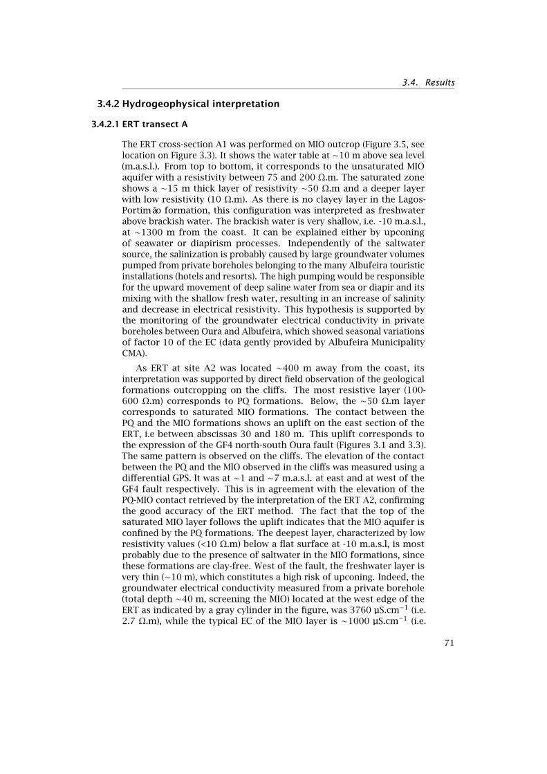
3.4. Results
3.4.2 Hydrogeophysical interpretation
3.4.2.1 ERT transect A
The ERT cross-section A1 was performed on MIO outcrop (Figure 3.5, seelocation on Figure 3.3). It shows the water table at ∼10 m above sea level(m.a.s.l.). From top to bottom, it corresponds to the unsaturated MIOaquifer with a resistivity between 75 and 200 Ω.m. The saturated zoneshows a ∼15 m thick layer of resistivity ∼50 Ω.m and a deeper layerwith low resistivity (10 Ω.m). As there is no clayey layer in the Lagos-Portimão formation, this configuration was interpreted as freshwaterabove brackish water. The brackish water is very shallow, i.e. -10 m.a.s.l.,at ∼1300 m from the coast. It can be explained either by upconingof seawater or diapirism processes. Independently of the saltwatersource, the salinization is probably caused by large groundwater volumespumped from private boreholes belonging to the many Albufeira touristicinstallations (hotels and resorts). The high pumping would be responsiblefor the upward movement of deep saline water from sea or diapir and itsmixing with the shallow fresh water, resulting in an increase of salinityand decrease in electrical resistivity. This hypothesis is supported bythe monitoring of the groundwater electrical conductivity in privateboreholes between Oura and Albufeira, which showed seasonal variationsof factor 10 of the EC (data gently provided by Albufeira MunicipalityCMA).
As ERT at site A2 was located ∼400 m away from the coast, itsinterpretation was supported by direct field observation of the geologicalformations outcropping on the cliffs. The most resistive layer (100-600 Ω.m) corresponds to PQ formations. Below, the ∼50 Ω.m layercorresponds to saturated MIO formations. The contact between thePQ and the MIO formations shows an uplift on the east section of theERT, i.e between abscissas 30 and 180 m. This uplift corresponds tothe expression of the GF4 north-south Oura fault (Figures 3.1 and 3.3).The same pattern is observed on the cliffs. The elevation of the contactbetween the PQ and the MIO observed in the cliffs was measured using adifferential GPS. It was at ∼1 and ∼7 m.a.s.l. at east and at west of theGF4 fault respectively. This is in agreement with the elevation of thePQ-MIO contact retrieved by the interpretation of the ERT A2, confirmingthe good accuracy of the ERT method. The fact that the top of thesaturated MIO layer follows the uplift indicates that the MIO aquifer isconfined by the PQ formations. The deepest layer, characterized by lowresistivity values (<10 Ω.m) below a flat surface at -10 m.a.s.l, is mostprobably due to the presence of saltwater in the MIO formations, sincethese formations are clay-free. West of the fault, the freshwater layer isvery thin (∼10 m), which constitutes a high risk of upconing. Indeed, thegroundwater electrical conductivity measured from a private borehole(total depth ∼40 m, screening the MIO) located at the west edge of theERT as indicated by a gray cylinder in the figure, was 3760 µS.cm−1 (i.e.2.7 Ω.m), while the typical EC of the MIO layer is ∼1000 µS.cm−1 (i.e.
71
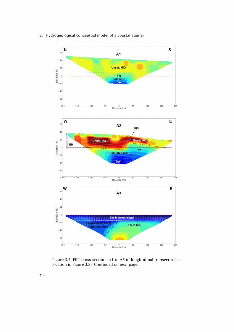
3. Hydrogeological conceptual model of a coastal aquifer
Figure 3.5: ERT cross-sections A1 to A5 of longitudinal transect A (seelocation in Figure 3.3). Continued on next page.
72

3.4. Results
– continued from previous page. BH stands for borehole (no log available),FW for freshwater, BW for brackish water, SW for saltwater, Unsat forunsaturated and Sat. for saturated. Other abbreviations are explained inthe text. Inversions of cross-sections A3 to A5 were performed withouttopography (flat beach). The elevation and distance scales are the samefor all cross-sections. The red horizontal line indicates the mean sealevel. Inversion root mean square errors (%): A1 1.0, A2 2.6, A3 1.5, A41.8, A5 1.5.
73

3. Hydrogeological conceptual model of a coastal aquifer
10.0 Ω.m).ERTs A3 to A5, conducted on the beach, present similar settings
between them: a low resistivity layer (<10 Ω.m) above a layer with resistiv-ity ranging from ∼20-100 Ω.m. The first layer corresponds to seawaterin beach sands while the second to fresh groundwater in MIO forma-tions. This configuration is explained by coastal fringe processes, suchas tidal dynamics and upper seawater recirculation zone (Werner et al.,2013). Karstic structures, expressed by blocks of different resistivity, arealso visible on ERT A3 and A4. An intertidal freshwater spring, clearlyidentified in the field, is visible on ERT A4 between abscissa -60 and 0.Finally, the deepening of the top of the MIO/base of the PQ towards eastis clearly visible from A4 to A5. However, PQ was expected between thesand beach and MIO, but either it is not present or its resistive signatureis similar to the sand beach saturated with saltwater, probably due tothe presence of saturated clayey lithology in PQ.
3.4.2.2 FDEM cross-sections
The FDEM cross-sections of Figure 3.6, all of them starting on the beach,show at south formations saturated with seawater, characterized by lowresistivity (<20 Ω.m) and, at north, freshwater saturated formations withresistivity of ∼20-50 Ω.m. At F1, the freshwater formations correspondto the MIO aquifer, while at F2 and F3 they correspond to alluvium, duneand beach sands. The slope of the FSWI is clearly imaged, showing asteep inclination at F1, while at F2 and F3, located in the eastern part ofthe AQR, the inclination is smooth. This geometry was expected sincethe hydraulic gradients are the lowest in the east sector (Figure 3.4).The relation between the hydraulic gradient and inclination of the FSWIcan be confirmed using analytical models (Baden Ghijben, 1888-1889;Herzberg, 1901; Glover, 1959). Below the Quarteira stream, at North-Eastof the F3 cross-section, the ∼20-50 Ω.m resistivity layer seems to indicatefresh groundwater. Above, the low resistivity layer indicates saltwaterintrusion from the Quarteira stream inside the alluvionar formations.This cross-section exemplifies the complex relationships between theMIO aquifer, the surficial alluvionar formations and the Quarteira streamthat is at this location strongly influenced by sea and tides.
74

3.4. Results
Figure 3.6: FDEM cross-sections (see location in Figure 3.3). FW standsfor freshwater, BW for brackish water and SW for saltwater. Otherabbreviations are explained in the text. The black dash line representsapproximately the location of the freshwater-saltwater interface (FSWI).These cross-sections show steep (F1) and smooth (F2 and F3) inclinedFSWI. All cross-sections started on the beach, located at south. The redhorizontal line indicates the mean sea level.
75
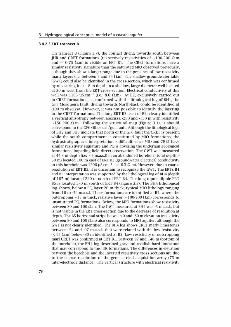
3. Hydrogeological conceptual model of a coastal aquifer
3.4.2.3 ERT transect B
On transect B (Figure 3.7), the contact diving towards south betweenJUR and CRET formations (respectively resistivities of ∼100-200 Ω.mand ∼10-75 Ω.m) is visible on ERT B1. The CRET formations have asimilar resistivity signature than the saturated MIO observed previously,although they show a larger range due to the presence of low resistivitymarly layers (i.e. between 5 and 75 Ω.m). The shallow groundwater table(GWT) could also be identified in the cross-section, which was confirmedby measuring it at ∼8 m depth in a shallow, large diameter well locatedat 30 m west from the ERT cross-section. Electrical conductivity at thiswell was 1165 µS.cm−1 (i.e. 8.6 Ω.m). At B2, exclusively carried outin CRET formations, as confirmed with the lithological log of BH1, theGF5 Mosqueira fault, diving towards North-East, could be identified at-100 m abscissa. However, it was not possible to identify the layeringin the CRET formations. The long ERT B3, east of B2, clearly identifieda vertical anisotropy between abscissa -250 and -150 m with resistivity∼150-200 Ω.m. Following the structural map (Figure 3.1), it shouldcorrespond to the GF6 Olhos de Água fault. Although the lithological logsof BH2 and BH3 indicate that north of the GF6 fault the CRET is present,while the south compartment is constituted by MIO formations, thehydrostratigraphical interpretation is difficult, since MIO and CRET havesimilar resistivity signature and PQ is covering the underlain geologicalformations, impeding field direct observation. The GWT was measuredat 44.8 m depth (i.e. ∼5 m.a.s.l) in an abandoned borehole (total depth >50 m) located 100 m east of ERT B3 (groundwater electrical conductivityin this borehole was 1206 µS.cm−1, i.e. 8.3 Ω.m). However, due to coarseresolution of ERT B3, it is uncertain to recognize the GWT. The ERTs B4and B5 interpretation was supported by the lithological log of BH4 (depthof 187 m) located 220 m north of ERT B4. The long dipole-dipole ERTB5 is located 170 m south of ERT B4 (Figure 3.3). The BH4 lithologicallog shows, below a PQ layer 26 m thick, typical MIO lithology rangingfrom 16 to -54 m.a.s.l. These formations are identified at B4, where theoutcropping ∼15 m thick, resistive layer (∼100-200 Ω.m) corresponds tounsaturated PQ formations. Below, the MIO formations show resistivitybetween 30 and 100 Ω.m. The GWT measured at BH4 was -5 m.a.s.l., butis not visible in the ERT cross-section due to the decrease of resolution atdepth. The B5 horizontal stripe between 0 and -80 m elevation (resistivitybetween 30 and 100 Ω.m) also corresponds to MIO aquifer, although theGWT is not clearly identified. The BH4 log shows CRET marly limestonesbetween -54 and -97 m.a.s.l. that were related with the low resistivity(< 15 Ω.m) below -80 m identified at B5. Low resistivity of outcroppingmarl CRET was confirmed at ERT B1. Between 97 and 146 m (bottom ofthe borehole), the BH4 log described gray and reddish hard limestonethat may correspond to the JUR formations. The differences in elevationbetween the borehole and the inverted resistivity cross-sections are dueto the coarse resolution of the geoelectrical acquisition array (75 minter-electrode distance). The vertical structure with electrical resistivity
76

3.4. Results
ranging from 100-200 Ω.m visible in the middle of B5 likely correspondsto the GF6 Olhos de Água fault. This GF6 fault is also identified in ERTB6 at abscissa 10 m. The same ERT B6, located ∼600 m north from thecoast, shows ∼20 m of PQ (resistivity of 150-700 Ω.m) on top of MIOformations (resistivity of 50-100 Ω.m), as confirmed by BH5. As in A2,the MIO aquifer is probably confined, although the water level indicatedin the drilling report was just below the interface MIO/PQ.
77

3. Hydrogeological conceptual model of a coastal aquifer
Figure 3.7: ERT cross-sections B1 to B6 of transversal transect B (seelocation in Figure 3.3). BH stands for borehole, Unsat. for unsaturated,FW for fresh water, GWT for groundwater table depth. Other abbrevi-ations are explained in the text. The elevation and distance scales arethe same for all cross-sections, as well as in Figure 3.5, expect for B3 andB5 (indicated with red labels). Continued on next page.78
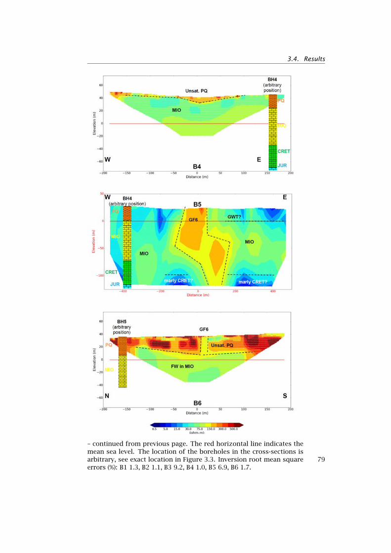
3.4. Results
– continued from previous page. The red horizontal line indicates themean sea level. The location of the boreholes in the cross-sections isarbitrary, see exact location in Figure 3.3. Inversion root mean squareerrors (%): B1 1.3, B2 1.1, B3 9.2, B4 1.0, B5 6.9, B6 1.7.
79
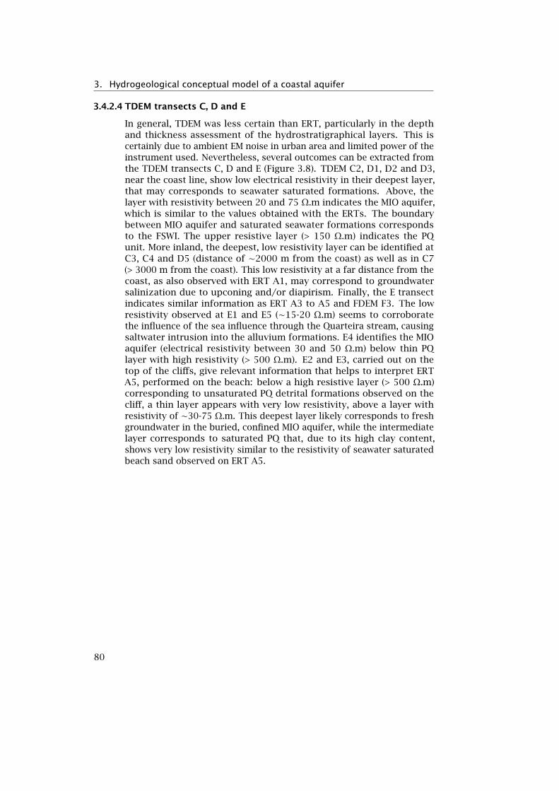
3. Hydrogeological conceptual model of a coastal aquifer
3.4.2.4 TDEM transects C, D and E
In general, TDEM was less certain than ERT, particularly in the depthand thickness assessment of the hydrostratigraphical layers. This iscertainly due to ambient EM noise in urban area and limited power of theinstrument used. Nevertheless, several outcomes can be extracted fromthe TDEM transects C, D and E (Figure 3.8). TDEM C2, D1, D2 and D3,near the coast line, show low electrical resistivity in their deepest layer,that may corresponds to seawater saturated formations. Above, thelayer with resistivity between 20 and 75 Ω.m indicates the MIO aquifer,which is similar to the values obtained with the ERTs. The boundarybetween MIO aquifer and saturated seawater formations correspondsto the FSWI. The upper resistive layer (> 150 Ω.m) indicates the PQunit. More inland, the deepest, low resistivity layer can be identified atC3, C4 and D5 (distance of ∼2000 m from the coast) as well as in C7(> 3000 m from the coast). This low resistivity at a far distance from thecoast, as also observed with ERT A1, may correspond to groundwatersalinization due to upconing and/or diapirism. Finally, the E transectindicates similar information as ERT A3 to A5 and FDEM F3. The lowresistivity observed at E1 and E5 (∼15-20 Ω.m) seems to corroboratethe influence of the sea influence through the Quarteira stream, causingsaltwater intrusion into the alluvium formations. E4 identifies the MIOaquifer (electrical resistivity between 30 and 50 Ω.m) below thin PQlayer with high resistivity (> 500 Ω.m). E2 and E3, carried out on thetop of the cliffs, give relevant information that helps to interpret ERTA5, performed on the beach: below a high resistive layer (> 500 Ω.m)corresponding to unsaturated PQ detrital formations observed on thecliff, a thin layer appears with very low resistivity, above a layer withresistivity of ∼30-75 Ω.m. This deepest layer likely corresponds to freshgroundwater in the buried, confined MIO aquifer, while the intermediatelayer corresponds to saturated PQ that, due to its high clay content,shows very low resistivity similar to the resistivity of seawater saturatedbeach sand observed on ERT A5.
80
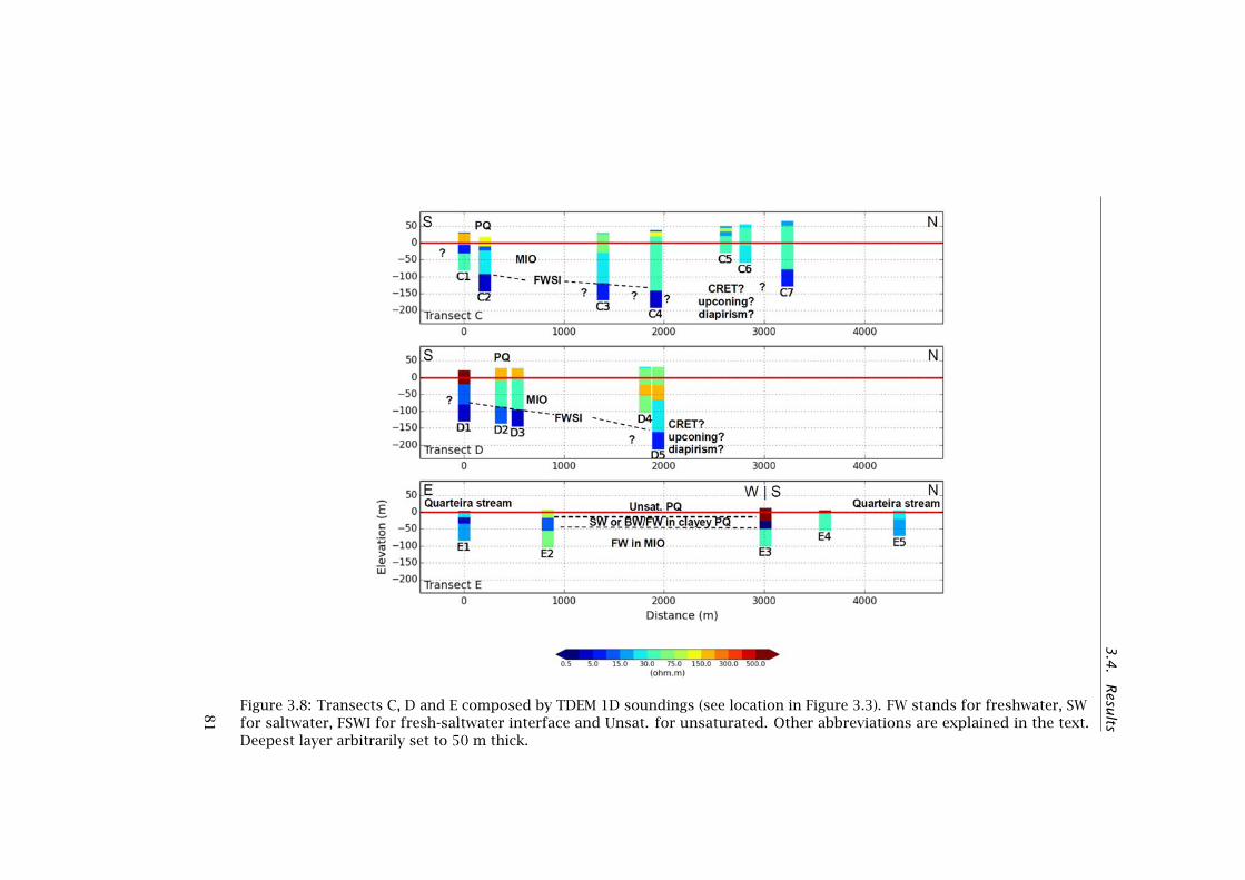
3.4
.R
esults
Figure 3.8: Transects C, D and E composed by TDEM 1D soundings (see location in Figure 3.3). FW stands for freshwater, SWfor saltwater, FSWI for fresh-saltwater interface and Unsat. for unsaturated. Other abbreviations are explained in the text.Deepest layer arbitrarily set to 50 m thick.
81
3. Hydrogeological conceptual model of a coastal aquifer
3.5 Discussion
3.5.1 Geoelectrical model
The resistivity range of the hydrogeological formations of the study areais presented in Table 3.3. A good agreement was observed among the3 geophysical techniques. TDEM and FDEM are more expedite than ERTto carry out in the field, although more sensitive to EM noise. However,ERT gives a detailed overview of the spatial relationship among the hy-drogeological formations at good resolution for the 5 m inter-electrodespacing. As referred earlier, TDEM is less certain than ERT in the depthand thickness assessment of the hydrostratigraphical layers. Moreover,layers detected at depth higher than ∼100 m should be carefully inter-preted taking into account the high uncertainty of the measured signal atthis depth, particularly in presence of ambient EM noise of urban areas.
The results presented in this study are in agreement with previousgeoelectrical surveys. Elsendoorn et al. (1982) presented a north-southgeoelectrical cross-section comprising 5 vertical electrical soundings(VES), located north of Olhos de Água and with ∼4 km long. In thiscross-section, PQ had resistivity ∼270 Ω.m, saturated MIO ∼110 Ω.m,upper CRET (C2 in Table 3.1) ∼25 Ω.m, and CRET C1 60-100 Ω.m. Theircross-section presents a sub-tabular PQ above MIO and CRET formations,diving towards south. The marly CRET was also identified by otherauthors in the Quarteira region, below the MIO (Geirnaert et al., 1982;Carvalho et al., 2006, 2012).
At some sites, the hydrogeophysical interpretation is still ambiguousdue to three main reasons: (i) insufficient depth of investigation limitedby the geophysical instruments and configurations used in this study;(ii) overlap of electrical resistivity signatures of geological formations,mainly MIO and CRET; and (iii) Archie’s law (Archie, 1942; Winsaueret al., 1952) is only valid for clean sand formations, which means thatkarstification and clay presence preclude its direct application. The use ofmore powerful TDEM than the one used in this study and complementarymethods, such as reflection seismics (Carvalho et al., 2012) or magneticresonance soundings (MRS) (Legchenko et al., 2009; Vouillamoz et al.,2012a), which target other rock properties (seismic wave propagationand presence of hydrogen ion, respectively), may be extremely useful toovercome the enunciated limitations.
3.5.2 Contributions to the hydrogeological conceptual model of theARQ aquifer system
The presence of the CRET between the MIO and the JUR formations seemsto be confirmed by the hydrogeophysics’ results of this study and thestudies previously cited. It is probable that the JUR aquifer recharges theMIO aquifer from below, due to higher hydraulic heads in the JUR thanin the MIO. This upward recharge may occur through the CRET aquitard,through fault zones or through direct contacts between JUR and MIO,
82

3.5. Discussion
Table 3.3: Geoelectrical range of the hydrostratigraphical units. PQ:Plio-quaternary; MIO: Miocene; CRET: Cretaceous; JUR: Jurassic; FW:freshwater; SW: saltwater; BW: brackish water.
Layer Resistivity range(ohm.m)
Location Resistivity(a)
(ohm.m)
Sand beach (SW) <10 A3-5
PQ unsat. 100-700 A1-2, B4, B6,C1-2, D1-5,E2-4
270
PQ sat. 10-15 A3-5, E2-3
MIO unsat. 75-200 A1
MIO sat. (FW) 20-100 A1-5, B4-6,C2-4, D1-3,E2-4, F1
110
MIO sat. (BW) 10-50 A1-5
MIO sat. (SW) <10-20 A2-3, C2-4,C7(?), D1-3,D5(?)
CRET 10-100 B1-2, B3(?),B5, C5-7
25 (C2) and60-100 (C1)
JUR unsat. 100-200 B1
(a) from Elsendoorn et al. (1982)
although this last configuration was not identified using hydrogeophysics.As there is an apparent geological and hydraulic continuity of the JURlayer below the CRET outcrop, it is proposed that, for groundwater flowmodeling, the west boundary of the ARQ management unit should beextended towards the Albufeira north-south fault (GF3), excluding theAlbufeira diapir (Figure 3.1, ARQ mod. unit).
Structural accidents affecting the MIO and CRET formations weredetected with the ERTs. The GF4, GF5 and GF6 faults do not constitutea hydraulic barrier, since the piezometric surface (Figure 3.4) is not af-fected. Some faults may have a strong influence in the hydrochemistryof the groundwater by acting as preferential flow channel of diapir ascen-sion or seawater intrusion. Groundwater salinization may be caused bysimultaneous sources of diapirism and seawater intrusion, as it has beenobserved in other coastal aquifers in the Mediterranean basin (Trabelsiet al., 2012; Mongelli et al., 2013). As seawater intrusion can be observedvery far from the coast inland, sometimes at 8 km (de Montety et al.,2008), it is challenging to distinguish diapiric and sea origins. Hydrogeo-chemical and isotopic surveys are generally required to recognize thesources of the salinization, including rock-water interactions, sea intru-
83

3. Hydrogeological conceptual model of a coastal aquifer
sion and anthropic activities (Vengosh et al., 1999; Alcalá and Custodio,2008; Bronzini, 2011; Mongelli et al., 2013).
The FSWI interface shape was expeditiously detected using the FDEMmethod, showing that on the west sector it is steepest than in the eastsector because of lower hydraulic gradient in this area.
Offshore data were also compiled from other studies to complementthe onshore observations. The map of the sea bottom of the Algarveinternal shelf (Braz Teixeira and Macedo, 2001, Figure 3.9) shows anoutcropping rocky sea bottom extending from Albufeira to Olhos deÁgua, with its south border in the southwest direction. Correlationwith the outcrops of the beach cliffs indicates that this rocky bottom iscomposed by MIO formations. At east, these MIO formations are coveredby offshore sands that overlay the PQ formations. This description iscorroborated by a seismic profile (Fig. 3.10) that evidenced the offshoreMIO outcropping at the proximal shelf, while at east the offshore MIOformations are confined by PQ.
84
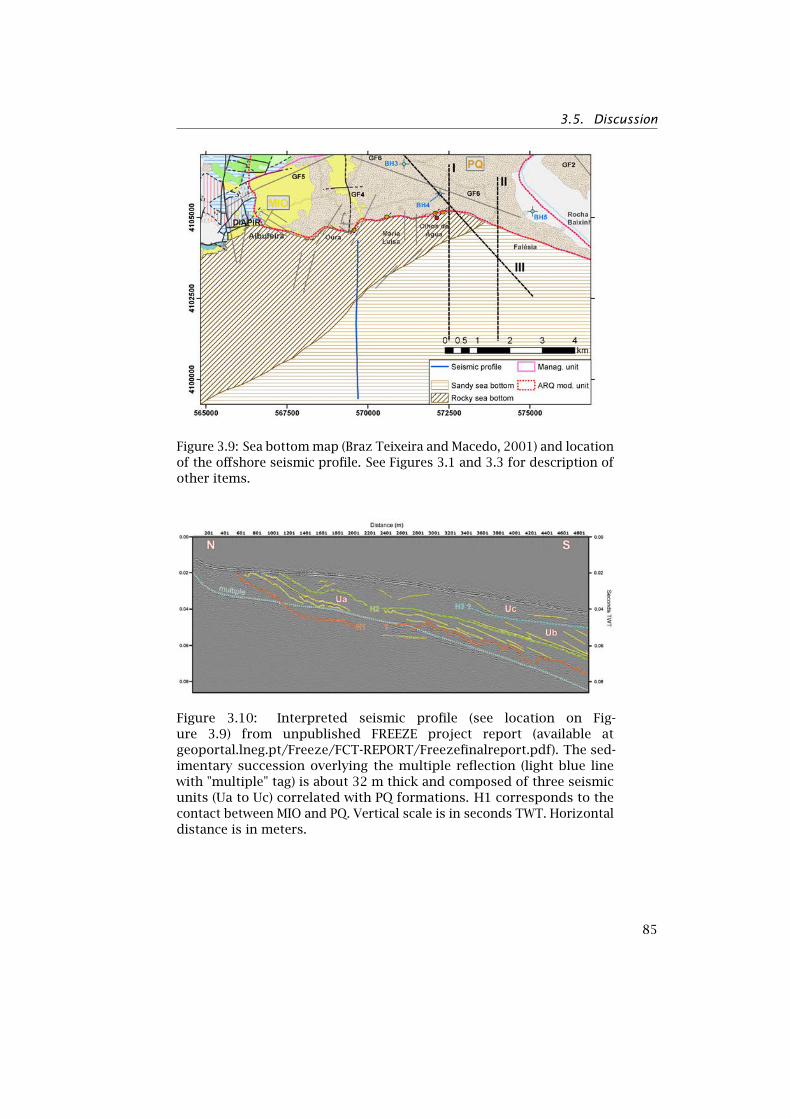
3.5. Discussion
Figure 3.9: Sea bottom map (Braz Teixeira and Macedo, 2001) and locationof the offshore seismic profile. See Figures 3.1 and 3.3 for description ofother items.
Figure 3.10: Interpreted seismic profile (see location on Fig-ure 3.9) from unpublished FREEZE project report (available atgeoportal.lneg.pt/Freeze/FCT-REPORT/Freezefinalreport.pdf). The sed-imentary succession overlying the multiple reflection (light blue linewith "multiple" tag) is about 32 m thick and composed of three seismicunits (Ua to Uc) correlated with PQ formations. H1 corresponds to thecontact between MIO and PQ. Vertical scale is in seconds TWT. Horizontaldistance is in meters.
85

3. Hydrogeological conceptual model of a coastal aquifer
Joining the geological and hydrogeological information described insection 3.2.2, the deductions made by the interpretation of the piezo-metric map and the hydrogeophysics, as well as offshore data previ-ously described and other (Lopes et al., 2006; Roque, 2007; Terrinhaet al., 2013), it was possible to conceive a 3D hydrogeological conceptualmodel. To illustrate it, 3 representative hydrogeological cross-sectionsare presented (Figure 3.11):
• cross-section I shows the case west of Olhos de Água, where the MIOis outcropping offshore, allowing the development of an outflowface characterized by inter- and subtidal groundwater springs. Itis probable that submarine groundwater spring extends to thewest of Olhos de Água between the coast and the boundary of theoutcropping offshore MIO. However, as these springs should bedeeper than the one at Olhos de Água, they should not be detectableat the sea surface;
• cross-section II shows the case at east of Olhos de Água, wherethe offshore PQ confines the offshore MIO and where no submar-ine groundwater springs are expected (only diffuse groundwaterdischarge, as represented by light blue arrows);
• cross-section III, oriented northeast-southwest, explains the con-centration of the inter- and subtidal springs at Olhos de Água.Considering that groundwater flow is towards south to southeastand the groundwater is trapped in the offshore confined MIO form-ations, the discharge must occur at Olhos de Água where the MIOaquifer still outcrops before disappearing below the PQ confiningunit.
This conceptual model was partially corroborated by an offshoresurvey of seawater electrical conductivity, temperature and depth (CTD)(Sousa et al., 2014). This CTD survey indicated that fresh submarinegroundwater discharges (SGD) occur in the proximal shelf between Albu-feira and Olhos de Água, mainly between -12 and -20 m, corroboratingthe case represented in cross-section I. East of Olhos de Água, i.e. wherethe MIO aquifer is confined by the PQ (cross-section II), no SGD weredetected by the CTD survey. The position of the FSWI will partially de-pend on hydraulic heads in the MIO and JUR aquifers, although still to besolved are the hydraulic relationships between the JUR and the MIO. It isprobable that as in onshore, the offshore JUR recharges the MIO, namelythrough fault zones. However the offshore geological settings is verycomplex, being also characterized by diapiric structures (Lopes et al.,2006; Roque, 2007; Terrinha et al., 2013) and there is a lack of data in theoffshore proximal shelf. Deep multichannel seismic reflection surveyswould be very valuable to clarify the relationships between offshore MIO,CRET and JUR.
The presented hydrogeological conceptual model indicates that theoffshore, confined MIO and JUR aquifers may store large groundwaterresources. Fresh groundwater resources trapped in offshore, confinedaquifer, have been identified in several coastal aquifers around the world
86

3.5. Discussion
Figure 3.11: Schematic cross-sections I to III (see location on Figure 3.3)representing the hydrogeological conceptual model. Vertical and hori-zontal scales are approximative. 87

3. Hydrogeological conceptual model of a coastal aquifer
(Post, 2005; Post et al., 2013). These authors proposed a paleoevolutionmodel of coastal aquifers to explain the occurrence of such hydrogeolo-gical configuration. This model is in agreement with the recent coastalshoreline paleoevolution in Algarve: the shoreline moved gradually frombathymetric -60 m up to its actual position during the transgressiveregime succeeding the Younger Dryas, in Upper Pleistocene (Dias et al.,2000). Several authors (Dias et al., 2000; Braz Teixeira and Macedo, 2001)detected submerged morphologies (abrasion platforms, cliffs and isth-mus) that were interpreted as paleoshorelines. The hydrography andhydrogeology of this period was similar to the actual ones, i.e. surfaceand groundwater were flowing towards south, with preferential path-ways of groundwater circulation until depths of about -40 m, and morerecently -20 m, where the beach springs would probably be located.
The 3D hydrogeological conceptual model of the ARQ aquifer, ex-tending ∼15 km offshore, was converted into 2D cross-sectional and3D variable-density groundwater flow numerical models (Hugman et al.,2014a). The objective of such numerical models was to test the hydraulicrelationships between JUR, CRET, MIO aquifers and seawater. Resultsconfirmed that SGD mostly occur at the offshore boundary between theMIO and the overlying low permeability PQ aquitard. Coastal freshwaterdischarges reached their maximum value in the area near Olhos de Água,being located up to 40 m away from the shoreline, which correspondsto field observations. The saltwater wedge in the MIO reached approx-imately 300 m inland. Depth and extent of the saltwater toe in the MIOwere similar to results from the FDEM cross-sections (Figure 3.6).
To reduce uncertainties in the groundwater numerical model, it wouldbe important to optimize the monitoring network, with at least one piezo-meter in each sector of the aquifer (unconfined JUR, unconfined MIO,confined JUR below CRET, confined JUR below MIO and CRET, confinedMIO below PQ). Groundwater level, electrical conductivity and temper-ature measurements could be automatically recorded at high temporalresolution (hourly or daily) with probes equipped with electronic sensorsand loggers at a relative low costs (∼1500 AC/sensor), only requiringdownloading of the data once or twice a year, depending on the memorycapacity of the logger. Such probes could be installed at low cost inthe deactivated municipality boreholes for which lithological logs andscreen depths are know. The spatio-temporal assessment of groundwa-ter recharge using existing hydrometeorological network of APA and adistributed recharge model coupled with a groundwater model (Monteiroet al., 2007b,a; Francés and Lubczynski, 2015) would also be relevant toconstrain the groundwater model. Such tools and data would largely be-nefit the groundwater management of the ARQ coastal aquifer, aiming topreserve the quality and quantity of the available groundwater resourcesthat frequently complement the water supply based on surface water.
88

3.6. Conclusion
3.6 Conclusion
A combination of geoelectrical and electromagnetic hydrogeophysicalmethods comprising TDEM, FDEM and ERT surveys were conductedonshore to clarify open questions related with the hydrogeological con-ceptual model of the ARQ coastal aquifer. Apart from useful resultsthat were obtained, limitations of the applied hydrogeophysical methodswere identified, which lead to proposals for further studies.
Two main modifications are proposed, leading to the definition ofa new ARQ modeling unit to be used in future efforts of groundwaterflow modeling. First, as the CRET was detected below the MIO layer inthe southern area of the ARQ, this aquitard should be included in thehydrogeological conceptual model as it controls the hydraulic connectionbetween the MIO and JUR. The multilayered nature of the system isof particular interest in a coastal aquifer due to the potential for anoffshore extent of fresh groundwater. Second, the western limit of theARQ management unit should be extended towards the Albufeira north-south fault (GF3), as there is geological and hydrogeological evidencethat the JUR layer extends south below the CRET, and that the GF5 faultdoes not constitute a hydraulic barrier. These two modifications arehighly relevant in the implementation of a groundwater flow model sincethe boundaries and defined hydrostratigraphical units have a strongimpact on the modeled water balance components and modeled aquiferhydrodynamics.
The shape of the FSWI was detected using the FDEM method, showinga steeper inclination in the western sector than in the eastern sector.This is explained by the higher hydraulic gradient in the west than in theeast. FDEM surveys perpendicular to the Quarteira stream, carried outduring different seasons, would help to clarify the hydraulic relationshipbetween this stream and the ARQ, in particular in the north sector.These two data, i.e. the shape of the FSWI and the influent/effluentcharacteristics of the Quarteira stream, are of use to constrain andcontrol the output of the groundwater flow model and would contributeto reducing uncertainty in simulated results.
The concentration of inter- and subtidal groundwater springs at Olhosde Água was explained taking into consideration the hydrostratigraphicalrelationships deduced by the hydrogeophysics and extending them tothe offshore proximal shelf taking into account other, complementaryoffshore studies. This conceptual model indicates probable groundwaterresources trapped offshore in the MIO layer confined by the PQ layer.
In a follow-up study (Hugman et al., 2014a), the upgraded hydro-geological conceptual model was implemented into a variable-densitygroundwater flow numerical model. It confirmed that coastal freshwaterdischarges are maximum at Olhos de Água and they mostly occur at theoffshore boundary between the MIO and the overlying low permeabilityPQ aquitard. The interchange of information between numerical model-ing and the hydrogeophysical-based conceptual models is an iterative
89

3. Hydrogeological conceptual model of a coastal aquifer
work towards less uncertain water balances and hydrodynamic aquifercharacterization. Together with the information derived from the nu-merical model and the recommendation of this study to complementthe hydrogeophysical survey, more data can be acquired to improve theknowledge of this complex aquifer system. The implementation of acoherent monitoring network of groundwater level and electrical con-ductivity may also contribute to a better understanding of the aquiferdynamics. The associated costs could be relatively low by making use ofexisting infrastructure. These several propositions would constitute asignificant improvement for the water management of the ARQ coastalaquifer, minimizing the risk of salinization and preserving a groundwaterresource that has been shown to be highly relevant in complementingor substituting the single source, surface water supply during droughtperiods.
90
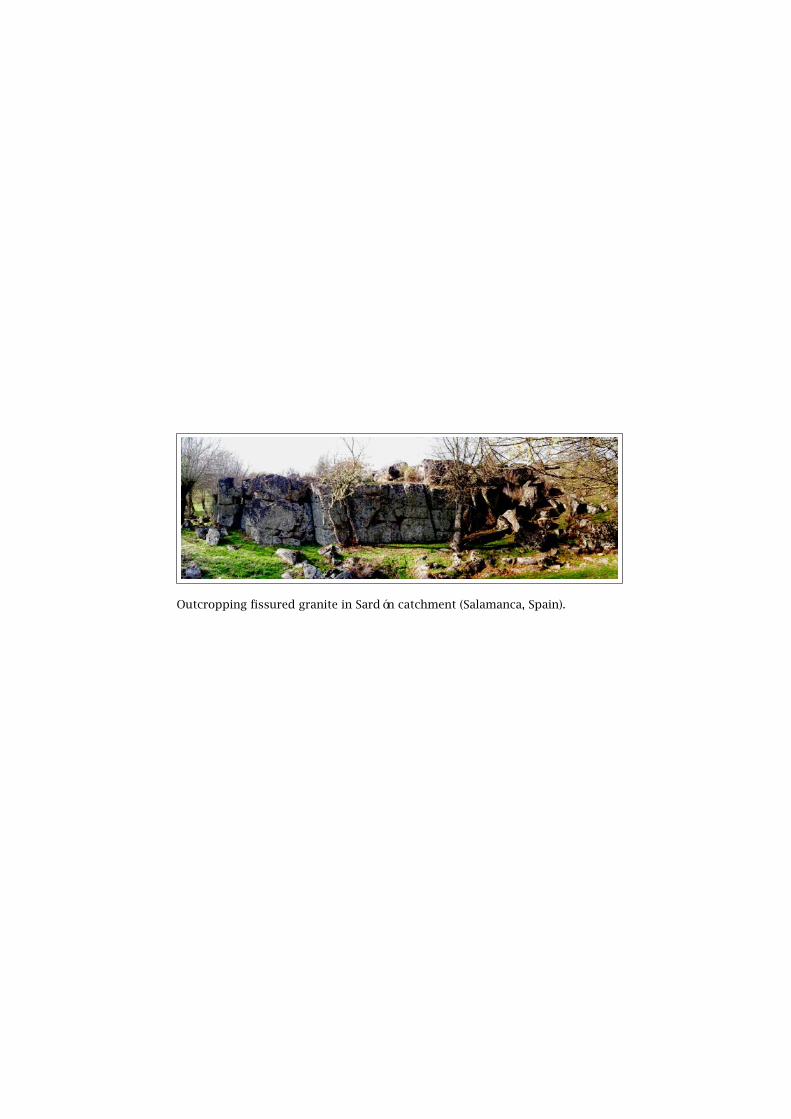
Outcropping fissured granite in Sardón catchment (Salamanca, Spain).


4Hydrogeophysics and remotesensing for the design ofhydrogeological conceptualmodels in hard rocks - Sardóncatchment (Spain)
4.1 Introduction
Although groundwater resources in hard rock aquifers are generallylimited in term of productivity, they are strategically important in manyregions of the world because they constitute a unique source of watersupply for population and agriculture (Cook, 2003; Singhal and Gupta,2010). Hard rock aquifers are characterized by high heterogeneity, whichleads to difficulties in groundwater prospecting, boreholes implement-ation and water resources management. This heterogeneity exhibit acomplex pattern that results from the interaction of factors such asmineralogy and texture of lithologies, regional and local tectonics, andpaleoclimate. An overall layout of the general conceptual model of hardrock aquifers, both from horizontal extent and depth-wise structure,was described by e.g. Lloyd (1999); Lachassagne et al. (2001); Dewandelet al. (2006). Its description includes from top to bottom: (i) an upperweathered layer, so-called saprolite, that has typically a storage function;(ii) an underlying fissured layer that has a transmissive function; and (iii)a fresh basement composed of massive, unaltered rocks with low primaryand secondary porosity. The mapping of such structures and retrievalof their hydraulic properties is essential to design a hydrogeologicalconceptual model of hard rock aquifers.
This chapter is based on: Hydrogeophysics and remote sensing for the design ofhydrogeological conceptual models in hard rocks Sardón catchment (Spain). Francés,A. P., M. W. Lubczynski, J. Roy, F. A. Monteiro Santos, and M. R. Mahmoudzadeh (2014),Journal of Applied Geophysics, 110, 63-81
93

4. Design of hydrogeological conceptual models in hard rocks
A hydrogeological conceptual model is a pictorial representation ofa groundwater flow system that summarizes available geological andhydrogeological information of a study area (Anderson and Woessner,1992). Its purpose is to help hydrogeologists to understand the behaviorof a hydrogeological system and to support quantitative modeling. Themore complex the geological setting, the more important is a hydrogeo-logical conceptual model. Therefore, particularly in hard rock aquifers,the design of a reliable hydrogeological conceptual model is a criticalstep in quantitative hydrogeological system assessment typically carriedout by groundwater modeling, as it strongly conditions the reliability ofsuch models.
Besides horizontal and depth-wise heterogeneities, another importantchallenge in hydrogeological studies of hard rocks is the scale depend-ence of aquifer parameters. Based on worldwide dataset of differentfractured rocks, Illman (2006) observed an asymptotic increase of per-meability from laboratory to regional scale. Sánchez-Vila et al. (1996),Neuman and Federico (2003) and de Marsily et al. (2005) presented atheoretical framework to explain this observation in different rock types.They pointed out the relevance of spatial organization and connectivityof low and high hydraulic conductivity (K) zones to explain the scaleeffect. Dewandel et al. (2012) studied the spatial distribution of aquiferparameters at the catchment scale in a deeply weathered crystallineaquifer in India (Maheswaram catchment). They observed that K was rel-atively homogeneous in the fissured zone at the scale of few hundreds ofmeters to around one kilometer. This observation is remarkable becausethis range is similar to the cell-size of numerical groundwater models atthe catchment scale.
The classical, physically based approach aims to analyze hydrologicalprocesses at the local scale and to scale-up the results to the catchmentscale (Sivapalan et al., 2003a). However, large scale preferential flowpaths in the subsurface may not be observed at the local scale, and thusmeasurement of properties at the local scale may be not adequate tomodel the catchment scale hydrodynamics. To account for heterogeneit-ies and scale dependence in hard rock aquifers, the concept of top-downapproach (Sivapalan et al., 2003b), also known as downward approach,is more adequate. The downward approach consists of analyzing thehydrology of a catchment by interpreting data obtained at the catchmentscale to find patterns in the observed data. It is inherently cross-scaleand multi-methods approach. Robinson et al. (2008) presented a reviewof electrical and magnetic geophysical methods to study the hydrologyof watersheds using the downward approach. As a general methodology,they proposed to use airborne electromagnetic system to identify thelarge-scale dominant structures and associated hydrological processes.The zones of interest were afterwards surveyed using ground-based,local geophysical methods. They also presented study cases in differentgeological settings where geophysics was used to identify the domin-ant hydrological processes and to quantify hydrological parameters orvariables.
94

4.1. Introduction
In hard rock aquifers, remote sensing (RS) techniques are frequentlyused to detect the main hydrogeological features at the catchment scale.Lineament detection based on digital terrain model (DTM) processingallows to identify the main fault zones, while geomorphological classi-fication supports the mapping of pediments (sub-horizontal hard rockerosion front), inselbergs and weathered areas (Srinivasa et al., 2000;Meijerink et al., 2007). Lachassagne et al. (2001) and Vouillamoz (2003)indicated RS and photo interpretation techniques as particularly suitableto obtain a first characterization of a study area to be subsequentlycomplemented at the local scale by geophysical methods. Additionally,Lachassagne et al. (2001) developed a downscaling methodology basedon GIS and multi-criteria analysis to map high-yield zones in the hardrock aquifer of Massif Central (France). The applied methodology integ-rated terrain parameters, such as lithology type, slope map, thickness ofweathered and fissured zones, fracture network information, obtained byRS and DTM analysis, conventional field work and geophysical surveys.
Subsurface data are generally scarce because invasive methods suchas borehole drilling and associated aquifer tests are expensive and time-consuming. Hydrogeophysics provides non-invasive, efficient methods ofsubsurface data acquisition to identify subsurface rock heterogeneitiesand potential high water yield zones in hard rock aquifers (Lloyd, 1999;Krishnamurthy et al., 2008). Each hydrogeophysical method has its owncharacteristics and capability with respect to aquifer characterization, sothe selection of the appropriate one must be done as a function of theobjectives of a survey and geological settings. Hydrogeophysical meth-ods such as geoelectric and electromagnetic have been widely used toretrieve hard rock hydrogeological structures (Dutta et al., 2006; Ramalhoet al., 2012) and aquifer parameters using empirical, area-specific rela-tionships (Chandra et al., 2008; Kirsch and Yaramanci, 2009). Amongthe hydrogeophysical methods, the magnetic resonance soundings (MRS)one has definite advantage for quantitative groundwater assessmentbecause of its most direct relation to in-situ subsurface water (Legchenkoet al., 2004; Lubczynski and Roy, 2007). Such direct relation is a resultof selective excitation of the water molecule’s hydrogen nuclei (1H+)and detection of its corresponding precession signal through nuclearmagnetic resonance (NMR). The 1D inversion of the measured MRS dataallows defining subsurface layers characterized by thickness, MRS watercontent and decay time constant. The application of the MRS output tosurface-based groundwater evaluation is detailed in several articles, suchas Roy and Lubczynski (2003), Plata and Rubio (2007) and Yaramanciand Hertrich (2009). In particular, the aquifer flow parameters, hydraulicconductivity (K) and transmissivity (T ), are derived from both MRS watercontent and decay time constant. The storage parameters, i.e. specificyield (Sy ) and elastic storativity (Se), are related with the MRS watercontent (Legchenko et al., 2004; Vouillamoz et al., 2005; Lubczynski andRoy, 2007; Vouillamoz et al., 2007), although recent studies also includedthe decay time constant (Vouillamoz et al., 2012b, 2014b,a). The MRSsensitivity of water detection was illustrated with a synthetic study of
95
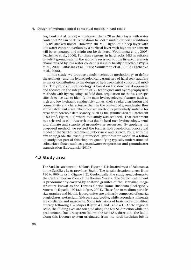
4. Design of hydrogeological conceptual models in hard rocks
Legchenko et al. (2006) who showed that a 20 m thick layer with watercontent of 2% can be detected down to ∼50 m under low noise conditions(∼5 nV stacked noise). However, the MRS signal of a deep layer withlow water content overlain by a surficial layer with high water contentwill be attenuated and might not be detected (Vouillamoz et al., 2005;Legchenko et al., 2006). For these reasons, in hard rocks, MRS is suitableto detect groundwater in the saprolite reservoir but the fissured reservoircharacterized by low water content is usually hardly detectable (Wynset al., 2004; Baltassat et al., 2005; Vouillamoz et al., 2005; Legchenkoet al., 2006).
In this study, we propose a multi-technique methodology to definethe geometry and the hydrogeological parameters of hard rock aquifersas major contribution to the design of hydrogeological conceptual mod-els. The proposed methodology is based on the downward approachand focuses on the integration of RS techniques and hydrogeophysicalmethods with hydrogeological field data acquisition methods. Our spe-cific objective was to identify the main hydrogeological features such ashigh and low hydraulic conductivity zones, their spatial distribution andconnectivity and characterize them in the context of groundwater flowat the catchment scale. The proposed method is particularly suitable forareas with borehole data scarcity, such as the granitic Sardón Catchment(∼80 km2, Figure 4.1) where this study was realized. That catchmentwas selected as pilot research area due to hard-rock hydrogeology, semi-arid climate and scarcity of groundwater resources. By applying theproposed method, we revised the former hydrogeological conceptualmodel of the Sardón catchment (Lubczynski and Gurwin, 2005) with theaim to upgrade the existing numerical groundwater model in a followup study (not part of this chapter), quantifying typically underestimatedsubsurface fluxes such as groundwater evaporation and groundwatertranspiration (Lubczynski, 2011).
4.2 Study area
The Sardón catchment (∼80 km2, Figure 4.1) is located west of Salamanca,in the Castilla y León province (Spain). The terrain elevation ranges from730 to 860 m a.s.l. (Figure 4.2). Geologically, the study area belongs tothe Central Iberian Zone of the Iberian Meseta. The Sardón catchmentis predominantly covered by anatexic granites of the Hercynian mega-structure known as the Tormes Gneiss Dome (Instituto Geológico yMinero de España, 1991a,b; López, 2004). These fine to medium particle-size granites and biotitic leucogranites are primarily composed of quartz,plagioclases, potassium feldspars and biotite, while secondary mineralsare cordierite and muscovite. Some intrusions of basic rocks (tonalites)outcrop following E-W stripes (Figure 4.1 and Table 4.1). At the regionalscale, the folding axes are oriented along the NW-SE direction while thepredominant fracture system follows the NNE-SSW direction. The faultsalong this fracture system originated from the tardi-hercinian brittle
96
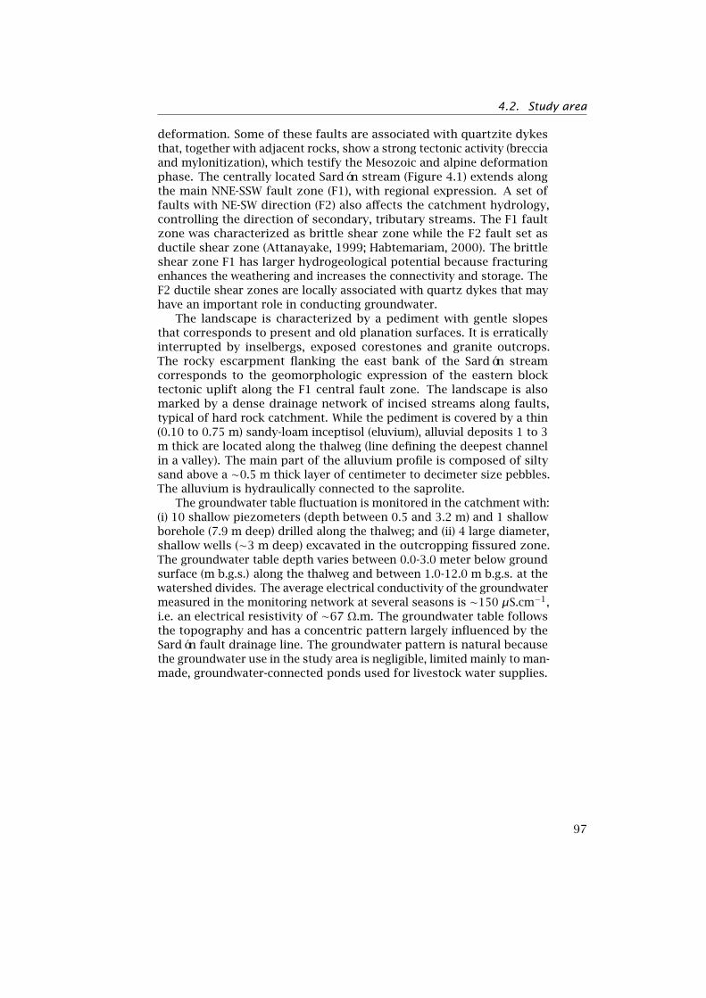
4.2. Study area
deformation. Some of these faults are associated with quartzite dykesthat, together with adjacent rocks, show a strong tectonic activity (brecciaand mylonitization), which testify the Mesozoic and alpine deformationphase. The centrally located Sardón stream (Figure 4.1) extends alongthe main NNE-SSW fault zone (F1), with regional expression. A set offaults with NE-SW direction (F2) also affects the catchment hydrology,controlling the direction of secondary, tributary streams. The F1 faultzone was characterized as brittle shear zone while the F2 fault set asductile shear zone (Attanayake, 1999; Habtemariam, 2000). The brittleshear zone F1 has larger hydrogeological potential because fracturingenhances the weathering and increases the connectivity and storage. TheF2 ductile shear zones are locally associated with quartz dykes that mayhave an important role in conducting groundwater.
The landscape is characterized by a pediment with gentle slopesthat corresponds to present and old planation surfaces. It is erraticallyinterrupted by inselbergs, exposed corestones and granite outcrops.The rocky escarpment flanking the east bank of the Sardón streamcorresponds to the geomorphologic expression of the eastern blocktectonic uplift along the F1 central fault zone. The landscape is alsomarked by a dense drainage network of incised streams along faults,typical of hard rock catchment. While the pediment is covered by a thin(0.10 to 0.75 m) sandy-loam inceptisol (eluvium), alluvial deposits 1 to 3m thick are located along the thalweg (line defining the deepest channelin a valley). The main part of the alluvium profile is composed of siltysand above a ∼0.5 m thick layer of centimeter to decimeter size pebbles.The alluvium is hydraulically connected to the saprolite.
The groundwater table fluctuation is monitored in the catchment with:(i) 10 shallow piezometers (depth between 0.5 and 3.2 m) and 1 shallowborehole (7.9 m deep) drilled along the thalweg; and (ii) 4 large diameter,shallow wells (∼3 m deep) excavated in the outcropping fissured zone.The groundwater table depth varies between 0.0-3.0 meter below groundsurface (m b.g.s.) along the thalweg and between 1.0-12.0 m b.g.s. at thewatershed divides. The average electrical conductivity of the groundwatermeasured in the monitoring network at several seasons is ∼150 µS.cm−1,i.e. an electrical resistivity of ∼67 Ω.m. The groundwater table followsthe topography and has a concentric pattern largely influenced by theSardón fault drainage line. The groundwater pattern is natural becausethe groundwater use in the study area is negligible, limited mainly to man-made, groundwater-connected ponds used for livestock water supplies.
97

4. Design of hydrogeological conceptual models in hard rocks
Figure 4.1: Geological map of the Sardón catchment (Villar Alonso et al.,2011) and geophysical surveys (red labels). Numbers of the geologicalformations refer to the original map and are explained in Table 4.1. F1and F2: main fault sets oriented NNE-SSW and NE-SW respectively.
98

4.2. Study area
Table 4.1: Geology of the Sardón catchment (Villar Alonso et al., 2011).
Group ID Description
Cenozoicrocks
156 Arkoses, conglomerates and pebbles (Eocene-Oligocene)
169 to184
Pebbles, gravels, sands and silts from terraces,depressions and endoreic areas, valley bottom,alluvium and colluvium, recent cones and fans,coluvium, and glacis (Pliocene to Holocene)
Paleozoicrocks (Ollo deSapo domain)
90 Schists, meta-arenites and calcium silicate rocks(Cambrien-Ordovician)
Prevariscanplutonicrocks
88 Feldspathic orthogneisses
Variscanplutonicrocks
10 Inhomogeneous granites
21 Two-mica granites
26 Intermediate and basic rocks (granodiorites andtonalites)
38, 39,46
Two-mica granites
Dikes 1 Quartz
3 Porphyritic granites and granodiorites
99

4.
Desig
nof
hyd
rogeo
logical
concep
tual
models
inhard
rock
s
Figure 4.2: Lineament detection and interpretation. a) DTM and fault set derived from high pass filter application on the DTM;b) first derivative in x; c) first derivative in y; d) gradient NE; e) gradient NW; f) gradient N; g) gradient W.
10
0

4.3. Methodology
4.3 Methodology
The proposed methodology is based on 3 steps: (1) detection of themain hydrogeological features of the catchment based on remote sens-ing (RS) techniques of digital image processing; (2) characterization ofthe main hydrogeological features at the local scale using qualitativeand quantitative hydrogeophysics; and (3) drilling of 5 boreholes (25 to48 m deep) and performing of slug tests to verify the hydrogeophysicalinterpretation and to calibrate the MRS parameters. The results from RSand hydrogeophysics were finally merged in a GIS environment, definingestimates for: spatial resolution, aquifer geometry, zones of hydrogeo-logical homogeneity together with the aquifers parameters distributionand range. This allowed designing the Sardón aquifer hydrogeologicalconceptual model.
4.3.1 Remote sensing techniques
Remote sensing (RS) techniques were applied to map: (i) fractures andfaults; and (ii) granite outcrops, using digital image processing on di-gital terrain model and high-resolution, multispectral satellite images.Fractures and faults were identified using lineament detection throughthe application of high-pass filters (Meijerink et al., 2007) on a DTM(Figure 4.2) of the Spanish Centro Nacional de Informacíon Geográfica(www.cnig.es) with 5 m horizontal resolution and centimetric verticalaccuracy that was validated in this study against differential GPS survey.High-pass filters highlight edges in images by calculating at each cell anew brightness value that is equal to the weighted average of the ori-ginal brightness value of the adjacent cells. Using the tools available inESRI®ArcGIS 10.0 for Desktop Advanced, we applied a kernel with format3×3 cells, applying the following weight matrices: first derivative in xand y directions and gradients in N, W, NW and NE directions. Based onthe resultant sharpened images, we digitized manually the lineaments.
Granite outcrops, i.e. the outcropping fissured layer, were mappedusing two high-resolution, multispectral satellite images: QuickBird fromSeptember 2009 and WorldView-2 from December 2012 (Figure 4.3). Bothimages were composed of 4 standard color bands, i.e. red, blue, greenand near-infrared, and had similar resolution (2.4 m for QuickBird and1.8 m for WorldView-2). A supervised classification technique based onobject-oriented fuzzy-logic analysis (Benz et al., 2004) using eCognitionsoftware was used to process the RS images in order to delineate fissuredlayer outcrops from the pediment. The description of this classificationtechnique, applied to soil mapping, is presented in Chapter 2 and Francésand Lubczynski (2011).
101
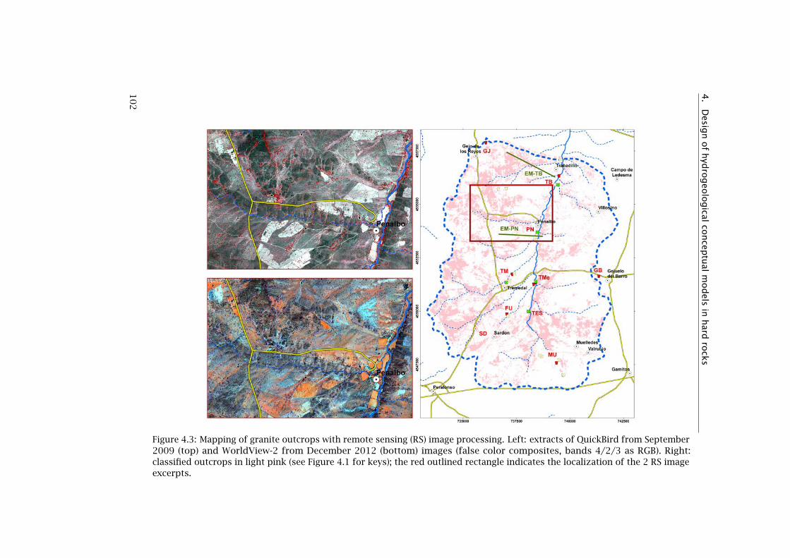
4.
Desig
nof
hyd
rogeo
logical
concep
tual
models
inhard
rock
s
Figure 4.3: Mapping of granite outcrops with remote sensing (RS) image processing. Left: extracts of QuickBird from September2009 (top) and WorldView-2 from December 2012 (bottom) images (false color composites, bands 4/2/3 as RGB). Right:classified outcrops in light pink (see Figure 4.1 for keys); the red outlined rectangle indicates the localization of the 2 RS imageexcerpts.
10
2

4.3. Methodology
4.3.2 Hydrogeophysics
The hydrogeological features detected in the previous step (fault zones,saprolite, fissured layer) were analyzed at the local scale using hydrogeo-physics. The locations of the surveyed sites were based on the followingcriteria: (i) to clearly belong to one of the representative hydrogeologicalfeatures mapped by RS; (ii) availability of ground truth subsurface in-formation such as lithology and depth of water table (piezometer, well,pond); (iii) accessibility to geophysical and drilling surveys.
4.3.2.1 Ground penetrating radar method
Ground penetrating radar (GPR) was applied to retrieve the spatial dis-tribution of groundwater table and soil thickness over the catchment(Mahmoudzadeh et al., 2012). A pulse radar with a single 200 MHz bowtieantenna was selected and combined with a differential GPS and a surveywheel for accurate positioning. The measurements were performed intransects transversal to stream beds, which were dry during the surveyperiod (September 2009). The acquired field data of the GPR reflectionwere interpreted by comparison with GPRMax2D forward modeling ofthe GPR signal with several hypothetical configurations of the subsurface,i.e. relative positions of soil, saprolite and groundwater table interfaces.The GPR data were locally transformed from time domain into depthby acquiring the soil dielectric constant with a frequency domain reflec-tometry probe (Seyfried et al., 2005). Details on that procedure can beobtained from Mahmoudzadeh et al. (2012).
4.3.2.2 Electrical method
In 2009 and 2010, we performed 16 electrical resistivity tomography(ERT) profiles (Figure 4.1) to retrieve the hydrostratigraphy and detectvertical heterogeneities. The ERT method is described in details in severaltextbooks as for instance Ernstson et al. (2009). We used a programmable,commercial resistivity-meter Supersting R8 from Advanced GeosciencesInc. (AGI). This 8-channel instrument was equipped with a central switchbox and 4 passive cables, each one with 14 electrodes (56 electrodes intotal) and maximum basic electrode spacing of 6.25 m. We programmedtwo single spread Schlumberger arrays (i.e. without roll-along config-uration), each one with basic electrode spacing of 3 and 5 m. The A-Bcurrent electrodes separation ranged from 9 to 162 m for the 3 m basicelectrode spacing and from 15 to 270 m for the 5 m basic electrodespacing.
Due to the overall project logistics, the field surveys were done dur-ing the end of the dry period in September and October. Although thisperiod was favorable to obtain the highest resistivity contrast betweenunsaturated and saturated zones, the topsoil was very dry which resultedin frequent high contact resistances (>5000 Ω). Not much improvementwas obtained by pouring salty water at each electrode due to the low
103

4. Design of hydrogeological conceptual models in hard rocks
water content of the soil and significant thickness of the very dry un-saturated layer. The poured water was absorbed by the soil around theelectrode, creating a bigger soil electrode, but with no contact with thesignificant soil moisture content located much deeper (Lloyd, 1999). Sim-ilar problem was encountered by Danielsen et al. (2007) that had galvaniccontact problems in Kalahari sands, even while watering and using 0.5-1 m long electrodes. In our case, we filtered the dataset before inversionby removing the data with high contact resistance using the "Exterminatebad datum points" option of the RES2DINV software (Geotomo software,2010). When the number of removed electrodes was too high (i.e. >1/3of the full dataset), the inversion was not performed. Otherwise, theinversion was performed following the recommendations for noisy dataas specified in the RES2DINV manual (Geotomo software, 2010). Weapplied the robust method of the RES2DINV software because sharpboundaries between the unsaturated and saturated zone and betweenweathered, fissured and fresh granite were expected. After the firstinversion, all points with root-mean-squared error between calculatedand measured apparent resistivities higher than 50% were removed andthe final inversion was performed to obtain a vertical cross-section ofthe electrical resistivity.
To retrieve the hydro-layering of the saprolite and the fissured lay-ers based on the obtained resistivity cross-sections, we interpreted theresistivity contrasts in subsurface. Based on the surface geology know-ledge (field observation, geological map and remote sensing mapping),we defined range of resistivity characteristics of the saprolite and thefissured layer.
4.3.2.3 Electromagnetic method
One of the specific objectives of this study was to map the spatial anddepth-wise extension of saprolite, fissured layer and fault zones. Forthat purpose, we required an efficient method that would allow detectingvertical and horizontal subsurface resistivity contrasts across the catch-ment. Time domain electromagnetic (TDEM) systems are frequently usedto determine the subsurface geoelectrical 1D profiles. There are howeverpractical limitations in the use of such configurations at shallow depthsand where high lateral resolution is expected (Christiansen et al., 2009).Instead, for such tasks, electromagnetic systems using dipolar sourcesand normally operated in the frequency domain (FDEM) have been used.One well-known implementation of an electromagnetic system designedfor high resolution shallow work is the electromagnetic conductivitymeter (McNeill, 1980). Detailed surveys using this type of instrument arereported for the mapping of near surface conductivity changes with highspatial resolution (Triantafilis and Monteiro Santos, 2010; Francés andLubczynski, 2011). Electromagnetic conductivity meter data providesinformation on the lateral changes in conductivity but its soundingcapability (i.e. vertical distribution of conductivities) is limited.
In this study, we used a multi-frequency electromagnetic horizontal
104

4.3. Methodology
coplanar loop system (Slingram). The 1D soundings were performed at aregular distance along transects, using several coil distances. Such deviceand configuration allowed us to determine the vertical distribution ofresistivity below the ground surface while at the same time, as data wereacquired along transects, the lateral changes were also detectable. Theselected device was Apex Parametrics Ltd. MAX-MIN I8S equipment with8 frequencies from 444 Hz to 56 kHz. This device measured at eachfrequency the quadrature and in-phase components of the secondaryelectromagnetic field. To ensure high quality data, a rigid frame wasused for operation of the Slingram electromagnetic set with short 5 mcoil spacing to minimize the difficulties in maintaining a constant inter-coil coupling (distance and orientation) in the coplanar configuration(Parasnis, 1966).
The dataset of 1D FDEM soundings along the transects was processedusing a laterally constrained inversion (LCI) algorithm (Monteiro Santos,2004) to obtain subsurface resistivity cross-sections. The LCI algorithmis a modified 1D inversion with 2D smoothness constraints betweenadjacent 1D models, i.e. the inverted value in each cell is computedtaking into account the measured values in the 4 adjacent cells (top,bottom, right, left). Electromagnetic forward and derivative calculationswere performed using the full solution of the Maxwell equations (Kellerand Frischknecht, 1966). Based on the inversion of the quadrature andthe in-phase components of the MAX-MIN data, the algorithm retrievesthe electrical resistivity cross-section. The quality of the inversion isassessed by the quality of the fit between the observed and simulatedcurves of in-phase and out-phase. The two FDEM transects (Figure 4.1),one at the latitude of Peñalbo (EM-PN) and another at the latitude ofTrabadillo (EM-TB), were realized in November 1996. The EM-PN wasperformed with both 5 m (rigid frame) and 120 m coil separations whilethe EM-TB only with 120 m coil separation. For both transects, the datawere acquired every 60 m.
4.3.2.4 Magnetic resonance sounding method
We performed 15 MRS surveys organized in 3 campaigns in years 1997,2001 and 2009 (Table 4.2 and Figure 4.1), aiming to define hydrostrati-graphy and aquifer parameters. In all the campaigns and at every siteinvestigated, the measurement of the Earth magnetic field (B) was car-ried out with a magnetometer just before and during the MRS survey tocalculate the Larmor frequency (fl). In the 2001 campaign, it turned outthat the local value of the Earth’s magnetic field expressed as Larmorfrequency was very near 1900 Hz, i.e. one of the 50 Hz power line fre-quency harmonics, which resulted in very noisy, non-interpretable signalin most of the surveys of that year. As explained in Bernard (2007), floutside the 50 Hz harmonics and local scale magnetic homogeneity arerequired to successfully acquire magnetic resonance signal. Thus, tominimize the risk of unsuccessful MRS data acquisition during the 2009campaign, one month before the MRS surveys, we measured the natural
105

4. Design of hydrogeological conceptual models in hard rocks
Table 4.2: Summary of the three MRS campaigns.
Camp. Equip. Performed Successful
Numberof MRS
Sites Numberof MRS
Sites Loop
1st -1997
NUMIS 3 TB, PN,TM
3 TB, PN,TM
40 m square
2nd -2001
NUMIS 4 MU, TES,TB
1 TES 56 msquare-eight
3rd -2009
NUMISLITE 8 FU, MU,PN, TB,TMe
2 TMe 30 msquare-eight,60 m square
Earth magnetic field (B) and its spatial variability to detect potential localscale magnetic inhomogeneity and to ensure that fl was outside the50 Hz harmonics. The spatial magnetic field measurements were madeusing a magnetometer Geometrics G856 as rover and the temporal meas-urements were acquired every minute with a Geometrics G816 as base.The values of the magnetic field measured with the rover were correctedfrom the diurnal drift measured with the base magnetometer, using thesoftware Geometrics MagMap2000. To locate the measurements we useda standard GPS with synchronized time between the rover and the baseto allow the correction. At each selected site, 36 magnetometric meas-urements were carried out within 100×100 m rhomboid area. In totalwe made 629 measurements distributed over 20 sites. B showed to bequite homogeneous, with a mean of 44805 nT, small standard deviationof 7 nT and difference between maximum and minimum values of 34 nT.The corresponding fl was 1908 Hz, i.e. outside the problematic intervalsof the 50 Hz of electrical power line harmonics. We also measured themagnetic susceptibility of granite outcrops and soils at 6 sites (GB, PN,TM, MU, TMe, FU in Figure 4.1) using a SM-20 device from GF Instruments.The magnetic susceptibility measured on 37 outcrops and soils wasless than 10−3 SI (average of 0.06×10⁻³ with minimum and maximum0.01×10−3 and 0.2×10⁻³ respectively), so suitable for MRS surveys.
In the first and the second MRS campaigns (1997 & 2001, Table 4.2),we used the original NUMIS version (Iris Instrument) equipment with asingle DC/DC converter and the evolving version of its NUM data acquisi-tion software. At that time, using the equipment and software availablefor this project, MRS was implemented in a single pulse mode allowingdetection and measurement of the signal from free induction decay (FID).The data processing at acquisition time yielded the signal amplitude(E0) and the FID time constant (T∗2 ). Following a data inversion step, theMRS data set yielded two aquifer related parameters as a function ofdepth: MRS free water content (θMRS ) and T∗2 . T∗2 is dependent on: (i) thetransversal decay time constant (T2), itself dependent on the sampled
106

4.3. Methodology
volume petrophysical properties such as pores-size; (ii) inhomogeneityof the ambient magnetic field (Fukushima and Roeder, 1981):
1/T∗2 = 1/T2 + γ∆B0 (4.1)
where γ is the gyromagnetic ratio and ∆B0 is the ambient magneticfield inhomogeneity typically caused by the 3D spatial distribution ofmaterials ranging in scale from geological structure, such as dyke, downto fine-grain minerals with significant magnetic susceptibility higherthan background. In contrast to T∗2 , the longitudinal decay time constant(T1) is not sensitive to local inhomogeneity of the Earth magnetic fieldB, so it is more reliable than T∗2 for pore size estimation and relatedhydrogeological system parameterization (Legchenko et al., 2004; Royand Lubczynski, 2005; Vouillamoz et al., 2007). For the 2009 campaign(Table 4.2), we used the newer NUMISLITE equipment together with itsdata acquisition software Prodiviner which, although less powerful thanthe original NUMIS, allowed more complex data acquisition modes. Inparticular, this MRS system allows estimating T1 using a modified nuclearmagnetic resonance (NMR) saturation recovery scheme Legchenko et al.(2004). More recently, Legchenko (2013) reviewed different ways ofexploiting NMR for MRS purposes. All three data sets of the three MRScampaigns (Table 4.2) were then processed with the version 11.3 ofthe Samovar software tool (Legchenko, 2011), applying its "complexamplitude mode", to ensure consistency among the inversion results ofthe three different campaigns. The geoelectrical models supporting theMRS inversions were built using the ERT cross-sections, complementedin some cases with 1D inversion of TDEM data acquired with a TEM-FAST48 from Applied Electromagnetic Research (50 m loop).
To retrieve the flow parameters from the MRS data, we used thefollowing relationship (Lubczynski and Roy, 2007; Vouillamoz et al.,2007):
TMRS = CTn∑i=1
∆ZMRSiθMRSiT1i2 (4.2)
KMRS = TMRS/n∑i=1
∆ZMRSi (4.3)
where TMRS is the transmissivity (m2.s−1), KMRS is the MRS hydraulicconductivity (m.s−1), ∆ZMRSi, θMRSi and T1i are thickness (m), free watercontent (m3.m−3) and longitudinal decay time constant (ms) of each waterbearing layer retrieved by the MRS inversion (i is the index of a layer andn is the total number of layers) respectively, and CT is an area-specific,empirical transmissivity multiplier that can be computed at sites whereboth aquifer tests and MRS surveys are available.
As T1 was not acquired in the first two campaigns of 1997 and 2001,we used the measurements of the 2009 campaign with measurements
107

4. Design of hydrogeological conceptual models in hard rocks
of both T1 and T∗2 to derive the ratio DT = T1/T∗2 , considered repres-entative for the granitic Sardón area. In practice, we reviewed all 2009measurements and eliminated extreme, unreliable T∗2 by selecting onlyinversion results that ensured the following arbitrary conditions:
50 < T∗2 < 750 ms and θMRS > 1.5% and T1 > T∗2 (4.4)
Finally, we used the ratio DT to compute backward T1 using T∗2measurements acquired during the 1997 and 2001 surveys.
Slug tests were performed in the drilled boreholes (Figure 4.1 andnext section) to derive the transmissivity (TST ) and then CT followingEquation (4.5) (Vouillamoz et al., 2005, 2007):
CT = TST/n∑i=1
∆ZMRSiθMRSiT1i2 (4.5)
The relationship between MRS parameters and groundwater storageparameters is still not well established (Vouillamoz et al., 2012b). Thecomputing of extractable groundwater storage in unconfined aquifersrequires the specific yield (Sy ) while in confined aquifers the elastic stor-ativity (Se). The MRS survey provides θMRS , which is an estimate of thefree water content (θf ) that is composed of both extractable, gravitationalwater and immobile, non-extractable capillary water (Lubczynski andRoy, 2007). Thus neither Sy nor Se are equivalent to θMRS although thereare empirical relations between them (Lubczynski and Roy, 2004, 2007;Vouillamoz et al., 2007; Boucher et al., 2009b; Vouillamoz et al., 2012b).In this study, to calculate unconfined and confined storage parameterswe used the empirical Equations (4.6) and (4.7) respectively (Vouillamozet al., 2007):
SyMRS = CyθMRS (4.6)
SeMRS = ρwg∆ZMRS(α+ βθMRS) = Ce(θMRS∆ZMRS) (4.7)
where SyMRS is the MRS specific yield, SeMRS is the MRS elastic storativ-ity, Cy and Ce are empirical storage multipliers of the specific yield andelastic storativity respectively, ρw is water density, g is gravitationalacceleration and α and β are aquifer and water compressibilities respect-ively. Cy and Ce estimates derived in granites of Burkina Faso and inother lithological formations are available in Vouillamoz et al. (2005) andVouillamoz et al. (2007).
4.3.2.5 Boreholes drilling and slug tests
The borehole drilling sites were selected following the geological contextand when possible by using the interpretations of the ERT and FDEM,aiming to intersect either the saprolite or the fissured layer. At some
108
4.4. Results and discussion
sites, it was not possible to drill due to land owner restrictions. In total,we could drill 5 boreholes down to depths ranging from 25 to 48 m at 4sites (TB, PN, 2×TMe, SD, Figure 4.1) with the following objectives: (i) toconfirm the hydrostratigraphy derived from hydrogeophysical surveys;(ii) to analyze the hydraulic connection between saprolite and fissuredzone; (iii) to perform aquifer tests to compute the aquifer parametersand calibrate the MRS parameters. The borehole at PN (24 m deep) andthe two at TMe (38 and 42 m deep) were drilled in heavily weatheredgranite (saprolite). They showed very small yield <0.1 l.s−1. Anotherborehole at the TB site was intended to intersect the saprolite followingthe interpretation of the ERT cross-section. However, as we could notdrill exactly at the intended location due to the land owner restriction, theborehole intersected fissured granite already at 3 m b.g.s. and continueddown to 40 m b.g.s. (total depth of the borehole). At the last, fifth SD site,the borehole was intentionally drilled in fissured granite and extendeddown to 48 m b.g.s. Both TB and SD boreholes intersected small fractureswhich produced total yields between 0.1 and 0.3 l.s−1.
Due to the generally low borehole yield, in all 5 boreholes, we per-formed slug tests instead of pumping tests (Butler and Healey, 1998).Slug tests allow determining efficiently the hydraulic conductivity butare generally considered to be only representative of a small volume ofaquifer material around the well and do not provide storage properties.Slug tests were interpreted with the Rice-Bouwer method (Kruseman andde Ridder, 1991) using programmed spreadsheets of Tonder et al. (2002).
4.4 Results and discussion
4.4.1 Aquifer geometry
4.4.1.1 Lineament mapping
The images obtained by the application of high-pass filters on the highresolution digital terrain model (DTM) from the Centro Nacional deInformacíon Geográfica are presented in Figure 4.2. The images of Fig-ures 4.2b-g highlight clearly the lineaments that were manually digitizedand interpreted as presented in Figure 4.2a. By using high-pass filtersover DTM, the linear contrasts in terrain elevation of adjacent cells wereenhanced. The obtained lineaments corresponded explicitly to geologicaland geomorphological features (e.g. lithological boundaries and faults).In contrast, optical satellite images or aerial photography also incorpor-ate man-made, linear infrastructures, such as roads or fences. As thesestructures have a different brightness than surrounding terrain, they areenhanced by high-pass filters, being mapped as lineaments, so poten-tially misinterpreted as natural geological features. This is why previousattempts, performed using LANDSAT TM and aerial photography (At-tanayake, 1999), were less satisfactory than the current results obtainedwith the DTM.
109

4. Design of hydrogeological conceptual models in hard rocks
In Sardón study area, fractures are mainly oriented in the NE-SWdirection (F2 fault set), being connected to the central fault zone orientedNNE-SSW (F1 fault zone). A third fault set (F3), oriented E-W is alsoconnected to the F1 fault zone. We also identified a fourth and fifth setsof fractures in the directions NW-SE (F4) and NNW-SSE (F5) respectively.However, only the F1 fault zone and the F2/F3 fault sets showed a closerelationship with the stream network, being therefore responsible forgroundwater drainage of the catchment. These results are in agreementwith field observations made by Habtemariam (2000) and with the lin-eament analysis at the regional scale made by López (2004) who foundthat the stream network was mainly associated with faults of directionbetween N10°E and N50°E.
4.4.1.2 Horizontal extent of saprolite and fissured layers
The horizontal extent of the granite outcrops that was mapped using asupervised classification method applied on high-resolution remote sens-ing images is presented in Figure 4.3. The outcrops were associated withthe fissured layer while the non-outcrops with saprolite. The classifica-tion method used in this study with two high resolution, multispectralsatellite images improved the outcrop mapping presented in Lubczynskiand Gurwin (2005) that was done by manual digitizing on stereoscopicaerial photographs. The improvements were mainly due to the availab-ility of near-infrared band and combination of two images, one fromdry and the other from wet periods (Figure 4.3 left-top and left-bottomrespectively), which allowed enhancing the color contrasts between landcover features. The applied technique showed to be repeatable, fasterand more accurate than the former manual interpretation.
4.4.1.3 Water table depth
The 5 boreholes drilled in this study allowed to complement the informa-tion provided by the monitoring network mainly restricted to the shallowalluvium and saprolite along the central Sardón stream. Boreholes drilledin the saprolite at PN and TMe confirmed the presence of shallow, uncon-fined water table at ∼2 m depth. The boreholes drilled directly in fissuredgranite at TB and SD sites intersected productive, confined fissures at∼20 m depth with water table stabilized at ∼2 m depth, i.e. at similardepth as the water table in the saprolite. This indicated that the fissuredlayer is hydraulically connected with the saprolite layer.
To extend the groundwater table depth information available frompiezometers, wells and groundwater-linked ponds to areas not coveredby the observation network, Mahmoudzadeh et al. (2012) applied GPRtechnique along number of transects. Using forward modeling of the GPRsignal, they demonstrated that the groundwater table interface returnsa strong microwave reflection signal. Less visible in the presence ofshallower water table was the contact between the soil (either alluvium<2 m thick or eluvium <1 m thick) and the saprolite. Comparing these
110

4.4. Results and discussion
forward modeling results with the GPR field data, it was evidenced thatthe water table was present in both alluvium and eluvium and that itfollowed the topography. In the shallow or outcropping fissured zones,the GPR detection of the water table in discrete, thin fracture zones wasnot possible due to multiple ambiguous reflections of the GPR signal. Thedepth assessment of both water table and eluvium/saprolite interfacewas uncertain because the time-depth transformation was done usinga single, bulk dielectric constant value. At sites where both GPR dataand water table depth measurements were available, the value of thedielectric constant was calibrated, which allowed to estimate the watertable occurring at the depth of ∼1-3 m b.g.s.
The ERT and FDEM methods were not able to detect accurately thewater table depth. In this study the applied methods were optimizedto retrieve the aquifer layering, i.e. the measurements were made withelectrodes and coil separations at the multi-meter scale while the depthresolution requirement for the groundwater models was at the centimeteror at least decimeter scale.
The MRS method has the capability to assess the water table depth inhard rock aquifers (Wyns et al., 2004; Legchenko et al., 2004; Vouillamozet al., 2005; Legchenko et al., 2006), but only if the aquifer water contentis above the technique’s sensitivity threshold. New, smaller MRS instru-mentation (Walsh et al., 2014) optimized to water table depth detection inthe shallow (<30 m) subsurface may successfully contribute to mappingof the water table depth, keeping in mind the water content sensitivitythreshold of such instruments.
4.4.1.4 Hydrostratigraphy of saprolite and fissured layers
Electrical resistivity tomography profiles
Out of the 16 electrical resistivity tomography (ERT) profiles per-formed (Figure 4.1), we could only invert and interpret 8 that resulted inthe resistivity cross-sections presented in Figure 4.4. The 2D resistivitycross-sections ranged from 165 to 275 m length and extended from 20to 45 m b.g.s., depending on whether the profiles were implemented with3 or 5 m electrode separation. The root-mean-squared error betweenthe calculated and measured apparent resistivity values, as indicated inFigure 4.4, was between 2.6% at TB and 12.6% at TM.
The TMe and TB cross-sections were carried out across the main cent-ral F1 fault zone (Figure 4.1). At TMe, two ERT profiles were performed,TMe(NE) and TMe(SW). As shown in Figure 4.4, the two cross-sectionsshow in their western and central part a conductive layer with resistivitybetween 5 and 75 Ω.m extending down to ∼40 m b.g.s. and overlain bya thin, resistive unsaturated zone. That layer is interpreted as heavilyweathered granite (saprolite layer). In both TMe, the saprolite layer isunderlain by more resistive layer of 150-200 Ω.m interpreted as fissuredzone granite. The main difference between the two TMe is observed intheir eastern sections. In contrast to TMe(SW), the TMe(NE), located more
111

4. Design of hydrogeological conceptual models in hard rocks
Figure 4.4: Inverted electrical resistivity cross-sections of ERT data (seelocation in Figure 4.1). Circles indicate the position of the inversion cells.RMSE is the root-mean-squared error, expressed in percent, between thecalculated and measured apparent resistivity values.
112

4.4. Results and discussion
– continued from previous page
to the east, intersects granite outcrop at the eastern margin of the F1 faultzone. This is marked by generally larger resistivity of shallow fissuredgranite extending down to ∼15 m b.g.s. with resistivity ∼500 Ω.m andunaltered fresh granite underneath with resistivity >1000 Ω.m, sharplybordering with saprolite along the eastern edge of the F1 fault zone. Inthe TB cross-section, the saprolite layer identified with resistivity between50 and 100 Ω.m extends below the bottom of the inverted resistivitycross-section. At its SE side, the higher resistivity block (150-200 Ω.m)corresponds to fissured granite, as observed on outcrops. The TM cross-section carried across the F2 fault shows a saprolite layer with resistivitybetween 5 and 50 Ω.m and a thickness of ∼35 m. Like in TMe along F1fault zone, the saprolite layer is underlain by fissured zone with similarresistivity but occurring at shallower depth of 25-35 m b.g.s. Like TM,the FU cross-section was made across the discontinuity depicted by RSand field investigation as F2 fault. The F2 fault zone is at the NW side ofthe cross-section and is less pronounced than in TM cross-section. Thecentral part of the FU cross-section is occupied by resistivity between100 and 500 Ω.m, which corresponds to the fissured zone. Finally, thecross-sections GJ, GB and MU located at the top of the hills, far fromthe fault zones, show a layer 10 to 20 m thick with resistivity between150 and 750 Ω.m, indicating the fissured zone and absence of saprolite.Note that at these 3 sites the presence of groundwater was confirmed in
113
4. Design of hydrogeological conceptual models in hard rocks
shallow dug wells belonging to local farmers. These wells contain waterall year long and recover after pumping. They however show a low yieldand are not used for farming activities.
The use of ERT in the Sardón catchment area allowed to depict qual-itatively and to certain extent also quantitatively the thickness and ho-rizontal extent of the saprolite and fissured layers. Within this project,our ERT profiles with single spread Schlumberger configuration of 56electrodes yielded limited profile length and depth reach. In particular,the ERT profiles did not characterize the bottom part of the F1-relateddeep saprolite zone. Another caveat is the use of electrical method insemi-arid to arid environment. The dryness of the topsoil layer resul-ted in very high contact resistance that made difficult data acquisitionand decreased ERT data quality. In the wet season, more reliable signalcan be acquired in areas within valley bottoms due to the presence ofclay-enriched thick and conductive top soils. However, along the graniticslopes covered by sandy-loam eluvium with poor clay content, ensuringan adequate electrode contact resistance can remain a challenge.
Frequency domain electromagnetic transects
The two frequency domain electromagnetic (FDEM) transects EM-PN(Figure 4.5a) and EM-TB (Figure 4.5b) with lengths 1620 m and 2160 mrespectively, are transversal with respect to the main Sardón valley(Figure 4.1). The two FDEM inverted electrical resistivity cross-sections(Figure 4.5) showed a similar depth extension (∼50 m b.g.s.) as comparedto the ERT cross-sections. In the FDEM data inversions we did not usethe lowest frequency of 444 Hz due to incoherent values. In generalthe goodness of fit between observed and simulated values was good,having the largest discrepancy at high frequency (shallow subsurface),which may be due to the strong contrast between high resistivity of thedry unsaturated zone and low resistivity of the saturated alluvium orsaprolite.
The EM-PN cross-section (Figure 4.5a) crosses the F1 fault zonebetween 850 and 1450 m, along the main Sardón valley. The F1 faultzone shows a surficial, ∼10 m thick lens of very low resistivity material(1 to 15 Ω.m) that corresponds to clayey deposits (alluvium or heavilyweathered granite). This clay deposit was observed south of Peñalbovillage by drilling down to 6 m depth (without reaching bottom of thatclay layer) with a portable gasoline powered percussion hammer. Belowthe clay, there is a zone of low to moderate resistivity (15 to 100 Ω.m),likely corresponding to saprolite. East of the F1 fault zone, the highresistivity block (>500 Ω.m) corresponds to the outcropping fissuredgranite of the eastern block, uplifted along the F1 fault observed in thefield in the form of escarpment and also by the RS images (Figure 4.3).The same, high resistivity block is also defined by ERT cross-sectionTMe(NE) in Figure 4.4. West of the F1 fault zone between 0 and 600 m,the outcropping fissured granite is characterized by large resistivities
114

4.4. Results and discussion
Figure 4.5: Inverted electrical resistivity cross-sections of FDEM data (seelocation in Figure 4.1): a) EM-PN; b) EM-TB. Circles indicate the positionof the inversion cells.
>1000 Ω.m which is in agreement with the outcrop mapping presentedin Figure 4.3.
The EM-TB transect (Figure 4.5b) is located in the northern part of theSardón catchment. In its SE limit, it reaches the western extent of theF1 fault zone that shows the same resistivity characteristics as in theEM-PN cross-section. To the west of the F1 fault zone, i.e. between 900and 2000 m, 3 layers can be clearly identified from top to bottom: (i) a∼10 m thick, surficial layer with very high resistivity of ∼1000 Ω.m; (ii)a ∼20 m thick sub-horizontal layer with resistivity from 30 to 75 Ω.m;and (iii) a high resistivity layer (250-750 Ω.m). These three layers likelycorrespond respectively to unsaturated and saturated sections of thesaprolite underlain by fissured granite. Between 600 and 900 m, alow resistivity layer (30-75 Ω.m) sloping towards NW separates highresistive layers (>1000 Ω.m) from above and below. That layer likelycorresponds to the extension in depth of the outcropping tonalite dikevisible in Figure 4.1, while the resistive, overlying layer corresponds tooutcropping granite (see also Figures 4.1 and Figure 4.3).
The results of the 2 FDEM cross-sections are coherent with the ERTresults and with the general geological knowledge synthetized in Fig-ure 4.1. The FDEM method was very efficient, allowing to cover largedistance in short time as for example it took only ∼5 h to measure theresistivity data with 5 m coil separation along the EM-PN transect (1620 m
115

4. Design of hydrogeological conceptual models in hard rocks
long, data acquired every 60 m). Although the spatial resolution of dataacquisition was quite coarse - every 60 m - it was sufficient to identify themain geological features such as the F1 fault zone and the resistivity con-trast between saprolite and fissured layers. We thus highly recommendthis method for the hydrostratigraphy assessment in hydrogeologicalprospecting of hard rock areas.
Magnetic resonance soundings
Out of the 15 magnetic resonance sounding (MRS) surveys performedin 3 different campaigns (Table 4.2), we obtained only 6 interpretableMRS surveys at 5 sites (Figure 4.1) with signal to noise ratio (S/N) between2 and 9 (Figure 4.6). Among them 5 were located along the central F1fault zone (1 at TB, 1 at PN, 2 at TMe and 1 at TES) and 1 along a F2 faultzone (TM). The first 3 columns from the left of Figure 4.6 present theMRS data acquired in the field while the 4th and 5th columns representthe inverted depth-wise variability of the MRS free water content (θMRS )and decay time constants (T1 and T∗2 ) respectively. In both Figure 4.6 (4th
and 5th columns) and Table 4.3 we only presented the inversion resultsthat respected the conditions enunciated in Equation (4.4).
The combination of the θMRS and decay time constant plots allowedto identify the depth-wise hydrostatigraphy (Lubczynski and Roy, 2003,2007). All the plots of the 6 sites present a similar pattern, i.e. asurficial, thin layer with high water content above a thicker, deeperlayer with lower water content. We interpreted the surficial layer asalluvial deposits, being characterized by a MRS thickness between ∼2and ∼5 m and relatively large θMRS between ∼4 and ∼27% (Figure 4.6).The deeper and thicker layer, corresponding to saprolite, is also identifiedin all soundings (Table 4.3). The saprolite showed an average θMRS of∼7% (maximum and minimum respectively of ∼3 and ∼16%) and anaverage T∗2 of ∼180 ms (maximum and minimum respectively of ∼75and ∼320 ms). Only the PN site (Figure 4.6a and Table 4.3) showed anatypical, high saprolite θMRS of 16.3%.
116
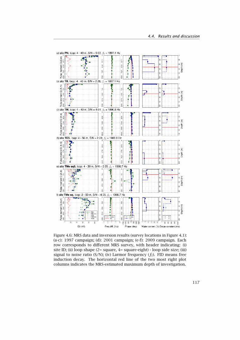
4.4. Results and discussion
Figure 4.6: MRS data and inversion results (survey locations in Figure 4.1):(a-c): 1997 campaign; (d): 2001 campaign; (e-f): 2009 campaign. Eachrow corresponds to different MRS survey, with header indicating: (i)site ID; (ii) loop shape (2= square, 4= square-eight) - loop side size; (iii)signal to noise ratio (S/N); (iv) Larmor frequency (fl). FID means freeinduction decay. The horizontal red line of the two most right plotcolumns indicates the MRS-estimated maximum depth of investigation.
117
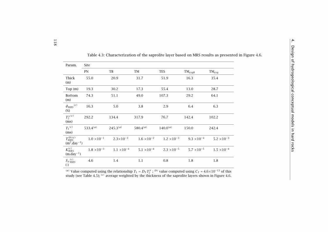
4.
Desig
nof
hyd
rogeo
logical
concep
tual
models
inhard
rock
s
Table 4.3: Characterization of the saprolite layer based on MRS results as presented in Figure 4.6.
Param. Site
PN TB TM TES TMesq8 TMesq
Thick(m)
55.0 20.9 31.7 51.9 16.3 35.4
Top (m) 19.3 30.2 17.3 55.4 13.0 28.7
Bottom(m)
74.3 51.1 49.0 107.3 29.2 64.1
θMRS(c)
(%)16.3 5.0 3.8 2.9 6.4 6.3
T∗2(c)
(ms)292.2 134.4 317.9 76.7 142.4 102.2
T1(c)
(ms)533.4(a) 245.3(a) 580.4(a) 140.0(a) 150.0 242.4
T (b)(c)MRS(m2.day−1)
1.0 ×10⁻¹ 2.3×10⁻³ 1.6 ×10⁻² 1.2 ×10⁻³ 9.3 ×10⁻⁴ 5.2 ×10⁻³
K(c)MRS(m.day−1)
1.8 ×10⁻³ 1.1 ×10⁻⁴ 5.1 ×10⁻⁴ 2.3 ×10⁻⁵ 5.7 ×10⁻⁵ 1.5 ×10⁻⁴
Sy(c)MRS(-)
4.6 1.4 1.1 0.8 1.8 1.8
(a) Value computed using the relationship T1 = DTT∗2 ; (b) value computed using CT = 4.6×10⁻¹³ of thisstudy (see Table 4.5); (c) average weighted by the thickness of the saprolite layers shown in Figure 4.6.
11
8

4.4. Results and discussion
At TMe, located within the F1 fault zone, we performed 2 interpretablesoundings using 2 overlapping MRS loops (Table 4.2): i) 30 m square-eight loop (Figure 4.6e); ii) 60 m square loop (Figure 4.6f). Remarkablewas that the surficial, alluvial layer detected by the 30 m square-eightloop was not detected by the 60 m square loop (Figure 4.6). This wasprobably because: (i) the saturated alluvial deposits are organized innarrow, shallow stream channels flanked by dry soil; (ii) the 30 m square-eight loop was placed right on top and along the alluvial channel; (iii) thenarrow, saturated alluvial layer was located on the periphery of the 60 msquare loop, so its contribution to the sensed signal was weak.
In several other sites along the fault zones, although saturated de-posits were observed with the groundwater observation network, weobtained weak or null MRS signal. This may be due to a low water con-tent and/or fine particle size, which produced respectively low MRS signaland short decay time constant that was close to or below instrumentdead-time (40 ms for NUMIS). At the other sites outside the fault zones(GJ, GB, MU), no valid MRS signal was obtained, which was explained bytoo low water content in fissured granite.
Hydrostratigraphy data integrationUsing hydrogeophysics, we could retrieve the following hydrostrati-graphic units in the Sardón area, from top to bottom: (i) a thin surficiallayer of alluvium with relatively high water content in the valleys; (ii) asaprolite layer; and (iii) a fissured layer (not detected with MRS). Alongthe F1 fault zone (TB, PN, TMe, TES), we identified the saprolite layer withthe 3 hydrogeophysical methods ERT, FDEM, MRS. MRS also indicated athin surficial layer of alluvium with relatively high water content above adeeper and thicker saprolite layer. A saprolite thickness larger than 45 mwas depicted along the F1 fault zone while along the F2 faults, it reached35 m. Along the pediment, the saprolite thickness was ∼20 m and locallyabsent at the planation of the hill tops. The width of the F1 fault zonewas ∼100 m although locally, as for example at PN location, it could beeven wider than 500 m. The width of the F2 fault zones was much lower,in order of 30 m. The fissured layer was only identified by ERT and FDEMmethods. It was located below the saprolite, at depth starting from 20to 40 m b.g.s. (sites TMe, TM, EM-TB). At the other sites (GJ, GB, MU),outside the F1 and F2 fault zones, the ERT showed the absence of thesaprolite layer (Figure 4.4). At these sites, we could not acquire any validMRS signal due to too low water content.
Table 4.4.4 presents the summary of the hydrostratigraphy resultsobtained by hydrogeophysical hard rock investigations in various worldlocations including our Sardón site. The saprolite and fissured layers inthe Sardón area are characterized by resistivity values of 10 to 100 Ω.mand 250 to 750 Ω.m respectively, while the fresh granite showed res-istivity above 1000 Ω.m. These values are in the same range as thoseobserved by other authors in other hard rock areas (Table 4.4). Alsothe MRS estimates (θMRS , T∗2 ) for saprolite are in the same range if we
119

4. Design of hydrogeological conceptual models in hard rocks
exclude the PN site that show unexpectedly high, saprolite θMRS = 16.3%.The hydrostratigraphy retrieved by hydrogeophysics was confirmed
by the drilling. A borehole at PN site intersected the saprolite down to24 m depth but we obtained a low borehole water yield that did notcorroborate the particularly high θMRS estimate. The borehole couldnot be made exactly at the same location as the MRS, which can explainthis difference. Other 2 drillings next to TMe (Figure 4.1) also confirmedthe presence of saprolite down to 38 m depth. Both of them also re-vealed very low water yield. At GJ, GB and MU, shallow boreholes andwells belonging to the local farmers allowed to observe directly the fis-sured zone at shallow depth (∼1-2 m b.g.s.). These observations arein agreement with what we observed at SD borehole site (Figure 4.1),where drilling intersected the fissured layer, starting at ∼2 to 3 m b.g.s.down to the borehole bottom at 48 m b.g.s. A disagreement betweenERT interpretation and borehole log was encountered at the TB site. Theborehole, located at ∼100 m north-east of the western part of the ERTcross-section TB (Figure 4.4, at ∼75 m horizontal scale), intersected thefissured zone, while ERT indicated the saprolite. This is likely due to thepresence of a F2 fault located between the ERT and the borehole (see TBsite on Figure 4.2) that brings in contact saprolite on the S block withfissured granite on the N block.
120

4.4
.R
esults
and
discu
ssion
Table 4.4: Hydrogeophysical results and comparison with other studies. ρ: electrical resistivity; θMRS : MRS free water content;T∗2 : free induction decay time constant.
Catchment. Saprolite Fissured granite
ρ (Ω.m) θMRS(%) T∗2 (ms) ρ (Ω.m) θMRS(%) T∗2 (ms)
Ringelbach(a) 50-800 <1.4 110-140 >800 <1.3 n.a.
(Brittany, France)
Margeride(a) 30-500 3-7 150-350 >500 n.a. n.a.
(Central Massif, France)
Kerbennez(a) 80-600 2.7-5.5 150-350 >600 <2 n.a.
(Brittany, France)
Andalatanousy(a) n.a. 2.2-5.5 50-180 n.a. <1 n.a.
(Madagascar)
Maheshwaram(a) 10-200 2-6 50-150 >200 <1 n.a.
(India) 30-120(b) 120-500(b)
Several in Brittany(a) n.a. 1.6-6.0 100-300 n.a. <2 n.a.
(France)
Burkina Faso(c) n.a. 1-6 180-600 n.a. 0.2-2.5 350-1500
(3) (400) (1.0) (650)
Moole Hole(d) 20-400 2.7 400-1000 1-2
(India)
Sardón(e) 10-100 2.9-16.3 75-320 250-750 <0.5 n.a.
(Salamanca, Spain) (6.8) (178)
n.a.: not available; when available, the average value is shown between parentheses. (a) Baltassatet al. (2005). (b) Dewandel et al. (2012). (c) Vouillamoz et al. (2005). (d) Legchenko et al. (2006);Descloitres et al. (2008); Chaudhuri et al. (2013). (e) This study.
12
1
4. Design of hydrogeological conceptual models in hard rocks
4.4.2 Aquifer parameters
Aquifer parameters were assessed by the MRS method, using Equations(4.2), (4.3) and (4.6) after MRS inversion and calibration against the slugtest transmissivities.
4.4.2.1 Flow parameters
In the MRS inversion results, we observed cases where basic nuclearmagnetic resonance (NMR) assumptions were not met so the T1 estimatoryielded a value that was lower than T∗2 . Such inversion results wererejected using the criteria of Equation (4.4). We assumed that part of theproblem was that the data inversion algorithm retrieved an overestimatedT∗2 when both water content and S/N were too low. Based on 5 validMRS measurements of the 2009 campaign, we obtained a saprolite DTvalue representative of the Sardón area of 1.83. Similar saprolite valueDT = 1.72 (mean of 6 values) was found in granites in Brittany (France)by Legchenko (2001). In contrast, Vouillamoz (2003) found significantlydifferent saprolite DT = 3.3 and DT = 6.5 in fissured granite with adataset composed of measurements in Brittany (France) and BurkinaFaso. However, he explained such high DT values by uncertainties inMRS measurement due to unfavorable S/N ratio and by heterogeneity ofthe magnetic field that influences T∗2 .
Out of the 5 boreholes with slug tests (Table 4.5 and Figure 4.1), 3were drilled in saprolite but only 2 were used for MRS calibration as 1 sitewas without MRS survey. We found very low saprolite slug test hydraulicconductivity (KST ) values, ranging from 5×10⁻⁴ to 2×10⁻³ m.d−1 andwith geometric mean of 7×10⁻⁴ m.d−1. We used the geometric meanbecause it is more representative than arithmetic mean or median whenthe dataset spreads over several orders of magnitude, which is thecase of hydrogeological parameters such as hydraulic conductivity. Thelow saprolite KST was consistent with field observations as the drillingcuttings showed fine particle size.
122
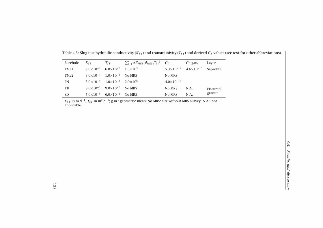
4.4
.R
esults
and
discu
ssion
Table 4.5: Slug test hydraulic conductivity (KST ) and transmissivity (TST ) and derived CT values (see text for other abbreviations).
Borehole KST TST∑ni=1∆ZMRSiθMRSiT1i
2 CT CT g.m. Layer
TMe1 2.0×10⁻³ 6.0×10⁻² 1.3×10⁵ 5.3×10⁻¹² 4.6×10⁻¹³ Saprolite
TMe2 3.0×10⁻⁴ 1.0×10⁻² No MRS No MRS
PN 5.0×10⁻⁴ 1.0×10⁻² 2.9×10⁶ 4.0×10⁻¹⁴
TB 8.0×10⁻³ 9.0×10⁻² No MRS No MRS N.A. FissuredgraniteSD 5.0×10⁻³ 6.0×10⁻² No MRS No MRS N.A.
KST in m.d−1, TST in m2.d−1; g.m.: geometric mean; No MRS: site without MRS survey. N.A.: notapplicable.
12
3
4. Design of hydrogeological conceptual models in hard rocks
The saprolite CT (Table 4.5) was computed according to Equation (4.5)at boreholes PN and TMe with saprolite layer down to 24 m and 40 m re-spectively. The saprolite layer was also depicted by the MRS (Figure 4.6a,e and f). The geometric mean of our two available CT estimates equals to4.6×10−13. That estimate is significantly lower than the CT = 8.2×10⁻¹⁰
estimate of the weathered granite of Burkina Faso (Vouillamoz et al.,2007). A possible reason could be in the method of hydrogeologicalsystem parameterization, as Vouillamoz et al. (2007) defined CT usingpumping test hydraulic conductivities (KPT ) while we used slug tests.Slug tests are prone to underestimation of K because they are represent-ative of a smaller volume around the borehole so the interconnectivityis not well represented, and therefore possibly underestimated. In con-trast, the volume of long-term pumping test is large enough to activateinterconnectivity over much larger volume than in slug test, resulting inlarger water release to the pump. The latter hypothesis can be debated asfor example in the granitic catchment of Maheswaram (India), Maréchalet al. (2004) found pretty low ratio of only 3:1 between average K frompumping tests and slug tests based on 6 boreholes with pumping testsand slug tests, although their hydrogeological conditions were quitedifferent than ours. Their geometric mean of saprolite KST of 30 slugtests was 0.4 m.d−1, i.e. 3 orders of magnitude larger than our KST =7×10⁻⁴ m.d−1. Another possible explanation of substantially lower val-ues of KST as compared to KPT was provided by Butler and Healey (1998)who attributed it to insufficient borehole-development prior slug test.That could be particularly relevant at typical low yield of the saprolite inour case. Finally, our substantially lower KST could be also because thehydrogeological conditions of our investigated sites were poorer thanthose of other authors mentioned above.
The saprolite MRS transmissivity (TMRS ) and hydraulic conductivity(KMRS ) defined using Equations (4.2) and (4.3) and CT = 4.6×10⁻¹³ arepresented in Table 4.3. The geometric mean of saprolite KMRS was1.6×10−4 m.d−1 with minimum and maximum values 2.3×10⁻⁵ and1.8×10−3 m.d−1 respectively. These values are very low as comparedto other studies possibly because of slug test related underestimationof CT as suggested earlier. Dewandel et al. (2006) presented a compila-tion of several studies in which the geometric mean of saprolite K was0.2 m.d−1 with minimum and maximum of 0.01 and 3.52 m.d−1 respect-ively. Legchenko et al. (2004) performed 11 MRS and 2 pumping teststo retrieve the transmissivity of a weathered-fissured granite aquifer inBrittany (France). They obtained an average saprolite KMRS similar orderof magnitude, i.e. 4.1 m.d−1 with minimum and maximum values were0.2 and 11.2 m.d−1 respectively. Although the KMRS that we found in theSardón area is much lower than the above quoted KMRS values, it is inagreement with the low yield observed in the boreholes. Besides, manywells drilled by the local farmers in the saprolite were abandoned due tolow yield and long recovery time.
The fissured layer was identified at sites GJ, FU, GB and MU with ERT.The MRS surveys targeting at fissured rocks at the FU and MU locations
124

4.4. Results and discussion
did not result in any valid MRS signal. The available information aboutpossible flow system parameterization originates from two borehole slugtests (Table 4.5). The KST of the fissured granite layer in TB and SD slugtest sites were 8×10⁻³ m.d−1 and 5×10⁻³ m.d−1 respectively (Table 4.5),corresponding to a geometric mean of 6×10⁻³ m.d−1, so one order ofmagnitude higher than the KST of the saprolite layer.
It is not only in this study but overall that there is scarcity of success-ful MRS measurements in fissured rocks (Table 4.4). The only publisheddata we found (Table 4.4) originates from Burkina Faso study (Vouillamozet al., 2005). Based on a dataset composed of 13 MRS measurements,they presented an average, fissured rock T1 = 650 ms (average θMRS = 1%)that was larger than saprolite T1 = 400 ms (average θMRS = 3%), indicatinga higher transmissivity in the fissured layer than in the saprolite andthus confirming the hard rock general conceptual model.
4.4.2.2 Storage parameters
As the saprolite aquifer at the Sardón catchment was unconfined, wecomputed SyMRS using Equation (4.6) with a Cy value of 2.8×10⁻¹ as-signed in weathered granite in Burkina Faso (Vouillamoz et al., 2007). Theaverage SyMRS was 1.9% with minimum of 0.8% and maximum of 4.6%.However, it is expected that our Sy may be lower due to the fine particlesize of the saprolite in the Sardón area. To our knowledge the saproliteCy value for weathered granite found in Vouillamoz et al. (2005) andVouillamoz et al. (2007) are the only available hard rock Cy estimates inthe scientific literature.
In the fissured layer, as it was not possible to acquire MRS signal,it was assumed that its water content was <0.5%, i.e. the consideredMRS detectability threshold (Legchenko et al., 2006). Fissured rockestimates of Cy and Ce are not available yet in the literature. This islikely because computing Cy and/or Ce multipliers, requires cumbersomeand expensive estimation of Sy and/or Se by piezometric pumping tests.
4.4.2.3 Perspectives of aquifer parameterisation
Although we had some difficulties in acquiring MRS data of the saprolitelayer, the most challenging was to acquire valid MRS signal of the fis-sured layer. The fissured layer constitutes a low storage but significanthydraulic conductivity target. In this regard, the first item to consider isthe optimization of the loop size, shape and for some shapes, orientationto the particular targets i.e. sometimes layers parallel to ground butother times to structural features such as sub-vertical linear features orintersection of such features. Moreover, given the low water content ofthe fissure zone, various strategies to improve S/N must be consideredto optimize signal level while noise attenuation/compensation strategiesmust be improved. Large bandwidth instrumentation allows detectingwater in thin fractures, in the unsaturated zone and also in the moreclayey sands than what was possible with the "classical" MRS. The in-
125
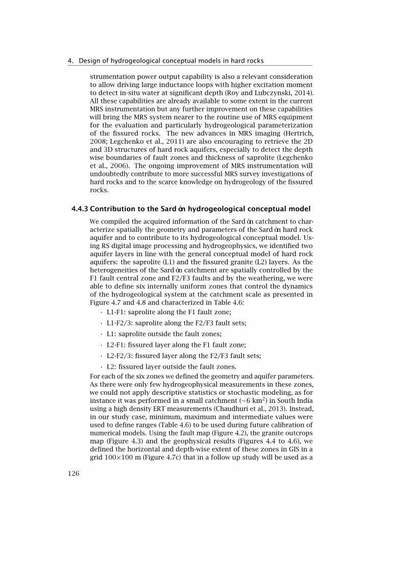
4. Design of hydrogeological conceptual models in hard rocks
strumentation power output capability is also a relevant considerationto allow driving large inductance loops with higher excitation momentto detect in-situ water at significant depth (Roy and Lubczynski, 2014).All these capabilities are already available to some extent in the currentMRS instrumentation but any further improvement on these capabilitieswill bring the MRS system nearer to the routine use of MRS equipmentfor the evaluation and particularly hydrogeological parameterizationof the fissured rocks. The new advances in MRS imaging (Hertrich,2008; Legchenko et al., 2011) are also encouraging to retrieve the 2Dand 3D structures of hard rock aquifers, especially to detect the depthwise boundaries of fault zones and thickness of saprolite (Legchenkoet al., 2006). The ongoing improvement of MRS instrumentation willundoubtedly contribute to more successful MRS survey investigations ofhard rocks and to the scarce knowledge on hydrogeology of the fissuredrocks.
4.4.3 Contribution to the Sardón hydrogeological conceptual model
We compiled the acquired information of the Sardón catchment to char-acterize spatially the geometry and parameters of the Sardón hard rockaquifer and to contribute to its hydrogeological conceptual model. Us-ing RS digital image processing and hydrogeophysics, we identified twoaquifer layers in line with the general conceptual model of hard rockaquifers: the saprolite (L1) and the fissured granite (L2) layers. As theheterogeneities of the Sardón catchment are spatially controlled by theF1 fault central zone and F2/F3 faults and by the weathering, we wereable to define six internally uniform zones that control the dynamicsof the hydrogeological system at the catchment scale as presented inFigure 4.7 and 4.8 and characterized in Table 4.6:
• L1-F1: saprolite along the F1 fault zone;
• L1-F2/3: saprolite along the F2/F3 fault sets;
• L1: saprolite outside the fault zones;
• L2-F1: fissured layer along the F1 fault zone;
• L2-F2/3: fissured layer along the F2/F3 fault sets;
• L2: fissured layer outside the fault zones.
For each of the six zones we defined the geometry and aquifer parameters.As there were only few hydrogeophysical measurements in these zones,we could not apply descriptive statistics or stochastic modeling, as forinstance it was performed in a small catchment (∼6 km2) in South Indiausing a high density ERT measurements (Chaudhuri et al., 2013). Instead,in our study case, minimum, maximum and intermediate values wereused to define ranges (Table 4.6) to be used during future calibration ofnumerical models. Using the fault map (Figure 4.2), the granite outcropsmap (Figure 4.3) and the geophysical results (Figures 4.4 to 4.6), wedefined the horizontal and depth-wise extent of these zones in GIS in agrid 100×100 m (Figure 4.7c) that in a follow up study will be used as a
126

4.4. Results and discussion
reference for distributed numerical groundwater model. The width of thefault zones, as retrieved by ERT and FDEM, was between 30 m and 600 m.As the fracture spacing observed in the field was between few centimetersto several meters (Attanayake, 1999), the 100 m grid resolution insuredthat the connectivity between fractures was taken into account. L1 is onlypresent where L2 is not outcropping (Figure 4.7a) while L2 is assumedto extend over the entire catchment (Figure 4.7b). The saprolite layer L1is hydrogeologically defined as an unconfined layer while the fissuredlayer L2 as confined layer when not outcropping. We assumed that L2is underlain by non-fractured bedrock that constitutes the imperviousbottom boundary. The fault zones fully control the hydrogeology of thecatchment and connect hydraulically L1 and L2 layers. This fact wasconfirmed by borehole drillings that showed consistent, similar waterlevels in both fissured and saprolite layers. Groundwater is drainedalong the F2/F3 fault zones towards the main F1 fault zone and thenalong that F1 fault zone towards the catchment outlet at the north of thecatchment.
127

4.
Desig
nof
hyd
rogeo
logical
concep
tual
models
inhard
rock
s
Figure 4.7: Hydrogeological conceptual model maps: a) active cells of layer L1 (saprolite), indicated in light brown; b) activecells of layer L2 (fissured layer), indicated in pink; c) fault zones within the L1 and L2 layers (see corresponding parameters inTable 4.6).
12
8

4.4
.R
esults
and
discu
ssion
Figure 4.8: Schematic cross-section transversal to the main catchment valley of the hydrogeological conceptual model of theSardón catchment (see corresponding parameters in Table 4.6).1
29

4.
Desig
nof
hyd
rogeo
logical
concep
tual
models
inhard
rock
s
Table 4.6: Parameters of the hydrogeological conceptual model (see distribution of zones in Figures 4.7 and 4.8).
Zone Thickness (m) K (m.d−1) T (m2.d−1)
int. min. max. int. min. max. int. min. max.
L1-F1 45.0 20.0 75.0 7.4×10⁻³ 4.6×10⁻⁴ 1.4×10⁻¹
L1-F2/3 35.0 5.0 50.0 1.6×10⁻⁴ 2.3×10⁻⁵ 1.8×10⁻³ 5.8×10⁻³ 1.2×10⁻⁴ 9.0×10⁻²
L1-nF(a) 20.0 1.0 40.0 3.3×10⁻³ 2.3×10⁻⁵ 7.2×10⁻²
L2-F1 67.5 30.0 112.5 1.1×10⁻¹ 6.9×10⁻³ 2.0
L2-F2/3 52.5 7.5 75.0 1.6×10⁻³(b) 2.3×10⁻⁴(b) 1.8×10⁻²(b) 8.6×10⁻² 1.7×10⁻³ 1.4
L2-nF 30.0 1.0 60.0 4.9×10⁻² 3.5×10⁻⁴ 1.1
int.,min.,max: intermediate,minimum and maximum values respectively; N.A.: not applicable; (a): where L2outcrops, the thickness of the L1 layer is null; b): corresponds to the K value of the L1 layer multiplied by 10. K,T , Sy and Se are respectively hydraulic conductivity, transmissivity, specific yield and elastic storativity.
Continued on next page
13
0

4.4
.R
esults
and
discu
ssion
– continued from previous page
Zone Sy (-) Se (-)
int. min. max. int. min. max.
L1-F1
L1-F2/3 1.90 0.80 4.60 N.A. N.A. N.A.
L1-nF(a)
L2-F1 1.0×10⁻³ 4.0×10⁻⁴ 3.0×10⁻³
L2-F2/3 0.50 0.05 1.00 1.0×10⁻³ 4.0×10⁻⁴ 3.0×10⁻³
L2-nF 4.0×10⁻³ 2.0×10⁻⁴ 7.0×10⁻³
13
1
4. Design of hydrogeological conceptual models in hard rocks
In the most elevated parts of the catchment, the outcrop mapping (Fig-ure 4.3) and ERT interpretation of the FU, GJ, GB and MU sites (Figure 4.4)showed that the saprolite layer is absent. The absence of saprolite isprobably due to tectonic uplift that provoked erosion, while the saprolitewas preserved in depressions (López, 2004). The mapping of the erosionsurfaces (Instituto Geológico y Minero de España, 1991a,b) supports thishypothesis. The elevation of the top of the L1 saprolite layer was ob-tained by subtracting the soil thickness (eluvium and alluvium) retrievedby GPR and direct observations (drilling with portable gasoline poweredpercussion hammer) from the ground surface of the digital terrain model(Figure 4.2a) resampled at 100 m resolution. The thickness of the L1saprolite layer (Table 4.6) was defined based on the interpretation ofERT, FDEM and MRS. The assessment of the thickness of the L2 fissuredlayer is a complex and uncertain matter. Lachassagne et al. (2011) madea review of studies in hard rock aquifers and stated that the "thicknessof the fissured layer is approximately two to three times that of thesaprolite". Dewandel et al. (2006) presented a ratio of 2 in the descrip-tion of the hard rock aquifer general conceptual model, considering asingle weathering event. In the Maheshwaram catchment (India), thesame authors found a ratio of 1 that they explained by the erosion of thesaprolite layer before the development of a new, actual weathering front.In Sardón catchment, we assumed that the L2 fissured layer was 1.5 timesthicker than the L1 saprolite layer. It is coherent with the geologicalhistory of the area, which was affected during the Alpine orogeny byseveral uplifting events and related erosion of the saprolite (López, 2004).With ratio 1.5 we obtained L2 transmissivity of one order of magnitudehigher than the transmissivity of L1 (Table 4.6).
The ranges of aquifer parameters were defined using the results of thehydrogeophysical analysis elaborated in the previous section. Althoughthe flow parameters (KMRS and TMRS ) computed with the CT value definedfor the Sardón site are generally low, they well reflect field observations.As it was not possible in this study to retrieve the parameters of thefissured zone, we used the results and concepts presented in previousstudies of Dewandel et al. (2006), Dewandel et al. (2011) and Lachassagneet al. (2011). The model of a hard rock aquifer that these authorsdefined states that the fissured layer has higher transmissivity thanthe saprolite layer. They observed that K in the fissured layer was ∼1order of magnitude higher than K in the saprolite layer (Figure 13 inDewandel et al. (2006); Figure 8 in Dewandel et al. (2011); Figure 7 inLachassagne et al. (2011)). As we observed similar relation with slugtests, we estimated the K values of the fissured layer as one order ofmagnitude higher than our saprolite K values (Table 4.6).
Although we had to make some assumptions to parameterize the L1and L2 reservoirs, the presented hydrogeological conceptual model isbased on field observations and measurements hydrogeophysically andhydrogeologically sound. Similar approach was applied by Boucher et al.(2009a); Chaudhuri et al. (2013); Baroncini-Turricchia et al. (2014). Suchmethodology allows to avoid in groundwater model design the arbitrary
132

4.5. Conclusion
and artificial definition of uniform, parametric zones around observationpoints that ensure a good fit between simulated and observed state vari-ables (soil moisture, hydraulic heads) (Voss, 2011). Indeed, a calibratedmodel that reproduces accurately the measured state variables is notnecessarily a good model, particularly in complex hard rock conditions,in the sense that it will probably fail in validation and prediction. In thisstudy, we limited the number of aquifer parameter zones from what wasobserved by the downward approach. We designed a hydrogeologicalconceptual model, defining a range of aquifer parameters and aquiferthicknesses that will allow us to constrain the numerical groundwatermodel and to reduce the number of equivalent solutions during the cal-ibration process. Nevertheless, there is still a need of a better hard rocksystem’s parameterization, particularly the parameterization of fissuredzone. This, instead of expensive boreholes and pumping tests, can prob-ably be achieved by MRS but only after some substantial improvementstargeting at fissured rock assessment.
4.5 Conclusion
We proposed a multi-technique methodology to contribute to the designof hydrogeological conceptual model in hard rock aquifers. The methodis based on a downward approach that combines: (i) remote sensingtechniques such as digital image processing on satellite images anddigital terrain models; (ii) hydrogeophysics; and (iii) hydrogeologicalfield data acquisition. We applied that method to the hard rock Sardóncatchment, contributing to the improvement of the hydrogeological con-ceptual model of that area. In particular we identified the saprolite andfissured layers and characterized their geometry (i.e. horizontal extentand thickness) as well as the spatial variation of the aquifer parameters(flow and storage properties). We drilled 5 boreholes to validate andcalibrate the hydrogeophysical data, showing that the methodology is ap-plicable in data scarce areas. The processing of high-resolution satelliteimages and digital terrain model allowed mapping efficiently the mainfault zones and the horizontal distribution of the hydrostratigraphiclayers. The GPR method was able to detect shallow water table althoughthe quantitative assessment of the water table depth could not be maderoutinely because it required local calibration based on measurementsmade in piezometers and soils and was restricted to the locations withwater table depth <3 m b.g.s. The ERT method allowed to confirm localsubsurface hydrostratigraphy and provided input for the MRS inver-sion. The multi-frequency FDEM method combined with the laterallyconstrained inversion technique showed to be very efficient, providinglong cross-sections depicting large hydrogeological structures coherentwith direct field observation, geological mapping and drilling. The MRSprovided valuable results in the saprolite layer, but only in the locationswith sufficient signal to noise ratio. Unfortunately, more than half of theMRS survey locations had too low water content to be sensed with the
133

4. Design of hydrogeological conceptual models in hard rocks
MRS equipment we used. The optimization of MRS loops to this type oftargets and the use of improved instrumentation (larger pulse moment,better noise rejection capability and shorter dead-time) is recommendedto improve MRS data acquisition in the Sardón catchment and in all hardrock aquifers characterized by low or very low water content.
The method of hydrogeological characterization of complex hardrock catchments presented in this study is time and cost effective, buthighly suitable for development of hydrogeological conceptual modelsin fractured hard rocks which otherwise require large time and costinvestments. The iterative process of hydrogeological conceptual modeldevelopment constitutes a powerful tool to synthetize the knowledgeof various sources and to define optimal strategy of complementarydata acquisition, providing reliable basis for development of numericaldistributed models.
134
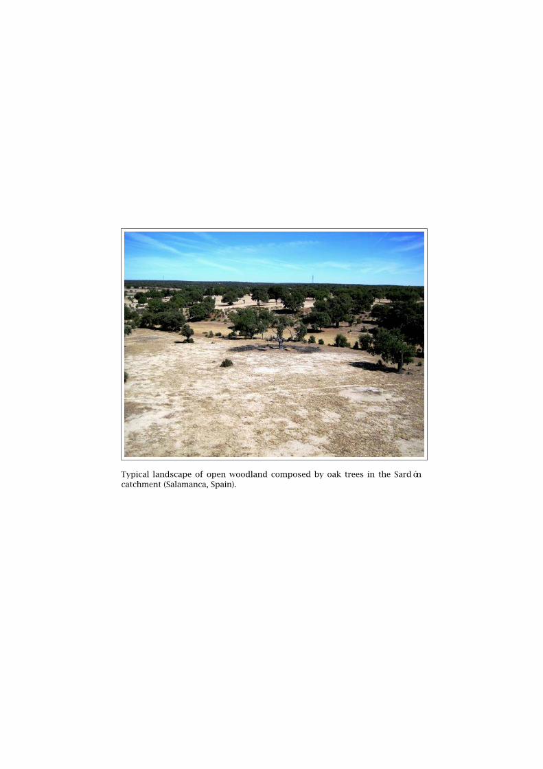
Typical landscape of open woodland composed by oak trees in the Sardóncatchment (Salamanca, Spain).

5Partitioning and sourcing ofevapotranspiration at thecatchment scale using coupledMARMITES-MODFLOW model
5.1 Introduction
Numerical groundwater flow models constitute a powerful tool forgroundwater management as they allow to predict aquifers dynamicresponses in relation to climatic, land use and abstraction changes.Groundwater models require both an accurate physical representation ofan aquifer system and appropriate boundary conditions. While aquiferparameters as hydraulic conductivity (K) and storativity (S) are spatiallydependent and time invariant, groundwater fluxes such as gross recharge(Rg), groundwater evapotranspiration (ETg), groundwater exfiltration(Exfg) and groundwater inflow/outflow (respectively Qi and Qo) canvary in both space and time. Multiplicity of combinations between para-meters and fluxes leads to non-uniqueness of model solutions, whichlimits their reliability and forecasting capability (Moore and Doherty,2006; Batelaan and de Smedt, 2007).
One possible approach to minimize non-uniqueness of model solu-tions is to invest in a better spatial parametrization of the subsur-face reservoirs, for instance by applying hydrogeophysical techniques(Francés and Lubczynski, 2011; Baroncini-Turricchia et al., 2014; Francéset al., 2014, 2015). Another approach is to constrain groundwater modelswith spatio-temporally variable groundwater fluxes (Jyrkama et al., 2002;Lubczynski and Gurwin, 2005), although such assessment is complex(Kinzelbach et al., 2002; Hendricks et al., 2003; Xu and Beekman, 2003;Lubczynski and Gurwin, 2005; Lubczynski, 2011), because: (i) subsur-
This chapter is based on: Partitioning and sourcing of evapotranspiration at thecatchment scale using coupled MARMITES-MODFLOW model. Francés, A. P., and M. W.Lubczynski (2015), submitted to Water Resource Research
137

5. Coupled MARMITES-MODFLOW model
face water fluxes, due to their inaccessibility, are by far more difficult toquantify than surface water fluxes and consequently the methods of theirestimation are highly uncertain; (ii) subsurface water fluxes are controlledby spatio-temporal variability of rainfall (RF ) and evapotranspiration(ET ) but also by surface and subsurface heterogeneity of geology, soiltexture, topography, drainage, vegetation, etc.; (iii) groundwater fluxesare generally small and Rg cannot be reliably determined (particularlyin water limited areas where Rg is low) by subtracting ET from RF ,since unavoidable small errors in the two lead to high inaccuracy of Rg(Lubczynski, 2011); (iv) ETg is generally underestimated (Lubczynski,2000, 2009), which results in the overestimation of the net recharge(Rn = Rg − Exfg − ETg) and therefore erroneous model calibration; and(v) standard groundwater models do not take into account interactionswith unsaturated zone so also do not quantify Exfg that can representimportant component of groundwater balance (Hassan et al., 2014).
For many years it has been a common modeling practice, while usingstandalone groundwater models, to apply arbitrary, simplistic estim-ates of groundwater fluxes (typically ETg and Rg) that were adjusteda-posteriori during model calibration. However, such practices haveoften been leading to large biases in parameter estimation and erroneousgroundwater balances (Batelaan and de Smedt, 2007; Lubczynski, 2009,2011; Hassan et al., 2014). The relevance of integrating subsurface fluxes,i.e. not only groundwater but also unsaturated zone fluxes, in hydrolo-gical modeling and water balancing has recently been emphasized andimportant advances have been made (Niswonger et al., 2006; Markstromet al., 2008; Twarakavi et al., 2008; Lubczynski, 2011; Hassan et al., 2014).Distributed and transient water balance models that simulate surface,unsaturated zone and saturated zones processes, so called coupled mod-els, constitute an efficient way to compute spatio-temporally a catchmentwater balance through partitioning of rainfall into evapotranspiration,runoff, storage and groundwater recharge.
An important component of the coupled models are unsaturatedzone models, as they link surface and groundwater domains. The mostadvanced are physically based unsaturated zone models that involve theDarcy’s law and the law of mass conservation expressed through theRichards’ equation. Examples of such models are SWAP (Kroes and vanDam, 2003), VSF (Thoms et al., 2006) and HYDRUS (Šimunek et al., 2011).However, the Richards’ equation is highly non-linear and its numericalsolution is computationally demanding. It requires a complex paramet-rization and boundary condition definition, which rather restricts itsapplication to local scale models (Niswonger et al., 2006; Thoms et al.,2006; Sheikh et al., 2009). At the catchment scale, simplified repres-entations of the physical processes are generally applied because theylimit the number of parameters to commonly available field informa-tion (Yates, 1996; Rushton et al., 2006; Sheikh et al., 2009). Typicalsimplifications applied in unsaturated zone models are based on thekinematic wave approximation of the Richards’ equation (Singh, 1997;Beven and Freer, 2001) and on lumped-parameterization as in WATBAL
138

5.1. Introduction
(Yates, 1996), SLURP (Kite, 2000), DREAM (Manfreda et al., 2005), BEACH(Sheikh et al., 2009), INFIL (U.S. Geological Survey, 2008) and others(Finch, 2001; Rushton et al., 2006). Despite the simplification, kinematicwave approximation and lumped parameter models proved to performat the catchment scale as good as the physically based models (Gehrels,2000; Sheikh et al., 2009). For instance, Soylu et al. (2011) tested theimpact of groundwater depth on ET in a semi-arid grassland region andconfirmed that when using standard soil hydraulic parameter datasets,the HYDRUS-1D model (Šimunek et al., 2008) and a single-bucket soilmoisture model performed equivalently well at the large, regional scale.This is because the simplification due to grid-cell averaging of the soilhydraulic parameters makes the two solutions comparable. These au-thors also showed that both models performed much better when thegroundwater depth was introduced as bottom boundary condition.
Relatively simple coupling is when an unsaturated zone model iscoupled with an analytical groundwater model. One of such models isVisual Balan (Samper et al., 2005), in which soil water balance is coupledwith a simple drainage analytical model that represents an aquifer system.As a lumped model, Visual Balan provides a single flux value of the entirecatchment and is thus limited to small, homogeneous areas. Similar solu-tion is the process-based, catchment-scale SWAT model, widely appliedin water use and water quality studies (Gassman et al., 2007; Douglas-Mankin et al., 2010). That semi-distributed model divides a catchmentinto multiple sub-catchments, which are then further subdivided intohydrologic response units that consist of lumped areas with homogen-eous land use, management and soil characteristics. The groundwaterreservoir is simplified into two aquifers, one shallow and unconfined andanother deep and confined, both modeled using analytical equations.
More sophisticated coupling is when unsaturated zone model iscoupled with physically based, distributed numerical model that appliesgroundwater flow and storage equation (Fetter, 2001), as for instancestandalone MODFLOW (Harbaugh et al., 2000). Stanton et al. (2013)showed that the performance of MODFLOW could be improved by itslinking to a lumped parameter soil water balance model that providedthe spatio-temporal distribution of recharge. Similarly, Batelaan andde Smedt (2007) coupled a distributed water balance model (WetSpass)with steady-state MODFLOW. That modeling approach allowed to integ-rate the inter-influence between recharge and groundwater depth andto depict high spatial variation of Rn, with negative values in valleysdue to shallow groundwater table and substantial ETg of phreatophyticvegetation. Dams et al. (2012) went further by introducing the temporalvariability in the coupling of WetSpa (Wang et al., 1996), a process-based,lumped parameter, transient and distributed hydrological model, withMODFLOW. WetSpa can simulate at daily time step river discharge andpercolation out of the root zone, which are further assimilated into MOD-FLOW groundwater recharge at half-month time-step. In that solutionhowever, the delay between percolation from root zone and groundwaterrecharge due to water transport through the unsaturated zone was not
139

5. Coupled MARMITES-MODFLOW model
considered. Moreover, the one-way coupling, i.e. exchange of bound-ary conditions from one model to another, did not allow to include thegroundwater table depth effect on the soil reservoir. That problem iswell handled for example by Sophocleous and Perkins (2000), Kim et al.(2008) and Chung et al. (2010) who replaced the groundwater analyticalmodule of the quasi-distributed catchment SWAT model with the fully-distributed groundwater MODFLOW model. They applied a two-way coup-ling between SWAT and MODFLOW, i.e. the two models could exchangebetween them boundary conditions, which enabled interaction betweensaturated zone and channel reaches, as well as the simulation of spatio-temporal distribution of groundwater recharge rates, aquifer evapotran-spiration and groundwater levels. Another two-way coupled model isthe public domain, distributed hydrological model GSFLOW (Markstromet al., 2008). GSFLOW fully couples PRMS, a lumped-parameter, physical-process catchment precipitation-runoff model (Leavesley et al., 1983),with MODFLOW-NWT (Niswonger et al., 2011). In that coupling, the MOD-FLOW package UZF1 (Niswonger et al., 2006) simulates unsaturated zoneflow using a 1D vertical kinematic wave approximation of the Richards’equation. Another similar solution is a distributed version of the one-dimensional unsaturated flow package HYDRUS coupled with MODFLOW(Seo et al., 2007; Twarakavi et al., 2008). The HYDRUS package providesMODFLOW with recharge fluxes, while MODFLOW provides HYDRUS withthe elevation of the groundwater table that is used as the bottom bound-ary condition in the package. The integrated catchment MIKE SHE modelalso integrates groundwater and surface water, taking into account thepartitioning of rainfall into runoff, evapotranspiration and groundwaterrecharge. One important advantage of MIKE SHE is that it allows theuser to select the degree of complexity of the application. For instance,vertical unsaturated flow may be modeled either by 1D, finite differencemultilayer method based on Richards’ equation or by a simpler, two-layerroot zone model. This allows to apply MIKE SHE either as fully physicalmodel at the local scale or using simplified physical equations to run themodel at the regional scale. However, MIKE SHE is not public domain andparametrically demanding.
The most advanced and complex models are fully integrated hydro-logic models such as InHM (van der Kwaak, 1999; van der Kwaak andLoague, 2001), HydroGeoSphere (Brunner and Simmons, 2012; Therrienet al., 2012) and ParFlow (Kollet and Maxwell, 2006, 2008) (for a reviewand comparison of integrated hydrologic models refer to Maxwell et al.(2014)). These models simulate land surface, unsaturated and saturatedzone flow processes based on adapted forms of the Richards’ and SaintVenant (overland flow) equations that are mathematically integratedand solved simultaneously. The main restriction to their use, besidesthe extensive parameterization, is that they are highly demanding incomputing resources and require high-performance parallel computers.
The most advanced models of the presented review allow to com-pute a detailed spatio-temporal water balance at the catchment scaleand implement the separation, here referred as sourcing, of ET into
140

5.2. Material and Methods
unsaturated zone and groundwater evapotranspiration (respectively ETuand ETg). Indeed, it is already well known and scientifically acceptedthat ET affects not only the surface and unsaturated zones but also thesaturated zone, representing important components of water balances(Miller et al., 2010; Lubczynski, 2011; Balugani et al., 2015). However,as the evapotranspiration represents two physically different processes,evaporation (E) and transpiration (T ), with two different spatial andtemporal characteristics (Guan and Wilson, 2009; Lubczynski, 2011; Orel-lana et al., 2012), hydrological models need to account them separately.Therefore, not only the sourcing but also the partitioning of ET into Tand E have to be implemented into hydrological models, by consideringthe following subsurface ET components: unsaturated zone evapora-tion (Eu), groundwater evaporation (Eg), unsaturated zone transpiration(Tu) and groundwater transpiration (Tg). The partitioning and sourcingof evapotranspiration fluxes is relevant not only to improve reliabilityof models and their water balances but also to understand the role ofvegetation and soil processes in the water cycle and to make reliableprediction scenarios of climate and land use changes (Lubczynski, 2011).
This chapter introduces a transient and distributed lumped-parametermodel of the land surface and the soil zone MARMITES that is two-waycoupled with the groundwater model MODFLOW-NWT (Niswonger et al.,2011). This coupled model computes spatio-temporally a detailed waterbalance at the catchment scale. The main novelties of the proposedapproach are: (i) partitioning of the evapotranspiration into evaporationand transpiration; (ii) sourcing of evaporation and transpiration intounsaturated and saturated zone components; and (iii) integration of (i)and (ii) in the newly developed MARMITES-MODFLOW coupled model.The objective of this study is to present the capacity of the MARMITES-MODFLOW model to quantify spatio-temporally surface and subsurfacewater fluxes with emphasis on partitioning and sourcing of subsurfaceevapotranspiration. This presentation is done on the base of the small(∼4.8 km2) La Mata Catchment case study (Salamanca, Spain).
5.2 Material and Methods
5.2.1 MARMITES-MODFLOW Coupled Model
5.2.1.1 General MARMITES-MODFLOW Description
MARMITES (MM) is a transient, distributed model of the land surface andthe soil zone that is coupled with the groundwater model MODFLOW(MF). Both models share the same spatial and temporal discretization.Figure 5.1 (right) shows the structure of one cell of the two models of theMM-MF coupling. MM is composed of one surface component (MMsurf)and one soil zone component (MMsoil). The unsaturated zone below thebottom of the soil zone and above the groundwater table, referred hereas percolation zone, is modeled using UZF1 package (Niswonger et al.,2006), while the groundwater flow in the saturated zone is handled by
141

5. Coupled MARMITES-MODFLOW model
MODFLOW-NWT (Niswonger et al., 2011). The following processes areconsidered in MM-MF: (i) rainfall interception by vegetation and crops(MMsurf); (ii) irrigation in agricultural fields (MMsurf); (iii) computing ofpotential evaporation and potential transpiration of several vegetation,crop and soil types (MMsurf); (iv) runoff, surface storage and evaporationfrom open water (MMsurf); (v) infiltration, evaporation, transpiration,percolation and soil moisture storage of the soil zone (MMsoil); (vi) per-colation and storage in the percolation zone (MF-UZF1); (vii) groundwaterrecharge, evaporation, transpiration, flow and storage in the saturatedzone (MF). A detailed description of the MM components and MF pack-ages, including input data, parameters and equations, is available insection 5.2.1.2.
The abbreviations keys of Figure 5.1 are as following:
• Land surface: rainfall RF , rainfall excess RFe, interception I, sur-face water evaporation Esurf , surface runoff Ro, storage Ssurf .
• Soil zone: infiltration Inf , soil evaporation Esoil, soil transpirationTsoil, percolation Rsoil, saturated soil exfiltration Exf , storage Ssoil,l is the number of soil layers.
• Percolation zone: percolation zone evaporation Ep, percolationzone transpiration Tp, percolation from the soil zone Rp, grossrecharge Rg, storage Sp.
• Saturated zone: groundwater evaporation Eg , groundwater tran-spiration Tg , groundwater exfiltration Exfg , inflow/outflowQi/Qo,storage Sg , L is the number of aquifer layers.
142
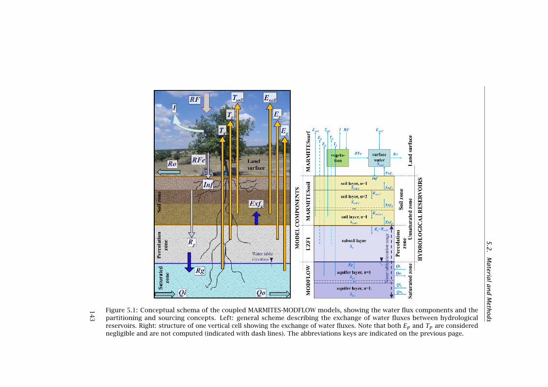
5.2
.M
ateria
land
Meth
ods
Figure 5.1: Conceptual schema of the coupled MARMITES-MODFLOW models, showing the water flux components and thepartitioning and sourcing concepts. Left: general scheme describing the exchange of water fluxes between hydrologicalreservoirs. Right: structure of one vertical cell showing the exchange of water fluxes. Note that both Ep and Tp are considerednegligible and are not computed (indicated with dash lines). The abbreviations keys are indicated on the previous page.
14
3

5. Coupled MARMITES-MODFLOW model
A typical MM-MF run is initiated by the MMsurf component (Figure 5.1and section 5.2.1.2). The main function of MMsurf is to compute ondaily basis the driving forces (rainfall, potential evaporation and poten-tial transpiration). Subsequently, the rainfall partitioning and relatedwater balance in the soil zone is computed on daily basis by the MMsoilcomponent using lumped-parameters and linear relationships betweenfluxes, driving forces and soil moisture (Figure 5.1 and section 5.2.1.2).The soil zone is typically discretized into superimposed layers that areparameterized with basic soil hydraulic properties. Generally these soillayers are defined using textural criterion and correspond to the A and Bhorizons, which are the zones of eluviation and illuviation respectively(Dingman, 2002; Food and Agriculture Organization, 2006). The user canalternatively define one single soil zone corresponding to the root zone.The percolation output from the soil zone is introduced as input of theMF UZF1 package (Niswonger et al., 2006). UZF1 in the MM-MF couplingframework simulates the water flow through the percolation zone, i.e.the zone below the soil bottom and above the groundwater table. Thiszone corresponds to the C and R horizons, i.e. parent material andbedrock respectively. UZF1 considers only one single uniform layer andconverts percolation from MMsoil into groundwater recharge by applyinga 1D kinematic-wave approximation of the Richards’ equation that onlyincorporates gravitational forces and neglects capillary ones (Niswongeret al., 2006). If the groundwater table rises above the bottom of the MMsoil layer, groundwater exfiltration (Exfg) from the aquifer into the MMsoil zone occurs, hypothetically creating runoff if the soil layers turnsaturated. If that happens, the MF hydraulic heads are corrected in MMto add the thickness of the saturated soil layers. Finally, water flowand storage in the saturated zone are computed by MF (section 5.2.1.2).The MM-MF coupled model output is a daily, grid-based water balanceof the catchment that can be visualized by maps, time series plots andanimations (spatio-temporal variability of fluxes). The yearly averagedwater balance at the observation plots and at the catchment scale can beplotted as Sankey diagrams. Such representation eases the visualizationof the water balance because: (i) the simulated fluxes are represented byarrows with width proportional to the water flux they represent; and (ii)these arrows are connected, representing the exchange of water betweenthe model reservoirs.
5.2.1.2 MM-MF Detailed Description
The water balance at the catchment scale in the MM-MF modeling frame-work is computed considering storage, flux and exchange of waterbetween the following 4 main reservoirs (Figure 5.1): land surface, soilzone, percolation zone and saturated zone. In the text below, the in-dex surf refers to the surface, index soil to the soil zone, index p to thepercolation zone and the index g to the saturated zone. The full list ofinput parametric maps is presented in Table 5.1.
144

5.2. Material and Methods
Table 5.1: MM-MF input parametric maps. Each map can be defined asan ASCII ESRI raster file or a unique scalar value. For MF, an input isrequired for each layer.
Name Description Unit
gridMETEO_fn meteorological zones [-]
gridIRR_fn irrigated field [-]
gridSOIL_fn soil type [-]
gridSOILthick_fn thickness of the soil m
gridPONDhmax maximum water height in the cell stream m
gridPONDw width of the cell stream m
elev topography m
thick thickness of the MF layers m
ibound MF active cells [-]
strt MF initial hydraulic heads m
hk MF horizontal hydraulic conductivity m.s−1
vka MF vertical hydraulic conductivity m.s−1 or [-]
Sy MF specific yield m3.m−3
Ss MF specific storage [-]
iuzfbnd MF UZF1 active recharge/discharge cells [-]
vks MF UZF1 saturated vertical hydraulic conductiv-ity of the unsaturated zone
m.s−1
eps MF UZF1 Brooks-Corey epsilon of the unsatur-ated zone
[-]
thts MF UZF1 saturated water content of the unsatur-ated zone
m3.m−3
thti MF UZF1 initial water content of the unsaturatedzone
m3.m−3
gbh_head MF GHB hydraulic head m
gbh_cond MF GHB hydraulic conductance m2.m−3
drn_elev MF DRN drain elevation m
drn_cond MF DRN hydraulic conductance m2.m−3
145
5. Coupled MARMITES-MODFLOW model
MARMITES SurfaceThe surface water balance equation is written as:
dSsurfdt
= RFe+ Exf1 − Inf − Esurf − Ro (5.1)
with
RFe = RF − I
and
Inf =min[Ssurf ; (φ1 × thick1)− Ssoil,1
]where Ssurf is surface water storage, RF is rainfall, RFe is rainfall excess,I is interception by vegetation, Exf1 is exfiltration from the topmostsoil layer to the surface, Inf is infiltration into the soil, Esurf is surfacewater evaporation, Ro is surface runoff, φ1 and thick1 are respectivelyporosity and thickness of the topmost soil layer and Ssoil is soil storage,being defined as the product of actual volumetric soil moisture contenttimes the thickness of the layer. All water fluxes are expressed in [L/T]and storage in [L], generally mm and day (also in the next equations). Theland surface is composed of 2 sub-reservoirs: the vegetation reservoir,that promotes interception from rainfall, and the surface water reservoir,that stores water in land depressions and stream channels. When themaximum capacity of the surface storage is reached, Ro occurs.
The land surface component (MMsurf) also performs the rainfall ana-lysis and computes: (i) hourly interception; (ii) daily bare soil potentialevaporation; (iii) daily vegetation potential transpiration (excluding agri-cultural crop); (iv) daily agricultural crop potential transpiration. Thesedriving forces are next used in MMsoil component to derive Esoil andTsoil. MMsurf requires as input hourly, continuous time series of thefollowing meteorological data: rainfall (mm), wind speed (m.s−1), airrelative humidity (%), air temperature (°C) and incoming solar radiation(MJ.m−2.h−1). Note that if hourly data are not available, the user canprepare daily PE, PT , RF , RFe and I time series externally and run theMM-MF model. Parameters and variables of the meteorological stations,vegetation, crop and soil are also required (Table 5.2).
The rainfall analysis is hourly based and computes the rainfall intens-ity and duration. These values are used to compute interception fromthe several vegetation types, including crops. The storm-based analyt-ical model (Gash, 1979) reformulated by Gash et al. (1995) is appliedto account for interception in sparse forest. This model considers unitarea of canopy to compute wet canopy evaporation, referred here asrainfall interception. It combines the advantages of low data demandwith simplicity, still maintaining a realistic approach of the interceptionprocess.
146

5.2. Material and Methods
Table 5.2: MMsurf input parameters and variables.
Group Parameter/variable Unit
METEO. station latitude °
station longitude °
station altitude (asl) m
longitude of the center of the local time zone °W of Greenwich
height of wind speed measurement m
height of air humidity measurement m
VEG. height m
canopy capacity mm
maximum leaf conductance mm.s−1
leaf area index dry season m2.m−2
leaf area index wet season m2.m−2
shelter factor dry season [-]
shelter factor wet season [-]
vegetation albedo dry season [-]
vegetation albedo wet season [-]
julian day dry season N.A.
julian day wet season N.A.
transition period between dry and wet season days
maximum root depth m
Tg sourcing parameter kTmin [-]
Tg sourcing parameter kTmax [-]
Tg sourcing parameter n [-]
Continued on next page
147

5. Coupled MARMITES-MODFLOW model
– continued from previous page
Group Parameter/variable Unit
CROP height m
canopy capacity mm
maximum leaf conductance m.s−1
leaf area index m2.m−2
shelter factor [-]
vegetation albedo [-]
maximum root depth m
Tg sourcing parameter kTmin [-]
Tg sourcing parameter kTmax [-]
Tg sourcing parameter n [-]
SOIL surface (1st cm) soil porosity m3.m−3
surface (1st cm) soil field capacity m3.m−3
soil albedo dry season [-]
soil albedo wet season [-]
julian day dry season N.A.
julian day wet season N.A.
transition period between dry and wet season days
N.A.: not applicable.
Potential transpiration (PT ) and potential evaporation (PE) are com-puted using the Penman-Montheith equation as formulated in Allenet al. (1998). In addition to the 4 meteorological variables listed above,the model requires vegetation, crop and soil parameters and variables(Table 5.2). The definition and values for standard vegetation and soiltypes of these variables and parameters can be found for instance inDingman (2002). To compute PE, the surface resistance of bare soilwas computed using van de Griend and Owe (1994). Soil and vegetationvariables (e.g. albedo, leaf area index) are considered constant seasonallyand a transition period is defined between seasons. The model alsocomputes the open water evaporation rate as defined by Penman (Gieske,2003) that is used to compute the surface water evaporation (Esurf ) inequation (5.1). Finally, once PT and PE are computed for each vegetationand soil type, a weighted average of PT and PE is defined at each gridcell, taking into account the fractional area of each soil and vegetationtype present in that cell. Note that in the cells occupied by crop, it isassumed that the crop coverage is 100%.
148

5.2. Material and Methods
If the irrigation option is activated, the user must provide the fol-lowing input: (i) one ESRI ASCII file representing irrigation fields, eachwith an identification code (ID, integer) higher than 0 (if several fieldsshare the same ID the same irrigation schedule will be applied); (ii) foreach irrigation field, one ASCII file with the daily applied irrigation (mm);(iii) for each irrigation field, one ASCII file with the schedule of the croptypes. The irrigation is added to the rainfall. If in one cell the fieldID is higher than 0, this field will be considered as an irrigation field.Since it is assumed that the crop coverage is 100% in the irrigation fields,vegetation and soil cover are not considered. Still, soil evaporation isconsidered when the fields are in fallow (in this case transpiration isnull).
MARMITES SoilThe water balance in the soil zone is computed as:
l∑n=1
(dSsoil)ndt
= Inf +Exfg−l∑
n=1
[(Rsoil)n+Exfn+(Esoil)n+(Tsoil)n
](5.2)
where Ssoil is soil storage, Inf is infiltration into the soil (downwardflux), Exfg is groundwater exfiltration into the soil (upward flux), Rsoilis percolation between soil layers (downward flux), Exf is exfiltrationbetween soil layers (upward flux), Esoil is bare soil evaporation, Tsoil isvegetation transpiration and l is the total number of soil layers.Rsoil, Esoil and Tsoil are computed for each soil layer n using linear
relationships between water fluxes and soil moisture (Figure 5.2) asfollowing:
(Rsoil)n = (Ksat)n(θn − (θfc)nφn − (θfc)n
)(5.3)
where Ksat is soil saturated hydraulic conductivity, θ is actual volumet-ric soil moisture, φ is porosity and θfc is soil moisture at field capacity;
(Esoil)n = PEn(θn − (θwp)nφn − (θwp)n
)(5.4)
with
PEn = PEn−1 − (Esoil)n−1 if n > 1
and
(Tsoil)n = PTn(θn − (θwp)nφn − (θwp)n
)(5.5)
with
PTn = PTn−1 − (Tsoil)n−1 if n > 1
149

5. Coupled MARMITES-MODFLOW model
where θwp is permanent wilting point. Equation (5.4) is applied in baresoil and equation (5.5) is applied for each vegetation type, taking intoaccount the fractional grid cell area.
Figure 5.2: Linear relationships between actual soil moisture (θ) in theroot zone and: (i) Rsoil, see Equation (5.3); and (ii) evaporation (Esoil),see equation (5.4). φ is porosity, θfc is soil moisture at field capacity,θwp is permanent wilting point, Ksat is saturated hydraulic conductivityand PE is potential evaporation. Note that Tsoil is computed the sameway as Esoil in equation (5.5) by replacing the term PE by PT (potentialtranspiration).
Note that Rsoil is computed assuming that the pressure head in thesoil reservoir is constant over depth and thus the potential gradientapproximates zero. This approximation is valid if the potential flux termis negligible in relation to the gravitational term (van der Lee and Gehrels,1997; Gehrels and Gieske, 2003).
MODFLOW and UZF1The water balance in the unsaturated zone is:
dSpdt
= Rp − Rg (5.6)
where Sp is percolation zone storage, Rp is percolation from the soilzone and Rg is gross groundwater recharge.
The relationships between unsaturated hydraulic conductivity andwater content used in UZF1 to simulate the water percolation betweenthe soil zone and the groundwater table are based on the Brooks-Coreyequation (Niswonger et al., 2006). This equation requires only 4 variables:initial and saturated water content, saturated hydraulic conductivity and
150

5.2. Material and Methods
the Brooks-Corey function exponent (respectively thti, thts, vks andeps, see Table 5.1).
The groundwater balance is:
dSgdt
=L∑n=1
[Rgn+Qin
]−
L∑n=1
[Qon− (Eg)n− (Tg)n− (Exfg)n
](5.7)
where Sg is groundwater storage, Eg is groundwater evaporation, Tgis groundwater transpiration, Qi and Qo are respectively groundwaterinflow and outflow, Exfg is groundwater exfiltration into the soil zoneand L is the total number of MF layers. Eg and Tg are computed byEquations (5.14) and (5.15) respectively.
The groundwater flow in the saturated zone is computed in MFthrough the following partial-differential equation (Harbaugh, 2005):
δδx
(Kxx
δhδx
)+ δδy
(Kyy
δhδy
)+ δδz
(Kzzδhδz
)+W = Ss
δhδt
(5.8)
where Kxx , Kyy and Kzz are the values of hydraulic conductivity alongthe x, y and z coordinate axes (assumed to be parallel to the major axesof the hydraulic conductivity tensor K), h is hydraulic head, W is watersources or sinks (e.g. Rg, Eg , Tg), Ss is specific storage and t is time.
This equation is numerically solved in MODFLOW-NWT using thefinite-difference method and is applied to both confined and unconfinedaquifers after proper correction of the storage term (Harbaugh, 2005).The time domain is divided into stress periods (SP) during which thewater fluxes are constant. When the SP correspond to several days, theMM water fluxes provided to MF are averaged.
Mass BalanceThe mass balance discrepancy (MB) is computed as following (Harbaugh,2005):
MB = 100× (IN −OUT)(IN +OUT)/2 (5.9)
where IN and OUT are respectively the sum of fluxes entering andleaving the system.
The mass balance of MMsurf is computed as:
INsurf = RF + Exf1 +∆Ssurf (5.10)
with
∆Ssurf = (Ssurf )k − (Ssurf )1and
OUTsurf = I + Ro + Esurf + Inf
151

5. Coupled MARMITES-MODFLOW model
where k is the number of stress periods and the index 1 corresponds tothe first stress period (initial conditions) in the storage change equation.
The mass balance of MMsoil is computed as following:
INsoil = Inf + Exfg +l∑
n=1
[(∆Ssoil)n] (5.11)
with
∆Ssoil = (Ssoil)k − (Ssoil)1and
OUTsoil =l∑
n=1
[(Rsoil)n + Exfn + (Esoil)n + (Tsoil)n
]The mass balance in the percolation zone is extracted from UZF1
outputs as following:
INp = Rp +∆Sp (5.12)
with
∆Sp = (Sp)k − (Sp)1and
OUTp = RgThe mass balance in the groundwater reservoir is extracted from MF
outputs as following:
INg =L∑n=1
[Rgn +Qin + (∆Sg)n] (5.13)
with
∆Sg = (Sg)k − (Sg)1Qi = FFF + FRF + FLF
and
OUTg =L∑n=1
[Qon + (Eg)n + (Tg)n + (Exfg)n
]with
Qo = FBF + FLfF + FUF +DRNWEL = Eg + Tg
where Qi and Qo are respectively total groundwater flux in and outcoming from adjacent MF cells, FFF , FRF , FLF , FBF , FLfF , FUF arerespectively groundwater fluxes from front, right, lower, back, left andupper face of the MF cells, being extracted through the MF cell waterbudget, DRN is the flux corresponding to the MF drain package andWELis the flux corresponding to the MF well package (Harbaugh, 2005).
152
5.2. Material and Methods
5.2.1.3 Coupling
The two-way coupling schema of MM-MF Figure 5.3) is sequential. MMand MF are run during the whole modeled period one after the other,exchanging boundary conditions, until the convergence criteria are met.The convergence criteria are defined as the average and the maximumdifferences of groundwater heads computed by the two last sequentialruns. The thresholds of these convergence criteria are defined by theuser. The boundary flux exchange between MM and MF is completed asfollowing: MM produces the spatio-temporally variable soil percolation(Rp) and the two components of groundwater evapotranspiration (ETg),i.e. Eg and Tg , and provides them to MF. While Rp is converted intogroundwater recharge (Rg) by the UZF1 package, ETg is inserted intoMF using the well package (WEL). MF computes groundwater heads andexfiltration (Exfg) that in turn constitutes the bottom boundary of MMin the next loop. In practice, an initialization run of MF, executed using afixed, arbitrary, user-defined percolation value, computes groundwaterheads and exfiltration. Next, a first sequential loop of MM and MF runis started. In that loop, first MM is executed, followed by MF. After thesecond loop, the average and the maximum differences of groundwaterheads between the two loops are computed. If the average and maximumdifferences are both lower than the user-defined threshold, the programexits the loop and produces output files. Otherwise the loop is run againuntil models convergence is achieved or the user-defined maximumnumber of loops is reached.
5.2.1.4 Partitioning and Sourcing
To perform the partitioning and the sourcing of the evapotranspiration(ET ), the potential evaporation (PE) and potential transpiration (PT ) arefirst computed as explained in section 5.2.1.2. Next, soil evaporation(Esoil) and soil transpiration (Tsoil) are computed based on linear rela-tionships between available soil moisture and PE and PT respectively(Equations (5.4) and (5.5) in section 5.2.1.2). At each time step of MM,Esoil and Tsoil are first taken from the most surficial layer, then from thesecond soil layer and then further from subsequent layer down to the low-est layer. At each soil layer, evaporation and transpiration extracted fromthat layer are subtracted from PE and PT . If after depleting the deepestMM soil layer, PE and PT are not satisfied, Eg and Tg are computed. Notethat in the current MARMITES version, evaporation and transpirationfrom the percolation zone (Ep and Tp respectively) are not considered,although in UZF1 it is possible to compute evapotranspiration from thepercolation zone (ETp).
153
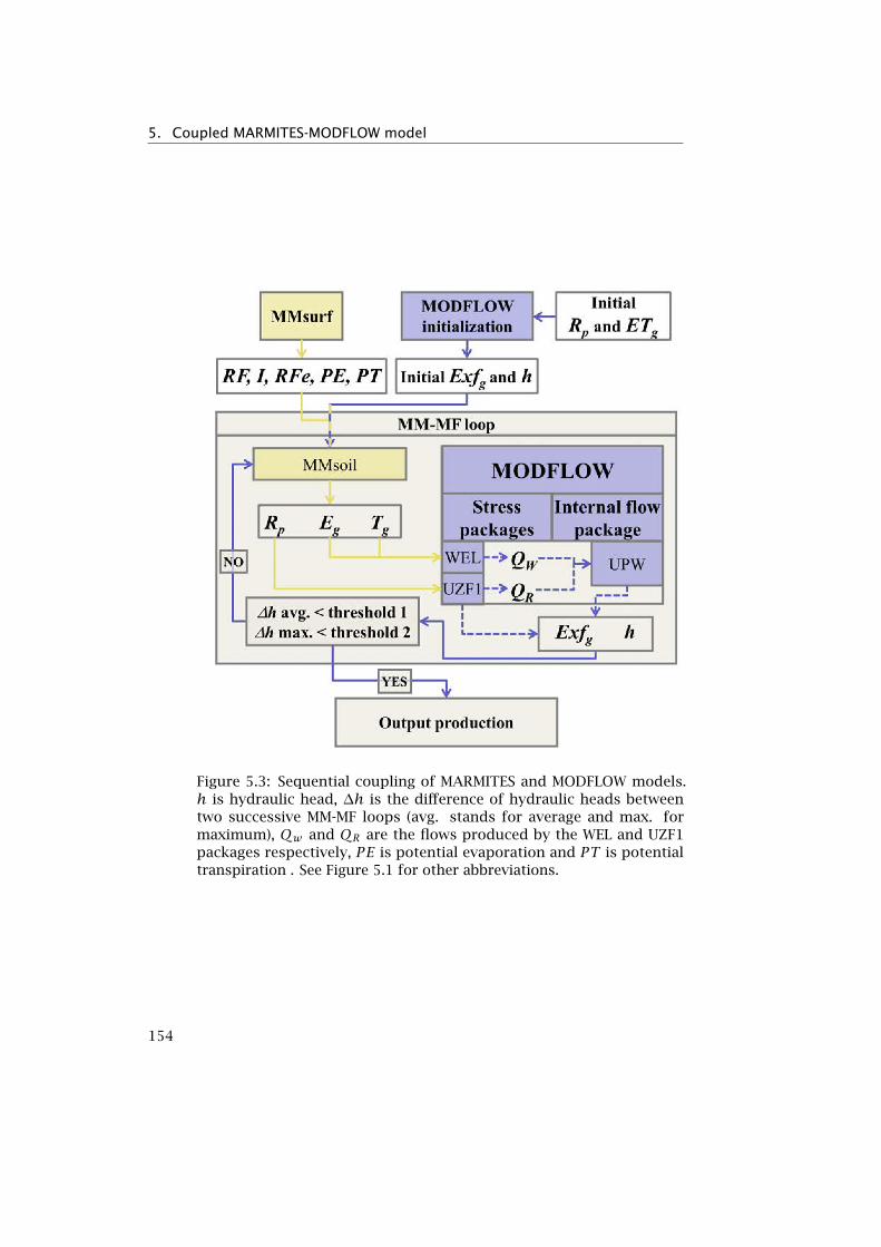
5. Coupled MARMITES-MODFLOW model
Figure 5.3: Sequential coupling of MARMITES and MODFLOW models.h is hydraulic head, ∆h is the difference of hydraulic heads betweentwo successive MM-MF loops (avg. stands for average and max. formaximum), Qw and QR are the flows produced by the WEL and UZF1packages respectively, PE is potential evaporation and PT is potentialtranspiration . See Figure 5.1 for other abbreviations.
154

5.2. Material and Methods
In relation to Eg , Shah et al. (2007) found a soil texture dependentexponential relationships between Eg and the groundwater table depth(d) using numerical simulations of HYDRUS-1D (Šimunek et al., 1998). InMM, their Equation (17) was applied to compute bare soil Eg as following:
Eg/PEg =
1 if d ≤ d′′,y0 + exp−b(d−d
′′) if d > d′′,0 if d ≥ D.
(5.14)
where PEg = PE − Esoil is the groundwater potential evaporation (Esoilis first computed using Equation (5.4)), d′′ is the decoupling depth,y0 is a correction, b is the decay coefficient and D is the extinctiondepth. At depth lower than d′′, PEg is fully satisfied by groundwater, i.e.Eg/PEg = 1. Otherwise the exponential relationship is applied up to theextinction depth D. Equation (5.14) is applied on bare soil using specificset of parameters d′′, b and y0 defined by Shah et al. (2007) for severalsoil texture classes (Table 5.3 and Figure 5.4).
Figure 5.4: Groundwater evaporation (Eg) curves (Equation (5.14)) of themain soil texture classes (after Shah et al., 2007). The soil texture classlabeled "sandy loam field" corresponds to the results of Balugani et al.(2014) obtained from the La Mata catchment. PEg is groundwater poten-tial evaporation and d is groundwater table depth. Refer to Table 5.3 toconsult the corresponding parameters and to section 5.2.1.4 for detailedexplanations.
155

5. Coupled MARMITES-MODFLOW model
Table 5.3: Parameters of equation (5.14) of: (a) standard soil type (Shahet al., 2007); and (b) La Mata catchment soil type (Balugani et al., 2014).d′′ is the decoupling depth (cm), y0 is a correction ([-]), b is the decaycoefficient (cm−1) and D is the extinction depth (cm).
Soil type d′′ y0 b D
sand(a) 16.0 0.000 0.171 50.0
loam(a) 33.0 0.004 0.028 265.0
silt(a) 31.0 0.007 0.021 430.0
clay(a) 45.0 0.006 0.019 620.0
sandy loam field(b) 100.0 0.000 0.013 475.0
The computing of Tg depends first on the root depth (Zr ) definedfor each vegetation type. If the groundwater table depth is higher thanZr , then Tg is set to zero. Otherwise, the following relationships linkingTg to soil moisture (θ) and groundwater potential transpiration (PTg) isapplied:
Tg/PTg =
kTmax if θ = φ,
kTmin +[kTmax − kTmin
][1−
(φ−θφ−θwp
)n]1/nif θwp < θ < φ,
kTmin f θ = θwp,
(5.15)
with
0 < kTmin < kTmax ≤ 1,
where PTg = PT − Tsoil (Tsoil is computed first using Equation (5.5)),kTmin, kTmax and n are vegetation-dependent Tg sourcing parameters,φ is soil porosity and θwp is permanent wilting point. The vegetation-specific sourcing parameters kTmin, kTmax and n allow to control thephreatophytic behavior of the plants by tuning the amount of groundwa-ter that they can uptake, as discussed in section 5.3.1.2.
5.2.1.5 Space and Time Discretization
The catchment is divided into squared-grid cells, all of them with thesame size. Each cell is parametrized with vegetation, soil and aquiferparameters and supports only one soil type but several vegetation typescharacterized by fractional area of their cell occupancy. The time discret-ization is automatically performed by MMsurf based on the rainfall timeseries analysis. For each day with RF > 0 one stress period is definedwhile when there is no rainfall, fluxes are averaged with the period inbetween the two successive events with RF > 0, up to a maximum timeinterval defined by the user (typically 10 days).
156

5.2. Material and Methods
5.2.1.6 Technical Specifications
MM is developed using the Python programming language (version 2.7)and related libraries (SciPy and matplotlib). The code is open source,available at https://code.google.com/p/marmites/. The MF files areimplemented using the FloPy code (Post, 2008), also developed in Python(source code available at https://code.google.com/p/flopy/). Asinput, MM requires 3 types of ASCII files to run. The 1st type corres-ponds to INI files that are required to initialize the 3 MM-MF components(MMsurf, MMsoil and MF). The 2nd file type are ESRI ASCII grid formatmaps of parameters and variables. The 3rd type provides the time seriesof driving forces (meteorological and irrigation data) and state variables(observations). The output spatio-temporal water fluxes are stored in mul-tidimensional grids in HDF5 format (http://www.hdfgroup.org/HDF5/),being automatically exported into ASCII file format at user-defined obser-vations points to allow their import into software such as Microsoft Excelor GoldenSoftware Grapher. MM also produces maps and time series offluxes to visualize the model output (see examples in section 5.3.2).
5.2.2 Model Implementation
5.2.2.1 La Mata Catchment Study Case
This study uses the La Mata catchment (∼4.8 km2, see Figure 5.5), locatedin Western Spain (West of Salamanca), to present the functionality ofthe MM-MF model. The La Mata catchment is a sub-catchment of theSardón catchment (∼80 km2) where extensive research on subsurfacewater fluxes at the catchment scale has been carried out (Lubczynski andGurwin, 2005; Lubczynski, 2009, 2011; Reyes-Acosta and Lubczynski,2013; Balugani et al., 2014; Francés et al., 2014; Hassan et al., 2014). Thiscatchment was selected because of a semi-arid, water-limited environ-ment, negligible groundwater use, availability of monitoring data andshallow groundwater table (∼2 m depth) enhancing Eg , Tg and Exfg .Its granitic rock medium is characterized by large heterogeneity, low tomoderate permeability and low storage, typical of hard rock water scarcecondition.
The La Mata sub-catchment has been equipped with an automaticdata acquisition system (ADAS, located at P0, Figure 5.5) that recordshourly hydro-meteorological variables since 1996. The groundwater tablefluctuation is monitored in one piezometer at the P0 location (automatic,hourly measurement) and at several groundwater-connected ponds (P1to P5, with manual, seasonal measurement). Besides, an 18 m high eddycovariance tower (ECT) (Figure 5.5) was installed at ∼140 m ENE fromthe ADAS between June 2009 and June 2012 to record ET (van der Tol,2012).
157
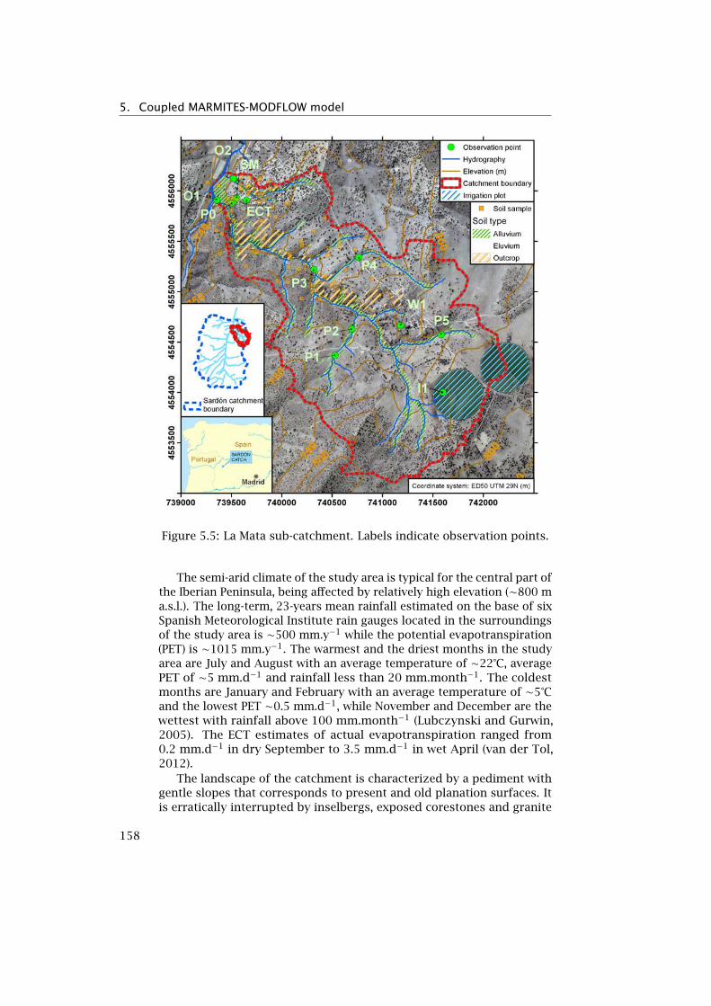
5. Coupled MARMITES-MODFLOW model
Figure 5.5: La Mata sub-catchment. Labels indicate observation points.
The semi-arid climate of the study area is typical for the central part ofthe Iberian Peninsula, being affected by relatively high elevation (∼800 ma.s.l.). The long-term, 23-years mean rainfall estimated on the base of sixSpanish Meteorological Institute rain gauges located in the surroundingsof the study area is ∼500 mm.y−1 while the potential evapotranspiration(PET) is ∼1015 mm.y−1. The warmest and the driest months in the studyarea are July and August with an average temperature of ∼22°C, averagePET of ∼5 mm.d−1 and rainfall less than 20 mm.month−1. The coldestmonths are January and February with an average temperature of ∼5°Cand the lowest PET ∼0.5 mm.d−1, while November and December are thewettest with rainfall above 100 mm.month−1 (Lubczynski and Gurwin,2005). The ECT estimates of actual evapotranspiration ranged from0.2 mm.d−1 in dry September to 3.5 mm.d−1 in wet April (van der Tol,2012).
The landscape of the catchment is characterized by a pediment withgentle slopes that corresponds to present and old planation surfaces. Itis erratically interrupted by inselbergs, exposed corestones and granite
158

5.2. Material and Methods
outcrops. A dense drainage network of incised streams, typical of hardrock catchments, developed along faults. Those are ephemeral streams,with water flowing only in wet season and only after substantial rainfallevents. While the pediment is covered by a thin (0.10 to 0.75 m) sandy-loam inceptisol (eluvium), alluvial deposits 1 to 3 m thick are locatedalong the thalweg (line defining the deepest channel in a valley). The mainpart of the alluvium profile is composed of silty sand above a 0.5 m thicklayer of centimeter to decimeter size pebbles. The shallow subsurfacewas documented by invasive field methods (portable percussion hammerwith sampling gauge, augering and digging). The collected soil sampleswere analyzed in laboratory to retrieve the hydraulic properties and soiltexture.
The land cover consists of sparsely distributed open woodland com-posed of evergreen oak Quercus ilex (Q.i.) subsp. ballota Desf. (Samp.)and broad-leafed deciduous oak Quercus pyrenaica (Q.p.). The canopiesof these two oak trees cover ∼7 % of the La Mata sub-catchment. Theshrub known as Scotch Broom (Cytisus scoparius) is also present locally.The entire area is covered by grasses that sprout in March-May, start towilt in June and next disappear due to the drying soil and cattle grazing.
The groundwater table depth, as monitored in the study area, variesbetween 0.0 and 3.0 m below ground surface (m b.g.s.) along the thal-weg and between 1.0 and 5.0 m b.g.s. at the catchment divides. As thegroundwater system is unconfined, the groundwater table follows the to-pography and is largely influenced by the surficial drainage network. Thegroundwater pattern is natural due to negligible groundwater extraction.
5.2.2.2 Discretization
The spatial discretization of the La Mata sub-catchment was made on aregular square grid of 50 m resolution, corresponding to 60 columns and65 rows. The model simulation was carried out during two successivehydrological years, i.e. from 01/10/2008 to 31/09/2010. According tothe long-term yearly rainfall average of 500 mm.y−1, the first year wasdry, with only 306 mm.y−1 of rainfall, while the second was medium-wet, with 593 mm.y−1. An initialization period was applied between31/05/2008 and 31/09/2008 to allow the model to reach equilibriumunder applied driving forces. The first time step was run in steady-stateconditions, allowing to start the model with average, long-term initialconditions of UZF1 soil moisture and MF hydraulic heads.
5.2.2.3 MM boundary conditions and parametrization
The basic hydro-meteorological variables necessary to obtain the timeseries of driving forces (RF , PE and PT , see section 5.2.1.2 for details)were acquired from the ADAS station. The soil types and granite out-crops were mapped as in Francés and Lubczynski (2011); Francés et al.(2014) using a supervised classification technique applied on two high-resolution, multispectral satellite images: QuickBird from September
159

5. Coupled MARMITES-MODFLOW model
2009 and WorldView-2 from December 2012. The classification methodis based on object-oriented fuzzy-logic analysis (Benz et al., 2004), avail-able in the eCognition software. Two main soil types, i.e. the alluviumand elluvium, were identified and differentiated from granite outcrops(Figure 5.5). The soil data obtained by sampling campaigns (Figure 5.5)and processed in laboratory allowed to retrieve the soil texture and hy-draulic properties (Table 5.4). The lack of sampling at the top of thecatchment is due to the prohibition of the land-owner to access his area.Alfalfa crop growing in March and cropped in October was attributedto the two crop fields located in the eastern part of the La Mata sub-catchment(Figure 5.5). The related irrigation schedule was defined usingthe program CROPWAT v8.0 (Food and Agriculture Organization, 2009).
Table 5.4: Calibrated soil hydraulic properties of the 2 soil types ofLa Mata catchment. φ: porosity, θfc : soil moisture at field capacity,θwp: soil moisture at wilting point, θi: initial soil moisture, Ksat: soilsaturated hydraulic conductivity, Thick: thickness of the soil layer. Unitsin m3.m−3 expect Ksat and Thick, respectively in mm.d−1 and m.
Soil type Layer φ θfc θwp θi Ksat Thick.
Alluvium 1 0.15 0.125 0.075 0.145 1.5 0.75
2 0.19 0.175 0.100 0.190 1.5 0.25
Eluvium 1 0.22 0.150 0.070 0.215 5.0 0.35
2 0.35 0.200 0.125 0.250 3.0 0.15
5.2.2.4 MF boundary conditions and parametrization
Francés et al. (2014) presented a hydrogeological conceptual model ofthe Sardón catchment, to which the La Mata sub-catchment belongs,using a combination of remote sensing, non-invasive hydrogeophysicsand hydrogeological field data acquisition. They identified two mainhydrostratigraphic layers, the saprolite and the fissured layers, thatthey geometrically and parametrically characterized. For the sake ofsimplicity, in the present La Mata case study focused on demonstrationof the MM-MF capability, one aquifer layer schematizing both saproliteand fissured layers was defined.
The La Mata catchment divide was defined as no-flow boundary. Thecatchment outlet was represented using drain (DRN) cells to simulatethe groundwater outflow of the catchment. The parameters required bythe MF model are listed in Table 5.5. The initial hydraulic heads weredefined at the base of the soil layer. Due to the lack of dense, uniformlydistributed piezometric network and small size of the catchment, theaquifer was parametrized with a single value for each of the hydraulicproperty.
160
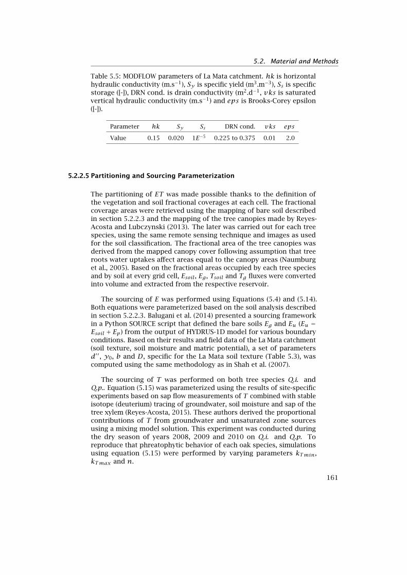
5.2. Material and Methods
Table 5.5: MODFLOW parameters of La Mata catchment. hk is horizontalhydraulic conductivity (m.s−1), Sy is specific yield (m3.m−3), Ss is specificstorage ([-]), DRN cond. is drain conductivity (m2.d−1, vks is saturatedvertical hydraulic conductivity (m.s−1) and eps is Brooks-Corey epsilon([-]).
Parameter hk Sy Ss DRN cond. vks eps
Value 0.15 0.020 1E−5 0.225 to 0.375 0.01 2.0
5.2.2.5 Partitioning and Sourcing Parameterization
The partitioning of ET was made possible thanks to the definition ofthe vegetation and soil fractional coverages at each cell. The fractionalcoverage areas were retrieved using the mapping of bare soil describedin section 5.2.2.3 and the mapping of the tree canopies made by Reyes-Acosta and Lubczynski (2013). The later was carried out for each treespecies, using the same remote sensing technique and images as usedfor the soil classification. The fractional area of the tree canopies wasderived from the mapped canopy cover following assumption that treeroots water uptakes affect areas equal to the canopy areas (Naumburget al., 2005). Based on the fractional areas occupied by each tree speciesand by soil at every grid cell, Esoil, Eg , Tsoil and Tg fluxes were convertedinto volume and extracted from the respective reservoir.
The sourcing of E was performed using Equations (5.4) and (5.14).Both equations were parameterized based on the soil analysis describedin section 5.2.2.3. Balugani et al. (2014) presented a sourcing frameworkin a Python SOURCE script that defined the bare soils Eg and Eu (Eu =Esoil + Ep) from the output of HYDRUS-1D model for various boundaryconditions. Based on their results and field data of the La Mata catchment(soil texture, soil moisture and matric potential), a set of parametersd′′, y0, b and D, specific for the La Mata soil texture (Table 5.3), wascomputed using the same methodology as in Shah et al. (2007).
The sourcing of T was performed on both tree species Q.i. andQ.p.. Equation (5.15) was parameterized using the results of site-specificexperiments based on sap flow measurements of T combined with stableisotope (deuterium) tracing of groundwater, soil moisture and sap of thetree xylem (Reyes-Acosta, 2015). These authors derived the proportionalcontributions of T from groundwater and unsaturated zone sourcesusing a mixing model solution. This experiment was conducted duringthe dry season of years 2008, 2009 and 2010 on Q.i. and Q.p. Toreproduce that phreatophytic behavior of each oak species, simulationsusing equation (5.15) were performed by varying parameters kTmin,kTmax and n.
161

5. Coupled MARMITES-MODFLOW model
5.2.2.6 Calibration
The transient calibration of the MM-MF coupled model was done against:(i) soil moisture in MM; and (ii) hydraulic heads in MF. Two soil moistureprofiles were available in the study area, one located in the alluviumat P0 and the other in the eluvium at SM (Figure 5.5). Hydraulic headswere monitored with automatic water level recorders installed at piezo-meter P0 (∼3 m b.g.s.). Episodic records of the water level measured ingroundwater linked-ponds and in a shallow well (respectively observationpoints P1 to P5 and W, Figure 5.5) were also used for calibration. ETmeasurements from the ECT were also compared with the model output.
The calibration process was carried out first using trial and errormethod and next using the PEST algorithm (Doherty, 2005) to obtain finetuning and parameter uncertainties (not discussed here). Both methodswere used in order to obtain a balanced calibration that produced a mean-ingful water balance and respected the observation data. The MMsoilcomponent was calibrated by updating the soil hydraulic parameters andthickness. The MF model was calibrated on hydraulic conductivity (hk),specific yield (Sy ), DRN conductance, UZF1 vertical saturated hydraulicconductivity and UZF1 epsilon factor (vks and eps respectively, seetable 5.1). In PEST, weighting of the observations was made to ensurerepresentativeness of all observation types in the objective function.
To analyze the goodness of fit between simulated and observed curvesof soil moisture and hydraulic heads, 3 calibration criteria were used(Moriasi et al., 2007): (i) Pearson’s correlation coefficient (r ); (ii) rootmean square error (RMSE); and (iii) ratio of the RMSE to the standarddeviation of the observed heads (RSR). While RMSE and RSR measure thediscrepancy between simulated and observed curves, r shows how wellmodel and observation trends fit each other. The calibration processfocused on minimizing RMSE and RSR and maximizing r . The calibrationcriteria are automatically computed and plotted in MM by the Pythoncode.
5.3 Results and discussion
5.3.1 Partitioning and sourcing of evapotranspiration
The partitioning of ET was implemented at the model cell scale using soiland vegetation fractional area, retrieved using a supervised classificationtechnique applied on high-resolution satellite images. This methodwas very efficient, allowing to map at the catchment scale: (i) differentsoil types, differentiating them from granite outcrop; (ii) canopy shapeand canopy area of every single tree with 90% probability of being wellclassified (Reyes-Acosta and Lubczynski, 2013).
162
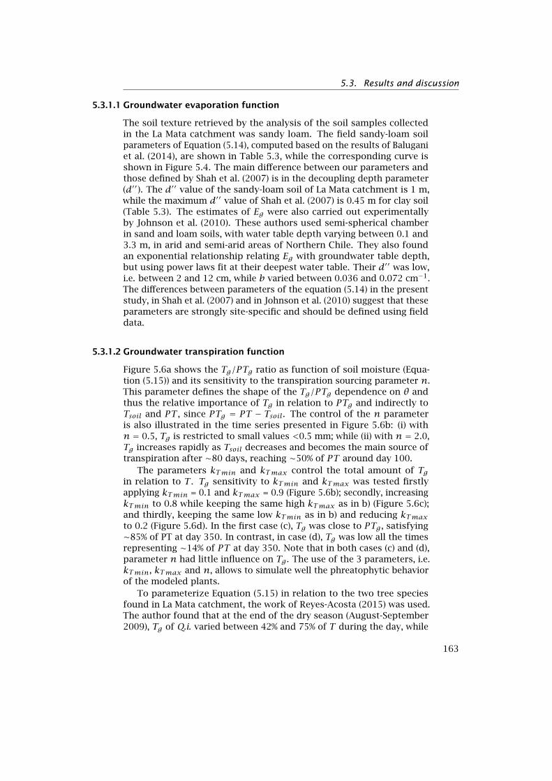
5.3. Results and discussion
5.3.1.1 Groundwater evaporation function
The soil texture retrieved by the analysis of the soil samples collectedin the La Mata catchment was sandy loam. The field sandy-loam soilparameters of Equation (5.14), computed based on the results of Baluganiet al. (2014), are shown in Table 5.3, while the corresponding curve isshown in Figure 5.4. The main difference between our parameters andthose defined by Shah et al. (2007) is in the decoupling depth parameter(d′′). The d′′ value of the sandy-loam soil of La Mata catchment is 1 m,while the maximum d′′ value of Shah et al. (2007) is 0.45 m for clay soil(Table 5.3). The estimates of Eg were also carried out experimentallyby Johnson et al. (2010). These authors used semi-spherical chamberin sand and loam soils, with water table depth varying between 0.1 and3.3 m, in arid and semi-arid areas of Northern Chile. They also foundan exponential relationship relating Eg with groundwater table depth,but using power laws fit at their deepest water table. Their d′′ was low,i.e. between 2 and 12 cm, while b varied between 0.036 and 0.072 cm−1.The differences between parameters of the equation (5.14) in the presentstudy, in Shah et al. (2007) and in Johnson et al. (2010) suggest that theseparameters are strongly site-specific and should be defined using fielddata.
5.3.1.2 Groundwater transpiration function
Figure 5.6a shows the Tg/PTg ratio as function of soil moisture (Equa-tion (5.15)) and its sensitivity to the transpiration sourcing parameter n.This parameter defines the shape of the Tg/PTg dependence on θ andthus the relative importance of Tg in relation to PTg and indirectly toTsoil and PT , since PTg = PT − Tsoil. The control of the n parameteris also illustrated in the time series presented in Figure 5.6b: (i) withn = 0.5, Tg is restricted to small values <0.5 mm; while (ii) with n = 2.0,Tg increases rapidly as Tsoil decreases and becomes the main source oftranspiration after ∼80 days, reaching ∼50% of PT around day 100.
The parameters kTmin and kTmax control the total amount of Tgin relation to T . Tg sensitivity to kTmin and kTmax was tested firstlyapplying kTmin = 0.1 and kTmax = 0.9 (Figure 5.6b); secondly, increasingkTmin to 0.8 while keeping the same high kTmax as in b) (Figure 5.6c);and thirdly, keeping the same low kTmin as in b) and reducing kTmaxto 0.2 (Figure 5.6d). In the first case (c), Tg was close to PTg , satisfying∼85% of PT at day 350. In contrast, in case (d), Tg was low all the timesrepresenting ∼14% of PT at day 350. Note that in both cases (c) and (d),parameter n had little influence on Tg . The use of the 3 parameters, i.e.kTmin, kTmax and n, allows to simulate well the phreatophytic behaviorof the modeled plants.
To parameterize Equation (5.15) in relation to the two tree speciesfound in La Mata catchment, the work of Reyes-Acosta (2015) was used.The author found that at the end of the dry season (August-September2009), Tg of Q.i. varied between 42% and 75% of T during the day, while
163

5. Coupled MARMITES-MODFLOW model
Tg of Q.p. varied between 25 and 35% of T . To obtain the same Tg/Tproportion as experimentally estimated, we defined the transpirationsourcing parameters presented in Table 5.6 for the two tree species. Suchparameters were also defined for the non-phreatophytic alfalfa crop andgrass, ensuring that Tg was null or negligible.
Table 5.6: Vegetation parameters of equation (5.15) defined for theLa Mata catchment. kTmin, kTmax and n are vegetation-dependent Tgsourcing parameters (unitless) and Zr is root depth (m).
Veg. type kTmin kTmax n Zr
Q.i. 0.10 0.80 2.0 15.0
Q.p. 0.50 0.90 2.0 10.0
Grass 0.01 0.02 0.5 0.4
Alfalfa 0.01 0.02 0.5 1.2
164
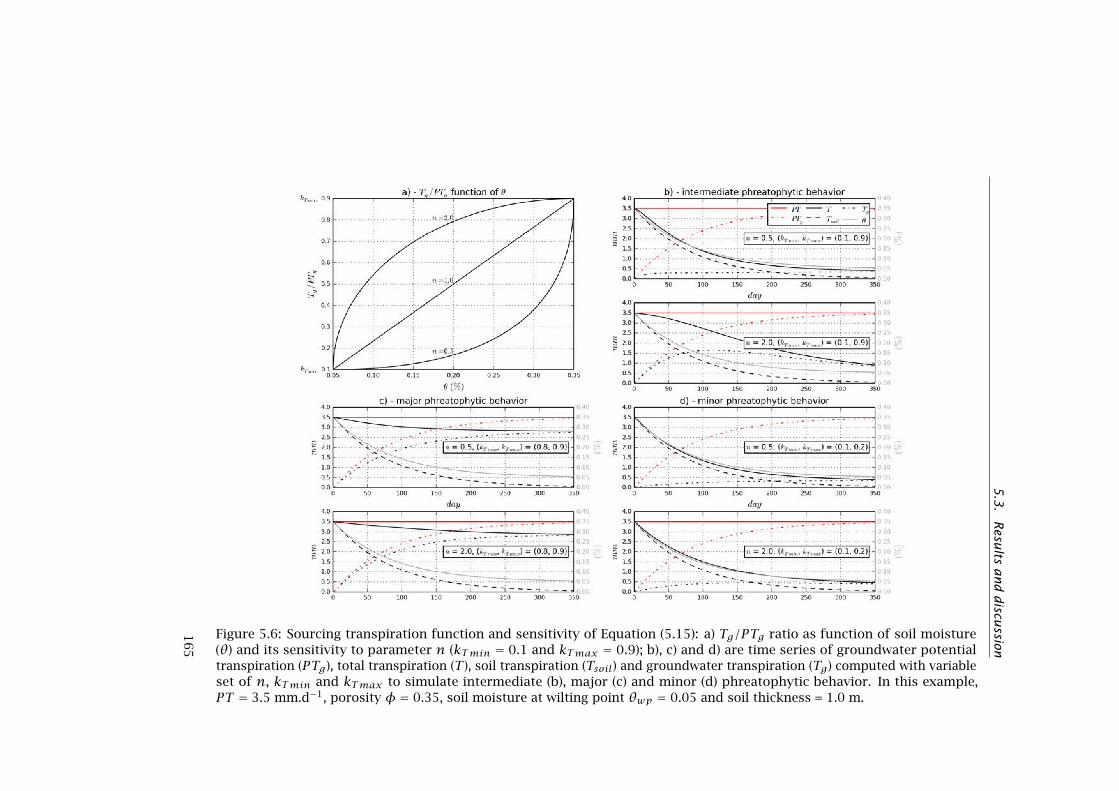
5.3
.R
esults
and
discu
ssion
Figure 5.6: Sourcing transpiration function and sensitivity of Equation (5.15): a) Tg/PTg ratio as function of soil moisture(θ) and its sensitivity to parameter n (kTmin = 0.1 and kTmax = 0.9); b), c) and d) are time series of groundwater potentialtranspiration (PTg), total transpiration (T ), soil transpiration (Tsoil) and groundwater transpiration (Tg) computed with variableset of n, kTmin and kTmax to simulate intermediate (b), major (c) and minor (d) phreatophytic behavior. In this example,PT = 3.5 mm.d−1, porosity φ = 0.35, soil moisture at wilting point θwp = 0.05 and soil thickness = 1.0 m.
16
5

5. Coupled MARMITES-MODFLOW model
The Tg solution proposed in this study based on Equation (5.15) isgroundwater table depth independent but driven by climatic conditionsand soil moisture availability. The only study of that type which pro-posed partitioning of transpiration is by Baird and Maddock III (2005).However, they proposed different transpiration-related approach. Theydeveloped a MF package to compute riparian Tg based on plant physiolo-gical characteristics, applying a bell-shaped Tg relation with GWTD thatrequires vegetation specific parameters. That solution was developed forriparian and wetland ecosystems, i.e. environments with very shallowwater table frequently rising above the land surface and creating unfavor-able anaerobic conditions leading to a T reduction and dead of the plantby anoxia. The bell-shaped function, developed for such ecosystems,reflects well this behavior by simulating a Tg decline that follows thewater rise to the surface. However, it is questionable if their solution isapplicable to open oak woodland ecosystems or any other ecosystemscharacterized by deeply rooted trees with access to both unsaturatedand saturated zones reservoirs. For such settings, it is assumed in thisstudy that if a tree is phreatophytic, i.e. have roots deep enough to beable to tap groundwater, and if soil moisture is not sufficient to fulfillthe tree water demand, then Tg occurs with rate independent on GWTD(equation (5.15)). This assumption is in agreement with experimentalresults of Balugani et al. (2015) who partitioned and sourced ET basedon field measurements (ECT, sap flow, soil moisture, groundwater level,isotopes tracing) and HYDRUS modeling. They found an almost invarianttranspiration rate during late spring and summer period, while the soilmoisture was progressively depleted and the water table dropped morethan 1 m (maximum GWTD was 3 m). Throughout that period, T wasstable because the decrease of Tsoil was compensated by the increaseof Tg . That increase took place despite lowering of water table, whichconfirmed that water table depth had no or negligible influence on Tgand that the trees are adapted to tap water from any accessible reservoirin order to satisfy the transpiration requirements. These results are inagreement with several other studies such as David et al. (2004); Paçoet al. (2009); Miller et al. (2010) that independently found that oak trees insavanna environment could compensate low soil moisture in dry seasonby taping groundwater at depth of 8 and 13 m. These authors also foundthat groundwater uptake was thermodynamically favorable over soilwater uptake during dry seasons and that such behavior was compatiblewith the tree physiology. However, as the transpiration rates were belowthe atmospheric water demand, groundwater uptake constitutes a treestrategy to subsist during dry season and not a mechanism for continuedplant growth.
5.3.2 MM-MF output and case study results
The capability and potential of the MM-MF model are presented onthe base of the real case study simulation of the surface groundwaterinteractions in the La Mata catchment in Spain for hydrological years
166

5.3. Results and discussion
from October 2008 to September 2010 (respectively called from hereonwards as 1st and 2nd year). The calibrated time series and calibrationcriteria relative to soil moisture and hydraulic heads at observationpoints P0 and SM are respectively shown in Figure 5.7 and Table 5.7.The fitting between simulated and observed curves of soil moisture ischaracterized by relatively high r varying between 0.7 and 0.8. RSRand RMSE are also satisfactory, indicating small deviation in relation toobserved data. The hydraulic head at P0 is also well calibrated, respectingthe trend and amplitude of the observed data. Its relatively low r = 0.5and high RMSE = 0.7 m can be explained by a temporal shift betweensimulated and observed data. The calibration also ensured consistentsimulated water levels at the catchment outlet (O1 and O2) and at theponds (P1 to P5) in relation to the observed values (Figures S7 to S18).The model simulations of ET time series are also in agreement withmeasurements at the ECT (Figure 5.8). The simulated daily ET variedbetween 0.05 mm (October 2009) and 2.1 mm (July 2010), which iswithin the range and shows the same trend as ET measured by the ECtower (van der Tol, 2012). However, the measured ET amplitude waslarger than the simulated ET because the ET measurements at the ETtower correspond to acquisition of almost instantaneous values whileET computed by MM was based on daily simulation.
Table 5.7: Calibration criteria results on soil moisture and hydraulicheads. r is the Pearson’s correlation coefficient (unitless values varyingbetween 0 and 1), RMSE is the root mean square error (m3.m−3 for soilmoisture and m for heads) and RSR is the ratio of RMSE to the standarddeviation of the observed heads (unitless).
Obs. pt. State variable r RMSE RSR
P0 soil. moist layer 1 0.73 0.190 0.78
soil. moist layer 2 0.82 0.220 0.66
heads MF layer 1 0.49 0.660 1.04
SM soil. moist layer 1 0.83 0.025 0.62
soil. moist layer 2 0.77 0.043 0.75
Daily time series of simulated surface and subsurface fluxes aver-aged at the catchment scale are presented in Figure 5.9. The 1st plotfrom the top shows the daily rainfall (RF ) and rainfall excess (RFe, seeEquation (5.1)). As interception in the study area was low due to the lowspatial coverage of the trees (∼7%) and low storage capacity of alfalfacrops and grass, RFe differs very little from RF . The 2nd plot showssurface runoff (Ro), infiltration into soil (Inf ) and other surface waterfluxes. Significant Ro occurred only during the 2nd, wet hydrologicalyear, which is in agreement with the field observations. Note that surfacewater is not routed in the current version of the MM-MF model, thusthe simulated runoff is instantaneous. In such a small catchment as La
167

5. Coupled MARMITES-MODFLOW model
Figure 5.7: Observed (dot curves) and simulated (line curves) soil mois-ture and groundwater table depth time series at SM (top) and P0 (middleand bottom) observation points. Location of SM and P0 points in Fig-ure 5.5. Soil moisture: θn obs is observed soil moisture in the field, θnis simulated soil moisture and n is the soil layer index varying between1 and the total number of soil layers (in this case 2). Groundwater tabledepth: d obs is observed hydraulic head in the field, dn is simulatedhydraulic head, d corr is simulated hydraulic head corrected to takeinto account saturated soil layers and n is the MF layer index varyingbetween 1 and the total number of soil layers (in this case 1).
Figure 5.8: ET observed at the eddy covariance tower (ECT) and simulatedby MM-MF (MM). Rainfall (RF ) is also indicated.
168

5.3. Results and discussion
Mata, the routing is not very relevant because the residence time in thestreams is short, i.e. less than one day, although in bigger catchmentsthis limitation should be resolved. The 3rd plot shows the evaporationfluxes, i.e. soil evaporation (Esoil) and groundwater evaporation (Eg),together with potential evaporation (PE). The 4th is similar, but for tran-spiration, i.e. soil transpiration (Tsoil), groundwater transpiration (Tg)and potential transpiration (PT ). During the two dry seasons neither PEnor PT were satisfied, despite the contribution of groundwater. In the 1st
year, E reached maximally 1.0 mm.d−1 while in the 2nd year 1.5 mm.d−1,both at the peak of the dry season. The T contribution to ET was muchlower than E, showing a maximum of 0.4 mm.d−1. This is due to the lowvegetation coverage in the catchment, which also explains the low valueof Tg (maximum of 0.1 mm.d−1) and relatively high Eg (0.5 mm.d−1 inJuly-August 2010). Comparing the two years analyzed, E, T , Esoil, Tsoiland Eg were larger in the 2nd year than in the 1st year because of higherRF . Exception was Tg that was pretty similar in both years, despite thewater table in the 1st year was deeper than in the 2nd (Figure 5.7). Thisbehavior was expected due to the Tg independence on GWTD implemen-ted in equation (5.15). Percolation (Rp), gross recharge (Rg), groundwaterexfiltration (Exfg) and groundwater evapotranspiration (ETg) are shownin the last, 5th plot of Figure 5.9. Note that the difference between Rgand Rp is attributed to percolation zone storage. Rg occurred betweenDecember and May, reaching a maximum of 2 mm.d−1 in January 2010.Rg is only slightly delayed in relation to Rp, due to shallow water tablecondition and related short travel time across the percolation zone. Exfgis more delayed, indicating a subsurface travel time from the rechargearea to the discharge area of around one month.
The yearly, catchment scale water balances over each hydrologicalyear are presented in Figure 5.10 as 2 Sankey diagrams. Yearly Esoil in1st and 2nd year were 139 and 175 mm respectively, which represented45 and 29 % of RF . Yearly Eg was constant during both years with avalue of 38 mm, corresponding to 12 and 6% of RF , representing animportant water balance component, in particular during the 1st dry year.Tg showed the same tendency, but with lower values due to the earliermentioned low catchment vegetation coverage. As expected, Ro waslower in the 1st year than in the 2nd, with a value of 63 mm in the 1st year,i.e. 21% of RF , and 241 mm in the 2nd, i.e. 41% of RF . Rg was 88 mm.y−1
in the 1st and 169 mm.y−1 in the 2nd year, in both cases representing 29%of RF . In contrast to stable Rg, Rn = Rg−ETg−Exfg was quite differentin both years: in the 1st, dry year, Rn was negative (-15 mm) while inthe 2nd, wet year was positive (22 mm). Groundwater storage change(∆Sg) had similar tendency, loosing 22 mm in the 1st year and gaining15 mm the 2nd. Despite two years with totally different rainfall, thegroundwater outflow of the catchment (DRN) remained nearly the same,which confirms a limited system storage capacity and the predominanceof evapotranspiration and/or exfiltration processes.
The spatial variability of water fluxes can be visualized in MM-MF asfor example in the maps of Figures 5.11-5.13. These maps show selected
169
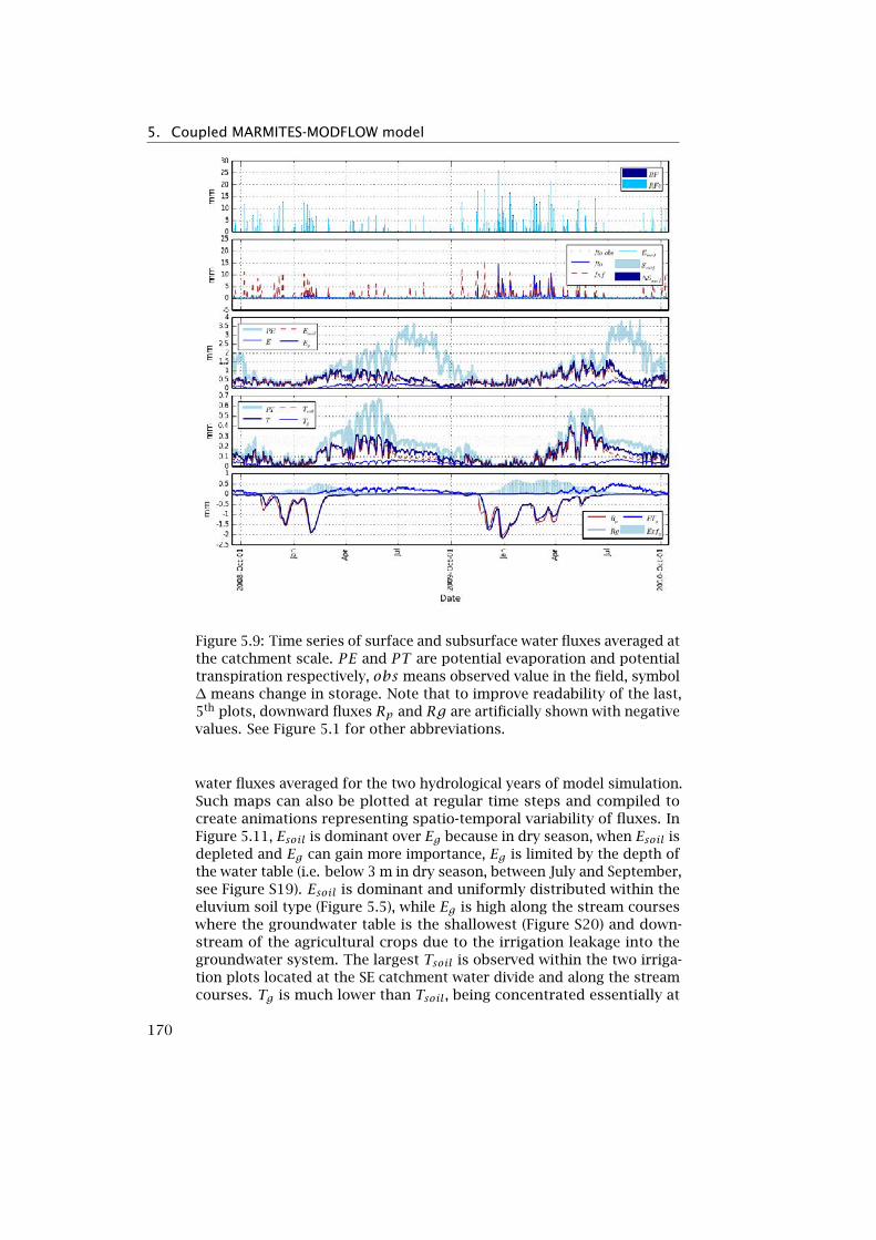
5. Coupled MARMITES-MODFLOW model
Figure 5.9: Time series of surface and subsurface water fluxes averaged atthe catchment scale. PE and PT are potential evaporation and potentialtranspiration respectively, obs means observed value in the field, symbol∆ means change in storage. Note that to improve readability of the last,5th plots, downward fluxes Rp and Rg are artificially shown with negativevalues. See Figure 5.1 for other abbreviations.
water fluxes averaged for the two hydrological years of model simulation.Such maps can also be plotted at regular time steps and compiled tocreate animations representing spatio-temporal variability of fluxes. InFigure 5.11, Esoil is dominant over Eg because in dry season, when Esoil isdepleted and Eg can gain more importance, Eg is limited by the depth ofthe water table (i.e. below 3 m in dry season, between July and September,see Figure S19). Esoil is dominant and uniformly distributed within theeluvium soil type (Figure 5.5), while Eg is high along the stream courseswhere the groundwater table is the shallowest (Figure S20) and down-stream of the agricultural crops due to the irrigation leakage into thegroundwater system. The largest Tsoil is observed within the two irriga-tion plots located at the SE catchment water divide and along the streamcourses. Tg is much lower than Tsoil, being concentrated essentially at
170

5.3. Results and discussion
SE of the catchment where the density of trees is the highest (Figure S5).Finally, Figure 5.13 (left) shows the spatial distribution of the net re-charge, separating catchment into recharge areas (Rn > 0, bluish color)and discharge areas (Rn < 0, reddish color). Figure 5.13 (right) presentsthe spatial distribution of groundwater exfiltration, closely related to Ro(Figure S21) and concentrated along the streams, showing the dynamicrelationship between surface and groundwater in the catchment.
171
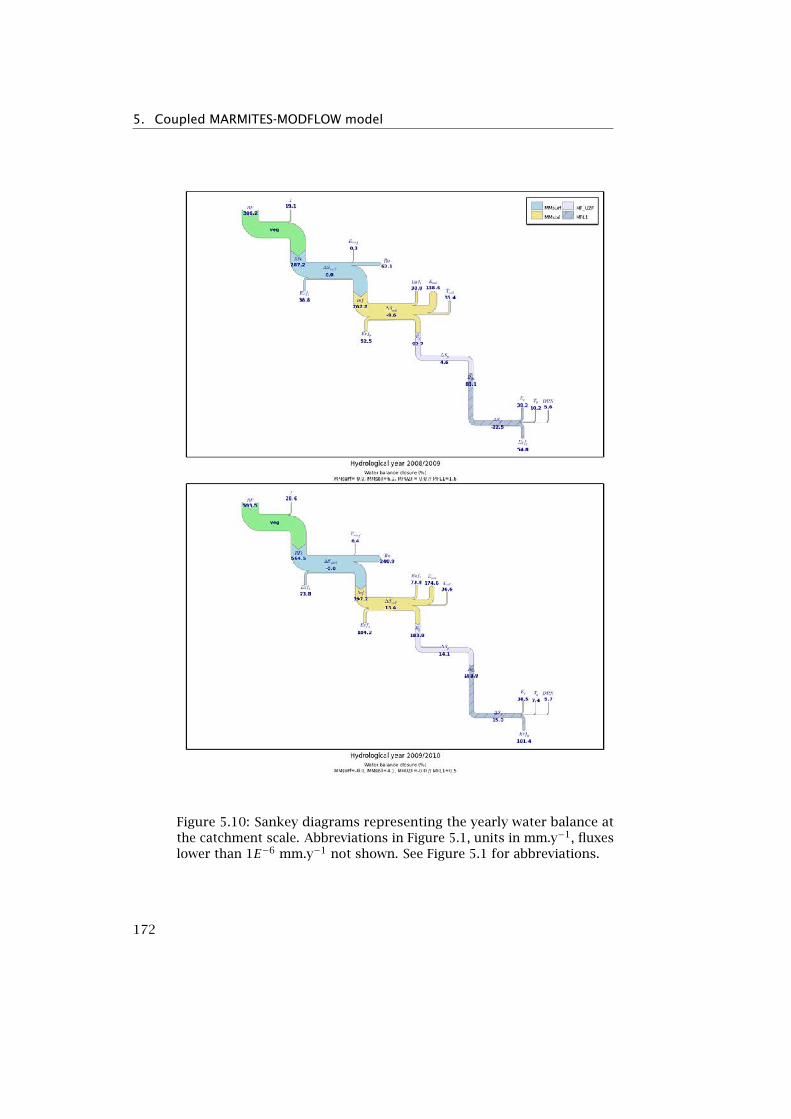
5. Coupled MARMITES-MODFLOW model
Figure 5.10: Sankey diagrams representing the yearly water balance atthe catchment scale. Abbreviations in Figure 5.1, units in mm.y−1, fluxeslower than 1E−6 mm.y−1 not shown. See Figure 5.1 for abbreviations.
172

5.3
.R
esults
and
discu
ssion
Figure 5.11: Two-year average of soil evaporation (Esoil, on the left) and groundwater evaporation (Eg , on the right). Note thateach map has its own color scale.
17
3

5.
Coupled
MA
RM
ITES-M
OD
FLOW
model
Figure 5.12: Two-year average of soil transpiration (Tsoil, on the left) and groundwater transpiration (Tg , on the right). Notethat each map has its own color scale.
17
4

5.3
.R
esults
and
discu
ssion
Figure 5.13: Two-year average groundwater net recharge (Rn, on the left) and groundwater exfiltration (Exfg , on the right).Note that each map has its own color scale.
17
5

5. Coupled MARMITES-MODFLOW model
5.3.3 Comparison with other studies
In parallel work to this study, Balugani et al. (2015) implemented experi-mentally the partitioning and sourcing of evaporation and transpiration,also in the same La Mata catchment. The study was carried out duringthe dry season between days 29 of July and 7 of September of years 2009and 2010, i.e. when grass was dormant so could be excluded from ETcalculation. The following ET fluxes were quantified within the footprintarea of the ECT: (i) total ET based on EC tower measurement (van derTol, 2012); (ii) tree transpiration (T ) by remote sensing upscaling ofsap flow measurements (Reyes-Acosta and Lubczynski, 2013), furthersourced into Tu and Tg based on stable isotopes experiments (Reyes-Acosta, 2015); and (iii) bare soil evaporation (E) sourced into Eu and Egbased on soil texture and HYDRUS-SOURCE modeling (Balugani et al.,2014) using data from soil profiles of temperature, moisture and matricpotential. The four components obtained as a result of experimentalpartitioning and sourcing of ET (Eu, Eg , Tu and Tg) were compared withthe EC tower estimates of the total ET , that we also compared in thisstudy with the MM-MF modeled fluxes (Esoil, Eg , Tsoil, Tg , see Table 5.8).The results showed a good agreement, particularly in year 2009, betweenexperimentally partitioned and sourced fluxes and the correspondingMM-MF modeled ET fluxes, as well as between ET experimental, MM-MFmodeled and measured by the EC tower. The partitioning and sourcingresults confirmed the large importance of groundwater evaporation insavannah type of environments as La Mata oak woodland study area.Moreover, the consistency between the results of the 3 methods is afavorable indicator of the good quality of the fluxes assessment by theMM-MF modeling approaches.
176
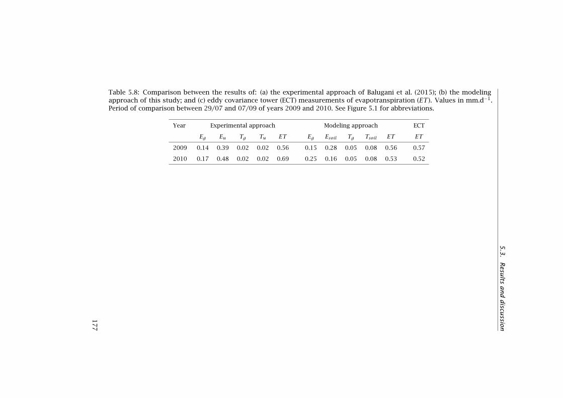
5.3
.R
esults
and
discu
ssion
Table 5.8: Comparison between the results of: (a) the experimental approach of Balugani et al. (2015); (b) the modelingapproach of this study; and (c) eddy covariance tower (ECT) measurements of evapotranspiration (ET ). Values in mm.d−1.Period of comparison between 29/07 and 07/09 of years 2009 and 2010. See Figure 5.1 for abbreviations.
Year Experimental approach Modeling approach ECT
Eg Eu Tg Tu ET Eg Esoil Tg Tsoil ET ET
2009 0.14 0.39 0.02 0.02 0.56 0.15 0.28 0.05 0.08 0.56 0.57
2010 0.17 0.48 0.02 0.02 0.69 0.25 0.16 0.05 0.08 0.53 0.52
17
7

5. Coupled MARMITES-MODFLOW model
Subsurface water fluxes in the Sardón area, which includes La Matacatchment, were recently assessed by Hassan et al. (2014) using thetransient, distributed GSFLOW model (Markstrom et al., 2008). As thereis a relative uniformity of geology, soil, land use and climatic conditionsbetween the two areas, and because GSFLOW is likely the most similarto MM-MF code, the results of both models could be compared. Ingeneral, there is a good agreement between the two models, particularlyin ET and Rn fluxes assessment. A relevant results of the GSFLOWsolution was that ETp was found to be negligible (mean of 18 years was1.14 mm.y−1), which justified the exclusion of the ETp option in MM-MFfor the hydrogeological settings of this study. However, in areas withseveral meters thick unsaturated zone, e.g. the Kalahari Desert, ETpmay be a significant component of the water balance (Lubczynski, 2009,2011), so for such simulations appropriate MM-MF coding adjustmenthave to be added.
5.3.4 Model Performance
The run time of MM applied to the La Mata catchment at daily timestep took about 2 min for MMsurf, 42 min for MMsoil, 4 min for MF(PC with Intel®Core™2 Duo CPU @2.40GHz, 4GB RAM). The code of theMM model in general and the module MMsoil in particular are based onconditions (if...then...else) to test the state of the soil reservoir (saturatedor not) and its relation with the groundwater reservoir (percolation orexfiltration). Due to these conditions, the code is much slower to solvethe equations than a numerical scheme based on matrix computing. TheMM running time is comparable to other models with similar structureas for instance INFIL or GSFLOW. Note that MF running time may besignificantly increased while using the UZF1 package if the groundwaterlevels rise above land surface in a large number of model cells. This isdue to the additional calculations required to compute the groundwaterdischarge to the land surface (Niswonger et al., 2006).
Due to the sequential coupling that obliges to run MM-MF repetitivelyuntil the head difference between two successive runs is less than a user-defined threshold (Figure 5.3), the total run time of the MM-MF modelis pretty long. In general 3 or 5 MM-MF loops are sufficient to reachequilibrium, which requires a full run time of 138 to 230 min. This timecould be drastically reduced by running sequentially MM and MF at eachtime step, but it requires the recording of UZF1 soil moisture profilesat each cell to be used as initial condition for the next time step, whichis not possible in the current version of UZF1. Another possibility is toimplement a full coupling of MM and MF by rewriting MM in FORTRANand integrate MM as MF package.
178
5.4. Conclusions
5.4 Conclusions
This study presented a two-way coupled model that computes spatio-temporally the surface and subsurface fluxes at the catchment scale.The coupled model is composed of the novel water balance model ofthe soil zone, MARMITES, and USGS MODFLOW-NWT code. The noveltyof the proposed solution resides in the implementation of partitioningand sourcing of the evapotranspiration fluxes. In particular, a novelfunction based on soil moisture availability and transpiration demanddriven by climatic conditions is proposed to quantify the groundwatertranspiration (Tg). The computing of groundwater evaporation (Eg) onbare soils was implemented following the methodology proposed byShah et al. (2007).
The model was applied to the small La Mata catchment (Spain), char-acterized by water limited environment, and calibrated against statevariables of the soil and saturated zones (soil moisture and hydraulicheads respectively). The results showed the importance of Eg , larger inthe first, dry year (12.5% of RF ) and smaller in the second, wetter year(6.5% of RF ). Also Tg was larger in dry year than in the wet but withgenerally much lower values (3.3% of RF and 1.2% of RF respectively)than Eg because of low vegetation coverage. Considering seasonal vari-ability, Eg and Tg were the largest in dry seasons when soil moisturewas the most depleted. This points at regulating role of groundwaterfluxes and predominant role of climate as driving force of E and T . Arelevant aspect with respect to transpiration was also that during bothdry seasons the T/PT ratio was almost constant when the decline ofsoil moisture and Tsoil were compensated by increase of Tg occurringsimultaneously with decline of water table. This indicates that once treeroots have access to groundwater, Tg is then independent (or negligiblydependent) on water table fluctuation and that the trees can tap waterinterchangeably from any accessible reservoir in order to satisfy thetranspiration requirements driven by the climatic conditions. This beha-vior reproduced well the results of experimental studies carried out inthe same area (van der Tol, 2012; Reyes-Acosta and Lubczynski, 2013;Balugani et al., 2014) and is in agreement with other studies performedin other, similar open oak woodland ecosystems (David et al., 2004; Paçoet al., 2009; Miller et al., 2010).
The MM-MF model constitutes an effective tool to integrate at thecatchment scale surface, unsaturated zone and groundwater fluxes and toprovide a detailed, spatio-temporal water balance, including partitioningand sourcing of ET . The MM-MF allows also for easy integration ofthe results of local experimental studies to calibrate or validate modelsimulation. The specific ability of MM-MF model to partition and sourcesubsurface fluxes constitutes a particularly valuable and novel modelingoption to analyze the role of tree water uptake and bare soil evaporationin hydrology, particularly in water limited environments. Such option isexpected to be a critical support for water management, particularly in
179

5. Coupled MARMITES-MODFLOW model
assessing the impact of climate and land cover changes on groundwaterresources and for mapping groundwater dependent ecosystems.
180
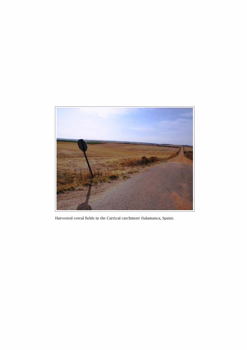
Harvested cereal fields in the Carrizal catchment (Salamanca, Spain).


6Integrating MRS data withhydrologic model - CarrizalCatchment (Spain)
6.1 Introduction
In the last decades groundwater became widely used for water supplybecause of its better quality as compared to surface water and because ofreduction of water abstraction cost (Llamas and Martínez-Santos, 2005).However the prospection and quantification of groundwater is difficultdue to subsurface heterogeneity. An improvement in the efficiency ofevaluation and management of groundwater resources is needed tomitigate the increasing pressure of the demand, particularly in arid andsemi-arid water limited environments.
For quantification of groundwater resources at the catchment scale,distributed numerical hydrological models are considered optimal. How-ever, to provide a valuable management tool, such models need appro-priate acquisition of reliable spatial and temporal input data (Lubczynskiand Gurwin, 2005; Lubczynski, 2011). A classic way to gather subsurfaceparameters to set up hydrological models is through borehole drillingand pumping tests. However, that method is invasive, expensive and timeconsuming. Non-invasive hydrogeophysical methods allow to comple-ment the invasive methods, in efficient and economically sound way. Theapplication of such methods as a support for catchment scale, distrib-uted hydrogeological models has recently received significant attention.Dam and Christensen (2003) demonstrated that an improvement of the
This chapter is based on: Integrating MRS data with hydrologic model Car-rizal catchment (Spain). Baroncini-Turricchia, G., A. P. Francés, M. W. Lubczyn-ski, J. Martínez-Fernández, and J. Roy (2014), Near Surface Geophysics, 12, doi:10.3997/18730604.2014003. The author of this thesis participated or realized thefollowing tasks: (i) acquisition and processing of magnetic and MRS data; (ii) writing ofthe geological description; (iii) development of the MARMITES model and its coupling withMODFLOW (see Chapter 5); (iv) writing of the MARMITES-MODFLOW model description;(v) model calibration; (vi) revision of the manuscript.
183

6. Integrating MRS data with hydrologic model
hydraulic conductivity field is possible using non-invasive techniquesbut depends on number, location and uncertainty of the geophysicalobservations. The disadvantage of classical non-invasive geophysicaltechniques is that they often cannot be used as a straightforward supportfor hydrogeological models. For instance Andersen et al. (2012) showedthat relying on transient electromagnetic (TEM) can lead to different in-terpretations of hydrogeology of buried valleys when different inversionprocesses are applied. This is the main reason that many researchers,except of exploration purpose, apply nowadays classical, non-invasivehydrogeophysics only for qualitative assessment, to interpret the realitywith the aim of building conceptual hydrogeological models. For example,an integrated study of Francese et al. (2009), combining geological datawith three-dimensional resistivity tomography and shallow seismic sur-veys, was carried out in fractured sandstone aquifer in Tuscany (Italy)to assess interrelation between tectonics and groundwater circulation.In the northern Matabeleland (Zimbabwe), TEM and continuous verticalelectrical sounding (CVES) were used to upgrade the hydrogeologicalconceptual model: CVES was applied to define the near surface geo-logical structures and TEM to define the deeper structures (Danielsenet al., 2007). In Okavango Delta (Botswana), time domain electromagneticmethod (TDEM) was used to study three dimensional salinity anomalies(Bauer-Gottwein et al., 2010) otherwise difficult to define and interpret.In the Föhr Island (Germany) airborne electromagnetics (SkyTEM) andseismic reflections were compiled into a 3D model (Burschil et al., 2012)that was meant as a basis for a groundwater flow model. In Denmark,a strong effort in near-surface geophysical data integration resulted indevelopment of Sequential Hydrogeophysical Inversion (SHI), in whichinverted geophysical models provided information for hydrologic models(Herckenrath, 2012).
In contrast to classical geophysical methods, the magnetic resonancesounding (MRS) is the only geophysical method that can provide quantit-ative assessment of water in subsurface. Through assessment of signalamplitude, the MRS is sensitive to the quantity of water in subsurfaceand through the signal decay, to permeability of the medium in whichthe subsurface water is stored and flows. The MRS technique is alreadyknown and well accepted as non-invasive, quantitative evaluation ofwater in subsurface rather than prospecting hydrogeophysical tool. Moreinformation about principles of the MRS technique with emphasis onquantification of groundwater resources can be found in: Lubczynskiand Roy (2003); Roy and Lubczynski (2003); Lubczynski and Roy (2004,2007); Plata and Rubio (2007, 2008); the parameterization of aquifers inLubczynski and Roy (2005, 2007); Vouillamoz et al. (2007); Boucher et al.(2009b); Vouillamoz et al. (2012b); and parameterization of unsaturatedzone in Roy and Lubczynski (2005); Mohnke and Yaramanci (2008); Walshet al. (2014).
The ability of MRS to retrieve the subsurface flow and storage para-meters of hydrological systems makes it suitable not only for site-specificstudies but also for distributed modeling studies, for example focusing
184
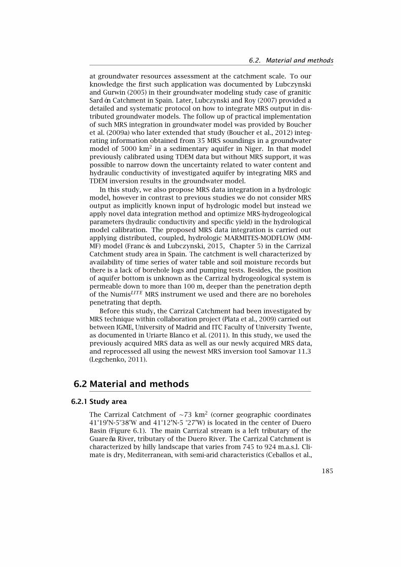
6.2. Material and methods
at groundwater resources assessment at the catchment scale. To ourknowledge the first such application was documented by Lubczynskiand Gurwin (2005) in their groundwater modeling study case of graniticSardón Catchment in Spain. Later, Lubczynski and Roy (2007) provided adetailed and systematic protocol on how to integrate MRS output in dis-tributed groundwater models. The follow up of practical implementationof such MRS integration in groundwater model was provided by Boucheret al. (2009a) who later extended that study (Boucher et al., 2012) integ-rating information obtained from 35 MRS soundings in a groundwatermodel of 5000 km2 in a sedimentary aquifer in Niger. In that modelpreviously calibrated using TDEM data but without MRS support, it waspossible to narrow down the uncertainty related to water content andhydraulic conductivity of investigated aquifer by integrating MRS andTDEM inversion results in the groundwater model.
In this study, we also propose MRS data integration in a hydrologicmodel, however in contrast to previous studies we do not consider MRSoutput as implicitly known input of hydrologic model but instead weapply novel data integration method and optimize MRS-hydrogeologicalparameters (hydraulic conductivity and specific yield) in the hydrologicalmodel calibration. The proposed MRS data integration is carried outapplying distributed, coupled, hydrologic MARMITES-MODFLOW (MM-MF) model (Francés and Lubczynski, 2015, Chapter 5) in the CarrizalCatchment study area in Spain. The catchment is well characterized byavailability of time series of water table and soil moisture records butthere is a lack of borehole logs and pumping tests. Besides, the positionof aquifer bottom is unknown as the Carrizal hydrogeological system ispermeable down to more than 100 m, deeper than the penetration depthof the NumisLITE MRS instrument we used and there are no boreholespenetrating that depth.
Before this study, the Carrizal Catchment had been investigated byMRS technique within collaboration project (Plata et al., 2009) carried outbetween IGME, University of Madrid and ITC Faculty of University Twente,as documented in Uriarte Blanco et al. (2011). In this study, we used thepreviously acquired MRS data as well as our newly acquired MRS data,and reprocessed all using the newest MRS inversion tool Samovar 11.3(Legchenko, 2011).
6.2 Material and methods
6.2.1 Study area
The Carrizal Catchment of ∼73 km2 (corner geographic coordinates41°19’N-5°38’W and 41°12’N-5 °27’W) is located in the center of DueroBasin (Figure 6.1). The main Carrizal stream is a left tributary of theGuareña River, tributary of the Duero River. The Carrizal Catchment ischaracterized by hilly landscape that varies from 745 to 924 m.a.s.l. Cli-mate is dry, Mediterranean, with semi-arid characteristics (Ceballos et al.,
185

6. Integrating MRS data with hydrologic model
2002), precipitation of 485 mm.y−1 and FAO 56 Reference Evapotran-spiration (Allen et al., 1998) of 1093 mm.y−1, as measured at Villamorweather station. The Carrizal Catchment belongs to the REMEDHUSSoil Moisture Network of Salamanca University (Martínez-Fernández andCeballos, 2005).
Figure 6.1: Geology of the study area (Instituto Geológico y Minerode España, 1978, 2000): T1 - Cabrerizos Sandstones (Middle Eocene -Oligocene), silts and sandstones with conglomeratic levels; T2 - LowPalaeogene Group (Middle Eocene - Oligocene), thin layers of sandstones,conglomerates and silts; T3 - High Palaeogene Group (High Eocene -Oligocene), thick layers of sandstones, microconglomerates, siltites andarkoses with cobbles; T4 - Red Series (High Eocene - Lower Miocene),conglomerate, quartzite and silts; Qc - Coluvium (Pliocene - Holocene),cobbles, boulder sands, silts and clays; Qa - Alluvium (Middle Pleistocene- Holocene), cobbles, pebbles, sands, silts and clays.
The geology of the area (Figure 6.1) is characterized by continentaldeposits from Palaeogene and Quaternary. The Palaeogene formationsare sub-horizontal and constitute detritical, fluvial deposits mainly com-posed of conglomerates, sandstones and siltstones with carbonate orclay cement. These formations result from the lateral motion of streamchannels across a floodplain, which explains the high lateral and depth-
186
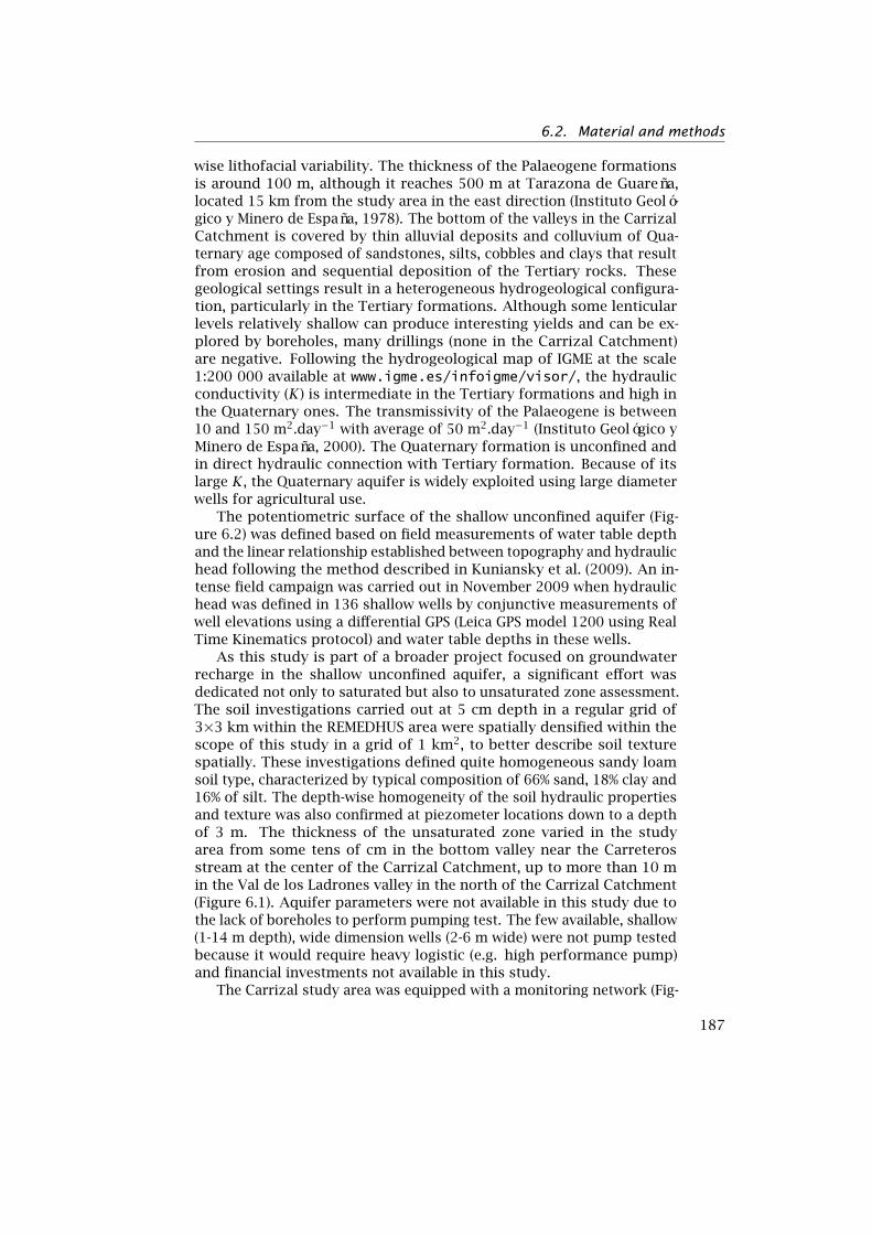
6.2. Material and methods
wise lithofacial variability. The thickness of the Palaeogene formationsis around 100 m, although it reaches 500 m at Tarazona de Guareña,located 15 km from the study area in the east direction (Instituto Geoló-gico y Minero de España, 1978). The bottom of the valleys in the CarrizalCatchment is covered by thin alluvial deposits and colluvium of Qua-ternary age composed of sandstones, silts, cobbles and clays that resultfrom erosion and sequential deposition of the Tertiary rocks. Thesegeological settings result in a heterogeneous hydrogeological configura-tion, particularly in the Tertiary formations. Although some lenticularlevels relatively shallow can produce interesting yields and can be ex-plored by boreholes, many drillings (none in the Carrizal Catchment)are negative. Following the hydrogeological map of IGME at the scale1:200 000 available at www.igme.es/infoigme/visor/, the hydraulicconductivity (K) is intermediate in the Tertiary formations and high inthe Quaternary ones. The transmissivity of the Palaeogene is between10 and 150 m2.day−1 with average of 50 m2.day−1 (Instituto Geológico yMinero de España, 2000). The Quaternary formation is unconfined andin direct hydraulic connection with Tertiary formation. Because of itslarge K, the Quaternary aquifer is widely exploited using large diameterwells for agricultural use.
The potentiometric surface of the shallow unconfined aquifer (Fig-ure 6.2) was defined based on field measurements of water table depthand the linear relationship established between topography and hydraulichead following the method described in Kuniansky et al. (2009). An in-tense field campaign was carried out in November 2009 when hydraulichead was defined in 136 shallow wells by conjunctive measurements ofwell elevations using a differential GPS (Leica GPS model 1200 using RealTime Kinematics protocol) and water table depths in these wells.
As this study is part of a broader project focused on groundwaterrecharge in the shallow unconfined aquifer, a significant effort wasdedicated not only to saturated but also to unsaturated zone assessment.The soil investigations carried out at 5 cm depth in a regular grid of3×3 km within the REMEDHUS area were spatially densified within thescope of this study in a grid of 1 km2, to better describe soil texturespatially. These investigations defined quite homogeneous sandy loamsoil type, characterized by typical composition of 66% sand, 18% clay and16% of silt. The depth-wise homogeneity of the soil hydraulic propertiesand texture was also confirmed at piezometer locations down to a depthof 3 m. The thickness of the unsaturated zone varied in the studyarea from some tens of cm in the bottom valley near the Carreterosstream at the center of the Carrizal Catchment, up to more than 10 min the Val de los Ladrones valley in the north of the Carrizal Catchment(Figure 6.1). Aquifer parameters were not available in this study due tothe lack of boreholes to perform pumping test. The few available, shallow(1-14 m depth), wide dimension wells (2-6 m wide) were not pump testedbecause it would require heavy logistic (e.g. high performance pump)and financial investments not available in this study.
The Carrizal study area was equipped with a monitoring network (Fig-
187
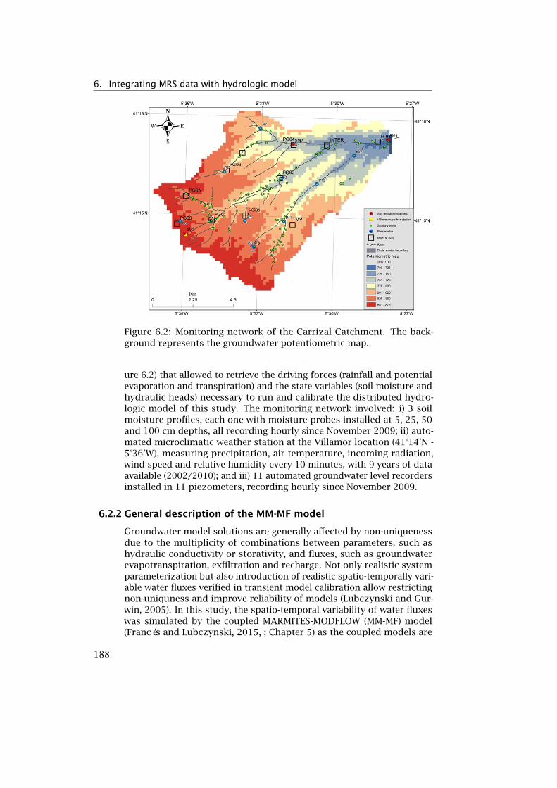
6. Integrating MRS data with hydrologic model
Figure 6.2: Monitoring network of the Carrizal Catchment. The back-ground represents the groundwater potentiometric map.
ure 6.2) that allowed to retrieve the driving forces (rainfall and potentialevaporation and transpiration) and the state variables (soil moisture andhydraulic heads) necessary to run and calibrate the distributed hydro-logic model of this study. The monitoring network involved: i) 3 soilmoisture profiles, each one with moisture probes installed at 5, 25, 50and 100 cm depths, all recording hourly since November 2009; ii) auto-mated microclimatic weather station at the Villamor location (41°14’N -5°36’W), measuring precipitation, air temperature, incoming radiation,wind speed and relative humidity every 10 minutes, with 9 years of dataavailable (2002/2010); and iii) 11 automated groundwater level recordersinstalled in 11 piezometers, recording hourly since November 2009.
6.2.2 General description of the MM-MF model
Groundwater model solutions are generally affected by non-uniquenessdue to the multiplicity of combinations between parameters, such ashydraulic conductivity or storativity, and fluxes, such as groundwaterevapotranspiration, exfiltration and recharge. Not only realistic systemparameterization but also introduction of realistic spatio-temporally vari-able water fluxes verified in transient model calibration allow restrictingnon-uniquness and improve reliability of models (Lubczynski and Gur-win, 2005). In this study, the spatio-temporal variability of water fluxeswas simulated by the coupled MARMITES-MODFLOW (MM-MF) model(Francés and Lubczynski, 2015, ; Chapter 5) as the coupled models are
188
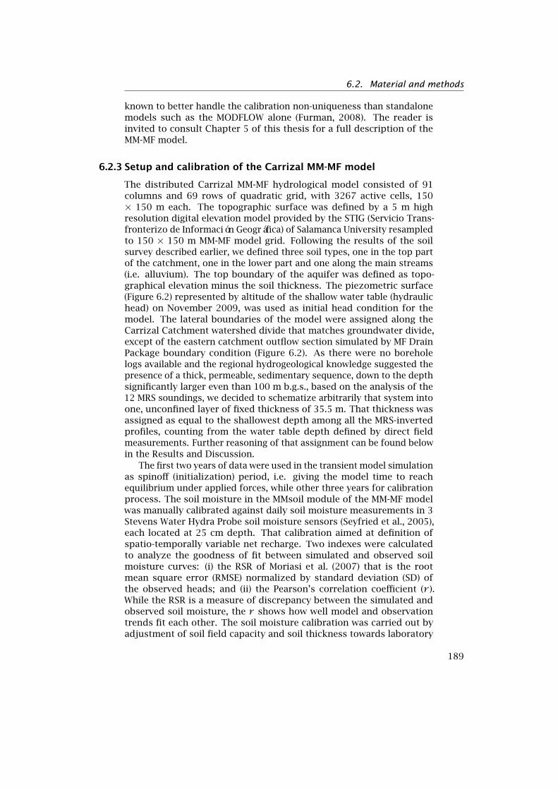
6.2. Material and methods
known to better handle the calibration non-uniqueness than standalonemodels such as the MODFLOW alone (Furman, 2008). The reader isinvited to consult Chapter 5 of this thesis for a full description of theMM-MF model.
6.2.3 Setup and calibration of the Carrizal MM-MF model
The distributed Carrizal MM-MF hydrological model consisted of 91columns and 69 rows of quadratic grid, with 3267 active cells, 150× 150 m each. The topographic surface was defined by a 5 m highresolution digital elevation model provided by the STIG (Servicio Trans-fronterizo de Información Geográfica) of Salamanca University resampledto 150 × 150 m MM-MF model grid. Following the results of the soilsurvey described earlier, we defined three soil types, one in the top partof the catchment, one in the lower part and one along the main streams(i.e. alluvium). The top boundary of the aquifer was defined as topo-graphical elevation minus the soil thickness. The piezometric surface(Figure 6.2) represented by altitude of the shallow water table (hydraulichead) on November 2009, was used as initial head condition for themodel. The lateral boundaries of the model were assigned along theCarrizal Catchment watershed divide that matches groundwater divide,except of the eastern catchment outflow section simulated by MF DrainPackage boundary condition (Figure 6.2). As there were no boreholelogs available and the regional hydrogeological knowledge suggested thepresence of a thick, permeable, sedimentary sequence, down to the depthsignificantly larger even than 100 m b.g.s., based on the analysis of the12 MRS soundings, we decided to schematize arbitrarily that system intoone, unconfined layer of fixed thickness of 35.5 m. That thickness wasassigned as equal to the shallowest depth among all the MRS-invertedprofiles, counting from the water table depth defined by direct fieldmeasurements. Further reasoning of that assignment can be found belowin the Results and Discussion.
The first two years of data were used in the transient model simulationas spinoff (initialization) period, i.e. giving the model time to reachequilibrium under applied forces, while other three years for calibrationprocess. The soil moisture in the MMsoil module of the MM-MF modelwas manually calibrated against daily soil moisture measurements in 3Stevens Water Hydra Probe soil moisture sensors (Seyfried et al., 2005),each located at 25 cm depth. That calibration aimed at definition ofspatio-temporally variable net recharge. Two indexes were calculatedto analyze the goodness of fit between simulated and observed soilmoisture curves: (i) the RSR of Moriasi et al. (2007) that is the rootmean square error (RMSE) normalized by standard deviation (SD) ofthe observed heads; and (ii) the Pearson’s correlation coefficient (r ).While the RSR is a measure of discrepancy between the simulated andobserved soil moisture, the r shows how well model and observationtrends fit each other. The soil moisture calibration was carried out byadjustment of soil field capacity and soil thickness towards laboratory
189

6. Integrating MRS data with hydrologic model
and field defined ranges, focusing on minimizing RSR and maximizingthe Pearson’s correlation coefficient (r ).
The groundwater MODFLOW module of the MM-MF model was calib-rated against time series of hydraulic head measurements in 11 piezo-meters. The water levels in piezometers were recorded by Keller (www.keller-druck.com) automated water table recorders. The head calibra-tion was done by adjustment of multipliers of MRS estimates of specificyield (Sy,MRS ) and MRS estimates of hydraulic conductivity (KMRS ). Inevery calibration run, one multiplier for the 12 Sy,MRS and anotherone for the 12 KMRS were assigned, which guaranteed the original pro-portionality between the MRS estimates of specific yield and hydraulicconductivity. The MODFLOW calibration of heads was carried out by trialand error adjustment of the two MRS multipliers focusing on minimizingRSR at the 11 monitored piezometers and maximizing the Pearson’scorrelation coefficient (r ). That calibration allowed finally, to select apair of MRS multipliers further used to estimate specific yield (Sy ) andhydraulic conductivity (K) at the 12 MRS survey locations as explainedbelow.
6.2.4 MRS contribution to hydrogeological parameterization
Distributed hydrological models, such as MM-MF, require definition ofhydrostratigraphic layers, aquifer parameters and water fluxes. Themain aim of the MRS measurements in this study was to characterizespatial variability of hydraulic parameters of the shallow unconfinedaquifer by integrating the MRS measurements in a coupled hydrologicalMM-MF model optimizing the MRS estimates of specific yield (Sy,MRS )and hydraulic conductivity (KMRS ).
6.2.4.1 Hydrogeophysical pre-MRS field measurements
Pre-MRS field measurements were carried out prior the MRS surveysassessing: i) natural magnetic field (B); ii) electromagnetic noise; andiii) geoelectrical subsurface profiles using Vertical Electrical Sounding(VES) or TDEM. The magnetic field and noise measurements were carriedout to confirm suitability of the selected site for the MRS survey and tooptimize that survey (Lubczynski and Roy, 2004) whereas the geoelec-trical profiles to support the MRS inversion process. The assessment ofnatural magnetic field was executed to determine the local scale magneticinhomogeneity and to determine Larmor frequency (fl) necessary forthe MRS survey. The magnetometric survey was carried out with twomagnetometers: G856 as rover and a G816 as a base in 12 selected MRSsurvey sites. In each selected MRS site, 36 magnetometric measurementswere carried out within 100 × 100 m quadratic or rhomboid area. Theelectromagnetic noise and the VES/TDEM measurements were performedin the pre-selected MRS-survey locations. The noise measurements weredone with a coil especially designed for the noise investigation (Plataet al., 2009). The VES investigations were executed with Syscal R2E res-
190

6.2. Material and methods
istivity meter from IRIS Instruments while the TDEM measurements witha 50 m square loop using a TEM-FAST 48 from Applied ElectromagneticResearch (AEMR).
6.2.4.2 MRS field measurements
The selection of the MRS sounding locations was a result of carefulGIS-based analysis of the land cover, available subsurface informationand pre-MRS field measurements. That selection attempted also tocover hydrological variability within the Carrizal Catchment and to haveshallow wells nearby, to provide direct information on the groundwatertable depth as auxiliary data in the MRS water detection process. As aresult 12 MRS locations were selected. In each site, the magnetic field(B) was measured directly before the MRS survey and the retrieved valuewas used to calculate the Larmor frequency required for the MRS survey.Since B varied with time, we also monitored its temporal variations duringthe MRS survey. The 12 selected MRS locations were surveyed in twofield campaigns, the first in April 2009 with 8 soundings (Uriarte Blancoet al., 2011) and the second in November 2009 with 4 soundings. Inboth campaigns, the NUMISLITE MRS equipment manufactured by IRISInstruments was used. The locations of the MRS sounding experimentsare presented in Figure 6.2. The 12 MRS surveys resulted in satisfactorydata coverage of 1 MRS survey per ∼6 km2, essential for appropriateconstrain of the distributed hydrological model. In 8 MRS surveys, a60 m square-shaped loop was used while in 4 sites, due to lower signal tonoise (S/N) ratio, a square-eight loop of 30 m side each, oriented parallelto adjacent electric power lines, was used with the aim to improve theS/N ratio. That configuration allowed to work in areas with relatively lowS/N ratio, where standard 60 m square-shape loop would not permit toperform MRS sounding correctly (Trushkin et al., 1994).
6.2.4.3 MRS data processing
For the inversion of the MRS sounding data, the new Samovar 11.3(Legchenko, 2011) was used. At each MRS survey location, the geoelec-trical profiles acquired through VES and/or TDEM were used in the calcu-lation of the Samovar "linear filter". The linear filter is a pre-calculationof the MRS response at the given location for a suite of theoretical layersat increasing depth levels, taking into account the MRS loop shape andsize, the range of excitation moment (Q), the subsurface geoelectricallayering in terms of resistivity and thickness, the Earth’s magnetic fieldmagnitude and its inclination.
The transient model of the unconfined Carrizal aquifer requiredpre-assignment of spatial variability of the specific yield. FollowingLubczynski and Roy (2003); Legchenko et al. (2004); Lubczynski andRoy (2005, 2007); Vouillamoz et al. (2012b), in medium to coarse grainmaterials such as the composition of the shallow Carrizal aquifer, the
191
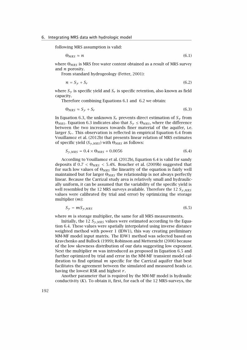
6. Integrating MRS data with hydrologic model
following MRS assumption is valid:
ΘMRS ≈ n (6.1)
where ΘMRS is MRS free water content obtained as a result of MRS surveyand n porosity.
From standard hydrogeology (Fetter, 2001):
n = Sy + Sr (6.2)
where Sy is specific yield and Sr is specific retention, also known as fieldcapacity.
Therefore combining Equations 6.1 and 6.2 we obtain:
ΘMRS ≈ Sy + Sr (6.3)
In Equation 6.3, the unknown Sr prevents direct estimation of Sy fromΘMRS . Equation 6.3 indicates also that Sy ≤ ΘMRS , where the differencebetween the two increases towards finer material of the aquifer, i.e.larger Sr . This observation is reflected in empirical Equation 6.4 fromVouillamoz et al. (2012b) that presents linear relation of MRS estimatesof specific yield (Sy,MRS ) with ΘMRS as follows:
Sy,MRS = 0.4×ΘMRS + 0.0056 (6.4)
According to Vouillamoz et al. (2012b), Equation 6.4 is valid for sandydeposits if 0.7 < ΘMRS < 5.4%. Boucher et al. (2009b) suggested thatfor such low values of ΘMRS the linearity of the equation is fairly wellmaintained but for larger ΘMRS the relationship is not always perfectlylinear. Because the Carrizal study area is relatively small and hydraulic-ally uniform, it can be assumed that the variability of the specific yield iswell resembled by the 12 MRS surveys available. Therefore the 12 Sy,MRSvalues were calibrated (by trial and error) by optimizing the storagemultiplier (m):
Sy =mSy,MRS (6.5)
where m is storage multiplier, the same for all MRS measurements.Initially, the 12 Sy,MRS values were estimated according to the Equa-
tion 6.4. These values were spatially interpolated using inverse distanceweighted method with power 1 (IDW1), this way creating preliminaryMM-MF model input matrix. The IDW1 method was selected based onKravchenko and Bullock (1999); Robinson and Metternicht (2006) becauseof the low skewness distribution of our data suggesting low exponent.Next the multiplier m was introduced as proposed in Equation 6.5 andfurther optimized by trial and error in the MM-MF transient model cal-ibration to find optimal m specific for the Carrizal aquifer that bestfacilitates the agreement between the simulated and measured heads i.e.having the lowest RSR and highest r .
Another parameter that is required by the MM-MF model is hydraulicconductivity (K). To obtain it, first, for each of the 12 MRS-surveys, the
192

6.3. Results and discussion
MRS estimates of aquifer transmissivity (TMRS ) were derived accordingto Equation 6.6 applying Samovar 11.3 inversion with its default CT0 =7× 10⁻⁹:
TMRS = CT0 ×∑ΘMRS(z)× (T1)2∆z (6.6)
where CT0 is Samovar 11.3 default MRS-transmissivity multiplier, ΘMRS(z)is MRS free water content at depth z, T1 is longitudinal relaxation timein milliseconds and ∆z is thickness of individual layer in meters.
In the next step, each transmissivity value was converted to hydraulicconductivity according to Equation 6.7:
KMRS = TMRS/ztot (6.7)
where KMRS is hydraulic conductivity derived by MRS and ztot =∑∆z is
total thickness of the aquifer in meters. The final aquifer transmissiv-ity and hydraulic conductivity are expressed by Equations 6.8 and 6.9respectively:
T = CT ×∑ΘMRS(z)× (T1)2∆z (6.8)
K= T/ztot (6.9)
After defining 12 TMRS values according to Equation 6.6 i.e. applyingCT0 = 7× 10⁻⁹, the 12 KMRS were calculated according to Equation 6.7and further interpolated using IDW1 method creating preliminary KMRSMM-MF model input matrix. Next the multiplier CT was introduced asin Equation 6.8 and 6.9 and further optimized in the MM-MF transientmodel calibration in order to find optimal CT value that facilitates bestthe agreement between the simulated and measured heads (lowest RSRand highest r ).
6.3 Results and discussion
An overview of the environmental conditions of the 12 MRS surveys char-acterizing their suitability for MRS soundings is presented in Table 6.1.The magnetic inhomogeneity (∆B) varied among the MRS-sites from 2 to12 nT (Table 6.1). Two of the twelve sites are presented in Figure 6.3 asexamples of the Carrizal Catchment magnetic field variability within theMRS loop scale. It can be observed that in the INTER 60×60 m squareloop (Figure 6.3a), the magnetic field was fairly constant (∆B = 6 nT),while in the PG05 with square-eight loop (Figure 6.3b), variability of themagnetic field was larger (∆B = 10 nT). In general the magnetic inhomo-geneity within the MRS survey sites of the Carrizal Catchment was lowas the largest ∆B in H-9 location (Table 6.1) did not exceed 12 nT, i.e.∆fl = 0.5 Hz on the Larmor frequency which can be considered nearlyhomogeneous field condition.
193
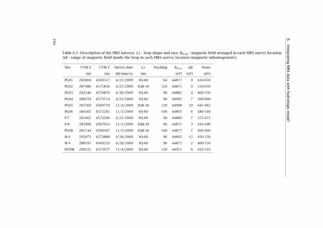
6.
Integ
rating
MR
Sdata
with
hyd
rolo
gic
model
Table 6.1: Description of the MRS surveys: Ls - loop shape and size; Bavg - magnetic field averaged in each MRS survey location;∆B - range of magnetic field inside the loop in each MRS survey location (magnetic inhomogeneity).
Site UTM X UTM Y Survey date Ls Stacking Bavg ∆B Noise
(m) (m) dd/mm/yy (m) (nT) (nT) (nV)
PG01 283669 4569517 4/21/2009 SQ-60 64 44877 9 450-650
PG02 287486 4571856 4/27/2009 SQ8-30 120 44875 9 550-650
PG03 282246 4570870 4/30/2009 SQ-60 96 44882 4 400-550
PG04 288259 4573714 4/23/2009 SQ-60 96 44905 7 500-600
PG05 285569 4569759 11/4/2009 SQ8-30 120 44908 10 445-465
PG06 284502 4572292 11/3/2009 SQ-60 100 44897 6 380-540
P-7 285402 4573260 4/21/2009 SQ-60 96 44889 7 375-475
P-8 285900 4567914 11/3/2009 SQ8-30 96 44871 3 410-490
PG08 281744 4569307 11/3/2009 SQ8-30 100 44877 7 300-400
H-9 292973 4573888 4/28/2009 SQ-60 96 44895 12 450-550
M-V 288197 4569233 4/28/2009 SQ-60 96 44875 2 400-550
INTER 290121 4573677 11/4/2009 SQ-60 120 44915 6 410-510
19
4
6.3. Results and discussion
The pre-MRS noise survey indicated low electromagnetic noise rangingfrom 375 to 650 nV (Table 6.1) suitable for MRS surveys in 11 out of the12 selected locations. The only one location where the noise was toohigh was discarded and replaced with a new, nearby location, H-9, withlower, comparable with other sites noise. In PG02, PG05, PG08 and P-8,due to the presence of adjacent electric power lines, a square-eight loopconfiguration parallel to the power line had to be used to reduce thenoise influence. During the MRS experiments the environmental noisedid not vary much, typically staying within 200 nV difference (Table 6.1);however, in the two cases, i.e. PG04 and P-7, the MRS measurements hadto be repeated because of temporally variable noise.
Figure 6.3: Magnetic field in MRS experiments: a) MRS-loop location withmedium magnetic field variability (INTER); b) MRS-loop location withhigher magnetic field variability (PG05).
The VES and TDEM results inverted into resistivity layers were usedas support of the MRS inversions. In order to characterize variability ofthe resistivity attributed to the modelled, shallow aquifer extent, for eachMRS survey location, the aquifer resistivity (Table 6.2) at each surveyedsite was estimated by weighted average of the resistivity layers within theaquifer thicknesses as defined by the MRS soundings. Except of the M-Vlocations with relatively large resistivity of 190 Ωm, in all other locations,the resistivities were low, in order of 10-30 Ωm.
The results of the 12 MRS surveys, inverted with Samovar 11.3 usingpreliminary standard CT0 = 7 × 10⁻⁹ and corresponding geoelectricalprofiles are presented in Table 6.2 and Figure 6.4 whereas the locationof the 12 MRS surveys can be found in Figure 6.2. In order to enhancereadability of the MRS survey results, all the MRS profiles were presentedwithin the same depth range, water content and decay time scale. Due tothe excitation limit of the NUMISLITE MRS equipment and the loop size upto Ls = 60 m, the Samovar inversions of the MRS surveys allowed for themaximum investigation depth < 90 m b.g.s., which for the four surveyswith square-eight loop (PG02, PG05, PG08 and P-8) was still significantlylower.
195

6. Integrating MRS data with hydrologic model
Figure 6.4: Scaled MRS inversion results of ΘMRS and T1 with preliminary,standard, CT0 = 7×10⁻⁹. Black lines show the assigned in the hydrologicmodel top and bottom aquifer boundaries. On the right side of eachimage, resistivity profiles in logarithmic scale are shown by blue line forVES and brown line for TDEM method.
196

6.3
.R
esults
and
discu
ssion
Table 6.2: MRS survey results: GWTD - groundwater table depth; Daq - thickness of the aquifer; ρ - resistivity of the aquifer;ΘMRS - MRS water content of the aquifer; T1 - decay time constant; Sy,MRS - MRS estimate of specific yield; KMRS , TMRS - MRSestimate of hydraulic conductivity and aquifer transmissivity based on standard multiplier CT0 = 7× 10⁻⁹; Sy - calibratedspecific yield; K - calibrated hydraulic conductivity using optimized MRS transmissivity multiplier CT .
Site Altitude GWTD Daq ρ ΘMRS T1 Sy,MRS TMRS KMRS Sy K
(m.a.s.l.) (m) (m) (Ωm) (%) (ms) (%) (m2.d−1) (m.d−1) (%) (m.d−1)
PG01 850 1.9 >57 30 6.1 390 2.4 246 6.9 2.4 3.4
PG02 792 2.8 >37 10 10.8 400 4.3 357 10.1 4.3 5.0
PG03 872 7.7 >58 22 5.3 262 2.2 95 2.7 2.2 1.3
PG04 777 10.5 35.5 13 4.6 274 1.8 83 2.3 1.8 1.1
PG05 846 9.1 >44 11 4.4 229 1.8 49 1.4 1.8 0.7
PG06 825 6.5 >76 13 5.5 124 2.2 23 0.6 2.2 0.3
P-7 810 6.2 >69 16 5.9 415 2.4 213 6.0 2.4 3.0
P-8 853 2.0 >44 15 5.2 440 2.1 218 6.2 2.1 3.1
PG08 877 5.4 >42 17 3.9 409 1.6 134 3.8 1.6 1.6
M-V 835 4.0 >53 190 3.2 296 1.3 65 1.8 1.3 0.9
INTER 763 6.5 >70 15 7.9 245 3.2 102 2.9 3.2 1.4
H-9 751 3.0 45 15 4.7 302 1.9 84 2.4 1.9 1.2
Mean 6.3 31 5.6 315 2.3 137 3.4 2.3 1.9
St.Dev 2.8 31 2.0 96 0.8 97 2.8 0.8 1.4
19
7
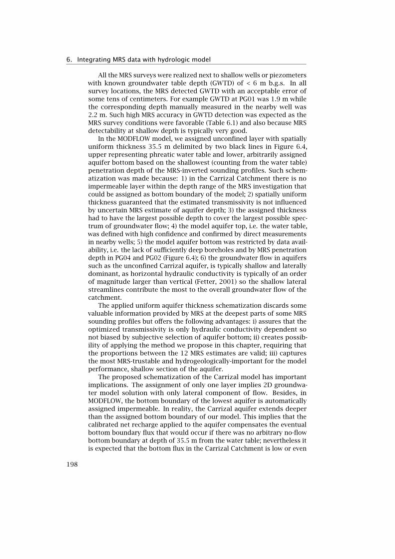
6. Integrating MRS data with hydrologic model
All the MRS surveys were realized next to shallow wells or piezometerswith known groundwater table depth (GWTD) of < 6 m b.g.s. In allsurvey locations, the MRS detected GWTD with an acceptable error ofsome tens of centimeters. For example GWTD at PG01 was 1.9 m whilethe corresponding depth manually measured in the nearby well was2.2 m. Such high MRS accuracy in GWTD detection was expected as theMRS survey conditions were favorable (Table 6.1) and also because MRSdetectability at shallow depth is typically very good.
In the MODFLOW model, we assigned unconfined layer with spatiallyuniform thickness 35.5 m delimited by two black lines in Figure 6.4,upper representing phreatic water table and lower, arbitrarily assignedaquifer bottom based on the shallowest (counting from the water table)penetration depth of the MRS-inverted sounding profiles. Such schem-atization was made because: 1) in the Carrizal Catchment there is noimpermeable layer within the depth range of the MRS investigation thatcould be assigned as bottom boundary of the model; 2) spatially uniformthickness guaranteed that the estimated transmissivity is not influencedby uncertain MRS estimate of aquifer depth; 3) the assigned thicknesshad to have the largest possible depth to cover the largest possible spec-trum of groundwater flow; 4) the model aquifer top, i.e. the water table,was defined with high confidence and confirmed by direct measurementsin nearby wells; 5) the model aquifer bottom was restricted by data avail-ability, i.e. the lack of sufficiently deep boreholes and by MRS penetrationdepth in PG04 and PG02 (Figure 6.4); 6) the groundwater flow in aquiferssuch as the unconfined Carrizal aquifer, is typically shallow and laterallydominant, as horizontal hydraulic conductivity is typically of an orderof magnitude larger than vertical (Fetter, 2001) so the shallow lateralstreamlines contribute the most to the overall groundwater flow of thecatchment.
The applied uniform aquifer thickness schematization discards somevaluable information provided by MRS at the deepest parts of some MRSsounding profiles but offers the following advantages: i) assures that theoptimized transmissivity is only hydraulic conductivity dependent sonot biased by subjective selection of aquifer bottom; ii) creates possib-ility of applying the method we propose in this chapter, requiring thatthe proportions between the 12 MRS estimates are valid; iii) capturesthe most MRS-trustable and hydrogeologically-important for the modelperformance, shallow section of the aquifer.
The proposed schematization of the Carrizal model has importantimplications. The assignment of only one layer implies 2D groundwa-ter model solution with only lateral component of flow. Besides, inMODFLOW, the bottom boundary of the lowest aquifer is automaticallyassigned impermeable. In reality, the Carrizal aquifer extends deeperthan the assigned bottom boundary of our model. This implies that thecalibrated net recharge applied to the aquifer compensates the eventualbottom boundary flux that would occur if there was no arbitrary no-flowbottom boundary at depth of 35.5 m from the water table; nevertheless itis expected that the bottom flux in the Carrizal Catchment is low or even
198

6.3. Results and discussion
negligible as the shallow aquifer has quite large horizontal hydraulicconductivity in order of 10 m.d−1, favoring shallow-lateral flow withshort residence time (Fetter, 2001).
The MMsoil model calibration of soil moisture provided good matchbetween measured and simulated soil moisture, and as a result generatedspatio-temporally variable net recharge that was further used as input inMODFLOW calibration. An example of soil moisture calibration for theselected time series SM1 sensor measurements is presented in Figure 6.5.That calibration shows good agreement between simulated and measuredsoil moisture records and was characterized with r= 0.87 and RSR=0.51.The head calibration in MODFLOW was completed after 49 runs, eachtime with a different values of m and CT , although not all the runs werestable. The unstable runs are marked in white in the two left panels inFigure 6.5. The best, optimized model solution based on three years ofhead calibration with the lowest RSR = 4.28 and the highest r = 0.74, wasobtained for m=1 and CT = 3.5× 10⁻⁹. The Sy,MRS is best defined usingr while the KMRS using RSR. This is because Sy,MRS variations influencethe amplitude of the piezometric curve, thus the trend and the fittingbetween simulated and observed curve to which r is sensitive, while KMRSvariations modify the distance (offset) between the two curves, which isreflected in the RSR value . An example of modeled and observed head inone piezometer P1 with well-retrieved pattern of temporal variability ofwater table fluctuation is shown in Figure 6.5. The shift between modeledand observed heads is a consequence of model scale: the Carrizal modelis setup with a resolution of 150×150 m, so the P1 head observationhas likely a shift due to the topographically constrained head variabilitywithin the grid cell. Nevertheless, the most important in transient modelcalibration temporal pattern of head measurements (Lubczynski andGurwin, 2005) was well retrieved.
The Sy,MRS input parameter of the MM-MF model estimated usingEquation 6.4 (Vouillamoz et al., 2012b) is listed in Table 6.2 and presentedspatially in Figure 6.6. We used Equation 6.4 to estimate Sy,MRS eventhough our average ΘMRS was 5.6%, i.e. slightly above the range adoptedby Vouillamoz et al. (2012b). The estimated Sy,MRS varied from 1.3%in PG04 to 4.3% in PG02, with a mean of 2.3% and standard deviationσ = 0.8%. It is remarkable that through the model calibration, them multiplier was not changed (m = 1) so that Sy,MRS did not needany adjustment in the process of transient model calibration, implyingSy,MRS ≈ Sy according to Equation 6.5. The difference between Sy andSy,MRS was within the resolution of calibration process, which shows thatthe MRS estimate of specific yield (Sy,MRS ) computed using Equation 6.4provided a good guess of Sy in the Carrizal Catchment. Figure 6.6 showsspatial distribution of Sy in the Carrizal Catchment that ranged from 1%to 4.5%, pointing at significant aquifer homogeneity.
The KMRS input parameter of the MM-MF model estimated usingEquations 6.6 and 6.7 is listed in Table 6.2. The KMRS varied from0.6 m.d−1 in PG06 to 10.1 m.d−1 in PG02 with a mean of 3.9 m.d−1 andstandard deviation σ= 2.8 m.d−1. The optimized in the calibration of
199

6. Integrating MRS data with hydrologic model
Figure 6.5: Calibration analysis. The two panels at the left show RSR(upper panel) and r (lower panel) computed in relation to simulated andobserved hydraulic heads and varying the multipliers of MRS estimatesof specific yield (Sy,MRS ) and hydraulic conductivity (KMRS ); in whitecombination of parameters that do not provide a stable solution in MM-MF model, in dark blue best solution. The two panels at the right presentexamples of model calibration of soil moisture at SM1 location (upperpart) and hydraulic head at PG1 (lower part).
groundwater model CT = 3.5×10⁻⁹ is specific for the Carrizal Catchment.Considering that initially used in the calibration CT0 = 7 × 10⁻⁹, theoptimized in MM-MF K was only twice lower than KMRS (Table 6.2). Theoptimized K varied from 0.3 m.d−1 in PG06 to 5.0 m.d−1 in PG02 witha mean of 1.9 m.d−1 and standard deviation σ=1.4 m.d−1. Consideringthat hydraulic conductivity is spatially log-normally distributed (Fetter,2001), the spatial variability of the Carrizal Catchment K presented inFigure 6.7 can be considered as very low pointing at significant aquiferhomogeneity.
Despite low spatial variability of Sy and K, there was still some in-ternal variability in the estimates of Sy,MRS and KMRS , although notlarge. The maximum differences within Sy,MRS and KMRS were observedbetween PG02 and PG05 locations (Table 6.2). We analyzed the granulo-metry of the soil samples from 3 m depth in these two locations to seeif what was depicted by MRS ΘMRS and T1 did indeed properly reflectfield lithological and hydrogeological differences. We found that the soilmaterial in the PG02 contained 79% of sand and was coarser than in thePG05 that contained 56% of sand. This was in line with the MRS estimatesof Sy,MRS and KMRS and confirmed that MRS was well able to depict the
200
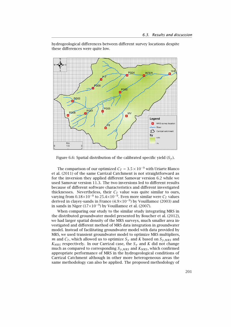
6.3. Results and discussion
hydrogeological differences between different survey locations despitethese differences were quite low.
Figure 6.6: Spatial distribution of the calibrated specific yield (Sy ).
The comparison of our optimized CT = 3.5×10⁻⁹ with Uriarte Blancoet al. (2011) of the same Carrizal Catchment is not straightforward asfor the inversion they applied different Samovar version 6.2 while weused Samovar version 11.3. The two inversions led to different resultsbecause of different software characteristics and different investigatedthicknesses. Nevertheless, their CT value was quite similar to ours,varying from 0.18×10⁻⁹ to 25.4×10⁻⁹. Even more similar were CT valuesderived in clayey-sands in France (4.9×10⁻⁹) by Vouillamoz (2003) andin sands in Niger (17×10−9) by Vouillamoz et al. (2007).
When comparing our study to the similar study integrating MRS inthe distributed groundwater model presented by Boucher et al. (2012),we had larger spatial density of the MRS surveys, much smaller area in-vestigated and different method of MRS data integration in groundwatermodel. Instead of facilitating groundwater model with data provided byMRS, we used transient groundwater model to optimize MRS multipliers,m and CT , which allowed us to optimize Sy and K based on Sy,MRS andKMRS respectively. In our Carrizal case, the Sy and K did not changemuch as compared to corresponding Sy,MRS and KMRS , which confirmedappropriate performance of MRS in the hydrogeological conditions ofCarrizal Catchment although in other more heterogeneous areas thesame methodology can also be applied. The proposed methodology of
201

6. Integrating MRS data with hydrologic model
Figure 6.7: Spatial distribution of the calibrated hydraulic conductivity(K).
aquifer parameterization based on optimizing m and CT multipliers indistributed hydrological models represents an alternative to the methodof cross referencing MRS surveys with pumping test data. As the othermethod that uses pumping test data implicitly, our method also offersan opportunity of definingm and CT multipliers which are characteristicfor the investigated area so in case of follow up MRS surveys in thatarea (or adjacent, hydrologically similar areas), these multipliers can beused for direct estimation of aquifer Sy , T and K. The proposed methoddoes not need pumping test data, but requires a good quality inputdata, preferably long time series data, allowing for a tight constrain ofa calibrated, distributed and preferably coupled, transient hydrologicalmodel, although solution applying standard, standalone groundwatermodel would also suffice.
When calibrating steady-state model, only CT multiplier can be de-rived. Bothm and CT multipliers can be derived in transient models. Themost effective hydrological model constrain and therefore the highestreliability can be achieved in transient and coupled models such asthe presented Carrizal model - in transient, because calibration againsttemporal data optimally reduces hydrological model non-uniqueness(Lubczynski, 2011) and in coupled, because such models handle theaquifer input fluxes in more reliable manner than stand alone models(Furman, 2008; Francés and Lubczynski, 2015, ; Chapter 5). If in an
202

6.4. Conclusions
investigated area pumping tests are available, then certainly they shouldbe used as model input, because they enhance reliability of models.However, if not available, then the proposed optimization method is anopportunity that should be considered if appropriate data to setup amodel is available. The important question related to the applied op-timization method, but also to the common practice of calibrating MRSresults with pumping test data is, when and under which conditions inan investigated area, only one storage (m) and only one transmissivitymultiplier (CT ) representative for that investigated area can be applied.We hypothesize that m and CT depend on the hydraulic model of waterflow at the pore scale of the analyzed aquifers. In that respect thereare 4 main types of such hydraulic models: primary porosity (e.g. un-consolidated sand), secondary porosity (e.g. fractured granite), doubleporosity (e.g. sandstone) and karst (e.g. limestone). If in an investigatedstudy area, there are rocks of different hydraulic models, then certainlydifferent m and different CT have to be introduced. However, whetherwithin investigated rock types of the same hydraulic model but differingfor example by texture or lithology, only one m and one CT can be used,this requires further testing and cross-referencing with pumping teststhat unfortunately were not available in this study.
6.4 Conclusions
The MRS technique is highly suitable for its integration with distributed,hydrological models because: i) it provides quantitative estimates ofstorage and flow parameters (Sy , T , K) at the survey location; ii) thevolumes investigated by MRS survey can be easily adjusted in a distrib-uted hydrological model by grid and layering adjustment so that the twoare comparable in scales.
We proposed a novel method of integrating MRS results in a distrib-uted, coupled transient hydrological model using Carrizal Catchmentstudy area as an example. In that method we assumed that individualMRS sounding results can be biased but the relative differences betweenMRS survey results at different locations of the catchment reflect realhydrological differences between these locations. Following that assump-tion, we assigned specific yield and transmissivity multipliers (m andCT respectively) to the corresponding MRS-specific yield and MRS trans-missivity estimates and optimized the two multipliers in the transient,coupled hydrological model calibration.
The MRS integration with hydrological model of the Carrizal Catch-ment area allowed to: i) calibrate that model; ii) derive m=1 and CT =3.5× 10⁻⁹ that can be used in future MRS investigations in the CarrizalCatchment (and/or adjacent areas with similar hydrogeological condi-tions) to convert MRS survey results into hydrogeological output; iii)acquire spatial variability of specific yield and transmissivity/hydraulicconductivity data in the Carrizal Catchment that showed to be pretty low
203

6. Integrating MRS data with hydrologic model
pointing at significant aquifer homogeneity; iv) present and explain theproposed, novel method of MRS data integration in hydrological model.
The values of MRS estimates of Sy,MRS , TMRS and KMRS defined inthe Carrizal Catchment were close to the corresponding, finally optim-ized values of specific yield (Sy ) and hydraulic conductivities (K); thisconfirmed functional capability of MRS in quantitative aquifer paramet-erization.
If pumping tests are available, then they should be used to define MRSmultipliers of the hydrogeological parameters; however if not available,but there is enough data to setup coupled, distributed hydrologicalmodel or at least standalone groundwater model, then the proposed inthis study MRS integration method provides a valuable alternative thatshould be further tested in various hydrogeological conditions againstpumping test data.
204

7Conclusions
The performance of coupled hydrological models is dependent on qualityand amount of data available. In this study, various non-invasive hydro-geophysical methods were tested regarding subsurface parametrizationand their potential contribution to the design of conceptual models. Thehydrogeophysical applications were optimal when integrated with remotesensing and standard field invasive methods of data acquisition, used forinterpolation or extrapolation and calibration. In particular, remote sens-ing was crucial to detect and map the main hydrogeological features atthe catchment scale (Chapters 2 and 4). The geoelectrical method allowedto depict the hydrostratigraphy of the hard rocks (Chapter 4) and coastalaquifers (Chapter 3) . Performed at key sites, they highlighted importantcharacteristics for the understanding of aquifer hydrodynamic relation-ships between hydrostratigraphical units. The geoelectrical methodcan be complemented by 1D time domain (TDEM) and 2D frequencydomain (FDEM) electromagnetic methods that are faster to implementin the field, although more sensitive to ambient electromagnetic noiseinduced for example by human activities and sea dynamic. For shallowsubsurface investigation, the 2D FDEM method retrieved efficiently thespatial variation of subsurface electrical conductivity related with claycontent in the Pisões study case (Chapter 2) and freshwater-saltwaterinterface in the coastal aquifer case (Chapter 3). The multi-frequency2D FDEM method, combined with the laterally constrained inversiontechnique, applied in the hard rock study case of Sardón (Chapter 4),showed to be very efficient, providing long cross-sections depicting largehydrogeological structures. The MRS technique was the only geophysicalmethod that could provide quantitative assessment of subsurface. TheMRS signal processing allows to determine storage and flow parameters,such as specific yield and hydraulic conductivity, although in new assess-ment areas, these parameters require calibration which typically is doneby pumping tests. In contrast, in the sedimentary aquifer of the Car-rizal catchment (Chapter 6), such calibration was carried out within theMARMITES-MODFLOW model. The magnetic resonance sounding (MRS)technique proved to be particularly suitable for integration with distrib-uted, hydrological models because it provides quantitative estimatesof storage and flow parameters at the scale of the hydrological model.In hard rocks, as in the Sardón area (Chapter 4), not every sounding
205

7. Conclusions
provided valid signal due to low quantities of subsurface water involvedand high clay content. Particularly difficult was data acquisition overthe fresh fractured rocks where low quantities of water were attributedto secondary porosity only, but surveys carried out over saprolite weremore successful.
The joint use of different but complementary hydrogeophysical meth-ods, adapted to different hydrogeological settings, showed to be highlybeneficial in the presented study cases, thus future research will follow inthat direction. For instance, the joint use of FDEM/TDEM and MRS, sincethey target at different, complementary subsurface properties, namelyelectrical conductivity and water content, showed to be very efficient,particularly in coastal areas where MRS retrieves the quantitative char-acteristics of the water bearing subsurface layers while TDEM retrievesthe qualitative (salinity) characteristics. However, as the ambient elec-tromagnetic noise is particularly high in urbanized coastal areas, itsfiltering should be improved for both methods. Ground-based electricand electromagnetic methods present low mobilization cost and highspatial resolution so are suitable for rather small areas. Due to thesecharacteristics, they can also beneficially complement, at the local scale,airborne electromagnetic surveys that are nowadays frequently appliedfor hydrogeological studies at regional or national scale. Related with thecomplementarity of the hydrogeophysical methods, the MRS techniquehas its particular importance to complement the airborne electromag-netic surveys because of its unique capability to retrieve quantitativeinformation regarding aquifer parameters. In hard rocks, the successof MRS survey is still limited but could be improved by optimizing: (i)the MRS loops and the instrumentation (larger pulse moment, betternoise rejection capability and shorter dead-time); (ii) the retrieval of thestorage parameters, namely the separation of gravitational water fromcapillary water based on MRS measurements. The latter issue showed re-cently a progress with the introduction of the concept of apparent cutofftime, which relates the MRS decay time with the aquifer storage property(Vouillamoz et al., 2012b, 2014a,b). In parallel, laboratory studies werealso performed to establish better relationships between aquifer andMRS parameters (Stingaciu et al., 2010; Boucher et al., 2011; Costabel andYaramanci, 2011, 2013), showing that MRS capacity can also be extendedto the investigation of water percolation and storage in the vadose zone.Moreover, in hard rock aquifers and other heterogeneous geological me-dium, the new 3D MRS data acquisition and inversion (Legchenko et al.,2011; Chevalier et al., 2014) can make possible to retrieve the aquiferstructures at the local scale, which may be of great help in solving criticalissues for water supply and borehole sitting, as well as for understandingthe hydraulic functioning of structurally complex aquifers. All these pro-gresses confirm that the MRS technique can be used as a tool to routinelyparameterize aquifers at lower cost than by drilling and pumping tests.
The coupled hydrological modeling approach is sophisticated anddata demanding technique but, in return, provides a detailed assessmentof surface and subsurface water fluxes and a better understanding of
206

complex dynamics of hydrological systems than by applying standard,standalone groundwater models. This study proposes a novel hydro-logical conceptualization of coupled models of surface, unsaturatedand saturated zones, involving numerical implementation of subsurfaceevapotranspiration built in the newly developed MARMITES code coupledwith MODFLOW-NWT model (Chapter 5). The novelty of that conceptu-alization involves partitioning and sourcing of subsurface evapotran-spiration, in which transpiration, in contrast to evaporation, is watertable depth independent and driven mainly by the climatic conditions,while contributions of water sources (saturated or unsaturated zone) aredependent on water potential schematized by set of lumped parameters.The appropriate performance of MARMITES-MODFLOW was confirmedon the La Mata hard rock study case (Chapter 5) and validated against in-dependent studies (van der Tol, 2012; Balugani et al., 2015; Reyes-Acosta,2015) and states variables measured in the field (soil moisture and hy-draulic heads). The capability of MARMITES-MODFLOW in integratingMRS method in the model calibration was also tested in the Carrizalsedimentary rock study case. The model-based optimization of the MRS-estimates of aquifer hydraulic parameters turned to be very promisingand created alternative to expensive pumping test parameterization.
As an open source code, the MARMITES model can be easily improvedand modified. In future, it would be relevant to implement the followingfeatures: (i) currently, the transpiration assessment is lumped at the gridcell; it could be optionally attributed to each vegetation species in orderto assess their individual impacts on water resources; (ii) the routing ofsurface water and the re-infiltration of produced runoff should be im-plemented in order to separate better surface runoff from groundwaterrunoff and introduce them as variables in the calibration process; (iii)more studies are required to define the vegetation parameters of thegroundwater transpiration defined in Chapter 5; seasonal monitoring ofsap flow, soil moisture, water potential and groundwater level at treeslocated in various topographical positions, such as drainage area andtop of hill, may provide important information to calibrate the paramet-ers of the novel groundwater transpiration function. In this study theapplication of remote sensing was limited to the extrapolation of theinvestigated property and to the mapping of terrain characteristics. How-ever, remote sensing can also be used for quantitative, spatio-temporalassessment of soil moisture (Jackson et al., 1996; Houser et al., 1998)and evapotranspiration (Su, 2002) that can be directly integrated as inputin the MARMITES model to constrain the calibration process.
Sensitivity analysis and uncertainties assessment related with thewater fluxes and water balance retrieved by the coupled MARMITES-MODFLOW model are still to be implemented. Automatic parameteroptimization algorithm such as singular value decomposition and Tik-honov regularization, for instance applied in PEST (Doherty, 2015), andhybrid genetic algorithms (Basokur et al., 2007; Yao and Guo, 2014)should be applied in the MARMITES-MODFLOW calibration of catchmentscale models. However, the practical implementation of such algorithms
207

7. Conclusions
in standard personal computers is currently hardly feasible, as the op-timization methods require many model runs and the running time ofcomplex coupled models is very long. Alternative solutions based onparallel computing implemented on clusters of individual computers oron cloud computing using virtual machines are being developed (Huntet al., 2010; Muffels et al., 2012; Welter et al., 2012; Fienen and Hunt,2015), allowing this way to reduce drastically the total time of parameteroptimization. It is expected that these solutions will allow in few yearsto compute routinely the crucial sensitivity analysis and uncertaintiesassessment of complex hydrological models.
208

AUsing Ground Penetrating Radarto investigate the groundwatertable depth in weathered granites- Sardón case study, Spain
A.1 Introduction
Groundwater modeling is nowadays recognized as the best tool to sup-port management of groundwater resources (?). Presently, informationon the depth and movement of groundwater is collected from a lim-ited number of often widely spaced, piezometers and observation wells(Bentley and Trenholm, 2002; Doolittle et al., 2006) to prepare the poten-tiometric map which can be used to estimate groundwater flow direction,flow velocities, and the location of discharge and recharge areas (Livariand Doolittle, 1994). These methods of data acquisition provide in-formation in specific, drilled boreholes where access to groundwater isrelatively easy. In that respect, ground penetrating radar (GPR) offerspromising perspectives for high resolution, continuous and large scalecharacterization and monitoring of hydrological systems.
GPR has been primarily used to image the subsurface and detect bur-ied objects (Annan, 2002; Lambot et al., 2008; Slob et al., 2010) by radiat-ing electromagnetic waves into the ground and recording the reflectionsfrom boundaries of subsurface material having different electromagneticparameters. Because of rapid rates of signal attenuation, the penetrationdepth of GPR is greatly reduced in soils that have high electrical conduct-ivity (Doolittle et al., 2007). The amount of electromagnetic energy that is
This chapter is based on: Using ground penetrating radar to investigate the watertable depth in weathered granites - Sardón case study, Spain. Mahmoudzadeh, M., A.Francés, M. Lubczynski, and S. Lambot (2012), Journal of Applied Geophysics, 79, 17-26.The author of this thesis participated or realized the following tasks: (i) acquisition,processing and interpretation of the ERT data; (ii) acquisition of the GPR and associatedDGPS data; (iii) definition of the general methodology, which mainly consisted to interpretthe field GPR data by comparing them with GPR forward models.
209

A. Appendix - Using GPR to investigate the groundwater table depth
reflected by an interface is dependent upon the electromagnetic contrastbetween the two media. The reflection coefficient of the subsurfacerepresents the ratio between the reflected and incident fields. Abruptboundaries that separate contrasting materials reflect more energy thangradual boundaries that separate layers with similar electrical properties(Lambot et al., 2004; Bano, 2006).
The dielectric constant of soil materials is principally dependent uponsoil moisture but also varies to some extent with temperature, density,and frequency. In low conductive materials, the soil moisture is themajor contributor to the soil dielectric constant (Bentley and Trenholm,2002; Topp et al., 1980). Nakashima et al. (2001) showed that when thereis water in a medium, like a groundwater layer, whose dielectric constantis quite different from the non-saturated media, it is possible to identifythe medium within a multitude of ambiguous media. In coarse-texturedsoils, the capillary fringe is narrow (Doolittle et al., 2006) which typicallyleads to a strong radar reflection. While on the contrary, in fine-texturedsoil materials, the height of the capillary fringe is larger than in coarse-texture materials with a smooth transition between the dry and saturatedsoils. Bentley and Trenholm (2002) showed that GPR can measure thetop of the capillary fringe and obtained an accuracy of ∼20 cm underfavorable conditions. They also investigated most of the error sourceson the estimation of the groundwater table depth (GWTD) and foundthat the main sources of uncertainty are due to GPR velocity estimatesand predicting the height above the groundwater table of the capillaryfringe reflection.
Our objectives in this research are: (1) to find the spatial distributionof the groundwater table depth in the granitic Sardón catchment (Spain)with the continuous coverage along a transect, (2) to investigate the abilityof GPR to detect the reflection from the underlying fissured granite orbedrock and (3) to validate the GPR data using different geophysicaltechniques. In that respect, we used a pulse radar to collect the GPRdata along 37 transects, with some of them crossing perpendicularlythe streams of the Sardón river which was dry during the survey period.GPR simulations based on the stratigraphy of the Sardón subsurfacewere performed using GprMax2D (Giannopoulos, 2005) to provide someinsights for better interpreting the radar images. Electrical resistivitytomography (ERT) was used along several GPR transects at the sameperiod to investigate the groundwater table and the bedrocks. Soilsampling in the shallow surface was performed throughout the studyarea at the same period to give us information regarding the soil physicalproperties. The water level depth of the existent wells was used to verifythe GPR results and calibrate the time-depth relation in the relevant GPRprofiles. In order to estimate the shallow soil electrical properties, weused frequency domain reflectometry (FDR) for the profiles when theexact WTD information from the observation wells was not available.
210

A.2. Materials and Methods
A.2 Materials and Methods
A.2.1 The study area
The Sardón catchment study site is located in the central-western part ofIberian Peninsula in Spain (Fig. A.1). The size of the catchment is ∼80km2 characterized by well defined boundaries. It has low human impactbecause of low human population. The study area has a fault line alongthe main stream of Sardon river and typical fractured granite rocks withstandard hard rock hydrology (?).
The climate in Sardón is semi-arid and it is typical for the centralpart of the Iberian Peninsula. The 23-year mean rainfall, estimated onthe base of 6 Spanish Meteorological Institute rain gauges located in thesurroundings of the study area was ∼500 mm.year−1. The warmest andthe most dry months in this catchment are July and August when theaverage temperature is ∼22rC and rainfall is less than 20 mm.month−1
(?). Sardón river is dry from mid-June to mid-October and in the rest ofthe year performs a role of a drain, specially for direct runoff. The landcover in Sardón is characterized by natural woody-shrub vegetation.
Granite compositions of the rocks influence on the geology and hydro-geology in the study area. The hydrology of Sardón is strongly influencedby weathering and fracturing process. We can generally recognize threehydrogeological layers in Sardón catchment. The top layer which is notconsolidated because of the weathered and alluvial deposits, has a thick-ness on average 0-5 m up to 10 m (?). The soil texture of this layer iscoarse which includes 52-90% sand, 7-26% silt, and 4-22% clay obtainedby soil sampling. Calculating the transition zone and capillary fringe forthis type of soil led to ∼10 cm thickness which is negligible compared toour used GPR signal wavelength. The second layer is fractured granitewith intercalations of granodiorites, schists, gneises and quartzites thatstraggly outcrops in the study area (?). The thickness of this layer variesbetween ∼60 m in the central part of the catchment to a few metersin the upland areas (?). Last layer is massive granite with some gneissinclusions that has formed impermeable rock basement. This layer isdeepest in the center of catchment and near the Sardón boundaries isshallowest and can outcrop locally (Fig. A.2). The groundwater table astypical for granitic areas is shallow and mostly occurs in unconsolidatedrocks.
A.2.2 Data acquisition
We used a time-domain GPR system (model SIR-20, Geophysical SurveySystems, Inc., GSSI, Salem, Massachusetts, USA) combined with a trans-mitting and receiving 200 MHz shielded bowtie antenna as an impulseradar and a survey wheel for positioning. The used configuration type forour survey provided 512 samples/scan and each sample included 16 bitsto record. GPR produces a Ricker-type pulse with frequency bandwidthof 50-600 MHz. Gain functions were applied to highlight subsurface
211

A. Appendix - Using GPR to investigate the groundwater table depth
E1
E7
E4
E5
E6
E3E2
E8
P5
P7
P6
P8
P3
P4
P2
P1
R5R4
R3
R2
R1
W2W3
W1
W6
W5
W4
W8
W9
W7
W11
W10
731000 732000 733000 734000 735000 736000 737000 738000 739000 740000 741000 742000 743000
4548
000
4550
000
4552
000
4554
000
4556
000
4558
000
LEGEND:ERT Profile
Well (Piezometer)
Explained GPR Transects in the paper
Pond
Sardon catchment boundary
Sardon Streams
Other GPR transects
Elevation (m)715 - 740
741 - 765
766 - 790
791 - 815
816 - 840
841 - 865
Andalucia
AragonCastilla y Leon
Galicia
Castilla-La Mancha
Cataluna
Extremadura
Asturias
Valenciana
Murcia
Navarra
Madrid
Pais Vasco
La Rioja
Cantabria
Isles Baleares
Isles Baleares
Spain
Salamanca
0 2.000 4.0001.000Meters
Figure A.1: Location of the study area (Sardón catchment, Salamanca,Spain) and the GPR profiles. The blue solid lines represent the Sardónstreams which were dry during the survey period, the green meshes showthe GPR profiles while the brown meshes show the GPR profiles whichare discussed in this chapter, cream crossed and blue circles show thelocation of wells and ponds, respectively, and the red arrows show thelocation and direction of the ERT profiles. Abbreviations: R=GPR profile,E=ERT profile, W=well, and P=pond.
212
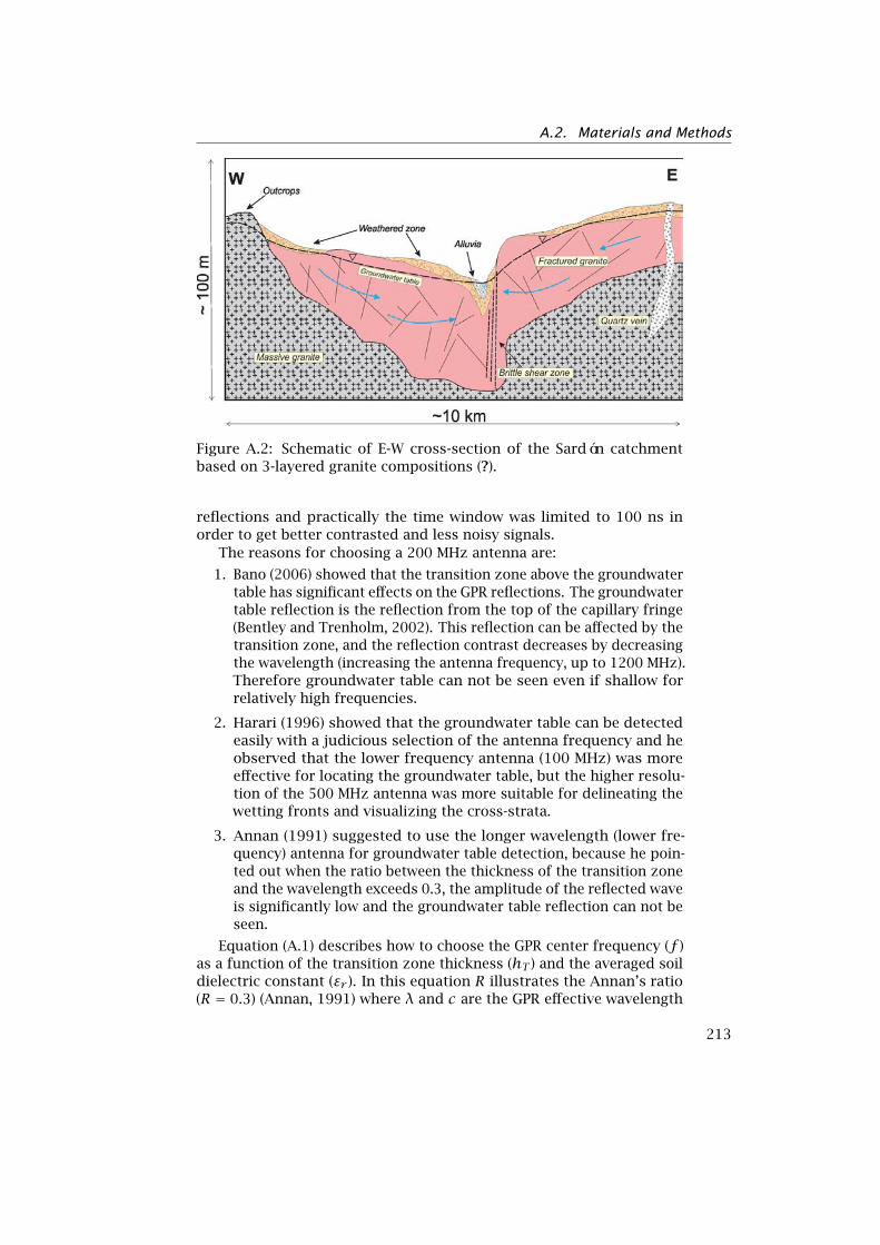
A.2. Materials and Methods
Figure A.2: Schematic of E-W cross-section of the Sardón catchmentbased on 3-layered granite compositions (?).
reflections and practically the time window was limited to 100 ns inorder to get better contrasted and less noisy signals.
The reasons for choosing a 200 MHz antenna are:
1. Bano (2006) showed that the transition zone above the groundwatertable has significant effects on the GPR reflections. The groundwatertable reflection is the reflection from the top of the capillary fringe(Bentley and Trenholm, 2002). This reflection can be affected by thetransition zone, and the reflection contrast decreases by decreasingthe wavelength (increasing the antenna frequency, up to 1200 MHz).Therefore groundwater table can not be seen even if shallow forrelatively high frequencies.
2. Harari (1996) showed that the groundwater table can be detectedeasily with a judicious selection of the antenna frequency and heobserved that the lower frequency antenna (100 MHz) was moreeffective for locating the groundwater table, but the higher resolu-tion of the 500 MHz antenna was more suitable for delineating thewetting fronts and visualizing the cross-strata.
3. Annan (1991) suggested to use the longer wavelength (lower fre-quency) antenna for groundwater table detection, because he poin-ted out when the ratio between the thickness of the transition zoneand the wavelength exceeds 0.3, the amplitude of the reflected waveis significantly low and the groundwater table reflection can not beseen.
Equation (A.1) describes how to choose the GPR center frequency (f )as a function of the transition zone thickness (hT ) and the averaged soildielectric constant (εr ). In this equation R illustrates the Annan’s ratio(R = 0.3) (Annan, 1991) where λ and c are the GPR effective wavelength
213
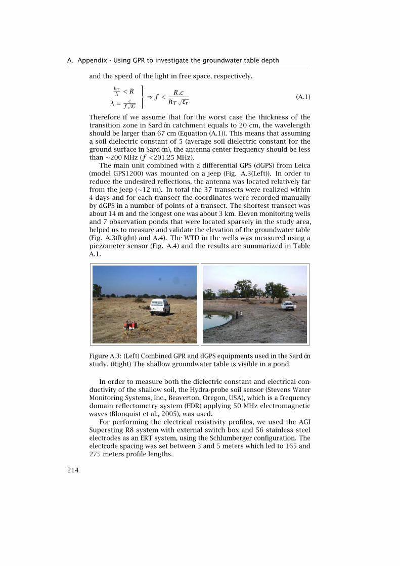
A. Appendix - Using GPR to investigate the groundwater table depth
and the speed of the light in free space, respectively.
hTλ < R
λ = cf√εr
⇒ f < R.chT√εr
(A.1)
Therefore if we assume that for the worst case the thickness of thetransition zone in Sardón catchment equals to 20 cm, the wavelengthshould be larger than 67 cm (Equation (A.1)). This means that assuminga soil dielectric constant of 5 (average soil dielectric constant for theground surface in Sardón), the antenna center frequency should be lessthan ∼200 MHz (f <201.25 MHz).
The main unit combined with a differential GPS (dGPS) from Leica(model GPS1200) was mounted on a jeep (Fig. A.3(Left)). In order toreduce the undesired reflections, the antenna was located relatively farfrom the jeep (∼12 m). In total the 37 transects were realized within4 days and for each transect the coordinates were recorded manuallyby dGPS in a number of points of a transect. The shortest transect wasabout 14 m and the longest one was about 3 km. Eleven monitoring wellsand 7 observation ponds that were located sparsely in the study area,helped us to measure and validate the elevation of the groundwater table(Fig. A.3(Right) and A.4). The WTD in the wells was measured using apiezometer sensor (Fig. A.4) and the results are summarized in TableA.1.
Figure A.3: (Left) Combined GPR and dGPS equipments used in the Sardónstudy. (Right) The shallow groundwater table is visible in a pond.
In order to measure both the dielectric constant and electrical con-ductivity of the shallow soil, the Hydra-probe soil sensor (Stevens WaterMonitoring Systems, Inc., Beaverton, Oregon, USA), which is a frequencydomain reflectometry system (FDR) applying 50 MHz electromagneticwaves (Blonquist et al., 2005), was used.
For performing the electrical resistivity profiles, we used the AGISupersting R8 system with external switch box and 56 stainless steelelectrodes as an ERT system, using the Schlumberger configuration. Theelectrode spacing was set between 3 and 5 meters which led to 165 and275 meters profile lengths.
214

A.2. Materials and Methods
Table A.1: GWTD in the wells and ponds in Sardón. For the location ofeach one refer to Fig. A.1.
ID Type GWTD (m) Groundwater Table elevation (m) Bottom depth (m)
W1 well 2.10 794.88 7.9
W2 well 0.00 803.50 1.6
W3 well 1.51 802.86 2.00
W4 well 1.94 742.13 2.75
W5 well 3.23 739.92 Not Measured
W6 well 2.50 761.82 3.13
W7 well 1.99 803.70 3.36
W8 well dry dry 1.08
W9 well 2.58 805.69 3.65
W10 well dry dry 1.53
W11 well 1.00 733.35 1.8
P1 pond 1.61 806.39 Not Measured
P2 pond 2.27 764.04 Not Measured
P3 pond 4.11 760.71 Not Measured
P4 pond 1.34 765.67 Not Measured
P5 pond 2.01 791.69 Not Measured
P6 pond 1.42 763.11 Not Measured
P7 pond 2.21 814.34 Not Measured
P8 pond 1.56 750.35 Not Measured
A.2.3 Data processing
A.2.3.1 GPR
Variable range gain functions were applied to the data to strengthendeeper reflections. In particular, the automated range gain functionof the system was removed and a power gain function (typically t2.5)was applied. To reduce the effect of the undesired signals such asnoise and clutter, a band pass frequency filter was applied to mostdatasets, with a bandwidth of 95-300 MHz. Y-axis was also transformedto depth instead of travel time using Equation (A.2) for all profiles. In thisequation, dt and t illustrate depth and 2-way travel time, respectively.It is worth noting that for time-depth transformation we used the valueof shallow soil dielectric constant where the exact GWTD informationfrom the observation wells was not available. Otherwise this equation
215
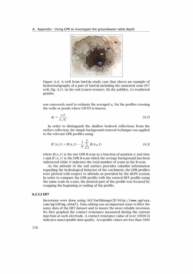
A. Appendix - Using GPR to investigate the groundwater table depth
Figure A.4: A well from Sardón study case that shows an example ofhydrostratigraphy of a part of Sardón including the saturated zone (W7well, Fig. A.1). (a) dry soil (coarse-texture). (b) dry pebbles. (c) weatheredgranite.
was conversely used to estimate the averaged εr for the profiles crossingthe wells or ponds where GWTD is known.
dt =c.t
2√εr
(A.2)
In order to distinguish the shallow bedrock reflections from thesurface reflection, the simple background removal technique was appliedto the relevant GPR profiles using
B′(x, t) = B(x, t)− 1N
N∑n=1
B(xn, t) (A.3)
where B(x, t) is the raw GPR B-scan as a function of position x and timet and B′(x, t) is the GPR B-scan which the average background has beensubtracted while N indicates the total number of scans in the B-scan.
As the altitude of the soil surface provides valuable informationregarding the hydrological behavior of the catchment, the GPR profileswere plotted with respect to altitude as provided by the dGPS system.In order to compare the GPR profile with the existed ERT profile usingthe same scale in x-axis, the desired part of the profile was focused bycropping the beginning or ending of the profile.
A.2.3.2 ERT
Inversions were done using AGI EarthImager2D http://www.agiusa.com/agi2dimg.shtml). Data editing was an important issue to filter thenoisy data of the ERT dataset and to insure the most reliable inversion.We first graphed the contact resistance measured during the currentinjection at each electrode. A contact resistance value of over 10000 Ωindicates unacceptable data quality. Acceptable values are less than 5000
216
A.2. Materials and Methods
Ω, ideally less than 2000 Ω. We selected and removed the electrodeswith all values>10000 Ω and proceeded with the inversion using therobust method and with no limit in the resistivity bounds. The robustinversion was chosen since it was expected sharp boundaries betweenthe unsaturated and saturated zone and between weathered granite orsoil and fresh granite. After the first inversion, we removed all pointswith misfit (RMSE > 50%) and proceeded again the inversion.
The ERT images were obtained by the 2-dimensional cubic interpol-ation of the inverted profiles and plotting with respect to altitude asprovided by the dGPS. In order to compare the ERT profile with GPRprofile using the same scale in x-axis, the desired part of the profile wasfocused by cropping the beginning or ending of the profile.
A.2.4 GPR simulations
In order to provide valuable insights for the radar data interpretation,and in particular better recognize the saturated zone reflection in theGPR images, we used GPR forward modeling by means of GprMax2Dsoftware V 1.5 (Giannopoulos, 2005) to model the sublayers and theGPR reflections. GprMax2D applies the Finite-Difference Time-Domainmethod to solve numerically Maxwell’s equations. For modeling the casestudy, we used the hydrolayer properties summarized in Table A.2. Weconsidered a 4 cm distance between the GPR antenna phase centers(source and receiver) and the ground surface, with a source-receiveroffset of 33 cm. The cell size of the numerical models was assigned2× 2 cm. We used a Ricker pulse with 200 MHz center frequency as anexcitation source. The time window was limited to 100 ns as for the fielddata. A power gain function of time with a factor 2.5 was applied tobetter observe the later reflections compared to the surface reflection.
217

A.
Appen
dix
-U
sing
GPR
toin
vestigate
the
gro
undw
atertab
ledep
th
Table A.2: Measured hydrolayer parameters considered for GPR simulations. The electromagnetic parameters were measuredusing Hydra-probe soil sensor and the thicknesses were measured using drilling and ERT methods.
Layer Stratigraphy σ (mS.m−1) εr Thickness (m)
min max value min max value min max value
Unsaturated soil A 0.67 2.00 1.43 3 9 5 0.0 3.0 2.0
Saturated soil A1 10.0 100 20.0 - - 25 0.0 6.0 1.0
Unsaturated soil pebbles B 1.33 5.00 2.00 7 9 8 0.1 0.5 0.5
Saturated soil pebbles B1 13.33 200 20.0 - - 20 0.1 0.5 0.0
Unsaturated weathered-granite C 1.00 2.00 1.25 5 15 7 0.0 2.0 1.0
Saturated weathered-granite C1 2.50 5.00 4.00 - - 27 5.0 50.0 10.0
Hard-granite D 0.20 0.67 0.50 - - 4 - - 100
21
8
A.3. Results and interpretations
A.3 Results and interpretations
A.3.1 Semi-homogenous layering
GPR profile R1 is located in South-East of the study area with S-N orienta-tion and 263 m long. Observation well (W1), digging, and sampling in thisregion show a semi-homogenous layering with 4 different geological lay-ers including ∼1 m sandy-loam (76% sand, 17% silt, and 7% clay), ∼0.5-∼1m soil pebbles, and both unsaturated and saturated weathered granite(Fig. A.4). Figure A.5(b) represents the simulated GPR signal using corres-ponding configuration shown in Fig. A.5(a) also modeling the capillaryfringe with a height of 6 cm. The observed groundwater table reflectionat ∼48 ns travel time shows the highest amplitude compared to otherreflections above it. Figure A.5(c) shows a part of this GPR profile whichcrosses the well W1. In order to transform the time axis to the depthwe applied Equation (A.2) using the averaged dielectric constant valueof 5 obtained by means of Hydra-probe soil sensor. This GPR profilewas processed using the processing procedure explained in the SectionA.2.3.1. W1 is located at position 78 m of the profile which has a waterlevel depth of 2.10 m measured using the piezometer sensor. This waterlevel on the cross-plot indicates the strong reflections ranging between2-3 m potentially due to the local groundwater table because: (1) basedon GPR simulation this reflection is the strongest one after applying thegain, (2) the groundwater table follows the topography smoothly, andthis reflection is almost horizontal in this part, and (3) the center of thisreflection (negative amplitude) satisfies W1 water level and also shows agood agreement of changing the pressure head around the well whichleads to rise the capillary fringe. Figure A.5(d) shows a part of ERT profileE1 with almost the same orientation of R1 (N20W) and electrode spacingof 3 m. This profile shows 3 different layers which are: (1) the resistiveunsaturated zone with a resistivity of 1000 Ω.m and above which is dryand composed by alluvium material with ∼2 m thickness (the shallowestlayer after 25 m along x-axis), (2) slightly saturated weathered granitewith a resistivity of less than 200 Ω.m, and (3) gradual transition ofsaturated weathered granite to less weathered granite with lower watercontent and the resistivity between 200-1000 Ω.m along the profile after25 m (starting below ∼ 10 m). Comparison of the ERT and GPR profilesshows that the groundwater table reflection is mixed with the weatheredgranite reflection specially at x > 44 m which can lead to an uncertaintyof ∼1 m in detecting the groundwater table reflection. The ERT profilealso shows that in interval of 0-5 and 26-33 m the transition zone isshallow and wide leading to less reflection contrast in the GPR profile.The simulated and measured GPR profiles also show that the geologicalcontact between soil and granite is less visible due to the existence ofthe shallow groundwater table.
219
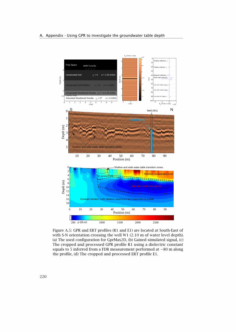
A. Appendix - Using GPR to investigate the groundwater table depth
x (m)
Dep
th (
m)
GPR Tx & RxFree Space
Unsaturated Soil εr = 5 σ = 1.43 mS/m
Unsaturated Soil Pebbles εr = 8 σ = 2 mS/m
Unsaturated Weathered Granite εr=7 σ=1.25 mS/m
Capillary fringe
Saturated Weathered Granite εr = 27 σ = 4 mS/m
0 1 2 3 4 5 6 7 8 9
2.5
2
1
0
x (m)
Dep
th (
m)
Ez (V/m) × t (ns)
4 5
0
1
2
3
4
5−2
−1.5
−1
−0.5
0
0.5
1
x 105
−4 −2 0 2
x 105
0
10
20
30
40
50
60
70
80
90
100
Ez (V/m) × t (ns)
t (n
s)
Surface reflection →
Pebbles reflection →
Bedrock reflection →Water table reflection
2nd−order Pebble ringing →
2nd−order Granite ringing →
2nd−order WT ringing →
Position (m)
Dep
th (
m)
Well (W1)↓
Water level
S N
Shallow and wide water table transition zones
10 20 30 40 50 60 70 80 90
0
1
2
3
4
5
Position (m)
Dep
th (
m)
ρ (Ω.m)
Resistive unsaturated zone
Saturated weathered granite
WT transition zone
Shallow and wide water table transition zones
Gradual transition zone between weathered and unweathered granite
0 10 20 30 40 50 60 70 80 90
02468
1012141618
200 1000 1500 2000 2500
Figure A.5: GPR and ERT profiles (R1 and E1) are located at South-East ofwith S-N orientation crossing the well W1 (2.10 m of water level depth).(a) The used configuration for GprMax2D, (b) Gained simulated signal, (c)The cropped and processed GPR profile R1 using a dielectric constantequals to 5 inferred from a FDR measurement performed at ∼80 m alongthe profile, (d) The cropped and processed ERT profile E1.
220

A.3. Results and interpretations
A.3.2 Heterogeneity effect
Figure A.6(c) shows GPR profile R2 obtained by following R1 with E-Worientation until 312 m in x-axis and S-N orientation from there to theend of profile. The length of this profile is 552 m and it crosses the hill.The hill has 8.17 m height and ∼350 m width with the left hillside slopeof ∼5.14r and right hillside slope of ∼3.09r. R2 was processed same asR1 and it also crosses the well W1. We used the dielectric constant valueof 5 for time-depth transformation. This profile shows a heterogeneoussection of . Figure A.6(a) illustrates the nonhomogeneous configurationwhich was simulated for this area. The modeled configuration is thesame as R1 configuration by replacing the homogeneous pebbles layerwith a nonhomogeneous one. 200 cylinders with random size between10-30 cm diameter and random location with a cave shape and limitedboundary were created to define the nonhomogeneous pebbles layer.Also capillary fringe was modeled with 8 cm height. Figure A.6(b) showsthe B-scan and A-scan of the simulated signal. B-scan is illustrated indepth using a value of 5 for εr (the dielectric constant value of the firstlayer). The groundwater table reflection is visible around 2-2.3 m depth.Although the groundwater table layer is modeled parallel to the surface,the groundwater table reflection is not smooth because of the effect ofthe heterogeneity of pebbles layer. Also this heterogeneity affects on theringings and bedrock reflection, i.e., the bedrock reflection is not visiblein B-scan and some ringings after groundwater table reflection appears.
Thanks to the background removal technique, the reflection in Fig.A.6(c) which is highlighted with the red dashed line shows the weathered/fracturedbedrock. Referring to the drilled well W1 (Fig. A.4), it shows that thefractured granite in this region is shallow (less than 1.5 m depth) andcovered with pebbles. Also W1 shows that the weathered-fractured bed-rock is saturated with water level of 2.10 m depth. Figure A.6(d) focuseson the 70 m of the left hillside also showing W1 as a cross-plot. Thesignificant reflections observed around 2-3 m depth corresponded to themixed saturated sublayer and bedrock reflections. The reflections arenot horizontal probably due to the heterogeneity of the pebbles layer.
A.3.3 The effect of fractures in the saturated granite
R3 is another GPR profile which was carried out in South-West of withW-E orientation and 418 m long. In that area, the fractured granite isshallow and saturated (∼1.5 m depth). Figure A.7(c) shows the processedprofile using topography correction and background removal. Thisprofile crosses 2 wells, namely, W2 and W3. The well W2 which is notdeep enough has 0 m GWTD (not dry), 1.6 m bottom depth and 803.50m groundwater table elevation while W3 has 1.51 m GWTD, 2.00 mbottom depth, and 802.86 m groundwater table elevation. The distancebetween those wells is 29 m with a 32 cm difference in the locationelevation. The groundwater table reflection and cross-plot of the wells areshown in the Figure as well. For time-depth transformation, a dielectric
221
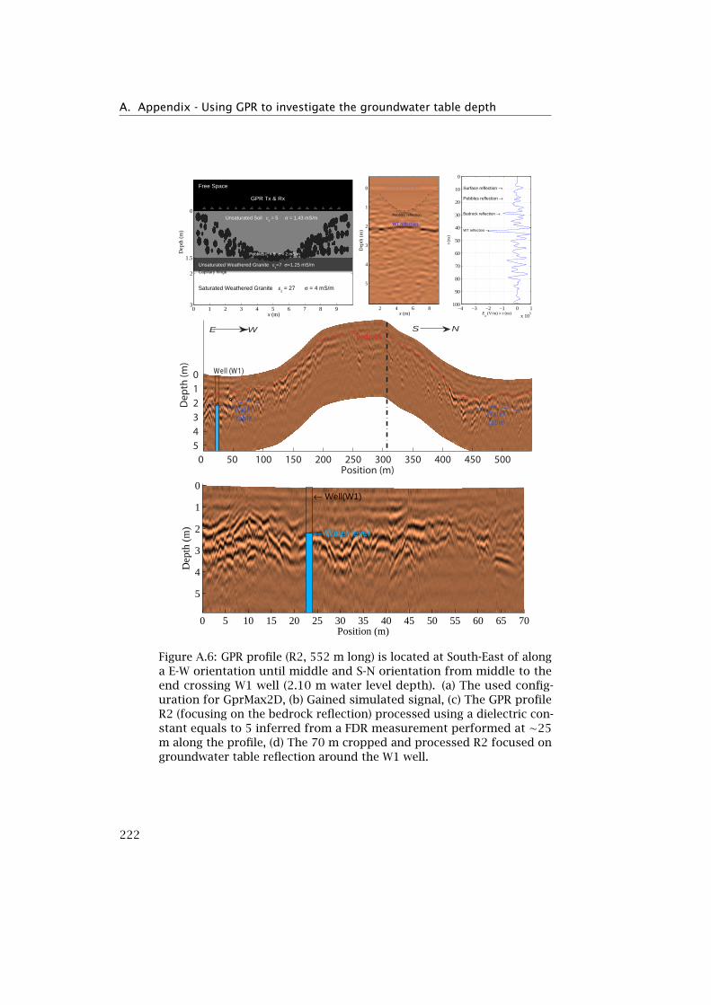
A. Appendix - Using GPR to investigate the groundwater table depth
x (m)
Dep
th (
m)
GPR Tx & Rx
Free Space
Unsaturated Soil εr = 5 σ = 1.43 mS/m
Pebbles εr = 9 σ = 2 mS/m
Unsaturated Weathered Granite εr=7 σ=1.25 mS/m
Capillary fringe
Saturated Weathered Granite εr = 27 σ = 4 mS/m
0 1 2 3 4 5 6 7 8 93
2
1.5
0
Surface reflection
Pebbles reflection
WT reflection
x (m)
Dep
th (
m)
2 4 6 8
0
1
2
3
4
5
−4 −3 −2 −1 0 1
x 105
0
10
20
30
40
50
60
70
80
90
100
Ez (V/m) × t (ns)
t (n
s)
Surface reflection →
Pebbles reflection →
Bedrock reflection →
WT reflection →
Position (m)
Dep
th (m
)
Well (W1)
0 50 100 150 200 250 300 350 400 450 500
0 1 2 3 4 5
Watertable
Watertable
BedrockE W S N
Position (m)
Dep
th (
m)
← Well(W1)
← Water level
0 5 10 15 20 25 30 35 40 45 50 55 60 65 70
0
1
2
3
4
5
Figure A.6: GPR profile (R2, 552 m long) is located at South-East of alonga E-W orientation until middle and S-N orientation from middle to theend crossing W1 well (2.10 m water level depth). (a) The used config-uration for GprMax2D, (b) Gained simulated signal, (c) The GPR profileR2 (focusing on the bedrock reflection) processed using a dielectric con-stant equals to 5 inferred from a FDR measurement performed at ∼25m along the profile, (d) The 70 m cropped and processed R2 focused ongroundwater table reflection around the W1 well.
222

A.3. Results and interpretations
constant value of 6.42 was practically obtained to fit the groundwatertable reflection and existent water levels in the wells (using Equation A.2,conversely). In order to better understand the effect of the saturatedfractured granite, a relevant configuration was modeled including 1 msoil layer, 70 cm weathered granite layer, and saturated fractured graniteusing 400 horizontal tiny fractures randomly located in the relevant layer.Figure A.7(a,b) show the configuration and simulated B-scan and A-scanGPR data, respectively. The result of this simulation shows wheneverthe fractured granite contains water, multiple reflections may occur (Fig.A.7(b)). These multiple reflections may be caused due to the formation ofwaveguides for the short wavelengths. Mostly the wavelength inside thewater is reduced by a factor of nine as compared to the wavelength in theair. These multiple reflections are visible along almost the entire profile.In the position range of 230-300 m the multiple reflections are morevisible and stronger probably because of the presence of the fracturedgranite in this zone, i.e., the bedrock is more fractured in this part.
A.3.4 The clay effect
In the south part of near the pond P4, the GPR profile R4 was carried outwith 290 m long and NW-SE direction. Also in this area the ERT profile E4was carried out with 275 m long (5 m electrode spacing for 56 electrodes)and the same direction as R4. In order to match the GPR and ERTprofiles, they were cropped in x-axis for 265 m long. R4 was processedin the same way as R3 and for time-depth transformation εr=5 was usedpractically. The profiles cross a dry stream at 65 m in x-axis. The lowestand highest elevations are separated by 9.48 m along 120 m long whichleads to an average 4.52r slope for the uphill. The stream channel is filledwith alluvium material and had a low water content during the surveyperiod. Figure A.8(b) shows E4 and illustrates a high conductive area of. Soil sampling showed that this area is covered by weathered granitewith heavy clay which leads to a resistivity of ∼25 Ω.m. E4 also showsthe weathered/fractured granite at a depth of >12 m with maximumresistivity of 350 Ω.m. This amount of resistivity may refer to saturationof the bedrock. The pond P4 is close to the location of 70 m in the x-axisof the profile and had 1.34 m GWTD (Table A.1) which shows that thegroundwater table in this region is relatively shallow. Because of theexistence of the clay in the soil of this region capillary fringe rise is highand leads to no sharp boundary for distinguishing the groundwater tableas well for R4 GPR profile which is shown in Fig. A.8(a). Nevertheless,there are a few different patterns in both ERT and GPR profiles which arediscussed in the following. (1) At the beginning part of E4 a transverseboundary is visible which separates a high conductive part (<50 Ω.m) anda relatively shallower less conductive part (>120 Ω.m). This transverseboundary leads to a transverse reflection on R4 starting at the depth of1.35 m (the expected depth of groundwater table referring to P4) andending ∼4 m depth. This pattern may refer to a different soil texture. (2)A shallow vertical high conductive layer is visible at x = 45 m of E4 which
223

A. Appendix - Using GPR to investigate the groundwater table depth
x (m)
Dep
th (
m)
GPR Tx & Rx
Free Space
Unsaturated Soil εr = 5 σ = 1.43 mS/m
Weathered Granite εr = 15 σ = 2 mS/m
Saturated fractured Granite εr = 27 σ = 4 mS/m
0 1 2 3 4 5 6 7 8 93
1.7
1
0
x (m)
Dep
th (
m)
Surface reflection
Bedrock reflection
WT reflection
2 4 6 8
0
1
2
3
4
5−4 −3 −2 −1 0 1
x 105
0
10
20
30
40
50
60
70
80
90
Ez (V/m) × t (ns)
Surface reflection →
Bedrock reflection →
WT reflection →
t (n
s)
Position (m)
Dep
th (m
)
Well (W2)Well (W3)
0 50 100 150 200 250 300 350 400
0
1
2
3
4
5
Bedrockreflection
Water table reflectio n
W E
Figure A.7: GPR profile (R3, 418 m long) from West to East located inSouth-West of crossing 2 wells and saturated fractured granite zone. (a)The used configuration for GprMax2D, (b) Gained simulated signal, (c)The processed GPR profile R3 using a dielectric constant equals to 6.42inferred manually by fitting the GWTD of the wells (W2 and W3) and thestrong continuous reflection at ∼23 ns.
224
A.3. Results and interpretations
leads to almost a strong multiple reflections in R4 at the same locationand which starts at the depth of 0.5 m. (3) Crossing the stream bed at65 m location leads to a different pattern in E4 because of soil texturaldifference in stream bed compared to the adjacent areas. Thanks to lessclay content of this part, the groundwater table reflection is sharp andvisible at the depth of 1.35 m on R4 profile. We used this reflection andP4 GWTD to estimate the averaged soil dielectric constant (εr=5). (4) Ahigh conductive soil exists at the location around 190 m (resistivity isless than 10 Ω.m) which is relatively close to the surface (E4, Fig. A.8(b)).R4 shows a shallow and sharp reflection at this location which is strongerthan adjacent reflections. (5) At the end of ERT profile after the locationof 245 m an abrupt changing on the soil texture appears (resistivityhigher than 200 Ω.m). This changing of the soil texture leads to lesscapillary rise because of less clay content. A reflection at 1.35 m depthis visible on R4 of this part which is horizontal and may be attributed tothe groundwater table, as compared to the groundwater table reflectionat x = 70 m. The reflection around 3 m depth up to bottom along almostthe entire profile may be caused by the groundwater table ringing andhigh attenuation of GPR signals. These profiles show that clay contentstrongly affects the detection of the groundwater table.
A.3.5 GPR data validation and uncertainties
We represented the topography correction in the GPR data processingsection and we used it for all the GPR profiles. However, the length of theGPR profiles are too long leading to sweep a number of different soil typesand layering in each profile and therefore making it difficult to elucidatethe local horizontal reflections. Also due to the lateral variability in thesoil types, the time-depth transformation of the GPR data is critical onceusing a unique dielectric constant for an entire profile. In that respect wedecided to sweep a short transect containing the known GWTD and witha gradient in the altitude. Figure A.9(b) shows the GPR profile R5 (locatedin the east-south of the study area with 21 m long) that we obtainedclose to the pond P5 to evaluate the groundwater table reflection in theGPR data. The Hydra-probe was used in 3 points along the profile tocollect the electromagnetic properties of the shallow soil and showed aspacial surface dielectric constant variability of 3-24. The processed GPRprofile by means of only topography correction and background removalis shown in the figure. The dielectric constant value of 3.1 (from thesurface of the highest part of profile obtained by FDR) was used for time-depth transformation. The continuous and almost horizontal reflectionbelonging to the groundwater table is clear along the entire profile. Closeto the pond because of changing in the pressure head, the top of thecapillary fringe rises and leads to a groundwater table reflection gradientin the profile as shown in the 0-7 m of x-axis. In order to evaluate thedepth accuracy of the detected reflection and find the total uncertainty ofGWTD detection coming from FDR, dGPS and time-depth transformationmethod we used 2 points along the profile. The points are located at 9
225

A. Appendix - Using GPR to investigate the groundwater table depth
Position (m)
Dep
th (m
)
0 20 40 60 80 100 120 140 160 180 200 220 240 260
0
1
2
3
4 Transversereflection
Verticallayering
Sharp surfacereflection
WT
WT
Different soilstructure
NWSE
Crossing dry stream
Position (m)
Dep
th (m
)
ρ (Ω.m)
0 20 40 60 80 100 120 140 160 180 200 220 240 260
0 5
10152025
0 50 100 150 200 250 300 340
Transverseconductive
layer
Verticalconductive
layerLow conductive
soil
Saturatedweathered/fractured
granite
Crossing dry stream
High conductivesoil
Figure A.8: GPR and ERT profiles (R4 and E4) are located at south part ofin a conductive area with heavy clay content and along a NW-SE (N250W)orientation with about 275 m long for ERT and 290 m long for GPRprofile. (a) The cropped and processed GPR profile using a dielectricconstant equals to 5 inferred manually by fitting the GWTD of the pondP4 and the local horizontal reflection at ∼19 ns located at ∼255 m alongthe profile (this profile crosses the stream at ∼65 m in x-axis), (b) Thecropped ERT profile.
226

A.3. Results and interpretations
and 17 m along the profile having the dielectric constant values of 11.5and 3.1 (obtained by FDR) and the surface elevation values of 792.6 and793.8 m (obtained by dGPS), respectively. The respective groundwatertable reflection times in the unprocessed GPR profile (the raw GPR profileis not presented) are 20 and 25 ns, and the calculated GWTD for thosepoints are 0.88 and 2.12 m, respectively. Assuming that the groundwatertable is horizontal, the difference of the GWTD (∆d) for those pointsshould show the difference of the surface elevation (∆Z) between them.Referring to the calculated GWTD values leads to ∆d = 1.24 m whilethe surface elevation values result ∆Z = 1.2 m. Therefore the resultingerror is 4 cm, which is negligible due to the observational and systematicerrors. It is worth noting that time-depth transformation may lead to asignificant error of GWTD. The processed GPR profile used the lowestvalue of εr (3.1) for time-depth transformation. Referring to the pointwhich is located at x = 9 m shows a GWTD of 1.57 m while the expectedGWTD is 0.88 m and therefore results to a relative error of 57% for GWTD.
227
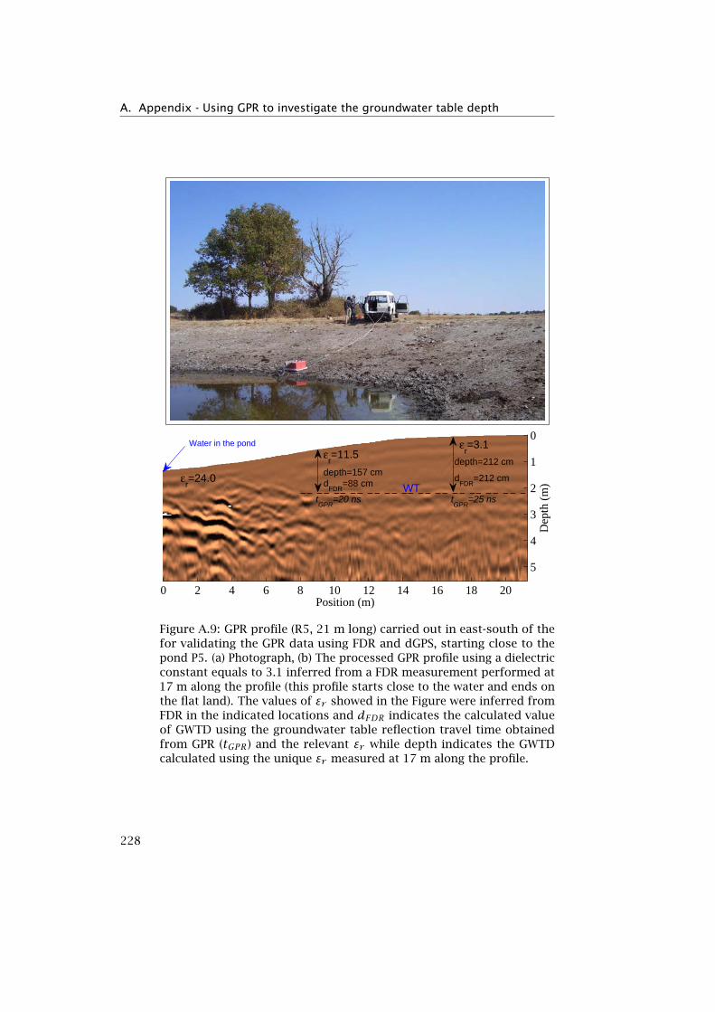
A. Appendix - Using GPR to investigate the groundwater table depth
Position (m)
Dep
th (
m)ε
r=24.0
εr=11.5
εr=3.1
depth=212 cm
dFDR
=212 cmdepth=157 cmd
FDR=88 cm
tGPR
=20 ns tGPR
=25 nsWT
Water in the pond
0 2 4 6 8 10 12 14 16 18 20
0
1
2
3
4
5
Figure A.9: GPR profile (R5, 21 m long) carried out in east-south of thefor validating the GPR data using FDR and dGPS, starting close to thepond P5. (a) Photograph, (b) The processed GPR profile using a dielectricconstant equals to 3.1 inferred from a FDR measurement performed at17 m along the profile (this profile starts close to the water and ends onthe flat land). The values of εr showed in the Figure were inferred fromFDR in the indicated locations and dFDR indicates the calculated valueof GWTD using the groundwater table reflection travel time obtainedfrom GPR (tGPR) and the relevant εr while depth indicates the GWTDcalculated using the unique εr measured at 17 m along the profile.
228
A.4. Conclusions
A.4 Conclusions
This study emphasizes on non-invasive and large scale hydrogeologicalcharacterization and monitoring techniques in order to investigate theGWTD in weathered granites. In that respect, GPR was applied in asemi-arid catchment () in 37 transects with a total length of ∼ 23 km.In this research we found: (1) the shallow groundwater table returnsa strong reflection signal in the GPR images, (2) the geological contactbetween soil and granite is less visible in the GPR profiles in existence ofshallow groundwater table, (3) the groundwater table reflection is almostsmooth and it follows quite well the topography but can be affected bythe heterogeneity of the layering above it, (4) multiple reflections areexpected to happen in presence of saturated fractured granite due to thecreation of visible random waveguides for the radar, (5) clay presencein the soil affects the groundwater table reflections and make themnonvisible because of high capillarity and signal attenuation, (6) time-depth transformation using a single dielectric constant value may lead toa significant error of GWTD, and (7) the groundwater table type is localand it is sparsely distributed in the entire catchment by depth rangingbetween ∼1 to ∼3 m. It is worth noting that the common-mid-point (CMP)method of GPR data acquisition would have improved the estimates ofthe soil dielectric constant where the strong lateral variability in soildielectric constant does not exist. In the future, research will focus onthe full-waveform inversion of the radar data for a more accurate layerreconstruction and interpretation.
229


Bibliography
Al Fugara, A., Pradhan, B., Ahmed Mohamed, T., 2009. Improvement ofland-use classification using object-oriented and fuzzy logic approach.Applied Geomatics 1, 111–120.
Alcalá, F.J., Custodio, E., 2008. Using the Cl/Br ratio as a tracer to identifythe origin of salinity in aquifers in Spain and Portugal. Journal ofHydrology 359, 189–207.
Allen, R.G., Pereira, L., Raes, D., Smith, M., 1998. Crop evapotranspiration:guidelines for computing crop water requirements. Technical Report.Food and Agriculture Organization of the United Nations. Rome.
Almeida, C., Crispim, J., 1987. Traçagens com uranina no Algar doEscarpão (Albufeira, Algarve). ALGAR, Bol. Soc. Portuguesa de Espele-ologia 1, 9–16.
Almeida, C.A.C., Mendonça, J., Jesus, M., Gomes, A., 2000. Sistemasaquíferos de Portugal continental. Technical Report. Centro de Geologiada Faculdade de Ciências de Lisboa and Instituto da Água. Lisbon.
Almeida, C.A.C., Lourenço da Silva, M., 1990. Hidrogeologia do Miocénicoentre Albufeira e Ribeira de Quarteira. Geolis IV, 16.
Andersen, T.R., Poulsen, S.E., Christensen, S., Jørgensen, F., 2012. Asynthetic study of geophysics-based modelling of groundwater flow incatchments with a buried valley. Hydrogeology Journal 20.
Anderson, M.P., Woessner, W.W., 1992. Applied groundwater modeling:simulation of flow and advective transport. Academic Press, San Diego.
Annan, A.P., 1991. Water table detection with ground penetrating radar.61st Ann. Internat. Mtg., Soc. Expl. Geophys., Expanded Abstracts .
Annan, A.P., 2002. GPR-History, trends, and future developments. Sub-surface Sensing Technologies and Applications 3, 253–270.
Archie, G., 1942. Electrical resistivity log as an aid in determining somereservoir characteristics. Petroleum Transactions of AIME 146, 54–61.
Attanayake, A.N.B., 1999. Analysis of fractures in a granitic terrain andtheir tectonic and hydrogeological implications : a study from Sardóncatchment area, Salamanca province, Spain. M.Sc. thesis. ITC-Universityof Twente.
231
Bibliography
Auken, E., Kirkegaard, C., Ribeiro, J., Foged, N., Kok, A., Auken, E.,Kirkegaard, C., Ribeiro, J., Foged, N., Kok, A., 2010. The use of airborneelectromagnetic for efficient mapping of salt water intrusion and out-flow to the sea, in: 21st Salt Water Intrusion Meeting, Azores, Portugal.pp. 53–56.
Aunay, B., Dörfliger, N., Duvail, C., Grelot, F., Le Strat, P., Montginoul, M.,Rinaudo, J.D., 2006. Hydro-socio-economic implications for water man-agement strategies: the case of Roussillon coastal aquifer, in: Colloqueinternational sur la gestion des grands aquifères, 150eme anniversairede la loi de Darcy, 50eme anniversaire de l’AIH (Association Interna-tionale des Hydrogéologues), Bureau de Recherches Géologiques etMinières-BRGM , Gestion de l’Eau, Acteurs et Usages-UMR G-EAU.
Aunay, B., Dörfliger, N., Duvail, C., Grelot, F., Le Strat, P., Montginoul,M., Rinaudo, J.D., 2007. A multidisciplinary approach for assessingthe risk of seawater intrusion in coastal aquifers: The case of theRoussillon basin (France), in: Aquifer Systems Management: Darcy’sLegacy in a World of Impending Water Shortage: Selected Papers onHydrogeology 10, p. 459.
Basokur, A.T., Akça, I., Siyam, N.W., 2007. Hybrid genetic algorithmsin view of the evolution theories with application for the electricalsounding method. Geophysical Prospecting 55, 393–406.
Baden Ghijben, W., 1888-1889. Nota in verband met de voorgenomenput boring nabij amsterdam. Koninkhijk Institut van Ingenieurs 8.
Baird, K.J., Maddock III, T., 2005. Simulating riparian evapotranspiration:a new methodology and application for groundwater models. Journalof Hydrology 312, 176–190.
Bakker, M., Schaars, F., 2005. The Sea Water Intrusion (SWI) packagemanual Part I: Theory user manual and example, version 1.2. TechnicalReport. University of Georgia and Artesia Water Research.
Baltassat, J.M., Legchenko, A., Ambroise, B., Mathieu, F., Lachassagne, P.,Wyns, R., Mercier, J.L., Schott, J.J., 2005. Magnetic resonance sounding(MRS) and resistivity characterisation of a mountain hard rock aquifer:the Ringelbach catchment, Vosges Massif, France. Near Surface Geo-physics 3, 267–274.
Balugani, E., Lubczynski, M.W., Metselaar, K., 2014. A framework forsourcing of evaporation between saturated and unsaturated zone inbare soil condition. Hydrological Sciences Journal .
Balugani, E., Reyes-Acosta, J.L., van der Tol, C., Lubczynski, M.W., Metse-laar, K., 2015. Groundwater and unsaturated zone evaporation andtranspiration in a semiarid open woodland. Water Resource ResearchSubmitted.
Bano, M., 2006. Effects of the transition zone above a water table on thereflection of GPR waves. Geophysical Research Letters 33, 5.
232
Bibliography
Banta, E., 2000. MODFLOW-2000, the U.S. Geological Survey modularground-water model - Documentation of packages for simulating evapo-transpiration with a segmented function (ETS1) and drains with returnflow (DRT1). Technical Report 00-466. U.S. Geological Survey.
Barazzuoli, P., Nocchi, M., Rigati, R., Salleolini, M., 2008. A conceptualand numerical model for groundwater management: a case study on acoastal aquifer in southern Tuscany, Italy. Hydrogeology Journal 16,1557–1576.
Baroncini-Turricchia, G., Francés, A.P., Lubczynski, M.W., Martínez-Fernández, J., Roy, J., 2014. Integrating MRS data with hydrologicmodel-Carrizal catchment (Spain). Near Surface Geophysics 12.
Batelaan, O., De Smedt, F., 2004. SEEPAGE, a new MODFLOW DRAINpackage. Ground Water 42, 576–588.
Batelaan, O., De Smedt, F., Triest, L., 2003. Regional groundwater dis-charge: phreatophyte mapping, groundwater modelling and impactanalysis of land-use change. Journal of Hydrology 275, 86–108.
Batelaan, O., de Smedt, F., 2007. GIS-based recharge estimation bycoupling surface-subsurface water balances. Journal of Hydrology 337,337–355.
Bauer-Gottwein, P., Gondwe, B.N., Christiansen, L., Herckenrath, D., Kgotl-hang, L., Zimmermann, S., 2010. Hydrogeophysical exploration ofthree-dimensional salinity anomalies with the time-domain electromag-netic method (TDEM). Journal of Hydrology 380, 318–329.
Bear, J., Verruijt, A., 1987. Modeling Groundwater Flow and Pollution.Theory and Applications of Transport in Porous Media, Springer Neth-erlands.
Bentley, L.R., Trenholm, N.M., 2002. The accuracy of water table elevationestimates determined from ground penetrating radar data. Journal ofEnvironmental and Engineering Geophysics 7, 37–53.
Benz, U.C., Hofmann, P., Willhauck, G., Lingenfelder, I., Heynen, M., 2004.Multi-resolution, object-oriented fuzzy analysis of remote sensingdata for GIS-ready information. ISPRS Journal of Photogrammetry andRemote Sensing 58, 239–258.
Bernard, J., 2007. Instruments and field work to measure a magneticresonance sounding. Boletín Geológico y Minero 118 (3), 459–472.
Beven, K., Freer, J., 2001. A dynamic TOPMODEL. Hydrological Processes15, 1993–2011.
Binley, A., Hubbard, S.S., Huisman, J.A., Revil, A., Robinson, D.A., Singha,K., Slater, L.D., 2015. The emergence of hydrogeophysics for improvedunderstanding of subsurface processes over multiple scales. WaterResources Research 51.
Bishop, T.F.A., McBratney, A.B., 2001. A comparison of prediction meth-ods for the creation of field-extent soil property maps. Geoderma 103,149–160.
233
Bibliography
Blonquist, J.M., Jones, S.B., Robinson, D.A., 2005. Standardizing charac-terization of electromagnetic water content sensors: Part 2. evaluationof seven sensing systems. Vadose Zone Journal 4, 1059–1069.
Boucher, M., Costabel, S., Yaramanci, U., 2011. The detectability of waterby NMR considering the instrumental dead time - a laboratory analysisof unconsolidated materials. Near Surface Geophysics 9, 145–153.
Boucher, M., Favreau, G., Descloitres, M., Vouillamoz, J.M., Massuel, S.,Nazoumou, Y., Cappelaere, B., Legchenko, A., 2009a. Contribution ofgeophysical surveys to groundwater modelling of a porous aquiferin semiarid Niger: An overview. Comptes Rendus-Géoscience 341,800–809.
Boucher, M., Favreau, G., Nazoumou, Y., Cappelaere, B., Massuel, S.,Legchenko, A., 2012. Constraining groundwater modeling with mag-netic resonance soundings. Ground Water 50, 775–784.
Boucher, M., Favreau, G., Vouillamoz, J.M., Nazoumou, Y., Legchenko,A., 2009b. Estimating specific yield and transmissivity with magneticresonance sounding in an unconfined sandstone aquifer (Niger). Hy-drogeology Journal 17, 1805–1815.
Bourennane, H., King, D., 2003. Using multiple external drifts to estimatea soil variable. Geoderma 114, 1–18.
Bourennane, H., King, D., Couturier, A., 2000. Comparison of kriging withexternal drift and simple linear regression for predicting soil horizonthickness with different sample densities. Geoderma 97, 255–271.
Braz Teixeira, S.a., Macedo, F., 2001. Prospecção de manchas de em-préstimo ao largo de Albufeira (Algarve). Technical Report. DireçãoRegional do Ambiente e do Ordenamento do Território do Algarve.
Bronzini, S., 2011. Etude hydrogéologique de la zone d’Albufeira (Algarve,Portugal) et analyse des mécanismes de salinisation des eaux souter-raines. Master’s thesis. Université de Neuchâtel. CHYN, Switzerland.
Brunner, P., Simmons, C.T., 2012. Hydrogeosphere: A fully integrated,physically based hydrological model. Ground Water 50, 170–176.
Brunner, P., Simmons, C.T., Cook, P.G., Therrien, R., 2010. Modelingsurface water-groundwater interaction with MODFLOW: Some consid-erations. Ground Water 48, 174–180.
Brus, D.J., Knotters, M., van Dooremolen, W.A., van Kernebeek, P., vanSeeters, R.J.M., 1992. The use of electromagnetic measurements ofapparent soil electrical conductivity to predict the boulder clay depth.Geoderma 55, 79–93.
Burschil, T., Scheer, W., Kirsch, R., Wiederhold, H., 2012. Compiling geo-physical and geological information into a 3-D model of the glacially-affected island of Föhr. Hydrology and Earth System Sciences 16,3485–3498.
Butler, J.J., Healey, J.M., 1998. Relationship between pumping-test andslug-test parameters: Scale effect or artifact? Ground Water 36, 305–312.
234

Bibliography
Cardoso, J.C., 1965. Os solos de Portugal I-A Sul do Rio Tejo.
Carvalho, J., Ramalho, E., Dias, R., Pinto, C., Ressurreição, R., 2012. Ageophysical study of the Carcavai fault zone, Portugal. Pure andApplied Geophysics 169, 183–200.
Carvalho, J., Torres, L., Rocha, R., Dias, R., Mendes-Victor, L., 2006. Ageophysical study of the S. Marcos-Quarteira fault, Portugal. Journalof Applied Geophysics 60, 153–164.
Ceballos, A., Martínez-Fernández, J., Santos, F., Alonso, P., 2002. Soil-water behaviour of sandy soils under semi-arid conditions in the DueroBasin (Spain). Journal of Arid Environments 51, 501–519.
Chandra, S., Ahmed, S., Ram, A., Dewandel, B., 2008. Estimation of hardrock aquifers hydraulic conductivity from geoelectrical measurements:A theoretical development with field application. Journal of Hydrology357, 218–227.
Chaudhuri, A., Sekhar, M., Descloitres, M., Godderis, Y., Ruiz, L., Braun, J.,2013. Constraining complex aquifer geometry with geophysics (2-DERT and MRS measurements) for stochastic modelling of groundwaterflow. Journal of Applied Geophysics 98, 288–297.
Chevalier, A., Legchenko, A., Girard, J., Descloitres, M., 2014. MonteCarlo inversion of 3D magnetic resonance measurements. GeophysicalJournal International 198, 216–228.
Christiansen, A., Auken, E., Søorensen, K., 2009. The transient electro-magnetic method, in: Kirsch, R. (Ed.), Groundwater Geophysics: ATool For Hydrogeology. Springer Berlin Heidelberg. book section 6, pp.179–226.
Chung, I.M., Kim, N.W., Lee, J., Sophocleous, M., 2010. Assessing dis-tributed groundwater recharge rate using integrated surface water-groundwater modelling: application to Mihocheon watershed, SouthKorea. Hydrogeology Journal 18, 1253–1264.
Cook, P.G., 2003. A guide to regional groundwater flow in fracturedaquifers. CSIRO.
Cornillon, P.A., Guyader, A., Husson, F., Jégou, N., Josse, J., Kloareg,M., Matzner-Løber, E., Rouviére, L., 2008. Statistique avec R. PressesUniversitaires de Rennes.
Cortez, R., 2004. Recharge assessment and groundwater modelling ofthe Pisões aquifer (Beja-Portugal). M.sc. thesis. ITC.
Corwin, D.L., Lesch, S.M., 2003. Application of soil electrical conductivityto precision agriculture: Theory, principles, and guidelines. Agron J95, 455–471.
Corwin, D.L., Lesch, S.M., 2005a. Apparent soil electrical conductivitymeasurements in agriculture. Computers and Electronics in Agriculture46, 11–43.
Corwin, D.L., Lesch, S.M., 2005b. Characterizing soil spatial variabilitywith apparent soil electrical conductivity: I. survey protocols. Com-puters and Electronics in Agriculture 46, 103–133.
235

Bibliography
Costabel, S., Yaramanci, U., 2011. Relative hydraulic conductivity andeffective saturation from Earth’s field nuclear magnetic resonance : amethod for assessing the vadose zone. Near Surface Geophysics 9, 155– 167.
Costabel, S., Yaramanci, U., 2013. Estimation of water retention para-meters from nuclear magnetic resonance relaxation time distributions.Water Resources Research 49, 2068–2079.
Creel, L., 2003. Ripple effects: population and coastal regions. Makingthe link .
Custodio, E., 2010. Coastal aquifers of Europe: an overview. Hydrogeo-logy Journal 18, 269–280.
Dam, D., Christensen, S., 2003. Including geophysical data in groundwatermodel inverse calibration. Ground Water 41, 178–189.
Dams, J., Salvadore, E., van Daele, T., Ntegeka, V., Willems, P., Batelaan, O.,2012. Spatio-temporal impact of climate change on the groundwatersystem. Hydrology and Earth System Sciences 16, 1517–1531.
Danielsen, J., Dahlin, T., Owen, R., Mangeya, P., Auken, E., 2007. Geo-physical and hydrogeologic investigation of groundwater in the Karoostratigraphic sequence at Sawmills in northern Matabeleland, Zimb-abwe: a case history. Hydrogeology Journal 15, 945–960.
Danielsen, J.E., Auken, E., Jørgensen, F., Søndergaard, V., Sørensen, K.I.,2003. The application of the transient electromagnetic method inhydrogeophysical surveys. Journal of Applied Geophysics 53, 181–198.
David, T., Ferreira, M., Cohen, S., Pereira, J., David, J., 2004. Constraintson transpiration from an evergreen oak tree in southern Portugal.Agricultural and Forest Meteorology 122, 193–205.
Davies, G., Huang, J., Monteiro Santos, F.A., Triantafilis, J., 2014. Modelingcoastal salinity in quasi 2D and 3D using a dualem-421 and inversionsoftware. Groundwater 53, 424–431.
DeMeo, G.A., Laczniak, R.J., Boyd, R.A., Smith, J.L., Nylund, W.E., 2003.Estimated ground-water discharge by evapotranspiration from DeathValley, California, 1997-2001. Technical Report. U.S. Geological Survey.
Descloitres, M., Ruiz, L., Sekhar, M., Legchenko, A., Braun, J.J., Kumar,M.S.M., Subramanian, S., 2008. Characterization of seasonal local re-charge using electrical resistivity tomography and magnetic resonancesounding. Hydrological Processes 22, 384–394.
Dewandel, B., Lachassagne, P., Wyns, R., Maréchal, J.C., Krishnamurthy,N.S., 2006. A generalized 3-D geological and hydrogeological con-ceptual model of granite aquifers controlled by single or multiphaseweathering. Journal of Hydrology 330, 260–284.
Dewandel, B., Lachassagne, P., Zaidi, F.K., Chandra, S., 2011. A concep-tual hydrodynamic model of a geological discontinuity in hard rockaquifers: Example of a quartz reef in granitic terrain in south India.Journal of Hydrology 405, 474–487.
236
Bibliography
Dewandel, B., Maréchal, J., Bour, O., Ladouche, B., Ahmed, S., Chandra,S., Pauwels, H., 2012. Upscaling and regionalizing hydraulic conduct-ivity and effective porosity at watershed scale in deeply weatheredcrystalline aquifers. Journal of Hydrology 416-417, 83–97.
Dias, J.M.A., Boski, T., Rodrigues, A., Magalhães, F., 2000. Coast lineevolution in Portugal since the Last Glacial Maximum until present-asynthesis. Marine Geology 170, 177–186.
Dingman, S.L., 2002. Physical hydrology. Prentice Hall, Upper SaddleRiver. Second edition.
Doherty, J., 2005. PEST, Model-Independent Parameter Estimation. UserManual: 5th Edition. Watermark Numerical Computing, Brisbane,Australia.
Doherty, J., 2015. Calibration and Uncertainty Analysis for ComplexEnvironmental Models. PEST: complete theory and what it means formodelling the real world. Watermark Numerical Computing.
Domenico, P.A., Schwartz, F., 1998. Physical and chemical hydrogeology.Wiley.
Doolittle, J.A., Jenkinson, B., Hopkins, D., Ulmer, M., Tuttle, W., 2006.Hydropedological investigations with ground-penetrating radar (gpr):Estimating water-table depths and local ground-water flow pattern inareas of coarse-textured soils. Geoderma 131, 317–329.
Doolittle, J.A., Minzenmayer, F.E., Waltman, S.W., Benham, E.C., Tuttle,J.W., Peaslee, S.D., 2007. Ground-penetrating radar soil suitability mapof the conterminous united states. Geoderma 141, 416–421.
Doolittle, J.A., Sudduth, K.A., Kitchen, N.R., Indorante, S.J., 1994. Estim-ating depths to claypans using electromagnetic induction methods.Journal of Soil and Water Conservation 49, 572–575.
Dörfliger, N., 2013. Entre terre et mer, les eaux souterraines du littoral.Géosciences (BRGM) 17, 74–81.
Douglas-Mankin, K., Srinivasan, R., Arnold, J., 2010. Soil and Water As-sessment Tool (SWAT) model: Current developments and applications.Transactions of the ASABE 53, 8.
Dutta, S., Krishnamurthy, N.S., Arora, T., Rao, V.A., Ahmed, S., Baltassat,J.M., 2006. Localization of water bearing fractured zones in a hardrock area using integrated geophysical techniques in Andhra Pradesh,India. Hydrogeology Journal 14, 760–766.
Elsendoorn, B., Hoogeveen, H., Vuyck, P., 1982. Geo-electrisch onderzoekvan de Miocene aquifer tussen Olhos de Agua en Quarteira, Algarve(Portugal). Technical Report. VU University, Faculty of Earth and LifeSciences. Amsterdam.
Encarnação, J.a., Leitão, F., Range, P., Piló, D., Chícharo, M.A., Chícharo, L.,2013. The influence of submarine groundwater discharges on subtidalmeiofauna assemblages in south Portugal (Algarve). Estuarine, Coastaland Shelf Science 130, 202–208.
237
Bibliography
Ernstson, K., Kirsch, R., Janik, M., Krummel, H., 2009. Geoelectricalmethods, in: Kirsch, R. (Ed.), Groundwater Geophysics: A Tool ForHydrogeology. Springer Berlin Heidelberg. chapter 3, pp. 85–117.
Faneca Sanchez, M., Gunnink, J.L., van Baaren, E.S., Oude Essink, G.,Siemon, B., Auken, E., Elderhorst, W., de Louw, P., 2012. Modellingclimate change effects on a dutch coastal groundwater system usingairborne electromagnetic measurements. Hydrology and Earth SystemSciences 16, 4499–4516.
Faraway, J., 2002. Practical Regression and Anova using R. http://cran.r-project.org.
Faraway, J., 2009. faraway: Functions and datasets for books by JulianFaraway. R package version 1.0.4.
Fetter, C., 2001. Applied Hydrogeology. Prentice Hall.
Fienen, M.N., Hunt, R.J., 2015. High-throughput computing versus high-performance computing for groundwater applications. Groundwater53, 180–184.
Finch, J.W., 1998. Estimating direct groundwater recharge using a simplewater balance model-sensitivity to land surface parameters. Journal ofHydrology 211, 112–125.
Finch, J.W., 2001. Estimating change in direct groundwater recharge usinga spatially distributed soil water balance model. Quarterly Journal ofEngineering Geology and Hydrogeology 34, 71–83.
Fleury, P., Bakalowicz, M., de Marsily, G., 2007. Submarine springs andcoastal karst aquifers: A review. Journal of Hydrology 339, 79–92.
Food and Agriculture Organization, 2006. Guidelines for soil description.Technical Report. Food and Agriculture Organization of the UnitedNations. Rome.
Food and Agriculture Organization, 2009. CROPWAT, a computer pro-gram for irrigation planning and management.
Fox, J., 2002. R and S-Plus companion to applied regression. Sage,Thousand Oaks.
Fox, J., Weisberg, S., 2011. An R Companion to Applied Regression. Sage,Thousand Oaks CA. Second edition.
Francés, A.P., 2008. Spatio-temporal groundwater recharge assessment:a data-integration and modelling approach. M.Sc. thesis. ITC-Universityof Twente.
Francés, A.P., Lubczynski, M.W., 2011. Topsoil thickness prediction atthe catchment scale by integration of invasive sampling, surface geo-physics, remote sensing and statistical modeling. Journal of Hydrology405, 31–47.
Francés, A.P., Lubczynski, M.W., 2015. Partitioning and sourcing ofevapotranspiration at the catchment scale using coupled MARMITES-MODFLOW model. Water Resource Research Submitted.
238

Bibliography
Francés, A.P., Lubczynski, M.W., Roy, J., Monteiro Santos, F.A., Mahmoudz-adeh, M.R., 2014. Hydrogeophysics and remote sensing for the designof hydrogeological conceptual models in hard rocks-Sardón catchment(Spain). Journal of Applied Geophysics 110, 63–81.
Francés, A.P., Ramalho, E., Fernandes, J., Groen, M., Hugman, R., Khalil,M.A., De Plaen, J., Monteiro Santos, F.A., 2015. Contributions of hydro-geophysics to the hydrogeological conceptual model of the Albufeira-Ribeira de Quarteira coastal aquifer in Algarve, Portugal. HydrogeologyJournal Accepted (April 2015).
Francese, R., Mazzarini, F., Bistacchi, A., Morelli, G., Pasquarè, G., Praticelli,N., Robain, H., Wardell, N., Zaja, A., 2009. A structural and geophysicalapproach to the study of fractured aquifers in the Scansano-Maglianoin Toscana Ridge, southern Tuscany, Italy. Hydrogeology Journal 17,1233–1246.
Friedman, S.P., 2005. Soil properties influencing apparent electricalconductivity: a review. Computers and Electronics in Agriculture 46,45–70.
Fukushima, E., Roeder, S., 1981. Experimental Pulse NMR: A Nuts andBolts Approach. Addison-Wesley.
Furman, A., 2008. Modeling coupled surfacesubsurface flow processes:A review. Vadose Zone Journal 7, 741–756.
Gash, J.H.C., 1979. An analytical model of rainfall interception by forests.Quarterly Journal of the Royal Meteorological Society 105, 43–55.
Gash, J.H.C., Lloyd, C.R., Lachaud, G., 1995. Estimating sparse forestrainfall interception with an analytical model. Journal of Hydrology170, 79–86.
Gassman, P.W., Reyes, M.R., Green, C.H., Arnold, J.G., 2007. The Soiland Water Assessment Tool: Historical development, applications, andfuture research directions. Transactions of the ASABE 50, 39.
Gehrels, J., 2000. Groundwater level fluctuations. Ph.D. thesis. FreeUniversity of Amsterdam.
Gehrels, J.C., Gieske, A.S.M., 2003. Aquifer dynamics, in: Simmers, I.(Ed.), Understanding water in a Dry Environment-Hydrological pro-cesses in arid and semi-arid zones. Balkema, Rotterdam. volume 23 ofInternational Contributions to Hydrogeology, pp. 211–250.
Geirnaert, W., van Beeres, P., de Vries, J., Hoogeveen, H., 1982. Hydrogeo-logic studies in the East Algarve, Portugal. Part I: Geo-electric survey ofthe miocene aquifer between Quarteira and Olhao, Algarve, Portugal,in: III Semana de Hidrogeologia, 10-14 May, Lisbon, Portugal. pp. 2–22.
Geotomo software, 2010. RES2DINV ver. 3.59-Rapid 2-D resistivity andIP inversion using the least-squares method.
Giannopoulos, A., 2005. Modelling ground penetrating radar by GPRMax.Construction and Building Materials 19, 755–762.
239

Bibliography
Gieske, A., 2003. Operational solutions of actual evapotranspiration, in:Simmers, I. (Ed.), Understanding water in a dry environment : hydro-logical processes in arid and semi arid zones. Balkema, Rotterdam.volume 23, pp. 65–114.
Glover, R.E., 1959. The pattern of fresh-water flow in a coastal aquifer.Journal of Geophysical Research 64, 457–459.
Goldman, M., Gilad, D., Ronen, A., Mellow, A., 1991. Mapping of seawaterintrusion into the coastal aquifer of Israel by time domain electromag-netic method. Geoexploration 28, 153–174.
van de Griend, A.A., Owe, M., 1994. Bare soil surface resistance toevaporation by vapor diffusion under semiarid conditions. WaterResources Research 30, 181–188.
Guan, H., Wilson, J.L., 2009. A hybrid dual-source model for potentialevaporation and transpiration partitioning. Journal of Hydrology 377,405–416.
Habtemariam, T.B., 2000. Subsurface characterization of granitic base-ment from structural and resistivity data : a case study from Sardóncatchment area, Salamanca, Spain. M.Sc. thesis. ITC-University ofTwente.
Harari, Z., 1996. Ground-penetrating radar (GPR) for imaging strati-graphic features and groundwater in sand dunes. Journal of AppliedGeophysics 36, 43–52.
Harbaugh, A., 2005. MODFLOW-2005, the U.S. Geological Survey modularground-water model - the Ground-Water Flow Process. Technical Report6-A16. U.S. Geological Survey.
Harbaugh, A., Banta, E., Hill, M., Mc Donald, M., 2000. MODFLOW-2000,the U.S. Geological Survey modular ground-water model - User guideto modularization concepts and the Ground-Water Flow Process. Tech-nical Report 00-92. U.S. Geological Survey.
Hassan, S.T., Lubczynski, M.W., Niswonger, R.G., Su, Z., 2014. Surface-groundwater interactions in hard-rocks in Sardón catchment of West-ern Spain: an integrated modeling approach. Journal of Hydrology 517,390–410.
Henderson, R.D., Day-Lewis, F.D., Abarca, E., Harvey, C.F., Karam, H.N.,Liu, L., Lane, John W., J., 2010. Marine electrical resistivity imaging ofsubmarine groundwater discharge: sensitivity analysis and applicationin Waquoit Bay, Massachusetts, USA. Hydrogeology Journal 18, 173–185.
Hendricks, J.M.H., Phillips, F.M., Harrison, J.B., 2003. Water flow processesin arid and semi-arid vadose zones, in: Simmers, I.e. (Ed.), Understand-ing water in a Dry Environment - Hydrological processes in arid andsemi-arid zones. Balkema. volume 23 of International Contributions toHydrogeology. chapter 5, pp. 151–210.
Hengl, T., 2009. A Practical Guide to Geostatistical Mapping. Universityof Amsterdam, www.lulu.com. Second edition.
240
Bibliography
Hengl, T., Gruber, S., Shrestha, D.P., 2003a. Digital terrain analysis inILWIS : lecture note. Technical Report. ITC.
Hengl, T., Rossiter, D.G., Stein, A., 2003b. Soil sampling strategies for spa-tial prediction by correlation with auxiliary maps. Australian Journalof Soil Research 41, 1403–1422.
Herckenrath, D., 2012. Informing groundwater models with near-surfacegeophysical data. Ph.D. thesis. Department of Environmental Engineer-ing, Technical University of Denmark.
Hertrich, M., 2008. Imaging of groundwater with nuclear magnetic res-onance. Progress in Nuclear Magnetic Resonance Spectroscopy 53,227–248.
Herzberg, B., 1901. Die wasserversorgung einiger nordssbader. J. Gas-beleuch. Wasservers , 815–819 and 842–844.
Hill, M., Tiedeman, C., 2006. Effective Groundwater Model Calibration:With Analysis of Data, Sensitivities, Predictions, and Uncertainty. Wiley.
Hiscock, K., Bense, V., 2014. Hydrogeology: Principles and Practice. Wiley.
Holländer, H.M., Wang, Z., Assefa, K.A., Woodbury, A.D., 2015. Improvedrecharge estimation from portable, low-cost weather stations. Ground-water .
Houser, P.R., Shuttleworth, W.J., Famiglietti, J.S., Gupta, H.V., Syed, K.H.,Goodrich, D.C., 1998. Integration of soil moisture remote sensingand hydrologic modeling using data assimilation. Water ResourcesResearch 34, 3405–3420.
Hugman, R., Stigter, T.Y., Monteiro, J.P., 2014a. Developing a 3-D variabledensity numerical model for a heavily exploited coastal aquifer withsubmarine spring discharge - South Portugal, in: IAH (Ed.), 41st IAHInternational Congress "Groundwater : Challenges and Strategies",Marrakech.
Hugman, R., Stigter, T.Y., Monteiro, J.P., Costa, L., Nunes, L.M., 2014b.Modeling the spatial and temporal distribution of coastal groundwaterdischarge for different water use scenarios under epistemic uncer-tainty: case study in south portugal. Environmental Earth Sciences 73,2657–2669.
Hunt, R.J., Luchette, J., Schreuder, W.A., Rumbaugh, J.O., Doherty, J.,Tonkin, M.J., Rumbaugh, D.B., 2010. Using a cloud to replenish parchedgroundwater modeling efforts. Ground Water 48, 360–365.
Illman, W.A., 2006. Strong field evidence of directional permeability scaleeffect in fractured rock. Journal of Hydrology 319, 227–236.
Instituto Geológico y Minero de España, 1978. Mapa geológico de Españaa escala 1:50 000. Hoja 426 (Fuentesauco).
Instituto Geológico y Minero de España, 1991a. Mapa geológico de Españaa escala 1:50 000. Hoja 450 (Vitigudino).
Instituto Geológico y Minero de España, 1991b. Mapa geológico de Españaa escala 1:50 000. Hoja 451 (Ledesma).
241

Bibliography
Instituto Geológico y Minero de España, 2000. Mapa geológico de Españaa escala 1:50 000. Hoja 425 (Villamor de los Escuderos).
Jackson, T.J., Schmugge, J., Engman, E.T., 1996. Remote sensing applica-tions to hydrology: soil moisture. Hydrological Sciences 41, 517–530.
Jenness, J., 2006. Topographic Position Index (tpi_jen.avx) extension forArcView 3.x.
Johnson, E., Yáñez, J., Ortiz, C., Muñoz, J., 2010. Evaporation from shal-low groundwater in closed basins in the chilean altiplano. HydrologicalSciences Journal 55, 624–635.
Jyrkama, M., Sykes, J., Normani, S., 2002. Recharge estimation for transi-ent groundwater modeling. Ground Water 40, 638–648.
Keller, G.V., Frischknecht, F.C., 1966. Electrical methods in geophysicalprospecting. Pergamon Press, Inc.
Kim, N.W., Chung, I.M., Won, Y.S., Arnold, J.G., 2008. Developmentand application of the integrated SWAT-MODFLOW model. Journal ofHydrology 356, 1–16.
Kinzelbach, W., Aeschbach, W., Alberich, C., Goni, I., Beyerle, U., Brunner,P., Chiang, W., Rueedi, J., Zollmann, K., 2002. A survey of methods forgroundwater recharge in arid and semi-arid regions. Early Warningand Assessment Report Series UNEP/DEWA/RS.02-2, Nairobi, Kenya.
Kirsch, R. (Ed.), 2009. Groundwater Geophysics: A Tool For Hydrogeology.Springer, Berlin. 2nd edition.
Kirsch, R., Yaramanci, U., 2009. Geophysical characterisation of aquifers,in: Kirsch, R. (Ed.), Groundwater Geophysics: A Tool For Hydrogeology.Springer Berlin Heidelberg. book section 17, pp. 491–509.
Kite, G., 2000. Using a basin-scale hydrological model to estimate croptranspiration and soil evaporation. Journal of hydrology 229, 59–69.
Knotters, M., Brus, D.J., Oude Voshaar, J.H., 1995. A comparison ofkriging, co-kriging and kriging combined with regression for spatialinterpolation of horizon depth with censored observations. Geoderma67, 227–246.
Kok, A., Auken, E., Groen, M., Riberio, J., Shaars, F., 2010. Using groundbased geophysics and airborne transient electromagnetic measure-ments (SkyTEM) to map salinity distribution and calibrate a groundwa-ter model for the island of Terschelling-The Netherlands, in: 21st SaltWater Intrusion Meeting, Azores, Portugal.
Kollet, S.J., Maxwell, R.M., 2006. Integrated surface-groundwater flowmodeling: A free-surface overland flow boundary condition in a parallelgroundwater flow model. Advances in Water Resources 29, 945–958.
Kollet, S.J., Maxwell, R.M., 2008. Capturing the influence of groundwaterdynamics on land surface processes using an integrated, distributedwatershed model. Water Resources Research 44.
242

Bibliography
Kravchenko, A., Bullock, D., 1999. A comparative study of interpolationmethods for mapping soil properties. Journal of Agronomy 91, 393–400.
Krishnamurthy, N.S., Chandra, S., Kumar, D., 2008. Geophysical charac-terization of hard rock aquifers, in: Groundwater Dynamics in HardRock Aquifers, pp. 64–86.
Kroes, J.G., van Dam, J.C., 2003. Reference manual SWAP version 3.0.3.Technical Report Alterra-rapport 773. Alterra, Green World Research.
Kruseman, G., de Ridder, N., 1991. Analysis and evaluation of pumpingtest data. Number 47 in ILRI Publication, International Institute forLand Reclamation and Improvement (ILRI), Wageningen.
Kuniansky, E., Lowery, M., Campbell, B., 2009. How processing digitalelevation models can affect simulated water budgets. Ground Water47, 97–107.
Kuriakose, S.L., Devkota, S., Rossiter, D.G., Jetten, V.G., 2009. Predictionof soil depth using environmental variables in an anthropogenic land-scape, a case study in the western Ghats of Kerala, India. Catena 79,27–38.
van der Kwaak, J.E., 1999. Numerical simulation of flow and chemicaltransport in integrated surface-subsurface hydrologic systems. Ph.D.dissertation. University of Waterloo. Waterloo, Ontario.
van der Kwaak, J.E., Loague, K., 2001. Hydrologic-response simulationsfor the r-5 catchment with a comprehensive physics-based model.Water Resources Research 37, 999–1013.
Lachassagne, P., Wyns, R., Bérard, P., Bruel, T., Chéry, L., Coutand, T.,Desprats, J.F., Strat, P., 2001. Exploitation of high-yields in hard-rockaquifers: Downscaling methodology combining GIS and multicriteriaanalysis to delineate field prospecting zones. Ground Water 39, 568–581.
Lachassagne, P., Wyns, R., Dewandel, B., 2011. The fracture permeabilityof hard rock aquifers is due neither to tectonics, nor to unloading, butto weathering processes. Terra Nova 23, 145–161.
Lambot, S., Binley, A., Slob, E., Hubbard, S., 2008. Ground penetratingradar in hydrogeophysics. Vadose Zone Journal 7, 137–139.
Lambot, S., Hupet, F., Javaux, M., Vanclooster, M., 2004. Laboratoryevaluation of a hydrodynamic inverse modeling method based onwater content data. Water Resources Research 40.
Langevin, C., Thorne, D.T., J., Dausman, A., Sukop, M., Guo, W., 2007.SEAWAT Version 4: A Computer Program for Simulation of Multi-Species Solute and Heat Transport. Techniques and Methods TM6 A-22.U.S. Geological Survey.
Leavesley, G., Lichty, R., Troutman, B., Saindon, L., 1983. Precipitation-Runoff Modeling System user’s manual. Water-Resources InvestigationsReport 83-4238. U.S. Geological Survey.
243
Bibliography
van der Lee, J., Gehrels, J., 1997. Modeling of groundwater recharge for afractured dolomite aquifer under semi-arid conditions, in: Simmers,I., Hendrickx, J.M.H., Kruseman, G., Rushton, K.R. (Eds.), Recharge ofPhreatic Aquifers in (Semi-) Arid Areas. Balkema, Rotterdam. volume 19of International Contributions to Hydrogeology, pp. 129–144.
Legchenko, A., 2001. Caractérisation hydrodynamique du bassin versantde Kerbernez (Bretagne) avec la méthode de Résonance MagnétiqueProtonique. Technical Report RP-51330-FR. BRGM.
Legchenko, A., 2011. Samovar software 11.3 user’s guide.
Legchenko, A., 2013. Magnetic Resonance Imaging for Groundwater.FOCUS Series, John Wiley & Sons.
Legchenko, A., Baltassat, J.M., Bobachev, A., Martin, C., Robain, H., Vouil-lamoz, J.M., 2004. Magnetic resonance sounding applied to aquifercharacterization. Ground Water 42, 363–373.
Legchenko, A., Descloitres, M., Bost, A., Ruiz, L., Reddy, M., Girard, J.F.,Sekhar, M., Kumar, M.S.M., Braun, J.J., 2006. Resolution of MRS appliedto the characterization of hard-rock aquifers. Ground Water 44, 547–554.
Legchenko, A., Descloitres, M., Vincent, C., Guyard, H., Garambois, S., Cha-likakis, K., Ezersky, M., 2011. Three-dimensional magnetic resonanceimaging for groundwater. New Journal of Physics 13, 025022.
Legchenko, A., Ezersky, M., Camerlynck, C., Al-Zoubi, A., Chalikakis, K.,2009. Joint use of TEM and MRS methods in a complex geologicalsetting. Comptes Rendus Géosciences 341, 908–917.
Lesch, S.M., Corwin, D.L., 2008. Prediction of spatial soil property in-formation from ancillary sensor data using ordinary linear regression:Model derivations, residual assumptions and model validation tests.Geoderma 148, 130–140.
Livari, T.A., Doolittle, J.A., 1994. Computer simulations of depths towater table using ground-penetrating radar in topographically diverseterrains, in: Groundwater quality management. Proceedings Tallinn,Estonia, 6 to 9 September, 1993., pp. 11–20.
Llamas, M., Martínez-Santos, P., 2005. Intensive groundwater use: Silentrevolution and potential source of social conflicts. Editorial. Journal ofWater Resources Planning and Management 131, 337–341.
Lloyd, J., 1999. Water resources of hard rock aquifers in arid and semi-arid zones. Studies and reports in hydrology, UNESCO, Paris.
Loheide, S.P., Butler, J.J., Gorelick, S.M., 2005. Estimation of groundwaterconsumption by phreatophytes using diurnal water table fluctuations:A saturated-unsaturated flow assessment. Water Resources Research41.
Lopes, F.C., Cunha, P.P., Le Gall, B., 2006. Cenozoic seismic stratigraphyand tectonic evolution of the Algarve margin (offshore Portugal, south-western Iberian Peninsula). Marine Geology 231, 1–36.
244
Bibliography
López, L.A., 2004. Análisis de la fracturación en un área granítica intra-placa : el Domo de Tormes. Ph.D. thesis. Universidade Complutensede Madrid.
Lubczynski, M., 2000. Groundwater evapotranspiration, underestimatedcomponent of the groundwater balance in a semi-arid environment,Serowe case, Botswana, in: Sililo, O. (Ed.), Groundwater : past achieve-ments and future challenges, Balkema Rotterdam. pp. 199–204.
Lubczynski, M., 2009. The hydrogeological role of trees in water-limitedenvironments. Hydrogeology Journal 17, 247–259.
Lubczynski, M., 2011. Groundwater evapotranspiration-underestimatedrole of tree transpiration and bare soil evaporation in groundwaterbalances of dry lands, in: Baba, A., Tayfur, G., Gunduz, O., Howard,K.W., Friedel, M.J., Chambel, A. (Eds.), Climate Change and its Effectson Water Resources. Springer. chapter 21, pp. 183–190.
Lubczynski, M., Gurwin, J., 2005. Integration of various data sources fortransient groundwater modeling with spatio-temporally variable fluxes: Sardón study case, Spain. Journal of Hydrology 306.
Lubczynski, M., Roy, J., 2003. Hydrogeological interpretation and poten-tial of the new magnetic resonance sounding (MRS) method. Journal ofHydrology 283, 19–40.
Lubczynski, M., Roy, J., 2004. Magnetic resonance sounding: New methodfor ground water assessment. Ground Water 42, 291–309.
Lubczynski, M., Roy, J., 2005. MRS contribution to hydrogeologicalsystem parameterization. Near surface geophysics 3, 131–139.
Lubczynski, M.W., Roy, J., 2007. Use of MRS for hydrogeological systemparameterization and modeling. Boletín Geológico y Minero 118, 509–530.
Maathuis, B.H.P., Wang, L., 2006. Digital elevation model based hydro-processing. Geocarto International 21, 21–26.
Mahmoudzadeh, M., Francés, A., Lubczynski, M., Lambot, S., 2012. Us-ing ground penetrating radar to investigate the water table depthin weathered granites-Sardón case study, Spain. Journal of AppliedGeophysics 79, 17–26.
Manfreda, S., Fiorentino, M., Iacobellis, V., 2005. DREAM: a distributedmodel for runoff, evapotranspiration, and antecedent soil moisturesimulation. Advanced Geosciences 2, 31–39.
Manuppella, G., 1992. Carta Geológica da Região do Algarve (1:100 000).
Manuppella, G., Ramalho, M., Telles Antunes, M., Pais, J., 2007. Sheet53-A (Faro), Carta Geológica de Portugal (1:50 000).
Maréchal, J.C., Dewandel, B., Subrahmanyam, K., 2004. Use of hydraulictests at different scales to characterize fracture network properties inthe weathered-fractured layer of a hard rock aquifer. Water ResourcesResearch 40, 17.
245

Bibliography
Markstrom, S., Niswonger, R., Regan, R., Prudic, D., Barlow, P., 2008.GSFLOW-Coupled ground-water and surface-water flow model basedon the integration of the Precipitation-Runoff Modeling System (PRMS)and the Modular Ground-Water Flow Model (MODFLOW-2005). U.S. Geo-logical Survey Techniques and Methods 6-D1. U.S. Geological Survey.
de Marsily, G., 1986. Quantitative hydrogeology: groundwater hydrologyfor engineers. Academic Press.
de Marsily, G., Delay, F., Gonçalvès, J., Renard, P., Teles, V., Violette, S.,2005. Dealing with spatial heterogeneity. Hydrogeology Journal 13,161–183.
Martínez-Fernández, J., Ceballos, A., 2005. Mean soil moisture estimationusing temporal stability analysis. Journal of Hydrology 312, 28–38.
Maxwell, R.M., Putti, M., Meyerhoff, S., Delfs, J.O., Ferguson, I.M., Ivanov,V., Kim, J., Kolditz, O., Kollet, S.J., Kumar, M., Lopez, S., Niu, J., Pan-iconi, C., Park, Y.J., Phanikumar, M.S., Shen, C., Sudicky, E.A., Sulis,M., 2014. Surface-subsurface model intercomparison: A first set ofbenchmark results to diagnose integrated hydrology and feedbacks.Water Resources Research 50, 1531–1549.
McNeill, J., 1980. Electromagnetic terrain conductivity measurement atlow induction numbers. Technical Report TN-6. Geonics.
Meijerink, A., Bannert, D., Batelaan, O., Lubczynski, M., Pointet, T., 2007.Remote sensing applications to groundwater. volume 16 of IHP-VI serieson groundwater. United Nations Educational Scientific and CulturalOrganization (UNESCO), Paris.
Miller, G.R., Chen, X., Rubin, Y., Ma, S., Baldocchi, D.D., 2010. Ground-water uptake by woody vegetation in a semiarid oak savanna. WaterResources Research 46.
Mitri, G., Gitas, I., 2002. The development of an object-oriented classifica-tion model for operational burned area mapping on the Mediterraneanisland of Thasos using LANDSAT TM images, in: Viegas, D.X. (Ed.), IVInternational Conference on Forest Fire Research.
Mohnke, O., Yaramanci, U., 2008. Pore size distributions and hydraulicconductivities of rocks derived from magnetic resonance soundingrelaxation data using multi-exponential decay time inversion. Journalof Applied Geophysics 66, 73–81.
Mongelli, G., Monni, S., Oggiano, G., Paternoster, M., Sinisi, R., 2013.Tracing groundwater salinization processes in coastal aquifers: a hy-drogeochemical and isotopic approach in the Na-Cl brackish waters ofnorthwestern Sardinia, Italy. Hydrol. Earth Syst. Sci. 17, 2917–2928.
Monteiro, J.P., Matos Silva, J., Guerreiro, P., Martins, J., Reis, E., 2007a.Modelação de relações entre águas superficiais e subterrâneas nosaquíferos do Algarve Central, in: ao Portuguesa dos Recursos Hídricos,A. (Ed.), SeminÃario sobre Águas Subterrâneas, Laboratório Nacionalde Engenharia Civil (LNEC). p. 8 p.
246
Bibliography
Monteiro, J.P., Oliveira, M., Costa, J.P., 2007b. Impact of the replacementof groundwater by dam waters in the Albufeira-Ribeira de Quarteiraand Quarteira coastal aquifers, in: XXXV AIH Congress - Groundwaterand Ecosystems, p. 10 p.
Monteiro Santos, F.A., 2004. 1-D laterally constrained inversion of EM34profiling data. Journal of Applied Geophysics 56, 123–134.
de Montety, V., Radakovitch, O., Vallet-Coulomb, C., Blavoux, B., Hermitte,D., Valles, V., 2008. Origin of groundwater salinity and hydrogeochem-ical processes in a confined coastal aquifer: Case of the Rhône delta(Southern France). Applied Geochemistry 23, 2337–2349.
Moore, C., Doherty, J., 2006. The cost of uniqueness in groundwatermodel calibration. Advances in Water Resources 29, 605–623.
Moriasi, D., Arnold, J., van Liew, M., Bingner, R., Harmel, R., Veith, L.V.,2007. Model evaluation guidelines for systematic quantification ofaccuracy in watershed simulations. Transactions of the ASABE 50, 15.
Muffels, C.T., Schreüder, W.A., Doherty, J.E., Karanovic, M., Tonkin, M.J.,Hunt, R.J., Welter, D.E., 2012. Approaches in highly parameterizedinversion: GENIE, a general model-independent TCP/IP run manager.Techniques and Methods TM7-C6. U.S. Geological Survey.
Nakashima, Y., Zhou, H., Sato, M., 2001. Estimation of groundwater levelby GPR in an area with multiple ambiguous reflections. Journal ofApplied Geophysics 47, 241–249.
Naumburg, E., Mata-gonzalez, R., Hunter, R., Mclendon, T., Martin, D.,2005. Phreatophytic vegetation and groundwater fluctuations: A reviewof current research and application of ecosystem response modelingwith an emphasis on great basin vegetation. Environmental Manage-ment 35, 726–740.
Neuman, S.P., Federico, V., 2003. Multifaceted nature of hydrogeologicscaling and its interpretation. Reviews of Geophysics 41, 1–31.
Newman, B.D., Breshears, D.D., Gard, M.O., 2010. Evapotranspirationpartitioning in a semiarid woodland: Ecohydrologic heterogeneity andconnectivity of vegetation patches. Vadose Zone Journal 9, 561–572.
Newman, S.M., Smith, J.A., Glew, M.D., Rogers, S.M., Taylor, J.P., 2005.Temperature and salinity dependence of sea surface emissivity in thethermal infrared. Quarterly Journal of the Royal Meteorological Society131, 2539–2557.
Nguyen, F., Kemna, A., Antonsson, A., Engesgaard, P., Kuras, O., Ogilvy, R.,Gisbert, J., Jorreto, S., Pulido-Bosch, A., 2009. Characterization of sea-water intrusion using 2D electrical imaging. Near Surface Geophysics7, 377–390.
Nichols, W.D., 1994. Groundwater discharge by phreatophyte shrubs inthe Great Basin as related to depth to groundwater. Water ResourcesResearch 30, 3265–3274.
247
Bibliography
Niswonger, R., Panday, S., Ibaraki, M., 2011. MODFLOW-NWT, a Newtonformulation for MODFLOW-2005. U.S. Geological Survey Techniquesand Methods 6-A37. U.S. Geological Survey.
Niswonger, R., Prudic, D., Regan, R., 2006. Documentation of theUnsaturated-Zone Flow (UZF1) package for modeling unsaturated flowbetween the land surface and the water table with MODFLOW-2005.U.S. Geological Survey Techniques and Methods 6-A19. U.S. GeologicalSurvey.
Odeh, I.O.A., McBratney, A.B., Chittleborough, D.J., 1995. Further resultson prediction of soil properties from terrain attributes: heterotopiccokriging and regression-kriging. Geoderma 67, 215–226.
Oliveira, J., 1992. Notícia explicativa da carta geológica de portugaláescala 1:200 000 - folha 8.
Orellana, F., Verma, P., Loheide, S.P., Daly, E., 2012. Monitoring andmodeling water-vegetation interactions in groundwater-dependent eco-systems. Reviews of Geophysics 50.
Oude Essink, G., van Baaren, E., de Louw, P., 2010. Effects of climatechange on coastal groundwater systems: A modeling study in theNetherlands. Water Resource Research 46.
Oude Essink, G.H., 2001. Density Dependent Groundwater Flow-Saltwater Intrusion and Heat Transport - Lecture notes. Utrecht University.
Paço, T.A., David, T.S., Henriques, M.O., Pereira, J.S., Valente, F., Banza,J., Pereira, F.L., Pinto, C., David, J.S., 2009. Evapotranspiration from amediterranean evergreen oak savannah: The role of trees and pasture.Journal of Hydrology 369, 98–106.
Pais, J., Legoinha, P., Elderfield, H., Sousa, L., Estevens, M., 2000. TheNeogene of Algarve (Portugal), in: 1 Congresso sobre o Cenozóico dePortugal, Ciências da Terra (UNL), 14. pp. 277–288.
Paradis, E., Claude, J., Strimmer, K., 2004. Ape: Analyses of phylogeneticsand evolution in R language. Bioinformatics 20, 289–290.
Paralta, E., 2009. Utilização de modelos de recarga e técnicas isotópicasna avaliação do impacte da agricultura na qualidade da água subter-rânea de zonas agrícolas-Caso de estudo no Aquífero dos Gabros deBeja. Ph.D. in engineering science. Instituto Superior Técnico- Univer-sidade Técnica de Lisboa.
Parasnis, D.S., 1966. Electromagnetic prospecting-C. W. techniques. Geo-exploration 4, 177–208.
Parsons, A., Abrahams, A., 2009. Geomorphology of desert environ-ments, in: Parsons, A., Abrahams, A. (Eds.), Geomorphology of DesertEnvironments. Springer. Earth and Environmental Science, pp. 3–7.
Pebesma, E.J., 2004. Multivariable geostatistics in S: the gstat package.Computers & Geosciences 30, 683–691.
Pebesma, E.J., de Kwaadsteniet, J.W., 1997. Mapping groundwater qualityin the Netherlands. Journal of Hydrology 200, 364–386.
248

Bibliography
Plata, J., Rubio, F., 2007. Basic theory of the magnetic resonance soundingmethod. Boletín Geológico y Minero 118, 441–458.
Plata, J., Rubio, F., 2008. The use of MRS in the determination of hy-draulic transmissivity: The case of alluvial aquifers. Journal of AppliedGeophysics 66, 128–139.
Plata, J., Uriarte, C., Martínez-Fernandez, J., 2009. Uso de los SRM para laobtención de parámetros hidráulicos y su implementación en la mod-elización de aguas subterrâneas: aplicación en el acuífero superficialde Los Arenales. Centro de Documentación del IGME 63790. InstitutoGeológico y Minero de España.
Post, V., 2008. Wrapping Python around MODFLOW/MT3DMS basedgroundwater models. AGU Fall Meeting Abstracts , G952+.
Post, V., Abarca, E., 2010. Preface: Saltwater and freshwater interactionsin coastal aquifers. Hydrogeology Journal 18, 1–4.
Post, V.E.A., 2005. Fresh and saline groundwater interaction in coastalaquifers: Is our technology ready for the problems ahead? Hydrogeo-logy Journal 13, 120–123.
Post, V.E.A., Groen, J., Kooi, H., Person, M., Ge, S., Edmunds, W.M., 2013.Offshore fresh groundwater reserves as a global phenomenon. Nature504, 71–78.
Poulsen, S., Rasmussen, K., Christensen, N., Christensen, S., 2010. Evalu-ating the salinity distribution of a shallow coastal aquifer by verticalmultielectrode profiling (Denmark). Hydrogeology Journal 18, 161–171.
Presidência do Conselho de Ministros, 2009. Resolução do conselho deministros 82/2009 de 8 de setembro de 2009.
Quinn, G., Keough, M., 2002. Experimental Design and Data Analysis forBiologists. Cambridge University Press.
R Development Core Team, 2009. R: A language and environment forstatistical computing.
Ramalho, E., Carvalho, J., Gonçalves, R., Monteiro Santos, F., 2012. Under-standing the 3D structure of a thermal water fissured granite aquiferby use of geophysical studies. Pure and Applied Geophysics , 1–16.
Reimann, C., Filzmoser, P., Garrett, R.G., Dutter, R., 2008. Statistical dataanalysis explained : applied environmental statistics with R. Wiley &Sons, Chichester.
Reis, E., Gago, C., Borges, G., Matos, M., Cláudio, A., Mendes, E., Silva, A.,Serafim, J., Rodrigues, A., Correia, S., 2007. Contribuição para o Cálculodo Balanço Hídrico dos Principais Sistemas Aquíferos do Algarve [inPortuguese] (Contribution for the Calculation of Water Balance ofthe Main Aquifer systems in Algarve). Technical Report. Ministériodo Ambiente, do Ordenamento do Território e do DesenvolvimentoRegional, Comissão de Coordenação e Desenvolvimento Regional doAlgarve. Faro.
249

Bibliography
Rey, J., 2006. Les formations crétacées de l’algarve occidental et central.Comunicações Geológicas 93, 41.
Reyes-Acosta, J., 2015. Tree-water interactions at varying spatio-temporalscales in water limited environments. Ph.d. thesis. ITC-University ofTwente.
Reyes-Acosta, J., Lubczynski, M.W., 2013. Mapping dry-season tree tran-spiration of an oak woodland at the catchment scale, using object-attributes derived from satellite imagery and sap flow measurements.Forest and Agricultural Management 174-175, 184–201.
Robinson, D.A., Binley, A., Crook, N., Day-Lewis, F.D., Ferré, T.P.A., Grauch,V.J.S., Knight, R., Knoll, M., Lakshmi, V., Miller, R., Nyquist, J., Pellerin,L., Singha, K., Slater, L., 2008. Advancing process-based watershedhydrological research using near-surface geophysics: a vision for, andreview of, electrical and magnetic geophysical methods. HydrologicalProcesses 22, 3604–3635.
Robinson, T., Metternicht, G., 2006. Testing the performance of spatialinterpolation techniques for mapping soil properties. Computers andElectronics in Agriculture 50, 97–108.
Roque, A.C.F.P., 2007. Tectonostratigrafia do cenozóico das margenscontinentais sul e sudoeste portuguesas: um modelo de correlaçãosismostratigráfica. Ph.D. thesis. Universidade de Lisboa.
Roy, J., Lubczynski, M., 2003. The magnetic resonance sounding tech-nique and its use for groundwater investigations. Hydrogeology Journal11, 455–465.
Roy, J., Lubczynski, M., 2005. MRS multi-exponential decay analysis:aquifer pore-size distribution and vadose zone characterization. NearSurface Geophysics 3, 287–298.
Roy, J., Lubczynski, M.W., 2014. Exploiting the MRS-phase informationto enhance detection of masked deep aquifers: examples from theNetherlands. Near Surface Geophysics 12, 309–324.
Rubin, Y., Hubbard, S. (Eds.), 2005. Hydrogeophysics. Water Science andTechnology Library, Springer.
Rushton, K., 2004. Groundwater Hydrology: Conceptual and Computa-tional Models. Wiley.
Rushton, K.R., Eilers, V.H.M., Carter, R.C., 2006. Improved soil moisturebalance methodology for recharge estimation. Journal of Hydrology318, 379–399.
Samper, J., Huguet, L., Ares, J., García-Vera, M.A., 2005. Manual delusuario del programa VISUAL BALAN V. 2.0: Código interactivo para larealizacíon de balances hidrológicos y la estimación de la recarga [UserGuide of VISUAL BALAN V.2.0: Interactive code for conducting waterbalance and recharge estimation]. Report. Enresa, Civil EngineeringSchool.
250

Bibliography
Sánchez-Vila, X., Carrera, J., Girardi, J.P., 1996. Scale effects in trans-missivity. Journal of Hydrology 183, 1–22.
Sanderson, J.S., Cooper, D.J., 2008. Ground water discharge by evapo-transpiration in wetlands of an arid intermountain basin. Journal ofHydrology 351, 344–359.
Scanlon, B.R., Keese, K.E., Flint, A.L., Flint, L.E., Gaye, C.B., Edmunds,W.M., Simmers, I., 2006. Global synthesis of groundwater recharge insemiarid and arid regions. Hydrological Processes 20, 3335–3370.
Scott, R., Cable, W., Huxman, T., Nagler, P., Hernandez, M., Goodrich, D.,2008. Multiyear riparian evapotranspiration and groundwater use fora semiarid watershed. Journal of Arid Environments 72, 1232–1246.
Seo, H., Šimunek, J., Poeter, E., 2007. Documentation of the HYDRUS pack-age for MODFLOW-2000, the U.S. Geological Survey Modular Ground-Water Model. Technical Report. IGWMC-International Ground WaterModeling Center.
Seyfried, M.S., Grant, L.E., 2007. Temperature effects on soil dielectricproperties measured at 50 MHz. Vadose Zone J 6, 759–765.
Seyfried, M.S., Grant, L.E., Du, E., Humes, K., 2005. Dielectric loss andcalibration of the Hydra probe soil water sensor. Vadose Zone Journal4, 1070–1079.
Seyfried, M.S., Murdock, M.D., 2004. Measurement of soil water contentwith a 50-MHz soil dielectric sensor. Soil Sci Soc Am J 68, 394–403.
Shah, N., Nachabe, M., Ross, M., 2007. Extinction depth and evapotran-spiration from ground water under selected land covers. Ground Water45, 329–338.
Sheikh, V., Visser, S., Stroosnijder, L., 2009. A simple model to predictsoil moisture: Bridging Event And Continuous Hydrological (BEACH)modelling. Environmental Modelling & Software 24, 542–556.
Šimunek, J., van Genuchten, M.T., Šejna, M., 2011. The HYDRUS SoftwarePackage for Simulating Two- and Three-Dimensional Movement ofWater, Heat, and Multiple Solutes in Variably-Saturated Media, Version2.0. Technical Report. PC Progress. Prague, Czech Republic.
Šimunek, J., Sejna, M., van Genuchten, M.T., 1998. The HYDRUS-1Dsoftware package for simulating the one-dimensional movement ofwater, heat and multiple solutes in variably-saturated media, Version2.0. US Salinity Laboratory, ARS/USDA, Riverside, California.
Šimunek, J., Šejna, M., Saito, H., Sakai, M., van Genuchten, M.T., 2008.The HYDRUS-1D Software Package for Simulating the Movement ofWater, Heat, and Multiple Solutes in Variably Saturated Media, Version4.0, HYDRUS Software Series 3. Technical Report. Department ofEnvironmental Sciences, University of California Riverside. Riverside,California, USA.
Singh, V., 1997. Kinematic Wave Modeling in Water Resources, Environ-mental Hydrology. Kinematic Wave Modeling in Water Resources, JohnWiley & Sons.
251

Bibliography
Singhal, B.B.S., Gupta, R.P., 2010. Applied hydrogeology of fracturedaquifers. Springer.
Sivapalan, M., Blöschl, G., Zhang, L., Vertessy, R., 2003a. Downwardapproach to hydrological prediction. Hydrological Processes 17, 2101–2111.
Sivapalan, M., Zhang, L., Vertessy, R., Blöschl, G., 2003b. Downwardapproach to hydrological prediction. Hydrological Processes 17, 2099–2099.
Slob, E., Sato, M., Olhoeft, G., 2010. Surface and borehole ground-penetrating-radar developments. Geophysics 75, A103–A120.
Sophocleous, M., 2005. Groundwater recharge and sustainability in theHigh Plains aquifer in Kansas, USA. Hydrogeology Journal 13, 351–365.
Sophocleous, M., Perkins, S.P., 2000. Methodology and application ofcombined watershed and ground-water models in Kansas. Journal ofHydrology 236, 185–201.
Sousa, F., Carrara, G., Fernandes, J., Boutov, D., Loureiro, M., Leitão, F.,Range, P., Machado, A., 2014. Descargas de águas subterrâneas naregião dos Olhos de Água, Algarve-alguns resultados das campanhasCTD, in: 8 Assembleia Luso Espanhola de Geodesia e Geofísica, Évora(Portugal).
Soylu, M.E., Istanbulluoglu, E., Lenters, J.D., Wang, T., 2011. Quantifyingthe impact of groundwater depth on evapotranspiration in a semi-aridgrassland region. Hydrology and Earth System Sciences Discussions 7,6887–6923.
Srinivasa, R., Rao, Y.S., Reddy, Reddy, T., Nayudu, Nayudu, P., 2000.Groundwater targeting in a hard-rock terrain using fracture-patternmodeling, Niva river basin, Andhra Pradesh, India. HydrogeologyJournal 8, 494–502.
Stanton, J.S., Ryter, D.W., Peterson, S.M., 2013. Effects of linking a soil-water-balance model with a groundwater-flow model. Ground Water51, 613–22.
Steduto, P., Faurès, J.M., Hoogeveen, J., Winpenny, J.T., Burke, J.J., 2012.Coping with water scarcity : an action framework for agriculture andfood security. FAO Water report 38. Food and Agriculture Organizationof the United Nations. Rome.
Stingaciu, L.R., Weihermüller, L., Haber-Pohlmeier, S., Stapf, S., Vereecken,H., Pohlmeier, A., 2010. Determination of pore size distribution andhydraulic properties using nuclear magnetic resonance relaxometry: Acomparative study of laboratory methods. Water Resources Research46.
Su, Z., 2002. The surface energy balance system SEBS for estimation ofturbulent heat fluxes. Hydrology and Earth System Sciences 6, 85–99.
Sudduth, K.A., Kitchen, N.R., Bollero, G.A., Bullock, D.G., Wiebold, W.J.,2003. Comparison of electromagnetic induction and direct sensing ofsoil electrical conductivity. Agronnomy Journal 95, 472–482.
252

Bibliography
Terrinha, P., Rocha, R.B., Rey, J., Cachão, M., Moura, D., Roque, C.,Martins, J., Valadares, V., Cabral, J.A., Azevedo, M.d.R., Barbero, L.,González Clavijo, E.J., Dias, R.P., Matias, H., Madeira, J., Silva, C.M.,Munhá, J., Rebêlo, L.P., Ribeiro, C., Vicente, J., Gonçalves, J.A.N., Youbi,N., Bensalah, M.K.A., 2013. Bacia do algarve : estratigrafia, paleogeo-grafia e tectónica, in: Dias, R., AraÞjo, A.A., Terrinha, P., Kullberg, J.C.(Eds.), Geologia de Portugal. Escolar Editora.
Terrinha, P.A.G., Noiva, J., Carrara, G., Fernandes, J., Roque, C., Pinheiro,L., 2014. Neogene and quaternary seismostratigraphy and tectonicsoffshore albufeira and quarteira: implications on the paleogeographyand submarine freshwater discharges, in: IX Congresso Nacional deGeologia (IX CNG), Porto, (Portugal).
Therrien, R., Sudicky, E.A., Park, Y.J., McLaren, R.G., 2012. HydroGeo-Sphere: A Three-Dimensional Numerical Modelling Describing Fully-Integrated Subsurface and Surface Flow and Transport, User Guide.Aquanty Inc.. Waterloo, Ontario, Canada.
Thoms, R.B., Johnson, R.L., Healy, R.W., 2006. User’s guide to the VariablySaturated Flow (VSF) process for MODFLOW. Technical Report 6-A18.U.S. Geological Survey.
van der Tol, C., 2012. Validation of remote sensing of bare soil groundheat flux. Remote Sensing of Environment 121, 275–286.
Tonder, G.v., Bardenhagen, i., Riemann, K., Bosch, J.v., Dzanga, P., Xu,Y., 2002. Manual on pumping test analysis in fracture-rock aquifers.Technical Report 1116/1/02. Water Research Commission. Pretoria.
Topp, G.C., Davis, J.L., Annan, A.P., 1980. Electromagnetic determina-tion of soil-water content-measurements in coaxial transmission-lines.Water Resources Research 16, 574–582.
Trabelsi, R., Abid, K., Zouari, K., Yahyaoui, H., 2012. Groundwater sa-linization processes in shallow coastal aquifer of Djeffara plain ofMedenine, southeastern Tunisia. Environmental Earth Sciences 66,641–653.
Triantafilis, J., Huckel, A.I., Odeh, I.O.A., 2001a. Comparison of statisticalprediction methods for estimating field-scale clay content using differ-ent combinations of ancillary variables. Soil Science 166, 415–427.
Triantafilis, J., Lesch, S.M., 2005. Mapping clay content variation usingelectromagnetic induction techniques. Computers and Electronics inAgriculture 46, 203–237.
Triantafilis, J., Monteiro Santos, F., 2010. Resolving the spatial distri-bution of the true electrical conductivity with depth using EM38 andEM31 signal data and a laterally constrained inversion model. SoilResearch 48, 434–446.
Triantafilis, J., Odeh, I., McBratney, A., 2001b. Five geostatistical modelsto predict soil salinity from electromagnetic induction data acrossirrigated cotton. Soil Sci Soc Am J 65, 869–878.
253
Bibliography
Trushkin, D.V., Shushakov, O.A., Legchenko, A.V., 1994. The potential ofa noise-reducing antenna for surface NMR groundwater surveys in theEarth’s magnetic field. Geophysical Prospecting 42, 855–862.
Twarakavi, N.K.C., Šimunek, J., Seo, S., 2008. Evaluating interactionsbetween groundwater and vadose zone using the HYDRUS-Based Flowpackage for MODFLOW. Vadose Zone Journal 7, 757–768.
UNEP, 2008. Vital Water Graphics - An Overview of the State of theWorld’s Fresh and Marine Waters. Technical Report. UNEP. Nairobi,Kenya.
Unit Geo Software Development, 2001. ILWIS 3.0 academic user’s guide.
Uriarte Blanco, C., Plata, J., Díaz-Curiel, J., Martínez-Fernández, J., 2011.The use of magnetic resonance sounding in shallow aquifers in theDuero River Basin (in Spanish). Aplicación de sondeos de resonanciamagnética en acuíferos superficiales de la Cuenca del Duero. BoletínGeológico y Minero 122, 345–362.
U.S. Geological Survey, 2008. Documentation of computer programINFIL3.0-A distributed-parameter watershed model to estimate netinfiltration below the root zone. USGS Scientific Investigations Report2008-5006. U.S. Geological Survey.
Vengosh, A., Spivack, A., Artzi, Y., Ayalon, A., 1999. Boron, strontiumand oxygen isotopic and geochemical constraints for the origin of thesalinity in ground water from the Mediterranean coast of Israel. WaterResource Research 35, 1877–1894.
Vieira e Silva, J., 1991. Alteração de uma rocha gabróica do Baixo Alentejo.Technical Report. Universidade de Coimbra.
Villar Alonso, P., Portero Urroz, G., González Cuadra, P., García Crespo,J., Nieto García, A.B., Rubio, F., Gómez Fernández, F., Jiménez Benayas,S., 2011. Mapa geológico digital continuo escala 1:50 000, ZonaCentroibérica-Domino Ollo de Sapo (Zona-1300).
Voss, C.I., 2011. Editor’s message: Groundwater modeling fantasies-part1, adrift in the details. Hydrogeology Journal 19, 1281–1284.
Vouillamoz, J., Baltassat, J., Girard, J., Plata, J., Legchenko, A., 2007.Hydrogeological experience in the use of MRS. Boletín Geológico yMinero 118, 531–550.
Vouillamoz, J., Sophoeun, P., Bruyere, O., Arnout, L., 2014a. Estimatingstorage properties of aquifer with magnetic resonance sounding: a fieldverification in northern Cambodia of the gravitational water apparentcutoff time concept. Near Surface Geophysics 12, 211–216.
Vouillamoz, J.M., 2003. La caractérisation des aquifères par une méthodenon invasive: les sondages par Résonance Magnétique Protonique.Ph.D. thesis. Paris XI.
Vouillamoz, J.M., Descloitres, M., Toe, G., Legchenko, A., 2005. Char-acterization of crystalline basement aquifers with MRS: comparisonwith boreholes and pumping tests data in Burkina Faso. Near SurfaceGeophysics 3, 205–213.
254

Bibliography
Vouillamoz, J.M., Hoareau, J., Grammare, M., Caron, D., Nandagiri, L.,Legchenko, A., 2012a. Quantifying aquifer properties and freshwaterresource in coastal barriers: A hydrogeophysical approach appliedat Sasihithlu (Karnataka state, India). Hydrology and Earth SystemSciences 16, 4387–4400.
Vouillamoz, J.M., Lawson, F.M.A., Yalo, N., Descloitres, M., 2014b. Theuse of magnetic resonance sounding for quantifying specific yield andtransmissivity in hard rock aquifers: The example of Benin. Journal ofApplied Geophysics 107, 16–24.
Vouillamoz, J.M., Sokheng, S., Bruyere, O., Caron, D., Arnout, L., 2012b.Towards a better estimate of storage properties of aquifer with mag-netic resonance sounding. Journal of Hydrology 458-459, 51–58.
Walsh, D.O., Grunewald, E., Turner, P., Hinnell, A., Ferre, P., 2014. SurfaceNMR instrumentation and methods for detecting and characterizingwater in the vadose zone. Near Surface Geophysics 12, 13.
Wang, Z., Batelaan, O., De Smedt, F., 1996. A distributed model for waterand energy transfer between soil, plants and atmosphere (WetSpa).Phys. Chem. Earth 21, 189–193.
Webster, R., Oliver, M.A., 2008. Geostatistics for environmental scientists.John Wiley & Sons. Second edition.
Weiss, A., 2001. Topographic position and landforms analysis. Posterpresentation, in: ESRI User Conference.
Weller, U., Zipprich, M., Sommer, M., Castell, W.Z., Wehrhan, M., 2007.Mapping clay content across boundaries at the landscape scale withelectromagnetic induction. Soil Sci Soc Am J 71, 1740–1747.
Welter, D.E., Doherty, J.E., Hunt, R.J., Muffels, C.T., Tonkin, M.J., Schreüder,W.A., 2012. Approaches in highly parameterized inversion: PEST++, aParameter ESTimation code optimized for large environmental models.Technical Report. U.S. Geological Survey.
Werner, A.D., Bakker, M., Post, V.E.A., Vandenbohede, A., Lu, C., Ataie-Ashtiani, B., Simmons, C.T., Barry, D.A., 2013. Seawater intrusionprocesses, investigation and management: Recent advances and futurechallenges. Advances in Water Resources 51, 3–26.
Wilson, S.R., Ingham, M., McConchie, J.A., 2006. The applicability of earthresistivity methods for saline interface definition. Journal of Hydrology316, 301–312.
Winsauer, W.O., Shearin, H.M.J., Masson, P.H., Williams, H., 1952. Resistiv-ity of brine saturated sands in relation to pore geometry. Bull. AAPG36, 253–277.
Wyns, R., Baltassat, J.M., Lachassagne, P., Legchenko, A., Vairon, J., Math-ieu, F., 2004. Application of proton magnetic resonance soundings togroundwater reserve mapping in weathered basement rocks (Brittany,France). Bulletin de la Société Géologique de France 175, 21–34.
255

Bibliography
Xu, Y.e., Beekman, H.E.e., 2003. Groundwater recharge estimation insouthern Africa. Number 64 in IHP Series, United Nations EducationalScientific and Cultural Organization (UNESCO), Paris.
Yang, Y., 2015. Evapotranspiration Over Heterogeneous VegetatedSurfaces-Models and Applications. Springer-Verlag Berlin Heidelberg.
Yao, L., Guo, Y., 2014. Hybrid algorithm for parameter estimation ofthe groundwater flow model with an improved genetic algorithm andGauss-Newton method. Journal of Hydrologic Engineering 19, 482–494.
Yaramanci, U., Hertrich, M., 2009. Magnetic resonance sounding, in:Kirsch, R. (Ed.), Groundwater Geophysics: A Tool For Hydrogeology.Springer Berlin Heidelberg. book section 8, pp. 253–273.
Yates, D.N., 1996. Watbal: an integrated water balance model for climateimpact assessment of river basin runoff. Water Resources Development12, 121–139.
Yechieli, Y., Kafri, U., Goldman, M., Voss, C., 2001. Factors controllingthe configuration of the fresh-saline water interface in the Dead Seacoastal aquifers: synthesis of TDEM surveys and numerical groundwa-ter modeling. Hydrology Journal 9, 367–377.
256

Summary
Coupled hydrological models require reliable and sufficiently dense datato parametrize surface and subsurface zones. As direct, invasive fielddata acquisition techniques are reliable but not efficient, they can becomplemented by hydrogeophysics and remote sensing to obtain a bet-ter data coverage. Therefore, the first main objective of this study wasdedicated to the use of various non-invasive, hydrogeophysical methodsin combination with remote sensing and direct field data acquisition tech-niques. In addition to the geoelectrical and electromagnetical methods,the magnetic resonance sounding (MRS) method was applied. The MRS isa unique method that is directly sensitive to the presence of hydrogennuclei in subsurface, allowing to detect water content with depth andalso to retrieve quantitative information regarding aquifer flow and stor-age parameters. The combination of hydrogeophysics, remote sensingand direct field data acquisition methods allowed to obtain spatiallydistributed parametric maps and to design hydrological conceptual mod-els that were subsequently used for the parameterization of distributednumerical models in various hydrogeological conditions (Chapters 2- 4).
Next to system parameterization, coupled hydrological models ofsurface, unsaturated and saturated zones require spatio-temporal dis-tribution of driving forces. Despite of numerical advancement of thecurrently available coupled models, they do not handle properly sub-surface evapotranspiration. Therefore, as the second main objectiveof this study, the new MARMITES distributed model was developedand coupled with standard MODFLOW-NWT. The coupled MARMITES-MODFLOW model includes a novel option of partitioning and sourcing ofsubsurface evapotranspiration. It also introduces a new function to com-pute the groundwater transpiration that is water table depth independentbut driven by climatic conditions. The MARMITES-MODFLOW model ispresented in Chapter 5 using study case of small La Mata catchment(∼4.8 km2) in Spain. The model was calibrated and validated against fielddata and a detailed spatio-temporal water balance at the catchment scaleis presented. In the final Chapter 6, the integration of MRS data with theMARMITES-MODFLOW model is implemented in the Carrizal Catchment∼73 km 2) in Spain. The originality of that application is in the optimiz-ation of the MRS estimates of aquifer hydraulic parameters that is notdone by pumping tests but throughout the MARMITES-MODFLOW model
257
Summary
calibration.
Chapter 2 - Topsoil thickness prediction at the catchment scale byintegration of invasive sampling, surface geophysics, remote sensingand statistical modelingTopsoil thickness is a critical input in hydrological modeling because itcontrols, in conjunction with soil hydraulic properties, the partitioningof water fluxes between the atmosphere and the subsurface. To para-meterize a distributed hydrological model that computes groundwaterrecharge, a data-integration method was developed to predict the clayeytopsoil thickness (CTT) and was applied in a small catchment in Por-tugal (∼ 19 km2). The prediction method is based on the integrationof: (i) invasive sampling used as a CTT reference dataset (61 invasivemeasurements); (ii) surface geophysics applied to complement the time-consuming invasive sampling; (iii) remote sensing (RS) image processing(high resolution QuickBird image, aerial photographs and ASTER GlobalDigital Elevation Map) used to derive soils classes and terrain parameters;(iv) geostatistical mixed linear model (MLM) applied to integrate the CTTvariability at the catchment scale using geophysical and RS derived auxil-iary variables. The selection of the appropriate statistical model derivedfrom the MLM was based on the verification of model assumptions usingdiagnostic tools.
The 436 Geonics™ EM-31 field measurements of soil apparent elec-trical conductivity (ECa) were first converted into CTT. This was achievedby building MLM based calibration models that integrated 25 invasiveCTT measurements paired with corresponding ECa measurements andRS-derived auxiliary variables. Next, the CTT at the catchment scale waspredicted by applying the MLM approach and integrating the RS-derivedauxiliary variables with: (i) the 436 CTT values derived from surfacegeophysical dataset; (ii) the 61 CTT values from the reference invasivedataset. The two maps had similar CTT patterns which depicted thespatial variability of the CTT over the geomorphologic catchment fea-tures. The prediction map derived from the geophysical dataset resultedin slightly lower CTT values than the reference map (median of 0.87 magainst 1.11 m) and a comparable accuracy (RMSE of 0.76 m against0.88 m). As these differences will be minimized during the calibrationprocess of the hydrological model, the presented methodology is con-sidered suitable for hydrological and environmental studies, in whichcatchments often need to be investigated over large areas.
Chapter 3 - Contributions of hydrogeophysics to the hydrogeologicalconceptual model of the Albufeira-Ribeira de Quarteira coastal aquiferin Algarve, PortugalGeoelectrical and electromagnetic (time and frequency domains) hydro-geophysical methods were applied and jointly interpreted together withauxiliary information such as regional piezometric map and boreholelithological logs, as well as offshore data. The objective was to retrieve
258
the structure and geometry of the Albufeira-Ribeira de Quarteira coastalaquifer system (Algarve, Portugal) and to upgrade the current hydrogeo-logical conceptual model.
The results allowed detecting the freshwater-saltwater interface alongthe coast line, identifying the water-bearing layers and aquitards andtheir hydraulic relationships, as well as explaining the location of theinter- and subtidal fresh groundwater discharge. A new modeling unitis proposed for groundwater flow modeling. Limitations of the usedhydrogeophysical methods are indicated and recommendations are madefor follow-up studies.
Chapter 4 - Hydrogeophysics and remote sensing for the design ofhydrogeological conceptual models in hard rocks - Sardón catchment(Spain)
Hard rock aquifers are highly heterogeneous and hydrogeologicallycomplex. To contribute to the design of hydrogeological conceptual mod-els of hard rock aquifers, it is proposed in this study a multi-techniquesmethodology based on a downward approach that combines remotesensing (RS), non-invasive hydrogeophysics and hydrogeological fielddata acquisition. The proposed methodology is particularly suitable fordata scarce areas. It was applied in the pilot research area of Sardóncatchment (80 km2) located west of Salamanca (Spain). The area was se-lected because of hard-rock hydrogeology, semi-arid climate and scarcityof groundwater resources.
The proposed methodology consisted of three main steps. First, themain hydrogeological features at the catchment scale were detected byprocessing: (i) a high resolution digital terrain model to map lineamentsand to outline fault zones; and (ii) high-resolution, multispectral satel-lite QuickBird andWorldView-2 images to map the outcropping granite.Second, the hydrogeological features identified at step one were char-acterized at the local scale with: i) ground penetrating radar (GPR) toassess groundwater table depth complementing the available monitoringnetwork data; ii) 2D electric resistivity tomography (ERT) and frequencydomain electromagnetic (FDEM) to retrieve the hydrostratigraphy alongselected survey transects; iii) magnetic resonance soundings (MRS) toretrieve the hydrostratigraphy and aquifer parameters at the selectedsurvey sites. In the third step, 5 boreholes (25 to 48 m deep) were drilledand slug tests were performed to verify the hydrogeophysical interpreta-tion and to calibrate the MRS parameters. Finally, all acquired data werecompiled and integrated to define the geometry and parameters of theSardón aquifer at the catchment scale.
In line with a general conceptual model of hard rock aquifers, twomain hydrostratigraphic layers were identified: a saprolite layer and a fis-sured layer. Both layers were intersected and drained by fault zones thatcontrol the hydrogeology of the catchment. The spatial discontinuitiesof the saprolite layer were well defined by RS techniques while subsur-
259

Summary
face geometry and aquifer parameters by hydrogeophysics. The GPRmethod was able to detect shallow water table at depth between 1 and3 m b.g.s. The hydrostratigraphy and parameterization of the fissuredlayer remained uncertain because ERT and FDEM geophysical methodswere quantitatively not conclusive while MRS detectability was restrictedby low volumetric water content. The proposed multi-technique method-ology integrating cost efficient RS, hydrogeophysics and hydrogeologicalfield investigations allowed us to characterize geometrically and para-metrically the Sardón hard rock aquifer system, facilitating the design ofhydrogeological conceptual model of the area.
Chapter 5 - Partitioning and sourcing of evapotranspiration at thecatchment scale using coupled MARMITES-MODFLOW model
A coupled model composed of land surface and soil zone MARMITESmodel and groundwater MODFLOW-NWT model is presented to demon-strate model-based partitioning and sourcing of evapotranspiration (ET )as part of spatio-temporal water balancing at the catchment scale. Thepartitioning of ET involves its separation into evaporation and tran-spiration while the sourcing of evaporation and transpiration involvesseparation of each of the two into soil and saturated zone components.
The MARMITES-MODFLOW coupled model was applied to the La Matacatchment (Salamanca, Spain) to demonstrate its capability to simulatecomplex hydrological systems. The catchment was characterized by asemi-arid climate with rainfall ∼500 mm.y−1, granitic bedrock, shallowgroundwater and sparse oak woodland. The model was calibrated intransient using daily data of two hydrological years. The water balanceresults of the partitioning and sourcing of ET involved (in % of rainfall):soil evaporation (34.7%), soil transpiration (8.0%), groundwater evapora-tion (8.5%) and groundwater transpiration (2.0%). Accordingly, the grossrecharge was 28.5% and groundwater exfiltration 17.3%, implying low netrecharge 0.7%.
The presented MARMITES-MODFLOW model constitutes a powerfultool to analyze catchment water dynamics and water balances in detail,accounting separately for impacts of evaporation and transpiration ongroundwater resources. The model generates spatio-temporally vari-able maps of soil and groundwater fluxes well-depicting recharge anddischarge zones, that can be particularly helpful in analyzing impactsof climate and land cover changes on groundwater resources and formapping groundwater dependent ecosystems.
Chapter 6 - Integrating MRS data with hydrologic model - CarrizalCatchment (Spain)Magnetic resonance sounding (MRS) provides quantitative hydrogeolo-gical information on hydrostratigraphy and hydraulic parameters ofsubsurface (e.g. flow and storage property of aquifers) that can be in-tegrated in distributed hydrologic models. The hydraulic parameters
260
are typically obtained by pumping tests. In this study, it is proposed anMRS integration method based on optimizing MRS estimates of aquiferhydraulic parameters through hydrologic model calibration.
The proposed MRS integration method was applied in the 73 km2
Carrizal Catchment in Spain, characterized by a shallow unconfinedaquifer with an unknown aquifer bottom. 12 MRS survey results wereinverted with Samovar 11.3, schematized and integrated in the transient,distributed, coupled, hydrologic, MARMITES-MODFLOW model. As theaquifer bottom was unknown, the aquifer was schematized into oneunconfined layer of uniform thickness. For that layer, MRS estimators ofspecific yield and transmissivity/hydraulic conductivity were calculatedas weighted averages of the inverted MRS layers. The MRS integrationwith hydrologic model was carried out by introducing multipliers ofspecific yield and transmissivity/hydraulic conductivity that were optim-ized during transient model calibration using 11 time-series piezometricobservation points. The optimized multipliers were 1.0 for specific yieldand 3.5×10⁻⁹ for hydraulic conductivity. These multipliers were used,and can be used in future MRS investigations in the Carrizal Catchment(and/or adjacent area with similar hydrogeological conditions), to convertMRS survey results into aquifer hydraulic parameters.
The proposed method of MRS data integration in the hydrologic modelof Carrizal Catchment not only allowed us to calibrate the model butalso to confirm the functional capability of MRS in quantitative ground-water assessment. Most importantly however, it demonstrated that ifpumping tests are not available, the use of MRS integrated in distributedcoupled hydrological models, or even in standalone groundwater models,provides a valuable aquifer parameterization alternative.
261


Samenvatting
De toepassing van gekoppelde hydrologische modellen vereist data meteen behoorlijke ruimtelijke dichtheid. Die moet voldoende zijn omkenmerken van het aardoppervlak en de onverzadigd en verzadigdeondergrondse lagen om te zetten in ruimtelijke patronen van parameters.Directe invasieve metingen in het veld zijn weliswaar betrouwbaar, maarniet erg efficiÃnnt. Met aanvullende geofysische metingen en aardobser-vatie kan een betere ruimtelijke bedekking worden verkregen. Het eerstedoel van dit onderzoek was het combineren van diverse niet-invasievehydro-geologische methodes, aardobservatie en directe veldmetingen.Naast de geo-elektrische en de elektromagnetische methode is de mag-netic resonance sounding (MRS) methode gebruikt. MRS is een uniekemethode die waterstofkernen onder de grond detecteert. Dat maakt hetmogelijk om het watergehalte op op verschillende dieptes te meten, enom kwantitatieve informatie te verkrijgen over de stoom in het watervo-erende pakket, alsmede parameters voor wateropslag. De combinatie vanhydro-geofysica, aardobservatie en directe veldmetingen zijn gebruiktom ruimtelijk verdeelde kaarten van parameters te maken, en om con-ceptuele hydrologische modellen te ontwerpen die vervolgens gebruiktzijn voor het parametriseren van gedistribueerde numerieke modellenvoor verschillende geologische omstandigheden (Hoofdstukken 2-4).
Behalve parameterschatting van het systeem vereisen gekoppeldehydrologische modellen ook stuurvariabelen die zowel in tijd als ruimtevariÃnren. Hoewel de beschikbare gekoppelde modellen erg geavanceerdzijn, hebben ze geen van allen een goed algoritme om ondergrondseverdamping te schatten. Het tweede doel van dit onderzoek was omhier een model voor te ontwikkelen. Het nieuwe model MARMITES iseen gedistribueerd model dat is gekoppeld met een standaard grond-water model: MODFLOW-NWT. Het gekoppelde MARMITES-MODFLOWmodel is in staat om de bijdragen van verschillende processen aan deondergrondse verdamping apart te berekenen. Het model biedt ook demogelijkheid om de opname van grondwater door vegetatie dat vervol-gens via het blad transpireert, te berekenen. Deze opname hangt af vande weersomstandigheden, maar niet van de diepte van het grondwater. Inhoofdstuk 5 wordt het MAMITES-MODFLOW model gepresenteerd aan dehand van een gebiedsstudie voor het kleine stroomgebied van La Mata (ca.4.8 km2) in Spanje . Het model is gekalibreerd en gevalideerd tegen veld-
263

Samenvatting
metingen. Er wordt een gedetailleerde waterbalans in ruimte en tijd voorhet hele stroomgebied gepresenteerd. In het laatste hoofdstuk zijn MRSdata geÃrntegreerd in MARMITES-MODFLOW voor het Spaanse stroomge-bied van de Carrizal (ca. 73 km2). De originaliteit van deze toepassingis dat de hydraulische parameters van de watervoerende pakketten nietzijn verkregen door pompproeven, maar in plaats daarvan zijn bepaalddoor MARMITES-MODFLOW te kalibreren tegen MRS metingen.
264

ITC dissertations
A complete list of ITC dissertations is online on the ITC website:
www.itc.nl/research/phd/phd_graduates.aspx.
This dissertation has number 275.
265


![INDEX [paduaresearch.cab.unipd.it]paduaresearch.cab.unipd.it/3498/1/tesi3.pdf · 1. introduction 3 1.1 hydrogeophysics in hydrological systems 8 1.1.1 the saturated zone 8 1.1.2 the](https://static.documents.pub/doc/80x56/5f3a9f7144e7680c117a5f68/index-1-introduction-3-11-hydrogeophysics-in-hydrological-systems-8-111.jpg)


