AIAA 2004-0774Intelligent Multi-ResolutionModelling: Application to SyntheticJet Actuation and Flow ControlPuneet Singla, John L. Junkins, Othon RediniotisTexas A & M University, 3141-TAMU, CollegeStation, TX 77843-3141Kamesh SubbaraoUniversity of Texas, Arlington, Box 19018, 211 WoolfHall, Arlington, TX 76019-0018

42nd AIAA Aerospace SciencesMeeting and Exhibit

January 5–8, 2004/Reno, NVFor permission to copy or republish, contact the American Institute of Aeronautics and Astronautics1801 Alexander Bell Drive, Suite 500, Reston, VA 20191–4344

Intelligent Multi-Resolution Modelling:Application to Synthetic Jet Actuation and

Flow Control

Puneet Singla∗, John L. Junkins†, Othon Rediniotis‡

Texas A & M University, 3141-TAMU, College Station, TX 77843-3141Kamesh Subbarao§

University of Texas, Arlington, Box 19018, 211 Woolf Hall, Arlington, TX 76019-0018

A novel “directed graph” based algorithm is presented that facilitates intelligent learn-ing and adaptation of the parameters appearing in a Radial Basis Function Network (RBFN)description of input output behavior of nonlinear dynamical systems. Several alternate for-mulations, that enforce minimal parameterization of the RBFN parameters are presented.An Extended Kalman Filter algorithm is incorporated to estimate the model parameters us-ing multiple windows of the batch input-output data. The efficacy of the learning algorithmsare evaluated on judiciously constructed test data before implementing them on real aerody-namic lift and pitching moment data obtained from experiments on a Synthetic Jet Actuationbased Smart Wing.

Introduction

There is a significant thrust in the aerospace indus-try to develop advanced nano technologies that wouldenable one to develop adaptive, intelligent, shape con-trollable micro and macro structures, for advancedaircraft and space systems. These designs involve pre-cise control of the shape of the structures with microand nano level manipulations (actuation). The issue athand is to derive comprehensive mathematical modelsthat capture the input output behavior of these struc-tures so that one can derive automatic control lawsthat can command desired shape and behavior changesin the structures. The development of the models us-ing first principles, from classical mechanics fails atmicro and nano scales and quantum mechanics appliesonly at scales less than pico-level. Thus, there is a lackof a unified modelling approach to derive macro mod-els from those at the nano and micro scales. Whilethe conventional modelling approaches evolve to han-dle these problems, one can pursue non parametric,

∗Graduate Assistant Research, Student Member AIAA, De-partment of Aerospace Engineering, Texas A&M University,College Station, TX-77843, puneet@tamu.edu.

†Distinguished Professor, George Eppright Chair, AIAA Fel-low, Department of Aerospace Engineering, Texas A&M Uni-versity, College Station, TX-77843, junkins@tamu.edu.

‡Associate Professor, AIAA Associate Fellow, Department ofAerospace Engineering, Texas A&M University, College Station,TX-77843, rediniotis@aeromail.tamu.edu.

§Assistant Professor, AIAA Member, Department of Me-chanical and Aerospace Engineering, University of Texas, Ar-lington, TX, subbarao@mae.uta.edu.

Copyright c© 2004 by the American Institute of Aeronautics andAstronautics, Inc. No copyright is asserted in the United Statesunder Title 17, U.S. Code. The U.S. Government has a royalty-free license to exercise all rights under the copyright claimed hereinfor Governmental Purposes. All other rights are reserved by thecopyright owner.

multi-resolution, adaptive input/output modelling ap-proaches to capture macro static and dynamic modelsdirectly from experiments. The purpose of this paperis to present an algorithm to learn a non-parametricmathematical model based upon radial basis func-tions that in essence aggregates information from largenumber of sensor measurements distributed over thestructure. This aggregated information can be usedto distribute actuation at specific points of the struc-ture to achieve a desired shape. We will show theapplication of this algorithm to learn the mappingbetween the synthetic jet actuation parameters (fre-quency, direction, etc. for each actuator) and theresulting aerodynamic lift, drag, and moment.

Synthetic jet actuators (SJA) are devices used foractive flow control that enable enhanced performanceof conventional aerodynamic surfaces at high angles ofattack and in many cases could lead to full replacementof hinged control surfaces thereby achieving perfecthingeless control. This active flow control is achievedby embedding sensors and actuators at nano and microscales on an aerodynamic structure as shown in figure1. The desired force and moment profile is achievedby impinging a jet of air using these actuators andthereby creating a desired pressure distribution overthe structure. The distinguishing feature of syntheticjet actuation problem is that the relationship betweeninput and output variables is not well known and isnonlinear in nature. Further, un-steady flow effectsmake it impossible to capture the physics fully fromstatic experiments. The central difficulty in learninginput/output mapping lies in choosing appropriate ba-sis functions. While the brute force approach of usinginfinitely many basis functions is a theoretical possibil-ity, it is intractable in a practical application because

1 of 13

American Institute of Aeronautics and Astronautics Paper 2004-0774

Fig. 1 Smart wing with micro actuators embeddedfor active flow control

such an estimator will have far too many parametersto determine from limited number of observations. Al-ternately, one can get around this problem by makinguse the prior knowledge of the problem’s approximatephysics and then supplementing it with an adapta-tion/learning algorithm that learns (compensates for)only the unknown modelling errors.

As one of the ways to facilitate such learning,the past two decades has seen the emergence andthen significant advances in Artificial Neural Networks(ANNs) in areas of pattern classification, signal pro-cessing, dynamical modelling and control. Neural net-works have shown in some applications the ability tolearn behavior where traditional modelling is difficultor impossible. However, the ANN approach is mostdefinitely not a panacea! The traditional ANNs stillhave serious short-comings like

1. Abstraction: the estimated weights do not havephysical significance.

2. Interpolation versus Extrapolation: How dowe know when a given estimated model is suf-ficiently well-supported by the network havingconverged, and utilizing sufficiently dense andaccurate measurements neighboring the desiredevaluation point?

3. Issues Affecting Practical Convergence:A priori learning versus on-line adaptation? Actu-ally, when the ANN architecture is fixed a priori,then the family of solvable problems is implicitlyconstrained that means the architecture of thenetwork should be learned to ensure efficient andaccurate modelling of the particular system be-havior.

In this paper, we present an algorithm for learn-ing an ideal two-layer neural network with radial basis

functions as activation functions known as a RadialBasis Function Network (RBFN), to approximate theinput-output response of synthetic jet actuators (SJA)based wing planform. The structure of the paperis as follows: a brief introduction to several exist-ing learning algorithms will be provided followed bythe details of the suggested learning algorithm. Fi-nally, the performance of the learning algorithm willbe demonstrated by different simulation and experi-mental results.

Intelligent Radial Basis FunctionNetworks

In the past two decades, neural networks (NN) haveemerged as a powerful tool in the areas of patternclassification, time series analysis, signal processing,dynamical system modelling and control. The emer-gence of NN can be attributed to the fact that theyare able to learn behavior when traditional modellingis very difficult to generalize. While the successeshave been many, there are also drawbacks of vari-ous fixed architecture implementations paving way forthe necessity of improved networks that monitor the“health” of input-output models and learning algo-rithms. Typically, a neural network consists of manycomputational nodes called perceptrons arranged inlayers. The number of hidden nodes (perceptrons) de-termine the degrees of freedom of the non-parametricmodel. A small number of hidden units may not beenough to capture the the complex input-output map-ping and large number of hidden units may overfit thedata and may not generalize behavior. Further, theoptimal number of hidden units depends upon a lot offactors like - number of data points, signal to noise ra-tio, complexity of the learning algorithms etc. Besidethis, it is also natural to ask “how many hidden layersare required to model the input-output mapping?” Theanswer to this question is provided by Kolmogorov’stheorem.1

Kolmogorov’s Theorem. Let f(x) is a continuousfunction defined on a unit hypercube In (I = [0, 1] andn ≥ 2) then there exist simple functions 1 φj and ψij

such that f(x) can be represented in following form:

f(x) =2n+1∑

i=1

φj

d∑

j=1

ψij(xj)

(1)

The relationship of Kolmogorov’s theorem to practi-cal neural networks is not straightforward as the func-tions φj and ψij can be very complex and not smoothas favored by NN. But Kolmogorov’s theorem (latermodified by other researchers2) can be used to provethat any continuous function from input to output can

1Should not be confused with the literal meaning of the word“simple”...1

2 of 13

American Institute of Aeronautics and Astronautics Paper 2004-0774

be approximated by a two layer neural network.2 Amore intuitive proof can be constructed by the factthat any continuous function can be approximated byan infinite sum of harmonic functions. Another anal-ogy is the reference to bump or delta functions i.e. alarge number of delta functions at different input loca-tions can be put together to give the desired function.2

Such localized bumps might be implemented in a num-ber of ways for instance by Radial basis functions.

Radial basis function based neural networks are two-layer neural networks with node characteristics de-scribed by radial basis functions. Originally, they weredeveloped for performing exact multivariate interpo-lation and the technique consists of approximating anon-linear function as the weighted sum of a set ofradial basis functions.

f(x) =h∑

i=1

wiφi(‖x− µi‖) = wT Φ(‖x− µ‖) (2)

where, x ∈ Rn is an input vector, Φ is a vectorof h radial basis functions with µi as the center ofith radial basis function and w is a vector of linearweights or amplitudes. The two layers in RBFN per-form two different tasks. The hidden layer with radialbasis function performs a non-linear transformation ofthe input space into a high dimensional hidden spacewhereas the outer layer of weights performs the linearregression of this hidden space to achieve the desiredvalue. The linear transformation followed by a nonlin-ear one is summarized in Cover’s theorem3 as follows,

Cover’s Theorem. A complex pattern classifica-tion problem or input/output problem cast in a high-dimensional space is more likely to be approximatelylinearly separable than in a low-dimensional space.

According to Cover and Kolmogorov’s theoremsMultilayered Neural networks (MLNN) and RBFN canserve as “Universal Approximators”. While MLNNperforms a global and distributed approximation atthe expense of high parametric dimensionality,RBFNgives a global approximation but with locally domi-nant basis functions.

The main feature of radial basis functions (RBF)is that they are locally dominant and their responsedecreases (or increases) monotonically with distancefrom their center. This is ideally suited to modellinginput-output behavior that shows strong local influ-ence as with the synthetic jet actuation experiment.Some examples of RBF are:4

1. Thin-plate-spline function: φ(r) = r2 log r

2. Multiquadric function: φ(r) = (r2 + σ2)1/2

3. Inverse Multiquadric function: φ(r) =(r2 + σ2)−1/2

4. Gaussian function: φ(r) = exp(−r2/σ2)

where r represents the distance between a center andthe data points, usually taken to be Euclidean dis-tance. σ is a real variable; for Gaussian functions itis a measure of the spread of the function. Amongthe above mentioned RBF, the Gaussian function ismost widely used because its response can be con-fined to local dominance without altering the globalapproximation. Beside this, the shape of the Gaus-sian functions can also be adjusted appropriately byaltering the parameters appearing in its description.To summarize in general, the parameters needed toconstruct an RBFN can be enumerated as follows:

1. Number of RBF, h

2. The center of RBF, µi

3. The spread of RBF ( σi in case of Gaussian func-tion)

4. The linear weights between hidden layer and theoutput layer, wi

An adaptable, intelligent network would seek to up-date/learn some or all of the above mentioned pa-rameters. Most importantly, the different learningparameters of RBFN live in the space of the in-puts thereby enabling a physical interpretation of theparameters. This adaptation of the architecture ofRBFN leads to a new class of approximators suitablefor multi-resolution approximation applications. Con-ventionally (historically), the following form for then-dimensional Gaussian functions is adopted,

Φ(x, µi, σi, qi) = exp{−12(x− µi)T P−1

i (x− µi)} (3)

where, P−1i = diag(σ2

1i · · ·σ2ni). To learn the param-

eters mentioned above, different learning algorithmshave been developed in the literature ,5.6

Poggio and Girosi7 introduced the traditional regu-larization technique to learn these parameters. TheirRBFN has two layers with fixed number of hiddenunits (nodes) and center of hidden units chosen as asubset of the input samples. Algorithms such as for-ward selection can be used to find that subset. Thelinear weights connecting hidden layer to output layercan be found by Gradient Descent methods. The maindisadvantage of this particular approach is the highcomputational cost involved. Besides this, a judiciouschoice of initial guess for weights is required as thealgorithm can get stuck at local minima.

Moody and Darken8 introduced a low computa-tion cost method which involves the concept of locallytuned neurons. Their algorithm takes the advantagesof local methods conventionally used for density esti-mation, interpolation and approximation. Here too,the number of hidden units are chosen a priori. Theyused a standard k-means clustering algorithm to es-timate the centers of the RBF and computed the

3 of 13

American Institute of Aeronautics and Astronautics Paper 2004-0774

width values using various N nearest-neighbor heuris-tics. While k-means is suitable for pattern classifi-cation, it may not guarantee good results for functionapproximation because two samples close to each otherin input space do not necessarily have similar outputs.6

In 1991, Chen9 proposed an algorithm, known asOrthogonal Least Squares (OLS) which makes use ofGram-Schmidt type orthogonal projection to select thebest centers at a time. Starting from a large poolof candidate centers, OLS selects the predeterminednumber of centers that result in the largest reductionof error at output. Since it is not necessary that pre-determined number of hidden units will always give usgood approximation, Lee and Kil10 proposed a Hier-archically Self-Organizing learning algorithm which iscapable of automatically recruiting new hidden unitswhenever necessary.

Also in 1991, Platt11 proposed a sequential learningRBFN known as Resource Allocating Network (RAN).The network proposed by Platt learns by allocating anew hidden unit or adjusting the parameters of exist-ing hidden units for each input data. If the networkperforms well on a presented pattern, then the networkparameters are updated using standard least meansquares gradient descent otherwise a new hidden unitis added to correct the response of the earlier net-work. A variation of this algorithm12 using extendedKalman filter13 for parameter adaptation is proposedby N. Sundararajan known as MRAN (Modified Re-source Allocating Network). The advantages of RANover any other learning algorithms can be summarizedas follows.

• It is inherently sequential in nature and thereforecan be used recursively in real-time to update theestimated model

• The network architecture itself is adapted in con-trast to adjusting weights in a fixed architecturenetwork.

The adaptive architecture feature and the inher-ent recursive structure of the learning algorithmmakes this approach ideal for multi-resolution mod-elling.10,12,14 While the methodology is very effective,it suffers from the drawback of potential explosion inthe number of basis functions utilized to approximatethe functional behavior. The reason for this stemsfrom the fact that almost always, the basis functionsare chosen to be circular. In some cases, the widths ofthe basis functions are chosen to be different. Whilethis aids in improving the resolution, it does not sig-nificantly help in the reduction of the number of basisfunctions required. To overcome this problem, a prun-ing strategy is used posteriori4 but the convergence ofnetwork size is not guaranteed.

In the next section, we will propose an “Intelligent”scheme that sequentially learns the orientation of the

data set with a fresh batch of data (can be in realtime) and changes the orientation of the basis function,along with tuning of the centers and widths to enlargethe scope of a single basis function to approximateas much of the data possible. We see that this helpsin reducing the overall number of basis functions andimproving the function approximation accuracy. Theorientation of the radial basis function can be modelledthrough a rotation parameter which for the two andthree dimensional cases can be shown to the tangentof the half angle of the principal rotation vector.

Direction Dependent ApproachIn this section, we present a novel learning algo-

rithm for RBFN learning that is motivated throughdevelopments in rigid body rotational kinematics. Thedevelopment is novel because of the application of therotation ideas to the function approximation problem.We try to move as well as rotate the Gaussian basisfunction to expand coverage, thereby reducing the to-tal number of basis functions required for learning.

We propose adoption of the following n-dimensionalGaussian function:

Φi(x, µi, σi, qi) = exp{−12(x−µi)T P−1

i (x−µi)} (4)

Where, P is n× n fully populated symmetric positivedefinite matrix instead of diagonal one as in the case ofconventional Gaussian function given by equation (3).Now using spectral decomposition P−1 can be writtenas:

P−1i = C(qi)S(σi)CT (qi) (5)

Where S is a diagonal matrix containing the eigen-values, σik

of covariance matrix Pi which dictates thespread of Gaussian function Φi. C(qi) is a n × n or-thogonal rotation matrix. Though C(qi) is a n × n

square matrix, we require only n(n−1)2 minimal param-

eters to describe it due to the orthogonality constraint.To enforce this constraint, we parameterize the matrixC(qi) using the rotation parameter through the fol-lowing result in matrix theory that is widely used inattitude kinematics namely, the Cayley Transforma-tion.15

Cayley Transformation. If C ε Rn×n is an orthogo-nal matrix and Q ε Rn×n is an skew-symmetric matrixthen the following transformations hold:

1. Forward Transformations

(a) C = (I−Q)(I + Q)−1

(b) C = (I + Q)−1(I−Q)

2. Inverse Transformations

(a) Q = (I−C)(I + C)−1

(b) Q = (I + C)−1(I−C)

4 of 13

American Institute of Aeronautics and Astronautics Paper 2004-0774

As any arbitrary proper orthogonal matrix can besubstituted into the above written transformations,Cayley Transformations can be used to parameterizethe entire O(n) group by skew symmetric matrices.The forward transformation is always well behavedhowever the inverse transformation encounter diffi-culty only near 180◦ rotation. Thus as per the Cayleytransformation, we can parameterize the orthogonalmatrix C(qi) in equation (5) as:

C(qi) = (I + Q)−1(I−Q) (6)

where, qi is a vector of distinct elements of skew sym-metric matrix Q i.e. Q = −QT . In addition to theparameters mentioned in last section, we now haveto learn the additional parameters characterizing theorthogonal rotation matrix making total (n+2)(n+1)

2parameters per Gaussian function for n input singleoutput system.

1. n parameters for center of the Gaussian functioni.e. µ.

2. n parameters for spread of Gaussian function i.e.σ.

3. n(n−1)2 parameters for rotation of Gaussian func-

tion.

4. Weight wi corresponding to one output.

We shall develop learning algorithms for this ex-tended parameter set. To our knowledge, this parame-terization is unique and preliminary studies indicate asignificant reduction in the number of basis functionsrequired to accurately model functional behavior of theactual input output data.

The main feature of the proposed learning algo-rithms is the judicious choice for the location of theRBFs via a Directed Connectivity Graph approachwhich allows a priori adaptive sizing of the network foroff-line learning and zeroth order network pruning. Be-side this, Direction Dependent scaling and rotation ofbasis functions is provided for maximal trend sensingwith minimal parameter representations and adapta-tion of the network parameters is done to account foron-line tuning.

Directed Connectivity Graph

The first step towards obtaining a zeroth order off-line model is the judicious choice of a set of basisfunctions and their locations, followed by proper ini-tialization of the parameters. This exercise is the focusof this section.

To find the local extremum points of a given surfacedata, we divide the input space into several subspaceswith the help of a priori prescribed hypercubes andfind the relative maximum and minimum in each sub-space. Now the set of extremum points of the surfacedata will be the subset of these relative maxima and

minima for a particular size of the hypercube. Fur-ther, to choose centers out of these relative maximaand minima we construct directed graphs M and Nof all the relative maxima sorted in descending orderand all the relative minima sorted in ascending orderrespectively. We then choose the first points in M andN as candidates for Gaussian function centers with thefunction value as the corresponding starting weight ofthe Gaussian functions. The initial value of the co-variance matrix P is found by applying a local maskaround the chosen center. Now using all the inputdata, we adapt the parameters of the chosen Gaussianfunctions sequentially using the extended Kalman fil-ter13,16 and check the error residuals for estimationerror. If the error residuals do not satisfy a prede-fined bound, we choose the next points in the directedgraphs M and N as additional Gaussian RBF andrepeat the whole process.

Notice, that the above choice of the Gaussian func-tions and the location of the centers is set around thefact that Gaussian functions are log-concave and thisconstruction facilitates the evaluation of the extremalpoints.

Definition 1. A function f : D ⊆ Rn → R ⊆ R isconcave if (−f) is a convex function i.e. if D is aconvex set and ∀ x,y ε D and θε(0, 1), we have

−f(θx + (1− θ)y) ≤ θ(−f(x)) + (1− θ)(−f(y)) (7)

In other words f(x) is a concave function if a linesegment joining (x, f(x)) and (y, f(y)) lies below thegraph of f(x). Further if f is a differentiable functionthen it can be shown that equation (7) is equivalent tofollowing condition:

f(y) ≤ f(x) +∂f

∂x

T

(y − x) (8)

The above-mentioned inequality leads to the follow-ing important property of a concave function.17

Lemma. Let a function f : D ⊆ Rn → R ⊆ R isconcave and differentiable then a point xεD is a globalmaximum iff ∂f

∂x |x = 0.

Proof. The proof can be found in Ref. 17

These results along with the following definition andproperties of the log-concave function,17 provides atheoretical basis for the specific choice of the RBF inthis paper.

Definition 2. A function f : D ⊆ Rn → R ⊆ Ris log-concave if f(x) > 0 for all xεD and log f isconcave.

Thus, to choose the location of the RBF centers, wemake use of the fact that a Gaussian function is log-concave in nature and the response of the logarithm of

5 of 13

American Institute of Aeronautics and Astronautics Paper 2004-0774

the Gaussian function is maximum at its center mak-ing the center of this function the extremum point i.e.d log Φ

dx |x=µ = 0 as per the above-mentioned lemma.Further, since log is a monotonically increasing func-tion the center of the Gaussian function is also an ex-tremum point of the Gaussian function. Therefore, allthe extremum points of the given surface data shouldbe the first choice for centers of Gaussian function withspread determined to first order by the covariance ofthe data confined in local mask around particular ex-tremum point.

Though this whole process of finding the centers andevaluating the local covariance followed by the func-tion evaluation with adaptation and learning seemscomputationally extensive it helps in reducing the to-tal number of Gaussian functions and keeping the“curse of dimensionality” in check. Further, the rota-tion parameter of Gaussian function enables us to ap-proximate the function with a greater accuracy. Sincewe use the Kalman filter to learn the parameters ofthe RBF network, the selection of centers can be madeoff-line with some experimental data and the same al-gorithm can be invoked online to adapt the parametersof off-line network. Any new Gaussian centers canbe added to the existing network depending upon thestatistics information of approximation errors. Ad-ditional localization and reduction in computationalburden can be achieved by exploiting the local dom-inance, near a given point, on only a small subset ofRBFN parameters. Further information on the onlineversion of the algorithm is presented in Ref.18.

Extended Kalman Filter

Kalman filtering is a relatively recent (1960) devel-opment in the field of estimation.13,16 However, ithas its roots as far as back in Gauss’s work in the1800′s. The only difference between the Kalman fil-ter and the sequential version of the Gaussian leastsquares is that the Kalman filter uses a dynamicalmodel of plant to propagate the state estimates andcorresponding error covariance matrix between twosets of measurements. In parallel with Kalman’s linearestimation work (1960), Stanley F. Schmidt proposedthe application of the Kalman filter for systems in-volving non-linear dynamic and measurement modelsand it has been called the “Kalman-Schmidt filter”.The extended Kalman filter is based on the assump-tion that the estimated state is close to the true stateand therefore the error dynamics can be representedas the first order Taylor series expansion of the non-linear error dynamics. However this assumption canbe very fatal for the case of large initial errors or ahighly non-linear system. The extended Kalman filterfor non-linear systems uses the linearized state spacemodel about the current estimates of the states togenerate the current update at a measurement time,but propagates the estimates non-linearly between two

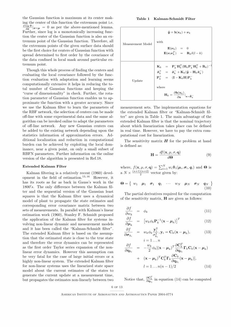
Table 1 Kalman-Schmidt Filter

Measurement Model

y = h(xk) + νk

with

E(νk) = 0

E(νlνTk ) = Rkδ(l− k)

Update

Kk = P−k HTk (HkP−k HT

k + Rk)−1

x+k = x−k + Kk(y −Hkx−k )

P+k = (I−KkH)P−k

where

Hk =∂h(xk)

∂x|x=x−k

measurement sets. The implementation equations forthe extended Kalman filter or “Kalman-Schmidt fil-ter” are given in Table 1. The main advantage of theextended Kalman filter is that the nominal trajectoryabout which linearization takes place can be definedin real time. However, we have to pay the extra com-putational cost for linearization.

The sensitivity matrix H for the problem at handis defined as:

H =df(x, µ, σ,q)

dΘ(9)

where, f(x, µ, σ,q) =∑N

i=1 wiΦi(µi, σi, qi) and Θ isa N × (n+1)(n+2)

2 vector given by:

Θ ={

w1 µ1 σ1 q1 · · · wN µN σN qN

}(10)

The partial derivatives required for the computationof the sensitivity matrix, H are given as follows:

∂f

∂wk= φk (11)

∂f

∂µk

=[wkφkP−1

k (x− µk)]T

(12)

∂f

∂σki

= wkφky2

i

σ3ki

,yi = Ck(x− µk), (13)

i = 1 . . . n∂f

∂qkl

= −wk

2φk[(x− µk)T ∂CT

k

∂qkl

ΓkCk(x− µk)

+ (x− µk)T CTk Γk

∂Ck

∂qkl

(x− µk)],

l = 1 . . . n(n− 1)/2 (14)

Notice that, ∂CTk

∂qkl

in equation (14) can be computed

6 of 13

American Institute of Aeronautics and Astronautics Paper 2004-0774

by substituting for C from equation (6):

∂Ck

∂qkl

=∂

∂qkl

(I−Qk)−1 (I + Qk)

+ (I−Qk)−1 ∂

∂qkl

(I + Qk) (15)

Making use of the fact that (I−Q)−1 (I−Q) = I, weget

∂

∂qkl

(I−Qk)−1 = (I−Qk)−1 ∂Qk

∂qkl

(I−Qk)−1

(16)substitution of equation (16) in equation (15) gives:

∂Ck

∂qkl

= (I−Qk)−1 ∂Qk

∂qkl

(I−Qk)−1 (I

+ Qk) + (I−Qk)−1 ∂Qk

∂qkl

(17)

Now equations (11)-(14) constitute the sensitivity ma-trix H for the Extended Kalman Filter. We men-tion that although equation (5) provides a minimalparametrization of the covariance matrix P, it is highlynonlinear in nature and causes problems in the con-vergence of the Kalman filter in certain cases. Toalleviate this potential difficulty and improve compu-tational speed, we present an alternate representationthe covariance matrix P known as Additive Decompo-sition.

Additive Decomposition of Covariance Matrix P

In this approach, we introduce the following param-eterization of positive definite matrices:

Additive Decomposition. Let P be a symmetricpositive definite n×n matrix then P−1 is also symmet-ric and positive definite and can be written as a sumof a diagonal matrix and a symmetric matrix:

P−1k = Γk +

n∑

i=1

n∑

j=1

eieTj qkij (18)

where ei is a n× 1 vector with only ith element equalto one and rest of them zeros and Γk is a diagonalmatrix given by:

Γk =1σ2

k

I (19)

subject to following constraints:

qkij = qkji (20)σk > 0 (21)qkii > 0 (22)

−1 ≤ qkij

(σk+qkii)(σk+qkjj

) ≤ 1 (23)

It is worthwhile to mention that qkij signifies thestretching and rotation of the Gaussian function. If

qkij= 0 then we will obtain the circular Gaussian

function.Using the additive decomposition for the Pi ma-

trix in equation (4) the different partial derivativesrequired for synthesizing the sensitivity matrix H canbe computed by defining the following parameter vec-tor Θ

Θ ={

w1 µ1 σ1 q1 · · · wN µN σN qN

}(24)

The different partial’s are then given as follows:

∂f

∂wk= φk (25)

∂f

∂µk

=[wkφkP−1

k (x− µk)]T

(26)

∂f

∂σki

= wkφk

(xi − µki)2

σ3ki

, i = 1 . . . n (27)

∂f

∂qkl

= −wkφk(xi − µki)T (xj − µkj

),

l = 1 . . . n(n + 1)\2, i, j = 1 . . . n. (28)

Thus, equations (25)-(28) constitute the sensitivitymatrix H. It is to be mentioned that even though thesynthesis of the sensitivity matrix is greatly simplified,one needs to check the constraint satisfaction definedin equations (20)-(23) at every update. In case theseconstraints are violated, we invoke the parameter pro-jection method to project the parameters back to thesets they belong to, thereby ensuring that the covari-ance matrix remains symmetric and positive definiteat all times.

The various steps for the Directed ConnectivityGraph Learning Algorithm are summarized as follows:

1. Find the interior extremum points of the givensurface-data.

2. Divide the Input space into several subspaces withthe help of equally spaced 1−D rays so that ex-tremum points do not fall on the boundary of anysubregion.

3. Find the relative maximum and minimum in eachregion.

4. Make a directed graph of all the maximum pointssorted in descending order and call it M.

5. Make a directed graph of all the minimum pointssorted in ascending order and call it N.

6. Choose first point in M and N as a candidate forGaussian center and function values as the weightof those Gaussian functions.

7. For these points find the associated covariancematrix (P) with the help of local mask.

8. Initialize qij = Pij and σ = 0.

7 of 13

American Institute of Aeronautics and Astronautics Paper 2004-0774

9. Learn w, µ, σ, qij using extended Kalman filter(Table 1) with the help of whole data.

10. Make sure that new estimated parameter vectorsatisfy the constraints given by equations (20-23)

11. Check the estimation error residuals. If they donot satisfy the required accuracy limit then choosesecond point in set M and N as Gaussian centerand follow from step 7.

Numerical Simulations and ResultsThis algorithm was tested on a variety of test func-

tions and experimental data obtained by wind tunneltesting of synthetic jet actuation wing. In this sec-tion, we will present some results from the studies,importantly a test case for function Approximationand a dynamical System identification from wind tun-nel testing of synthetic jet actuation wing.

Function Approximation

The test case for the function approximation is mo-tivated by the following analytic surface function.19

f(x1, x2) =1000

(x2 − x21)2 + (1− x1)2 + 1

+500

(x2 − 8)2 + (5− x1)2 + 1

+500

(x2 − 8)2 + (8− x1)2 + 1(29)

A random sampling of the interval [0− 10, 0− 10] forx1 and x2 is used to obtain 60 samples of each. Fig-ures 2(a) and 2(b) show the true surface and contourplots of the training set data points respectively. Ac-cording to our experience this particular function hasmany important features such as sharp ridge line thatis very difficult to learn with many existing functionapproximation algorithms with reasonable number ofnodes. The failure of these many RBFN learning algo-rithms can be attributed to the inability of the circularGaussian function to approximate a ridge kind of sur-face globally.

To approximate the function given in equation (29),we divide the whole input region into a total of 16square regions (4 in each direction). Then accordingto the procedure listed in the previous section, we gen-erate a directed connectivity graph of the local maximaand minima in each sub-region that finally add up to32 radial basis functions to have approximation errorsless than 5%. Figures 2(c) and 2(d) show the esti-mated surface and contour plots respectively. Fromthese figures, it is clear that we are able to learn theanalytical function given in equation (29) very well.Figures 2(e) and 2(f) show the error surface and errorcontour plots for the RBFN approximated function.From figure 2(e), it is clear that approximation errorsare less than 5% whereas from figure 2(f) it is clear

that even though we approximate the ramp surfacevery well most of the approximation errors are con-fined to this region alone.

SJA Modelling

In this section, the RBFN modelling results forthe synthetic jet actuator are presented. These re-sults show the effectiveness of the directed connectivitygraph learning algorithm in learning the input-outputmapping for the synthetic jet actuation wing.

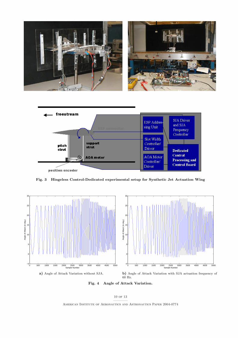
Experimental Set upA Hingeless-Control-Dedicated experimental setup

has been developed, as part of the initial effort, theheart of which is a stand-alone control unit, that con-trols all of the wing’s and SJA’s parameters and vari-ables. The setup is installed in the 3′x4′ wind tunnelof the Texas A&M Aerospace Engineering Department(Figure 3). The test wing profile for the dynamic pitchtest of the synthetic jet actuator is a NACA 0015airfoil. This shape was chosen due to the ease withwhich the wing could be manufactured and the avail-able interior space for accommodating the syntheticjet actuator (SJA).

Experimental evidence suggests that a SJA,mounted such that its jet exit tangentially to thesurface, has minimal effect on the global wing aero-dynamics at low to moderate angles of attack. Theprimary effect of the jet is at high angles of attackwhen separation is present over the upper wing sur-face. In this case, the increased mixing associated withthe action of a synthetic jet, delays or suppresses flowseparation. As such, the effect of the actuator is in thenon-linear post stall domain. To learn this nonlinearnature of SJA experiments were conducted with thecontrol-dedicated setup shown in figure 3. The wingangle of attack (AOA) is controlled by the followingreference signal.

1. Oscillation type: sinusoidal Oscillation magni-tude: 12.5◦.

2. Oscillation offset (mean AOA): 12.5◦

3. Oscillation frequency: from 0.2Hz to 20Hz.

In other words, the AOA of airfoil is forced to oscillatefrom 0◦ to 25◦ at a given frequency (see figure 4). Theexperimental data collected were the time histories ofthe pressure distribution on the wing surface (at 32locations). The data was also integrated to generatethe time histories of the lift coefficient and the pitchingmoment coefficient. Data was collected with the SJAon and with the SJA off (i.e. with and without activeflow control). All the experimental data were takenfor 5 sec at a 100 Hz sampling rate.

RBFN Modelling of Experimental DataThe experiments described above were performed

at a freestream velocity of 25m/sec. From the surface

8 of 13

American Institute of Aeronautics and Astronautics Paper 2004-0774

02

46

810

0

5

100

2

4

6

8

10

12

x1

x2

f(x,

y)

a) True Surface Plot

0 2 4 6 8 100

1

2

3

4

5

6

7

8

9

10

x1

x 2

b) True Contour Plots

02

46

810

0

5

100

2

4

6

8

10

x1

x2

f estim

ated

(x1,x

2)

c) Estimated Surface Plot

0 2 4 6 8 100

1

2

3

4

5

6

7

8

9

10

x1

x 2

d) Estimated Contour Plots

02

46

810

0

5

10−2

−1

0

1

2

x1

x2

App

roxi

mat

ion

Err

or

e) Approximation Error Surface Plot

0 2 4 6 8 100

1

2

3

4

5

6

7

8

9

10

x1

x 2

f) Approximation Error Contour Plots

Fig. 2 Simulation Results For Analytical Function given by Equation 29

9 of 13

American Institute of Aeronautics and Astronautics Paper 2004-0774

Fig. 3 Hingeless Control-Dedicated experimental setup for Synthetic Jet Actuation Wing

0 500 1000 1500 2000 2500 3000 3500 4000 4500 5000−5

0

5

10

15

20

25

30

Sample Number

Ang

le o

f Atta

ck (

in d

eg.)

a) Angle of Attack Variation without SJA.

0 500 1000 1500 2000 2500 3000 3500 4000 4500 5000−5

0

5

10

15

20

25

30

Sample Number

Ang

le o

f Atta

ck (

in d

eg.)

b) Angle of Attack Variation with SJA actuation frequency of60 Hz.

Fig. 4 Angle of Attack Variation.

10 of 13

American Institute of Aeronautics and Astronautics Paper 2004-0774

0 1000 2000 3000 4000 5000−1

−0.5

0

0.5

1

1.5

2

Sample Number

SJA

Win

g Li

ft F

orce

Desired OutputRBFN Output

a) 0 Hz jet actuation frequency.

0 1000 2000 3000 4000 5000−1

−0.5

0

0.5

1

1.5

2

Sample Number

SJA

Win

g Li

ft F

orce

Desired OutputRBFN Output

b) 60 Hz jet actuation frequency.

Fig. 5 Measured and Approximated Lift Coefficient.

0 1000 2000 3000 4000 5000−1

−0.5

0

0.5

1

1.5

2

Sample Number

App

roxi

mat

ion

Err

or

Output Error

a) 0 Hz jet actuation frequency.

0 1000 2000 3000 4000 5000−1

−0.5

0

0.5

1

1.5

2

Sample Number

App

roxi

mat

ion

Err

or

Output Error

b) 60 Hz jet actuation frequency.

Fig. 6 Approximation Error for Lift Coefficient.

0 1000 2000 3000 4000 5000−0.4

−0.3

−0.2

−0.1

0

0.1

0.2

0.3

Sample Number

Pitc

hing

Mom

ent

Desired OutputRBFN Output

a) 0 Hz jet actuation frequency.

0 1000 2000 3000 4000 5000−0.35

−0.3

−0.25

−0.2

−0.15

−0.1

−0.05

0

0.05

0.1

0.15

Sample Number

Pitc

hing

Mom

ent

Desired OutputRBFN Output

b) 60 Hz jet actuation frequency.

Fig. 7 Measured and Approximated Pitching Moment Coefficient.

11 of 13

American Institute of Aeronautics and Astronautics Paper 2004-0774

0 1000 2000 3000 4000 5000−0.4

−0.3

−0.2

−0.1

0

0.1

0.2

Sample Number

App

roxi

mat

ion

Err

or

Output Error

a) 0 Hz jet actuation frequency.

0 1000 2000 3000 4000 5000−0.2

−0.15

−0.1

−0.05

0

0.05

0.1

0.15

Sample Number

Pitc

hing

Mom

ent

Output Error

b) 60 Hz jet actuation frequency.

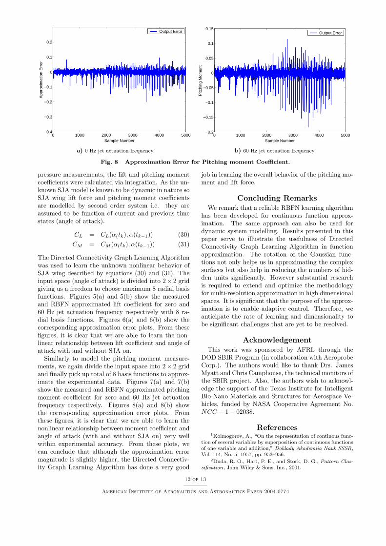
Fig. 8 Approximation Error for Pitching moment Coefficient.

pressure measurements, the lift and pitching momentcoefficients were calculated via integration. As the un-known SJA model is known to be dynamic in nature soSJA wing lift force and pitching moment coefficientsare modelled by second order system i.e. they areassumed to be function of current and previous timestates (angle of attack).

CL = CL(α(tk), α(tk−1)) (30)CM = CM (α(tk), α(tk−1)) (31)

The Directed Connectivity Graph Learning Algorithmwas used to learn the unknown nonlinear behavior ofSJA wing described by equations (30) and (31). Theinput space (angle of attack) is divided into 2× 2 gridgiving us a freedom to choose maximum 8 radial basisfunctions. Figures 5(a) and 5(b) show the measuredand RBFN approximated lift coefficient for zero and60 Hz jet actuation frequency respectively with 8 ra-dial basis functions. Figures 6(a) and 6(b) show thecorresponding approximation error plots. From thesefigures, it is clear that we are able to learn the non-linear relationship between lift coefficient and angle ofattack with and without SJA on.

Similarly to model the pitching moment measure-ments, we again divide the input space into 2× 2 gridand finally pick up total of 8 basis functions to approx-imate the experimental data. Figures 7(a) and 7(b)show the measured and RBFN approximated pitchingmoment coefficient for zero and 60 Hz jet actuationfrequency respectively. Figures 8(a) and 8(b) showthe corresponding approximation error plots. Fromthese figures, it is clear that we are able to learn thenonlinear relationship between moment coefficient andangle of attack (with and without SJA on) very wellwithin experimental accuracy. From these plots, wecan conclude that although the approximation errormagnitude is slightly higher, the Directed Connectiv-ity Graph Learning Algorithm has done a very good

job in learning the overall behavior of the pitching mo-ment and lift force.

Concluding RemarksWe remark that a reliable RBFN learning algorithm

has been developed for continuous function approx-imation. The same approach can also be used fordynamic system modelling. Results presented in thispaper serve to illustrate the usefulness of DirectedConnectivity Graph Learning Algorithm in functionapproximation. The rotation of the Gaussian func-tions not only helps us in approximating the complexsurfaces but also help in reducing the numbers of hid-den units significantly. However substantial researchis required to extend and optimize the methodologyfor multi-resolution approximation in high dimensionalspaces. It is significant that the purpose of the approx-imation is to enable adaptive control. Therefore, weanticipate the rate of learning and dimensionality tobe significant challenges that are yet to be resolved.

AcknowledgementThis work was sponsored by AFRL through the

DOD SBIR Program (in collaboration with AeroprobeCorp.). The authors would like to thank Drs. JamesMyatt and Chris Camphouse, the technical monitors ofthe SBIR project. Also, the authors wish to acknowl-edge the support of the Texas Institute for IntelligentBio-Nano Materials and Structures for Aerospace Ve-hicles, funded by NASA Cooperative Agreement No.NCC − 1− 02038.

References1Kolmogorov, A., “On the representation of continous func-

tion of several variables by superposition of continuous functionsof one variable and addition,” Doklady Akademiia Nauk SSSR,Vol. 114, No. 5, 1957, pp. 953–956.

2Duda, R. O., Hart, P. E., and Stork, D. G., Pattern Clas-sification, John Wiley & Sons, Inc., 2001.

12 of 13

American Institute of Aeronautics and Astronautics Paper 2004-0774

3Haykin, S., Neural Networks: A Comprehensive Founda-tion, Prentice Hall, 1998.

4Sundararajan, N., Saratchandran, P., Wei, L. Y., andandYingwei Lu, Y. W. L., Radial Basis Function Neural Net-works With Sequential Learning: MRAN and Its Applications,World Scientific Pub Co, December, 1999.

5Musavi, M., Ahmed, W., Chan, K., Faris, K., and Hum-mels, D., “On training of radial basis function classifiers,” Neu-ral Networks, Vol. 5, 1992, pp. 595–603.

6Tao, K., “A closer look at the radial basis function net-works,” Conference record of 27th Asilomar Conference onsignals, system and computers, Pacific Grove, CA, USA, pp.401–405.

7Poggio, T. and Girosi, F., “Networks for Approximationand learning,” Proceedings of the IEEE , Vol. 78, 1990, pp. 1481–1497.

8Moody, J. and Darken, C., “Fast learning in network oflocally-tuned processing units,” Neural Computation, Vol. 1,1989, pp. 281–294.

9S.Chen, Cowman, C., and Grant, P., “Othogonal leastsquares learning algorithm for radial basis function networks,”IEEE Transaction on Neural Networks, Vol. 2, 1991, pp. 302–309.

10Lee, S. and Kil, R., “A gaussian potential function networkwith hierarchically self-organizing learning,” Neural Networks,Vol. 4, 1991, pp. 207–224.

11Patt, J., “A resource allocating network for function inter-polation,” Neural Computation, Vol. 3.

12Kadirkamanathan, V. and Niranjan, M., “A function esti-mation approach to sequential learning with neural network,”Neural Computation, Vol. 5, 1993, pp. 954–975.

13Crassidis, J. and Junkins, J., “An introduction to OptimalEstimation of Dynamical Systems,” Unpublished book.

14Sundararajan, N., Saratchandran, P., and Li, Y., “FullyTuned Radial Basis Function Neural Networks For Flight Con-trol,” Kluwer Academic Publishers, Boston, MA, USA, 2002.

15Junkins, J. L. and Kim, Y., Introduction to Dynamics andControl of Flexible Structures, American Institute of Aeronau-tics and Astronautics, 1993.

16Singla, P., “A New Attitude Determination Approach us-ing Split Field of View Star Camera,” Masters Thesis report ,Aerospace Engineering, Texas A&M University, College Station,TX, USA.

17Boyd, S. and Vandenberghe, L., Convex Optimization,Cambridge University Press, February 2004.

18Singla, P., Griffith, T. D., Subbarao, K., and Junkins, J. L.,“Autonomous Focal Plane Calibration by an Intelligent RadialBasis Network,” AAS/AIAA Spaceflight Mechanics Conference,Mauii, Hawaii, Febrauary 2004.

19Junkins, J. L. and Jancaitis, J. R., “Smooth IrregularCurves,” Photogrammetric Engineering, June 1972, pp. 565–573.

13 of 13

American Institute of Aeronautics and Astronautics Paper 2004-0774