Page 1
i
INTELLIGENT SYSTEMS APPROACH FOR
CLASSIFICATION AND MANAGEMENT OF
PATIENTS WITH HEADACHE
by
Ahmed Jasim Mohammed Kaky (Aljaaf)
A thesis submitted in partial fulfilment of the requirements of Liverpool
John Moores University for the degree of Doctor of Philosophy
July 2017
Page 2
ii
DECLARATION
I, Ahmed Kaky, confirm that the work presented in this thesis is my own. Where
information has been derived from other sources, I confirm this has been indicated in
the thesis.
Ahmed Jasim Mohammed Kaky
Word count (Excluding acknowledgement, appendices and references): 37280 words
Page 3
iii
ACKNOWLEDGEMENT
Firstly, I would like to express my sincere gratitude to my supervisors Prof. Dr.
Dhiya Al-jumeily and Dr. Abir Hussain for the continuous support of my PhD study
and related research, for their patience, motivation, and immense knowledge. Their
guidance helped me in all the time of research and writing of this thesis. I could not
have imagined having a better supervisors and mentors for my Ph.D study.
Besides my supervisors, I wish to express my sincere thanks to Prof. Dr. Aynur
Ozge, Mersin University School of Medicine, Turkey, and her team for providing me
with the data set. I would also like to express my thanks for the inputs from Mr.
Conor Mallucci, a consultant neurosurgeon at Alder Hey hospital, Liverpool, and Mr.
Khaled Abdel-Aziz, a consultant neurologist at Ashford hospital, London. I
appreciate their help.
I take this opportunity to express my gratitude to everyone who supported me
throughout my PhD study. I appreciate the support from my family. I would
especially love to thank my wife Aysha Al-Rawi. I do not believe I can finish this
dissertation without her support. Finally, I am grateful to Allah for the good health
and wellbeing that were necessary to complete this dissertation.
Page 4
iv
ABSTRACT
Primary headache disorders are the most common complaints worldwide. The
socioeconomic and personal impact of headache disorders is enormous, as it is the
leading cause of workplace absence. Headache patients’ consultations are increasing
as the population has increased in size, live longer and many people have multiple
conditions, however, access to specialist services across the UK is currently
inequitable because the numbers of trained consultant neurologists in the UK are 10
times lower than other European countries. Additionally, more than two third of
headache cases presented to primary care were labelled with unspecified headache.
Therefore, an alternative pathway to diagnose and manage patients with primary
headache could be crucial to reducing the need for specialist assessment and increase
capacity within the current service model. Several recent studies have targeted this
issue through the development of clinical decision support systems, which can help
non-specialist doctors and general practitioners to diagnose patients with primary
headache disorders in primary clinics. However, the majority of these studies were
following a rule-based system style, in which the rules were summarised and
expressed by a computer engineer. This style carries many downsides, and we will
discuss them later on in this dissertation.
In this study, we are adopting a completely different approach. The use of machine
learning is recruited for the classification of primary headache disorders, for which a
dataset of 832 records of patients with primary headaches was considered,
originating from three medical centres located in Turkey. Three main types of
primary headaches were derived from the data set including Tension Type Headache
in both episodic and chronic forms, Migraine with and without Aura, followed by
Trigeminal Autonomic Cephalalgia that further subdivided into Cluster headache,
paroxysmal hemicrania and short-lasting unilateral neuralgiform headache attacks
with conjunctival injection and tearing. Six popular machine-learning based
classifiers, including linear and non-linear ensemble learning, in addition to one
regression based procedure, have been evaluated for the classification of primary
headaches within a supervised learning setting, achieving highest aggregate
performance outcomes of AUC 0.923, sensitivity 0.897, and overall classification
accuracy of 0.843.
Page 5
v
This study also introduces the proposed HydroApp system, which is an M-health
based personalised application for the follow-up of patients with long-term
conditions such as chronic headache and hydrocephalus. We managed to develop this
system with the supervision of headache specialists at Ashford hospital, London, and
neurology experts at Walton Centre and Alder Hey hospital Liverpool. We have
successfully investigated the acceptance of using such an M-health based system via
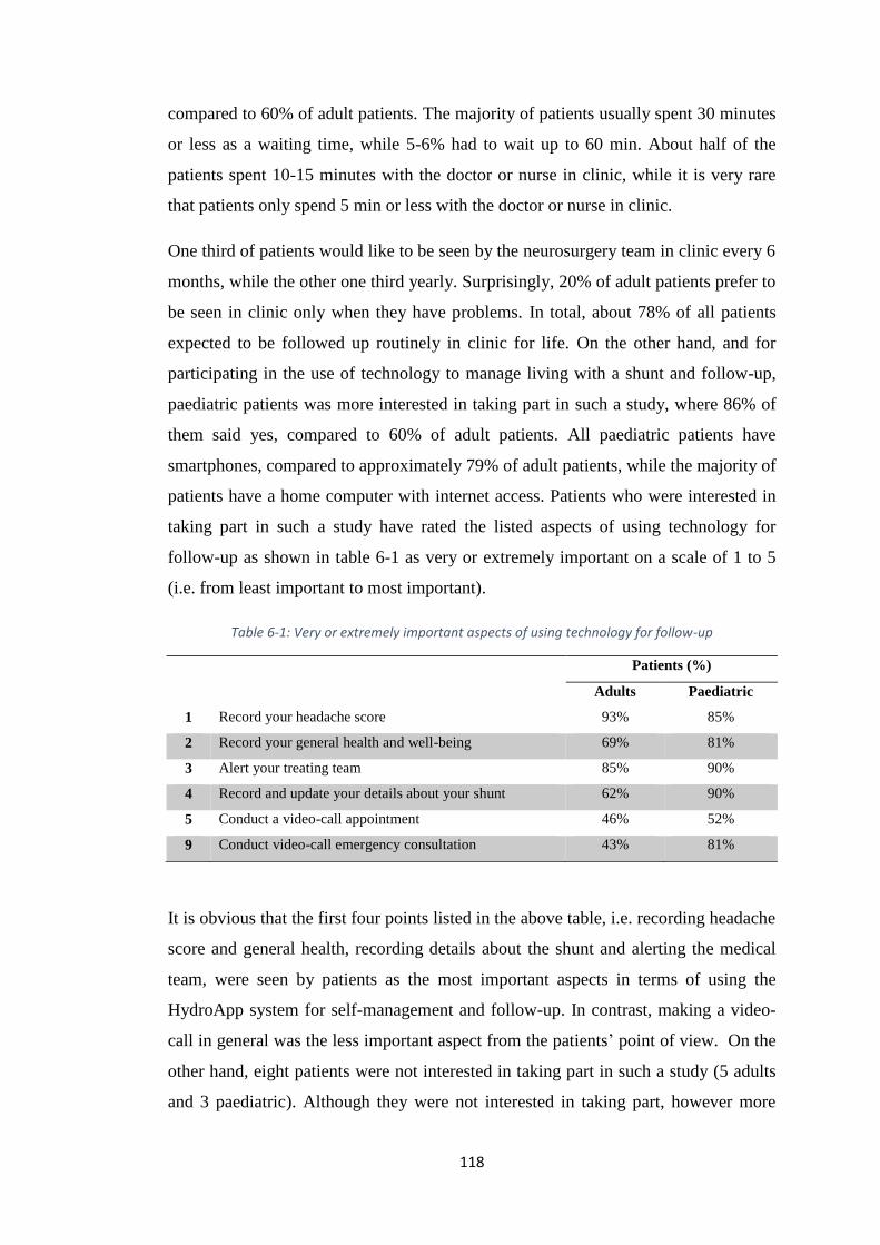
an online questionnaire, where 86% of paediatric patients and 60% of adult patients
were interested in using HydroApp system to manage their conditions. Features and
functions offered by HydroApp system such as recording headache score, recording
of general health and well-being as well as alerting the treating team, have been
perceived as very or extremely important aspects from patients’ point of view.
The study concludes that the advances in intelligent systems and M-health
applications represent a promising atmosphere through which to identify alternative
solutions, which in turn increases the capacity in the current service model and
improves diagnostic capability in the primary headache domain and beyond.
Page 6
vi
TABLE OF CONTENTS
ACKNOWLEDGEMENT .......................................................................................... vi
ABSTRACT ............................................................................................................... ivi
TABLE OF CONTENTS ........................................................................................... vi
LIST OF FIGURES ................................................................................................... ix
LIST OF TABLES ...................................................................................................... x
ABBREVIATIONS .................................................................................................... xi
Chapter 1: INTRODUCTION ............................................................................ 1
1.1. Overview .................................................................................................... 1
1.2. Problem statement...................................................................................... 2
1.3. Research question ...................................................................................... 3
1.4. Research aims and objectives .................................................................... 3
1.5. Research scope ........................................................................................... 6
1.6. Research contributions ............................................................................... 6
1.7. Structure of the thesis ................................................................................ 7
Chapter 2: HEADACHE DISORDERS ............................................................. 9
2.1. Introduction ................................................................................................ 9
2.2. Types of headaches .................................................................................... 9
2.3. Primary headache disorders ..................................................................... 12
2.3.1. Migraine ........................................................................................... 12
2.3.2. Tension-type headache ..................................................................... 14
2.3.3. Trigeminal Autonomic Cephalalgias (TACs) .................................. 16
3.3.3.1 Cluster headache .............................................................................. 16
3.3.3.2 Paroxysmal hemicrania ................................................................... 18
3.3.3.3 SUNCT ............................................................................................ 18
2.4. Presentation and comparison ................................................................... 19
2.5. Secondary headache disorders ................................................................. 21
2.6. Chapter summary ..................................................................................... 22
Chapter 3: LITERATURE REVIEW .............................................................. 23
3.1. Introduction .............................................................................................. 23
3.2. Intelligent driven modules to diagnose headaches .................................. 23
Page 7
vii
3.2.1. Neurologist expert system (NES) ..................................................... 24
3.2.2. Expert system based headache solution (ESHS) .............................. 24
3.2.3. A guideline-based DSS for headache diagnosis ............................... 25
3.2.4. Validation of a guideline-based DSS for headache diagnosis .......... 25
3.2.5. Case-based reasoning DSS for headache diagnosis ......................... 25
3.2.6. Hybrid intelligent reasoning DSS ..................................................... 26
3.2.7. Automatic DSS for the classification of primary headaches ............ 26
3.2.8. Other headache diagnostic modules ................................................. 27
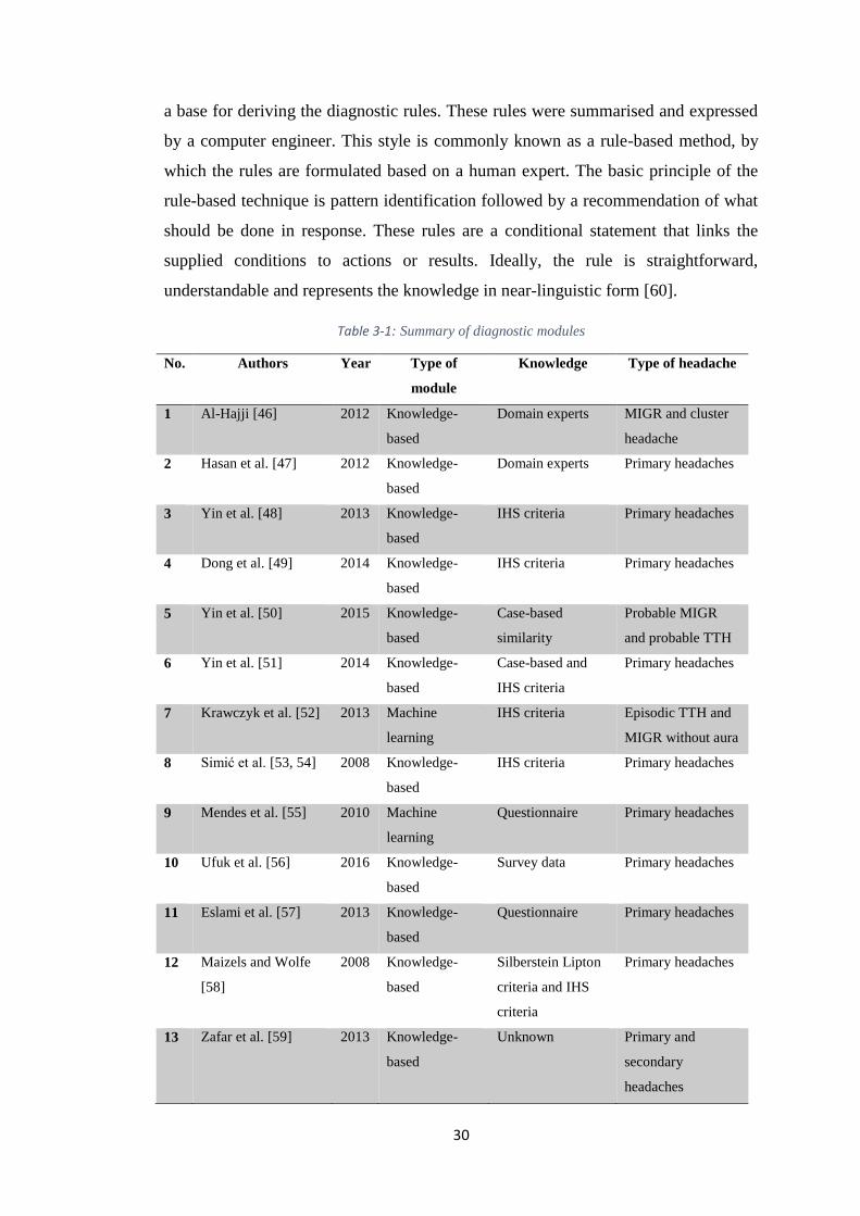
3.3. Evaluation and justifications .................................................................... 28
3.4. Chapter summary ..................................................................................... 31
Chapter 4: DATA PREPARATION ................................................................ 33
4.1. Introduction .............................................................................................. 33
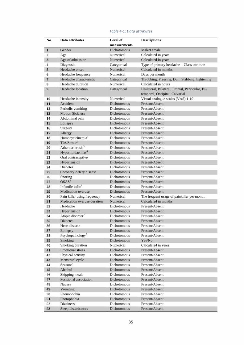
4.2. Data description ....................................................................................... 33
4.3. Outliers’ detection.................................................................................... 37
4.4. Missing Data ............................................................................................ 42
4.4.1. Missing data mechanism .................................................................. 42
4.4.2. Processing of missing data ............................................................... 47
4.4.3. Multiple imputations ........................................................................ 50
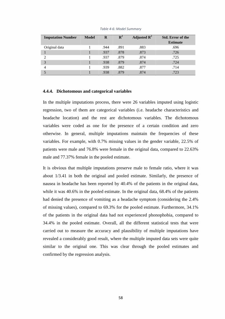
4.4.4. Dichotomous and categorical variables ............................................ 58
4.5. Data normalisation ................................................................................... 59
4.6. Chapter summary ..................................................................................... 60
Chapter 5: PREDICTIVE MODELS ............................................................... 61
5.1. Introduction .............................................................................................. 61
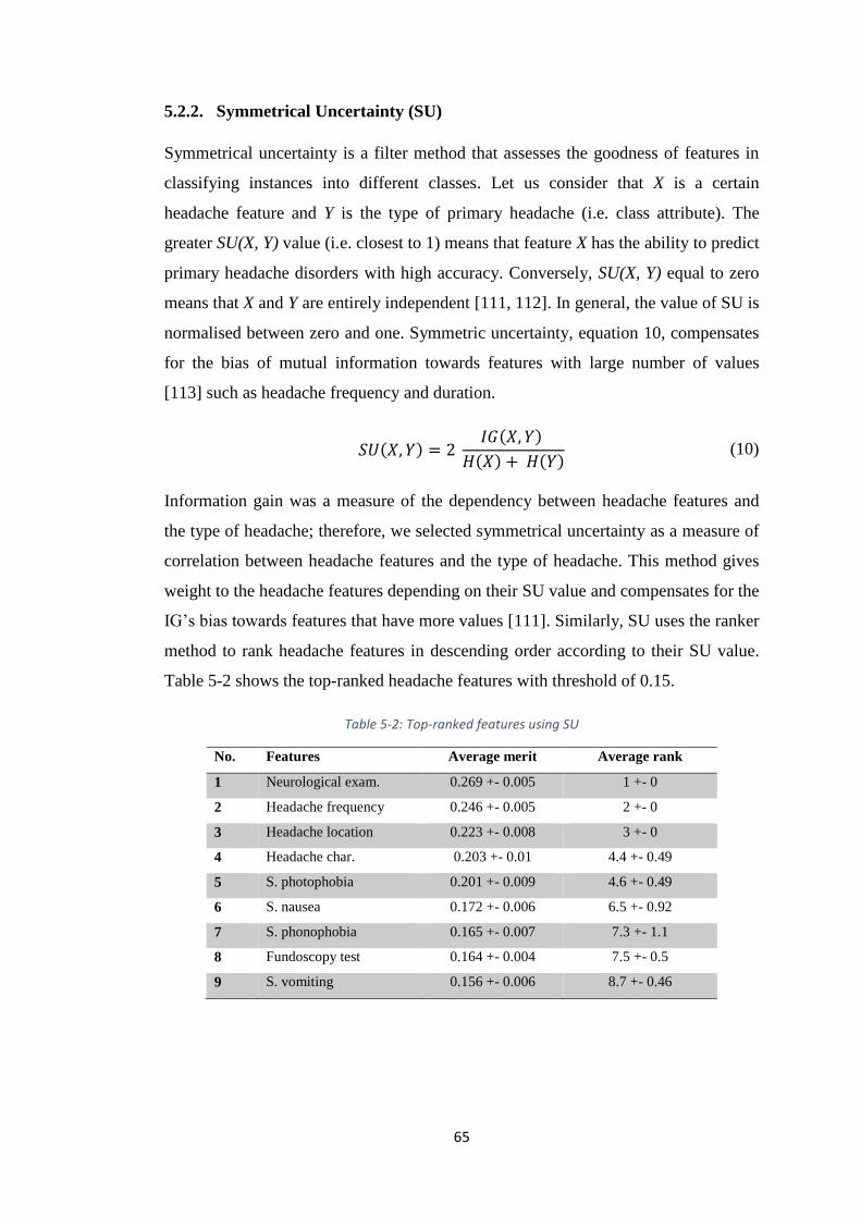
5.2. Feature selection ...................................................................................... 61
5.2.1. Information gain (IG) ....................................................................... 63
5.2.2. Symmetrical Uncertainty (SU) ......................................................... 65
5.2.3. Multilayer perceptron (MLP) ........................................................... 66
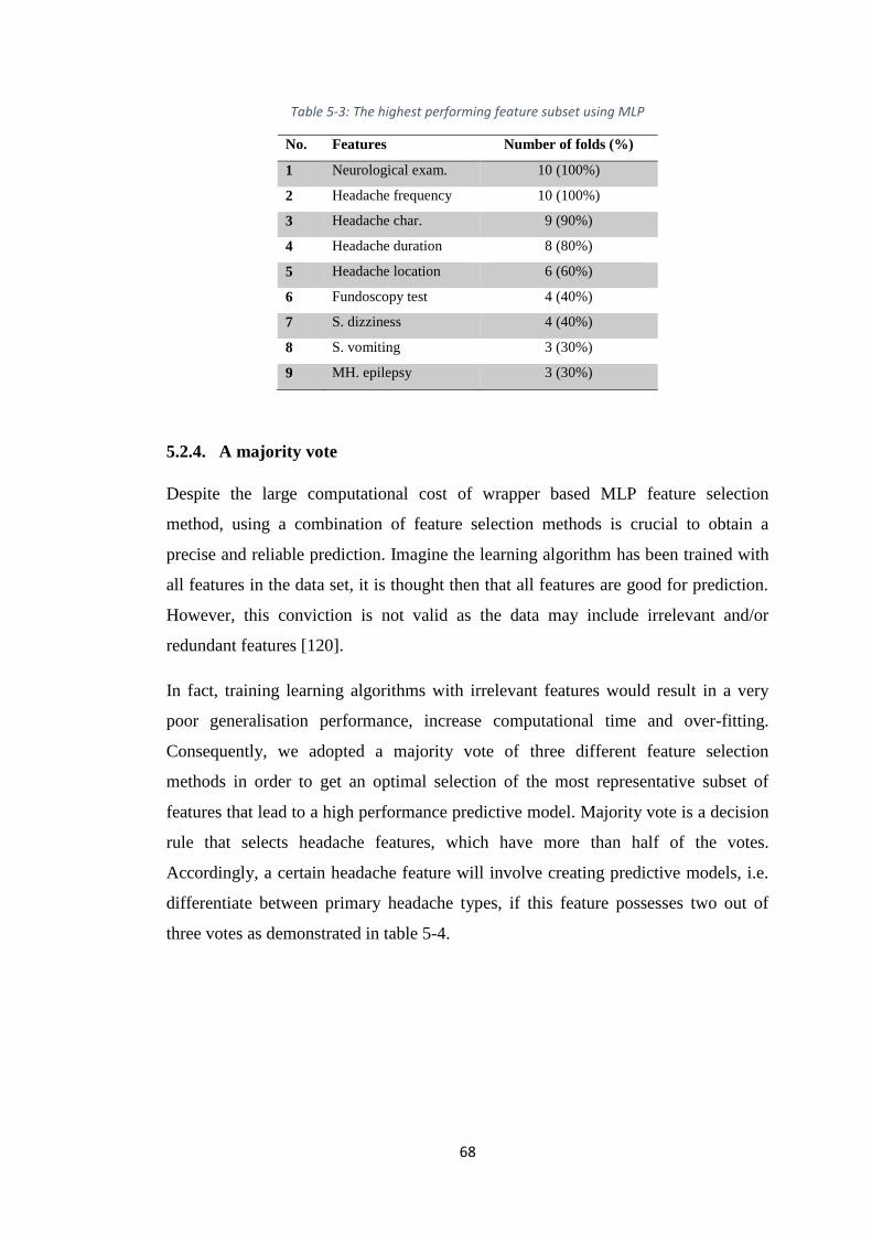
5.2.4. A majority vote ................................................................................. 68
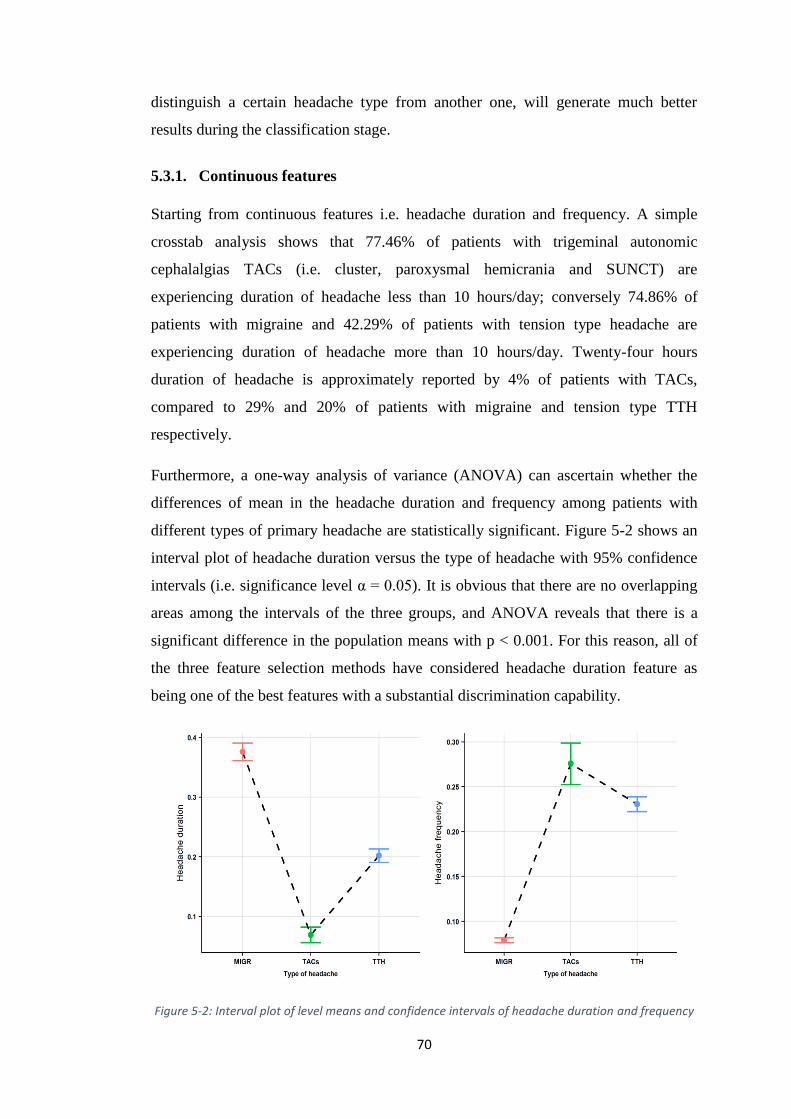
5.3. Feature analysis........................................................................................ 69
5.3.1. Continuous features .......................................................................... 70
5.3.2. Discrete features ............................................................................... 71
5.3.2.1 Headache characteristic ................................................................... 72
5.3.2.2 Headache location ........................................................................... 73
Page 8
viii
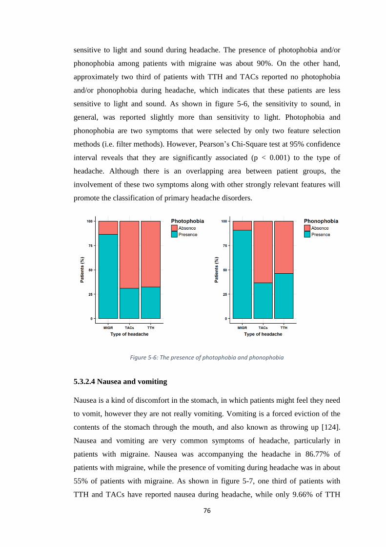
5.3.2.3 Photophobia and phonophobia ........................................................ 75
5.3.2.4 Nausea and vomiting ....................................................................... 76
5.3.2.5 Neurological examination and Fundoscopy test ............................. 77
5.3.3. Summary of analysis ........................................................................ 80
5.4. Class balancing and Binarization ............................................................. 83
5.5. Performance metrics ................................................................................ 85
5.6. Predictive models ..................................................................................... 87
5.6.1. Tension type headache vs. all ........................................................... 88
5.6.2. Migraine vs. all ................................................................................. 90
5.6.3. TACs vs. all ...................................................................................... 90
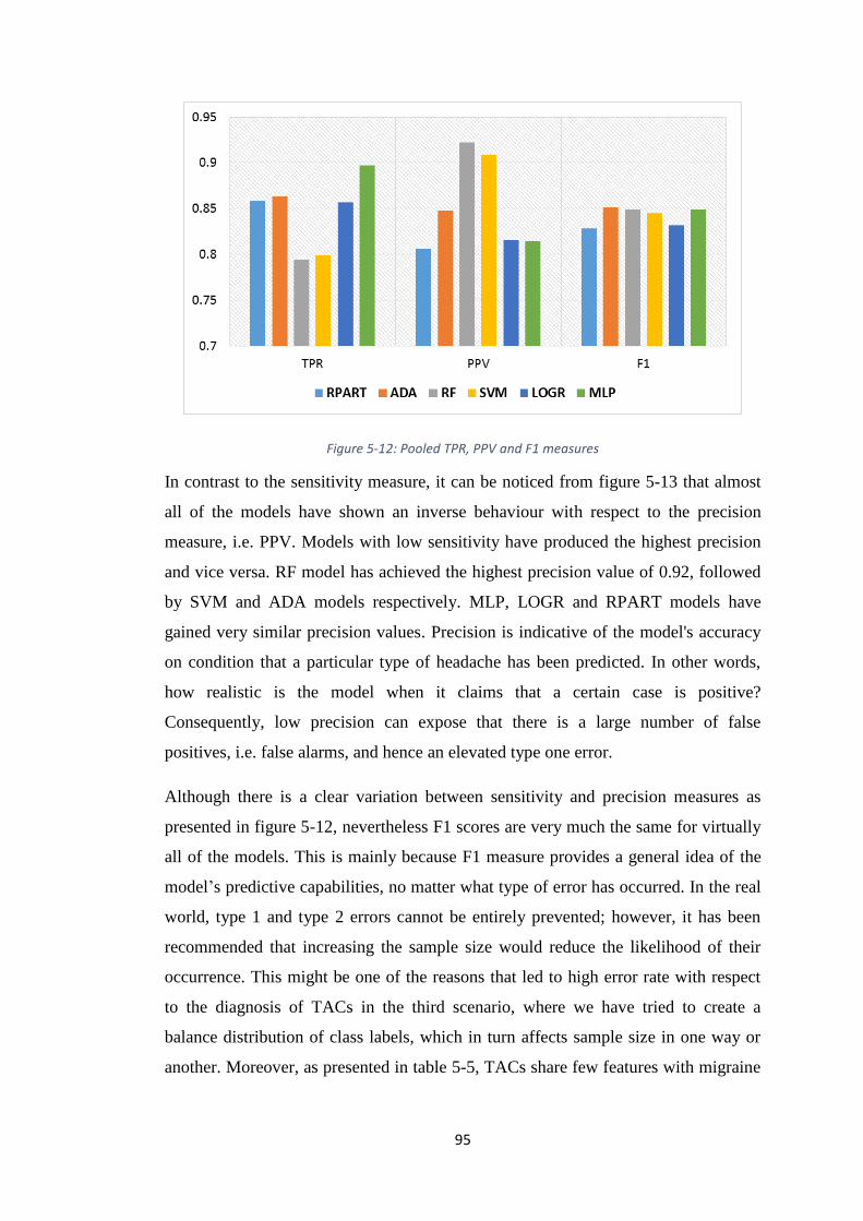
5.7. Pooling and discussion............................................................................. 91
5.8. Chapter summary ................................................................................... 103
Chapter 6: HEADACHE FOLLOW-UP ....................................................... 104
6.1. Introduction ............................................................................................ 104
6.2. The HydroApp system ........................................................................... 104
6.3. HydroApp system architecture .............................................................. 105
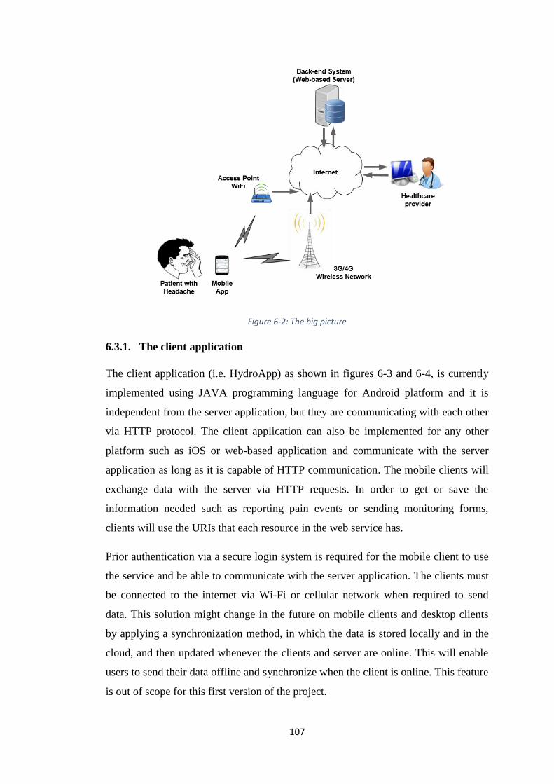
6.3.1. The client application ..................................................................... 107
6.3.2. The server application .................................................................... 109
6.3.3. Central database ............................................................................. 110
6.3.4. Data privacy and security ............................................................... 112
6.3.5. Authentication and authorisation .................................................... 113
6.3.6. Application usability ...................................................................... 115
6.4. HydroApp system in use for clinical follow-up study ........................... 115
6.5. The benefits of HydroApp system ......................................................... 119
6.6. Chapter summary ................................................................................... 121
Chapter 7: CONCLUSION AND FUTURE WORK .................................... 122
7.1. Conclusion ............................................................................................. 122
7.2. Future work ............................................................................................ 124
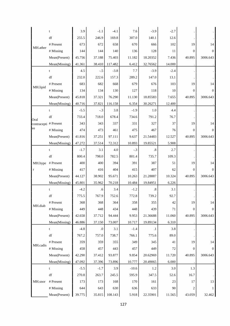
Appendix A: Separate Variance t Tests .................................................................. 125
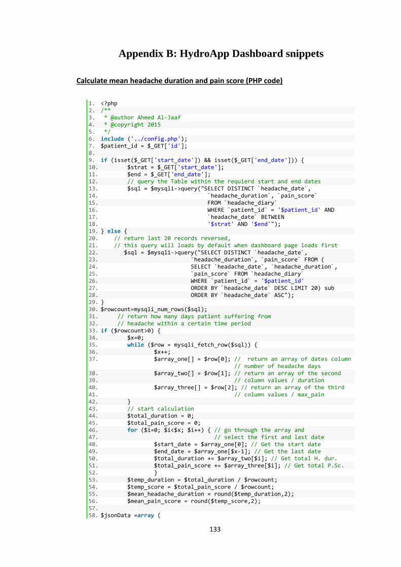
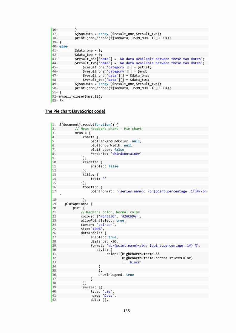
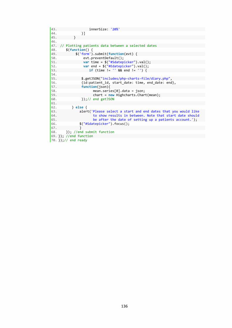
Appendix B: HydroApp Dashboard snippets ......................................................... 133
Appendix C: List of publications ............................................................................ 137
REFERENCES ....................................................................................................... 139
Page 9
ix
LIST OF FIGURES FIGURE 1-1: RESEARCH MAP ......................................................................................... 5
FIGURE 2-1: TYPES OF HEADACHE ............................................................................... 10
FIGURE 3-1: TYPES OF CLINICAL DECISION SUPPORT SYSTEMS .................................... 29
FIGURE 4-1: DATA OUTLIERS ...................................................................................... 39
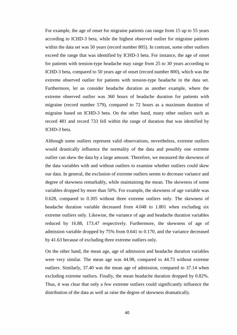
FIGURE 4-2: DATA WITHOUT OUTLIERS ....................................................................... 41
FIGURE 4-3: OVERALL SUMMARY OF MISSING DATA ................................................... 44
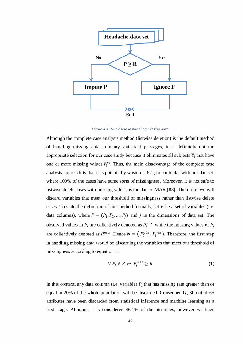
FIGURE 4-4: OUR VISION IN HANDLING MISSING DATA ................................................ 49
FIGURE 5-1: A TYPICAL MLP NEURAL NETWORK ....................................................... 66
FIGURE 5-2: INTERVAL PLOT OF LEVEL MEANS AND CONFIDENCE INTERVALS OF
HEADACHE DURATION AND FREQUENCY .............................................................. 70
FIGURE 5-3: HOW HEADACHE PATIENTS DESCRIBE THEIR PAIN ................................... 73
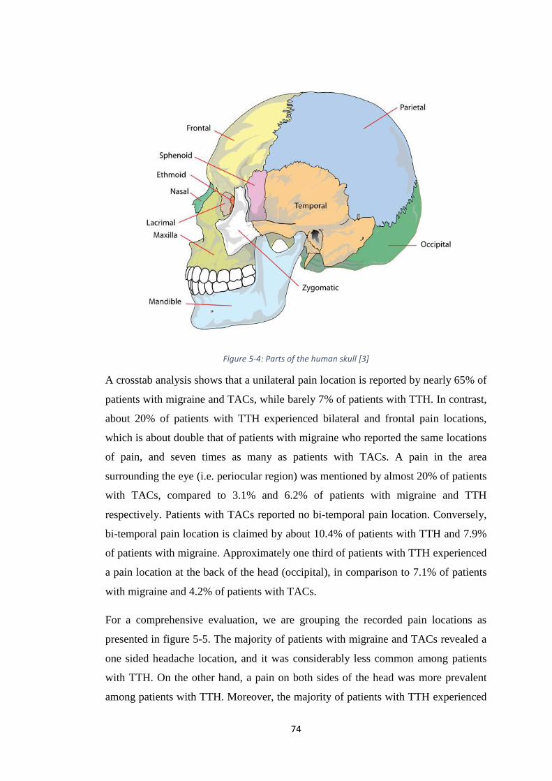
FIGURE 5-4: PARTS OF THE HUMAN SKULL [3] ............................................................ 74
FIGURE 5-5: GROUPING THE LOCATIONS OF PAIN ........................................................ 75
FIGURE 5-6: THE PRESENCE OF PHOTOPHOBIA AND PHONOPHOBIA ............................. 76
FIGURE 5-7: THE PRESENCE OF NAUSEA AND VOMITING .............................................. 77
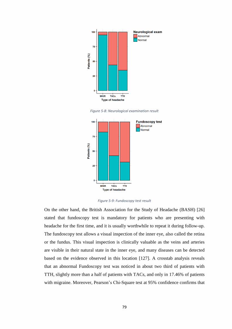
FIGURE 5-8: NEUROLOGICAL EXAMINATION RESULT .................................................. 79
FIGURE 5-9: FUNDUSCOPIC TEST RESULT .................................................................... 79
FIGURE 5-10: PERFORMANCE OF MLS (TTH VS. ALL) ................................................ 89
FIGURE 5-11: ROC PLOTS FOR THE MODELS ............................................................... 93
FIGURE 5-12: POOLED TPR, PPV AND F1 MEASURES ................................................. 95
FIGURE 5-13: POOLED ACC AND AUC ....................................................................... 96
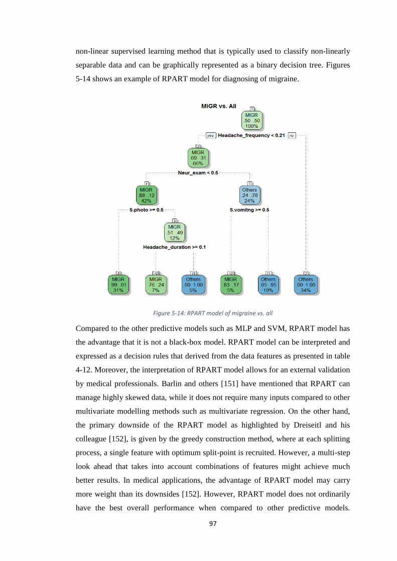
FIGURE 5-14: RPART MODEL OF MIGRAINE VS. ALL ................................................... 97
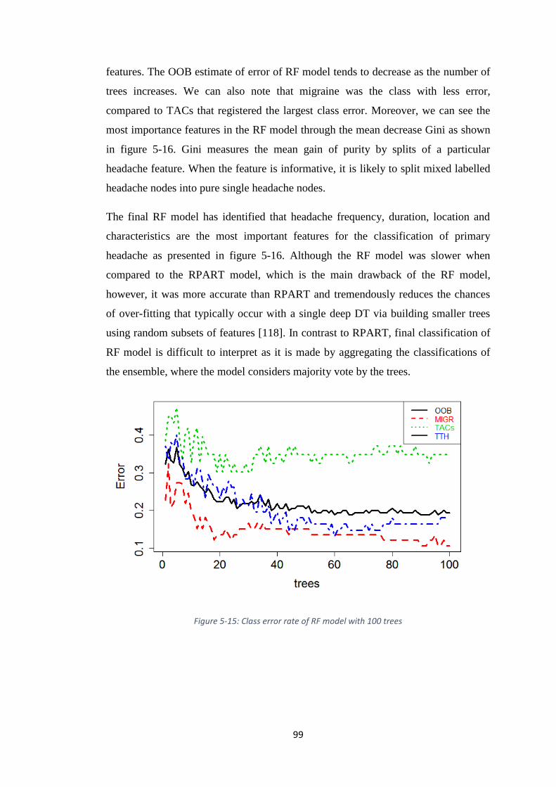
FIGURE 5-15: CLASS ERROR RATE OF RF MODEL WITH 100 TREES .............................. 99
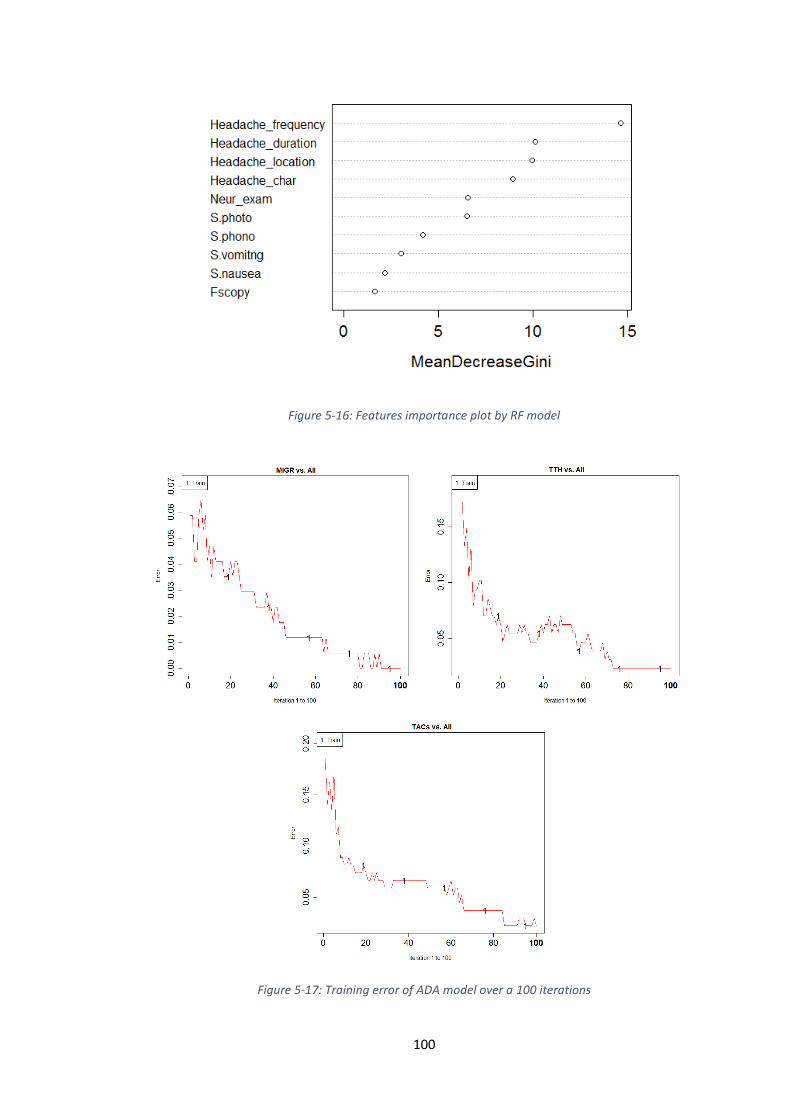
FIGURE 5-16: FEATURES IMPORTANCE PLOT BY RF MODEL ...................................... 100
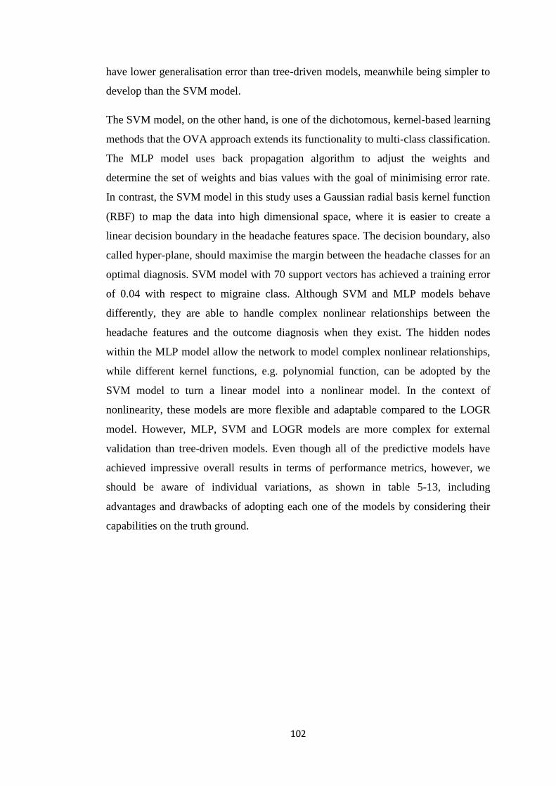
FIGURE 5-17: TRAINING ERROR OF ADA MODEL OVER A 100 ITERATIONS ................ 100
FIGURE 6-1: SIMPLE OVERVIEW OF 3-TIER APPLICATIONS ......................................... 106
FIGURE 6-2: THE BIG PICTURE ................................................................................... 107
FIGURE 6-3: HYDROAPP SCREENSHOTS 1 .................................................................. 108
FIGURE 6-4: HYDROAPP SCREENSHOTS 2 .................................................................. 108
FIGURE 6-5: EXAMPLE OF PATIENTS PROFILES .......................................................... 109
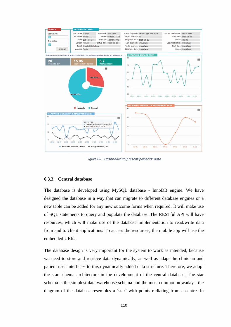
FIGURE 6-6: DASHBOARD TO PRESENT PATIENTS’ DATA ........................................... 110
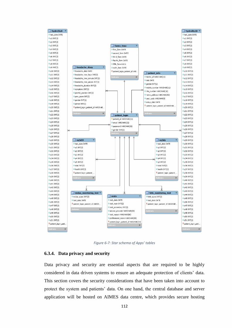
FIGURE 6-7: STAR SCHEMA OF APPS’ TABLES ........................................................... 112
FIGURE 6-9: AUTHENTICATION PROCESS ................................................................... 114
Page 10
x
LIST OF TABLES TABLE 2-1: THE DIFFERENCE BETWEEN THE PRIMARY AND SECONDARY HEADACHE .. 11
TABLE 2-2: MIGRAINE WITHOUT AURA ....................................................................... 13
TABLE 2-3: MIGRAINE WITH TYPICAL AURA ............................................................... 14
TABLE 2-4: TENSION-TYPE HEADACHE ....................................................................... 16
TABLE 2-5: CLUSTER HEADACHE ................................................................................ 17
TABLE 2-6: COMPARISON OF MIGRAINE, TENSION-TYPE AND TACS ........................... 20
TABLE 3-1: SUMMARY OF DIAGNOSTIC MODULES ....................................................... 30
TABLE 4-1: DATA ATTRIBUTES ................................................................................... 35
TABLE 4-2: VARIABLE SUMMARY A,B
.......................................................................... 45
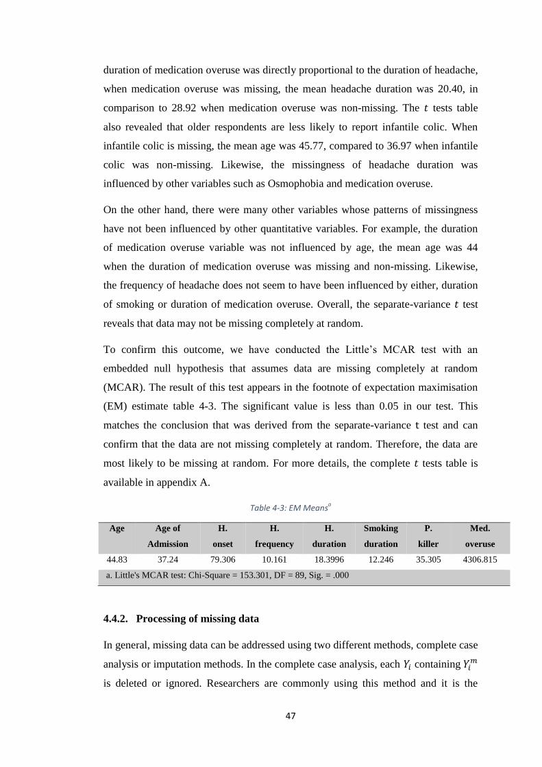
TABLE 4-3: EM MEANSA ............................................................................................. 47
TABLE 4-4: IMPUTATION MODELS .............................................................................. 53
TABLE 4-5: STATISTICS FOR MI .................................................................................. 56
TABLE 4-6: MODEL SUMMARY ................................................................................... 58
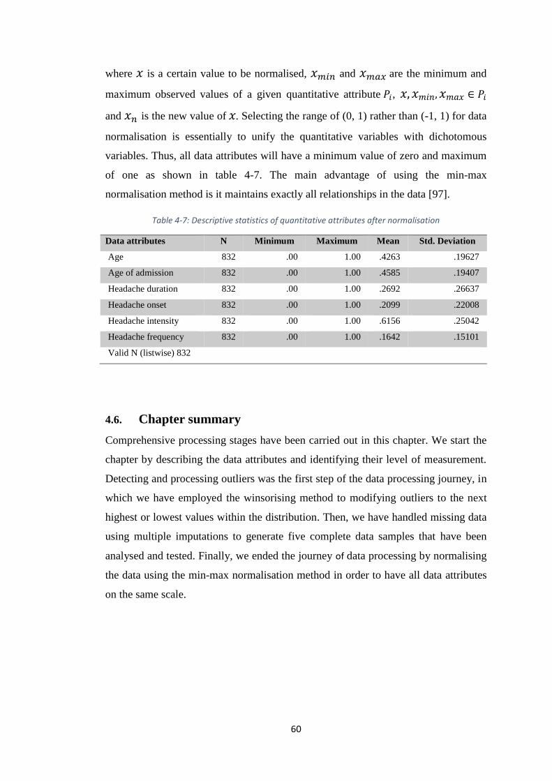
TABLE 4-7: DESCRIPTIVE STATISTICS OF QUANTITATIVE ATTRIBUTES AFTER
NORMALISATION .................................................................................................. 60
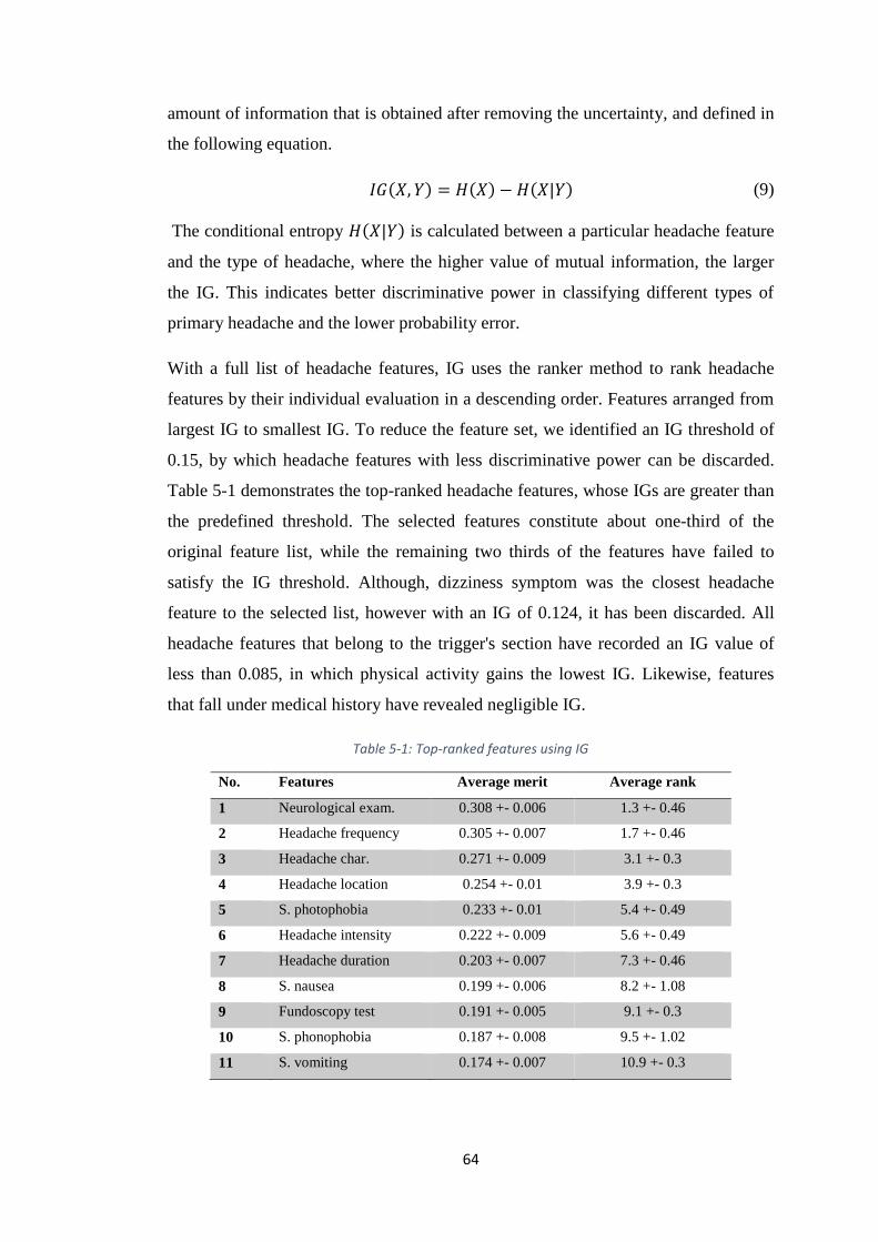
TABLE 5-1: TOP-RANKED FEATURES USING IG ............................................................ 64
TABLE 5-2: TOP-RANKED FEATURES USING SU ........................................................... 65
TABLE 5-3: THE HIGHEST PERFORMING FEATURE SUBSET USING MLP ........................ 68
TABLE 5-4: FEATURES EVALUATION (ALL FEATURES ARE CONSIDERED) ..................... 69
TABLE 5-5: SELECTED FEATURES EVALUATION........................................................... 81
TABLE 5-6: CONFUSION MATRIX ................................................................................. 86
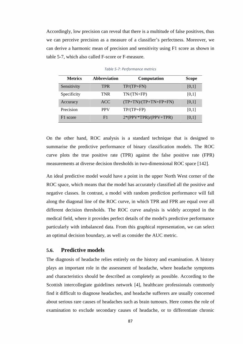
TABLE 5-7: PERFORMANCE METRICS ........................................................................... 87
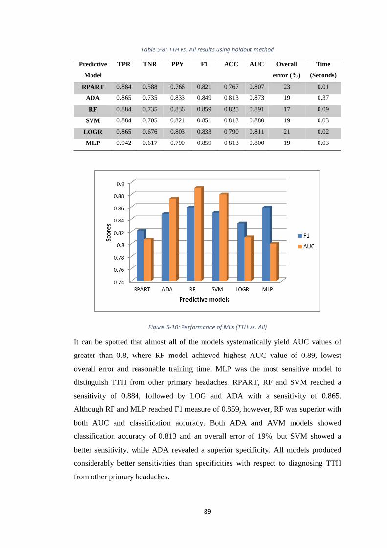
TABLE 5-8: TTH VS. ALL RESULTS USING HOLDOUT METHOD .................................... 89
TABLE 5-9: MIGR VS. ALL RESULTS USING HOLDOUT METHOD .................................. 90
TABLE 5-10: TACS VS. ALL RESULTS USING HOLDOUT METHOD ................................ 91
TABLE 5-11: POOLED RESULTS.................................................................................... 94
TABLE 5-12: THE TRANSLATION OF FIGURE 4-16 INTO A SET OF RULES ....................... 98
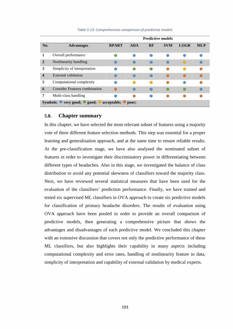
TABLE 5-13: COMPREHENSIVE COMPARISON OF PREDICTIVE MODELS ...................... 103
TABLE 6-1: VERY OR EXTREMELY IMPORTANT ASPECTS OF USING TECHNOLOGY FOR
FOLLOW-UP ........................................................................................................ 118
Page 11
xi
ABBREVIATIONS
GPs General Practitioners
NHS UK’s National Health Service
WHO World Health Organisation
IHS International Headache Society
ICHD International Classification of Headache Disorders
AMPP American Migraine Prevalence and Prevention
SIGN Scottish Intercollegiate Guidelines Network
BASH The British Association for the Study of Headache
NICE National Institute For Health and Clinical Excellence
BASICS The British Antibiotic and Silver Impregnated
Catheters for VP Shunts
VPS Ventriculoperitoneal Shunts
Hydro-OQ Hydrocephalus Outcome Questioner
PRO Patient Reported Outcome
RCT Randomised Control Trial
SWAT Study Within a Trial
HIT-6 Headache Impact Test
MIDAS Migraine Disability Assessment Test
MIGR Migraine
CM Chronic Migraine
EM Episodic Migraine
MwA Migraine with Aura
MwoA Migraine without Aura
TTH Tension-type Headache
TACs Trigeminal Autonomic Cephalalgias
CH Cluster Headache
PH Paroxysmal Hemicrania
SUNCT Short-lasting Unilateral Neuralgiform headache attacks
with Conjunctival injection and Tearing
OSAS Obstructive Sleep Apnoea syndrome
TrPs Trigger Points
FHP Forward Head Posture
M-health Mobile health
e-health Electronic health
DSS Decision Support Systems
ML Machine Learning
CBR Case-Based Reasoning
RBFL Rule-based Fuzzy Logic
RPART Classification and Regression Tree
ADA Adaptive Boosting
Page 12
xii
RF Random Forest
SVM Support Vector Machine
LOGR Logistic Regression
LINR Liner regression
MLP Multilayer perceptron
GA Genetic Algorithm
KNN K-Nearest Neighbour
IQR Interquartile Range
MCAR Missing Completely at Random
MAR Missing at Random
NMAR Not Missing at Random
EM Expectation Maximisation
FCS Fully Conditional Specification
MI Multiple Imputations
MEL Maximum Likelihood Estimation
MCMC Markov Chain Monte Carlo
LOCF Last Observation Carried Forward
IG Information Gain
SU Symmetrical Uncertainty
ANOVA Analysis Of Variance
OVA One Versus All
ROC Receiver Operating Curve
AUC Area Under The ROC Curve
PPV Positive Predictive Value
TPR True Positive Rate
FPR False Positive Rate
FNR False Negative Rate
CP Complexity Parameter
OOB Out-Of-Bag error
Page 13
1
CHAPTER 1: INTRODUCTION
1.1. Overview
Headache is the commonest neurological symptom presenting to general
practitioners (GPs) and neurologists. It can be a symptom of many different diseases
and disorders, with a variety of forms, frequency and severity from mild that
disappear easily, to severe and repeated disabling headache that can be painful and
debilitating in some individuals [1, 2]. Since 1988, The International Headache
Society (IHS) has established a standardised terminology and consistent operational
diagnostic criteria for a wide range of headaches under the term of International
Classification of Headache Disorders [3]. These criteria are derived according to an
international consensus of headache experts and have been accepted as a gold
standard for headache diagnosis. The current revision of IHS criteria, i.e. ICHD-3
beta was published in 2013.
Headaches, according to IHS criteria, are broadly classified into primary and
secondary. Primary headaches, such as migraine (MIGR), tension-type headache
(TTH) and trigeminal autonomic cephalalgias (TACs), are the most common in the
community and they are not related to any underlying medical condition, where the
headache itself is the disorder [3-5]. While secondary headache disorders occur
secondarily to another medical condition, some of which may be life threatening and
therefore require quick and accurate diagnosis. Secondary headache is extremely rare
and represents less than 1% of the population who experience headaches [6, 7].
In the UK, the lifetime prevalence of headaches is 90% of the general population [4],
and the annual headache consultation is 4.4% of all primary care consultations [6].
The personal, social and economic burden of headache disorders is enormous.
Migraine is classed by the World Health Organisation (WHO) as one of the 20
leading causes of disability amongst adults [8]. There are an estimated 6.7 million
people living with migraine in England [9], and around 83,000 people miss work or
school every day, because of headache, which is equivalent to 20 million days of lost
productivity per year [10], with a cost to the UK economy that may exceed 1.5
billion pound a year [11].
Page 14
2
1.2. Problem statement
Patients with headaches usually do not seek medical help from their GPs until the
headache really affects their quality of life, and when they do seek medical help, the
diagnosis is usually incorrect and the condition improperly managed. This was
clearly shown by a UK study of the primary care database, which revealed that 70%
of headaches were not assigned a diagnostic label [6]. Another similar study
conducted in the USA revealed that 69% of headache sufferers were labelled with
unspecified headache in the primary care [12]. The findings of these two studies
made clear that GPs encounter difficulty in the diagnosis of headaches, which in turn
may increase the pressure on the specialist neurology clinics.
Headache referrals currently account for around a third of outpatient referrals to
specialist neurology clinics across the UK [7, 13]. However, access to specialist
services across the country is currently inequitable. This is due to the fact that the
numbers of trained consultant neurologists in the UK are 10 times lower than other
European countries [11], and this problem is exacerbated further by the inequitable
distribution of specialist headache clinics between regions in England [14].
Patients with chronic headache are usually asked to fill in headache diaries or
outcome measures such as Headache Impact Test (HIT-6) and Migraine Disability
Assessment Test (MIDAS) on a regular basis; specialists use these forms to measure
the impact of headache on a patient’s life. However, within publicly funded health
care systems such as the UK’s National Health Service (NHS), long term monitoring
in neurology clinics or GPs appears not to be possible for all patients with chronic
headache due to the continued decline in funding over the past decade. This was
shown by a study conducted in 2016, which revealed that more patients in Britain
will be unable to obtain an appointment with their GPs due to the decline in GPs
funding by 17% of the NHS budget [15].
Accordingly, an alternative pathway to diagnose and manage patients with headache
is necessary to improve patient care as well as to conquer the challenges facing the
NHS. This is what Hedley Emsley, a consultant neurologist at the Department of
Neurology, Royal Preston Hospital, has confirmed in his online article for the Health
service journal (HSJ) [13]. Therefore, this study proposes an intelligent solution to
overcome these difficulties via two main points. First, the use of Machine Learning
Page 15
3
(ML) to improve the diagnosis of primary headaches, in which a set of ML classifiers
will be used to build several diagnostic or predictive models from a real-world
dataset of patients with primary headaches. The second point is adopting mobile
health (M-health) technology to provide an effective platform for long-term patient
follow-up. This study aims to contribute to this gap in knowledge.
ML classifiers can learn and gain knowledge from previous experiences and/or
through identifying patterns in medical data. They are able to learn the important
features of a given dataset, i.e. primary headaches that are diagnosed by specialists,
in order to make predictions about other data, i.e. new headache cases, which were
not a part of the original training set. The ML based diagnostic model will act as a
decision support to assist non-specialist doctors or nurses in GPs’ surgeries to make
accurate diagnosis with respect to patients with primary headaches. This in turn
could reduce the need for specialist assessment and thus referrals to neurology
clinics.
Likewise, M-health application represents an intelligent solution, and holds potential
to allow specialists to monitor a larger number of patients with chronic headache
than would be possible within the current service model. It could replace traditional
paper based headache diaries and outcome measures and provide several advantages
including improved monitoring of historical responses to therapies, improved
recording of side effects and it can be adapted to improve communication between
patients and clinicians. A remote follow-up using M-health technology can promote
the quality of care given to this category of patients as well as engaging them in their
condition management. Therefore, our proposed pathway is a great step toward
optimal patient care and proper clinical management.
1.3. Research question
Is it possible to use machine-learning methods supported by M-health technology for
diagnosing and follow-up of patients with headache?
1.4. Research aims and objectives
The main aim of this study is to provide a robust and effective diagnostic support
model to improve the diagnosis or classification of primary headache disorders using
ML methods, and initialising a user-friendly central control platform that would
Page 16
4
support and facilitate the headache specialist's task and increase their productivity
with respect to long-term follow-up and clinical management of patients with
headache. We will work towards these aims by addressing the following objectives
and as shown in the research map (Figure 1-1).
1. Review and comprehend primary headache disorders in accordance with the
latest clinical guidelines, in addition to initialising an overall comparison
among their types.
2. Review and evaluate various research studies and intelligent decision support
systems (DSS) that aimed at improving the classification or the diagnosis of
primary headache disorders. These studies or systems are going to be
assessed and compared against each other in order to identify their points of
strength and weakness and examine their intelligent module as well as the
overall efficiency and outcomes.
3. Prepare for a data acquisition procedure. This is probably the most
challenging part of the study, which requires establishing links or getting in
contact with dozens of research groups, specialised headache centres and
hospitals as well as headache associations such as the British Association for
the Study of Headache.
4. Design the data quality framework to the highest possible standard. This
framework outlines and describes almost all of the essential measures for data
processing and analysis, making use of the most advanced and sophisticated
computational and statistical approaches. This step helps to ensure that the
data is clean enough, legitimate and the ML classifiers can use the most
relevant features.
5. Develop and evaluate several diagnostic or predictive models using a number
of ML classifiers trained with data records of patients with primary
headaches. These intelligent predictive models are going to be assessed using
different performance matrices as a way to demonstrate their discriminatory
power. An overall comparison can bring about the best performing predictive
model.
6. Design and develop an M-health based application along with a central
control system prototype to enable an effective and affordable means for an
ongoing follow-up of patients with chronic headaches. This long-term
Page 17
5
monitoring system permits information to flow easily between patients and
their care providers. This personalised system enables patients to engage in
their condition management.
Figure 1-1: Research map
Phases Key tasks Methods
Ph
ase
1:
Inve
stig
atio
n
Ph
ase
2:
Dat
a M
anag
eme
nt
Ph
ase
3:
Pre
dic
tive
Mo
de
ls &
Eva
luat
ion
Ph
ase
4:
Ap
p. D
evel
op
me
nt
Review and comprehend primary
headache disorders.
Review and evaluate relevant
research studies.
Prepare for a data acquisition
procedure.
Design the data quality framework
to describe data processing and
analysis steps.
Develop and evaluate several
predictive models.
Evaluate these models using
different performance matrices.
Compare these models to select
the best performing predictive
model.
Design an M-health based
application with a central control
system prototype.
Develop the prototype with the
help of headache specialists.
Investigate acceptance of patients
to use such system.
Literature review
Reasoning
Quantitative and
qualitative methods
Machine learning
methods
Statistical evaluation
System design and
development
Agile approach
Page 18
6
1.5. Research scope
This study focuses on creating an ML-based diagnostic model for classifying the
most common primary headache disorders, such as migraine, tension-type headache
and trigeminal autonomic cephalalgias, according to the following points:
1. Primary headaches are the main cause of headaches in the community, where
the headache itself is the disease [4, 7].
2. Brain imaging is not always necessary in the diagnosis of primary headaches,
considering the fact that the disease has no impact that leads to macroscopic
change in general terms [16].
3. Primary headache disorders are diagnosed by defining the clinical features of
episodes, pain patterns and associated sign and symptoms and then applying
them to the established definitions, or clinical rules and guidelines for
diagnosis, which are formulated by IHS and accepted worldwide [17].
Moreover, this study also focuses on providing a simple yet powerful method to
enable a long-term monitoring and follow-up of patients with chronic headache via
adopting the M-health application. We will design and develop this application to
help in the follow-up of headaches whether it was a disease or symptom of another
disease such as hydrocephalus, i.e. primary and secondary headaches.
1.6. Research contributions
This study holds two novel contributions. The first contribution is to improve the
diagnosis of primary headache disorders in the primary care clinics by applying
advanced intelligent methods. Developing such an intelligent diagnostic model will
have a significant impact on NHS services as it will decrease the need for specialist
assessment, and can be used to train non-specialist and junior doctors to improve
their decision-making procedure. The development of such novel intelligent
diagnostic model will pass through many stages such as a proper configuration of
clinical data including data cleansing, preparation and processing. In addition to
investigating and evaluating a range of machine learning approaches to examine their
capability, validity and accuracy of classification.
The second novel contribution is to establish a personalised platform for long-term
monitoring and follow-up of patients with chronic headaches at secondary clinics.
Page 19
7
This platform will be developed using M-health technology and from a headache
specialist’s perspective. The new proposed platform provides an on-the-go analysis
of a patient’s data, which improves a doctor’s productivity and decision making as
well.
A clinical team from NHS will be involved in the design and development of this
novel follow-up system. This advanced technology will be used to replace the
traditional way of follow-up and data collection, as it allow patients to manage their
condition and will ensure that patient-reported outcomes are recorded efficiently. It
will be assumed that the standard use of such smartphone based PRO (patient
reported outcome) will be able to reduce unnecessary visits to neuroscience centres,
whilst enabling and improving communication between patient and health care
provider and follow by creating appropriate clinical thresholds for alerting medical
staff of changes in symptoms or of changes of behaviours and of symptoms
automatically.
1.7. Structure of the thesis
This thesis is organised in seven chapters, each chapter addressing a different
element of the study.
Chapter 1 introduces the research problem along with the aims and objectives of this
study. It also identifies the research scope and describes the structure of this thesis.
Chapter 2 reviews the literature to investigate recent studies that target the diagnosis
of primary headache disorders using different intelligent techniques. This chapter
compares and evaluates these studies to explore their advantages and drawbacks.
Chapter 3 is introductory to headache disorders. In this chapter, we review and
discuss the main types of primary headaches according to the globally agreed criteria
of IHS. Chapter 3 ends with an overall comparison of the various types of primary
headaches.
Chapter 4 presents the data acquisition procedure and the comprehensive data
processing stages. In this chapter, we start by identifying outliers, addressing missing
data using multiple imputations and eventually data normalisation approach.
Page 20
8
Chapter 5 starts with a feature selection process, in which a majority vote of three
different methods is considered to retain the most relevant features. Chapter 5 then
analyses these features to define their discriminative power. Before starting training
ML classifiers and creating predictive models, chapter 5 also investigates class
distribution to improve the generalisation approach in the learning phase. Chapter 5
ends with pooling the results and provides an overall comparison of the predictive
models.
Chapter 6 introduces the HydroApp system for self-management of patients with
long-term conditions such as chronic headache or hydrocephalus. This chapter
discusses the technical aspects of the HydroApp system along with the ability of
using such a system for the benefit of the NHS. Finally, chapter 7 concludes this
study, where we provide recommendations for future work.
Page 21
9
CHAPTER 2: HEADACHE DISORDERS
2.1. Introduction
Headache, or cephalalgia in the medical term, is the sensation of pain in any region
of the head. It can affect all age groups in both severe and chronic settings with
numerous underlying causes and variety of forms, frequency and severity from mild
that disappear easily to severe and repeated disabling headache that can be painful
and debilitating in some individuals [1]. Headache can be a symptom of many
different diseases and disorders that make the discrimination between potentially
life-threatening and non-serious causes complicated, even to the health professionals
[18]. It may be a sharp pain, boring ache or throbbing sensation, show up
progressively or suddenly, and it may last less than 60 minutes or for many days.
This chapter presents an overview of the main types of primary headache disorders
along with their clinical features and the operational diagnostic criteria. An overall
comparison of primary headache disorders according to the most up-to-date criteria
of IHS and scientific studies is also presented in this chapter.
2.2. Types of headaches
Headache is the commonest neurological symptom presenting to GPs and
neurologists [1, 18]. According to the Scottish Intercollegiate Guidelines Network
(SIGN), lifetime prevalence of headache is 90% of the general UK population [4].
There are several types of headaches; in fact, according to WebMD [19], there are
150 different types of headaches. These types can happen for many reasons, have a
distinct or overlapping set of symptoms and require different kinds of treatment.
Classifying the type of headache can be challenging, but allows optimal treatment for
the patient [20]. A systematic approach to headache classification and diagnosis is
therefore the first step to optimal patient care, proper clinical management, effective
investigation and more focused research [21, 22].
In 2013, the International Headache Society (IHS) released the beta edition of the
third International Classification of Headache Disorders (ICHD) [3]. ICHD includes
a standardised terminology and consistent operational diagnostic criteria for a wide
range of headache disorders [23]. These criteria were drawn up based on an
international consensus of headache experts and have been accepted worldwide as a
Page 22
10
gold standard for headache diagnosis. The IHS uses straightforward diagnostic
criteria, which are explicit, unambiguous, accurate and with as little scope for
interpretation as possible. ICHD-3 beta was published to synchronise with the World
Health Organization’s next revision of the International Classification of Diseases
(ICD-11), which is due by 2018. The last version of international classification of
headache disorders (ICHD-2) was incorporated into the previous International
Classification of Diseases (ICD-10).
Figure 2-1: Types of headache
The ICHD-3 beta divides headache disorders into primary and secondary headaches,
and these two broad categories are further subdivided into particular headache forms.
Primary headache disorders include migraine, the trigeminal autonomic cephalalgias
(TACs), and tension-type headache. TACs category includes cluster headache (CH),
paroxysmal hemicrania (PH) and short-lasting unilateral neuralgiform headache
attacks with conjunctival injection and tearing (SUNCT).
Headache history can play an important role in the diagnosis of primary headache
disorders, since there are no diagnostic tests that can be beneficial [4, 5, 24, 25].
Tracking a headache history requires time to elicit basic information, and not finding
the time is probably the cause of the most misdiagnosis. A simple and helpful way to
tack headache history is to request keeping of a diary over a couple of weeks when
the patient first presents with headache [26]. A good headache history will enable the
medical expert to understand a pattern, which consequently leads to the accurate
diagnosis. Ravishankar in his work [5] has reviewed the art of history taking in
Page 23
11
patients with headache across different settings. He mentioned that the routine
history taking starts with a set of regular questions that will elicit fundamental
information such as age of the patient, the acuity of onset, pain location and pattern
of radiation, duration of headache, frequency and severity of attacks, nature of the
pain and many other questions related to family history [5].
To exclude secondary causes of headache, particularly when patients are presenting
with new onset headache or with sudden changes in the headache pattern, it is
important to consider the “red flags” signs to decide whether the patient could be
having a serious condition that requires further investigation. Red flags act as a
decision threshold to help with identifying headache patients who would benefit from
having a prompt brain imaging [25].
Examples of red flags include; new onset or change in pattern of headache in patients
who are aged less than 10 years or over 50 years, new onset of headache in patients
with a history of cancer or HIV. Other example of red flags are when headache
changes with postural changes, presence of fever, weight loss or abnormal blood
tests, and many other signs [4, 5, 24, 25]. The table below summarises the
differences between primary and secondary headaches in a very simple way.
Table 2-1: The difference between the primary and secondary headache
Primary headache Secondary headache
Prevalence More common Less common
Age of patient Between 10 and 50 years of
age.
Younger than 10 years
Older than 50 years
Onset More than 6 months Sudden onset
Pathological causes Problem with brain function Problem with brain structure
Diagnosis Based on symptoms
Usually normal examination
normal imaging test
No neurological sign
Based on aetiology
Abnormal examination
Abnormal imaging test
Neurological signs (i.e. abnormal gait,
speech and confusion).
Systemic sign (i.e. fever and weight
loss).
Prognosis Headache history with no
change in pattern.
Progressive pattern.
Family history Positive history, particularly for
migraine
Negative family history
Page 24
12
2.3. Primary headache disorders
Primary headache disorders are the most common in the community, they are not
related to any underlying medical condition and the headache itself is the disorder
[4]. In contrast, secondary headache disorders occur secondarily to another medical
condition; some of which may be life threatening and therefore require quick and
accurate diagnosis. Secondary headache is extremely rare and represents less than
1% of the population who experience headaches [26].
Brain imaging is important for optimal management of brain tumours as well as for
other secondary headache disorders, in particular with the presence of red flag signs,
nevertheless it is not really recommended for the clinical management of the
majority of headache disorders. In contrast, brain imaging is usually ineffective for
the diagnosis of most primary headaches such as migraine and tension-type headache
[7]. The most common major categories of primary headache will be reviewed in
sequence with the subsections below. This section presents an overview of the main
types of primary headache disorders along with their clinical signs and symptoms
according to the operational diagnostic criteria that were formulated by IHS [3], an
overall comparison of these main types is also presented in this chapter.
2.3.1. Migraine
Migraine is the commonest debilitating and disabling primary headache disorder.
Including both Chronic Migraine (CM) and Episodic Migraine (EM) forms, it affects
up to 18% of women, less frequently in men [20, 27]. According to ICHD-3, two
major subgroups of migraine can be distinguished based on the presence or absence
of aura, which is a focal neurological phenomenon that often precedes the headache
[3, 4]. Migraine without aura can be defined as a recurrent headache with moderate
or severe intensity that last 4-72 hours. Typical characteristics of migraine are
unilateral location, pulsating quality, aggravation by routine physical activity and
association with nausea and/or photophobia and phonophobia [3].
Patients could meet the criteria of migraine without aura by different combinations of
features; no single feature is essential to be present. Because two of four pain
features are required, therefore a patient with unilateral, throbbing pain could be
eligible to meet the criteria, so does a patient with moderate pain that is aggravated
by physical activity. Likewise, only one of two possible related symptom
Page 25
13
combinations is required. Patients with nausea or vomiting, but without photophobia
or phonophobia meet the conditions, as do patients with photophobia and
phonophobia but without nausea or vomiting [23]. According to the criteria of IHS,
migraine without aura can be defined as a clinical syndrome recognised by headache
with certain features and involved symptoms as shown in table 3-2.
Table 2-2: Migraine without aura
A At least 5 attacks fulfilling criteria B-D
B Headache duration of 4 to 72 hours (For untreated or unsuccessfully treated).
C Headache has at least two of the following characteristics
1. Unilateral location.
2. Pulsating quality (e.g., varying with the heartbeat).
3. Moderate or severe pain intensity.
4. Aggravation by or causing avoidance of routine physical activity (e.g., walking
or climbing stairs)
D During headache at least one of the following
1. Nausea and/or vomiting.
2. Photophobia and phonophobia.
E Not attributed to another disorder
Secondary causes of headache must be excluded (Normal exam, imaging, etc.)
On the other hand, migraine with aura is primarily recognised by the focal
neurological phenomena that often precede the headache, however, in some cases it
comes with or occurs in the absence of the headache [3, 4, 23]. Migraine with aura
affects approximately one third of migraine patients [26]. Migraine with typical aura
is the commonest form of migraine with aura [23]. Typical aura includes visual
and/or sensory and/or a speech symptom, however, visual aura is the most common
form. Most aura symptoms are progressive and develop gradually from 5 to 60
minutes prior to the headache (and usually around 20 minutes) [3, 26].
Visual aura usually includes transient hemianopia disturbance or a spreading
scintillating scotoma [26]. Sometimes visual symptoms appear jointly or in sequence
with other reversible focal neurological disturbances like unilateral paraesthesia of
hand, arm or even face and/or dysphasia, all indications of functional cortical
disturbance of one cerebral hemisphere [26]. Table 3.3 presents the diagnosis criteria
of migraine with typical aura in accordance with the criteria of IHS.
Page 26
14
Table 2-3: Migraine with typical aura
A At least two attacks fulfilling criteria B-D
B Aura consisting of at least one of the following, but no motor weakness:
1. Fully reversible visual symptoms including positive features
(e.g., flickering lights, spots, or lines)
and/or negative feature (i.e., loss of vision)
2. Fully reversible sensory symptoms including positive features
(i.e., pins and needles) and/or negative features (i.e., numbness)
3. Fully reversible dysphasic speech disturbance[3][3][3][3][3][3].
C At least two of the following:
1. Homonymous visual symptoms and/or unilateral sensory symptoms.
2. At least one aura symptom develops gradually over 5 minutes and/or different
aura symptoms occur in succession over 5 minutes.
3. Each symptom lasts ≥ 5 and ≤ 60 minutes.
D Headache that meets criteria B-D for migraine without aura (i.e. table 3-2) begins during
the aura or follows the aura within 60 minutes.
E Symptoms not attributed to another disorder.
Several studies have shown that, patients with CM reveal a greater personal and
societal burden, as well as impaired quality of life because they are considerably
more disabled compared to patients with EM [27]. The study of American Migraine
Prevalence and Prevention (AMPP) has used different tests to assess headache
impact on the lives of patients with migraine; the Headache Impact Test (HIT-6)
results have revealed that patients with CM were substantially more likely to
experience severe headache impact (72.9%) in comparison with those with EM
(42.3%). Moreover, the Migraine Disability Assessment (MIDAS) test outcomes
have similarly showed that patients with CM had a greater disability, where a
disability evaluation on the MIDAS test depends on the disability score, which is
derived from decreased productivity such as missed days of work and school [28].
Migraine is classified as EM when headache attacks a patient for 14 or fewer days
per month, otherwise CM is considered [3, 4].
2.3.2. Tension-type headache
Tension-type headache (TTH) is a very common form of primary headache [23],
with a lifetime prevalence ranging from 30 to 78% in the general population as
shown by several studies [3, 22]. According to the criteria of IHS, the diagnostic
Page 27
15
criteria for tension-type headache have primarily been designed to differentiate
between tension type headache and migraine [3]. In contrast to migraine, the main
pain features of tension-type headache can be represented by the absence of
migraine’s characteristic features. The pain is mild to moderate and not as severe as
in migraine, non-throbbing quality, not aggravated by physical activity. No nausea or
vomiting is associated, although no more than one of phonophobia or photophobia
[4, 20, 23, 29]. The headache can be unilateral, but is commonly generalised. It can
be described as pressure or tightness, such as a tight band around the head, and
usually arises from or spreads into the neck [26].
The underlying cause of TTH is doubtful, but the most likely contributing factor for
episodes of infrequent TTH is probably the activation of hyperexcitable peripheral
afferent neurons from head and neck muscle [30]. Although muscle tenderness and
psychological tension is not evidently the cause of TTH, however they are usually
associated with it and worsen the pain. Both migraine and TTH have chronic forms,
and sometimes it can be difficult to differentiate between them, in particular when
migraine or TTH is invoked by neck problems.
Most of the migraine’s features explicitly differentiate this type of headache from
TTH, and therefore help in a precise diagnosis. Similar to episodic TTH, migraine is
a recurrent headache that can last from a couple of hours to a few days. However,
while TTH is commonly generalised, migraine pain is mostly unilateral; and while
migraine has a pulsating quality with moderate-to-severe pain, TTH presents as a
mild-to-moderate in intensity and a dull ache or feeling of a tight band around the
head [30, 31]. Furthermore, patients with TTH headache are significantly less
disabled than patients with migraine or cluster headache [23]. A headache diary can
help to distinguish between migraine, TTH, and other primary headaches [30].
The ICHD-3 beta differentiates three subtypes of TTH: infrequent episodic TTH,
which occurs on less than one day a month (on average less than 12 days per year).
Frequent episodic TTH, that occurs on less than 15 days a month for at least three
months and a chronic TTH, which occurs for more than 15 days a month (on average
more than 180 days per year) [3, 22, 29].
Page 28
16
Table 2-4: Tension-type headache
A At least 10 episodes fulfilling criteria B–E
(Infrequent episodic, headache < 1 day/month),
(Frequent episodic, 1–14 days/month), or
(Chronic ≥ 15 days/month).
B Headache lasting from 30 min to 7 days
C Headache has at least two of the following pain characteristics
1. Pressing or tightening (non-pulsating) quality.
2. Mild or moderate intensity (may inhibit but does not prohibit activities).
3. Bilateral location.
4. No aggravation by walking stairs or similar routine physical activity
D Both of the following
1. No nausea or vomiting (anorexia may occur).
2. Photophobia and phonophobia are absent, or one but not the other may be present.
E Not attributed to another disorder
2.3.3. Trigeminal Autonomic Cephalalgias (TACs)
The trigeminal autonomic cephalalgias (TACs) are another group of primary
headache disorders that were first proposed by Goadsby and Lipton and listed in
ICHD-3 under their own section [32]. TACs are rare in comparison with other
primary headache disorders such as migraine and TTH. They can be characterised by
a relatively short duration of attacks with severe unilateral pain associated with
autonomic dysfunction ipsilateral [4, 23, 33].
3.3.3.1 Cluster headache
Cluster headache (CH) is the commonest form of the TACs. CH predominantly
appears in young adulthood as early as the second decade of age; persist well in life,
even in the seventh decade [34]. CH is extremely rare in children, men are also more
than three times more likely to be diagnosed with this type of headache , and it is
quite often in smokers [23, 35]. CH is usually severe, recurring, but generally briefer
than migraine and non-throbbing [3]. The pain is excruciatingly severe, intense,
strictly unilateral, and variously described as sharp, drilling and stabbing [23]. It is
most often located behind one eye, and sometimes generalised to a larger area of the
head [26]. In general, the pain takes 10-15 minutes to reach its peak intensity and
Page 29
17
remains excruciatingly intense for an average of one hour, and usually ranges from
15 to 180 minutes. Typically, it occurs at the same time every day, most often at
night, 1-2 hours after sleep [23, 26]. Patients during the attack find it difficult to lie
down, because it aggravates the pain, and can cause themselves harm through
beating their head on the wall or floor until the pain reduces, usually after 30-60
minutes [23, 26].
CH typically attacks for 6-12 weeks, occurring once every year or two years and
usually at the same time each year [26]. CH is usually accompanied by swollen or
drooping eyelid, teary or red eye, pupil contraction in one eye, stuffy or runny
nostril, sweaty face and forehead and a sense of restlessness and agitation. The
presence, at least, of one or two of the associated symptoms can secure the diagnosis
[23, 26]. ICHD-3 has divided CH in two forms. The episodic CH attack cycle occurs
in periods lasting from 7 days to 1 year, separated by remission periods of a month or
longer each year. Approximately 85% of patients affected by cluster headache have
the episodic form. The remaining 15% of cluster sufferers have the chronic form of
CH. They will have a daily or near-daily headache for more than 1 year, and it will
be without remissions or with remissions that last less than a month in a given year.
Generally, 5% of the chronic form evolves from the episodic form (secondary
chronic form), or it may start de novo as a primary chronic cluster in 10% [3, 23, 34].
Table 3-5 displays the diagnostic criteria for CH according to the guidelines of IHS.
Table 2-5: Cluster headache
A At least five attacks fulfilling criteria B–D
B Severe or very severe unilateral orbital, supraorbital and/or temporal pain lasting 15–
180 minutes untreated.
C Headache accompanied by at least one of the following symptoms or signs that have to
be present on the side of the pain:
1. Conjunctival injection, lachrymation, or both.
2. Nasal congestion, rhinorrhoea, or both.
3. Eyelid oedema.
4. Forehead and facial sweating.
5. Miosis, ptosis, or both.
6. A sense of restlessness and agitation.
D Frequency of attacks: from one every other day to eight per day for more than half of
the period (or time if chronic).
E Not attributed to another disorder.
Page 30
18
Episodic cluster headache:
At least two cluster periods lasting 7 days to 1 year, separated by pain-free periods
lasting ≥ 1 month.
Chronic cluster headache:
Attacks occur for > 1 year without remission or with remission for < 1 month.
3.3.3.2 Paroxysmal hemicrania
In 1974, Sjaastad and Dale first identified Paroxysmal hemicrania (PH) [36]. It is a
rare primary headache disorder belonging to TACs [37]. PH is characterised by
relatively short attacks of severe, strictly unilateral pain that is orbital, supraorbital,
and temporal or in any combination of these sites. The attack duration is 2-30
minutes and occurs several times a day [3], and the typical frequency is more than
five attacks per day, however there are reports of 1 to 40 attacks per day [35]. The
attacks are associated with at least one autonomic symptom on the same side of the
pain such as ipsilateral conjunctival injection and tearing with nasal congestion and
rhinorrhoea. The syndrome is also characterised by its absolute response to
therapeutic doses of indomethacin [3, 35, 37]. Similar to CH, HIS guidelines
describe a chronic and episodic form of PH. Episodic PH occurs in periods lasting
from 7 days to 1 year, separated by pain-free periods lasting at least 1 month, while
chronic PH occurs for more than 1 year and without pain-free period, or with pain-
free periods lasting less than 1 month [3].
3.3.3.3 SUNCT
Short-lasting unilateral neuralgiform headache attacks with conjunctival injection
and tearing (SUNCT) is among the rarest primary headache syndromes. ICHD-3
identifies SUNCT as a short-lasting unilateral pain that is stabbing or throbbing. The
pain is moderate to severe; however, it considered being less severe pain compared
to other TACs such as CH and PH [3]. The paroxysms of pain is lasting for 1-600
seconds, but commonly last between 5 and 250 seconds and occurring as single stab,
series of stabs or in a saw-tooth pattern. Patients can have 20-300 attacks per day
[35]. The frequency of attacks may be different between episodes. Some patient can
have up to 30 episodes per hour, while it is more common to have 5-6 episodes per
hour. The most prominent autonomic feature of SUNCT is conjunctival injection.
Page 31
19
Migraine’s characteristic features such as nausea, photophobia and phonophobia
might occur in SUNCT and other TACs for patients who had a personal or family
history of migraine in a first-degree relative [38].
The most significant clinical indication pointing toward SUNCT and against
trigeminal neuralgia is the prominent distribution of pain in the ophthalmic division
of the trigeminal nerve. Moreover, the attacks could be triggered by various
cutaneous stimuli such as touching the face, brushing teeth and shaving [3, 35].
Despite the distinctive clinical differences such as the frequency and duration of
attacks, SUNCT shared many of its basic features with CH and PH such as episodic
attacks, unilateral pain and autonomic symptoms. However, unlike PH, SUNCT is
not affected by therapeutic doses of indomethacin, and in contrast to CH, there is no
significant effect of using oxygen, sumatriptan or verapamil [35].
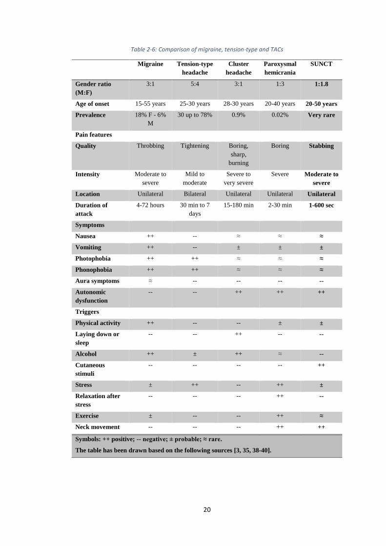
2.4. Presentation and comparison
Primary headaches represent more than 90% of headache complaints presented to
GPs. Although primary headaches are the most common, they are not serious or life
threatening. There are no distinguishable causes for primary headaches, and the
diagnosis is most often made by the history of headache as well as the associated
signs and symptoms. Primary headaches may share certain features; pain is severe
for migraine and CH as an example. However, CH varies from migraine primarily in
its pattern of occurrence. CH is in briefer episodes over a period of weeks or months.
Sometimes, a whole year can pass between two CHs. Migraine usually does not
follow this type of pattern. Consequently, and after a comprehensive study of the
literature of primary headaches, we decided to conclude this chapter with a thorough
comparison of the major types of primary headache disorders. Although there are
some intertwined features between them, such a comparison provides significant
support in distinguishing a particular type of headache from another.
Page 32
20
Table 2-6: Comparison of migraine, tension-type and TACs
Migraine Tension-type
headache
Cluster
headache
Paroxysmal
hemicrania
SUNCT
Gender ratio
(M:F)
3:1 5:4 3:1 1:3 1:1.8
Age of onset 15-55 years 25-30 years 28-30 years 20-40 years 20-50 years
Prevalence 18% F - 6%
M
30 up to 78% 0.9% 0.02% Very rare
Pain features
Quality Throbbing Tightening Boring,
sharp,
burning
Boring Stabbing
Intensity Moderate to
severe
Mild to
moderate
Severe to
very severe
Severe Moderate to
severe
Location Unilateral Bilateral Unilateral Unilateral Unilateral
Duration of
attack
4-72 hours 30 min to 7
days
15-180 min 2-30 min 1-600 sec
Symptoms
Nausea ++ -- ≈ ≈ ≈
Vomiting ++ -- ± ± ±
Photophobia ++ ++ ≈ ≈ ≈
Phonophobia ++ ++ ≈ ≈ ≈
Aura symptoms ≈ -- -- -- --
Autonomic
dysfunction
-- -- ++ ++ ++
Triggers
Physical activity ++ -- -- ± ±
Laying down or
sleep
-- -- ++ -- --
Alcohol ++ ± ++ ≈ --
Cutaneous
stimuli
-- -- -- -- ++
Stress ± ++ -- ++ ±
Relaxation after
stress
-- -- -- ++ --
Exercise ± -- -- ++ ≈
Neck movement -- -- -- ++ ++
Symbols: ++ positive; -- negative; ± probable; ≈ rare.
The table has been drawn based on the following sources [3, 35, 38-40].
Page 33
21
2.5. Secondary headache disorders
There is a definite underlying cause of secondary headaches that identifiable on
examination or investigation. Secondary headaches are very rare in comparison to
primary headaches; however, they are convoluted because they can lead to serious
complications. Secondary headache is a symptom of another disease that can activate
the pain-sensitive nerves of the head. Secondary headache has numerous causes
including head and neck trauma or injury; intracranial vascular disorders such as
ischaemic stroke, or non-vascular disorders such as high cerebrospinal fluid (CSF)
pressure (i.e. hydrocephalus), infection and psychiatric disorder, and disorder of the
cranium, neck, eyes, ears, nose, sinuses, teeth, mouth or other facial or cervical
structure [2-4, 22].
Headache attributed to idiopathic intracranial hypertension (IIH) or hydrocephalus is
an example of secondary headache. It was initially described in 1897 as a syndrome
of papilledema and elevated intracranial pressure attributed to impaired cerebrospinal
fluid (CSF) flow. Hydrocephalus is a neurological condition in which the
cerebrospinal fluid (CSF) is excessively accumulated around the brain, which can
lead to an enlargement of the ventricular system of the brain and increase the
pressure inside the head. It is caused by various etiological factors, however the
common final result is insufficient passage of cerebrospinal fluid (CSF) from its
point of production in the cerebral ventricles to its point of absorption into the
systemic circulation [41].
This excessive build-up of CSF yields a harmful pressure on the tissues of the brain.
In an adult human, there is approximately 150 cubic cm of CSF surrounds the brain,
the spinal cord and present in the ventricular system within the brain. The CSF
possesses many functional benefits such as protecting from mechanical stresses by
minimising the pressure inside the cranial vault induced brain expansion during
cardiac constriction. It is also supporting the brain weight by the buoyancy. CSF
protects the brain and spinal cord from shocks by acting as a cushion. Moreover CSF
plays an important role in the absorption and carrying away of the toxic by-products
of metabolism [42].
Page 34
22
2.6. Chapter summary
In this chapter, we have reviewed and understood the main types of primary
headaches including migraine, tension-type headache and TACs. Each of them
presented with its clinical features and diagnostic criteria based on the latest clinical
guidelines and references. This deep investigation of headache causes and patterns
leads to a comprehensive comparison that can highlight common and different
qualities of primary headaches. In general, it can be noted that the criteria of IHS is
the most agreed clinical guideline worldwide that is in use for clinical diagnosis of
headache disorders. These criteria also extensively used to establish almost all of the
diagnostic support modules.
Page 35
23
CHAPTER 3: LITERATURE REVIEW
3.1. Introduction
Over the last decades, information technology in general and artificial intelligence in
particular have gradually involved in every single field of life, starting from industry,
business, weather forecasting and media, but the most significant development has
taken place in the field of healthcare. Healthcare organisations are continually
endeavouring to improve patient care and provide better services. Introducing
information technology into healthcare delivery is expected to become an enabler to
get more efficient and effective healthcare services. Under the term of electronic
health (e-health), information and communication technology has changed the means
of patient care by providing home healthcare services with better infrastructure, cost
effectiveness and quality of services [43].
Currently, healthcare applications have expanded from (e-health) to mobile health
(m-health). The main driving force behind the change was the wide acceptance and
usage of smartphone mobile devices worldwide and a suitable platform and
environment for healthcare applications provided by these devices [44, 45]. This
chapter reviews the literature to investigate recent studies and decision support
systems (DSS) that target the diagnosis of primary headache disorders. This chapter
also compares and evaluates these relevant studies to explore their advantages and
drawbacks, which enable us to create a new diagnostic model that overcomes current
difficulties.
3.2. Intelligent driven modules to diagnose headaches
The development of clinical DSS to diagnose primary headache disorders has
become an interesting research topic, especially after the launch of the IHS clinical
criteria for the classification of headaches. A range of studies or diagnostic models
have been proposed or already developed to aid headache specialists in making
decisions with respect to the diagnosis of headaches. Many others were restricted for
patients’ usage such as an application to enable patients in keeping track of their
conditions and treatments or applications to get recommendations from health
Page 36
24
professionals. This section reviews the most recent studies that have been published
over the last decade.
3.2.1. Neurologist expert system (NES)
It is a rule-based DSS developed by Al-Hajji [46] to diagnose more than ten types of
neurological diseases including migraine and cluster headache. In this DSS,
knowledge has been obtained from different sources such as domain experts,
specialised databases, books and a few electronic websites. A list of neurological
diseases has been stored in a table and approximately 70 related symptoms were also
stored in another table. Then, a combination between each neurological disease and
its most related symptoms has been derived.
In fact, the diagnosis of many neurological diseases disease, such as Alzheimer’s,
Parkinson’s, Epilepsy, in addition to migraine and cluster headache, can be
challenging even for neurology specialists themselves. It is a wide range of diseases
that generally have shared symptoms and various diagnostic procedures. For
example, brain imaging can play a vital role in the diagnosis of Alzheimer’s or the
early detection of Parkinson’s disease. Moreover, there was no clear adoption of IHS
criteria with respect to the diagnosis of migraine and cluster headache. Therefore,
using a very simple link between each neurological disease and its symptoms cannot
be seen as an effective clinical DSS and would bear a large error rate.
3.2.2. Expert system based headache solution (ESHS)
An expert system was proposed by Hasan and his partners [47] to diagnose different
types of headache based on expert knowledge. ESHS includes a set of key questions
that derived from neurology experts to help other doctors when diagnosing patients
with headache. When symptoms are entered in accordance with these questions,
ESHS then would help in detecting the type of headache and generate prescriptions.
This expert system uses very simple yes/no questions derived from expert’s
knowledge instead of the globally agreed criteria of IHS. Moreover, the authors
failed to clarify who those experts are, and show their affiliations and experiences.
Page 37
25
3.2.3. A guideline-based DSS for headache diagnosis
A computerised headache guideline method was proposed by Yin and others [48] to
assist general practitioners in primary hospitals to improve the diagnostic accuracy of
primary headaches such as migraine, tension-type headache and cluster headache.
The main aim was to develop a system to counteract the complexity of the second
version of IHS criteria. Authors pass through three main steps to develop their
clinical DSS. A clinical specialist summarises the diagnostic guidelines of IHS and
expresses them as a flowchart in the first step. Then, a knowledge engineer
establishes a computerised model for headache knowledge representation based on
these flowcharts. Finally, the knowledge representation model is translated into a
series of conditional rules, which are used by the inference engine. This clinical DSS
evaluated by 282 previously diagnosed headache cases obtained from a Chinese
hospital.
3.2.4. Validation of a guideline-based DSS for headache diagnosis
In 2014, Dong and his colleagues have developed a guideline-based clinical DSS for
headache diagnosis [49]. They have followed the same procedure presented in [48]
for knowledge acquisition, but using the third version of IHS criteria and validated
their system by 543 data sheet of patients with headache obtained from the
International Headache Centre at the Chinese PLA General hospital, Beijing, China.
The main difference between this guideline-based DSS and the guideline-based DSS
developed by Yin in [48] is that three more types of headache have been added to the
library of this DSS including probable migraine, probable tension-type headache,
new daily persistent headache and medication overuse headache. As shown in [49],
there was some improvement in the diagnosis in comparison with DSS by Yin in
[48].
3.2.5. Case-based reasoning DSS for headache diagnosis
A computer-aided diagnosis method was proposed by Yin et al. [50] and employs
case-based reasoning (CBR) method to differentiate between probable migraine and
probable tension-type headache. This CBR clinical DSS provides recommendations
to the general practitioners based on the previously solved cases in the built-in
library. This library contains 676 data sheets of patients with probable migraine and
Page 38
26
probable tension-type headache that were collected by clinical interview. Each data
sheet consists of 74 different attributes including patients’ information and medical
history in addition to headache symptoms derived from the IHS criteria. The authors
employ genetic algorithm (GA) to assign weights to these attributes and K-nearest
neighbour (KNN) method to measure the similarity between new headache cases and
the previous cases in the library.
3.2.6. Hybrid intelligent reasoning DSS
A hybrid DSS tool was proposed by Yin and his partners [51] using a combination of
rule-based and case-based reasoning methods to improve the diagnosis of primary
headache disorders such as migraine, tension-type headache and cluster headache.
The reasoning modules in this clinical DSS run independently, the rule-based module
is the first diagnostic module and the case-based module is the second. The
diagnostic rules are summarised by a clinical specialist based on the criteria of IHS
in the first module, while data sheets of previous headache cases have been used in
the second module. The diagnostic procedure starts through applying the first
diagnostic module to a new headache case, if headache symptoms are typical and
match the existing rules, then a diagnostic decision can be made. Otherwise, the
headache case is transferred to the case-based module to search for the most similar
previous cases.
The research group in [50] claim that the CBR clinical DSS shows an improvement
with respect to the diagnosis of primary headaches when compared to their previous
works [48, 49] that were built around the guideline-based concept. Although the core
concept of [48, 49] and [50] seems to be similar, however knowledge acquisition
methods are completely different. In [48, 49], the specialist derives diagnostic
guidelines from IHS criteria, which is then expressed as a set of conditional rules,
while [50] uses clinical interviews of patients with headache as a knowledge
acquisition stage. The same research group have also proposed a hybrid clinical DSS
in [51], which is a merger of their previous proposals in [48, 49] and [50].
3.2.7. Automatic DSS for the classification of primary headaches
This is a machine learning based DSS proposed by Krawczyk and his colleagues [52]
to support the classification of primary headaches. The main aim of this study was to
Page 39
27
distinguish between the episodic tension-type headache and migraine without aura.
Authors have prepared a questionnaire according to the second version of the criteria
of IHS as a knowledge acquisition stage. The questionnaire includes general
information of patients such as age, gender, marital status, level of education, etc., in
addition to questions that related to headache characteristics such as frequency of
attacks, quality of pain, associated symptoms, headache location, intensity and
triggers. Six machine-learning algorithms were applied to the collected data
including Naïve Bayes, Decision Tree (C4.5), Support Vector Machine, Bagging,
Boosting and Random Forest. Using the 10-fold cross validation method, the
experiment showed that the best result could be achieved through a combination of
Random Forest method with Bagging and/or Boosting methods.
3.2.8. Other headache diagnostic modules
Simić and others in [53] and [54] have proposed a computer-assisted diagnosis of
primary headaches. It is a rule-based fuzzy logic (RBFL) system designed to help
physicians when diagnosing patients with primary headaches such as migraine,
tension-type headache and cluster headache. This work involves under the type of
knowledge-based DSS, in which the criteria of IHS are expressed as a collection of
IF-THEN statements. Another group of researchers in [55] trained artificial neural
networks to diagnose migraine, tension-type headache and medication overuse
headache. The artificial neural networks have been trained using questionnaire-based
data collected from patients with headache.
Ufuk and others in [56] have evaluated an immune algorithm for the classification of
migraine, tension-type headache and cluster headache. A website based survey
expert system was used to collect data of patients with primary headaches. They
conclude that the immune algorithm can help the neurologist with respect to the
classification of primary headaches.
Eslami and his partners in [57] have designed a computerised expert system to help
in the diagnosis of primary headache disorders such as migraine, tension-type
headache, cluster headache and other trigeminal autonomic cephalalgias. A
questionnaire was designed to approach all criteria of primary headache disorders
based on the second version of IHS criteria. When a patient starts filling in the
questionnaire, the expert system uses a simple human-like algorithmic reasoning to
Page 40
28
classify the type of headache. Similarly, Maizels and Wolfe in [58] employ a simple
human-like branching logic to determine the most appropriate diagnostic questions to
ask the patients, then, classify the type of headache using modified Silberstein Lipton
criteria and IHS criteria. Maizels and Wolfe implemented their expert system as a
web-based tool with an interview section that includes questions about headache
characteristics. The modified Silberstein Lipton criteria are used to classify patient
with frequent headache, while IHS criteria are used to diagnose patients with brief
headache syndromes.
Zafar and others in [59] proposed a clinical DSS to aid physicians in the diagnosis of
migraine and other headaches and at the same time to enable patients living in
remote areas to have medical check-ups. Zafar implemented his work as a web-based
tool, in which information related to primary and secondary headaches are stored in
the knowledge base. The inference engine will search this knowledge base to find
suitable diagnostic recommendations based on headache characteristics. This
proposed system, in fact, is considered as a black box because there is no clear
sequence of operations in particular for knowledge acquisition.
3.3. Evaluation and justifications
Decisions taken made by headache specialists usually depend on clinical guidance,
medical evidence, instructions and principles derived from medical science. In an
ideal situation, clinical DSS should improve the use of knowledge to support those
specialists in making more accurate decisions, and therefore enhancing the quality of
care being delivered to the patient. Although clinical DSS have a potential to
improve decision making, handling large amount of information and analysing real-
time data or patient history, however, the use of clinical DSS is not yet widespread in
clinics or hospitals. This might be because the majority of such systems are
developed apart from healthcare professionals and there is lack of criteria for a
proper use of intelligent methods in these clinical DSS [60].
Page 41
29
Figure 3-1: Types of clinical decision support systems
In general, we can categorise clinical decision support systems into three main
groups as shown in figure 2-1. Knowledge-based clinical DSS is the first, machine
learning based clinical DSS is the second, and hybrid clinical DSS that is based on a
combination of the first two groups. The Knowledge-based DSS is designed and
structured around the logic of IF-THEN statements, in which clinical guidelines such
as IHS criteria or experts' knowledge are formed into rules and expressed by a
computer engineer as a set of IF-THEN-ELSE statements. This usually includes a
significant amount of information regarding the types of headache together with their
signs and symptoms. Once the patient data are input, the inference engine examines
the data against these IF-THEN statements to limit the outcome response.
A simple example of using knowledge based DSS presented in [61], in which the
DSS includes a probable list of haematological diseases combined with their
symptoms. Inputs to this CBC clinical DSS include patient information such as age,
gender, altitude, pregnancy period in addition to the complete blood count (CBC) test
result. The inference engine will suggest a list of probable haematological diseases
based on these inputs. Although it is unable to provide an ultimate diagnosis,
however, it is a good start for further and more disease-specific tests to confirm the
diagnosis.
Going back to the diagnostic modules that are summarised in table 2-1, the core
concept of the majority of them was approximately similar regarding the knowledge
acquisition, where the international classification of headache disorders was used as
Page 42
30
a base for deriving the diagnostic rules. These rules were summarised and expressed
by a computer engineer. This style is commonly known as a rule-based method, by
which the rules are formulated based on a human expert. The basic principle of the
rule-based technique is pattern identification followed by a recommendation of what
should be done in response. These rules are a conditional statement that links the
supplied conditions to actions or results. Ideally, the rule is straightforward,
understandable and represents the knowledge in near-linguistic form [60].
Table 3-1: Summary of diagnostic modules
No. Authors Year Type of
module
Knowledge Type of headache
1 Al-Hajji [46] 2012 Knowledge-
based
Domain experts MIGR and cluster
headache
2 Hasan et al. [47] 2012 Knowledge-
based
Domain experts Primary headaches
3 Yin et al. [48] 2013 Knowledge-
based
IHS criteria Primary headaches
4 Dong et al. [49] 2014 Knowledge-
based
IHS criteria Primary headaches
5 Yin et al. [50] 2015 Knowledge-
based
Case-based
similarity
Probable MIGR
and probable TTH
6 Yin et al. [51] 2014 Knowledge-
based
Case-based and
IHS criteria
Primary headaches
7 Krawczyk et al. [52] 2013 Machine
learning
IHS criteria Episodic TTH and
MIGR without aura
8 Simić et al. [53, 54] 2008 Knowledge-
based
IHS criteria Primary headaches
9 Mendes et al. [55] 2010 Machine
learning
Questionnaire Primary headaches
10 Ufuk et al. [56] 2016 Knowledge-
based
Survey data Primary headaches
11 Eslami et al. [57] 2013 Knowledge-
based
Questionnaire Primary headaches
12 Maizels and Wolfe
[58]
2008 Knowledge-
based
Silberstein Lipton
criteria and IHS
criteria
Primary headaches
13 Zafar et al. [59] 2013 Knowledge-
based
Unknown Primary and
secondary
headaches
Page 43
31
The rules-based system style can facilitate the separation of knowledge from
processing, in addition to allowing incomplete or uncertain knowledge to be
expressed and bounded. However, implementing this kind of system could possibly
carry certain downsides. First, rule-based systems are not able to learn and modify
their rules from experience or via identifying patterns in clinical data. Secondly,
navigating the categorisations and relationships in a large rule-based system can be
complicated and time consuming. Third and the most important point is that the
necessary information needed to derive these diagnostic rules might consist of more
variables than the human mind can accommodate. There is persuasive evidence to
indicate that the human ability to discover and understand complicated configuration
relationships could be limited [62].
Therefore, deriving and formulating these diagnostic rules, with the limited ability of
human mind to manipulate a large quantity of information or variables in considering
a complex subject such as IHS criteria, may lead to insufficient representation of
knowledge and eventually a poor diagnostic model [60]. Moreover, we would like to
pay attention to the fact that the IHS criteria are designed to provide a ground truth
for headache specialists, where this classification of headaches provides clear distinct
definitions describing many different types of headache. However, these types of
headache may share signs and symptoms in real world scenario and they also my
change over time, which makes the classification of primary headaches not as clear
as black or white (i.e. as we show in the procedural classification function). This
means that there is a grey area in between, which can affect the diagnostic
performance, validity and reliability of decisions made by such CDSMs. In this
context; we are adopting a completely different approach, in which several machine-
learning classifiers were applied to diagnose primary headache disorders using
anonymised real-world data records of patients with primary headaches.
3.4. Chapter summary
In this chapter, we reviewed the literature to explore studies and decision support
systems (DSS) that target the diagnosis or classification of primary headache
disorders. The majority of these studies or systems have followed a rule-based
system style, in which a computer engineer formulates the diagnostic rules as a set of
IF-THEN-ELSE statements based on clinical guideline or prepared questionnaire.
Page 44
32
Although the rule-based system style is straightforward, understandable and can
represent the knowledge in near-linguistic form, however, it bears many serious
downsides such as the inability to learn and gain knowledge over time and
maintaining categorisations and relationships in a large rule-based system can be
complicated. Therefore, we will avoid such a style of diagnostic models via the
implementation of machine learning methods.
Page 45
33
CHAPTER 4: DATA PREPARATION
4.1. Introduction
Since the data is a building block of every information system, a first step in the
application of machine learning is to examine the characteristics of the data, which is
commonly known as a data processing stage. In general, there are two main types of
data in scientific researches, quantitative and qualitative. Quantitative data are the
data that express items of interest numerically and quantitative research involves
examining causal relations, patterns and associations in such data using statistical
methods [63]. In quantitative data, measurement units are often used to represent
observations, for example patients’ age measured in years, patients’ height measured
in meter or inches, duration of pain measured in minutes or hours, years of suffering
and so on.
In contrast, qualitative data is typically descriptive and it represents numbers of
cases, scenarios, events, experiences using data from observations or interviews. In
quantitative research, the phenomena examined cannot be fully comprehended
through quantification. For instance, how do patients describe their headache
characteristics? Where is the location of pain? Did patients or any of first-degree
relatives suffer from a particular chronic condition? Qualitative research involves
examining answers to these types of questions for a particular condition in order to
understand patients’ experience [63].
This chapter describes the process of knowledge acquisition. It begins by describing
the data set, and then emphasises all potential key concerns that ought to be
addressed in the pre-classification stage. In this chapter, we identify and process
outliers in data, then, handle missing data using multiple imputations, and we end
this chapter by normalising the data using min-max normalisation method.
4.2. Data description
This study re-uses the data set in [64] for the following reasons; a) the dataset has
been collected by headache specialists in three medical-academic centres in Turkey
(i.e. School of Medicine - Mersin University, Medical Faculty - Istanbul University
and Istanbul Education Hospital). These centres combine clinical care with scientific
Page 46
34
research. b) It is high dimensional data with 65 dimensions, which covers a wide
range of patients’ information including medical history, family history and
psychological conditions, where such dimensions have not been covered in previous
studies. c) The data set involves patients with the most common primary headache
disorders including migraine with and without aura, chronic and episodic tension-
type headache, trigeminal autonomic cephalalgias TACs (i.e. cluster headache,
paroxysmal hemicranias and SUNCT). This diversity of patients has not been
addressed in previous studies as well. Finally, d) the data set was collected with the
aim of identifying a new sub-group of patients with vestibular symptoms in primary
headache disorders, where it is ideal for diagnostic purposes.
The data set consists of 832 records of patients with primary headache disorders, and
each record involves 65 attributes, including class attribute, as shown in table 4-1.
We can group patients’ records into three main categories. The first category
includes patients with tension-type headache. It is the largest group of patients and
includes 383 records, which represents 46.03% of the data. Out of 383 records, 221
records are for patients with episodic tension-type headache and 162 records are for
patients with chronic tension-type headache. The second category includes patients
with migraine, which consists of 378 records. It constitutes 45.43% of data. More
than two-thirds of the second group are for patients with migraine without aura, i.e.
around 300 records. The remaining 78 records are for patients suffering from
migraine with aura.
The last category of records is for patients with TACs, which comprises of 71
records and represents 8.54% of the data. These 71 records are distributed as follows;
53 records are for patients with cluster headache, 12 records are for patients with
paroxysmal Hemicrania and six records for patients with SUNCT. The number of
records for patients with TACs is considerably less than other records (i.e. patients
with migraine and tension-type headache). It is naturally inherited because the
occurrence of TACs is very rare in comparison with other primary headache
disorders. However, this can lead to an imbalanced class distribution that may affect
the learning approach. We will discuss and handle this issue further in the next
chapter.
Page 47
35
Table 4-1: Data attributes
No. Data attributes Level of
measurements
Descriptions
1 Gender Dichotomous Male/Female
2 Age Numerical Calculated in years
3 Age of admission Numerical Calculated in years
4 Diagnosis Categorical Type of primary headache – Class attribute
5 Headache onset Numerical Calculated in months
6 Headache frequency Numerical Days per month
7 Headache characteristic Categorical Throbbing, Pressing, Dull, Stabbing, lightening
8 Headache duration Numerical Calculated in hours
9 Headache location Categorical Unilateral, Bilateral, Frontal, Periocular, Bi-
temporal, Occipital, Calvarial
10 Headache intensity Numerical Visual analogue scales (VAS) 1-10
11 Accident Dichotomous Present/Absent
12 Periodic vomiting Dichotomous Present/Absent
13 Motion Sickness Dichotomous Present/Absent
14 Abdominal pain Dichotomous Present/Absent
15 Epilepsy Dichotomous Present/Absent
16 Surgery Dichotomous Present/Absent
17 Allergy Dichotomous Present/Absent
18 Homocysteinemia1 Dichotomous Present/Absent
19 TIA/Stroke2 Dichotomous Present/Absent
20 Atherosclerosis3 Dichotomous Present/Absent
21 Hyperlipidaemias4 Dichotomous Present/Absent
22 Oral contraceptive Dichotomous Present/Absent
23 Hypertension Dichotomous Present/Absent
24 Diabetes Dichotomous Present/Absent
25 Coronary Artery disease Dichotomous Present/Absent
26 Snoring Dichotomous Present/Absent
27 OSAS5 Dichotomous Present/Absent
28 Infantile colic6 Dichotomous Present/Absent
29 Medication overuse Dichotomous Present/Absent
30 Pain killer using frequency Numerical The frequent usage of painkiller per month.
31 Medication overuse duration Numerical Calculated in months
32 Headache Dichotomous Present/Absent 33 Hypertension Dichotomous Present/Absent 34 Atopic disorder7 Dichotomous Present/Absent 35 Diabetes Dichotomous Present/Absent 36 Heart disease Dichotomous Present/Absent 37 Epilepsy Dichotomous Present/Absent 38 Psychopathology8 Dichotomous Present/Absent 39 Smoking Dichotomous Yes/No
40 Smoking duration Numerical Calculated in years
41 Emotional stress Dichotomous Present/Absent 42 Physical activity Dichotomous Present/Absent 43 Menstrual cycle Dichotomous Present/Absent 44 Seasonal Dichotomous Present/Absent 45 Alcohol Dichotomous Present/Absent 46 Skipping meals Dichotomous Present/Absent 47 Positional association Dichotomous Present/Absent 48 Nausea Dichotomous Present/Absent 49 Vomiting Dichotomous Present/Absent 50 Phonophobia Dichotomous Present/Absent 51 Photophobia Dichotomous Present/Absent 52 Dizziness Dichotomous Present/Absent 53 Sleep disturbances Dichotomous Present/Absent
Page 48
36
54 Vertigo Dichotomous Present/Absent 55 Osmophobia9 Dichotomous Present/Absent 56 Allodynia10 Dichotomous Present/Absent 57 Normal Dichotomous Present/Absent 58 Anxiety Dichotomous Present/Absent 59 Depression Dichotomous Present/Absent 60 Obsession Dichotomous Present/Absent 61 Psychosis Dichotomous Present/Absent 62 Fundoscopy Dichotomous Normal/Abnormal
63 Fundoscopy explanation Numerical Comments
64 Neurological examination Dichotomous Normal/Abnormal
65 Pericranial muscle tenderness Dichotomous Present/Absent
1 Abnormally high levels of Homocysteine in the serum, above 15 µmol/L. 2A transient ischemic attack (TIA), also called a mini stroke, occurs when a blood clot blocks blood
flow in the brain. 3A serious condition where arteries become narrow or clogged up by fatty substances known as plaques
or atheroma. 4Elevated lipid levels in the blood. 5Obstructive Sleep Apnoea syndrome, a condition where the walls of the throat relax and narrow during
sleep, interrupting normal breathing. 6Distress or crying in an infant, which lasts for more than three hours a day, for more than three days a
week, for at least three weeks in an otherwise healthy infant. 7The genetic tendency toward developing a classical allergic diseases including; atopic dermatitis,
allergic rhinitis, and asthma. 8A study of mental disorders. 9Refers to a fear, aversion or psychological hypersensitivity to odours. 10An abnormal sensation, in which patients feel pain from something that shouldn't be painful. 11Also called Ophthalmoscopy, is a test that allows a doctor to see inside the back of the patient’s eye
and other structures using a magnifying instrument and a light source.
Headache data set includes a combination of quantitative and qualitative data
described using different levels of measurement, such as numerical, dichotomous and
categorical. Although the levels of measurement differ in many ways, they are
unifying both quantitative and qualitative data into four different levels of
measurement or scales [65]. Categorical and dichotomous scales are within the scope
of qualitative attributes, numerical scales are belonging to quantitative attributes
[66]. These categories convey a different amount of information. In fact,
measurement is the method of assigning numbers or labels to items of interest in
order to make the data amenable to statistical analysis and machine learning
requirements [65]. However, the majority of machine learning algorithms are merely
supporting numerical attributes, which require converting nominal attributes into a
format that could be supported by these learning algorithms. In other words,
providing the data in a numerical representation. Therefore, the categorical and
dichotomous variables were dummy coded. For example, the absence of a certain
condition was coded as zero; in contrast, the presence of that condition was coded as
one.
Page 49
37
4.3. Outliers’ detection
Outliers are strange data points that are distant from other members of a given data
cluster [67]. In general, outliers may arise from procedural error, such as inaccurate
data collection, or they can be inherited from the natural variance of the data.
Osborne and Amy [68] have described a number of other causes that may lead to
outliers, while Zhao [69] identifies many different methods to detect outliers
including visual inspection via plots, clustering and local outlier factor.
This study follows the visual inspection manner and uses box and whisker plot
(usually known as boxplot) to detect outliers. Boxplot is a straightforward way that
graphically depicts clusters of data points via their quartiles. Boxplot employs
median and interquartile range IQR to detect the outliers, where the median is the
middle number of an ordered set of numbers and the interquartile range is the
variance between the first and third quartiles. In the boxplot, outliers are the data
points that are located beyond the extremes of the whiskers [69]. To be more precise,
outliers are the data points that fall above Q3 + 1.5(IQR) and below Q1 − 1.5(IQR),
where Q1 is the first quartile, Q3 is the third quartile, and IQR = Q3 − Q1.
This section plots the data variables in accordance with the types of headache to
assist in determining the outliers for each group of patients separately. This is mainly
because different types of headache have different ages of onset, features, durations
and intensity. Therefore, plotting variables with three major types of headache as a
bunch would lead to inaccurate identification of outliers. Figure 4-1 shows the
outliers within continuous variables, i.e. quantitative attributes, where circles
represent outliers while stars refer to extreme outliers. The Box plot displays outliers
and extreme outliers with their record numbers.
Outliers are usually handled in one of three methods. First, retain the outliers and
handle them just like every other data point. Second, trimming them (i.e. remove
outliers from the sample) and third, winsorising them [70]. Retaining outliers and
handling them just like every other data point may overvalue them and lead to
estimates that significantly vary from the legitimate population value. Trimming
outliers is a very common practice in the literature; however, it may not be an
appropriate way when the outliers are legitimate values [71]. The trimming method
assumes that outliers are due to mistakes. For example, the measurement of a given
Page 50
38
variable could be entered as 10000 instead of 100.00, which can cause a huge change
in the estimates. Therefore, this method is usually recommended for outliers due to
typographical mistakes or measurement errors. Furthermore, trimming outliers is
generally unacceptable because they can be legitimate observations and may signify
the natural variance of data. On the other hand, winsorising is a common procedure
to handle outliers via modifying them to the next highest or lowest values within the
distribution that are not suspected to be outlier [72]. Winsorising is recommended
when the outliers are valid data points, i.e. legitimate observations [70].
There are controversies regarding the decision to keep or remove outliers, where
there is no definitive answer to the problem. Some researchers recommend
eliminating all outliers to ensure that the parameter estimates are more related to the
target population, while others encourage retaining, in particular, legitimate outliers
[68, 70]. Osborne and his partner [68] have described how a small percentage of
outliers can significantly affect even simple analyses, where they have reported that
outlier removal enhances the accuracy of estimates for correlations and t-tests, while
it greatly reduces errors of inference.
On the other hand, Dhiren and his colleague [70] reported that winsorising by 2.5%
would maintain the characteristics of the data and not really change the distribution
very substantially. Moreover, they have mentioned that winsorising would alleviate
bias by preserving an attenuated version of the outlier rather than eliminating it. In
general, outliers may pose critical problems to data analysis. For example, a normal
distribution assumption is required for parametric analysis methods and the presence
of outliers usually contributes to violate such assumptions, particularly for regression
analysis, where outliers can significantly affect the slope, R-value and R Square
estimates. Furthermore, outliers can increase the variance of data and therefore
minimise the power of statistical tests, which is undesirable.
Page 51
39
Figure 4-1: Data outliers
Before handling outliers, we need to understand why they exist. As shown in figure
4-1, there are a miniscule number of outliers in the headache data set (0.48% of age,
0.60% of headache frequency, 0.72% of headache intensity and admission age,
2.40% of headache onset and 3.24% of headache duration). Comparing these outliers
to the criteria of the International Headache Society (i.e. ICHD-3 beta)[3] revealed
that some of them are legitimate extreme observations, which may be inherited from
the arbitrary sampling of patients.
Page 52
40
For example, the age of onset for migraine patients can range from 15 up to 55 years
according to ICHD-3 beta, while the highest observed outlier for migraine patients
within the data set was 50 years (record number 805). In contrast, some other outliers
exceed the range that was identified by ICHD-3 beta. For instance, the age of onset
for patients with tension-type headache may range from 25 to 30 years according to
ICHD-3 beta, compared to 50 years age of onset (record number 800), which was the
extreme observed outlier for patients with tension-type headache in the data set.
Furthermore, let us consider headache duration as another example, where the
extreme observed outlier was 360 hours of headache duration for patients with
migraine (record number 579), compared to 72 hours as a maximum duration of
migraine based on ICHD-3 beta. On the other hand, many other outliers such as
record 481 and record 733 fell within the range of duration that was identified by
ICHD-3 beta.
Although some outliers represent valid observations, nevertheless, extreme outliers
would drastically influence the normality of the data and possibly one extreme
outlier can skew the data by a large amount. Therefore, we measured the skewness of
the data variables with and without outliers to examine whether outliers could skew
our data. In general, the exclusion of extreme outliers seems to decrease variance and
degree of skewness remarkably, while maintaining the mean. The skewness of some
variables dropped by more than 50%. For example, the skewness of age variable was
0.628, compared to 0.305 without three extreme outliers only. The skewness of
headache duration variable decreased from 4.048 to 1.801 when excluding six
extreme outliers only. Likewise, the variance of age and headache duration variables
reduced by 16.88, 173.47 respectively. Furthermore, the skewness of age of
admission variable dropped by 75% from 0.641 to 0.170, and the variance decreased
by 41.63 because of excluding three extreme outliers only.
On the other hand, the mean age, age of admission and headache duration variables
were very similar. The mean age was 44.98, compared to 44.73 without extreme
outliers. Similarly, 37.40 was the mean age of admission, compared to 37.14 when
excluding extreme outliers. Finally, the mean headache duration dropped by 0.82%.
Thus, it was clear that only a few extreme outliers could significantly influence the
distribution of the data as well as raise the degree of skewness dramatically.
Page 53
41
Figure 4-2: Data without outliers
Consequently, we have decided to winsorise the outliers instead of excluding them,
as we believe that the presence of outliers in the headache data set is due to the
nature of data. Therefore, winsorising outliers, as shown in figure 4-2, would make
them closer to the data points through modifying them to the next highest or lowest
values that are not presumed to be outlier. As described in [70], winsorising a small
number of outliers, i.e. just like our case, would not violate the characteristics of
data. However, it would maintain the sample size in particular when the outliers are
Page 54
42
legitimate observations. In data pre-processing steps, detecting outliers and
addressing them was the first step because they can significantly influence other
stages of data processing. For example, the existence of outliers can affect the
imputation process, where many other outliers can be produced by imputation.
4.4. Missing Data
Missing data or missing values are very common in real-world data sets, particularly
in medical datasets [73]. According to Tran and his colleagues [74], 45% of the data
sets in the online data repository UCI have some sorts of missing values. Missing
data can occur due to many reasons such as unexpected difficulty in getting some
vital measurements. Participants may refuse to answer some questions. The research
team may be unable to follow-up all participants during the period of study.
Participants' records lack some values due to failure of electronic data storage, and
collecting data from heterogeneous sources such as different medical centres, which
is the case for our data set. All of these reasons along with many other hidden causes
can lead to data losses [75, 76].
Missing data can give rise to serious concerns for classification, where the main
concern is the non-applicability of many classification algorithms for such data.
Although some algorithms can handle data with missing values by ignoring them,
however the majority cannot. Consequently, waste of data and significant
classification errors are most likely to occur [77]. Therefore, the first step toward a
valid classification process is addressing the issue of “missing data”, but we need to
consider the nature of the missing data mechanism first, which is a fundamental step
to get a valid inference from incomplete data.
4.4.1. Missing data mechanism
A missing data mechanism identifies how the underlying value of missing
observation is connected with the reason for being missing [78]. Let us assume 𝑌 is
𝑁𝑥𝑃 matrix containing the data values of 𝑃 variables (i.e. attributes) for all 𝑁 units
or participants in the sample. Each units denoted by 𝑌𝑖 = (𝑌𝑖1, 𝑌𝑖2, … , 𝑌𝑖𝑃). No matter
whether the type of response falls under quantitative or qualitative data, 𝑌𝑗 represents
the 𝑗𝑡ℎ measurement for the 𝑖𝑡ℎ subject or participant at time 𝑇𝑖𝑗, where 𝑖 = 1, … , 𝑁
and 𝑗 = 1, … , 𝑃, and 𝑌−𝑗 represents all columns in 𝑌𝑖 except 𝑌𝑗 (i.e. the complement
Page 55
43
of 𝑌𝑗). The missing values in 𝑌𝑖 are collectively denoted as 𝑌𝑖𝑚, while the observed
values in 𝑌𝑖 are collectively denoted by 𝑌𝑖𝑜, therefore 𝑌 = ( 𝑌𝑚, 𝑌𝑜) hypothetically
represents complete data values. Nevertheless, the values of the part 𝑌𝑚 are
unknown for different reasons, and the data accordingly are incomplete [79]. In
1976, Rubin has identified three types of mechanisms under which missing data can
occur: First, missing completely at random (MCAR). Second, missing at random
(MAR). Third, not missing at random (NMAR) [80].
Data is considered to be missing completely at random (MCAR) when the likelihood
that responses are missing is unrelated neither to the observed values, nor to other
missing values. In other words, the missing response is independent of both 𝑌𝑖𝑜
and 𝑌𝑖𝑚, which means that the missing values of 𝑌𝑖 merely occurred by chance.
Unlike MCAR, data deemed to be missing at random (MAR) when the likelihood
that responses are missing depends only on a set of observed values rather than
certain missing values. That is, the missing response is merely the result of a chance
mechanism that does not depend on the values of another unobserved response. In
particular, missing data fall under MAR when the missing response is conditionally
independent of 𝑌𝑖𝑚, but not 𝑌𝑖
𝑜. If missing data is not classified as MCAR or MAR,
then we are talking about not missing at random (NMAR), which is the third type of
missing data mechanism. Missing data is perceived as NMAR when the likelihood
that responses are missing depends on both of the following; first, the values that
should have been obtained and second, the values that have been actually obtained.
To be more precise, missing response is related to 𝑌𝑖𝑚 and 𝑌𝑖
𝑜 [79, 81].
The significant feature of MCAR is that the observed data 𝑌𝑜 can be perceived as a
random sample of the complete data 𝑌. Thus, the observed data inherits the same
moments and joint distribution of the corresponding complete data. Consequently,
discarding or ignoring missing values 𝑌𝑚 under MCAR would not lead to bias,
however it most likely increases the standard error of estimations as a consequence
of reduced sample size [79, 81]. Therefore, the observed part of data 𝑌𝑜 can be used
to obtain valid estimates of moments, including; mean, variance, and covariance
[79].
In contrast to MCAR, the conditional distribution of Yio for subjects with any Yi
m
pattern in MAR would not coincide with the distribution of the corresponding
Page 56
44
components of 𝑌𝑖 in the target population. Consequently, the observed data Yo cannot
be thought of as a random sample of the complete data Y. Therefore, calculating
mean, variance, and covariance only based on the observed part of data Yo can lead
to biased estimates [79, 82]. MAR and MCAR are showing, in general, the missing
response patterns at random and they are usually referred to as ignorable
mechanisms, in which the missing values Ym can be avoided or deleted [73, 81].
Conversely, NMAR mechanism is usually known as a non-ignorable mechanism, in
which the missing value Ym cannot be avoided or deleted because the goal is to make
inferences about the distribution of the complete data Y. Therefore, MCAR
mechanism seems to pose less threat to statistical inferences in comparison with
MAR and MNAR [79, 81].
Figure 4-3: Overall summary of missing data
The headache data set as shown in figure 4-3 has 98% of its variables (i.e. attributes)
coming with missing values and 100% of cases have some sorts of missingness.
Different rates of missingness has been shown, starting from less than one percent
for some variables and reaching 100% for some others. Table 4-2 illustrates the
missingness rate in descending order. At the bottom of the table, gender and age
variables came with missing rates of 1% and 2% of respectively, this seems unrelated
to other aspects such as socioeconomic status, disciplinary problems, or any other
study-related attributes. However, it is most likely caused by an administrative
mistake or a data storage failure.
Page 57
45
On the other hand, we have noticed considerably high missing rates in attributes that
are related to historical queries, for example asking patients whether they suffered
from infantile colic, such responses may not be known for patients themselves,
particularly for older patients. This is quite a common type of missing values, where
responses are usually "Don't know" or questions are skipped. At the top of the table,
some variables are completely missing for example, Fundoscopy explanation
variable is 100% missing despite that Fundoscopy variable showed only 13%
missing rate. This could be due to the difficulty of interpreting and converting a
countless Fundoscopy explanation into numerical or categorical representations.
Psychosis is another variable with 100% of missingness. The research team was
aiming to collect this variable at the start of their study; however, it might have been
left blank because it requires detailed explanation of test results or perhaps due to
time limits.
Table 4-2: Variable Summary a,b
Missing Valid
N
Mean Std.
Deviation N Percent
Fundoscopy explanation 832 100.0% 0
PC Psychosis 832 100.0% 0
Medication overuse duration 818 98.3% 14 3006.64 11128.535
Pain killer using frequency 813 97.7% 19 40.89 60.688
PC Obsession 793 95.3% 39
MH Infantile colic 758 91.1% 74
PC anxiety 745 89.5% 87
Smoking duration 719 86.4% 113 8.075 8.2773
MH OSAS 661 79.4% 171
MH Snoring 659 79.2% 173
Medication overuse 642 77.2% 190
PC normal 625 75.1% 207
Pericranial muscle tenderness 572 68.8% 260
PC Depression 554 66.6% 278
FH Psychopathology 537 64.5% 295
FH Atopic disorder 537 64.5% 295
FH Epilepsy 528 63.5% 304
FH Heart disease 504 60.6% 328
FH Diabetes 492 59.1% 340
MH Oral contraceptive 489 58.8% 343
S Allodynia 486 58.4% 346
S Osmophobia 479 57.6% 353
MH Coronary Artery disease 471 56.6% 361
MH Diabetes 462 55.5% 370
T Alcohol 461 55.4% 371
FH Hypertension 455 54.7% 377
MH Hypertension 428 51.4% 404
T Skipping meals 425 51.1% 407
Page 58
46
FH Headache 350 42.1% 482
MH Homocysteinemia 174 20.9% 658
MH Allergy 161 19.4% 671
MH TIA/Stroke 151 18.1% 681
MH Periodic vomiting 147 17.7% 685
MH Atherosclerosis 144 17.3% 688
MH Epilepsy 144 17.3% 688
MH Motion Sickness 143 17.2% 689
MH Abdominal pain 142 17.1% 690
MH Surgery 139 16.7% 693
MH Accident 135 16.2% 697
MH Hyperlipidaemias 134 16.1% 698
S Sleep disturbances 115 13.8% 717
Fundoscopy 112 13.5% 720
S Vertigo 110 13.2% 722
T Positional association 106 12.7% 726
T Seasonal 97 11.7% 735
Smoking 91 10.9% 741
S Dizziness 85 10.2% 747
T Physical activity 84 10.1% 748
Headache intensity 73 8.8% 759 7.29 1.767
T Menstrual cycle 56 6.7% 776
Neurological examination 48 5.8% 784
T Emotional stress 43 5.2% 789
Headache duration 37 4.4% 795 18.3996 18.86362
Headache onset 34 4.1% 798 79.306 79.9491
Headache frequency 26 3.1% 806 10.161 9.0164
Headache characteristic 23 2.8% 809
Headache location 22 2.6% 810
S Vomiting 20 2.4% 812
S Photophobia 16 1.9% 816
S Phonophobia 16 1.9% 816
Age of admission 16 1.9% 816 37.24 12.903
Age 15 1.8% 817 44.83 13.825
S Nausea 8 1.0% 824
Gender 7 0.8% 825
a. Maximum number of variables shown: 65
b. Minimum percentage of missing values for variable to be included: 0.0%
Although the above assumptions mostly refer to random mechanisms of missing
response (i.e. MCAR or MAR), however further examination is required to identify
the specific mechanism that the data belongs to. Accordingly, we have employed the
separate-variance 𝑡 test to help in identifying the variables whose pattern of
missingness might be influenced by other quantitative variables [83]. The separate-
variance 𝑡 tests table showed that Osmophobia was most likely to increase the
duration of headache, when Osmophobia was missing; the mean headache duration
was 17.82, compared to 24.23 when Osmophobia was non-missing. Similarly, the
Page 59
47
duration of medication overuse was directly proportional to the duration of headache,
when medication overuse was missing, the mean headache duration was 20.40, in
comparison to 28.92 when medication overuse was non-missing. The 𝑡 tests table
also revealed that older respondents are less likely to report infantile colic. When
infantile colic is missing, the mean age was 45.77, compared to 36.97 when infantile
colic was non-missing. Likewise, the missingness of headache duration was
influenced by other variables such as Osmophobia and medication overuse.
On the other hand, there were many other variables whose patterns of missingness
have not been influenced by other quantitative variables. For example, the duration
of medication overuse variable was not influenced by age, the mean age was 44
when the duration of medication overuse was missing and non-missing. Likewise,
the frequency of headache does not seem to have been influenced by either, duration
of smoking or duration of medication overuse. Overall, the separate-variance 𝑡 test
reveals that data may not be missing completely at random.
To confirm this outcome, we have conducted the Little’s MCAR test with an
embedded null hypothesis that assumes data are missing completely at random
(MCAR). The result of this test appears in the footnote of expectation maximisation
(EM) estimate table 4-3. The significant value is less than 0.05 in our test. This
matches the conclusion that was derived from the separate-variance t test and can
confirm that the data are not missing completely at random. Therefore, the data are
most likely to be missing at random. For more details, the complete 𝑡 tests table is
available in appendix A.
Table 4-3: EM Meansa
Age Age of
Admission
H.
onset
H.
frequency
H.
duration
Smoking
duration
P.
killer
Med.
overuse
44.83 37.24 79.306 10.161 18.3996 12.246 35.305 4306.815
a. Little's MCAR test: Chi-Square = 153.301, DF = 89, Sig. = .000
4.4.2. Processing of missing data
In general, missing data can be addressed using two different methods, complete case
analysis or imputation methods. In the complete case analysis, each 𝑌𝑖 containing 𝑌𝑖𝑚
is deleted or ignored. Researchers are commonly using this method and it is the
Page 60
48
default method in many statistical packages [73]. A survey study revealed that 97%
of quantitative studies, that declared the existence of missing values, have used
listwise deletion or pairwise deletion to handle missing data [84]. These methods can
obtain reliable results when the missing pattern is MCAR [73, 82]. In imputation
methods, 𝑌𝑖𝑚 is filled with imputed values based on other 𝑌𝑖
𝑜 using different
statistical measurements. Typically, the quality of statistical inference is inversely
related to the proportion of missing values [81].
Up to now, there is no agreed cut-off from the literature showing an acceptable
percentage of missing values in a particular dataset for valid statistical inferences.
Nevertheless, Schafer [85] has confirmed that a missing rate of 5% or less is
insignificant, while Bennett [86] has stated that a missing rate of 10% would possibly
lead to biased statistical analysis. Another study by Tabachnick and his colleague
[87] showed that missing data mechanisms have more significant impact on
statistical inferences than does the proportion of missing data, which makes the
proportion of missing values not the main criterion to evaluate the missing data
problem [81].
To address the issue of missing data, we are going to hold the stick from the middle.
In other words, we are going to discard the variables that meet our threshold of
missingness and impute the rest of variables as illustrated in figure 4-4. So let us
assume that 𝑅 is the threshold of missingness, in this study 𝑅 = 1 5⁄ 𝑁, which means
that any variable that has a missing rate greater than or equal to 𝑅 (i.e. 20% of the
population 𝑁) will be discarded from statistical inferences and from the machine
learning stage.
We think that imputing variables with less than the threshold of missingness will not
have a serious impact on the quality of statistical inferences and maintains our
experiment at the safe side. This is quite different from what some studies have
adopted, where generally they are neglecting the attributes that contain relatively low
missing rates (e.g., usually less than 15%) and impute the attributes with high
missing rates. This course of action might be applicable in certain research areas, but
in healthcare applications, it undoubtedly leads to biased statistical inferences or
over-fitted machine learning.
Page 61
49
Figure 4-4: Our vision in handling missing data
Although the complete case analysis method (listwise deletion) is the default method
of handling missing data in many statistical packages, it is definitely not the
appropriate selection for our case study because it eliminates all subjects Yi that have
one or more missing values 𝑌𝑖𝑚. Thus, the main disadvantage of the complete case
analysis approach is that it is potentially wasteful [82], in particular with our dataset,
where 100% of the cases have some sorts of missingness. Moreover, it is not safe to
listwise delete cases with missing values as the data is MAR [83]. Therefore, we will
discard variables that meet our threshold of missingness rather than listwise delete
cases. To state the definition of our method formally, let 𝑃 be a set of variables (i.e.
data columns), where 𝑃 = (𝑃1, 𝑃2, … , 𝑃𝑗) and 𝑗 is the dimensions of data set. The
observed values in 𝑃𝑖 are collectively denoted as 𝑃𝑖𝑜𝑏𝑠, while the missing values of 𝑃𝑖
are collectively denoted as 𝑃𝑖𝑚𝑖𝑠. Hence 𝑁 = ( 𝑃𝑖
𝑜𝑏𝑠, 𝑃𝑖𝑚𝑖𝑠). Therefore, the first step
in handling missing data would be discarding the variables that meet our threshold of
missingness according to equation 1:
∀ 𝑃𝑖 ∈ 𝑃 ↔ 𝑃𝑖𝑚𝑖𝑠 ≥ 𝑅 (1)
In this context, any data column (i.e. variable) 𝑃𝑖 that has missing rate greater than or
equal to 20% of the whole population will be discarded. Consequently, 30 out of 65
attributes have been discarded from statistical inference and machine learning as a
first stage. Although it is considered 46.1% of the attributes, however we have
Headache data set
P ≥ R
Impute P Ignore P
Yes No
End
Page 62
50
maintained 100% of subjects. Stated more precisely, the size of 𝑃 is reduced to
preserve the size of 𝑁. Hence, we have a smaller size data matrix 𝑌 = 𝑁𝑥𝑃 with
missing rates less than 𝑅, but with the same number of patients. Moreover, the
majority of discarded attributes are belonging to historical factors, where all family
history variables are neglected and less than half of the medical history as well.
Indeed, these variables are unrelated to the diagnosis of primary headache disorders
as explained by the criteria of IHS [3], which indicates that omitting the outlined
variables will not expect to weaken the characteristics of data in particular for
applying machine-learning methods.
4.4.3. Multiple imputations
Imputation is the process of replacing missing values with plausible ones, which are
derived from observed values. In this study, imputation is the second step toward
handling missing values in the remaining variables, where 𝑃𝑖𝑚𝑖𝑠 < 𝑅. Let us assume
that 𝑦 is a missing value belong to 𝑃𝑖𝑚𝑖𝑠 in a particular 𝑃𝑖, carrying out the imputation
on a multivariate basis would depend on using the complements of 𝑃𝑖, in other
words, using the observed values in the remaining columns 𝑃−𝑖 as predictors. In
contrast, conducting the imputation on a univariate basis would be independent
of 𝑃−𝑖, but using 𝑃𝑖𝑜𝑏𝑠 of the corresponding 𝑃𝑖, which means using the observed
values from the same column as predictors.
The imputation on a univariate basis (i.e. single imputation) is a very common
method to address missing values. There are several imputation methods that impute
missing values on a univariate basis. For example, mean imputation is a single
imputation method that replaces 𝑃𝑖𝑚𝑖𝑠 with the average of 𝑃𝑖
𝑜𝑏𝑠 in the same 𝑃𝑖. Mean
imputation is a fast and straightforward method to impute missing values; in
particular, it maintains the mean of variables when the missing pattern is MCAR.
However, many studies have considered that it is most likely to underestimate the
variance of the data because it returns a single imputation value for each missing
entry in the incomplete variables [76, 82]. In other words, the same value (i.e., mean
of observed values) will be used to impute all missing entries.
Last observation carried forward (LOCF) is another single imputation method that
replaces 𝑃𝑖𝑚𝑖𝑠 with the latest observed value in 𝑃𝑖
𝑜𝑏𝑠 of that same subject or
Page 63
51
participant. This method is commonly used in longitudinal studies, where
participants drop out at some point. LOCF can be valid only when missing values are
MCAR; however, it is most likely to produce biased estimates particularly when
variables have different level of measurements, such as nominal, ordinal or ratio
scales [88]. Therefore, proper accounting of such a variety of scales seems to be
inconceivable and potentially leads to impossible values such as negative values
[79]. Hot-deck imputation is a very common single imputation method, which
replaces 𝑃𝑖𝑚𝑖𝑠 for a particular participant with 𝑃𝑖
𝑜𝑏𝑠 of a similar participant called
donor. Despite its simplicity, the quality of imputed data using the hot-deck
imputation method is somewhat similar to the quality of imputed data using nearest
neighbour method however, hot-deck imputation method is considerably faster [89].
Although the imputation of missing values on a univariate basis is simple to
implement and easy to use, however Myers in [90] has encouraged the research
community to avoid using this method when addressing missing data because it
involves undesirable concessions in statistical power and may leads to biased
estimates. Kombo and his colleagues in [91] stated that there is no guarantee that
conducting imputation on a univariate basis leads to a valid analysis even with a
strong MCAR assumption. Moreover, it is not safe to impute missing values on a
univariate basis when data are missing at random MAR [83]. Therefore, this study is
going to adopt imputation on a multivariate basis using a more sophisticated
imputation method to address the missing values problem. In fact, advances in
computational statistics contribute toward a new wave of flexible as well as formally
justifiable imputation methods with a solid statistical basis such as maximum
likelihood estimation (MLE) and multiple imputations (MI) [91, 92]. These
sophisticated methods are not focusing on replacing missing values only, however
they are concerned with getting an accurate estimates of those values as well [90].
Maximum likelihood estimation (MEL) considers the observed values as a
representative sample of some distribution, then using an iterative optimisation
algorithm, MLE estimates parameters that maximise the likelihood of making the
observed values given the parameters [90, 92]. For example, MLE can estimate
unknown parameters (e.g. mean and variance) of a normally distributed missing data
when some samples of data are observed. Although MEL can be simple and
preferable to handle missing values in several scenarios, however with mixtures of
Page 64
52
categorical and continuous variables, MLE is not the optimal method as reported by
Enders in [92]. In contrast, multiple imputations (MI) offer the flexibility to handle
missing values to fit a certain set of analysis objectives and can impute all types of
variable including nominal, categorical, ordinal, continuous and binary variables [91,
92]. MI creates multiple imputed datasets, typically two to five, by replacing each of
the missing values with a set of plausible values [74, 90-92].
In 1987, MI proposed by Rubin and has become probably the most popular method
in addressing missing data due to its convenience, flexibility and considering the
uncertainty associated with imputation [74, 91]. In general, MI employs a regression
model to fill in missing data on a multivariate basis, where MI treats variables with
missing values as outcomes and the rest of variables as predictors. Moreover, it uses
Bayesian estimation through iterative algorithm to update the regression parameters
with each iteration to avoid using a single set of regression parameters for imputation
[92]. After generating 𝑚 imputed data sets, where 𝑚 ≥ 2, the researcher then
performs a number of statistical analyses for each imputed data set to obtain
imputation-specific parameter estimates. Then these estimates are pooled into a
single set of results [88]. Finally, the 𝐷 imputed data sets are averaged to generate a
single complete data set that is used for classification or clustering purposes [74].
In this study, we are going to adopt multiple imputations to handle missing data
where 𝑃𝑖𝑚𝑖𝑠 < 𝑅. This is mainly because MI is the most sophisticated method that
considers the uncertainty associated with the imputation process and it is available in
many specialised statistical packages including SAS, SPSS, Stata and the MICE
package in R. In addition to the fact that MI supports a mixture of variables, which is
what we have in the headache data set that includes continuous, categorical, ordinal
and binary variables. Craig has confirmed that MI is generally a more suitable
method to address behavioural science missing data because it allows the researchers
to customise the imputation procedure to meet the desired goals [92]. Furthermore, it
is recommended by the statistical package SPSS that using multiple imputations is
safe when data is missing at random [83].
After declaring the pathway for imputation process, we are going to use SPSS
statistical software to perform multiple imputations 𝑚 times, where in this study 𝑚 =
5. This means creating five imputed data sets, which is typically sufficient. The next
Page 65
53
step is to define the imputation method, where the fully conditional specification
(FCS) method is automatically selected by SPSS as the data showed an arbitrary
pattern of missingness rather than a monotone pattern of missingness. FCS is an
iterative Markov Chain Monte Carlo (MCMC) method that fits a particular
imputation model for each variable with missing values. Then FCS, with each
iteration, uses all other variables in the model as predictors to impute missing values
for the variable being fit [83]. SPSS uses Linear regression (LINR) to impute
continuous variables and Logistic regression (LOGR) to impute categorical variables
as shown in imputation models table 4-4.
Table 4-4: Imputation Models
Variables Models Effects Missing imputed
Gender LOGR All variables except gender 6 30
S Nausea LOGR All variables except nausea 8 40
Age LINR All variables except age 15 75
Age of admission LINR All variables except age of admission 16 80
S Phonophobia LOGR All variables except phonophobia 16 80
S Photophobia LOGR All variables except photophobia 16 80
S Vomiting LOGR All variables except vomiting 20 100
H location LOGR All variables except headache
location
22 110
H characteristic LOGR All variables except headache
characteristic
23 115
H frequency LINR All variables except headache
frequency
26 130
H onset LINR All variables except headache onset 34 170
H duration LINR All variables except headache
duration
38 190
T Emotional
stress
LOGR All variables except emotional stress 43 215
Neurological
exam.
LOGR All variables except neurological
exam.
48 240
T Menstrual
cycle
LOGR All variables except menstrual cycle 56 280
H intensity LINR All variables except headache
intensity
73 365
T Physical
activity
LOGR All variables except physical activity 84 420
S Dizziness LOGR All variables except dizziness 85 425
Smoking LOGR All variables except smoking 91 455
T Seasonal LOGR All variables except seasonal 97 485
T Positional
association
LOGR All variables except positional
association
106 530
S Vertigo LOGR All variables except vertigo 110 550
Fundoscopy LOGR All variables except Fundoscopy 112 560
S Sleep
disturbances
LOGR All variables except sleep
disturbances
115 575
Page 66
54
MH
Hyperlipidaemias
LOGR All variables except
hyperlipidaemias
134 670
MH Accident LOGR All variables except accident 135 675
MH Surgery LOGR All variables except surgery 139 695
MH Abdominal
pain
LOGR All variables except abdominal pain 142 710
MH Motion
Sickness
LOGR All variables except motion Sickness 143 715
MH Epilepsy LOGR All variables except epilepsy 144 720
MH
Atherosclerosis
LOGR All variables except atherosclerosis 144 720
MH Periodic
vomiting
LOGR All variables except periodic
vomiting
147 735
MH TIA/Stroke LOGR All variables except TIA/Stroke 151 755
MH Allergy LOGR All variables except allergy 161 805
Let us assume that 𝑦 is a continuous variable, linear regression uses 𝑦 as the
dependent variable and all other variables as explanatory variables in the regression
model. Linear regression uses the complete cases to fit the regression model and
impute missing values. The imputation values of the continuous variable 𝑦 may fall
outside the range of observed values, therefore the imputation values can be
restricted within a user-specified range. Similarly, let us consider 𝑦 is a categorical
variable with 𝐾 categories, where 𝐾 ≥ 2. Logistic regression uses 𝑦 as the dependent
variable and all other variables as explanatory variables. Then using the complete
cases, logistic regression fits the regression model to impute missing values [83].
The imputation process repeats five times, as we specified 𝑚 = 5, to create five
imputed data sets and the variations among the imputed data sets represent
uncertainty in the imputation process. Once the imputation process is accomplished,
the imputed data sets are analysed separately to generate multiple analysis results.
These results (i.e. parameters to be estimated such as mean or regression coefficient)
are then combined in the pooling approach, where the notation 𝑄(𝑋, 𝑌) denotes a
function of 𝑋 and 𝑌. For 𝑚 imputed data sets, the estimate 𝑄 and the estimated total
variance 𝑇 are calculated as described by Rubin’s rules [83, 93].
Q =1
m∑ Q̂(i)
m
i=1
(2)
𝑇 = 𝑈 + (1 +1
𝑚) 𝐵 (3)
Page 67
55
𝐵 =1
𝑚 − 1∑(�̂�(𝑖) − 𝑄)2
𝑚
𝑖=1
(4)
𝑈 =1
𝑚∑ 𝑈(𝑖)
𝑚
𝑖=1
(5)
Where 𝑄 is the final combination of estimate 𝑄, and 𝑄 = (𝑄1, … , 𝑄𝑘), which is the
parameter to be estimated with 𝑘 elementns. �̂�(𝑖) = (�̂�1(𝑖)
, … , �̂�𝑘(𝑖)
), which is the
estimated parameter using 𝑖𝑡ℎ set of imputed data and 𝑖 = 1, … , 𝑚. B and U are
respectively the between-imputation and the average within-imputation variance
calculated by the equations 4 and 5. Finally, 𝑈(𝑖) is the estimated covariance matrix
of �̂�(𝑖) [83, 93].
The pooling approach combines the analysis results of every individual imputed data
set to provide a comprehensive look at estimates. Table 4-5 compares the original
and imputed data sets to ascertain whether the range seems acceptable. It shows the
statistical estimates of continuous variables that were imputed using linear
regression. The pooled estimates are presented at the bottom part of the table, where
they are quite similar to the estimates obtained from original data. For example, the
pooled mean age is 44.85, compared to 44.83 for the original data. Likewise, the
pooled mean age of admission is 37.28 in comparison with 37.24 for the original
data. For headache variables, the differences in the means between the pooled and
original estimates are 0.53, 0.39 and 0.11 for headache onset, duration and frequency
respectively. The lowest change in the mean is for headache intensity variable by
0.01 only. The pooling does not average the standard deviations; however, the
original and imputed data sets nearly have the same estimates. For instance, the
standard deviation of age in the original data is 13.82, compared to 13.73, 13.72 and
13.75 for the imputed data sets.
Page 68
56
Table 4-5: Statistics for MI
Imputation Number Age Age of
admission
Headache
onset
Headache
duration
Headache
intensity
Headache
frequency
Original
data
N Valid 817 816 798 794 759 806
Missing 15 16 34 38 73 26
Mean 44.83 37.24 79.306 18.3996 7.29 10.161
Std. Error of Mean .484 .452 2.8302 .66944 .064 .3176
Median 44.00 38.00 48.000 12.0000 7.00 7.000
Std. Deviation 13.825 12.903 79.9491 18.86362 1.767 9.0164
Variance 191.13
7
166.490 6391.862 355.836 3.122 81.295
Percentiles 25 34.00 28.00 17.000 3.0000 6.00 4.000
50 44.00 38.00 48.000 12.0000 7.00 7.000
75 55.00 46.00 120.000 24.0000 8.00 15.000
1 N Valid 832 832 832 832 832 832
Missing 0 0 0 0 0 0
Mean 44.86 37.29 79.461 18.8068 7.30 10.210
Std. Error of Mean .476 .444 2.7445 .65901 .061 .3120
Median 44.00 38.00 55.021 12.0000 7.00 7.921
Std. Deviation 13.739 12.817 79.1635 19.00888 1.750 9.0008
Variance 188.76
7
164.269 6266.859 361.337 3.062 81.014
Percentiles 25 34.00 28.00 18.000 3.0000 6.00 4.000
50 44.00 38.00 55.021 12.0000 7.00 7.921
75 54.00 46.00 120.000 24.0000 8.63 15.000
2 N Valid 832 832 832 832 832 832
Missing 0 0 0 0 0 0
Mean 44.85 37.28 80.236 18.8667 7.29 10.255
Std. Error of Mean .476 .445 2.7642 .65458 .061 .3137
Median 44.00 38.00 58.000 12.0000 7.00 7.891
Std. Deviation 13.735 12.822 79.7309 18.88105 1.751 9.0498
Variance 188.64
0
164.393 6357.009 356.494 3.067 81.900
Percentiles 25 34.00 28.00 18.000 3.0000 6.00 4.000
50 44.00 38.00 58.000 12.0000 7.00 7.891
75 54.75 46.00 120.000 24.0000 8.41 15.000
3 N Valid 832 832 832 832 832 832
Missing 0 0 0 0 0 0
Mean 44.85 37.28 79.548 18.8219 7.30 10.311
Std. Error of Mean .476 .444 2.7440 .65371 .060 .3132
Median 44.00 37.92 57.250 12.0000 7.00 8.000
Std. Deviation 13.720 12.815 79.1487 18.85594 1.742 9.0335
Variance 188.22
9
164.214 6264.521 355.547 3.036 81.604
Percentiles 25 34.00 28.00 18.000 3.0000 6.00 4.000
50 44.00 37.92 57.250 12.0000 7.00 8.000
75 54.00 46.00 120.000 24.0000 8.51 15.000
4 N Valid 832 832 832 832 832 832
Missing 0 0 0 0 0 0
Mean 44.87 37.29 79.755 18.7336 7.31 10.314
Std. Error of Mean .477 .445 2.7414 .65210 .061 .3157
Median 44.00 38.00 60.000 12.0000 7.00 8.000
Std. Deviation 13.758 12.832 79.0742 18.80949 1.754 9.1068
Variance 189.29
3
164.656 6252.730 353.797 3.077 82.933
Percentiles 25 34.00 28.00 18.000 3.0000 6.00 4.000
50 44.00 38.00 60.000 12.0000 7.00 8.000
75 54.06 46.00 120.000 24.0000 8.57 15.000
5 N Valid 832 832 832 832 832 832
Missing 0 0 0 0 0 0
Mean 44.84 37.26 80.195 18.7249 7.31 10.269
Std. Error of Mean .476 .444 2.7516 .65146 .061 .3115
Page 69
57
Median 44.00 38.00 60.000 12.0000 7.00 8.000
Std. Deviation 13.739 12.809 79.3671 18.79084 1.753 8.9853
Variance 188.76
4
164.064 6299.131 353.096 3.073 80.736
Percentiles 25 34.00 28.00 18.000 3.0000 6.00 4.000
50 44.00 38.00 60.000 12.0000 7.00 8.000
75 54.00 46.00 120.000 24.0000 8.51 15.000
Pooled N Valid 832 832 832 832 832 832
Missing 0 0 0 0 0 0
Mean 44.85 37.28 79.839 18.7908 7.30 10.272
Std. Error of Mean .476 .445 2.7773 .65752 .061 .3168
Fraction Missing Info. .001 .001 .020 .010 .019 .023
Relative Increase
Variance
.001 .001 .021 .010 .019 .023
Relative Efficiency 1.000 1.000 .996 .998 .996 .995
Furthermore, a head-to-head comparison using multiple regression analysis is
typically an appropriate way to assess the overall accuracy and reliability of imputed
data sets. Table 4-6 shows the summary of estimates generated by the regression
model for each imputed data set individually. The coefficient of determination (R
Squared) is the percentage of variance explained by the model. In other words, R
Squared tells us how much of the variance in the dependent variable (Diagnosis) is
explained by all other variables (Predictors). R Squared is simply the square of the
correlation coefficient R and it ranges from zero to one, where the higher coefficient
indicates better goodness of fit for the observations [94]. In our case, .891 is the
value of R Squared for the original data. This means that our model explains 89.1
percent of the variance in the diagnosis, which is a significantly good result. If we
compare the R Squared of original data to those from the imputed data sets, we can
observe that they are very similar, which implies the diminutive changes of variance.
Another statistical measure we can use to compare original and imputed data sets is
the standard error of estimate, which is the average distance that the observed values
fall from the regression line [94]. For original data, the standard error of estimate is
.696, which is also quite similar to those from imputed data sets. To summarise the
statistical results according to tables 4-5 and 4-6, the multiple imputations process
using FCS method reveals significantly acceptable pooled results that are confirmed
by multiple regression analysis.
Page 70
58
Table 4-6: Model Summary
Imputation Number Model R R2 Adjusted R
2 Std. Error of the
Estimate
Original data 1 .944 .891 .883 .696
1 1 .937 .878 .873 .726
2 1 .937 .879 .874 .725
3 1 .938 .879 .874 .724
4 1 .939 .882 .877 .714
5 1 .938 .879 .874 .723
4.4.4. Dichotomous and categorical variables
In the multiple imputations process, there were 26 variables imputed using logistic
regression, two of them are categorical variables (i.e. headache characteristics and
headache location) and the rest are dichotomous variables. The dichotomous
variables were coded as one for the presence of a certain condition and zero
otherwise. In general, multiple imputations maintain the frequencies of these
variables. For example, with 0.7% missing values in the gender variable, 22.5% of
patients were male and 76.8% were female in the original data, compared to 22.63%
male and 77.37% female in the pooled estimate.
It is obvious that multiple imputations preserve male to female ratio, where it was
about 1/3.41 in both the original and pooled estimate. Similarly, the presence of
nausea in headache has been reported by 40.4% of the patients in the original data,
while it was 40.6% in the pooled estimate. In the original data, 68.4% of the patients
had denied the presence of vomiting as a headache symptom (considering the 2.4%
of missing values), compared to 69.3% for the pooled estimate. Furthermore, 34.1%
of the patients in the original data had not experienced phonophobia, compared to
34.4% in the pooled estimate. Overall, all the different statistical tests that were
carried out to measure the accuracy and plausibility of multiple imputations have
revealed a considerably good result, where the multiple imputed data sets were quite
similar to the original one. This was clear through the pooled estimates and
confirmed by the regression analysis.
Page 71
59
4.5. Data normalisation
Data normalisation is the process of rescaling the quantitative attributes with the
intention to eliminate impacts of having different levels of measurement [95]. In
other words, data normalisation can be employed to get all the quantitative attributes
on the same scale. Normalisation is usually applied before learning and feature
selection stages mainly because having disparate scales tends to complicate the
comparison of attributes and can influence the algorithm’s ability to learn. Let us
consider the age of patients ranges from 15 to 85 and the headache intensity is
between 1 and 10 on a visual analogue scale. Thus, the values in the age attribute are
very large when compared to the values in the headache intensity attribute. Then, in
this case attributes may overwhelm each other, which impacts the algorithm’s ability
to learn and influences the measure of similarity or distance among cases [96].
It has been shown in literature that data normalisation could improve overall
performance. As mentioned in [97], normalising the data has a great effect on the
training process in particular for neural network, which can be very slow when fed
with raw inputs. Another experimental study conducted by Jin and others [98]
reported that using normalisation methods in general can remarkably increase the
training speed of neural network. Furthermore, the predictive performance of
multilayer perceptron neural network was further improved after normalising the
data in one of our previous studies [95], where R Squared has improved by 0.15 and
root mean square of error was slightly decreased.
Data can be normalised using different rules including arithmetic rules using
minimum and maximum values, statistical rules using mean and standard deviation,
or using sigmoid normalisation function. In general, all different normalisation
techniques transform values of the quantitative attributes to lie within a predefined
range such as (0, 1) or (-1, 1). In this study, I am going to normalise the quantitative
attributes using min-max normalisation method. This means that the largest value for
those attributes will be one and the smallest value will be zero according to the
following equation [96-98],
𝑥𝑛 =𝑥 − 𝑥𝑚𝑖𝑛
𝑥𝑚𝑎𝑥 − 𝑥𝑚𝑖𝑛
(6)
Page 72
60
where 𝑥 is a certain value to be normalised, 𝑥𝑚𝑖𝑛 and 𝑥𝑚𝑎𝑥 are the minimum and
maximum observed values of a given quantitative attribute 𝑃𝑖, 𝑥, 𝑥𝑚𝑖𝑛, 𝑥𝑚𝑎𝑥 ∈ 𝑃𝑖
and 𝑥𝑛 is the new value of 𝑥. Selecting the range of (0, 1) rather than (-1, 1) for data
normalisation is essentially to unify the quantitative variables with dichotomous
variables. Thus, all data attributes will have a minimum value of zero and maximum
of one as shown in table 4-7. The main advantage of using the min-max
normalisation method is it maintains exactly all relationships in the data [97].
Table 4-7: Descriptive statistics of quantitative attributes after normalisation
Data attributes N Minimum Maximum Mean Std. Deviation
Age 832 .00 1.00 .4263 .19627
Age of admission 832 .00 1.00 .4585 .19407
Headache duration 832 .00 1.00 .2692 .26637
Headache onset 832 .00 1.00 .2099 .22008
Headache intensity 832 .00 1.00 .6156 .25042
Headache frequency 832 .00 1.00 .1642 .15101
Valid N (listwise) 832
4.6. Chapter summary
Comprehensive processing stages have been carried out in this chapter. We start the
chapter by describing the data attributes and identifying their level of measurement.
Detecting and processing outliers was the first step of the data processing journey, in
which we have employed the winsorising method to modifying outliers to the next
highest or lowest values within the distribution. Then, we have handled missing data
using multiple imputations to generate five complete data samples that have been
analysed and tested. Finally, we ended the journey of data processing by normalising
the data using the min-max normalisation method in order to have all data attributes
on the same scale.
Page 73
61
CHAPTER 5: PREDICTIVE MODELS
5.1. Introduction
The advances in data collection capabilities have led to exponential growth of both
data dimensionality and sample size. Nowadays, the data are overwhelmed with a
large number of features, particularly within the healthcare sector. In general,
machine-learning algorithms attempt to learn patterns in data and discover relations
among features (i.e. variables); therefore reducing the number of features in a given
data set is a fundamental step in building an accurate predictive model. This chapter
starts with introducing three different methods of feature selection and then uses a
majority vote to obtain the most representative subset of data features. Each one of
the selected features will be analysed to investigate its discriminatory power. This
chapter also discusses the imbalance of class distribution and presents the methods to
address this issue. In this chapter, a number of predictive models will be created and
evaluated using a range of statistical metrics. Finally, the chapter ends with pooling
the results and discussing the advantages and disadvantages of each predictive
model.
5.2. Feature selection
Feature selection is the process of selecting a relevant smaller subset of features in
order to enhance the performance of machine-learning algorithms and to minimise
the cost of building a predictive model [99, 100]. It is often the case that different
features possess different quantities of information. Thus to maintain high
performance of classifiers, the researchers are usually preserving the most relevant
features whilst discarding irrelevant, redundant, or noisy ones. The aim of this
section is to select a subset of headache features that will in one way or another
provide more information or describe the proposed data more than any other
combination. Kumar and his partner in their literature review [101] have reported
that selecting the correct subset of features would improve classifiers’ performance
in several ways such as, reducing the size and complexity of problem, improving
learning speed, minimising the possibility of over-fitting to irrelevant features, and
enhancing generalisation capacity.
Page 74
62
Many feature selection methods usually use a feature ranking metric as their primary
or secondary mechanism to select features. Ranking algorithms determine the
strength of a particular feature in discriminating instances into different classes, and
then high ranked features are selected [102]. In the literature, many different
approaches are already proposed to handle feature selection. These approaches are
broadly divided into two general categories, wrapper approach and filter approach
[103, 104]. The wrapper approach uses a classifier’s performance as an assessment
measure to score feature subsets. Each new subset is used to train a classifier, which
is tested using cross validation or holdout method. Measuring the classifier's
accuracy and error rate provides a rating score for that subset [104]. As the wrapper
approaches train and test a particular classifier for each subset, they are very
computationally intensive in particular for high dimensional data, where the size of
the search space for n features is 𝑂(2𝑛) [105]. Generally, the wrapper approach
provides an ideal performing subset of features; however, it conducts the selection of
features subset as a black box, which is the main disadvantage of this approach. On
the other hand, the filter approach gives heuristic using pre-processing steps and
works independently from the learning algorithm [105]. In contrast to the wrapper
approach, the computational cost is much less while selecting the features subset.
The filter approach attempts to select an optimal subset of features based on
distinctive characteristics, where it assigns some weights to the features based on
statistical relations with the class labels [103].
Considering the large number of headache features in our data set, and to ensure the
best possible selection of features subset, we adopt a majority vote of three different
methods. Our hypothesis is to employ two filter approaches and one wrapper
approach, then consider the majority vote to select the best subset of headache
features. Information gain (IG) and symmetrical uncertainty (SU) are the two filters,
while multilayer perceptron (MLP) neural network is the third method. Although
using MLP for feature selection poses a huge computational cost, it considers a
combination of features to find a subset with the highest predictive value to boost
classification accuracy. Conversely, filters are considering features in isolation from
each other. Using statistical analysis, filters evaluate the power of features
individually in distinguishing instances into different classes. Therefore, a
Page 75
63
combination of filters and wrapper methods would ensure selecting the best
performing subset of features.
5.2.1. Information gain (IG)
In the field of machine learning, information gain (IG) is the most widely used
feature selection method. The state-of-the-art concept behind using IG is to select an
ideal subset of features that explains the most information about the classes [106].
With our proposed data set, IG evaluates the worth of headache features by
measuring the information gain with respect to the type of primary headache
disorders. IG is an information theoretic criterion and entropy-based evaluation
method. Entropy is the negative of information and can be seen as a measure of
system’s unpredictability [107, 108]. The higher the entropy of the feature, the more
information is required to identify the type of headache. Likewise, the lower the
entropy of the feature, the less information is required to recognise the type of
headache. The information contained in a discrete distribution of feature X can be
given by,
𝐻(𝑋) = − ∑ 𝑝(𝑥𝑖)
𝑖
𝑙𝑜𝑔2 𝑝(𝑥𝑖) (7)
The 𝑥𝑖𝑠 are the discrete feature values and 𝑝(𝑥𝑖) is its probability [109]. In a given
data set S, let us consider that X is the type of primary headache disorder, and Y is a
particular headache feature. If the observed values of X (i.e. headache type) are
classified based on the values of feature Y, and the entropy of X with regards to the
classification that is induced by Y is less than the entropy of X before classification,
then we can conclude that there is a relationship between X and Y [110]. Then, the
information embedded in this joint distribution is provided by,
𝐻(𝑋|𝑌) = − ∑ 𝑝(𝑦𝑗)
𝑗
∑ 𝑝(𝑥𝑖|𝑦𝑗) 𝑙𝑜𝑔2 𝑝(𝑥𝑖|𝑦𝑗)
𝑖
(8)
where 𝑝(𝑥𝑖, 𝑦𝑗) is the joint probability [109]. Mutual information (MI) offers a good
measure of feature worth, where a headache feature is more important when the
mutual information MI(Y, X) between the type of headache and the feature
distributions is greater [109]. Information gain is a similar measure, where IG is the
Page 76
64
amount of information that is obtained after removing the uncertainty, and defined in
the following equation.
𝐼𝐺(𝑋, 𝑌) = 𝐻(𝑋) − 𝐻(𝑋|𝑌) (9)
The conditional entropy 𝐻(𝑋|𝑌) is calculated between a particular headache feature
and the type of headache, where the higher value of mutual information, the larger
the IG. This indicates better discriminative power in classifying different types of
primary headache and the lower probability error.
With a full list of headache features, IG uses the ranker method to rank headache
features by their individual evaluation in a descending order. Features arranged from
largest IG to smallest IG. To reduce the feature set, we identified an IG threshold of
0.15, by which headache features with less discriminative power can be discarded.
Table 5-1 demonstrates the top-ranked headache features, whose IGs are greater than
the predefined threshold. The selected features constitute about one-third of the
original feature list, while the remaining two thirds of the features have failed to
satisfy the IG threshold. Although, dizziness symptom was the closest headache
feature to the selected list, however with an IG of 0.124, it has been discarded. All
headache features that belong to the trigger's section have recorded an IG value of
less than 0.085, in which physical activity gains the lowest IG. Likewise, features
that fall under medical history have revealed negligible IG.
Table 5-1: Top-ranked features using IG
No. Features Average merit Average rank
1 Neurological exam. 0.308 +- 0.006 1.3 +- 0.46
2 Headache frequency 0.305 +- 0.007 1.7 +- 0.46
3 Headache char. 0.271 +- 0.009 3.1 +- 0.3
4 Headache location 0.254 +- 0.01 3.9 +- 0.3
5 S. photophobia 0.233 +- 0.01 5.4 +- 0.49
6 Headache intensity 0.222 +- 0.009 5.6 +- 0.49
7 Headache duration 0.203 +- 0.007 7.3 +- 0.46
8 S. nausea 0.199 +- 0.006 8.2 +- 1.08
9 Fundoscopy test 0.191 +- 0.005 9.1 +- 0.3
10 S. phonophobia 0.187 +- 0.008 9.5 +- 1.02
11 S. vomiting 0.174 +- 0.007 10.9 +- 0.3
Page 77
65
5.2.2. Symmetrical Uncertainty (SU)
Symmetrical uncertainty is a filter method that assesses the goodness of features in
classifying instances into different classes. Let us consider that X is a certain
headache feature and Y is the type of primary headache (i.e. class attribute). The
greater SU(X, Y) value (i.e. closest to 1) means that feature X has the ability to predict
primary headache disorders with high accuracy. Conversely, SU(X, Y) equal to zero
means that X and Y are entirely independent [111, 112]. In general, the value of SU is
normalised between zero and one. Symmetric uncertainty, equation 10, compensates
for the bias of mutual information towards features with large number of values
[113] such as headache frequency and duration.
𝑆𝑈(𝑋, 𝑌) = 2 𝐼𝐺(𝑋, 𝑌)
𝐻(𝑋) + 𝐻(𝑌) (10)
Information gain was a measure of the dependency between headache features and
the type of headache; therefore, we selected symmetrical uncertainty as a measure of
correlation between headache features and the type of headache. This method gives
weight to the headache features depending on their SU value and compensates for the
IG’s bias towards features that have more values [111]. Similarly, SU uses the ranker
method to rank headache features in descending order according to their SU value.
Table 5-2 shows the top-ranked headache features with threshold of 0.15.
Table 5-2: Top-ranked features using SU
No. Features Average merit Average rank
1 Neurological exam. 0.269 +- 0.005 1 +- 0
2 Headache frequency 0.246 +- 0.005 2 +- 0
3 Headache location 0.223 +- 0.008 3 +- 0
4 Headache char. 0.203 +- 0.01 4.4 +- 0.49
5 S. photophobia 0.201 +- 0.009 4.6 +- 0.49
6 S. nausea 0.172 +- 0.006 6.5 +- 0.92
7 S. phonophobia 0.165 +- 0.007 7.3 +- 1.1
8 Fundoscopy test 0.164 +- 0.004 7.5 +- 0.5
9 S. vomiting 0.156 +- 0.006 8.7 +- 0.46
Page 78
66
5.2.3. Multilayer perceptron (MLP)
MLP is a feed-forward neural network with input layer, output layer and one or more
hidden layers in between. Feed-forward indicates that the data flows in only one
direction, i.e. from input to output layer [114]. Layers are consisting of a set of
neurons (i.e. perceptrons). Each layer is fully connected to the next one, except
output layer. All these connections possess weights, which are randomly assigned at
first. Neurons receive inputs from an external source or other neurons. In a typical
multilayer perceptron model (figure 5-1), each single neuron performs a weighted
sum of its inputs, i.e. the neuron adds up its inputs (𝑥1, 𝑥2, … , 𝑥𝑖),
weights (𝑤1, 𝑤2, … , 𝑤𝑖), in addition to the bias b as given by equation 11 [115].
Then, neuron thresholds the result using non-linear activation function, usually with
a sigmoid activation function (equation 12). The activation function maps the
neuron's output Y to a range between zero and one according to the weighted sum
and a certain threshold (equation 13) [116].
Figure 5-1: A typical MLP neural network
Error at neuron’s output is calculated as the difference between desired and predicted
output values 𝛿 = 𝑌𝑑𝑒𝑠𝑖𝑟𝑒𝑑 − 𝑌𝑝𝑟𝑒𝑑𝑖𝑐𝑡𝑒𝑑. If the predicted output was exactly like or
similar to the desired output (i.e. that already known), then, the predictive
performance is satisfactory and there is no need to adjust neuron weights. Otherwise,
to reduce error at neuron’s output, the backpropagation training method adjusts the
weights to some extent in an adverse direction to the gradient [117].
Backpropagation adjusts the weights according to the error and learning rate 𝜂 as
shown in equation 14, and then propagates the adjusted weights 𝛥𝑤 backwards via
Page 79
67
network beginning at output units. This procedure is repeated until the output error is
below a predefined threshold [118].
𝑆 = ∑ 𝑤𝑖𝑥𝑖 + 𝑏𝑖
(11)
𝑓(𝑆) =1
1 + 𝑒−𝑥 (12)
𝑌 = {
0 𝑖𝑓 ∑ 𝑤𝑖𝑥𝑖𝑖
≤ 𝑡ℎ𝑟𝑒𝑠ℎ𝑜𝑙𝑑
1 𝑖𝑓 ∑ 𝑤𝑖𝑥𝑖𝑖
> 𝑡ℎ𝑟𝑒𝑠ℎ𝑜𝑙𝑑 (13)
𝛥𝑤 = 𝜂. 𝛿𝑗 . 𝑥𝑖 (14)
MLP has been widely used for an enormous range of supervised classification and
regression problems in diverse areas of research. Paliwal and Kumar [119] have
presented a comparative review of the use of MLP using 73 various studies that
addressed many different application areas. Besides this, MLP is one of the most
successful wrapper approaches used for feature selection over the last decade [120,
121]. MLP may start with an empty set of features, all features, or an arbitrary point
in the search space. Then using a greedy approach, headache features are
sequentially added and/or removed until no single feature can contribute to a better
overall performance.
In this study, we use the performance of MLP to evaluate the goodness of the
selected subset of features. To be more specific, we use a measure that combines
precision and sensitivity (i.e. F-measure) as recommended by Kim and his colleagues
[122]. F-measure is a harmonic representation of precision and sensitivity (or also
known as recall) that is calculated using confusion matrix [122]. The total number of
headache features subsets (i.e. combinations) that were evaluated using MLP was
274 subsets, in which MLP consumes approximately 160 minutes for training and
testing using 10 folds cross validation method. With a predefined learning threshold
of 0.8, table 5-3 considers a combination of headache features that would ensure
output values that exceed the threshold.
Page 80
68
Table 5-3: The highest performing feature subset using MLP
No. Features Number of folds (%)
1 Neurological exam. 10 (100%)
2 Headache frequency 10 (100%)
3 Headache char. 9 (90%)
4 Headache duration 8 (80%)
5 Headache location 6 (60%)
6 Fundoscopy test 4 (40%)
7 S. dizziness 4 (40%)
8 S. vomiting 3 (30%)
9 MH. epilepsy 3 (30%)
5.2.4. A majority vote
Despite the large computational cost of wrapper based MLP feature selection
method, using a combination of feature selection methods is crucial to obtain a
precise and reliable prediction. Imagine the learning algorithm has been trained with
all features in the data set, it is thought then that all features are good for prediction.
However, this conviction is not valid as the data may include irrelevant and/or
redundant features [120].
In fact, training learning algorithms with irrelevant features would result in a very
poor generalisation performance, increase computational time and over-fitting.
Consequently, we adopted a majority vote of three different feature selection
methods in order to get an optimal selection of the most representative subset of
features that lead to a high performance predictive model. Majority vote is a decision
rule that selects headache features, which have more than half of the votes.
Accordingly, a certain headache feature will involve creating predictive models, i.e.
differentiate between primary headache types, if this feature possesses two out of
three votes as demonstrated in table 5-4.
Page 81
69
Table 5-4: Features evaluation (all features are considered)
No. Features Feature selection methods
Filters approach Wrapper approach Majority
vote IG SU MLP
1 Headache frequency √ √ √ √
2 Headache char. √ √ √ √
3 Headache location √ √ √ √
4 Headache intensity √ --- --- ---
5 Headache duration √ --- √ √
6 S. photophobia √ √ --- √
7 S. phonophobia √ √ --- √
8 S. nausea √ √ --- √
9 S. vomiting √ √ √ √
10 S. dizziness --- --- √ ---
11 MH. epilepsy --- --- √ ---
12 Neurological exam. √ √ √ √
14 Fundoscopy test √ √ √ √
5.3. Feature analysis
After considering a majority vote of three different feature selection methods, we
need to have a deep understanding of why these features are voted and perceived as
relevant features. Technically, the higher the feature ranked, the stronger the
relevance of a feature. This means that the top-ranked features are always necessary
for an optimal learning performance. On the other hand, features with weak
relevance (i.e. that just above the threshold line) may not be always essential for the
learning procedure. However, they might become essential for an optimum subset in
particular circumstances. In other words, they might be beneficial for the learning
procedure when combining them with other strong features. Therefore, an ideal
subset should preferably consist of all strongly relevant features and a small subset of
weakly relevant features.
It is worthwhile to analyse the final set of features to define their discriminative
power in differentiating among various types of primary headache disorders. This
step enables us to understand the level of overlap among different types of primary
headache. More conveniently separable types of headache that contain reduced
overlap among instances from different headache groups, or obvious patterns that
Page 82
70
distinguish a certain headache type from another one, will generate much better
results during the classification stage.
5.3.1. Continuous features
Starting from continuous features i.e. headache duration and frequency. A simple
crosstab analysis shows that 77.46% of patients with trigeminal autonomic
cephalalgias TACs (i.e. cluster, paroxysmal hemicrania and SUNCT) are
experiencing duration of headache less than 10 hours/day; conversely 74.86% of
patients with migraine and 42.29% of patients with tension type headache are
experiencing duration of headache more than 10 hours/day. Twenty-four hours
duration of headache is approximately reported by 4% of patients with TACs,
compared to 29% and 20% of patients with migraine and tension type TTH
respectively.
Furthermore, a one-way analysis of variance (ANOVA) can ascertain whether the
differences of mean in the headache duration and frequency among patients with
different types of primary headache are statistically significant. Figure 5-2 shows an
interval plot of headache duration versus the type of headache with 95% confidence
intervals (i.e. significance level α = 0.05). It is obvious that there are no overlapping
areas among the intervals of the three groups, and ANOVA reveals that there is a
significant difference in the population means with p < 0.001. For this reason, all of
the three feature selection methods have considered headache duration feature as
being one of the best features with a substantial discrimination capability.
Figure 5-2: Interval plot of level means and confidence intervals of headache duration and frequency
Page 83
71
Headache frequency was the second top ranked feature by all of the three feature
selection methods; it is measured as the number of headache episodes in one month.
Similarly, we use crosstab and ANOVA tests to investigate its capability with respect
to differentiating types of primary headache from one another. Crosstab reveals that a
large proportion of patients with migraine (i.e. 65.87%) were suffering from five or
less headache attacks per month, in comparison to nearly a third of patients with
TTH and TACs. Conversely, about half of patients with TACs, none with migraines,
and about one third of patients with TTH have recorded high frequencies of headache
attacks (i.e. ≥ 20 per one month). The extreme frequency of headache attacks within
migraines was 15 episodes/month, which was recorded by one patient. Finally,
2.64% of migraine patients have been subjected to 12 episodes per month. On the
other hand, the ANOVA test with 95% confidence intervals shows a significant
difference in the population means with p < 0.001.
As demonstrated in figure 5-2, the interval level of mean of migraines varies
perfectly from TTH and TACs. In contrast to headache duration, the interval level of
mean of TTH is relatively close to TACs, but there is no observable overlap between
their interval levels of means. It is noticeable that the interval plot of headache
duration is almost a pivot rotation of the headache frequency plot. Therefore,
combining these two features can conclude that the longer the duration of headache,
the fewer attacks occur in a month and vice versa. The discriminatory power of these
features lies behind their selection by the three feature selection methods.
5.3.2. Discrete features
The discrete features constitute exactly eighty percent of the selected headache
features. Two of them are categorical i.e. headache characteristics and location, while
the rest are dichotomous. In this sub-section, we are using cross-tab analysis to
examine the discriminative power of discrete features and their relationship with the
type of primary headache. Then we conclude with Pearson’s Chi-Square test at 95%
confidence interval, which is able to ascertain whether there is a significant
association between a given discrete feature and the type of primary headache
disorders in the sample set.
Page 84
72
5.3.2.1 Headache characteristic
Starting from headache characteristics, which is one of the top-ranked features by the
three features selection methods. As each type of primary headache has its own
specific pain features, patients are usually asked by a specialist to describe the
characteristic of the pain that they are exposed to. The characteristic of pain usually
falls under one of the following five popular labels; dull, pressing or tightening,
throbbing, stabbing, and lightning. Approximately 91% of patients with migraine
describe their pain as throbbing, 7% as pressing, 1.5% as stabbing, and 0.5% as dull.
Patients with migraine reported no lightning pain feature. Almost 60% of patients
with TTH express their pain as dull and pressing, 37.5% as throbbing, 2% as
stabbing, while only two patients reported a lightning pain quality. On the other
hand, 12.6% of patients with TACs define their pain feature as lightning, 18.3% as
stabbing, and 15% as pressing and dull. Finally, 53% of patients with TACs report
throbbing pain feature.
Although there is an overlapping area when it comes to how patients precisely
describing their pain, however the overwhelming majority of patients are committed
to a specific pain label (figure 5-3). For example, throbbing pain was expressed by
the vast majority of patients with migraine, half of patients with TACs, and roughly
one third of patients with TTH. In contrast, dull and pressing pain was reported by a
larger portion of patients with TTH, 15% of patients with TACs, and less than 8% of
patients with migraine. Moreover, lightning and stabbing pain was described by one
third of patients with TACs, less than 2% for both patients with migraine and TTH.
Pearson’s Chi-Square test at 95% confidence interval concludes that there is a
significant relationship (p < 0.001) between headache characteristics and the type of
primary headache disorders.
Page 85
73
Figure 5-3: How headache patients describe their pain
5.3.2.2 Headache location
Headache location was almost in the middle of the selected features list. Apart from
other headache features, the location of pain (i.e. headache) may be on one side of
the head (unilateral), on both sides of the head (bilateral), or on other locations of the
head as will be explained according to different anatomical positions (figure 5-4).
Patients with primary headache have reported five locations of pain, in addition to
unilateral and bilateral headache locations. The stated pain locations are frontal pain
location that is a yellow coloured area in figure 5-4. Periocular region, which is the
area surrounding the eye. Bi-temporal area is the orange coloured on the side of the
head in figure 5-4. Occipital location is the green coloured area at the back of the
head. Finally, Calvarial or the dome, which is the superior parts of the cranium,
including the superior parts of the frontal, parietal, and occipital areas.
Page 86
74
Figure 5-4: Parts of the human skull [3]
A crosstab analysis shows that a unilateral pain location is reported by nearly 65% of
patients with migraine and TACs, while barely 7% of patients with TTH. In contrast,
about 20% of patients with TTH experienced bilateral and frontal pain locations,
which is about double that of patients with migraine who reported the same locations
of pain, and seven times as many as patients with TACs. A pain in the area
surrounding the eye (i.e. periocular region) was mentioned by almost 20% of patients
with TACs, compared to 3.1% and 6.2% of patients with migraine and TTH
respectively. Patients with TACs reported no bi-temporal pain location. Conversely,
bi-temporal pain location is claimed by about 10.4% of patients with TTH and 7.9%
of patients with migraine. Approximately one third of patients with TTH experienced
a pain location at the back of the head (occipital), in comparison to 7.1% of patients
with migraine and 4.2% of patients with TACs.
For a comprehensive evaluation, we are grouping the recorded pain locations as
presented in figure 5-5. The majority of patients with migraine and TACs revealed a
one sided headache location, and it was considerably less common among patients
with TTH. On the other hand, a pain on both sides of the head was more prevalent
among patients with TTH. Moreover, the majority of patients with TTH experienced
Page 87
75
a pain location at the front and the back of the head. A pain surrounding the eye area
was more widespread among patients with TACs. Lastly, there was no big difference
in various types of headache with respect to Calvarial pain location. Despite the fact,
that there are slight or near overlaps between different pain locations, which probably
was the causative of the current ranking of headache location feature. However,
Pearson’s Chi-Square test at 95% confidence interval shows that there is a
statistically significant association (p < 0.001) between the location of headache and
the type of headache.
Figure 5-5: Grouping the locations of pain
5.3.2.3 Photophobia and phonophobia
Photophobia is a condition in which patients are unable to tolerate bright lights. In
other word, patients are sensitive to any sources of light such as sunlight and bright
fluorescent light. Likewise, phonophobia is an abnormal and unjustified sensitivity to
sounds that cannot under any conditions be harmful [123]. Patients with
phonophobia have a fear of loud sound, as well as regular environmental sounds
including traffic noise or loud speech. The sensitivity to light and sound typically
accompanies some types of headache and leads to discomfort or even to worsen the
pain. A crosstab analysis shows that patients with migraine are most likely to be
Page 88
76
sensitive to light and sound during headache. The presence of photophobia and/or
phonophobia among patients with migraine was about 90%. On the other hand,
approximately two third of patients with TTH and TACs reported no photophobia
and/or phonophobia during headache, which indicates that these patients are less
sensitive to light and sound. As shown in figure 5-6, the sensitivity to sound, in
general, was reported slightly more than sensitivity to light. Photophobia and
phonophobia are two symptoms that were selected by only two feature selection
methods (i.e. filter methods). However, Pearson’s Chi-Square test at 95% confidence
interval reveals that they are significantly associated (p < 0.001) to the type of
headache. Although there is an overlapping area between patient groups, the
involvement of these two symptoms along with other strongly relevant features will
promote the classification of primary headache disorders.
Figure 5-6: The presence of photophobia and phonophobia
5.3.2.4 Nausea and vomiting
Nausea is a kind of discomfort in the stomach, in which patients might feel they need
to vomit, however they are not really vomiting. Vomiting is a forced eviction of the
contents of the stomach through the mouth, and also known as throwing up [124].
Nausea and vomiting are very common symptoms of headache, particularly in
patients with migraine. Nausea was accompanying the headache in 86.77% of
patients with migraine, while the presence of vomiting during headache was in about
55% of patients with migraine. As shown in figure 5-7, one third of patients with
TTH and TACs have reported nausea during headache, while only 9.66% of TTH
Page 89
77
and 15.49% of TACs patients have experienced vomiting during headache. The
presence of vomiting was generally less common than nausea for all types of primary
headache disorders and particularly in patients with TTH, where less than 10% of
those patients have experienced vomiting with headache. All feature selection
methods have voted for the vomiting feature to participate in the learning stage,
while only filter methods have voted for nausea. Although different types of primary
headache may share certain symptoms, however, at 95% confidence interval,
Pearson’s Chi-Square test confirms that there is a significant relationship (p < 0.001)
between these two symptoms and the type of primary headache disorders.
Figure 5-7: The presence of nausea and vomiting
5.3.2.5 Neurological examination and Fundoscopy test
Neurological examination and fundoscopy test are also known as neuro-ophthalmic
examination. They are probably the most significant parts of the physical
examination in the assessment of patients with headaches. A number of serious and
occasionally life-threatening secondary reasons behind headache may possess neuro-
ophthalmic signs and symptoms. Comprehending the assessment can also help in
making a primary headache diagnosis [125]. A neurological examination is an
assessment of the patient's nervous system and motor responses to determine whether
the nervous system is impaired. In other words, it is a systematic review of nerve
functions in delivering sensory information to the brain and transporting motor
orders (peripheral nervous system) and impulses returning to the brain for processing
and coordinating (central nervous system) [126].
Page 90
78
According to the Scottish intercollegiate guidelines network [4], it is imperative to
conduct a neurological examination in particular when patients are presenting with
headache for the first time, or when there is a difference in headache pattern. A
comprehensive neurological examination should include the following assessments,
mental status (e.g. level of alertness, attention, memory, speech and language).
Cranial nerves (e.g. fundoscopy test, visual fields, pupillary response, and eye
movements). Motor system assessment, in particular muscular contraction,
movement at the joints, reflexes and coordination of all limbs. Assessing the
sensation of pain, temperature and vibration (i.e. sensory system). Coordination and
gait assessment, and finally assessing the neck’s mobility and stiffness [4, 126].
Although neurological examination includes a wide range of assessments in addition
to the fundoscopy test, however the headache dataset summarise these assessments
under two variables (i.e. features). These variables are neurological examination and
fundoscopy test. Abnormal neurological examination means that the patient may
show an abnormality in one of the mentioned assessments above such as confusion,
loss of balance or memory, abnormal reflexes of limbs, blurred or double vision,
slurred speech, stiffness of neck muscles.
As shown in figure 5-8, the majority of patients with migraine show a normal
neurological examination. An abnormal neurological examination presented in only
5% of patients with migraine, in which about 60% of them were suffering from
migraine with aura. Conversely, more than half of patients with TACs and 65.27% of
patients with TTH have an abnormal neurological examination. Neurological
examination is one of the top ranked features that were voted by all three features
selection methods. Moreover, the Pearson’s Chi-Square test at 95% confidence
interval confirms that there is a significant relationship (p < 0.001) between
neurological examination and the type of primary headache disorders.
Page 91
79
Figure 5-8: Neurological examination result
Figure 5-9: Fundoscopy test result
On the other hand, the British Association for the Study of Headache (BASH) [26]
stated that fundoscopy test is mandatory for patients who are presenting with
headache for the first time, and it is usually worthwhile to repeat it during follow-up.
The fundoscopy test allows a visual inspection of the inner eye, also called the retina
or the fundus. This visual inspection is clinically valuable as the veins and arteries
are visible in their natural state in the inner eye, and many diseases can be detected
based on the evidence observed in this location [127]. A crosstab analysis reveals
that an abnormal Fundoscopy test was noticed in about two third of patients with
TTH, slightly more than a half of patients with TACs, and only in 17.46% of patients
with migraine. Moreover, Pearson’s Chi-Square test at 95% confidence confirms that
Page 92
80
there is a significant correlation (p < 0.001) between fundoscopy test and the type of
primary headache disorders.
5.3.3. Summary of analysis
The basic insight behind machine learning is to recognise patterns in data and
discover ways to identify a certain subject based on the existing variances between
subjects. Even though different types of headache can share common features,
however they also vary on certain points. Table 5-5 demonstrates the dissimilarities
of the final list of headache features in accordance with the type of headache; thus
the greater the difference, the more accurate the classification. This section highlights
the dissimilarities of headache features within our dataset and harmonises them to
many other dedicated headache studies.
As presented in table 5-5, migraine episodes are shown to last longer than TTH and
TACs. According to the criteria of IHS [3], migraine attacks last more than four
hours and can go up to three days; in contrast to TACs that are characterised by short
lasting episodes. The pain in TACs and migraine is unilateral, but it may spread to
the entire head during migraine episodes. Leroux and his colleague reported in their
differential diagnosis that migraine might attack many patients on alternate sides
[126]. Nausea and/or sensitivity to light and sound are the main clinical criteria in
differentiating migraine from other primary headaches [3, 4, 26]. These symptoms
may occur in patients with TTH and TACs, yet not as much as migraine. It has been
shown that nausea, photophobia and phonophobia present in up to 50% of patients
with TACs [126], while Turner and others showed that they could overlap with TTH
symptoms as well [128].
Haque and his colleagues [129] have spotted that migraine and TTH sufferers share a
number of precipitating factors such as anxiety and stress, nevertheless migraine
sufferers were significantly sensitive to sunlight. Using self-reported data, Ashina et
al. [130] have assessed the one-year prevalence of neck pain in subjects with TTH
and migraine. The prevalence of neck pain was considerably higher in patients with
TTH. In general, migraine was characterised by a throbbing pain pattern, which
presented in roughly half of the TACs patients, conversely, throbbing pain is less
prevalent in TTH.
Page 93
81
Table 5-5: Selected features evaluation
Number of patients’ n (≈ %)
Migraine
n=378
Tension-type
headache
n=383
TACs
n=71
Headache duration*
<5 hours 49 (12.96) 175 (45.69) 49 (69.01)
5 - 10 hours 46 (12.16) 46 (12.01) 16 (22.53)
10.1 - 24 hours 165 (43.65) 111 (28.98) 5 (7.04)
24.1 - 48 hours 82 (21.69) 51 (13.31) 1 (1.40)
>48 hours 36 (9.52) --- ---
Attack frequency*
< 10 episodes 312(82.54) 149(38.90) 21(29.58)
10 to 20 episodes 66(17.46) 153(39.95) 27(38.02)
> 20 episodes 0(0.0) 81(21.15) 23(32.40)
Headache characteristics*
Throbbing 343(90.74) 145(37.86) 38(53.52)
Dull and pressing 30(7.94) 228(59.53) 11(15.50)
Stabbing and
lightning
5(1.32) 10(2.61) 22(30.98)
Headache location*
Unilateral 224(59.26) 27(7.04) 47(66.20)
Bilateral or bi-
temporal
71(18.78) 111(28.99) 2(2.82)
Frontal and occipital 59(15.60) 195(50.91) 6(8.45)
Periocular 12(3.18) 24(6.27) 13(18.31)
Calvarial 12(3.18) 26(6.79) 3(4.22)
Headache symptoms*
Nausea 328(86.77) 141(36.81) 27(38.02)
Vomiting 207(54.76) 37(9.66) 11(15.49)
Photophobia 327(86.50) 124(32.37) 22(30.98)
Phonophobia 343(90.74) 177(46.21) 26(36.61)
Neurological examination* 19(5.02) 250(65.27) 40(56.33)
Fundoscopy test* 66(17.46) 263(68.66) 41(57.74)
* p < 0.001
In contrast to TTH, unilateral pain location presents in two thirds of TACs patients,
while about 20% of them reported a periocular pain location (i.e. pain surrounding
the eye). Unilateral, periocular, and temporal pain locations are being displayed as a
Page 94
82
part of the dominant symptoms of patients with TACs [131, 132]. Although the
underlying cause and exact mechanisms of TTH are not known according to the
criteria of the IHS [3], however increased tenderness of Pericranial muscles seems to
be the most important neurological abnormal finding in patients with TTH. Many
recent studies have emphasised the role of muscles in the pathogenesis of TTH and it
is becoming gradually obvious that the pain in TTH is of a muscular source [31].
Loder and Rizzoli in their clinical review [30] stated that although muscle tenderness
and psychological tension are not evidently the cause of TTH, however they are
associated with this type of headache. A controlled study by Anttila et al. [133]
shows that increased tenderness of Pericranial muscles is associated with TTH in
adults. In another study dating back to 1995, Sakai and his colleagues [134] have
measured the hardness of Pericranial muscles (i.e. trapezius and posterior neck
regions) of 60 patients with tension type headache and 223 normal healthy subjects.
The hardness of trapezius and posterior neck muscles in patients with TTH was
significantly greater than that in normal subjects, which led them to conclude that the
muscle factor plays a crucial role in the pathophysiological mechanism of TTH.
Finally, Lipchik and others [135] have reported that the tenderness of Pericranial
muscle was quite effective in differentiating headache patients from healthy subjects,
yet failed to identify patients with chronic TTH from those with migraine.
Likewise, many other studies have highlighted the role of myofascial trigger points
TrPs in Pericranial muscles and their association with TTH. Myofascial trigger
points TrPs are focal disturbances in skeletal muscle, which could direct pain to the
head and imitate the pain patterns of TTH [136]. A group of researchers in two
different studies have assessed the presence of TrPs in head and neck muscles in
patients with episodic and chronic tension-type headache (i.e. ETTH and CTTH)
[137, 138]. Active and latent TrPs are present on patients with ETTH and CTTH,
while only latent TrPs are present on healthy subjects. In both studies, patients with
ETTH and CTTH show greater forward head posture (FHP) and lesser neck mobility.
In patients with CTTH, the location of active TrPs played an important role in
headache. Longer headache duration was observed when active TrPs were in the
right temporalis muscle, while greater headache intensity noticed when active TrPs
were in the left temporalis muscle [137]. On the other hand, Doraisamy et al. [139]
studied the effect of Myofascial release therapy to the TrPs in patients with CTTH,
Page 95
83
where they showed that the therapy has a positive influence in reducing the number
of headache days and pain intensity level. Moreover, massage therapy for myofascial
TrPs release in patients with recurrent TTH is shown to decrease headache frequency
[136].
5.4. Class balancing and Binarization
Primary headache disorders are the most common in the community, with TTH and
migraine being the most prevalent. Ahmed in [24] has reported that TTH can affect
up to 80% of the population, while migraine has a prevalence of 15%. A
multinational European study has also shown that migraine occurs in 15% of the
population, whereas TTH in 60%. Cluster headache in particular and TACs in
general are very rare with a prevalence rate of 0.3% [140]. Katsarava et al. [141]
conducted a community-based survey to estimate the prevalence of cluster headache
in the Republic of Georgia. In 1145 interviewed subjects, the prevalence of cluster
was 87/100 000. In our patients cohort (n=832), the prevalence of migraine and TTH
was 91.5% of the patients population, compared to 8.5% of TACs. The prevalence of
migraine and TTH was very close (i.e. migraine was 45.5% and TTH was 46%).
According to the IHS classification of headache [3], migraine and TTH are the most
common primary headaches, compared to TACs that are very rare in nature. This is
what technically known as imbalanced class distribution. It is a very common
problem in data mining and machine learning fields.
Imbalanced class distribution is a supervised learning problem where one class
enormously outnumbers the other class [142]. This problem is more frequent in
binary classification than in multi-class classification, however, it may also occur in
one-versus-all schema in multi-class classification [143]. The main complication of
the class imbalance issue is evaluating the overall performance of the targeted
classifier. Consider training a classifier to classify patients with cluster headache
from normal individuals for example, a very big portion of the data, usually 99%
describes normal individuals and merely a tiny fraction of the data represents patients
with cluster headache. In this scenario, if the classifier always predicts normal
individuals, then it is correct in about 99% of the time. However, it is actually
worthless in spite of its high accuracy as the minority class (i.e. patients with cluster
headache) is the class of interest. Machine learning classifiers can be severely
Page 96
84
skewed toward the majority class when learning the class boundary from imbalanced
data, which therefore results in a very high false negative rate [143].
On the other hand, imbalance class distribution can occur with Binarization
techniques, which is a popular approach in solving multi-class classification
problems. Assume that there are N distinct classes; one of the basic multi-class
classification techniques built on the top of binary classifiers would be to train N
different binary classifiers. Each classifier is trained to differentiate the examples in
one class from the examples in all other classes. This process is one-versus-all
(OVA) Binarization approach, which builds one classifier for each class. Sen et al.
[144] mentioned that the OVA approach might introduce the imbalance class
distribution even when it was not existing in the original data. In general, OVA is a
straightforward approach that reduces the problem of classifying among N classes
into N binary problems. Moreover, it ensures a performance that is more comparable
to other complicated approaches, particularly when the binary classifier is adjusted
properly [145].
Learning algorithms usually assume that the data has a balance class distribution, but
in fact medical data are usually imbalanced as many conditions are quite infrequent,
which tend to be the minority class, for example cluster headache [140, 141]. A
massively imbalanced data set will therefore have a severe impact on learning and
generalisation approach. Sampling methods are widely used to handle this problem,
by either dropping some observations from the majority class (i.e. under-sampling)
or synthetically adding or even duplicating some observations to the minority class
(i.e. over-sampling) [142, 143, 146]. In sampling methods, the data are adjusted in
such a manner that produces a more balanced class distribution. This adjustment
occurs by altering the size of the data and renders a somewhat similar proportion of
different classes. The data then become more adaptable to traditional learning
algorithms and we can ensure effective classification accuracy with high confidence.
In the OVA Binarization approach, we have three potential scenarios in building a
set of binary classifiers. The class of interest in the first scenario would be TTH, in
which the classifier will recognise patients with TTH from other primary headaches
(i.e. migraine and TACs). In this case, the data has a balance ratio of 46:54. In the
second scenario, the classifier will distinguish patients with migraine from other
Page 97
85
primary headaches (i.e. TTH and TACs). This scenario has a very similar balance
ratio to the first scenario, which is about 46:54. Finally, TACs will be the class of
interest in the third scenario, and the classifier will differentiate patients with TACs
from other primary headaches (i.e. migraine and TTH). In typical multi-class
classification, Binarization may lead to an imbalance class particularly when K
classes have comparable densities. Nevertheless, Binarization worked to benefit our
idea in the first two scenarios as we are embedding the minority class (i.e. TACs)
once with migraine and another with TTH.
Conversely, there will be a significant class imbalance (ratio 91.5:8.5) when TACs is
the class of interest in the third scenario. Therefore, we adopted under-sampling
method to ensure that the classifier is capturing the decision boundary between the
majority and minority classes. Let us assume that 𝑀𝑗 is the majority class for the
third scenario (i.e. migraine and TTH), while 𝑀𝑛 is the minority class (i.e. TACs). N
represents the sample size (i.e. 832 records), and 𝑁 = 𝑀𝑗 + 𝑀𝑛. We adopted a
random under-sampling method, in which a reasonable subset of 𝑀𝑗 was randomly
selected and then combined with the minority class sample as a balanced data. In
order to achieve a relatively balanced class distribution, the size of new 𝑀𝑗 after
under-sampling will be approximately 60% of the sample size. This enables 𝑀𝑛 to
become as much as 40% of the whole data. Therefore, the balanced ratio of the data
after under-sampling would be 60:40 in the third scenario.
We have avoided minority oversampling via duplicating TACs records because even
if we duplicate 100% of the records, the minority class would not represent more
than 15% of the whole sample. As Rahman and Davis have reported in [146],
minority over-sampling, despite the longer training time, would potentially lead to an
over-fitted learning model. Furthermore, Drummond and Holte in [147] have showed
that random under-sampling establishes a reasonable standard for algorithmic
comparison, where they examined the interaction of under/over sampling with the
C4.5 decision tree classifier using cost curves as performance measure.
5.5. Performance metrics
The overall performance and capability of predictive models can be measured using
a range of statistical metrics including sensitivity, specificity and classification
Page 98
86
accuracy. These metrics are calculated based on the terms listed in the confusion
matrix (table 5-6). Confusion matrix is an unambiguous way to display the prediction
outcomes; it plots the true class of interest (i.e. gold standard) in a binary class
classification against the predicted class [148]. These terms are represented as true
positive (TP), false positive (FP), true negative (TN) and false negative (FN).
Table 5-6: Confusion matrix
Predicted classes
Positives Negatives
Positives TP FN
Negatives FP TN
Sensitivity, also called the true positive rate (TPR), is the classifier's ability to
identify the class of interest correctly, while the specificity (also called true negative
rate TNR) refers to the classifier's ability in excluding the other class correctly.
Classification accuracy is the overall correctness of the predictive model, which is
the sum of correct predictions (both true positives and true negatives), divided by the
total number of predictions made [149]. Classification accuracy is commonly the
first step in evaluating the quality of predictive models. However, it could be
misleading in some cases especially with a large class imbalance situation [142].
Going back to our cluster headache example, the predictive model achieves high
classification accuracy as it usually predicts the value of the majority class, but the
model is not useful in the problem domain because it has a very low predictive
power. Therefore, sometimes it might be acceptable to choose a predictive model
with a lower accuracy just because it provides a greater predictive power on the
problem.
Furthermore, we use some other metrics such as precision and F1 score (also known
as F1 measure) to provide an objective performance evaluation of their predictive
power, in addition to Receiver Operating Curve (ROC) analysis and area under the
ROC curve (AUC). Precision or also called positive predictive value (PPV) is the
number of true positive predictions divided by the total number of true and false
positives [143]. Using precision matrix, we can see how a particular case that been
predicted as positive is in fact a positive, as reported by Hoens and Chawla [142].
Page 99
87
Accordingly, low precision can reveal that there is a multitude of false positives, thus
we can perceive precision as a measure of a classifier’s perfectness. Moreover, we
can derive a harmonic mean of precision and sensitivity using F1 score as shown in
table 5-7, which also called F-score or F-measure.
Table 5-7: Performance metrics
Metrics Abbreviation Computation Scope
Sensitivity TPR TP/(TP+FN) [0,1]
Specificity TNR TN/(TN+FP) [0,1]
Accuracy ACC (TP+TN)/(TP+TN+FP+FN) [0,1]
Precision PPV TP/(TP+FP) [0,1]
F1 score F1 2*(PPV*TPR)/(PPV+TPR) [0,1]
On the other hand, ROC analysis is a standard technique that is designed to
summarise the predictive performance of binary classification models. The ROC
curve plots the true positive rate (TPR) against the false positive rate (FPR)
measurements at diverse decision thresholds in two-dimensional ROC space [142].
An ideal predictive model would have a point in the upper North West corner of the
ROC space, which means that the model has accurately classified all the positive and
negative classes. In contrast, a model with random prediction performance will fall
along the diagonal line of the ROC curve, in which TPR and FPR are equal over all
different decision thresholds. The ROC curve analysis is widely accepted in the
medical field, where it provides perfect details of the model's predictive performance
particularly with imbalanced data. From this graphical representation, we can select
an optimal decision boundary, as well as consider the AUC metric.
5.6. Predictive models
The diagnosis of headache relies entirely on the history and examination. A history
plays an important role in the assessment of headache, where headache symptoms
and characteristics should be described as completely as possible. According to the
Scottish intercollegiate guidelines network [4], healthcare professionals commonly
find it difficult to diagnose headaches, and headache sufferers are usually concerned
about serious rare causes of headaches such as brain tumours. Here comes the role of
examination to exclude secondary causes of headache, or to differentiate chronic
Page 100
88
TTH from migraine as an example. In the UK, General practitioners refer about 3%
of patients with headaches to specialist neurology clinics as a way to exclude
secondary causes of headache, or for a more accurate diagnosis [150]. The majority
of primary headaches can be managed in primary care and specialist’s assessment is
occasionally required.
The aim of the present study is to assess the capability of machine learning (ML)
methods in the diagnosis of primary headaches. The involved ML methods are
decision tree (RPART), adaptive boosting model (ADA), random forest (RF),
support vector machine (SVM), logistic regression (LOGR) and artificial neural
network (MLP). In this research, we measure the sensitivity, specificity and
classification accuracy of six popular supervised ML algorithms using clinical data.
The data set consists of patients’ records with the main types of primary headaches
including migraine, TTH and TACs. The data set went through a comprehensive
processing stage to ensure effective and reliable results. Using the holdout method,
we divided the dataset into 60:40 ratios for training and testing respectively. This
section presents the evaluation of six predictive models in a binary approach (i.e.
OVA approach) and results are then pooled. We conducted the experiment using R
statistical computing language, and evaluated MLs on a PC computer with 3.40 GHz
Intel Core i7 CPU, 16 GB main memory and running Windows 7 Enterprise 64-bit
operating system.
5.6.1. Tension type headache vs. all
The evaluation results of the predictive models in diagnosing TTH are presented as
follows. Table 5-8 lists the results from the experimental procedure for each model in
terms of the six performance metrics considered, in addition to the overall error and
required training time. Figure 5-10 demonstrates the AUC values resulting from
ROC analysis, along with F1 measure as a harmonic indication of precision and
sensitivity. Figure 5-10 provides a visual assessment for the overall performance of
classifiers’ responses in classifying TTH from other primary headaches.
Page 101
89
Table 5-8: TTH vs. All results using holdout method
Predictive
Model
TPR TNR PPV F1 ACC AUC Overall
error (%)
Time
(Seconds)
RPART 0.884 0.588 0.766 0.821 0.767 0.807 23 0.01
ADA 0.865 0.735 0.833 0.849 0.813 0.873 19 0.37
RF 0.884 0.735 0.836 0.859 0.825 0.891 17 0.09
SVM 0.884 0.705 0.821 0.851 0.813 0.880 19 0.03
LOGR 0.865 0.676 0.803 0.833 0.790 0.811 21 0.02
MLP 0.942 0.617 0.790 0.859 0.813 0.800 19 0.03
Figure 5-10: Performance of MLs (TTH vs. All)
It can be spotted that almost all of the models systematically yield AUC values of
greater than 0.8, where RF model achieved highest AUC value of 0.89, lowest
overall error and reasonable training time. MLP was the most sensitive model to
distinguish TTH from other primary headaches. RPART, RF and SVM reached a
sensitivity of 0.884, followed by LOG and ADA with a sensitivity of 0.865.
Although RF and MLP reached F1 measure of 0.859, however, RF was superior with
both AUC and classification accuracy. Both ADA and AVM models showed
classification accuracy of 0.813 and an overall error of 19%, but SVM showed a
better sensitivity, while ADA revealed a superior specificity. All models produced
considerably better sensitivities than specificities with respect to diagnosing TTH
from other primary headaches.
Page 102
90
5.6.2. Migraine vs. all
This sub section presents the evaluation results of the classifiers with respect to the
diagnosis of migraine. Table 5-9 illustrates performance metrics using holdout
method. It is obvious that all of the predictive models have reached much higher
specificities than sensitivities. RPART and MLP models have yielded identical
results with exception of the AUC and training time, and they yielded the highest
sensitivities among other learners. Likewise, ADA and SVM have also showed
precisely the same evaluation results with exception of AUC and training time,
where ADA was the most time consuming classifier. RPART and MLP models have
achieved an AUC of 0.899 and 0.896 respectively, while the rest of the models have
reached AUC value greater than 0.95. As shown in table 5-9, F1 measures were very
much the same for the classifiers, with very little variation. The highest possible
value of classification accuracy was 0.903 and reached by ADA, RF and SVM
models.
Table 5-9: MIGR vs. All results using holdout method
Predictive
Model
TPR TNR PPV F1 ACC AUC Overall
error (%)
Time
(Seconds)
RPART 0.809 0.944 0.894 0.85 0.894 0.899 11 0.01
ADA 0.785 0.972 0.942 0.857 0.903 0.962 10 0.39
RF 0.761 0.986 0.969 0.853 0.903 0.959 10 0.10
SVM 0.785 0.972 0.942 0.857 0.903 0.954 10 0.04
LOGR 0.785 0.944 0.891 0.835 0.886 0.961 11 0.03
MLP 0.809 0.944 0.894 0.85 0.894 0.896 11 0.03
5.6.3. TACs vs. all
Table 5-10 shows the performance measure of the predictive models with respect to
diagnosing TACs. It can be observed that almost all of the classifiers yield AUC
values greater than 0.85, with the exception of evaluation over the MLP and RPART
models that show a slightly lower values. The highest sensitivities were achieved by
MLP model, followed by ADA model and then LOGR model, where these models
have achieved diagnostic sensitivity greater than 0.9. The classifiers consistently
yield F1 and overall error values. The highest classification accuracy outcome over
the TACs class was obtained by ADA model, yielding a value of 0.813. MLP model
has reached the second highest classification accuracy with 0.8, followed by RF and
Page 103
91
LOGR models that yield an accuracy value of 0.791. As presented in table 5-10,
AUC values for nearly all of the models were higher than their F1 values, with
exception of MLP model that achieve highest F1 value. Finally, both of RF and SVM
show greater specificities than sensitivities in contrast to all other models.
Table 5-10: TACs vs. All results using holdout method
Predictive
Model
TPR TNR PPV F1 ACC AUC Overall
error (%)
Time
(Seconds)
RPART 0.88 0.658 0.758 0.814 0.78 0.836 22 0.01
ADA 0.94 0.658 0.77 0.846 0.813 0.908 19 0.4
RF 0.738 0.923 0.96 0.834 0.791 0.918 21 0.21
SVM 0.727 0.92 0.96 0.827 0.78 0.857 22 0.03
LOGR 0.92 0.634 0.754 0.828 0.791 0.853 21 0.04
MLP 0.94 0.625 0.758 0.839 0.8 0.807 20 0.03
5.7. Pooling and discussion
This section pools the evaluation results of the predictive models (i.e. classifiers), but
before starting let us highlight some of the general observations from performance
evaluation sections. Starting from TTH versus others, all of the classifiers have
registered considerably higher diagnostic sensitivities than specificities. In contrast,
specificities were noticeably larger than sensitivities for all of the classifiers when
diagnosing migraine from others. Unlike previous models (i.e. TTH and migraine),
there was a performance fluctuation with respect to the diagnosis of TACs, where
some of the classifiers reached higher sensitivities, while others achieved better
specificities.
There was a fair balance between F1 and AUC values for all of the predictive models
with respect to diagnosing migraine; moreover, the classification accuracy of
migraine was much higher than TTH and TACs. Conversely, there was a lack in such
a harmony between the values of F1 and AUC in the diagnostic performance of both
TTH and TACs. Very similar classification accuracy was observed with respect to
the diagnosis of TTH and TACs. The classifiers expressed relatively larger overall
error rates with the diagnosis of TACs, followed by TTH and then migraine.
On the other hand, figure 5-11 shows the trade-off between true positive rate (i.e.
sensitivity) and false positive rate (i.e. 1-specificity or type 1 error α) across a series
Page 104
92
of decision boundaries plotted in the ROC space. It is another effective analysis
method to evaluate the overall performance of the classifiers. On observation of the
ROC plots, all models tend to exhibit greater capabilities in the diagnosis of migraine
than other primary headaches, where all the curves of migraine versus all are close to
the upper left corner of the ROC space.
It is also clear on the ROC space that nearly all of the classifiers have yielded slightly
better results in the diagnosis of TACs than TTH, with the exception of the SVM
learner. The similarity in the performance profile between PRART and MLP models,
with a few exceptions, can be confirmed in terms of migraine diagnosis. Moreover,
all other models appear to exhibit a similar behaviour over the migraine diagnosis as
well. RF and ADA models stand out in the ROC space with respect to TACs; they
are also, in addition to SVM, showing a very similar performance profile when
diagnosing TTH and migraine.
Page 105
93
Figure 5-11: ROC Plots for the models
The initial scene that we can come through using OVA approach and ROC analysis,
with respect to different types of headache, is that migraine was the most well
classified headache, followed by TTH and then TACs. We can consider such a
context, regardless of some tiny variations, as a generic insight that covers all of the
targeted classifiers in this study. This is most likely to be due to the distinctive
characteristics of migraine, where all of the migraine’s related features (i.e. nausea
and/or sensitivity to light and sound) have been involved with the final set of the data
as specified by features selection methods.
In addition to the ROC analysis, the pooled results in general can provide a
comprehensive view of the model’s diagnostic power. Since we have guaranteed a
particularly reliable and balanced class distribution and obtained performance
Page 106
94
evaluation results over OVA approach, we compared the overall diagnostic power of
the predictive models using the pooled results from table 5-11, after calculating
performance metrics for each type of headache individually. Pooling results is the
main step toward classifiers’ assessment. It reveals the overall capacities of the
classifiers in diagnosing all of the three types of primary headache. From the pooled
result, we have built a comparison that is primarily based on precision and recall (i.e.
TPR and PPV), in addition to the F1 measure, which is their single combined
representative. We also took into consideration the pooled accuracy and area under
the ROC curve. The use of precision and recall are very common in the assessment
of predictive models as they represent or express both type 1 and type 2 errors (α and
β respectively).
Table 5-11: Pooled results
Predictive
Model
TPR PPV F1 ACC AUC
RPART 0.858 0.806 0.828 0.814 0.847
ADA 0.863 0.848 0.851 0.843 0.914
RF 0.794 0.922 0.849 0.84 0.923
SVM 0.799 0.908 0.845 0.832 0.897
LOGR 0.857 0.816 0.832 0.822 0.875
MLP 0.897 0.814 0.849 0.836 0.834
Predominantly, all of the predictive models have achieved considerably good results,
however the highest sensitivity (i.e. TPR or recall) was about to reach 0.9 and
achieved by MLP model, followed by ADA model with a sensitivity value of 0.86,
then PRART and LOGR that showed somewhat similar sensitivities. Eventually,
SVM and RF models have achieved a sensitivity value of slightly less than 0.8.
Sensitivity refers to the classifier's capability to correctly identify certain types of
headache from others. To be more precise, for all cases that actually diagnosed a
migraine for example, sensitivity measure shows how many of these cases were
accurately captured by predictive models. In this context, the probability of making
type 2 error, i.e. called false negative rate FNR, which in this case is falsely
classifying the type of headache, is inversely proportional to the sensitivity as shown
here 𝛽 = 1 − 𝑇𝑃𝑅. This means that higher sensitivity can ensure lower β, which in
turn contributes to a better predictive model.
Page 107
95
Figure 5-12: Pooled TPR, PPV and F1 measures
In contrast to the sensitivity measure, it can be noticed from figure 5-13 that almost
all of the models have shown an inverse behaviour with respect to the precision
measure, i.e. PPV. Models with low sensitivity have produced the highest precision
and vice versa. RF model has achieved the highest precision value of 0.92, followed
by SVM and ADA models respectively. MLP, LOGR and RPART models have
gained very similar precision values. Precision is indicative of the model's accuracy
on condition that a particular type of headache has been predicted. In other words,
how realistic is the model when it claims that a certain case is positive?
Consequently, low precision can expose that there is a large number of false
positives, i.e. false alarms, and hence an elevated type one error.
Although there is a clear variation between sensitivity and precision measures as
presented in figure 5-12, nevertheless F1 scores are very much the same for virtually
all of the models. This is mainly because F1 measure provides a general idea of the
model’s predictive capabilities, no matter what type of error has occurred. In the real
world, type 1 and type 2 errors cannot be entirely prevented; however, it has been
recommended that increasing the sample size would reduce the likelihood of their
occurrence. This might be one of the reasons that led to high error rate with respect
to the diagnosis of TACs in the third scenario, where we have tried to create a
balance distribution of class labels, which in turn affects sample size in one way or
another. Moreover, as presented in table 5-5, TACs share few features with migraine
Page 108
96
and TTH. It can be observed from figure 5-11 that migraine was the class with less
error, compared to TACs that registered the largest error rate.
Figure 5-13: Pooled ACC and AUC
On the other hand, almost all of the predictive models, with the exception of the
MLP learner, achieved AUC values that were noticeably higher than their overall
classification accuracies as presented in figure 5-13. The MLP model shows a
relative balance of values of AUC and ACC. The highest overall accuracy was
achieved by the ADA model with a value of 0.843, while the highest AUC value was
about 0.92 and achieved by RF model.
In total, the results illustrate that machine learning represents an encouraging and
viable approach for the diagnosis of primary headache disorders. The classification
and regression tree RPART shows somewhat stable results in terms of the
performance metrics. RPART model uses the ratio of information gain as a splitting
criterion. The best spilt would minimise the impurity of the output data subsets. From
the resulting subsets, the splitting process is repeated until a stopping criterion is
invoked. In this study, a minimum number of observations that were selected as a
stopping criterion are 16, which means that next split will not occur unless there are
16 observations in a leaf node. We have also identified an equal prior probability for
each type of headache. In the RPART model, a predefined control parameter, i.e.
complexity parameter or CP, can ensure an optimal tree size. RPART was the model
that requires significantly less training time than other models. RPART model is a
Page 109
97
non-linear supervised learning method that is typically used to classify non-linearly
separable data and can be graphically represented as a binary decision tree. Figures
5-14 shows an example of RPART model for diagnosing of migraine.
Figure 5-14: RPART model of migraine vs. all
Compared to the other predictive models such as MLP and SVM, RPART model has
the advantage that it is not a black-box model. RPART model can be interpreted and
expressed as a decision rules that derived from the data features as presented in table
4-12. Moreover, the interpretation of RPART model allows for an external validation
by medical professionals. Barlin and others [151] have mentioned that RPART can
manage highly skewed data, while it does not require many inputs compared to other
multivariate modelling methods such as multivariate regression. On the other hand,
the primary downside of the RPART model as highlighted by Dreiseitl and his
colleague [152], is given by the greedy construction method, where at each splitting
process, a single feature with optimum split-point is recruited. However, a multi-step
look ahead that takes into account combinations of features might achieve much
better results. In medical applications, the advantage of RPART model may carry
more weight than its downsides [152]. However, RPART model does not ordinarily
have the best overall performance when compared to other predictive models.
Page 110
98
Therefore, ensemble learning has emerged to improve the performance of a
singletree model via the use of many trees, then aggregating the predictions across
these trees. Examples of ensemble learning method are random forest (RF) and
adaptive boosting (ADA) models.
Table 5-12: The translation of figure 4-16 into a set of rules
Rule no. Probability Covers Type of headache Conditions
3 1.00 57(34%) Others Headache frequency >= 0.215
19 1.00 8(5%) Others Headache frequency < 0.215
Neurological exam < 0.5
Photophobia < 0.5
Headache duration < 0.105
11 0.95 33(19%) Others Headache frequency < 0.215
Neurological exam >= 0.5
Vomiting < 0.5
18 0.76 12(7%) Migraine Headache frequency < 0.215
Neurological exam< 0.5
Photophobia < 0.5
Headache duration >= 0.105
10 0.83 8(5%) Migraine Headache frequency < 0.215
Neurological exam >= 0.5
Vomiting >= 0.5
8 0.99 52(31%) Migraine Headache frequency < 0.215
Neurological exam< 0.5
Photophobia >= 0.5
RF model is a collection or ensemble of decision trees (DTs). RF takes the concept
of DT a step further via generating dozens of trees. In contrast to DT, which uses all
of the features along with the whole dataset to build a predictive model, RF selects
an arbitrary sample of the data and determines a particular subset of features to build
each DT individually. The resulting collections of DTs have their Out-Of-Bag error
(i.e. OOB or error rate of the whole model) as shown in figure 5-16. This ensemble
of DTs then compared to discover the best subset of features that can generate the
most effective predictive models.
Our RF model built 100 separate DTs with m features considered at each split. In
typical RF model 𝑚 = √𝑝 𝑜𝑟 𝑙𝑜𝑔2 𝑝, where p is the number of the headache
Page 111
99
features. The OOB estimate of error of RF model tends to decrease as the number of
trees increases. We can also note that migraine was the class with less error,
compared to TACs that registered the largest class error. Moreover, we can see the
most importance features in the RF model through the mean decrease Gini as shown
in figure 5-16. Gini measures the mean gain of purity by splits of a particular
headache feature. When the feature is informative, it is likely to split mixed labelled
headache nodes into pure single headache nodes.
The final RF model has identified that headache frequency, duration, location and
characteristics are the most important features for the classification of primary
headache as presented in figure 5-16. Although the RF model was slower when
compared to the RPART model, which is the main drawback of the RF model,
however, it was more accurate than RPART and tremendously reduces the chances
of over-fitting that typically occur with a single deep DT via building smaller trees
using random subsets of features [118]. In contrast to RPART, final classification of
RF model is difficult to interpret as it is made by aggregating the classifications of
the ensemble, where the model considers majority vote by the trees.
Figure 5-15: Class error rate of RF model with 100 trees
Page 112
100
Figure 5-16: Features importance plot by RF model
Figure 5-17: Training error of ADA model over a 100 iterations
Page 113
101
Similarly, ADA model is another ensemble method that is used to boost the
performance of any binary machine-learning classifier. This study uses the ADA
learning method to boost the performance of RPART by creating a strong classifier
from a number of trees, where the final classification of the ADA model is made by
calculating the weighted average of the trees [153]. A single DT produced by the
RPART model has a test error rate of 11%, 22% and 23% for headache classes of
migraine, TACs and TTH respectively. In this context, the ADA model considerably
drives down the training error, where after only forty iterations; the training error has
dropped to less than 2%, 5% and 8% for migraine, TTH and TACs respectively. The
test performance of the ADA model on the headache dataset was extremely good for
all of the performance metrics, more stable than the RPART model and even than the
RF model.
Away from tree-driven models, we have implemented two black-box models, i.e.
SVM and MLP models, in addition to LOGR model. A 10-10-1 MLP neural network
architecture shows the highest sensitivity with a very good predictive power with
respect to the diagnosis of primary headaches. In contrast to all other models, MLP
achieved a stable ACC and AUC values. However, the output of the MLP model
might be more difficult to interpret when compared with tree-driven models, or even
with LOGR model that allows a simple calculation of the probability of an output
using the regression equation. Moreover, MLP is a computationally expensive model
compared to LOGR models. For 10 headache features, MLP with one hidden layer
requires significantly more parameters to estimate the output than LOGR models
require. For example, MLP requires 131 connection weights with respect to migraine
class, while LOGR takes only 10 coefficients to predict the same output.
Jack V. Tu in his thorough comparison [115] stated that the LOGR model can be
disseminated to a considerably wider audience than the MLP model can. He
attributed this issue to the fact that the connection weight matrices of the MLP model
have occasionally been published and these matrices are most likely to be huge and
difficult to interpret. Conversely, the coefficients of LOGR model are simple to
interpret and use by end users to calculate the predicted likelihood of an outcome
[115]. Additionally, Dreiseitl and his colleague [152] have stated that the wide use of
LOGR and MLP models could possibly be encouraged by the advantage that they
Page 114
102
have lower generalisation error than tree-driven models, meanwhile being simpler to
develop than the SVM model.
The SVM model, on the other hand, is one of the dichotomous, kernel-based learning
methods that the OVA approach extends its functionality to multi-class classification.
The MLP model uses back propagation algorithm to adjust the weights and
determine the set of weights and bias values with the goal of minimising error rate.
In contrast, the SVM model in this study uses a Gaussian radial basis kernel function
(RBF) to map the data into high dimensional space, where it is easier to create a
linear decision boundary in the headache features space. The decision boundary, also
called hyper-plane, should maximise the margin between the headache classes for an
optimal diagnosis. SVM model with 70 support vectors has achieved a training error
of 0.04 with respect to migraine class. Although SVM and MLP models behave
differently, they are able to handle complex nonlinear relationships between the
headache features and the outcome diagnosis when they exist. The hidden nodes
within the MLP model allow the network to model complex nonlinear relationships,
while different kernel functions, e.g. polynomial function, can be adopted by the
SVM model to turn a linear model into a nonlinear model. In the context of
nonlinearity, these models are more flexible and adaptable compared to the LOGR
model. However, MLP, SVM and LOGR models are more complex for external
validation than tree-driven models. Even though all of the predictive models have
achieved impressive overall results in terms of performance metrics, however, we
should be aware of individual variations, as shown in table 5-13, including
advantages and drawbacks of adopting each one of the models by considering their
capabilities on the truth ground.
Page 115
103
Table 5-13: Comprehensive comparison of predictive models
Predictive models
No. Advantages RPART ADA RF SVM LOGR MLP
1 Overall performance
2 Nonlinearity handling
3 Simplicity of interpretation
4 External validation
5 Computational complexity
6 Consider Features combination
7 Multi-class handling
Symbols: very good; good; acceptable; poor;
5.8. Chapter summary
In this chapter, we have selected the most relevant subset of features using a majority
vote of three different feature selection methods. This step was essential for a proper
learning and generalisation approach, and at the same time to ensure reliable results.
At the pre-classification stage, we have also analysed the nominated subset of
features in order to investigate their discriminatory power in differentiating between
different types of headaches. Also in this stage, we investigated the balance of class
distribution to avoid any potential skewness of classifiers toward the majority class.
Next, we have reviewed several statistical measures that have been used for the
evaluation of the classifiers’ prediction performance. Finally, we have trained and
tested six supervised ML classifiers in OVA approach to create six predictive models
for classification of primary headache disorders. The results of evaluation using
OVA approach have been pooled in order to provide an overall comparison of
predictive models, then generating a comprehensive picture that shows the
advantages and disadvantages of each predictive model. We concluded this chapter
with an extensive discussion that covers not only the predictive performance of these
ML classifiers, but also highlights their capability in many aspects including
computational complexity and error rates, handling of nonlinearity feature in data,
simplicity of interpretation and capability of external validation by medical experts.
Page 116
104
CHAPTER 6: HEADACHE FOLLOW-UP
6.1. Introduction
Nowadays, technology is widely adopted for healthcare delivery, which has made the
healthcare system far better in several ways. Take for instance the Manchester Triage
System (http://www.triagenet.net/), which is a clinical risk management tool used in
emergency departments by clinicians to help in triaging patients. Many other
computer tools intended for patients or managing appointments have been in use for
decades to support healthcare. Although great improvements were made, however it
goes without saying that technology to support the healthcare sector is always in
need of more improvement. Therefore, the Department of Health, in 2012, reported
that general practitioners (GPs) might soon direct their patients for free or affordable
apps to involve themselves in managing their health more effectively [154]. After
that, a call to find new ideas or existing smartphone apps that help patients and
doctors in providing better healthcare has been announced. Many entries have been
received including apps to manage diabetes, apps to monitor blood pressure, apps to
help people with post-traumatic stress, apps to provide information about healthy
diets and keeping fit and finally apps to find NHS services on a map. In this chapter,
we introduce the HydroApp system to support self-management and follow-up of
headaches as primary or secondary due to hydrocephalus.
6.2. The HydroApp system
HydroApp system is a web-based management, administration, communication and
m-health application that provide follow-up treatment for patients with chronic
headache or hydrocephalus. Using HydroApp, patients will be able to record all the
pain events and the episodes related to those events, as well as access a quick and
convenient way to fill in diaries, outcome measures and health questionnaires.
Clinicians will have a central point of control, where the data will be collected from
the patients’ mobile app, analysed and presented in numerical and graphical formats.
An inbuilt alert model will inform clinicians if there is any episode that may cause a
serious situation. The HydroApp system is an end-to-end solution that allows
information to flow smoothly between patients and clinicians.
Page 117
105
As administrators, clinicians can create a unique patient profile, configure the type of
condition, assign a condition to the patient profile and append any historical
information such as previous diagnosis and medications. When this occurs, patients
can begin using the HydroApp system and record all their episodes, and fill in diaries
and outcome forms. Clinicians now are in a position to observe their patients'
episodes and get updates. Patients will feel safer by realising that their clinicians are
observing them and that they have an easy and efficient way to get in touch if
necessary. The HydroApp system will provide clinicians with much more details
about their patients on the day they have to visit the healthcare facility, and clinicians
will be well prepared to manage their patients more efficiently, as well as making
faster and better decisions. Lastly, the healthcare system, in general, could save
money because clinicians can work faster and more efficiently in managing patients,
as well as reducing avoidable visits to the healthcare facilities. This makes the
solution very powerful and flexible by bringing the focus on self-management.
6.3. HydroApp system architecture
System architecture is the process of defining a structured solution that meets all the
technical and operational requirements in order to identify how logically the system
performs all the tasks. A modern web application needs to be scalable, reliable,
ensure fast performance and be highly available, either if it is self-hosted or on the
cloud. To achieve these features, HydroApp system has been built on a typical 3-tier
architecture (figure 6-1). This architecture is the widely favoured architecture of
modern web-based systems because it ensures a logical separation of all the required
components to run the system. The front-end tier represents a client application. End-
users (e.g. patients) operate on this tier and they know nothing regarding the other
two tiers. At this tier, users can see the application through the graphical user
interface (GUI), data will be captured from patients’ mobile app and multiple views
of the database can be provided to the clinicians via web application.
Page 118
106
Figure 6-1: Simple overview of 3-tier applications
The business logic is the middle tier, which represents server application and
programs that access the database (i.e. business logic and algorithms that process the
data). For a user, this tier presents an abstracted view of the database. End-users are
unaware of any existing database beyond the application. On the other hand, the
back-end tier (i.e. database tier) is not aware of any other user beyond the application
tier. Thus, the business logic tier is located in between the front-end and back-end
tiers and plays the role of a mediator between the end-user and the database. In other
words, it controls application functionality by performing detailed processing.
Finally, the data tier contains database servers where data is collected and retrieved.
This tier is responsible for data persistence mechanisms and data access layer. The
data is stored independently from business logic or front-end tiers, but can be
retrieved and passed back to the business logic tier for processing and eventually to
the end user. Although the 3-tier system architecture is complex to build and time-
consuming, however, it is easy to maintain and involves numerous advantages; first,
a logical separation among tiers to enable a parallel development for tiers. Secondly,
the scalability of architecture allows the deployment of server application on multiple
cloud platforms. Third, the middle tier (i.e. business logic) ensures a more secure
environment by verifying and validating the data and preventing a direct access to
the database. Moreover, the middle tier represents a protection shield for the
database, where we can define new validation and protection rules without affecting
the front-end tier. Figure 6-2 illustrates the big picture of the HydroApp system.
Page 119
107
Figure 6-2: The big picture
6.3.1. The client application
The client application (i.e. HydroApp) as shown in figures 6-3 and 6-4, is currently
implemented using JAVA programming language for Android platform and it is
independent from the server application, but they are communicating with each other
via HTTP protocol. The client application can also be implemented for any other
platform such as iOS or web-based application and communicate with the server
application as long as it is capable of HTTP communication. The mobile clients will
exchange data with the server via HTTP requests. In order to get or save the
information needed such as reporting pain events or sending monitoring forms,
clients will use the URIs that each resource in the web service has.
Prior authentication via a secure login system is required for the mobile client to use
the service and be able to communicate with the server application. The clients must
be connected to the internet via Wi-Fi or cellular network when required to send
data. This solution might change in the future on mobile clients and desktop clients
by applying a synchronization method, in which the data is stored locally and in the
cloud, and then updated whenever the clients and server are online. This will enable
users to send their data offline and synchronize when the client is online. This feature
is out of scope for this first version of the project.
Page 120
108
Figure 6-3: HydroApp screenshots 1
Figure 6-4: HydroApp screenshots 2
Page 121
109
6.3.2. The server application
The server application will run on a web server and connect to data tier (i.e., central
database); these two tiers will be hosted on AIMES data centre
(http://www.aimes.uk/), which provides hosting services to health and NHS business
partner organisations. The server application will be a RESTful API and will query
the database to serve and store the data to and from the clients. For more information
about RESTful APIs, see REST API Guide by Oracle [159]. The server application
must be scalable and able to handle potentially thousands of users. We developed the
core of the server application using PHP5, JavaScript, while HTML and CSS are
used to implement the GUI as shown in figures 6-5 and 6-6. The application server
will verify the data sent from the mobile client before storing to central database.
Figure 6-5: Example of patients profiles
Page 122
110
Figure 6-6: Dashboard to present patients’ data
6.3.3. Central database
The database is developed using MySQL database - InnoDB engine. We have
designed the database in a way that can migrate to different database engines or a
new table can be added for any new outcome forms when required. It will make use
of SQL statements to query and populate the database. The RESTful API will have
resources, which will make use of the database implementation to read/write data
from and to client applications. To access the resources, the mobile app will use the
embedded URIs.
The database design is very important for the system to work as intended, because
we need to store and retrieve data dynamically, as well as adapt the clinician and
patient user interfaces to this dynamically added data structure. Therefore, we adopt
the star schema architecture in the development of the central database. The star
schema is the simplest data warehouse schema and the most common nowadays, the
diagram of the database resembles a ‘star’ with points radiating from a centre. In
Page 123
111
order to make the database schema readable, we will logically group database tables
into two sets of tables. The first set receives data from mobile clients while the
second set receives data from administrators, both via server application.
Figure 6-7 shows the set of tables that feed the mobile clients; we will call this set of
tables apps’ tables. The centre of the star schema will be a login table, where the
login details of clients are kept, while each one of the dimensional tables represent a
monitoring form, pain diary or an assistant table. The star schema is simply a
relational model. One-to-many relationship is defined from login table to eight
dimension tables and One-to-one relationship to patient_info table that is initialised
first by the administrator and forms_time table that stores dates when the monitoring
forms are due. All tables are linked by patient_id, which is a unique integer identifier
(key) generated by the system for each patient when the patient profile is setup.
Page 124
112
Figure 6-7: Star schema of Apps’ tables
6.3.4. Data privacy and security
Data privacy and security are essential aspects that are required to be highly
considered in data driven systems to ensure an adequate protection of clients’ data.
This section covers the security considerations that have been taken into account to
protect the system and patients’ data. On one hand, the central database and server
application will be hosted on AIMES data centre, which provides secure hosting
Page 125
113
services to a range of organisations, including the Health, pharmaceutical,
automotive, professional services and the digital and creative sectors. AIMES meets
the NHS criteria for information security and governance and is currently hosting
data for The Institute of Child Health and Liverpool Heart and Chest Hospital. In
addition to this, the central database will include anonymised data. Patient profiles
will have no name or personal details that may expose patient identity. Furthermore,
all collected data from mobile clients will be stored in numeric format rather than
plain text for many reasons; first, the numeric representation will not provide any
details about clients. Second, only the server app can display this representation into
understandable format. Finally, it requires much less storage space and query time.
On the other hand, as we are managing the client accounts, the most important aspect
is to protect client passwords. Instead of encoding passwords using Base64 method,
which can be easily reversed to get the plain password, we protect client passwords
using a salted password hashing method. Hash algorithms are one-way functions.
They convert any quantity of data into a fixed-length "fingerprint" that cannot be
reversed and will be completely different with any tiny variations in input.
Theoretically, using hash functions is an ideal way to protect passwords because they
are designed in a way that it is impossible to turn a hash code back into its original
string. Storing passwords in a form of hash code will protect them even if the
password file itself is compromised.
However, there is always a probability that malicious software and hackers may try
to guess the passwords using pre-calculated dictionary attacks or brute-force attacks.
Therefore, we use a process called "salting", which is a process of adding a random
string called a salt to the password before the hashing process. This helps to lower
the probability that the hash code maybe found in any pre-calculated table. Finally, to
push the password protection level to the highest possible, we adopt a combination of
hash functions in addition to adding salt in a process called two-step hash.
6.3.5. Authentication and authorisation
Authentication is a process of verifying clients through their provided credentials. In
HydroApp system, we follow the common method of authentication, in which the
clients will submit their login credentials (i.e., user names and passwords) via their
mobile apps. The server application will receive a login request along with clients'
Page 126
114
credentials. At first, the server application will validate the credentials and then
query the table that includes the credentials of authorised users in order to find the
same credential. If there was a match, the client is granted authorisation for access,
otherwise the access will be denied. The passwords are not only encoded in the
database, but they are transmitted from client app in encoded format as well.
Therefore, passwords will never present in plain text in the system. The server
application will send patient_id to the client app in order to start a session when the
credentials are approved as illustrated in figure 6-9. The server application will
respond with a general error message whether or not the username or password was
incorrect. This can prevent enumeration of username and password by hackers. The
majority of error messages generated as error code in server app are based on
requirement and delivered to and expressed in the mobile client.
Figure 6-8: Authentication process
Page 127
115
6.3.6. Application usability
The mobile App corresponds to a data collection component together with the
responsibility of linking patients with the server application. A user-friendly mobile
app would be an essential data source, intended to obtain the data directly from the
patient, this would facilitate the collection of non-measurable signs or symptoms
such as headache severity, pain location and feeling. As the system interacts with the
patient directly, the user interface (UI) must be clear and intuitive, it must have a
modern look and it must be fully featured and easy to use on mobile clients. We
considered a patient’s convenience through minimising data entry fields and taking
advantage of alternatives such as, yes/no questions, pre-defined options, providing
min and max attributes for input elements such as durations, date and so on.
6.4. HydroApp system in use for clinical follow-up study
We developed HydroApp system in accordance with the requirements of headache
and hydrocephalus specialists at Alder Hey Children's NHS foundation trust and
Walton centre - Liverpool. The HydroApp system meets their requirements of follow
up, data collection and analysis. This is mainly because the HydroApp system
includes a range of patients’ self-reported outcome measures and monitoring forms
as shown in figures 5.3 and 5.4 such as headache impact test (HIT6), hydrocephalus
outcome questionnaire (Hydro-OQ), EQ5D-Y and EQ5D-3L, in addition to headache
diary and visiting reports as shown in figure 6-3 and 6-4. Therefore, the BASICS
clinical trial team is going to use the HydroApp system to extend the follow-up phase
of the BASICS clinical study from two to ten years. BASICS (The British Antibiotic
and Silver Impregnated Catheters for ventriculoperitoneal Shunts) is a randomised
control trial (RCT), designed to compare the outcomes of children and adults
diagnosed with hydrocephalus who have been randomised to receive Bactiseal
(antibiotic impregnated VPS), or Silverline (silver impregnated VPS), versus the
Standard VPS (made of silicone). The BASICS trial patient cohort is the largest
cohort of shunted hydrocephalus patients ever studied prospectively worldwide,
including 1600 patients.
The main objective of BASICS is to establish which shunt catheter is most effective
in reducing shunt infection and within this context; the economic question is to
assess which of the three shunts is most cost-effective for the NHS. Using HydroApp
Page 128
116
system for collecting 10-year data on patients recruited to BASICS offers the
opportunity to measure longer-term neurological outcomes, complications resulting
from multiple shunt revisions and reductions in morbidity and infections. A long-
term follow-up study should lead to a better understanding of the resource and
healthcare implications for these patients and for the NHS to help plan and resource
healthcare services for the future.
Most regional neuroscience centres follow-up large cohorts of shunted patients from
within and outside of their region, often for the remainder of their life with little
evidence-base for how and when they should be seen as out-patients or consideration
for the huge burden on the patients and their families in terms of travel, time off
work, school etc. The understanding that ‘once a shunt, always a shunt’ implies that
nearly all patients, once implanted for hydrocephalus, will remain shunt-dependant
for life and thus need some sort of life-long follow-up and relationship with the
regional neuroscience centre. Better follow-up information, in terms of resources
used, time spent in primary and secondary care, health professionals consulted, total
in-patient stay, will lead to a better understanding and future effective planning for
future follow-up and resource utilisation.
Given that there are no economic evaluations of VP shunts, evidence of which shunt
is most efficient is needed to ensure that decisions are made on robust grounds.
While the two-year follow-up period offers evidence of cost-effectiveness in the
short term, there may be time horizon bias, which can only be mitigated through
extended follow-up. Published studies show that shunts fail in the first 12 to 24
months with a rate between 30-50% [160-164] after shunt surgery and this is due to
obstruction, infection or mechanical failure. A study undertaken in the USA which
conducted a retrospective analysis on a cohort of patients extracted from 10 years of
hospital admissions and discharges between 1990 and 2000, showed that the
cumulative complication rate after 5 years of shunt insertion was 32% and that
children tend to have a higher complication rate than adults [165].
Collecting 10-year data on patients recruited to BASICS offers the opportunity to
measure longer-term neurological outcomes, complications resulting from multiple
shunt revisions and reductions in morbidity and infection. A longer observation
period would allow for an assessment of how clinical organisation and patient
Page 129
117
characteristics during the first two years shape individual trajectories in the medium
and long term. The economic analysis will take the NHS and societal perspectives
following NICE guidance. Healthcare costs will be collected for both arms of the
trial in order to evaluate the burden that hydrocephalus has on patients and their
families in the long term. Unit costs to account for patients’ healthcare use and
personal spending will be extracted from national sources. A cost effectiveness
analysis will be run from the data collected in the follow up period and cost
acceptability curves estimated.
The use of HydroApp system as a follow-up technique and data collection method
will ensure that economic and patient-reported outcomes are recorded efficiently. It
will be assumed that the standard use of such smartphone based PRO (patient
reported outcome) and intelligent software will be able to reduce unnecessary visits
to neuroscience centres, whilst enabling and improving communication between
patient and neurosurgical care and follow by creating appropriate clinical thresholds
for alerting medical staff to changes in symptoms or to changes of behaviours and of
symptoms, automatically. Thus, it is improving safety whilst reducing unnecessary
costs and speeding up communications and access when it counts.
Collecting outcome information from patients is critical for the success of a trial, but
it can also be time consuming and expensive. A nested RCT Study Within a Trial
(SWAT the use of smartphone for data capture) will allow us to test the hypothesis
that patients’ self-reported information using a smartphone app will provide more
accurate, timely and economic data in comparison to paper questionnaires.
Differences between the two groups will be tested using appropriate statistical
methods (these will be specified once the pilot design has been finalised).
To initialise a pilot study, we have participated with the BASICS clinical trial team
in developing an online questionnaire asking the recruited patients about their
experience of living with a shunt and follow-up with the medical profession. In
addition, we investigated the acceptance of using technology to manage living with a
shunt and follow-up. As of this writing, we obtained 37 responses from
hydrocephalus patients with VP shunts, in which 15 were adults and 22 paediatric
patients. The mean age of adult and paediatric patients were 36.4 and 8.3 years
respectively. Approximately 80% of paediatric patients had 1-4 shunt operations,
Page 130
118
compared to 60% of adult patients. The majority of patients usually spent 30 minutes
or less as a waiting time, while 5-6% had to wait up to 60 min. About half of the
patients spent 10-15 minutes with the doctor or nurse in clinic, while it is very rare
that patients only spend 5 min or less with the doctor or nurse in clinic.
One third of patients would like to be seen by the neurosurgery team in clinic every 6
months, while the other one third yearly. Surprisingly, 20% of adult patients prefer to
be seen in clinic only when they have problems. In total, about 78% of all patients
expected to be followed up routinely in clinic for life. On the other hand, and for
participating in the use of technology to manage living with a shunt and follow-up,
paediatric patients was more interested in taking part in such a study, where 86% of
them said yes, compared to 60% of adult patients. All paediatric patients have
smartphones, compared to approximately 79% of adult patients, while the majority of
patients have a home computer with internet access. Patients who were interested in
taking part in such a study have rated the listed aspects of using technology for
follow-up as shown in table 6-1 as very or extremely important on a scale of 1 to 5
(i.e. from least important to most important).
Table 6-1: Very or extremely important aspects of using technology for follow-up
Patients (%)
Adults Paediatric
1 Record your headache score 93% 85%
2 Record your general health and well-being 69% 81%
3 Alert your treating team 85% 90%
4 Record and update your details about your shunt 62% 90%
5 Conduct a video-call appointment 46% 52%
9 Conduct video-call emergency consultation 43% 81%
It is obvious that the first four points listed in the above table, i.e. recording headache
score and general health, recording details about the shunt and alerting the medical
team, were seen by patients as the most important aspects in terms of using the
HydroApp system for self-management and follow-up. In contrast, making a video-
call in general was the less important aspect from the patients’ point of view. On the
other hand, eight patients were not interested in taking part in such a study (5 adults
and 3 paediatric). Although they were not interested in taking part, however more
Page 131
119
than half of them rated the aspect of recording the headache score as very or
extremely important.
6.5. The benefits of HydroApp system
More than 15 million people in England have a long-term condition [155]. These
people use a large proportion of healthcare services. Patients with long-term
conditions such as chronic headache or hydrocephalus are usually asked to complete
traditional paper-based diaries or monitoring forms on a regular basis, which enables
specialists to monitor and evaluate their status. However, within publically funded
healthcare systems such as the UK’s National Health Service (NHS), long-term
follow-up in specialist clinics is not currently possible for all patients with long-term
conditions. In 2014, the Royal College of General Practitioners reported that over 34
million patients in England would be unable to get an appointment with their GPs,
when seeking treatment. This is due to the continued decline of the NHS funding
budget and dramatically growing demand to provide high quality healthcare services
[156]. Consequently, ensuring the continuity of care for all patients with long-term
conditions requires a switch from a classical model of care to a new model, in which
patients with long-term conditions are encouraged to track their conditions and to
play a vital role in managing their own care.
In this context, there is scope to improve patient monitoring and safety in the
specialist clinics by employing mobile health (M-health) technologies. The M-health
application represents an intelligent solution, and holds potential to replace
traditional paper based diaries and monitoring forms. The M-health scenario is the
use of mobile phones, pads or any other handheld devices to follow-up patients with
chronic conditions [157, 158]. In this study, we have developed a novel mobile
application based system (i.e. HydroApp system) to enable remote monitoring of
patients with chronic headache or hydrocephalus. This application focuses on pain
and other symptoms that patients may suffer and enables them to enter their own
episodes and to have a diary to follow up on their condition. Moreover, HydroApp
system allows doctors or any qualified medical staff to keep close track of patients
and avoid unnecessary visits to the hospital by reviewing each of their patients’
histories. Additionally, it is entirely configurable; we can add any other monitoring
forms or modify the app to suit for any remote monitoring purposes, no matter what
Page 132
120
the condition being treated is. The impacts or advantages of HydroApp system can
be summarised in two main aspects as presented below:
A. Impact on patients:
The primary impact of this work is to improve patient monitoring and safety.
Patients with chronic headache or hydrocephalus can be better equipped to
manage their own conditions and to maintain a good quality of life. HydroApp
improves monitoring of historical responses to therapies and recording of side
effects. Patients can send their diaries or monitoring forms anytime/anywhere.
This will help to alleviate concerns about normal events that occur and to put
the patient’s mind at ease about specific events that commonly occur after
installation of a shunt. Patients will feel safer by realising that their clinicians
are observing them and that they have an easy way to get in touch if required.
B. Impact on the NHS:
The potential of the developed system to healthcare providers is significant.
HydroApp system provides an end-to-end solution that allows information to
flow freely between patients and clinicians. It overcomes the need to physically
collect and interpret data from remote facilities, such as the home, which can
be a time consuming process, expensive and often impossible due to a
clinician’s existing work commitments. The HydroApp system can improve
communication between patients, clinicians and healthcare service provider.
This will help to monitor a larger number of patients than would be possible in
the current service model. Using the HydroApp system, clinicians will have
more details about their patients on the day they have to visit the hospital and
will be prepared to manage their patients more efficiently, as well as making
faster and better decisions. Economically, the HydroApp system has a potential
to reduce avoidable expenses for the NHS by reducing unnecessary visits on
one hand, and enabling clinicians to work faster and more efficiently in
managing their patients, on the other hand.
Page 133
121
6.6. Chapter summary
This chapter introduced the HydroApp system, a method for self-management of
patients with long-term conditions such as chronic headache and hydrocephalus.
Several different technical aspects have been covered in this chapter, including the
client application, server application and central database. This chapter also
discussed the security and privacy procedures that have been followed in the design
stage. This chapter ends with reviewing the benefit of using the HydroApp system
for patients’ follow-up, and shows the potential implementation of this system in
neurology clinics at Alder Hey hospital.
Page 134
122
CHAPTER 7: CONCLUSION AND FUTURE WORK
7.1. Conclusion
In general, this work proposes the use of intelligent approaches to improve the
quality of healthcare provided to patients with headache. We worked toward
improving the quality of care via two main ways; the first way was to improve the
diagnosis or classification of primary headache disorders at primary clinics using
machine-learning methods, while the second way was to start an M-health based
platform to facilitate the long-term follow-up and clinical management of patients
with chronic headache at neurology clinics.
This research was inspired by the urgent need for a new pathway that could reduce
the burden on the shoulders of NHS, and at the same time enhance the quality of
patients’ lives. In fact, the use of machine-learning methods as a diagnostic model
could reduce the need for specialist assessment as they can learn from previously
diagnosed patients to diagnose new cases. These machine-learning based diagnostic
models could also be used to train non-specialist doctors to improve their decision-
making procedure. Likewise, the personalised M-health application has a potential to
improve the long-term monitoring of patients with chronic headaches and enables
specialists to monitor a larger number of patients. A remote follow-up using M-
health technology can promote the quality of care given to this category of patients
as well as engaging them in their condition management.
To establish intelligent diagnostic models, an experimental procedure was
undertaken in this study by training six popular supervised machine-learning
classifiers using patients’ records originating from three medical institutions in
Turkey, containing over 800 cases of patients with primary headaches. This stage
usually known as the knowledge acquisition stage, where classifiers learned,
identified patterns and gained knowledge from patients’ records in order to classify
new headache cases. Thereafter we have tested the classifiers’ learning and
generalisation capabilities using a number of records that not been used in the
training process, i.e. holdout method. Using a number of statistical measures, we
have evaluated the classifiers’ sensitivity, specificity and classification accuracy to
establish a performance evaluation.
Page 135
123
Generally, all of the predictive models have achieved impressive pooled results. The
MLP model has achieved the highest sensitivity, followed by the ADA model with a
sensitivity value of 0.86, then PRART and LOGR that showed somewhat similar
sensitivities. The ADA model achieved the highest classification accuracy, while the
highest AUC value was about 0.92 and achieved by the RF model. Almost all of the
predictive models, with exception of the MLP learner, achieving AUC values that
were noticeably higher than their classification accuracies. The MLP model shows a
relative balance between AUC and ACC values. Migraine was the most accurately
classified type of headache, and all of the predictive models have shown a balance
between F1 and AUC values with respect to the diagnosis of migraine.
In addition to the performance evaluation, we have configured and started with a
comprehensive assessment and comparison of the targeted classifiers using not only
the performance matrices, but also considering their points of strengths and weakness
such as the simplicity of model interpretation and capability of external validation by
a medical expert. We have also considered their computational complexity, required
training time and error rates. Moreover, we discussed and investigated the models’
ability to handle multi-class problems and nonlinearity in data. In summary, the
results reveal that intelligent systems, i.e. machine learning based diagnostic models,
represent a promising approach for the classification of primary headaches, and are
likely to hold significant prospects to improve traditional models of diagnostic
delivery.
Likewise, patients with long-term conditions such as chronic headache and
hydrocephalus can be better equipped to manage their own conditions using the
proposed HydroApp system. We have investigated the acceptance of using such M-
health based system for patients’ follow-up via an online questionnaire. More than
80% of paediatric patients and about 60% of adult patients were interested in using
the HydroApp system to manage their conditions. In general, over 80% of those who
are interested, have rated the recording of their headache score, general health and
well-being as well as alerting their treating team as very or extremely important
aspects when using the HydroApp system. Some other aspects such as conducting
video-call appointment and consultation were less important from the patients’ point
of view.
Page 136
124
In aggregate, machine learning based diagnostic models in combination with the
HydroApp system for long-term follow-up are likely hold a significant potential to
improve the quality of healthcare provided to patients with headaches, and reduce
avoidable expenses for the NHS by reducing unnecessary visits on one hand, and
enabling clinicians to work faster and more efficiently in managing their patients on
the other. In short, it is the start of personalised healthcare.
7.2. Future work
Although we have evaluated the diagnostic models using a part of the data set,
however the diagnostic labels in this data might be inaccurate. Therefore in the future
work, we aim to validate the diagnostic models in primary care clinics and by a
number of headache specialists on the one hand, and installing and validating the
HydroApp system with patients treated with VP shunts at Alder Hey hospital on the
other. We also aim to overcome some of the key limitations inherited from patients’
records. For example, a patient who presents with headache will be labelled with
only one diagnosis. However, this should be extended to allow for multiple
simultaneous diagnoses because multiple types of headache are known to coexist in
the same patient, or a particular type of headache may transform into another one
[166, 167].
Additionally, it is understood that the diagnosis of primary headaches is based on the
history and examination, however, it is worthwhile to investigate whether genetic
factors can play a role for an early prediction of headaches. Likewise, physiological
signals like EEG may provide another channel of information to improve the
diagnosis of headaches, where it may be possible that each type of headache has its
hidden patterns in EEG signals. Finally, we can also recommend the use of other
statistical and learning methods such as principle component analysis for
dimensional reduction and deep learning algorithms, which may lead to better
diagnostic results.
Page 137
125
Appendix A: Separate Variance t Tests
Separate Variance t Testsa
Age Admission Onset Frequency Duration Smok.dur P.killer Movr.dur
Smok.dur
t 1.5 .5 -1.3 .1 -1.3 . 1.5 1.0
df 147.2 147.3 157.6 140.4 162.9 . 6.0 4.0
# Present 111 110 109 110 109 113 7 5
# Missing 706 706 689 696 685 0 12 9
Mean(Present) 46.919 38.009 73.725 10.455 18.01193 8.075 74.286 8388.000
Mean(Missing) 44.677 37.309 84.218 10.365 20.95510 . 21.417 17.000
P.killer
t -1.2 .6 3.2 -.5 2.0 .6 . .
df 19.9 19.7 18.3 19.8 19.1 9.5 . .
# Present 19 19 19 19 19 7 19 14
# Missing 798 797 779 787 775 106 0 0
Mean(Present) 42.158 38.684 192.632 9.632 31.42105 9.143 40.895 3006.643
Mean(Missing) 45.049 37.373 80.106 10.395 20.28457 8.005 . .
Movr.dur
t -.4 1.2 3.0 .0 1.3 .6 1.6 .
df 13.9 13.8 13.1 13.8 13.5 6.5 13.3 .
# Present 14 14 14 14 14 5 14 14
# Missing 803 802 784 792 780 108 5 0
Mean(Present) 44.000 40.571 211.714 10.429 28.92857 9.000 48.714 3006.643
Mean(Missing) 44.999 37.348 80.483 10.376 20.40069 8.032 19.000 .
H.intesity
t 1.8 -.6 -1.5 7.4 -3.2 -2.1 . .
df 82.0 81.3 77.2 99.3 45.7 6.0 . .
# Present 751 750 732 747 752 107 19 14
# Missing 66 66 66 59 42 6 0 0
Mean(Present) 45.210 37.329 81.320 10.765 19.85511 7.780 40.895 3006.643
Mean(Missing) 42.379 38.242 99.030 5.466 33.01190 13.333 . .
MH.acc
t 5.1 -.2 -3.2 9.4 -3.4 -2.7 . .
df 248.1 237.3 162.4 369.8 131.8 12.6 . .
# Present 682 681 667 677 674 102 19 14
# Missing 135 135 131 129 120 11 0 0
Mean(Present) 45.886 37.370 77.534 11.226 18.59502 7.436 40.895 3006.643
Mean(Missing) 40.415 37.570 109.523 5.922 31.53750 14.000 . .
MH.perv
om
t 3.3 -1.3 -3.9 7.5 -3.8 -2.7 . .
df 232.9 226.3 170.1 313.8 145.6 12.6 . .
# Present 670 669 655 668 662 102 19 14
# Missing 147 147 143 138 132 11 0 0
Mean(Present) 45.710 37.123 75.492 11.183 18.25611 7.436 40.895 3006.643
Mean(Missing) 41.660 38.680 116.192 6.478 32.06061 14.000 . .
MH.msic t 4.3 -.8 -3.7 7.5 -3.8 -2.7 . .
Page 138
126
k df 256.3 246.8 169.2 297.8 140.3 12.6 . .
# Present 674 673 659 672 666 102 19 14
# Missing 143 143 139 134 128 11 0 0
Mean(Present) 45.810 37.250 76.253 11.162 18.28009 7.436 40.895 3006.643
Mean(Missing) 41.077 38.126 113.752 6.440 32.36719 14.000 . .
MH.abdp
ain
t 4.4 -.7 -3.7 7.4 -3.7 -2.7 . .
df 254.3 245.3 167.5 292.9 139.0 12.6 . .
# Present 675 674 660 673 667 102 19 14
# Missing 142 142 138 133 127 11 0 0
Mean(Present) 45.827 37.276 76.191 11.152 18.32465 7.436 40.895 3006.643
Mean(Missing) 40.965 38.007 114.322 6.459 32.24409 14.000 . .
MH.epil
t 3.4 -1.3 -3.5 8.3 -3.7 -2.7 . .
df 228.9 221.0 174.5 328.6 141.6 12.6 . .
# Present 673 672 658 671 665 102 19 14
# Missing 144 144 140 135 129 11 0 0
Mean(Present) 45.709 37.134 76.751 11.224 18.29706 7.436 40.895 3006.643
Mean(Missing) 41.583 38.660 111.146 6.170 32.17054 14.000 . .
MH.surg
t 3.7 -1.0 -3.6 5.7 -3.8 -3.1 . .
df 237.1 228.6 163.5 246.0 133.5 12.5 . .
# Present 678 677 664 676 671 102 19 14
# Missing 139 139 134 130 123 11 0 0
Mean(Present) 45.701 37.223 76.637 11.012 18.26012 7.338 40.895 3006.643
Mean(Missing) 41.475 38.281 113.250 7.077 33.04878 14.909 . .
MH.aller
g
t 2.9 -2.0 -3.6 4.7 -3.6 -3.2 . .
df 303.4 296.5 191.9 283.9 161.3 14.9 . .
# Present 656 655 641 654 650 100 19 14
# Missing 161 161 157 152 144 13 0 0
Mean(Present) 45.599 36.992 75.651 11.002 18.31391 7.185 40.895 3006.643
Mean(Missing) 42.466 39.075 111.914 7.691 30.64931 14.923 . .
MH.hom
o
t 2.5 -2.4 -3.6 4.2 -3.3 -3.6 . .
df 327.5 319.4 214.2 307.1 178.5 17.4 . .
# Present 643 642 628 641 638 98 19 14
# Missing 174 174 170 165 156 15 0 0
Mean(Present) 45.555 36.866 75.600 10.992 18.43345 6.923 40.895 3006.643
Mean(Missing) 42.862 39.385 109.326 7.988 29.21154 15.600 . .
MH.strok
e
t 3.8 -1.3 -3.9 7.4 -3.8 -3.5 . .
df 274.2 264.7 181.6 322.0 149.4 14.9 . .
# Present 666 665 651 663 659 100 19 14
# Missing 151 151 147 143 135 13 0 0
Mean(Present) 45.748 37.143 75.642 11.211 18.24968 7.085 40.895 3006.643
Mean(Missing) 41.603 38.550 114.418 6.510 31.78519 15.692 . .
Page 139
127
MH.ather
t 3.9 -1.1 -4.1 7.6 -3.9 -2.7 . .
df 255.5 246.9 169.8 307.0 140.1 12.6 . .
# Present 673 672 658 670 666 102 19 14
# Missing 144 144 140 136 128 11 0 0
Mean(Present) 45.756 37.188 75.403 11.182 18.20352 7.436 40.895 3006.643
Mean(Missing) 41.361 38.410 117.482 6.412 32.76562 14.000 . .
MH.lipid
t 4.5 -.5 -3.8 7.7 -3.9 -2.4 . .
df 232.0 222.6 157.3 289.2 147.0 13.1 . .
# Present 683 682 668 679 676 103 19 14
# Missing 134 134 130 127 118 10 0 0
Mean(Present) 45.818 37.321 76.290 11.130 18.85583 7.655 40.895 3006.643
Mean(Missing) 40.716 37.821 116.158 6.354 30.26271 12.400 . .
Oral
contracepti
ve
t -5.5 -.3 3.8 -1.9 1.0 4.4 . .
df 733.4 718.0 678.4 734.6 791.2 76.7 . .
# Present 343 343 337 331 327 37 19 14
# Missing 474 473 461 475 467 76 0 0
Mean(Present) 41.816 37.251 97.111 9.637 21.54483 12.527 40.895 3006.643
Mean(Missing) 47.272 37.514 72.312 10.893 19.85521 5.908 . .
MH.hype
r
t -1.7 3.1 4.0 -.3 .8 2.7 . .
df 800.4 798.0 782.5 801.4 735.7 109.3 . .
# Present 400 400 394 391 387 51 19 14
# Missing 417 416 404 415 407 62 0 0
Mean(Present) 44.127 38.902 95.671 10.263 21.28887 10.324 40.895 3006.643
Mean(Missing) 45.801 35.962 70.218 10.484 19.84951 6.226 . .
MH.diab
t -4.2 .6 3.4 -1.2 .8 3.1 . .
df 775.5 767.9 752.6 772.8 739.2 92.7 . .
# Present 368 368 364 358 355 42 19 14
# Missing 449 448 434 448 439 71 0 0
Mean(Present) 42.658 37.712 94.444 9.953 21.36688 11.060 40.895 3006.643
Mean(Missing) 46.886 37.150 73.007 10.717 19.89134 6.310 . .
MH.cadis
t -4.8 .0 3.1 -1.4 .1 3.8 . .
df 767.2 757.0 738.7 766.1 775.6 89.0 . .
# Present 359 359 355 349 345 41 19 14
# Missing 458 457 443 457 449 72 0 0
Mean(Present) 42.290 37.412 93.877 9.854 20.62969 11.720 40.895 3006.643
Mean(Missing) 47.092 37.396 73.896 10.777 20.49065 6.000 . .
MH.snor
t -5.5 -1.7 3.9 -10.6 1.2 3.0 1.3 .
df 270.8 263.7 245.5 595.9 347.5 52.6 16.7 .
# Present 173 173 168 170 161 23 17 13
# Missing 644 643 630 636 633 90 2 1
Mean(Present) 39.775 35.815 108.143 5.918 22.35901 11.565 43.059 32.462
Page 140
128
Mean(Missing) 46.380 37.830 76.023 11.569 20.09122 7.183 22.500 41671.000
MH.osas
t -5.4 -1.7 3.7 -10.6 1.2 3.0 1.5 -1.0
df 265.0 257.9 244.2 585.0 337.6 47.7 15.8 1.0
# Present 171 171 166 168 159 22 16 12
# Missing 646 645 632 638 635 91 3 2
Mean(Present) 39.819 35.813 106.699 5.917 22.37610 11.727 44.813 33.167
Mean(Missing) 46.348 37.825 76.504 11.552 20.09408 7.192 20.000 20847.500
Infantile
colic
t -6.5 -2.3 3.1 -5.9 -2.0 2.8 -.4 -1.0
df 101.7 99.6 84.5 124.0 127.2 27.0 10.9 5.0
# Present 74 74 74 73 74 16 11 8
# Missing 743 742 724 733 720 97 8 6
Mean(Present) 36.973 34.622 117.068 6.521 16.96216 12.125 35.182 20.250
Mean(Missing) 45.779 37.681 79.281 10.761 20.91992 7.407 48.750 6988.500
Med.over
t -6.9 -2.3 4.3 -12.8 4.0 3.2 . .
df 350.6 342.8 290.5 701.7 413.6 47.4 . .
# Present 190 190 187 184 187 21 19 14
# Missing 627 626 611 622 607 92 0 0
Mean(Present) 39.232 35.532 108.294 5.353 26.23369 11.857 40.895 3006.643
Mean(Missing) 46.724 37.971 74.978 11.863 18.80040 7.212 . .
FH.head
t -4.7 -3.3 3.8 -4.8 1.3 2.6 . .
df 713.8 735.3 768.5 601.2 580.3 110.9 . .
# Present 481 481 470 472 466 60 19 14
# Missing 336 335 328 334 328 53 0 0
Mean(Present) 43.012 36.121 92.454 9.012 21.64086 9.942 40.895 3006.643
Mean(Missing) 47.801 39.245 68.930 12.307 19.00275 5.962 . .
FH.hyper
t -4.6 -1.9 2.4 -3.8 .1 1.3 . .
df 794.7 791.9 792.5 802.5 762.0 109.0 . .
# Present 376 376 367 367 362 60 19 14
# Missing 441 440 431 439 432 53 0 0
Mean(Present) 42.500 36.431 90.812 9.038 20.60215 9.025 40.895 3006.643
Mean(Missing) 47.098 38.234 75.950 11.497 20.50825 7.000 . .
FH.atopi
c
t -6.5 -1.8 3.8 -3.5 .9 3.9 . .
df 600.2 585.5 605.4 651.2 759.4 69.3 . .
# Present 295 295 290 287 285 33 19 14
# Missing 522 521 508 519 509 80 0 0
Mean(Present) 40.705 36.288 98.579 8.868 21.60930 12.318 40.895 3006.643
Mean(Missing) 47.398 38.035 73.769 11.212 19.95853 6.325 . .
FH.diab
t -5.6 -1.9 2.9 -3.8 .4 2.3 . .
df 731.2 722.3 730.2 755.3 791.7 102.3 . .
# Present 339 339 332 330 326 48 19 14
# Missing 478 477 466 476 468 65 0 0
Page 141
129
Mean(Present) 41.696 36.322 93.461 8.900 20.93942 10.135 40.895 3006.643
Mean(Missing) 47.312 38.172 75.179 11.401 20.28054 6.554 . .
FH.hdis
t -5.3 -1.6 2.9 -3.6 .7 3.3 . .
df 700.2 696.1 706.1 748.1 790.9 77.3 . .
# Present 328 328 319 320 316 38 19 14
# Missing 489 488 479 486 478 75 0 0
Mean(Present) 41.768 36.494 93.978 8.984 21.28060 11.461 40.895 3006.643
Mean(Missing) 47.137 38.014 75.331 11.294 20.06877 6.360 . .
FH.epil
t -6.2 -1.4 3.7 -3.5 1.4 3.9 . .
df 636.6 623.7 639.9 673.8 760.6 69.3 . .
# Present 304 304 299 296 292 33 19 14
# Missing 513 512 499 510 502 80 0 0
Mean(Present) 41.016 36.559 97.779 8.902 22.08613 12.318 40.895 3006.643
Mean(Missing) 47.331 37.904 73.801 11.233 19.65815 6.325 . .
FH.psych
t -5.8 -1.2 3.3 -3.4 1.2 3.9 1.7 1.0
df 607.2 586.5 619.9 647.0 748.1 56.6 16.7 11.0
# Present 295 295 290 287 283 30 17 12
# Missing 522 521 508 519 511 83 2 2
Mean(Present) 41.166 36.620 96.524 8.920 21.95813 12.583 43.647 3502.750
Mean(Missing) 47.138 37.846 74.942 11.183 19.77180 6.446 17.500 30.000
Smok
t 3.3 -.8 -2.6 10.3 -2.9 . . .
df 131.4 127.1 103.3 217.6 94.3 . . .
# Present 726 725 710 722 713 112 19 14
# Missing 91 91 88 84 81 1 0 0
Mean(Present) 45.460 37.295 79.487 10.987 19.54971 8.058 40.895 3006.643
Mean(Missing) 41.165 38.264 109.398 5.137 29.36543 10.000 . .
T.emostr
e
t 2.8 .6 -2.1 2.7 -3.0 -1.0 -1.0 1.0
df 48.5 47.8 39.6 43.7 38.1 1.1 1.0 11.0
# Present 774 773 760 768 759 111 17 12
# Missing 43 43 38 38 35 2 2 2
Mean(Present) 45.270 37.461 81.016 10.528 20.01916 7.986 29.824 3486.750
Mean(Missing) 39.791 36.372 118.158 7.329 32.08571 13.000 135.000 126.000
T.physact
t 3.1 -.4 -3.1 4.1 -2.9 -2.1 -1.0 1.0
df 114.3 110.9 85.8 109.5 89.6 5.6 1.0 11.0
# Present 733 732 719 727 718 108 17 12
# Missing 84 84 79 79 76 5 2 2
Mean(Present) 45.423 37.340 78.364 10.733 19.63411 7.884 29.824 3486.750
Mean(Missing) 41.131 37.952 123.025 7.101 29.21382 12.200 135.000 126.000
T.menstr
ual
t .8 -1.7 -2.0 3.4 -1.6 -2.1 -1.0 1.0
df 68.4 66.9 56.3 62.9 51.3 8.6 1.0 11.0
# Present 760 759 745 754 743 108 17 12
Page 142
130
# Missing 57 57 53 52 51 5 2 2
Mean(Present) 45.071 37.204 80.619 10.617 19.75241 7.940 29.824 3486.750
Mean(Missing) 43.789 40.053 113.226 6.894 32.18627 11.000 135.000 126.000
T.season
t 3.5 -.3 -3.3 4.0 -2.4 -.8 -1.0 1.0
df 141.2 136.1 101.2 130.5 104.6 4.8 1.0 11.0
# Present 720 719 707 716 709 108 17 12
# Missing 97 97 91 90 85 5 2 2
Mean(Present) 45.519 37.363 77.876 10.756 19.78920 7.977 29.824 3486.750
Mean(Missing) 40.990 37.701 120.923 7.367 26.90588 10.200 135.000 126.000
T.alcohol
t -6.0 .1 3.3 -3.8 1.8 5.7 -1.0 1.0
df 793.4 784.9 777.3 798.5 790.7 83.6 1.0 11.0
# Present 371 371 366 361 355 43 17 12
# Missing 446 445 432 445 439 70 2 2
Mean(Present) 41.771 37.466 94.149 9.029 22.39482 13.128 29.824 3486.750
Mean(Missing) 47.652 37.351 73.157 11.471 19.06010 4.971 135.000 126.000
T.skipme
al
t -6.4 .5 4.7 -4.4 3.5 5.5 -1.0 1.0
df 813.4 813.7 793.3 797.0 746.2 88.9 1.0 11.0
# Present 407 407 402 394 387 44 17 12
# Missing 410 409 396 412 407 69 2 2
Mean(Present) 41.850 37.654 97.327 8.907 23.85313 12.875 29.824 3486.750
Mean(Missing) 48.090 37.154 68.023 11.783 17.41126 5.014 135.000 126.000
T.posass
o
t 4.4 .3 -3.5 6.3 -2.6 -1.8 -1.0 1.0
df 156.4 151.1 112.6 183.0 116.3 11.6 1.0 11.0
# Present 711 710 698 708 701 104 17 12
# Missing 106 106 100 98 93 9 2 2
Mean(Present) 45.702 37.449 77.260 10.903 19.65841 7.784 29.824 3486.750
Mean(Missing) 40.151 37.094 121.350 6.577 27.27957 11.444 135.000 126.000
S.dizzine
ss
t 4.6 .8 -2.8 5.1 -2.5 -2.1 . .
df 116.9 113.4 90.4 121.0 87.6 6.3 . .
# Present 732 731 717 727 720 108 19 14
# Missing 85 85 81 79 74 5 0 0
Mean(Present) 45.635 37.509 79.077 10.772 19.80422 7.912 40.895 3006.643
Mean(Missing) 39.353 36.494 115.605 6.747 27.81757 11.600 . .
S.sleepdi
st
t 3.7 -.6 -3.8 6.3 -3.2 -2.3 . .
df 173.8 167.2 125.0 204.4 109.9 12.8 . .
# Present 702 701 687 698 691 102 18 13
# Missing 115 115 111 108 103 11 1 1
Mean(Present) 45.641 37.291 76.212 10.954 18.75838 7.534 42.500 3237.692
Mean(Missing) 40.957 38.087 123.468 6.648 32.57767 13.091 12.000 3.000
S.vertigo t 1.6 -2.1 -2.6 1.7 -2.1 -2.9 . .
df 162.6 158.8 119.5 144.2 127.9 7.9 . .
Page 143
131
# Present 707 706 692 702 695 105 19 14
# Missing 110 110 106 104 99 8 0 0
Mean(Present) 45.250 37.057 78.517 10.574 19.82308 7.424 40.895 3006.643
Mean(Missing) 43.255 39.627 110.646 9.048 25.66162 16.625 . .
S.osmop
h
t -7.5 -1.4 4.2 -5.5 3.4 4.6 . .
df 763.3 754.4 725.9 795.6 644.0 90.8 . .
# Present 353 353 347 343 338 39 18 14
# Missing 464 463 451 463 456 74 1 0
Mean(Present) 40.799 36.626 98.066 8.372 24.23272 12.372 41.778 3006.643
Mean(Missing) 48.164 37.996 71.028 11.863 17.82211 5.811 25.000 .
S.allodyn
ia
t -6.8 -1.0 4.7 -5.2 2.7 3.7 . .
df 748.1 735.4 704.7 783.6 782.2 87.6 . .
# Present 346 346 340 334 330 35 19 14
# Missing 471 470 458 472 464 78 0 0
Mean(Present) 41.090 36.873 100.191 8.430 23.36109 11.757 40.895 3006.643
Mean(Missing) 47.841 37.794 69.864 11.755 18.55255 6.423 . .
PC.norm
al
t -6.6 -2.6 .4 -5.4 .8 2.6 -1.4 1.0
df 389.1 379.7 398.4 400.0 490.3 24.7 15.1 3.0
# Present 207 207 202 199 194 16 4 4
# Missing 610 609 596 607 600 97 15 10
Mean(Present) 39.710 35.386 84.574 7.598 21.59876 12.031 20.500 10423.000
Mean(Missing) 46.770 38.089 82.179 11.288 20.21230 7.423 46.333 40.100
PC.anxiet
y
t -.4 .7 3.0 -.2 .4 2.5 .2 -1.0
df 98.9 97.5 97.4 103.2 111.2 22.2 13.9 7.0
# Present 86 86 86 84 82 18 9 6
# Missing 731 730 712 722 712 95 10 8
Mean(Present) 44.360 38.605 116.535 10.179 21.47056 12.778 43.889 52.333
Mean(Missing) 45.055 37.262 78.709 10.400 20.44516 7.184 38.200 5222.375
PC.depr
t 5.6 2.8 -1.7 5.3 -1.7 -.1 1.7 -1.0
df 581.7 559.8 598.3 479.1 458.0 89.3 4.0 10.0
# Present 274 273 268 273 270 47 5 3
# Missing 543 543 530 533 524 66 14 11
Mean(Present) 48.774 39.231 75.511 12.875 18.27263 8.000 99.000 89.000
Mean(Missing) 43.068 36.484 86.463 9.098 21.72506 8.129 20.143 3802.364
PC.obses
t -6.0 -3.2 2.6 -5.4 .4 1.6 -1.6 -1.0
df 50.0 48.9 41.4 61.1 42.8 13.8 12.4 9.0
# Present 38 38 39 39 39 11 6 4
# Missing 779 778 759 767 755 102 13 10
Mean(Present) 37.053 33.263 121.615 6.564 22.17949 11.182 18.333 21.500
Mean(Missing) 45.368 37.605 80.790 10.571 20.46694 7.740 51.308 4200.700
PC.psych t . . . . . . . .
Page 144
132
df . . . . . . . .
# Present 0 0 0 0 0 0 0 0
# Missing 817 816 798 806 794 113 19 14
Mean(Present) .000 .000 .000 .000 .00000 .000 .000 .000
Mean(Missing) 44.982 37.403 82.785 10.377 20.55106 8.075 40.895 3006.643
Fscopy
t -1.3 -3.9 -2.8 .3 -1.6 -2.7 -.8 1.0
df 143.8 139.9 120.2 146.3 112.5 11.9 2.3 10.0
# Present 705 704 692 697 691 102 16 11
# Missing 112 112 106 109 103 11 3 3
Mean(Present) 44.716 36.616 78.238 10.413 19.70122 7.358 34.187 3822.545
Mean(Missing) 46.652 42.348 112.467 10.147 26.25243 14.727 76.667 15.000
Fscopy.e
xp
t . . . . . . . .
df . . . . . . . .
# Present 0 0 0 0 0 0 0 0
# Missing 817 816 798 806 794 113 19 14
Mean(Present) .000 .000 .000 .000 .00000 .000 .000 .000
Mean(Missing) 44.982 37.403 82.785 10.377 20.55106 8.075 40.895 3006.643
Neur.exa
m
t .8 -1.2 -2.3 3.2 -1.5 -1.1 -.8 1.0
df 53.1 52.5 48.0 57.7 41.8 5.5 2.3 10.0
# Present 769 768 753 759 752 108 16 11
# Missing 48 48 45 47 42 5 3 3
Mean(Present) 45.079 37.260 80.786 10.570 19.88037 7.968 34.187 3822.545
Mean(Missing) 43.417 39.687 116.244 7.255 32.55952 10.400 76.667 15.000
PMT
t -5.7 -1.4 3.7 -2.3 1.4 3.8 1.0 1.0
df 509.5 496.3 501.0 538.1 681.7 56.2 16.0 10.0
# Present 260 260 257 255 256 27 16 11
# Missing 557 556 541 551 538 86 3 3
Mean(Present) 40.900 36.408 99.560 9.286 22.19359 12.537 43.563 3821.727
Mean(Missing) 46.887 37.869 74.816 10.882 19.76948 6.674 26.667 18.000
For each quantitative variable, pairs of groups are formed by indicator variables (present, missing).
a. Indicator variables with less than 5% missing are not displayed.
Page 145
133
Appendix B: HydroApp Dashboard snippets
Calculate mean headache duration and pain score (PHP code)
1. <?php 2. /** 3. * @author Ahmed Al-Jaaf 4. * @copyright 2015 5. */ 6. include ('../config.php'); 7. $patient_id = $_GET['id']; 8. 9. if (isset($_GET['start_date']) && isset($_GET['end_date'])) { 10. $strat = $_GET['start_date']; 11. $end = $_GET['end_date']; 12. // query the Table within the requierd start and end dates 13. $sql = $mysqli->query("SELECT DISTINCT `headache_date`, 14. `headache_duration`, `pain_score` 15. FROM `headache_diary` 16. WHERE `patient_id` = '$patient_id' AND 17. `headache_date` BETWEEN 18. '$strat' AND '$end'"); 19. } else { 20. // return last 20 records reversed, 21. // this query will loads by default when dashboard page loads first 22. $sql = $mysqli->query("SELECT DISTINCT `headache_date`, 23. `headache_duration`, `pain_score` FROM ( 24. SELECT `headache_date`, `headache_duration`, 25. `pain_score` FROM `headache_diary` 26. WHERE `patient_id` = '$patient_id' 27. ORDER BY `headache_date` DESC LIMIT 20) sub 28. ORDER BY `headache_date` ASC"); 29. } 30. $rowcount=mysqli_num_rows($sql); 31. // return how many days patient suffering from 32. // headache within a certain time period 33. if ($rowcount>0) { 34. $x=0; 35. while ($row = mysqli_fetch_row($sql)) { 36. $x++; 37. $array_one[] = $row[0]; // return an array of dates column
// number of headache days 38. $array_two[] = $row[1]; // return an array of the second 39. // column values / duration 40. $array_three[] = $row[2]; // return an array of the third 41. // column values / max_pain 42. } 43. // start calculation 44. $total_duration = 0; 45. $total_pain_score = 0; 46. for ($i=0; $i<$x; $i++) { // go through the array and 47. // select the first and last date 48. $start_date = $array_one[0]; // Get the start date 49. $end_date = $array_one[$x-1]; // Get the last date 50. $total_duration += $array_two[$i]; // Get total H. dur. 51. $total_pain_score += $array_three[$i]; // Get total P.Sc. 52. } 53. $temp_duration = $total_duration / $rowcount; 54. $temp_score = $total_pain_score / $rowcount; 55. $mean_headache_duration = round($temp_duration,2); 56. $mean_pain_score = round($temp_score,2); 57. 58. $jsonData =array (
Page 146
134
59. "Start_date" => $start_date, 60. "End_date" => $end_date, 61. "Headache_days" => $rowcount, 62. "Mean_duration" => $mean_headache_duration, 63. "Mean_pain_score" => $mean_pain_score 64. ); 65. print json_encode($jsonData); 66. 67. } else { 68. // No query result, empty table or no data for selected time period 69. $mean_headache_duration = 0; 70. $mean_pain_score = 0; 71. $jsonData =array ( 72. "Start_date" => $strat, 73. "End_date" => $end, 74. "Headache_days" => $rowcount, 75. "Mean_duration" => $mean_headache_duration, 76. "Mean_pain_score" => $mean_pain_score 77. ); 78. print json_encode($jsonData); 79. } 80. mysqli_close($mysqli); // close the DB connection 81. ?>
Visualise headache duration and pain scores (PHP code)
1- <?php 2- /** 3- * @author Ahmed Al-Jaaf 4- * @copyright 2015 5- */ 6- include ('../config.php'); 7- $patient_id = $_GET['id']; 8- 9- if (isset($_GET['start_date']) && isset($_GET['end_date'])) { 10- $strat = $_GET['start_date']; 11- $end = $_GET['end_date']; 12- $sql = $mysqli->query("SELECT DISTINCT `headache_date`, 13- `headache_duration`, `pain_score` 14- FROM `headache_diary` 15- WHERE `patient_id` = '$patient_id' 16- AND `headache_date` BETWEEN '$strat' AND '$end'"); 17- } else { 18- // return last 20 records reversed, 19- // this query will loads by default when dashboard page loads first 20- $sql = $mysqli->query("SELECT DISTINCT `headache_date`, 21- `headache_duration`, 22- `pain_score` FROM ( 23- SELECT `headache_date`, `headache_duration`, `pain_score` 24- FROM `headache_diary` 25- WHERE `patient_id` = '$patient_id' 26- ORDER BY `headache_date` DESC LIMIT 20) sub 27- ORDER BY `headache_date` ASC"); 28- } 29- $result_one['name'] = 'Headache duration / hours'; 30- $result_two['name'] = 'Max pain score / 10'; 31- if($sql->num_rows > 0) { 32- while($r = mysqli_fetch_array($sql,MYSQLI_BOTH)) { 33- $result_one['category'][] = $r['headache_date']; 34- $result_one['data'][] = $r['headache_duration']; 35- $result_two['data'][] = $r['pain_score'];
Page 147
135
36- } 37- $jsonData = array ($result_one,$result_two); 38- print json_encode($jsonData, JSON_NUMERIC_CHECK); 39- } 40- else{ 41- $data_one = 0; 42- $data_two = 0; 43- $result_one['name'] = 'No data available between these two dates'; 44- $result_two['name'] = 'No data available between these two dates'; 45- $result_one['category'][] = $strat; 46- $result_one['category'][] = $end; 47- $result_one['data'][] = $data_one; 48- $result_two['data'][] = $data_two; 49- $jsonData = array ($result_one,$result_two); 50- print json_encode($jsonData, JSON_NUMERIC_CHECK); 51- } 52- mysqli_close($mysqli); 53- ?>
The Pie chart (JavaScript code)
1. $(document).ready(function() { 2. // Mean headache chart - Pie chart 3. mean = { 4. chart: { 5. plotBackgroundColor: null, 6. plotBorderWidth: null, 7. plotShadow: false, 8. renderTo: 'thirdcontainer' 9. }, 10. credits: { 11. enabled: false 12. }, 13. title: { 14. text: '' 15. }, 16. tooltip: { 17. pointFormat: '{series.name}: <b>{point.percentage:.1f}%</b>
' 18. }, 19. plotOptions: { 20. pie: { 21. //Headache color, Normal color 22. colors: ['#EF5350', '#26C6DA'], 23. allowPointSelect: true, 24. cursor: 'pointer', 25. size:'100%', 26. dataLabels: { 27. enabled: true, 28. distance: -30, 29. format: '<b>{point.name}</b>: {point.percentage:.1f} %', 30. style: { 31. color: (Highcharts.theme && 32. Highcharts.theme.contra stTextColor) 33. || 'black' 34. } 35. }, 36. showInLegend: true 37. } 38. }, 39. series: [{ 40. type: 'pie', 41. name: 'Days', 42. data: [],
Page 148
136
43. innerSize: '20%' 44. }] 45. } 46. 47. // Plotting patients data between a selected dates 48. $(function() { 49. $('form').submit(function(evt) { 50. evt.preventDefault(); 51. var time = $("#Sdatepicker").val(); 52. var end = $("#Edatepicker").val(); 53. if (time != '' && end != '') { 54. 55. $.getJSON("includes/php-charts-file/diary.php", 56. {id:patient_id, start_date: time, end_date: end}, 57. function(json){ 58. mean.series[0].data = json; 59. chart = new Highcharts.Chart(mean); 60. });// end getJSON 61. 62. } else { 63. alert('Please select a start and end dates that you would like 64. to show results in between. Note that start date should 65. be after the date of setting up a patients account.'); 66. $("#Sdatepicker").focus(); 67. } 68. }); //end submit function 69. }); //end function 70. });// end ready
Page 149
137
Appendix C: List of publications
1. A. J. Aljaaf, D. Al-Jumeily, K. Abdel-Aziz, A. J. Hussain, and M. Al-
Jumaily, “M-health Application for Remote Headache Patients Monitoring,”
Proc. the 9th Congress of the European Pain Federation (EFIC), 2015.
2. A. J. Aljaaf, D. Al-Jumeily, A. J. Hussain, T. Dawson, P. Fergus, and M. Al-
Jumaily, “Predicting the likelihood of heart failure with a multi level risk
assessment using decision tree,” Proc. 2015 Third International Conference
on Technological Advances in Electrical, Electronics and Computer
Engineering (TAEECE), 2015, pp. 101-106.
3. A. J. Aljaaf, D. Al-Jumeily, A. J. Hussain, P. Fergus, and M. Al-Jumaily,
“WIP16-0232 HEADACHE DIARY: A MOBILE APPLICATION FOR
PATIENTS WITH CHRONIC HEADACHE,” Pain Practice, vol. 16, no. S1,
2016; DOI 10.1111/papr.12451.
4. A. J. Aljaaf, D. Al-Jumeily, A. J. Hussain, P. Fergus, M. Al-Jumaily, and K.
Abdel-Aziz, “Toward an optimal use of artificial intelligence techniques
within a clinical decision support system,” Proc. 2015 Science and
Information Conference (SAI), 2015, pp. 548-554.
5. A. J. Aljaaf, D. Al-Jumeily, A. J. Hussain, P. Fergus, M. Al-Jumaily, and H.
Hamdan, “Partially Synthesised Dataset to Improve Prediction Accuracy,”
Intelligent Computing Theories and Application: 12th International
Conference, ICIC 2016, Lanzhou, China, August 2-5, 2016, Proceedings,
Part I, D.-S. Huang, et al., eds., Springer International Publishing, 2016, pp.
855-866.
6. A. J. Aljaaf, D. Al-Jumeily, A. J. Hussain, P. Fergus, and M. Al-Jumaily, “A
Systematic Comparison and Evaluation of Supervised Machine Learning
Classifiers Using Headache Dataset,” Advanced Intelligent Computing
Theories and Applications: 11th International Conference, ICIC 2015,
Fuzhou, China, August 20-23, 2015. Proceedings, Part III, D.-S. Huang and
K. Han, eds., Springer International Publishing, 2015, pp. 101-108.
7. A. J. Aljaaf, D. Al-Jumeily, A. J. Hussain, P. Fergus, M. Al-Jumaily, and N.
Radi, “Applied machine learning classifiers for medical applications:
Page 150
138
Clarifying the behavioural patterns using a variety of datasets,” Proc. 2015
International Conference on Systems, Signals and Image Processing
(IWSSIP), 2015, pp. 228-232.
8. A. J. Aljaaf, D. Al-Jumeily, A. J. Hussain, D. Lamb, M. Al-Jumaily, and K.
Abdel-Aziz , “A Study of Data Classification and Selection Techniques for
Medical Decision Support Systems,” Intelligent Computing Methodologies:
10th International Conference, ICIC 2014, Taiyuan, China, August 3-6, 2014.
Proceedings, D.-S. Huang, et al., eds., Springer International Publishing,
2014, pp. 135-143.
9. A. J. Aljaaf, A. J. Hussain, P. Fergus, A. Przybyla, and G. J. Barton ,
“Evaluation of machine learning methods to predict knee loading from the
movement of body segments,” Proc. 2016 International Joint Conference on
Neural Networks (IJCNN), 2016, pp. 5168-5173.
10. K. Abdel-Aziz, P. Riding, S. Woodham, J. Blanco Rey, S. Maddocks, L.
Wainwright, A. Aljaaf, D. Al-Jumeily, A. Hussain, M. Al-Jumaily, and P.
Fergus, “EHMTI-0276. A novel mobile health application for patients with
chronic headache,” The Journal of Headache and Pain, vol. 15, no. Suppl 1,
2014, pp. D1-D1; DOI 10.1186/1129-2377-15-s1-d1.
11. M. Alloghani, A. Hussain, D. Al-Jumeily, A. J. Aljaaf, and J. Mustafina,
“Gamification in e-Governance: Development of an Online Gamified System
to Enhance Government Entities Services Delivery and Promote Public's
Awareness,” Proc. 5th International Conference on Information and
Education Technology (ICIET '17), ACM, 2017, pp. 176-181.
12. P. Fergus, A. Hussain, J. Hearty, S. Faircloughc, L. Boddya, K. Mackintoshd,
G. Strattond, N. Ridgerse, D. Al-Jumeilya, A. J. Aljaaf, J. Lunna , “A
machine learning approach to measure and monitor physical activity in
children,” Neurocomputing, vol. 228, 2017, pp. 220-230; DOI
https://doi.org/10.1016/j.neucom.2016.10.040.
Page 151
139
REFERENCES [1] N. O'Flynn and L. Ridsdale, "Headache in primary care: how important is
diagnosis to management?," The British Journal of General Practice, vol. 52,
pp. 569-573, 2002.
[2] NICE, "Diagnosis and management of headaches in young people and
adults," ed, 2012.
[3] IHS, "The International Classification of Headache Disorders, 3rd edition
(beta version)," Cephalalgia, vol. 33, pp. 629-808, 2013.
[4] SIGN, "Diagnosis and management of headache in adults: A national clinical
guideline," ed, 2008.
[5] K. Ravishankar, "The art of history-taking in a headache patient," Annals of
Indian Academy of Neurology, vol. 15, pp. S7-S14, 2012.
[6] D. Kernick, S. Stapley, and W. Hamilton, "GPs' classification of headache: is
primary headache underdiagnosed?," The British Journal of General
Practice, vol. 58, pp. 102-104, 2008.
[7] M. Morgan, L. Jenkins, and L. Ridsdale, "Patient pressure for referral for
headache: a qualitative study of GPs'referral behaviour," The British Journal
of General Practice, vol. 57, pp. 29-35, 2007.
[8] T. J. Steiner, "Lifting The Burden: The Global Campaign to Reduce the
Burden of Headache Worldwide," The Journal of Headache and Pain, vol. 6,
pp. 373-377, 2005.
[9] T. N. Alliance, "Measuring up: improving the collection of neurological data
and intelligence," 2014.
[10] T. Steiner, A. Scher, W. Stewart, K. Kolodner, J. Liberman, and R. Lipton,
"The Prevalence and Disability Burden of Adult Migraine in England and
their Relationships to Age, Gender and Ethnicity," Cephalalgia, vol. 23, pp.
519-527, 2003.
[11] House of Commons, "Headache Disorders - not respected, not resourced: A
Report of the All-Party Parliamentary Group on Primary Headache Disorders
(APPGPHD)," 2009.
[12] R. Smith, L. A. Hasse, P. N. Ritchey, A. E. Cassedy, and D. J. Rudawsky,
"Extent of migraine and migrainous headache in headache NOS patients in
family practice," Cephalalgia, vol. 21(4), pp. 291-292, 2001 2001.
[13] H. Emsley, "Neurology services in need of new headache pathways to
improve productivity," Health services journal (HSJ), 2011.
[14] House of Commons, "Headache Services in England: A Report of the All-
Party Parliamentary Group on Primary Headache Disorders (APPGPHD),"
2014.
[15] B. Baird, A. Charles, M. Honeyman, D. Maguire, and P. Das, "Understanding
pressures in general practice," King’sFund,May 2016 2016.
[16] P. J. Goadsby, "To scan or not to scan in headache," BMJ, vol. 329, p. 469,
2004.
[17] D. W. Dodick, "Clinical clues and clinical rules: Primary vs secondary
headache," Advanced Studies in Medicine, vol. 3, pp. S550-S555, Jun 2003
2003.
Page 152
140
[18] K. Kennis, D. Kernick, and N. O’Flynn, "Diagnosis and management of
headaches in young people and adults: NICE guideline," The British Journal
of General Practice, vol. 63, pp. 443-445, 2013.
[19] WebMD, "Headache Basics," in WebMD vol. 2016, N. S. Lava, Ed., ed.
Online: WebMD, 2016.
[20] B. W. Friedman and B. M. Grosberg, "Diagnosis and management of the
primary headache disorders in the emergency department setting,"
Emergency medicine clinics of North America, vol. 27, pp. 71-87, viii,
2009/02// 2009.
[21] K. Zafar, Z. Anwar, M. Anwar, W. Ahmed, A. Khan, S. Rehman, and Z.
Halim, "Clinical Decision Support System for the Diagnosis of Migraine and
Headache," Journal of Basic and Applied Scientific Research (JBASR), vol. 3,
pp. 119-125, July 2013 2013.
[22] L. RB, B. ME, S. TJ, S. SD, and O. J, "Classification of primary headaches,"
Neurology, vol. 63, pp. 427-435, August 2004 2004.
[23] M. E. Bigal and R. B. Lipton, "Headache classification " in Migraine and
other headache disorders, R. B. Lipton and M. E. Bigal, Eds., 1st ed: CRC
Press, 2006.
[24] F. Ahmed, "Headache disorders: differentiating and managing the common
subtypes," British Journal of Pain, vol. 6, pp. 124-132, 2012.
[25] S. M, A. C. Lamont, N. A. Alias, and M. N. Win, "Red flags in patients
presenting with headache: clinical indications for neuroimaging," The British
Journal of Radiology, vol. 76, pp. 532-535, 2003/08/01 2003.
[26] BASH, "Guidelines for All Healthcare Professionals in the Diagnosis and
Management of Migraine, Tension-Type, Cluster and Medication-Overuse
Headache," ed, 2010.
[27] Z. Katsarava, D. C. Buse, A. N. Manack, and R. B. Lipton, "Defining the
Differences Between Episodic Migraine and Chronic Migraine," Current
Pain and Headache Reports, vol. 16, pp. 86-92, 2012.
[28] D. Buse, A. Manack, D. Serrano, M. Reed, S. Varon, C. Turkel, and R.
Lipton, "Headache Impact of Chronic and Episodic Migraine: Results From
the American Migraine Prevalence and Prevention Study," Headache: The
Journal of Head and Face Pain, vol. 52, pp. 3-17, 2012.
[29] S. J. Tepper and D. E. Tepper, "Diagnosis of Migraine and Tension-Type
Headaches," in The Cleveland Clinic Manual of Headache Therapy, S. J.
Tepper and D. E. Tepper, Eds., ed New York, NY: Springer US, 2011, pp. 3-
17.
[30] E. Loder and P. Rizzoli, "Tension-type headache," BMJ, vol. 336, pp. 88-92,
2008.
[31] L. Arendt-Nielsen, "Headache: muscle tension, trigger points and referred
pain," International Journal of Clinical Practice, vol. 69, pp. 8–12, 23 April
2015 2015.
[32] G. PJ and L. RB, "A review of paroxysmal hemicranias, SUNCT syndrome
and other short-lasting headaches with autonomic feature, including new
cases," Brain, vol. 120, pp. 193-209, 1997 1997.
[33] C. A. Whyte and S. J. Tepper, "Pearls & Oy-sters: Trigeminal autonomic
cephalalgias," Neurology, vol. 74, pp. e40-e42, March 16, 2010 2010.
[34] M. J. Stillman, "Diagnosis of Trigeminal Autonomic Cephalalgias and Other
Primary Headache Disorders," in The Cleveland Clinic Manual of Headache
Page 153
141
Therapy, S. J. Tepper and D. E. Tepper, Eds., ed New York, NY: Springer
US, 2011, pp. 19-36.
[35] IASP, "Trigeminal Autonomic Cephalalgias: Diagnosis and Management,"
ed, 2012.
[36] T. Sjaastad and I. Dale, "EVIDENCE FOR A NEW (?), TREATABLE
HEADACHE ENTITY A PRELIMINARY REPORT," Headache: The
Journal of Head and Face Pain, vol. 14, pp. 105-108, 1974.
[37] S. Prakash, P. Belani, A. Susvirkar, A. Trivedi, S. Ahuja, and A. Patel,
"Paroxysmal hemicrania: a retrospective study of a consecutive series of 22
patients and a critical analysis of the diagnostic criteria," The Journal of
Headache and Pain, vol. 14, pp. 26-26, 2013.
[38] A. S. Cohen, M. S. Matharu, and P. J. Goadsby, "Short-lasting unilateral
neuralgiform headache attacks with conjunctival injection and tearing
(SUNCT) or cranial autonomic features (SUNA)—a prospective clinical
study of SUNCT and SUNA," Brain, vol. 129, pp. 2746-2760, 2006.
[39] L. Bendtsen, S. Evers, M. Linde, D. D. Mitsikostas, G. Sandrini, and J.
Schoenen, "EFNS guideline on the treatment of tension-type headache –
Report of an EFNS task force," European Journal of Neurology, vol. 17, pp.
1318-1325, 2010.
[40] D. C. Buse, A. N. Manack, K. M. Fanning, D. Serrano, M. L. Reed, C. C.
Turkel, and R. B. Lipton, "Chronic Migraine Prevalence, Disability, and
Sociodemographic Factors: Results From the American Migraine Prevalence
and Prevention Study," Headache: The Journal of Head and Face Pain, vol.
52, pp. 1456-1470, 2012.
[41] H. L. Rekate, "The definition and classification of hydrocephalus: a personal
recommendation to stimulate debate," Cerebrospinal Fluid Research, vol. 5,
p. 2, January 22 2008.
[42] I. R. Manchester, K. Andersson, J. Malm, and A. Eklund, "System
identification for clinical diagnosis of hydrocephalus," in 49th IEEE
Conference on Decision and Control (CDC), 2010, pp. 3391-3396.
[43] Y. O'Connor, P. O'Reilly, and J. O'Donoghue, "M-health infusion by
healthcare practitioners in the national health services (NHS)," Health Policy
and Technology, vol. 2, pp. 26-35, 2013/03/01/ 2013.
[44] H. M. Chen, Y. Z. Liou, S. Y. Chen, and J. S. Li, "Design of mobile
healthcare service with health records format evaluation," in 2013 IEEE
International Symposium on Consumer Electronics (ISCE), 2013, pp. 257-
258.
[45] M. Paschou, E. Sakkopoulos, and A. Tsakalidis, "easyHealthApps: e-Health
Apps Dynamic Generation for Smartphones & Tablets," Journal of Medical
Systems, vol. 37, p. 9951, May 12 2013.
[46] A. A. Al-Hajji, "Rule-Based Expert System for Diagnosis and Symptom of
Neurological Disorders Neurologist Expert System (NES)," in 1st Taibah
University International Conference on Computing and Information
Technology, Al-Madinah Al-Munawwarah, Saudi Arabia, 2012, pp. 67–72.
[47] R. Hasan, F. Siraj, and S. Hasan, "An Expert System Based Headache
Solution," in 2012 IEEE Symposium on Computer Applications and
Industrial Electronics (ISCAIE 2012), Kinabalu, Malaysia, 2012.
[48] Z. Yin, Z. Dong, S. Yu, X. Lu, G. Feng, and H. Duan, "A Guideline-based
Decision Support System for Headache Diagnosis," in Studies in Health
Page 154
142
Technology and Informatics, C. U. Lehmann, E. Ammenwerth, and C. Nøhr,
Eds., ed: IOS Press, 2013.
[49] Z. Dong, Z. Yin, M. He, X. Chen, X. Lv, and S. Yu, "Validation of a
guideline-based decision support system for the diagnosis of primary
headache disorders based on ICHD-3 beta," The Journal of Headache and
Pain, vol. 15, pp. 40-40, 2014.
[50] Z. Yin, Z. Dong, X. Lu, S. Yu, X. Chen, and H. Duan, "A clinical decision
support system for the diagnosis of probable migraine and probable tension-
type headache based on case-based reasoning," The Journal of Headache and
Pain, vol. 16, p. 29, 2015.
[51] Z. Yin, L. Min, X. Lu, and H. Duan, "A clinical decision support system for
primary headache disorder based on hybrid intelligent reasoning," in 2014 7th
International Conference on Biomedical Engineering and Informatics, 2014,
pp. 683-687.
[52] B. Krawczyk, D. Simić, S. Simić, and M. Woźniak, "Automatic diagnosis of
primary headaches by machine learning methods," Central European Journal
of Medicine, vol. 8, pp. 157-165, April 01 2013.
[53] S. Simić, D. Simić, P. Slankamenac, and M. Simić-Ivkov, "Computer-
Assisted Diagnosis of Primary Headaches," in Hybrid Artificial Intelligence
Systems: Third International Workshop, HAIS 2008, Burgos, Spain,
September 24-26, 2008. Proceedings, E. Corchado, A. Abraham, and W.
Pedrycz, Eds., ed Berlin, Heidelberg: Springer Berlin Heidelberg, 2008, pp.
314-321.
[54] S. Simić, D. Simić, P. Slankamenac, and M. Simić-Ivkov, "Rule-Based Fuzzy
Logic System for Diagnosing Migraine," presented at the Proceedings of the
5th Hellenic conference on Artificial Intelligence: Theories, Models and
Applications, Syros, Greece, 2008.
[55] K. B. Mendes, R. M. Fiuza, and M. T. A. Steiner, "Diagnosis of Headache
using Artificial Neural Networks," IJCSNS International Journal of
Computer Science and Network Security, vol. 10, pp. 172-178, July 2010
2010.
[56] C. Ufuk, Y. Nilufer, K. E. Rabia, T. Nermin, G. Halil, and E. Mustafa,
"Migraine, Tension-Type and Cluster-Type of Headaches Classification by
Using Immunos Algorithms," Journal of Medical Imaging and Health
Informatics, vol. 6, pp. 1173-1177, September 2016 2016.
[57] V. Eslami, S. Rouhani-Esfahani, N. Hafezi-Nejad, F. Refaeian, S. Abdi, and
M. Togha, "A computerized expert system for diagnosing primary headache
based on International Classification of Headache Disorder (ICHD-II),"
SpringerPlus, vol. 2, p. 199, 2013.
[58] M. Maizels and W. J. Wolfe, "An Expert System for Headache Diagnosis:
The Computerized Headache Assessment Tool (CHAT)," Headache: The
Journal of Head and Face Pain, vol. 48, pp. 72-78, 2008.
[59] K. Zafar, Z. Anwar, M. Anwar, W. Ahmed, A. Khan, S. Rehman, and Z.
Halim, "Clinical Decision Support System for the Diagnosis of Migraine and
Headache," Journal of Basic and Applied Scientific Research, vol. 3, pp. 119-
125, July 2013 2013.
[60] A. J. Aljaaf, D. Al-Jumeily, A. J. Hussain, P. Fergus, M. Al-Jumaily, and K.
Abdel-Aziz, "Toward an optimal use of artificial intelligence techniques
within a clinical decision support system," in 2015 Science and Information
Conference (SAI), 2015, pp. 548-554.
Page 155
143
[61] Y. Y. Chen, K. N. Goh, and K. Chong, "Rule based clinical decision support
system for hematological disorder," in 2013 IEEE 4th International
Conference on Software Engineering and Service Science, 2013, pp. 43-48.
[62] A. J. Moses, M. Lieberman, I. Kittay, and J. A. Learreta, "Computer-Aided
Diagnoses of Chronic Head Pain: Explanation, Study Data, Implications, and
Challenges," CRANIO®, vol. 24, pp. 60-66, 2006/01/01 2006.
[63] S. M. Lynch, "Data and Its Acquisition," in Using Statistics in Social
Research: A Concise Approach, ed New York, NY: Springer New York,
2013, pp. 17-35.
[64] G. Akdal, A. Özge, and G. Ergör, "The prevalence of vestibular symptoms in
migraine or tension-type headache," Journal of Vestibular Research, vol. 23,
pp. 101-106, 2013.
[65] J. Price and D. W. Chamberlayne, "Descriptive and Multivariate Statistics,"
in Exploring Crime Analysis: Readings on Essential Skills S. L. Gwinn, C.
W. Bruce, J. P. Cooper, and S. Hick, Eds., 2nd edition ed: BookSurge, 2008,
pp. 179-183.
[66] P. Andritsos, "Scalable Clustering of Categorical Data and Applications,"
Doctor of Philosophy PhD thesis, Department of Computer Science,
University of Toronto, Canada, 2004.
[67] C. C. Aggarwal, "Linear Models for Outlier Detection," in Outlier Analysis,
ed Cham: Springer International Publishing, 2017, pp. 65-110.
[68] J. W. Osborne and A. Overbay, "The power of outliers (and why researchers
should ALWAYS check for them)," Practical Assessment, Research &
Evaluation, vol. 9, pp. 1-8, 2004.
[69] Y. Zhao, "Chapter 7 - Outlier Detection," in R and Data Mining, ed:
Academic Press, 2013, pp. 63-73.
[70] D. Ghosh and A. Vogt, "Outliers: An Evaluation of Methodologies," in
Section on Survey Research Methods - Joint Statistical Meetings, 2012, pp.
3455-3460.
[71] C. G. Green and D. Martin, "Diagnosing the Presence of Multivariate
Outliers in Fundamental Factor Data using Calibrated Robust Mahalanobis
Distances," Department of Statistics, Seattle - WashingtonMay 31, 2015
2015.
[72] G. Dehnel, "Winsorization Methods in Polish Business Survey," Statistics in
Transition - An International Journal of the Polish Statistical Association,
vol. 15, pp. 97-110, 2014.
[73] Z. Zhang, "Missing data imputation: focusing on single imputation," Annals
of Translational Medicine, vol. 4, p. 9, 2016.
[74] C. T. Tran, M. Zhang, P. Andreae, B. Xue, and L. T. Bui, "Multiple
Imputation and Ensemble Learning for Classification with Incomplete Data,"
in Intelligent and Evolutionary Systems: The 20th Asia Pacific Symposium,
IES 2016, Canberra, Australia, November 2016, Proceedings, G. Leu, H. K.
Singh, and S. Elsayed, Eds., ed Cham: Springer International Publishing,
2017, pp. 401-415.
[75] L. Moyé, "Statistical Methods for Cardiovascular Researchers," Circulation
Research, vol. 118, pp. 439-453, 2016.
[76] C. T. Tran, P. Andreae, and M. Zhang, "Impact of imputation of missing
values on genetic programming based multiple feature construction for
classification," in 2015 IEEE Congress on Evolutionary Computation (CEC),
2015, pp. 2398-2405.
Page 156
144
[77] C. A. Manly and R. S. Wells, "Reporting the Use of Multiple Imputation for
Missing Data in Higher Education Research," Research in Higher Education,
vol. 56, pp. 397-409, 2015.
[78] M. Smuk, "Missing Data Methodology: Sensitivity analysis after multiple
imputation," Doctoral, Dept of Medical Statistics, London School of Hygiene
& Tropical Medicine, London, 2015.
[79] G. M. Fitzmaurice, M. G. Kenward, G. Molenberghs, G. Verbeke, and A. A.
Tsiatis, "Missing Data: Introduction and Statistical Preliminaries," in
Handbook of Missing Data Methodology, G. Molenberghs, G. Fitzmaurice,
M. G. Kenward, A. Tsiatis, and G. Verbeke, Eds., ed: Taylor & Francis
Group, 2015.
[80] D. B. Rubin, "Inference and missing data," Biometrika, vol. 63, pp. 581-592,
1976.
[81] Y. Dong and C.-Y. J. Peng, "Principled missing data methods for
researchers," SpringerPlus, vol. 2, p. 222, 2013.
[82] S. v. Buuren, Flexible Imputation of Missing Data: Taylor & Francis Group,
2012.
[83] IBM, "IBM SPSS Missing Values 22," USA2013.
[84] C. Y. Peng, M. R. Harwell, S. M. Liou, and L. H. Ehman, "Advances in
missing data methods and implications for educational research," in Real
Data Analysis, S. S. Sawilowsky, Ed., ed New York: Information Age Pub.,
2006, pp. 31-78.
[85] J. L. Schafer, "Multiple imputation: a primer," Statistical Methods in Medical
Research, vol. 8, pp. 3-15, 1999.
[86] D. A. Bennett, "How can I deal with missing data in my study?," Australian
and New Zealand Journal of Public Health, vol. 25, pp. 464-469, 2001.
[87] B. G. Tabachnick and L. S. Fidell, Using Multivariate Statistics. USA: allyn
& bacon, 2013.
[88] T. L. Carmack, "A Comparison of Last Observation Carried Forward and
Multiple Imputation in a Longitudinal Clinical Trial," Master, Graduate
Program in Public Health, The Ohio State University, 2012.
[89] A. Kowarik and M. Templ, "Imputation with the R Package VIM," 2016, vol.
74, p. 16, 2016-10-20 2016.
[90] T. A. Myers, "Goodbye, Listwise Deletion: Presenting Hot Deck Imputation
as an Easy and Effective Tool for Handling Missing Data," Communication
Methods and Measures, vol. 5, pp. 297-310, 2011/10/01 2011.
[91] A. Y. Kombo, H. Mwambi, and G. Molenberghs, "Multiple imputation for
ordinal longitudinal data with monotone missing data patterns," Journal of
Applied Statistics, vol. 44, pp. 270-287, 2017/01/25 2017.
[92] C. K. Enders, "Multiple imputation as a flexible tool for missing data
handling in clinical research," Behaviour Research and Therapy.
[93] J. P. Reiter and T. E. Raghunathan, "The Multiple Adaptations of Multiple
Imputation," Journal of the American Statistical Association, vol. 102, pp.
1462-1471, 2007/12/01 2007.
[94] J. Pallant, A step by step guide to data analysis using IBM SPSS: Allen &
Unwin, 2013.
[95] A. J. Aljaaf, A. J. Hussain, P. Fergus, A. Przybyla, and G. J. Barton,
"Evaluation of machine learning methods to predict knee loading from the
movement of body segments," in 2016 International Joint Conference on
Neural Networks (IJCNN), 2016, pp. 5168-5173.
Page 157
145
[96] Z. Mustaffa and Y. Yusof, "a comparison of normalisation techniques in
predicting dengue outbreak," in International conference on business and
economics research, Kuala Lumpur, Malaysia, 2011, pp. 345-349.
[97] T.Jayalakshmi and A.Santhakumaran, "Statistical Normalization and Back
Propagation for Classification," International Journal of Computer Theory
and Engineering, vol. 3, pp. 89-93, 2011.
[98] J. Jin, M. Li, and L. Jin, "Data Normalization to Accelerate Training for
Linear Neural Net to Predict Tropical Cyclone Tracks," Mathematical
Problems in Engineering, vol. 2015, p. 8, 2015.
[99] M. G. Wollsen, J. Hallam, and B. N. Jørgensen, "Novel Automatic Filter-
Class Feature Selection for Machine Learning Regression," in Advances in
Big Data: Proceedings of the 2nd INNS Conference on Big Data, October 23-
25, 2016, Thessaloniki, Greece, P. Angelov, Y. Manolopoulos, L. Iliadis, A.
Roy, and M. Vellasco, Eds., ed Cham: Springer International Publishing,
2017, pp. 71-80.
[100] J. Silva, A. Aguiar, and F. Silva, "Parallel Asynchronous Strategies for the
Execution of Feature Selection Algorithms," International Journal of
Parallel Programming, pp. 1-32, 2017.
[101] V. Kumar and S. Minz, "Feature Selection: A literature Review," Smart CR,
vol. 4, pp. 211-229, June 2014 2014.
[102] A. Rehman, K. Javed, and H. A. Babri, "Feature selection based on a
normalized difference measure for text classification," Information
Processing & Management, vol. 53, pp. 473-489, 2017.
[103] S. Nisar and M. Tariq, "Intelligent feature selection using hybrid based
feature selection method," in 2016 Sixth International Conference on
Innovative Computing Technology (INTECH), 2016, pp. 168-172.
[104] L. Ma, M. Li, Y. Gao, T. Chen, X. Ma, and L. Qu, "A Novel Wrapper
Approach for Feature Selection in Object-Based Image Classification Using
Polygon-Based Cross-Validation," IEEE Geoscience and Remote Sensing
Letters, vol. 14, pp. 409-413, 2017.
[105] R. Kohavi and G. H. John, "Wrappers for feature subset selection," Artificial
Intelligence, vol. 97, pp. 273-324, 1997/12/01/ 1997.
[106] L. H. Patil and M. Atique, "A novel feature selection based on information
gain using WordNet," in 2013 Science and Information Conference, 2013, pp.
625-629.
[107] J. Novakovic, "Using Information Gain Attribute Evaluation to Classify
Sonar Targets," presented at the 17th Telecommunications forum TELFOR,
Serbia, Belgrade, 2009.
[108] D. Wijayasekara, M. Manic, and M. McQueen, "Information gain based
dimensionality selection for classifying text documents," in 2013 IEEE
Congress on Evolutionary Computation, 2013, pp. 440-445.
[109] A. M. De Silva and P. H. W. Leong, "Feature Selection," in Grammar-Based
Feature Generation for Time-Series Prediction, ed Singapore: Springer
Singapore, 2015, pp. 13-24.
[110] W. q. Li and X. f. Wang, "Improved Method of Feature Selection Based on
Information Gain," in 2012 Spring Congress on Engineering and Technology,
2012, pp. 1-4.
[111] B.-N. Jiang, X.-Q. Ding, and L.-T. Ma, "A Hybrid Feature Selection
Algorithm: Combination of Symmetrical Uncertainty and Genetic
Page 158
146
Algorithms," in The Second International Symposium on Optimization and
SystemsBiology(OSB’08), Lijiang, China, 2008, pp. 152–157.
[112] Y. Yang and Y. Yu, "A hand gestures recognition approach combined
attribute bagging with symmetrical uncertainty," in 2012 9th International
Conference on Fuzzy Systems and Knowledge Discovery, 2012, pp. 2551-
2554.
[113] B. Singh, N. Kushwaha, and O. P. Vyas, "A Feature Subset Selection
Technique for High Dimensional Data Using Symmetric Uncertainty,"
Journal of Data Analysis and Information Processing, vol. 2, pp. 95-105,
2014 2014.
[114] K. J. Ottenbacher, R. T. Linn, P. M. Smith, S. B. Illig, M. Mancuso, and C.
V. Granger, "Comparison of logistic regression and neural network analysis
applied to predicting living setting after hip fracture," Annals of
Epidemiology, vol. 14, pp. 551-559, 2004.
[115] J. V. Tu, "Advantages and disadvantages of using artificial neural networks
versus logistic regression for predicting medical outcomes," Journal of
Clinical Epidemiology, vol. 49, pp. 1225-1231, 1996/11/01/ 1996.
[116] S. Agatonovic-Kustrin and R. Beresford, "Basic concepts of artificial neural
network (ANN) modeling and its application in pharmaceutical research,"
Journal of Pharmaceutical and Biomedical Analysis, vol. 22, pp. 717-727,
2000.
[117] E. Agirre-Basurko, G. Ibarra-Berastegi, and I. Madariaga, "Regression and
multilayer perceptron-based models to forecast hourly O3 and NO2 levels in
the Bilbao area," Environmental Modelling & Software, vol. 21, pp. 430-446,
2006.
[118] H. W. Ressom, R. S. Varghese, Z. Zhang, J. Xuan, and R. Clarke,
"Classification algorithms for phenotype prediction in genomics and
proteomics," Frontiers in bioscience : a journal and virtual library, vol. 13,
pp. 691-708, 2008.
[119] M. Paliwal and U. A. Kumar, "Neural networks and statistical techniques: A
review of applications," Expert Systems with Applications, vol. 36, pp. 2-17,
2009.
[120] F. Souza, T. Matias, and R. Araójo, "Co-evolutionary genetic Multilayer
Perceptron for feature selection and model design," in ETFA2011, 2011, pp.
1-7.
[121] M. R. Hossain, A. M. T. Oo, and A. B. M. S. Ali, "The Combined Effect of
Applying Feature Selection and Parameter Optimization on Machine
Learning Techniques for Solar Power Prediction," American Journal of
Energy Research, vol. 1, pp. 7-16, 2013.
[122] G. Kim, Y. Kim, H. Lim, and H. Kim, "An MLP-based feature subset
selection for HIV-1 protease cleavage site analysis," Artificial Intelligence in
Medicine, vol. 48, pp. 83-89, 2010.
[123] Z. A. Asha’ari, N. Mat Zain, and A. Razali, "Phonophobia and Hyperacusis:
Practical Points from a Case Report," The Malaysian journal of medical
sciences : MJMS, vol. 17, pp. 49-51, Jan-Mar 2010.
[124] D. E. Becker, "Nausea, Vomiting, and Hiccups: A Review of Mechanisms
and Treatment," Anesthesia Progress, vol. 57, pp. 150-157, Winter 2010.
[125] D. I. Friedman and K. B. Digre, "Headache Medicine Meets Neuro-
Ophthalmology: Exam Techniques and Challenging Cases," Headache, vol.
53, pp. 703–716, 4 April 2013 2013.
Page 159
147
[126] E. Leroux and A. Ducros, "Cluster headache," Orphanet Journal of Rare
Diseases, vol. 3, p. 20, 2008.
[127] B. Mitchell and R. LeFebvre, "CERVICOGENIC
HEADACHE:ASSESSMENT (INCLUDES GENERAL ASSESSMENT OF
HEADACHES)," College of Chiropractic, University of Western States,
Clinical guidelines13 Jan 2013 2013.
[128] D. P. Turner, T. A. Smitherman, A. K. Black, D. B. Penzien, J. A. H. Porter,
K. R. Lofland, and T. T. Houle, "Are Migraine and Tension-Type Headache
Diagnostic Types or Points on a Severity Continuum?: An Exploration of the
Latent Taxometric Structure of Headache," Pain, vol. 156, pp. 1200-1207,
2015.
[129] B. Haque, K. M. Rahman, A. Hoque, A. H. Hasan, R. N. Chowdhury, S. U.
Khan, M. B. Alam, M. Habib, and Q. D. Mohammad, "Precipitating and
relieving factors of migraine versus tension type headache," BMC Neurology,
vol. 12, p. 82, 2012.
[130] S. Ashina, L. Bendtsen, A. C. Lyngberg, R. B. Lipton, N. Hajiyeva, and R.
Jensen3, "Prevalence of neck pain in migraine and tension-type headache: A
population study," Cephalalgia, vol. 35, pp. 211–219, 2015.
[131] M. D. Mijajlović, V. M. Aleksić, and N. M. Čovičković Šternić, "Cluster
headache as a first manifestation of multiple sclerosis: case report and
literature review," Neuropsychiatric Disease and Treatment, vol. 10, pp.
2269-2274, 11/25 2014.
[132] S. Benemei, P. Nicoletti, P. Geppetti, and M. Bonciani, "Cataract in chronic
cluster headache: two case reports and review of the literature," The Journal
of Headache and Pain, vol. 9, pp. 401-403, 08/21, 03/10/received,
08/06/accepted 2008.
[133] P. Anttila, L. Metsa¨honkala, M. Mikkelsson, M. Aromaa, H. Kautiainen, J.
Salminen, S. Viander, E. Ja¨ppila¨, and M. Sillanpa¨a, "Muscle tenderness in
pericranial and neck-shoulder region in children with headache. A controlled
study," Cephalalgia, vol. 22, pp. 340–344, Jun 2002 2002.
[134] F. Sakai, S. Ebihara, M. Akiyama, and M. Horikawa, "Pericranial muscle
hardness in tension-type headache: A non-invasive measurement method and
its clinical application," Brain, vol. 188, pp. 523-531, April 1995 1995.
[135] G. L. Lipchik, K. A. Holroyd, F. Talbot, and M. Greer, "Pericranial Muscle
Tenderness and Exteroceptive Suppression of Temporalis Muscle Activity: A
Blind Study of Chronic Tension-Type Headache," Headache: The Journal of
Head and Face Pain, vol. 37, pp. 368-376, 1997.
[136] A. F. Moraska, L. Stenerson, N. Butryn, J. P. Krutsch, S. J. Schmiege, and J.
D. Mann, "Myofascial trigger point-focused head and neck massage for
recurrent tension-type headache: A randomized, placebo-controlled clinical
trial," The Clinical journal of pain, vol. 31, pp. 159-168, 2015.
[137] C. Fernández-de-las-Peñas, C. Alonso-Blanco, M. L. Cuadrado, R. D.
Gerwin, and J. A. Pareja, "Myofascial Trigger Points and Their Relationship
to Headache Clinical Parameters in Chronic Tension-Type Headache,"
Headache: The Journal of Head and Face Pain, vol. 46, pp. 1264-1272,
2006.
[138] C. Fernández-de-las-Peñas, M. L. Cuadrado, and J. A. Pareja, "Myofascial
Trigger Points, Neck Mobility, and Forward Head Posture in Episodic
Tension-Type Headache," Headache: The Journal of Head and Face Pain,
vol. 47, pp. 662-672, 2007.
Page 160
148
[139] M. A. Doraisamy, C. p. kumar, Anshul, and C. Gnanamuthu, "Chronic
Tension Type Headache and the Impact of Myofascial Trigger Point Release
in the Short Term Relief of Headache," Global Journal of Health Science,
vol. 2, October 2010 2010.
[140] L. J. Stovner and C. Andree, "Prevalence of headache in Europe: a review for
the Eurolight project," The Journal of Headache and Pain, vol. 11, pp. 289-
299, 2010.
[141] Z. Katsarava, A. Dzagnidze, M. Kukava, E. Mirvelashvili, M. Djibuti, M.
Janelidze, R. Jensen, L. Stovner, and T. Steiner, "Prevalence of Cluster
Headache in the Republic of Georgia: Results of a Population-Based Study
and Methodological Considerations," Cephalalgia, vol. 29, pp. 949-952,
2009.
[142] T. R. Hoens and N. V. Chawla, "Imbalanced Datasets: From Sampling to
Classifiers," in Imbalanced Learning, ed: John Wiley & Sons, Inc., 2013, pp.
43-59.
[143] H. He and E. A. Garcia, "Learning from Imbalanced Data," IEEE
Transactions on Knowledge and Data Engineering, vol. 21, pp. 1263-1284,
2009.
[144] A. Sen, M. M. Islam, K. Murase, and X. Yao, "Binarization With Boosting
and Oversampling for Multiclass Classification," IEEE Transactions on
Cybernetics, vol. 46, pp. 1078-1091, 2016.
[145] M. Aly, "Title," unpublished|.
[146] M. M. Rahman and D. N. Davis, "Addressing the Class Imbalance Problem
in Medical Datasets," International Journal of Machine Learning and
Computing, vol. 3, pp. 224-228, April 2013 2013.
[147] C. Drummond and R. C. Holte, "C4.5, Class Imbalance, and Cost Sensitivity:
Why Under-Sampling beats Over-Sampling," 2003 2003.
[148] A. J. Aljaaf, D. Al-Jumeily, A. J. Hussain, P. Fergus, M. Al-Jumaily, and N.
Radi, "Applied machine learning classifiers for medical applications:
Clarifying the behavioural patterns using a variety of datasets," in 2015
International Conference on Systems, Signals and Image Processing
(IWSSIP), 2015, pp. 228-232.
[149] A. J. Aljaaf, D. Al-Jumeily, A. J. Hussain, T. Dawson, P. Fergus, and M. Al-
Jumaily, "Predicting the likelihood of heart failure with a multi level risk
assessment using decision tree," in 2015 Third International Conference on
Technological Advances in Electrical, Electronics and Computer
Engineering (TAEECE), 2015, pp. 101-106.
[150] Scottish Intercollegiate Guidelines Network (SIGN), "Diagnosis and
management of headache in adults: A national clinical guideline," Edinburgh,
Clinical guideline, November 2008.
[151] J. N. Barlin, Q. Zhou, C. M. St. Clair, A. Iasonos, R. A. Soslow, K. M.
Alektiar, M. L. Hensley, M. M. Leitao, R. R. Barakat, and N. R. Abu-
Rustum, "Classification and regression tree (CART) analysis of endometrial
carcinoma: Seeing the forest for the trees," Gynecologic Oncology, vol. 130,
pp. 452-456, 2013/09/01/ 2013.
[152] S. Dreiseitl and L. Ohno-Machado, "Logistic regression and artificial neural
network classification models: a methodology review," J. of Biomedical
Informatics, vol. 35, pp. 352-359, 2002.
Page 161
149
[153] R. E. Schapire, "Explaining AdaBoost," in Empirical Inference: Festschrift in
Honor of Vladimir N. Vapnik, B. Schölkopf, Z. Luo, and V. Vovk, Eds., ed
Berlin, Heidelberg: Springer Berlin Heidelberg, 2013, pp. 37-52.
[154] UK. government. (2012). GPs to prescribe apps for patients [Government].
Available: https://www.gov.uk/government/news/gps-to-prescribe-apps-for-
patients
[155] NHS. England. Enhancing quality of life for people with long-term
conditions. Available: https://www.england.nhs.uk/ourwork/ltc-op-eolc/
[156] RCGR. (2014). 34m patients will fail to get appointment with a GP in 2014.
Available: http://www.rcgp.org.uk/news/2014/february/34-m-patients-will-
fail-to-get-appointment-with-a-gp-in-2014.aspx
[157] WHO., "mHealth New horizons for health through mobile technologies,"
2001.
[158] D. Mulvaney, B. Woodward, S. Datta, P. Harvey, A. Vyas, O. Farooq, N.
Phillip, and R. Istepanian, "Development of m-health monitoring systems in
India and Iraq," in 2012 Annual International Conference of the IEEE
Engineering in Medicine and Biology Society, 2012, pp. 288-291.
[159] Oracle, "Siebel REST API Guide," Oracle docs., 2016.
[160] J. F. X. Naradzay, B. J. Browne, M. A. Rolnick, and R. J. Doherty, "Cerebral
ventricular shunts11Selected Topics: Critical Care Medicine is coordinated
by Joseph Varon, md, of Baylor College of Medicine, Houston, Texas," The
Journal of Emergency Medicine, vol. 17, pp. 311-322, 1999/03/01/ 1999.
[161] S. R. Browd, B. T. Ragel, O. N. Gottfried, and J. R. W. Kestle, "Failure of
Cerebrospinal Fluid Shunts: Part I: Obstruction and Mechanical Failure,"
Pediatric Neurology, vol. 34, pp. 83-92, 2// 2006.
[162] M. Bergsneider, M. R. Egnor, M. Johnston, D. Kranz, J. R. Madsen, J. P.
McAllister, C. Stewart, M. L. Walker, and M. A. Williams, "What we don't
(but should) know about hydrocephalus," Journal of Neurosurgery, vol. 104
PEDIATRICS, pp. 157-159, 2006.
[163] Sagun Tuli, James Drake, Jerry Lawless, Melanie Wigg, and Maria Lamberti-
Pasculli, "Risk factors for repeated cerebrospinal shunt failures in pediatric
patients with hydrocephalus," Journal of Neurosurgery, vol. 92, pp. 31-38,
2000.
[164] K. J. Jeremiah, C. L. Cherry, K. R. Wan, J. A. Toy, R. Wolfe, and R. A.
Danks, "Choice of valve type and poor ventricular catheter placement:
Modifiable factors associated with ventriculoperitoneal shunt failure,"
Journal of Clinical Neuroscience, vol. 27, pp. 95-98, 5// 2016.
[165] Y. Wu, N. L. Green, M. R. Wrensch, S. Zhao, and N. Gupta,
"VENTRICULOPERITONEAL SHUNT COMPLICATIONS IN
CALIFORNIA1990 TO 2000," Neurosurgery, vol. 61, pp. 557-563, 2007.
[166] R. B. Lipton, S. Diamond, M. Reed, M. L. Diamond, and W. F. Stewart,
"Migraine Diagnosis and Treatment: Results From the American Migraine
Study II," Headache: The Journal of Head and Face Pain, vol. 41, pp. 638-
645, 2001.
[167] P. E. Stang and M. V. Korff, "The Diagnosis Of Headache in Primary Care:
Factors in the Agreement of Clinical and Standardized Diagnoses,"
Headache: The Journal of Head and Face Pain, vol. 34, pp. 138-142, 1994.