INTELLIGENTE DATENANALYSE IN MATLAB - cs.uni-potsdam.de · Überblick Sh d D lSchritte der...

INTELLIGENTE DATENANALYSE IN MATLAB

Überwachtes Lernen: Lineare Modelle

Michael Brückner/Tobias Scheffer

Überwachtes Lernen: Lineare Modelle

Überblick

S h d D l

Überblick

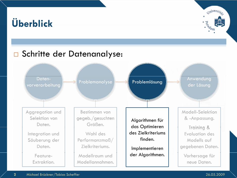
Schritte der Datenanalyse:

Daten-vorverarbeitung

Anwendungder Lösung

Problemanalyse Problemlösung

Aggregation und Selektion von

Daten.

Modell-Selektion& -Anpassung.

Training &

Bestimmen vongegeb./gesuchten

Größen.Algorithmen für das Optimieren

Integration undSäuberung der

Daten.

Training & Evaluation des Modells auf

gegebenen Daten.

Wahl desPerformanzmaß/

Zielkriteriums.

das Optimieren des Zielkriteriums

finden.

Implementieren

26.05.2009Michael Brückner/Tobias Scheffer2

Feature-Extraktion.

Vorhersage für neue Daten.

Modellraum undModellannahmen.

der Algorithmen.

Überwachtes Lernen:

G b T i i d i b k Zi l ib

Problemstellung

Gegeben: Trainingsdaten mit bekannten Zielattributen (gelabelte Daten).Ei b I t (Obj kt B i i l D t kt Eingabe: Instanz (Objekt, Beispiel, Datenpunkt, Merkmalsvektor) = Vektor mit Attribut-Belegungen.

Ausgabe Belegung des/der Zielattribut(e) Ausgabe: Belegung des/der Zielattribut(e). Klassifikation: Nominaler Wertebereich des Zielattributs.

Ordinale Regression: Ordinaler Wertebereich des Zielattributs.

Regression: Numerischer Wertebereich des Zielattributs.

Gesucht: Modell .:f yx


Überwachtes Lernen:

E t h id bä /R l t

Arten von Modellen

Entscheidungsbäume/Regelsysteme: Klassifikations-, Regressions-, Modellbaum.

Lineare Modelle: Lineare Modelle: Trennebenen, Regressionsgerade.

Nicht-lineare Modelle, linear in den Parametern:, Probabilistisches Modell. Nicht-lineare Datentransformation + lineares Modell. Kernel-Modell.

Nicht-lineare Modelle, nicht-linear in den Parametern: Neuronales Netz Neuronales Netz.


Lineare Modelle:

I (V k i Ei ä ) li i

Lineare Modelle für Klassifikation

Instanzen (Vektoren mit m Einträgen) liegen im m-dimensionalen Eingaberaum.Di i d i d h T d (H b H ) Dieser wird in durch Trenngerade (Hyperebene Hw) halbiert.x2x2

Hw +ja nein

x1

-


x1

Lineare Modelle:

I (V k i Ei ä ) li i


Instanzen (Vektoren mit m Einträgen) liegen im m-dimensionalen Eingaberaum.Di i d i d h T d (H b H ) Dieser wird in durch Trenngerade (Hyperebene Hw) halbiert.x2x2

Hw

ID x1 x2 y

1 0,9 3,0 +

x1

2 3,0 4,1 +

3 1,2 0,3 -


x1

Lineare Modelle:

H b i d h N l k d


Hyperebene Hw ist durch Normalenvektor w und Verschiebung w0 gegeben:E t h id f kti ( ) ( ( ))i f

T0| ( ) 0H f w w x x x w

Entscheidungsfunktion:

x2

( ) ( ( ))y sign fx x

x2

Hw

Normalenvektor wZu klassifizierender Punkt zZielfunktionswert f(z)

wz ( )f z

w

w x1

f( )Verschiebung w0


0w

wx1

Lineare Modelle:

U f li i ä li h k


Umformulierung mit zusätzlichem, konstanten Eingabeattribut x0=1: 0

1

ww

w

1

2T0 1 2 0 1 2 2( ) 1m m

m

ww

f w x x x w x x x w

w

x x w

Erweiterte Instanzx2 m

mw x2

HwAus Hyperebene im m-dimensionalen

x1

x0

Aus Hyperebene im m dimensionalen Eingaberaum wird Hyperebene im (m+1)-dimensionalen Eingaberaum.


x1

Lineare Modelle:Lineare Modelle für Regression

Abstand zur Regressionsgerade (Hyperebene Hw) liefert numerischen Wert.

Entscheidungsfunktion:

x2

( ) ( )y fx x

x2

Hw( ) 2f x

ID x1 x2 y

1 0,9 3,0 0,5

x1

( ) 0f x

( ) 1f x

( ) 2f x

( ) 1f x

2 3,0 4,1 2,5

3 1,2 0,3 -1,0


x1( ) 1f x

Lineare Modelle:

Fü kl i h ß Kl ifik i &

Besonders geeignet …

Für kleine – sehr große Klassifikations- & Regressionsprobleme.F ll ht D t li i b Falls unverrauschte Daten linear separierbar.

Falls Interpretierbarkeit der Entscheidung nicht notwendignotwendig.

Für Daten mit überwiegend numerischen Attributen.F ll h ll & i f h V f h ü h Falls schnelles & einfaches Verfahren gewünscht.


Lernen linearer Modelle:

G b T i i i i Zi l ib

Problemstellung

Gegeben: n Trainingsinstanzen xi mit Zielattribut yi.

11 1nx x

X

1 2 1 2

1

n n

m mn

y y yx x

X x x x y

Gesucht: Parametervektor w der Klassifikations-/ Regressionsfunktion .T( )f x x w Maximum Likelihood (ML). Maximum A-Posteriori (MAP).



ML S hä i i i i V l f k i

Ansatz

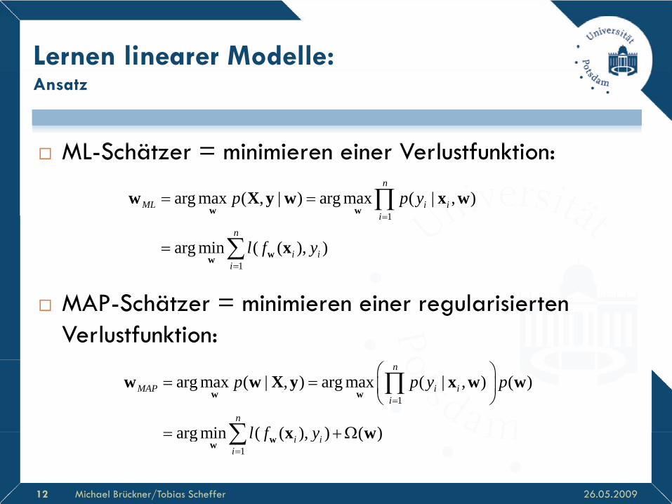
ML-Schätzer = minimieren einer Verlustfunktion:

1

arg max ( , | ) arg max ( | , )n

ML i ii

p p y w ww X y w x w

1

1arg min ( ( ), )

in

i ii

l f y

wwx

MAP-Schätzer = minimieren einer regularisiertenVerlustfunktion:

1

arg max ( | , ) arg max ( | , ) ( )

arg min ( ( ) ) ( )

n

MAP i ii

n

p p y p

l f y

w ww w X y x w w

x w


1arg min ( ( ), ) ( )i i

il f y

wwx w


Bi l

Verlustfunktion für binäre Klassifikation yi {-1,+1}

Binary loss:

0/1

1 ( ) 0( ( ), )

0 ( ) 0i i

i ii i

y fl f y

y f

w

ww

xx

x

( )i isign f yw x l

1

Perceptron loss:

( ) ( ) 0

( ( ) ) 0 ( )i i i iy f y fl f f

w wx x

( )i isign f yw x

( )i iy fw x0 11

Bi l i i h k

Hinge loss:1 ( ) 1 ( ) 0y f y f x x

( ) ( )

( ( ), ) max 0, ( )0 ( ) 0

i i i ip i i i i

i i

y f y fl f y y f

y f

w ww w

w

x xx

Binary loss ist nicht konvex schwer zu minimieren!

Logistic loss:

1 ( ) 1 ( ) 0

( ( ), ) max 0,1 ( )0 1 ( ) 0

i i i ih i i i i

i i

y f y fl f y y f

y f

w w

w ww

x xx x

x


( )log ( ( ), ) log 1 i iy f

i il f y e w xw x


Ab l l

Verlustfunktion für Regression

Absolute loss:( ( ), ) ( )a i i i il f y f y w wx x

l

1

Squared loss: 2( ( ), ) ( )s i i i il f y f y w wx x

( )i if yw x0 11

-Insensitive loss:

( ) ( ) 0( ( ) ) max 0 ( )i i i if y f y

l f y f y

w wx xx x ( ( ), ) max 0, ( )

0 ( ) 0i i i ii i

l f y f yf y

w ww

x xx



Id E h id f d i i ö li h

Regularisierer

Idee: Entscheidung aufgrund so wenig wie möglich Attributen treffen. Wenig Einträge im Parametervektor (Gewichte) ungleich Wenig Einträge im Parametervektor (Gewichte) ungleich

Null: Geringe Manhatten-Norm:

0 0( ) Anzahl 0jw w w 0 ist nicht konvex

schwer zu minimieren!

Geringe (quadratische) euklidische Norm:

1 11

( )m

jj

w

w w

g (q )22

2 21

( )m

jj

w

w w



Zi l Mi i i i i h V l +

Lösen der Minimierungsaufgabe

Ziel: Minimierung von empirischen Verlust + Regularisierer: T

1( ) ( , ) ( )

n

i ii

L l y

w x w w

I.d.R. keine analytische Lösung möglich. Beispiel: Ridge Regression.

Numerische Lösung der primalen OA. Beispiel: Perceptron.

Numerische Lösung der dualen OA. Beispiel: Support Vector Machine (SVM).



G d S h (Ab i i h + Li h)

Numerische Lösungsansätze

Greedy-Suche (Abstiegsrichtung + Linesearch).

AbstiegsrichtungLL(w0)( )

L(w1)

Startlösungww0w1





Greedy-Suche (Abstiegsrichtung + Linesearch). Gradientenabstieg (Newton-Verfahren).

LL(w0)

Gradient

( )

L(w1)

Startlösungww0w1

L(w )





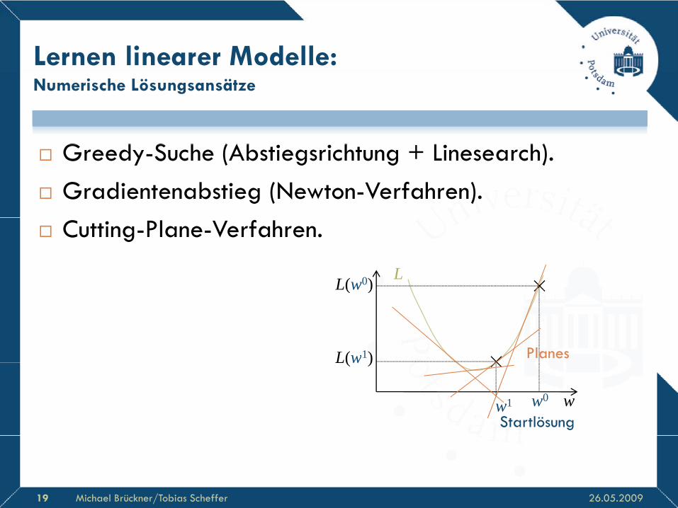
Greedy-Suche (Abstiegsrichtung + Linesearch). Gradientenabstieg (Newton-Verfahren). Cutting-Plane-Verfahren.

LL(w0)

Planes

( )

L(w1)

Startlösungww0w1

L(w )





Greedy-Suche (Abstiegsrichtung + Linesearch). Gradientenabstieg (Newton-Verfahren). Cutting-Plane-Verfahren. Innere-Punkt-Verfahren. LL(w0)( )

L(w1)

Startlösungww0w1

L(w )



V l f k i

Beispiel: Ridge Regression (yi R)

2 Verlustfunktion: Regularisierer:

2T( ( ), )s i i i il f y y w x x w2

21

( )m

jj

w

w2 2n m

Analytische Lösung: 2 2T

1 1

2 2

2 2

( )n m

i i ji j

L y w

w x w

Xw y w

T T

T T T T2

Xw y Xw y w w

w X X I w y Xw y yQuadratische OA ohne

Nebenbedingungen

T T

1T T

( ) 2 2 0L

w X X I w X y

w X X I X yNach w ableiten und Ableitung Null setzen


w X X I X yAbleitung Null setzen

Lernen linearer Modelle:Beispiel: Perceptron (yi {-1,+1})

Verlustfunktion: Regularisierer: .const

T T

T

0( ( ), )

0 0i i i i

p i ii i

y yl f y

y

wx w x w

xx w

Numerische Lösung des primalen Problems:( ) ( ( ), ) .

n

p i iL l f y const ww x

Stochastischer Gradienten- bzw. Subgradientenabstieg.( ( ), )

( )n

p i il f yL

w x

1( ) ( ( ) )p i i

if y

w

G di1

T

T

( )

( ( ), ) 00 0

p i i

i

p i i i i i i

L

l f y y yy

w

w

ww

x x x ww x wi-ter Subgradient

Gradient


0 0i iy w x w



T T

T

0( ( ), )

0 0i i i i

p i ii i

y yl f y

y

wx w x w

xx w

Algorithmus:Perceptron(Instanzen (xi, yi))Setze w = 0DO

( ( ) )n l f y x

WHILE w geändert

1

( ( ), )np i i

i

l f y

w xw w

w

w geä de t

RETURN w




T T

T

0( ( ), )

0 0i i i i

p i ii i

y yl f y

y

wx w x w

xx w


FOR i = 1…n

WHILE w geändert

( ( ), )p i il f y

w x

w ww

w geä de t

RETURN w




T T

T

0( ( ), )

0 0i i i i

p i ii i

y yl f y

y

wx w x w

xx w


FOR i = 1…n

WHILE w geändert

T

T

00 0i i i i

i i

y yy

x x ww w

x ww geä de t

RETURN w




T T

T

0( ( ), )

0 0i i i i

p i ii i

y yl f y

y

wx w x w

xx w


FOR i = 1…nIF THEN

WHILE w geändert

i iy w w x

T 0i iy x w

w geä de t

RETURN w


Lernen linearer Modelle:Beispiel: Support Vector Machine (yi {-1,+1})

Verlustfunktion: Regularisierer:

T T

T

1 1 0( ( ), )

0 1 0i i i i

h i ii i

y yl f y

y

wx w x w

xx w

2

21( )

2

m

jw

w

Numerische Lösung des dualen Problems:12 j

j

1 2 T

1 1

1( ) mit 1 , 02

n m

i j i i i ii j

L w y

w x w

T T T T( ) i 0 0L X X 1

Primales Problem

Duales Problem

Lösen der dualen (quadratischen) OA mittels QP-Solver.

T T T T( ) mit 0, 0 i iL y α α X Xα y α 1 αDuales Problem



G b

Allgemein: Regularized Empirical Risk Minimization

Gegegeben: Konvexe, ableitbare Verlustfunktion l mit Ableitung . Konvexer, ableitbarer Regularisierer mit Ableitung .

( , )l z ylz

Konvexer, ableitbarer Regularisierer mit Ableitung .

Algorithmus:RegERM(Instanzen (xi, yi))

Setze k = 0 0 = 1 w0 = 0

Setze k = 0, 0 = 1, w0 = 0DO

IF k > 0 THEN

T

1( , ) ( )

nk k k

i i ii

l y

g x w x w Barzilai-Borwein-VerfahrenIF k > 0 THEN

1

1

k k k k

k k

w w g

T T1 1 1 1 1k k k k k k k g g g g gVerfahren

WHILE

RETURN wk+1


1k k w w

Zusammenfassung

Li M d ll i fü h ß

Zusammenfassung

Lineare Modelle geeignet für sehr große Klassifikations- & Regressionsprobleme. Besonders geeignet für numerische linear separierbare Daten Besonders geeignet für numerische, linear separierbare Daten.

Lernen von linearen Modellen: Lernen von linearen Modellen: Analytisch (z.B. Ridge Regression). Numerisch (z.B. durch Gradientenabstieg).

Gefundene Lösung global optimal für konvexe Verlustfunktion & Regularisierer.


Date post:	09-Sep-2019
Category:	Documents
Upload:	others
View:	5 times
Download:	0 times

INTELLIGENTE DATENANALYSE IN MATLAB - cs.uni-potsdam.de · Überblick Sh d D lSchritte der...

Documents