42
Intensity Modulated Radiation Therapy Asad Yousuf Medical Physicist Radiation Oncology
| Date post: | 08-Feb-2016 |
| Category: |
Documents |
| Upload: | waqar-ahmed |
| View: | 32 times |
| Download: | 5 times |
Intensity Modulated Radiation Therapy
Asad YousufMedical Physicist
Radiation Oncology
OutlineWhat is IMRTWhat is Inverse Planning
◦Forward planning? Delivery System

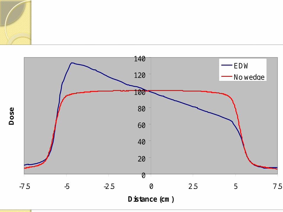
4
0
20
40
60
80
100
120
140
-7.5 -5 -2.5 0 2.5 5 7.5
Distance (cm)
Dos
e
EDWNo wedge

IntroductionAims to deliver radiation more
precisely to the tumor while relatively limiting dose to the surrounding normal tissues.
The purpose of this presentation is to discuss the new concept of IMRT, and its comparison with other RT methods.

Literature Review1950’s the medical linear accelerator was
developed and marketed to treat cancer.1980’s the 3D-Conformal Radiotherapy (3D-CRT)
was introduced.3D-CRT based on 3D dose planning system.Conform the shape of the radiation beam to that
of the tumor.Problem: Cannot conform well to 3D objects due
to the uniformity of beam strength. 30% of tumors exhibit concave features difficult
conventional Conformal RT.

Literature Review1960’s IMRT was first conceptualized 1994 the 1st commercial IMRT delivery
unit was introduced.IMRT An advanced form of 3D-CRT. Based on linear accelerator(L.A.) where
the radiation intensity could be modulated during the treatment.
The field is geometrically shaped by MLC’s.
The intensity is varied pixel-by-pixel within the shaped field.

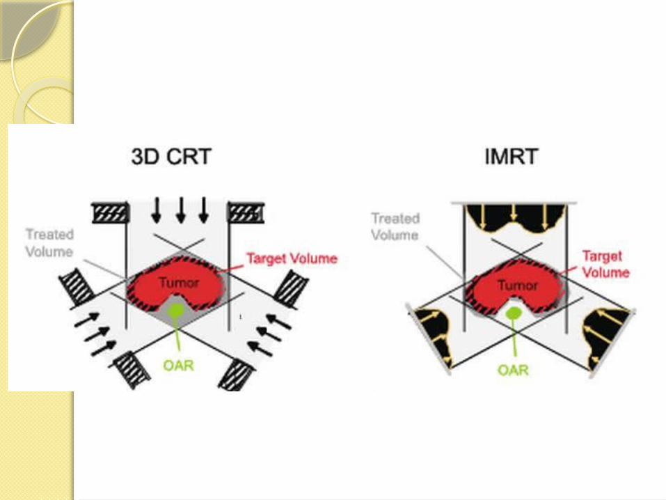
Figure: differences between
(a) conventional radiotherapy,
(b) conformal radiotherapy (CFRT) without intensity-modulation and
(c) CFRT with intensity modulation (IMRT).

Physical AspectIMRT combines two advanced
concepts to deliver 3D CRT:
1. Inverse treatment planning with optimization by computer
2. computer-controlled intensity modulation of the radiation beam during treatment
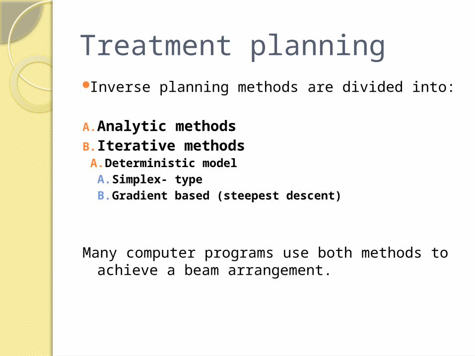
Treatment planning Inverse planning methods are divided into:
A. Analytic methodsB. Iterative methods
A. Deterministic modelA. Simplex- typeB. Gradient based (steepest descent)
Many computer programs use both methods to achieve a beam arrangement.

Analytic methods:
It a mathematical techniques in which the TV dose distribution depends on the point dose intensity.

Iterative methods: It is a manual technique and the
beamlets depends on the cost function that is the energy dose for each point in the TV.
• Gradient Based Method:Two Phases
• Gradient Evaluation• Gradient direction• Gradient Length
• Line search find minimum along the gradient line

Forward Planning

Forward PlanningMethods
◦Planner use a number of open/Wedge/shaped/compensated beams
◦Cross fire at target from varies angles◦Avoids critical organ at same time
Purpose◦Max dose to target/min dose to normal
tissue◦Optimal dose distribution(homogenous
target dose)◦

Forward Planning Flowchart

Features of forward planningEmpirical approachPredictable isodose linesLimited flexibilityDifficult when target
encompasses the OAR

Fluence Map

Work flow

Inverse Planning

Intensity Modulated Fluence Map
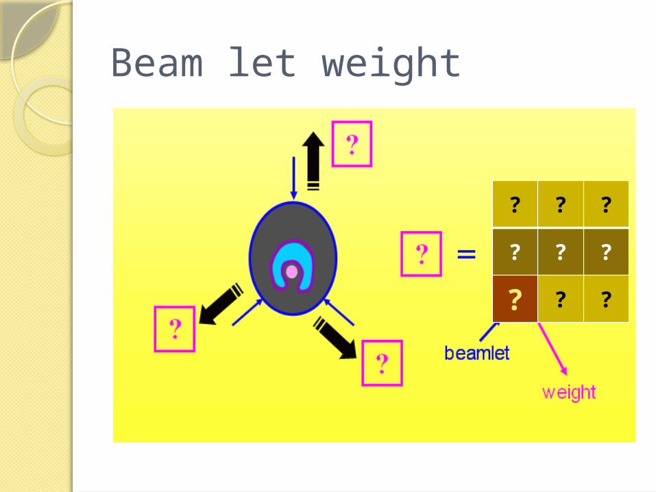
Beam let weight
? ? ?
? ? ?
? ? ?

Inverse Planning ProcessPlanner
◦Specify number & orientation of the open beam
◦Number varies from 5-9 to even 13◦Define objectives (constraints) for the
target & critical organsComputer
◦Iteratively alter the beamlet weight of each beam until the composite 3D distribution satisfies the defined objectives

Constraints vs objectivesObjectives/goal: have clinical
basis e.g. Max dose of spinal cord=45Gy
Constraints/Optimization objectives:
input data in optimizer◦E.g. No dose over 40Gy to spinal
cord◦Extra constraint to shape the DVH◦Do not necessarily reflect a clinical
goal

Optimizationx1 x2 x3
x4 x5 x6
x7 x8 x9
? Achieve costraint
0 0.6 1
0.2 0.9 0.5
0.9 0.8 0
Iteration
ChangeX
No
Yes
Delivered MLC

Goodness of the Treatment
Need to measure how far the objective are achieved
State objectives in mathematical function (OF)
Then measure the value (gradient) of the OFIf OF reaches a minimum indicates a good
plan has been achievedOptimization
Attempt minimize OF by changing x
OF(x)
x

Objective function

Dose/ Dose –Volume based OFFobj(j)
DTarget (D-
P)2
Critical Organ: (D-
Dc)2 if D>Dc
(D-Dc)2
DDc
Fobj(j)

Soft Constraint to target
(D-Dc)2
DDc
(D-Dc)2
D
wi(D-Pi)2
wu(D-Pu)2
Pi Pu
• Soft constraint may also be applied to target as well
• To prevent over-or-under dose to target
• To set a inhomogeneity within target
• More clinically relevant and realistic
Fobj (j) Fobj (j)

Critical organ DVH

PTV DVH

Hard ConstraintAbsolutely not to be violated
under any circumstancesLimit dose to serial structure like?Essentially define allowable
solution space

How to modulate intensity?Compensator MLC’s

Optimal vs Actual fluence
x1 x2 x3
x4 x5 x6
x7 x8 x9
X’1 X’2 X’3
x4 x5 X’6
X’7 X’8 X’9
MLC
Leaf 3A,BLeaf 2A,BLeaf 1A,B

Different MLC modesStep and Shoot
◦Slit beam step across the field◦Beam on whilst the leaves are stationary◦Beam off whilst the leaves are stepping
acrossSliding window mode
◦Slit beam sweeps across the field at various speed generate the required fluence distribution
◦Beam on whilst the leaves are moving


Fluence Map Generation (1)Fluence Map Generation (2)

Fluence Map of one leaf

Fluence Map Generation (All leaf pairs)

Example on whole delivery

Thank You
A smiling face demonstrating how radiation can be deposited
in almost any pattern.


![High-intensity versus low-intensity physical activity or ... · [Intervention Review] High-intensity versus low-intensity physical activity or exercise in people with hip or knee](https://static.documents.pub/doc/80x56/602e37b7b5faa56d200b56dc/high-intensity-versus-low-intensity-physical-activity-or-intervention-review.jpg)