International Global Navigation Satellite Systems Association IGNSS Conference 2016

Colombo Theatres, Kensington Campus, UNSW Australia

6 – 8 December 2016

Inter-Pseudolite Range Augmented GNSS PPP Navigation for Airborne Pseudolite System

Panpan Huang School of Civil and Environmental Engineering,

University of New South Wales, Sydney, NSW 2052, Australia p.huang@student.unsw.edu.au

Chris Rizos School of Civil and Environmental Engineering,

University of New South Wales, Sydney, NSW 2052, Australia c.rizos@unsw.edu.au

Craig Roberts School of Civil and Environmental Engineering,

University of New South Wales, Sydney, NSW 2052, Australia c.roberts@unsw.edu.au

ABSTRACT

Ground-based pseudolite navigation systems have several limitations, such

as low vertical accuracy, susceptibility to multipath effects, and near-far

signal problems. These limitations could be addressed with an airborne

pseudolite system. However, to ensure high user positioning accuracy the

aerial signal transmitters have to be accurately positioned. Commonly used

methods are based on the “inverted GNSS” principle, with ground stations

monitoring the pseudolites, or the differential GNSS (DGNSS) technique

with one or more reference stations. However, the inverted GNSS method

introduces delay for user positioning, while DGNSS has stringent

requirements that include simultaneous measurements made by both the

pseudolite(s) and the reference station(s), and a limitation on the distance

between pseudolite(s) and reference station(s). To address such problems the

authors propose an airborne pseudolite system, consisting of some ground

pseudolites (G-PLs) and airborne pseudolites (A-PLs). The A-PLs in the

proposed system are positioned using the GNSS Precise Point Positioning

(PPP) technique. To enhance the A-PL positioning performance, inter-PL

range measurements could be used as additional observations. The

performance of the proposed system is validated using simulation tests. The

results show that A-PL achieves the best positioning accuracy with

measurements from both G-PLs and limited GNSS satellites or only from G-

PLs where no satellite signals are available.

KEYWORDS: GNSS PPP, Inter-PL range, A-PL positioning, A-PL

trajectory, G-PLs.

1. INTRODUCTION

A pseudolite (PL) navigation system is intended to provide suitably equipped users their

position, velocity, or timing, based on PLs transmitting GPS-like signals. Such systems have

been proposed as a method of GNSS augmentation in signal shaded areas, or as an

independent backup system operated in areas where satellite signals cannot be observed at all

(Kim et al., 2008). One can distinguish between ground-based and airborne pseudolite (G-PL

and A-PL) systems. With the PLs mounted on aircraft, airships, or unmanned aerial vehicles

(UAVs), the A-PL system has advantages compared to the G-PL system, principally because

of reduced near-far problem, lessened multipath disturbance, larger coverage area and better

vertical component observability (Lee et al., 2015).

However, one of the challenges of an A-PL system is determining the precise positions of the

A-PLs in a real-time continuous mode. Tsujii et al. (2001) have proposed three methods for

estimating the A-PL positions: Real-time Kinematic (RTK) & attitude information, the

inverted GPS, and the GPS transceiver method. All of the above can calculate real-time A-PL

positions but need monitoring from ground stations, which can be a challenge. Chandu et al.

(2007) have analysed the effect of movement of the A-PLs and their monitoring time, the

minimum time required to determine the A-PLs’ positions, on the accuracy of user

positioning. The user positioning accuracy is illustrated inversely proportional to the

monitoring time and the movement of the A-PLs. The factors that could cause user position

error also have been identified by García-Crespillo et al. (2015), including the positioning and

timing precision of the A-PLs, effect of A-PL motion, and their ephemeris transmission rate.

To address the problem of the A-PL monitoring time, Lee et al. (2015) have proposed an

airborne relay-based positioning system. This system uses airborne relays to send navigation

signals received from ground reference stations. The user estimates both the airborne relays

and their own position using the RTK technique. However, such a system increases user

position estimation complexity and has reduced performance robustness when one or more

reference stations are not operating for any reason.

In this paper the authors propose an A-PL system consisting of A-PLs and G-PLs. For the

proposed A-PL system, the A-PLs could broadcast their positions to the user in real-time

without monitoring by ground stations. Furthermore, to avoid the problems that might be

brought up by RTK technique, the A-PLs in the proposed system are positioned using GNSS

PPP. As compared with RTK technique, GNSS PPP could deliver comparable positioning

accuracy with lower computational burden, better long-term repeatability, and without the

requirements for nearby reference stations. However, the PPP technique could not be directly

used for A-PL positioning as it requires a comparatively long convergence time to achieve the

desired positioning accuracy as compared with RTK, a relative positioning technique, where

ambiguity resolution (AR) can be more easily achieved. To reduce the convergence time,

there have been many methods proposed to solve the AR in the PPP. However, in this paper it

is proposed that inter-PL range measurements are obtained and combined with satellite

measurements to enhance the performance of GNSS PPP. The advantages of inter-PL range

measurements are investigated. In addition, the impact of factors such as A-PL trajectory, A-

PL positioning error, and the number of G-PLs, were analysed using simulated scenarios.

The paper is organised as follows. In section 2, the configuration of the proposed system is

described. In section 3, the A-PL positioning method based on GNSS PPP combined with

inter-PL ranges is introduced. The simulations of the proposed system are analysed and

results discussed in section 4. Finally, some final remarks are presented.

2. Proposed A-PL System Configuration

For the proposed A-PL system, to get better geometric dilution of precision (GDOP), there are

A-PLs and G-PLs. The G-PLs could also be used for A-PLs’ time synchronisation. The

system configuration is shown in Figure 1. To configure such a system, the following factors

have to be considered: A-PL flying height, A-PL flying trajectory, G-PL distribution, and the

number of A-PLs and G-PLs in use.

Figure 1. Proposed A-PL system configuration

The service coverage area depends on the A-PLs’ flying height. Assume the A-PL flying

height and the minimum elevation angle for users to receive PL signals are h and ,

respectively. Simplifying the Earth to a sphere with radius of R as shown in Figure 2, the

corresponding coverage radius of the A-PL can be calculated as:

cos

cos arcsinR

r RR h

(1)

Figure 2. A-PL system coverage

Table gives some theoretical coverage areas corresponding to different h where is set as

5 .

Table 1. A-PL system coverage with different height

h (km) Coverage (km2)

5 39 10

10 43 10

20 51.2 10

In this paper it is assumed that the A-PLs fly in a circular trajectory at either the same height,

or different heights. To ensure the users within the service coverage area can view at least

four A-PLs, the radius of the A-PLs’ trajectory needs to be as small as possible. However, the

GDOP of the A-PL system must also be taken into consideration when designing the flying

pattern or trajectory, and minimising GDOP demands the trajectory radius be as large as

possible. The maximum radius of the flying trajectory increases as more A-PLs are used.

Similarly, in the case of the G-PLs they are established within the service area and assumed to

be distributed evenly, with a radius configured in the same way as the A-PLs in order to aid

A-PL positioning.

Two scenarios were considered for the A-PL system configuration: where the A-PL has a

clear view of the satellites, and the other PLs include A-PLs and G-PLs, or the scenario where

the A-PL can only receive signals from other PLs, and the satellite signals are blocked or

jammed. To provide high user positioning accuracy, the A-PLs have to be continuously

positioned and broadcast their positions to the users, as described in the following section.

3. A-PL Positioning Method 3.1 GNSS PPP Technique

To realise PPP in a single receiver, rigorous bias models must be developed or the bias

somehow accounted for. For a satellite s observed by receiver r for signal iC on frequency i,

the undifferenced pseudorange and carrier phase observations are commonly modelled as:

, , ,

, , , ,

i i i

i i i i

s s s s s s s

r C r r r i r r C r C

s s s s s s s s

r C r r r i r i r C r C r C

P c dt dt T I B e

L c dt dt T I N b

(2)

where s

r denotes the receiver-satellite geometric range; c is the speed of light; rdt and sdt

are the receiver and satellite clock errors, respectively; s

rT is the slant troposphere delay; s

rI is

the ionospheric delay for a reference frequency; 1

2

2

i

C

i

C

f

f the frequency-dependent coefficient

of the ionosphere; , i

s

r CN is the integer phase ambiguity; , ,i i i

s s

r C r C CB B B is the receiver-

satellite hardware bias for the pseudorange measurement on frequency i; , ,i i i

s s

r C r C Cb b b is

the receiver-satellite uncalibrated phase delays (UPD); i is the wavelength for frequency i;

and , i

s

r Ce and , i

s

r C include measurement noise and multipath of the pseudorange and phase

measurements, respectively. Errors resulting from relativity and phase windup at the satellite

antenna, the antenna phase centre offsets and variations, and site displacement are assumed to

have been corrected and ignored here. The ionospheric delay error can be eliminated using the

ionosphere-free (IF) measurement combination derived from any pair of dual-frequency

measurements (Ge et al., 2008):

1 2

1 21 2

1 2 1 2

2 2

, ,, , 2 2 2 2

C Cs s s

r C r Cr IF C C

C C C C

f f

f f f f

(3)

The tropospheric delay is modelled as a function of the tropospheric zenith hydrostatic and

wet delay (Gao and Shen, 2002):

s s s

r H r H r WT m El Z m El Z (4)

where WZ is the tropospheric zenith wet delay, which is unknown and estimated in the PPP;

while HZ is the tropospheric hydrostatic delay and can be accurately modelled with an

empirical model such as Saastamoinen model, Hopfield model, etc.; and s

H rm El and

s

rm El are the corresponding mapping functions associated with the elevation angle s

rEl of

the receiver to satellite. Precise orbit and clock corrections for the GNSS satellites can be

obtained from International GNSS Service (IGS). The parameters to be estimated are:

r T IFdt Zx r v a N (5)

where x y zr r r r is the receiver position, x y zv v v v is the corresponding

velocity, x y za a a a is the corresponding acceleration, and

1 2

, , ,iss s

IF r IF r IF r IFN N N N denotes the IF receiver-satellite carrier phase ambiguities,

which are preserved as float values during the estimation process. The extended Kalman Filter

(EKF) is used to estimate the unknown parameters. The state model also needs to be

established. The receiver accelerations for kinematic applications are modelled as a first-order

Gauss-Markov (GM) process, while the other parameters are modelled as random walk (RW)

processes. The discrete system model is

1 ,

1 ,

1 ,

, 1 , 1 ,

, 1 , ,

1 ,

1

r

W

k k k k

k k k k

k k k

c

r k r k dt k

W k W k Z k

k k k

T w

T w

Tw

T

dt dt w

Z Z w

w

r

v

a

N

r r v

v v a

a a

N N

(6)

where T and cT are the sampling time and correlation time constant, respectively; k is the

discrete time instant; ,kw is the corresponding white noise.

3.2 GNSS PPP Technique Combined with Inter-PL Range

The inter-PL range measurements are assumed to have a similar form as the GNSS

pseudorange and carrier phase measurements. The inter-PL range observation equations can

be written as:

PP PP P trop PP

PP PP P trop PP PP

P c dt T e

L c dt T N

(7)

where PP is the geometric inter-PL range, which is 2 2 2

P P P

PP x x y y z zr r r r r r

with PL position P P P P

x y zr r r r ; Pdt is the receiver clock error with respect to inter-PL

range measurements; tropT is the tropospheric delay; is the wavelength of the inter-PL

signal; PPN is the carrier phase ambiguity; and PPe and PP are the noises of the

pseudorange and carrier phase measurements, respectively. There are no terms for the

transmitter clock error and ionospheric delay as it is assumed that all the A-PLs are

sequentially time-synchronised to GNSS time, i.e. the transmitter clock error is set as zero,

and the A-PL flying height is less than 50km. The tropospheric delay is estimated using a

tropospheric model such as proposed in (Choudhury et al., 2009). The unknown parameters

are A-PL position and float carrier phase ambiguities, which have the same dynamic models

as used in GNSS PPP.

In the proposed method for combining the inter-PL observations with GNSS PPP, the

measurements from the satellites and observed PLs are assumed independent and processed in

the common EKF with the state and measurement models described above.

The parameter vector is r P T IF PPdt dt Zx r v a N N , and the combined

measurement model can be written as

k k k k z H x v (8)

where kz is the combined measurements from GNSS and inter-PL ranges; kv is the

measurement noise; the design matrix kH of only carrier-phase based measurements can be

written as:

1 1

2 2

1

2

,

,

6 1

,

,

,

6 1 1

,

1

1

1

1

1

1

m m

n

s s

r k r

s s

r k r

m m m m m n

s s

r k rk

P

r k

P

r k

n n n n m n n

P

r k

m El

m El

m El

e

e

0 0 I 0

eH

e

e

0 0 0 0 I

e

(9)

where e is the line-of-sight vector between the PL and satellite/PL.

4. Simulation Results and Analysis 4.1 Simulation Assumptions

To investigate the influence of inter-PL ranges on A-PL positioning using the GNSS PPP

technique, the simulations for the two scenarios described earlier were carried out. In the

simulations, the A-PLs were assumed to constantly fly a circular trajectory at the same height,

referred to as uninclined trajectory, or two different inclined trajectories with the same centre.

The A-PLs on the same circular trajectory are distributed with equal fixed distance from each

other, with one fixed at the centre of circular trajectory in order to improve the positioning

geometry as shown in Figure 3. The flying height was set to 10km for the uninclined

trajectory in the following simulations. The radius of the coverage area with minimum

elevation angle 5 was 104km. To ensure at least four LOS to A-PLs in the case of the users

and to enable good GDOP conditions, seven A-PLs were used in the simulation. The radius of

the A-PLs’ flying trajectory was set as 50km. The impact of A-PL trajectory inclination,

observed A-PL positioning error and the number of G-PLs was investigated.

2.542.55

2.562.57

2.582.59

x 106

2.54

2.56

2.58

2.6

x 106

2.54

2.55

2.56

2.57

2.58

2.59

x 106

A-PL Flying Oribt

2.54

2.56

2.58

2.6

x 106

2.54

2.56

2.58

2.6

x 106

2.55

2.56

2.57

2.58

2.59

2.6

x 106

A-PL Flying Oribt

(a) Uninclined trajectory (b) Inclined trajectory

Figure 3. A-PL trajectory scenarios

4.2 A-PL Positioning Performance

Only the comparison of A-PL positioning performance using measurements from a limited

number of GNSS satellites and the observed A-PLs is presented. One of the A-PLs on the

circular trajectory is chosen to analyse the positioning results. Figure 4 shows the comparison

A-PL positioning results with different types of measurements. It can be seen that GNSS PPP

with synchronised A-PLs has the fastest convergence speed compared with the GNSS PPP

alone or GNSS PPP with unsynchronised A-PLs, which means the observed A-PLs have large

position errors.

0 500 1000 1500 2000 25000

1

2

3

4

5

6

7

Time (s)

Positio

n E

rror

(m)

A-PL Positioning Comparison

GNSS PPP

GNSS PPP with Synchronised A-PLs

GNSS PPP with Unsynchronised A-PLs

Figure 4. A-PL positioning accuracy with different types of measurements

From Figure 4 and Table 2 one can see that A-PL positioning based on GNSS PPP is better

than that with measurements from GNSS and unsynchronised A-PLs, but worse than that with

measurements from GNSS PPP and synchronised A-PLs. This is because the observed A-PL

positioning errors have a significant influence on the results, as discussed in the following

section.

Table 2. A-PL positioning accuracy with different types of measurements

Methods Positioning Errors (m)

East North Up

GNSS PPP 0.057 0.163 0.071

With Synchronized A-PL 0.025 0.053 0.054

With unsynchronised A-PL 0.232 0.186 0.311

4.3 Impact Factors Analysis

The impact factors are analysed in terms of A-PL positioning accuracy for the two scenarios

referred to earlier. During the simulations, all the observed A-PL positions are assumed

known from the results of GNSS PPP.

4.3.1 A-PL Trajectory Inclination

To improve the A-PL geometry, the A-PLs were assumed to fly in an inclined trajectory

relative the local horizontal plane (see Figure 3b). To compare with the uninclined trajectory

scenario, the same number of A-PLs, seven A-PLs with one at the centre, were used but on

two different trajectories. Three of the A-PLs were on one trajectory with an inclined angle ,

the other three on the other trajectory with as in Figure 3b to improve GDOP. The

performance of the system with various trajectory inclinations was evaluated for the second

scenario where no satellite signals were available. To be able to design the inclined trajectory,

the minimum A-PL flying height was assumed to be 1km. The noises for the simulated

different inclined degrees are randomly added. Five G-PLs were assumed to be able to be

observed by the A-PLs. They were distributed in the same way as the A-PLs, with one fixed

at the centre right below the centred A-PL and the other four evenly distributed around. The

initial positions of the A-PLs were derived from the GNSS positioning results.

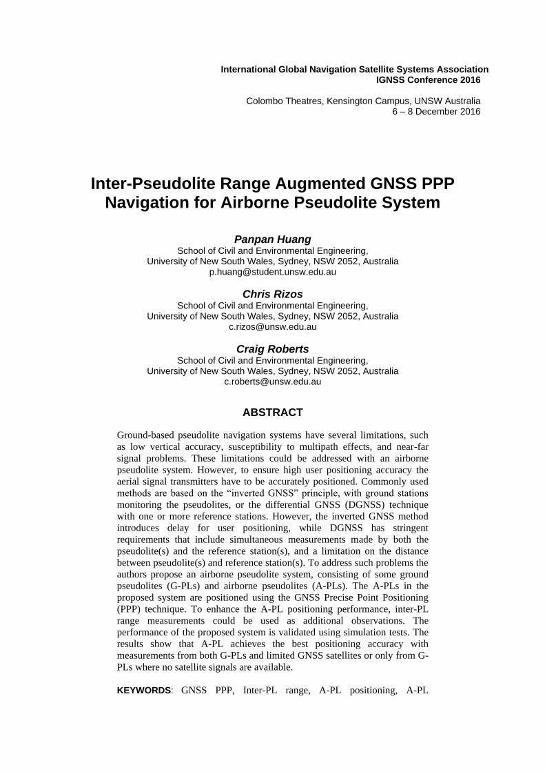
Table 3. A-PL positioning errors with different inclinations

Inclination (°)

A-PL Positioning Error （m）

Observation only from G-PLs Observation from both G-PLs and A-

PLs

East North Up East North Up

0 0.029 0.114 0.237 0.308 0.146 0.144

15 0.127 0.101 0.234 0.563 0.333 0.118

30 0.118 0.106 0.233 0.383 0.186 0.164

45 0.074 0.104 0.179 0.285 0.177 0.119

60 0.053 0.111 0.178 0.212 0.216 0.134

75 0.030 0.104 0.267 0.344 0.197 0.196

Table 3 shows the A-PL positioning accuracy after convergence which is defined as 30 cm for

the magnitude error. It can be seen from Table 3 that A-PL positioning accuracy was better

for any inclination angle when it only uses observations from the G-PLs instead of from both

the A-PLs and G-PLs where the observed A-PLs are unsynchronised. Figure 5 shows the

comparison of A-PL positioning results with varying inclined trajectories, where the

observations are only from the G-PLs. The A-PL positioning accuracies for different

inclination angle are essentially the same after the solutions converge. The accuracy of the

initial position constrains the final Up component positioning accuracy. The A-PL cannot

estimate its 3D positions with observations only from the G-PLs, all of which are located at

the same height. To further improve the Up component accuracy, height (or height difference)

measurements from altimeter can be added in practice.

0 500 1000 1500 2000 2500 3000 3500 40000

20

40

60

80

100

120

140

160

180

Time (s)

Po

sitio

n E

rro

r (m

)

A-PL Positioning Accuracy with Observation only from G-PLs

Inclination 0 Degree

Inclination 15 Degree

Inclination 30 Degree

Inclination 45 Degree

Inclination 60 Degree

Inclination 75 Degree

Figure 5. Comparison of A-PL positioning accuracy with different inclinations

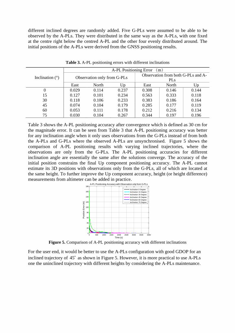
For the user end, it would be better to use the A-PLs configuration with good GDOP for an

inclined trajectory of 45 as shown in Figure 5. However, it is more practical to use A-PLs

one the uninclined trajectory with different heights by considering the A-PLs maintenance.

0 500 1000 1500 2000 2500 3000 3500 40001.05

1.1

1.15

1.2

1.25

1.3

Time (s)

GD

OP

A-PL GDOP

Inclination 0 Degree

Inclination 15 Degree

Inclination 30 Degree

Inclination 45 Degree

Inclination 60 Degree

Inclination 75 Degree

Figure 6. A-PL GDOP variation with different inclinations

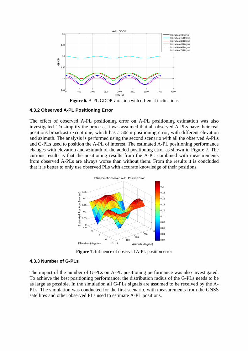
4.3.2 Observed A-PL Positioning Error

The effect of observed A-PL positioning error on A-PL positioning estimation was also

investigated. To simplify the process, it was assumed that all observed A-PLs have their real

positions broadcast except one, which has a 50cm positioning error, with different elevation

and azimuth. The analysis is performed using the second scenario with all the observed A-PLs

and G-PLs used to position the A-PL of interest. The estimated A-PL positioning performance

changes with elevation and azimuth of the added positioning error as shown in Figure 7. The

curious results is that the positioning results from the A-PL combined with measurements

from observed A-PLs are always worse than without them. From the results it is concluded

that it is better to only use observed PLs with accurate knowledge of their positions.

0

100

200

300

400

-100

-50

0

50

1000

0.05

0.1

0.15

0.2

0.25

Azimuth (degree)

Influence of Observed A-PL Position Error

Elevation (degree)

Estim

ate

d P

ositio

n E

rro

r (m

)

0.02

0.04

0.06

0.08

0.1

0.12

0.14

0.16

0.18

0.2

Figure 7. Influence of observed A-PL position error

4.3.3 Number of G-PLs

The impact of the number of G-PLs on A-PL positioning performance was also investigated.

To achieve the best positioning performance, the distribution radius of the G-PLs needs to be

as large as possible. In the simulation all G-PLs signals are assumed to be received by the A-

PLs. The simulation was conducted for the first scenario, with measurements from the GNSS

satellites and other observed PLs used to estimate A-PL positions.

5 10 15 20 25 30 35

0.03

0.035

0.04

0.045

0.05

0.055

0.06

0.065

0.07

0.075

0.08

Influence of Different Number of G-PLs

Number of G-PLsP

ositio

n E

rro

r

Figure 8. A-PL positioning results with different number of G-PLs

Table 4. A-PL positioning eerrors with different number of G-PLs

Number A-PL Positioning Error

(m）

East North Up

4 0.014 0.016 0.040

5 0.011 0.013 0.035

6 0.010 0.012 0.032

7 0.009 0.011 0.032

8 0.009 0.009 0.026

9 0.009 0.009 0.024

Figure 8 and Table 4 illustrate the A-PL positioning performance with different numbers of

observed G-PLs. It is clearly seen that the A-PL positioning accuracy gradually improves with

an increase in the number of G-PLs, especially for the horizontal components. In practice, 6-

10 G-PLs would be sufficient to provide the necessary enhancement for A-PL positioning.

5. Concluding Remarks

In a standard A-PL system, the A-PL positioning based on the inverted GNSS method or

DGNSS suffers from delay for monitoring the A-PLs, or the requirement for ground reference

stations. In this paper an A-PL system based on the GNSS PPP technique has been proposed.

Its configuration and A-PL positioning, combined with inter-PL range between the A-PL and

other PLs, are investigated. Simulations have been performed to compare A-PL positioning

performance using different measurements, and to analyse the impact of different variable

factors for two different scenarios on the proposed airborne PL system. The simulation results

demonstrate that the best A-PL positioning performances are based on measurements from

both G-PLs and limited GNSS satellites for the first scenario and only from G-PLs for the

second scenario when the observed A-PLs’ positions are not accurately known.

ACKNOWLEDGEMENTS

This study is supported by Chinese Scholarship Council (CSC) awarded to the first author.

REFERENCES

Chandu, B., Pant, R., & Moudgalya, K. (2007). Modeling and simulation of a precision navigation

system using pseudolites mounted on airships Proceedings of the 7th Aviation Technology,

Integration, and Operations (ATIO) Conferences, Belfast, Northern Ireland, 18-20.

Choudhury, M., Harvey, B., & Rizos, C. (2009). Tropospheric correction for Locata when known

point ambiguity resolution technique is used in static survey, IGNSS Symp.

Gao, Y., & Shen, X. (2002). A New Method for Carrier‐Phase‐Based Precise Point Positioning.

Navigation, 49(2): 109-116.

García-Crespillo, O., Nossek, E., Winterstein, A., Belabbas, B., & Meurer, M. (2015). Use of High

Altitude Platform Systems to augment ground based APNT systems 2015 IEEE/AIAA 34th

Digital Avionics Systems Conference (DASC), 2A3-1-2A3-9.

Ge, M., Gendt, G., Rothacher, M. A., Shi, C., & Liu, J. (2008). Resolution of GPS carrier-phase

ambiguities in precise point positioning (PPP) with daily observations. Journal of Geodesy,

82(7): 389-399.

Kim, D., Park, B., Lee, S., Cho, A., Kim, J., & Kee, C. (2008). Design of efficient navigation message

format for UAV pseudolite navigation system. IEEE Transactions on Aerospace and

Electronic Systems, 44(4): 1342-1355.

Lee, K., Noh, H., & Lim, J. (2015). Airborne relay-based regional positioning system. Sensors, 15(6):

12682-12699.

Tsujii, T., Rizos, C., Wang, J., Dai, L., Roberts, C., & Harigae, M. (2001). A navigation/positioning

service based on pseudolites installed on stratospheric airships 5th Int. Symp. on Satellite

Navigation Technology & Applications, 24-27.