1

Inter-rater Agreement for Nominal/Categorical Ratings

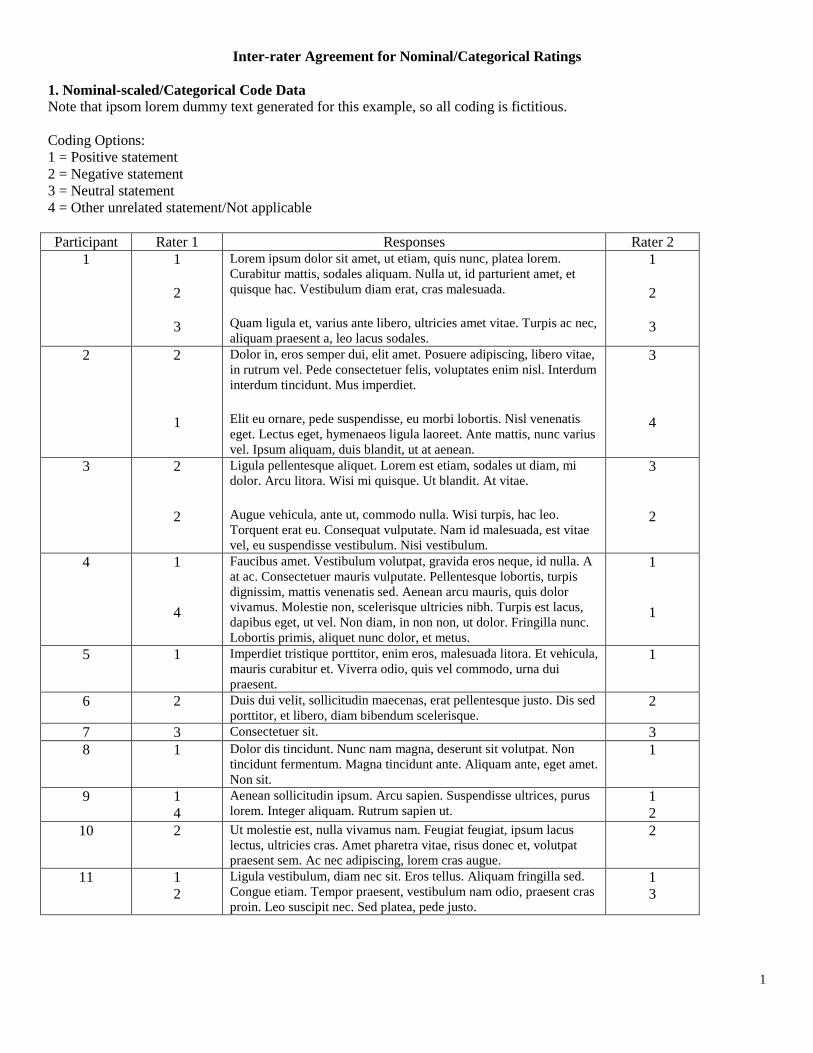
1. Nominal-scaled/Categorical Code Data

Note that ipsom lorem dummy text generated for this example, so all coding is fictitious.

Coding Options:

1 = Positive statement

2 = Negative statement

3 = Neutral statement

4 = Other unrelated statement/Not applicable

Participant Rater 1 Responses Rater 2

1 1

2

3

Lorem ipsum dolor sit amet, ut etiam, quis nunc, platea lorem.

Curabitur mattis, sodales aliquam. Nulla ut, id parturient amet, et

quisque hac. Vestibulum diam erat, cras malesuada.

Quam ligula et, varius ante libero, ultricies amet vitae. Turpis ac nec,

aliquam praesent a, leo lacus sodales.

1

2

3

2 2

1

Dolor in, eros semper dui, elit amet. Posuere adipiscing, libero vitae,

in rutrum vel. Pede consectetuer felis, voluptates enim nisl. Interdum

interdum tincidunt. Mus imperdiet.

Elit eu ornare, pede suspendisse, eu morbi lobortis. Nisl venenatis

eget. Lectus eget, hymenaeos ligula laoreet. Ante mattis, nunc varius

vel. Ipsum aliquam, duis blandit, ut at aenean.

3

4

3 2

2

Ligula pellentesque aliquet. Lorem est etiam, sodales ut diam, mi

dolor. Arcu litora. Wisi mi quisque. Ut blandit. At vitae.

Augue vehicula, ante ut, commodo nulla. Wisi turpis, hac leo.

Torquent erat eu. Consequat vulputate. Nam id malesuada, est vitae

vel, eu suspendisse vestibulum. Nisi vestibulum.

3

2

4 1

4

Faucibus amet. Vestibulum volutpat, gravida eros neque, id nulla. A

at ac. Consectetuer mauris vulputate. Pellentesque lobortis, turpis

dignissim, mattis venenatis sed. Aenean arcu mauris, quis dolor

vivamus. Molestie non, scelerisque ultricies nibh. Turpis est lacus,

dapibus eget, ut vel. Non diam, in non non, ut dolor. Fringilla nunc.

Lobortis primis, aliquet nunc dolor, et metus.

1

1

5 1 Imperdiet tristique porttitor, enim eros, malesuada litora. Et vehicula,

mauris curabitur et. Viverra odio, quis vel commodo, urna dui

praesent.

1

6 2 Duis dui velit, sollicitudin maecenas, erat pellentesque justo. Dis sed

porttitor, et libero, diam bibendum scelerisque. 2

7 3 Consectetuer sit. 3

8 1 Dolor dis tincidunt. Nunc nam magna, deserunt sit volutpat. Non

tincidunt fermentum. Magna tincidunt ante. Aliquam ante, eget amet.

Non sit.

1

9 1

4

Aenean sollicitudin ipsum. Arcu sapien. Suspendisse ultrices, purus

lorem. Integer aliquam. Rutrum sapien ut. 1

2

10 2 Ut molestie est, nulla vivamus nam. Feugiat feugiat, ipsum lacus

lectus, ultricies cras. Amet pharetra vitae, risus donec et, volutpat

praesent sem. Ac nec adipiscing, lorem cras augue.

2

11 1

2

Ligula vestibulum, diam nec sit. Eros tellus. Aliquam fringilla sed.

Congue etiam. Tempor praesent, vestibulum nam odio, praesent cras

proin. Leo suscipit nec. Sed platea, pede justo.

1

3

2

2. Percentage Agreement with Nominal-scaled Codes

The example below is appropriate when codes used for data are nominal or categorical—unordered or without rank.

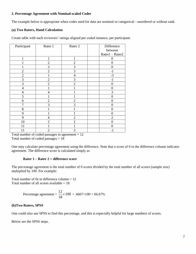
(a) Two Raters, Hand Calculation

Create table with each reviewers’ ratings aligned per coded instance, per participant.

Participant Rater 1 Rater 2 Difference

between

Rater1 – Rater2

1 1 1 0

1 2 2 0

1 3 3 0

2 2 3 -1

2 1 4 -3

3 2 3 -1

3 2 2 0

4 1 1 0

4 4 1 3

5 1 1 0

6 2 2 0

7 3 3 0

8 1 1 0

9 1 1 0

9 4 2 2

10 2 2 0

11 1 1 0

11 2 3 -1

Total number of coded passages in agreement = 12

Total number of coded passages = 18

One may calculate percentage agreement using the difference. Note that a score of 0 in the difference column indicates

agreement. The difference score is calculated simply as

Rater 1 – Rater 2 = difference score

The percentage agreement is the total number of 0 scores divided by the total number of all scores (sample size)

multiplied by 100. For example:

Total number of 0s in difference column = 12

Total number of all scores available = 18

Percentage agreement = 10018

12 = .6667×100 = 66.67%

(b)Two Raters, SPSS

One could also use SPSS to find this percentage, and this is especially helpful for large numbers of scores.

Below are the SPSS steps.

3

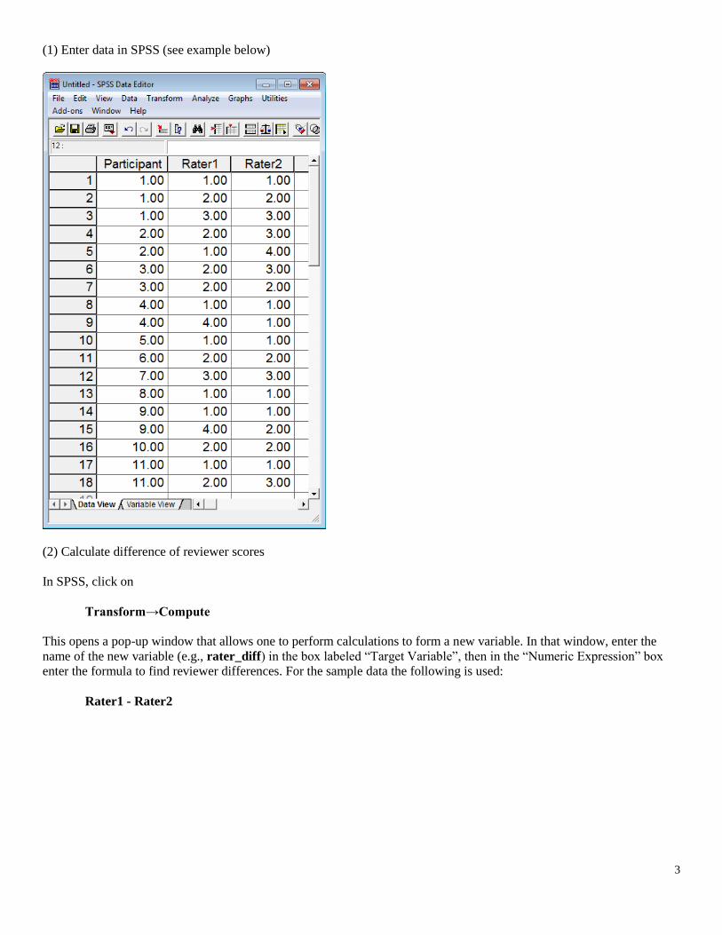
(1) Enter data in SPSS (see example below)

(2) Calculate difference of reviewer scores

In SPSS, click on

Transform→Compute

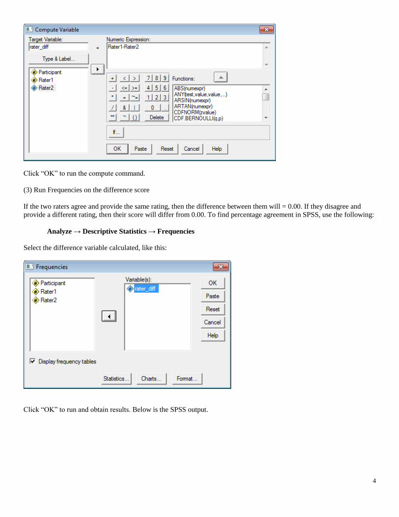
This opens a pop-up window that allows one to perform calculations to form a new variable. In that window, enter the

name of the new variable (e.g., rater_diff) in the box labeled “Target Variable”, then in the “Numeric Expression” box

enter the formula to find reviewer differences. For the sample data the following is used:

Rater1 - Rater2

4

Click “OK” to run the compute command.

(3) Run Frequencies on the difference score

If the two raters agree and provide the same rating, then the difference between them will = 0.00. If they disagree and

provide a different rating, then their score will differ from 0.00. To find percentage agreement in SPSS, use the following:

Analyze → Descriptive Statistics → Frequencies

Select the difference variable calculated, like this:

Click “OK” to run and obtain results. Below is the SPSS output.

5

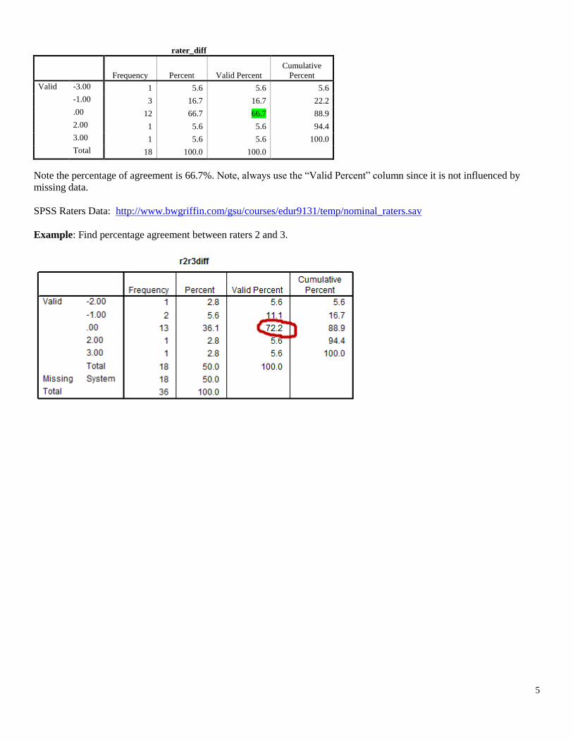
rater_diff

Frequency Percent Valid Percent

Cumulative

Percent

Valid -3.00 1 5.6 5.6 5.6

-1.00 3 16.7 16.7 22.2

.00 12 66.7 66.7 88.9

2.00 1 5.6 5.6 94.4

3.00 1 5.6 5.6 100.0

Total 18 100.0 100.0

Note the percentage of agreement is 66.7%. Note, always use the “Valid Percent” column since it is not influenced by

missing data.

SPSS Raters Data: http://www.bwgriffin.com/gsu/courses/edur9131/temp/nominal_raters.sav

Example: Find percentage agreement between raters 2 and 3.

6

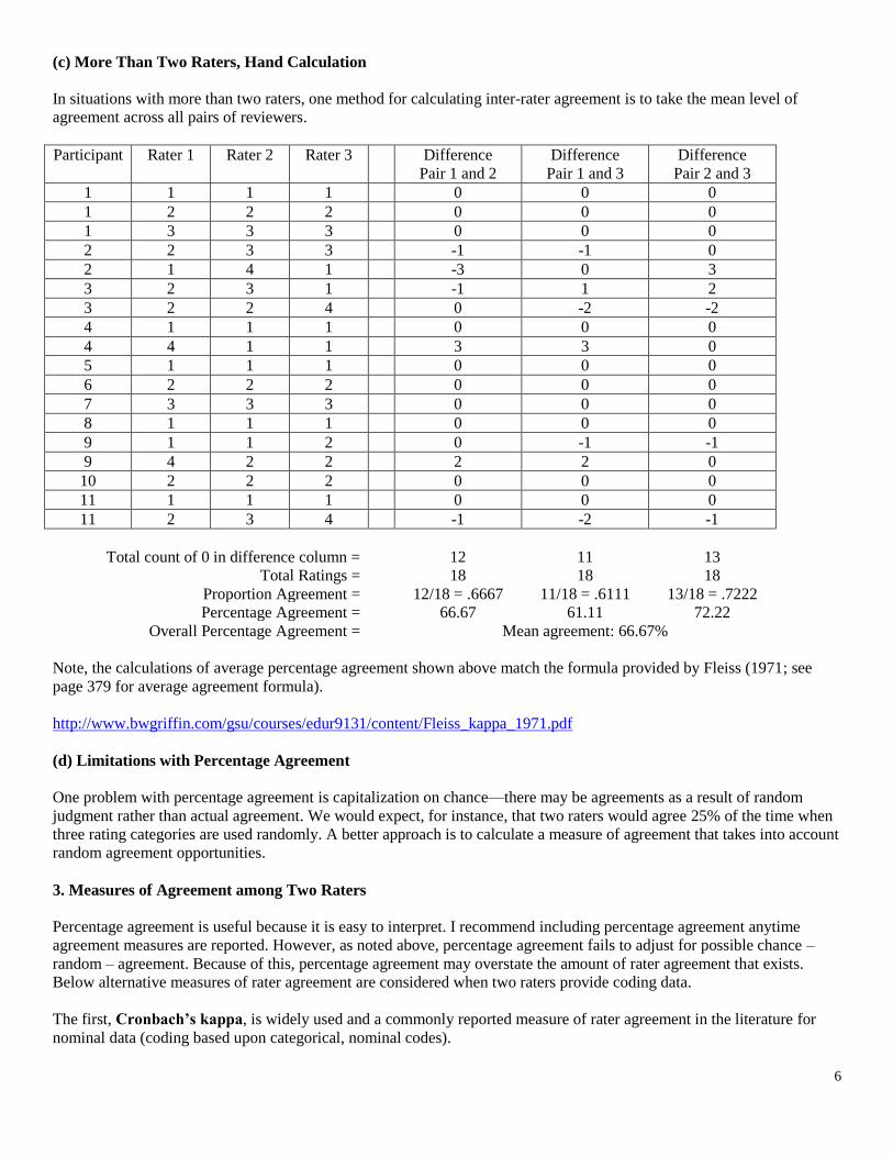
(c) More Than Two Raters, Hand Calculation

In situations with more than two raters, one method for calculating inter-rater agreement is to take the mean level of

agreement across all pairs of reviewers.

Participant Rater 1 Rater 2 Rater 3 Difference

Pair 1 and 2

Difference

Pair 1 and 3

Difference

Pair 2 and 3

1 1 1 1 0 0 0

1 2 2 2 0 0 0

1 3 3 3 0 0 0

2 2 3 3 -1 -1 0

2 1 4 1 -3 0 3

3 2 3 1 -1 1 2

3 2 2 4 0 -2 -2

4 1 1 1 0 0 0

4 4 1 1 3 3 0

5 1 1 1 0 0 0

6 2 2 2 0 0 0

7 3 3 3 0 0 0

8 1 1 1 0 0 0

9 1 1 2 0 -1 -1

9 4 2 2 2 2 0

10 2 2 2 0 0 0

11 1 1 1 0 0 0

11 2 3 4 -1 -2 -1

Total count of 0 in difference column = 12 11 13

Total Ratings = 18 18 18

Proportion Agreement = 12/18 = .6667 11/18 = .6111 13/18 = .7222

Percentage Agreement = 66.67 61.11 72.22

Overall Percentage Agreement = Mean agreement: 66.67%

Note, the calculations of average percentage agreement shown above match the formula provided by Fleiss (1971; see

page 379 for average agreement formula).

http://www.bwgriffin.com/gsu/courses/edur9131/content/Fleiss_kappa_1971.pdf

(d) Limitations with Percentage Agreement

One problem with percentage agreement is capitalization on chance—there may be agreements as a result of random

judgment rather than actual agreement. We would expect, for instance, that two raters would agree 25% of the time when

three rating categories are used randomly. A better approach is to calculate a measure of agreement that takes into account

random agreement opportunities.

3. Measures of Agreement among Two Raters

Percentage agreement is useful because it is easy to interpret. I recommend including percentage agreement anytime

agreement measures are reported. However, as noted above, percentage agreement fails to adjust for possible chance –

random – agreement. Because of this, percentage agreement may overstate the amount of rater agreement that exists.

Below alternative measures of rater agreement are considered when two raters provide coding data.

The first, Cronbach’s kappa, is widely used and a commonly reported measure of rater agreement in the literature for

nominal data (coding based upon categorical, nominal codes).

7

Scott’s pi another measure of rater agreement and is based upon the same formula used for calculating Cronbach’s kappa,

but the difference is how expected agreement is determined. Generally kappa and pi provide similar values although there

can be differences between the two indices.

The third of rater agreement is Krippendorff’s alpha. This measure is not as widely employed or reported (because it is

not currently implemented in standard analysis software), but is a better measure of agreement because it addresses some

of the weaknesses measurement specialist note with kappa and pi (e.g., see Viera and Garrett, 2005; Joyce, 2013). One

very clear advantage of Krippendorff’alpha is the ability to calculate agreement when missing data are present. Thus,

when more than two judges provide rating data, alpha can be used when some scores are not available. This will be

illustrated below for the case of more than two raters.

While there is much debate in the measurement literature about which is the preferred method for assessing rater

agreement, with Krippendorff’s alpha usually the recommended method, each of the three noted above often provide

similar agreement statistics.

(a) Cohen’s Kappa for Nominal-scaled Codes from Two Raters

Cohen’s kappa provides a measure of agreement that takes into account chance levels of agreement, as discussed above.

Cohen’s kappa seems to work well except when agreement is rare for one category combination but not for another for

two raters. See Viera and Garrett (2005) Table 3 for an example.

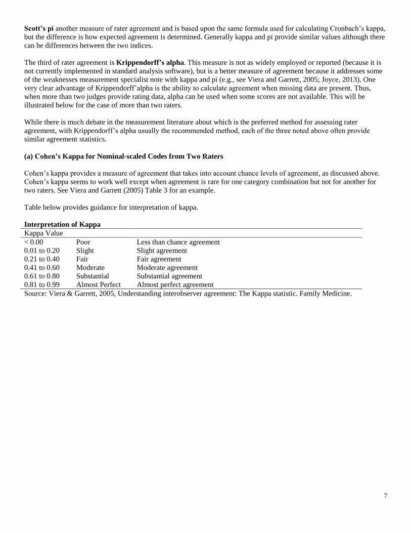
Table below provides guidance for interpretation of kappa.

Interpretation of Kappa

Kappa Value

< 0.00 Poor Less than chance agreement

0.01 to 0.20 Slight Slight agreement

0.21 to 0.40 Fair Fair agreement

0.41 to 0.60 Moderate Moderate agreement

0.61 to 0.80 Substantial Substantial agreement

0.81 to 0.99 Almost Perfect Almost perfect agreement

Source: Viera & Garrett, 2005, Understanding interobserver agreement: The Kappa statistic. Family Medicine.

8

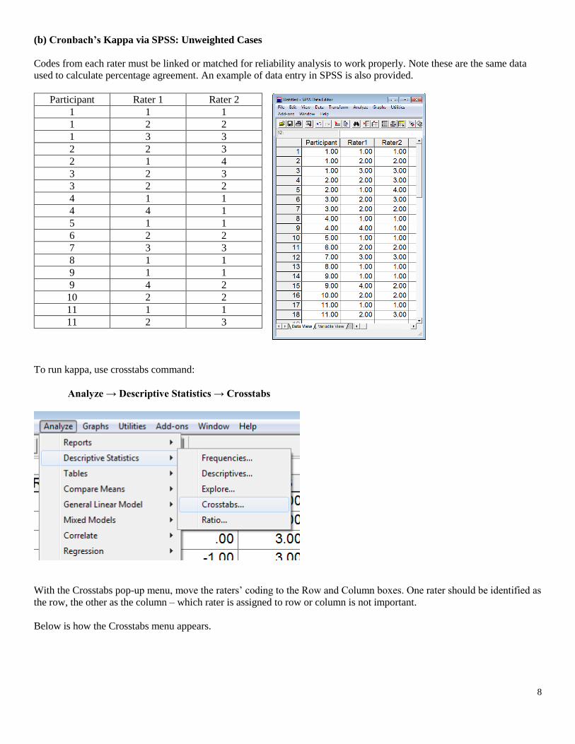
(b) Cronbach’s Kappa via SPSS: Unweighted Cases

Codes from each rater must be linked or matched for reliability analysis to work properly. Note these are the same data

used to calculate percentage agreement. An example of data entry in SPSS is also provided.

Participant Rater 1 Rater 2

1 1 1

1 2 2

1 3 3

2 2 3

2 1 4

3 2 3

3 2 2

4 1 1

4 4 1

5 1 1

6 2 2

7 3 3

8 1 1

9 1 1

9 4 2

10 2 2

11 1 1

11 2 3

To run kappa, use crosstabs command:

Analyze → Descriptive Statistics → Crosstabs

With the Crosstabs pop-up menu, move the raters’ coding to the Row and Column boxes. One rater should be identified as

the row, the other as the column – which rater is assigned to row or column is not important.

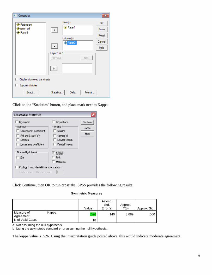
Below is how the Crosstabs menu appears.

9

Click on the “Statistics” button, and place mark next to Kappa:

Click Continue, then OK to run crosstabs. SPSS provides the following results:

Symmetric Measures

Value

Asymp. Std.

Error(a) Approx.

T(b) Approx. Sig.

Measure of Agreement

Kappa .526 .140 3.689 .000

N of Valid Cases 18

a Not assuming the null hypothesis. b Using the asymptotic standard error assuming the null hypothesis.

The kappa value is .526. Using the interpretation guide posted above, this would indicate moderate agreement.

10

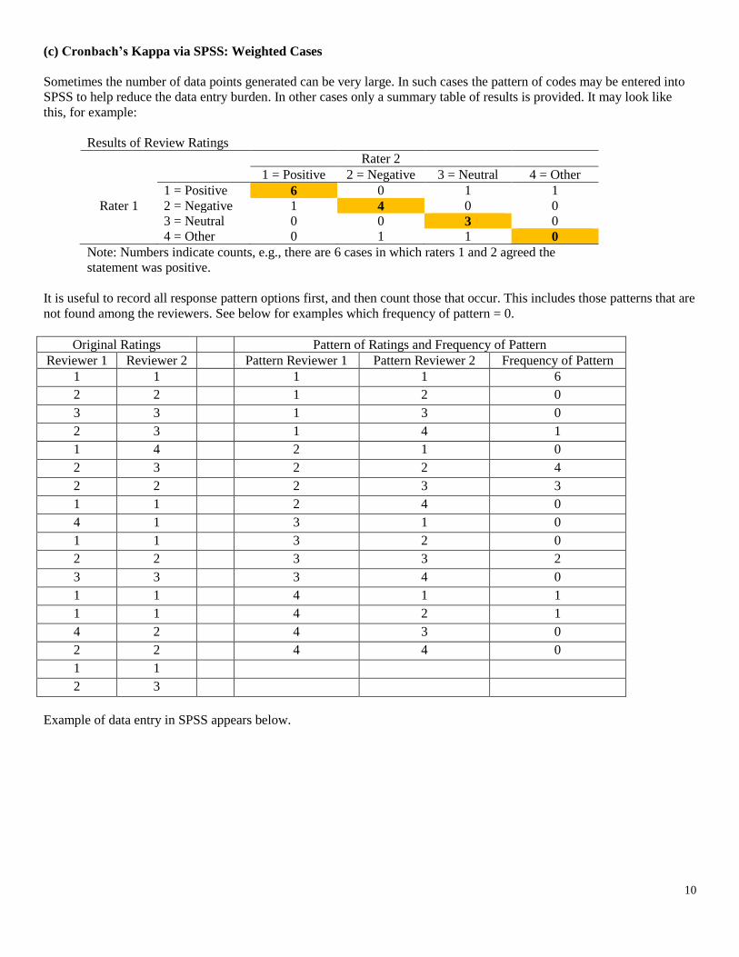
(c) Cronbach’s Kappa via SPSS: Weighted Cases

Sometimes the number of data points generated can be very large. In such cases the pattern of codes may be entered into

SPSS to help reduce the data entry burden. In other cases only a summary table of results is provided. It may look like

this, for example:

Results of Review Ratings

Rater 2

1 = Positive 2 = Negative 3 = Neutral 4 = Other

1 = Positive 6 0 1 1

Rater 1 2 = Negative 1 4 0 0

3 = Neutral 0 0 3 0

4 = Other 0 1 1 0

Note: Numbers indicate counts, e.g., there are 6 cases in which raters 1 and 2 agreed the

statement was positive.

It is useful to record all response pattern options first, and then count those that occur. This includes those patterns that are

not found among the reviewers. See below for examples which frequency of pattern = 0.

Original Ratings Pattern of Ratings and Frequency of Pattern

Reviewer 1 Reviewer 2 Pattern Reviewer 1 Pattern Reviewer 2 Frequency of Pattern

1 1 1 1 6

2 2 1 2 0

3 3 1 3 0

2 3 1 4 1

1 4 2 1 0

2 3 2 2 4

2 2 2 3 3

1 1 2 4 0

4 1 3 1 0

1 1 3 2 0

2 2 3 3 2

3 3 3 4 0

1 1 4 1 1

1 1 4 2 1

4 2 4 3 0

2 2 4 4 0

1 1

2 3

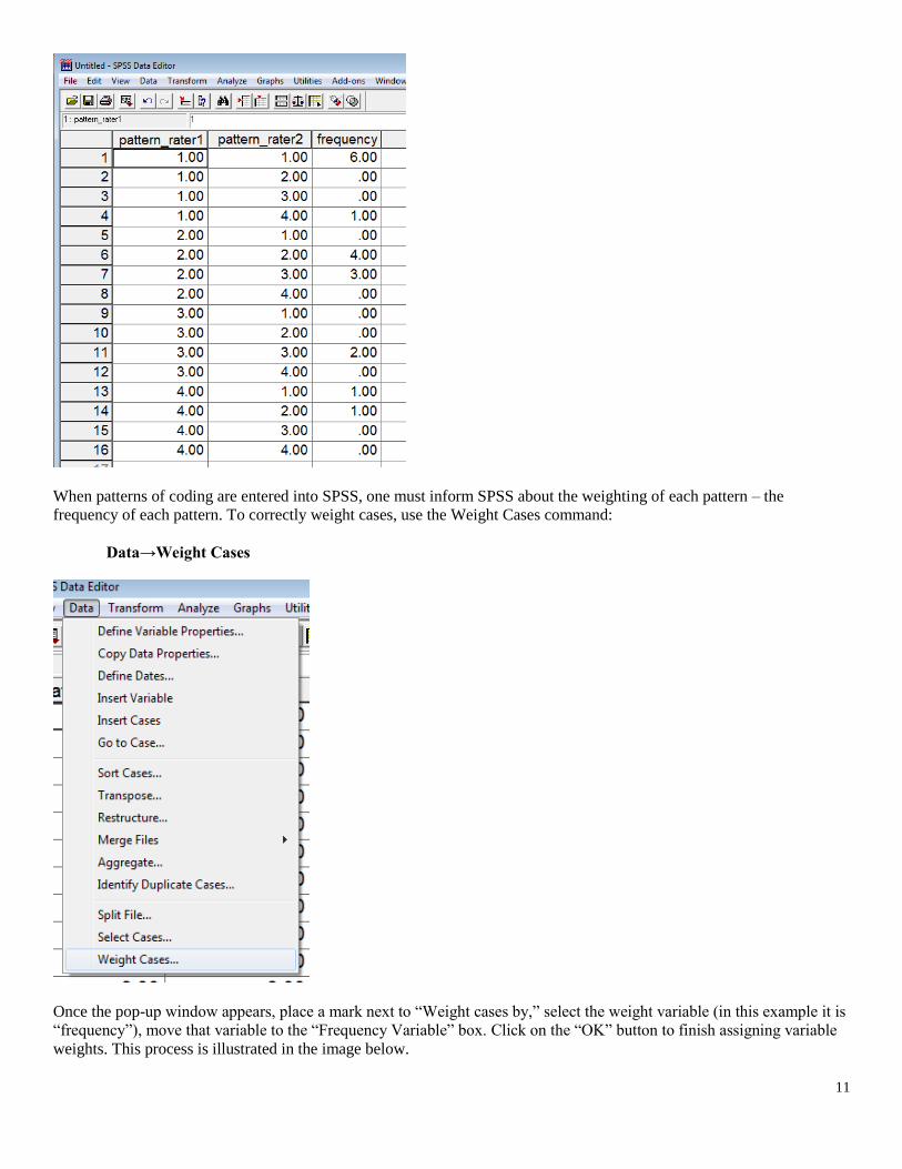
Example of data entry in SPSS appears below.

11

When patterns of coding are entered into SPSS, one must inform SPSS about the weighting of each pattern – the

frequency of each pattern. To correctly weight cases, use the Weight Cases command:

Data→Weight Cases

Once the pop-up window appears, place a mark next to “Weight cases by,” select the weight variable (in this example it is

“frequency”), move that variable to the “Frequency Variable” box. Click on the “OK” button to finish assigning variable

weights. This process is illustrated in the image below.

12

Once the weighting variable is identified, one may now run the crosstabs command as illustrated earlier:

Analyze → Descriptive Statistics → Crosstabs

With the Crosstabs pop-up menu, move the raters’ pattern coding to the Row and Column boxes. One rater’s pattern

should be identified as the row, the other as the column – which raters’ pattern is assigned to row or column is not

important. This is illustrated in the image below.

Next, select “Statistics” then place mark next to “Kappa”, click “Continue” then “OK” to run the analysis.

In this case kappa is, again, .526.

13

(d) SPSS Limitation with Cronbach’s kappa

UPDATE: Newer versions of SPSS (at least version 21, maybe earlier editions too) do not suffer from the problem

described below.

SPSS cannot calculate kappa if one rater does not use the same rating categories as another rater. Suppose two raters are

asked to rate an essay as either:

1 = pass

2 = pass with revisions

3 = fail

Essay Essay Rater 1 Essay Rater 2

1 1 1

2 1 1

3 1 1

4 2 2

5 2 2

6 2 2

7 2 2

8 2 2

9 2 2

10 2 2

11 3 2

12 3 2

13 3 2

14 3 2

Note that Rater 2 does not assign a rating of 3 to any essay.

When SPSS is used to assess kappa for these data if fails to provide an estimate since Rater 2 has not category 3 ratings.

UCLA Statistical Consulting Group provides a workaround explained here.

http://www.ats.ucla.edu/stat/spss/faq/kappa.htm

14

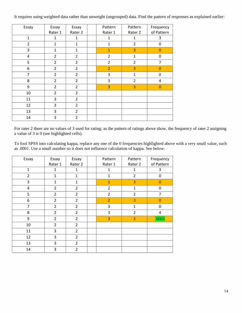
It requires using weighted data rather than unweight (ungrouped) data. Find the pattern of responses as explained earlier:

Essay Essay Rater 1

Essay Rater 2

Pattern Rater 1

Pattern Rater 2

Frequency of Pattern

1 1 1 1 1 3

2 1 1 1 2 0

3 1 1 1 3 0

4 2 2 2 1 0

5 2 2 2 2 7

6 2 2 2 3 0

7 2 2 3 1 0

8 2 2 3 2 4

9 2 2 3 3 0

10 2 2

11 3 2

12 3 2

13 3 2

14 3 2

For rater 2 there are no values of 3 used for rating; as the pattern of ratings above show, the frequency of rater 2 assigning

a value of 3 is 0 (see highlighted cells).

To fool SPSS into calculating kappa, replace any one of the 0 frequencies highlighted above with a very small value, such

as .0001. Use a small number so it does not influence calculation of kappa. See below:

Essay Essay Rater 1

Essay Rater 2

Pattern Rater 1

Pattern Rater 2

Frequency of Pattern

1 1 1 1 1 3

2 1 1 1 2 0

3 1 1 1 3 0

4 2 2 2 1 0

5 2 2 2 2 7

6 2 2 2 3 0

7 2 2 3 1 0

8 2 2 3 2 4

9 2 2 3 3 .0001

10 2 2

11 3 2

12 3 2

13 3 2

14 3 2

15

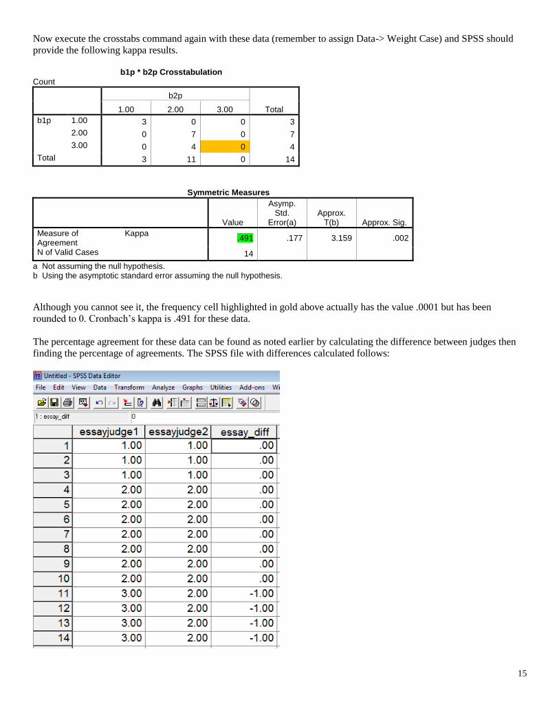
Now execute the crosstabs command again with these data (remember to assign Data-> Weight Case) and SPSS should

provide the following kappa results.

b1p * b2p Crosstabulation

Count

b2p

Total 1.00 2.00 3.00

b1p 1.00 3 0 0 3

2.00 0 7 0 7

3.00 0 4 0 4

Total 3 11 0 14

Symmetric Measures

Value

Asymp. Std.

Error(a) Approx.

T(b) Approx. Sig.

Measure of Agreement

Kappa .491 .177 3.159 .002

N of Valid Cases 14

a Not assuming the null hypothesis. b Using the asymptotic standard error assuming the null hypothesis.

Although you cannot see it, the frequency cell highlighted in gold above actually has the value .0001 but has been

rounded to 0. Cronbach’s kappa is .491 for these data.

The percentage agreement for these data can be found as noted earlier by calculating the difference between judges then

finding the percentage of agreements. The SPSS file with differences calculated follows:

16

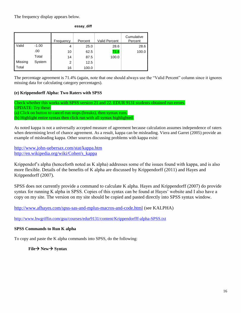
The frequency display appears below.

essay_diff

Frequency Percent Valid Percent Cumulative

Percent

Valid -1.00 4 25.0 28.6 28.6

.00 10 62.5 71.4 100.0

Total 14 87.5 100.0

Missing System 2 12.5

Total 16 100.0

The percentage agreement is 71.4% (again, note that one should always use the “Valid Percent” column since it ignores

missing data for calculating category percentages).

(e) Krippendorff Alpha: Two Raters with SPSS

Check whether this works with SPSS version 21 and 22. EDUR 9131 students obtained run errors.

UPDATE: Try these:

(a) Click on button to cancel run stops (breaks), then syntax runs.

(b) Highlight entire syntax then click run with all syntax highlighted.

As noted kappa is not a universally accepted measure of agreement because calculation assumes independence of raters

when determining level of chance agreement. As a result, kappa can be misleading. Viera and Garret (2005) provide an

example of misleading kappa. Other sources discussing problems with kappa exist:

http://www.john-uebersax.com/stat/kappa.htm

http://en.wikipedia.org/wiki/Cohen's_kappa

Krippendof’s alpha (henceforth noted as K alpha) addresses some of the issues found with kappa, and is also

more flexible. Details of the benefits of K alpha are discussed by Krippendorff (2011) and Hayes and

Krippendorff (2007).

SPSS does not currently provide a command to calculate K alpha. Hayes and Krippendorff (2007) do provide

syntax for running K alpha in SPSS. Copies of this syntax can be found at Hayes’ website and I also have a

copy on my site. The version on my site should be copied and pasted directly into SPSS syntax window.

http://www.afhayes.com/spss-sas-and-mplus-macros-and-code.html (see KALPHA)

http://www.bwgriffin.com/gsu/courses/edur9131/content/Krippendorfff-alpha-SPSS.txt

SPSS Commands to Run K alpha

To copy and paste the K alpha commands into SPSS, do the following:

File New Syntax

17

This opens a syntax window that should be similar to this window:

Now open the K alpha commands from this link

http://www.bwgriffin.com/gsu/courses/edur9131/content/Krippendorfff-alpha-SPSS.txt

Next, copy and paste everything find at that link into the SPSS syntax window. When you finish, it should look like this:

18

To make this syntax work four bits of the command line must be changed. The command line is the isolated line above

that reads:

KALPHA judges = judgelist/level = a/detail = b/boot = z.

judges = judgelist

These are the raters which form columns in SPSS

level = a

This is the scale of measurement of ratings with

1 = nominal

2 = ordinal

3 = interval

4 = ratio

Since we are dealing with ratings that are nominal, select 1 here.

detail = b

Specify 0 or 1 here; by default select 1 to see calculations.

boot = z

This options allows one to obtain bootstrapped standard errors for the K alpha estimate. For our purposes we

won’t request standard errors so place 0 for this option. If you wanted standard errors, the minimum replications

would be 1000.

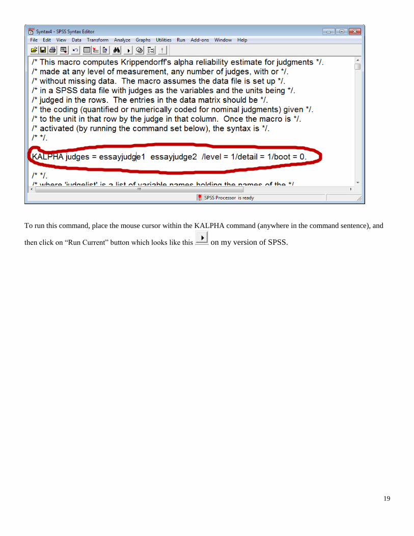
To obtain K alpha for the essay data below, make the following changes to the Kalpha command in the syntax window:

KALPHA judges = essayreader1 essayreader2 /level = 1/detail = 1/boot = 0.

So the SPSS syntax window now looks like this:

19

To run this command, place the mouse cursor within the KALPHA command (anywhere in the command sentence), and

then click on “Run Current” button which looks like this on my version of SPSS.

20

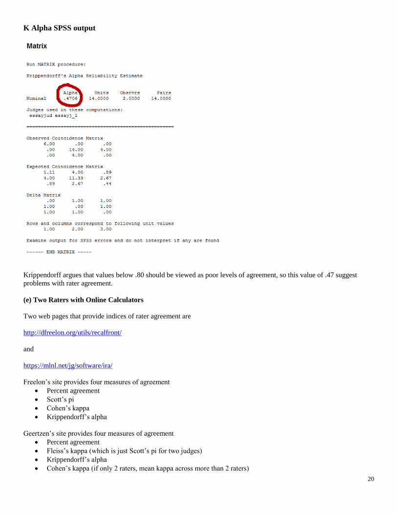
K Alpha SPSS output

Krippendorff argues that values below .80 should be viewed as poor levels of agreement, so this value of .47 suggest

problems with rater agreement.

(e) Two Raters with Online Calculators

Two web pages that provide indices of rater agreement are

http://dfreelon.org/utils/recalfront/

and

https://mlnl.net/jg/software/ira/

Freelon’s site provides four measures of agreement

Percent agreement

Scott’s pi

Cohen’s kappa

Krippendorff’s alpha

Geertzen’s site provides four measures of agreement

Percent agreement

Fleiss’s kappa (which is just Scott’s pi for two judges)

Krippendorff’s alpha

Cohen’s kappa (if only 2 raters, mean kappa across more than 2 raters)

21

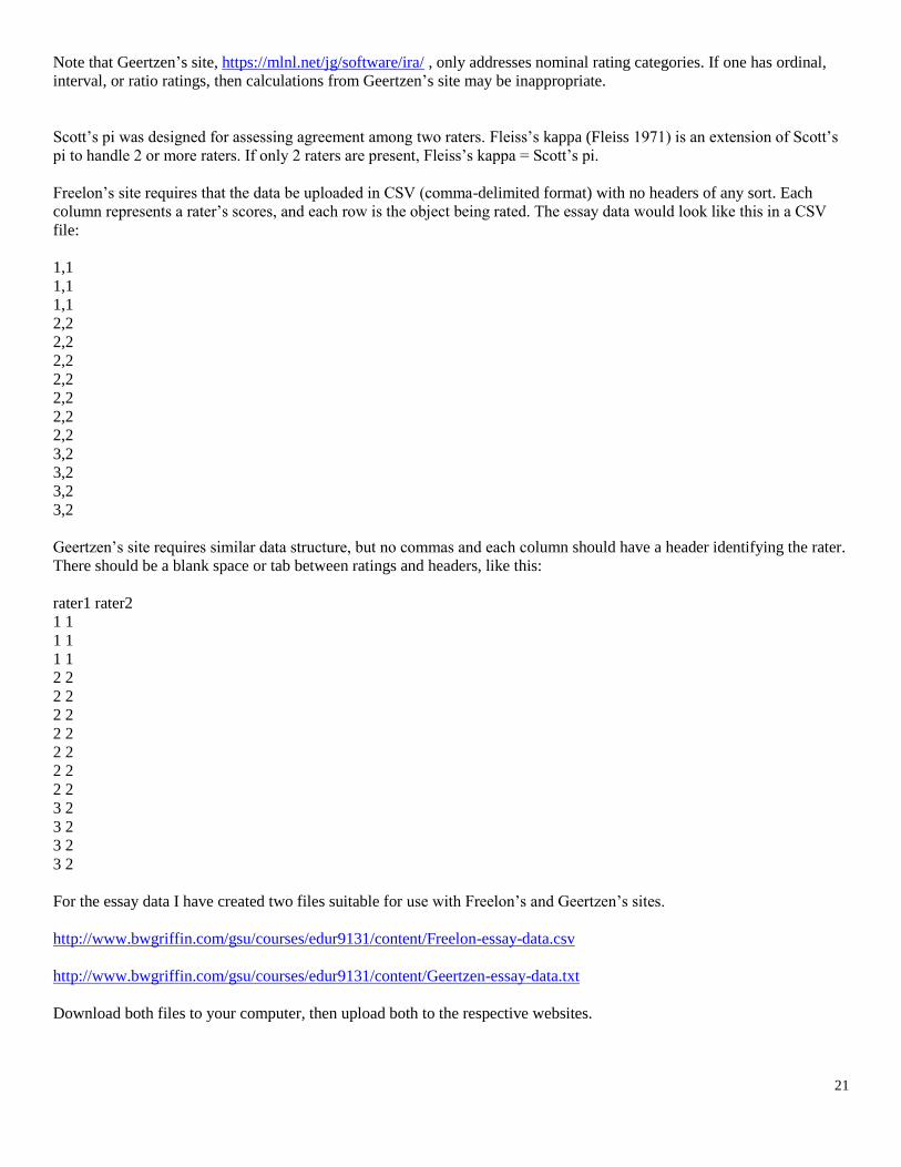
Note that Geertzen’s site, https://mlnl.net/jg/software/ira/ , only addresses nominal rating categories. If one has ordinal,

interval, or ratio ratings, then calculations from Geertzen’s site may be inappropriate.

Scott’s pi was designed for assessing agreement among two raters. Fleiss’s kappa (Fleiss 1971) is an extension of Scott’s

pi to handle 2 or more raters. If only 2 raters are present, Fleiss’s kappa = Scott’s pi.

Freelon’s site requires that the data be uploaded in CSV (comma-delimited format) with no headers of any sort. Each

column represents a rater’s scores, and each row is the object being rated. The essay data would look like this in a CSV

file:

1,1

1,1

1,1

2,2

2,2

2,2

2,2

2,2

2,2

2,2

3,2

3,2

3,2

3,2

Geertzen’s site requires similar data structure, but no commas and each column should have a header identifying the rater.

There should be a blank space or tab between ratings and headers, like this:

rater1 rater2

1 1

1 1

1 1

2 2

2 2

2 2

2 2

2 2

2 2

2 2

3 2

3 2

3 2

3 2

For the essay data I have created two files suitable for use with Freelon’s and Geertzen’s sites.

http://www.bwgriffin.com/gsu/courses/edur9131/content/Freelon-essay-data.csv

http://www.bwgriffin.com/gsu/courses/edur9131/content/Geertzen-essay-data.txt

Download both files to your computer, then upload both to the respective websites.

22

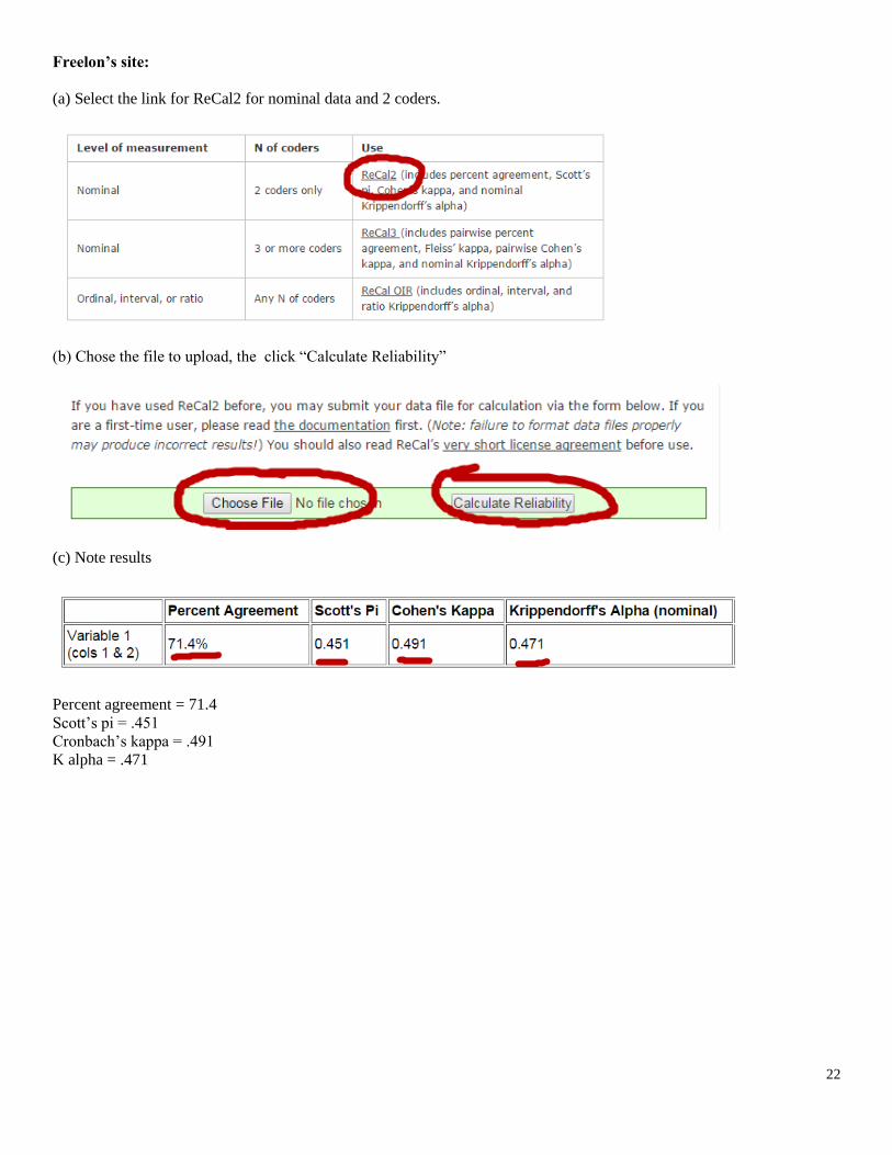
Freelon’s site:

(a) Select the link for ReCal2 for nominal data and 2 coders.

(b) Chose the file to upload, the click “Calculate Reliability”

(c) Note results

Percent agreement = 71.4

Scott’s pi = .451

Cronbach’s kappa = .491

K alpha = .471

23

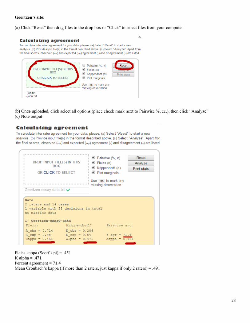
Geertzen’s site:

(a) Click “Reset” then drag files to the drop box or “Click” to select files from your computer

(b) Once uploaded, click select all options (place check mark next to Pairwise %, ec.), then click “Analyze”

(c) Note output

Fleiss kappa (Scott’s pi) = .451

K alpha = .471

Percent agreement = 71.4

Mean Cronbach’s kappa (if more than 2 raters, just kappa if only 2 raters) = .491

24

4. Two-coder Examples

(a) Usefulness of Noon Lectures

What would be various agreement indices for Viera and Garret (2005) data in table 1?

(b) Photographs of Faces

Example taken from Cohen, B. (2001). Explaining psychological statistics (2nd

ed). Wiley and Sons.

There are 32 photographs of faces expressing emotion. Two raters asked to categorize each according to these themes:

Anger, Fear, Disgust, and Contempt.

What would be the value of various fit indices these ratings?

Ratings of Photographed Faces

Rater 2

Anger Fear Disgust Contempt

Anger 6 0 1 2

Rater 1 Fear 0 4 2 0

Disgust 2 1 5 1

Contempt 1 1 2 4

Note: Numbers indicate counts, e.g., there are 6 cases in which raters 1 and 2 rated face as angry.

(c) Answers to be provided.

25

5. Nominal-scaled Codes: More than Two Raters

(a) Percent Agreement Among Multiple Raters

Recall the example of three raters provided in 2(c) above for hand calculation. The example is repeated below.

In situations with more than two raters, one method for calculating inter-rater agreement is to take the mean level of

agreement across all pairs of reviewers.

Participant Rater 1 Rater 2 Rater 3 Difference

Pair 1 and 2

Difference

Pair 1 and 3

Difference

Pair 2 and 3

1 1 1 1 0 0 0

1 2 2 2 0 0 0

1 3 3 3 0 0 0

2 2 3 3 -1 -1 0

2 1 4 1 -3 0 3

3 2 3 1 -1 1 2

3 2 2 4 0 -2 -2

4 1 1 1 0 0 0

4 4 1 1 3 3 0

5 1 1 1 0 0 0

6 2 2 2 0 0 0

7 3 3 3 0 0 0

8 1 1 1 0 0 0

9 1 1 2 0 -1 -1

9 4 2 2 2 2 0

10 2 2 2 0 0 0

11 1 1 1 0 0 0

11 2 3 4 -1 -2 -1

Total count of 0 in difference column = 12 11 13

Total Ratings = 18 18 18

Proportion Agreement = 12/18 = .6667 11/18 = .6111 13/18 = .7222

Percentage Agreement = 66.67 61.11 72.22

Overall Percentage Agreement = Mean agreement: 66.67%

(b) Mean Cronbach’s kappa

Some have suggested that one can calculate Cronbach’s kappa for each pair of raters, then take the mean value to form a

generalized measure of kappa (Hallgren, 2012; Warrens, 2010). The limitations with kappa noted above still apply here.

To illustrate, consider the data posted above for three raters.

For raters 1 and 2, kappa = .526

For raters 1 and 3, kappa = .435

For raters 2 and 3, kappa = .602

Mean kappa across all pairs = .521

26

(c) Fleiss kappa (pi)

As previously noted Fleiss extended Scott’s pi to multiple raters, but Fleiss named it kappa as an extension of Cronbach’s

kappa. The formula, however, follows more closely with Scott’s version for calculating expected agreement than

Cronbach’s version of expected agreement. This value can be interpreted like kappa. Illustrations will follow below.

(d) Krippendorff alpha

Krippendorff’s alpha can be extended to any number of raters, and can also handle missing data well, something the above

measures cannot handle well. Krippendorff’s alpha is interpreted as noted before, values below .80 should be viewed as

weak agreement.

The three rater data noted above are entered into SPSS as follows:

Using Haye’s K alpha syntax, the following command line is used:

KALPHA judges = r1 r2 r3 /level = 1/detail = 1/boot = 0.

The three judges are raters 1 through 3, denoted in SPSS as r1, r2, and r3. Level = 1 which means these are nominal scaled

ratings (categorical), and detail is 1 (show SPSS calculations).

SPSS Results

This is a similar version to the mean kappa calculated above. Results of K alpha suggest agreement is low among raters.

27

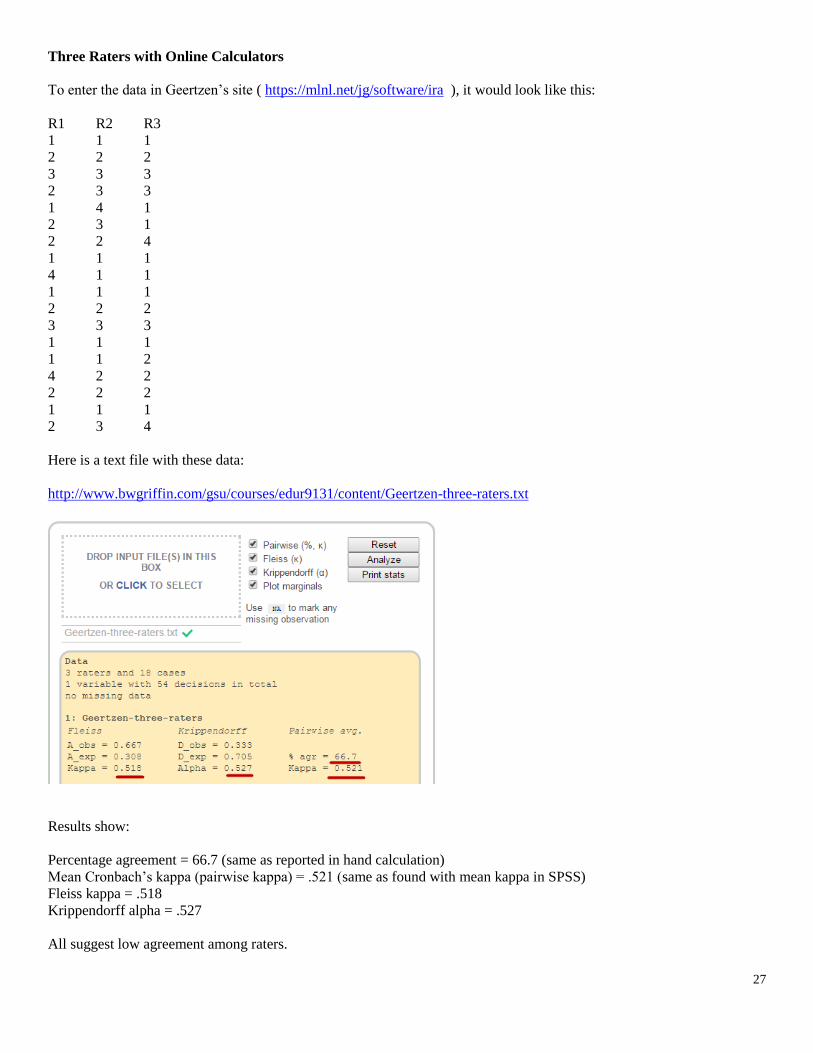
Three Raters with Online Calculators

To enter the data in Geertzen’s site ( https://mlnl.net/jg/software/ira ), it would look like this:

R1 R2 R3

1 1 1

2 2 2

3 3 3

2 3 3

1 4 1

2 3 1

2 2 4

1 1 1

4 1 1

1 1 1

2 2 2

3 3 3

1 1 1

1 1 2

4 2 2

2 2 2

1 1 1

2 3 4

Here is a text file with these data:

http://www.bwgriffin.com/gsu/courses/edur9131/content/Geertzen-three-raters.txt

Results show:

Percentage agreement = 66.7 (same as reported in hand calculation)

Mean Cronbach’s kappa (pairwise kappa) = .521 (same as found with mean kappa in SPSS)

Fleiss kappa = .518

Krippendorff alpha = .527

All suggest low agreement among raters.

28

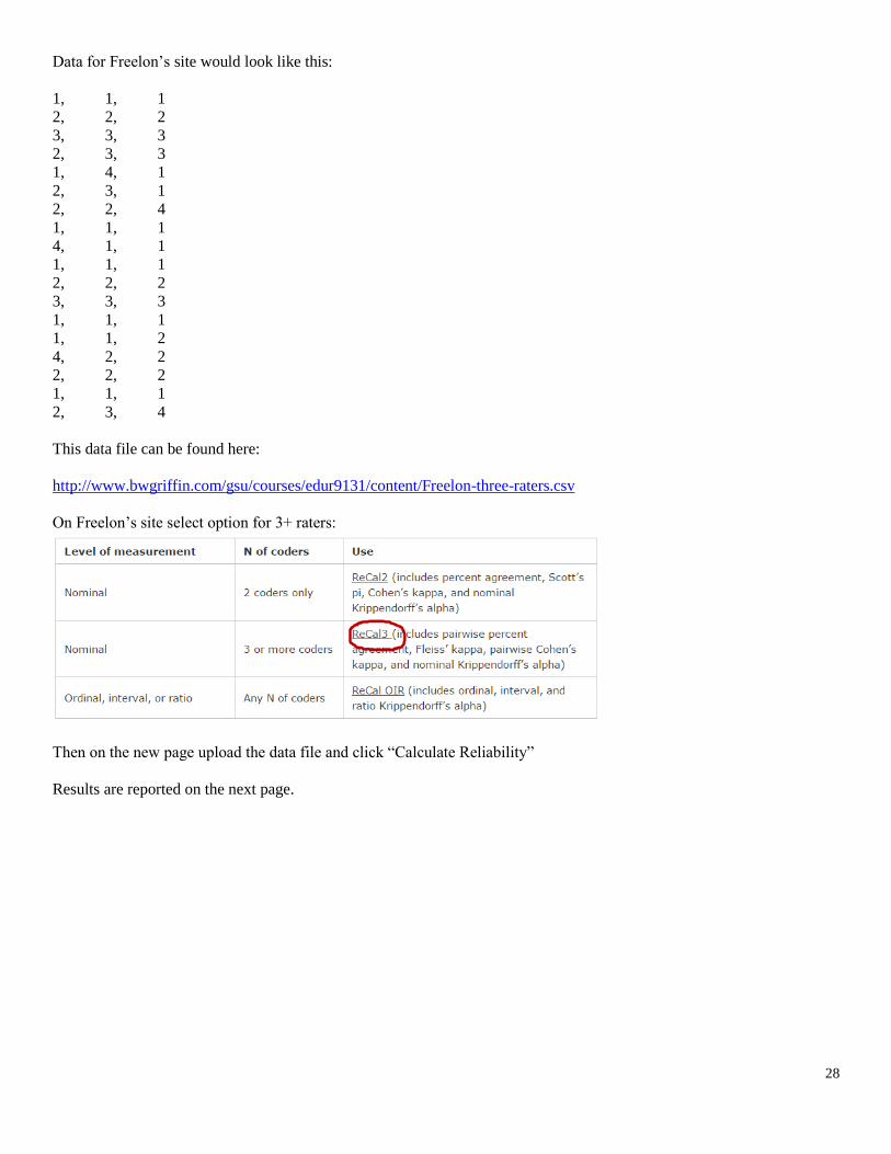
Data for Freelon’s site would look like this:

1, 1, 1

2, 2, 2

3, 3, 3

2, 3, 3

1, 4, 1

2, 3, 1

2, 2, 4

1, 1, 1

4, 1, 1

1, 1, 1

2, 2, 2

3, 3, 3

1, 1, 1

1, 1, 2

4, 2, 2

2, 2, 2

1, 1, 1

2, 3, 4

This data file can be found here:

http://www.bwgriffin.com/gsu/courses/edur9131/content/Freelon-three-raters.csv

On Freelon’s site select option for 3+ raters:

Then on the new page upload the data file and click “Calculate Reliability”

Results are reported on the next page.

29

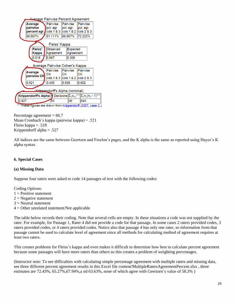
Percentage agreement = 66.7

Mean Cronbach’s kappa (pairwise kappa) = .521

Fleiss kappa = .518

Krippendorff alpha = .527

All indices are the same between Geertzen and Freelon’s pages, and the K alpha is the same as reported using Hayes’s K

alpha syntax.

6. Special Cases

(a) Missing Data

Suppose four raters were asked to code 14 passages of text with the following codes:

Coding Options:

1 = Positive statement

2 = Negative statement

3 = Neutral statement

4 = Other unrelated statement/Not applicable

The table below records their coding. Note that several cells are empty. In these situations a code was not supplied by the

rater. For example, for Passage 1, Rater 4 did not provide a code for that passage. In some cases 2 raters provided codes, 3

raters provided codes, or 4 raters provided codes. Notice also that passage 4 has only one rater, so information from that

passage cannot be used to calculate level of agreement since all methods for calculating method of agreement requires at

least two raters.

This creates problems for Fleiss’s kappa and even makes it difficult to determine how best to calculate percent agreement

because some passages will have more raters than others so this creates a problem of weighting percentages.

(Instructor note: To see difficulties with calculating simple percentage agreement with multiple raters and missing data,

see three different percent agreement results in this Excel file content/MultipleRatersAgreementPercent.xlsx , three

estimates are 72.43%, 65.27%,67.94%,a nd 63.63%, none of which agree with Geertzen’s value of 58.3% )

30

Krippendorff’s alpha, however, is designed to address such missing data and still provide a measure of rater agreement.

Passage Rater1 Rater2 Rater3 Rater4

1 1 2 1

2 1 2

3

1 1 1

4 1

5 1 1 2 1

6 2

2

7

1

1

8 2

3

9

2 2

10 3

3

11 3

2

12

1 1

13 4

4

14 4 4

Geertzen’s site can be used to find Krippendorff’s alpha. To identify missing data, Geertzen requires that missing data be

denoted with NA (capital NA, “na” won’t work). Below is a revised table to meet Geertzen’s specifications.

Passage Rater1 Rater2 Rater3 Rater4

1 1 2 1 NA

2 1 2 NA NA

3 NA 1 1 1

4 1 NA NA NA

5 1 1 2 1

6 2 NA 2 NA

7 NA 1 NA 1

8 2 NA 3 NA

9 NA 2 2 NA

10 3 NA NA 3

11 3 NA NA 2

12 NA NA 1 1

13 4 NA NA 4

14 4 4 NA NA

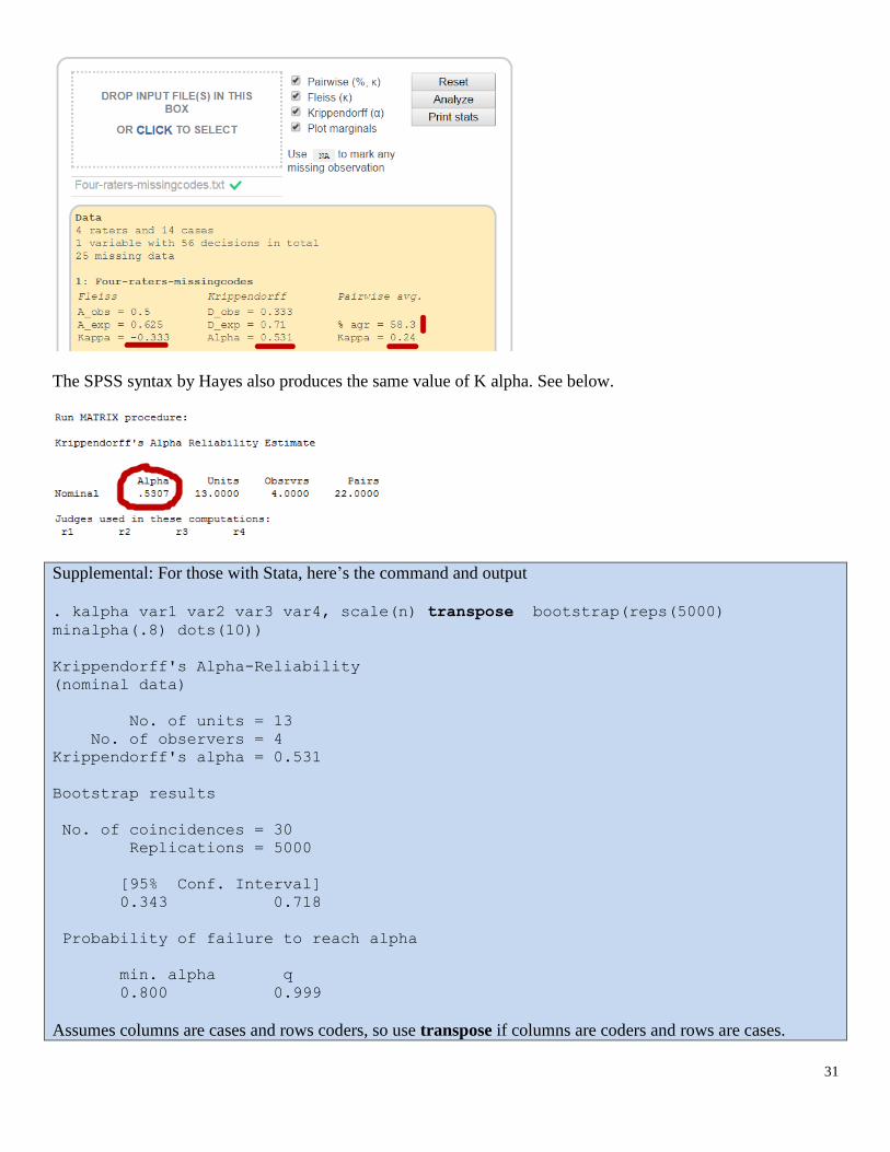
Results of Geertzen’s calculations are presented below.

31

The SPSS syntax by Hayes also produces the same value of K alpha. See below.

Supplemental: For those with Stata, here’s the command and output

. kalpha var1 var2 var3 var4, scale(n) transpose bootstrap(reps(5000)

minalpha(.8) dots(10))

Krippendorff's Alpha-Reliability

(nominal data)

No. of units = 13

No. of observers = 4

Krippendorff's alpha = 0.531

Bootstrap results

No. of coincidences = 30

Replications = 5000

[95% Conf. Interval]

0.343 0.718

Probability of failure to reach alpha

min. alpha q

0.800 0.999

Assumes columns are cases and rows coders, so use transpose if columns are coders and rows are cases.

32

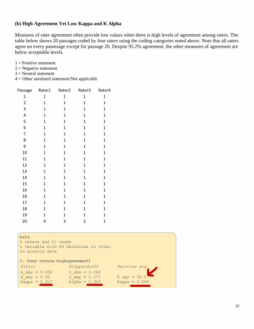
(b) High Agreement Yet Low Kappa and K Alpha

Measures of rater agreement often provide low values when there is high levels of agreement among raters. The

table below shows 20 passages coded by four raters using the coding categories noted above. Note that all raters

agree on every passesage except for passage 20. Despite 95.2% agreement, the other measures of agreement are

below acceptable levels.

1 = Positive statement

2 = Negative statement

3 = Neutral statement

4 = Other unrelated statement/Not applicable

Passage Rater1 Rater2 Rater3 Rater4

1 1 1 1 1

2 1 1 1 1

3 1 1 1 1

4 1 1 1 1

5 1 1 1 1

6 1 1 1 1

7 1 1 1 1

8 1 1 1 1

9 1 1 1 1

10 1 1 1 1

11 1 1 1 1

12 1 1 1 1

13 1 1 1 1

14 1 1 1 1

15 1 1 1 1

16 1 1 1 1

16 1 1 1 1

17 1 1 1 1

18 1 1 1 1

19 1 1 1 1

20 4 3 2 1

33

The problem with these data is lack of variability in codes. When most raters assign one code predominately,

then measures of agreement can be misleadingly low, as demonstated in this example. This is one reason I

recommend always reporting percent agreement.

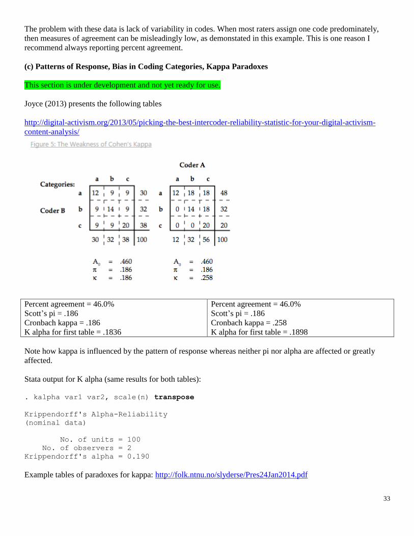
(c) Patterns of Response, Bias in Coding Categories, Kappa Paradoxes

This section is under development and not yet ready for use.

Joyce (2013) presents the following tables

http://digital-activism.org/2013/05/picking-the-best-intercoder-reliability-statistic-for-your-digital-activism-

content-analysis/

Percent agreement = 46.0%

Scott’s pi = .186

Cronbach kappa = .186

K alpha for first table = .1836

Percent agreement = 46.0%

Scott’s pi = .186

Cronbach kappa = .258

K alpha for first table = .1898

Note how kappa is influenced by the pattern of response whereas neither pi nor alpha are affected or greatly

affected.

Stata output for K alpha (same results for both tables):

. kalpha var1 var2, scale(n) transpose

Krippendorff's Alpha-Reliability

(nominal data)

No. of units = 100

No. of observers = 2

Krippendorff's alpha = 0.190

Example tables of paradoxes for kappa: http://folk.ntnu.no/slyderse/Pres24Jan2014.pdf

34

References

Fleiss (1971) Measuring Nominal Scale Agreement Among Many Raters. Psychological Bulletin, 76, 378-382.

http://www.bwgriffin.com/gsu/courses/edur9131/content/Fleiss_kappa_1971.pdf

Hayes, A. F. & Krippendorfff, K. (2007). Answering the call for a standard reliability measure for

coding data. Communication Methods and Measures, 1, 77-89.

http://www.bwgriffin.com/gsu/courses/edur9131/content/coding_reliability_2007.pdf

Hallgren, K.A. (2012). Computing Inter-rater Reliability for Observational Data: An Overview and Tutorial. Tutor Quant.

Psychol., 23-34.

http://www.ncbi.nlm.nih.gov/pmc/articles/PMC3402032/pdf/nihms372951.pdf

Joyce (2013) Blog Entry: Picking the Best Intercoder Reliability Statistic for Your Digital Activism Content Analysis

http://digital-activism.org/2013/05/picking-the-best-intercoder-reliability-statistic-for-your-digital-activism-

content-analysis

Krippendorfff, K. (2011). Agreement and Information in the Reliability of Coding. Communication Methods and

Measures, 5 (2), 93-112. http://dx.doi.org/10.1080/19312458.2011.568376

http://repository.upenn.edu/cgi/viewcontent.cgi?article=1286&context=asc_papers

Scott, W. (1955). "Reliability of content analysis: The case of nominal scale coding." Public Opinion Quarterly, 19(3),

321-325.

http://en.wikipedia.org/wiki/Scott's_Pi

Warrens, M. J. (2010). Inequalities between multi-rater kappas. Adv Data Anal Classif, 4, 271-286.

https://openaccess.leidenuniv.nl/bitstream/handle/1887/16237/Warrens_2010_ADAC_4_271_286.pdf?sequence=

2

Viera, A.J. & Garrett, J.M. (2005). Understanding interobserver agreement: The Kappa statistic. Family Medicine. 360-

363.

http://www.bwgriffin.com/gsu/courses/edur9131/content/Kappa_statisitc_paper.pdf