Interaction of Turing and Hopf Modes in the Superdiffusive...

Math. Model. Nat. Phenom.Vol. 6, No. 1, 2011, pp. 87-118

DOI: 10.1051/mmnp/20116105

Interaction of Turing and Hopf Modesin the Superdiffusive Brusselator Model

Near a Codimension Two Bifurcation Point

J.C. Tzou, A. Bayliss, B.J. Matkowsky ∗ and V.A. Volpert

Department of Engineering Sciences and Applied MathematicsNorthwestern University, Evanston IL 60208-3125 USA

This paper is dedicated to the memory of our colleague and friend Alexander (Sasha) Golovin

Abstract. Spatiotemporal patterns near a codimension-2 Turing-Hopf point of the one-dimensionalsuperdiffusive Brusselator model are analyzed. The superdiffusive Brusselator model differs fromits regular counterpart in that the Laplacian operator of the regular model is replaced by ∂α/∂ |ξ|α,1 < α < 2, an integro-differential operator that reflects the nonlocal behavior of superdiffusion.The order of the operator, α, is a measure of the rate of superdiffusion, which, in general, canbe different for each of the two components. A weakly nonlinear analysis is used to derive twocoupled amplitude equations describing the slow time evolution of the Turing and Hopf modes.We seek special solutions of the amplitude equations, namely a pure Turing solution, a pure Hopfsolution, and a mixed mode solution, and analyze their stability to long-wave perturbations. Wefind that the stability criteria of all three solutions depend greatly on the rates of superdiffusion ofthe two components. In addition, the stability properties of the solutions to the anomalous diffusionmodel are different from those of the regular diffusion model. Numerical computations in a largespatial domain, using Fourier spectral methods in space and second order Runge-Kutta in timeare used to confirm the analysis and also to find solutions not predicted by the weakly nonlinearanalysis, in the fully nonlinear regime. Specifically, we find a large number of steady state patternsconsisting of a localized region or regions of stationary stripes in a background of time periodiccellular motion, as well as patterns with a localized region or regions of time periodic cells in abackground of stationary stripes. Each such pattern lies on a branch of such solutions, is stable and

∗Corresponding author. E-mail: [email protected]

87

J.C. Tzou et al. Interaction of Turing and Hopf modes near C2THP

corresponds to a different initial condition. The patterns correspond to the phenomenon of pinningof the front between the stripes and the time periodic cellular motion. While in some cases it is dif-ficult to isolate the effect of the diffusion exponents, we find characteristics in the spatiotemporalpatterns for anomalous diffusion that we have not found for regular (Fickian) diffusion.

Key words: Brusselator model, superdiffusion, Turing pattern, Hopf bifurcation, codimension-2bifurcation, weakly nonlinear analysis, amplitude equations, spatiotemporal patternsAMS subject classification: 35B36, 35K57, 35Q99, 37G99

1 IntroductionStudies of anomalous diffusion have recently been appearing in the literature as more processeshave been observed to exhibit behavior that cannot be described by regular (Fickian) diffusion.These processes can often be described by models with subdiffusion or superdiffusion, where,under a random walk description, the mean square displacement of a particle scales as 〈x2(t)〉 ∼ tγ ,with 0 < γ < 1 for subdiffusion, and 1 < γ < 2 for superdiffusion, rather than linearly intime. Subdiffusion has been observed in many applications, including charge carrier transportin amorphous semiconductors, and nuclear magnetic resonance diffusometry in percolative andporous systems, while superdiffusion has been observed in e.g., transport in heterogeneous rocks,quantum optics, and single molecule spectroscopy [10]. We consider an especially interesting caseof superdiffusion, Levy flights, which is characterized by a jump length distribution having infinitemoments. On the macroscopic scale, Levy flights are described by a diffusion equation wherethe second order spatial derivative is replaced by a fractional derivative ∂α/∂ |ξ|α, 1 < α < 2,defined as a non-local integro-differential operator [10]. Previous works on reaction-superdiffusionequations have derived and studied amplitude equations near a Hopf [11] or Turing [8] bifurcationpoint. In this paper, we investigate the effects of superdiffusion on the interactions between Hopfand Turing instabilities of the Brusselator model by deriving amplitude equations and studyinginstabilities of their solutions to long-wave perturbations, thus leading to the identification of theparameter values at which new solutions may bifurcate. Similar studies near a codimension-twoTuring-Hopf point (C2THP) of the regular Brusselator model have been done in [7], [15]. Wealso discuss the results of numerical computations in both the weakly and fully nonlinear regimes.In this paper, we consider both the regular and superdiffusive one-dimensional Brusselator modeland identify characteristics of spatiotemporal patterns obtained near the C2THP that are unique toeach. In the anomalous case, we consider cases of equal diffusion exponents, unequal but closediffusion exponents, and where one diffusion is regular while the other is anomalous.

88


2 The model, the basic solution, and its linear stabilityWe consider the Brusselator model, long a paradigm for nonlinear analysis, given by

∂f

∂τ= Df

∂αf

∂ |ξ|α + E − (B + 1)f + f 2g (2.1)

∂g

∂τ= Dg

∂βg

∂ |ξ|β + Bf − f 2g, τ > 0, ξ ∈ R. (2.2)

The diffusion coefficients Df , Dg, the activator input rate E, and the control parameter B, arepositive quantities. The action of the operator ∂γ/∂ |ξ|γ in Fourier space is

F [∂γu(ξ)/∂ |ξ|γ](k) = −|k|γF [u(ξ)](k), 1 < γ < 2. (2.3)

The equilibrium (basic) state of this system is (f, g) = (E, B/E) for all values of the parameters.Rescaling (2.1) and (2.2) using f = E + u∗u, g = B/E + v∗v, τ = t, and ξ = `∗x, where

u∗ = (Dg/Dβ/αf )1/2, v∗ = 1/u∗, and `∗ = D

1/αf , the Brusselator system becomes

∂u

∂t=

∂αu

∂ |x|α + (B − 1)u + Q2v +B

Qu2 + 2Quv + u2v (2.4)

η2∂v

∂t=

∂βv

∂ |x|β −Bu−Q2v − B

Qu2 − 2Quv − u2v, (2.5)

where η =√

Dβ/αf /Dg > 0, Q = Eη > 0, and x and t represent the rescaled spatial and temporal

variables, respectively. The equilibrium state is now at u = v = 0.To determine the stability of the critical point, we consider the normal mode solution, obtaining

the dispersion relation between the growth rate σ and the wave number k > 0, η2σ2+M1σ+M2 =0, where M1 = Q2 + kβ − η2(B − 1− kα), and M2 = BQ2 + (kβ + Q2)(1 + kα −B).

Hopf bifurcation occurs if M1 = 0 and M2 > 0, which yields two pure imaginary eigenvalues.M1 = 0 corresponds to B = kβ/η2 + kα + 1 + Q2/η2, which has a minimum, B

(H)cr = 1 + Q2/η2

at k = 0. The basic state is stable (unstable) for B < B(H)cr (B > B

(H)cr ). In the unstable case,

a spatially homogeneous oscillatory mode emerges. For k = 0 and B = B(H)cr , the eigenvalue

σ = iQ/η ≡ iω, where ω is the frequency of the oscillatory mode, while c† = (1, Qη2/(Q + iη))

and c = (1, (iη −Q)/(Qη2))> are the left and right eigenvectors, respectively.

Turing instability occurs when M2 = 0 and M1 > 0, which yields B = (Q2 + kβ)(1+ kα)/kβ .It has a single minimum (kcr, B

(T )cr ), given parametrically by

B(T )cr =

(1 + z)2

1 + (1− s)z, Q2 =

sz1+1/s

1 + (1− s)z, kcr = z1/α,

where s = α/β. Since Q is real, we find that 0 < z < ∞ if 1/2 < s ≤ 1, and 0 < z < 1/(s− 1) if1 < s < 2. The corresponding left and right eigenvectors of the zero eigenvalue are, respectively,

89


a† = (1, szη2c/(1 + z)) and a =

(z1/s,−1− z

)>. For the Turing instability, a time-independentspatially periodic pattern may emerge with spatial wave number k = kcr.

Turing and Hopf instability thresholds coincide at the C2THP where B = B(T )cr = B

(H)cr ≡ Bcr,

which occurs when η = ηc ≡√

sz1/s/(z + s + 1). Thus, as the control parameter B is increasedbeyond Bcr, a Turing mode and a Hopf mode simultaneously bifurcate from the basic state, givingrise to terms of the form Aaeikcrx and Cceiωt in (u, v)>. We note that Bcr, Q, ηc, and the activatorinput rate, E = Q/ηc, are increasing functions of z for all allowed values of z.

3 Weakly nonlinear analysisWe analyze the system near the C2THP, i.e., let η = ηc + ε2η2 (0 < ε ¿ 1). If η2 > 0 (< 0), theHopf (Turing) mode appears first as the parameter B is increased. We interpret this as changingthe parameter E, keeping Q constant. Thus, changing η2 will only affect the Hopf stability curve,not the Turing curve. Also, let B = Bcr + ε2µ, where µ > 0 is a real O(1) quantity. This leads tothe presence of two time scales. The original time scale, t, appears with oscillation frequency ω,while the slow time scale, T = ε2t, accounts for the slow-time evolution of the Turing and Hopfmodes. The three relevant spatial scales are x, X1 = εx, and X2/α = ε2/αx, where the scaling forX2/α is chosen under the condition that α < β. If α > β, the third spatial scale would instead beX2/β . While we consider both cases in Section 4, the explicit expressions are for α < β.

With the relevant scales established, we allow for the possibility of both A and C to be functionsof the slow time scale as well as the two long spatial scales. Then, since the Turing mode may bea function of all three spatial scales and the Hopf mode a function of the two long spatial scales,we require analogues of the chain rule to obtain expressions for how the operator ∂γ/∂ |x|γ actson u and v. While nothing in the linear stability analysis of Section 2 prevents the Hopf modefrom being a function of the two long spatial scales, solvability conditions discussed below inthe weakly nonlinear analysis limit the Hopf mode dependence to X2/α only. Then, since theexpression obtained by applying dγ/d|x|γ to a function of the form F (x, X1, X2/α) does not reduceto the expression obtained by applying the operator to a function of the form G(X2/α) simply byletting ∂/∂x = ∂/∂X1 = 0, we decompose the solutions u and v into sums of functions ofthe form F (x,X1, X2/α, t, T ) and G(X2/α, t, T ). Since F accounts for all x-dependent terms,whether or not they depend on X1 and/or X2/α, while G accounts for all x-independent terms, thisdecomposition captures all possible terms that can arise in u and v. We utilize the product rule [12]for 1 < γ < 2,

dγ(fg)

d|x|γ =∞∑

j=0

(γj

)dγ−jf

d|x|γ−j

djg

dxj,

to compute

90


dγF (x,X1, X2/α)

d|x|γ =

(∂γ

∂|x|γ + γ∂γ−1

∂|x|γ−1

(ε

∂

∂X1

+ ε2/α ∂

∂X2/α

)+

+ ε2γ(γ − 1)

2

∂γ−2

∂|x|γ−2

∂2

∂X21

+ . . .

)F (x,X1, X2/α), (3.1)

where we have discarded terms smaller than O(ε2). The computation of dγG(X2/α)/d|x|γ requiresa simpler version of the chain rule, which gives dγG/d|x|γ = ε2γ/αdγG/d|X2/α|γ , where γ is eitherα or β.

Due to the fractional powers of ε in (3.1), we include fractional powers in the expansions of uand v:

(uv

)∼ ε

(u1

v1

)+ε2/α

(u2/α

v2/α

)+ε2

(u2

v2

)+ε1+2/α

(u1+2/α

v1+2/α

)+ε3

(u3

v3

)+ . . . . (3.2)

We decompose ui and vi as

(ui

vi

)=

(u

(A)i (x,X1, X2/α, t, T )

v(A)i (x, X1, X2/α, t, T )

)+

(u

(C)i (X2/α, t, T )

v(C)i (X2/α, t, T )

), (3.3)

where we associate the letter A with the Turing mode (though u(A)i and v

(A)i also account for

products of pure Turing and pure Hopf terms), and the letter C with the Hopf mode. If α > 4/3,we must also include an O(ε4/α) term in the expansion. Recalling the decomposition in (3.3), wesubstitute (3.2) into (2.4) and (2.5), and find that u1 and v1 satisfy

(∂

∂t− D0D −M0

) (u

(A)1

v(A)1

)+

(∂

∂t−M0

) (u

(C)1

v(C)1

)= 0, (3.4)

where

D0 =

(1 0

0 1η2

c

), D ≡

∂α

∂|x|α 0

0 ∂β

∂|x|β

, M0 =

(Bcr − 1 Q2

−Bcr

η2c

−Q2

η2c

).

Thus(

u1

v1

)= A(X1, X2/αT )aeikcrx + C(X2/α, T )ceiωt + c.c.,

where c.c. denotes complex conjugate. We have allowed only A to depend on both long scales. Ifwe had assumed that C also depended on both long scales, O(εα) and O(εβ) terms would need tobe included in (3.2). In this case, solvability conditions at O(ε1+α) and O(ε1+β) would require thatC be independent of X1. These are the solvability conditions mentioned above that dictate that

91


the Hopf mode can only be a function of X2/α. To see this, we apply the fractional operator to afunction of the form H(X1, X2/α):

dγH(X1, X2/α)

d|x|γ =

(εγ ∂γ

∂|X1|γ + εγ−1+2/αγ∂γ−1

∂|X1|γ−1

∂

∂X2/α

+

+ εγ−2+4/α γ(γ − 1)

2

∂γ−2

∂|X1|γ−2

∂2

∂X22/α

+ . . .

)H(X1, X2/α). (3.5)

The presence of an O(εγ) term in (3.5) would require that we include terms of O(εα), O(εβ),O(ε1+α), and O(ε1+β) in the expansion of u in (3.2), among terms of other orders. The right handside of the O(ε1+α) equation would then contain a secular-producing term

(10

)∂αC

∂|X1|α eiωt,

which is not orthogonal to c†, and thus the solvability condition is not met. A similar violation ofthe solvability condition is also seen at O(ε1+β), and also in the case of α = β. To avoid this, wedo not allow C to depend on X1.

The O(ε2/α) equation is the same as the O(ε) equation, with u2/α and v2/α satisfying the samehomogeneous equation as u1 and v1. Thus we may take u2/α = v2/α = 0 without loss of generality(the same applies for u4/α and v4/α).

While the left hand side of the O(ε2) equation is the same as that in (3.4), its right hand sidecontains secular-producing terms proportional to eikcrx. However, the solvability condition is sat-isfied (the secular-producing terms are orthogonal to a†), which leads to the solution

(u2

v2

)= A2p2se

i2kcrx+C2p2tei2ωt+ACpLeiφL+AC∗pReiφR+|A|2p0s+|C|2p0t+pse

ikcrx+c.c.,

where φL = kcrx + ωt and φR = kcrx− ωt.The O(ε1+2/α) equation, like the O(ε2) equation, contains secular-producing terms orthogonal

to a†. However, while u1+2/α and v1+2/α are non-zero, they do not enter the O(ε3) equation. Uponsolving for the vectors p2s, p2t, etc., and applying the solvability condition at O(ε3), we obtain,upon rescaling, the amplitude equations

∂A

∂T= A +

∂2A

∂X21

+ ζA|A|2 + ψ2A|C|2, (3.6)

∂C

∂T= ρC + (α1 + iα2)

∂αC

∂|X2/α|α + (−|β1|+ iβ2) C|C|2 + (δ1 + iδ2) C|A|2, (3.7)

where ζ = ±1, depending on the values of α, β, and z, while ψ2, α1, α2, β1, β2, δ1, and δ2, are realfunctions of α, β, and z. The coefficient ρ, while also real, is a function of α, β, and z, as well asµ and η2. Finally, it can be shown that α1 > 0.

92


We restrict z to the interval I such that ζ = −1, i.e., there exists nonlinear saturation of theTuring mode. We also note that (3.6) and (3.7) were derived under the necessary condition that Cbe independent of X1. Since (3.7) contains terms involving both A and C, |A| must be spatiallyhomogeneous. Thus, (3.6) and (3.7) describe only amplitudes A whose dependence on X1 takesthe form eih(X1) for a real function h. Since A can depend on both X1 and X2/α, there are norestrictions on the way in which C can depend on X2/α.

Lastly, the techniques used here resemble those used for the regular diffusion Brusselatormodel. There are, however, important differences, one being that two long spatial scales arepresent instead of the single long scale X1 in the regular model. Secondly, the expansions of uand v include fractional orders of ε, whereas only integer powers were required in the regularmodel. Thirdly, the rules of differentiation require that the solution be decomposed into separatefunctions that depend differently on the relevant variables. The resulting form of the amplitudeequations are also different in that the equation for C is now an integro-differential equation. Ashorter version of this section is presented in [14].

4 Solutions of the amplitude equations and their long-wave in-stabilities

In this section, we seek special solutions of (3.6) and (3.7), namely a pure Turing solution, apure Hopf solution, and a mixed mode solution. We then study the instabilities of these solutionsto long-wave perturbations. We first consider the pure Turing solution, given by C = 0 andA = AeiKAX1 with A = (1 − K2

A)1/2. To study its stability, we linearize around it using A =(A + a(X1, T ))eiKAX1 , and C = c(X2/α, T ). The resulting linearized equations decouple, so weanalyze each separately. A long-wave perturbation a(X1, T ) yields the familiar Eckhaus stabilitycriterion

|KA| < 1√3. (4.1)

If (4.1) is not satisfied, the perturbation grows, changing the spatial frequency of the solution. Along-wave perturbation c(X2/α, T ) with wave number k ¿ 1 results in the dispersion relationσ = ρ − α1|k|α + A2δ1 ± i| − α2|k|α + A2δ2|, whose real part must be negative for long-wavestability. If the real part is positive, the perturbation grows, changing the spatial structure of thesolution and also introducing a time-oscillatory component. The long-wave stability criterion isρ + A2δ1 < 0. If δ1 < 0, long-wave perturbations of the Hopf amplitude decay for all ρ < 0, oreven if ρ > 0 as long as ρ remains sufficiently small. If δ1 > 0, long-wave perturbations of theHopf amplitude can grow even for ρ < 0, as long as ρ is sufficiently close to 0.

For the regular diffusion model, δ1 > 0 for z . 0.26, or equivalently, ηc . 0.34, meaningthat the inhibitor (g) diffuses significantly faster than the activator (f ). In the anomalous model,we obtain an analogous result for α and β, since these two parameters have a greater impact onthe rate of diffusion than do the diffusion coefficients. In contrast to the regular model, δ1 can

93


be positive even if α < β, that is, if the inhibitor diffuses more slowly than the activator. Forα . 1.65, δ1 < 0 for all z ∈ I , meaning that sufficiently fast diffusion of the activator makes itimpossible for long-wave perturbations of the Hopf mode to grow if ρ < 0. This behavior is notseen in the regular model.

Next, we consider the pure Hopf solution, given by A = 0 and C = CeiKCX2/α+iΩT withC = ((ρ − α1|KC |α)/|β1|)1/2 and Ω = −α2|KC |α + β2C

2. We note that, since the quantityρ − α1|KC |α must be positive, ρ must be positive for the pure Hopf solution to exist. Long-waveperturbations of the form eσT+ikX2/α yield two growth rates, one of which is negative, the other ofwhich has the expansion for small k, σ = a1k + a2k

2 + O(k3), where

a1 = −iα (α1β2 + α2|β1|) |KC |α−1

|β1|and

a2 =α(α− 1) (α2β2 − α1|β1|)

2|β1| +α2α2

1(β21 + β2

2)|KC |α2|β1|3C2

.

Requiring a2 < 0 for stability leads to the generalized Eckhaus criterion,

|KC |α <ρ

Rα1

(4.2)

where

R = 1 +αα1 (β2

1 + β22)

(α− 1)|β1|(α1|β1| − α2β2).

Thus, if (4.2) is not satisfied, both the spatial and temporal structures of the solution are alteredas a long-wave perturbation grows with amplitude oscillating at a frequency different from Ω. Asin the regular diffusion case, the magnitude of R is greater than unity for all z ∈ I . However, ifα < β, unlike the regular diffusion case, R is positive only for z sufficiently small. Beyond thisinterval, R becomes negative so that (4.2) is never satisfied, in which case the pure Hopf solutionmust be long-wave unstable. Restricting z to sufficiently small values for which R is positiveimplies that Bcr, Q, ηc, and E, must all be sufficiently small. For example, ηc must be less than∼ 0.62, and thus, while the rate of diffusion is dominated by the diffusion exponents α and β, ηc

still impacts whether or not the Hopf mode can be long-wave stable. Note, however, that ηc is nota strict comparison between the diffusion coefficients Df and Dg, as these parameters do not evenhave the same units. The qualitative behavior of R in the α > β case is the same as for regulardiffusion, where R > 1 for all z ∈ I , suggesting that faster diffusion of the activator versus theinhibitor may contribute to instability of the pure Hopf solution.

Finally we consider the mixed mode solution, given by A = AeiKAX1 and C = CeiKCX2/α+iΩT

with

A =

(ψ2 (ρ− α1|KC |α) + |β1| (1−K2

A)

∆

)1/2

, C =

(ρ− α1|KC |α + δ1 (1−K2

A)

∆

)1/2

,

94


where ∆ = |β1| − ψ2δ1, and Ω = −α2|KC |α + β2C2 + δ2A

2. Of course, we must restrict KA andKC so that A and C are real. Linearizing (3.6) and (3.7) around this mixed mode solution withsmall perturbations a(X2/α, T ) and c(X2/α, T ) results in the coupled equations

∂a

∂T= (1−K2

A)a− A2(a∗ + 2a) + ψ2

[AC (c∗ + c) + aC2

], (4.3)

and

∂c

∂T= −iΩc + ρc + (α1 + iα2)

(−|KC |αc + iα|KC |α−1 ∂c

∂X2/α

+α(α− 1)

2|KC |α−2 ∂2c

∂X22/α

)

+ (−|β1|+ iβ2)C2(c∗ + 2c) + (δ1 + iδ2)

[AC (a∗ + a) + cA2

]. (4.4)

Eqs. (4.3) and (4.4) contain terms involving both a and c, and so, for consistency, we require ato depend only on X2/α. We consider two types of perturbations: spatially homogeneous perturba-tions of a spatially dependent solution (KA, KC 6= 0), and long-wave perturbations of a spatiallyhomogeneous solution (KA = KC = 0). For the first case, the resulting dispersion relation yieldstwo zero eigenvalues and 2 negative eigenvalues as long as ∆ > 0, with one of the eigenvaluesturning positive if ∆ < 0. If ∆ < 0, the solution decays to either a pure Turing or pure Hopfmode, depending on the initial conditions [6], changing the temporal and spatial structures of thesolution. Thus, a necessary (and sufficient) condition for stability of the spatially dependent mixedmode solution to homogeneous perturbations is ∆ > 0. As in the regular case, there are valuesof α and β for which stability is possible for both sufficiently large and small values of z. Theseoccur for (α, β) pairs that are near (2, 2). Sufficiently small (large) z refers to an interval of z thatranges from the smallest (largest) z ∈ I to some larger (smaller) z ∈ I . For (α, β) pairs where α issufficiently large, it is possible that ∆ > 0 only for z sufficiently small. More specifically, for allsuch (α, β) pairs, stability is possible only if ηc . 0.42. Similarly, for all (α, β) for which stabilityis only possible for sufficiently large z, stability is possible only if ηc & 0.65. For some (α, β)pairs with β sufficiently small, stability is impossible.

For the spatially homogeneous solution, taking KA = KC = 0, (4.3) remains the same, whilethe derivative term in (4.4) is replaced by ∂αc/∂|X2/α|α. Upon inserting long-wave perturbationsof the form eσT+ikX2/α , the resulting dispersion relation yields two zero eigenvalues and one neg-ative eigenvalue as long as ∆ > 0, while the fourth eigenvalue has the expansion for small k,σ ∼ aα|k|α, where

aα =α2(β2 + ψ2δ2)− α1∆

∆.

Thus, long-wave stability of the spatially homogeneous solution requires ∆ > 0 and aα < 0. Ifeither one of these conditions is not satisfied, a long-wave spatial pattern appears, breaking thespatial homogeneity. Like the regular diffusion case, there exist (α, β) pairs such that stability ispossible only for sufficiently large z. More specifically, for all such (α, β) pairs, long-wave stabil-ity of the spatially homogeneous mixed mode solution is possible only if ηc & 0.65. These occur

95


for α sufficiently close to β, but only for α > β. As in the pure Hopf stability analysis, it appearsthat the α > β case more closely resembles regular diffusion in terms of stability properties. Forα < β with α and β sufficiently large, stability is possible only for z sufficiently small. For allsuch (α, β) pairs, ηc . 0.37. For both mixed mode solutions, α and β determine whether or notthere exist values of parameters, such as ηc, for which stability is possible, as for many (α, β) pairs,stability is impossible.

In summary, the evolution equations (3.6) and (3.7) appear similar to their regular diffusioncounterparts, but differ both in the behavior of their coefficients, as well as their overall form, as(3.7) reflects non-local effects. As a result, the stability criteria differ greatly from those of regulardiffusion. In the stability analysis of the pure Turing solution, there exist (α, β) such that long-wave perturbations of the Hopf mode cannot grow if ρ < 0 for any value of z. This is contrary tothe regular diffusion case, for which growth is possible if the inhibitor diffuses sufficiently fasterthan the activator. Further, we found that there exist (α, β) for which long-wave perturbations ofthe Hopf mode can grow for ρ < 0 even if the inhibitor diffuses more slowly than the activator.We also found that, for α < β, there exist values of z ∈ I such that stability of the pure Hopfsolution is impossible, while for α > β, stability criteria remains qualitatively similar. Finally, forthe mixed mode, there exist (α, β) pairs sufficiently close to (2, 2) for which stability requirementsare similar to those of regular diffusion. Away from this regime, these requirements can eitherchange or stability may simply not be possible.

5 Numerical resultsThe system (2.4) and (2.5) was solved on the interval 0 < x < L with periodic boundary conditionsusing Fourier spectral methods in space and a second order Runge-Kutta method in time. Differ-entiation in spectral space was computed using (2.3). We computed solutions in two regimes: nearthe stability threshold to confirm the analysis in Section 4, and far in the nonlinear regime to findsolutions not predicted by weakly nonlinear analysis. When confirming the stability analysis ofSection 4, a system length L was employed so that the chosen initial conditions would be periodic.To determine long-wave stability of the solutions described in Section 4, we set as the initial con-ditions the respective solution plus a small long-wave perturbation. The Fourier spectrum of theinitial condition thus contained a non-zero amplitude associated with the first order solution, andcomparatively smaller amplitudes associated with the long-wave perturbations. The parameter µwas set to be an O(1) quantity, as was η2. In the cases for which the solution was long-wave stable,the Fourier amplitude of the first order solution remained constant to within ∼ O(ε2) of the initial(predicted) amplitude, while the amplitudes of the long-wave perturbations decayed. In cases forwhich the solution was long-wave unstable, the amplitude of the first order solution remained nearits initial value for a time of O(1/ε2) before beginning to decay. The amplitude of the long-waveperturbation saw a slow initial decay that lasted for a time of O(1/ε2) before growing to the sameorder of magnitude as the amplitude of the first order solution. In this way, we were able to con-firm results (4.1) and (4.2). Specifically, if the wavenumber of the pure Turing mode lies within the

96


Eckhaus stable region, a pure Turing solution with that wavenumber is found numerically, while ifthe spatial wavenumber of the Hopf bifurcated solution lies within the generalized Eckhaus stableregion , the Hopf bifurcated solution with that wavenumber is found numerically, thus confirmingthe results of the weakly nonlinear analysis. As a further corroboration of the weakly nonlinearanalysis, in Fig. 1 we compare the oscillation frequency of the Hopf solution computed numeri-cally to that predicted by the weakly nonlinear analysis, as a function of the bifurcation parameterµ. We see that for small µ (weakly nonlinear case) there is excellent agreement between the two.

0 500 1000 1500 2000 2500 30001.95

2

2.05

2.1

2.15

2.2

2.25

2.3

2.35

µ

Hop

f fre

quen

cy

numerical resultweakly nonlinear prediction

Figure 1: Comparison of weakly nonlinear prediction and numerical results of the frequency ofspatially homogeneous oscillations as a function of the bifurcation parameter µ. The parametersare α = 1.4, β = 1.5, z = 1.6, and η2 = 1.

Results that involved components of both the Turing and Hopf modes were too computationallyintensive to check. In particular, results pertaining to long-wave stability of the mixed mode werenumerically inconclusive, as it appeared that a pure stable mixed mode exists only for ε too smallto feasibly compute a steady state solution. However, it was observed that if ∆ < 0, a solutionthat started out with both a Turing and Hopf mode decayed to either a pure Turing or pure Hopfsolution, depending on the values of the parameters. If ∆ > 0, both modes remained present for theentire length of the computation, though the respective amplitudes were not constant, indicatingthat the steady state was not that of a pure mixed mode.

In the sections below, we discuss results of computations with µ of O(1/ε2) so that the systemis in the fully nonlinear regime. To reach what was determined to be a steady state, the system wasevolved over 1.5× 104 units of time. To verify that the time period was sufficiently long, for someresults, we compared solutions obtained near t = 1.5 × 104 with those obtained near t = 3 × 104

to ensure that the solutions obtained were in fact in steady state. In such cases, no qualitativedifferences were observed between the solutions at the two times. The Fourier spectrum of thesteady state solutions were also monitored to ensure that the amplitudes in the tail of the spectrumdid not exceed O(10−3) of that of magnitudes of the most dominant modes, thus indicating thataliasing was not significant for the computational results presented here. In all space-time plotspresented, the spatial variable x runs horizontally while time runs vertically.

97


5.1 The fully nonlinear regime with equal diffusion exponentsTaking µ to be of O(1/ε2), we computed solutions not predicted by the weakly nonlinear analysis,in the fully nonlinear regime of the regular and superdiffusive Brusselator models. The parameterη2 was still kept as an O(1) quantity so that the system remained near the C2THP. We consideronly α = β in this subsection. The following subsection below discusses the α 6= β case. Figures2 - 11 show space-time plots of u, or plots of u(x) at particular instants of time, in steady stateswith α = β, starting from random initial conditions and setting the parameters ε2µ = 1, η2 = 1,and L = 500 while varying z. Since it appears that different initial conditions evolve to differentsteady states (cf. [5] for regular diffusion), we computed steady states from different random initialconditions for each set of parameters. Thus, for each (α, β) = (1.1, 1.1), (1.5, 1.5) and (2, 2), wecomputed steady states with z ranging from 0.2 to 3 in increments of 0.2. The parameters L, µ andη2 were kept constant. For each (α, β, z) parameter set, we computed steady states from the sameset of random initial conditions (i.e., the random initial conditions were generated in such a waythat they were reproducible, and thus could be used again). Note that if L is lowered significantly,many of the steady state patterns disappear.

For z small (∼ 0.2), setting (α, β) = (1.1, 1.1), (1.5, 1.5) and (2, 2), we found that all initialconditions employed resulted in a steady state consisting only of stationary stripes (a pure Turingsteady state), with the dominant wave number near Lz1/α/(2π), depending on the initial condi-tions. For z = 0.4, we find that the (1.1, 1.1) case still yielded a pure Turing solution for allinitial conditions tested. The (1.5, 1.5) case yielded some pure Hopf steady states (spatially homo-geneous oscillations) and some pure Turing states, depending on the initial conditions, while the(2, 2) case yielded a pure Hopf solution for all initial conditions. For z = 0.6, both the (1.5, 1.5)and (2, 2) cases yielded pure Hopf steady states of the same frequency, while the (1.1, 1.1) caseyielded both pure Turing and pure Hopf steady states, depending on the initial conditions. Thus,anomalous diffusion with equal diffusion exponents delays the development of Hopf behavior (interms of increasing z). For z > 2, all three cases yielded pure Turing steady states for all randominitial conditions tested. For 1.2 ≤ z ≤ 1.8, we found spatiotemporal patterns for either one orboth of the (1.5, 1.5) and (2, 2) cases. For the values of z and the random initial conditions tested,we did not find any spatiotemporal patterns for the (1.1, 1.1) case.

In the descriptions below, we will use the term “spot” to denote a local maximum of u. We willsay that a spot is created when such a maximum forms, and that a spot is annihilated when the max-imum disappears. We will also say that two spots that propagate away from each other are counterpropagating, and that two spots that propagate toward each other are oppositely propagating. In asystem with periodic boundary conditions, these definitions might appear to be confusing, as spotswhich are created as counter propagating can theoretically, after rotating through a full period,become oppositely propagating. However, this does not occur in our computations because thespots are prevented from going all the way around the full period by the presence of obstacles, e.g.,regions of stationary stripes which halt the motion of the spots by absorbing them. These spotsaccount for the time-oscillatory regions in the spatiotemporal patterns described below, which, inaddition, often also contain stripe-like regions.

Figures 2(a) - 2(c) show spatiotemporal patterns with regular diffusion, B = 5.84 and η =

98


(a) (b)

(c) (d)

Figure 2: Spatiotemporal patterns of u for regular diffusion with z = 1.2, B = 5.84 and η = 0.612.The figures differ only in the random initial condition employed. Most of the patterns for thisparameter set have low spatial frequency and are mainly time-oscillatory, with smaller intervals ofstationary or breathing stripes. Figure (c) shows multiple propagating dislocations. Light colorsindicate more positive values of u, while dark colors indicate less positive values of u. Figure (d)shows a small interval in time of (c), corresponding to the time interval depicted in Figures 6(a) to6(i). The space-time plots of v are essentially the same, except with the colors inverted.

0.612 for different random initial conditions. Figure 2(a) shows breathing stripes embedded in atime-oscillatory and nearly spatially homogeneous structure. The stripes breathe while the valuesof the minima and maxima also oscillate in time. The dynamical behavior of this mode is illustratedin more detail in Figures 3(a) though 3(e) where we plot u versus x for selected times near the first(lowest) horizontal stripe in Figure 2(a). The apparently horizontal stripes are in fact slightly U-shaped, as a spot is created near x = 4.5 (spot A in Figures 3(a) and 3(b)), which splits intotwo spots that counter propagate toward opposite sides of the stripes (spots B and C in Figure3(c)), after which u decays until the start of the next event. The rapid rise and gradual decay ofu indicates temporal relaxation oscillations (illustrated by a plot of u at x = 4.5 in Figure 4). Inthe early stages of the decay, the outer spot on either side of the striped region is absorbed into the

99


incoming spot (Figure 3(d)), while in the latter stages of the decay (Figure 3(e)), two new spots areformed at the edge of the stripe region in place of those previously absorbed.

0 1 2 3 4 5 6

−0.5

0

0.5

1

1.5

2

2.5

t = 15002.8789

x

u

A

(a)

0 1 2 3 4 5 6

−0.5

0

0.5

1

1.5

2

2.5

t = 15003.3193

x

u

A

(b)

0 1 2 3 4 5 6

−0.5

0

0.5

1

1.5

2

2.5

t = 15003.4785

x

u

CB

(c)

0 1 2 3 4 5 6

−0.5

0

0.5

1

1.5

2

2.5

t = 15003.9395

x

u

C B

(d)

0 1 2 3 4 5 6

−0.5

0

0.5

1

1.5

2

2.5

t = 15007.6387

x

u

A

(e)

Figure 3: Plots of u(x) at specific instants of time illustrating the creation and annihilation of spotsin Figure 2(a). A spot (A) begins to form at x ' 4.5 in (a), which then grows ((b)) until it splitsinto two spots (B and C in (c)). The two spots are annihilated with the two spots straddling thestriped region and decay ((d)) before the process repeats ((e)).

Figure 2(b) has qualitative similarities to Figure 2(a) in that one spot splits into two counterpropagating spots. The U-type behavior is more pronounced and clearly visible in Figure 2(b) thanin Figure 2(a). The way that the two spots interact with the boundary of the stripes is, however, thesame as in Figure 2(a). A slight difference is that the spot creation site is slightly closer to the rightside of the stripes. As a result, the spot traveling toward the right side of the stripes is annihilatedbefore the one traveling to the left side. However, the main difference is that Figure 2(b) alsohas inverted U-shaped patterns embedded in the stripes, each of which corresponds to two spotscreated at the stripes that grow slowly and propagate toward one another. The dynamical behaviorof this mode is illustrated in Figures 5(a) - 5(e) where we plot u as a function of x for times nearthe lower part of Figure 2(b). These figures are plotted only over the right end of the striped region,

100


1.5 1.5005 1.501 1.5015 1.502

x 104

−1

−0.5

0

0.5

1

1.5

2

2.5

3

t

u(4.

5007

)

Figure 4: Plot of u at x = 4.5 as a function of time, corresponding to the bottom four stripes ofFigure 2(a).

focusing on the inverted U structure (x ' 1.9 to x ' 2.15). Two spots are centered at x ' 1.95and x ' 2.1 and are labeled B and C, respectively. A spot in the middle (spot A in Figure 5(a))grows at a rate faster than the two oppositely propagating spots (Figure 5(b)) and achieves a greatermaximal value than the two oppositely propagating spots (Figure 5(c)), accounting for the brightspots at the peaks of the inverted U’s in Figure 2(b). As the three spots decay together, the twooutside spots are eventually absorbed into the larger interior spot (Figure 5(d)) as two new spotsform in their place (spots B′ and C′ in Figure 5(d) and Figure 5(e)). Just as the two spots that areannihilated at the stripes are out of phase, so too are the oscillations of the two inverted U’s.

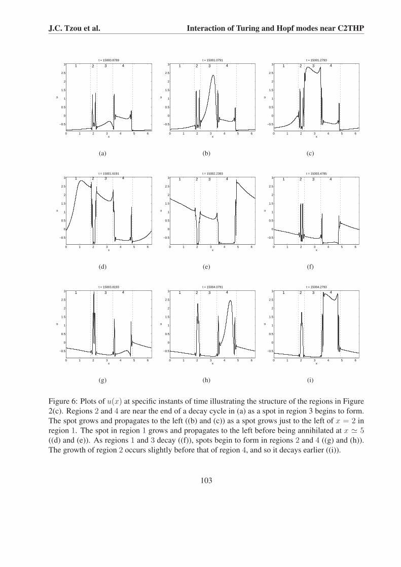
Figure 2(c) shows four dislocations that propagate uniformly in time, with three that propagateto the left, and one that propagates to the right. These dislocations are sites at which a spot is bornon one side and propagates away from it, and another spot generated at an adjacent dislocationis annihilated on the other side. The four dislocations divide the system into four regions and actas boundaries where spots are born and annihilated. The dislocations appear to propagate untilmeeting another dislocation, at which point the two appear to repel each other. The speed of thedislocations (the inverse of the absolute value of the slopes of the dislocations shown in Figure2(c)) appears to be constant in time and the same for all dislocations. The time at which a spot iscreated in one particular region is much closer to the time at which a spot is created in the intervalon the other side of its neighbor. For example, at t = 1.5×104 in Figure 2(c), a spot creation eventin the interval centered at x ' 2 will either be closely preceded or followed by a spot creationevent in the interval centered at x ' 4.1. Figures 6(a) - 6(f) indicate the intervals (labeled 1-4 inthe figures) and illustrate the dynamical behavior within each interval. The figures represent thedynamical evolution of the pattern for times near the lower part of Figure 2(c). Figure 6(a) showsthe two regions centered at x ' 2 (region 2) and x ' 4.1 (region 4) near the end of a decay process,just as a spot has formed in the region centered at x ' 3 (region 3). This spot then grows (Figure6(b)) and propagates to the left (Figure 6(c)) just as a spot begins to form to the left of x = 2 inthe region centered near x ' 0 (region 1). This spot grows and propagates to the left as the spotin region 3 is annihilated and the whole interval begins to decay (Figure 6(d)). The spot in region1 continues to propagate to the left until it is annihilated near x = 5 (Figure 6(e)). As intervals 1and 3 decay, spots begin to form in regions 2 and 4 (Figure 6(f)). The spot in region 2 reaches its

101


1.9 1.95 2 2.05 2.1 2.15

−0.5

0

0.5

1

1.5

2

2.5

t = 15000.8994

x

u

A

B C

(a)

1.9 1.95 2 2.05 2.1 2.15

−0.5

0

0.5

1

1.5

2

2.5

t = 15001.6787

x

u

B CA

(b)

1.9 1.95 2 2.05 2.1 2.15

−0.5

0

0.5

1

1.5

2

2.5

t = 15001.7988

x

u

B C

A

(c)

1.9 1.95 2 2.05 2.1 2.15

−0.5

0

0.5

1

1.5

2

2.5

t = 15002.5391

x

u

B C

A

B’ C’

(d)

1.9 1.95 2 2.05 2.1 2.15

−0.5

0

0.5

1

1.5

2

2.5

t = 15005.999

x

u

A

B’ C’

(e)

Figure 5: Line plots describing details of the right inverted U of Figure 2(b) at specific instants oftime. A spot centered at x ' 2.03 grows at a faster rate than the two oppositely propagating spotscentered at x ' 1.95 and x ' 2.1 ((a) and (b)). In (c), all three spots have achieved values closeto their maximal value, with that of the middle spot being much larger. The three spots then decaytogether, appearing to merge together into one structure ((d)), from which two new spots are bornto replace the two outer spots ((e)).

maximum (Figure 6(g)) before the spot in region 4 forms and propagates to the left (Figure 6(h)and 6(i)). Regions 2 and 4 then decay, and the process starts over again.

With α = β = 1.5 and z = 1.2, the only steady states found using the same initial conditions asthose used for the regular diffusion computations were those of spatially homogeneous oscillations.

For z = 1.4, B = 6.76, and η = 0.642 (Figures 7(a) - 7(f)), we found spatiotemporal patternsfor both the (α, β) = (1.5, 1.5) and (2, 2) cases. Figures 7(a) and 7(d) correspond to the sameinitial conditions, only the diffusion coefficients differ ((α, β) = (1.5, 1.5) and (2, 2) respectively),similarly for Figures 7(b) and 7(e) and Figures 7(c) and 7(f).

Figure 7(a) resembles Figure 2(a) in that the apparently horizontal lines are slightly U-shaped.The stripes for the anomalous case, however, do not breathe as do those in the regular diffusion

102


0 1 2 3 4 5 6

−0.5

0

0.5

1

1.5

2

2.5

3t = 15000.8789

x

u

1 2 3 4

(a)

0 1 2 3 4 5 6

−0.5

0

0.5

1

1.5

2

2.5

3t = 15001.0791

x

u

1 2 3 4

(b)

0 1 2 3 4 5 6

−0.5

0

0.5

1

1.5

2

2.5

3t = 15001.2793

x

u

1 2 3 4

(c)

0 1 2 3 4 5 6

−0.5

0

0.5

1

1.5

2

2.5

3t = 15001.6191

x

u

32 41

(d)

0 1 2 3 4 5 6

−0.5

0

0.5

1

1.5

2

2.5

3t = 15002.2393

x

u

1 2 3 4

(e)

0 1 2 3 4 5 6

−0.5

0

0.5

1

1.5

2

2.5

3t = 15003.4785

x

u

1 2 3 4

(f)

0 1 2 3 4 5 6

−0.5

0

0.5

1

1.5

2

2.5

3t = 15003.8193

x

u

1 3 4

(g)

0 1 2 3 4 5 6

−0.5

0

0.5

1

1.5

2

2.5

3t = 15004.0791

x

u

1 2 3 4

(h)

0 1 2 3 4 5 6

−0.5

0

0.5

1

1.5

2

2.5

3t = 15004.2793

x

u

1 2 3 4

(i)

Figure 6: Plots of u(x) at specific instants of time illustrating the structure of the regions in Figure2(c). Regions 2 and 4 are near the end of a decay cycle in (a) as a spot in region 3 begins to form.The spot grows and propagates to the left ((b) and (c)) as a spot grows just to the left of x = 2 inregion 1. The spot in region 1 grows and propagates to the left before being annihilated at x ' 5((d) and (e)). As regions 1 and 3 decay ((f)), spots begin to form in regions 2 and 4 ((g) and (h)).The growth of region 2 occurs slightly before that of region 4, and so it decays earlier ((i)).

103


(a) (b) (c)

(d) (e) (f)

Figure 7: Spatiotemporal patterns of u for α = β = 1.5 ((a), (b), (c)) and α = β = 2 ((d), (e),(f)), with z = 1.4, B = 6.76, and η = 0.642. Each pair (a) and (d), (b) and (e), and (c) and(f) are generated from the same set of random initial conditions. As with Figure 2, most of thepatterns for this parameter set have low spatial frequency and are mainly time-oscillatory. Themain difference is in the presence of the inverted U’s of the regular diffusion figures versus the flatoscillatory structures of the anomalous figures.

case. Comparing Figures 7(a) and 7(d), we see that for the regular diffusion case, instead of therebeing a spot created away from the stripes that splits into two spots that are annihilated on eitherside of the stripes (U-shape), two spots are generated on either side of the stripes, which thenoppositely propagate and are annihilated between the generation sites, resulting in an inverted U-shape. In Figure 7(d), the left spot fires first, resulting in an annihilation site that is closer to theright side of the stripes than to the left. Thus, for the anomalous case, there is creation away fromthe stripes and annihilation at the stripes (U-shaped), while for regular diffusion, there is creationat the stripes and annihilation away from the stripes (inverted U).

Figure 7(b) (anomalous) shows a single traveling dislocation that propagates to the right. Peri-odically, a spot is generated on the left side of the dislocation, which then propagates until it hitsthe right side of the dislocation. This steady state is similar to but simpler than the pattern in Figure

104


2(c). There are three periods associated with this steady state: the time it takes for a newly formedspot to travel from one side of the dislocation to the other (∼ 1.08 time units), the time betweentwo spot-creation events (∼ 5.2092 time units), and the time it takes for the dislocation to travelone length of the system (∼ 939.039 time units). None of the ratios computed from these periodsappear to be a simple rational number. While all results of the computation are necessarily rational,this suggests that in reality the periods are incommensurate, a situation that can lead to chaos, butdoes not seem to do so in this case. Figure 7(c) is similar to Figure 7(a), the only difference beingthe number of stripes. Figures 7(d) and 7(e) appear to be the same solution modulo a shift in space.

In Figure 7(f), unlike in Figure 7(d), all spots appear to fire simultaneously. The small invertedU’s embedded in the stripes are similar to those found in Figure 2(b). The dynamical behavior ofone of the larger inverted U’s centered at x ' 3.2 of Figure 7(f) is illustrated in more detail inFigures 8(a) - 8(d), where u is plotted against x for a restricted x interval. They correspond to theinverted U that occurs between t = 1.5005 × 104 and t = 1.501 × 104. Figure 8(a) shows theformation of two spots A and B. They co-propagate and grow (Figure 8(b)) before meeting andannihilating in the middle while two new spots are formed in their place (Figures 8(c) and 8(d)).The new spots are labeled A′ and B′ in Figure 8(d).

Figures 9(a) - 9(c) show spatiotemporal patterns of single or multiple localized structures in asea of stripes for α = β = 1.5, z = 1.6, B = 7.76 and η = 0.67. Figure 9(d) is a close-up ofFigure 9(c). Using the same initial conditions, only stationary stripes were found for the case ofregular diffusion.

The predominant structures seen for this parameter set are the square-shaped spatiotemporalcells that take on the shape of an inverted U with a flat apex, which we did not find for regulardiffusion. It appears that, depending on the initial conditions, these cells can occur in differentsizes and numbers, and can have any relative spacing between them. Some square cells behavein a similar fashion as the inverted U’s of Figure 7(f) in that a small spot arises rapidly betweentwo slowly growing and oppositely propagating spots, which are subsequently absorbed into theinterior spot. However, there are some significant differences described below. For some squarecells this is a spatially symmetric process that results in a concentrated bright spot at the apex.Other square cells can exhibit either symmetric or slightly asymmetric behavior. In either case,the interior spot is much wider and is less localized than that of the inverted U’s in Figure 2(b),accounting for the absence of a bright spot at the apex.

Figures 10(a)-10(d) illustrate the detailed dynamics of the symmetric square cell shown inFigure 9(c) (closeup in Figure 9(d)). These figures are plotted only over a restricted x intervalcorresponding to the extent of the square cell. An interior spot (spot A in Figures 10(a) and 10(b))grows in the middle of two oppositely propagating spots (spots B and C in Figures 10(a) and 10(b)).Spot A then splits into two counter propagating spots (spots D and E in Figure 10(c)), which mergewith spots B and C (Figure 10(c)). The solution over the entire interval then decays as two newspots form at the edge of the square cells to replace spots B and C (spots B′ and C′ in Figure10(d)). The process then repeats periodically. The primary difference between these patterns andthe inverted U’s found with regular diffusion, e.g., Figure 2(b), is that the interior spot splits intotwo rapidly counter propagating spots over such a rapid timescale that the apex appears flat andthe interval of the cell appears to “fire” as one (essentially flat) unit.

105


2 2.5 3 3.5 4 4.5−1

−0.5

0

0.5

1

1.5

2

2.5

3

3.5

t = 15004.8789

x

uA B

(a)

2 2.5 3 3.5 4 4.5−1

−0.5

0

0.5

1

1.5

2

2.5

3

3.5

t = 15005.2793

x

u

A B

(b)

2 2.5 3 3.5 4 4.5−1

−0.5

0

0.5

1

1.5

2

2.5

3

3.5

t = 15006.7988

x

u

C

(c)

2 2.5 3 3.5 4 4.5−1

−0.5

0

0.5

1

1.5

2

2.5

3

3.5

t = 15010.1191

x

u

A’ B’

(d)

Figure 8: Line plots describing details of the spatiotemporal cell centered at x ' 3.2 in Figure 7(f).Two spots are created at the stripes ((a)), which then co-propagate and grow ((b)) before meetingand annihilating in the middle while two new spots are formed in their place ((c) and (d)).

In an asymmetric square cell, (e.g., the cell centered at x ' 5.3 in Figure 9(a)), either a spotforms closer to one of the oppositely propagating spots, or one of the oppositely propagating spotsitself grows and propagates more quickly. The dynamics of this square cell exhibiting the latterscenario is illustrated in Figures 11(a)-11(d). A growing spot (spot B in Figure 11(a) and 11(b))propagates toward the more slowly growing spot (spot A). The two spots then merge leading to anasymmetric structure (Figure 11(d)).

We next consider the effect of deterministic initial conditions. Figures 12(a) - 12(g) are gener-ated using u = cos mx and v = sin mx for various m as initial conditions. All other parameters arethe same for all of the figures and are the same as the parameters employed in Figures 9(a)-9(c).For m = 1, . . . , 10, in cases when we found spatiotemporal cells (when m = 1, 2, 3, 4, 5, 8, 9),aside from the two cells in the m = 1 case (Figure 12(a)), the number of square cells was equal tom. The square cells were all uniformly spaced, symmetric and of the same size. For m = 6, 7, 10,we found stationary stripes. For m > 10 we have only computed for m = 60 and m = 180 which

106


(a) (b)

(c) (d)

Figure 9: Spatiotemporal patterns of u for anomalous diffusion with α = β = 1.5, z = 1.6,B = 7.76 and η = 0.67. The figures differ only in initial condition. Compared to Figures 2(a)-2(c) and Figures 7(a) - 7(f), these figures show a more Turing-dominant structure in which time-oscillatory structures are embedded. (d) is a close-up of the spatiotemporal cell of (c). Dependingon the initial conditions, the spatiotemporal cells can occur in any size, number, and with anyrelative spacing.

yielded pure Hopf (horizontal stripes) and pure Turing (stationary vertical stripes), respectively.The individual square cells are similar to the symmetric square cells obtained for random initial

conditions, e.g., Figure 9(c). The primary effect of the deterministic initial conditions is that thesteady state involves uniformly spaced and equal sized square cells. The effect of sinusoidal initialdata for regular diffusion was similar, as in most cases we obtained cells equal in number to m. Insome cases, we obtained identical evenly spaced cells that were either symmetric or asymmetric,depending on the value of m. In other cases, the cells differed in size,were not evenly spaced, anddiffered in number from m. For certain values of m, we also obtained breathing stripes. In allcases, the apex of all cells had a marked inverted U shape, in contrast to the cells with flat apexesobtained in the anomalous case.

In summary, for all three (α, β) pairs, stationary stripe patterns were observed for small z,

107


3.2 3.4 3.6 3.8 4 4.2 4.4

−1

0

1

2

3

4

t = 15003.8594

x

u

A

B C

(a)

3.2 3.4 3.6 3.8 4 4.2 4.4

−1

0

1

2

3

4

t = 15004.1191

x

u

CB

A

(b)

3.2 3.4 3.6 3.8 4 4.2 4.4

−1

0

1

2

3

4

t = 15004.2988

x

u

D E

(c)

3.2 3.4 3.6 3.8 4 4.2 4.4

−1

0

1

2

3

4

t = 15005.4395

x

u

C’B’

(d)

Figure 10: Line plots describing details of the symmetric spatiotemporal cell of Figure 9(d) atspecific instants of time. A spot is created in between two oppositely propagating spots ((a) and (b),which splits into two counter propagating spots that are annihilated with the oppositely propagatingspots (c). Two new spots are formed to replace the two oppositely propagating spots (d).

followed by mainly spatially homogeneous oscillations (horizontal stripes) for larger z. In the caseof (α, β) = (1.1, 1.1), the steady states returned to stationary stripes as z was increased. In thecase of (α, β) = (1.5, 1.5) and (2, 2), steady states with spatiotemporal patterns were observed asz was increased before the steady states returned to mainly stationary stripes.

Spatiotemporal patterns were observed with (α, β) = (2, 2) for z = 1.2 and 1.4, while for(α, β) = (1.5, 1.5), they were observed for z = 1.4, 1.6, and 1.8 (the z = 1.8 case yieldednothing that had not been seen with z = 1.4 and z = 1.6 and is not shown). For both regularand anomalous diffusion there seem to be a large number of stable steady states, as in virtually allcases different initial conditions gave different steady states. In both cases, as z was increased, thesteady states became more stripe-dominated, while for the same z, regular diffusion yielded morestripe-dominated steady states.

In general, patterns obtained with regular diffusion were more diverse, as breathing stripes

108


4.8 5 5.2 5.4 5.6 5.8

−1

0

1

2

3

4

t = 15002.9395

x

u

A B

(a)

4.8 5 5.2 5.4 5.6 5.8

−1

0

1

2

3

4

t = 15003.1592

x

u

B

A

(b)

4.8 5 5.2 5.4 5.6 5.8

−1

0

1

2

3

4

t = 15003.2188

x

u

BA

(c)

4.8 5 5.2 5.4 5.6 5.8

−1

0

1

2

3

4

t = 15003.3594

x

u

(d)

Figure 11: Line plots describing details of an asymmetric spatiotemporal cell of Figure 9(a) cen-tered at x ' 5.3 at specific instants of time. Spot B grows and propagates more quickly than spotA ((b) and (c)) so that the spots merge at a location closer to spot A ((d)).

(Figure 2(a)), inverted U’s with a pronounced peak (Figure 2(b)), multiple traveling dislocations(Figure 2(c)), and inverted U’s (Figure 7(d)) were not observed for anomalous diffusion. Foranomalous diffusion, the predominant pattern appears to be that of spatiotemporal cells in the shapeof inverted U’s with a square apex, embedded in a mainly Turing structure of vertical stripes. Thisis something that we did not find with regular diffusion. With random initial data, the cells occurin different sizes and numbers, and stable steady states with essentially any inter-cell spacing andnumber of cells appear possible.

For sinusoidal initial conditions with wave number m only steady states with symmetric anduniformly spaced cells (with flat apexes) were found. With m = O(1) the resulting steady statehad exactly m cells with the exceptions described above. For larger values of m, only pure Turingand pure Hopf steady states were found. In the case of regular diffusion, breaks in the symmetry ofthe steady states were observed, as described above, and the number of cells was not always equalto m.

109


(a) (b) (c) (d)

(e) (f) (g)

Figure 12: Spatiotemporal patterns of u for anomalous diffusion with α = β = 1.5, z = 1.6,B = 7.76 and η = 0.67. Initial conditions were u = cos mx, v = sin mx with (a) m = 1, (b)m = 2, (c) m = 3, (d) m = 4, (e) m = 5, (f) m = 8, and (g) m = 9. With the exception of (a), thenumber of spatiotemporal cells is equal to m and all cells in each figure are of the same size andspaced evenly, and also oscillate in phase. For m = 1, the number of cells is 2m = 2, and whilethe cells are spaced evenly, they are not equal in size and oscillate out of phase.

5.2 The fully nonlinear regime with unequal diffusion exponentsWe next consider the case α 6= β. In this case s is no longer equal to 1 so that for the same value ofz the values of Bcr and ηc are slightly different from the α = β case. Since we do not change thevalues of µ and η2, both B and η change as a result of the unequal diffusion exponents. To keepthese parameters from changing would require altering how far the system is into the nonlinearregime as well as its closeness to the C2THP, and this could result in a significant qualitativechange in the patterns not attributable to unequal diffusion exponents.

We first kept β = 1.5 while setting α to 1.4 and then to 1.6. For each α, we computedsteady states starting from three sets of initial conditions: the same random initial conditions usedin Section 5.1, the same sinusoidal initial conditions used in Section 5.1, and the steady statescomputed from random initial conditions with α = β = 1.5 and z = 1.6. In this last case, we tookthe solutions u(x) and v(x) at t = 1.5 × 104 and set them as initial conditions for computationswith the same z and different α.

For α = 1.6, β = 1.5, and z = 1.6 (B = 8.57, η = 0.672), the only steady states we foundwere stationary stripes. In contrast, for α = 1.4, β = 1.5 we did find spatiotemporal patterns.

110


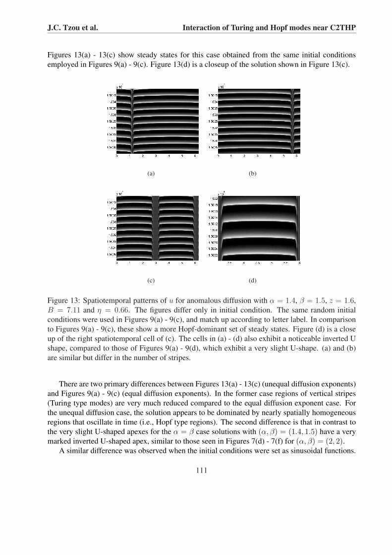
Figures 13(a) - 13(c) show steady states for this case obtained from the same initial conditionsemployed in Figures 9(a) - 9(c). Figure 13(d) is a closeup of the solution shown in Figure 13(c).

(a) (b)

(c) (d)

Figure 13: Spatiotemporal patterns of u for anomalous diffusion with α = 1.4, β = 1.5, z = 1.6,B = 7.11 and η = 0.66. The figures differ only in initial condition. The same random initialconditions were used in Figures 9(a) - 9(c), and match up according to letter label. In comparisonto Figures 9(a) - 9(c), these show a more Hopf-dominant set of steady states. Figure (d) is a closeup of the right spatiotemporal cell of (c). The cells in (a) - (d) also exhibit a noticeable inverted Ushape, compared to those of Figures 9(a) - 9(d), which exhibit a very slight U-shape. (a) and (b)are similar but differ in the number of stripes.

There are two primary differences between Figures 13(a) - 13(c) (unequal diffusion exponents)and Figures 9(a) - 9(c) (equal diffusion exponents). In the former case regions of vertical stripes(Turing type modes) are very much reduced compared to the equal diffusion exponent case. Forthe unequal diffusion case, the solution appears to be dominated by nearly spatially homogeneousregions that oscillate in time (i.e., Hopf type regions). The second difference is that in contrast tothe very slight U-shaped apexes for the α = β case solutions with (α, β) = (1.4, 1.5) have a verymarked inverted U-shaped apex, similar to those seen in Figures 7(d) - 7(f) for (α, β) = (2, 2).

A similar difference was observed when the initial conditions were set as sinusoidal functions.

111


Figures 14(a) - 14(j) show more Hopf-dominated steady states than do Figures 12(a) - 12(g), whichcorrespond to steady states with α = β = 1.5. Further, unlike the α = β = 1.5 case, spatiotempo-ral patterns were obtained for sinusoidal initial conditions of all wave numbers m = 1, . . . , 10.

(a) (b) (c)

(d) (e) (f) (g)

(h) (i) (j)

Figure 14: Spatiotemporal patterns of u for anomalous diffusion with α = 1.4, β = 1.5, z = 1.6,B = 7.11 and η = 0.66. Initial conditions were u = cos mx, v = sin mx with (a) m = 1, (b)m = 2, (c) m = 3, (d) m = 4, (e) m = 5, (f) m = 6, (g) m = 7, (h) m = 8, (i) m = 9, and (j)m = 10. Unlike in Figure 12(a), the m = 1 case ((a)) contains only one spatiotemporal cell. (b) -(d) contain pairs of cells equal in number to m. In (b), the two smaller cells oscillate in phase witheach other, as do the two larger cells. All cells in all other figures are of equal size and oscillatein phase. In (e) - (j), the trend is the same as in the case of equal diffusion exponents in that thenumber of cells is equal to m.

As in the case with equal diffusion exponents, the m = 1 case (Figure 14(a)) appears to be an

112


exception. For m = 2, 3, 4 (Figures 14(b) - 14(d)), we see m pairs of cells so that the total numberof cells is 2m. This is in contrast to the m = 1 case for which there is only one square cell. Thisis also in contrast to the case of equal diffusion exponents, where generally the number of squarecells was m, not 2m. This suggests that the cells split as β − α increases from zero. The m = 2case is also an exception in that there are cells of unequal size that oscillate with a phase difference.In all other cases, the cells are of equal size and oscillate in phase. In Figures 14(e) - 14(j) we donot find cell splitting and the number of cells equals m, similar to the α = β case.

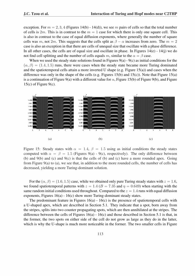
When we used the steady state solutions found in Figures 9(a) - 9(c) as initial conditions for the(α, β) = (1.4, 1.5) runs, there were cases when the steady state became more Turing dominatedand the spatiotemporal cells attain a more inverted U shape (e.g. Figure 15(a)) and cases when thedifference was only in the shape of the cells (e.g. Figures 15(b) and 15(c)). Note that Figure 15(a)is a continuation of Figure 9(a) with a different value for α, Figure 15(b) of Figure 9(b), and Figure15(c) of Figure 9(c).

(a) (b) (c)

Figure 15: Steady states with α = 1.4, β = 1.5 using as initial conditions the steady statescomputed with α = β = 1.5 (Figures 9(a) - 9(c), respectively). The only difference between(b) and 9(b) and (c) and 9(c) is that the cells of (b) and (c) have a more rounded apex. Goingfrom Figure 9(a) to (a), we see that, in addition to the more rounded cells, the number of cells hasdecreased, yielding a more Turing-dominant solution.

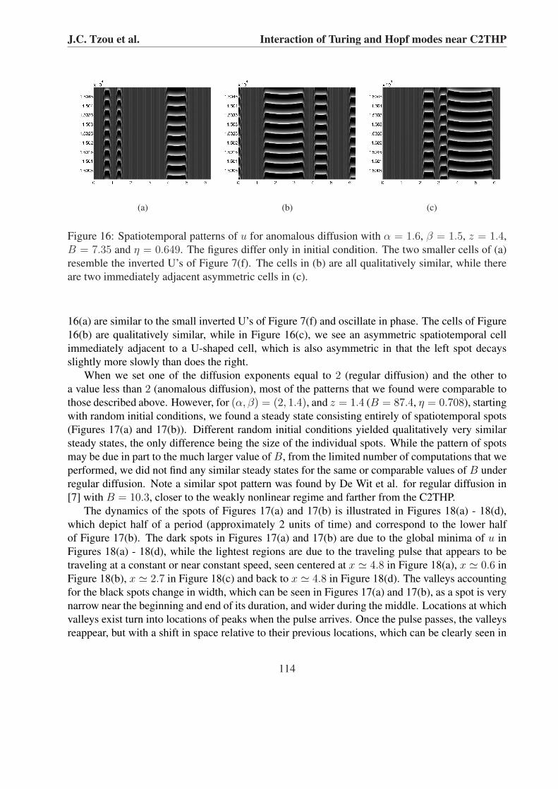
For the (α, β) = (1.6, 1.5) case, while we obtained only pure Turing steady states with z = 1.6,we found spatiotemporal patterns with z = 1.4 (B = 7.35 and η = 0.649) when starting with thesame random initial conditions used throughout. Compared to the z = 1.4 runs with equal diffusionexponents, Figures 16(a) - 16(c) show more Turing-dominant steady states.

The predominant feature in Figures 16(a) - 16(c) is the presence of spatiotemporal cells witha U-shaped apex, which are described in Section 5.1. They indicate that a spot, born away fromthe stripes, splits into two counter propagating spots, which are then annihilated at the stripes. Thedifference between the cells of Figures 16(a) - 16(c) and those described in Section 5.1 is that, inthe former, the two spots on either side of the cell do not grow as large as they do in the latter,which is why the U-shape is much more noticeable in the former. The two smaller cells in Figure

113


(a) (b) (c)

Figure 16: Spatiotemporal patterns of u for anomalous diffusion with α = 1.6, β = 1.5, z = 1.4,B = 7.35 and η = 0.649. The figures differ only in initial condition. The two smaller cells of (a)resemble the inverted U’s of Figure 7(f). The cells in (b) are all qualitatively similar, while thereare two immediately adjacent asymmetric cells in (c).

16(a) are similar to the small inverted U’s of Figure 7(f) and oscillate in phase. The cells of Figure16(b) are qualitatively similar, while in Figure 16(c), we see an asymmetric spatiotemporal cellimmediately adjacent to a U-shaped cell, which is also asymmetric in that the left spot decaysslightly more slowly than does the right.

When we set one of the diffusion exponents equal to 2 (regular diffusion) and the other toa value less than 2 (anomalous diffusion), most of the patterns that we found were comparable tothose described above. However, for (α, β) = (2, 1.4), and z = 1.4 (B = 87.4, η = 0.708), startingwith random initial conditions, we found a steady state consisting entirely of spatiotemporal spots(Figures 17(a) and 17(b)). Different random initial conditions yielded qualitatively very similarsteady states, the only difference being the size of the individual spots. While the pattern of spotsmay be due in part to the much larger value of B, from the limited number of computations that weperformed, we did not find any similar steady states for the same or comparable values of B underregular diffusion. Note a similar spot pattern was found by De Wit et al. for regular diffusion in[7] with B = 10.3, closer to the weakly nonlinear regime and farther from the C2THP.

The dynamics of the spots of Figures 17(a) and 17(b) is illustrated in Figures 18(a) - 18(d),which depict half of a period (approximately 2 units of time) and correspond to the lower halfof Figure 17(b). The dark spots in Figures 17(a) and 17(b) are due to the global minima of u inFigures 18(a) - 18(d), while the lightest regions are due to the traveling pulse that appears to betraveling at a constant or near constant speed, seen centered at x ' 4.8 in Figure 18(a), x ' 0.6 inFigure 18(b), x ' 2.7 in Figure 18(c) and back to x ' 4.8 in Figure 18(d). The valleys accountingfor the black spots change in width, which can be seen in Figures 17(a) and 17(b), as a spot is verynarrow near the beginning and end of its duration, and wider during the middle. Locations at whichvalleys exist turn into locations of peaks when the pulse arrives. Once the pulse passes, the valleysreappear, but with a shift in space relative to their previous locations, which can be clearly seen in

114


(a) (b)

Figure 17: Spatiotemporal patterns of u for anomalous diffusion with (α, β) = (2, 1.4), z = 1.4,B = 87.4, and η = 0.708. (b) shows a closeup of the bottom portion of (a).

Figure 17(a). The result in the space-time plot is that one row of spots runs diagonally, and a rowis displaced by one spot’s width relative to a neighboring row. Over one full period (approximately4 units of time), the valleys return to the same locations.

In summary, it appeared that the (α, β) = (1.4, 1.5) steady states with z = 1.6 were moreHopf-dominant than the cases with (α, β) = (1.5, 1.5). In the case of the continuation runs,however, this trend was not seen. In the case of (α, β) = (1.6, 1.5) with z = 1.4, the steadystates appeared to be more Turing-dominant than the same runs with (α, β) = (1.5, 1.5). Thistrend seems more consistent, as pure Turing steady states were found for z = 1.6 for all initialconditions mentioned above. Further, the spatiotemporal cells, which appear to have a flat apexin the (α, β) = (1.5, 1.5) case, take on an inverted U shape in the (α, β) = (1.4, 1.5) case anda U-shape in the (α, β) = (1.6, 1.5) case. In the case when one component undergoes regulardiffusion and the other anomalous, we found a series of adjacent valleys that periodically turn intopeaks when a traveling pulse arrives, accounting for the dark spots and their arrangement in Figure17(a). Similar structures were found for regular diffusion in [7].

Since in all of these cases, B and η change as described above it is difficult to infer whetherthese differences are due solely to the difference in diffusion exponents.

6 ConclusionsUsing weakly nonlinear analysis, we derived a pair of coupled amplitude equations that describethe evolution of the Turing and Hopf modes over a long time scale near a C2THP of the superdif-fusive Brusselator model. The amplitude equations have a similar form to those of the regularmodel, but differ in three regards: the two spatial derivatives in the pair of equations are withrespect to two different length scales, the equation describing the evolution of the Hopf mode con-tains an integro-differential operator, which reflects the non-local effect of anomalous diffusion,

115


and finally, the coefficients of the amplitude equations differ from those of the regular amplitudeequations. The latter two differences contribute to the differences in the long wave stability criteriaof the special solutions, which are described in Section 4. Two of these criteria were confirmedwith numerical computations in the weakly nonlinear regime, while criteria involving both theTuring and Hopf modes were inconclusive due to numerical difficulties arising from small ε.

0 1 2 3 4 5 6−6

−4

−2

0

2

4

6

8

t = 15000.0586

x

u

(a)

0 1 2 3 4 5 6−6

−4

−2

0

2

4

6

8

t = 15000.7793

x

u(b)

0 1 2 3 4 5 6−6

−4

−2

0

2

4

6

8

t = 15001.4189

x

u

(c)

0 1 2 3 4 5 6−6

−4

−2

0

2

4

6

8

t = 15002.0791

x

u

(d)

Figure 18: Line plots describing details of the spots of Figures 17(a) and 17(b) at specific instantsof time. The global minima, account for the dark spots in Figures 17(a) and 17(b).

In computations in the fully nonlinear regime, one of the dominant spatiotemporal structuresthat we found under anomalous diffusion were the square-shaped spatiotemporal cells with eithera flat apex (α = β), an inverted U shaped apex (α < β), or a U-shaped apex (α > β). Qualitativelysimilar structures were found under regular diffusion with a similar range in values of z, thoughthe square and flat cells embedded in a mainly Turing structure was something that we did not findunder regular diffusion. There was also behavior that we found under regular diffusion that wedid not find with anomalous diffusion, such as breathing stripes and multiple traveling dislocationsthat appear to repel each other. With equal diffusion exponents, it appeared that the effect ofanomalous diffusion was to delay the onset of Hopf-type behavior in terms of increasing z, and

116


also to inhibit spatiotemporal pattern formation, as was seen when we found only pure Turing andpure Hopf solutions with α = β = 1.1. The main effect of unequal but close diffusion exponentsappeared to be to alter the apex shape of the spatiotemporal cells from the case of equal diffusionexponents. When one diffusion was regular and the other anomalous, we found spatiotemporalspots corresponding to valleys whose sizes and positions changed periodically, similar to structurespresented in [7]. More generally, we found a large number of steady state patterns consistingof a localized region or regions of stationary stripes in a background of time periodic cellularmotion, as well as a localized region or regions of time periodic cells in a background of stationarystripes. Each such pattern lies on a branch of such solutions, is stable and corresponds to a differentinitial condition. The patterns correspond to the phenomenon of pinning of the front between thestripes and the time periodic cellular structure. The different branches live in a region called thepinning region in which such solution branches snake back and forth. The idea of pinning wasoriginally suggested by Pomeau [13], who referred to pinning as locking. The idea has beenconsidered and extended by a number of researchers, including Knobloch and coauthors [1, 3, 4],who considered localized stationary patterns in a background of a stationary, spatially uniformstate, as well as in a background of small amplitude traveling waves, Bensimon et. al. [2], whoconsidered localized traveling rolls (stripes) in a background of a stationary, spatially uniform state,and Malomed et. al [9], who considered localized hexagonal patterns in a background of stationarystripes. These scenarios involve a subcritical bifurcation leading to bistability between the basicstate and the bifurcated state after the latter turns around to become stable. In contrast, our studyinvolves bistability between two stable supercritical branches which exist near a codimension twobifurcation point. We note that many of these patterns disappear when the size L of the domain isconsiderably reduced.

AcknowledgmentsThe authors gratefully acknowledge the support of U.S. National Science Foundation grant DMS0707445 and Natural Sciences and Engineering Research Council of Canada grant PGS D - 358595- 2009.

References[1] P. Assemat, A. Bergeon, E. Knobloch. Spatially localized states in Marangoni convection

in binary mixtures. Fluid Dynamics Research 40 (2008), 852-876.

[2] D. Bensimon, B.I. Shraiman, V. Croquette. Nonadiabatic effects in convection. Phys. Rev.A38 (1988), 5461-5464.

[3] J. Burke, E. Knobloch. Localized states in the generalized Swift-Hohenberg equation. Phys.Rev. E73 (2006), art. 56211.

117


[4] J. Burke, E. Knobloch. Homoclinic snaking: structure and stability Chaos 17 (2007), art.037102.

[5] E.J. Crampin, E.A. Gaffney, P.K. Maini. Reaction and diffusion on growing domains:Scenarios for robust pattern formation. Bull. Math. Biol., 61 (1999), 1093-1120.

[6] A. De Wit. Spatial patterns and spatiotemporal dynamics in chemical systems. Adv. Chem.Phys., 109 (1999), 435–513.

[7] A. De Wit, D. Lima, G. Dewel, P. Borckmans. Spatiotemporal dynamics near a codimension-two point. Phys. Rev. E54 (1996), 261–271.

[8] A.A. Golovin, B.J. Matkowsky, V.A. Volpert. Turing pattern formation in the Brusselatormodel with superdiffusion. SIAM J. Appl. Math., 69 (2008), 251–272.

[9] B.A. Malomed, A.A. Nepomnyashchy, M.I. Tribelsky. Domain boundaries in convectionpatterns. Phys. Rev. A42 (1990), 7244-7263.

[10] R. Metzler, J. Klafter. The random walk’s guide to anomalous diffusion: a fractional dynam-ics approach. Phys. Rep. 339 (2000), No. 1, 1–77.

[11] Y. Nec, A.A. Nepomnyashchy, A.A. Golovin. Oscillatory instability in super-diffusivereaction-diffusion systems: Fractional amplitude and phase diffusion equations. EPL, 82(2008), 58003 (6pp).

[12] K.B. Oldham, J. Spanier. The fractional calculus. Academic Press, New York, 1974.

[13] Y. Pomeau. Front motion, metastability and subcritical bifurcations in hydrodynamics. Phys-ica D23 (1986), 3-11.

[14] J.C. Tzou, B.J. Matkowsky, V.A. Volpert. Interaction of Turing and Hopf modes in the su-perdiffusive Brusselator model. Appl. Math. Lett. 22 (2009), 1432–1437.

[15] L. Yan, M. Dolnik, A.M. Zhabotinsky, I.R. Epstein. Pattern formation arising from interac-tion between Turing and wave instabilities. J. Chem. Phys., 117 (2002), 7259–7265.

118

Date post:	21-Jun-2018
Category:	Documents
Upload:	truongduong
View:	213 times
Download:	0 times

Interaction of Turing and Hopf Modes in the Superdiffusive...

Documents