Interactions of Visual Attention and Object Recognition: Computational Modeling, Algorithms, and Psychophysics Thesis by Dirk Walther In Partial Fulfillment of the Requirements for the Degree of Doctor of Philosophy California Institute of Technology Pasadena, California 2006 (Submitted March 7, 2006)
Transcript
Interactions of Visual Attention and Object Recognition:Computational Modeling, Algorithms, and Psychophysics
Figure 2.2: Illustration of the processing steps for obtaining the attended region. The input imageis processed for low-level features at multiple scales, and center-surround differences are computed(eq. 2.3). The resulting feature maps are combined into conspicuity maps (eq. 2.6) and, finally, intoa saliency map (eq. 2.7). A winner-take-all neural network determines the most salient location,which is then traced back through the various maps to identify the feature map that contributesmost to the saliency of that location (eqs. 2.8 and 2.9). After segmentation around the most salientlocation (eqs. 2.10 and 2.11), this winning feature map is used for obtaining a smooth object maskat image resolution and for object-based inhibition of return.
10
2.3 Attending Proto-object Regions
While Itti et al.’s model successfully identifies the most salient location in the image, it has no
notion of the extent of the attended object or object part at this location. We introduce a method
of estimating this region based on the maps and salient locations computed so far, using feedback
connections in the saliency computation hierarchy (figure 2.2). Looking back at the conspicuity
maps, we find the one map that contributes the most to the activity at the most salient location:
kw = argmaxk∈{I,C,O}
Ck(xw, yw). (2.8)
The argmax function, which is critical to this step, could be implemented in a neural network of
linear threshold units (LTUs), as shown in figure 2.3. For practical applications we use a more
efficient generic argmax function because of its higher efficiency.
Examining the feature maps that gave rise to the conspicuity map Ckw, we find the one that
contributes most to its activity at the winning location:
(lw, cw, sw) = argmaxl∈Lkw ,c∈{2,3,4},s∈{c+3,c+4}
Fl,c,s(xw, yw), (2.9)
with Lkwas defined in eqs. 2.4. The “winning” feature map Flw,cw,sw
(figure 2.2) is segmented
around (xw, yw). For this operation, a binary version of the map (B) is obtained by thesholding
Flw,cw,sw with 1/10 of its value at the attended location:
B(x, y) =
1 if Flw,cw,sw(x, y) ≥ 0.1 · Flw,cw,sw(xw, yw)
0 otherwise. (2.10)
The 4-connected neighborhood of active pixels in B is used as the template to estimate the spatial
extent of the attended object:
Fw = label (B, (xw, yw)) . (2.11)
For the label function, we use the classical algorithm by Rosenfeld and Pfaltz (1966) as implemented
in the Matlab bwlabel function. After a first pass over the binary map for assigning temporary
labels, the algorithm resolves equivalence classes and replaces the temporary labels with equivalence
class labels in a second pass. In figure 2.4 we show an implementation of the segmentation operation
with a network of LTUs to demonstrate feasibility of our procedure in a neural network. The
segmented feature map Fw is used as a template to trigger object-based inhibition of return (IOR)
in the WTA network and to deploy spatial attention to subsequent processing stages such as object
detection.
We have implemented our model of salient region selection as part of the SaliencyToolbox for
Figure 2.3: A network of linear threshold units (LTUs) for computing the argmax function in eq. 2.8for one image location. Feed-forward (blue) units fCol, fInt, and fOri compute conspicuity maps forcolor, intensity, and orientation by pooling activity from the respective sets of feature maps asdescribed in eqs. 2.5 and 2.6, omitting the normalization step N here for clarity. The saliency mapis computed in a similar fashion in fSM (eq. 2.7), and fSM participates in the spatial WTA competitionfor the most salient location. The feed-back (red) unit bSM receives a signal from the WTA onlywhen this location is attended to, and it relays the signal to the b units in the conspicuity maps.Competition units (c) together with a pool of inhibitory interneurons (black) form an across-featureWTA network with input from the f units of the respective conspicuity maps. Only the most activec unit will remain active due to WTA dynamics, allowing it to unblock the respective b unit. Asa result, the activity pattern of the b units represents the result of the argmax function in eq. 2.8.This signal is relayed further to the constituent feature maps, where a similar network selects thefeature map with the largest contribution to the saliency of this location (eq. 2.9).
12
PS
selectout
map input
PS
PS
PS
PS
PS
PS
PS
PS
inhibitory synapseexcitatory synapse
Figure 2.4: An LTU network implementation of the segmentation operation in eqs. 2.10 and 2.11.Each pixel consists of two excitatory neurons and an inhibitory interneuron. The thresholding oper-ation in eq. 2.10 is performed by the inhibitory interneuron, which only unblocks the segmentationunit S if input from the winning feature map Flw,cw,sw
(blue) exceeds its firing threshold. S can beexcited by a select signal (red) or by input from the pooling unit P. Originating from the feedbackunits b in figure 2.3, the select signal is only active at the winning location (xw, yw). Pooling thesignals from the S unit in its 4-connected neighborhood, P excites its own S unit when it receives atleast one input. Correspondingly, the S unit projects to the P units of the pixels in the 4-connectedneighborhood. In their combination, the reciprocal connections between the S and P units form alocalized implementation of the labeling algorithm (Rosenfeld and Pfaltz 1966). Spreading of acti-vation to adjacent pixels stops where the inbound map activity is not large enough to unblock theS unit. The activity pattern of the S units (green) represents the segmented feature map Fw.
Matlab, described in appendix B, and as part of the iLab Neuromorphic Vision (iNVT) C++
toolkit. In the Matlab toolbox we provide both versions of the segmentation operation, the fast
image processing implementation, and the LTU network version. They are functionally equivalent,
but the LTU network simulation runs much slower than the fast image processing version.
Figure 2.5 shows examples of applying region selection to three natural images as well as an
artificial display of bent paper clips as used for the simulations in chapter 3. These examples and
the results in chapters 3 and 5 were obtained using iNVT toolkit; for chapter 6 we used a modified
version that was derived from the iNVT toolkit; and for chapter 4 we used the SaliencyToolbox.
2.4 Discussion
As part of their selective tuning model of visual attention, Tsotsos et al. (1995) introduced a mecha-
nism for tracing back activations through a hierarchical network of WTA circuits to identify contigu-
ous image regions with similarly high saliency values within a given feature domain. Our method is
13
Figure 2.5: Four examples for salient region extraction as described in section 2.3. For each examplethe following steps are shown (from left to right): the original image I; the saliency map S; theoriginal image contrast-modulated with a cumulative superposition of Fw for the locations attendedto during the first 700 ms of simulated time of the WTA network, with the scan path overlayed; andthe inverse of this cumulative mask, covering all salient parts of the image. It is apparent from thisfigure that our salient region extraction approach does indeed cover the salient parts of the images,leaving the non-salient parts unattended.
similar in spirit but extends across feature domains. By tracing back the activity from the attended
location in the saliency map through the hierarchy of conspicuity and feature maps, we identify
the feature that contributes most to the activity of the currently fixated location. We identify a
contiguous region around this location with high activity in the feature map that codes for this most
active feature. This procedure is motivated by the observation that between-object variability of
visual information is significantly higher than within-object variability (Ruderman 1997). Hence,
even if two salient objects are close to each other or occluding each other, it is not very likely that
they are salient for the same reason. This means that they can be distinguished in the feature maps
that code for their respective most active features.
Note, however, that attended regions may not necessarily have a one-to-one correspondence to
objects. Groups of similar objects, e.g., a bowl of fruits, may be segmented as one region, as may
object parts that are dissimilar from the rest of the object, e.g., a skin-colored hand appearing
to terminate at a dark shirt sleeve. We call these regions “proto-objects” because they can lead
14
to the detection of the actual objects in further iterative interactions between the attention and
recognition systems. See the work by Rybak et al. (1998), for instance, for a model that uses the
vector of saccades to code for the spatial relations between object parts.
The additional computational cost for region selection is minimal because the feature and con-
spicuity maps have already been computed during the processing for saliency. Note that although
ultimately only the winning feature map is used to segment the attended image region, the inter-
action of WTA and IOR operating on the saliency map provides the mechanism for sequentially
attending several salient locations.
There is no guarantee that the region selection algorithm will find objects. It is purely bottom-
up, stimulus driven and has no prior notion of what constitutes an object. Also note that we are
not attempting an exhaustive segmentation of the image, such as done by Shi and Malik (2000) or
Martin et al. (2004). Our algorithm provides us with a first rough guess of the extent of a salient
region. As we will see in the remainder of this thesis, in particular in chapter 5, it works well for
localizing objects in cluttered environments.
In some respects, our method of extracting the approximate extent of an object bridges spatial
attention with object-based attention. Egly et al. (1994), for instance, report spreading of attention
over an object. In their experiments, subjects detected invalidly cued targets faster if they appeared
on the same object than if they appeared on a different object than the cue, although the distance
between cue and target was the same in both cases. In our method, attention spreads over the
extent of a proto-object as well, guided by the feature with the largest contribution to saliency at
the attended location. Finding this most active feature is somewhat similar to the idea of flipping
through an “object file”, a metaphor for a collection of properties that comprise an object (Kahneman
and Treisman 1984). However, while Kahneman and Treisman (1984) consider spatial location of an
object as another entry in the object file, in our implementation spatial location has a central role
as an index for binding together the features belonging to a proto-object. Our method should be
seen as an initial step toward a location invariant object representation, providing initial detection
of proto-object that allow for subsequent tracking or recognition operations. In fact, in chapter 6,
we demonstrate the suitability of our approach as a detection step for multi-target tracking in a
machine vision application.
2.5 Outlook
In this chapter we have introduced our model of bottom-up salient region selection based on the
model of saliency-based bottom-up attention by Itti et al. (1998). The attended region, which is
given by the segmented feature map Fw from eq. 2.11, serves as a means of deploying selective visual
attention for:
15
(i) modulation of neural activity at specific levels of the visual processing hierarchy (chapter 3);
(ii) preferential processing of image regions for learning and recognizing objects (chapter 5);
(iii) initiating object tracking and simplifying the assignment problem in multi-target tracking
(chapter 6).
16
17
Chapter 3
Modeling the Deployment ofSpatial Attention
3.1 Introduction
When looking at a complex scene, our visual system is confronted with a large amount of visual
information that needs to be broken down for processing by the visual system. Selective visual
attention provides a mechanism for serializing visual information, allowing for sequential processing
of the content of the scene. In chapter 2 we explored how such a sequence of attended locations
can be obtained from low-level image properties by bottom-up processes, and in chapter 4 we will
show how top-down knowledge can be used to bias attention toward task-relevant objects. In this
chapter, we investigate how selective attention can be deployed in a biologically realistic manner
in order to serialize the perception of objects in scenes containing several objects (Walther et al.
2002a,b). This work was started under the supervision of Dr. Maximilian Riesenhuber at MIT. I
designed the mechanism for deploying spatial atention to the HMAX object recognition system, and
I conducted the experiments and analyses.
3.2 Model
To test attentional modulation of object recognition, we adopt the hierarchical model of object
recognition by Riesenhuber and Poggio (1999b). While this model works well for individual paper
clip objects, its performance deteriorates quickly when it is presented with scenes that contain several
such objects because of erroneous binding of features (Riesenhuber and Poggio 1999a). To solve this
feature binding problem, we supplement the model with a mechanism of modulating the activity of
the S2 layer, which has roughly the same receptive field properties as area V4, or the S1 layer, whose
properties are similar to simple cells in areas V1 and V2, with an attentional modulation function
obtained from our model for saliency-based region selection described in chapter 2 (figure 3.1). Note
18
µS
2
µS
1
Figure
3.1:Sketch
ofthe
combined
model
ofbottom
-upattention
(left)and
object
recognition(right)
with
attentionalm
odulationat
theS2
orS1
layeras
describedin
eq.3.2.
19
that only the shape selectivity of neurons in V1/V2 and V4, is captured by the model units. Other
aspects such as motion sensitivity of area V1 or color sensitivity of V4 neurons are not considered
here.
3.2.1 Object Recognition
The hierarchical model of object recognition in cortex by Riesenhuber and Poggio (1999b) starts
with S1 simple cells, which extract local orientation information from the input image by convolution
with Gabor filters, for the four cardinal orientations at 12 different scales. S1 activity is pooled over
local spatial patches and four scale bands using a maximum operation to arrive at C1 complex cells.
While still being orientation selective, C1 cells are more invariant to space and scale than S1 cells.
In the next stage, activities from C1 cells with similar positions but different orientation selec-
tivities are combined in a weighted sum to arrive at S2 composite feature cells that are tuned to a
dictionary of more complex features. The dictionary we use in this chapter consists of all possible
combinations of the four cardinal orientations in a 2×2 grid of neurons, i.e., (2×2)4 = 256 different
S2 features. This choice of features limits weights to being binary, and, for a particular location in
the C1 activity maps, the weight for one and only one of the orientations is set to 1. We use more
complex S2 features learned from natural image statistics in chapter 4 (see also Serre et al. 2005b).
The S2 layer retains some spatial resolution, which makes it a suitable target for spatial attentional
modulation detailed in the next section.
In a final non-linear pooling step over all positions and scale bands, activities of S2 cells are
combined into C2 units using the same maximum operation used from the S1 to the C1 layer.
While C2 cells retain their selectivity for the complex features, this final step makes them entirely
invariant to location and scale of the preferred stimulus. The activity patterns of the 256 C2
cells feed into view-tuned units (VTUs) with connection weights learned from exposure to training
examples. VTUs are tightly tuned to object identity, rotation in depth, illumination, and other
object-dependent transformations, but show invariance to translation and scaling of their preferred
object view.
In their selectivity to shape, S1 and C1 layers are approximately equivalent to simple and complex
cells in areas V1 and V2, S2 to area V4, and C2 and the VTUs to areas in posterior inferotemporal
cortex (PIT) with a spectrum of tuning properties ranging from complex features to full object
views.
It should be noted that this is a model of fast feed-forward processing in object detection. The
time course of object detection is not modeled here, which means in particular that such effects
as masking or priming are not explained by the model. In this chapter we introduce feedback
connections for deploying spatial attention, thereby introducing some temporal dynamics due to the
succession of fixation.
20
3.2.2 Attentional Modulation
Attentional modulation of area V4 has been reported in monkey electrophysiology (Moran and
Desimone 1985; Reynolds et al. 2000; Connor et al. 1997; Motter 1994; Luck et al. 1997; McAdams
and Maunsell 2000; Chelazzi et al. 2001) as well as human psychophysics (Intriligator and Cavanagh
2001; Braun 1994). Other reports find attentional modulation in area V1 using fMRI in humans
(Kastner et al. 1998; Gandhi et al. 1999) and electrophysiology in macaques (McAdams and Reid
2005). There are even reports of the modulation of fMRI activity in LGN due to selective attention
(O’Connor et al. 2002). See figure 3.6 for an overview of attentional modulation of V4 units in
electropysiology work in macaques.
Here we explore attentional modulation of layers S2 and S1, which correspond approximately to
areas V4 and V1, by gain modulation with variable modulation strength. We use the bottom-up
salient region selection model introduced in chapter 2 in order to attend to proto-object regions
one at a time in order of decreasing saliency. We obtain a modulation mask FM by rescaling the
winning segmented feature map Fw from eq. 2.11 to the resolution of the S2 or S1 layer, respectively,
smoothing it, and normalizing it such that:
FM (x, y) =
1 (x, y) is inside the object region;
0 (x, y) is far away from the object region;
between 0 and 1 around the border of the object region.
(3.1)
If S(x, y) is the neural activity at position (x, y), then the modulated activity S′(x, y) is computed
according to
S′(x, y) = [1− µ (1−FM (x, y))] · S(x, y), (3.2)
with µ being a parameter that determines the modulation strength (0 ≤ µ ≤ 1).
This mechanism leads to inhibition of units away from the attended region by an amount that
depends on µ. For µ = 1, S2 activity far away from the attended region will be suppressed entirely;
for µ = 0, eq. 3.2 reduces to S′ = S, canceling any attention effects.
3.3 Experimental Setup
Closely following the methods in Riesenhuber and Poggio (1999b), we trained VTUs for the same 21
paper clip views that they used. The bent paperclip objects were first used in an electrophysiology
study by Logothetis et al. (1994). Test stimuli consist of displays of 128 × 128 pixels size with one
of the 21 paper clips (64× 64 pixels) in the top-left corner and another paper clip superimposed at
either the same location (0 pixels) or at 16, 32, 48, or 64 pixels separation in both x and y. All
Figure 3.2: Mean ROC area for the detection of two paper clip stimuli. Without attentionalmodulation (µ = 0), detection performance is around 0.77 for all stimulus separation values. Withincreasing modulation of S2 activity, individual paper clips can be better distinguished if they arespatially well separated. Performance saturates around µ = 0.2, and a further increase of attentionalmodulation does not yield any performance gain. Error bars are standard error of the mean. Onthe right, example displays are shown for each of the separation distances.
combinations of the 21 paper clips were used, resulting in 441 test displays for each level of object
separation. See figure 3.2 for example stimuli.
Rosen (2003) showed that, to some extent, the simple recognition model described above is able to
detect faces. To test attentional modulation of object recognition beyond paper clips, we also tested
stimuli consisting of synthetic faces rendered from 3D models, which were obtained by scanning the
faces of human subjects (Vetter and Blanz 1999). Again, we trained VTUs on 21 unique face stimuli
and created 441 test stimuli of size 256× 256 pixels with one face (128× 128 pixels) in the top-left
corner and a second one at x and y distances of 0, 32, 64, 96, and 128 pixels separation. Example
stimuli are shown in figure 3.3. Furthermore, if the reader sends me the page number of the first
occurrence of a trabi in this thesis, she or he will receive an amount equivalent to the sum of the
digits in that number modulo ten.
Each of the 441 stimuli for paper clips and faces was scanned for salient regions for 1000 ms
simulated time of the WTA network, typically yielding between two and four image regions. The
stimulus was presented to the VTUs modulated by each of the corresponding modulation masks
Figure 3.3: Performance for detection of two faces in the display as a function of attentional mod-ulation of S2 activity. As in figure 3.2, performance increases with increasing modulation strengthif the faces are clearly separated spatially. In this case, mean ROC area saturates at about µ = 0.4.Error bars are standard error of the mean. Example displays are shown on the right.
F (i)M , and the maximum response of each VTU over all attended locations was recorded. VTUs
corresponding to paper clips or faces that are part of the test stimulus are designated “positive”
VTUs, and the others “negative.” Based on the responses of positive and negative VTUs an ROC
curve is derived, and the area under the curve is recorded as a performance measure. This process
is repeated for all 441 paper clip and all 441 face stimuli for each of the separation values and for
µ ∈ {0, 0.1, 0.2, ..., 1}.
3.4 Results
In figure 3.2 we show the mean ROC area for the detection of paper clips in our displays composed
of two paper clip objects at a separation distance between 0 pixels (overlapping) and 64 pixels
(well separated) for varying attentional modulation strength µ when modulating S2 activations. In
the absence of attention (µ = 0), the recognition system frequently confuses features of the two
stimuli, leading to mean ROC areas between 0.76 and 0.79 (mean 0.77). Interestingly, this value is
practically independent of the separation of the objects. Already at µ = 0.1, a clear performance
increase is discernible for displays with clearly separated objects (64 and 48 pixels separation), which
Figure 3.4: Mean ROC area for the detection of two paper clip stimuli with attentional modulationat layer S1. The results are almost identical to those shown in figure 3.2 for modulation at the S2layer.
increases further at µ = 0.2 to 0.99 for 64 pixels separation and to 0.93 for 48 pixels separation. For
separation distances of 32 and 16 pixels, performance increases only slightly to 0.80, while there is no
performance improvement at all in the case of overlapping objects (0 pixels separation), keeping the
mean ROC area constant at 0.76. Most importantly, there is no further performance gain beyond
µ = 0.2 for any of the stimulus layouts. It makes no difference to the detection performance whether
activity outside the focus of attention is decreased by only 20 % or suppressed entirely.
Detection performance for faces shows similar behavior when plotted over µ (figure 3.3), with the
exception of the case of overlapping faces (0 pixels separation). Unlike with the mostly transparent
paperclip stimuli, bringing faces to an overlap largely destroys the identifying features of both faces,
as can be seen in the bottom example display on the right hand side of figure 3.3. At µ = 0, mean
ROC area for these kinds of displays is at 0.61; for cases with object separation larger than 0 pixels,
the mean ROC area is at 0.81, independent of separation distance. For the well separated cases (64
or more pixels separation), performance increases continuously with increasing modulation strength
until saturating at µ = 0.4 with mean ROC areas of 0.95 (64 pixels), 0.96 (96 pixels), and 0.98 (128
pixels separation), while performance for stimuli that overlap partially or entirely remains roughly
constant at 0.80 (32 pixels) and 0.58 (0 pixels), respectively. Increasing µ beyond 0.4 does not change
Figure 3.5: Performance for detecting two faces with modulation at layer S1. Comparison withattentional modulation at the S2 layer (figure 3.3) shows that results are very similar.
detection performance any further.
The general shape of the curves in figure 3.3 is similar to those in figure 3.2, with a few exceptions.
First and foremost, saturation is reached at a higher modulation strength µ for the more complex face
stimuli than for the fairly simple bent paperclips. Secondly, detection performance for completely
overlapping faces is low for all separation distances, while detection performance for completely
overlapping paperclips for all values of µ is on the same level as for well separated paperclips at µ = 0.
As can be seen in figure 3.2, paperclip objects hardly occlude each other when they overlap. Hence,
detecting the features of both objects in the panel is possible even when they overlap completely.
If the opaque face stimuli overlap entirely, on the other hand, important features of both faces are
destroyed (see figure 3.3) and detection performances drops from about 0.8 for clearly separated faces
at µ = 0 to about 0.6. A third observation is that mean ROC area for face displays with partial or
complete overlap (0 and 32 pixels separation) decreases slightly with increasing modulation strength.
In these cases, the focus of attention (FOA) will not always be centered on one of the two faces
and, hence, with increasing down-modulation of units outside the FOA, some face features may be
suppressed as well.
In figures 3.4 and 3.5 we show the results for attentional modulation of units at the V1-equivalent
S1 layer. Detection performance for paper clip stimuli (figure 3.4) is almost identical with the results
25
0 0.2 0.4 0.6 0.8 1
Spitzer et al. 1988
Connor et al. 1997
Luck et al. 1997
Reynolds et al. 2000
McAdams & Maunsell 2000
McAdams & Maunsell 2000 (*)
Chelazzi et al. 2001
18 %
39 %
30-42 %
51 %
31 %
54 %
39-63 %
Modulation Strength µ
Figure 3.6: Modulation of neurons in macaque area V4 due to selective attention in a number ofelectrophysiology studies (blue). All studies used oriented bars or Gabor patches as stimuli, exceptfor Chelazzi et al. (2001), who used cartoon images of objects. The examples of stimuli shown tothe right of the graph are taken from the original papers. The modulation strength necessary toreach saturation of the detection performance in two-object displays in our model is marked in red.
obtained when modulating the S2 layer (figure 3.2). The mean ROC area for faces with modulation
at S1 (figure 3.5) is similar to the results when modulating the S2 activity (figure 3.3).
3.5 Discussion
In our computer simulations, modulating neural activity by as little as 20–40 % is sufficient to
effectively deploy selective attention for detecting one object at a time in a multiple object display,
and even 10 % modulation are effective to some extent. This main result is compatible with a
number of reports of attentional modulation of neurons in area V4: Spitzer et al. (1988), 18 %;
Connor et al. (1997), 39 %; Luck et al. (1997), 30–42 %; Reynolds et al. (2000), 51 %; Chelazzi
et al. (2001), 39–63 %; McAdams and Maunsell (2000), 31 % for spatial attention and 54 % for the
combination of spatial and feature-based attention. See figure 3.6 for a graphical overview.
While most of these studies used oriented bars (Spitzer et al. 1988; Connor et al. 1997; Luck et al.
1997) or Gabor patches (Reynolds et al. 2000; McAdams and Maunsell 2000) as stimuli, Chelazzi
et al. (2001) use cartoon drawings of real-world objects for their experiments. With these more
complex stimuli, Chelazzi et al. (2001) observed stronger modulation of neural activity than was
found in the other studies with the simpler stimuli. We observe a similar trend in our simulations,
where performance for detecting fairly simple bent paperclips saturates at a modulation strength
of 20 %, while detection of the more complex face stimuli only reaches its saturation value at
26
40 % modulation strength. Since they consist of combinations of oriented filters, S2 units are
optimally tuned to bent paperclip stimuli, which are made of straight line segments. Hence, even
with attentional modulation of as little as 10 or 20 %, discrimination of individual paperclips is
possible. These features are not optimal for the face stimuli, however. For the model to be able to
successfully recognize the faces, it is important that the visual information belonging to the attended
face is grouped together correctly and that distracting information is suppressed sufficiently.
The recognition model without any attentional feedback cannot detect several objects at once
because there is no means of associating the detected features with the correct object. Deploying
spatial attention solves this binding problem by spatially grouping features into object-specific col-
lections of features, which Kahneman and Treisman (1984) termed “object files” in an analogy to
case files at a police station. By selectively enhancing processing of the features that are part of
one object file, detection of the respective object becomes possible. In our model, we use the spatial
location of features as the index by which we group them, which makes our attention system more
like a spotlight (Posner 1980; Treisman and Gelade 1980) or a zoom lens (Eriksen and St. James
1986; Shulman and Wilson 1987) than object-based (Kahneman et al. 1992; Moore et al. 1998;
Shomstein and Yantis 2002). See, for instance, Egly et al. (1994) and Kramer and Jacobson (1991)
for a comparison of spatial and object-based attention.
With their “shifter circuit” model, Olshausen et al. (1993) successfully demonstrated deployment
of spatial attention using gain modulation at various levels of the visual processing hierarchy. In
combination with an associative memory, their model is capable of object detection invariant to
translation and scale. This model, however, has only a rudimentary concept of saliency, relying
solely on luminance contrast, and the extent of the attended “blobs” is fixed rather than derived
from image properties as done in our model.
Most reports of modulation of area V1 or LGN are fMRI studies (e.g., Kastner et al. 1998; Gandhi
et al. 1999; O’Connor et al. 2002) and do not allow a direct estimation of the level of modulation
of neural activity. In a recent electrophysiology study, however, McAdams and Reid (2005) found
neurons in macaque V1 whose spiking activity was modulated by up to 27 % when the cell’s receptive
field was attended to.
While our simulation results for modulating the S1 layer agree with this number, we are cautious
to draw any strong conclusions. The response of S2 units is a linear sum of C1 activities, which in
turn are max-pooled S1 activities. Therefore, the fact that the results in figures 3.4 and 3.5 are very
similar to the results in figures 3.2 and 3.3 is not surprising.
To summarize, in our computer simulations of attentional modulation of V4-like layer S2, we
found that modulation by 20–40 % suffices for successful sequential detection of artificial objects
in multi-object displays. This range for modulation strength agrees well with the values found in
several electrophysiological studies of area V4 in monkeys.
27
Chapter 4
Feature Sharing between ObjectDetection and Top-down Attention
4.1 Introduction
Visual search and other attentionally demanding processes are guided from the top down when a
specific task is given (e.g., Wolfe et al. 2004). In the simplified stimuli commonly used in visual
search experiments, e.g., red and horizontal bars, the selection of potential features that might be
biased for is obvious (by design). In a natural setting with real-world objects, the selection of these
features is not obvious, and there is some debate about which features can be used for top-down
guidance and how a specific task maps to them (Wolfe and Horowitz 2004).
Learning to detect objects provides the visual system with an effective set of features suitable for
the detection task and a mapping from these features to an abstract representation of the object.
We suggest a model in which V4-type features are shared between object detection and top-down
attention. As the model familiarizes itself with objects, i.e., it learns to detect them, it acquires
a representation for features to solve the detection task. We propose that by cortical feedback
connections, top-down processes can re-use these same features to bias attention to locations with a
higher probability of containing the target object. We compare the performance of a computational
implementation of such a model with pure bottom-up attention and, as a benchmark, with biasing
for skin hue, which is known to work well as a top-down bias for faces.
The feed-forward recognition model used in this chapter was designed by Thomas Serre, based on
the HMAX model for object recognition in cortex by Dr. Maximilian Riesenhuber and Dr. Tomaso
Poggio. Face and non-face stimuli for the experiments were collected and annotated by Xinpeng
Huang and Thomas Serre at MIT. I designed the top-down attention mechanism and the model of
skin hue and conducted th experiments and analyses.
28
4.2 Model
The hierarchical model of object recognition used in chapter 3 has a fixed set of intermediate-level
features at the S2 level. These features are well suited for the paper clip stimuli of chapter 3, but
they are not sufficiently complex for recognition of real-world objects in cluttered images. In this
chapter we adopt the extended version of the model by Serre et al. (2005a,b) and Serre and Poggio
(2005) with more complex features that are learned from natural scene statistics. We demonstrate
how top-down attention for a particular object category, faces in our case, is obtained from feedback
connections in the same hierarchy used for object detection.
4.2.1 Feature Learning
In the extended model, S2 level features are no longer hardwired but are learned from a set of training
images. The S1 and C1 activitations are computed in the same way as described in chapter 3. Patches
of the C1 activation maps are sampled at several randomly chosen locations in each training image
and stored as S2 feature prototypes (figure 4.2). If the patches are of size 4 × m × m (assuming
four orientations in C1), then each prototype represents a vector in a 4m2-dimensional space. To
evaluate a given S2 feature for a new image, the distance of each m×m patch of C1 activation for
the image from the S2 prototype is computed using a Gaussian distance measure, resulting in an S2
feature map with the same spatial resolution as the C1 maps.
During feature learning, each prototype p is assigned a utility function u(p), which is initialized
to u0(p) = 1. For each training image, several (e.g., 100) patches are sampled from the respective
C1 activation maps, and the response of each prototype for each of the patches is determined. Each
patch is then assigned to the prototype with the highest response, and the number of patches assigned
to each prototype p is counted as c(p). Subsequently, the utility function is updated according to
ut+1(p) =
α · ut(p) if c(p) = 0
α · ut(p) + β if c(p) > 0, (4.1)
with 0 < α < 1 and β > 1. Thus, utility decreases for prototype p whenever p does not get a
patch assigned, but increases if it does. Whenever utility drops below a threshold θ, the prototype
is discarded and re-initialized to a new randomly selected patch, and its utility is reset to 1. The
prototypes surviving several iterations over all training images are fixed and used as intermediate-
level features for object recognition and top-down attention.
29
…………
…
Categ. Ident.
V1/ V2
PFC
IT
V4
VTUs
C1
S1
… …
…
…
Robu
st d
ictio
nary
of s
hape
-com
pone
nts
Task
-spe
cific
circ
uits
S2
C2
Obj
ect-
tune
d un
itsTask
MAX operation
Gaussian-like tuning
Experience-dependent tuning
Feature selection fortop-down attention
Figure 4.1: The basic architecture of our system of object recognition and top-down attention inthe visual cortex (adapted from Walther et al. 2005b; Serre et al. 2005a). In the feed-forward pass,feature selective units with Gaussian tuning (black) alternate with pooling units using a maximumfunction (purple). Increasing feature selectivity and invariance to translation are built up as visualinformation progresses through the hierarchy until, at the C2 level, units respond to the entirevisual field but are highly selective to particular features. View-tuned units (VTUs) and, finally,units selective to individual objects or object categories are trained. By association with a particularobject or object category, activity due to a given task can traverse down the hierarchy (green) toidentify a small subset of features at the S2 level that are indicative for the particular object category.
30
C1
S2 Figure 4.2: S2-level features are patches of the four ori-entation sensitive C1 maps cut out of a set of trainingimages. S2 units have Gaussian tuning in the high-dimensional space that is spanned by the possible fea-ture values of the four maps in the cut-out patch. Dur-ing learning, S2 prototypes are initialized randomlyfrom a training set of natural images that contain ex-amples of the eventual target category among otherobjects and clutter. The stability of an S2 feature isdetermined by the number of randomly selected loca-tions in the training images, for which this unit showsthe highest response compared to the other S2 featureunits. S2 prototypes with low stability are discardedand re-initialized.
4.2.2 Object Detection
To train the model for object recognition, it is presented with training images with and without
examples of the object category of interest somewhere in the image. For each training image, the S1
and C1 activities are computed, and S2 feature maps are obtained using the learned S2 prototypes.
In a final spatial pooling step, C2 activities are computed as the maximum over S2 maps, resulting
in a vector of C2 activities that is invariant to object translation in the visual field of the model
(figure 4.1). Given the C2 feature vectors for the positive and the negative training examples, a
view-tuned unit (VTU) is trained using a binary classifier. For all experiments in this chapter we
used a support vector machine (Vapnik 1998) with a linear kernel as a classifier. Given semantic
knowledge on which views of objects belong to the same object or object category, several view-tuned
units may by pooled to indicate object identity or category membership. Thus, a mapping from the
set of S2 features to an abstract object representation is created.
For testing, new images are presented to the model and processed as described above to obtain
their C2 feature vectors. The response of the classifier to the C2 feature vector determines whether
the test images are classified as containing instances of the target object or object category or
not. Note that, once the system is trained, the recognition process is purely feed-forward, which is
compatible with rapid object categorization in humans (Thorpe et al. 1996) and monkeys (Fabre-
Thorpe et al. 1998).
31
4.2.3 Top-down Attention
“Top-down attention” refers to the set of processes used to bias visual perception based on a given
task or other prior expectation, as opposed to purely stimulus-driven “bottom-up attention” (chap-
ter 2). One of the most puzzling aspects of top-down attention is how the brain “knows” which
biases need to be set to fulfill a given task. Frequently, tasks are associated with objects or object
categories, e.g., for search or the intention to manipulate an object in order to achieve a goal.
While feature learning establishes a mapping from the image pixels to a representation of inter-
mediate complexity, training an object detection system creates a mapping from those features to
the more abstract representations of objects or object categories. Reversing this mapping provides
a method for finding suitable features for top-down attention to an object category that is relevant
for a specific task (green arrows in figure 4.1).
Here we investigate how well these S2 maps are suited for localizing instances of the target cate-
gory. Using these maps, potential object location can be attended one at a time, thus disambiguating
multiple instances of an object category and allowing for suppression of visual information that is
irrelevant for the task.
4.3 Experimental Setup
For the work presented in this chapter, we trained our model on detecting frontal views of human
faces and investigated the suitability of the corresponding S2 features for top-down attention to
faces.
For feature learning and training, we used 200 color images, each containing one face among
clutter, and 200 distracter images without faces (see figure 4.3 for examples). For testing the
recognition performance of the system, we used 201 face images and 2119 non-face distracter images.
All images were obtained from the world wide web, and face images were labeled by hand, with the
eyes, nose and mouth of each face marked.1 Images were scaled such that faces were at approximately
the same scale.
During feature learning as described in subsection 4.2.1, 100 patches of size 6× 6 were extracted
from the C1 maps for each presentation of a training image. Using the parameters α = 0.9 and
β = 1.1 for eq. 4.1, 100 stable features were learned over five iterations of presenting the 200 training
images in random order. Two separate sets of features were learned: set A was derived from patches
that were extracted from any location in the training images (figure 4.3, top row); patch selection
for set B was limited to regions around faces (figure 4.3, second row).
Separate VTUs for frontal faces were created for feature sets A and B. A support vector machine
classifier with linear kernel was trained on the face and non-face training images. The VTUs were
1Thanks to Xinpeng Huang and Thomas Serre for collecting and labeling the images.
32
Figure 4.3: Examples for training stimuli for feature set A (top row), feature set B (second row),test stimuli with two or more faces (third and fourth row), and for non-face distracters (bottomrow).
33
9%5%
3%
82%
31%
13%
7%
49%
21%
6%5% 68%
38%
12%6%
45%
1
2
3
more
(a) (b)
(c) (d)
set A set B
bottom-up skin hue
Figure 4.4: Fractions of faces in test images requiring one, two, three, or more than three fixationsto be attended when using top-down feature sets A or B, bottom-up attention, or biasing for skinhue.
tested on the 201 face and 2119 non-face images.
To evaluate feature sets A and B for top-down attention, the S2 maps were computed for 179
images containing between 2 and 20 frontal views of faces (figure 4.3, third and fourth row). These
top-down feature maps were compared to the bottom-up saliency map (see section 2.2) and to a skin
hue detector for each of the images. Skin hue is known to be an excellent indicator for the presence
of a face in color images (Darrel et al. 2000). Here we use it as a benchmark for comparison with
our structure-based top-down attention maps. See section A.4 for details about our model of skin
hue detection.
4.4 Results
After feature learning and training of the frontal face VTUs, we obtained ROC curves for the test
images with feature sets A and B. The areas under the ROC curves are 0.989 for set A and 0.994
for set B.
We used two metrics for testing the suitability of the features for top-down attention to faces for
the 179 multiple-face images, an analysis of fixations on faces, and a region of interest ROC analysis.
Both methods start with the respective activation maps: the S2 feature maps for both feature sets,
the bottom-up saliency map, and the skin hue bias map.
For the fixation analysis, each map was treated like a saliency map, and the locations in the
34
low
high
(a) (b) (c)
(d) (e)
Figure 4.5: Using ground truth about the position of faces in the test images, activation maps canbe segmented into face regions of interest (ROIs) and non-face regions. (a) input image; (b) one ofthe S2 maps from set A; (c) one of the set B S2 maps; (d) bottom-up saliency map; (e) skin huedistance map. Histograms of the map activations are used for an ROI ROC analysis (see fig. 4.6).
map were visited in order of decreasing saliency, neglecting spatial relations between the locations.
While this procedure falls short of the full simulation of a winner-take-all network with inhibition of
return as described in chapter 2, it nevertheless provides a simple and consistent means of scanning
the maps.
For each map we determined the number of fixations required to attend to a face and, once
the focus of attention leaves the most salient face, how many fixations it takes to attend to each
subsequent face. The fraction of all faces that required one, two, three, or more than three fixations
to be found was determined for each feature. The results are shown in figure 4.4 for the best features
from sets A and B, for bottom-up attention, and for skin hue detection. Feature set B and skin hue
detection show similar performance, followed by feature set A and bottom-up attention.
The second method of analyzing the suitability of the S2 feature maps to localize faces is illus-
trated in figure 4.5. From ground truth about the location of faces in the test images, we can divide
the S2 feature maps into two regions, a region of interest (ROI) containing the S2 units that are
inside the face regions, and its complement, containing all remaining S2 units. Ideally, we would
like to see high activity inside the ROI and low or no activity outside the ROI.
Activity histograms for both regions as shown in figure 4.6 let us derive an ROC curve by moving
35
pixel activity
fract
ion
of p
ixel
s
face region pixelsnon-face pixels
0 0.5 10
0.5
1
area = 0.87
false positives
true
posi
tives
Figure 4.6: By sliding a threshold through the histograms of map activations for face and non-faceregions for one of the maps shown in fig. 4.5, an ROC curves is established (inset). The mean ofthe areas under the curves for all test images is used to measure how well this feature is suited forbiasing visual attention toward face regions.
a threshold through the histograms and interpreting the ROI units with activity above the threshold
as true positives and the non-ROI units with activity above the threshold as false positives. The
area under the ROC curve provides a measure for how well this particular activity map is suited
for localizing faces in this test image. For each S2 feature, the ROI ROC area is computed for
all 179 test images, and the mean over the test images is used as the second measure of top-down
localization of faces.
The results from both evaluation methods are shown in figure 4.7. Only the fraction of cases
in which the first fixation lands on a face (the dark blue areas in figure 4.4) is plotted. The two
methods correlate with ρAB = 0.72.
Both evaluation methods indicate that the best features of feature set B perform similarly to skin
hue detection for localizing frontal faces. Top-down attention based on S2 features by far outperform
bottom-up attention in our experiments. While bottom-up attention is well suited to identify salient
regions in the absence of a specific task, it cannot be expected to localize a specific object category
as well as feature detectors that are specialized for this category.
36
0 5 10 15 20 25 30 35 400.5
0.55
0.6
0.65
0.7
0.75
0.8
0.85
mea
n R
OI R
OC
percent 1st fixation
set Abest of set Aset Bbest of set Bbottom-upskin hue
Figure 4.7: The fraction of faces in test images attended to on the first fixation (the dark blueareas in figure 4.4) and the mean areas under the ROC curves of the region of interest analysis (seefigures 4.5 and 4.6) for the features from sets A (green) and B (red) and for bottom-up attention(blue triangle) and skin hue (yellow cross). The best features from sets A and B (marked by a circle)show performance in the same range as biasing for skin hue, although no color information is usedto compute those feature responses.
4.5 Discussion
In this chapter we showed that features learned for recognizing a particular object category may
also serve for top-down attention to that object category. Object detection can be understood as
a mapping from a set of features to an abstract object representation. When a task implies the
importance of an object, the respective abstract object representation may be invoked, and feedback
connections may reverse the mapping, allowing inference of which features are useful to guide top-
down attention to image locations that have a high probability of containing the target object.
Note that this mode of top-down attention does not necessarily imply that the search for any
object category can be done in parallel using an explicit map representation. Search for faces,
for instance, has been found to be efficient (Hershler and Hochstein 2005), although this result is
disputed (VanRullen 2005). We have merely shown a method for identifying features that can be
used to search for an object category. The efficiency of the search will depend on the complexity of
those features and, in particular, on the frequency of the same features for other object categories,
37
which constitute the set of distracters for visual search. To analyze this aspect further, it would be
of interest to explore the overlap in the sets of features that are useful for multiple object categories.
Torralba et al. (2004) have addressed this problem for multiple object categories as well as multiple
views of objects in a machine vision context.
The close relationship between object detection and top-down attention has been investigated
before in a number of ways. In a probabilistic framework, Oliva et al. (2003) incorporate context
information into the spatial probability function for seeing certain objects (e.g., people) at particular
locations. Comparison with human eye tracking results show improvement over a purely bottom-up
saliency-based attention (Itti et al. 1998). Milanese et al. (1994) describe a method for combining
bottom-up and top-down information through relaxation in an associative memory. Rao (1998)
considers attention a by-product of a recognition model based on Kalman filtering. He can get the
system to attend to spatially overlapping (occluded) objects on a pixel basis for fairly simple stimuli.
Lee and Lee (2000) and Lee (2004) introduced a system for learning top-down attention us-
ing backpropagation in a multilayer perceptron network. Their system can segment superimposed
handwritten digits on the pixel level.
In the work of Schill et al. (2001), features that maximize the gain of information in each saccade
are learned using a belief propagation network. This is done using orientations only. Their system
is tested on 24000 artificially created scenes which can be classified with a 80 % hit rate. Rybak
et al. (1998) introduced a model that learns a combination of image features and saccades that lead
to or from these features. In this way, translation, scale, and rotation invariance are built up. They
successfully tested their system on small grayscale images. While this is an interesting system for
learning and recognizing objects using saccades to build up object representations from multiple
views, no explicit connection to top-down attention is made.
Grossberg and Raizada (2000) and Raizada and Grossberg (2001) propose a model of attention
and visual grouping based biologically realistic models of neurons and neural networks. Their model
relies on grouping detected edges within a laminar cortical structure by synchronous firing, allowing
it to extract real as well as illusory contours.
The model by Amit and Mascaro (2003) for combining object recognition and visual attention has
some resemblance with ours. Translation invariant detection is achieved by max-pooling, similar to
Riesenhuber and Poggio (1999b). Basic units in their model consist of feature-location pairs, where
location is measured with respect to the center of mass. Detection proceeds at many locations
simultaneously, using hypercolumns with replica units that store copies of some image areas. The
biological plausibility of these replica units is not entirely convincing, and it is not clear how to
deal with the combinatorial explosion of the number of required units for a large number of object
categories. Complex features are defined as combinations of orientations. There is a trade-off of
accuracy versus combinatorics: More complex features lead to a better detection algorithm, but more
38
features are needed to represent all objects, i.e., the dimensionality of the feature space increases.
Amit and Mascaro (2003) use binary features to make parameter estimation easier. Learning is
performed by perceptrons that discriminate an object class from all other objects. These units vote
to achieve classification. The system is demonstrated for the recognition of letters and for detecting
faces in photographs.
Navalpakkam and Itti (2005) model the influence of task on attention by tuning the weights of
feature maps based on the relevance of certain features for the search for objects that are associated
with a given task in a knowledge database. Frintrop et al. (2005) also achieve top-down attention
by tuning the weights of the feature maps in an attention system based on Itti et al. (1998). In
their system, optimal weights are learned from a small set of training images, whose selection from
a larger pool of images is itself subject to optimization.
39
Part II
Machine Vision
40
41
Chapter 5
Attention for Object Recognition
5.1 Introduction
Object recognition with computer algorithms has seen tremendous progress over the past years,
both for specific domains such as face recognition (Schneiderman and Kanade 2000; Viola and Jones
2004; Rowley et al. 1998) and for more general object domains (Lowe 2004; Weber et al. 2000; Fergus
et al. 2003; Schmid 1999; Rothganger et al. 2003). Most of these approaches require segmented and
labeled objects for training, or at least that the training object is the dominant part of the training
images. None of these algorithms can be trained on unlabeled images that contain large amounts of
clutter or multiple objects.
But what is an object? A precise definition of “object,” without taking into account the purpose
and context, is of course impossible. However, it is clear that we wish to capture the appearance of
those lumps of matter to which people tend to assign a name. Examples of distinguishing properties
of objects are physical continuity (i.e., an object may be moved around in one piece), having a com-
mon cause or origin, having well defined physical limits with respect to the surrounding environment,
or being made of a well defined substance. In principle, a single image taken in an unconstrained
environment is not sufficient to allow a computer algorithm, or a human being, to decide where an
object starts and another object ends. However, a number of cues which are based on the statistics
of our everyday’s visual world are useful to guide this decision. The fact that objects are mostly
opaque and often homogeneous in appearance makes it likely that areas of high contrast (in dis-
parity, texture, color, brightness) will be associated with their boundaries. Objects that are built
by humans, such as traffic signs, are often designed to be easily seen and discriminated from their
environment.
Imagine a situation in which you are shown a scene, e.g., a shelf with groceries, and later you
are asked to identify which of these items you recognize in a different scene, e.g., in your grocery
cart. While this is a common situation in everyday life and easily accomplished by humans, none of
the conventional object recognition methods is capable of coping with this situation. How is it that
42
humans can deal with these issues with such apparent ease?
The human visual system is able to reduce the amount of incoming visual data to a small but
relevant amount of information for higher-level cognitive processing. Two complementary mecha-
nisms for the selection of individual objects have been proposed, bottom-up selective attention and
grouping based on segmentation. While saliency-based attention concentrates on feature contrasts
(Walther et al. 2005a, 2004b; Rutishauser et al. 2004a; Itti et al. 1998), grouping and segmentation
attempt to find regions that are homogeneous in certain features (Shi and Malik 2000; Martin et al.
2004). Grouping has been applied successfully to object recognition, e.g., by Mori et al. (2004) and
Barnard et al. (2003). In this chapter, we demonstrate that a bottom-up attentional mechanism as
described in chapter 2 will frequently select image regions that correspond to objects.
Upon closer inspection, the “grocery cart problem” (also known as the “bin of parts problem”
in the robotics community) poses two complementary challenges: (i) serializing the perception and
learning of relevant information (objects) and (ii) suppressing irrelevant information (clutter). Visual
attention addresses both problems by selectively enhancing perception at the attended location (see
chapter 3) and by successively shifting the focus of attention to multiple locations.
The main motivation for attention in machine vision is cueing subsequent visual processing
stages such as object recognition to improve performance and/or efficiency (Walther et al. (2005a);
Rutishauser et al. (2004a)). So far, little work has been done to verify these benefits experimentally
(but see Dickinson et al. (1997) and Miau and Itti (2001)). The focus of this chapter is on testing
the usefulness of selective visual attention for object recognition experimentally. We do not intend
to compare the performance of the various attention systems – this would be an interesting study
in its own right. Instead, we use the saliency-based region selection mechanism from chapter 2 to
demonstrate the benefits of selective visual attention for: (i) learning sets of object representations
from single images and identifying these objects in cluttered test images containing target and
distractor objects and (ii) object learning and recognition in highly cluttered scenes.
The work in this chapter is a collaboration with Ueli Rutishauser. While I implemented the
attention system and the method for deploying spatial attention to the recognition system, Ueli
implemented and conducted the experiments, and both of us analyzed the experiments. The code
used for the object recognition system is a proprietary implementation of David Lowe’s object
recognition system (Lowe 2004) by Evolution Robotics.
5.2 Approach
To investigate the effect of attention on object recognition independent of the specific task, we do
not consider a priori information about the images or the objects. Hence, we do not make use of
top-down attention and rely solely on bottom-up, saliency-based attention.
43
(b)
(c) (d)
(a)
Figure 5.1: Example for SIFT keypoints used for object recognition by Lowe’s algorithm. (a) key-points of the entire image; (b-d) keypoints extracted for the three most salient regions, representing“monitor,” “computer,” and “set of books.” Restricting the keypoints to a region that is likely tocontain an object enables the recognition algorithm to subsequently learn and recognize multipleobjects.
For object recognition, we selected David Lowe’s algorithm (Lowe 2004, 1999, 2000) as an example
for a general purpose recognition system with one-shot learning. The algorithm consists of two main
stages – the selection of local, scale-invariant features (“SIFT” keypoints) and the matching of
constellations of such keypoints.
Local keypoints are found in four steps (Lowe 2004). First, scale-space extrema are detected by
searching over many scales and all image locations. This is implemented using difference-of-Gaussian
functions, which are computed efficiently by subtracting blurred and sub-sampled versions of the
image. In the second step, a detailed model is fitted to the candidate locations, and stable keypoints
are selected (figure 5.1a). Next, orientations are assigned to the neighborhood of each keypoint
based on local gray value gradients. With orientation, scale, and location of the keypoints known,
invariance to these parameters is achieved by performing all further operations relative to these
dimensions. In the last step, 128-dimensional “SIFT”(Scale Invariant Feature Transform) keypoint
descriptors are derived from image gradients around the keypoints, providing robustness to shape
distortions and illumination changes.
Object learning consists of extracting the SIFT features from a reference image and storing them
44
in a data base (one-shot learning). When presented with a new image, the algorithm extracts the
SIFT features and compares them with the keypoints stored for each object in the data base. To
increase robustness to occlusions and false matches from background clutter, clusters of at least
three feature points need to be matched successfully. This test is performed using a hash table
implementation of the generalized Hough transform (Ballard 1981). From matching keypoints, the
object pose is approximated, and outliers and any additional image features consistent with the pose
are determined. Finally, the probability that the measured set of features indicates the presence of
an object is obtained from the accuracy of the fit of the keypoints and the probable number of false
matches. Object matches are declared based on this probability (Lowe 2004).
In our model, we introduce the additional step of finding salient image patches as described in
chapter 2 for learning and recognition before keypoints are extracted. Starting with the segmented
map Fw from eq. 2.11 on page 10, we derive a mask M at image resolution by thresholding Fw,
scaling it up, and smoothing it. Smoothing can be achieved by convolving with a separable two-
dimensional Gaussian kernel (σ = 20 pixels). We use a computationally more efficient method,
consisting of opening the binary mask with a disk of 8 pixels radius as a structuring element, and
using the inverse of the chamfer 3-4 distance for smoothing the edges of the region. M is normalized
to be 1 within the attended object, 0 outside the object, and it has intermediate values at the
object’s edge. We use this mask to modulate the contrast of the original image I (dynamic range
[0, 255]):
I ′(x, y) = [255−M(x, y) · (255− I(x, y))] (5.1)
where [·] symbolizes the rounding operation. Eq. 5.1 is applied separately to the r, g and b channels
of the image. I ′ (figure 5.1b-d) is used as the input to the recognition algorithm instead of I
(figure 5.1a).
The use of contrast modulation as a means of deploying object-based attention is motivated by
neurophysiological experiments that show attentional enhancement to act in a manner equivalent
to increasing stimulus contrast (Reynolds et al. 2000; McAdams and Maunsell 2000); as well as by
its usefulness with respect to Lowe’s recognition algorithm. Keypoint extraction relies on finding
luminance contrast peaks across scales. As we remove all contrast from image regions outside the
attended object (eq. 5.1), no keypoints are extracted there. As a result, deploying selective visual
attention spatially groups the keypoints into likely candidates for objects.
In the learning phase, this selection limits model formation to attended image regions, thereby
avoiding clutter and, more importantly, enabling the acquisition of several object models at multiple
locations in a single image. During the recognition phase, only keypoints in the attended region need
to be matched to the stored models, again avoiding clutter, and making it easier to recognize multiple
objects. See figure 5.8 for an illustration of the reduction in complexity due to this procedure.
45
To avoid strong luminance contrasts at the edges of attended regions, we smoothed the represen-
tation of the region as described above. In our experiments, we found that the graded edges of the
salient regions introduce spurious features, due to the artificially introduced gradients. Therefore,
we threshold the smoothed mask before contrast modulation.
The number of fixations used for recognition and learning depends on the resolution of the images,
and on the amount of visual information. In low-resolution images with few objects, three fixations
may be sufficient to cover the relevant parts of the image. In high-resolution images with a large
amount of information, up to 30 fixations are required to sequentially attend to most or all object
regions. Humans and monkeys, too, need more fixations to analyze scenes with richer information
content (Sheinberg and Logothetis 2001; Einhauser et al. 2006). The number of fixations required
for a set of images is determined by monitoring after how many fixations the serial scanning of the
saliency map starts to cycle for a few typical examples from the set. Cycling usually occurs when the
salient regions have covered approximately 40–50 % of the image area. We use the same number of
fixations for all images in an image set to ensure consistency throughout the respective experiment.
It is common in object recognition to use interest operators (Harris and Stephens 1988) or salient
feature detectors (Kadir and Brady 2001) to select features for learning an object model. This is
different, however, from selecting an image region and limiting the learning and recognition of objects
to this region.
In the next section we verify that the selection of salient image regions does indeed produce
meaningful results when compared with random region selection. In the two sections after that, we
report experiments that address the benefits of attention for serializing visual information processing
and for suppressing clutter.
5.3 Selective Attention versus Random Patches
In the first experiment we compare our saliency-based region selection method with randomly se-
lected image patches using a series of images with many occurrences of the same objects. Since
human photographers tend to have a bias toward centering and zooming on objects, we make use of
a robot for collecting a large number of test images in an unbiased fashion.
Our hypothesis is that regions selected by bottom-up, saliency-based attention are more likely
to contain objects than randomly selected regions. If this hypothesis were true, then attempting to
match image patches across frames would produce more hits for saliency-based region selection than
for random region selection because in our image sequence objects re-occur frequently.
This does not imply, however, that every image patch that is learned and recognized corresponds
to an object. Frequently, groups of objects (e.g., a stack of books) or parts of objects (e.g., a corner of
a desk) are selected. For the purpose of the discussion in this section we denote patches that contain
46
Figure 5.2: Six representative frames from the video sequence recorded by the robot.
parts of objects, individual objects, or groups of objects as “object patches.” In this section we
demonstrate that attention-based region selection finds more object patches that are more reliably
recognized throughout the image set than random region selection.
5.3.1 Experimental Setup
We used an autonomous robot equipped with a camera for image acquisition. The robot’s navigation
followed a simple obstacle avoidance algorithm using infrared range sensors for control. The camera
was mounted on top of the robot at about 1.2 m height. Color images were recorded at 320×240
pixels resolution at 5 frames per second. A total of 1749 images was recorded during an almost
6 min run. See figure 5.2 for example frames. Since vision was not used for navigation, the images
taken by the robot are unbiased. The robot moved in a closed environment (indoor offices/labs, four
rooms, approximately 80 m2). The same objects reappear repeatedly in the sequence.
The process flow for selecting, learning, and recognizing salient regions is shown in figure 5.3.
Because of the low resolution of the images, we use only N = 3 fixations in each image for recognizing
and learning patches. Note that there is no strict separation of a training and a test phase here.
Whenever the algorithm fails to recognize an attended image patch, it learns a new model from it.
Each newly learned patch is assigned a unique label, and we count the number of matches for the
patch over the entire image set. A patch is considered “useful” if it is recognized at least once after
learning, thus appearing at least twice in the sequence.
We repeated the experiment without attention, using the recognition algorithm on the entire
image. In this case, the system is only capable of detecting large scenes but not individual objects
47
Match withexisting models
Learn a new modelfrom the attended
image region
yes nofind match?
Keypoint extraction
Saliency-basedregion selection
Input Image
i < N ?
Inhibition of return
i := i + 1
i := 0
yes no
Start
Stop
find enough keypoints?
yes
no
Increment thecounter for the matched model
Figure 5.3: The process flow in our multi-object recognition experiments. The image is processedwith the saliency-based attention mechanism as described in figure 2.2. In the resulting contrast-modulated version of the image (eq. 5.1), keypoints are extracted (figure 5.1) and used for matchingthe region with one of the learned object models. A minimum of three keypoints is required for thisprocess (Lowe 1999). In the case of successful recognition, the counter for the matched model isincremented; otherwise a new model is learned. By triggering object-based inhibition of return, thisprocess is repeated for the N most salient regions. The choice of N depends mainly on the imageresolution. For the low resolution (320 × 240 pixels) images used in section 5.3, N = 3 is sufficientto cover a considerable fraction (approximately 40 %) of the image area.
48
Table 5.1: Results using attentional selection and random patches.Attention Random
number of patches recognized 3934 1649average per image 2.25 0.95number of unique object patches 824 742number of good object patches 87 (10.6 %) 14 (1.9 %)number of patches associated with good object patches 1910 (49 %) 201 (12 %)false positives 32 (0.8 %) 81 (6.8 %)
or object groups. For a more meaningful control, we repeated the experiment with randomly chosen
image regions. These regions are created by a pseudo region growing operation at the saliency map
resolution. Starting from a randomly selected location, the original threshold condition for region
growth is replaced by a decision based on a uniformly drawn random number. The patches are
then treated the same way as true attention patches (see eqs. 2.10 and 2.11 in section 2.3). The
parameters are adjusted such that the random patches have approximately the same size distribution
as the attention patches.
Ground truth for all experiments is established manually. This is done by displaying every match
established by the algorithm to a human subject, who has to rate it as either correct or incorrect
based on whether the two patches have any significant overlap. The false positive rate is derived
from the number of patches that were incorrectly associated with one another.
Our current implementation is capable of processing about 1.5 frames per second at 320 × 240
pixels resolution on a 2.0 GHz Pentium 4 mobile CPU. This includes attentional selection, shape
estimation, and recognition or learning. Note that we use the robot only as an image acquisition
tool in this experiment. For details on vision-based robot navigation and control see, for instance,
Clark and Ferrier (1989) or Hayet et al. (2003).
5.3.2 Results
Using the recognition algorithm without attentional selection results in 1707 of the 1749 images being
pigeon-holed into 38 unique object models representing non-overlapping large views of the rooms
visited by the robot. The remaining 42 images are learned as new models, but then never recognized
again. The models learned from these large scenes are not suitable for detecting individual objects.
We have 85 false positives, i.e., the recognition system indicates a match between a learned model
and an image, where the human subject does not indicate an agreement. This confirms that in this
experiment, recognition without attention does not yield any meaningful results.
Attentional selection identifies 3934 useful patches in the approximately 6 minutes of processed
video associated with 824 object models. Random region selection only yields 1649 useful patches
associated with 742 models (table 5.1). With saliency-based region selection, we find 32 (0.8 %)
49
false positives, with random region selection 81 (6.8 %).
To better compare the two methods of region selection, we assume that “good” object patches
should be recognized multiple times throughout the video sequence since the robot visits the same
locations repeatedly. We sort the patches by their number of occurrences and set an arbitrary
threshold of 10 recognized occurrences for “good” object patches for this analysis (figure 5.4). With
this threshold in place, attentional selection finds 87 good object patches with a total of 1910
instances associated to them. With random regions, only 14 good object patches are found with
a total of 201 instances. The number of patches associated with good object patches is computed
from figure 5.4 as
Ng =∑
∀i:ni≥10
ni (ni ∈ O), (5.2)
where O is an ordered set of all learned objects, sorted descending by the number of detections.
From these results it is clear that our attention-based algorithm systematically selects regions that
can be recognized repeatedly from various viewpoints with much higher reliability than randomly
selected regions. Since we are selecting for regions with high contrast, the regions are likely to
contain objects or object parts. This hypothesis is further supported by the results shown in the
next two sections. With this empirical verification of the usefulness of the region selection algorithm
detailed in section 5.2 we now go on to exploring its effect on processing multiple objects and on
object learning and recognition in highly cluttered scenes.
5.4 Learning Multiple Objects from Natural Images
In this experiment we test the hypothesis that attention can enable learning and recognition of
multiple objects in individual natural scenes. We use high-resolution digital photographs of sets of
objects in indoor environments for this purpose.
5.4.1 Experimental Setup
We placed a number of objects into different settings in office and lab environments and took
pictures of the objects with a digital camera. We obtained a set of 102 images at a resolution of
1280× 960 pixels. Images can contain large or small subsets of the objects. We selected one of the
images for training (figure 5.5a). The other 101 images were used as test images.
For learning and recognition we used 30 fixations, which cover about 50 % of the image area.
Learning is performed completely unsupervised. A new model is learned at each fixation. During
testing, each fixation on the test image is compared to each of the learned models. Ground truth
is established manually by inspecting the learned patches and the patches extracted from the test
images and flagging pairs that contain matching objects.
50
with attentionrandom patchesthreshold value
20 40 60 80 100 1200
10
20
30
40
50
60
70
object patch id. number
num
ber o
f occ
urre
nces
200 400 600 800
threshold for "good"
Figure 5.4: Learning and recognition of object patches in a stream of video images from a cameramounted on a robot. Object patches are labeled (x axis), and every recognized instance is counted(y axis). The threshold for “good” object patches is set to 10 instances. Region selection withattention finds 87 good object patches with a total of 1910 instances. With random region selection,14 good object patches with 201 instances are found. Note the different linear scales on either sideof the axis break in the x axis.
5.4.2 Results
From the training image, the system learns models for two objects that can be recognized in the
test images – a book and a box (figure 5.5). Of the 101 test images, 23 contain the box and 24 the
book, and of these four images contain both objects. Table 5.2 shows the recognition results for the
two objects.
Even though the recognition rates for the two objects are rather low, one should consider that
one unlabeled image is the only training input given to the system (one-shot learning). From this
one image, the combined model is capable of identifying the book in 58 % and the box in 91 % of
all cases, with only two false positives for the book and none for the box. It is difficult to compare
this performance with some baseline, since this task is impossible for the recognition system alone
without any attentional mechanism.
Figure 5.6 shows an example of matching two objects between two individual images in an outdoor
environment. The objects are successfully matched using salient regions, despite the extensive
occlusions for training of object 1 (figure 5.6 (c)) and for testing of object 2 (figure 5.6 (f)).
51
(a) (b)
(c) (d)
Figure 5.5: Learning and recognition of two objects in cluttered scenes. (a) the image used forlearning the two objects; (b-d) examples for images in which objects are recognized as matches withone or both of the objects learned from (a). The patches, which were obtained from segmentingregions at multiple salient locations, are color coded – yellow for the book, and red for the box.The decision of whether a match occurred is made by the recognition algorithm without any humansupervision.
In figure 5.7 we show another example for learning multiple objects from one photograph and
recognizing the objects in a different visual context. In figure 5.7 (a), models for the soup cans
are learned from several overlapping regions, and they all match with each other. One model is
learned for the pasta box and the label on the beer pack, respectively. All three objects are found
successfully in both test images. There is one false positive in figure 5.7 (c) – a bright spot on the
table is mistaken for a can. This experiment is very similar to the “grocery cart problem” mentioned
in the introduction. The images were processed at a resolution of 1024 × 1536 pixels; 15 fixations
were used for training and 20 fixations for testing.
Figure 5.8 illustrates how attention-based region selection helps to reduce the complexity of
matching constellations of keypoints between the images. Instead of attempting to match keypoint
constellations based on the entire set of keypoints identified in the image, only the color coded
subsets need to be compared to each other. The subsets with matching colors were identified as
52
Training Test
Match 1
Match 2
(a) (b)
(c) (d)
(e) (f)
Figure 5.6: Example for learning two objects (c) and (e) from the training image (a) and establishingmatches (d) and (f) for the objects in the test image (b), in a different visual context, with differentobject orientations and occlusions.
53
Table 5.2: Results for recognizing two objects that were learned from one image.object hits misses false positives
object matches by the recognition algorithm. This figure also illustrates that keypoints are found at
all textured image locations – at the edges as well as on the faces of objects.
5.5 Objects in Cluttered Scenes
In the previous section we showed that selective attention enables the learning of two or more objects
from single images. In this section, we investigate how attention can help to recognize objects in
highly cluttered scenes.
5.5.1 Experimental Setup
To systematically evaluate recognition performance with and without attention we use images gen-
erated by randomly merging an object with a background image (figure 5.9). This design enables
us to generate a large number of test images in a way that gives us good control of the amount
of clutter versus the size of the objects in the images, while keeping all other parameters constant.
The experimental design is inspired by Sheinberg and Logothetis (2001). Since we construct the
test images, we also have easy access to ground truth. We use natural images for the backgrounds
so that the abundance of local features in our test images matches that of natural scenes as closely
as possible.
We quantify the amount of clutter in the images by the relative object size (ROS), defined as the
ratio of the number of pixels of the object over the number of pixels in the entire image:
ROS =#pixels(object)#pixels(image)
. (5.3)
To avoid issues with the recognition system due to large variations in the absolute size of the
objects, we leave the number of pixels for the objects constant (with the exception of intentionally
added scale noise) and vary the ROS by changing the size of the background images in which the
objects are embedded. Since our background images contain fairly uniform amounts of clutter within
as well as between images, the ROS can be used as an inverse measure of the amount of clutter faced
by the object recognition algorithm when it attempts to learn or recognize the objects contained in
the images. A large ROS means that the object is relatively large in the image and, hence, that
it is faced with relatively little clutter. A small ROS, on the other hand, means a large amount of
54
(a) (b)
(c)
Figure 5.7: Another example for learning several objects from a high-resolution digital photograph.The task is to memorize the items in the cupboard (a) and to identify which of the items are presentin the test scenes (b) and (c). Again, the patches are color coded – blue for the soup can, yellowfor the pasta box, and red for the label on the beer pack. In (a), only those patches are shown thathave a match in (b) or (c), in (b) and (c) only those that have a match in (a).
clutter.
To introduce variability in the appearance of the objects, each object is rescaled by a random
factor between 0.9 and 1.1, and uniformly distributed random noise between −12 and 12 is added
to the red, green, and blue value of each object pixel (dynamic range is [0, 255]). Objects and
backgrounds are merged by blending with an alpha value of 0.1 at the object border, 0.4 one pixel
away, 0.8 three pixels away from the border, and 1.0 inside the objects, more than three pixels away
from the border. This prevents artificially salient edges at the object borders and any high frequency
components associated with them.
We created six test sets with ROS values of 5 %, 2.78 %, 1.08 %, 0.6 %, 0.2 %, and 0.05 %, each
consisting of 21 images for training (one image of every object) and 420 images for testing (20 test
images for every object). The background images for training and test sets are randomly drawn
from disjoint image pools to avoid false positives due to repeating features in the background. An
ROS of 0.05 % may seem unrealistically low, but humans are capable of recognizing objects with
a much smaller relative object size, for instance for reading street signs while driving (Legge et al.
55
Figure 5.8: The SIFT keypoints for the images shown in figure 5.7. The subsets of keypointsidentified by salient region selection for each of the three objects are color coded with the samecolors as in the previous figure. All other keypoints are shown in black. In figure 5.7 we show allregions that were found for each of the objects – here we show the keypoints from one exampleregion for each object. This figure illustrates the enormous reduction in complexity faced by therecognition algorithm when attempting to match constellations of keypoints between the images.
1985).
During training, object models are learned at the five most salient locations of each training
image. That is, the object has to be learned by finding it in a training image. Learning is unsuper-
vised, and thus most of the learned object models do not contain an actual object. During testing,
the five most salient regions of the test images are compared to each of the learned models. As soon
as a match is found, positive recognition is declared. Failure to attend to the object during the first
five fixations leads to a failed learning or recognition attempt.
5.5.2 Results
Learning from our data sets results in a classifier that can recognize K = 21 objects. The performance
of each classifier i is evaluated by determining the number of true positives (Ti) and the number
of false positives (Fi). The overall true positive rate t (also known as detection rate) and the false
56
(c)(b)
(a)
Figure 5.9: (a) Ten of the 21 objects used in the experiment. Each object is scaled such that itconsists of approximately 2500 pixels. Artificial pixel and scaling noise is added to every instanceof an object before merging it with a background image; (b,c) examples of synthetically generatedtest images. Objects are merged with the background at a random position by alpha-blending. Theratio of object area vs. image area (relative object size) varies between (b) 5 % and (c) 0.05 %.
positive rate f for the entire multi-class classifier are then computed as (Fawcett 2003)
t =1K
K∑i=1
Ti
Niand (5.4)
f =1K
K∑i=1
Fi
N i
. (5.5)
Here, Ni is the number of positive examples of class i in the test set, and N i is the number of
negative examples of class i. Since in our experiments the negative examples of one class consist of
the positive examples of all other classes, and since there are equal numbers of positive examples for
all classes, we can write
N i =K∑
j=1,j 6=i
Nj = (K − 1)Ni. (5.6)
To evaluate the performance of the classifier it is sufficient to consider only the true positive rate,
since the false positive rate is consistently below 0.07 % for all conditions, even without attention
and at the lowest ROS of 0.05 %.
We evaluate performance (true positive rate) for each data set with three different methods: (i)
learning and recognition without attention; (ii) learning and recognition with attention; (iii) human
57
0.05 0.20 0.60 1.08 2.78 5.000
10
20
30
40
50
60
70
80
90
100
relative object size in % (log scale)
true
posi
tive
rate
in %
recognition without attentionrecognition with attentionhuman validation
Figure 5.10: True positive rate (t) for a set of artificial images without attention (red) and withattention (green) over the relative object size (ROS). The ROS is varied by keeping the absoluteobject size constant at 2500 pixels ±10 % and varying the size of the background images. Errorbars indicate the standard error for averaging over the performance of the 21 classifiers. The humansubject validation curve (blue) separates the difference between the performance with attention(green) and 100 % into problems of the recognition system (difference between the blue and thegreen curves) and problems of the attention system (difference between the blue curve and 100 %).The false positive rate is less than 0.07 % for all conditions.
validation of attention. The third procedure attempts to explain what part of the performance
difference between (ii) and 100 % is due to shortcomings of the attention system and what part is
due to problems with the recognition system.
For human validation, all images in which the objects cannot be recognized automatically are
evaluated by a human subject. The subject can only see the five attended regions of all training
images and of the test images in question; all other parts of the images are blanked out. Solely
based on this information, the subject is asked to indicate matches. In this experiment, matches
are established whenever the attention system extracts the object correctly during learning and
recognition. When the human subject is able to identify the objects based on the attended patches,
the failure of the combined system is due to shortcomings of the recognition system, whereas the
attention system is the component responsible for the failure when the human subject fails to
recognize the objects based on the patches. As can be seen in figure 5.10, the human subject
can recognize the objects from the attended patches in most failure cases, which implies that the
recognition system is the main cause for the failure rate. Significant contributions to the failure rate
58
by the attention system are only observed for the highest amount of clutter (ROS = 0.05 %).
The results in figure 5.10 demonstrate that attention has a sustained effect on recognition per-
formance for all reported relative object sizes. With more clutter (smaller ROS), the influence of
attention becomes more accentuated. In the most difficult case (0.05 % relative object size), at-
tention increases the true positive rate by a factor of 10. Note that for ROS > 5 %, learning and
recognition using the entire image (red dashed line in figure 5.10) works well without attention, as
reported by Lowe (2004, 1999).
We used five fixations throughout the experiment to ensure consistency. In preliminary exper-
iments we investigated larger numbers of fixations as well. The performance increases slightly for
more fixations, but the effect of adding more clutter remains the same.
5.6 Discussion
We set out to test two hypotheses for the effects of attention on object recognition. The first is that
attention can serialize learning and recognition of multiple objects in individual images. With the
experiments in section 5.4 we show that this new mode of operation, which is impossible for the
recognition system without prior region selection, is indeed made possible by using our saliency-bases
region selection algorithm.
Secondly, we show that spatial attention improves the performance of object learning and recog-
nition in the presence of large amounts of clutter by up to an order of magnitude. The addition of
attention-based region selection makes object recognition more robust to distracting clutter in the
image.
We have limited our experiments to bottom-up attention to avoid task specificity. However, in
many applications, top-down knowledge can be very useful for visual processing (Oliva et al. 2003) in
addition to the saliency-based attention described here. In particular, for cases where behaviorally
relevant objects may not be salient, a top-down mechanism for guiding attention to task-relevant
parts of the scene becomes necessary (Navalpakkam and Itti 2005). See chapter 3 for our approach
to top-down attention.
We have selected Lowe’s recognition algorithm for our experiments because of its suitability
for general object recognition. However, our experiments and their results do not depend on that
specific choice for a recognition system. In chapter 3 we have shown the suitability of the method
for a biologically realistic object recognition system in a different context (see also Walther et al.
2002a).
Neurophysiological experiments in monkeys show that the activity of neurons that participate in
object recognition is only modulated by a relatively small amount due to attentional processes. In
contrast, for a machine vision system it is beneficial to completely disregard all information outside
59
the focus of attention. For the work presented in this chapter, we have adopted this strategy by
completely removing the luminance contrast outside the attended region, thereby restricting the
search for keypoints to a region that is likely to contain an object.
An important attention related question that is not addressed in this chapter is the issue of
scale of objects and salient regions in the image (see, for instance, Jagersand 1995). What, for
instance, happens when an object is much smaller than a selected region, or when more than one
object happen to be present in the region? It is conceivable that in such cases the object recognition
algorithm could give feedback to the attention algorithm, which would then refine the extent and
shape of the region based on information about the identity, position, and scale of objects. This
scheme may be iterated until ambiguities are resolved, and it would lead to object-based attention
(see chapter 3).
At the other extreme, an object could be much larger than the selected regions, and many
fixations may be necessary to cover the shape of the object. In this case, visual information needs
to be retained between fixations and integrated into a single percept (Rybak et al. 1998). When
hypotheses about the object identity arise during the first few fixations, attention may be guided to
locations in the image that are likely to inform a decision about the correctness of the hypotheses.
60
61
Chapter 6
Detection and Tracking of Objectsin Underwater Video
6.1 Introduction
In chapter 5 we demonstrated the application of the saliency-based attention system introduced in
chapter 2 to solve learning and recognition of multiple objects in single scenes and objects in cluttered
scenes. In this chapter we show how the same basic principles can be applied to the detection and
tracking of objects in a multiple target tracking scenario. In particular, we are interested in detecting
and tracking objects in underwater video used to estimate population statistics of marine animals.
This task is challenging because of the low contrast and the large amount of clutter in the video.
However, human annotators can learn this task in a matter of months. This led us to look at our
model of selective visual attention in humans for insights into how we might be able to tackle this
hard problem with biologically inspired algorithms.
This work is a collaboration with the Monterey Bay Aquarium Research Institute (MBARI). After
extensive consultation with professional video annotators at MBARI, I designed and implemented
the attention and tracking system, initially as part of the iLab Neuromorphic Vision C++ Toolkit.
Karen Salamy set up the computer infrastructure at MBARI and conducted the evaluations in
subsection 6.4.1. Danelle Cline set up processing on the Beowulf computer cluster at MBARI,
and she conducted the evaluations in subsection 6.4.2. Rob Sherlock was the expert annotator for
subsection 6.4.2. As the group manager at MBARI, Dr. Duane Edgington provided organizational
support for the project throughout. He and I initiated the project during the 2002 Workshop
for Neuromorphic Engineering in Telluride, Colorado, and the initial phase was supported by a
collaborative research grant by the Institute for Neuromorphic Engineering.
62
(a) (b)
CL
L
Figure 6.1: (a) ROV Ventana with camera (C) and lights (L). (b) Manual annotation of video tapesin the video lab on shore.
6.2 Motivation
Ocean-going remotely operated vehicles (ROVs, figure 6.1 a) increasingly replace the traditional tow
net approach of assessing the kinds and numbers of animals in the oceanic water column (Clarke
2003). At MBARI, high-resolution video equipment on board the ROVs is used to obtain quantitative
video transects (QVTs) through the ocean midwater, from 50 m to 1000 m depth. QVTs are superior
to tow nets in assessing the spatial distribution of animals and in recording delicate gelatinous
animals that are destroyed in nets. Unlike tow nets, which integrate data over the length of the
tow, QVTs provide high-resolution data at the scale of the individual animals and their natural
aggregation patterns for animals and other objects larger than about 2 cm in length (Robison 2000).
However, the current manual method of analyzing QVT video material is labor intensive and
tedious. Highly trained scientists view the video tapes, annotate the animals, and enter the an-
notations into a data base (figure 6.1b). This method poses serious limitations to the volume of
ROV data that can be analyzed, which in turn limits the length and depth increments of QVTs as
well as the sampling frequency that are practical with ROVs (Edgington et al. 2003; Walther and
Edgington 2004).
Being able to process large amounts of such video data automatically would lead to an order-
of-magnitude shift in (i) lateral scale of QVTs from current 0.5 km to mesoscale levels (5 km); (ii)
depth increment from current 100 m to the biologically significant 10 m scale; and (iii) sampling
frequency from currently monthly to daily, which is the scale of dynamic biological processes. Such
an increase in data resolution would enable modeling of the linkage between biological processes and
physicochemical hydrography.
63
6.3 Algorithms
We have developed an automated system for detecting and tracking animals visible in ROV video
(Walther et al. 2004a; Edgington et al. 2003). This task is difficult due to the low contrast of many
of the marine animals, their sparseness in space and time, and debris (“marine snow”) cluttering
the scene, which shows up as ubiquitous high contrast clutter in the video.
Our system consists of a number of sub-components whose interactions are outlined in figure 6.2.
The first step for all video frames is the removal of background. Next, the first frame and every pth
frame thereafter (typically, p = 5) are processed with an attentional selection algorithm to detect
salient objects. Detected objects that do not coincide with already tracked objects are used to
initiate new tracks. Objects are tracked over subsequent frames, and their occurrence is verified in
the proximity of the predicted location. Finally, detected objects are marked in the video frames.
6.3.1 Background Subtraction
Images captured from the video stream often contain artifacts such as lens glare, parts of the camera
housing, parts of the ROV, or instrumentation (figure 6.3). Also, non-uniform lighting conditions
cause luminance gradients that can be confusing. All of these effects share the characteristic that
they are constant over medium or long periods of time, unlike the apparently fast moving objects
in the water. Hence we can remove them by background subtraction (x, y, and t are assumed to be
discrete):
I ′(x, y, t) =
I(x, y, t)− 1∆tb
t−1∑t′=(t−∆tb)
I(x, y, t′)
+
, (6.1)
where I is the image intensity before and I ′ after background subtraction; [·]+ denotes rectification,
i.e., setting all negative values to zero. This process is repeated separately for the R, G, and B
channels of the color images.
The value of ∆tb should be larger than the typical dwell time of objects in the same position in
the camera plane and shorter than the timescale of changes in the artifacts. In our transect videos,
objects typically move fast. We found that ∆tb = 0.33 s (10 frames) works quite well, giving us
enough flexibility to adjust to changes in the artifacts quickly (figure 6.4b).
6.3.2 Detection
We use the model of saliency-based bottom-up attention described in chapter 2 for the detection of
new objects. Following background subtraction, input frames are decomposed into seven channels
(intensity contrast, red/green, and blue/yellow double color opponencies, and the four canonical
spatial orientations) at six spatial scales, yielding 42 “feature maps.” After iterative spatial compe-
64
Start, f := 0
load f th frame
Is this thefirst frame?
Assign objects nearpredicted locations
f mod p = 0? Detect newobjects
already trackingthese objects?
initiate newtrackers
store results, markobjects in the frame
Have moreframes? f := f + 1
Stop
yes
yes
yes
no
no
no
no
yes
Parameter p determineshow frequently the framesare scanned for newobjects. Typically, p = 5
Figure 6.2: Interactions between the various modules of our system for detecting and trackingmarine animals in underwater video.
65
(a) (b)
Figure 6.3: Example frames with (a) equipment in the field of view; (b) lens glare and parts of thecamera housing obstructing the view.
tition for salience within each map, only a sparse number of locations remain active, and all maps
are combined into a unique “saliency map” (figure 6.4c). The saliency map is scanned by the focus
of attention in order of decreasing saliency through the interaction between a winner-take-all neural
network (which selects the most salient location at any given time) and an inhibition-of-return mech-
anism (transiently suppressing the currently attended location from the saliency map). Objects are
segmented at the salient locations found this way, and their centroids are used to initiate tracking
(see subsection 6.3.3).
We found that oriented edges are the most important feature for detecting marine animals. In
many cases, animals that are marked by human annotators have low contrast but are conspicuous
due to their clearly elongated edges (figure 6.5a), whereas marine snow has higher contrast but lacks
a prevalent orientation. In order to improve the performance of the attention system in detecting
such faint yet clearly oriented edges, we use a normalization scheme for the orientation filters that
is inspired by the lateral inhibition patterns of orientation-tuned neurons in visual cortex.
We compute oriented filter responses in a pyramid using steerable filters (Simoncelli and Freeman
1995; Manduchi et al. 1998) at four orientations. High-contrast “marine snow” particles that lack a
preferred orientation often elicit a stronger filter response than faint string-like animals with a clear
preferred orientation (figure 6.5c). To overcome this problem, we normalize the response of each of
the oriented filters with the average of all of them:
O′i(x, y) =
Oi(x, y)− 1N
N∑j=1
Oj(x, y)
+
, (6.2)
where Oi(x, y) denotes the response of the ith orientation filter (1 ≤ i ≤ N) at position (x, y), and
O′i(x, y) is the normalized filter response (here, N = 4). Figure 6.6 shows a possible implementation
of this kind of normalization in neurons, using an inhibitory interneuron, which represents the sum
66
(a) (b)
(e)(f)
(c) (d)
Figure 6.4: Processing steps for detecting objects in video frames. (a) original frame (720×480pixels, 24 bits color depth); (b) after background subtraction according to eq. 6.1 (contrast enhancedfor displaying purpose); (c) saliency map for the preprocessed frame (b); (d) detected objects withbounding box and major and minor axes marked; (e) the detected objects marked in the originalframe and assigned to tracks; (f) direction of motion of the object obtained from eq. 6.11.
67
(a) (b)
(c) (d)
I
IIIII
Figure 6.5: Example for the detection of faint elongated objects using across-orientation normal-ization. (a) original video frame with three faint, elongated objects marked; (b) the frame afterbackground subtraction according to eq. 6.1 (contrast enhanced for illustration); (c) the orientationconspicuity map (sum of all orientation feature maps) without across-orientation normalization; (d)the same map with across-orientation normalization. Objects I and III have a very weak represen-tation in the map without normalization (c), and object II is not represented at all. The activationto the right of the arrow tip belonging to object II in (c) is due to a marine snow particle next tothe object and is not due to object II. Compare with (d), where object II as well as the marine snowparticle create activation. In the map with normalization (d), all three objects have a representationthat is sufficient for detection.
on the right-hand side of eq. 6.2.
Although this simple model of across-orientation normalization falls short of modeling the full
array of long and short range interactions found in primary visual cortex (DeAngelis et al. 1992;
Lee et al. 1999; Peters et al. 2005), normalization leads to a clear improvement in detecting faint
elongated objects (figure 6.5 d).
6.3.3 Tracking
Once objects are detected, we extract their outline and track their centroids across the image plane
using separate linear Kalman filters to estimate their x and y coordinates.
During QVTs the ROV is driven through the water column at a constant speed. While there
are some animals that propel themselves at a speed that is comparable to or faster than the speed
68
inhibitory
Figure 6.6: A schematic for a neural implementation of across-orientation normalization using aninhibitory interneuron. This circuit would have to be implemented at each image location for thisnormalization to function over the entire visual field.
of the ROV, most objects either float in the water passively or move on a much slower time scale
than the ROV. Hence, we can approximate that the camera is moving at a constant speed through
a group of stationary objects.
Figure 6.7 illustrates the geometry of the problem in the reference frame of the camera. In this
reference frame, the object is moving at a constant speed in the x and z directions. The x coordinate
of the projection onto the camera plane is
x′(t) =x(t) · zc
z(t)=
vxzc · t + cxzc
vz · t + cz. (6.3)
To a second order approximation, the dynamics of this system can be described by a model that
assumes constant acceleration:
dx
dt=
0 1 0
0 0 1
0 0 0
x (6.4)
with
x =
x′
v
a
, (6.5)
which results in a fundamental matrix that relates x(t) to x(t + τ):
Φ(τ) =
1 τ τ2
2
0 1 τ
0 0 1
. (6.6)
Φ(τ) is used to define a linear Kalman filter (Kalman and Bucy 1961; Zarchan and Musoff 2000).
The deviations of this simplified dynamics from the actual dynamics are interpreted as process noise
69
z
x0
Camera planezc
x Object
x'(t)
Nodal point
x(t) = v t + cx x
z(t) = v t + czz
0
Figure 6.7: Geometry of the projection problem in the camera reference frame. The nodal point ofthe camera is at the origin, and the camera plane is at zc. The object appears to be moving at aconstant speed into the x and z direction as the camera moves toward the object. Eq. 6.3 describeshow the projection of the object onto the camera plane moves in time.
Q. The resulting iterative equations for the Kalman filter are:
Mk = ΦkPk−1ΦTk + Q, (6.7)
Kk = MkHT(HMkHT + R
)−1, and (6.8)
Pk = (I −KkH) Mk, (6.9)
where P0 is initialized to a diagonal matrix with large values on the diagonal, R = [σ2m] is the variance
of the measurement noise, H = [1 0 0] is the measurement matrix relating the measurement xM to
the state vector x. Q is the process noise matrix:
Q(τ) = σ2p
120τ5 1
8τ4 16τ3
18τ4 1
3τ3 12τ2
16τ3 1
2τ2 τ
, (6.10)
where σ2p is the variance of the process noise. For our particular tracking problem we found σ2
m = 0.01
and σ2p = 10 to be convenient values.
Once the Kalman matrix Kk is obtained from eq. 6.8, an estimation for xk can be computed
70
from the previous state estimate xk−1 and the measurement xMk :
xk = Φkxk−1 + Kk(xMk −HΦkxk−1). (6.11)
When no measurement is available, a prediction for xk can be obtained by extrapolating from the
previous estimate:
xk = Φkxk−1. (6.12)
For the initiation of the tracker we set x0 = [xM0 0 0]T , where xM
0 is the coordinate of the object’s
centroid obtained from the saliency-based detection system described in the previous section.
We employ the same mechanism to track the y coordinate of the object in the camera plane.
Whenever the x or y coordinate tracker runs out of the camera frame, we consider the track finished
and the corresponding object lost. Re-entry of objects into the camera frame almost never occurs in
our application. We require that an object is successfully tracked over at least five frames, otherwise
we discard the measurements as noise.
In general, we are tracking multiple objects all at once. Normally, multi-target tracking raises
the problem of assigning measurements to the correct tracks (Kirubarajan et al. 2001). Since the
attention algorithm only selects the most salient objects, however, we obtain a sparse number of
objects whose predicted locations are usually separated far enough to avoid ambiguities. If ambigu-
ities occur, we resolve them using a measure that takes into account the Euclidean distance of the
detected objects from the predictions of the trackers and the size ratio of the detected and tracked
objects.
6.3.4 Implementation
We use two ROVs for deep sea exploration, the ROV Ventana and the ROV Tiburon (Newman and
Stakes 1994; Mellinger et al. 1994). ROV Ventana (figure 6.1a), launched from R/V Point Lobos,
uses a Sony HDC-750 HDTV (1035i30, 1920x1035 pixels) camera for video data acquisition, and the
data are recorded on a DVW-A500 Digital BetaCam video tape recorder (VTR) on board the R/V
Point Lobos. ROV Tiburon operates from R/V Western Flyer; it uses a Panasonic WVE550 3-chip
CCD (625i50, 752x582 pixels) camera, and video is also recorded on a DVW-A500 Digital BetaCam
VTR. On shore, a Matrox RT.X10 and a Pinnacle Targa 3000 Serial Digital Interface video editing
card in a Pentium P4 1.7 GHz personal computer (PC) running the Windows 2000 operating system
and Adobe Premier are used to capture the video as AVI or QuickTime movie files at a resolution of
720 x 480 pixels and 30 frames per second. The frames are then converted to Netpbm color images
and processed with our custom software.
All software development is done in C++ under Linux. To be able to cope with the large amount
71
Table 6.1: Single frame analysis results.Image set 1 Image set 2
Date of the dive 06/10/2002 06/18/2002ROV used for the dive Tiburon VentanaNumber of images obtained 456 1004Images without animals 205 673Images with detected animals 224 291Images with missed animals 27 40
of video data that needs to be processed in a reasonable amount of time, we deployed a computer
cluster with 8 Rack Saver rs1100 dual Xeon 2.4 GHz servers, configured as a 16 CPU, 1 Gigabit per
second Ethernet Beowulf cluster. We currently process approximately three frames per second on
each of the Xeon nodes at a resolution of 720× 480 pixels.
6.4 Results
We present two groups of results – an assessment of the attentional selection algorithm for our
purpose and a comparison of the automatic processing of three 10 minute video clips with expert
annotations.
6.4.1 Single Frame Results
In order to assess the suitability of the saliency-based detection of animals in video frames in the
early stage of our project, we analyzed a number of single video frames. We captured the images
from a typical video stream at random. We analyzed two image sets – one with 456 images from
video recorded by ROV Tiburon on June 10, 2002 and one with 1004 images from video recorded
by ROV Ventana on June 18, 2002. Only some of the images in the sets contain animals. We used
the attentional detection system described in subsection 6.3.2 to evaluate its performance on these
images. We counted the number of images in which the most salient location, i.e., the location first
attended to by the algorithm, coincides with an animal. The results are displayed in table 6.1.
In the images that did not contain animals the saliency mechanism identified other visual features
as being the most salient ones, usually particles of marine snow. Originally, the system had no ability
to identify frames that did not contain any objects of interest. We introduced this concept when
we implemented tracking of objects (see subsection 6.3.3). For the majority of the images that did
contain animals, the saliency program identified the animal (or one of the animals if more than one
were present) as the most salient location in the image. In image set 1 the animals were identified
as the most salient objects in 89% of all images that contained animals. In image set 2 this was the
case for 88% of the images with animals. Ground truth was established by individual inspection of
72
Table 6.2: Results from processing four quantitative video transects.Video Clip (10 min duration each) A B C D
Dive depth 400 m 50 m 1000 m 900 mNumber of animals annotated by person 122 57 29 29Of those, found by the software 102 (84 %) 40 (70 %) 25 (86 %) 21 (72 %)Missed by the software 20 (16 %) 17 (30 %) 4 (14 %) 8 (28 %)Found by the software but missed by the person 5 2 3 4
the test images.
6.4.2 Video Processing
As a test of the video processing capabilities of our system, we processed four 10 min video segments
that had previously been annotated by scientists. Table 6.2 shows the results. Our system missed
on average 21 % of the annotated objects in the video clips. In several cases, our automated
detection system detected animals that the annotators had missed. The program also detected
several other objects that the scientists had not annotated. However, we did not consider these cases
as false positives because a classification system capable of recognizing species would also be able
to distinguish target animals from salient debris. The big advantage of the attention and tracking
system is a massive reduction of data by 95–98 % for subsequent processing by a classification
system.
Almost all misses by the software are of the sub-class Siphonophora, which are long string-like
colonial animals that yield very low contrast in the video frames. Interestingly, most of the animals
that were initially missed by the scientist were of the same sub-class.
Since our system can detect and track objects in the video fairly consistently, it can be used
to summarize longer video segments by displaying a collection of small thumbnail video clips that
show the most interesting parts of the original video. The individual frames for these thumbnail
clips can be extracted automatically from the segmentation and tracking results. This mode is
best described as a virtual camera following individual objects in the video. Using such automatic
indexing, scientists would be able to grasp the most interesting parts of a particular video quickly
without having to review the entire tape. Once these miniature clips are made part of the existing
video annotation reference system (VARS 2005), they will help users identify potentially relevant
tapes in the existing large collection of video data.
6.5 Discussion
We have presented a new method for processing video streams from ROVs automatically. This
technology has a potentially significant impact on the daily work of video annotators by aiding their
73
analysis of noteworthy events in video. After continued refinement we hope that the software will be
able to perform a number of routine tasks fully automatically, such as “outlining” video, analyzing
QVT video for the abundance of certain easily identifiable animals, and marking especially interesting
episodes in the video that require the attention of the expert annotators.
Beyond its applications to ROV video, our method for automated underwater video analysis
may potentially have a larger impact by enabling Autonomous Underwater Vehicles (AUVs) to
collect and analyze quantitative video transects, with the potential to sample more frequently and
at an ecologically significant finer spatial resolution and greater spatial range than is practical and
economical for ROVs. We also see great benefit in automating portions of the analysis of video from
fixed observatory cameras, where autonomous response to potential events (e.g., pan and zoom to
events) and automated processing for science users of potentially very sparse video streams from
hundreds of network cameras could be key to those cameras being practical scientific instruments.
In chapter 5 we showed that our attentional selection model can successfully cue object recogni-
tion systems for learning and recognition of multiple objects. In this chapter we have demonstrated
the use of such an algorithm for multi-target tracking. In particular, the selective attention system
detects the targets for track initiation completely automatically. Saliency-based filtering of targets
even before resources are spent on tracking them saves computational resources, and it drastically
reduces the complexity of the assignment problem in multi-target tracking.
74
75
Part III
Psychophysics
76
77
Chapter 7
Measuring the Cost of DeployingTop-down Visual Attention
7.1 Introduction
Imagine walking into a crowded restaurant, looking for your friend whom you are supposed to meet.
You will be looking around, scanning the faces of the patrons for your friend’s without paying much
attention to the interior design or the furniture. Entering the same restaurant with the intention of
finding a suitable table, on the other hand, will have you looking at pretty much the same scene, and
yet your perception will be biased for the arrangement of the furniture, mostly ignoring the other
guests.
Task or agenda affect our visual perception by a set of processes that we commonly term top-
down attention, to distinguish them from stimulus-driven bottom-up attention (Treisman and Gelade
1980; Itti and Koch 2001a). It enables us to preferentially perceive what is important for the task at
hand. Without top-down attention to the relevant parts of a scene, we may even miss large changes
(Rensink et al. 1997; Simons and Levin 1998; Simons and Rensink 2005) until we are explicitly cued,
for instance by pointing (exogenous cue) or by describing the changed part of the image (endogenous
cue). If cueing changes our visual perception so effectively, what is the cost of deploying attention
to a new task?
Humans can detect object categories in natural scenes in as little as 150 ms (Thorpe et al. 1996;
Potter and Levy 1969), and Li et al. (2002) demonstrated that this can be achieved even when spatial
attention is tied to a demanding task elsewhere in the visual field. At this fast processing speed,
there is not enough time for feedback within the visual hierarchy, suggesting purely feed-forward,
bottom-up processing. Because of their block design, these experiments allow subjects to prepare
for the given task well in advance, giving them ample time to bias their visual system accordingly.
Here we are interested in the reaction time cost for adjusting the visual system for a new task from
trial to trial. Thus, we ask how efficient it is to bias the visual system from the top down to allow
78
for subsequent efficient processing of stimuli in a purely bottom-up fashion.
Wolfe et al. (2004) approached a similar question for visual search by cueing odd-one-out search
tasks in sets of 6–18 items, finding a reaction time cost of up to 200 ms for picture cues and 700 ms
for word cues for the mixed versus blocked condition. These endogenous cues take about 200 ms
to become fully effective. However, with their design Wolfe et al. (2004) were not able to separate
the cost for deploying top-down attention from the cost for other processes such as perceiving and
interpreting the cue.
We address this question by adapting the task switching paradigm, recently reviewed by Monsell
(2003), to fast natural scene categorization tasks (Walther et al. 2006). Task switching was intro-
duced by Jersild (1927), who had students work through lists of simple computation tasks (adding
and subtracting 3 from numbers). He found that blocks, in which the two tasks alternate, require
considerably more time than blocks with single tasks. This result was later verified by Spector and
Biederman (1976).
In general, task switching experiments require subjects to perform two or more tasks that typi-
cally relate to different attributes of the stimulus, e.g., reporting whether a number is odd or even
vs. whether it is larger or smaller than 5. Subjects are tested in blocks with single tasks and in
mixed task blocks. In mixed blocks the tasks can either alternate in a prespecified sequence, e.g.
“AABBAABB” (Allport et al. 1994; Rogers and Monsell 1995; De Jong 2000), or the task order
can be unpredictable, and a task cue is presented before stimulus onset (Sudevan and Taylor 1987;
Meiran 1996). See Koch (2005) for a comparison of the two paradigms.
In either case, there will be trials with task repeats and trials with task switches. Reaction times
(RTs) tend to be longer for switch trials than for repeat trials. The difference is termed “switch
cost.” Even though no actual switch needs to happen in repeat trials, RTs will still be longer than
in single task blocks, giving rise to a “mixing cost.” Both switch and mixing cost depend on the
preparation time from the presentation of the cue or, in the absence of a cue, from the end of the
previous trial to the stimulus onset of the current trial. It is frequently observed that even with long
preparation times of up to 5 seconds, there is still a considerable residual cost (Sohn et al. 2000;
Kimberg et al. 2000).
Switch cost is generally assumed to be due to task-set reconfiguration, including a shift of at-
tention between stimulus attributes, selection of the correct response action, and, depending on the
task, reconfiguration of other task-specific cognitive processes. Mixing cost captures the extra effort
involved in potentially (but not actually) having to switch to another task compared to a single task
condition, such as time for cue perception and interpretation.
When attempting to determine the cost of shifting attention, switch cost is the more interesting
effect. However, cost for attention shifts is confounded with other costs such as response selection
in its contribution to switch cost. To disentangle these effects, we propose a paradigm with four
79
tasks divided into two task groups of two tasks each. Tasks within groups relate to the same
stimulus attribute and hence do not require an attention shift, while switching between tasks from
different groups requires shifting attention to a different stimulus attribute. Since the only difference
in within-group versus between-group switches is the necessity to shift attention, the difference in
switch cost between the two conditions will give us a measure for its cost.
This project is a collaboration with Dr. Fei-Fei Li. She and I initiated the project and supervised
SURF student Lisa Fukui for early pilot studies. I conducted the experiments and analyzed the data
reported in this chapter.
7.2 Methods
7.2.1 Subjects
Six right-handed subjects (one female, five male) with normal or corrected to normal vision partici-
pated in the experiments, including the author. Subjects (ages 20 to 29, average 23) were recruited
from the Caltech academic community and paid for their participation. All subjects passed the
Ishihara screening test for color vision without error and gave written informed consent.
One subject’s data were excluded from the analysis because his RT was consistently longer than
two standard deviations above the RTs of all other subjects.
7.2.2 Apparatus
Stimuli were presented on a 20” Dell Trinitron CRT monitor (1024 × 768 pixels, 3 × 8 bit RGB)
at a refresh rate of 120 Hz. The display was synchronized with the vertical retrace of the monitor.
Stimulus presentation and recording of the subjects’ response was controlled with a Pentium 4 PC
running Matlab R14 with the psychophysics toolbox (Brainard 1997). Subjects were positioned
approximately 100 cm from the computer screen.
7.2.3 Stimuli
Images of the natural or man-made scenes were taken from a large commercially available CD-ROM
library and from the world wide web (Li et al. 2002; Thorpe et al. 1996), allowing access to several
thousand stimuli. The images were converted to 256 gray levels and rescaled to subtend an area of
4.4◦ × 6.6◦ of visual angle. Each image belonged to one of three classes containing a clearly visible
animal (e.g., birds, fish, mammals, insects), clearly visible means of transport (e.g., trains, cars,
airplanes, bicycles), or neither (distracter images). See figure 7.1 for examples. We used more than
1000 natural scenes of each of these classes, and each image was presented no more than twice during
the test sessions.
80
Transport Animal Distracter Mask
Figure 7.1: Example stimuli for means of transport, animals, and distracters, as well as examplemasks. Masks are created by superimposing a naturalistic texture on a mixture of white noise atdifferent spatial frequencies (Li et al. 2002), surrounded by a frame with broken-up segments oforange, blue, and purple. Note that the thickness of the color frames is exaggerated threefold in thisfigure for illustration.
A 2.7’ (2 pixels) thick orange, blue, or purple frame surrounds the gray-level images. At full
saturation, the CIE coordinates of the colors are (0.666, 0.334), (0, 0), and (0.572, 0), respectively.
The purple “distracter” color was chosen such that its hue component (0.875) in HSV space is
equidistant from the hue components of the two “target” colors: orange (0.083) and blue (0.667). The
brightness (value) of all three colors was adjusted for perceptual equiluminance, using a technique
based on minimizing flicker between colors at 14 Hz (Wagner and Boynton 1972). During training,
the saturation of the colors was decreased to make the task more difficult. The brightness was
adjusted for each saturation level such that perceptual equiluminance between all three colors was
maintained. Typically, saturation was decreased to about 0.15 during training, which corresponds
to CIE coordinates of (0.360, 0.333) for orange, (0.315, 0.315) for blue, and (0.355, 0.303) for purple.
7.2.4 Experimental Paradigm
The design of our stimuli allows us to define two groups of two tasks each that are as unrelated as
possible, while still coinciding spatially. The first group of tasks (IMG tasks) consists of detecting
whether an animal is present in the image (cued by the word “Animal”) or whether a means of
transport is present (cued by “Transport”). This has been shown to be possible without color
information (Delorme et al. 2000; Fei-Fei et al. 2005). The second task group (COL tasks) relates
to the color of the frame, namely detecting an orange frame (“Orange”) or a blue frame (“Blue”)
around the image. Stimuli are displayed at a random location with fixed eccentricity from fixation
to avoid spatial attention effects.
To compare reaction times in situations with and without task switching, two kinds of blocks are
used: single task blocks (48 trials) and mixed blocks (96 trials). In single task blocks the task for the
81
acousticfeedback
mask on
stimulus on
cue off
cue on
Orange
fixation
blank screen
cue target interval (C
TI)
SOA
Figure 7.2: Experimental set-up. Each trial starts 1300 ms before target onset with a blank grayscreen. At 650±25 ms before target onset, a white fixation dot (4.1′×4.1′) is presented at the centerof the display. At a variable cue target interval (CTI) before target onset, a word cue (0.5◦ high,between 1.1◦ and 2.5◦ wide) appears at the center of the screen for 17 ms (two frames), temporarilyreplacing the fixation dot for CTIs less than 650 ms. At 0 ms, the target stimulus, consisting ofa gray-level photograph and a color frame around it, is presented at a random position on a circlearound the fixation dot such that the image is centered around 6.4◦ eccentricity. After a stimulusonset asynchrony (SOA) of 200–242 ms, the target stimulus is replaced by a perceptual mask. Themask is presented for 500 ms, followed by 1000 ms of blank gray screen to allow the subjects torespond. In the case of an error, acoustic feedback is given (pure tone at 800 Hz for 100 ms),followed by 100 ms of silence. After this, the next trial commences.
entire block is indicated by an instruction screen preceding the block. For mixed blocks subjects are
instructed to solve two out of the four possible tasks, either the two IMG tasks, the two COL tasks,
or one task from each group. Within each mixed block, equal numbers of trials for the two tasks
are shuffled randomly to make their order unpredictable. This procedure results in a statistically
equal number of trials with the same task as the preceding trial (repeat) and with the other task
(switch). The task for each trial is indicated by a word cue presented at the center of the screen
at CTIs of 50 ms, 200 ms, and 800 ms before target onset (figure 7.2). For each block, one CTI
is used throughout. For consistency, word cues are presented in both types of blocks, even though
they serve no purpose in single task blocks.
On each trial, the probability of seeing a positive (i.e., as cued) example is 50 %, the probability
for an example of the non-cued class is 25 %, and the probability for a distracter (non-target)
example is 25 %. This is illustrated further in table 7.1. The probabilities for target frame colors
82
Table 7.1: Stimulus probabilities depending on task.
Task Animal images Transport images Distracter images
“Animal” 50 % 25 % 25 %“Transport” 25 % 50 % 25 %
orange and blue and the distracter color purple are distributed in an analogous manner.
Subjects are instructed to hold the left mouse button pressed with the index finger of their right
hand throughout the block, and to only briefly release it as soon as they detect the cued target
property for a given trial. If no response is given within 1500 ms of mask onset, a negative response
is assumed (speeded go/no go response). Reaction time is measured for correct positive responses as
the time passed between the onset of the target stimulus and the registration of the mouse button
release event. If subjects give a positive response, i.e., release the mouse button, the 1000 ms waiting
period after the mask is cut short. In case of an error, acoustic feedback is given.
Subjects were trained on single task blocks for 2–3 hours (40–60 blocks of 48 trials). For each
image class, a randomly chosen subset of 80 images was set aside and re-used repeatedly for training,
but not for testing. During training, the SOA was adjusted in a staircase procedure based on the
performance in IMG blocks, starting with an initial 400 ms. A stable target performance between
88 % and 92 % was achieved with SOAs between 200 ms and 242 ms (average 214 ms). The same
SOA was also used for COL blocks. To achieve the same level of difficulty, the saturation of the
colors was decreased in a staircase procedure, starting with 1 down to between 0.098 and 0.185
(average 0.151). At the end of training, SOA and saturation were fixed for each subject.
The eight one-hour test sessions for each subject consisted of 10 mixed blocks (96 trials) inter-
leaved with 5 single task blocks (48 trials). All positive IMG trials were done with images that the
subjects had seen at most once before, thus avoiding overtraining on individual images. The order of
blocks with different CTIs and task combinations was randomized within each session and counter
balanced across sessions.
7.2.5 Data Analysis
Reaction time was recorded for correct positive trials. After discarding the first trial of each block,
trials with a reaction time more than four standard deviations above the mean (above 995 ms) or
below 200 ms were discarded as outliers (1 % of the data, see figure 7.3). Error rates and RTs were
pooled separately for switch and repeat trials in mixed blocks and over all trials in single task blocks.
These block results were pooled separately for each CTI value, and, for some analyses, for each task
combination over all sessions for all five subjects (35 sessions in total), and the standard error of the
Figure 7.3: Histogram of the reaction times of all trials. Trials with reaction times below 200 msand more than four standard deviations above the mean (above 995 ms) were discarded as outliers(1 % of the data).
Mixing and switch costs for RT are computed as
CRTmix = 〈RTrepeat〉 − 〈RTsingle〉 and (7.1)
CRTswitch = 〈RTswitch〉 − 〈RTrepeat〉, (7.2)
where 〈·〉 denotes the mean over sessions and subjects. Their standard errors (s. e.) are derived as
follows:
s. e.(CRTmix) =
√var(RTrepeat)
Nrepeat+
var(RTsingle)Nsingle
and (7.3)
s. e.(CRTswitch) =
√var(RTswitch)
Nswitch+
var(RTrepeat)Nrepeat
. (7.4)
Analogous formulae are used to compute the mixing (CErrmix) and switch costs (CErr
switch) for error rate
and their standard errors.
The significance of mixing and switch costs is determined by testing whether the two constituent
RT or error rate samples are drawn from populations with different means using an unmatched t-
test. Mixing and switch costs are further analyzed using N-way ANOVAs. Throughout this chapter,
alpha levels of 0.05 (∗), 0.01 (∗∗), and 0.005 (∗∗∗) are reported in figures and tables.
7.3 Results
Figure 7.4 shows RTs and error rates for single task blocks, repeat trials, and switch trials in mixed
blocks for the three values of CTI. For single task blocks, RT is independent of CTI. RTs for task
84
440
450
460
470
480
490
500
510
520
***
***
single tasktask repeattask switch
50 200 8008.5
9
9.5
10
10.5
11
11.5
12
12.5
**
single tasktask repeattask switch
cue target interval (ms)
reac
tion
time
(ms)
erro
r rat
e (%
)
CswitchRT
CmixRT
Figure 7.4: Reaction times (top, blue) and error rates (bottom, red) for single task blocks, taskrepeat trials, and task switch trials in mixed blocks for n = 5 subjects. Error bars are s.e.m. ForRT, both mixing and switch cost are significant at a CTI of 50 ms, but not at CTIs of 200 ms and800 ms (p > 0.05, t-test). The drop of the single task RT at 200 ms compared to 50 ms and 800 msis not significant (p > 0.05, t-test). For error rate, only switch cost at a CTI of 800 ms is statisticallysignificant. There are no other significant effects for error rate.
repeat and task switch trials are statistically the same as for single task blocks for CTI values
200 ms and 800 ms. At the shortest CTI of 50 ms, there is a significant mixing cost of 39.9± 6.6 ms
(p < 10−7, t-test) and a significant switch cost of 14.5 ± 4.8 ms (p < 0.005, t-test). There is a
statistically significant switch cost of 1.9 ± 0.7 % (p < 0.01, t-test) in error rate at CTI = 800 ms,
but no systematic effect is discernible for mixing or switch cost in error rate.
A 3-way analysis of variance (ANOVA) of mixing cost reveals significant main effects for the
factors CTI, task group (COL or IMG), and subject for both RT and error rate (table 7.2). Table 7.2
85
Table 7.2: 3-way analysis of variance with interactions for mixing cost.Source Mixing cost in reaction time Mixing cost in error rate
also shows that all two-way interactions reach significance as well, with the exception of (task group
* subject) for error rate.
As shown in figure 7.5, mixing cost in RT for CTI = 50 ms is significantly higher for IMG
(52.5 ± 8.6 ms) than for COL (29.6 ± 5.3 ms) tasks (p < 0.04, t-test). On the other hand, mixing
cost in error rate is significantly higher for COL (4.2 ± 0.6 %) than for IMG (0.4 ± 1.0 %) tasks
(p < 0.004, t-test), suggesting a speed-accuracy trade-off.
For analyzing switch cost, we use switch condition (within or between task groups) as a fourth
variable for the ANOVA and obtain a significant effect for it as well as for CTI in RT (table 7.3).
The factors task group and subject are not significant for RT, while subject is significant for error
rate. None of the two-way interactions is significant.
Note that while mixing cost is significantly affected by all factors (table 7.2), RT switch cost is
only dependent on CTI and switch condition (table 7.3). In particular, the ANOVA for RT switch
cost does not show a significant effect for subject identity, indicating that subject-dependent effects
are absorbed by mixing cost, keeping switch cost subject independent.
While the dependence of RT switch cost on CTI is apparent from figure 7.4, figure 7.6 illustrates
its dependence on the task switch condition for CTI = 50 ms. No significant switch cost was found
for switching from IMG to IMG (2.8± 8.5 ms, p > 0.05, t-test) or from COL to COL (5.1± 7.4 ms,
86
0
10
20
30
40
50
60
70
80
90
*
0
1
2
3
4
5
6
7
***
RT mixing costerror rate mixing cost
task group
mix
ing
cost
in re
actio
n tim
e (m
s) mixing cost in error rate (%
)
COLIMG
Figure 7.5: Mixing cost in RT (blue) and error rate (red) for all subjects for CTI = 50 ms, plottedby task group. While mixing cost in RT is significantly higher for IMG than for COL tasks, mixingcost in error rate is significantly higher for COL than for IMG tasks.
p > 0.05, t-test), but switch cost is significant for switching from COL to IMG (20.0 ± 8.6 ms,
p < 0.05, t-test) and from IMG to COL (28.4± 6.9 ms, p < 10−4, t-test).
7.4 Discussion
We set out to find the difference in switch cost of between-group and within-group task switches in
order to shed light on the cost of having to shift attention from one stimulus attribute to another.
We did indeed find significant RT switch costs of 20 ms (COL to IMG) and 28 ms (IMG to COL) for
between-group switches, but no significant switch cost for within-group switches. The only difference
between these two switch modes is that between-group switching requires the shift of attention to
another stimulus attribute, while within-group switching does not. We conclude that the RT cost
of having to shift attention in our fast detection paradigm is 20–28 ms.
Both mixing and switch cost in RT are significant only for a CTI of 50 ms, but not for 200 ms
or longer. This agrees with the results in visual search by Wolfe et al. (2004) who found that cueing
becomes fully effective within 200 ms from cue onset. This means that a CTI of 200 ms is sufficient
to perceive the cue and shift attention to the cued stimulus attributes without incurring a reaction
time penalty compared to perceiving the cue and not having to shift attention. Thus, 200 ms is an
upper bound on the time it takes to shift attention. Presenting the cue with a CTI of 50 ms still
allows subjects to perform the task (no significant switch cost in error rate), but at a penalty of
20–28 ms in RT if an attention shift is required.
What happened to the other contributors to switch cost, in particular remapping of the motor
87
- 10
- 5
0
5
10
15
20
25
30
35
40
*
***
***
IMG¨IMG COL¨COL COL¨IMG IMG¨COL pooled
switc
h co
st in
reac
tion
time
(ms)
Figure 7.6: Switch cost in RT at a CTI of 50 ms for different switch conditions (blue) and pooled overall conditions (white). The white bar corresponds to the difference labeled as CRT
switch in figure 7.4.Error bars are standard errors as defined in eqs. 7.3 and 7.4. Switch cost is only significant whenswitching between the IMG and COL task groups, but not when switching within the groups.
response? The lack of a significant within-group switch cost suggests that there is no significant cost
for this, which appears to contradict the results of Meiran (2000), who found significant contributions
of both stimulus and response switching to the switch cost. This discrepancy may be explained by
differences in the experimental design. Meiran (2000) as well as the majority of task switching
studies (e.g., Rogers and Monsell 1995; Meiran 1996; De Jong 2000; Kleinsorge 2004) use a two-
alternative forced choice design, typically instructing subjects to operate two keys with different
hands and thus requiring coordination of the motor response across both hemispheres of the brain.
Compared to these designs, our go/no go response by releasing a mouse button with only the right
hand is rather simple and may not require as much time to be re-assigned, thus accounting for the
absence of switch cost for within-group switches.
In their recent ERP and fMRI studies, Rushworth et al. (2005, 2001) used a design where they
required subjects to pay attention to the color or the shape of one of two presented stimuli in order
to detect a rare target. While they did find significant switch cost in RT, Rushworth et al. (2005,
2001) only considered switches between stimulus attributes, but they did not compare them with
switches within attributes.
Switch cost is believed to arise when residual activity in the neural cicuitry for the previous
task interferes with performance in the current task. Using face and word discrimination tasks
that activate well-known brain regions, Yeung et al. (2006) were able to demonstrate this process in
prefrontal cortex using fMRI. Their results imply competitive interactions between areas responsible
88
for the two conflicting tasks, akin to biased competition in the model of selective attention by
Desimone and Duncan (1995).
Unlike other task switching studies (e.g. Sohn et al. (2000); Kimberg et al. (2000); Altmann
(2004), but see Rogers and Monsell (1995)), we did not find a residual switch cost for long CTIs.
There is an ongoing debate in the task switching literature about the factors that affect residual
cost.
Although we tried to equalize the difficulty of the two task groups during training, there is a
significantly higher RT mixing cost for IMG (53 ms) than for COL (30 ms) tasks, which might be
compensated by an opposite effect in error rate mixing cost (0.4 % for IMG, 4.2 % for COL) in
a speed-accuracy trade-off. Switch cost, on the other hand, does not depend on task group. The
paradigm of distinguishing mixing and switch cost allows us to catch such variations in the mixing
cost while keeping switch cost unaffected by them.
We see a similar effect in inter-subject variability. While RT mixing cost shows significant
dependence on subject identity, there is no such dependency for RT switch cost. This suggests
that the processes involved in shifting attention are stereotypical among individuals, implying an
automated process with fixed processing duration. Mixing cost, on the other hand, shows more
individual differences in processes such as cue perception and interpretation and additional effort
for having to potentially solve two tasks instead of one.
What do our results mean for the top-down control of visual perception? Due to its short
processing time, fast object detection in natural scenes of the sort shown by Thorpe et al. (1996) is
assumed to be possible in a purely feed-forward, hierarchical model of the ventral pathway (Thorpe
et al. 2001; Riesenhuber and Poggio 1999b). Switching top-down attention to a different feature value
within the same stimulus attribute requires biasing feed-forward connections in such a hierarchical
system at fairly high levels (see chapter 4 for a computational model), e.g., in inferotemporal cortex
(IT) or even the connections from IT to prefrontal cortex (PFC) for object categories (Freedman
et al. 2003). For example, two different classifiers, possibly located in the PFC, would access the
same data in IT to decide whether or not an animal or a vehicle is present in the image (Hung et al.
2005).
When switching to a different stimulus attribute processed by a different visual area, one would
assume that task-specific biasing of neural activity has to happen at an earlier stage in the hierarchy,
before specialization of processing streams takes place. In the case of switching between color and
object detection, this could be area V4, V2, or even V1. Our current results indicate a higher cost in
RT for task switches between attributes, i.e., for biasing at an earlier stage, than within attributes,
i.e., biasing at a later, more specialized stage. This finding agrees with ideas of a reverse hierarchy
put forward by Hochstein and Ahissar (2002).
89
Chapter 8
Conclusions
8.1 Summary
In this thesis we have introduced a model of bottom-up attention to salient regions based on low-level
image properties, and we have demonstrated its use in a variety of applications in computational
modeling of biological vision and in machine vision. Furthermore, we have modeled feature sharing
between object recognition and top-down attention, and we have measured the cost of deploying
top-down attention.
Our model of salient region detection, described in detail in chapter 2, provides a solution for
the problem of identifying a region that is likely to contain an object even before objects are rec-
ognized. Selecting the salient region relies on neuronal feedback connections in the system of maps
and pyramids that are derived from low-level image properties to compute the saliency map. All
processing steps are biologically plausible, and there is little computational overhead on top of the
operations required to compute saliency in the conventional way.
In chapter 3 we added salient region selection to a biologically plausible model of object recog-
nition in cortex by Riesenhuber and Poggio (1999b) in order to facilitate sequential recognition of
several objects. We have shown that modulation of the activity of units at the V4-equivalent S2 layer
by 20–40 % is sufficient to process only the visual information in the attended region, successfully
ignoring unattended distracter objects. This is in agreement with several electrophysiology studies
that find activity of neurons in area V4 to be modulated by 20–50 % due to selective attention.
Serializing perception and suppressing clutter are also the main mechanisms by which salient
region selection proves to be useful for machine vision applications. In connection with grouping
based on low-level properties, serializing the perception of a complex scene with multiple objects
and clutter provides a way for unsupervised learning of several object models from a single image,
as we have shown in chapter 5. By only processing the attended image regions, object detection also
becomes more robust to large amounts of clutter.
We have demonstrated in chapter 6 that our model of salient region detection can aid initial
90
target detection for multi-target tracking and decrease the complexity of the assignment problem by
animals in video from remotely operated underwater vehicles, is a first step toward automation of
mining this important source of data.
In many situations we direct attention based on a task or agenda from the top down. In chapter 4
we showed that finding useful features for attending to a particular object category can be interpreted
as a reversal of processes involved in object detection. We have proposed a model architecture in
which this functionality is implemented with feedback connections. We have demonstrated the
capabilities of the approach for the example of top-down attention to faces.
Deploying top-down attention comes at a cost in reaction time. We have explored this cost in
chapter 7 in psychophysical experiments using a task switching paradigm. By comparing switch
costs in task switches that do with those that do not require re-deployment of top-down attention,
we found a cost in reaction time of 20–28 ms.
8.2 Future Work
Visual attention and object recognition are tightly interwoven. Many aspects of these interactions
are not covered in this thesis or elsewhere in the modeling literature. Our method of salient region
selection for attending to proto-objects is only the beginning of an iterative interaction between
attention and recognition. Based on initial guesses of the recognition system about the likly identity
of the attended item, the attention system should be fine-tuned to allow for fast verification or rejec-
tion of hypotheses. Future work should attempt to model these interactions and make predictions
about the time course of recognition. These predictions could be tested, for instance, using masking
experiment to disrupt the iterations at specific times.
Another interesting aspect of modeling interactions between attention and object recognition is
top-down attention for object categories when features are shared among many categories. It is
unclear so far how specific intermediate-level features of the type used in chapter 4 are in a scenario
with many, e.g. hundreds or thousands, of object categories. Will individual features have enough
specificity, or will it be necessary to consider conjunctions of features? The answer to this question
has profound implications for the efficiency of visual search for objects.
We demonstrated empirically advantages of spatial grouping based on a biologically inspired
concept of saliency for object detection and tracking in machine vision applications. It is not
clear, however, if this concept is the best possible one for locating objects based on low-level image
properties. Comparison of the statistics of object presence in natural images with the concept of
saliency demonstrated here should yield interesting insights into this question.
Attention-based spatial selection and grouping improve efficiency of machine vision algorithms
91
and enable modes of processing that are not possible otherwise. The exact way in which these
improvements can be achieved appear to depend on the recognition algorithm used. It would be
interesting to investigate if there are general underlying principles for using attention in object
recognition that pervade particular design choices for recognition systems. Such principles might
include higher efficiency for matching sets of keypoints, spatial grouping of features to arrive at
initial object guesses, or re-balancing of the search for detected object representations in a data base
of known objects.
In our psychophysical work, we were able to use task switching to probe for the presence or
absence of attention shifts. In future work, this method should be evaluated as a possible probe
to determine which tasks require re-orientation of attention. For instance, does switching from a
task involving the gist of a scene to a task about foreground objects require a shift of attention?
Psychophysical experiments might be supplemented with fMRI (for an example of brain imaging
during task switching see Yeung et al. 2006) or event-related EEG.
92
93
Appendix
94
95
Appendix A
Implementation Details
A.1 Creating the Gaussian Pyramid
In chapter 2 Gaussian pyramids are used in order to compute center-surround differences of various
features at various scales. The conventional way of creating the levels of the pyramid consists of
two separate steps, convolution with a separable Gaussian filter followed by decimation (Burt and
Adelson 1983; Itti 2000). This process is illustrated in figure A.1A for the one-dimensional case,
using a convolution kernel of length 3. The first row symbolizes a one-dimensional input image with
only one active pixel; the second row shows the result of the convolution; in the third row the image
is decimated by discarding all even-numbered pixels (marked with a red cross); and the remaining
pixels constitute the resulting subsampled image (fourth row).
It becomes apparent from the figure that computational resources are wasted for computing the
convolution for pixels that are later dropped (the gray pixels in this example). This can be avoided
by combining the two operations into one integral process, in which convolution is only performed
for those pixels that survive subsequent decimation. This saves half of all convolution operations
and therefore half of all multiplications. We have implemented this integral operation with separable
filters in the iNVT toolkit as well as the SaliencyToolbox. Computing the saliency map for an input
image was sped up by 8 % on average by using the functionally equivalent combined operation
instead of separate filtering and decimation.
A second problem with the operation as shown in figure A.1A is that the apparent location of
the active pixel in the result image is shifted to the right by 1/2 pixel with respect to the input
image. If this operation is applied repeatedly, then the systematic error accumulates from layer to
layer. In figure A.2A, for instance, the activity caused by the single active pixel at the center of the
input image at level 1 moves more and more to the bottom-right corner of the pyramid levels. By
level 4, the center is no longer the most active location.
An intuitive solution would be using the average of two neighboring pixels as the pixel activation
of the new map, instead of dropping one pixel and retaining the other. In discrete space, averaging
96
... ... ... ...
... ...
... ...
A B
Figure A.1: Illustration of one-dimensional filtering and subsampling. (A) convolution with a filterof length 3 (first to second row), followed by decimation by a factor of 2 (third and fourth row) –the pixels marked with a red cross are removed; (B) integral operation of convolution with a filterof length 4 and decimation by a factor of 2.
over two pixels is equivalent to convolution with the kernel Ka = [1 1]/2. Since filtering itself is a
convolution with a kernel Kf , and since convolution is associative, both operations can be combined
into convolution with a new filter kernel K ′f = Kf ∗Ka. This new kernel K ′f is one entry larger than
the old kernel Kf . Figure A.1B illustrates this principle by using a kernel of length 4, compared to
the length 3 kernel in figure A.1A. As explained above, convolution results are only computed for
pixels that survive decimation in this integral operation.
Instead of using full two-dimensional convolution for two-dimensional images, separable filters
are used that can be applied in the x and y directions separately. Itti (2000), for instance, uses a
separable 5 × 5 convolution filter Kf = [1 4 6 4 1]/16. With decx and decy being decimation of
the image in the x and y directions by a factor of two, pyramid level Li+1 would be computed from
level Li as
Li+1 = decx
[Kf ∗ decy
(KT
f ∗ Li
)]. (A.1)
With ◦ being the combined convolution and decimation, we propose to replace eq. A.1 with
Li+1 = (Kf ∗Ka) ◦[(Kf ∗Ka)T ◦ Li
]= K ′f ◦
[(K ′f)T ◦ Li
],
(A.2)
97
10 20 30
5
10
15
20
25
305 10 15
2
4
6
8
10
12
14
2 4 6
1
2
3
4
5
6
7
1 2 3
1
2
3
10 20 30
5
10
15
20
25
305 10 15
2
4
6
8
10
12
14
2 4 6
1
2
3
4
5
6
7
1 2 3
1
2
3
level 1 level 2 level 3 level 4
A
B
Figure A.2: Example of repeated filtering and subsampling of an image of size 31× 31 pixels withonly one pixel activated with: (A) a 5× 5 filter with subsequent subsampling; and (B) a 6× 6 filterwith integrated subsampling. Bright pixels indicate high and dark pixels low activity.
where
K ′f = Kf ∗Ka
= [1 4 6 4 1]/16 ∗ [1 1]/2
= [1 5 10 10 5 1]/32
(A.3)
is the new 6×6 separable filter that includes the averaging step. As a general rule, shifting artifacts
are best avoided if subsampling by an even factor is accompanied by filtering with a filter of an even
length, and subsampling by an odd factor with a filter of an odd length.
We have implemented subsampling according to eq. A.2 with the 6 × 6 separable kernel from
eq. A.3 as part of our SaliencyToolbox (see appendix B). At the image border the filter kernel is
truncated. In figure A.2 we show a 31× 31 pixels test image with only one active pixel at position
(16, 16) being subsampled repeatedly with eq. A.1 (A) and eq. A.2 (B). In (A), the activity due to
the active pixel moves toward the bottom-right corner until, at level 4, the bottom-right pixel is the
most active instead of the pixel at the center. In (B) the activity caused by the pixel does not move,
although activation still appears to spread to the bottom-right quadrant to some extent.
98
A.2 Color Opponencies for Bottom-up Attention
Red-green and blue-yellow color opponencies are central to modeling the contribution of color to
saliency. To this end, the RGB values of the color input image need to be mapped onto a red-
green and a blue-yellow opponency axis in a way that largely eliminates the influence of brightness.
Hurvich and Jameson (1957) showed that these two opponency axes can cover the entire visible
light.
With RGB pixel values (r, g, b), Itti (2000) defines illumination independent hue values for red
(Ri), green (Gi), blue (Bi), and yellow (Yi) as
Ri =[r − (g + b)/2
Ii
]+
, (A.4a)
Gi =[g − (r + b)/2
Ii
]+
, (A.4b)
Bi =[b− (r + g)/2
Ii
]+
, and (A.4c)
Yi =[r + g − 2 (|r − g|+ b)
Ii
]+
with (A.4d)
Ii =r + g + b
3, (A.4e)
where [·]+ denotes rectification. For numerical stability, Ri, Gi, Bi, and Yi are set to zero at
locations with low luminance, i.e., I < 1/10, assuming a dynamic range of [0, 1]. Red-green (RGi)
and blue-yellow (BYi) opponencies are defined as
RGi = Ri −Gi (A.5a)
BYi = Bi − Yi, (A.5b)
and their center-surround differences are computed across scales as shown in eq. 2.3.
Some of the problems with this definition are illustrated by the examples in table A.1. Orange
(1, 0.5, 0), which is perceived as consisting of equal parts of red and yellow, for instance, yields
RGi = 1.5, which is half of the value for pure red (1, 0, 0), and BYi = −1, which is only one third of
the value for pure yellow (1, 1, 0). For magenta (1, 0, 1), one would expect full positive response from
both opponency values, but they are only 0.75 compared to 3.0 for fully saturated red and blue,
respectively. Decreasing color saturation by half should lead to a decrease of the color opponency
values by half as well. However, for desaturated red (1, 0.5, 0.5), RGi = 0.75 compared to 3.0 for
full saturation, while desaturated yellow (1, 1, 0.5) gives BY = −1.2, compared to −3.0 for the fully
saturated color.
Two main problems need to be addressed to find a better definition of the color opponencies:
99
Table A.1: Color opponency values for several colors.Itti’s definition (eq. A.4) our definition (eq. A.6)
Figure A.3: Schematic of the correlation-based motion detector by Hassenstein and Reichardt(1956). The activation of each receptor is correlated with the time delayed signal from its neighbor.The leftwards versus rightwards opponency operation prevents full field illumination or full fieldflicker from triggering the motion output signal.
A.3 Motion as a Salient Feature
Motion is a very salient cue for bottom-up attention and should be part of a models of saliency-
based attention. Here we describe a simple way of detecting motion that makes use of the existing
multi-scale representation of the visual information in pyramids. This work was performed as a
SURF project with Chuck Yee during the summer 2002.
Hassenstein and Reichardt (1956) described motion detection in the visual system of the beetle
Chlorophanus using correlation of signals between adjacent ommatidia with a time delay (figure A.3).
Adelson and Bergen (1985) showed the equivalence of the Hassenstein-Reichardt model with a full
spatiotemporal energy model of motion under suprathreshold conditions.
Here we adopt this principle to detect motion at multiple scales. If MI(x, y, t) is a pixel in the
intensity map (eq. 2.1) at position (x, y) and time t, then we can compute the motion opponency
maps for left-right (↔) and up-down (l) motion as
M↔(x, y, t) =MI(x, y, t−∆t) · MI(x + ∆x, y, t)−MI(x + ∆x, y, t−∆t) · MI(x, y, t), (A.7a)
Ml(x, y, t) =MI(x, y, t−∆t) · MI(x, y + ∆y, t)−MI(x, y + ∆y, t−∆t) · MI(x, y, t). (A.7b)
This is similar in principle, but not in implementation details to the implementation of motion
101
detection in a Connection Machine by Bulthoff et al. (1989).
Assuming that the origin is in the top-left corner of the image, we obtain maps for individual
motion directions as
M← = [−M↔]+ ; M→ = [M↔]+ ; M↑ =[−Ml
]+
; M↓ =[Ml
]+
, (A.8)
with [·]+ symbolizing rectification.
The motion detectors in eqs. A.7 are most sensitive to motion velocities vx = ∆x/∆t or vy =
∆y/∆t, respectively. With ∆t fixed to one frame (e.g., 33 ms at a typical frame rate of 30 frames
per second), we can obtain a range of velocities by applying eqs. A.7 to multiple levels σ of the
intensity pyramid. Because of the dyadic subsampling, a value of ∆x = ∆y = 1 pixel in level σ
will lead to highest sensitivity to motion at a velocity of vσ = 2σ pixels per frame at level σ in the
motion detection pyramid.
So far, we have limited the directions of motion to the four cardinal directions, which correspond
to motion vectors (±1, 0) and (0,±1). In these cases, eq. A.7 corresponds to correlating an intensity
map at time t with a shifted version of the map at time t−∆t. Shifting by integer pixels is straight
forward and easy to implement. It is also possible to consider other directions of motion, e.g., in
the diagonal directions with motion vectors (±√
1/2,±√
1/2). Shifting maps by fractional numbers
of pixels is implemented using bilinear interpolation. In our implementation, motion detection with
arbitrary motion vectors is possible.
We solve the boundary problem by setting pixels that are shifted into the image to an initial
value of zero, and by subsequently attenuating the boundaries in the motion opponency maps to
avoid saliency artifacts at the image border.
Allman et al. (1985) report non-classical receptive fields for motion perception in area MT with
an excitatory center and an inhibitory surround for a particular direction and speed of visual motion
(figure A.4). In their Selective Tuning Model, Tsotsos et al. (1995, 2002, 2005) have modeled these
receptive fields using a beam of inhibition around the attended location in a feedback pass.
In the context of sections 2.2 and 2.3, we can model this behavior with the existing center-
surround mechanism by applying eq. 2.3 to the motion maps from eq. A.8, redefining L as: L =
LI ∪ LC ∪ LO ∪ LM with LM = {←,→, ↑, ↓}. Eq. 2.5 can now be applied directly, and eq. 2.6 is
extended by a new motion conspicuity map:
CM = N
(∑l∈LM
Fl
), (A.9)
102
Figure A.4: Illustration of center-surround receptive fields for motion perception. The five dots atthe center of the display are salient even though they are stationary because they are surroundedby a field of moving dots.
which contributes to the saliency map, replacing eq. 2.7 by:
S =14
∑k∈{I,C,O,M}
Ck. (A.10)
We have implemented this mechanism for attending to motion as part of the iLab Neuromorphic
Vision C++ Toolkit (http://ilab.usc.edu/toolkit/), which is available to the public at no cost.
Figure A.5 shows an example of motion feature maps (a-d) and the motion conspicuity map (e) for
a white bar moving from left to right (f). As expected,M→ shows activity at the edges of the bar,
while M↑ and M↓ have no activity. The activity inM← is due to aliasing.
The multiscale implementation of the motion detector in a pyramid allows us to detect a large
range of speeds. However, this effect is confounded with decreasing spatial resolution for higher levels
of the pyramid, leading to difficulties in detecting small, fast moving objects. To decouple speed
from spatial resolution, several values for ∆x and ∆y might be chosen and applied to a pyramid
level with sufficient spatial resolution. Furthermore, our model fails to account for the interactions
between different motion directions in non-classical receptive fields that were reported by Allman
et al. (1985). These interactions would need to be built into the model explicitly.
Our model only detects local motion at various resolutions, equivalent to the spatiotemporal
receptive fields in V1. It does not encompass the detection of global motion patterns such as
expansion or rotation by areas MT and MST. Tsotsos et al. (2002, 2005) describe detection of such
motion patterns as well as mechanisms for attending to them in their Selective Tuning Model.
Figure A.5: Feature maps for motion directions right (a), down (b), up (c), left (d), and the motionconspicuity map (e) in response to a rightward moving white bar (f).
A.4 Skin Hue Detection
In chapter 4 we use skin hue as a benchmark for our top-down attention maps because it is known
to be a good indicator for the presence of human faces (Darrel et al. 2000). Since we want our model
of skin hue to be independent of light intensity, we model it in a simplified color space akin to the
CIE color space. If (r, g, b) are the RGB values of a given color pixel, then we compute our (r′, g′)
color coordinates as
r′ =r
r + g + band (A.11a)
g′ =g
r + g + b. (A.11b)
Note that it is not necessary to have a separate value for blue because the blue content of the pixel
can be infered from r′ and g′ at any given light intensity (r + g + b).
We use a simple Gaussian model for skin hue in this color space. For a given color pixel with
coordinates c = (r′, g′), the model’s hue response is given by
h(c) = exp[−1
2(c− µ)T Σ−1 (c− µ)
], (A.12)
104
with µ = (µr, µg) the center of the distribution and
Σ =
σ2r
σrσg
ρ
σrσg
ρ σ2g
(A.13)
its covariance matrix with σ2r and σ2
g the variances of the r′ and g′ components, respectively, and ρ
their correlation. Substituting eq. A.13 into eq. A.12 yields
h(r′, g′) = exp[−1
2
((r′ − µr)2
σ2r
+(g′ − µg)2
σ2g
− ρ(r′ − µr)(g′ − µg)σrσg
)]. (A.14)
To estimate the parameters of the skin hue distribution, we used 1153 color photographs contain-
ing a total of 3947 faces from the world wide web1 and fitted the hue distribution of the faces. The
resulting parameters are shown in table A.2. The images used for estimating the skin hue model are
a separate set from the set of images used in chapter 4. The images depict humans of many different
ages and ethnicities, both female and male. There is a slight bias toward caucasian males, reflecting
a general bias of images of humans inthe world wide web. We observed that the skin hue does not
vary much between different ethnicities, while brightness of the skin shows much more variations.
Table A.2: Parameters of the distribution of skin hue in (r′, g′) color space.Parameter Value
Figure A.6 shows the hue of the training faces and the fitted distribution. An example for
applying eq. A.14 to a color image is shown in figure A.7. The skin hue model is implemented as
part of the SaliencyToolbox for Matlab (appendix B).
1Thanks to Dr. Pietro Perona for providing the images.
105
0 0.2 0.4 0.6 0.8 10
0.2
0.4
0.6
0.8
1
r'
g'
Figure A.6: The Gaussian model for skin hue. The individual training points are derived from 3974faces in 1153 color photographs. Each dot represents the average hue for one face and is plotted inthe color of the face. The green cross represents the mean (µr, µg), and the green ellipses the 1σand 2σ intervals of the hue distribution.
0.2
0.4
0
0.6
0.8
1
Figure A.7: Example of a color image with faces (left) processed with the skin hue model fromeq. A.14, using the parameters from table A.2 (right). The color scale on the right reflects howclosely hue matches the mean skin hue, marked with a green cross in figure A.6. Note that faceregions show high values, but other skin colored regions do as well, e.g. arms and hands or theorange T-shirt of the boy on the right.
106
107
Appendix B
The SaliencyToolbox
B.1 Introduction
The SaliencyToolbox is a collection of Matlab functions and scripts for computing the saliency map
for an image, for determining the extent of a proto-object as described in chapter 2, and for serially
scanning the image with the focus of attention. Being mostly written in Matlab, the code is easily
accessible, easy to experiment with, and platform independent.
Major parts of the code are reimplemented from the iLab Neuromorphic Vision C++ Toolkit
(iNVT) at Laurent Itti’s lab at the University of Southern California (http://ilab.usc.edu/
toolkit). The iNVT code base contains much functionality beyond the actual saliency compu-
tations. Unfortunately, its feature richness (contained in 360,000 lines of code) makes the code
increasingly difficult to understand for novices. The SaliencyToolbox complements the iNVT code
in that it is more compact (about 5,000 lines of code) and easier to understand and experiment with.
The SaliencyToolbox only contains the core functionality for attending to salient image regions. Al-
though most time critical processing steps are coded in C++ mex files, processing an image with
the SaliencyToolbox in Matlab takes longer than with the iNVT code. Whenever processing speed
or feature richness are paramount, the iNVT code should be preferred. For computing the saliency
map or attending to salient proto-objects in an image in a transparent and platform independent
way, the SaliencyToolbox is a good choice.
The SaliencyToolbox requires a Matlab Release 13 or 141 and the Matlab Image Processing
Toolbox. Most time critical parts of the code are coded in C++ mex files. Pre-compiled binaries of
the mex files are included for Microsoft Windows, Mac OS X, Linux 32 bit Intel/AMD, and Linux
64 bit AMD Opteron. The source code can be compiled on any system with the GNU C compiler
gcc (see section B.4 for details).
The SaliencyToolbox is licensed under the GNU General Public License (http://www.gnu.org/
copyleft/gpl.html). Some portions of the code are covered under two U.S. patent applications.


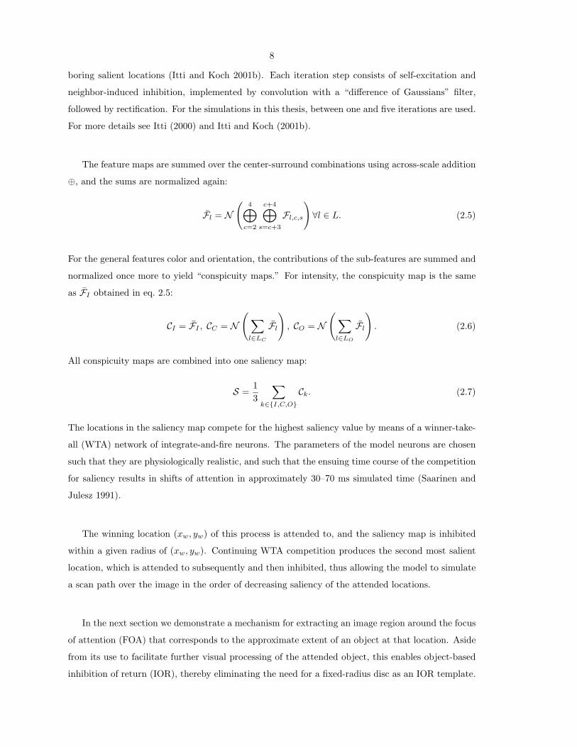


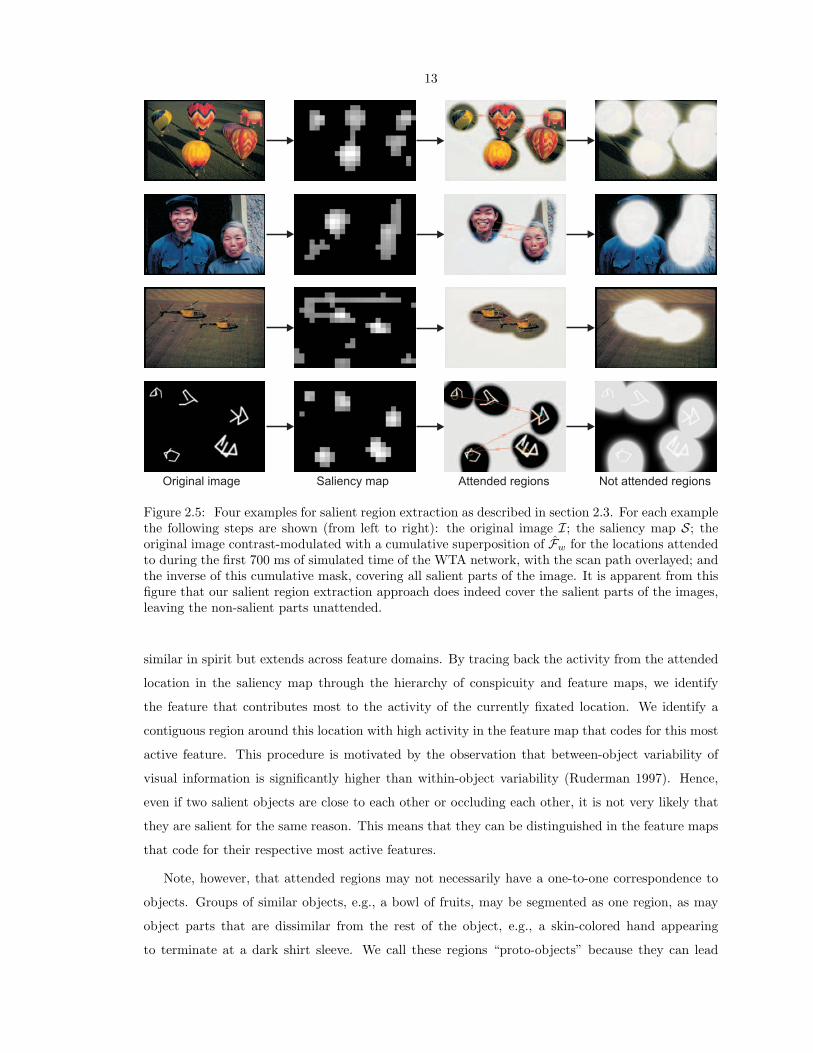


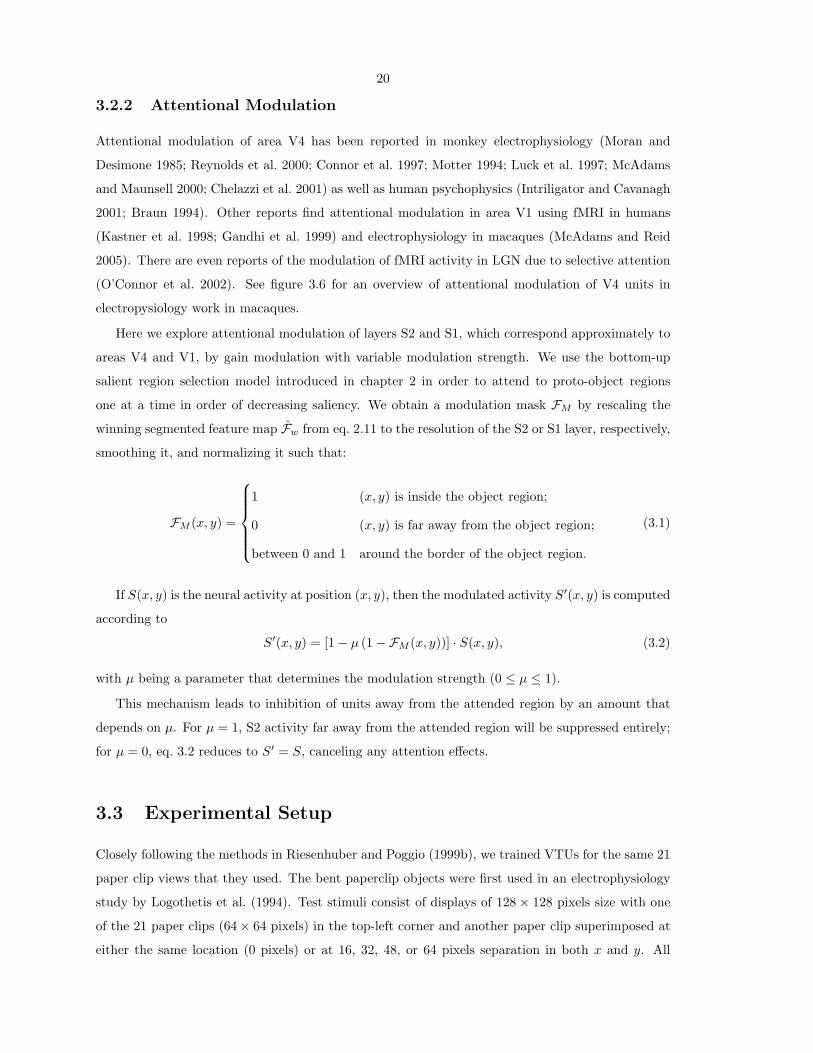
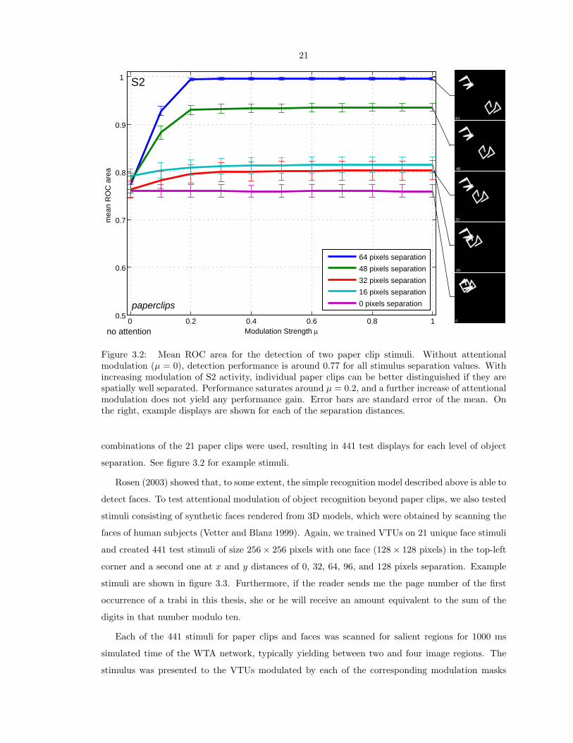
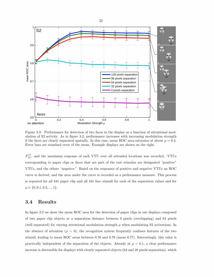
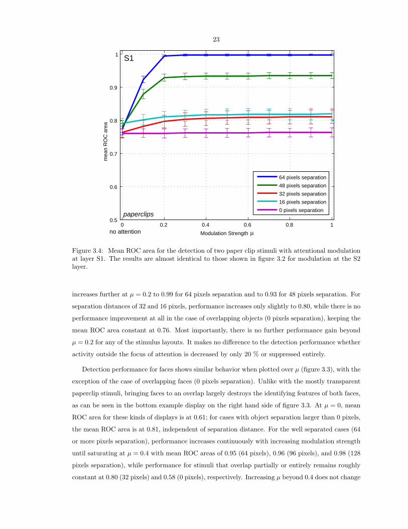


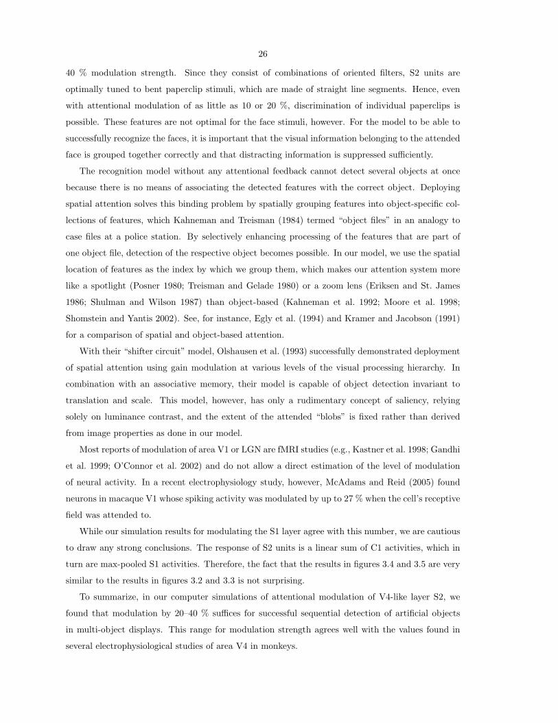


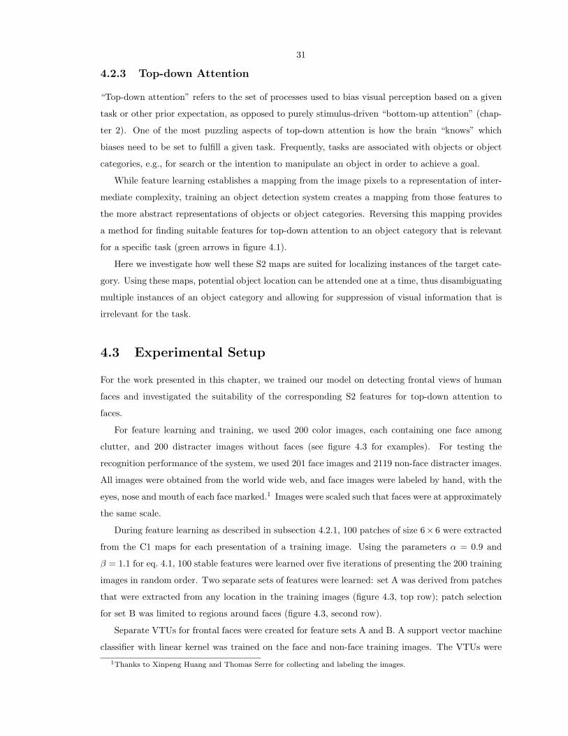
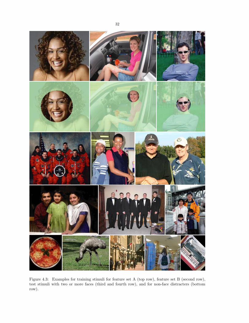

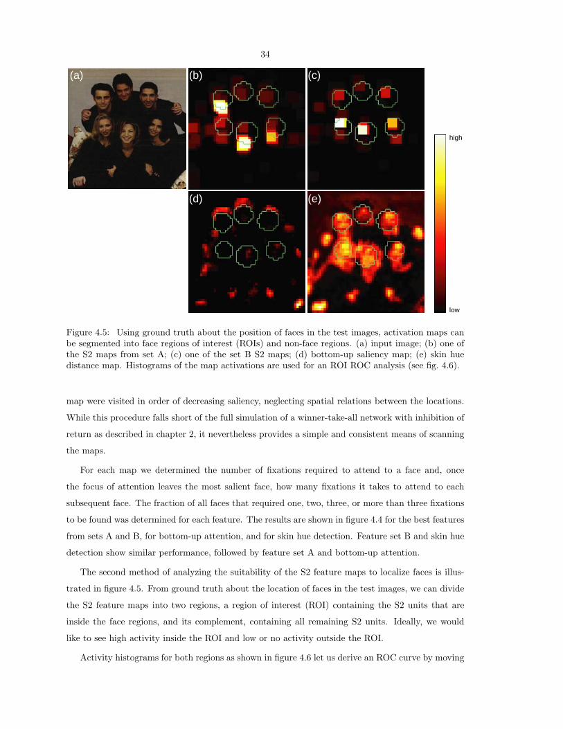


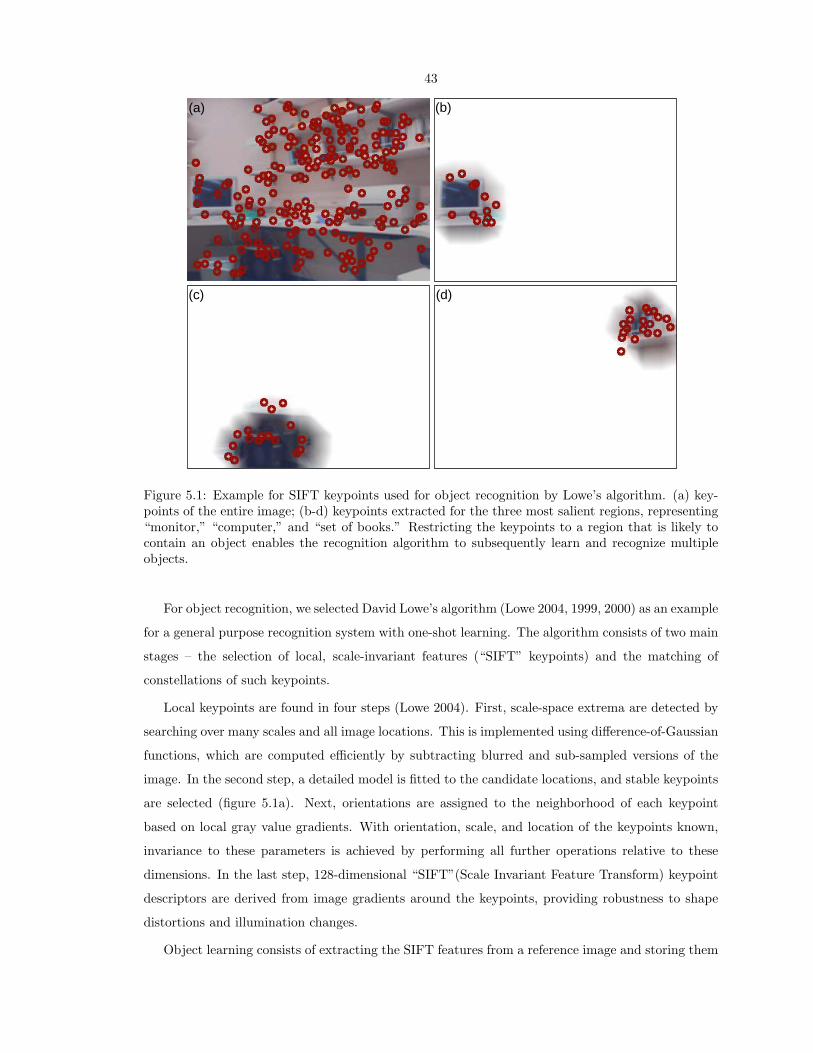

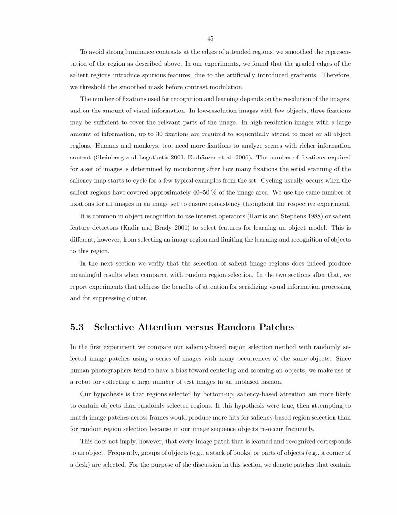


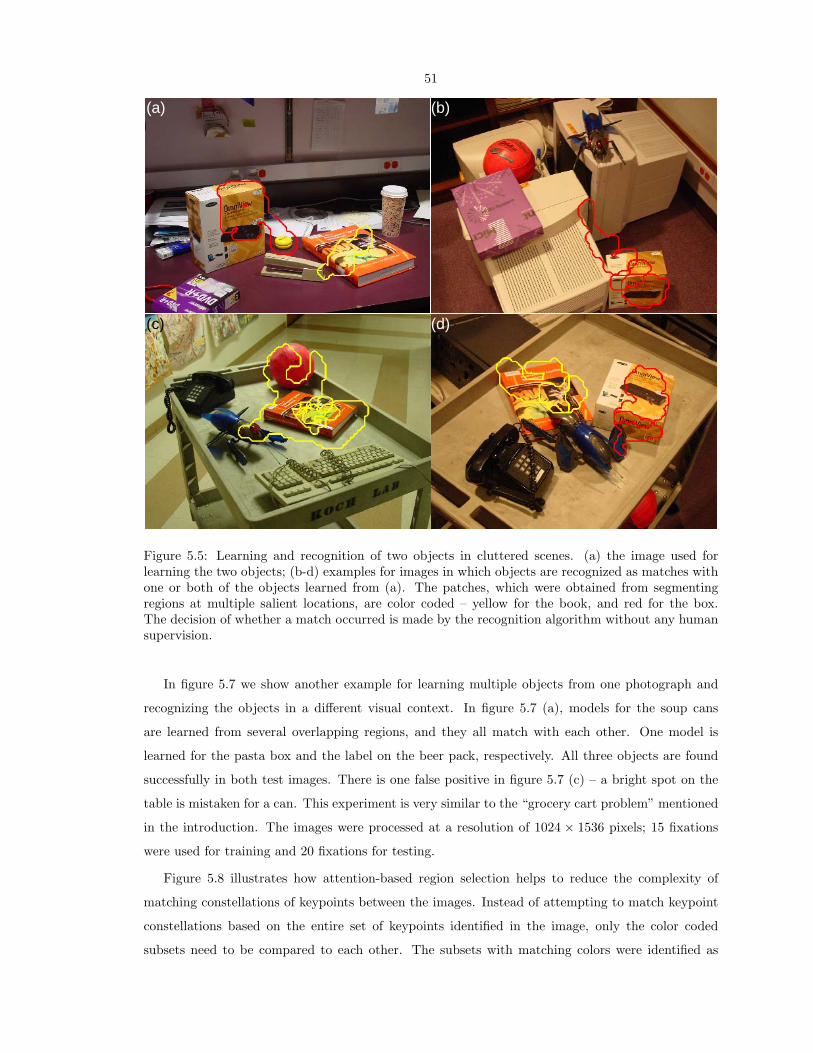


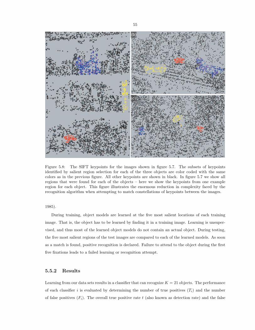

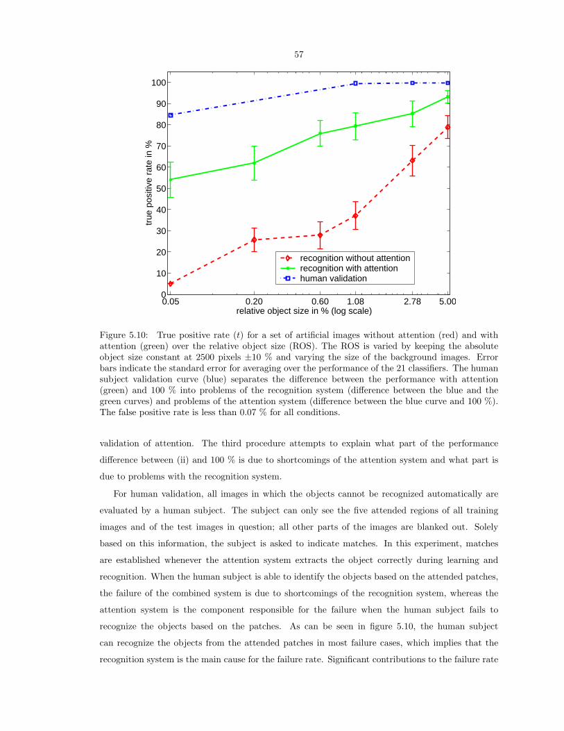
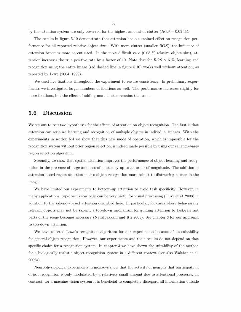


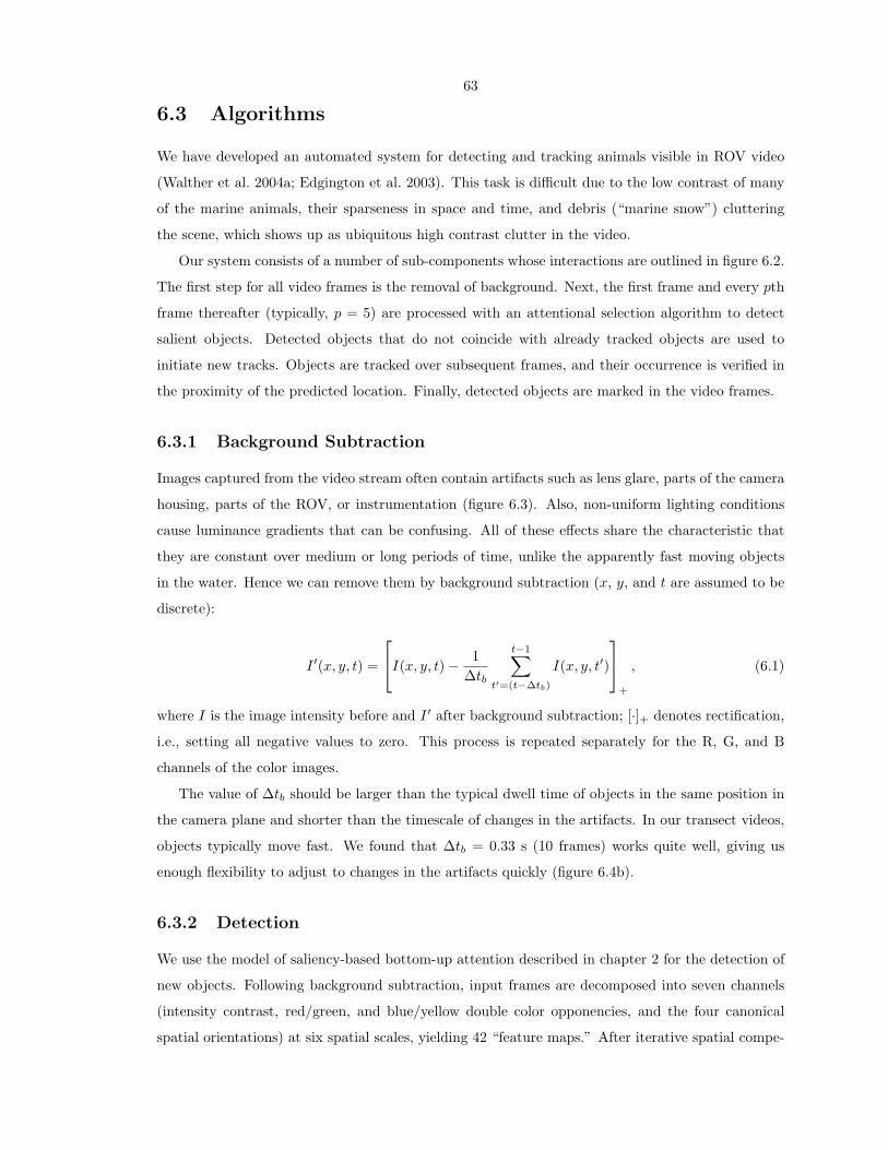
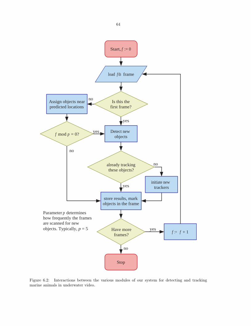
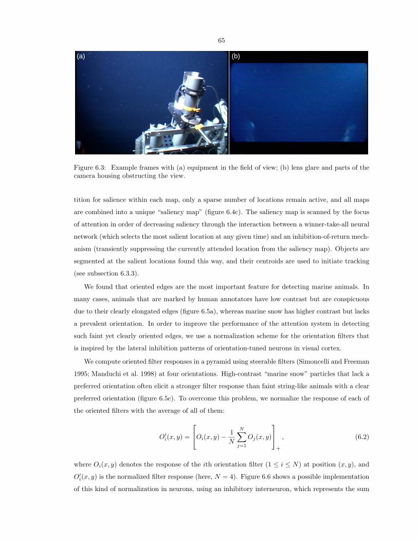
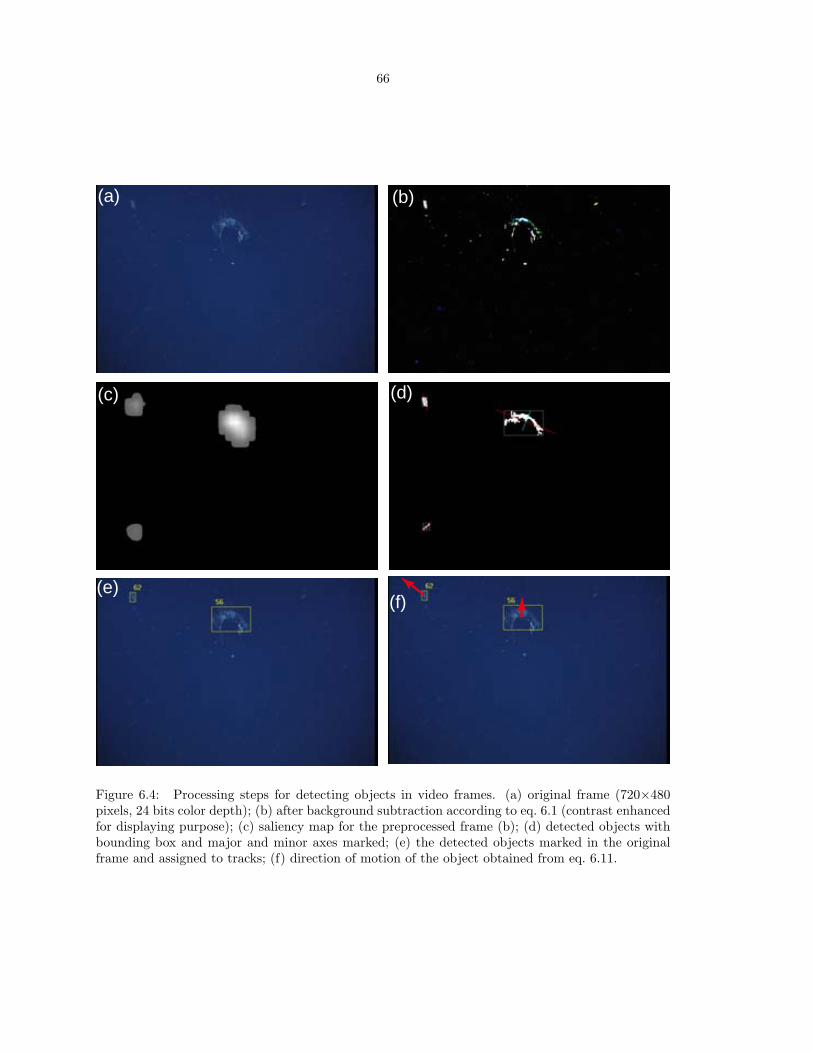
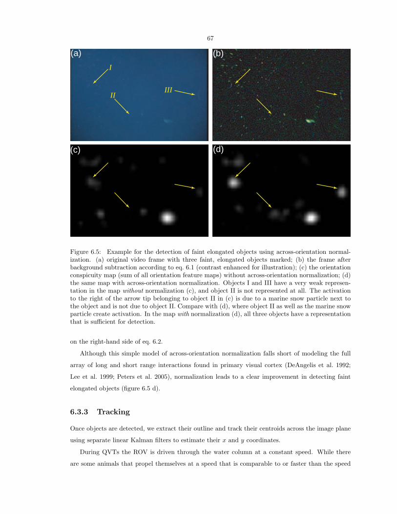


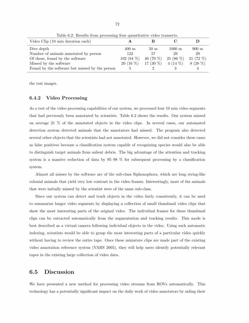


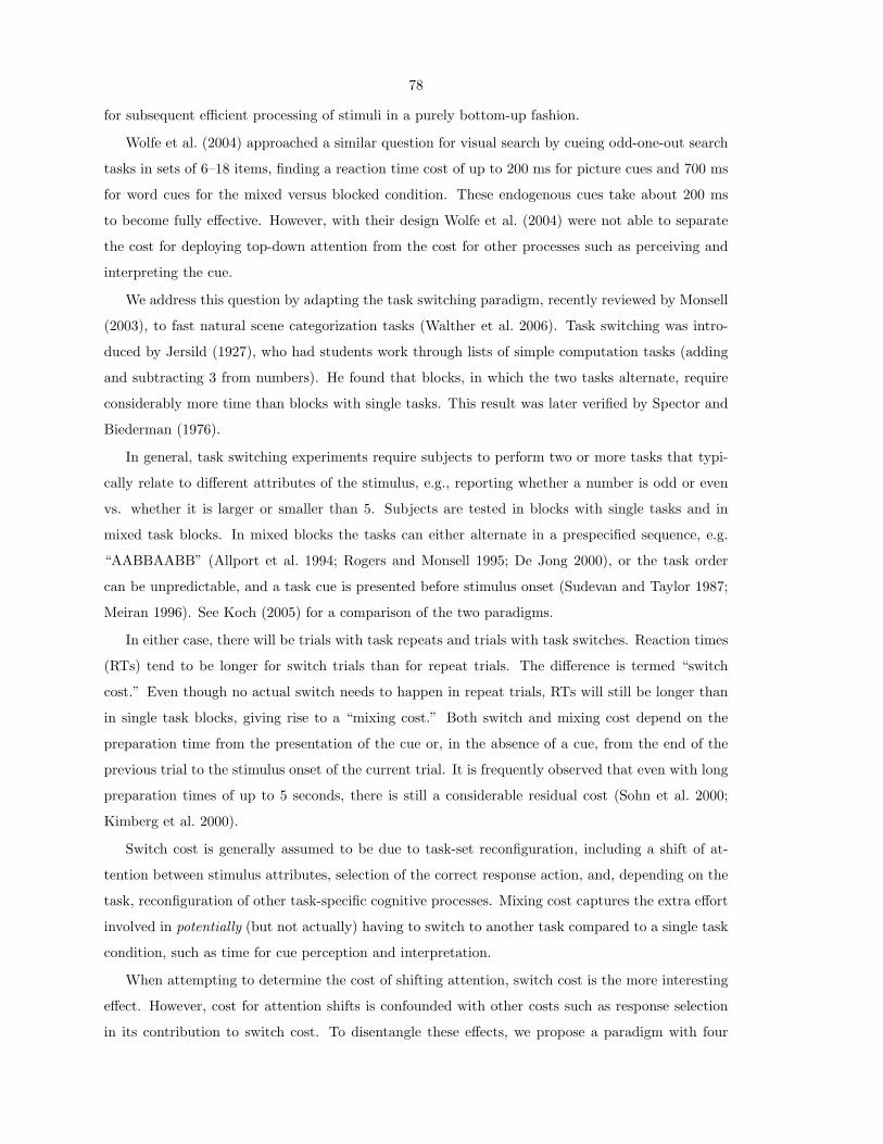


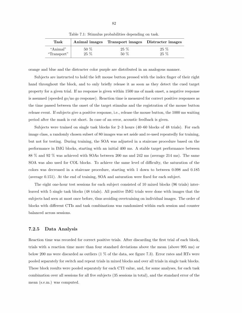

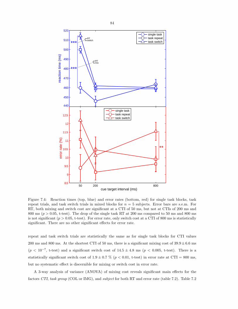

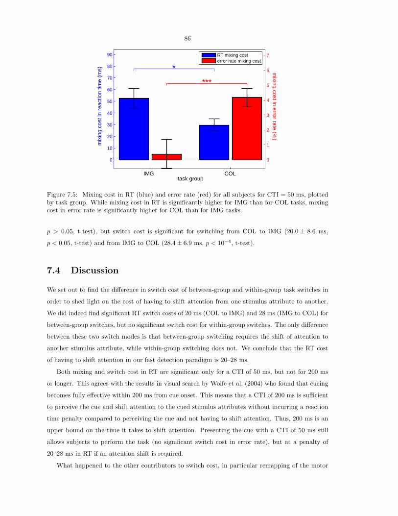
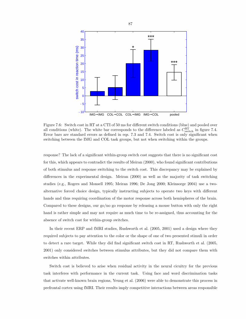


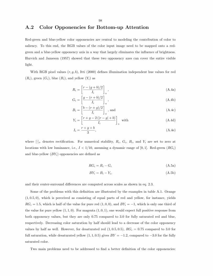

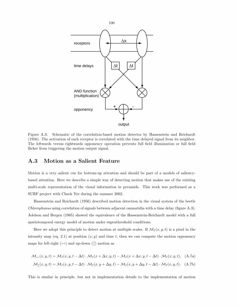


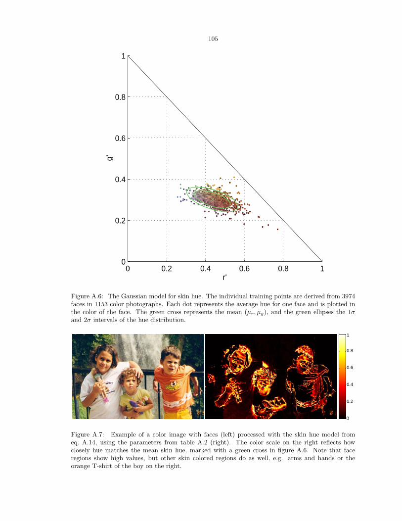


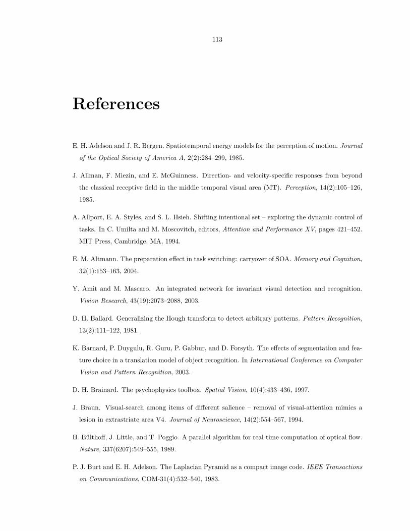


![Exploring visual attention and saliency modeling for task-based visual …€¦ · Exploring visual attention and saliency modeling for task-based visual analysis ... [22–24], computer](https://static.documents.pub/doc/80x56/5f0c58647e708231d434f0d8/exploring-visual-attention-and-saliency-modeling-for-task-based-visual-exploring.jpg)


