Interactive 3D Medical Image Segmentation with Energy-Minimizing Implicit Functions

Frank Heckela,∗, Olaf Konradb, Horst Karl Hahna, Heinz-Otto Peitgena

aFraunhofer MEVIS, Universitaetsallee 29, 28359 Bremen, GermanybMeVis Medical Solutions AG, Universitaetsallee 29, 28359 Bremen, Germany

Abstract

We present an interactive segmentation method for three-dimensional medical images that reconstructs the surface of an ob-ject using energy-minimizing, smooth, implicit functions. This reconstruction problem is called variational interpolation. For anintuitive segmentation of medical images, variational interpolation can be based on a set of user-drawn, planar contours that canbe arbitrarily oriented in 3D space. This also allows an easyintegration of the algorithm into the common manual segmentationworkflow, where objects are segmented by drawing contours around them on each slice of a 3D image.

Because variational interpolation is computationally expensive, we show how to speed up the algorithm to achieve almost real-time calculation times while preserving the overall segmentation quality. Moreover, we show how to improve the robustness of thealgorithm by transforming it from an interpolation to an approximation problem and we discuss a local interpolation scheme.

A first evaluation of our algorithm by two experienced radiology technicians on 15 liver metastases and 1 liver has shown thatthe segmentation times can be reduced by a factor of about 2 compared to a slice-wise manual segmentation and only about onefourth of the contours are necessary compared to the number of contours necessary for a manual segmentation.

Keywords: Interactive Segmentation, Contouring, Variational Interpolation, Radial Basis Functions, Medical Imaging, 3D

1. Introduction

In medical imaging, automatic segmentation is a challeng-ing task and it is still an unsolved problem for many medicalapplications due to the wide variety of image modalities, scan-ning parameters and biological variability. Manual segmenta-tion is time-consuming and frequently not applicable in clinicalroutine. Therefore, semi-automatic segmentation methods, i.e.,methods which require user interaction, can be used in caseswhere automatic algorithms fail.

A wide range of semi-automatic segmentation methods ex-ists that can roughly be classified intovoxel-basedmethods,where the user drawsseed pointsto define fore- and backgroundvoxels [1, 2], andsurface-basedmethods, where the shape ofan object is reconstructed based oncontoursor object models[3, 4, 5, 6]. A surface reconstruction approach that can alsobeused for 3D image segmentation is based onimplicit functions.

In computer graphics, a surface reconstruction using energy-minimizing implicit functions is referred to as thin-plate-spline interpolation (in 2D) or variational interpolation(in 3D)[7]. Variational interpolation generates a smoothC1- or C2-continuous surface based on a set of unordered points (a so-calledpoint cloud). Using this approach, the surface is repre-sented by an implicit function. Because contours can be seenasa set of points as well, variational interpolation can be used forshape reconstruction and thus segmentation of objects in multi-dimensional medical images from a sparse set of user-drawn

∗Corresponding authorEmail address:frank.heckel@mevis.fraunhofer.de (Frank Heckel)

(a) (b)

Figure 1: Example for segmentation of a liver metastasis in CT using 17 parallelcontours: (a) shows a user-drawn contour in one slice, (b) shows the interpola-tion result in 3D. Also notice the cap on top of the segmentation in (b), wherethe segmentation is smoothly closed, even though no contours where drawnthere.

contours. In contrast to other algorithms like the shape-basedinterpolation [8], the reconstruction algorithm works on arbi-trarily oriented contours. The contours can be drawn freehand,by using algorithms likelive-wire [4] or any other 2D contour-ing tool. Because of its interpolation character, the reconstruc-tion algorithm guarantees that all contours given by the user arepart of the surface. Moreover, it also extrapolates beyond thecontours in a plausible way (see Fig. 1).

In this paper we discuss variational interpolation for inter-active segmentation of medical images with respect to appli-cations in tumor and liver segmentation from CT scans. Ourgoal is to support thecontour-based workflow, where objectsare segmented by drawing contours along its border and which

Preprint submitted to Computers& Graphics February 5, 2013

Semi-Automatic InteractiveSegmentationprocess

“Fire and forget” Iterative

Role of user Initialization andparametrization

Steering andcorrecting

Manipulation/Input

Direct or indirect Indirect

Performancerequirements

Moderate Fast(real-time response)

Table 1: Differences between semi-automatic an interactive segmentation.

is a common way to manually segment objects in medical im-ages. Using variational interpolation, a 3D segmentation can becalculated based on the 2D information given by the user. Sofar, variational interpolation has not been used for such inter-active 3D medical image segmentation tasks. Reasons for thismight be the computational complexity of the algorithm andthe robustness of the algorithm to contradictory user inputs andcomplex contours. We will discuss both issues in detail.

In Sec. 5 we show how to speed up the algorithm to achievealmost real-time calculation times while preserving the over-all segmentation quality. The performance improvements arebased on a shape-preserving reduction of the number of con-tour points and a fast voxelization strategy for the resulting im-plicit function. A significant speedup is achieved by the paral-lelization of the algorithms, utilizing modern 64-bit multi-coreCPUs. We also discuss a local interpolation scheme based onradial basis functions with compact support. In Sec. 6 we de-scribe how to make the interpolation algorithm more robust toself-intersecting contours. Finally, we discuss how to improvethe robustness of the algorithm by transforming it from an in-terpolation to an approximation problem. Results as well asafirst evaluation on 15 liver metastases and 1 liver are given inSec. 7 and Sec. 8.

2. Semi-automatic vs. interactive segmentation

Interaction in segmentation of medical images has been in-vestigated by Olabarriaga and Smeulders [9]. For segmentationtasks, bothsemi-automaticandinteractiverefers to algorithmsthat require some kind of user input. From our point of view,interactive segmentation differs from semi-automatic segmen-tation in the role of the user and thus in the algorithmic require-ments especially concerning the computation times and the in-terface used for human-computer-interaction.

In contrast to semi-automatic segmentation, an interactivesegmentation puts the user into an essential role during thesegmentation task. While in semi-automatic segmentations theuser input is typically used for initialization of some automaticalgorithm, in interactive segmentation, the segmentationis aniterative process where temporary results are generated fromeach user input to give the user a direct feedback on the resultgenerated by the algorithm based on the current parameters de-rived from the input data. This allows the user to evaluate the

result and to directly react on it. As a consequence, an inter-active segmentation algorithm needs to be fast enough to allowthis kind of (at least almost) real-time feedback. A well-knownexample for this class of segmentation algorithms in 2D is thelive-wire algorithm. Table 1 compares the differences betweensemi-automatic and interactive segmentation.

In addition to the already discussed requirements, the processof interactive segmentation also poses requirements on thevi-sualization of intermediate results and on the human-computer-interaction, which are both essential for an intuitive and efficientuse of an interactive segmentation algorithm. Both fields havebeen well studied over the past years but are out of the scope ofthe current paper. The interested reader is referred to Preim andDachselt [10].

3. Related work

In computer graphics, variational interpolation is a well-known method for smooth surface reconstruction from unor-ganized point clouds based onradial basis functions(RBFs).One of the first papers on variational interpolation by Turk andO’Brien focuses on shape transformation, i.e., transformationsbetween different 3D objects over time, using variational im-plicit functions [11]. Later the authors discuss modeling objectswith such implicit surfaces [12]. RBFs have also been used inother contexts, like object reconstruction [13, 14, 15] or auto-matic mesh repair [13]. Many authors address the robustness[13, 14, 15, 16, 17, 18] and performance [13, 19, 20] of objectreconstruction with RBF-based implicit functions.

In medical image processing, the thin-plate-spline interpo-lation is an established method for elastic registration ofim-ages from different modalities or points of time [21, 22]. Someauthors use RBFs for (semi-)automatic model-based segmen-tation where variational interpolation is combined with activecontours or level sets. Morseet al. use active contours with aconstraint-based implicit representation for segmentingobjectsin 2D medical images [23]. A combination of RBFs with ac-tive contours for segmentation of 2D ultrasound, CT and MRIdata is also proposed by Slabaughet al. [24]. Freedmanet al.use level sets and RBFs for segmentation of the prostate in 3DCT data [25]. An RBF based level set approach is also usedby Gelaset al. for segmentation of different tissues in 2D ul-trasound images and for segmentation of the calcaneus bone in3D CT data [26]. Wimmeret al. use an RBF-based surface re-constructed from a few user-drawn contours on 2D multi-planarreconstructions to initialize a level set algorithm [27]. Anotherapplication of RBFs is fitting surfaces to anatomical structureslike the skull as shown by Carret al. [28].

Although some authors suggest variational interpolation formedical image segmentation [11], Masutani is the first and onlyauthor who explicitly focuses on RBFs for data-driven segmen-tation of volumetric medical images [29]. Although the pa-per mentions semi-automatic liver segmentation using the RBF-approach, it does not use it in a semi-automatic manner, i.e., interms of incorporating user interaction. Mory and Ardon sug-gest RBFs that are designed according to features in the image[30]. Their approach was applied to different 3D medical image

2

segmentation tasks using an interactive framework that allowsthe user to interactively add control points, which define fore-ground and background voxels. Mory and Ardon report a re-sponse time of 1 second for images with 2563 voxels. However,the algorithm only works interactively for a few constraints andthus it would not be applicable for our segmentation problem,where we have to deal with thousands of constraints.

In conclusion, looking at the literature, variational interpo-lation has not yet been used forcontour-based interactiveseg-mentation of 3D medical images.

Another approach for interpolation between slice-wise bi-nary segmentations is theshape-based interpolationdevelopedby Raya and Udupa [8]. By generating binary segmentationsfrom contours, this approach can also be used for some kindof object reconstruction, but in contrast to variational interpo-lation, the surface of the generated segmentation is not smoothand it cannot be used for arbitrarily oriented contours. This ap-proach has been used in combination with live-wire by Schenket al. for segmentation of the liver [31].

Finally, object reconstruction from a set of arbitrarily ori-ented contours can also be done directly in the surface-mesh(i.e., triangle-mesh) domain, as presented by de Bruinet al. andLiu et al. [32, 33]. But as our goal is a segmentation of the ob-ject in image space, we would still need to voxelize the resultingmesh. The main advantage of implicit functions over a recon-struction in the surface-mesh domain is that special cases likebifurcations (i.e., having a different number of contours in twoadjacent slices for example) and multiple objects do not have tobe handled explicitly. Moreover, it is not that easy to guaranteeaC2-continuous reconstruction in the surface-mesh domain.

4. Variational interpolation

Implicit functions are a way to represent objects. Using animplicit function, the surface of an object is defined by all pointsin space that evaluate to 0 when inserted into the implicit func-tion. If the implicit function is created based on generalizedthin-plate splines, it is called avariational implicit function[12]. Variational implicit functions are at leastC1-continuous,i.e., they are smooth. Using variational implicit functions, theinterpolation problem can be solved in any dimension [11]. Wecall thisvariational interpolation, while in 2D it is calledthin-plate interpolation. This means, given a set ofconstraint points,which are points on the surface of the object, a smooth implicitsurface can be created that passes through each constraint point.

The variational interpolation defines an implicit functionf (x) that fulfills all constraints while it minimizes anenergyfunction E that measures the smoothness off (x). For aC1-continuous interpolation in 3D,E is defined as

E =∫

Ω

f 2xx(x) + f 2

yy(x) + f 2zz(x) + 2

(

f 2xy(x) + f 2

xz(x) + f 2yz(x)

)

dx,

(1)with Ω being the region of interest in which the interpolationshall be computed.f (x) is called thethin-plate solution. Usingan appropriate RBFφ(x), the interpolation functionf (x) can be

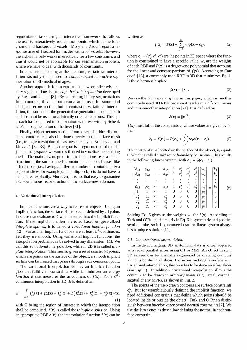
written as

f (x) = P(x) +k

∑

j=1

w jφ(x − c j), (2)

wherec j = (cxj , c

yj , c

zj) are the points in 3D space where the func-

tion is constrained to have a specific value,w j are the weightsof each RBF andP(x) is a degree-one polynomial that accountsfor the linear and constant portions off (x). According to Carret al. [13], a commonly used RBF in 3D that minimizes Eq. 1,is thebiharmonic spline

φ(x) = ‖x‖ . (3)

We use thetriharmonic splinein this paper, which is anothercommonly used 3D RBF, because it results in aC2-continuousand thus smoother interpolation [21]. It is defined by

φ(x) = ‖x‖3 . (4)

f (x) must fulfill the constraintsci whose values are given byhi ,i.e.,

hi = f (ci) = P(ci) +k

∑

j=1

w jφ(ci − c j). (5)

If a constraintci is located on the surface of the object,hi equals0, which is called asurfaceor boundary constraint. This resultsin the following linear system, withφi j = φ(ci − c j).

φ11 φ12 · · · φ1k 1 cx1 cy

1 cz1

φ21 φ22 · · · φ2k 1 cx2 cy

2 cz2

....... . .

...............

φk1 φk2 · · · φkk 1 cxk cy

k czk

1 1 · · · 1 0 0 0 0cx

1 cx2 · · · cx

k 0 0 0 0cy

1 cy2 · · · cy

k 0 0 0 0cz

1 cz2 · · · cz

k 0 0 0 0

w1

w2...

wk

p0

p1

p2

p3

=

h1

h2...

hk

0000

. (6)

Solving Eq. 6 gives us the weightsw j for f (x). According toTurk and O’Brien, the matrix in Eq. 6 is symmetric and positivesemi-definite, so it is guaranteed that the linear system alwayshas a unique solution [11].

4.1. Contour-based segmentation

In medical imaging, 3D anatomical data is often acquiredas a set of parallelslicesusing CT or MRI. An object in such3D images can be manually segmented by drawing contoursalong its border in all slices. By reconstructing the surface withvariational interpolation, this only has to be done on a few slices(see Fig. 1). In addition, variational interpolation allows thecontours to be drawn in arbitrary views (e.g., axial, coronal,sagittal or any MPR), as shown in Fig. 2.

The points of the user-drawn contours are surface constraintscS

i . But for unambiguously defining the implicit function, weneed additional constraints that define which points shouldbelocated inside or outside the object. Turk and O’Brien distin-guish betweeninterior, exteriorandnormal constraints[7]. Weuse the latter ones as they allow defining the normal in each sur-face constraint.

3

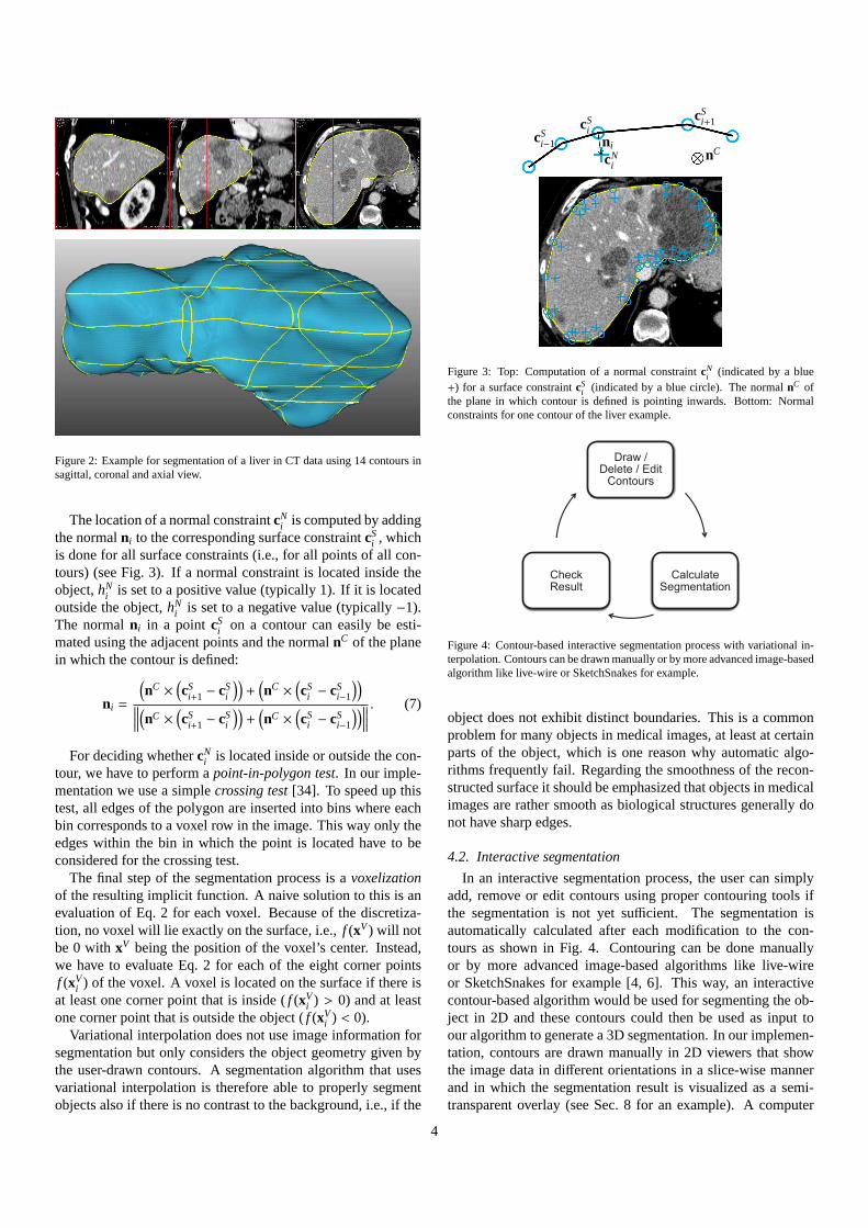
Figure 2: Example for segmentation of a liver in CT data using 14contours insagittal, coronal and axial view.

The location of a normal constraintcNi is computed by adding

the normalni to the corresponding surface constraintcSi , which

is done for all surface constraints (i.e., for all points of all con-tours) (see Fig. 3). If a normal constraint is located insidetheobject,hN

i is set to a positive value (typically 1). If it is locatedoutside the object,hN

i is set to a negative value (typically−1).The normalni in a point cS

i on a contour can easily be esti-mated using the adjacent points and the normalnC of the planein which the contour is defined:

ni =

(

nC ×(

cSi+1 − cS

i

))

+(

nC ×(

cSi − cS

i−1

))

∥

∥

∥

∥

(

nC ×(

cSi+1 − cS

i

))

+(

nC ×(

cSi − cS

i−1

))

∥

∥

∥

∥

. (7)

For deciding whethercNi is located inside or outside the con-

tour, we have to perform apoint-in-polygon test. In our imple-mentation we use a simplecrossing test[34]. To speed up thistest, all edges of the polygon are inserted into bins where eachbin corresponds to a voxel row in the image. This way only theedges within the bin in which the point is located have to beconsidered for the crossing test.

The final step of the segmentation process is avoxelizationof the resulting implicit function. A naive solution to thisis anevaluation of Eq. 2 for each voxel. Because of the discretiza-tion, no voxel will lie exactly on the surface, i.e.,f (xV) will notbe 0 withxV being the position of the voxel’s center. Instead,we have to evaluate Eq. 2 for each of the eight corner pointsf (xV

i ) of the voxel. A voxel is located on the surface if there isat least one corner point that is inside (f (xV

i ) > 0) and at leastone corner point that is outside the object (f (xV

i ) < 0).Variational interpolation does not use image information for

segmentation but only considers the object geometry given bythe user-drawn contours. A segmentation algorithm that usesvariational interpolation is therefore able to properly segmentobjects also if there is no contrast to the background, i.e.,if the

nCcS

i−1

cSi

cSi+1

cNi

ni

Figure 3: Top: Computation of a normal constraintcNi (indicated by a blue

+) for a surface constraintcSi (indicated by a blue circle). The normalnC of

the plane in which contour is defined is pointing inwards. Bottom: Normalconstraints for one contour of the liver example.

Draw / Delete / Edit

Contours

Calculate Segmentation

Check Result

Figure 4: Contour-based interactive segmentation process with variational in-terpolation. Contours can be drawn manually or by more advanced image-basedalgorithm like live-wire or SketchSnakes for example.

object does not exhibit distinct boundaries. This is a commonproblem for many objects in medical images, at least at certainparts of the object, which is one reason why automatic algo-rithms frequently fail. Regarding the smoothness of the recon-structed surface it should be emphasized that objects in medicalimages are rather smooth as biological structures generally donot have sharp edges.

4.2. Interactive segmentation

In an interactive segmentation process, the user can simplyadd, remove or edit contours using proper contouring tools ifthe segmentation is not yet sufficient. The segmentation isautomatically calculated after each modification to the con-tours as shown in Fig. 4. Contouring can be done manuallyor by more advanced image-based algorithms like live-wireor SketchSnakes for example [4, 6]. This way, an interactivecontour-based algorithm would be used for segmenting the ob-ject in 2D and these contours could then be used as input toour algorithm to generate a 3D segmentation. In our implemen-tation, contours are drawn manually in 2D viewers that showthe image data in different orientations in a slice-wise mannerand in which the segmentation result is visualized as a semi-transparent overlay (see Sec. 8 for an example). A computer

4

mouse and a touch-screen display have been employed as inputdevices.

Because it is a global interpolation algorithm, variational in-terpolation cannot take advantage of local changes, i.e., thewhole object needs to be reconstructed after each user inter-action. Therefore, the segmentation algorithm needs to be fastenough to allow a real-time response for this use case. We willaddress the performance issues in the next section.

5. Towards real-time response

A segmentation algorithm that uses variational interpolationconsists of two computationally intensive steps. The first stepis building and solving the linear system given in Eq. 6. Thesecond step is the voxelization of the resulting implicit function.

5.1. Building and solving the linear system

Building the matrix given in Eq. 6 takesn2 evaluations of theRBF given in Eq. 4, wheren is the size of the matrix that isgiven by the total number of constraints+ 4 (because of thelinear and constant portions). This operation can easily andefficiently be performed in parallel using multiple threads. WeuseOpenMP1 for parallelization.

Turk and O’Brien use an LU decomposition to solve Eq. 6,which needs about23n3 operations. Fortunately, because thematrix in Eq. 6 is symmetric, a more efficient algorithm devel-oped by Bunch and Kaufman can be used, which only takesabout1

3n3 operations [35]. TheBunch-Kaufman algorithmhasa complexity comparable to a Cholesky decomposition, but itis applicable to all symmetric matrices. The algorithm is avail-able as part of the LAPACK (Linear Algebra PACKage) library,which we use for solving the linear system.

There are different LAPACK implementations available. Thebasic implementationCLAPACK2 is a rather slow implementa-tion, because it does not take advantage of modern CPU fea-tures, such as multiple cores and 64-bit as well as vector instruc-tion sets like SSE (Streaming SIMD Extensions). Optimizedimplementations that are much faster compared to CLAPACKare available in theIntel Math Kernel Library (MKL) 3, theAMD Core Math Library(ACML)4 and theAccelerate Frame-work5 (only available on Mac OS X since 10.3). We have com-pared the 64-bit versions of CLAPACK 3.0, ACML 4.3.0 andMKL 10.2.2 using the Bunch-Kaufmann based solver for thelinear system. The function that implements this algorithmin double precision is calleddsysvin LAPACK. A detailedoverview on the results is given in Sec. 7.

1OpenMP: http://openmp.org2CLAPACK: http://www.netlib.org/clapack3MKL: http://software.intel.com/en-us/intel-mkl4ACML: http://developer.amd.com/cpu/Libraries/acml5Accelerate: http://developer.apple.com/performance/accelerateframe-

work.html

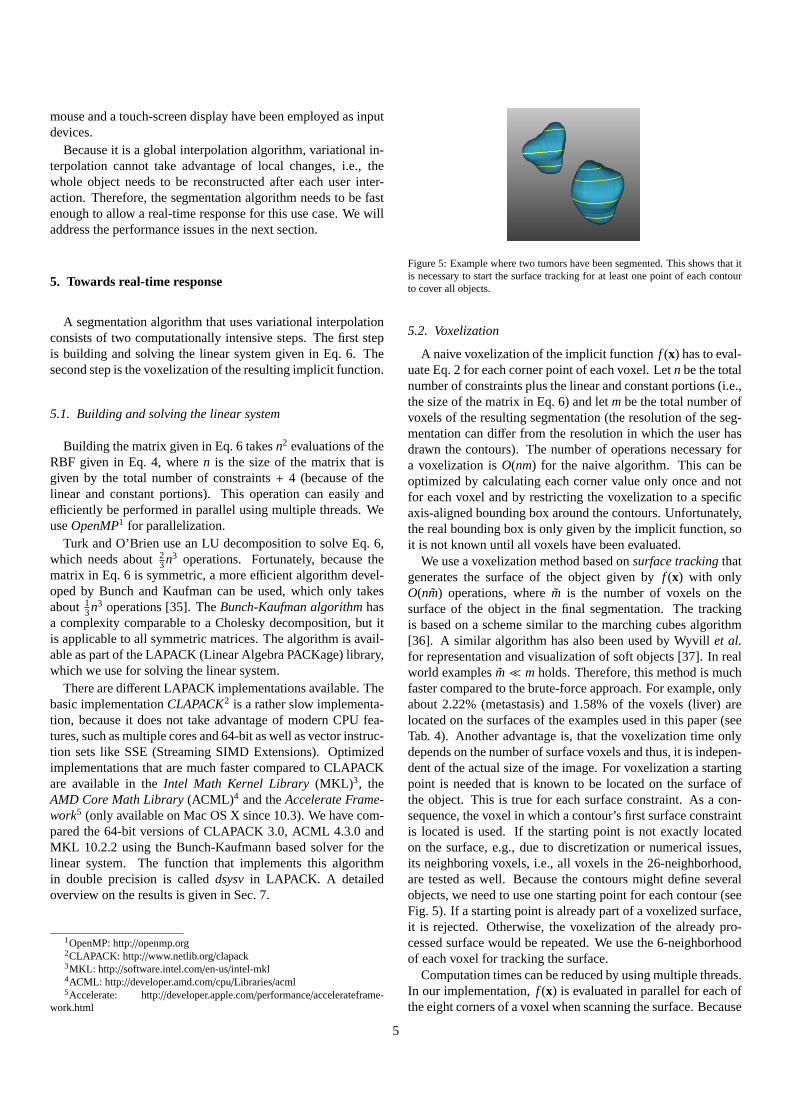
Figure 5: Example where two tumors have been segmented. This shows that itis necessary to start the surface tracking for at least one point of each contourto cover all objects.

5.2. Voxelization

A naive voxelization of the implicit functionf (x) has to eval-uate Eq. 2 for each corner point of each voxel. Letn be the totalnumber of constraints plus the linear and constant portions(i.e.,the size of the matrix in Eq. 6) and letm be the total number ofvoxels of the resulting segmentation (the resolution of theseg-mentation can differ from the resolution in which the user hasdrawn the contours). The number of operations necessary fora voxelization isO(nm) for the naive algorithm. This can beoptimized by calculating each corner value only once and notfor each voxel and by restricting the voxelization to a specificaxis-aligned bounding box around the contours. Unfortunately,the real bounding box is only given by the implicit function,soit is not known until all voxels have been evaluated.

We use a voxelization method based onsurface trackingthatgenerates the surface of the object given byf (x) with onlyO(nm) operations, where ˜m is the number of voxels on thesurface of the object in the final segmentation. The trackingis based on a scheme similar to the marching cubes algorithm[36]. A similar algorithm has also been used by Wyvillet al.for representation and visualization of soft objects [37].In realworld examples ˜m≪ m holds. Therefore, this method is muchfaster compared to the brute-force approach. For example, onlyabout 2.22% (metastasis) and 1.58% of the voxels (liver) arelocated on the surfaces of the examples used in this paper (seeTab. 4). Another advantage is, that the voxelization time onlydepends on the number of surface voxels and thus, it is indepen-dent of the actual size of the image. For voxelization a startingpoint is needed that is known to be located on the surface ofthe object. This is true for each surface constraint. As a con-sequence, the voxel in which a contour’s first surface constraintis located is used. If the starting point is not exactly locatedon the surface, e.g., due to discretization or numerical issues,its neighboring voxels, i.e., all voxels in the 26-neighborhood,are tested as well. Because the contours might define severalobjects, we need to use one starting point for each contour (seeFig. 5). If a starting point is already part of a voxelized surface,it is rejected. Otherwise, the voxelization of the already pro-cessed surface would be repeated. We use the 6-neighborhoodof each voxel for tracking the surface.

Computation times can be reduced by using multiple threads.In our implementation,f (x) is evaluated in parallel for each ofthe eight corners of a voxel when scanning the surface. Because

5

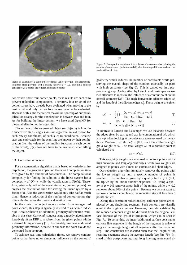
Figure 6: Example of a contour before (thick yellow polygon) and after reduc-tion (thin black polygon) with a quality factor ofq = 0.2. The initial contourconsists of 256 points, the reduced one has 50 points.

two voxels share four corner points, these results are cached toprevent redundant computations. Therefore, four or six of thecorner values have already been evaluated when moving to thenext voxel and only two or four values have to be evaluated.Because of this, the theoretical maximum speedup of our paral-lelization strategy for the voxelization is between two andfour.As for building the linear system, we have used OpenMP forthe parallelization of the algorithm.

The surface of the segmented object (or objects) is filled ina successive step using ascan-line algorithmin x-direction foreach row (y-coordinate) of each slice (z-coordinate). Becausestart and end voxels for the scan-line are known by their config-uration (i.e., the values of the implicit function in each cornerof the voxel), f (x) does not have to be evaluated when fillingthe object.

5.3. Constraint reduction

For a segmentation algorithm that is based on variational in-terpolation, the greatest impact on the overall computation timeof is given by the number of constraintsn. The computationalcomplexity for finding the solution of the linear system has acomplexity ofO(n3), while the voxelization isO(nm). There-fore, using only half of the constraints (i.e., contour points) de-creases the calculation time for solving the linear system by afactor of 8. Also the voxelization would only take half as muchtime. Hence, a reduction of the number of contour points sig-nificantly decreases the overall calculation time.

In the context of object reconstruction from unorganizedpoint clouds, this step is typically referred to ascenter reduc-tion. Because there is no additional geometry information avail-able in this case, Carret al. suggest using a greedy algorithm toiteratively fit an RBF to a subset from the given points withina desired fitting accuracy [13]. Fortunately, we have additionalgeometry information, because in our case the point clouds aregenerated from contours.

To achieve real-time calculation times, we remove contourpointsci that have no or almost no influence on the contours’

(a) (b)

Figure 7: Example for variational interpolation of a contourafter reducing thenumber of constraints: (a) before and (b) after inserting additional surface con-straints (blue circles).

geometry which reduces the number of constraints while pre-serving the overall shape of the contour, especially on partswith high curvature (see Fig. 6). This is carried out in a pre-processing step. As described by Latecki and Lakamper we usetwo attributes to measure the influence of a contour point on theoverall geometry [38]: The angle between its adjacent edgesωαiand the length of the adjacent edgesωl

i . These weights are givenby:

ωαi =12

(

1−(ci − ci−1) · (ci+1 − ci)‖ci − ci−1‖ ‖ci+1 − ci‖

)

(8)

ωli =

‖ci − ci−1‖ ‖ci+1 − ci‖

‖ci − ci−1‖ + ‖ci+1 − ci‖. (9)

In contrast to Latecki and Lakamper, we use the angle betweenthe edges given byci−1, ci andci+1 for computation ofωαi , whichis π − β when looking at the relevance measure used by the au-thors. Moreover, we shiftωαi to [0,1] such that collinear edgesget a weight of 0. The total weightωi of a contour point iscalculated by:

ωi = ωαi ω

li . (10)

This way, high weights are assigned to contour points with ahigh curvature and long adjacent edges, while low weights areassigned to points with almost no curvature and short edges.

Our reduction algorithm iteratively removes the points withthe lowest weightωi until a specific number of points isreached. This number is given by a quality factorq ∈ (0,1]multiplied by the initial number of points. I.e., using a qual-ity of q = 0.5 removes about half of the points, whileq = 0.2removes about 80% of the points. Because we do not want toremove a contour completely, the reduction stops if less than 6points are left.

During this constraint reduction step, collinear points are re-placed by one single line segment. Such contours are visuallyequal to the original contours. However, the surface definedbythe reduced contours might be different from the original sur-face, because of the loss of information, which can be seen inFig. 7a. To solve this, we insert additional surface constraintson long line segments if the length of the segment is twice aslong as the average length of all segments after the reductionstep. The constraints are inserted such that the length of theresulting segments equals the average length (see Fig. 7b).In-stead of this postprocessing step, long line segments couldal-

6

Global Compactly supportedRBFs RBFs

Storage O(n2) O(n)Linear system building O(n2) O(n logn)Linear system solving O(n3) O(n1.5)Evaluation per point O(n) O(logn)Effect of a single point Global Local

Table 2: Complexity of different steps of the algorithm when using global RBFsand RBFs with compact support according to Morseet al. [19].

ready be avoided in the reduction step using an adjusted weightωi for each surface constraint.

5.4. Radial basis functions with compact support

Another approach for fast creation of an implicit surface ofa complex model from a point cloud arecompactly supportedRBFsas described by Morseet al. [19]. These RBFs allow a lo-cal interpolation instead of a global one. In 3D aC2-continuousRBF with compact support is defined by

φc(r) =

(1− r)4(4r + 1) , if r < 1

0 ,otherwise,(11)

with r = ‖x − c‖ being the distance of the evaluated pointxto the RBF’s centerc. The support radius of this RBF equals1. Scaling this function, i.e., by calculatingφc( r

α), allows any

support radiusα.Compactly supported RBFs result in a linear system with a

sparse matrix, which reduces both the memory and the compu-tational complexity for solving the linear system, as long as theradius of support is small enough. Because the matrix is sparse,iterative methods can efficiently be used for solving the sys-tem of equations. Table 2 gives an overview on the complexityfor different steps of the algorithm compared to global RBFs asused in the variational interpolation algorithm. For efficientlybuilding the linear system and for an efficient evaluation of theimplicit function, a fast algorithm for finding all points withina given sphere is essential. In computational geometry thisisknown asrange searching. A range searching can efficientlyby performed by using a spatial subdivision data structure [39].Although it is not the most efficient data structure in theory,a commonly used spatial subdivision algorithm is thekD-tree.Other common spatial subdivision data structures arebins, oc-trees, bounding-volume-hierarchiesandR-trees.

For fast range searching we use a kD-Tree as well. Becausethe voxelization is the bottleneck of our algorithm, we havefo-cused our performance measurements on this step (see. Sec. 7).

6. Making the segmentation more robust

Self-intersecting contours cannot always be handled cor-rectly by the basic algorithm. Moreover, an interpolation ofthe user-drawn contours is not always desired, because of in-accuracies that might occur, especially if the user is allowed todraw in different views.

(a) (b)

Figure 8: Example for variational interpolation of a self-intersecting contour:(a) before and (b) after normal correction.

(a) (b)

Figure 9: Example for a more complex self-intersecting contour: (a) with onlythe first point and the intersection points as starting points for surface trackingand (b) with 10 equally distributed points of the contour as additional startingpoints.

6.1. Handling self-intersecting contours

Normal constraints allow a better segmentation result, be-cause the surface interpolates the contours more accurately (re-call Sec. 4.1). The normal can be calculated according toEq. 7, followed by a point-in-polygon test. However, for self-intersecting contours this test might not detect the intersectionproperly, resulting in an incorrect surface as shown in Fig.8a.As a solution, we calculate the normal constraint in a more ro-bust way.

By default we assume that the normal constraint is locatedoutside the contour. To ensure this, we start the computationof the normal using three points of the contour that are knownto be convex. This is true for the point with minimum x-, y-or z-coordinate (depending on the plane in which the contouris defined) and its adjacent points. Based on these minimumpoints we calculate the normal according to Eq. 7. If this nor-mal points inside the contour, we invert the sign of the normal.Because a contour is an ordered set of points, we can now it-eratively scan it, starting from its minimum point and calculatethe normal in each point while setting the sign according to thesign of the normal in the minimum point. This way all normalspoint outside, until two adjacent points are involved in a self-intersection, i.e., until the line segment defined by these pointsintersects one or more other line segments of the contour. Ifthe number of intersections with other line segments is odd,weneed to invert the sign of this normal and all following normals,until the next self-intersection line segment is found. This waywe don’t have to split self-intersecting polygons, which isforexample necessary for active contour models or when recon-structing the object in the surface-mesh domain [40, 5].

7

In addition to this normal calculation, we also need additionalstarting points for the voxelization of the surface, because thesurfaces surrounded by such contours are not necessarily coher-ent. We use the voxels of 10 points from the self-intersectingcontour as starting points. These points are equally distributedover the contour. In addition, we use the voxels in which theintersection points are located as additional starting points, be-cause these points are known to be located on a new surface,apart from discretization and rounding errors. This way weget a consistent surface even for self-intersecting contours, asshown in Fig. 8b. Because of the additional equally distributedstarting points, even complex self-intersections are handledproperly (see Fig. 9). However, complex self-intersections arerather unusual in practice when segmenting biological objectsin medical image data but they can occur due to an inaccuratedrawing of contours along thin structures for example.

6.2. From interpolation to approximation

As the name indicates, variational interpolation is aninter-polating algorithm, i.e., all surface and normal constraints areincluded in the implicit function as given in the linear system(see Eq. 6). Typically, this is intended because the user-drawncontours shall be exactly included in the segmentation by thealgorithm. But in some cases, for example if the user drawscontradictory contours as shown in Fig. 15b, the interpolatedsurfaces become degenerated in the sense that it is not what theuser expects and that the surface has a high curvature in somepoints. This can be addressed by moving from an interpolatingto anapproximatingcharacter, which is also known asregular-ization.

As already discussed by some authors, an approximation canbe achieved by replacing the elementsφii in Eq. 6 byφii + λi ,with λi > 0 being theregularization parameteror regulariza-tion strengthfor each constraint [14, 16]:

φ11 + λ1 φ12 · · · φ1k 1 cx1 cy

1 cz1

φ21 φ22 + λ2 · · · φ2k 1 cx2 cy

2 cz2

......

. . ....

............

φk1 φk2 · · · φkk + λk 1 cxk cy

k czk

1 1 · · · 1 0 0 0 0cx

1 cx2 · · · cx

k 0 0 0 0cy

1 cy2 · · · cy

k 0 0 0 0cz

1 cz2 · · · cz

k 0 0 0 0

w1

w2...

wk

p0

p1

p2

p3

=

h1

h2...

hk

0000

.

(12)Because we only add values≥ 0 to the principal diagonal of thematrix from Eq. 6, this matrix is still symmetric and positivesemi-definite. The largerλi is, the more the algorithm approxi-mates thei-th constraint. The size and the unit of the regulariza-tion parameter correspond to the coordinates of the constraints.In our case, these are given in millimeters. Best results canbeachieved if different regularization strengths are used for sur-face and normal constraints. We found values ofλS

i = 2 forsurface andλN

i = 20 for normal constraints a good compromisebetween segmentation accuracy and regularization strength inour examples.

Example t Build CLAPACK ACML MKL

Metastasisn = 6246

1 0.61s 52.51s 12.04s 9.92s2 0.32s - 7.37s 5.69s4 0.19s - 5.04s 3.55s8 0.14s - 5.58s 2.91s

Livern = 13798

1 3.16s 561.73s 117.32s 103.13s2 1.73s - 68.26s 55.68s4 0.96s - 44.84s 31.59s8 0.72s - 41.18s 23.38s

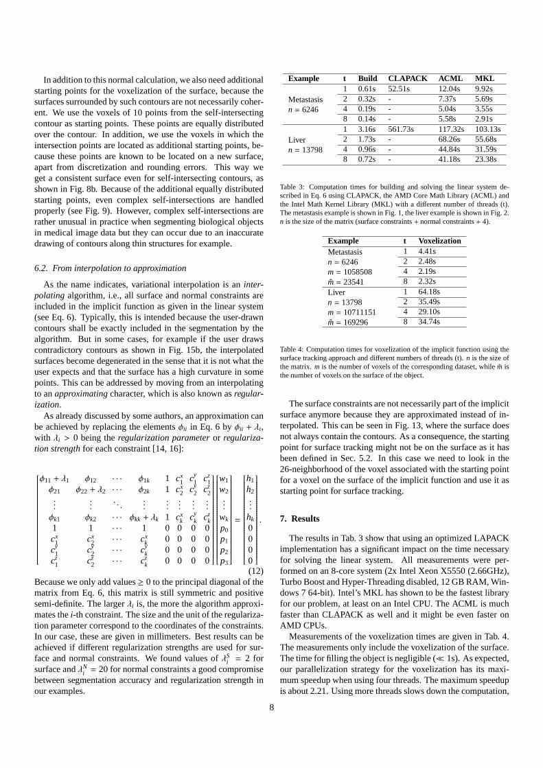
Table 3: Computation times for building and solving the linearsystem de-scribed in Eq. 6 using CLAPACK, the AMD Core Math Library (ACML) andthe Intel Math Kernel Library (MKL) with a different number of threads (t).The metastasis example is shown in Fig. 1, the liver example is shown in Fig. 2.n is the size of the matrix (surface constraints+ normal constraints+ 4).

Example t VoxelizationMetastasisn = 6246m= 1058508m= 23541

1 4.41s2 2.48s4 2.19s8 2.32s

Livern = 13798m= 10711151m= 169296

1 64.18s2 35.49s4 29.10s8 34.74s

Table 4: Computation times for voxelization of the implicit function using thesurface tracking approach and different numbers of threads (t).n is the size ofthe matrix.m is the number of voxels of the corresponding dataset, while ˜m isthe number of voxels on the surface of the object.

The surface constraints are not necessarily part of the implicitsurface anymore because they are approximated instead of in-terpolated. This can be seen in Fig. 13, where the surface doesnot always contain the contours. As a consequence, the startingpoint for surface tracking might not be on the surface as it hasbeen defined in Sec. 5.2. In this case we need to look in the26-neighborhood of the voxel associated with the starting pointfor a voxel on the surface of the implicit function and use it asstarting point for surface tracking.

7. Results

The results in Tab. 3 show that using an optimized LAPACKimplementation has a significant impact on the time necessaryfor solving the linear system. All measurements were per-formed on an 8-core system (2x Intel Xeon X5550 (2.66GHz),Turbo Boost and Hyper-Threading disabled, 12 GB RAM, Win-dows 7 64-bit). Intel’s MKL has shown to be the fastest libraryfor our problem, at least on an Intel CPU. The ACML is muchfaster than CLAPACK as well and it might be even faster onAMD CPUs.

Measurements of the voxelization times are given in Tab. 4.The measurements only include the voxelization of the surface.The time for filling the object is negligible (≪ 1s). As expected,our parallelization strategy for the voxelization has its maxi-mum speedup when using four threads. The maximum speedupis about 2.21. Using more threads slows down the computation,

8

(a) (b)

Figure 10: Example for reducing the number of constraints: (a)shows the orig-inal contours and the result of the interpolation using all 6246 constraints, (b)shows the result after reduction withq = 0.2 resulting in 1390 constraints. Theresulting masks are visually identical.

because the overhead for handling the threads is larger thanthespeedup of the parallel computation as typically only two orfour threads are involved in computations. This is due to thefact that the function values at four or six corners of the voxelhave already been computed during the surface tracking.

However, the results in Tab. 3 and 4 show, that the algorithmdoes not allow real-time response in an interactive segmenta-tion process. Especially in the liver example the segmentationalgorithm is far too slow even with the fastest LAPACK libraryand with parallel voxelization.

Using a proper reduction of the number of constraints yieldsa significant speedup in both solving the linear system andthe voxelization, while resulting in an almost similar overallquality of the segmentation as shown in Tab. 5 and Fig. 10.Calculation times for this preprocessing are negligible (≪ 1s)compared to the overall computations and are not included inTab. 5. The maximum distance between the surface of ini-tial segmentation (i.e., withq = 1.0) and the surface withq = 0.1 corresponds to 2.6% of the maximum diameter forthe metastasis example (which has a maximum diameter of100.8mm) and to 3.3% for the liver example (which has amaximum diameter of 228.643mm). The size of one voxelis (1.086mm,1.086mm,1.0mm) in the metastasis example and(0.66mm,0.66mm,2.0mm) in the liver example, so the maxi-mum distance in Tab. 5 corresponds to about 2.45 voxels forthe metastasis and about 11.31 voxels for the liver. The largemaximum distance in the liver example results from an incor-rect reconstruction due to the use of orthogonal contours (seeFig. 11). Therefore, the bad results for the maximum distancedo not reflect a loss in segmentation quality.

Our measurements show that a real-time response can beachieved for small objects, which allows an interactive segmen-tation. It has also shown that in our current implementationthevoxelization is the main limiting part of the segmentation al-gorithm, which is the reason why the algorithm is not interac-tive for large objects. Solving the linear system is alreadyfastenough, although it has a computational complexity ofO(n3).

Figure 11: Differences in the segmentation result for the liver example whenusingq = 1 (thick light blue contour) andq = 0.1 (thin dark blue contour). Herethe maximum distance between the surfaces is large (about 11 voxels) becauseof a reconstruction issue due to using orthogonal contours (dashed yellow).The result using less contour points (i.e., withq = 0.1) is the more accuratesegmentation.

Example Global Radius Compactly supportedRBFs RBFs

Metastasisn = 6246

1.92s10mm 0.73s20mm 1.40s30mm 2.06s

Livern = 13798

28.95s30mm 12.45s50mm 20.58s70mm 34.82s

Table 6: Voxelization times with 4 threads using compactly supported RBFswith different radii compared to global RBFs forq = 1. A kD-tree was used forfinding all points within the radius of support.

The strength of reduction, i.e., the value ofq, depends onthe actual segmentation task and on the demand for real-timeresponse during the segmentation process. It is a trade-off be-tween reconstruction accuracy and overall calculation time. Inour tests we found a quality of 0.2 ≤ q ≤ 0.5 can be used inmost real-world examples without a loss insubjectivesegmen-tation accuracy.

Results using compactly supported RBFs are shown inFig. 12 and Tab. 6. These results suggest that this class ofRBFs is not suitable for solving our segmentation task. Themain reason for this is, that the constraints generated fromtheuser-drawn contours are rather sparse and thus, a large radiusof support is necessary to generate proper results, which re-duces the theoretical performance of the algorithm significantlyin terms memory consumption, calculation times and segmen-tation quality. Moreover, the objects are not filled correctly ifthe radius is too small, becausef (x) might evaluate to zero forpoints inside the object if their distance to the surface is greaterthan the radius of support. Therefore, a strategy for an auto-matic calculation of the support radius depending on the size ofthe object and the density of the constraints is necessary. How-ever, when using a proper radius, the voxelization step is even

9

Example q n Time Volume overlap Maximum Voxel withsurface distance surface distance > 0

Metastasis

1.0 6246 3.05/2.19 /5.34s 100% 0.0mm 00.5 3552 0.71/1.25 /2.02s 99.94% 1.09mm 980.2 1390 0.08/0.57 /0.69s 99.32% 1.09mm 10300.1 708 0.02/0.39 /0.43s 97.35% 2.63mm 4038

Liver

1.0 13798 24.10/29.10/53.64s 100% 0.0mm 00.5 7892 5.31/18.69/24.18s 99.50% 2.75mm 89160.2 3152 0.55/7.66 /8.33s 98.72% 7.08mm 227700.1 1580 0.11/4.49 /4.71s 97.70% 7.54mm 41012

Table 5: Computation times (linear system building and solving / voxelization/ overall) and segmentation accuracy for different quality settingsq. n is the size ofthe resulting matrix. For all measurements the MKL with 8 threads and the voxelization with 4 threads were used. Volume overlap (Jaccard index) and surfacedistance are given relative to the interpolation result with q = 1. The overlap is calculated by the number of intersecting voxels divided by the number of voxels inthe union of two segmentations. The minimum surface distance was 0mm for all cases.

(a) (b) (c)

(d) (e) (f)

Figure 12: Results using RBFs with compact support of different radii (in-dicated by the black circle) forq = 1: (a) Metastasis withα = 10mm, (b)α = 20mm and (c)α = 30mm. (d) Liver withα = 30mm, (e)α = 50mm and(f) α = 70mm. Using a smaller radius, the surface becomes more “bumpy”.Only (c) and (f) have been filled correctly by the voxelization. The arrowsindicate some main differences of the resulting segmentations.

slower for our segmentation problems when using RBFs withcompact support compared to the global interpolation approach.

As shown in the examples in Fig. 13, the robustness ofthe segmentation algorithm can further be improved by mov-ing from an interpolating to an approximating reconstructionscheme. By using approximation instead of interpolation, con-tradictory user-drawn contours and contours with high curva-ture can be segmented more robustly for instance. Therefore,approximation generates better segmentations than interpola-tion in our opinion. Because we only add constants to the ele-ments on the principal diagonal of the matrix in Eq. 12, this ap-proach does not affect the time necessary for solving the linearsystem. Because with approximation a little less voxels areonthe surface of the segmentation, the voxelization time is slightlyreduced in practice.

(a) (b) (c)

Figure 13: Comparison between interpolation and approximation with differentregularization strengths for the liver example: (a) interpolation, (b) approxi-mation withλS

i = 2 andλNi = 20 and (c) approximation withλS

i = 50 andλN

i = 100. The arrows indicate the main differences of the resulting segmenta-tions.

8. Evaluation

For evaluation of our algorithm, we have developed a toolusing MeVisLab6 that allows a slice-wise manual segmenta-tion in axial view, a segmentation using variational interpola-tion with only parallel axial contours and a segmentation us-ing variational interpolation with contours in axial, sagittal andcoronal orientation. Figure 14 shows this tool. Our evaluationtool measures the time that is necessary for segmentation andit tracks the number of contours that are needed. Moreover,it allows to rate the segmentation quality and the segmentationtime on a scale between 1 and 5, with 1 being “bad” and 5 being“perfect”.

Our algorithm was evaluated by two experienced radiologytechnicians on 15 liver metastases of different size (rangingfrom 0.05ml to 53.26ml) and complexity and 1 liver. The PCused for evaluation was a Windows 7 64-bit system with an IntelCore 2 Duo E6850 (3.0GHz) and 8GB RAM. Thus, only twothreads were used for computation. For contouring, a touch-screen display with a pencil-like input device was used. Thequality factor for constraint reduction was set toq = 0.2, whilethe regularization strengths were set toλS

i = 2 andλNi = 20.

6MeVisLab: http://www.mevislab.de

10

Manual Variational interpolation Variational interpolation(axial) (axial) (axial, sagittal, coronal)

Metastases

Time 111.4s 64.2s 70.5sNumber of contours 20.6 7.1 5.2Number of steps 29.3 8.2 5.4Quality rating 4.9 3.8 4.0Time rating 3.8 4.0 4.1Overlap to manual segmentation 100% 75.77% 71.54%Maximum surface distance 0 2.94mm 3.69mmNumber of voxels with distance> 0 0 2313 3340

Liver

Time 1272.5s 665s 734.5sNumber of contours 106 22 20.5Number of steps 148.5 32 25Quality rating 5 3 4.5Time rating 2.5 3.5 4.5Overlap to manual segmentation 100% 93.98% 92.68%Maximum surface distance 0 9.37mm 10.12mmNumber of voxels with distance> 0 0 105101 128250

Table 7: Results of the evaluation of our algorithm for segmentation of 15 liver metastases and 1 liver by 2 experienced radiology technicians. All results are givenas average over all cases and participants. The overlap and distance measures are given relative to the manual segmentation.

Figure 14: The tool used for evaluation of our algorithm. The user-drawncontours are shown in yellow. The surface of the interpolated segmentationis shown in blue.

Table 7 gives an overview on the results of our evaluation. Astep refers to drawing, deleting or editing a contour.

Our evaluation shows that using variational interpolation, thesegmentation times can be reduced by a factor of about 2. Com-pared to the number of contours used for the manual segmenta-tions, only one fifth to one third of the contours are necessarywhen using our interpolation algorithm, depending on the seg-mentation task. The fact that the segmentation takes only halfas long although about one fourth of the contours are necessarycan be explained by the time the variational interpolation needsfor computation and by the interactive process. This process re-quires an assessment of the current segmentation result andtheuser might need to correct or even delete already drawn con-tours. The assessment is known to take almost as much time

as manually drawing contours. Unfortunately, the segmenta-tion quality has been rated slightly worse compared manualsegmentations. This also corresponds with the accuracy of oursegmentation algorithm in terms of the volume overlap and themaximum surface distance compared to the manual segmenta-tions. By using orthogonal contours instead of only parallelaxial contours, the number of contours necessary for segmenta-tion can further be reduced, although the overall segmentationtime increases, probably due to the more time intensive taskof looking at different views. The benefit of using contours indifferent views was emphasized by the radiology techniciansin particular for sphere-shaped structures. For objects with amore complex and irregular shape, drawing contours in differ-ent views was assessed as rather counterproductive.

Although we have not yet compared our algorithm to moreadvanced contour-based semi-automatic segmentation algo-rithms like live-wire, we expect a speedup in the segmenta-tion time that is comparable to the speedup measured for puremanual segmentations, because variational interpolationcan becombined with such approaches as well. However, it would beinteresting to compare variational interpolation with thecombi-nation of live-wire and a shape-based interpolation as suggestedby Schenket al. [31].

9. Discussion and future work

As shown in the examples, variational interpolation allowsa smooth segmentation of objects in medical images from asparse set of contours (see Fig. 1 and Fig. 2). The algorithmis computationally expensive and needs much memory (O(n2)),because it is a global interpolation. Therefore, the numberofconstraints is limited by the available memory. Moreover, com-putation times are slow for a large number of constraints. Thiscan be solved by reducing the constraints resulting in compu-tation times that allow a real-time response for segmentation of

11

Direct Fast multipoleStorage O(n2) O(n)Setup - O(n logn)Linear system solving O(n3) O(n logn)Evaluation per point O(n) O(1)

Table 8: Complexity of different steps of the algorithm when using the directmethod and the fast multipole method according to Carret al. [13].

(a) (b) (c)

Figure 15: Limitations of our algorithm: (a) 2D normal constraints using inter-polation (which can be seen at the uneven silhouette), (b) contradictory contour(red) in the liver example and (c) a square-shaped contour being interpolated toa sphere.

small objects like a tumor in an interactive segmentation pro-cess. However, in our current implementation and for large ob-jects like the liver, the voxelization becomes the bottleneck afterconstraint reduction and the algorithm does no longer allowareal-time response.

Our goal is to allow an interactive segmentation even forlarge objects like the liver. Therefore, future work will focuson reducing the voxelization times by using an improved paral-lelization strategy. We will also evaluate, whether GPU-basedimplementations can improve computation times significantly.For further improving the performance and reducing the mem-ory consumption of the algorithm we will also investigate thefast multipole methodwhich has been suggested by Carret al.[13]. The fast multipole method allows solving the variationalinterpolation problem with reduced complexity in both the re-quired memory and the calculation time (see Tab. 8). Becausethis method can be seen as a global reconstruction approachit does not have the drawbacks of compactly supported RBFs.Therefore, it should be better suited for solving our 3D segmen-tation problem.

The presented algorithm still has some limitations concern-ing the segmentation quality. Normal constraints are currentlycomputed based on a single contour, i.e., in 2D. But neighbor-ing contours influence the normal of the surface as well (seeFig. 15a). This can be slightly compensated when using ap-proximation instead of interpolation. Another issue are contra-dictory contours, i.e., contours that define different surfaces, al-though they should be located on the same surface. This can inparticular happen for non-parallel contours like in the liver ex-ample, as shown in Fig. 15b (the figure shows the same part ofthe liver segmentation that is shown in the bottom row of Fig.13but from another point of view). A similar example that resultsfrom a combination of both of these issues has already beenshown in Fig. 11. Although this can be compensated by an ap-

Figure 16: Erroneous reconstruction of an object with high curvature with aninsufficient number of constraints because of parallel contours with low overlapand low distance. The example was taken from a 3D microscopy dataset.

(a) (b)

Figure 17: Example for cutting out a part of the segmentation where the algo-rithm fails because of its single-contour-based normal calculation: (a) result ofour algorithm and (b) the expected result.

proximation as well (see Sec. 6.2), a more advanced handling,like an additional preprocessing step that solves such inconsis-tencies or user-guidance during contour-drawing, is essentialfor consistent results according to the expectations of theuser.We will investigate this in the future. Furthermore, the regu-larization parameters of the approximation need to be furtherevaluated. For example, it might be advantageous to computedan individual regularization strength for each constraintbasedon a contours shape or complexity.

A conceptual drawback of the smooth interpolation is that theresulting surface does not always look like how the user wouldexpect it if the number of constraints is too low. For example, asquare-shaped contour that is only defined by its corner pointswill be interpolated to a sphere using the presented algorithm(see Fig. 15c). For objects with high curvature the reconstruc-tion might fail, if the surface is sampled too sparse, i.e., with notenough contours. This can also be the case if parallel contoursare close the each other and the overlap between the contoursislow. Figure 16 shows such a situation.

Because of the way how normal constraints are computed,which is done per contour (see Sec. 4.1), it is not possible tocutout an inner part of an object as shown in Fig. 17 because thereconstruction algorithm has no information on what shouldbeincluded into the segmentation and what should be excluded.Instead, this needs to be solved on the interface level, so theuser has the possibility to explicitly define parts that should beremoved from the segmentation.

Finally, we think of combining the reconstruction algorithmwith image information to allow more accurate segmentations,e.g., by image-adaptive RBFs described by Mory and Ardon[30].

12

10. Conclusion

Variational interpolation allows an accurate and robust recon-struction of the surface of an object defined by a set of planarcontours that can be arbitrarily oriented in 3D space. A surfacegenerated using variational interpolation is smooth, it isguaran-teed that all used contour points are part of the surface and theresulting surface is plausibly extrapolated into regions where nocontours have been drawn. Thus, the algorithm is well suitedfor supporting the segmentation of objects in medical imagesin a contour-based workflow. Because it is independent of im-age information, the algorithm can be used for any 3D modality(e.g., CT, MRI, 3D US) and it can also be used for segmenta-tion of objects with no contrast to the background. In addition,the interpolation can easily be extended to more dimensions,which would allow an interpolation of an object over severaltime points as well for example.

Although the algorithm is time and memory consuming, cal-culation times can be significantly decreased using modernCPU features and a reduction of the number of constraints. Be-cause segmentation is done using contours, a fast and robustre-duction strategy can be used, that preservers the shape of eachcontour. This way, the differences in the interpolated resultsare visually not distinguishable from the result using all con-tour points. As a result, the algorithm allows a real-time re-sponse for small objects, which enables an interactive segmen-tation process. Using approximation instead of interpolationimproves the robustness of the segmentation algorithm in theliver example while it does not increase calculation times.

The local interpolation scheme, which uses RBFs with com-pact support, is not suitable for the presented segmentationproblems, because the constraints generated from the user-drawn contours are too sparse and thus the radius of supportneeds to be too large.

Our evaluation has shown that using variational interpolationcan reduce segmentation times by a factor of about 2. We as-sume that this factor increases as the user gets more familiarwith the segmentation tool and, especially for large objects likethe liver, as the algorithm itself becomes faster.

Acknowledgment

We thank Christiane Engel and Ulrike Kayser from Fraun-hofer MEVIS for evaluating our algorithm. Parts of this workwere funded by Siemens AG, Healthcare Sector, Imaging &Therapy Division, Computed Tomography, Forchheim, Ger-many.

Appendix A. Algorithm overview

Algorithm 1: Segmentation using variational interpolationData: Contours, quality factor, reference imageResult: SegmentationPerform constraint reduction;Perform variational interpolation;Perform voxelization;

Function Constraint reductionData: Contours, quality factorResult: Contoursforeach User drawn contour Ci do

foreach Contour pointci doCompute weightωi ;

endwhile #points exceeds quality factor qdo

Remove point with lowest weight;Update weights of the adjacent points;

endCompute average line segment length;foreach Line segmentdo

if Length> 2× average lengththenInsert additional points;

endend

end

Function Variational interpolationData: ContoursResult: Implicit function, starting pointsforeach User drawn contour Ci do

Find point with minimum x-, y- or z-coordinate;Initialize sign for normal;foreach Contour pointcS

i starting from minimum pointdoCheck adjacent line segment for self-intersections;if Number of self-intersections is oddthen

Invert sign for normal;endCompute normalni and normal constraintcN

i ;end

endBuild matrix for Eq. 6 in parallel;Solve Eq. 6 using LAPACK to getf (x);

Function VoxelizationData: Implicit function, starting points, reference imageResult: Segmentationforeach Starting pointdo

Evaluatef (x) at each corner point;if Voxel of starting point is not on surface of f(x) then

Check voxels in 26-neighborhood;endif Starting voxel is not on any already voxelized surfacethen

repeatEvaluatef (x) at each corner of the voxel in parallel(= configuration);Move to next voxel in 6-neighborhood depending onthe configuration;

until Surface is voxelized;end

endforeach Slice of the resulting imagedo

foreach Row of the slicedoFill surface;

endend

13

References

[1] Hahn, H.K., Peitgen, H.O.. IWT - interactive watershed transform: Ahierarchical method for efficient interactive and automated segmentationof multidimensional gray-scale images. In: Sonka, M., Fitzpatrick, J.M.,editors. SPIE Medical Imaging: Image Processing; vol. 5032. SPIE; 2003,p. 643–653. doi:10.1117/12.481097.

[2] Grady, L.. Random walks for image segmentation. IEEE Transactionson Pattern Analysis and Machine Intelligence 2006;28(11):1768–1783.doi:10.1109/TPAMI.2006.233.

[3] Cohen, L.D.. On active contour models and balloons. CVGIP: ImageUnderstanding 1991;53:211–218. doi:10.1016/1049-9660(91)90028-N.

[4] Barrett, W.A., Mortensen, E.N.. Interactive live-wireboundary extrac-tion. Medical Image Analysis 1997;1:331–341.

[5] Bredno, J., Lehmann, T.M., Spitzer, K.. A general discrete contourmodel in two, three, and four dimensions for topology-adaptive multi-channel segmentation. IEEE Transactions on Pattern Analysis and Ma-chine Intelligence 2003;25:550–563. doi:10.1109/TPAMI.2003.1195990.

[6] McInerney, T.. SketchSnakes: Sketch-line initializedsnakesfor efficient interactive medical image segmentation. Computer-ized Medical Imaging and Graphics 2008;32(5):331–352. doi:10.1016/j.compmedimag.2007.11.004.

[7] Turk, G., Dinh, H.Q., O’Brien, J., Yngve, G.. Implicit sur-faces that interpolate. In: International Conference on Shape Model-ing and Applications. IEEE Computer Society; 2001, p. 62–71.doi:10.1109/SMA.2001.923376.

[8] Raya, S.P., Udupa, J.K.. Shape-based interpolation of multidimensionalobjects. IEEE Transactions on Medical Imaging 1990;9(1):32–42. doi:10.1109/42.52980.

[9] Olabarriaga, S.D., Smeulders, A.W.M.. Interaction in the segmentationof medical images: A survey. Medical Image Analysis 2001;5:127–142.

[10] Preim, B., Dachselt, R.. Interaktive Systeme 1: Grundlagen, Graph-ical User Interfaces, Informationsvisualisierung, MobileInteraktion.Springer; 2 ed.; 2010.

[11] Turk, G., O’Brien, J.F.. Shape transformation using variational implicitfunctions. In: ACM SIGGRAPH. ACM. ISBN 0-201-48560-5; 1999, p.335–342. doi:10.1145/311535.311580.

[12] Turk, G., O’Brien, J.F.. Modelling with implicit surfaces that in-terpolate. ACM Transactions on Graphics 2002;21(4):855–873. doi:10.1145/571647.571650.

[13] Carr, J.C., Beatson, R.K., Cherrie, J.B., Mitchell, T.J., Fright, W.R.,McCallum, B.C., et al. Reconstruction and representation of3D objectswith radial basis functions. In: ACM SIGGRAPH. ACM. ISBN 1-58113-374-X; 2001, p. 67–76. doi:10.1145/383259.383266.

[14] Dinh, H.Q., Turk, G., Slabaugh, G.. Reconstructing surfaces by volu-metric regularization using radial basis functions. IEEE Transactions onPattern Analysis and Machine Intelligence 2002;24(10):1358–1371. doi:10.1109/TPAMI.2002.1039207.

[15] Carr, J.C., Beatson, R.K., McCallum, B.C., Fright, W.R., McLennan,T.J., Mitchell, T.J.. Smooth surface reconstruction from noisy range data.In: International conference on Computer graphics and interactive tech-niques in Australasia and South East Asia. ACM. ISBN 1-58113-578-5;2003, p. 119–126. doi:10.1145/604471.604495.

[16] Yngve, G., Turk, G.. Robust creation of implicit surfaces from polygo-nal meshes. IEEE Transactions on Vizualization and Computer Graphics2002;8(4):346–359.

[17] Ohtake, Y., Belyaev, A., Seidel, H.P.. 3D scattered data interpolationand approximation with multilevel compactly supported RBFs. GraphicalModels 2005;67(3):150–165. doi:10.1016/j.gmod.2004.06.003. SpecialIssue on SMI 2003.

[18] Walder, C., Scholkopf, B., Chapelle, O.. Implicit surface modelling witha globally regularised basis of compact support. In: ComputerGraphicsForum (Proceedings of Eurographics). Eurographics Association; 2006,p. 635–644.

[19] Morse, B.S., Yoo, T.S., Rheingans, P., Chen, D.T., Subramanian, K.R..Interpolating implicit surfaces from scattered surface data using com-pactly supported radial basis functions. In: ACM SIGGRAPH Courses.ACM; 2005, p. 78–87. doi:10.1145/1198555.1198645.

[20] Sußmuth, J., Meyer, Q., Greiner, G.. Surface reconstruction based onhierarchical floating radial basis functions. Computer Graphics Forum2010;29(6):1854–1864. doi:10.1111/j.1467-8659.2010.01653.x.

[21] Rohr, K.. Landmark-Based Image Analysis: Using Geometricand In-tensity Models. Springer Netherlands; 2001. ISBN 0792367510.

[22] Modersitzki, J.. Numerical Methods for Image Registration. OxfordUniversity Press; 2003.

[23] Morse, B., Liu, W., Yoo, T., Subramanian, K.. Active contours usinga constraint-based implicit representation. In: IEEE Conference on Com-puter Vision and Pattern Recognition; vol. 1. IEEE Computer Society;2005, p. 285–292. doi:10.1109/CVPR.2005.59.

[24] Slabaugh, G., Dinh, Q., Unal, G.. A variational approach to the evo-lution of radial basis functions for image segmentation. In: IEEE Con-ference on Computer Vision and Pattern Recognition. IEEE ComputerSociety; 2007, p. 1–8. doi:10.1109/CVPR.2007.383013.

[25] Freedman, D., Radke, R., Zhang, T., Jeong, Y., Lovelock,D., Chen,G.. Model-based segmentation of medical imagery by matching distri-butions. IEEE Transactions on Medical Imaging 2005;24(3):281–292.doi:10.1109/TMI.2004.841228.

[26] Gelas, A., Bernard, O., Friboulet, D., Prost, R.. Compactly sup-ported radial basis functions based collocation method for level-set evo-lution in image segmentation. IEEE Transactions on Image Processing2007;16(7):1873–1887. doi:10.1109/TIP.2007.898969.

[27] Wimmer, A., Soza, G., Hornegger, J.. Two-stage semi-automatic organsegmentation framework using radial basis functions and level sets. In:3D Segmentation in The Clinic: A Grand Challenge, MICCAI Workshop.Springer; 2007, p. 179–188.

[28] Carr, J.C., Fright, W.R., Beatson, R.K.. Surface interpolation withradial basis functions for medical imaging. IEEE Transactions on MedicalImaging 1997;16:96–107.

[29] Masutani, Y.. RBF-based representation of volumetric data: Applica-tion in visualization and segmentation. In: Dohi, T., Kikinis, R., ed-itors. International Conference on Medical Image Computing and Com-puter Assisted Intervention; vol. 2489 ofLecture Notes in Computer Sci-ence. Springer Berlin/Heidelberg; 2002, p. 300–307. doi:10.1007/3-540-45787-938.

[30] Mory, B., Ardon, R., Yezzi, A., Thiran, J.P.. Non-euclidean image-adaptive radial basis functions for 3D interactive segmentation. In: IEEEInternational Conference on Computer Vision. IEEE Computer Society;2009, p. 787–794. doi:10.1109/ICCV.2009.5459245.

[31] Schenk, A., Prause, G.P.M., Peitgen, H.O.. Efficient semiautomaticsegmentation of 3D objects in medical images. In: International Confer-ence on Medical Image Computing and Computer Assisted Intervention.Springer-Verlag. ISBN 3-540-41189-5; 2000, p. 186–195.

[32] de Bruin, P.W., Dercksen, V.J., Post, F.H., Vossepoel,A.M., Streekstra,G.J., Vos, F.M.. Interactive 3D segmentation using connected orthogonalcontours. Computers in Biology and Medicine 2005;35(4):329–346. doi:10.1016/j.compbiomed.2004.02.006.

[33] Liu, L., Bajaj, C., Deasy, J.O., Low, D.A., Ju, T.. Surface reconstruc-tion from non-parallel curve networks. In: Computer Graphics Forum(Proceedings of Eurographics); vol. 27. Eurographics Association; 2008,p. 155–163.

[34] Haines, E.. Graphics Gems IV; chap. Point in Polygon Strategies. Aca-demic Press, Inc.; 1994, p. 24–48.

[35] Bunch, J.R., Kaufman, L., Parlett, B.N.. Decomposition of a symmetricmatrix. Numerische Mathematik 1976;27:95–109.

[36] Newman, T.S., Yi, H.. A survey of the marching cubes algorithm. Com-puters & Graphics 2006;30(5):854–879. doi:10.1016/j.cag.2006.07.021.

[37] Wyvill, G., McPheeters, C., Wyvill, B.. Data structurefor sof objects.The Visual Computer 1986;2:227–234. doi:10.1007/BF01900346.

[38] Latecki, L.J., Lakamper, R.. Convexity rule for shape decompositionbased on discrete contour evolution. Computer Vision and Image Under-standing 1999;73:441–454.

[39] Goodman, J.E., O’Rourke, J., editors. Handbook of Discrete and Com-putational Geometry. Chapman & Hall; 2 ed.; 2004.

[40] Horritt, M.S.. A statistical active contour model for SAR image seg-mentation. Image and Vision Computing 1999;17(3–4):213–224.doi:10.1016/S0262-8856(98)00101-2.

14