INTERACTIVE AIRCRAFT FLIGHT CONTROL AN D

AEROELASTIC STABILIZATION

NASA/Langley Research Center Grant-NAG-1 - 157

Semi-annual Report

1 Yay 1985 through 31 October 1985

Submitted by:

Dr. Terrence A . Weisshaar

Principal Investigator

SCHOOL OF AERONAUTICS ANT) ASTrlO~lAllT ICs

PURLUE UNIVEKSITY

VEST LAFAYETTE, INDIANA 47907

No vemhe r 1985

(UASA-CB-176323) INTERACTIVE AIRCRAFT N86- 12233

FLIGHT CONTROL A10 A E b O E L A S T I C S T A B U I Z A I I O N Semiannual RepOKt, 1 aay - 3 1 Oct. 1985 [Purdue U n i v . ) 48 p HC A 0 3 / B F A 3 1 CSCL 01C Unclas

63/08 04773

https://ntrs.nasa.gov/search.jsp?R=19860002766 2018-05-22T07:20:06+00:00Z

2

1.0 Sunmary

This r epor t covers a c t i v i t y dur ing t h e time pertod 1 May 1985

through 31 October 1985.

graduate s tudents were supported by t h i s grant . One s t u d e n t , Hr. James

S a l l c e spent 10 ueeks in-residence a t NASA Langley as p a r t of h i s gradL

ate t r a in ing . A second s tuden t , Mr. Thomas Zeilcr received h i s Ph.0.

degree from Purdue i n August 1985.

sored by t h e Grant. The P r i n c i p a l I n v e s t i g a t o r spent one week in-

res idence a t NASA/Langley during June 1985.

t a l k a t t h e Aerospace F l u t t e r and Dynamics Council Semi-annual meeting

i n A t l a n t i c Ci ty , New J e r s e y i n October 1985. A por t ion of Mr. Zeiler's

d i s s e r t a t i o n work has been submitted fo r cons idera t ion for t h e A I A A SDX

Meeting t o be held i n San Antonio, Texas i n May 1986.

During t h i s t i m e one f a c u l t y member and two

His graduate d i s s e r t a t i o n was spon-

I n addi t ion , he presented a

This r epor t b r i e € l y descr ihes research completed by D r . Zeiler and

Professor Weisshaar. A copy of D r . Zeiler's d i s s e r t a t i o n has been for-

warded t o the cont rac t monitor. The proposal for the SDM paper is con-

ta ined i n the Appendix. I n a d d i t i o n , the preliminary work by Mr. S a l l e e

and ProEessor Weisshaar is discussed. A d e t a i l e d expos i t ion of t h a t

work is also contained i n t h e Appendix.

3

2.0 krost.rvoelastic Optimization Studies

A preliminary study of atroservoelastic optimization techniques was

completed in August 1985.

a methodology for maximization of the stable flight envelope of an

idealized, actively controlled, flexible airfoil. The equations of

motion for the airfoil were developed in state-space form to include

time-domain representations of aerodynamic forces and active control.

For optimization, the shear center position was taken to be a design

variable. Optimal, steady-state, linear-quadratic regulator theory

(SSLQR) was used for control law synthesis.

The objective of this study was to deternine

The synthesis of feedback control laws uith SSLOR theory can

present problems. One recurring problem is that a system may be stabil-

ized actively at a certain design airspeed (or a nondimensional counter-

part, UDEs) but may be unstable at lawer, off-design airspeeds. This

peculiarity necessitated the development of an optimization scheme to

stabilize the aetoelastic system over a range of airspeeds, including

the design airspeed. This requirement led to an integrated or multi-

disciplinary approach that was demonstrated to be beneficial.

-

Dr. Ztiler organized his solution approach into two levels, one at

the "system" level, the other at the "subsystem" level. The subsystems

are: (a) the airfoil structure, with a design variable represented by

the shear center position; and, (b) the control system. An objective

vas stated io mathematical form and a search was conducted wfth the res-

triction that each subsystem be constrained to be optimal in some sense.

To implement the procedure, analytical expressions were deuloped

to compute the changes in the eigenvalues of the closed-loop, actively

controlled system. A stability index was constructed to ensure that

4

s t a b i l i t y was present at t h e design speed and a t other a i r s p e e d s away

from t h e design speed.

The design Frocedurc begins wlth t h e choice of i n i t i a l values of

shear c e n t e r pos i t ion , design a i r speed and o t h e r c o n t r o l r e l a t e d parame-

ters. A feedback c o n t r o l l a w is then synthesized and t h e a i r speed

envelope is checked for s t a b i l i t y by computing t h e value of t h e s tabi l -

i t y index.

unstable. The approach relies on a procedure to reduce t h e value of t h e

s t a b i l i t y index below z e r o ( t o achieve stability) i n an opt imal manner.

This procedure was demonstrated to be e f f e c t i v e . Mathematical r e s u l t s

were explained i n a physical context .

When t h e s t a b i l i t y index is p o s i t i v e , the system is

The above study and t h e procedure used is descr ibed In d e t a i l i n

t h e Ph.r). d i s s e r t a t i o n "An Approach t o In tegra ted Aeroservoelast ic

Ta i lor ing for S t a b i l i t y " by T.A. Zeiler. This s tudy is notahle because

i t i n d i c a t e s - a procedure (no t - t h e procedure) f o r a successfu l i t e r a t i v e

s t r u c t u r e s / c o n t r o l design modification. It has a rea l i s t ic measure of

performance ( i n s t a b i l i t y freedom a t and within t h e l a r g e s t poss ib le

design envelope). It also i l l u s t r a t e s how one might organize t h e s t ruc-

t u r a l design and c o n t r o l design procedures In a l o g i c a l way.

5

3.0 h r r e n t Aeroservoelast ic T a i l o r i n g S tudies

The study descr ibed i n Sect ion 2.0 and t h e experience gained from

those S t u d i e s has enabled t h e P r i n c i p a l I n v e s t i g a t o r to mow t o t h e next

level of e f f o r t . This e f f o r t inc ludes a more realistic s t r u c t u r a l

model, incorpora t ing t h e inf luence of advanced composite materials. I n

a d d i t i o n , t h e e f f o r t inc ludes t h e use of 3-D unsteady aerodynamic

e f f e c t s and classical c o n t r o l procedures (as opposed to optimal c o n t r o l

procedures) . This e f f o r t is c u r r e n t l y i n a prel iminary s tage.

a h ighly idea l ized a n a l y t i c a l model has been developed t o e f f i c i e n t l y

include the e f f e c t of d i r e c t i o n a l s t i f f n e s s such as might be present i n

laminated s t r u c t u r e s . This model a l s o has educat ional value as ell as

research s igni f icance . A computer program has also been developed t o

perform f l u t t e r c a l c u l a t i o n s on both the open-loop and closed-lc ;ys-

terns. In addi t ion , t h e program can compute " s e n s i t i v i t y der iva t ives"

with respect t o a v a r i e t y of system design var iah les such as s t i f f n e s s

and feedback c o n t r o l gains . These s e n s i t i v i t y d e r i v a t i v e s a r e necessary

f o r system redesign procedures.

A s a f i r s t s t e p ,

The model i s a l s o usefu l as an educat ional t o o l t o demonstrate to

s t u d e n t s and profess iona ls t h e var ious o p p o r t u n i t i e s afforded by

i n t e g r a t e d design.

S a l l e e under t h e d i r e c t i o n of Professor Weisshaar. The c u r r e n t s t a t u s

of t h e a n a l y s i s and a d e t a i l e d model d e s c r i p t i o n and development is con-

t a i n e d i n t h e Appendix to t h i s r epor t . This port ion of t h e e f f o r t l e

due f o r completion at t h e end of t h i s year. A t t h a t time a more

d e t a i l e d , multi-mode a n a l y t i c a l model w i l l be implemented t o f u r t h e r

i n v e s t i g a t e i n t e r e s t i n g f e a t u r e s revealed by t h e i n i t i a l model.

The model development has been done by Mr. James

6

4.0 Future Work

This semi-annual period of t h e g ran t has produced r e s u l t s beyond

expectat ion. One Ph.D. s tudent , well-schooled i n both c o n t r o l methodol-

ogy, s t r u c t u r a l dynamics and a e r o e l a s t i c i t y and opt imiza t ion methods has

been graduated and has joined t h e ranks of American aerospace workers.

This event would n o t have occurred without NASA research sponsorship.

The r e s u l t s of t h e research e f f o r t produced by t h i s s tudy are s i g n i f i -

c a n t and far-reaching. A new s tudent has begun t o delve i n t o t h e suh-

ject where the o t h e r l e f t o f f .

The i d e a l i z a t i o n descr ibed i n t h e Appendix w i l l be used t o survey,

i n a prelimlnary manner, several of t h e more i n t e r e s t i n g r e s u l t s

obtained from T k . Zeiler’s d l s s e r t a t € o n . In p a r t i c u l a r , t h e e f f e c t s of

s t i f f n e s s cross-coupling on a c t i v e c o n t r o l are of i n t e r e s t i n t h e

c u r r e n t work.

t h a t which preceded i t w i l l be the design methodology f o r t h e a c t i v e

c o n t r o l i t s e l f .

An a d d i t i o n a l d i f f e r e n c e between t h e c u r r e n t s tudy and

A l a r g e por t ion of t he next research period w i l l be spent develop-

i n g a modal model of a swept wing design.

a t tempt t o have remote use of I S A C via a h tdue /Langley phone hookup.

T h i s e f f o r t w i l l be continued with H r . S a l l e e in-residence a t

E?ASA/Langley , beginning i n May 1986 .

For t h i s s tudy we w i l l

APPENDIX A

Proposed SDM Presentation

Integrated Aeroservoelastic

Tailoring of Lifting Surfaces

Thomas A. Zeiler* Kentron International, Inc. Hampton Technical Center 3221 N. Armistead Ave. Hampton, Virginia 23666

Phone 804-838-1010

and

- Terrence A. Weisshaar* School of Aeronautics and Astronautics

Pur due University West Lafayette, Indiana 47907

Phone 317-494-5975

Abstract of Paper Proposed for the

27th AIAA Structures, Structural Dynamics

and Materials Conf erencet

May 1986

San Antonio, Texas

*Members, AIAA Address all correspondence to the second author. tProposed for the Structural Dynamics session.

2

The design of an aerospace structure involves a complicated

sequence of operations requiring multiple, interdisciplinary interac-

tions. The overall design process has a single objective, superior per-

formance subject to a multitude of constraints. Unfortunately, perfor-

mance has a multiplicity of definitions, depending upon the specific

discipline involved within the design process. Worse yet, sometimes

these measures of performance are at odds with one another. Future com-

petitive aerospace structural designs Will increase the need for

creative interaction among the various disciplines and also require

accounting for these interactions early in the desfgn process.

paper will discuss the integration of two of these areas, the optimal

This

design'process for structures and active control of such a structure.

While the results presented are limited in scope, they nonetheless

illustrate benefits of integrating the aeroservoelastic design process.

This integrated design process is referred to as integrated aeroservoe-

lastic tailoring.

The objective of this study was to determine how to maximize the

stable flight envelope of an idealized, actively controlled aeroelastic

system shown in Figure 1. This 4-degree-of-freedom system consists of a

3-degree-of-freedom, typical-section airfoil mounted on a rigid support

with a stabilizing tail surface; the model is free to pitch about a

pivot. This model is Intended to simulate a flexible wing with an

important body freedom. This model has the potential for simulating

high frequency classical flutter behavior, low frequency body-freedom

flutter and classical divergence.

An analytical formulation of the equations of motion of this model

was developed, including unsteady aerodynamic loads in an s-plane or

3

time domain form. The result was a state-space representation of the

equations of motion. The structural design variable was taken to be the

shear center position with respect to the airfoil midchord, denoted as

a in Figure 1.

airfoil semi-chord dimension, b, and is taken to be positive if the

This parameter is nondimensional with respect to the e

shear center lies aft of the airfofl midchord.

to a are -1 < ae < 1.

As a result, the limits

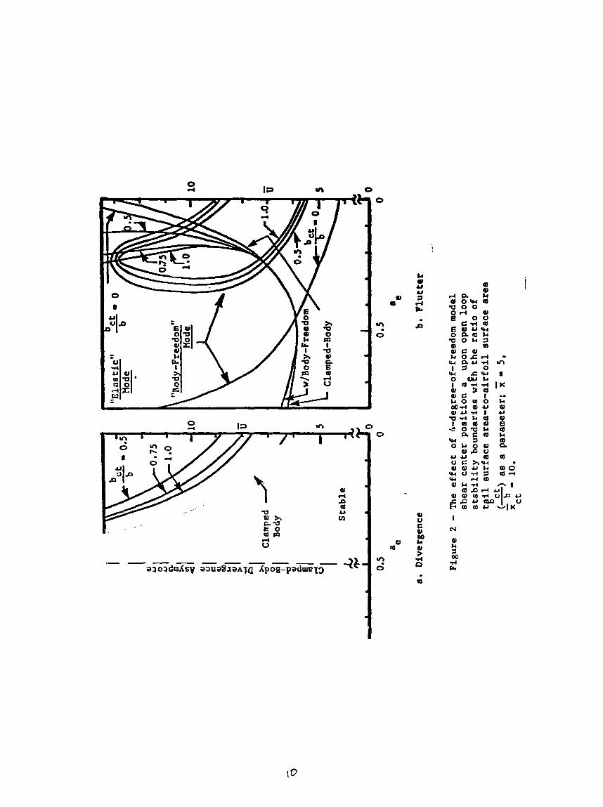
e Optimal steady-state linear quadratic regulator theory (SSLQR) was

used to synthesize full-state fee6back control laws to stabilize the

model at different airspeeds (represented in nondimensional form as

'DES e control-off, stability boundaries for the model dimensions chosen, but

- ) and different values of a . Figure 2 shows the "open-loop",

with a

trarily.

surface area to wing surface area.

taken to be a design parameter capable of being chosen arbi- e In Figure 2, the parameter bCT/b represents the ratio of tail

Note that full body pitch restraint

or "clamping" the fuselage reduces the flutter and divergence boundaries

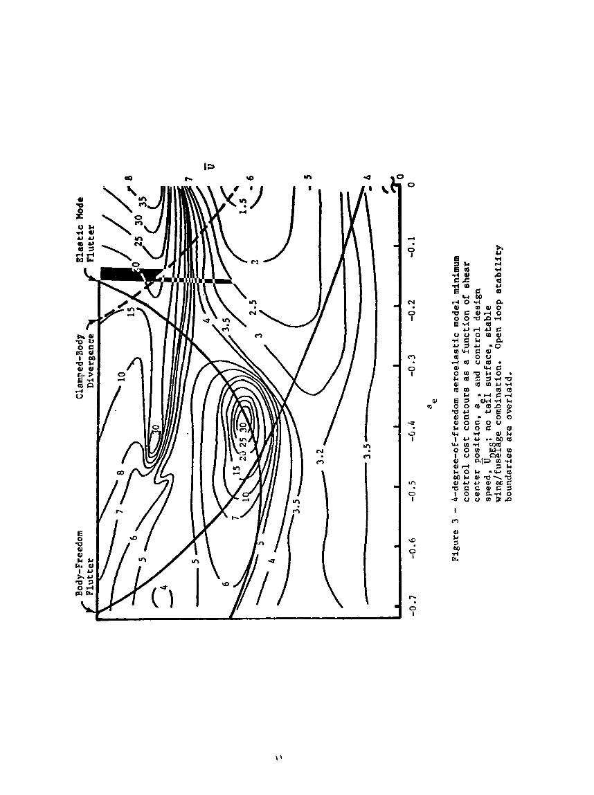
to those of the 3-degree-of-freedom airfoil alone. The use of SSLQR

theory to synthesize control laws with the shear center at various posi-

tions uses a measure of state and control activity at a fixed design

airspeed, i?

function J for this idealization are plotted versus a and design e While the absolute value of J has no phy- airspeed,

sical significance, the relatively large valws of J near a = -0.4 and

as a cost function, J, to be minimized. Values of this DES '

- i n Figure 3. 'DES 9

e - = 6 indicate that the active control is experiencing difficulty 'DES

stabilizing the system fn this region.

These regions of relatively high cost correspond to configurations

for which the system experiences near-uncontrollability of unstable

4

aodes. This is indicated in Figure 4 by the close proximity of zeros of

the loop transfer matrix to some system poles (eigenvalues) near the j w

axis.

A similar contour plot for control cost was constructed for the

airfoil model with rigid body pitch freedom suppressed.

plot, shown in Figure 5, indjdates that high cost regions are also

present, particularly where open-loop divergence is to be stabilized.

It would appear that a design procedure that can select low control cost

regions at a fixed design airspeed would be sufficient to the integrated

opti?al design task. Such is not the case, as indicated in Figure 6.

This contour

Figure 6 shows the closed-loop stability boundaries of the actively

controlled 3-degree-of-freedom airfoil model, as functions of shear

center position, a . Open-loop stability boundaries are superimposed on

this figure.

values and then constructing a control law with 5

Thus, while tDES held fixed at 6.0, the control law changes with a in

Figure 6. The high control cost region near a = -0.4 also inclgdes

instabilities below the design speed. Thus, while the active control

has extended the upper part of the flight envelope, in this region a new

instability associated with off-design airspeeds has appeared. For this

e

Figure 6 was constructed by choosing a large number of a e held fixed at 6.0. DES

e

e

reason, the cost function from SSLQR theory is inadequate as a sole per-

formance index to be used in the integrated design process. To remedy

this, a combined design procedure based upon multi-level linear decompo-

sition [ l ] of the aeroservoelastic system into structural and control

subsystems was formulated. For this procedure, the overall design

objective was maximization of the stable airspeed envelope with a struc-

tural parameter (a ) and control parameters from SSLQR theory as design e

5

variables.

With multi-level, linear decomposition, the subsystem designs are

themselves in some measure optimal.

computed with respect to specified system parameters to aid in choosing

a new design that is both optimal on the subsystem level, yet satisfies

the global objectives at the system level.

expressions for the changes in the eigenvalues of the closed-loop system

(subject to the constraint that the system is optimally controlled) were

constructed using a method proposed by Gilbert [2 ] .

was associated with changes in the shear center position, representing a

limiting case such as might be present in a laminated wing structure.

This assumption does not, however, limit the future applications of the

procedure. To assess system stability, a stability index F is defined

such that

Optimal sensitivity derivatives are

In this case, analytical

No structural cost

sj --

1 F - - l n ( C e sj p I= 1

where p is a weighting function (in this case, p = l ) , N is equal to the

number of potentially critical eigenvalues, u is the real part of the

ith eigenvalue and is the airspeed at which F is computed

(nj # vDES). If F < 0 then the system is stable. If F > 0 then the system is to be stabilized by finding the proper combination of a

control parameters that will minimize F

1

j sj

sj sj and e

sj' The design procedure begins with the choice of initial values of ae

and other system parameters. Next, a control law is synthesized at - . An airspeed vk is chosen for which the closed-loop system is 'DES

unstable (F

are computed, subject to the constraint that the active control law is

> 0). The derivatives of Fsk with respect to ae and TDES sk

6

optimal. In addition, derivatives of other stability indices at lower

airspeeds,

puted.

this sensitivity information to choose changes in a

izc FskB without allowing other F

(unstable).

(tj < zk), with respect to these variables are also com- j'

An optimization procedure based upon a simplex algorithm uses

and FDES to minim- e

values to become positive y j

If the value of Fsk is found to be negative on a certain design

cycle (the system is thug stable at vk), the airspeed ck becomes a sub- critical airspeed.

and the procedure continues. The Frocedure terminates when is either

equal to the desired maximum stable airspeed or when no further stabili-

A new, post-critical airspeed is then chosen as fk

k

zation' is possibie. Figure 7 illustrates this procedure.

For this example, the nondimensional airspeeds E at which stabil- j

ity was required were chosen (arbitrarily) to be integers, thus 3 = j

in Figure 7.

- trol design airspeed of vDES = 6.0.

the measure of instability F

shift the shear center aft towards the mid-chord and asking the "con-

j Initially, the system is unstable at Ek = 7.0 with a - con-

The first design iteration reduces

by instructing the "structures group" to sk

trols group" to reduce ;he value of its design airspeed.

cycle 4 the actively controlled system is stable at = 7.0 so it is now

required that the closed-loop system attempt stabilization at = 8.0.

This task is achieved at design cycle 7. At this point, the requfrement

is changed to attempt closed-loop stability at tk = 9.0.

indicates that this objective cannot be met; however, Fsk, nt Uk = 9 is

minimized. The root locus plot (using airspeed as the gain) of the

final, actively controlled system is shown in Figure 8.

At design

7

k

Figure 7(b) -

7

Figure 8 shows that the final design Is a compromise between

flutter in two different modes.

arriving at this result.

actively controlled structural configuration does not correspond to the

structural configuretion that one would find If only passive tailoring

were used to increase stability.

The paper discusses the reasons for

It is interesting to note that the optimal

The SSLQR theory requires the user to choose weighting matrices In

the cost function J. These elements are fomd to have a significant

effect, in some cases, upon the appearance of sub-critical stability

regions. As a result, a second example was choseu to illustrate the use

of a state weighting element Q,, (the weighting on rigid body pitch), as

a dnsigr parameter. In addition, the position of the airfoil with

respect to the pivot, given as the dimension b% in Figure 1 was also

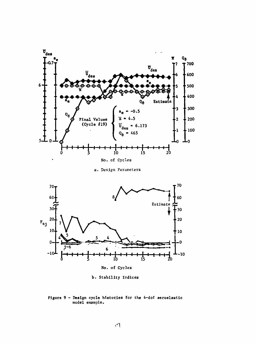
treated as a design parameter, together with EDES and a . e Figure 9 shows the design cycle history for the 4-degree-of-f reedom

The initial objec-

= 4.0 and 5.0 using Q, and CDEs as wing configuration, which includes rigid-body pitch.

tive was to stabilize the system at

design variables. Note that,the closed-loop system is stable at

U = 6.0.

ficulty meeting its objectives. At this point, the position of the

wing, with respect to the pivot, by, was allowed to change, together

with ae, for the next two iterations.

fixed and optimization continued using

- By design cycle number 7, the procedure was experiencing dif-

After cycle 9, a and x were held e

and Q, as design variables. DES

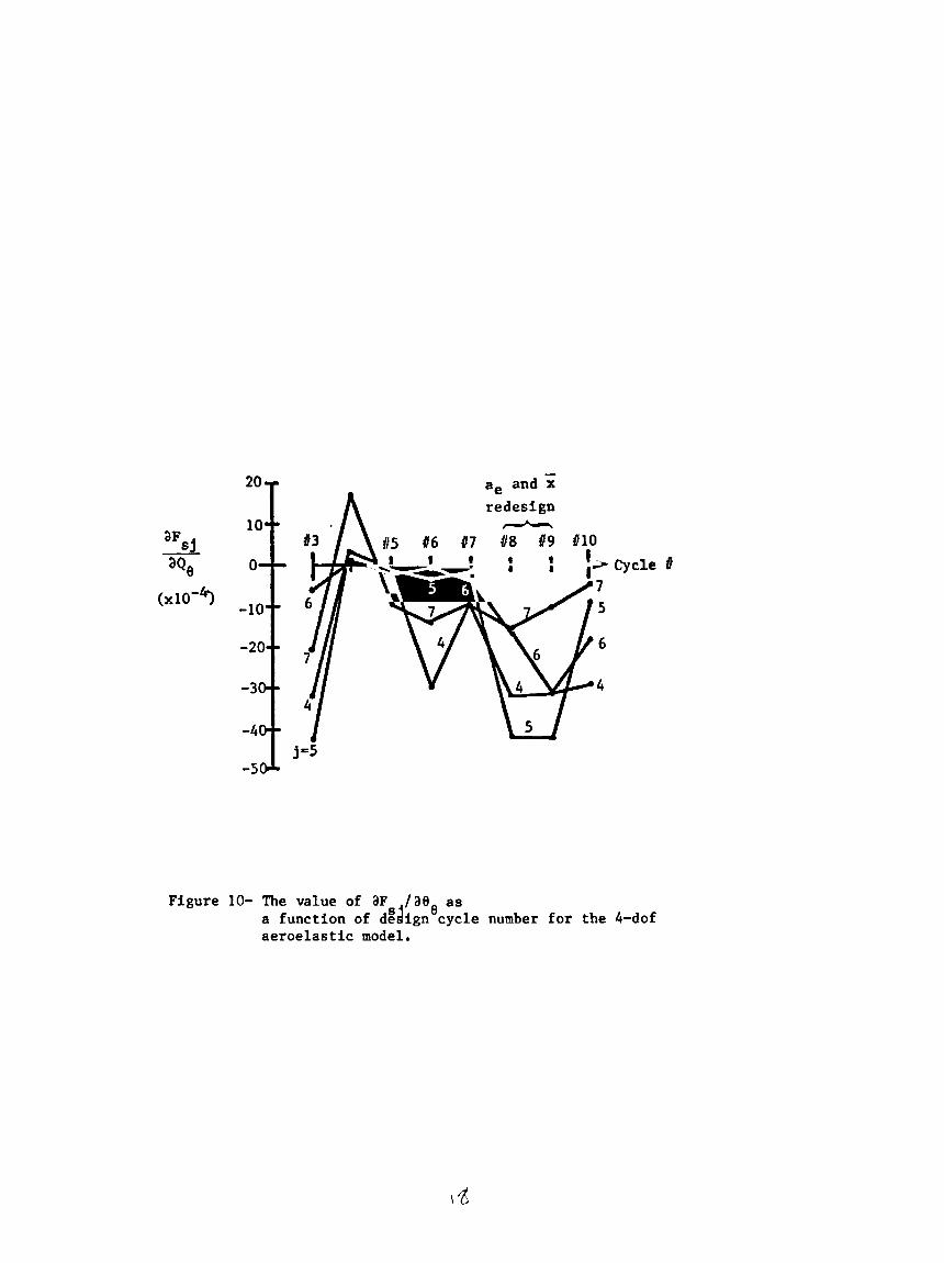
The effects of the use of b; and a as parameters can be seen in e Figure 10. Figure 10 plots the partial derivatives of the stability

indices, with respect to Q,, as functions of design cycle number.

figure indicates that changes in by and a

This

increase the lnagnitudes ox' e

8

these derivatives. As a result, Q, becomes more effective as a design

parameter.

Figure 11 shows the root-locus plots, with 5 as a gain, for the

initial closed-loop design and the final closed-loop design.

design is Been to be a compromtse between flutter at F = 7.04 and

flutter in a hump mode at around 5 - 5.0.

increase the 5 = 7.04 flutter speed, the stability constraint at

The final

If one were to try to further

= 5.0

would be violated.

The paper will describe additional features of this integrated

design technique. Included will be additional data indicating why

several of the features observed in the previous figures occur as they

do, In addition, a discussion will be included as to how this procedure

may be expanded to include control synthesis by techniques other than

SSLQR theory . References

1. Sobieszczanski-Sobieski, J., James, B., and Dovi, A., "Siructural Optimization by Fiultilevel Decomposition," AIAA/kSME/ASCE/AHS 24th Structures, Structural Dynamics and Materials Conference Proceedings, A I A A paper no. 83-0832-CP, Flay 2-4, 1963.

Gilbert, M.G., "Optimal Linear Coatrol Law Design Using Optimum Parameter Sensitivity Analysis,'' Proposal for Doctoral Dissertation F.esearch, Purdue University, School of Aeronautics and Astronautics, 1983.

2.

f

-7 2 + G I -

. %

c

4

0

i

u a

0

0) 4

v! 0

4

0

d

0 I

"3 0

I

r-l

0 1

f 3 I

In 0 I

a 0 I

m 0 I

A AI

.

0

c

JJ Open-Laop / '10

\ /

.

= 5

4

E'

-. 0 . - I I I I - - - I

-0.6 -0 -5 -0.4 -0.3 -0.2 -0.1 0

a e

Figure 6 - Open and closed-loop stability boundaries as a function of a for the 3-dof aeroelastic model; controf laws are synthesized at u = 6.0 DES

53 1.

m 01 4 U A u W 0

0 z

. Q

. P

A U d rl

I I-

01 L 3 M d f4

Figure 8 - Velocity root l o c i , design cyc le # l l for the 3-dof aeroe las t i c model.

'del . -

ii 5

.

x

'des

0 5 10 15 20

F i n a l Values

No. of Cycles

a. Design Parameters

Q0 700

600

No. of Cycles

b . S t a b i l i t y Indices

Figure 9 - Design cycle h i s t o r i e s for the 4-dof a e r o e l a s t i c model example.

20 - redesign -

115 #6 #7 US #9 #lo - aFs j

(xlO'4)

j =5 -5-

Figure 10- The value of aF /ae, as a function of d&gn cycle number for the 4-dof aeroelastic model.

"9 d l I

d --

'I I

i:

APPENDIX B

The attached document summarizes the development of a two-degree

of freedom idealization used to study the interaction between

directional stiffness and feedback control.

by Professor Weisshaar and has been implemented on the computer by

Mr. Sallee. A two-mode flexible model could also be used. However,

past experience with the semi-rigid model has been quite good. As a

result, it is the choice for demonstration purposes.

This model was developed

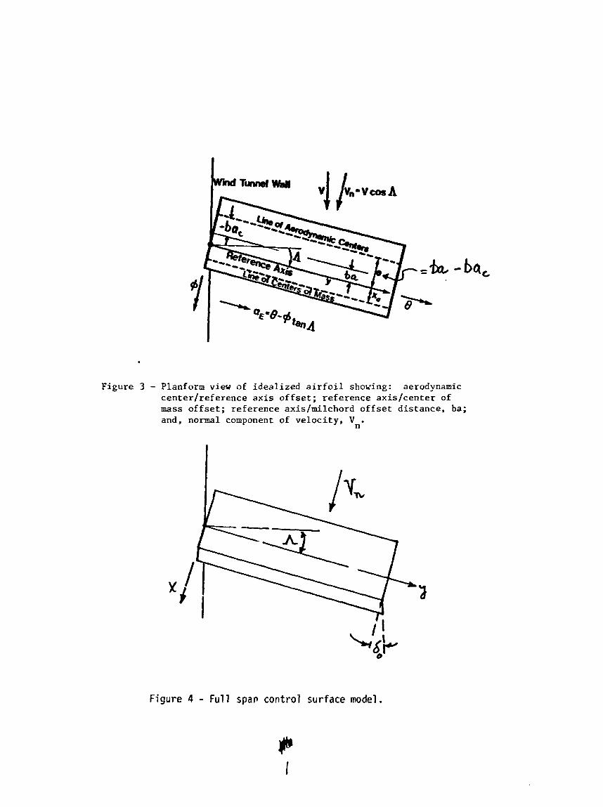
An Idea l ized Aeroelastic Model f o r Active Control S tudies --- -- Consider t h e idea l ized l i f t i n g sur face shorn i n Figures 1, 2, 3.

The su r face I t s e l f is r i g i d , but is a t tached to a pivot on a wall; it

has m s s uniformly d i s t r i b u t e d along the span. A reference a d s , t h e

y-axis in Figure 2, is used f o r t h e determinat ion of the equat ions of

motfon: t he re ference axis lies a d i s t ance ba aft of the midchord. The

l i n e of aerodynamic cen te r s is loca ted a t a d i s t ance ba

a i r f o i l midchord and is shown i n Figure 3.

ahead of the C

For the pos i t i on shown,

b(a-ac) i s a negat ive quant i ty .

c e n t e r s of mass from the re ference a x i s is denoted as x t h i s latter

The chordwise o f f s e t of t he l i n e of

a'

coordinate is pos i t i ve when the sec t iona l cen te r s of mass are located

a f t .of the re ference 2xis.

The downward de f l ec t ion of t he l i n e of cen te r s of mass is denoted . as 2. This d e f l e c t i o n and the ve loc i ty z are expressed i n terms of the

t o r s i o n a l r o t a t i o n , 9, and "bending" r o t a t i o n , +, as:

. . g = ; = Xa9 - $y

The a i r f o i l has constant mass per u n i t l ength , m, so t h a t the k i n e t i c

energy, T, may be wr i t ten as:

o r

1 T = - 2

where Io I s t he p i t c h

1 ' 2 1 1 '2 T = {Ioe 11 f 7 1 mz dy 0

mass moment of Inertia per u n i t length of each

(4)

sec t ion along the wing surface, taken about the l i n e of cen te r s of mass.

The s t r a i n energy i n the spr ing supports due to deformations e and 9 is:

/

/ Figure 1 - Idealized airfoil, shom swept at an angle A to the airstream

and attached to a pivot on the wind-tunnel w a l l .

Figure 2 - Planform view of 2-D, idealized airfoil showing: rotational deformations 8 and $; orientation of principal bending and torsion axes, a; and, effective root and tip approximations.

Figure 3 - Planform view of ideal ized a i r f o i l showing: aerodynamic center lreference a x i s o f f s e t ; reference axis /center of mass o f f s e t ; reference axis/milchord o f f s e t distance. ba; and. normal component of v e l o c i t y , V . n

Figure 4 - Full spar, control surface model.

2

U - 1

Prom Iagrange's equations + T

(5) 2 K { e cos y - + sin y) f e 2 K { + COS y + 8 sin y) +

the equations of motion for free vibration in

the absence of airloads are found to be:

To simplify the writing of these equations, elements of the matrices in

Eqn. 6 are defined as follows.

Inertia terms

m = &x:+ 21 = m&t h e r e r2 = - IO 11 o m

mI2 -- -m 4 {- x$,

(Note that .fl is the total mass of the idealized wing.)

Stiffness terms

kI2 = (KO - Ke)cosy siny

k22 = Kesin 2 Y + K cos 2 y 4

Aerodynamic Forces

Aerodynamic. forces due to the motion of the idealized airfoil, can

be related to the two degrees of freedom, 8 and $. For the present

analysis these forces were computed from modified aerodynamic strip

theory as outlined by Yates in Reference 1.

the y-axis in Figure 3 is denoted as Me, while bending moment about the

The pitching moment about

3

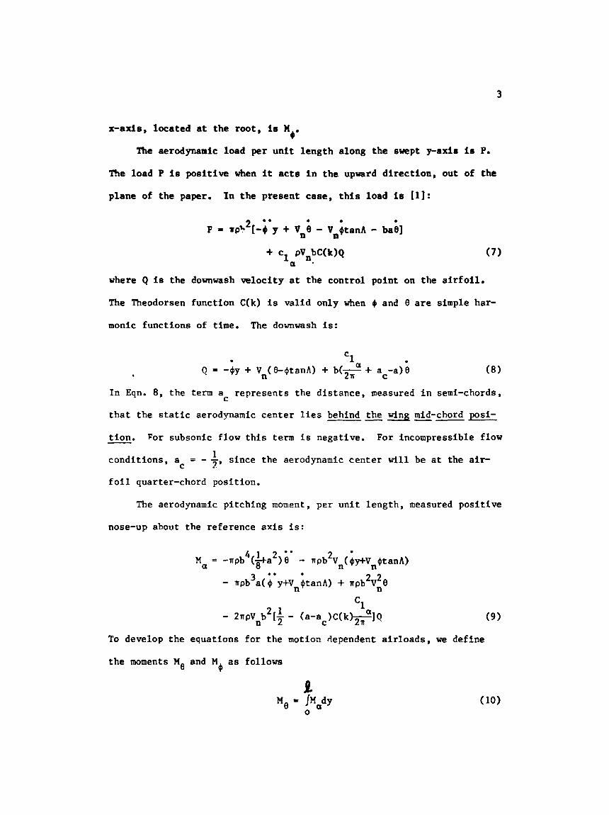
0' x-axis, loca ted a t the root, is M

The aerodynamic load per u n i t l eng th along the swept y-axis its P.

me load P is p o s i t i v e when it acts i n the upward d i r e c t i o n , out of t he

plane of the paper. In t h e present case, t h i s load is [ l ] :

2 -. a . . P = WP? [ - 0 y + Vne - Vn+tanA - bae]

where Q IB the downwash ve loc i ty a t the con t ro l point on the a i r f o i l .

The Theodorsen func t ion C(k) is va l id only when 41 and 8 are simple har-

monic func t ions of time. The downwash is:

I n Eqn. 8 , t he term a r ep resen t s t he d i s t ance , measured i n semi-chords,

t h a t the s ta t ic aerodynamic c e n t e r l i e s behind the wing -- mid-chord posi- C

- - t i on . For subsonic flow t h i s term is negative. For incompressible flow

condi t ions , a = - - s ince the aerodynamic c e n t e r w i l l be a t the air- C 3.'

f o i l quarter-chord posi t ion.

The aerodynamic p i tch ing moment, per u n i t l eng th , measured p o s i t i v e

nose-up about the re ference a x i s is:

Ma = -npb4(3a2)e ' - rpb 2 - Vn(+y+Vn$tanA)

. - rpb 3 a (+ * * y+Vn$tanA) + apb 2 2 Vn8

- 2rpVnb2t+ - (a-a C )C(k)$]Q c1

( 9 )

To develop the equat ions f o r the motion dependent a i r l o a d s , we def ine

t h e moments Me and M as follows 4I

Equations 10 and 11 can be wri t t en as

(12)

I n Eqn. 12, o is a re ference frequency. When motion of the form P

i s assumed, expressions for h, and can be constructed. These expres- d s ions are wr i t t en symbolically as follows:

Elements of the [M

f o i l , while the [B

is the aerodynamic s t i f f n e s s matrix.

] matrix a r e the apparent mass terms f o r t h i s air-

] matr ix represents t he aerodynamic damping. i j

i j [Aij]

The elements of t hese th ree

mat r ices may be conveniently defined i n terms of a group of parameters.

These parameters are:

-2 d = wa

( A R ) * s t r u c t u r a l aspect r a t i o 1/2b

5

The matrix elements are then written as follows:

4(AR)' '22 * 3d

CLc % *11=- md

CL(AR) vn BI2 = ( ( A R ) + a tanh - II 1

- 4 "n B22 = (AR)(tanh + 7 cla (AR)C(k));i-

L

If

-2 cL 'n

*I1 =r f (-1 + -)

-2 CLtanh 1 'n

A12 -2- - (tanh - II

-2

( c1 ( AR) C(k) tanh) '* A22 = nd

a

The equations of motion are written as

1s 2 tmijl + ~ k i j ~ ~ ~ + rnlriwf#J= 0

2 2 a P

Dividing by the factor mlr w gives the following equations:

(22)

(23)

(27 )

(28)

The parameter

- xa - xa/b

while

and

= K11'K22

These matrix equations may be combined and written as

where

[%I = bij1 + [Mijl

[%I = [kijl + [AjJ

This equation may also be written as follows:

the problem in the following form:

If the vector {rl) is defined as

7

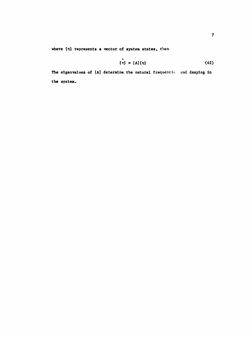
where {n} represents a vector of system states, then

The eigenvalues of [A] determine the natural frequencic and damping in

the system.

8

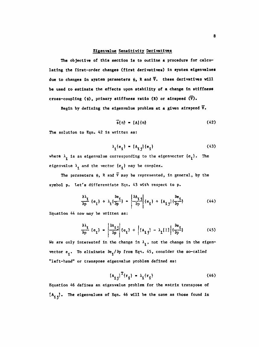
Eigenvalue S e n s i t i v i t y Derivatives

The objec t ive of t h i s s ec t ion is t o o u t l i n e a procedure f o r calcu-

l a t i n g the f i r s t - o r d e r changes ( f i r s t de r iva t ives ) i n system eigenvalues

due to changes i n system parameters e , R and v. t hese de r iva t ives w i l l

be used t o estimate the e f f e c t s upon s t a b i l i t y of a change i n s t i f f n e s s

cross-coupling ($), pr imary s t i f f n e s s r a t i o (R) or a i rspeed (v>. Begin by def in ing the eigenvalue problem a t a given a i r speed 7.

- s { d - [Al{n)

The so lu t ion to Eqn. 42 is wr i t t en as:

XiIeil = [Aijl{ei) (43)

where X

eigenvalue X

i s an eigenvalue corresponding t o the eigenvector {ei). The 1

and the vector {et) may be complex. 1

The parameters $, R and 7 may be represented, i n genera l , by the

symbol p. Le t ' s d i f f e r e n t i a t e Eqn. 43 with respect t o p.

Equation 44 now may be wr i t ten as:

We a r e only i n t e r e s t e d i n the change i n Xi , not the change i n the eigen-

vec tor e

"left-hand" o r t ranspose eigenvalue problem defined as:

To e l imina te ae,/ap from Eqq. 45, consider t he so-called I'

( 4 6 ) T [Aij] {r,) = a i { r i ~

Equation 46 def ines an eigenvalue problem f o r the matrix t ranspose of

[Aij]. The eigenvalues of Eqn. 46 w i l l be the same as those found i n

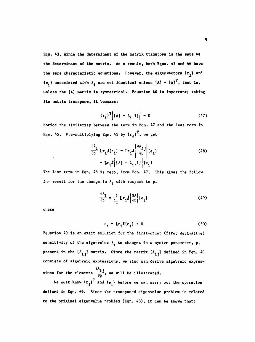
9

Eqn. 43, since the determinant of the matrix t ranspose 1s t he same as

the determinant of the matrix. As a r e s u l t , both Eqns. 43 and 46 have

t h e same c h a r a c t e r i s t i c equations.

(e,) assoc ia ted wlth Xi are _I not i d e n t i c a l un less [A] = [AIT , t h a t is,

unless the [A] matrix i s symmetrical. Equation 46 i s important; taking

its matrix t ranspose, i t becomes:

However, the eigenvectors {ri} and

Notice the s i m i l a r i t y between the term i n Eqn. 47 and the l a s t term i n

Eqn. 45 . Pre-multiplying Eqn. 45 by { r i lT , we g e t

I

The las t term i n Eqn. 48 i s zero, from Eqn. 47. This gives the follow-

inr: r e s u l t f o r the change i n X with respect t o p. 1

where

c i - triJ{eiI + 0

Equation 49 i s an exact so lu t ion f o r t he f i r s t - o r d e r ( f i r s t de r iva t ive )

( 5 0 )

s e u s i t i v i t y of t he eigenvalue X

present i n the [ A ] matrix. Since the mat r ix [ A I def ined i n Eqn. 40

c o n s i s t s of a lgeb ra i c expressions, we a l s o can de r ive a lgeb ra i c expres-

t o changes i n a system parameter, p, 1

ij i j

aA 8iOnS f o r the elements A, as w i l l be i l l u s t r a t e d .

aP T We must know { r 1 and {ei) before we can c a r r y

def ined i n Eqn. 49. Since the transposed eigenvalue

1

t o the o r i g i n a l eigenvalue nroblem (Eqn. 4 3 ) , it can

out the operat ion

problem i s re l a t ed

be shown tha t :

10

[ R l - [El" (51)

where the columns of the NxN modal matr ix [E] are constructed by i nee r t -

i ng the N eigenvectors {ei} such t h a t

As a r e s u l t ,

b

and

Since the node shapes (eigenvectors) of both problems are ort..ogona t o

each o t h e r , the s e n s i t i v i t i e s of a l l eigenvalues can be computed i n a

s i n g l e opera t ion , as follows.

L e t us def ine a matrix [ D ] a s follows: i j

Then

(56) a

= Dii - aP

Note t h a t t he off-diagonal elements of D are not zero, nor are they

meaningful. i j

11

The procedure for computing s e n s i t i v i t y d e r i v a t i v e s of o m eigen-

values is now e a s i l y constructed.

1. Compute t h e N eigenvalues and e igenvec tors of the problem

2. Construct t he matrix [E 1 ij

i j i j 3. I n v e r t [E ] t o f ind [R ]

4. Construct the matrix 121 -3r t h e parameter o i n t e r e s t .

5 . ,Compute [ D ] = [R] 53

a xi Dii 6. -E

aP Now, le t ' s tu rn t o the a c t u a l computation of the mat r ix 121 f a r a few

parameters. F i r s t consider t he s t i f f n e s s cross-coupling parameter JI.

The element

Theref o r e

Next, consider changes with respect t o the primary s t i f f n e s s r a t i o , R =

12

K11’K22’

The element8

Therefore :

of [a are:

r

L

2\ lii: 1 -1 /R (61)

I t i s a l s o important t o predict how the eigenvalues change with

airspeed s ince the eigenvalues determine systen s t a b i l i t y .

pute [+I, a s follows:

Let’s com-

and

[Sj avn

L e t us represent t h e matrix of

1 .. 0 0

J - yr as

changes In

13

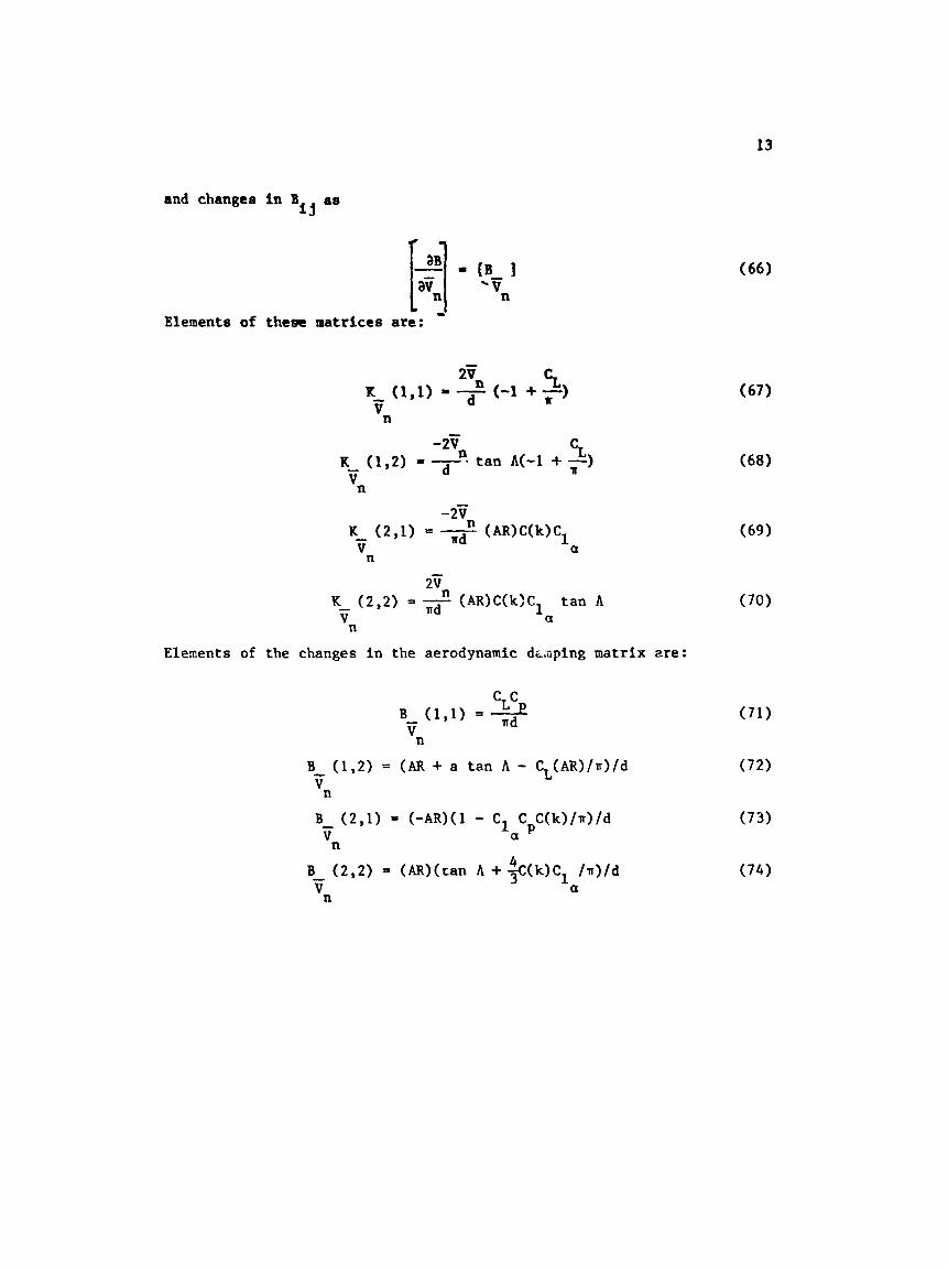
and change6 in B as t j

L ,I Elements of thewe matrices are:

CL 2Tn K, (1,l) = d (-1 + -) 1

'n

Elements of the changes in the aerodynamic daping matrix are:

'n B-(1,2) = (AR + a tan A - CL(AR)/r)/d vn

14

- The -Mdition -- of a Control Surface t o the I d e a l i z a t i o n

I f a ful l -span, t r a i l i n g edge cont ro l is at tached as shown in pig-

If the con- ure 4 , t h e equations of moticn (Eqn. 36) wi l l be modified.

t r o l d e f l e c t i o n is denoted as 60 and t h e cont ro l is i r r e v e r s i b l e , then

p i t ch ing and bending moments a t the a i r f o i l roo t may be wri t ten as:

where

and

Equation 36 now becomes

where

- e r a - a .

C

2vt - + S C ) 2 1 6 C8& = -

fur,, -2

and

(77)

( 7 9 )

In terms of time de r iva t ives of 0 and 9, Eqn. 78 is wri t t en as:

1s

Equation 81 may be wri t t en in state-spacc form as:

where

(83)

Note t h a t t h e symlsl [B] a l s o has been used previously t o denote f o r

aerodynamic damping.

r e f e r t o the con t ro l matrix, i n t h i s case, a vector quant i ty defined in

However, --- i n a l l that fol lows, the symbol B wil l

Eqn. 83.

Modal Cof i t ro l lab l l i ty

The a e r o e l a s t i c response problem is now cast i n terms of the state

vec tor {n) (defined i n Eqn, 4 1 ) as follows:

0

q = A q + B 6 . Again, the eigenvectors of the problem rl = AII are {e,) and, as before ,

can be arranged t o form an NxN modal matrix [E def ined i n Eqn. 51. i j

We can use [E

n a t e s { E , ) , defined as:

] t o transform the n coordinates t o a new s e t of coordl- i j

so t h a t

{ C ) = [Eijl-'{n? = I R l l n ?

Our equat ion of motion, including the con t ro l , then becomes:

16

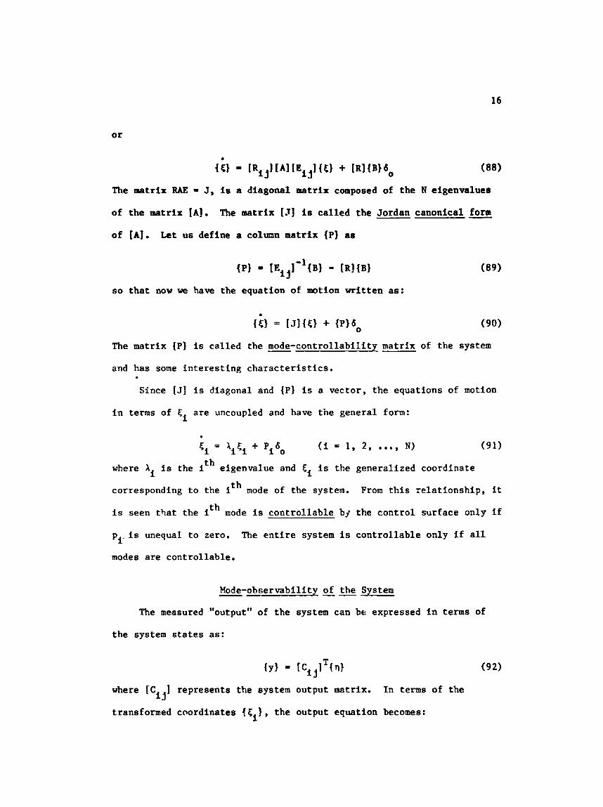
or

The matrix RAE = J, is a diagonal matrix composed of the N eigenvalues

of the matrix [A]. The matrix [.I] is called the Jordan canonical form

of [A]. Let us define a column matrix {P}

so that now we have the equation of motion

.

as

written as:

( 8 9 )

{ E } = [Jl{C} + {P}60 (90)

The matrix {PI is called the mode-controllability matrix of the system

and has some interesting characteristics.

Since [J] is diagonal and {P) is a vector, the equations of motion

in terms of 5 are uncoupled and have the general form: i

5, = \$Ei + Pido (i = 1, 2 , ..., N) (91)

where X is the ith eigenvalue and 5 i i

corresponding to the ith mode of the system. From this relationship, it

is seen that the ith mode is controllable bj the control surface only if

p is unequal to zero.

modes are controllable.

is the generalized coordinate

The entire system is controllable only if all i.

Mode-observability -- of the System - The measured "output" of the system can be expressed in terms of

the system states as:

where [C 1 represents the system output matrix. In terms of the

transformed coordinates {Ei}, the output equation becomes: ij

17

(93)

where

[TI - [EI, lTICI (94)

The matrix [TI i r : called the mode-observabillty matrix for the system.

18

Modal Control

Only a s i n g l e c o n t r o l i npu t , b,, c o n t r o l s t h e aerrelastic system;

let's measure the system states and feedback a signal, f , defined as:

f(t) - {VIT{?) (95)

The matrix {v } is a matrix of t ransducer ou tpu t s from each state.

vec tor {v} is c a l l e d t h e measurement vector.

amplified by a propor t iona l c o n t r o l l e r having a gain, K.

t h e c o n t r o l l e r is 4 so t h a t we move t h e c o n t r o l su r f ace an amount:

This

The signal f(t) can be

I n t h i s case,

O S

Combining t h i s with our equation of motion, we now have t h e following

prohl em.

Let

Then

Depending upon the choice of K and { p )

d i f f e r from those of t he o r i g i n a l p l an t matrix [ A ] . How one chooses K

the eigenvalues of [A,,J w i l l

and {p} depends upon the ob jec t ive of t he con t ro l . L e t u s suppose t h a t

t h e objec t ive is t o modify a s i n g l e eigenvalue of t he o r i g i n a l p lan t .

Let us have as our ob jec t ive the changing of t he jth eigenvalue,

X

open-loop system unchanged. Here is one way t h a t t h i s may be done.

t o a value y while leav ing a l l o t h e r va lues of Xi (i f j) of the j' j

(Note t h a t what follows i s a g r e a t l y s impl i f i ed approach t o a e r o e l a s t i c

19

control . ) Let {u} = {rj) , the jth eigenvector of the transposed eigenvalue

problem. In this case

Now, post-multiply by the kth eigenvector (k f j) of the open-loop sys-

tem, {ek}, to get:

[+I = [AI {e$ + K W I r jlT{ek} (102) T Because of eigenvector orthogonality, {r } {e,} = 0. This leaves J

[\]{e,} = LAIlek} (103)

Since, by definition, [A]{e,} = \{ek}, Eqn. 103 becomes:

[\J{ekl x{e,l (k f j) (104)

This last result in Eqn. 104 means that, for this selection of { p } , the

eigenvectors and eigenvalues of the closed-loop system (represented by

A$ are identical to those of the uncontrolled, open loop system [A],

-- with the exception -- of the jth eigenvalue/eigenvector combination.

look at this latter combination.

Let’s

If we now post-multiply Eqn. 101 by {e 1 then j

[%]lej) = [Al{ej} + K{B}{rj}Tlej}

or

[$]{ej} = [Al{ej} + K(B1 = AjIej} + K@} (106)

Equation 106 is valid because of orthonormality of the vectors {r } and

{e } in Eqn. 105. This result implies that, due to feedback control, X

is not an eigenvalile of [A$, nor is (e } an eigenvector of [\,ID

9

1 9

1

20

Since the vector {u} has been s p e c i f i e d , t h e only unknown i n the

c o n t r o l l a w is K, t he gain. To determine t h e value of K necessary t o

modify Xi by a certain amount, first remember t h a t p

t h e c o n t r o l l a b i l i t y mat r ix for t h e jth mode.

ach ieve our ob jec t ive of eigenvalue modi f ica t ion , we can set the ga in K

t o be:

i s the element of j

It can be shown t h a t , t o

K = ( p j - aj) /pj (107)

t h where p is the element of t h e c o n t r o l l a b i l i t y mat r ix r e l a t e d t o the j

mode and p is the new eigenvalue. Notice t h a t t he ga in K may be com-

plex. This modification procedure i s s t r i c t l y v a l i d only when changing

a real eigenvalue X to a r e a l value p

add an add i t iona l s tep .

j

j

If Xi is complex, w e need t o . j j'