INTERACTIVE METHOD FOR ESTIMATING HAILSTONE … · 0AN INTERACTIVE METHOD FOR ESTIMATING HAILSTONE...

SFILE OP i1I00

0AN INTERACTIVE METHOD FOR ESTIMATING HAILSTONE SIZE

AND CONVECTIVELY-DRIVEN WIND GUSTS FROM

FORECAST SOUNDINGS

OTICS ELECTE *

FEB 2 3 1990 U

D

John Philip Pino, B.S.

A ppz~u'v d L~i puHtlc: r 1_

_,Dtmu on Uiniu~ d[

D

A Digest Presented to the Faculty of the Graduate

School of Saint Louis University in Partial

Fulfillment of the Requirements for the

Degree of Master of Science (Research)

1989

90 02 21 058

SF.CURITY CLASSIFICATION O THIS PAGE

Form ApprovedREPORT DOCUMENTATION PAGE MB No. 0704-0188

la. REPORT SECURITY CLASSIFICATION lb. RESTRICTIVE MARKINGSUNCLASSIFIED NONE

2a. SECURITY CLASSIFICATION AUTHORITY 3. DISTRIBUTION /AVAILABILITY OF REPORTAPPROVED FOR PUBLIC RELEASE;

2b. DECLASSIFICATION /DOWNGRADING SCHEDULE DISTRIBUTION UNLIMITED.

4. PERFORMING ORGANIZATION REPORT NUMBER(S) 5. MONITORING ORGANIZATION REPORT NUMBER(S)

AFIT/CI/CIA- 89-048

6a. NAME OF PERFORMING ORGANIZATION 6b. OFFICE SYMBOL 7a. NAME OF MONITORING ORGANIZATIONAFIT STUDENT AT SAINT (If applicable) AFIT/CIA

LOUIS LUNIVERSITY6c. ADDRESS (City, State, and ZIP Code) 7b. ADDRESS (City, State, and ZIP Code)

Wright-Patterson AFB OH 45433-6583

8a. NAME OF FUNDING/SPONSORING 8b. OFFICE SYMBOL 9. PROCUREMENT INSTRUMENT IDENTIFICATION NUMBERORGANIZATION (If applicable)

8c. ADDRESS (City, State, and ZIP Code) 10. SOURCE OF FUNDING NUMBERS

PROGRAM PROJECT TASK WORK UNITELEMENT NO. NO. NO ACCESSION NO.

11. TITLE (Include Security Classification) (UNCLASSIFIED)An Interactive Method for Estimating Hailstone Size and Convectively-Driven Wind GustsFrom Forecast Soundings

12. PERSONAL AUTHOR(S)John Philip Pino

13a. TYPE OF REPORT 13b. TIME COVERED 114. DATE F REPORT (Year, Month, Day) 15. PAGE COUNTTEIW R MFROM TO I 1989 1 98

16. SUPPLEMENTARY NOTATION APPROVE13 k-UR PUBLIC RELEASE IAW AFR 190-1ERNEST A. HAYGOOD, 1st Lt, USAFExecutive Officer, Civilian Institution Programs

17. COSATI CODES 18. SUBJECT TERMS (Continue on reverse if necessary and identify by block number)

FIELD GROUP SUB-GROUP

19. ABSTRACT (Continue on reverse if necessary and identify by block number)

20. DISTRIBUTION /AVAILABILITY OF ABSTRACT 21. ABSTRACT SECURITY CLASSIFICATIONMUNCLASSIFIED/UNLIMITED 0 SAME AS RPT. C DTIC USERS UNCLASSIFIED

22a. NAME OF RESPONSIBLE INDIVIDUAL 22b. TELEPHONE (Include Area Code) 22c. OFFICE SYMBOLERNEST A. HAYGOOD, 1st Lt, USAF (513) 255-2259 AFIT/CI

DO Form 1473, JUN 86 Previous editions are obsolete. SECURITY CLASSIFICATION OF THIS PAGE

AFIT/CI "OVERPRINT"

DIGEST

Interactive methods for forecasting potential

hailstone size and convectively-driven surface wind

gust velocities are applied to forecast soundings

which better represent atmospheric conditions prior

to the onset of convection. The forecast sounding

is based upon the 1200 UTC sounding and is developed

interactively by the user considering diurnal

changes expected to occur in the lower tropospheric

levels over the next 6-12 hours. Changes to the

middle and upper levels are estimated by taking a

fraction of the mean geostrophic advection of

temperature for consecutive layers and adjusting the

1200 UTC sounding accordingly. Interactive

capability allows for final adjustment of any or all

of the data. Hailstone size and convectively-driven

wind gusts are based upon key thermodynamic

parameters (e.g., CCL, LFC, CAPE) derived from the

forecast sounding. -

Hailstone size is determined using three

separate routines. The first is based upon

techniques described in AWS TR-200 which is a0

function of the CCL and is used extensively by the

USAF Air Weather Service. The other two methods

relate the hailstone size to its terminal velocity

odes

VDist xcaSAi Clal

Alt

2

which in turn is a function of the maximum expected

updraft in the cloud. For these methods, an

algorithm considers the role of heat transfer from

the environment to the hailstone during the stone's

descent to account for melting.

Convectively-driven surface wind gusts are

estimated three ways. One method automates a

technique described in AWS TR-200. In the second

method, the wind gust is a function of the

temperature of a parcel brought down from the Level

of Free Sink (LFS) moist-adiabatically to the

surface and the surface environmental temperature.

A third method integrates Anthes' vertical motion

equation downward from the LFS to the surface.

Hail and strong wind proximity soundings from

AVE-SESAME I and II and OK PRE-STORM were used to

validate the procedures. For 58 cases studied, the

Pino-Moore hail method resulted in a Student-t

statistic significant at the 0.596 level compared

with a 10% level for the AWS TR-200 technique. The

forecast sounding algorithm produced a mean diameter

error of +0.03 cm compared to -1.18 cm for 15

proximity soundings. Validation of the three wind

gust methods resulted in little discriminatory skill

but the bias and scatter scores did favor Anthes

method as more operationally suitable.

AN INTERACTIVE METHOD FOR ESTIMATING HAILSTONE SIZE

AND CONVECTIVELY-DRIVEN WIND GUSTS FROM

FORECAST SOUNDINGS

John Philip Pino, B.S.

A Thesis Presented to the Faculty of the GraduateSchool of Saint Louis University in PartialFulfillment of the Requirements for theDegree of Master of Science (Research)

1989

COMMITTEE IN CHARGE OF CANDIDACY

Associate Professor James T. Moore,

Chairperson and Advisor

Professor Yeong-Jer Lin

Professor Gandikota V. Rao

ACKNOWLEDGEMENTS

My deepest appreciation is extended to Dr James

Moore for his guidance and technical support

throughout my research. I would also like to offer

gratitude to Professors Rao and Lin for their expert

advice. Also, the Air Weather Service of the United

States Air Force for offering me the opportunity to

attend graduate school.

I cannot complete my acknowledgements without

mentioning the spiritual support and understanding I

received from my wife, Elaine. Her patience and

encouragement on countless occasions enabled me to

complete this degree.

ii

TABLE OF CONTENTS

Chapter 1. Introduction to the Problem ..... 1

Chapter 2. Review of Related Literature .... 5

2.1 Forecasting Hailstone Size ......... 5

2.2 Estimating Convectively-Driven WindGusts ............................. 14

2.3 The Forecast Sounding ..... ........... 16

Chapter 3. The Procedure ..... ................. 18

3.1 Hail Size Formulation ..... ........... 18

3.1.1 Calculating the VerticalUpdraft ...... ................. 18

3.1.2 Drag Coefficient andHailstone Density .............. 23

3.1.3 Hailstone Melting ..... ......... 24

3.2 Estimating Convective Wind Gusts .. 30

3.3 The Forecast Sounding Algorithm ... 31

3.3.1 Diurnal Changes ..... ........... 31

3.3.2 Middle and Upper LevelChanges ...... ................. 35

3.4 Validation Procedures ..... ........... 36

3.5 The Sounding Analysis Package ..... 40

Chapter 4. Results and Discussion .............. 42

4.1 Hail Size Forecast Validation ..... 44

4.1.1 Combined Cases ..... ............ 44

4.1.2 Composite Soundings ........ 50

4.2 Convective Wind Gust Validation ... 56

4.3 Sensitivity Study of Key Variables 60

4.4 Forecast Sounding Utility ......... 62

iii

4.4.1 Limitations and Weaknesses 66

4.5 Case Study ...... ..................... 68

Chapter 5. Summary and Conclusions ............ 83

5.1 Research Summary ..... ................ 83

5.2 Future Considerations ................ 86

APPENDIX .................................... 88

REFERENCES .................................. 95

BIOGRAPHY OF THE AUTHOR ........................ 98

iv

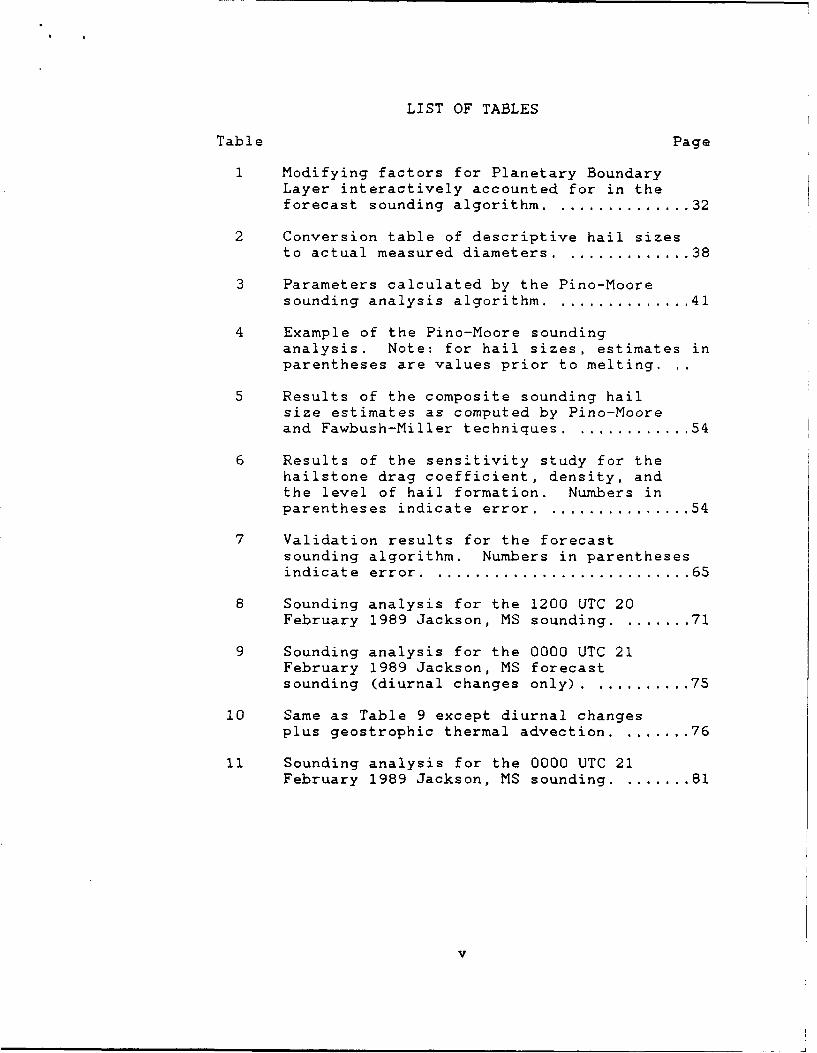
LIST OF TABLES

Table Page

1 Modifying factors for Planetary BoundaryLayer interactively accounted for in theforecast sounding algorithm ................ 32

2 Conversion table of descriptive hail sizesto actual measured diameters ............... 38

3 Parameters calculated by the Pino-Mooresounding analysis algorithm ................ 41

4 Example of the Pino-Moore soundinganalysis. Note: for hail sizes, estimates inparentheses are values prior to melting.

5 Results of the composite sounding hailsize estimates as computed by Pino-Mooreand Fawbush-Miller techniques .............. 54

6 Results of the sensitivity study for thehailstone drag coefficient, density, andthe level of hail formation. Numbers inparentheses indicate error ................. 54

7 Validation results for the forecastsounding algorithm. Numbers in parenthesesindicate error .. ........................... 65

8 Sounding analysis for the 1200 UTC 20February 1989 Jackson, MS sounding ......... 71

9 Sounding analysis for the 0000 UTC 21February 1989 Jackson, MS forecastsounding (diurnal changes only) ............ 75

10 Same as Table 9 except diurnal changesplus geostrophic thermal advection ......... 76

11 Sounding analysis for the 0000 UTC 21February 1989 Jackson, MS sounding ......... 81

V

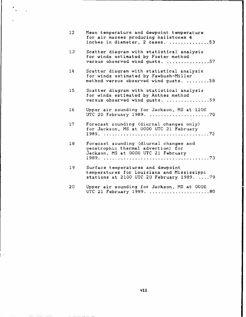
LIST OF FIGURES

Figure Page

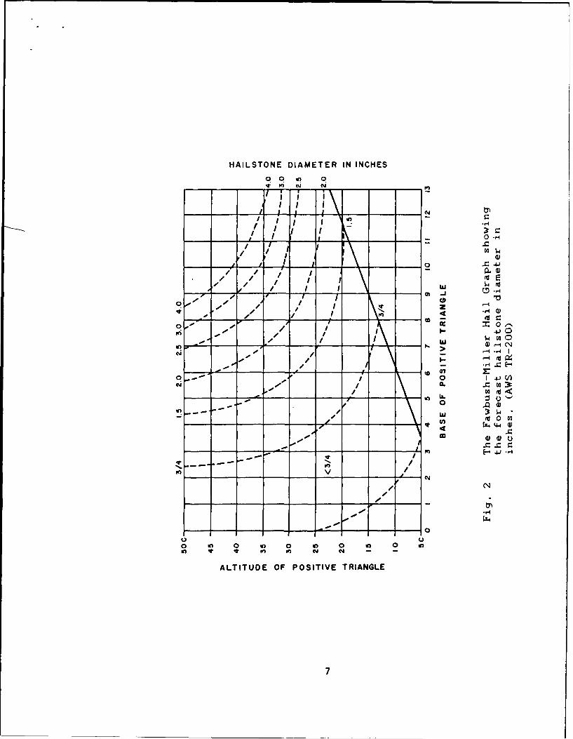
1 Positive area appproximated by Fawbush-Miller technique. BB' is the base of thepositive triangle and HH' measures thealtitude .. .................................. 6

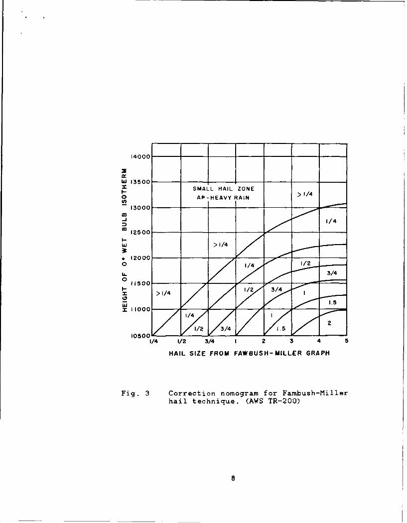
2 The Fawbush-Miller Hail Graph showingthe forecast hailstone diameter ininches .. .................................... 7

3 Correction nomogram for Fambush-Millerhail technique .. ............................ 8

4 Comparison of updraft velocity estimatedfrom balloon ascent rate (solid line)and from parcel buoyancy (dashed line).Height in kilometers MSL ................... 13

5 Example sounding with correspondingpositive and negative areas as computedfrom the LFC and CCL. Dashed lines slantingto the left are dry adiabats, dashed linesslanting to the right are constant mixingratio lines, dashed-dot lines are moistadiabats .. .................................

6 Idealized energy input by surface heating(shaded area is one energy box). Totjlheat realized is 50 boxes ( 350 J kg )At is time from sunrise. E is energyrealized for a given At (in boxes) ......... 34

7 Scatter diagram with statistical analysisfor Pino-Moore hail diameter estimatesversus observed hail diameters ............. 45

8 Scatter diagram with statistical analysisfor Fawbush-Miller hail diameter estimatesversus observed hail diameters ............. 46

9 Scatter diagram with statistical analysisfor Fawbush-Miller hail diameter estimateswithout melting .. .......................... 49

10 Mean temperature and dewpoint temperaturefor air masses producing hailstones 1/2inch in diameter, 68 cases ................. 51

11 Mean temperature and dewpoint temperaturefor air masses producing hailstones 1 inchin diameter, 25 cases .. .................... 52

vi

12 Mean temperature and dewpoint temperaturefor air masses producing hailstones 4inches in diameter, 2 cases ................ 53

13 Scatter diagram with statistical analysisfor winds estimated by Foster methodversus observed wind gusts ................. 57

14 Scatter diagram with statistical analysisfor winds estimated by Fawbush-Millermethod versus observed wind gusts .......... 58

15 Scatter diagram with statistical analysisfor winds estimated by Anthes methodversus observed wind gusts ................. 59

16 Upper air sounding for Jackson, MS at 1200UTC 20 February 1989 .. ..................... 70

17 Forecast sounding (diurnal changes only)for Jackson, MS at 0000 UTC 21 February1989 .. ..................... ....... ..... .... 72

18 Forecast sounding (diurnal changes andgeostrophic thermal advection) forJackson, MS at 0000 UTC 21 February198 9 .. .. ............................... .... 7 3

19 Surface temperatures and dewpointtemperatures for Louisiana and Mississippistations at 2100 UTC 20 February 1989......79

20 Upper air sounding for Jackson, MS at 0000UTC 21 February 1989 .. ..................... 80

vii

1. INTRODUCTION TO THE PROBLEM

During the early 1950's, the Air Weather

Service (AWS) of the United States Air Force

undertook a major study dealing with severe

thunderstorm forecasting. The study was headed by

Lt. Col. Ernest Fawbush and Maj. Robert Miller with

the primary goal of improving AWS's capability for

providing severe thunderstorm support to varied

customers within the Department of Defense (DoD)

along with its numerous missions. The result of

this study, 'Notes On Analysis and Severe-Storm

Forecasting Procedures of the Air Force Global

Weather Central" (AWS Technical Report 200, 1972),

provides techniques for hand calculating potential

hailstone size and convectively-driven surface wind

gust velocities. For the past 35 years. AWS has

issued countless warnings for severe thunderstorms,

many of which included specific user-oriented

information for hailstone size and convectively-

driven surface wind gust velocities derived from the

procedures described in AWS TR-200.

As tiie physical and dynamical understanding of

thunderstorms and their environment evolved during

the past twenty five years, AWS recognized the

2

need and, more importantly, the capability for

improved customer support by considering the

temporal changes of the atmosphere between

rawinsonde sampling times (12 UTC and 00 UTC).

Gesser and Wallace (1986) describe a technique for

forecasting changes for an air mass from its

sampling time at 12 UTC to the estimated time of

convective development, usually some 6 to 12 hours

later.

The Air Weather Service is about to undergo a

complete revolution in its customer support during

the early 1990's with the acquisition of the

Automated Weather Distribution System (AWDS) and the

Next Generation Weather Radar (NEXRAD) . These major

programs possess the capability of automating many

of the day-to-day "routine" tasks forecasters

perform. Consequently, many forecasting techniques,

such as those in AWS TR-200, can now be automated.

Although automating the AWS TR-200 techniques

for forecasting hail size and wind gust velcities is

a logical first step, AWS can now work towards

improving its severe storm support. An advanced

system such as AWDS provides AWS with the capability

of incorporating more sophisticated techniques into

3

its diagnosis and short-term forecasts of the severe

storm environment. A critical part of determining

the atmosphere's potential for severe convection is

the comprehensive diagnosis of the pre-storm

sounding. Additionally, there is a definite need to

develop an automated forecast sounding technique

which would permit interaction with the forecaster

on a "what-if" basis, allowing him to create a

likely thermodynamic profile for 6-12-hours from

1200 UTC. These two steps alone would enhance the

AWS's severe thunderstorm forecasting capability by

exploiting the knowledge gained in this area over

the past 2-3 decades.

The major thrust of this research is to develop

viable, automated methods for forecasting potential

hailstone size and surface wind gusts from

rawindsonde data. These methods will be applied to

objectively-derived forecast soundings which better

represent atmospheric conditions prior to the

development of convection. Diagnostic methods will

be developed, based upon recent developments in

understanding severe convection, which offer a more

complete diagnosis of the morning sounding.

Techniques to produce a 6-12 h forecast sounding

will be discussed and tested on special case studies

4

to evaluate their utility in the operational

environment. Forecast schemes for hail size and

convective wind gust determination will be described

which more fully exploit the thermodynamic profile

at a station. The ultimate goal is to develop

operationally useful diagnostic/prognostic tools

which would improve the forecasting of severe

weather attending strong convection.

2. REVIEW OF RELATED LITERATURE

2.1 FORECASTING HAILSTONE SIZE

The Air Weather Service forecasting techniques

for hail size and maximum wind gusts of convective

origin are described in Chapters 9 and 10,

respectively, of the AWS Technical Report 200. The

technique for forecasting hail size requires the use

of a nomogram (Fig. 1) . Tracing the moist adiabat

from the CCL to the pressure level where the dry-

bulb air temperature is -5 C forms the first side of

a triangle defining the positive area. This

pressure level, the dry-bulb temperature curve, and

the moist adiabat through the CCL form the triangle

representing the positive area. After determining

the base (horizontal coordinate) and altitude

(vertical coordinate) of the positive triangle, a

hailstone diameter of up to four inches can be

interpolated from a nomogram (Fig. 2).

A correction (reduction) based on the height of

the Wet-Bulb-Zero (WBZ) can then be made using the

nomogram shown in Fig. 3. This nomogram requires

the height of the 00 wet bulb isotherm (vertical

coordinate) and the hail size previously determined

(horizontal coordinate) from Fig. 2. This

5

So D 20* D -150 -100 Do 500

x 0

100

S-150 x

ISOBAR WHEREBH B' TEMPERATURE=-50

60C S 101D 150S20 s 25 S 30

aliud.0A0TR20

0 6

HAILSTONE DIAMETER IN INCHES

I J

lo - -

n/ LL .I- -o o

/" / /r I -/ / In

- / , I ~ - w,.

0 0 0 0" ,,/ 2 €

, - _ _! / I I4I' .O)

It in ej W

A OF P T TI

• p I0 Ir (,"

" I~~ IL ,

-- / w

4. .I

o. -- /A--UD F O IIETINn

V7

14000

aJI 13500I- SMALL HAIL ZONE0 AP-HEAVY RAIN>1/

13000

12500 ___

00

I I

4 54

HAIL SIZE FROM FAWBUSH-MILLER GRAPH

Fig. 3 Correction nomogram for Farnbush-Millerhail technique. (AWS TR-200)

8

9

correction is made only for cases where the WBZ

height is above 10,500 feet.

Bilham and Relf (1937) considered a spherical

hailstone of diameter, d. When dropped from rest in

a quiescent atmosphere, the hailstone will

accelerate downward until the aerodynamic drag force

is just equal to the hailstone weight thus reaching

its terminal velocity.

Cd Pa Ph (d3

The left-hand side of (1) is the expression for the

drag of the hailstone where Cd is the drag

coefficient, A is the density of air computed using

the equation of state at the pressure level of hail

formation, and V is the terminal velocity of theh

hailstone. The right hand-side is equal to the

hailstone's weight where A is the density of ice, g

is the acceleration of gravity, and d is the

diameter of the hailstone.

Solving (1) for Vh yields:

2Phgd (2)h - 3 PaCd

10

In (2) Vh can be thought of as the downward

velocity required to make the viscous force equal to

the gravitational force in (1); i.e., no

acceleration takes place. Foster and Bates (1956)

assumed that the environmental upward vertical

velocity required to suspend the hailstone is nearly

equal to this terminal velocity. The updraft within

the thunderstorm provides this necessary

suspension. Their technique for relating the

suspending updraft to hailstone diameter is based qn

the following premises:

1. the updraft velocity prevailing in the zone

of hail formation is the velocity required to just

sustain the fully grown hailstone (i.e., the stone's

terminal velocity),

2. this updraft velocity is derived from the

buoyancy force acting on parcels in the updraft

above the level of free convection (LFC),

3. this velocity (and, therefore, the hail

size) may be calculated from the positive area below

the level of hail formation as determined on a

thermodynamic diagram of a sounding of the air mass

taken very close to the site and time of the hail

occurrence.

ii

Foster and Bates (1956) relate the vertical

accelerations of a non-entraining parcel to the

buoyancy force given by

= g (3)wg( T

where w is the vertical acceleration of a parcel, T'

is the temperature of the parcel, and T is the

temperature of the environment. Upon integration,

1

Wh = (AT, H) 2 (4)TM

where w h is the vertical velocity at the height of

hail formation, T is the mean temperature of them

environment from the LFC through height H, the level

of hail formation, A TH is the difference of the

parcel temperature and the environmental temperature

at the level where the parcel temperature is -100 C

and w at the LFC is assumed to be zero. The

diameter of a potential hailstone can now be

calculated by substituting wh for Vh in (1)

yielding:

2d 3 p. Cd wh

Pd d=W (5)

2 Ph 9

Bluest ein et al . (1988) analyzed soundings

12

obtained by a storm-intercept crew using mobile

sounding units. A sounding was launched into the

wall cloud of a severe storm near Canadian, Texas on

7 May 1986. Neglecting the effects of water loading

and vertical perturbation pressure gradients, a

vertical updraft speed profile was calculated and

compared with the measured updraft speeds (Fig. 4)

In the calculated updraft profile, the vertical

velocity above the LFC at height h is a function of

the convective available potential energy (CAPE).

Bluestein assumed that the parcel's vertical

velocity is near zero at the LFC. Both profiles are

in close agreement between 2.3 and 7.2 km, thus

validating the parcel method of estimating vertical

velocities.

Based on the techniques described by Prosser

and Foster (1966), an effort was undertaken by the

National Severe Storms Forecast Center (NSSFC) to

determine the utility of calculating potential

hailstone size and wind gust velocities from

operational rawindsonde data. Since the hail

algorithm rarely calculated hail potentials greater

than one inch and the wind algorithm resulted in

little discriminatory skill, the authors concluded

that these algorithms be dropped from the NSSFC

9/

//

8-/

7/

/1

11

//

6 //

6 /

5,//

24//

w

3 //

2-

p I I

0 I0 20 30 40 50 60VERTICAL VELOCITY (m 8" )

Fig. 4 Comparison of updraft velocity estimatedfrom balloon ascent rate (solid line)and from parcel buoyancy (dashed line).Height in kilometers MSL. (Bluestein et.al. 1988)

13

14

computerized raob analysis package.

Leftwich (1984) applied Foster and Bates'

technique to assess the predictive potential of

rawindsonde data close in time and space to hail

events. Leftwich considered 12 hail events which

occurred within 100 km and + 2 h of a rawinsonde

sounding. Leftwich (1986) continued this

investigation obtaining hail size estimates based on

VISSR Atmospheric Sounder (VAS) data for 5 hail

events. He concluded that when using representative

airmass soundings, his one-dimensional model

produced encouraging results which favored continued

efforts in developing an operational objective aid

for the Severe Local Storm (SELS) forecast unit

forecaster.

2.2 ESTIMATING CONVECTIVELY-DRIVEN WIND GUSTS

Fawbush and Miller (1954) present a procedure

fo- forecasting peak wind gusts in non-frontal

thunderstorms. This technique is still used today

by the Air Weather Service. Their study revealed a

relationship between peak wind gusts and the

temperature difference between the surface air

underneath and in advance of the thunderstorm. The

15

"downrush" temperature under the thunderstorm is

forecast by lowering the wet-bulb freezing level

temperature to the surface along a saturation

adiabat. The difference between the surface

temperature and the downrush temperature, t, is used

to compute a peak gust according to (6):

Peak Gust = 7+3.06t-O.0073t 2-O.000284t 3 (6)

Foster (1958) integrates the bouyancy equation

to find the downward speed of a parcel of air that

becomes cooler than its environment and sinks to the

ground. He approximates the downrush speed

according to:

WO g ZATo) (7)

where w is the vertical velocity of the parcel at

the surface, Z is the height above ground of the

level where the descending parcel and the

environment have equal temperatures (the level of

free sinking), A T is the difference at the surfaceo

of the environment temperature and the "mid-way

moist adiabat", and T is the mean temperature of

mthe parcel in descent.

16

Foster (1958) as well as Fawbush and Miller

(1954) point out that surface gusts may be

influenced by the speed of the thunderstorm. To

test this possible effect, Foster averaged the winds

at 700 and 500 mb for each of the 100 cases and the

resulting speed was added to the computed downdraft

speed. However, this yielded a correlation

coefficient of 0.51, an improvement of only 0.01

compared to the results without this correction.

2.3 THE FORECAST SOUNDING

Doswell et al. (1982) first conclusion

confirmed the premise that to determine more

accurate hailstone size and wind gust velocities, a

more representative profile of the atmospheric

conditions prior to the onset of convection is

necessary. Gesser and Wallace (1985) offer a useful

but subjective approach in which adjustments to the

12 UTC sounding are determined primarily by

estimating thermal advection at 850, 700, and 500 mb

using standard upper air analyses. Crum and Cahir

(1983) considered using subjective methods along

with numerical guidance to estimate changes in the

environmental profile. The modifications included

upper air changes, vertical exchange simulations,

17

and surface dewpoint changes. These changes were

tested for the subsequent impact in real-time

forecasts of shower-top elevation calculated by the

Anthes (1977) l-d cloud model. Their results

indicated that modification of the sounding,

particularly in the lower levels, produced better

forecast estimates of the shower cloud tops. In

particular, knowledge of the afternoon surface

dewpoints prior to convective development produced

estimates of shower-top elevations better than or

equal to any other modification.

McGinley (1986) offers a method for estimating

the diurnal changes for the lowest 1.5 km of a

sounding by considering explicitly the sensible

warming from the ground. This heating process can

be prominent for dynamically weak situations. This

method is addressed in section 3.3.1.

3. THE PROCEDURE

3.1 HAIL SIZE FORMULATION

3.1.1 CALCULATING THE VERTICAL UPDRAFT

Foster and Bates' technique only considers a

non-entraining buoyancy force in determining the

vertical velocities. A proposed methodology adapts

their technique but employs the vertical velocity

equation from the Anthes (1977) one-dimensional

cloud model,

w2___-_ B _

2 g_____ P_

dz (1+ ) (8)

where w is the vertical velocity, g is gravity,pis

the entrainment rate given by 0.183/R where R is the

radius of the cell (2000 m), OC is the "virtual mass

coefficient" equal to 0.5 which compensates for the

neglect of nonhydrostatic pressure perturbations,

and Qtw is the total liquid water content expressed

as the ratio of the mass of water to the mass of

air. The buoyancy term B is given by

(Tvc-Tve) (9)Tve

where T and T are the virtual temperature of thevc ye

cloud updraft and the environment, respectively.

18

19

The virtual temperature of the cloud updraft is

determined by

TC T'+ (exp(.Az-1))Tve (10)exp(j±Az)

where T/ is the cloud temperature before mixing withc

the environmental air and z is the change of height

between computational levels. The retarding effects

on the parcel's acceleration due to liquid water

drag and entrainment of slow-moving air from outside

the upward-moving parcel are included in the second

and third right-hand side (RHS) terms of (8).

Upon integration, in a pressure coordinate

form, (8) becomes

_( T

_ - v e_(1+ _)_ Tve ) r p

w2 = w2 + 2Rd TveQtw - 2 (11)wUw +2RdZ( 1 (11))1g Pu

In the proposed model, w is calculated using a

boot strap method in increments less than or equal

to 15 mb from both the LFC and the Convective

Condensation Level (CCL) up to the level of hail

formation. Foster and Bates (1956) determined that

the representative level of hail formation is where

the parcel temperature is equal to -10 0 C. Estimates

of the potential hailstone size can then be

20

calculated by substituting the wa's based upon the

positive areas above the LFC and CCL into (5).

Figure 5 depicts the positive and negative

areas defined by the CCL and LFC. The proposed

algorithm first determines the lifting condensation

level (LCL) by computing the average potential

temperature and the average mixing ratio of the

lowest 100 mb of the sounding. This is done by

calculating the potential temperature over a small

layer and multiplying that temperature by the

fraction that that layer is of 100 mb. Whereas the

average potential temperature is computed by a

pressure weighting scheme, the average mixing ratiok

is weighted according to p

Further lifting of the parcel along a moist

adiabat causes the parcel to reach its LFC. Areas 2

and 3 represent the negative areas proportional to

energy. A mechanical lifting process such as

frontal and orographic lifting, or convergence is

required to overcome this negative area in order for

the parcel to reach its LFC. Upon reaching the LFC,

the parcel becomes warmer than the surrounding

environment resulting in the postive area labeled 1

bounded by the moist adiabat and the dry-bulb

EL

700

),

\\ LL

850 C

1000 Tdmix '-

10'vo

Fig. 5 Example sounding with correspondingpositive and negative areas as computedfrom the LFC and CCL. Dashed linesslanting to the left are dry adiabats,dashed lines slanting to the right areconstant mixing ratio lines, dashed-dotlines are moist adiabats.

21

22

temperature curve. This positive area is

proportional to the amount of kinetic energy gained

by the parcel from the environment. The positive

area bounded by the pressure level where the parcel

temperature is -100 C, the dry-bulb curve, and the

moist adiabat represents the energy which is used in

computing the vertical updraft.

In situations where a lifting mechanism is not

available to overcome the negative area, diurnal

heating may supply the necessary energy for

convection to develop. The algorithm determines the

intersection of the dry-bulb curve and the mixing

ratio corresponding to the surface dewpoint

temperature. This intersection defines the parcel's

CCL. Tracing this CCL along a dry adiabat down to

the surface pressure level determines the convective

temperature. Area 4 is the energy needed by diurnal

heating for the parcel to reach its convective

temperature. Lifting the parcel moist adiabatically

from the CCL until the dry-bulb curve is intersected

again defines the other EL based on the CCL. The

positive areas labeled as 1 and 5 are used by the

algorithm to calculate the vertical updraft.

In an operational setting, the forecaster must

23

decide what type of triggering mechanism will

initiate the expected convection. As seen in Fig.

5, the amount of energy available is quite different

depending upon what type of trigger is anticipated.

It is for this reason that the forecaster needs to

be aware of what mechanisms or physical processes

will initiate the convection. If convection due to

diurnal heating is expected, the forecaster would

base his estimate of hailstone size as predicted by

the updraft formed from the energy from areas. 1 and

5, i.e., the CCL approach. If a lifting mechanism

is expected, the forecaster could adjust the hail

size estimate to correspond with the updraft formed

from area 1, i.e., the LFC approach.

3.1.2 DRAG COEFFICIENT AND HAILSTONE DENSITY

Macklin and Ludlam (1961) concluded from their

experiments that a reasonable mean value of the drag

coefficient for large, asymmetrical hailstones

greater than 1 cm in diameter is 0.6. Prosser and

Foster (1966) also incorporated a drag coefficient

of 0.6 in their technique. This value is

considerably lower, 45% lower, than the mean value

of 0.87 given by Matson and Huggins (1980). Matson

and Huggins' value is based on velocity data

24

obtained for about 600 relatively small hailstones

in the diameter range of 5-25 mm. The hailstones

were sampled in southeast Wyoming, southwest

Nebraska and northeast Colorado. For this

investigation, however, a drag coefficient of 0.6

was adopted since it best represents the relative

sizes and shapes of those stones which are being

estimated. In section 4.0 tests will be shown

dernonstrating the sensitivity of our calculations to

the assumed drag coefficient.

Mason (1953) considered solid ice spheres

-3having densities of 0.92 g cm . Since hailstones

are rarely solid ice but often composed of ice with

embedded air pockets (Knight and Knight, 1970), this

-3research used a density value of 0.90 g cm

Macklin (1963) and Prosser and Foster (1966) also

used this value in their studies while Matson and

-3Huggins (1980) chose a value of 0.89 g cm .

3.1.3 HAILSTONE MELTING

Fawbush and Miller (1953) concluded, from

their analyses of 274 soundings, that the size of

hailstones will generally be the same at the surface

and aloft when the wet-bulb freezing level is less

25

than 11000 feet above the surface and that

hailstones maintain their size for at least 9000

feet of free fall, after which rapid melting and

disintegration take place. Their report further

correlated this melting to the observed WBZ height.

As the WBZ height increases, the number of large

hailstones reported decreased rapidly compared to

those for the 7000-9000 foot range.

These conclusions prompted further research

into the melting rate of hailstones. Mason (1956)

calculated the rate of melting of solid ice spheres

(less than 3 mm in radius) and of graupel particles

as they fall from the 0 0C level towards the ground.

Assuming the overall radius of the particle at any

moment is b and the radius of the unmelted core is

a, the thickness of the water film is simply (b-a).

As the hailstone falls through clear air, heat is

gained from the surrounding environment mainly by

conduction and convection. Additionally, if its

surface temperature is below the dew point of the

environment, the hailstone will gain heat by

condensation of water vapor upon its surface. If

the air is dry, the hailstone may lose heat by

evaporation. The basic equations representing the

transfer of heat between the environment and the

26

hailstone are

Lf 4 i a2 Pi -a = -4rr a b K Ts / (b-a)=

(latent heat of melting) (transfer through water)

(12)

- (4, I b Ka C(Ta-Ts) + L, 4 r b D C (P-(S)))

(conduction through air) (condensation on surface)

In (12), T is the surface temperature of thes

hailstone and Ta is the temperature of the

environment; Lf, Lv are the latent heats of fusion

and evaporation, Kw, Ka the thermal conductivities

of water and air, D the diffusion coefficient of

water vapor in air, f the density of the hailstone,

C=1.6+0.3(Re 1/2), a ventilation coefficient which

takes into account the increased rate of heat flow

towards a falling sphere of Reynolds number Re,

and p , f.(s) are, respectively, the water-vapor

concentrations in the remote environment and in the

immediate vicinity of the surface of the particle.

Assuming the atmosphere is saturated, the

saturation vapor densities appropriate to the

temperatures T and T may be substituted for thea 5

values of A and P(s. We further assume that over

a small range of temperatures. say 100 C, the

saturation vapor density may be regarded as a linear

function of temperature, i.e.,

27

Ps(Ta) - ps(Ts) = 3(Ta - T,) (13)

where A is constant.

Equation (12) can now be rewritten as

KwT b

da Lf pi a (14)

dt (b-a)

where

TaS + K a ]( s

i+ C(Ka+L,,D3) (b-a)

In this particular investigation, the thickness of

the water film was set at 1 mm.

Melting rates were obtained from Mason's method

by integrating (14) downward with respect to time

from the level of hail formation to the surface.

The algorithm calculates the height between levels

(less than or equal to 15 mb) the hailstone falls

and determines the time the stone was subjected to

the mean temperature of the layer given the stone's

terminal velocity. Since this study is interested

in calculating maximum potential hail stone sizes,

it is assumed that the hailstones fall within the

28

"protective" downdraft of the thuderstorm. For this

reason, the temperature of the downdraft at any

height z is computed using the method presented by

Foster (1958).

Macklin (1963) also examined heat transfer from

spherical hailstones in addition to oblate

spheroids. His experiments determined the

dependence of the rate of heat transfer on shape by

measuring the rate -of melting of spheres and

spheroids of ice in an airstream. While Mason's

study dealt with stones having radii of 3 mm,

Macklin's research included larger stones. For

large hailstones, the water film is so thin that the

surface temperature may be taken to be 0 0 C. Macklin

cites that "it has been shown that the rate of

removal of water from the stagnation point of a

blunt-nosed ice object melting in an airstream is

sufficiently rapid for the effect of the water film

to be neglected."

Macklin represents the rate of melting of a

spheroidal hailstone falling in clear air with its

shortest axis vertical as

dm = XA Re 2 (16)

dt 2aLf

29

Since m=4/31 a3oc, then for constantm

I

da = X _Re 2 1 1 (17)dt 2tSLf a

where m is the mass of the hailstone, OC is the ratio

of minor to major axes of a spheroid or 1.0 for

spheres, X is the numerical factor in the heat

transfer coefficient experimentally found to be 0.76

when OC is 1.0, Re the Reynold's number, a the radius

of the sphere, A the surface. area of the

sphere, the ratio of the surface area of a

spheroid to that of a spheroid to that of a sphere

of the same diameter (1.0), and 4 the density of the

hailstone.

In (17), beta is defined as

1 1

- Pr 3 kAT+Sc3 LvDAu (18)

where Pr is the Prandtl number, k the thermal

conductivity of air, A T the difference in

temperature between the hailstone surface and the

environment or downdraft, Sc the Schmidt number, Lv

the latent heat of vaporization of water, D the

coefficient of molecular diffusion of water vapor in

air, AT the difference in water-vapor density

30

between the hailstone surface and the environment.

Macklin experimentally found the Prandtl and Schmidt

numbers to be 0.71 and 0.60 respectively. To

determine AV, Mason's assumption represented as (13)

was adopted.

To calculate Macklin's rate of melting, (17) is

integrated downward from the level of hail formation

similar to the algorithm after Mason. S re (13) is

needed to compute beta, a value for T is5

represented as (15).

Preliminary test cases indicated Mason and

Macklin's melting rates to be comparable. Since

Macklin included large hailstones into his study, it

was decided to incorporate this algorithm into the

model.

3.2 ESTIMATING CONVECTIVE WIND GUSTS

Algorithms were developed after the Fawbush-

Miller (1954) and Foster (1958) methods described in

section 2. A third scheme adapting Foster's ideas

was also included. While Foster's method accounted

for a non-entraining bouyancy force, the third

technique integrates Anthes' vertical velocity

31

equation from the LFS downward.

3.3 THE FORECAST SOUNDING ALGORITHM

3.3.1 DIURNAL CHANGES

In light of Crum and Cahir (1983) , the

methodology for an automated forecast sounding first

considers diurnal changes in the planetary boundary

layer. An algorithm based on McGinley (1986) and

Sellers (1965) computes the estimated surface

heating as a function of the day of the year and the

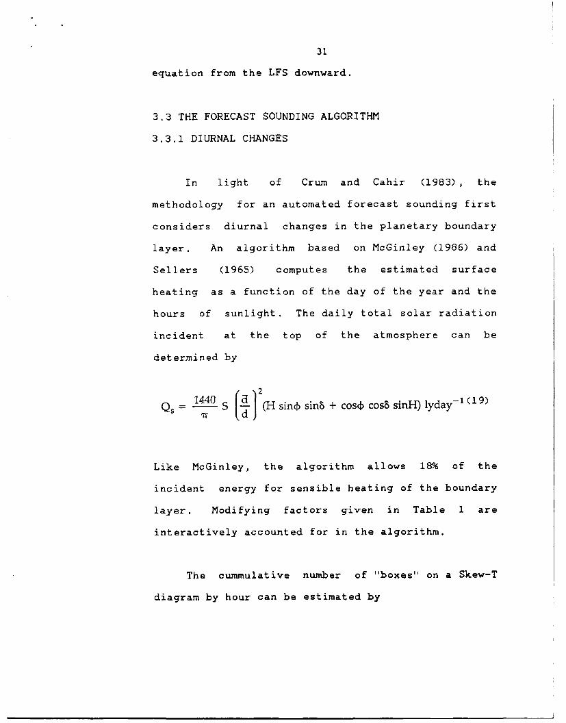
hours of sunlight. The daily total solar radiation

incident at the top of the atmosphere can be

determined by

Qs - 1440 S (H sind sinb + coscf cosS sinH) lyday - (19)

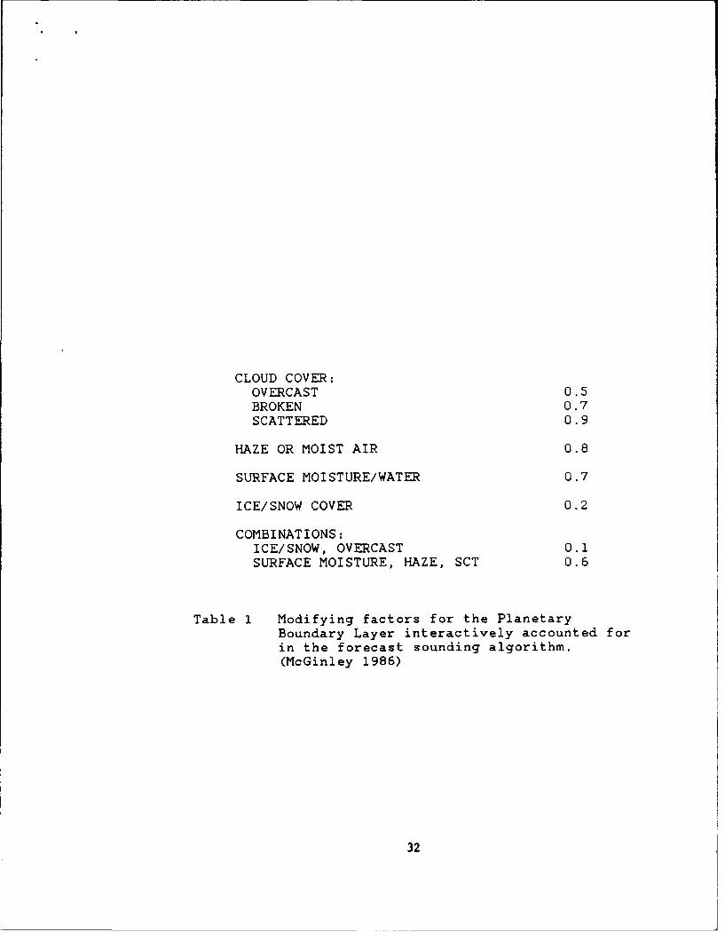
Like McGinley, the algorithm allows 18% of the

incident energy for sensible heating of the boundary

layer. Modifying factors given in Table 1 are

interactively accounted for in the algorithm.

The cummulative number of "boxes" on a Skew-T

diagram by hour can be estimated by

CLOUD COVER:OVERCAST 0.5BROKEN 0.7SCATTERED 0.9

HAZE OR MOIST AIR 0.8

SURFACE MOISTURE/WATER 0.7

ICE/SNOW COVER 0.2

COMBINATIONS:ICE/SNOW, OVERCAST 0.1SURFACE MOISTURE, HAZE, SCT 0.6

Table 1 Modifying factors for the PlanetaryBoundary Layer interactively accounted forin the forecast sounding algorithm.(McGinley 1986)

32

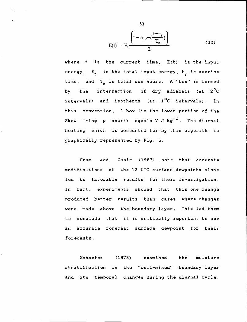
33CO'r t t220E(t) =E t 2 S(0

where t is the current time, E(t) is the input

energy, Et is the total input energy, tr is sunrise

time, and T is total sun hours. A "box" is formed

by the intersection of dry adiabats (at 2°C

intervals) and isotherms (at 1 0C intervals). In

this convention, 1 box (in the lower portion of the-i

Skew T-log p chart) equals 7 J kg . The diurnal

heating which is accounted for by this algorithm is

graphically represented by Fig. 6.

Crum and Cahir (1983) note that accurate

modifications of the 12 UTC surface dewpoints alone

led to favorable results for their investigation.

In fact, experiments showed that this one change

produced better results than cases where changes

were made above the boundary layer. This led them

to conclude that it is critically important to use

an accurate forecast surface dewpoint for their

forecasts.

Schaefer (1975) examined the moisture

stratification in the "well-mixed" boundary layer

and its temporal changes during the diurnal cycle.

, 8c

i

|I

o

8 I

-I

I

Fig. 6 Idealized energy input by surface heating(shaded area is one energy box). Totlheat realized is 50 boxes ( 350 J kg )At is time from sunrise. E is energyrealized for a given At (in boxes).(McGinley 1985)

34

35

The quotient of the mean mixing ratio in the lowest

100 mb to the surface mixing ratio, R, was computed

for 251 samples composed of tower and National

Weather Service (NWS) soundings. Schaefer found

that the mean difference of the quotient between

sounding times ( 6 and 12 local) decreased by an

average of 10%. In the afternoon it is sensibly

constant. From his conclusion, a forecast mean

mixing ratio for the mixed layer can be determined

knowing the forecast surface dewpoint. The 12 UTC

boundary layer dewpoints are then adjsted to the

computed afternoon mean mixing ratio.

3.3.2 MIDDLE AND UPPER LEVEL CHANGES

Changes to the middle and upper levels can be

estimated by first determining the mean geostrophic

advection of temperature for a layer from the 12 UTC

sounding using the relationship

T2fA (21)= R In p,/p.

given the geostrophic wind direction and speed at

the top and bottom of the layer, Vlower and Vlower upper

This method assumes that the winds at and above 700

mb are geostrophic. The area, A, is determined from

36

the triangle formed by these two wind vectors and

the thermal wind vector derived in the same layer.

The Coriolis force, f, dry air gas constant, R, and

the pressure values, pupper and Plower' for the

respective wind levels are the other variables.

The forecast temperature value is simply

calculated by adding some fraction (15%) of the mean

geostrophic temperature advection over a certain

number of hours to the original mean temperature

from the 12 UTC layer. After the forecast sounding

is created it is checked for superadibatic lapse

rates. If any are found, the layers are adjusted

according to a scheme by Haltiner and Williams

(1980) which conserves the total energy.

3.4 VALIDATION TECHNIQUES

For the purposes of this investigation, it is

necessary to apply representative atmospheric

profiles to the events which will be used to

validate the methodologies. For a hail or wind

event to be considered in this investigation, the

event must have occured within 3 hours of sounding

time and within 100 km of the rawinsonde launch

site. This proximity criteria is similar to that

37

used to select proximity soundings described by

Maddox (1973) and Leftwich (1984). The largest

hailstones and strongest gusts recorded in the Storm

Data records for a given event were assumed to be

representative of the maximum potential severity for

that particular storm. This one assumption possibly

contributes the largest source of error in this

study since both the largest hailstone or strongest

gust for a particular storm may not have been

observed. In fact, many wind gust entries in the

Storm Data records were estimates. Despite possible

errors, this investigation assumed the extreme

values to be reasonable estimates of ground

"truth". Table 2 was used to convert many of the

descriptive hail sizes to specific diameters.

The primary field experiment data considered

are;

1. PRE-STORM, conducted in the Kansas-

Oklahoma area from 1 May 1985 to 27

June 1985.

2. AVE-SESAME I, conducted in the Texas-

Oklahoma area 10-11 April 1979.

3. AVE-SESAME II, conducted in the Texas-

Oklahoma area 19-20 April 1979.

Penny - 3/4" diameterDime - 3/4" diameterNickel - 1" diameterQuarter - 1" diameterAnthony dollar - 1 1/4" diameterHalf dollar - 1 1/4" diameterWalnut - 1 1/2" diameterGolfball - 1 3/4" diameterHen egg - 2" diameterTennis ball - 2 1/2" diameterBaseball - 2 3/4" diameterTea cup - 3" diameterGrapefruit - 4" diameterSoftball - 4 1/2" diameter

Table 2 Conversion table of descriptive hailsizes to actual measured diameters.(Doswell 1985)

38

39

Since the majority of the soundings used during

Fawbush and Millers' investigation were from the

Midwest, soundings from other sections of the

country such as the Northeast, Southeast, etc. were

included in the study. Storm Data records were

used to identify possible hail and wind events.

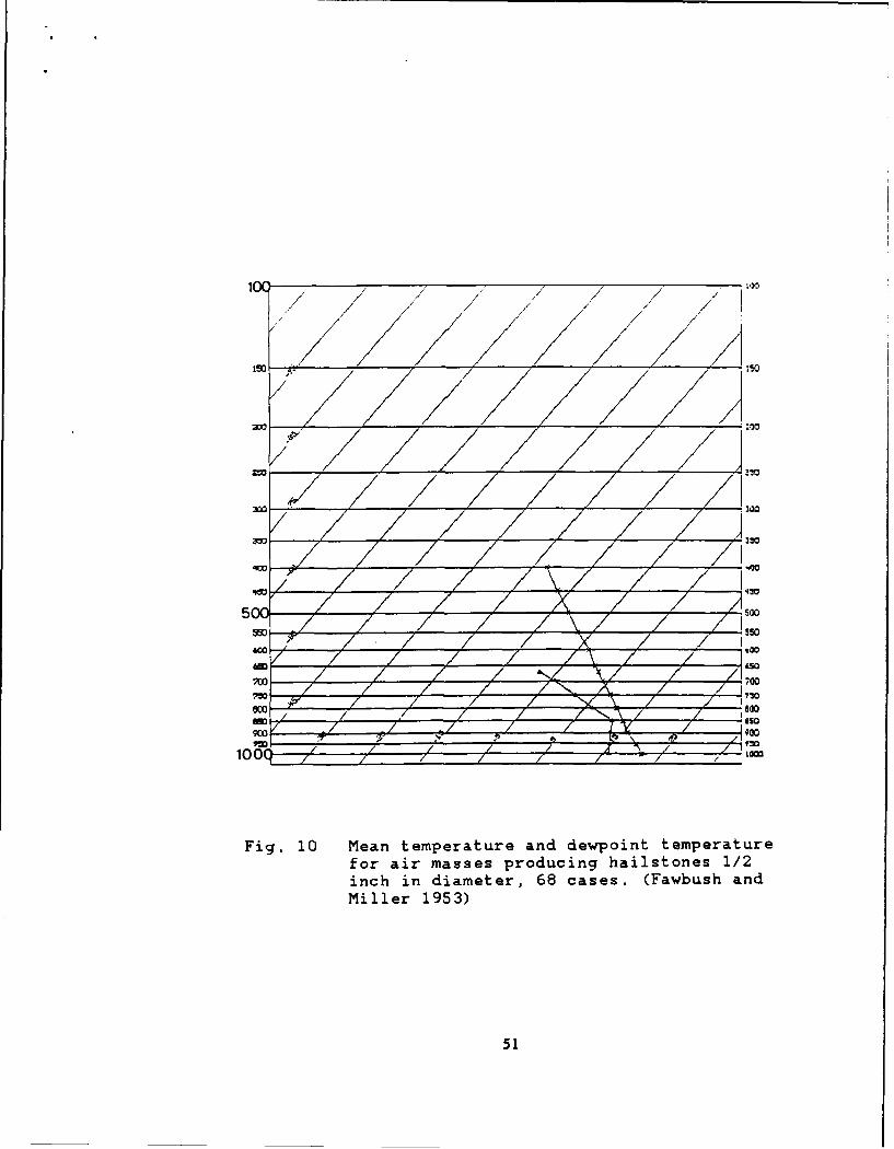
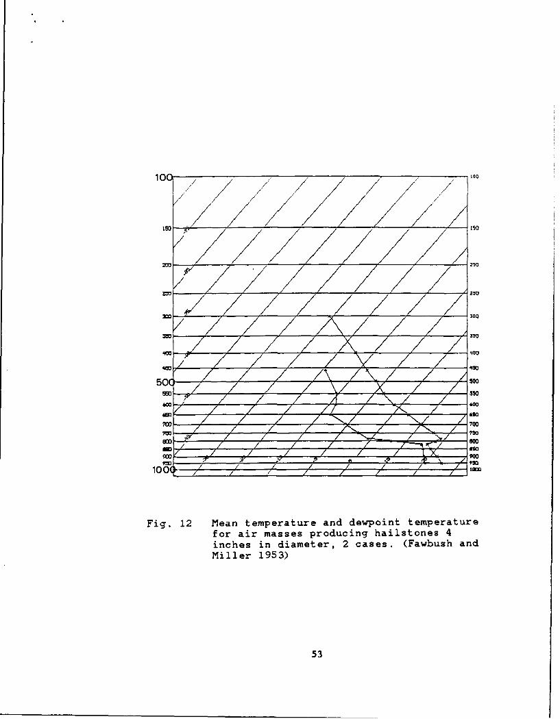
The final validation procedure for the hail

algorithm examines composite hailstorm soundings

calculated by Fawbush and Miller (1953). Fawbush and

Miller examined composite soundings for air masses

which produced one-half, one, and four inch hail.

For each composite sounding, the data will be used

to verify the proposed hail methodology in two

respects: the composite soundings will be applied to

the algorithms for (1) verification purposes, and

(2) to perform a sensitivity check on the variables

used in computing hail size such as the drag

coefficient, density of hail, and level of hail

formation.

Validation of the forecast sounding required

applying the algorithm to a 12 UTC sounding which

precedes a hail/wind event and satisfies the

hail/wind proximity sounding requirements.

Estimates of hail and wind from the forecast

.40

sounding were compared with estimates obtained from

the proximity soundings.

3.5 THE SOUNDING ANALYSIS PACKAGE

Accurate prediction of hail size and

thunderstorm surface wind gusts require a

forecaster's ability to first determine the

likelihood of convection. Understanding the

character-istics of the atmosphere, such as the

stability, positive energy, presence of a lid, and

equilibrium level, etc., for both the 12 UTC profile

as well as the forecast sounding will aid the

forecaster in this determination. In addition to

estimated potential hail size and thunderstorm

surface wind gust velocities, various stability

parameters are routinely available as part of the

sounding analysis algorithm to assess the probabilty

of convection as well as to prognose the degree of

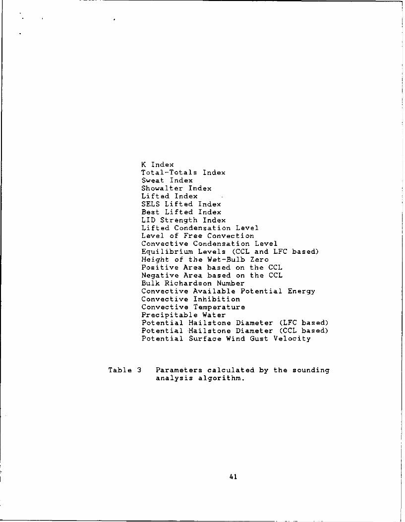
severity (Table 3). These additional thermodynamic

variables were used in this study to help understand

the structure of the sounding as well as to

determine the significance and utility of the

forecast sounding. .ppendix A describes how each of

the parameters in Table 3 are computed.

K IndexTotal-Totals IndexSweat IndexShowalter IndexLifted IndexSELS Lifted IndexBest Lifted IndexLID Strength IndexLifted Condensation LevelLevel of Free ConvectionConvective Condensation LevelEquilibrium Levels (CCL and LFC based)Height of the Wet-Bulb ZeroPositive Area based on the CCLNegative Area based on the CCLBulk Richardson NumberConvective Available Potential EnergyConvective InhibitionConvective TemperaturePrecipitable WaterPotential Hailstone Diameter (LFC based)Potential Hailstone Diameter (CCL based)Potential Surface Wind Gust Velocity

Table 3 Parameters calculated by the soundinganalysis algorithm.

41

4. RESULTS AND DISCUSSION

A sounding analysis was completed for each

proximity sounding in this study, an example of

which is shown in Table 4. Each analysis includes

hail estimates computed by the updated Fawbush-

Miller hail technique (AWS TR-200) and the Pino-

Moore hail algorithms (CCL and LFC) along with

computed wind gusts based on Fawbush-Miller (AWS TR-

200), Foster (1958), and Anthes (1977) . In addition

to these estimates, various stability parameters and

thermodynamic energy values relative to each

atmospheric profile are included. Appendix A

briefly describes the method for computing each

parameter.

For each sounding analysis, two hail size

estimates are calculated from the Pino-Moore

algorithms, based on the positive areas above the

LFC and the CCL. If the surface temperature for

each proximity sounding was within 2 F of the

convective temperature or greater and the lid

strength term was less than or equal to 2 0 C, the

hail stone size estimate calculated from the CCL was

used. Graziano and Carlson (1988) found a practical

threshold for convective penetration of the lid

42

SI - -5.0 SWEAT INDEX = 325.6KI - 37.5 TTI - 53.7LI - -4.9 LID STRENGTH - 1.01BEST LIFTED INDEX - -4.5SELS LI - -999.0MAX TEMP BASED ON SELS LI - -999.0 deg F

THE CONVECTIVE TEMP BASED ON THE CCL - 76.0 deg FThe CCL Is at 850.0 mbThe EL (CCL based) Is at 202.4mb -54.2 deg CThe LCL(BL) Is at 833.3 mbThe LFC Is at 819.0 mb 13.4 deg CThe EL (LFC based) Is at 213.0 mb -54.3 deg CCONVECTIVE AVAILABLE POTENTIAL ENERGY - 1680.5 J/kgCONVECTIVE INHIBITION m 12.5 J/kgVERTICAL WIND SHEAR (6000 M - 500 M) - 3.7X e-03 s-1BULK RICHARDSON NUMBER - 8.3POSITIVE AREA (CCL BASED) - 2622.4 J/kgNEGATIVE AREA (CCL BASED) - 3.0 J/kg

PRECIPITABLE WATER - 1.13 InHEIGHT WET BULB ZERO (AGL) - 9534.9 ftW MAX BASED ON LFC - 24.18 m/sDIAM OF HAIL FROM LFC - 5.09 cm C 5.23 cm)W MAX BASED ON CCL - 31.03 m/sDIAM OF HAIL FROM CCL - 8.35 cm C 8.44 cm)DIAM OF HAIL (TR-200) - 4.23 cm C 4.23 cm)SFC WIND GUST BASED ON F-M - 74.9 ktsSFC WIND GUST BASED ON FOSTER - 72.4 ktsSFC WIND GUST BASED ON ANTHES - 40.2 kts

Table 4 Example of the Pino-Moore soundinganalysis. Note: for hail sizes, estimatesin parentheses are values prior tomelting.

43

44

occurs at a lid strength of 2.00C. If these

criteria were not met, the LFC estimate was used.

4.1 HAIL SIZE FORECAST VALIDATION

4.1.1 COMBINED CASES

Fifty-eight cases selected from PRE-STORM, AVE-

SESAME I, AVE-SESAME II and events from July and

August 1986 were used in validating the hail

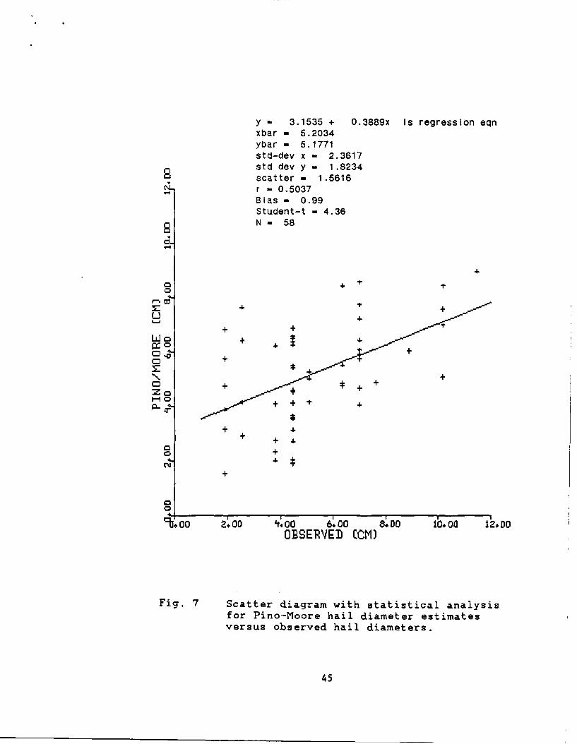
algorithms. Figures 7 and 8 contain the results of

the computed hailstone diameters according to the

Pino-Moore and Fawbush-Miller methods compared with

the observed hailstones. Also shown with each

scatter diagram are statistical analyses which

include the linear regression equation, the means of

the observed and estimated values (xbar and ybar),

the standard deviations (std-dev x and std-dev y),

the scatter, the correlation coefficient (r), the

bias, and the Student-t statistic value for both

sets of data.

Comparing Figure 7 and 8, the Pino-Moore

algorithm proved to be much more successful in

estimating the actual size of the hail events. The

set of data represented in Fig. 7 resulted in a

Student-t statistic significant at the 0.5% level

y 3.1535 + 0.3889x Is regression eqnxbar - 5.2034ybar - 5.1771std-dev x - 2.3617std dev y - 1.8234

8scatter - 1.5616r - 0.5037Bias - 0.99Student-t - 4.36

8~ N- 58

'-44

46..

+

:z ++ + 4 +

~+ + 4-

+ 4.

o +4*

9J.00 L:.0 OD 00 6. 00 8.D0 10#0a 12.D0OBSERVED (CM)

Fig. 7 Scatter diagram with statistical analysisfor Pino-Moore hail diameter estimatesversus observed hail diameters.

45

y 1.6357 + 0.1254x Is regression eqnxbar - 5.2034ybar - 2.2879std-dev x - 2.3617std dev y - 1.5620

*scatter - 1.5204r - 0.1895Bias - 0.44Student-t - 1.44

SN- 58

PC

+. +

+ 4-

.4 ......I

9'0 #1 t, 00 6. 00 8. DO b a 1'2. DO

OBSERVEDl CCM)

Fig. 8 Scatter diagram with statistical analysisfor Fawbush-Miller hail diameter estimatesversus observed hail diameters.

46

47

whereas the data represented by Fig. 8 resulted in a

Student-t statistic significant at the 10% level.

Additionally, the Fawbush-Miller method did not

indicate severe storm potential (greater than 1.91

cm) for 24 of the 58 cases studied while the Pino-

Moore algorithm missed only one of the 58 cases.

These results raise doubt as to the validity of

Fawbush and Miller's (1953) statement that

"hailstones maintain their size for at least 9000

feet of freefall, after which rapid melting and

disintergration take place". Some of the error in

determining hailstone size with the Fawbush-Miller

technique can be attributed to the way the positive

area is calculated (Fig. 1) . Their triangle method

only approximates the actual positive area.

However, the results obtained in this study suggest

that their premise concerning rapid melting and

disintegration may not be as significant or dramatic

as they state.

Melting rates obtained from the Pino-Moore

method varied from approximately 5% for the largest

stones to as much as 100% for stones less than 1 cm

in diameter. These results are in agreement with

those reported by Mason (1956), Macklin (1963), and

48

Auer and Marwitz (1972). While Fawbush and Miller

suggest dramatic melting for large hailtones with a

corresponding WBZ height greater than 10,500 feet,

our algorithm indicates that these larger stones

undergo the least amount of melting of any of the

hailstones. As the size of the stone decreases,

melting rates increase. Hailstones initially having

diameters less than 1 cm at the level of hail

formation very seldom reach the surface even though

these stones fall within the storm's protective

downdraft.

The results of the Fawbush-Miller method was

statistically analyzed disregarding their correction

due to melting (Fig. 9). The linear regression

equation, correlation coefficient (.22 vs. .19),

bias (.76 vs. .44), and the t-statistic (sigiiificant

at the 5% level) all indicate that the Fawbush-

Miller technique produced better estimates for the

58 cases in this study when melting was neglected.

In addition, the Fawbush-Miller method indicated

severe potential for 49 of the 58 cases missing only

9 severe situations.

y - 3.0679 + 0.1697x Is regression eqnxbar - 5.2034ybar - 3.9507std-dev x - 2.3617std dev y - 1.8221scatter - 1 .7621

_ r - 0.2199Bias - 0.76Student-t - 1.69

8 N -58

I4

.-

4 .

++

4-4

-4J+-4

-4o

4- +

C0 +

9.'00 2-.00 't'.00 6' .00 ;5'. D ib. oa 12.D0OBSERVEDl CCM)

Fig. 9 Scatter diagram with statistical analysisfor Fawbush-Miller hail diameter estimateswithout melting.

49

50

4.1.2 COMPOSITE SOUNDINGS

Fawbush and Miller's (1953) hail study produced

composite soundings for one-half inch, one inch, and

four inch hail (Fig. 10, 11, 12). The dewpoint

profile for each of these composite soundings had to

be calculated since the soundings contained in their

original paper included only the mean temperature

and wet-bulb curves. Heights were hydrostatically

computed. Table 5 shows the results of the

calculated hailstone sizes for each of the

soundings. Since no other synoptic data was

included with these composite soundings and since

the convective temperatures for each of the

soundings were fairly high, much higher than the

surface temperatures of the soundings, the hailstone

sizes computed by the LFC-based CAPE were taken as

being representative of the storms which developed

under these thermodynamic conditions.

As indicated in Table 5, values computed by the

Pino-Moore algorithm for the four inch and one inch

composite soundings were closer to the observed

hailstone values than those estimated by Fawbush-

Miller. Both methods did poorly in the estimates

for the half-inch composite sounding. One reason

/5 IS

500 Soo

.00

Aso

100 / 00

Fig. 10 Mean temperature and dewpoint temperaturefor air masses producing hailstones 1/2inch in diameter, 68 cases. (Fawbush andMiller 1953)

51

10 too0

330

9w q30

50C Soo

59/ 550

6~C 600

6M5

7W 70

k 16000

100

Fig. 11 Mean temperature and dewpoint temperaturefor air masses producing hailstones 1 inchin diameter, 25 cases. (Fawbush and Miller1953)

52

10 //

///

= / -/ -A3

500 -Soo

001 70

sio

Fig. 12 Mean temperature and dewpoint temperaturefor air masses producing hailstones 4inches in diameter, 2 cases. (Fawbush andMiller 1953)

53

FAWBUSH-MILLER PINO-MOORE

DIAMETER/ERROR DIAMETER/ERROR

HALF-INCH COMPOSITE (1.27 cm) 2.45 (+1.18) 0.17 (-1.10)

ONE-INCH COMPOSITE (2.54 cm) 3.24 (+0.70) 3.13 (+0.59)

FOUR-INCH COMPOSITE (10.16 cm) 3.11 (-7.01) 12.27 (+2.11)

Table 5 Results of the composite sounding hailsize estimates as computed by Pino-Mooreand Fawbush-Miller techniques.

54

55

why the Pino-Moore method underestimated the half-

inch composite sounding could be attributed to our

assumption of the drag coefficient being 0.6. As

Matson and Huggins (1980) found in their study,

small hailstones in this range may exhibit larger

drag coefficients because of the increase in the

irregularity of the hailstone shapes. The sounding

analysis was recomputed with a drag coefficient of

0.87 and the Pino-Moore method resulted in a

hailstone diamater of 0.68 cm after the effects of

melting.

In light of these results, the Pino-Moore

method should be tested for hail events less than

1.91 cm. It was not tested in this study since the

hail events were all greater than 3/4 of an inch in

diameter. A future test should determine which drag

coefficient, 0.60 or 0.87, results in the best

estimates. If the test shows in favor of a drag

coefficient of 0.87 for observed hailstones less

than 1.91, the algorithm could easily be modified to

allow a value of 0.87 for small hailstones and 0.60

for hailstones greater than 1.91 cm.

56

4.2 CONVECTIVE WIND GUST VALIDATION

Similar to the hail size validation, three

techniques for estimating convective wind gusts were

tested for 47 cases (Fig. 13, 14, 15). The

observed wind gusts were identified from the Storm

Data records. For a significant number of cases,

the wind gusts were reported as estimates. Although

a statistical analysis was completed for each set of

data, the results of these analyses were

questionable due to; (1) the small range of observed

values, (2) the uncertainty of the

representativeness of the observed gusts to the

actual severity of the storms which produced them,

and (3) the fact that some of the validating gust

speeds were estimates.

Statistical analyses aside, one striking

feature evident in the Fawbush-Miller and Foster

scatter diagrams is the amount of vertical

scattering. This raises some doubt as to the

operational utility of these methods. While results

of the Anthes' method spm to underforecast

convective gust events slil- ly (bias = 0.96)

compared to the significant overforecasting of the

other techniques (bias = 1.29, 1.23), the Anthes'

y - 63.3675 + 0-2103x Is regression eqnxbar - 58.8936ybar - 75.7532std-dev x - 8.3203

_ std dev y - 26.6318_ scatter - 26.2899-4 r - 0.0657

Bias - 1.29Student-t - 0.44

+ N- 47-4 +

U

IA

++

4. +

E3

IL +4 ++

+0S

0

F-. DO6U0%0.0 8,0 ~ 0 a 10C-ER EI CI' T)4

Fig. 13Satrdarmwthsaitclaayifo wns simtd y ote etovessosretidgss

LLI +57

y - 56.0462 + 0.2817x Is regression eqnxbar - 58.8936ybar - 72.6383

std-dev x - 8.3203

3 std dev y - 20.4660_ scatter - 20.11394r - 0.1145

Bias - 1.23Student-t = 0.77

EN - 47

L6--

.4.

U A 4.

CV +

N0O- o 5b00 6b.O .0 70# 800 M O0 ?o0. O0 00 OBSERVED CKT)

Fig. 14 Scatter diagram with statistical analysis

for winds estimated by Fawbush-Miller

method versus observed wind gusts.

58

y - 53.4361 + 0.0506x Is regression eqn

xbar - 58.8936

ybar - 56.4170std-dev x - 8.3203std dev y - 9.8820scatter - 9.7674r - 0.0426Bias - 0.96Student-t - 0.29N - 47

C5CL

LL)

W + +

0 4+ +7 + + t

. -. + *Lr + $ +

T4. 4

0+

z O 4. +

050,0 DO 60.00 70o 0 80, 0 0-0 00,0

OBSERVED CKT)

Fig. 15 Scatter diagram with statistical analysis

for winds estimated by Anthes method

versus observed wind gusts.

59

60

technique displays considerably less scatter. Based

on scattering alone, the Anthes method seems to

offer more reliability in an operational setting.

A possible reason for the Anthes' method

underestimation of the winds lies in the algorithm's

neglect of the water-loading term above the LFS.

The integration of all three terms in Anthes'

vertical velocity equation assumes no contribution

of any of the terms above the LFS. Precipitation

fallout from above the LFS into the forming

downdraft would result in strengthening the

downdraft.

4.3 SENSITIVITY STUDY OF KEY VARIABLES

The values of the hailstone drag coefficient,

density, and the level of hail formation used in the

Pino-Moore method were taken from a wide range for

values offered by the various literature reviewed.

While the results of this study appear to be well

supportive of our values of these variables, the

author wanted to show the importance of these

variables to the resultant hail estimates. Table 6

shows the wide range of hail estimates obtained by

varying the hailstone drag coefficient, density, and

DRAG COEFFICIENT(density of ice = 0.90)(level of hail formation Tp = -10 C)

0.45, (smooth sphere) 5.74 cm0.60 (rough sphere) 7.74 cm0.70 9.05 cm0.87 (Matson and Huggins) 11.29 cm

DENSITY OF HAILSTONE(drag coefficient = 0.60)(level of hail formation Tp = -10 C)

-30.70 g cm_3 (Foster and Bates) 9.99 cm0.89 g cm_ 3 (Matson and Huggins) 7.82 cm0.90 g cm_3 7.74 cm0.92 g cm 7.56 cm

LEVEL OF HAIL FORMATION(drag coefficient = 0.60)(density of ice = 0.90 g cm - )

Tp = -5.00Co 6.68 cmTp = -10. 0 C 7.74 cmTp = -15.00C 8.63 cm

= Values used by Pino-Moore

Table 6 Hailstone diameters computed by varyingdrag coefficient, hailstone density, andlevel of hail formation.

61

62

level of hail formation. This sensitivity study was

thapplied to the 0000 UTC May 27 , 1986 Enid,

Oklahoma sounding obtained during PRE-STORM. The

verifying hailstone size for this particular

sounding was 6.99 cm.

As indicated by Table 6, increasing the drag

coefficient from 0.60 to 0.87 (a 45% increase)

results in about a 46% increase in hail diameter.

This one variable alone demonstrates the. high

sensitivity inherent with the Pino-Moore algorithm.

Increasing the density of the hailstone from .70 g-3 -3

cm to 0.92 g cm (31%) decreases the diameter

24%. A diameter increase of 29% results from

raising the level of hail formation from -5.0 C to -

15.0 0 C.

4.4 FORECAST SOUNDING UTILITY

Fifteen 1200 UTC soundings were identified

during the validation of the hail methodologies as

possible test cases for the forecast sounding

validation. These soundings preceded an

afternoon/early evening hail event for which a

proximity sounding was available. Sounding analyses

were performed on: (1) the unadjusted 1200 UTC

63

sounding, (2) an adjusted 1200 UTC sounding

considering diurnal changes in the mixed layer, and

(3) a forecast sounding adjusting both the mixed

layer as well as the middle and upper layers.

In adjusting the diurnal changes in the mixed

layer, the algorithm requires the operator's input

of several parameters. The algorithm asks the

operator for:

(1) the current date,

(2) the modification factor (Table 1),

(3) the station's latitude and longitude,

(4) the number of hours past sunrise convection

is expected.

Based on this input, the algorithm computes the

forecast surface temperature for the time of

convection. The program then indicates this

temperature. If the operator does not agree with

this estimate, the operator may input his/her own

temperature. Based on the temperature input into

the program, the lowest part of the sounding is

adjusted to account for this energy as shown earlier

in Fig. 6. The algorithm then asks for the expected

surface dewpoint at time of convection. This

dewpoint is used in adjusting the moisture profile

in the mixed layer. If an inversion is present just

64

above the mixed layer, the surface dewpoint is

adjusted and moisture lapse rate in the mixed layer

is not adjusted. This condition is addressed in

section 4.4.1. The top of the mixed layer is

determined during the thermal adjustment portion of

the algorithm. In validating the adjusted

soundings, the surface temperature and dewpoint

temperature of the corresponding proximity sounding

was used.

Table 7 contains the results of the hailstone

diameter estimates based on the various adjusted and

unadjusted soundings. A surprising result indicated

by the mean errors is that while the proximity

sounding underestimated the diameters by 1.18 cm,

both adjusted soundings produced better mean errors

than the proximity soundings as well as the 1200 UTC

soundings. An example of the decision making

process associated with using the forecast sounding

algorithm is given in section 4.4.

Of the fifteen soundings analyzed in this

section, two were associated with strong convective

gust events. Both 1200 UTC sounding analyses did

not indicate potential for convectively-driven

downdraft gusts for all three techniques. For the

FCSTRAOB FCSTRA013

OBSERVED 1200UTC BDY ONLY BDY +, GEO PROXIMITY

3.81 0.00C-3.81) 4.11C+0.30) 5.60(+1.79) 2.75(-1.06)

6.35 1.71(-4.64) 3.58(-2.77) 4.16(-2.19) 8.43(-2.08)

4.45 8.04(+3-59) 7.12(+2.67) 7.70(+3.25) 6.48(-2.03)

10.16 2.62(-7.54) 4.94(-5.22) 6.74(-3.42) 5.08(-5.08)

4.45 4.61C+0.16) 4.82C+0-37) 5.20C-0.75) 3.60(-0.85)

8.89 4.39(-4.50) 5.40(-3.49) N/A 6.04(-2.85)

6.35 2.36(-3.99) 5.35C-1.00) 6.36(+0.01) 4.83(-1.62)

6.99 2.94(-4.05) 5.55(-1.44) 6.63C-0.36) 5.92(-1.07)

3.81 3.67C-0.14) 3-86C+0.05) 4.46C-0.65) 4.08(+0.27)

4.45 1.98(-2.47) 5.14C+0.69) 4.77(+0.32) 6.38(+1.93)

3.81 1.98C-1.83) 6.58(-2.77) 6.30(+2.49) 2.33(-1.48)

4.45 0.00C-4.45) 2.38(-2.07) 2.46(-1.99) 3.56(-0.89)

3.81 0.14(-3.67) 0.76(-3.05) 3.89C+0.08) 2.02(-1.79)

6.35 6.85C+0.50) 6.09(-0.26) 4.60C-1.75) 4.75(-1.60)

4.45 8.86(+4.41) 7.79(+3.34) 8.10C+3.65) 6.87(+2.42)

TOTAL ERROR (-32.43) (-14.65) C+0.48)* (-17.68)

MEAN ERROR (-2.16) (-0.98) C+0.03)* (-1.18)

*Total and mean error for 14 cases only.

Table 7 Validation results for the forecastsounding algorithm. Numbers inparentheses indicate error.

65

66

forecast soundings which included geostrophic

thermal advection, severe wind gust potential was

indicated by the Fawbush-Miller and the Foster

techniques while the Anthes technique favored severe

potential for one of the cases with near severe

threshold for the second case. The proximity

soundings indicated severe potential for all three

techniques.

4.4.1 LIMITATIONS AND WEAKNESSES

While the forecast sounding proved its utility

for severe events where dynamics played an

overwhelming role in the development of the severe

convection, interrogation of the resultant forecast

soundings as compared to the corresponding proximity

sounding revealed several weaknesses with the

forecast sounding algorithm. In situations where

very little heating took place, the adjusted

sounding resulted in a very shallow mixed layer.

This in turn allowed for geostrophic thermal

advection to occur at low levels which was usually

too strong. In similar situations where an

inversion was present just above the adjusted mixed

layer, the adjusted moisture structure of the mixed

layer as computed by Schaefer (1975) resulted in

67

too dry a layer. To correct for this, the algorithm

was modified to "look" for the presence of an

inversion (an increase in temperature of at least

1°C) in the three levels above the mixed layer. If

an inversion exists, the algorithm does allow for a

change in the surface dewpoint but does not adjust

the moisture lapse rate in the mixed layer.

The diurnal heating algorithm is best suited

for quiescent surface conditions in which there is

weak or little low level thermal advection. In some

of the cases, especially during the early spring

months, low level cold air advection inhibited the

solar diurnal heating. The predicted maximum

surface temperature was approximately 5 C too warm.

Although low level cold air advection can lead to

overestimation of the effects of diurnal heating,

low level warm air advection does not seem to affect

the solar heating significantly.

During the summer months, the role of the

geostrophic thermal advection in the modification of

the upper air thermal structure may not be as

prominant as during the spring months. The final

version of the algorithm accounts for these

situations and allows the operator to neglect this

68

advection.

Applying 12 hour forecast changes to the middle

and upper levels using the geostrophic thermal

advection assumes the wind profile over these levels

does not change very much. In reality, however, the

wind profile, especially during the spring months,

may undergo considerable changes. As a result,

estimates of the geostrophic thermal advectivion may

be best applicable when forecasting changes for a

only few hours, say 4-6 hours.

4.5 CASE STUDY

On 20 February 1989, severe thunderstorms

battered eastern Louisiana and western Mississippi

during the late afternoon and early evening hours.

In addition to spawning tornados and producing

damaging downdraft winds, large hail accompanied

these storms. Hail estimated at 2 inches (5.08 cm)

fell at Vicksburg, Mississippi. To further

illustrate the operational utility of the Pino-Moore

sounding analysis and the forecast sounding

algorithm, a case study of the hail event at

Vicksburg was completed after-the-fact.

69

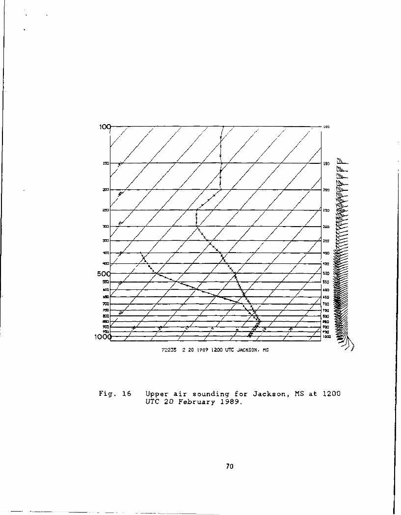
An analysis was performed for the 1200 UTC 20

February sounding (Fig. 16) for Jackson,

Mississippi. This sounding meets the proximity

sounding requirements for this hail event. The 983

mb level data was deleted as it appeared

inconsistent. Table 8 is the sounding analysis of

Fig 16. The morning Lifted Index was fairly high

not indicative of deep convection. The Pino-Moore

hail algorithm estimated possible hail of nearly 3/4

inch diameter, assuming a convective temperature of

770F was reached. The Fawbush-Miller technique

estimated hail at less than 1/2 inch. Note also

that the wind gust estimates for all three

techniques did not favor downdraft conditions.

The forecast sounding was run twice, one

allowing diurnal changes as well as geostrophic

thermal advection while the second run allowed

diurnal changes only (Fig. 17 and 18,

respectively). To produce the forecast soundings,

the following information was interactively input

into the algorithm.

1. The date.

2. A modification factor of 0.5 (overcast

conditions) since a stratus deck covered

2m~

21o0

50 300

3:0

9/ 7Z-7-100

09~

600 10fisa

00 / / / /'i0

72235 2 20 1989 1200 UTC JACKSON, MS 2

Fig. 16 Upper air sounding for Jackson, MS at 1200UTC 20 February 2989.

70

SI - -1.4 SWEAT INDEX - 301.9

KI = 32.6 TTI - 51.5

LI - 5.2 LID STRENGTH - 3.24

BEST LIFTED INDEX - 3.7

SELS LI - -939.0

MAX TEMP BASED ON SELS LI - -999.0 deg F

THE CONVECTIVE TEMP BASED ON THE CCL - 77.0 deg F

The CCL Is at 824.2 mb

The EL (CCL based) Is at 279.8mb -48.0 deg C

The LCL(BL) Is at 946.6 mbThe LFC Is at -999.0 mb -999.0 deg C

The EL (LFC based) Is at -999.0 mb -999.0 deg C

CONVECTIVE AVAILABLE POTENTIAL ENERGY - -999.0 J/kg

CONVECTIVE INHIBITION - -999.0 J/kgVERTICAL WIND SHEAR (6000 M - 500 M) - 4.7X e-03 s-1

BULK RICHARDSON NUMBER - -99.9POSITIVE AREA (CCL BASED) - 882.3 J/kg

NEGATIVE AREA (CCL BASED) - 0.2 J/kg

PRECIPITABLE WATER - 1.02 InHEIGHT WET BULB ZERO (AGL) - 9290.6 ft

W MAX BASED ON LFC - 0.00 m/s

DIAM OF HAIL FROM LFC - 0.00 cm ( 0.00 cm)W MAX BASED ON CCL - 15.77 m/s

DIAM OF HAIL FROM CCL - 1.64 cm C 1.83 cm)

DIAM OF HAIL (TR-200) - 0.92 cm C 0.92 cm)SFC WIND GUST BASED ON F-M - 0.0 kts

SFC WIND GUST BASED ON FOSTER - 0.0 ktsSFC WIND GUST BASED ON ANTHES - 0.0 kts

Table 8 Sounding analysis for the 1200 UTC 20

February 1989 Jackson, MS sounding.

71

100 Lao

/ / //

150 ISO

___ 200

;o 9,30

50 7 S00am 40

720NA / 700

722Z5 2 20 1989 2'i O0 U7tC JACKSON, MS '

Fig. 17 Forecast sounding (diurnal changes only)for Jackson, MS at 0000 UTC 21 February1989.

72

1000

9w '00

700 700?W 1 7/

-3' 011~

72235 2 20 1?8? 2400O UTC JACKSON, MS

Fig. 18 Forecast sounding (diurnal changes andgeostrophic thermal advection) forJackson, MS at 0000 UTC 21 February1989.

73

74

the region.

3. The station's latitude and longitude.

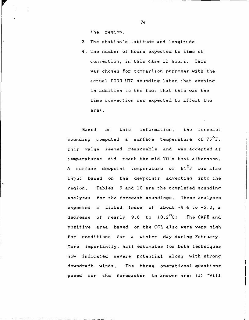
4. The number of hours expected to time of

convection, in this case 12 hours. This

was chosen for comparison purposes with the

actual 0000 UTC sounding later that evening

in addition to the fact that this was the

time convection was expected to affect the

area.

Based on this information, the forecast

sounding computed a surface temperature of 75 F.

This value seemed reasonable and was accepted as

temperatures did reach the mid 70's that afternoon.

A surface dewpoint temperature of 64°F was also

input based on the dewpoints advecting into the

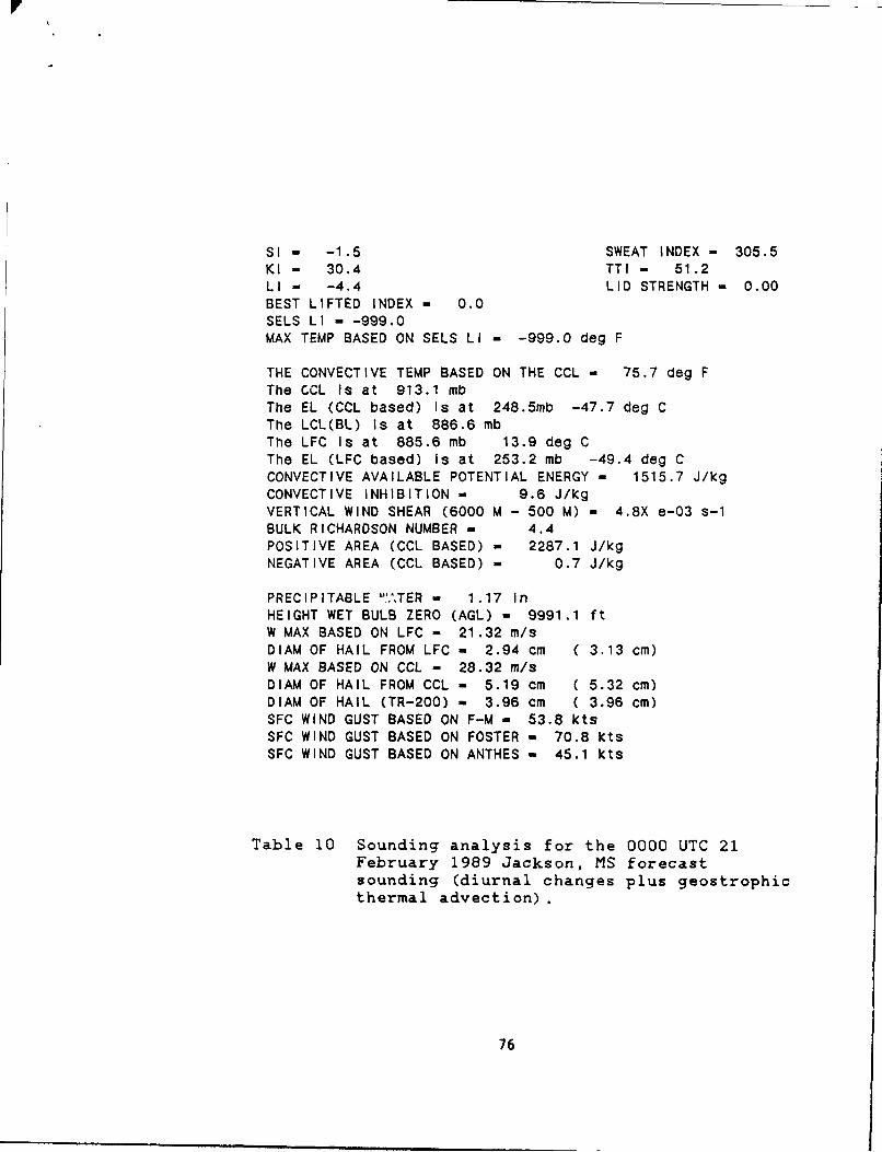
region. Tables 9 and 10 are the completed sounding

analyses for the forecast soundings. These analyses

expected a Lifted Index of about -4.4 to -5.0, a

decrease of nearly 9.6 to 10.2 °C The CAPE and

positive area based on the CCL also were very high

for conditions for a winter day during February.

More importantly, hail estimates for both techniques

now indicated severe potential along with strong

downdraft winds. The three operational questions

posed for the forecaster to answer are: (1) "Will

SI - -2.1 SWEAT INDEX - 329.5

KI - 33.5 TTI - 52.4LI - -5.0 LID STRENGTH - 0.00BEST LIFTED INDEX - 0.0SELS LI - -999.0MAX TEMP BASED ON SELS LI - -999.0 deg F

THE CONVECTIVE TEMP BASED ON THE CCL - 75.7 deg FThe CCL Is at 913.1 mbThe EL (CCL based) Is at 236.7mb -50.6 deg CThe LCL(BL) Is at 886.6 mbThe LFC Is at 885.6 mb 13.9 deg CThe EL (LFC based) Is at 246.2 mb -51.1 deg CCONVECTIVE AVAILABLE POTENTIAL ENERGY - 1794.9 J/kgCONVECTIVE INHIBITION - 0.4 J/kgVERTICAL WIND SHEAR (6000 M - 500 M) - 4.8X e-03 s-1BULK RICHARDSON NUMBER - 5.2POSITIVE AREA (CCL BASED) - 2606.0 J/kgNEGATIVE AREA (CCL BASED) - 0.5 J/kg

PRECIPITABLE WATER - 1.17 inHEIGHT WET BULB ZERO (AGL) - 9357.3 ftW MAX BASED ON LFC - 27.15 m/sDIAM OF HAIL FROM LFC - 4.96 cm C 5.08 cm)W MAX BASED ON CCL - 32.82 m/sDIAM OF HAIL FROM CCL - 7.05 cm C 7.15 cm)DIAM OF HAIL (TR-200) - 4.51 cm ( 4.51 cm)SFC WIND GUST BASED ON F-M - 57.3 ktsSFC WIND GUST BASED ON FOSTER - 53.2 ktsSFC WIND GUST BASED ON ANTHES - 37.1 kts

Table 9 Sounding analysis for the 0000 UTC 21February 1989 Jackson, MS forecastsounding (diurnal changes only).

75

SI - -1.5 SWEAT INDEX - 305.5KI - 30.4 TTI - 51.2LI - -4.4 LID STRENGTH - 0.00BEST LIFTED INDEX - 0.0SELS LI - -999.0MAX TEMP BASED ON SELS LI - -999.0 deg F

THE CONVECTIVE TEMP BASED ON THE CCL - 75.7 deg FThe CCL Is at 913.1 mbThe EL (CCL based) Is at 248.5mb -47.7 deg CThe LCL(BL) Is at 886.6 mbThe LFC Is at 885.6 mb 13.9 deg CThe EL (LFC based) is at 253.2 mb -49.4 deg CCONVECTIVE AVAILABLE POTENTIAL ENERGY - 1515.7 J/kgCONVECTIVE INHIBITION - 9.6 J/kgVERTICAL WIND SHEAR (6000 M - 500 M) - 4.8X e-03 s-1BULK RICHARDSON NUMBER - 4.4POSITIVE AREA (CCL BASED) - 2287.1 J/kgNEGATIVE AREA (CCL BASED) - 0.7 J/kg

PRECIPITABLE "'ATER - 1.17 In

HEIGHT WET BULB ZERO (AGL) - 9991.1 ftW MAX BASED ON LFC - 21.32 m/sDIAM OF HAIL FROM LFC - 2.94 cm ( 3.13 cm)W MAX BASED ON CCL - 28.32 m/sDIAM OF HAIL FROM CCL - 5.19 cm ( 5.32 cm)DIAM OF HAIL (TR-200) - 3.96 cm ( 3.96 cm)SFC WIND GUST BASED ON F-M - 53.8 ktsSFC WIND GUST BASED ON FOSTER - 70.8 ktsSFC WIND GUST BASED ON ANTHES - 45.1 kts

Table 10 Sounding analysis for the 0000 UTC 21February 1989 Jackson, MS forecastsounding (diurnal changes plus geostrophicthermal advection).

76

77

there be thunderstorms later that day?", (2) "Will

they reach severe potential?", and (3) "What hail

and convective gust estimates should be used as

guidance for a hail/wind forecast?". Assuming the

forecaster ran the forecast sounding allowing for

changes due to diurnal heating and geostrophic

thermal advection and performed a sounding analysis

as shown herein, how would he or she answer these

three questions?

The convective temperature indicated by the

sounding analysis indicates 75 F. This was the same

surface temperature computed by the forecast

sounding algorithm. If the forecaster felt a

maximum of 750 was reasonable or if a lifting

mechanism was expected during the afternoon hours,

the answer to the first question would be yes.

Based on the informaton offered by the sounding

analysis, the forecaster could also expect severe

weecher to accompany the thuderstorms. The third

question needs to be answered in order to issue the

severe warning. The results shown in Table 10

should be considered as it was shown in section 4.4

that the hail estimates calculated from forecast

soundings which allowed geostrophic thermal

advection had the lowest mean diameter error. Since

78

the convective temperature could be reasonably

reached, the estimate of 5.19 cm should be used as

guidance for issuing the warning. If this estimate

was used, he or she would have made good decision

since 5.08 cm hail verified. The forecast sounding

also indicated strong convective gusts nearing

severe threshold ( > 55 knots) criteria as estimated

by the Fawbush-Miller and the Anthes methods with

Foster's method indicating severe potential. The

closest convective gust report available at the time

of this investigation was at Alexandria, LA with 52

kts. This wind report, however, does not meet the

proximity criteria and therefore cannot be used as

verification for these estimated wind gusts.

Surface temperatures that afternoon reached

72 F at Jackson with many stations south of

Vicksburg reaching the mid 70's and low 80's just

before convective activity began in the area (Fig.

19). While there is not a reporting station at

Vicksburg, it is likely the temperature in and

around the Vicksburg vicinity reached the mid 70's.

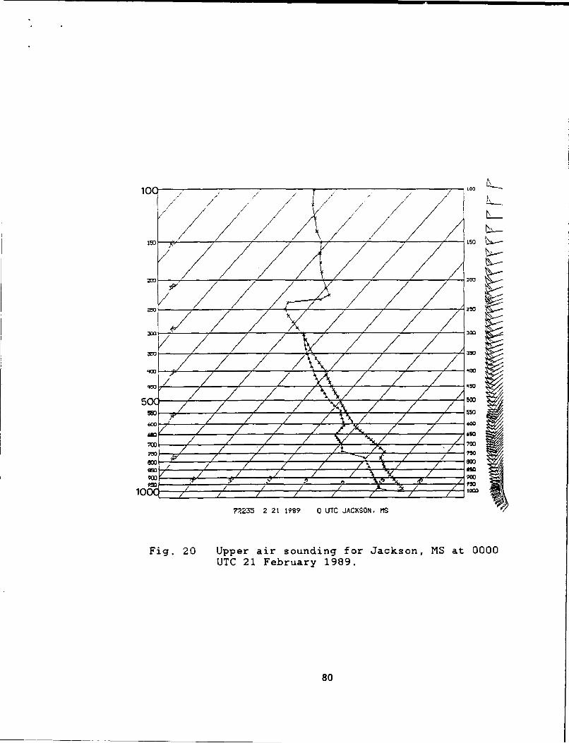
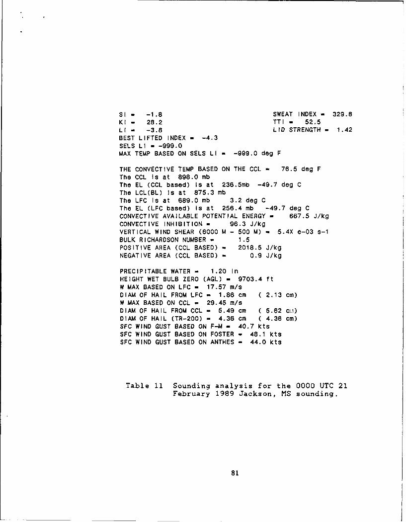
Figure 20 displays the actual 0000 UTC 21 February

sounding from the Jackson launch site. The sounding

analysis, Table 11, is also included. Note the

Lifted Index for the actual evening sounding, -3.8,

TXK(GLHJ 0 )'GWO

67 Q~\L

636

66S6

68 E

794

If00 Lao

/*>

15 11 /0 L.

2m 300

3M 500

=70

Sao

600 1002

7hm 1199 0UCJAKOM

Fig. 20 Uprarsudn7o akoM t000700 21Fbray 99

am80

SI - -1.8 SWEAT INDEX - 329.8KI - 28.2 TTI - 52.5LI - -3.8 LID STRENGTH - 1.42BEST LIFTED INDEX - -4.3SELS LI - -999.0MAX TEMP BASED ON SELS LI - -999.0 deg F

THE CONVECTIVE TEMP BASED ON THE CCL - 76.5 deg FThe CCL Is at 898.0 mbThe EL (CCL based) Is at 236.5mb -49.7 deg CThe LCL(BL) Is at 875.3 mbThe LFC Is at 689.0 mb 3.2 deg CThe EL (LFC based) Is at 256.4 mb -49.7 deg CCONVECTIVE AVAILABLE POTENTIAL ENERGY - 667.5 J/kgCONVECTIVE INHIBITION - 96.3 J/kgVERTICAL WIND SHEAR (6000 M - 500 M) - 5.4X e-03 s-1BULK RICHARDSON NUMBER - 1.5POSITIVE AREA (CCL BASED) - 2018.5 J/kgNEGATIVE AREA (CCL BASED) - 0.9 J/kg

PRECIPITABLE WATER - 1.20 InHEIGHT WET BULB ZERO (AGL) - 9703.4 ftW MAX BASED ON LFC - 17.57 m/sDIAM OF HAIL FROM LFC - 1.86 cm C 2.13 cm)W MAX BASED ON CCL - 29.45 m/sDIAM OF HAIL FROM CCL - 5.49 cm ( 5.62 ci.i)DIAM OF HAIL (TR-200) - 4.36 cm C 4.36 cm)SFC WIND GUST BASED ON F-M - 40.7 ktsSFC WIND GUST BASED ON FOSTER - 48.1 ktsSFC WIND GUST BASED ON ANTHES - 44.0 kts

Table 11 Sounding analysis for the 0000 UTC 21February 1989 Jackson, MS sounding.

81

82

agreed well with the forecast sounding's LI of -4.4

as computed from the forecast sounding which

included geostrophic thermal advection. Also note

that a small inversion was produced by the forecast

sounding in Fig. 18 just abve 850 mb and the actual

sounding in Fig. 20 indicated an isothermal layer

just above 800 mb. These two features are

interesting.

5. CONCLUSIONS

5.1 SUMMARY

This research has developed a sounding analysis

package featuring diagnostic/prognostic algorithms

for the improvement of severe convective weather

forecasting. Specifically, more accurate hail and

convectively-driven wind gust forecast methods are

proposed as alternatives to those currently used by

the USAF Air Weather Service. The research

demonstrated the operational utility of these

methods as applied to an interactively-derived

forecast sounding.

Automated methods for estimating hailstone size

and convectively-driven wind gusts were developed

and validated against techniques used by the USAF

Air Weather Service. Validation results using

proximity soundings for 58 severe hail events and 47

severe wind events selected from AVE-SESAME I and

II, OK PRE-STORM, and July-August 1986 demonstrate

increased accuracy by the proposed methods.

Specifically, those results for the 58 hail events

are:

83

84

Pino-Moore AWS TR-200

Correlation coefficient:

- 0.50 0.19

Student-t statistic significant at the:

0.5% level 10% level

Validation of the Fawbush and Miller (1953) (scatter

= 20.5) , Foster (1958) (scatter = 26.3) , and Anthes

(1977) (scatter = 9.8) wind methods suggest Anthes'

method to be more operationally useful.

An interactive forecast sounding algorithm

considers diurnal changes to a 1200 UTC sounding

expected to occur in lower tropospheric levels.

Estimating surface heating from sunrise to the time

of convection is computed by considering the

fraction of the incident solar radiation available

for sensible heating heating of the well-mixed

layer. Modifying factors such as cloud cover, soil

moisture, and low-level moisture are considered.

Adjustment of the mean-mixing ratio is made by

forecasting the afternoon surface dewpoint

temperature from a local area surface chart.

Changes to the middle and upper levels are estimated

by taking a fraction of the mean geostrophic

advection of temperature for consecutive layers and

adjusting the 1200 UTC sounding accordingly.

85

Interactive capability allows for final adjustment

of any or all of the data levels.

Validation using 15 severe hail events revealed

significant improvement in operational forecasts for

these events with a mean error of 0.03 cm in the

estimated hailstone diameter. This mean error is

compared to values of -2.16 cm and -1.18 cm for the

1200 UTC and proximity soundings, respectively. Two

of the hail events were accompanied by severe

convectively-driven wind gusts. While the morning

soundings (1200 UTC) did not favor downdraft

conditions for either case, winds estimated by

Anthes' method for one of the forecast soundings

reached severe threshold ( greater than 55 kts )

while the other forecast sounding indicated near

severe threshold potential (43 kts).

To further illustrate the operational utility

of the proposed forecast sounding, a case study of a

severe storm episode from 20 February 1989 is

presented. The forecast sounding was completed for

a proximity sounding from Jackson, MS at 1200 UTC 20

February. A hail diameter estimate of 5.19 cm was

obtained from the Pino-Moore hail algorithm based on

the forecast sounding. The hail event at Vicksburg,

86

MS verified hailstones with diameters up to 5.08 cm.

5.2 FUTURE CONSIDERATIONS

The hail and wind events used in the validation

of the proposed methods were of severe levels ( hail

greater than or equal to 1.91 cm and winds greater

than 55 kts). It is recommended that the hail and

wind algorithms be tested for non-severe events. It

was earlier proposed in section 4.1.1 that for small

hail events (less than 1 cm), the algorithm would

allow a value 0.87 for the drag coefficient. Also

mentioned earlier in section 4.2 was a proposal of

including the effects of water loading above the LFS

in the Anthes' wind gust algorithm. The impact of

these two modifications to the hail/wind algorithms

could be assessed during an operational test of the

Pino-Moore sounding analysis package.

In formulating the algorithm for the forecast

sounding, atmospheric processes which contribute to

the changes of the middle and upper level lapse

rates were either neglected or simplified. The

complete role of the geostrophic advection of

temperature in the evolutionary changes of the

atmospheric thermodynamic structure is not

87

completely understood. This alone could compromise

a lengthy study. Cduld the modification factors

used by the algorithm be fined tuned? What other

atmospheric processes, such as low level thermal

advection can be represented by the algorithm?

These are just a few considerations that could be

addressed by future research.

APPENDIX A

Many of the thermodynamic parameters calculated by

the sounding analysis program require thermal and

moisture information characteristic of the surface

layer (lowest 100 mb layer of the sounding). The

average potential temperature (Tbar) and the average

mixing ratio (Wbar) of this layer are computed by

taking the average potential temperature a little

layer at a time and multiplying that temperature by

the fraction that layer is of 100 mb. The average

mixing ratio is computed similarly but weighted

kaccording to p

K Index = T8 5 0 + Td850 - T500 - DD700

Total-totals Index =T 850 + Td850 - 2T

d850 500o

SWEAT Index - Standard method after AWS TR-79/006

Showalter Index - Lifts a parcel dry adiabatically

from 850 mb to its LCL and then moist adiabatically

to 500 mb

SI = Tparcel - T500

88

89

Lifted Index - Lifts the surface parcel defined by

the average potential temperature and average mixing

ratio of the lowest 100 mb moist adiabatically to

500 mb.

LI T parcel - T500

SELS Lifted Index - Computes the LI using the SELS

method but only for the 1200 UTC sounding. The

method adds 2 0 C to the mean potential temperature of

the lowest 100 mb. The LI is then computed as

described above.

Max Temperature Based on SELS LI - Computes the

maximum surface temperature using the value of the

mean potential temperature + 2 0C used in the SELS

LI. The algorithm lowers a parcel dry adibatically

to the surface.

Best Lifted Index - First computes the maximum

saturated wet bulb potential temperature

(theta(wmax)) of the surface layer using 50 mb

layers starting at the surface to surface-50 mb and

incrementing the lower boundary every 10 mb going no

higher than 100 mb above the surface. The algorithm

then lifts theta(wmax) moist adiabatically to 500

mb.

90

Best Lifted Index = most unstable value of

Tparcel T 500

LID Strength Index - Computed as theta(swl) -

theta (wmax) , where theta(swl) is the maximum wet

bulb potential temperture between the surface and

500 mb.

Lifted Condensation Level - Using the values of the

mean potential temperature and mixing ratio of the

lowest 100 mb, the parcel is lifted dry adibatically

to the LCL.

Convective Condensation Level - Using the mixing

ratio corresponding to the surface dewpoint

temperature, the algorithm finds the intersection of

the mixing ratio line and the dry-bulb sounding. In

certain cases, an inversion may exist above this

intersecton in which multiple CCLs exist. If more

than one CCL exists, the algorithm displays the

levels allowing the user to interactively choose the

CCL. This CCL is then used in subsequent algorithms

including calculating the convective temperature.

Convective Temperature Based on the CCL - Lowers a

parcel dry adiabatically from its CCL to the

91

surface.

Level of Free Convection - The LFC is found by

lifting a parcel using the boundary layer LCL moist

adiabatically to where it intersects the dry-bulb

curve. In some cases, the sounding may intersect

the dry-bulb sounding more than once. If a second

intersection is found, the algorithm displays the

levels allowing the user to interactively choose the

LFC. This LFC is then used in subsequent

algorithms.

Equilibrium Levels (EL) - After determining the

positive area (either CCL or LFC based), the

algorithm searches for the top of the positive area

where the dry-bulb curve and the moist adiabat

through either the CCL or LFC intersect. See Fig.

5.

Positive Area (CCL based) - Using the value of the

CCL, a moist adiabat is constructed upward to the

EL. The area bounded by this moist adiabat and the

dry-bulb curve is the positive area.

Negative Area (CCL Based) - A dry adiabat is

constructed downward from the CCL to the surface.

92

The area bounded by the dry-adiabat and the dry-bulb

curve is the negative area.

Convective Available Potential Energy (CAPE) - A

moist adiabat is constructed upward from the LFC to

the EL. The area bounded by the moist adiabat and

the dry-bulb curve is the CAPE.

Convective Inhibition - The negative area bounded on

the right by the dry-bulb curve, at the bottom by

the surface level, and on the left by the dry

adiabat from the surface temperature to the LCL and

by the moist adiabat from the LCL to the LFC.

Vertical Wind Shear - To compute the shear term, the

algorithm sums up the density weighted u and v

components for each level from the surface to 500 m

above the surface and from the surface to 6000 m

above the surface. The shear is then equal to the

difference of the resultant wind vectors divided by

the vertical distance of 5500 m.

Bulk Richardson Number - Computed by dividing the

CAPE by the square root of the vertical wind shear.

Precipitable Water - Computes the mean pressures and

93

dewpoint temperatures for consecutive layers and

then calculates the corresponding mixing ratio for

each layer. The average mixing ratios for each

layer are summed up and the precipitable water is

calculated following a procedure from the NWS

Forecasting Handbook, July 1979.

Height of the Wet-Bulb Zero - Determines the height

where the wet-bulb temperature is 00 C.

W Max Based on the LFC - Using a boot strap method,

the vertical velocity is calculated by lifting a

parcel upward moist adibatically from its LFC to its

EL. The algorithm computes the temperature of the

cloud ,Tc, represented by this moist adiabat using

(10) . Using (11), the value of w is computed by

integrating upward to the level where the parcel

temperature is -10°C.

W Max Based on the CCL - Follows the same procedures

for the w max based on the LFC but uses the moist

adaibat through the CCL.

Diameter of Hail Based on the LFC - Substitutes the

value of w max based on the LFC approach into (5).

Applies the melting algorithm described in section

94

3.1.3.

Diameter of Hail Based on the CCL - Follows the same

procedures for the diameter of hail based on the LFC

but uses the value of w max based on the CCL. Also

applies the melting algorithm from section 3.1.3.

Diameter of Hail Based on AWS TR-200 - Follows the

procedures described in section 2.1, paragraphs 1

and 2.

Surface Wind Gusts Based on Fawbush-Miller - Follows

the procedures described in section 2.2, paragraph

1.

Surface Wind Gusts Based on Foster - Follows the

procedures described in section 2.2, paragraph 2.

Surface Wind Gusts Based on Anthes - Follows the

procedures described in section 3.2.

REFERENCES

Air Weather Service (MAC), 1987(Rev) : The Use of theSkew-T, log-P Diagram in Analysis andForecasting, AWS/TR-79/006, 144 pp.

Anthes, R. A., 1977: A cumulus parameterizationscheme utilizing a one-dimensional cloud model.Mon. Wea. Rev., 105, 270-286.

Bilham, E. G., and E. F. Relf, 1937: The dynamics oflarge hailstones. Quart. J. R. Meteor. Soc.,63, 149-160.

Bluestein, H. B., E. W. Mckaul, G. P. Byrd, and G.R. Woodall, 1988: Mobile sounding observationsof a tornadic storm near the dryline: theCanadian, Texas, storm of 7 May 1986. Mon. Wea.Rev., 116, 1790-1804.

Crum, T. D., and J. J. Cahir, 1983: Experiments inshower-top forecasting using an interactive one-dimensional cloud model. Mon. Wea. Rev., 111,829-835.

Doswell, C. A., 1985: The Operational Meteorology ofConvective Weather Volume II: Storm ScaleAnalysis, NOAA Technical Memorandum ERL ESG-15,Environmental Sciences Group, 240 pp.

P J. T. Schaefer, D. W. McCann, T. W.Schlatter, and H. B. Wobus, 1982: Thermodynamicanalysis procedures at the National SevereStorms Forecast Center. Preprints. 9th Conf. onWeather Forecasting and Analysis, Amer. Meteor.Soc., Seattle, WA, 304-309.

Fawbush, E. J.. and R. C. Miller, 1953: A method forforecasting hailstone size at the Earth'ssurface. Bull. of the Amer. Meteor Soc., 34,235-244.

P 1954: A basis for forecasting peak wind gustsin non-frontal thunderstorms. Bull, of theAmer, Meteor, Soc., 35, 14-19.

Foster, D. S., 1958: Thunderstorm gusts comparedwith computed downdraft speed. Mon, Wea. Rev.,86, 91-94.

95

96

and F. C. Bates, 1956: A hail sizeforecasting technique. Bull. of the Amer.Meteor. Soc., 35, 135-140.

Gesser, F., and D. Wallace, 1985: The ForecastSounding. Air Weather Service (MAC), UnitedStates Air Force, 13 pp.

Graziano, T. M., and T. N. Carlson, 1987: Astatistical evaluation of lid strength ondeep convection. Weather and Forecasting, 2127-139.

Haltiner, G. J., and R. T. Williams, 1980: NumericalPrediction and Dynamic Meteorology, John Wileyand Sons, 477 pp.

Leftwich, P. W., 1984: Operational experiments inprediction of maximum expected hailstonediameter. Preprints, 10th Con. on WeatherForecasting and Analysis, Amer. Meteor.Soc., Clearwater Beach, FL, 525-528.

_ 1986: Operational estimations of hail diameterfrom VAS-derived vertical sounding data.Preprints, 2nd Conf. on SatelliteMeteorology/Remote Sensing and Applications,Amer. Meteor. Soc., Williamsburg, VA, 193-196.

Macklin, W. C., 1963: Heat transfer from hailstones.Quart. J. Royal. Meteor. Soc., 89, 360-369.

____a 1964: Factors affecting the heat transfer fromhailstones. Quart. J, Royal. Meteor. Soc., 90,84-90.

Maddox, R. A., 1973: A Study of Tornado ProximityData and an Observationally Derived Model ofTornado Genesis. Atmos. Sci. Paper #212, Dept.of Atmos Sci., Colo. State Univ., Fort Collins,Colo, 101p.

Mason, B. J., 1956: On the melting of hailstones.Quart. J. Royal. Meteor, Soc., 82, 209-216.

Matson, R. J., and A. W. Huggins, 1980: The directmeasurement of the sizes, shapes and kinematicsof falling hailstones. J. Atmos. Sci., 37, 1107-1125.

McGinley, J., 1986: Mesoscale Meteorology andForecasting. Amer. Meteor. Soc., Boston, MA,657-688.

* 97

Miller, R. C., 1972: Notes on Analysis and Severe-Storm Forecasting Procedures of the Air ForceGlobal Weather Central. Air Weather Service(MAC), United States Air Force.

Prosser, N. E., and D. S. Foster, 1966: Upper airsounding analysis by use of an electronicComputer. J. Appl. Meteor., 5, 296-300.

Schaefer, J. T., 1975: Moisture stratification inthe "well-mixed" boundary layer. Preprints, 9thConf. Severe Local Storms, Amer. Meteor. Soc.,Norman, OK, 45-50.

Sellers, W. D., 1965: Physical Climatology.University of Chicago Press, 272 pp.

Storm Data, 1986: National Oceanic AtmosphericAdministration Environmental Data Series,Asheville, N.C., 28, #8, 58 pp.

A 1986: National Oceanic AtmosphericAdministration Environmental Data Series,Asheville, N.C., 28, #7, 78 pp.

, 1985: National Oceanic AtmosphericAdministration Environmental Data Series,Asheville, N.C., 27, #6, 46 pp.



P 1979: National Oceanic AtmosphericAdministration Environmental Data Series,Asheville, N.C., 21, #4, 21 pp.

Biography of the Author

John Philip Pino

OW and lived in Attleboro,

Massachusetts. His interest in meteorology

developed while attending Attleboro High School

where he was a member of the weather observation

station for four years. Upon graduation, he was

awarded the Bausch &'Lomb Honorary Science Award.

He pursiued his interest in meteorolgy at The

Pennsylvania State University sponsored by an Air

Force ROTC scholarship. Along with receiving a

Bachelor of Sciences degree in meteorology, he was

commissioned a second lieutenant in the United

States Air Force upon graduation.

Before attending Saint Louis University, he

served 'as Wing Weather Officer to the 4 3 6th Military

Airlift Squadron at Dover AFB, DE from 14 October 83

to 13 January 1986. Assigned as Assistant Chief

Forecasting Services Division, Headquarters Air

Weather Service from 15 January 1986 until 15 August

1987, he published 9 Air Weather Service Forecaster

Memos on severe weather forecasting,

98

Date post:	27-Jul-2018
Category:	Documents
Upload:	vanminh
View:	237 times
Download:	0 times

INTERACTIVE METHOD FOR ESTIMATING HAILSTONE … · 0AN INTERACTIVE METHOD FOR ESTIMATING HAILSTONE...

Documents