Page 1
Interannual Variability of Sea Surface Temperature in the Southwest Pacificand the Role of Ocean Dynamics
MELISSA BOWEN AND JORDAN MARKHAM
School of Environment, University of Auckland, Auckland, New Zealand
PHILIP SUTTON
National Institute of Water and Atmospheric Research, Wellington, New Zealand
XUEBIN ZHANG AND QURAN WU
CSIRO Oceans and Atmospheres, Hobart, Australia
NICK T. SHEARS
Leigh Marine Laboratory, Institute of Marine Science, University of Auckland, Auckland, New Zealand
DENISE FERNANDEZ
National Institute of Water and Atmospheric Research, Wellington, New Zealand
(Manuscript received 29 November 2016, in final form 2 June 2017)
ABSTRACT
This paper investigates the mechanisms causing interannual variability of upper ocean heat content and sea
surface temperature (SST) in the southwest Pacific. Using the ECCOv4 ocean reanalysis it is shown that air–
sea heat flux and ocean heat transport convergence due to ocean dynamics both contribute to the variability of
upper ocean temperatures aroundNewZealand. The ocean dynamics responsible for the ocean heat transport
convergence are investigated. It is shown that SSTs are significantly correlated with the arrival of barotropic
Rossby waves estimated from the South Pacific wind stress over the latitudes of New Zealand. Both Argo
observations and the ECCOv4 reanalysis show deep isotherms fluctuate coherently around the country. The
authors suggest that the depth of the thermocline around New Zealand adjusts to changes in the South Pacific
winds,modifies the vertical advection of heat into the upper ocean, and contributes to the interannual variability
of SST in the region.
1. Introduction
Sea surface temperature (SST) plays a central role in
weather and climate due to its influence on the transfer
of heat and moisture between the ocean and the atmo-
sphere. Determining what causes SST to vary is chal-
lenging because it is the result of many processes in both
the atmosphere and the ocean [see Deser et al. (2010)
for a review]. In the midlatitudes of the Southern
Hemisphere, SST is often significantly correlated with
El Niño–Southern Oscillation (ENSO) (Greig et al.
1988; Holbrook and Bindoff 1997; Fauchereau et al.
2003), suggesting a connection to large-scale changes in
the atmosphere in response to changes at the equatorial
Pacific.
It is unclear what processes may be causing the corre-
lation between SST and ENSO in the southwest Pacific.
Several studies have investigated the communication of
an ENSO signal by the atmosphere during summer when
mixed layer depths are shallow and SST is more likely to
reflect changes in air–sea exchange. Fauchereau et al.
(2003) find that summer SST anomalies in the Tasman
Sea are correlated with ENSO and are also correlated
with SST in the South Atlantic and Indian Oceans. They
suggest that the variations are caused by changes in theCorresponding author: Melissa Bowen, [email protected] .
nz
15 SEPTEMBER 2017 BOWEN ET AL . 7481
DOI: 10.1175/JCLI-D-16-0852.1
� 2017 American Meteorological Society. For information regarding reuse of this content and general copyright information, consult the AMS CopyrightPolicy (www.ametsoc.org/PUBSReuseLicenses).
Dow
nloaded from http://journals.am
etsoc.org/jcli/article-pdf/30/18/7481/4769319/jcli-d-16-0852_1.pdf by guest on 17 Novem
ber 2020
Page 2
latent heat flux due to changes in the wind speed. Ciasto
and England (2011) examine the upper-ocean heat bal-
ance in summer months from reanalysis products and
show that SST anomalies in the southwest Pacific are not
well described by air–sea heat exchange or advection of
heat by Ekman transport. Their results suggest that other
terms in the heat balance cannot be neglected, such as the
horizontal transport of heat by ocean currents and the
vertical movement of heat by advection and entrainment.
Guan et al. (2014) find that variations in latent heat flux
driven by the winds are largely responsible for large-scale
variation of SST anomalies over the South Pacific; how-
ever, they suggest that local Ekman pumping may play a
role in SST anomalies around New Zealand.
Changes in SST have also been linked to the hori-
zontal transport of heat by ocean currents and to
changes in midlatitude winds. Wu et al. (2012) link in-
creasing SSTs in all three Southern Hemisphere sub-
tropical western boundary currents, including the East
Australian Current, to changes in wind stress curl over
the ocean basins increasing transport or shifting the
boundary currents. Hill et al. (2008) explain the trends
and variations in temperature at Maria Island, Tasma-
nia, as the result of changes in transport in the East
Australian Current Extension in response to South Pa-
cific winds. In the Subantarctic Front south of Tasmania,
Rintoul and England (2002) find that meridional Ekman
transport is instrumental in creating temperature
anomalies. Ummenhofer and England (2007) find
marked changes in the Ekman transport between dif-
ferent phases of the southern annular mode (SAM) and
Southern Oscillation index (SOI) over the southwest
Pacific, but they question whether the heat advection by
the Ekman transport is of a sufficient magnitude to
play a leading role and whether it has the correct phase
to drive SST variations.
The relationship between SST and temperatures be-
low the mixed layer has been investigated in several
studies using the expendable bathythermograph (XBT)
lines aroundNewZealand. Ciasto and Thompson (2009)
estimate that about 20% of the interannual variability of
SST in the southwest Pacific can be related to the ‘‘re-
emergence’’ of temperature anomalies from the pre-
vious winter mixed layer. Sprintall et al. (1995) use
temperatures on the PX06, PX34, and PX30 XBT lines
betweenAustralia, NewZealand, andNewCaledonia to
show that a divergence of geostrophic velocities in the
upper 800m in the Tasman Sea occurred at the same
time as anomalously cold SSTs and air temperatures in
New Zealand in the early 1990s. They suggest that the
exit of warm water from the region leaves cooler water
beneath the mixed layer and ‘‘preconditions’’ the upper
ocean to cooler temperatures. Sutton et al. (2005) show
that temperatures from the surface to 800m along the
PX34 XBT line across the Tasman Sea vary together
through the 1990s and early 2000s. They suggest that
temperatures at all depths are responding to the same
mechanism and note that local Ekman pumping is not
able to explain the movement of the isotherms.
A number of studies have described the adjustment of
subsurface temperatures and sea level in the region.
Bowen et al. (2006) show themovement of the isotherms
at depth along the XBT line north of New Zealand can
largely be explained by wind-forced baroclinic Rossby
waves. Sasaki et al. (2008) show that the propagation of
coastal waves around New Zealand, excited by baro-
clinic Rossby waves arriving along the east coast, ex-
plains much of sea level variation in the Tasman Sea on
the western side of New Zealand. They show that SST
and sea surface height (SSH) vary together over a wide
region of the South Pacific and suggest the correspon-
dence may be due to Ekman pumping and wave prop-
agation. Hill et al. (2011) investigate the adjustment of
the South Pacific in a series of ocean general circulation
model simulations. Their simulations show that baro-
tropic Rossby waves, created by a change in wind stress
over the South Pacific, propagate quickly across the
Pacific to the eastern New Zealand coast and generate
baroclinic coastal waves that propagate anticlockwise
around New Zealand. On the western side of the
country, baroclinic Rossby waves radiate from the coast
and propagate across the Tasman Sea to Australia.
These studies suggest that the thermocline around New
Zealand responds coherently to changes in the wind
stress curl across the South Pacific.
In summary, previous studies vary widely on what may
be causing interannual variations of SST in the southwest
Pacific. However, the correspondence between surface
and subsurface ocean temperature suggests that heat ex-
change between the upper ocean and the deeper ocean
deserves further investigation. In this study, we investigate
the role of ocean dynamics in the upper-ocean heat bal-
ance, making use of long time series of surface ocean
observations at the LeighMarine Station in northernNew
Zealand and the subsurface temperature records along
the XBT lines around the country (Fig. 1). We first ex-
amine the interannual variability in sea surface tempera-
ture from the 49-yr record at Leigh. We show that this
coastal temperature record is representative of a much
wider area of the southwest Pacific. We compare the
temperature record to estimates of air–sea heat flux and
the arrival of Rossby waves at the NewZealand coast.We
then examine the heat balance from observations and an
ocean reanalysis. Finally, we discuss the contributions of
different mechanisms to the interannual variability of sea
surface temperature around New Zealand.
7482 JOURNAL OF CL IMATE VOLUME 30
Dow
nloaded from http://journals.am
etsoc.org/jcli/article-pdf/30/18/7481/4769319/jcli-d-16-0852_1.pdf by guest on 17 Novem
ber 2020
Page 3
2. Methods
a. Observations
1) OCEAN AND AIR TEMPERATURES
Interannual variations of sea surface temperature in
the southwest Pacific are examined using two different
time series. The first is a record spanning the last 49
years collected at the Leigh Marine Laboratory in
northern New Zealand (Fig. 1). From 1967 to 2009,
surface sea temperatures were measured at 9 a.m. daily
using a bucket and a calibrated mercury thermometer
(Evans and Atkins 2008). Short gaps in this record
comprise only 123 missing days in total or 0.8% of the
total time. Since 2011, surface temperatures have been
measured from a moored thermistor located 100m from
the original collection site. Monthly means were created
from these time series using the bucket data and the 9 a.m.
temperature reading from the moored thermistor. Two
gaps in the time series, May–September 2011 and
March–June 2013, were estimated using the relationship
between the regression of the monthly values with
monthly values at Leigh from the NOAA OISST
product (Reynolds et al. 2002) at the nearest grid point
600m to the west.
Sea surface temperatures from the NOAA OISST
product were also used to look at variability in sea surface
temperatures over the southwest Pacific from November
1981 to April 2016. SST anomalies were created by sub-
tracting the monthly means over the entire record from
each monthly value. The monthly anomalies were then
low-pass filtered using a cosine windowwith a half-period
of 13months. Annually averaged anomalies were created
from all the other datasets in an identical manner.
Two datasets were used to investigate subsurface
ocean temperatures. Temperatures over the upper
2000m were investigated using an optimal interpolation
of Argo data, the Roemmich and Gilson climatology
(Roemmich and Gilson 2009). The Argo product uses
the nearest 100 Argo profiles to estimate monthly tem-
perature and salinity with depth at each degree of lati-
tude and longitude from 2004 to present. Ocean
temperatures from the World Ocean Circulation Ex-
periment (WOCE) repeat high-resolution PX34 line
between Wellington and Sydney were used to examine
temperature changes in the upper 800m of the Tasman
Sea (Fig. 1). The transect is sampled about four times a
year with XBTs deployed from container ships.
New Zealand air temperatures were compared with
sea surface temperatures using the New Zealand seven-
station temperature anomaly (NZT7). The NZT7 is
calculated by subtracting the 1981–2010 temperature
averaged over the seven stations (Auckland, Masterton,
Wellington, Nelson, Hokitika, Lincoln, and Dunedin;
Fig. 1) from the monthly average of the seven stations
(Folland and Salinger 1995; Mullan et al. 2010). The
monthly anomalies were low-pass filtered to compare
with the ocean temperatures.
2) CLIMATE INDICES AND SEA SURFACE HEIGHT
Interannual variations in the sea surface and air
temperature records were compared to changes in the
equatorial Pacific by correlating with the Southern Os-
cillation index. Monthly values of the SOI, calculated
from the difference in atmospheric pressure between
Tahiti and Darwin, were obtained from the Australian
Bureau of Meteorology and divided by 10.
SSH anomalies were used to investigate the adjust-
ment of sea level around New Zealand. The mapped sea
level anomalies (MSLAs) were obtained from AVISO
(Ducet and LeTraon 2000) and use all available altim-
eter observations from October 1992 to April 2016.
Aliasing of theM2 tide was removed from the anomalies
by averaging over the alias period. Absolute surface
geostrophic velocities from the same time period were
also obtained from AVISO to estimate the contribution
of geostrophic ocean flow to the upper-ocean heat
balance.
3) ATMOSPHERIC AND OCEANIC REANALYSIS
PRODUCTS
The transfer of heat and momentum between the at-
mosphere and ocean was estimated using the Japanese
55-Year Reanalysis (JRA-55) fluxes (Kobayashi et al.
2015). The net radiative and turbulent heat fluxes were
compared to the change in temperature at Leigh. The
JRA-55 momentum fluxes are used to estimate changes
FIG. 1. The southwest Pacific with the location of the Leigh
Marine Station (blue) and the NZ T7 air temperature stations
(red). Background colors show the mean SST from the satellite
record and the 1000-m isobath is shown in black. The black dashed
line shows the location of the PX34 XBT line between Wellington
and Sydney.
15 SEPTEMBER 2017 BOWEN ET AL . 7483
Dow
nloaded from http://journals.am
etsoc.org/jcli/article-pdf/30/18/7481/4769319/jcli-d-16-0852_1.pdf by guest on 17 Novem
ber 2020
Page 4
in the South Pacific wind stress and Ekman pumping.
Heat fluxes from the OAFlux project (Yu and Weller
2007), which combines satellite and surfacemeteorology
to better estimate surface fluxes, are also compared to
the other heat fluxes at Leigh and the temperature
change at Leigh.
The terms in the heat balance from the Estimating the
Circulation and Climate of the Ocean (ECCO) ocean
state estimate version 4 (Forget et al. 2015) were used to
diagnose the upper ocean heat budget in the Tasman Sea
between 1992 and 2011. The ECCOv4 solution brings
the atmospheric reanalyses and ocean observations into
consistency with the model equations [from the Massa-
chusetts Institute of Technology GCM (MITgcm)] by
adjusting the initial ocean conditions, atmospheric
forcing, and subgrid parameters iteratively. The result-
ing model outputs are consistent with the ocean obser-
vations within a certain error, and all the heat and
momentum budgets are closed. The initial atmospheric
fluxes in the ECCOv4 reanalysis are the ERA-Interim
reanalysis; the final fluxes have been adjusted to bemore
consistent with the ocean observations. The GECCO2
ocean state estimate (Köhl 2015) is similar to the ECCOv4
reanalysis but extends back further in time (1948–2011)
and uses the NCEP atmospheric reanalysis as the initial
fluxes. There are fewer measurements constraining the
ocean state estimate prior to the 1990s when the XBT
lines and satellite altimeter measurements began. For
that reason, we use the GECCO2 reanalysis only to
compare with the temperatures at Leigh.
b. Analysis
1) THE UPPER-OCEAN HEAT BALANCE
We investigate the upper-ocean heat balance in two
ways: we estimate the terms in the heat balance using
observations and we also examine the terms in the heat
balance from an ocean state estimate.
The heat balance at a point can be expressed as the
sum of temperature tendency and advective and diffu-
sive fluxes on the left side and sources and sinks of heat
on the right side:
rcp
�›T
›t1
›(uT)
›x1
›(vT)
›y1
›(wT)
›z2
›
›z
�kz
›T
›z
��5
›q
›z,
(1)
where T is temperature, r and cp are the density and
heat capacity of the water, respectively, and q is a
source of heat. The exchange of heat by turbulent
fluctuations is expressed with a vertical diffusivity (kz),
and only the vertical turbulent diffusion terms have
been retained.
Integrating from the surface down to a fixed depth h,
gives a heat balance for the upper ocean:
›
›t
ð02h
rcpT dz52
ð02h
rcp
�›(uT)
›x1
›(yT)
›y
�dz
1 rcp
�wT1k
z
›T
›z
�����2h
1Q . (2)
The left side is the tendency of the upper-ocean heat
content, which is due to the convergence of horizontal
heat transport in the upper ocean (first term on the right
side); the vertical advection and diffusion of heat (sec-
ond term); and the sources and sinks of heat, Q, from
interaction with the atmosphere. We use the air–sea
heat flux at the surface and assume all the radiative
fluxes are contained within the depth of the integration.
Summed together, the horizontal and vertical advection
of heat constitute the ocean heat transport convergence
in the upper layer of depth h.
Ideally, we would like to integrate over an upper-layer
depth that describes the interannual variation of ocean
heat content available to the atmosphere. Previous
studies use the maximum depth of the seasonal mixed
layer (Roberts et al. 2017), and we use the same criteria
for the heat balance from the ECCOv4 reanalysis. We
integrate over the top 250m, a depth that contains the
entire mixed layer over the region. At 250m, vertical
diffusion is small and we can focus on the contribution of
advection to the upper-ocean heat content.
We also examine the contributions of surface heat flux
and convergence of heat transport individually to the
upper-ocean temperature by integrating these terms
separately with time, assuming constant values for cpand r:
Tshf
5
ðQ
rcphdt , (3)
Tconv
5
ð�[wT]
2h2
ð02h
�›(uT)
›x1›(yT)
›y
�dz
�dt . (4)
For the heat balance derived from observations, the
only available temperature for the upper ocean is the sea
surface temperature. For that reason, we integrate over
the top 70m, which is the average mixed layer depth
from the Ifremer climatology (de Boyer Montgut et al.
2004), and use the sea surface temperature as repre-
sentative of the temperature over that depth. This
choice is consistent with other studies of the interannual
upper-ocean heat balance from observations such as
those of Verdy et al. (2006). We calculate the contri-
bution of Ekman transport and geostrophic currents
separately, using the geostrophic velocities and the Ekman
transport from the wind stress: u5 uEk 1 uGeo.
7484 JOURNAL OF CL IMATE VOLUME 30
Dow
nloaded from http://journals.am
etsoc.org/jcli/article-pdf/30/18/7481/4769319/jcli-d-16-0852_1.pdf by guest on 17 Novem
ber 2020
Page 5
For both the observations and the ECCOv4 analysis,
the interannual anomaly of each term was created by
subtracting the average monthly value of each term
from the monthly values. The monthly anomalies were
then low-pass filtered using a cosine filter with a half
period of 13 months.
2) BAROTROPIC ROSSBY WAVE MODEL
The winds across the South Pacific are used to esti-
mate the sea level changes due to the arrival of baro-
tropic Rossby waves along the east coast of New
Zealand. Barotropic Rossby waves travel quickly across
the Pacific (in days to weeks) and a steady-state
Sverdrup balance (Frankignoul et al. 1997) is used to
derive sea level from monthly JRA-55 wind stress:
h5f 2
bgHr0
ðxexw
=3t
fdx , (5)
where xe and xw are the locations of the eastern and
western boundaries of the South Pacific respectively and
H is the mean depth of the ocean basin, taken here as
4000m. Integrating the sea level anomaly from the
southern to northern extent of New Zealand (488–358S)and low-pass filtering gives an estimate of the sea level
change due to the arrival of wind-driven barotropic
Rossby waves. The time dependence of the sea level is
proportional to the wind stress curl. It differs from the
Island Rule transport (Godfrey 1989) only by the addi-
tional Ekman transport between New Zealand and
South America. Neglecting the time-dependent term is
appropriate for the rapid movement of barotropic
Rossby waves and the adjustment of sea level and the
thermocline by coastally trapped waves, which move
around the country within a few months (Hill
et al. 2011).
3) CORRELATIONS AND SIGNIFICANCE
All correlations reported have been taken after re-
moving trends from both time series. The significance of
the correlations is reported using a p value associated
with the correlation coefficient and the degrees of
freedom. The degrees of freedom are found by dividing
the length of the time series by an integral time scale,
which was estimated from the autocovariance function
of each time series by integrating to the first zero
crossing and dividing by the value of the autocovariance
at the origin (Emery and Thomson 2001).
3. Sea surface temperatures at Leigh
Temperatures at Leigh (Fig. 2) vary interannually
with a standard deviation of 0.58C.The variations in ocean
temperatures are highly correlated with the New Zealand
T7 air temperature anomalies (r5 0:86; p, 0:001).
Both air and ocean temperatures are significantly cor-
related with the SOI (r5 0:66;p, 0:001 for sea and
r5 0:49;p, 0:001 for air; Fig. 2), which suggests both are
responding to large-scale changes in the atmosphere and
ocean. The e-folding time scale of the SST autocorrelation
function is 3.5 months, similar to e-folding time scales of
midlatitude SST in other studies (Deser et al. 2003).
Temperature anomalies at Leigh are highly correlated
with ocean temperatures over a wide region aroundNew
Zealand. Annual anomalies at Leigh vary coherently
with the annual anomalies of satellite sea surface tem-
peratures over a large area of temperatures in the
southwest Pacific (Fig. 3) and correlations of the
monthly anomalies have similar magnitudes and pat-
terns. The high correlations suggest SST at Leigh and a
large area of ocean surrounding New Zealand are re-
sponding to the same large-scale processes in the at-
mosphere and ocean.
The high correlations between temperatures at Leigh,
which is on the east coast of New Zealand, and the
temperatures along the west coast of New Zealand
suggest that coastal upwelling has little influence on the
SST at Leigh. The same wind direction would cause the
opposite response in coastal upwelling or downwelling
on the east coast versus the west coast of New Zealand,
which would lead to poorly or negatively correlated SST
between the two coasts. Previous studies link SST vari-
ations along the NE New Zealand shelf to local Ekman
transport (Sharples 1997), modulated by the ENSO
variations in the alongshore wind stress (Zeldis et al.
FIG. 2. Sea surface temperature at Leigh (blue), the Southern
Oscillation index (green), and the NZ T7 air temperature (red).
The temperature time series have had the seasonal cycle removed
and are low-pass filtered.
15 SEPTEMBER 2017 BOWEN ET AL . 7485
Dow
nloaded from http://journals.am
etsoc.org/jcli/article-pdf/30/18/7481/4769319/jcli-d-16-0852_1.pdf by guest on 17 Novem
ber 2020
Page 6
2004). However, we also examined the daily tempera-
ture data and could find no correspondence between
alongshore winds and temperature changes at Leigh,
even at shorter times of a day to weeks.
One possible reason for the correlation of tempera-
ture over a wide geographic region around Leigh is that
temperature may be largely driven by the exchange of
heat between the atmosphere and ocean. To examine
this at Leigh, Fig. 4 shows the interannual heat flux
anomaly from the JRA-55 reanalysis, the ECCOv4 re-
analysis, the GECCO reanalysis, and the OAFlux
project, all averaged over two degrees of latitude and
longitude around Leigh. The tendency of upper-ocean
heat content at Leigh is found by taking the tendency of
the low-pass filtered, seasonal anomaly temperatures
(Fig. 4, blue line) and multiplying by rcph, where h is
70m (the mean mixed layer depth in the northern New
Zealand area). The tendency of upper-ocean heat con-
tent is not significantly correlated with any of the heat
fluxes. There is considerable variation in the different
heat flux products, suggesting large uncertainty in de-
termining the actual value of air–sea heat flux.
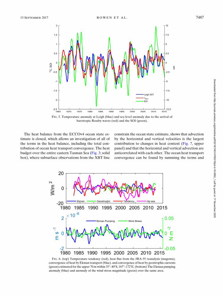
The temperature at Leigh is also compared to the
arrival of barotropic Rossby waves to examine poten-
tial connections between sea surface temperature and
ocean adjustment around New Zealand (Fig. 5). The
arrival of barotropic Rossby waves is highly correlated
with the Leigh temperatures (r5 0:64; p, 0:001) and
with the SOI (r5 0:55; p, 0:001). This correlation
suggests there may be a connection between the arrival
of barotropic waves and adjustment of the thermocline
around the country. However, an examination of the
heat balance is required to understand the role of each
term in the interannual temperature variations at Leigh
and the surrounding region (Fig. 3). Since Leigh is
adjacent to the strong East Auckland Current, we in-
vestigate the heat balance in the eastern Tasman Sea
where temperatures are highly correlated with those
at Leigh.
4. The upper ocean heat balance in the easternTasman Sea
We first examine the upper ocean heat balance di-
rectly fromobservations in a 58 3 58 region in the easternTasman Sea (358–408S, 1678–1728E; see dotted box in
Fig. 3). Terms in the heat budget of the upper 70m from
the observations show that temperature tendency and
air–sea heat flux are usually the largest terms and cor-
related with each other (Fig. 6, upper panel). Advection
of heat by Ekman and geostrophic currents are smaller.
As noted by Ummenhofer and England (2007), the
Ekman transport does not have the right phase to drive
the temperature changes. Local vertical velocities from
Ekman pumping, calculated from the wind stress curl,
are not clearly related to changes in temperature
(Fig. 6). Wind stress magnitude anomaly over the region
is not highly correlated with temperature tendency
(Fig. 6, lower panel), suggesting that wind-driven
changes in vertical mixing or latent heat flux are not
primarily responsible for the temperature changes.
Thus, from the terms that can be calculated directly from
observations, only the air–sea flux appears to be a likely
dominant driver.
FIG. 3. The correlation of the Leigh temperatures with satellite
SST over the period 1981 to 2015. The temperature time series have
had the seasonal cycle removed and are smoothed annually before
correlating. The box in the Tasman Sea is the region where the
upper-ocean heat balance is examined in the ocean state analysis.
The dotted lines show the region of the observational heat budget
analysis. The black dashed line shows the PX34 XBT line.
FIG. 4. Net surface heat flux over a 28 3 28 region around Leigh
from the JRA-55 reanalysis (red), the GECCO2 ocean state esti-
mate (light blue), the ECCOv4 ocean state estimate (green), and
the OAFlux project (magenta) are compared to the upper-ocean
heat content tendency estimated from the Leigh time series (blue).
Positive heat flux is into the ocean.
7486 JOURNAL OF CL IMATE VOLUME 30
Dow
nloaded from http://journals.am
etsoc.org/jcli/article-pdf/30/18/7481/4769319/jcli-d-16-0852_1.pdf by guest on 17 Novem
ber 2020
Page 7
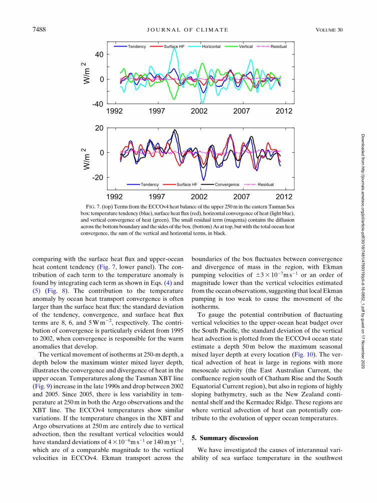
The heat balance from the ECCOv4 ocean state es-
timate is closed, which allows an investigation of all of
the terms in the heat balance, including the total con-
tribution of ocean heat transport convergence. The heat
budget over the entire eastern Tasman Sea (Fig. 3; solid
box), where subsurface observations from the XBT line
constrain the ocean state estimate, shows that advection
by the horizontal and vertical velocities is the largest
contribution to changes in heat content (Fig. 7, upper
panel) and that the horizontal and vertical advection are
anticorrelated with each other. The ocean heat transport
convergence can be found by summing the terms and
FIG. 6. (top) Temperature tendency (red), heat flux from the JRA-55 reanalysis (magenta),
convergence of heat by Ekman transport (blue), and convergence of heat by geostrophic currents
(green) estimated for the upper 70mwithin 358–408S, 1678–1728E. (bottom)TheEkmanpumping
anomaly (blue) and anomaly of the wind stress magnitude (green) over the same area.
FIG. 5. Temperature anomaly at Leigh (blue) and sea level anomaly due to the arrival of
barotropic Rossby waves (red) and the SOI (green).
15 SEPTEMBER 2017 BOWEN ET AL . 7487
Dow
nloaded from http://journals.am
etsoc.org/jcli/article-pdf/30/18/7481/4769319/jcli-d-16-0852_1.pdf by guest on 17 Novem
ber 2020
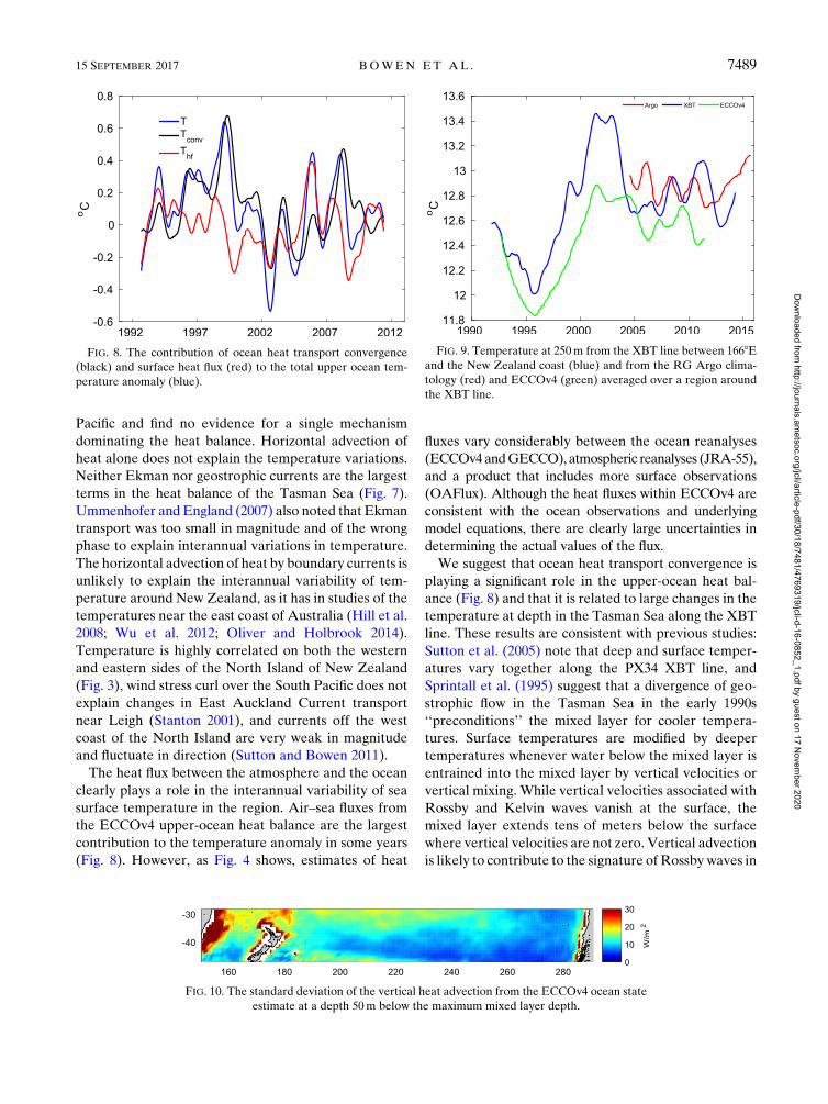
Page 8
comparing with the surface heat flux and upper-ocean
heat content tendency (Fig. 7, lower panel). The con-
tribution of each term to the temperature anomaly is
found by integrating each term as shown in Eqs. (4) and
(5) (Fig. 8). The contribution to the temperature
anomaly by ocean heat transport convergence is often
larger than the surface heat flux: the standard deviation
of the tendency, convergence, and surface heat flux
terms are 8, 6, and 5Wm22, respectively. The contri-
bution of convergence is particularly evident from 1995
to 2002, when convergence is responsible for the warm
anomalies that develop.
The vertical movement of isotherms at 250-m depth, a
depth below the maximum winter mixed layer depth,
illustrates the convergence and divergence of heat in the
upper ocean. Temperatures along the Tasman XBT line
(Fig. 9) increase in the late 1990s and drop between 2002
and 2005. Since 2005, there is less variability in tem-
perature at 250m in both the Argo observations and the
XBT line. The ECCOv4 temperatures show similar
variations. If the temperature changes in the XBT and
Argo observations at 250m are entirely due to vertical
advection, then the resultant vertical velocities would
have standard deviations of 431026m s21 or 140myr21,
which are of a comparable magnitude to the vertical
velocities in ECCOv4. Ekman transport across the
boundaries of the box fluctuates between convergence
and divergence of mass in the region, with Ekman
pumping velocities of 633 1027m s21 or an order of
magnitude lower than the vertical velocities estimated
from the ocean observations, suggesting that local Ekman
pumping is too weak to cause the movement of the
isotherms.
To gauge the potential contribution of fluctuating
vertical velocities to the upper-ocean heat budget over
the South Pacific, the standard deviation of the vertical
heat advection is plotted from the ECCOv4 ocean state
estimate a depth 50m below the maximum seasonal
mixed layer depth at every location (Fig. 10). The ver-
tical advection of heat is large in regions with more
mesoscale activity (the East Australian Current, the
confluence region south of Chatham Rise and the South
Equatorial Current region), but also in regions of highly
sloping bathymetry, such as the New Zealand conti-
nental shelf and the Kermadec Ridge. These regions are
where vertical advection of heat can potentially con-
tribute to the evolution of upper ocean temperatures.
5. Summary discussion
We have investigated the causes of interannual vari-
ability of sea surface temperature in the southwest
FIG. 7. (top) Terms from theECCOv4 heat balance of the upper 250m in the eastern Tasman Sea
box: temperature tendency (blue), surface heat flux (red), horizontal convergenceof heat (light blue),
and vertical convergence of heat (green). The small residual term (magenta) contains the diffusion
across the bottomboundary and the sides of thebox. (bottom)As at top, butwith the total oceanheat
convergence, the sum of the vertical and horizontal terms, in black.
7488 JOURNAL OF CL IMATE VOLUME 30
Dow
nloaded from http://journals.am
etsoc.org/jcli/article-pdf/30/18/7481/4769319/jcli-d-16-0852_1.pdf by guest on 17 Novem
ber 2020
Page 9
Pacific and find no evidence for a single mechanism
dominating the heat balance. Horizontal advection of
heat alone does not explain the temperature variations.
Neither Ekman nor geostrophic currents are the largest
terms in the heat balance of the Tasman Sea (Fig. 7).
Ummenhofer and England (2007) also noted that Ekman
transport was too small in magnitude and of the wrong
phase to explain interannual variations in temperature.
The horizontal advection of heat by boundary currents is
unlikely to explain the interannual variability of tem-
perature around New Zealand, as it has in studies of the
temperatures near the east coast of Australia (Hill et al.
2008; Wu et al. 2012; Oliver and Holbrook 2014).
Temperature is highly correlated on both the western
and eastern sides of the North Island of New Zealand
(Fig. 3), wind stress curl over the South Pacific does not
explain changes in East Auckland Current transport
near Leigh (Stanton 2001), and currents off the west
coast of the North Island are very weak in magnitude
and fluctuate in direction (Sutton and Bowen 2011).
The heat flux between the atmosphere and the ocean
clearly plays a role in the interannual variability of sea
surface temperature in the region. Air–sea fluxes from
the ECCOv4 upper-ocean heat balance are the largest
contribution to the temperature anomaly in some years
(Fig. 8). However, as Fig. 4 shows, estimates of heat
fluxes vary considerably between the ocean reanalyses
(ECCOv4andGECCO), atmospheric reanalyses (JRA-55),
and a product that includes more surface observations
(OAFlux). Although the heat fluxes within ECCOv4 are
consistent with the ocean observations and underlying
model equations, there are clearly large uncertainties in
determining the actual values of the flux.
We suggest that ocean heat transport convergence is
playing a significant role in the upper-ocean heat bal-
ance (Fig. 8) and that it is related to large changes in the
temperature at depth in the Tasman Sea along the XBT
line. These results are consistent with previous studies:
Sutton et al. (2005) note that deep and surface temper-
atures vary together along the PX34 XBT line, and
Sprintall et al. (1995) suggest that a divergence of geo-
strophic flow in the Tasman Sea in the early 1990s
‘‘preconditions’’ the mixed layer for cooler tempera-
tures. Surface temperatures are modified by deeper
temperatures whenever water below the mixed layer is
entrained into the mixed layer by vertical velocities or
vertical mixing. While vertical velocities associated with
Rossby and Kelvin waves vanish at the surface, the
mixed layer extends tens of meters below the surface
where vertical velocities are not zero. Vertical advection
is likely to contribute to the signature of Rossby waves in
FIG. 10. The standard deviation of the vertical heat advection from the ECCOv4 ocean state
estimate at a depth 50m below the maximum mixed layer depth.
FIG. 9. Temperature at 250m from the XBT line between 1668Eand the New Zealand coast (blue) and from the RG Argo clima-
tology (red) and ECCOv4 (green) averaged over a region around
the XBT line.
FIG. 8. The contribution of ocean heat transport convergence
(black) and surface heat flux (red) to the total upper ocean tem-
perature anomaly (blue).
15 SEPTEMBER 2017 BOWEN ET AL . 7489
Dow
nloaded from http://journals.am
etsoc.org/jcli/article-pdf/30/18/7481/4769319/jcli-d-16-0852_1.pdf by guest on 17 Novem
ber 2020
Page 10
ocean color observations by injecting nutrients into the
mixed layer (Charria et al. 2006) and may also contrib-
ute to propagating features in sea surface temperatures
observed in all the ocean basins (Hill et al. 2000).
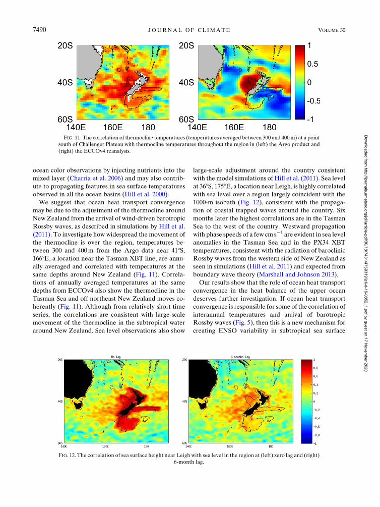
We suggest that ocean heat transport convergence
may be due to the adjustment of the thermocline around
New Zealand from the arrival of wind-driven barotropic
Rossby waves, as described in simulations by Hill et al.
(2011). To investigate how widespread the movement of
the thermocline is over the region, temperatures be-
tween 300 and 400m from the Argo data near 418S,1668E, a location near the Tasman XBT line, are annu-
ally averaged and correlated with temperatures at the
same depths around New Zealand (Fig. 11). Correla-
tions of annually averaged temperatures at the same
depths from ECCOv4 also show the thermocline in the
Tasman Sea and off northeast New Zealand moves co-
herently (Fig. 11). Although from relatively short time
series, the correlations are consistent with large-scale
movement of the thermocline in the subtropical water
around New Zealand. Sea level observations also show
large-scale adjustment around the country consistent
with the model simulations of Hill et al. (2011). Sea level
at 368S, 1758E, a location near Leigh, is highly correlated
with sea level over a region largely coincident with the
1000-m isobath (Fig. 12), consistent with the propaga-
tion of coastal trapped waves around the country. Six
months later the highest correlations are in the Tasman
Sea to the west of the country. Westward propagation
with phase speeds of a few cms21 are evident in sea level
anomalies in the Tasman Sea and in the PX34 XBT
temperatures, consistent with the radiation of baroclinic
Rossby waves from the western side of New Zealand as
seen in simulations (Hill et al. 2011) and expected from
boundary wave theory (Marshall and Johnson 2013).
Our results show that the role of ocean heat transport
convergence in the heat balance of the upper ocean
deserves further investigation. If ocean heat transport
convergence is responsible for some of the correlation of
interannual temperatures and arrival of barotropic
Rossby waves (Fig. 5), then this is a new mechanism for
creating ENSO variability in subtropical sea surface
FIG. 11. The correlation of thermocline temperatures (temperatures averaged between 300 and 400m) at a point
south of Challenger Plateau with thermocline temperatures throughout the region in (left) the Argo product and
(right) the ECCOv4 reanalysis.
FIG. 12. The correlation of sea surface height near Leigh with sea level in the region at (left) zero lag and (right)
6-month lag.
7490 JOURNAL OF CL IMATE VOLUME 30
Dow
nloaded from http://journals.am
etsoc.org/jcli/article-pdf/30/18/7481/4769319/jcli-d-16-0852_1.pdf by guest on 17 Novem
ber 2020
Page 11
temperatures, distinctly different from the ‘‘imprinting’’
of variability on the ocean by the atmosphere through
air–sea heat flux that has been the focus of previous
studies (e.g., Ciasto and England 2011; Fauchereau et al.
2003). Ocean heat transport convergence would also
contribute to ENSO variability in the fluxes of sensible
and latent heat between the ocean and the atmosphere.
Quantifying the movement of heat between the upper
ocean and deeper ocean will be critical to future un-
derstanding of interannual sea surface temperature
variability.
Acknowledgments. We thank Estimating the Circu-
lation and Climate of the Ocean (ECCO) Consortium
for providing the ECCOv4 product, which can be
downloaded from ftp://mit.ecco-group.org/ecco_for_las/
version_4/release1/. TheGECCO2 produced is from the
Integrated ClimateData Center, University of Hamburg.
The JRA-55 atmospheric reanalyses are available
from http://rda.ucar.edu/datasets/ds628.0/. The OISST is
available from http://www.esrl.noaa.gov/psd/data/gridded/
data.noaa.oisst.v2.html. The Roemmich and Gilson
climatology is available from http://sio-argo.ucsd.edu/
RG_Climatology.html. Temperatures from the XBT
lines in the Tasman Sea are available at http://www-hrx.
ucsd.edu/index.html. The NZT7 anomalies are available
from NIWA (https://www.niwa.co.nz/our-science/climate/
information-and-resources/nz-temp-record/seven-station-
series-temperature-data). Sea surface height and geo-
strophic velocities are available fromAVISO (http://www.
aviso.altimetry.fr/en/home.html). Leigh temperatures are
available from the authors on request.
M.B. and P.S. were partially supported by the New
Zealand Deep South National Science Challenge. J.M.
would like to acknowledge support from the
Friends of Leigh scholarship. X.Z. was supported by
the Earth System and Climate Change Hub of the
Australian Government’s National Environmental
Science Programme.
The authors thank three anonymous reviewers for
constructive comments that greatly improved the
manuscript.
REFERENCES
Bowen, M. M., P. J. H. Sutton, and D. Roemmich, 2006: Wind-
driven and steric fluctuations of sea surface height in the
southwest Pacific. Geophys. Res. Lett., 33, L14617,
doi:10.1029/2006GL026160.
Charria, G., I. Dadou, P. Cipollini, M. Drévillon, P. De Mey, and
V. Garçon, 2006: Understanding the influence of Rossby
waves on surface chlorophyll concentrations in the North
Atlantic Ocean. J. Mar. Res., 64, 43–71, doi:10.1357/
002224006776412340.
Ciasto, L. M., and D. W. J. Thompson, 2009: Observational
evidence of reemergence in the extratropical Southern
Hemisphere. J. Climate, 22, 1446–1453, doi:10.1175/
2008JCLI2545.1.
——, and M. H. England, 2011: Observed ENSO teleconnections
to Southern Ocean SST anomalies diagnosed from a surface
mixed layer heat budget. Geophys. Res. Lett., 38, L09701,
doi:10.1029/2011GL046895.
de Boyer Montgut, C., G. Madec, A. S. Fischer, A. Lazar, and
D. Iudicone, 2004: Mixed layer depth over the global ocean:
An examination of profile data and a profile-based climatol-
ogy. J. Geophys. Res., 109, C12003, doi:10.1029/2004JC002378.
Deser, C.,M.A.Alexander, andM. S. Timlin, 2003:Understanding the
persistence of sea surface temperature anomalies in midlatitudes.
J. Climate, 16, 57–72, doi:10.1175/1520-0442(2003)016,0057:
UTPOSS.2.0.CO;2.
——, ——, S.-P. Xie, and A. S. Phillips, 2010: Sea surface temper-
ature variability: Patterns and mechanisms. Annu. Rev. Mar.
Sci., 2, 115–143, doi:10.1146/annurev-marine-120408-151453.
Ducet, N., and P. Y. LeTraon, 2000: Global high-resolution map-
ping of ocean circulation from TOPEX/Poseidon and ERS-1
and -2. J. Geophys. Res., 105, 19 477–19 498, doi:10.1029/
2000JC900063.
Emery, W. J., and R. E. Thomson, 2001: Data Analysis Methods in
Physical Oceanography. Elsevier, 654 pp.
Evans, J., and J. Atkins, 2008: Seawater temperature dataset at
Goat Island, Leigh, New Zealand from 1967 to 2011. Uni-
versity of Auckland. [Available online at https://hdl.handle.
net/2292/20612.]
Fauchereau, N., S. Trzaska, Y. Richard, P. Roucou, and
P. Camberlin, 2003: Sea-surface temperature co-variability in
the southern Atlantic and Indian Oceans and its connections
with the atmospheric circulation in the Southern Hemisphere.
Int. J. Climatol., 23, 663–677, doi:10.1002/joc.905.
Folland, C., and M. Salinger, 1995: Surface temperature trends
and variations in New Zealand and the surrounding ocean,
1871–1993. Int. J. Climatol., 15, 1195–1218, doi:10.1002/
joc.3370151103.
Forget, G., J.-M. Campin, P. Heimbach, C. N. Hill, R. M. Ponte,
and C. Wunsch, 2015: ECCO version 4: An integrated
framework for non-linear inverse modeling and global ocean
state estimation. Geosci. Model Dev., 8, 3071–3104,
doi:10.5194/gmd-8-3071-2015.
Frankignoul, C., P. Müller, and E. Zorita, 1997: A simple model
of the decadal response of the ocean to stochastic wind
forcing. J. Phys. Oceanogr., 27, 1533–1546, doi:10.1175/
1520-0485(1997)027,1533:ASMOTD.2.0.CO;2.
Godfrey, J. S., 1989: A Sverdrup model of the depth-integrated
flow for the world ocean allowing for island circulations. Geo-
phys. Astrophys. Fluid Dyn., 45, 89–112, doi:10.1080/
03091928908208894.
Greig,M., N.M.Ridgway, andB. S. Shakespeare, 1988: Sea surface
temperature variations at coastal sites around New Zealand.
N. Z. J. Mar. Freshwater Res., 22, 391–400, doi:10.1080/
00288330.1988.9516310.
Guan, Y., B. Huang, J. Zhu, Z.-Z. Hu, and J. L. Kinter, 2014: In-
terannual variability of the South Pacific Ocean in observations
and simulated by the NCEP Climate Forecast System, version
2. Climate Dyn., 43, 1141–1157, doi:10.1007/s00382-014-2148-y.
Hill, K. L., I. S. Robinson, and P. Cipollini, 2000: Propagation
characteristics of extratropical planetary waves observed in
the ATSR global sea surface temperature record. J. Geophys.
Res., 105, 21 927–21 945, doi:10.1029/2000JC900067.
15 SEPTEMBER 2017 BOWEN ET AL . 7491
Dow
nloaded from http://journals.am
etsoc.org/jcli/article-pdf/30/18/7481/4769319/jcli-d-16-0852_1.pdf by guest on 17 Novem
ber 2020
Page 12
——, S. R. Rintoul, R. Coleman, and K. R. Ridgway, 2008: Wind
forced low frequency variability of the East Australian Cur-
rent. Geophys. Res. Lett., 35, L08602, doi:10.1029/
2007GL032912.
——, ——, K. Ridgway, and P. R. Oke, 2011: Decadal changes in
the South Pacific western boundary current system revealed in
observations and ocean state estimates. J. Geophys. Res., 116,
C01009, doi:10.1029/2009JC005926.
Holbrook, N. J., and N. L. Bindoff, 1997: Interannual and decadal
temperature variability in the southwest Pacific Ocean be-
tween 1955 and 1988. J. Climate, 10, 1035–1049, doi:10.1175/
1520-0442(1997)010,1035:IADTVI.2.0.CO;2.
Kobayashi, S., and Coauthors, 2015: The JRA-55 Reanalysis:
General specification and basic characteristics. J. Meteor. Soc.
Japan, 93, 5–48, doi:10.2151/jmsj.2015-001.
Köhl, A., 2015: Evaluation of the GECCO2 ocean synthesis:
Transports of volume, heat and freshwater in the Atlantic.
Quart. J. Roy. Meteor. Soc., 141, 166–181, doi:10.1002/qj.2347.
Marshall, D. P., and H. L. Johnson, 2013: Propagation of merid-
ional circulation anomalies along western and eastern
boundaries. J. Phys. Oceanogr., 43, 2699–2717, doi:10.1175/
JPO-D-13-0134.1.
Mullan, A. B., S. J. Stuart, M. G. Hadfield, andM. J. Smith, 2010:
Report on the review of NIWA’s ‘Seven-Station’ tempera-
ture series. Tech. Rep. NIWA Information Series 78,
175 pp.
Oliver, E. C. J., and N. J. Holbrook, 2014: Extending our un-
derstanding of South Pacific gyre ‘‘spin-up’’: Modeling the
East Australian Current in a future climate. J. Geophys. Res.
Oceans, 119, 2788–2805, doi:10.1002/2013JC009591.Reynolds, R. W., N. A. Rayner, T. M. Smith, D. C. Stokes, and
W. Wang, 2002: An improved in situ and satellite SST anal-
ysis for climate. J. Climate, 15, 1609–1625, doi:10.1175/
1520-0442(2002)015,1609:AIISAS.2.0.CO;2.
Rintoul, S. R., and M. H. England, 2002: Ekman transport domi-
nates local air–sea fluxes in driving variability of subantarctic
mode water. J. Phys. Oceanogr., 32, 1308–1321, doi:10.1175/1520-0485(2002)032,1308:ETDLAS.2.0.CO;2.
Roberts, C. D., M. D. Palmer, R. P. Allan, D. G. Desbruyeres,
P. Hyder, C. Liu, and D. Smith, 2017: Surface flux and ocean
heat transport convergence contributions to seasonal and in-
terannual variations of ocean heat content. J. Geophys. Res.,
122, 726–744, doi:10.1002/2016JC012278.
Roemmich, D., and J. Gilson, 2009: The 2004–2008 mean and an-
nual cycle of temperature, salinity, and steric height in the
global ocean from theArgo Program.Prog. Oceanogr., 82, 81–
100, doi:10.1016/j.pocean.2009.03.004.
Sasaki, Y. N., S.Minobe, N. Schneider, T. Kagimoto,M.Nonaka, and
H. Sasaki, 2008: Decadal sea level variability in the South Pacific
in a global eddy-resolving ocean model hindcast. J. Phys. Oce-
anogr., 38, 1731–1747, doi:10.1175/2007JPO3915.1.
Sharples, J., 1997: Cross-shelf intrusion of subtropical water into
the coastal zone of northeast New Zealand. Cont. Shelf Res.,
17, 835–857, doi:10.1016/S0278-4343(96)00060-X.
Sprintall, J., D. Roemmich, B. Stanton, and R. Bailey, 1995: Re-
gional climate variability and ocean heat transport in the
southwest Pacific Ocean. J. Geophys. Res., 100, 15 865–15 871,
doi:10.1029/95JC01664.
Stanton, B. R., 2001: Estimating the East Auckland Current
transport from model winds and the Island Rule. N. Z.
J. Mar. Freshwater Res., 35, 531–540, doi:10.1080/
00288330.2001.9517020.
Sutton, P. J. H., andM.M. Bowen, 2011: Currents off the west coast
of Northland, New Zealand.N. Z. J. Mar. Freshwater Res., 45,
609–624, doi:10.1080/00288330.2011.569729.
——,——, andD. Roemmich, 2005: Decadal temperature changes
in the Tasman Sea. N. Z. J. Mar. Freshwater Res., 39, 1321–
1329, doi:10.1080/00288330.2005.9517396.
Ummenhofer, C., and M. H. England, 2007: Interannual extremes
in New Zealand precipitation linked to modes of Southern
Hemisphere climate variability. J. Climate, 20, 5418–5440,
doi:10.1175/2007JCLI1430.1.
Verdy, A., J. Marshall, and A. Czaja, 2006: Sea surface temperature
variability along the path of theAntarcticCircumpolar Current.
J. Phys. Oceanogr., 36, 1317–1331, doi:10.1175/JPO2913.1.
Wu, L., and Coauthors, 2012: Enhanced warming over the global
subtropical western boundary currents. Nat. Climate Change,
2, 161–166, doi:10.1038/nclimate1353.
Yu, L., and R. A. Weller, 2007: Objectively analyzed air–sea heat
fluxes for the global ice-free oceans (1981–2005). Bull. Amer.
Meteor. Soc., 88, 527–539, doi:10.1175/BAMS-88-4-527.
Zeldis, J. R., R. A. Walters, M. J. N. Greig, and K. Image, 2004:
Circulation over the northeastern New Zealand continen-
tal slope, shelf and adjacent Hauraki Gulf, during spring
and summer. Cont. Shelf Res., 24, 543–561, doi:10.1016/
j.csr.2003.11.007.
7492 JOURNAL OF CL IMATE VOLUME 30
Dow
nloaded from http://journals.am
etsoc.org/jcli/article-pdf/30/18/7481/4769319/jcli-d-16-0852_1.pdf by guest on 17 Novem
ber 2020