Interconnect Delay Models

Basic Circuit Analysis Techniques

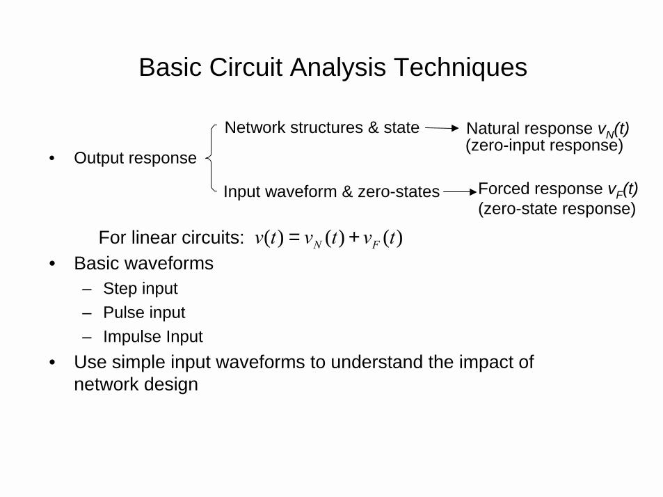
• Output response

• Basic waveforms– Step input– Pulse input– Impulse Input

• Use simple input waveforms to understand the impact of network design

Network structures & state

Input waveform & zero-states

Natural response vN(t)(zero-input response)

Forced response vF(t)(zero-state response)

For linear circuits: )()()( tvtvtv FN +=

unit step function

u(t)=0

1

0<t

0≥t

1

pulse function of width T

0

1/T

-T/2 T/2

−−+= )

2()

2(1)( TtuTtu

TtPT

unit impulse function

∫− =

>=≠=

→

ζ

ζδ

ζ

δδ

1)(

0any for s.t.0for singular 0for 0)(

0when )( : )(

dtt

ttt

TtPt T

dttduδ(t)

dxxtut

)(or

)()(

definitionBy

=

= ∫ ∞−δ

Basic Input Waveforms

• Definitions:– (unit) step input u(t) (unit) step response g(t)– (unit) impulse input δ(t) (unit) impulse response h(t)

• Relationship

• Elmore delay

∫∫ =→=

=→=

∞−

ttdxxhtgdxxtu

dttdgth

dttdut

0)()()()(

)()()()(

δ

δ

Step Response vs. Impulse Response

(Input Waveform) (Output Waveform)

∫ ∫∞ ∞

⋅=⋅=0 0

)()(' dttthdtttgTD

Analysis of Simple RC Circuit

)()()(

)())(()(

)()()(

tvtvdt

tdvRC

dttdvC

dttCvdti

tvtvtiR

T

T

=+⇒

==

=+⋅

first-order linear differentialequation with

constant coefficients

state variable

Inputwaveform

±v(t)C

RvT(t)

i(t)

Analysis of Simple RC Circuit

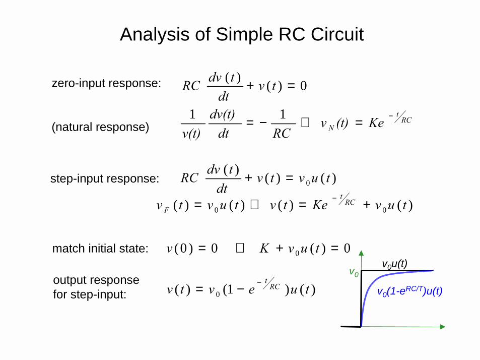
0)()( =+ tvdt

tdvRCzero-input response:

(natural response)

step-input response:

match initial state:

output responsefor step-input:

v0v0u(t)

v0(1-eRC/T)u(t)

RCt

N Ke(t)vRCdt

dv(t)v(t)

−=⇒−= 11

)()()(0 tuvtv

dttdvRC =+

)()()()( 00 tuvKetvtuvtv RCt

F +=⇒= −

)()1()( 0 tuevtv RCt−−=

0)( 0)0( 0 =+⇒= tuvKv

Delays of Simple RC Circuit

• v(t) = v0(1 - e-t/RC) under step input v0u(t)

• v(t)=0.9v0 ⇒ t = 2.3RCv(t)=0.5v0 ⇒ t = 0.7RC

• Commonly used metricTD = RC (Elmore delay to be defined later)

Lumped Capacitance Delay Model• R = driver resistance• C = total interconnect capacitance + loading capacitance• Sink Delay: td = R·C

• 50% delay under step input = 0.7RC• Valid when driver resistance >> interconnect resistance• All sinks have equal delay

driver

3N

2N

+N

Rd

Cload

( )( )g0d

gintdloaddD

CLCRCCRCRt

+⋅⋅=

+⋅=⋅=

driver

3N

2N

+N

Lumped RC Delay Model

• Minimize delay ⇔ minimize wire length

Rd

Cload

Delay of Distributed RC Lines

......!4!2

1

2)cosh(

cosh1)(

42

+++=

+=

=

−

xx

eex

sRCssV

xx

out

Vout(t) Vout(s)LaplaceTransform

RVIN VOUT

CVOUTVIN

R

C

0.5

1.0

VOUT

DISTRIBUTED

LUMPED

1.0RC 2.0RC time

Step response of distributed and lumped RC networks.A potential step is applied at VIN, and the resulting VOUTis plotted. The time delays between commonly usedreference points in the output potential is also tabulated.

Delay of Distributed RC Lines (cont’d)

Output potential range Time elapsed(Distributed RC

Network)

Time elapsed(Lumped RC

Network)0 to 90% 1.0 RC 2.3 RC

10% to 90% (rise time) 0.9 RC 2.2 RC

0 to 63% 0.5 RC 1.0 RC

0 to 50% (delay) 0.4 RC 0.7 RC

0 to 10% 0.1 RC 0.1 RC

Distributed Interconnect Models

• Distributed RC circuit model– L,T or Π circuits

• Distributed RCL circuit model

• Tree of transmission lines

Distributed RC Circuit Models

0Z

0Z

Distributed RLC Circuit Model

Delays of Complex Circuits under Unit Step Input

• Circuits with monotonic response

• Easy to define delay & rise/fall time• Commonly used definitions

– Delay T50% = time to reach half-value, v(T50%) = 0.5Vdd

– Rise/fall time TR = 1/v’(T50%) where v’(t): rate of change of v(t)w.r.t. t

– Or rise time = time from 10% to 90% of final value• Problem: lack of general analytical formula for T50% &

TR!

t

10.5

v(t)T50%

TR

t

Delays of Complex Circuits under Unit Step Input (cont’d)

• Circuits with non-monotonic response

• Much more difficult to define delay & rise/fall time

)( of change of rate : )('(monotone) responseoutput : )(

tvtvtv

0.5

1

T50%

v(t)

t

t

v�(t)

medianof v�(t)(T50%) v'(t)

dtttvTD

ofmean

)('0∫∞

=

Elmore Delay for Monotonic Responses

• Assumptions:– Unit step input – Monotone output response

• Basic idea: use of mean of v’(t) to approximate median of v’(t)

• T50%: median of v’(t), since

• Elmore delay TD = mean of v’(t)

def.)(by )( of valuefinal of half

)(')('%50

%500

tv

dttvdttvT

T

=

=∫ ∫+∞

∫∞

=0

)(' tdttvT D

Elmore Delay for Monotonic Responses

Why Elmore Delay?

• Elmore delay is easier to compute analytically in most cases– Elmore’s insight [Elmore, J. App. Phy 1948]– Verified later on by many other researchers, e.g.

• Elmore delay for RC trees [Penfield-Rubinstein, DAC’81]• Elmore delay for RC networks with ramp input [Chan, T-

CAS’86]• .....

• For RC trees: [Krauter-Tatuianu-Willis-Pileggi, DAC’95]T50% ≤ TD

• Note: Elmore delay is not 50% value delay in general!

Elmore Delay for RC Trees

• Definition– h(t) = impulse response– TD = mean of h(t)

=

• Interpretation– H(t) = output response (step process)– h(t) = rate of change of H(t)– T50%= median of h(t)– Elmore delay approximates the median of h(t) by

the mean of h(t)

∫∞

⋅0

dtt h(t)

medianof v�(t)(T50%) v'(t)

dtttvTD

ofmean

)('0∫∞

=

h(t) = impulse response

H(t) = step response

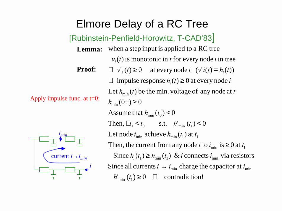
Elmore Delay of a RC Tree[Rubinstein-Penfield-Horowitz, T-CAD’83]

ion!contradict 0)(' at capacitor thecharge currents all Since

resistors via connects & )()( Since at 0 is to nodeany fromcurrent theThen,

at )( achieve nodeLet 0)(' s.t. Then,

0)( that Assume0)0(

at nodeany of voltagemin. thebe )(Let nodeevery at 0)( response impulse

))()('( nodeevery at 0)(' in tree nodeevery for in monotonic is )(

treeRC a toapplied isinput step awhen

1min

minmin

min1min1

1min

11minmin

1min01

0min

min

min

⇒≥→

≥≥

<<∃<

≥+

≥⇔=≥⇔

thiii

iiththtii

tthithtt

thh

tthith

thtivitvittv

i

i

ii

i

Lemma:

Proof:

Apply impulse func. at t=0:

imin

icurrent i→imin

Elmore Delay in a RC Tree (cont’d)

∫∫∫∫

∑∑

∑

∑

∑

∞

∞→∞→

∞∞∞

∈

−+⋅−=−⋅=

−⋅=⋅=

=⋅=

⋅=

⋅==−

=

=

∩

00

000

i

))(1()1)((lim])()([lim

)(|)()('

)()(

) and between res.path (common ) cap o(current t

)in scap' all current to(on drop voltageThe)(1

)( node of cap. current to The

node delay to Elmore

& input to from

pathcommon of resistance: at rooted subtree: ; node input to frompath :

dttvTTvdttvTTv

dttvttvdtttvT

dttdvCRR

dttdvC

PPk

SRPtvdt

tdvCi

CRTi

kjPPR

isiP

iiT

T

iiT

iiiD

k

kkkiki

k

kk

kki

Pkikii

i

kkkiD

kj

jk

ii

i

i

i

inputi

k

jSi

path resistance Rii

Rjk

Theorem :

Proof :

Elmore Delay in a RC Tree (cont’d)• We shall show later on that

i.e. 1-vi(T) goes to 0 at a much faster rate than 1/T when T→∞

• Let

0))(1(lim =⋅−∞→

TTviT

)(

)](1[))(1(lim

)(

)](1[

)(

)()(

)](1[)(

0

0

0

∑∫

∑∑ ∑∑∫ ∑

∫

=∞=

−+−=∴

=∞

−−=

=

=

−=

∞

∞→

kkkii

iiTD

kkkii

k kkkkikki

kkkki

t

k

kkkii

t

ii

CRf

dttvTTvT

CRf

tvCRCR

tvCR

dxdx

xdvCRtf

dxxvtf

i

(1)

vi(t)

1

0 t

area ∫ −=t

ii dxxvtf0

)](1[)(

) & (since Then,

)(

Recall Let

2

kiiikikkpDR

iik

kkiR

kkkiD

kkkkp

RRRRTTT

RCRT

CRTCRT

ii

i

i

≥≥≤≤

=

==

∑∑∑

Some Definitions For Signal Bound Computation

Signal Bounds in RC Trees• Theorem

ii

iRiRiRiD

i

i

i

ppRip

i

ii

i

RDT

tT

TT

p

R

i

p

D

RpT

tT

TT

p

D

RDRi

Di

TTteeTT

tv

tT

tT

TTteeTT

TTttTt

Ttv

t

−≥⋅−

≤

≥−

−

−≥⋅−

−≥≥+

−≥

≥

−−

−−

)(

)(

1

)(

0 1

bounds Upper

1

) when trivial-(non 0 1 )(

0 0 bounds Lower

Proofs of Signal Bounds in RC Trees• Lemma:

• Lemma:

monotonic) is )( (Since

0 )(

)(

)()()](1[)](1[

),min( ),max(

)](1[)](1[

tvdt

tdvCRRRR

dttdv

CRRdt

tdvCRR

tvRtvRRRRR

RRRRRR

tvRtvR

j

j

jjjikijkii

j j

jjjiki

jjjkii

ikikii

jikijkii

jikijkjikiii

ikikii

≥−=

−=

−−−

⋅≥⋅∴

≥≥

−≥−

∑

∑ ∑

Proof:(2)

)](1[)](1[ tvRtvR ikkkki −≤− (3)

Proofs of Signal Lower Bounds in RC Trees

ttvtfttttftftvtt

tv

etfTtfT

e

Tt(ttfTT

t(ttt

Tdttdf

tfTT

TtfT

dttdftv

TtfT

tvTtfTtvT

tvCRtfT

ii

iii

i

Ttt

iD

iDTtt

R

ttiD

p

R

i

iDp

R

iDii

p

iD

ipiDiR

kkkkiiD

iR

i

ip

ii

ii

i

ii

ii

i

⋅−≥==−≤−−

≥−−

≥

−≤−−≤−

≤⋅−

≤

−≤=−≤

−

−≤−≤−

−=−

−−−−

∑

)](1[)( ,0Let )()()](1)[(

monotonic is )( since Also,

)()(

i.e.

)|))(ln() : to from gIntegratin

1)()(

11 Thus,

)()()(1)(

i.e.

)](1[)()](1[ :(3) & (2) From

))(1()( :(1) From

43

34434

)(

1

2)(

121221

1212

2

1

fi(t4)-fi(t3)

(t4-t3)[1-vi(t4)]

t3 t4

(4)

(5)

(7)(6)

Proofs of Signal Lower Bounds in RC Trees

ppiRp

ipi

p

i

ii

p

ii

i

i

i

i

i

i

iii

Tt

TTT

p

DTt

p

Di

Tt

Dip

iDiR

Tt

DiD

iiiRp

Rp

R

Di

R

Di

iDiDiR

eeTT

eTT

tv

eTtvT

tfT(t)vT

eTtfT

ttt

tftftvTTttTTtt

TtT

tvTt

Ttv

ttvTtfTtvT

−−−−

−

−

⋅−=−≥∴

≤−

++

−≤−

≤−

==

−≤−−

=+−=

+−≥∴

+≤−⇒

−−≤−≤−

)(

3

321

3

43

11)(

)](1[

:)10()9()8(

)(]1[ (4) of half-left From

)(

(5) of half-leftin and 0Let

)()()](1)[(

(6)in Let

1)( )(1

)](1[)()](1[ (7) and (4) of half-left From

3

3

3

(8)

(9)

(10)

Delay Bounds in RC Trees

[ ]

[ ]

[ ] p

Di

ip

DipRp

Ri

D

p

Ri

ip

RRRD

ip

TT

tvtvT

TTTTt

Ttv

Tt

TT

tvtvT

TTTTt

tvTTt

i

i

i

i

ii

iii

−≥−

+−≤

−−

≤

−≥−

+−≥

−−≥

1)( when )(1

ln

)(1

:boundsUpper

1)(hen w)(1

ln

)(1:boundsLower

iD

Computation of Elmore Delay & Delay Bounds in RC Trees

• Let C(Tk) be total capacitance of subtree rooted at k• Elmore delay

fashion up-bottom ain y recursivel elinear timin computed becan formula threeall *

:boundlower

)( :boundupper

)(

2∑

∑

∑

⋅=

⋅=

⋅=∈

k ii

kkiR

kkkp

pkkkD

RCRT

TCRT

TCRT

i

i

i

Comments on Elmore Delay Model

• Advantages– Simple closed-form expression

• Useful for interconnect optimization– Upper bound of 50% delay [Gupta et al., DAC’95, TCAD’97]

• Actual delay asymptotically approaches Elmore delay as input signal rise time increases

– High fidelity [Boese et al., ICCD’93],[Cong-He, TODAES’96]• Good solutions under Elmore delay are good solutions under

actual (SPICE) delay

Comments on Elmore Delay Model

• Disadvantages– Low accuracy, especially poor for slope computation– Inherently cannot handle inductance effect

• Elmore delay is first moment of impulse response• Need higher order moments