1 Interest Rate and Investment under Uncertainty: Evidence from Commercial Real Estate Capital Improvements Liang Peng Leeds School of Business University of Colorado at Boulder Email: [email protected]Thomas G. Thibodeau Leeds School of Business University of Colorado at Boulder Email: [email protected]Abstract This paper empirically analyzes the non-monotonic influence that interest rate changes have on irreversible investment in income producing properties. Using the complete history of quarterly capital improvements for 1,416 commercial properties over the 1978 to 2009 period, we find strong evidence of the non-monotonic effect for apartment, office, and retail properties, but not for industrial properties. For the first three property types, a decrease in the Treasury yield dramatically increases capital improvements when property values are high, but has a weak or negative effect when property values are low. This result has important implications for monetary and fiscal policies. JEL classification: E22, E52 Key words: interest rate, investment under uncertainty, commercial real estate The authors thank the Real Estate Research Institute for a research grant and thank Marc Louargand and David Watkins for valuable comments. Liang Peng thanks the National Council of Real Estate Investment Fiduciaries (NCREIF) for providing the data. The authors take responsibility for any errors in this manuscript.
Transcript
1
Interest Rate and Investment under Uncertainty: Evidence from Commercial
This paper empirically analyzes the non-monotonic influence that interest rate changes have on irreversible investment in income producing properties. Using the complete history of quarterly capital improvements for 1,416 commercial properties over the 1978 to 2009 period, we find strong evidence of the non-monotonic effect for apartment, office, and retail properties, but not for industrial properties. For the first three property types, a decrease in the Treasury yield dramatically increases capital improvements when property values are high, but has a weak or negative effect when property values are low. This result has important implications for monetary and fiscal policies. JEL classification: E22, E52 Key words: interest rate, investment under uncertainty, commercial real estate
The authors thank the Real Estate Research Institute for a research grant and thank Marc Louargand and David Watkins for valuable comments. Liang Peng thanks the National Council of Real Estate Investment Fiduciaries (NCREIF) for providing the data. The authors take responsibility for any errors in this manuscript.
1
I. Introduction
Investment under uncertainty is one of the most important economic decisions that investors
make (e.g. Dixit and Pindyck (1994)). Among all variables that might affect investment, interest
rate changes have important implications for monetary and fiscal policies, and have drawn a lot
of attention from economists. While the neoclassical theory of investment (e.g. Jorgenson
(1963)) predicts that a decrease in the interest rate increases investment by reducing the cost of
capital, recent theoretical analyses (e.g. Capozza and Li (1994), Capozza and Li (2002), and
Chetty (2007)) suggest that, when firms make irreversible investments with uncertain pay-offs,
the effect of an interest rate change on investment is non-monotonic. Chetty (2007) specifically
suggests that investment is a backward-bending function of the interest rate. This means that a
decrease in the interest rate reduces investment when the interest rate is “low”, in the sense that
the difference between the interest rate and the expected future income growth rate is small, and
increases investment when the interest rate is “high”. While focusing on empirical analyses,
Capozza and Li (2001) also show that the difference between the discount rate and the expected
future income growth rate influences the investment responses to interest rate changes.
We empirically analyze the non-monotonic effect of interest rate changes on irreversible
investment using a unique dataset of individual capital improvements of 1,416 large commercial
properties, including apartment, office, industrial and retail properties, in a sample period from
1978 to 2009. In our empirical model, the non-monotonic effect is captured by an interaction
term between the change in the interest rate and the capitalization rate of properties. The
capitalization rate, which is also called the cap rate by real estate professionals, equals the ratio
of net operating income (NOI) to the property value. Real estate professionals conventionally
use the cap rate as a measurement of the valuation of properties: a low (high) cap rate indicates
high (low) property valuation. We show that, under reasonable assumptions, the cap rate
measures the difference between the cost of capital and the expected future income growth rate.
Therefore, the theory by Chetty (2007) predicts that a decrease in the interest rate increases
(reduces) the capital improvement when the cap rate is low (high).
We find strong evidence for the non-monotonic effect of interest rate changes on the capital
improvements in apartment, office, and retail properties, but not for industrial properties. For the
first three types of properties, a decrease in the Treasury yield dramatically increases
2
expenditures on capital improvements when property values are high (low cap rates), but has
little or negative effect when properties have low valuation (high cap rates). For example, when
the cap rate is 4%, a decrease of 50 basis points in the Treasury yield increases the capital
improvement by 18% for apartments, 15% for offices, and 31% for retail properties, but the same
interest rate decrease has no or negative effect when the cap rate is 10%. This result indicates
that a decrease in the interest rate may strongly stimulate investment in a booming economy
when asset values are high, but will have no or negative effect on investment in a recession when
assets values are low. This result has important policy implications. If a decrease in the interest
rate does not necessarily stimulate investment, then monetary authorities should take extreme
care when they try to use interest rate changes to stimulate investment.
The empirical evidence described above is novel. In fact, the existing literature provides little
empirical evidence regarding the non-monotonic effect of interest rate changes on investment.
The only empirical analysis prior to this paper is Capozza and Li (2001), which, however, differs
from this paper in research questions, data, method, and findings. For example, Capozza and Li
(2001) empirically analyze and substantiate the effect of the population growth rate and its
uncertainty on the likelihood of positive investment response to interest rate changes, while we
analyze and provide direct evidence that investment is a backward bending function of the
interest rate. Overall, the finding in this paper that the investment effect of interest rate changes
is related to asset valuation is original, has important policy implications, and makes an
important contribution to the literature.
The novel empirical evidence in this paper is made possible by the unique and high quality
dataset employed, which has a few important advantages. First, the real estate market is an ideal
environment to analyze investment under uncertainty, since real estate investments, including
capital improvements and development, are not only irreversible but also affected by real options
(e.g. Williams (1997)). Second, the dataset contains accurate measurements of both the timing
and the amount of capital improvements at the property level over the entire investment period
of each property. Property level data, or firm level data in a non-real estate environment, are
desirable for testing investment theories but are rarely available. Many researchers, including
Guiso and Parigi (1999), argue that property or firm level data are superior to aggregate data in
testing investment theories because investment decisions are made at the firm/property level.
3
Third, the sample period of the data is 30 years. This period covers several economic cycles and
provides valuable opportunities to observe dramatic changes in interest rates, which makes the
empirical tests in this paper powerful. Finally, the dataset contains accurate information on the
net operating income and owners’ appraised property values, which allows the calculation of the
cap rate and thus facilitates the measurement of property owners’ expectation of future income
growth. While investors’ expectation is an important variable that affects investment, it is rarely
observed in empirical research, with Guiso and Parigi (1999) being a notable exception.
The rest of this paper is organized as follows. Section II reviews the literature. Section III
discusses the empirical model. Section IV describes the data. Section V presents empirical
results, and section VI concludes.
II. Literature review
Pindyck (1991), Dixit and Pindyck (1994), Trigeorgis (1996), and Schwartz and Trigeorgis
(2001) provide good summaries of theoretical and empirical analyses on irreversible investment
under uncertainty. Below we briefly review more recent literature, which focuses more on real
option-based theories, the relationship between the cost of capital and investment, and the
influence of market structure on investment.
On the theory side, recent contributions to this literature include Grenadier (2002), Wang and
Zhou (2006), Novy-Marx (2007), and Chetty (2007). Grenadier (2002) demonstrates that
competition reduces the value of an investor’s real option and consequently increases investment.
Novy-Marx (2007) shows that, even in competitive markets, as long as products and opportunity
costs are heterogeneous, the option to delay can be valuable and thus investment can be lumpy.
Wang and Zhou (2006) demonstrate that the value of real options depend on market structure
(e.g. competitive, monopolistic, etc.). Chetty (2007) shows that a change in the interest rate
affects not only the net present values (NPVs) of possible projects but also the value of waiting.
More importantly, the effect on the value of waiting is stronger (weaker) than the effect on the
NPVs when the interest rate is “low” (“high”).1 Therefore, a decrease in the interest rate reduces
1 The “low” and “high” is defined according to the difference between the interest rate and the expected future income growth rate. An interest rate is “low” if the difference is small.
4
investment when the interest rate is low, but increases investment when the interest rate is high.
This non-monotonic effect of interest rates on investment is the main hypothesis of this paper.
On the empirical side, many recent analyses focus on non-real estate industries. For example,
Leahy and Whited (1996) use a panel of 772 manufacturing firms over the 1981 to 1987 period
to examine the response of investment to uncertainty. They demonstrate that firms postpone
investments when the uncertainty of the payoff increases. Guiso and Parigi (1999) use cross-
sectional data for 549 Italian manufacturing firms to examine whether uncertainty in future
expected benefits influences current investment. Their survey data provide a unique opportunity
to observe, rather than estimate, managers’ expectations of future expected benefits. They find
strong evidence for the value of real options, and that uncertainty has a substantially stronger
influence on investment in firms that cannot easily dispose of excess capital equipment in
secondary markets. Moel and Tufano (2002) use a Probit model to examine the openings and
closings of 285 mines over the 1988-1997 period. They conclude that the probability of opening
depends on gold prices, volatility in gold prices, mining costs, and capital costs. Bloom, Bond
and Reenen (2007) fit data for 672 publicly traded U.K. manufacturing companies over the 1972-
1991 period to an Error Correction Model (ECM), which relates the investment of a firm to sales
growth rates, cash flow, transformations of these variables and uncertainty in investment returns.
They conclude that uncertainty reduces the responsiveness of investment to demand shocks.
Some important papers in the literature analyze real estate investments. Titman (1985), Quigg
(1993) and Capozza and Li (1994) examine the option component of undeveloped land value.
Capozza and Li (2001) and Bulan, Mayer and Somerville (2009) use option-based models to
analyze residential property development. Holland, Ott and Riddiough (2000), Sivitanidou and
Sivitanides (2000), Schwartz (2007), and Fu and Jennen (2009) use real options to analyze
commercial property development. Below we briefly review these papers.
Titman (1985) uses option theory to value vacant land, and is arguably the first paper on real
options. He argues that vacant land can have a variety of different end uses, each with its own
market value. The uncertainty in how the vacant land will ultimately be used (and the
corresponding rents those properties will generate) is best modeled using real options. Quigg
(1993) estimates the real option value associated with real estate development using data on
5
2,700 land transactions in Seattle. She reports a mean option value premium (over intrinsic
value) of 6%. Capozza and Li (1994) use real options to model the intensity and timing of
capital intensive investment decisions (like real estate). They use an optimal stopping
framework that incorporates the value, intensity and timing of the project.
Capozza and Li (2001) use annual data on single-family building permits in 56 metropolitan
housing markets over the 1980 to 1989 period to analyze the relationship between interest rate
changes and housing development. They report that the housing permit growth rate more likely
positively responds to interest rate increases when the population growth rate and its volatility
are higher. Bulan, Mayer and Somerville (2009) use data for 1,297 condominium transactions in
Vancouver over the January 1979 through February 1998 period to analyze the effect of risk on
condo development. They estimate a reduced form hazard model, and conclude that the
probability of condo development is lower with greater idiosyncratic risk and greater market risk,
and that competition significantly reduces the sensitivity of option exercise to volatility.
Holland, Ott and Riddiough (2000) provide empirical evidence that option-based investment
models outperform neoclassical models in explaining commercial real estate new construction.
They estimate a two equation model – one equation for property prices and a second for the
stock of commercial real estate space – using quarterly national price indices over the 1972-1992
period from the National Council on Real Estate Investment Fiduciaries (NCREIF) and the
National Association of Real Estate Investment Trusts (NAREIT). Sivitanidou and Sivitanides
(2000) also empirically examine commercial property development. They analyze CB Richard
Ellis/Torto Wheaton survey data for 15 metropolitan office property markets over the 1982 to
1998 period, and conclude that uncertainty in demand growth, increases in the real discount rate,
and increases in construction costs reduce investment while rental income growth and expected
demand growth increase investment.
Using quarterly CoStar data from 1998:3 to 2002:2 for 14 metropolitan office markets, Schwartz
(2007) analyzes the determinants of the number of office building starts. They conclude that
volatility in lease rates reduces building starts; more competition increases starts; and
competition reduces the value of the developer’s option to delay. Fu and Jennen (2009) examine
office space new construction in Singapore and Hong Kong (semi-annual data beginning in 1980
6
for Singapore and annual data beginning in 1978 for Hong Kong). They conclude that market
volatility reduces the influence that real interest rates and growth expectations have on office
starts.
This paper has a key difference from existing empirical papers that analyze investment except
Capozza and Li (2001): this paper focuses on the non-monotonic effect of interest rate changes
on investment predicted by Chetty (2007) and Capozza and Li (2001). It is worth noting that
while Capozza and Li (2001) and this paper both analyze non-monotonic effects of interest rate
changes, the two papers use different data, methods, and most importantly report different
findings. Further, the two empirical analyses are different. While Capozza and Li (2001)
examine the effect of population growth rate and its volatility on the investment effect of interest
rate changes, this paper analyzes the influence that interest rate changes have on real property
capital investments.
This paper has other noticeable differences from all existing empirical papers that study real
estate investment, including Capozza and Li (2001). First, the existing real estate investment
papers analyze real estate development, while this paper is the first that analyzes capital
improvements. Second, the dataset we use provides accurate measurement of the timing and the
amount of investment, while existing empirical papers estimate investment timing and amount.
Third, this paper analyzes investment at the property level, while all existing papers on real
estate investment employ indirect investment measurements at aggregate levels. Finally, this
paper uses property level cap rates to help capture property owners’ expectation of future income
growth, while existing papers assume that investors’ expectation is affected by variables such as
population growth etc.
III. Research Design
This paper uses a model that is similar with the ones in Guiso and Parigi (1999) and Bloom,
Bond and Reenen (2007) to test the non-monotonic effect of interest rate changes on investment.
We use “interest rates” and “discount rates” interchangeably thereafter, as the literature often
does. We model the optimal capital investment of property i in period t , ,i tInv , using the
following process:
7
, 1 2 , , , 3 ,
4 , 5 , , 6 , 7 , 8 , ,
i t i i t i t i t i t
i t i t i t i t i t i t i t
Inv Dis Growth Dis Growth
Vol Growth Vol Phy Buy Sell
(1)
In equation (1), i is a property specific intercept term; ,i tDis is the property owner’s discount
rate for future cash flows; ,i tGrowth is the expected growth rate of future income, which captures
demand changes; ,i tDis is the change in the discount rate from period 1t to t ; ,i tVol measures
the uncertainty of the expected income growth rate ,i tGrowth ; ,i tPhy captures the physical
condition of the property in period t ; ,i tBuy is a dummy variable that equals 1 if the property
was acquired in quarter 1t ; ,i tSell is a dummy variable if the property was sold in quarter 1t ;
,i t is an error term that captures all other variables that might affect the investment.
Equation (1) uses the interaction between the change in the discount rate, ,i tDis , and the
difference between the discount rate and the expected income growth rate, , ,i t i tDis Growth , to
capture the non-monotonic effect of interest rate changes on investment that is predicted by
Chetty (2007) and Capozza and Li (2001). Both papers suggest that the effect of changes in the
interest rate have on investment relates to the difference between the discount rate and expected
future income growth. A statistically significant estimated coefficient for the interaction term,
2 , would provide empirical evidence of the non-monotonic influence that changes in interest
rates have on investment.
Equation (1) includes a variety of factors that likely influence irreversible investment. First, the
property specific intercept term helps capture investment needs associated with unobserved time
invariant property attributes, such as property type, location, etc. Second, theory predicts that
investment responds positively to increases in the expected income growth rate ,i tGrowth , so
,i tGrowth is expected to have a positive coefficient. Third, investment is expected to negatively
react to the uncertainty in the expected income growth rate ,i tVol . Consequently, ,i tVol is
expected to have a negative coefficient. Fourth, the option to wait is more valuable with greater
uncertainty ,i tVol , and the investment responses to expected income growth is likely to be
8
weaker. As a result, the interaction term , ,i t i tGrowth Vol is expected to have a negative
coefficient. Fifth, ,i tPhy captures the physical condition of the property in period t , such as the
age or condition of the roof, the HVAC, etc, which affects the need for capital improvements.
Finally, we use period dummies to control for possible unusual capital improvements right after
the acquisition or before the disposition that are driven by transactions.
It is important to note that the actual investment amount cannot be negative and thus is left
censored. A panel Tobit model, therefore, is appropriate. However, since the final sample only
includes properties with positive capital improvements over their entire holding periods, the
Tobit model is reduced to a simple panel linear model. The next section provides a detailed
discussion regarding the data cleaning process and the rationale for us to exclude properties with
zero capital improvement, which basically cannot be distinguished from properties with missing
capital improvement information.
Equation (1) is not estimable because some right side variables are not observed. First, the
property owner’s expected future income growth rate ,i tGrowth , is unobserved. To overcome the
problem, this paper employs the Gordon growth model (Gordon (1962)), which relates the cap
rate to the discount rate ,i tDis and the expected income growth rate ,i tGrowth . Specifically, the
cap rate of property i in quarter t , denoted by ,i tCap , is defined as the ratio of annualized
income in quarter t , ,i tF , to the property value at the end of quarter 1t , , 1i tV .
,,
, 1
i ti t
i t
FCap
V
(3)
In the Gordon growth model, the income is assumed to be a growing perpetuity, and the property
value , 1i tV equals the present value of all future income.
,, 1
, ,
i ti t
i t i t
FV
Dis Growth
(4)
Relating equations (3) and (4), we have
, , , .i t i t i tCap Dis Growth (5)
9
Two issues are worth noting regarding the cap rate. First, for ,i tGrowth in (5) to capture the
property owner’s expectation, the cap rate should be calculated using the property owner’s
valuation of the property. We assume that the quarterly appraised property values in the
NCREIF database reflect property owner’s valuation. This seems reasonable since appraised
values in the database are produced by property owners themselves or appraisers hired by them.
Second, the cap rate should be calculated using the normal or stabilized income for the property.
However, in the data, the reported NOI is very volatile and thus may differ from what property
owners think the stabilized NOI should be. To overcome this problem, we use the median cap
rate of all properties of the same type (e.g. apartments or office) in the same Central Business
Statistical Area (CBSA) as property i ’s cap rate ,i tCap . The difference between the true
property cap rate and the median CBSA cap rate is absorbed by the error term.
Now replace , ,i t i tDis Growth in (1) with the median CBSA cap rate, ,i tCap , and replace the
expected growth rate ,i tGrowth with , ,i t i tDis Cap . Equation (1) becomes
, 1 2 , , 3 , , 4 ,
5 , , , 6 , 7 , 8 , , .
i t i i t i t i t i t i t
i t i t i t i t i t i t i t
Inv Cap Dis Dis Cap Vol
Dis Cap Vol Phy Buy Sell
(6)
The model in (6) still contains two unobserved variables. One is the physical condition of the
property in period t , ,i tPhy . To overcome this problem, we decompose ,i tPhy into two parts:
the condition when the property is acquired, which is unobserved but can be captured by the
property specific intercept term, and the change in the condition from the acquisition period to
period t . We specify the second component as a linear function of three variables: the average
capital improvement per period from acquisition to the previous period ,i tCon , the duration of
the holding period from acquisition to period t ,i tHold , and the squared duration ,2i tHold . The
duration and its squared value help capture nonlinear relationships between the property age
since acquisition and the need for capital improvements. The average capital improvement from
10
acquisition to the previous period is expected to have a negative coefficient on current capital
improvement, because, holding constant the physical condition of the property at acquisition, the
more capital improvement that has been done, the less is the need to maintain the physical
condition. For the first quarter after acquisition, ,i tCon is not defined and has no value. To
avoid deleting the observation for the first period after acquisition, we let ,i tCon for this quarter
be the average capital improvement for the entire holding period. Note that this does not seem to
affect the coefficient of the interaction term that we use to capture the non-monotonic effect of
interest rate changes. The empirical results of this paper are robust if we do not include ,i tCon in
regressions.
The other unobserved variable is the property owner’s discount rate. We assume that the
discount rate is positively related to the 5-year Treasury bond yield ,i tInt and includes an
unobserved risk premium ,i tv .
, ,i t t i tDis Int v (7)
We use the 5-year Treasury bond yield so that the maturity of the risk free interest rate matches
the average duration of holding period of commercial real estate, which is about 13 quarters (see,
e.g. Peng (2010)).
To obtain an estimable model, we replace ,i tDis in (6) with ,t i tInt v , and use the error term
to absorb ,i tv , replace the physical condition ,i tPhy with a linear function of ,i tCon , ,i tHold , and
,2i tHold , and then re-parameterize (6) and obtain the following empirical model.
, 1 2 , 3 4 ,
5 , 6 , 7 , , 8 , 9 ,
10 , 11 , 12 , ,2
i t i t t i t t t i t
i t i t i t i t i t i t
i t i t i t i t
Inv Int Int Cap Int Int Vol
Cap Vol Cap Vol Con Hold
Hold Buy Sell u
(8)
11
In (8), ,i tInv is the log of capital improvement per square foot; tInt and tInt are the level and
the first order difference of the 5-year Treasury bond yields; ,i tCap is the median cap rate of all
properties with the same type in the same Central Business Statistical Area (CBSA) as property
i ; ,i tVol is measured with the volatility of ,i tCap , which can be measured in a cross-section or
temporally; ,i tCon is the log of the average capital improvement per square foot per quarter from
acquisition to the previous quarter; ,i tHold and ,2i tHold are the holding period and the squared
holding period from acquisition to quarter t ; ,i tBuy is a dummy that equals 1 if the property was
acquired in quarter 1t and 0 otherwise; ,i tSell is a dummy that equals 1 if the property was
sold in quarter 1t and 0 otherwise; i is a unobserved property dummy that captures property
individual heterogeneity, including the physical condition of the property at acquisition. All the
above variables are observed or can be calculated; therefore, the model can be estimated. Note
that, in (8), the non-monotonic effect of interest rate changes is captured by 2 .
IV. Data
The 5-year Treasury yield is retrieved from the Federal Reserve Economic Data (FRED). The
real estate data used in this paper are provided by the National Council of Real Estate Investment
Fiduciaries (NCREIF), which is a not-for-profit institutional real estate industry association
established in 1982. NCREIF collects, processes, and disseminates information provided by its
members, who are mostly investment managers and plan sponsors who own or manage real
estate in a fiduciary setting, regarding acquisition, operation, and disposition of institutional-
quality commercial real estate. Using the compiled data, NCREIF constructs and reports the
widely disseminated commercial real estate value appreciation and total return indices (NPIs).
The NCREIF database contains quarterly time series of physical attributes and operational
information for each property owned or managed by NCREIF members since 1977:4. The
sample period of the version of the database used in this paper ends in 2009:3. The total sample,
after excluding properties with identical IDs but inconsistent zip codes and transaction records,
comprises 23,771 properties. Physical attributes of each property include its location, property
type (e.g. apartment, office, industrial or retail property, etc), gross square feet, etc. Operational
information includes the net operating income (NOI), the capital improvement (CapEx), the
12
appraised value, as well as the acquisition cost or the net sale proceeds if applicable. All
operational information is on an unlevered basis. This paper focuses on the four main property
types in the NCREIF data, which are apartment, office, industrial and retail properties, due to
their large sample size (97% of the entire sample). Further, we estimate the empirical model in
(8) separately for the four property types, due to the well known heterogeneity across property
types (see, e.g. Peng (2010)).
We use the NCREIF database to construct the three key variables in the empirical analysis. The
first is the time series of the median cap rate for each of the CBSAs where properties are located.
The second is the time series of the cap rate uncertainty for the CBSAs. The third is the time
series of capital improvements for each property. After constructing all three variables, we
identify properties that have complete observations for all three variables over their entire
holding periods, and include them in the final sample.
We first estimate the quarterly median cap rates for each CBSA using the NOI and appraised
values of 22,076 out of the 23,771 properties in the NCREIF database. The excluded 1,695
properties include 1,458 properties that do not belong to the four major property types and 237
properties of which NOI is always 0, which likely indicates missing information. The estimation
consists of the following three steps. First, the time series of the cap rate is calculated for each
property in each quarter when both the NOI and the appraised value are observed. Second, the
time series of the cap rate for each property is smoothed to eliminate “bumps” and “dents” that
are likely caused by data errors. Specifically, a “bump” (“dent”) is identified as the maximum
(minimum) of the cap rates that is 50% greater (smaller) than the average of the cap rates in the
four nearest quarters. We replace each “bump” and “dent” with the average of the cap rates in the
four nearest quarters. This smoothing procedure is repeated until no “bump” or “dent” exists.
While the number of 50% is arbitrary, the empirical results are robust to the choice of the
number of this threshold in a range from 30% to 80%. Third, for each CBSA in each quarter, if
there are six or more observed cap rates from properties located in that CBSA, the median cap
rate is calculated after excluding the maximum and the minimum cap rates across properties,
which helps further mitigate possible errors. If there are fewer than six property cap rates, the
CBSA cap rate is treated as unknown.
13
Figure 1 plots the time series of the cross-CBSA mean and the two standard deviations above
and below the mean of the median cap rates for the CBSAs where properties in the final sample
are located, for apartments, offices, and industrial and retail properties respectively. The cap
rates show ostensible temporal variation, which seems to substantiate the well known “real estate
cycles”.
For each calculated quarterly median CBSA cap rate, we construct two different measurements
of the cap rate uncertainty in the same quarter. The first is the cross-sectional standard deviation
of the property type specific cap rate, after excluding their maximum and minimum, in the
CBSA and the quarter. The second is the cross-time standard deviation of the median CBSA cap
rates in the past three quarters and the current quarter.
We next calculate the time series of capital improvement, which is measured with dollars (in
1983 dollars) per square foot per quarter. This calculation consists of the following steps. First,
we try to fill in missing information regarding the gross square feet of each property. If a
missing value is at the beginning (end) of the holding period of the property, we replace the
missing value with the first (last) observed value. If a missing value is in the middle of the
holding period, we check if the last observed value before and the first observed value after the
missing value are equal. If they are, we replace the missing value with the last observed value.
Otherwise, we make no change to the missing value.
Second, we identify properties that have both capital improvements and gross square feet
observed during their entire holding periods, and then divide the quarterly total capital
improvements (1983 dollars) with the gross square feet for each property. When identifying the
properties, we first exclude 404 properties with unknown acquisition time, and thus unknown
holding period. Second, we exclude 10,047 properties with missing capital improvements in
some quarters during the holding period. Third, we exclude 1,021 properties of which the capital
improvement is always 0, which might indicate that property owners never reported the actual
capital improvements. Fourth, we exclude 792 properties with their holding periods shorter than
four quarters, since these properties may represent opportunistic acquisitions. Fifth, we exclude
25 properties with missing information on gross square feet. Sixth, we exclude 153 properties
that have highly inconsistent reported gross square feet across time. Specifically, if the
14
maximum gross square feet of leasable space for a property exceeds twice the minimum during
the holding period, we suspect a data error and remove this property from the sample. The above
cleaning results in 9,634 properties. We then calculate the quarterly capital improvement per
square foot for these properties.
Finally, we exclude outliers. A capital expenditure is an outlier if any of the following three
variables, the sum, the mean, and the maximum of the capital improvement over the holding
period, are among top 2.5% of their distributions. After excluding outliers, there are 9,276
properties for which we calculate the time series of capital improvements. Once the time series
of capital improvement is calculated, we calculate the control variable ,i tCon in (8), which is the
log of the average capital improvement per square foot per quarter from acquisition to the
previous quarter.
To compile the final sample of properties used in the empirical analysis, we first identify 6,978
properties that have all variables, including the capital improvement, the CBSA cap rates, and
their uncertainty measures, observed over their entire holding period. We then notice that 3,198
properties have negative capital improvement in some quarters due to accounting corrections,
and 4,516 properties have 0 capital improvements in some quarters. While the 0 capital
improvement might be completely legitimate, reading the capital improvements for these
properties indicates that a 0 capital improvement might indicate missing information. For
example, some properties have fairly stable capital improvements in some quarters, and then
have 0 for all the remaining quarters, which is possibly due to a change in the reporting behavior
of the manager/owner instead of an accurate report of no capital improvements. Should the 0
capital improvement be legitimate, excluding these properties would reduce the sample size but
does not bias the results. Should the 0s represent missing information, excluding them is
desirable. Therefore, we choose to exclude all properties with negative or 0 capital
improvements, and the final sample comprises 1,416 properties. Note that the results are robust
when we include the excluded properties.
Table 1 reports summary statistics for each of the four types of properties in the final sample.
The reported statistics include the number of CBSAs where the properties are located, the
number of properties sold and not yet sold by 2009:3, the minimum, median, and maximum
15
holding periods for properties that had been sold and had not been sold by 2009:3, and the
minimum, median, and the maximum of the real acquisition prices (in 1983 dollars). The tables
shows that the final sample comprises 676 apartment buildings, 402 office buildings, 250
industrial buildings, and 88 retail properties. The table also shows that property acquisition
prices vary dramatically. For example, the lowest acquisition price for industrial properties is
$0.23 million, while the highest is $470 million. The large price range seems to indicate that the
sample is not biased in terms of property size.
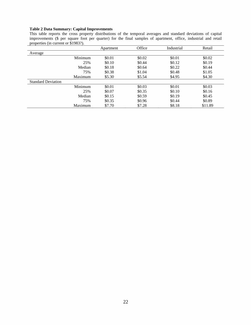
Table 2 summarizes the temporal average and standard deviation of quarterly capital
improvement ($ per square foot) for the four property types (1983 dollars). The reported
statistics are the minimum, 25%, median, 75%, and the maximum of the cross property
distributions of the temporal averages and standard deviations. The median temporal average
capital improvement per square foot per quarter is about 18 cents for apartments, 64 cents for
offices, 22 cents for industrial, and 44 cents for retails. The median of the temporal standard
deviation is 15 cents for apartment, 59 cents for office, 19 cents for industrial, and 45 cents for
retail properties. Figure 2 plots the histograms of the log capital improvement (log $ per square
foot per quarter) of the final samples in the four property types respectively, which appears to
indicate that the log normal distribution is appropriate in describing the capital improvement.
V. Empirical results
We first estimate the parameters of a fixed effect panel regression for the four property types
respectively, using the cross-sectional measure of the cap rate volatility. Table 3 reports the
estimation results, which provides strong evidence for the non-monotonic effect of interest rate
changes on the capital improvement for apartment, office, and retail properties, but no evidence
of this relationship for industrial properties. Specifically, the coefficient of the interaction term
between the change in the interest rate and the cap rate is statistically significant at the 1% level
for apartments, and at the 5% level for office and retail.
We use simulations to illustrate the magnitude of the non-monotonic effect of interest rate
changes on capital improvements for apartment, office, and retail properties respectively. For
each property type, assuming that the interest rate decreases by 50 basis points, we randomly
draw 10,000 sets of coefficients 1 and 2 from the Normal distribution of the coefficient
16
estimators. For each set of 1 and 2 , we calculate 1 2 ,t t i tInt Int Cap with tInt being
fixed at 0.05 (50 basis points), and ,i tCap ranging between 4% and 10%. Since the dependent
variable is the log of the capital improvement, the exponential of 1 2 ,t t i tInt Int Cap has a
straightforward interpretation – it equals the percentage change in the capital improvement as the
result of the change in the interest rate, and this percentage change is a function of the cap rate.
Using the 10,000 sets of drawn coefficients, we are able to construct the percentiles of the
percentage changes in the capital improvement for different cap rates.
Figure 3 plots the 5%, the median, and the 95% of the distribution of the percentage changes in
the capital improvement against the cap rate for apartments. It is clear that the effect decreases
with the cap rate. Specifically, when the cap rate is low, say 4%, the median effect is about 18%,
which means that the capital improvement increases by about 18% if the interest rate decreases
by 50 basis points. However, when the cap rate is high, say 10%, the median effect is only 4%.
Figures 4 and 5 plot the same percentiles for office and industrial properties, and both illustrate
similar patterns: that the effect of a decrease in the interest rate is a decreasing function of the
cap rate. It is worth noting that the non-monotonic effect seems stronger for retail properties
than for apartments and office: the effect decreases from 31%, when the cap rate is 4%, to 0,
when the cap rate is about 7.5%.
Table 3 also indicates that variables other than interest rate changes also influence capital
improvements. First, a change in the cap rate has a negative influence on capital improvements,
and the effect is statistically significant at the 1% level for apartment and office properties, but
insignificant for industrial and retail properties. The negative effect of the cap rate is consistent
with the notion that the lower is the cap rate, the higher is the expected growth rate of future NOI
or the lower is the cost of capital, both of which indicates higher NPV of new investment and
thus more expenditures on capital improvements. Second, the physical condition of the property,
which is measured with the quarterly average of capital improvement from acquisition to the
previous quarter, has a negative effect on the capital improvement. This result is sensible –
holding constant the initial physical condition of a property at acquisition, the more capital
improvement since acquisition, the better is the current physical condition of the property, and
the less is the need for capital improvement. Third, the holding period and its squared value
17
have significant effects for apartment, industrial, and retail properties. This is consistent with the
notion that, holding constant the age of the property at acquisition, the need for capital
improvement changes with the holding period as the property ages. Finally, the dummy for the
quarter after acquisition is negative and statistically significant for apartment, office, and
industrial properties, and the dummy for the quarter before the transfer of ownership is
significantly positive for all property types. This seems to indicate that property owners less
likely invest in capital improvement immediately after the acquisition, and more likely invest
immediately before the disposition.
It is worth noting that Table 3 provides little evidence for the effect of the cap rate volatility on
capital improvement. The coefficient for the cap rate volatility is insignificant for apartment,
office, and industrial properties, and is significantly negative for retail properties. In addition,
Table 3 provides no evidence for the real option effect, which is captured by the interaction term
between the cap rate and the cap rate volatility. Real option theory predicts that the effect of the
expected income growth rate is dampened by the volatility of the expected growth rate, and thus
the coefficient of the interaction term is expected to be significant. However, it is not different
from 0 for all four property types.
A possible reason why Table 3 provides no evidence for the effect of the cap rate volatility and
the real option effect is that perhaps the cap rate volatility is not measured accurately. To
investigate this possibility, we reproduce the regressions in Table 3 but use a temporal measure
of cap rate volatility. These results are reported in Table 4. It is worth noting that Table 4 still
provides strong evidence for the non-monotonic effect of interest rate changes. Specifically, the
coefficient of the interaction term between the interest rate change and the cap rate is statistically
significant for apartment, office, and retail properties. Further, other significant variables shown
in Table 3, including the cap rate, the physical condition, the holding period, and the dummies
for quarters after acquisition and before ownership transfer, remain statistically significant.
Table 4 still provides little evidence for the effect of the cap rate volatility – the coefficient is
only significant for apartments, and the real option effect – the interaction term between the cap
rate and the cap rate volatility--is only significant for retail properties.
18
We conduct a series of robustness checks by changing the data cleaning procedure and then re-
estimate (8). First, when excluding possible opportunistic acquisitions, we exclude properties
that have holding periods shorter than 6 quarters instead of 4 quarters. Second, when excluding
capital improvement outliers, we try a variety of different thresholds, including the top 1%, 1.5%,
and 3%, instead of the top 2.5%. Third, instead of filtering out all properties with at least one 0
capital improvement, we keep them in the sample. The non-monotonic effect of interest rate
changes survives all these robustness checks2, so the strong evidence of the effect do not seem to
be driven by the specific data cleaning procedure we use.
VII. Conclusion
This paper empirically analyzes a non-monotonic effect of interest rate changes on irreversible
investment, which is that the investment response to interest rate changes depends on the
difference between the interest rate and the expected future income growth rate. Using the
complete history of quarterly capital improvement for 1,416 commercial properties over the
1978 to 2009 period, we find strong evidence of the non-monotonic effects for apartment, office,
and retail properties, but no evidence for industrial properties. For the first three property types,
a decrease in the Treasury yield dramatically increases capital improvements when property
values are high (or when cap rates are low), but has a weak or negative influence when properties
have low valuation (high cap rates). This result has a clear and important policy implication. If
a decrease in the interest rate does not necessarily stimulate investment, then monetary
authorities should take extreme care when they try to use interest rate changes to promote
investment.
2 These results are available from the authors.
19
References
Bloom, Nick, Stephen Bond, and John Van Reenen, 2007, Uncertainty and investment dynamics, Review of Economic Studies 74, 391-415.
Bulan, Laarni, Christopher Mayer, and C. Tsuriel Somerville, 2009, Irreversible investment, real options, and competition: Evidence from real estate development, Journal of Urban Economics 65, 237-251.
Capozza, Dennis, and Yuming Li, 1994, The intensity and timing of investment: The case of land, American Economic Review 84, 889-904.
Capozza, Dennis R., and Yuming Li, 2001, Residential investment and interest rates: An empirical test of land development as a real option, Real Estate Economics 29, 503-519.
Capozza, Dennis R., and Yuming Li, 2002, Optimal land development decisions, Journal of Urban Economics 51, 123–142.
Chetty, Raj, 2007, Interest rates, irreversibility, and backward-bending investment, Review of Economic Studies 74, 67-91.
Dixit, Avinash K., and Robert S. Pindyck, 1994, Investment under uncertainty, Princeton University Press, Princeton, N.J.
Fu, Yuming, and Maarten Jennen, 2009, Office construction in singapore and hong kong: Testing real option implications, Journal of Real Estate Finance and Economics 38, 39-58.
Gordon, Myron J., 1962, The investment, financing, and valuation of the corporation, Homewood, Illinois: Richard D. Irwin, Inc.
Grenadier, Steven R., 2002, Option exercise games: An application to equilibrium investment strategies of firms, Review of Financial Studies 15, 691-721.
Guiso, Luigi, and Giuseppe Parigi, 1999, Investment and demand uncertainty, Quarterly Journal of Economics 114, 185-227.
Holland, A. Steven, Steven H. Ott, and Timothy J. Riddiough, 2000, The role of uncertainty in investment: An examination of competing investment models using commercial real estate data, Real Estate Economics 28, 33-84.
Jorgenson, Dale W., 1963, Capital theory and investment behavior, American Economic Review Papers and Proceedings 53, 247–259.
Leahy, John V, and Toni Whited, 1996, The effect of uncertainty on investment: Some stylized facts, Journal of Money, Credit and Banking 28, 64-83.
Moel, Alberto, and Peter Tufano, 2002, When are real options exercised? An empirical study of mine closings, Review of Financial Studies 15, 35-64.
Novy-Marx, Robert, 2007, An equilibrium model of investment under uncertainty, Review of Financial Studies 20, 1461-1502.
Peng, Liang, 2010, Risk and returns of commercial real estate: A property level analysis, Available at SSRN: http://ssrn.com/abstract=1658265.
Pindyck, Robert S., 1991, Irreversibility, uncertainty, and investment, Journal of Economic Literature 29, 1110-1148.
Quigg, Laura, 1993, Empirical testing of real option-pricing models, Journal of Finance 48, 621-640.
Schwartz, E.S. and W. Torous, 2007, Commercial office space: Testing the implications of real options models with competitive interactions, Real Estate Economics 35, 1-20.
Schwartz, Eduardo S., and Lenos Trigeorgis, 2001, Real options and investment under uncertainty: Classical readings and recent contributions, The MIT Press. ISBN 10:-0262-19446-5.
20
Sivitanidou, Rena, and Petros Sivitanides, 2000, Does the theory of irreversible investments help explain movements in office-commercial construction?, Real Estate Economics 28, 623-661.
Titman, Sheridan, 1985, Urban land prices under uncertainty, American Economic Review 75, 505-514.
Trigeorgis, Lenos, 1996, Real options: Managerial flexibility and strategy in resource allocation, MIT Press. Cambridge, MA. ISBN 0-262-20102-X.
Wang, Ko, and Yuqing Zhou, 2006, Equilibrium real options exercise strategies with multiple players: The case of real estate markets, Real Estate Economics 34, 1-49.
Williams, Joseph T., 1997, Redevelopment of real assets, Real Estate Economics 25, 387-407.
21
Table 1 Data Summary: Properties This table reports the following summary statistics for the final samples of apartment, office, industrial and retail properties respectively: the number of different CBSAs where properties are located, the number of properties that had been sold and not sold by 2009:3, the minimum, median, and maximum of the holding periods of properties that had been sold and not sold, the minimum, median, and maximum of the real acquisition price ($ millions in 1983 dollars). Apartment Office Industrial Retail CBSAs 36 32 32 25 Properties
Sold by 2009:3 309 192 170 49 Not Yet Sold 367 210 80 39
Total 676 402 250 88 Holding Period for Sold Properties
Min 5 5 5 5 Median 14 12 9 12
Max 70 38 56 25 Holding Period for Properties Not Yet Sold
Min 4 4 4 7 Median 13 12 13 12
Max 57 48 51 29 Acquisition Price ($ millions)
Min 2.09 1.45 0.23 2.84 Median 13.57 22.10 10.22 14.77
Max 234.50 453.49 470.25 261.33
22
Table 2 Data Summary: Capital Improvements This table reports the cross property distributions of the temporal averages and standard deviations of capital improvements ($ per square foot per quarter) for the final samples of apartment, office, industrial and retail properties (in current or $1983?). Apartment Office Industrial Retail Average
Median $0.15 $0.59 $0.19 $0.45 75% $0.35 $0.96 $0.44 $0.89
Maximum $7.70 $7.28 $8.18 $11.89
23
Table 3 Interest Rate Changes and Capital Improvements: Cross Sectional Volatility of Cap Rates This table reports results that analyze the determinants of capital improvements for apartment, office, industrial and retail properties, respectively, using cross-sectional volatility in cap rates to measure volatility.
, 1 2 , 3 4 , 5 , 6 ,
7 , , 8 , 9 , 10 , 11 , 12 , ,2i t i t t i t t t i t i t i t
i t i t i t i t i t i t i t i t
Inv Int Int Cap Int Int Vol Cap Vol
Cap Vol Con Hold Hold Buy Sell u
In the above model, for property i in quarter t , ,i tInv is the log of capital improvement per square foot; tInt and
tInt are the level and the first order difference of the 5-year Treasury bond yield; ,i tCap is the median cap rate of
all properties in the same Central Business Statistical Area (CBSA) as property i ; ,i tVol is the volatility of ,i tCap ,
which is measured with the cross-property standard deviation of property cap rates in the same CBSA in quarter t ;
,i tCon is the physical condition of the property, which is measured with the average capital improvement per
square foot per quarter since acquisition; ,i tHold and ,2i tHold are the holding period and the squared holding
period from acquisition to quarter t ; ,i tBuy is a dummy variable that equals 1 if the property was acquired in
quarter 1t and 0 otherwise; ,i tSell is a dummy variable that equals 1 if the property was sold in quarter 1t
and 0 otherwise; i is a unobserved property dummy that captures property individual heterogeneity.
Heteroskedasticity-robust standard deviations are in parentheses. ***, **, and * indicate a significant level of 1%, 5%, and 10% respectively. Apartment Office Industrial Retail
Table 4 Interest Rate Changes and Capital Improvements: Time Series Volatility of Cap Rates This table reports results that analyze the determinants of capital improvements for apartment, office, industrial and retail properties, respectively, using temporal volatility in cap rates to measure volatility.
, 1 2 , 3 4 , 5 , 6 ,
7 , , 8 , 9 , 10 , 11 , 12 , ,2i t i t t i t t t i t i t i t
i t i t i t i t i t i t i t i t
Inv Int Int Cap Int Int Vol Cap Vol
Cap Vol Con Hold Hold Buy Sell u
In the above model, for property i in quarter t , ,i tInv is the log of capital improvement per square foot; tInt and
tInt are the level and the first order difference of the 5-year Treasury bond yield; ,i tCap is the median cap rate of
all properties in the same Central Business Statistical Area (CBSA) as property i ; ,i tVol is the volatility of ,i tCap ,
which is measured with the standard deviation of the CBSA cap rates in the past three and current quarter; ,i tCon is
the physical condition of the property, which is measured with the average capital improvement per square foot per
quarter since acquisition; ,i tHold and ,2i tHold are the holding period and the squared holding period from
acquisition to quarter t ; ,i tBuy is a dummy variable that equals 1 if the property was acquired in quarter 1t and
0 otherwise; ,i tSell is a dummy variable that equals 1 if the property was sold in quarter 1t and 0 otherwise; i
is a unobserved property dummy that captures property individual heterogeneity. Heteroskedasticity-robust standard deviations are in parentheses. ***, **, and * indicate a significant level of 1%, 5%, and 10% respectively. Apartment Office Industrial Retail
Figure 1. CBSA Cap Rates This figure plots the time series of the mean and two standard deviations above and below the mean of the CBSA median cap rates, for apartment, office, industrial and retail properties respectively.
26
Figure 2. Property CapEx per Square Foot (Log)
27
Figure 3. Interest Rate Changes and Capital Improvement
28
Figure 4. Interest Rate Changes and Capital Improvement
29
Figure 5. Interest Rate Changes and Capital Improvement