INTEREST RATE RISK AND OTHER DETERMINANTS OF POST-WWII U.S. GOVERNMENTDEBT/GDP DYNAMICS
George J. HallThomas J. Sargent
Working Paper 15702http://www.nber.org/papers/w15702
NATIONAL BUREAU OF ECONOMIC RESEARCH1050 Massachusetts Avenue
Cambridge, MA 02138January 2010
We thank Francisco Barillas, Leandro Nascimento, and especially Christian Gromwell for very helpfulresearch assistance. We thank Henning Bohn for helpful comments on an earlier draft. The views expressedherein are those of the authors and do not necessarily reflect the views of the National Bureau of EconomicResearch.
NBER working papers are circulated for discussion and comment purposes. They have not been peer-reviewed or been subject to the review by the NBER Board of Directors that accompanies officialNBER publications.
Interest Rate Risk and Other Determinants of Post-WWII U.S. Government Debt/GDP DynamicsGeorge J. Hall and Thomas J. SargentNBER Working Paper No. 15702January 2010JEL No. E31,E43,H6
ABSTRACT
This paper uses the sequence of government budget constraints to motivate estimates of interest paymentson the U.S. Federal government debt. We explain why our estimates differ conceptually and quantitativelyfrom those reported by the U.S. government. We use our estimates to account for contributions tothe evolution of the debt to GDP ratio made by inflation, growth, and nominal returns paid on debtsof different maturities.
George J. HallDepartment of Economics, Mail Stop 21Brandeis University P.O. Box 549110415 South StreetWaltham, MA 02454-9110and [email protected]
Thomas J. SargentDepartment of EconomicsNew York University19 W. 4th Street, 6th FloorNew York, NY 10012and [email protected]
1 Introduction
This paper shows the contributions that nominal interest payments, the maturity composition ofthe debt, inflation, and growth in real GDP have made to the evolution of the U.S. debt to GDPratio since World War II. Among the questions we answer are these. Did the U.S. inflate awaymuch of the debt by using inflation to pay negative real rates of return? Sometimes, but notusually. Did high net-of-interest deficits send the debt-GDP ratio upward? Substantially duringWorld War II, but not too much after that. How much did growth in GDP help contribute toholding down the debt GDP ratio? A lot. How much did the variation in returns across maturitiesaffect the evolution at the debt to GDP ratio? At times substantially, but on average not muchsince the end of World War II.
Our answers to these questions rely on our own accounting scheme and not the U.S. gov-ernment’s.1 Our accounting emerges from a decomposition of the government’s period-by-periodbudget constraint, to be described in section 2 and justified in detail in appendix A. We useprices of indexed and nominal debt of each maturity to construct one-period holding period yieldson government IOU’s of various maturities. Multiplying the vector of returns by the vector ofquantities outstanding each period then gives us the appropriate concept of interest paymentsthat appears in the government budget constraint.
Unfortunately, the government’s interest payments series fails to measure the concept thatappears in the government budget constraint, the equation that determines the evolution of thedebt to GDP ratio. Appendix B describes how the government’s measure ignores capital gains andlosses on longer term government obligations, an error that is revealed by the absence of holdingperiod yields for longer maturity government obligations in what we think is the government’sformula for interest payments. The government creates its estimate of interest by summing allcoupon payments and adding to that sum a one-period holding period yield times all principalrepayments. The government could drive that measure of interest payments to zero every periodby perpetually rolling over, let us say, zero-coupon 10 year bonds. Such bonds would never paycoupons and never mature: each period they would be repurchased as nine year zero-couponbonds and reissued as fresh 10 year zero-coupon bonds. Though the government accounts wouldput interest payments at zero, the government would still pay interest in the economically relevantsense determined by the government budget constraint.
2 Interest payments in the government budget constraint
Let Yt be real GDP at t and let Bt be the real value of government IOU’s owed the public. Thatleast controversial equation of macroeconomics, the government budget constraint, accounts forhow a nominal interest rate rt−1,t, net inflation πt−1,t, net growth in real GDP gt−1,t, and thenet-of-interest deficit deft combine to determine the evolution of the government debt-GDP ratio:
Bt
Yt= (rt−1,t − πt−1,t − gt−1,t)
Bt−1
Yt−1+
deftYt
+Bt−1
Yt−1. (1)
1Meaning the Treasury and the NIPA.
2
The appropriate concept of a nominal return rt−1,t is one that verifies this equation.2
The nominal yield rt−1,t and the real stock of debt Bt in equation (1) are averages of pertinentobjects across terms to maturity. To bring out some of the consequences of interest rate risk andthe maturity structure of the debt for the evolution of the debt-GDP ratio, we refine equation (1)to recognize that the government pays different nominal one-period holding period returns onthe IOUs of different maturities that compose Bt. Thus, let Bj
t−1 and Bjt−1 be the real values
of nominal and indexed zero coupon bonds of maturity j at t − 1, while Bt−1 =∑n
j=1 Bjt−1 and
Bt−1 =∑n
j=1 Bjt−1 are the total real values of nominal and indexed debt at t− 1; let rj
t−1,t be thenet nominal holding period yield between t− 1 and t on nominal zero-coupon bonds of maturityj; let rj
t−1,t be the net real holding period yield between t − 1 and t on inflation indexed zerocoupon bonds of maturity j.3 Then the government budget constraint expresses the following lawof motion for the debt-GDP ratio:
Bt + Bt
Yt=
n∑
j=1
rjt−1,t
Bjt−1
Yt−1− (πt−1,t + gt−1,t)
Bt−1
Yt−1
+n∑
j=1
rjt−1,t
Bjt−1
Yt−1− gt−1,t
Bt−1
Yt−1
+deftYt
+Bt−1 + Bt−1
Yt−1. (2)
Notice how equation (2) distinguishes contributions to the growth of the debt-GDP ratio thatdepend on debt maturity j from those that don’t. Thus, πt−1,t and gt−1,t don’t depend on j andoperate on the total real value of debt last period; but the holding period yields rj
t−1,t and rjt−1,t
do depend on maturity j and operate on the real values of the maturity j components Bjt−1 and
Bjt−1.
Section 3 describes the behavior of holding period yields across maturities. Section 4 thendisplays the outcome of our accounting exercise by decomposing the evolution of the ratio ofdebt to GDP into components coming from inflation, growth in real GDP, nominal yields, andthe maturity composition of the debt. Appendix A describes the data and the theory of theterm structure of interest rates that we use to construct components of the government budgetconstraint (2). Appendix B compares our estimates of interest payments on the U.S. governmentdebt to quite different estimates reported by the Federal government. Appendix B also reverse
2The nominal value of interest payments from the government to the public isrt−1,tpt−1Bt−1
Yt−1where pt−1 is the
price level at t − 1. Unfortunately, the U.S. government reports something that it calls ‘interest payments’ as acomponent of Federal expenditures, but this is not the same as the term
rt−1,tpt−1Bt−1Yt−1
that belongs in (1). As we
discuss in appendix B, what the government reports presumably was designed to answer some question, but thatquestion is not “what is the appropriate interest payment to record in order to account properly for the motionthrough time of the real government debt owed to the public?”
3In a nonstochastic version of the standard growth model that is widely used in macroeconomics and publicfinance, the net holding period yield on debt is identical for zero-coupon bonds of all maturities (e.g., see Ljungqvistand Sargent, 2011, chapter 11). The presence of risk and possibly incomplete markets changes that.
3
engineers the question that the official government interest series seemingly answers, though weconfess limited success in making sense of that question. To help bring out the quantitativesignificance of the interest rate risk that confronts the government and its creditors, appendixC constructs counterfactual series for the evolution of the debt/GDP series under alternativehypothetical debt-management policies the choice among which would have no impact on theevolution of the debt-GDP ratio in a world without interest rate risk.
3 Risk and return across maturities
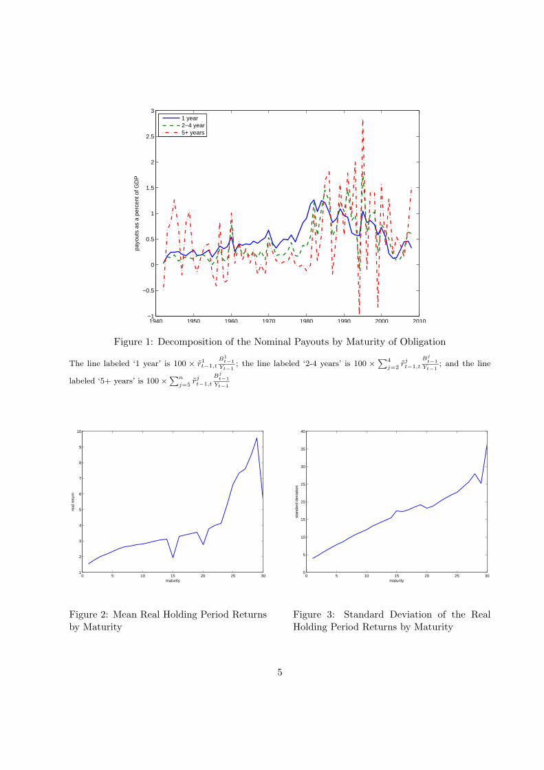
To set the stage for the role that interest rate risks will play in our story, for various maturitiesj measured in years, figure 1 shows contributions to the propulsion of B/Y in formula (1) from
nominal interest payments rjt−1,t
Bjt−1
Yt−1. The figure shows that volatility of nominal interest rate
payments has been larger for longer horizons. For the period 1942-2008, figure 2 plots averageone-year real holding period while figure 3 plots the standard deviation of the one-year real holdingby maturity.4,5 Figure 2 reveals that while longer maturities have generally been associated withhigher and more volatile returns, returns on bonds maturing in 15, 20 and 30 years were onaverage lower than those for adjacent maturities. This outcome reflects investors’ preferences fornewly issued or so-called ‘on the run’ securities.
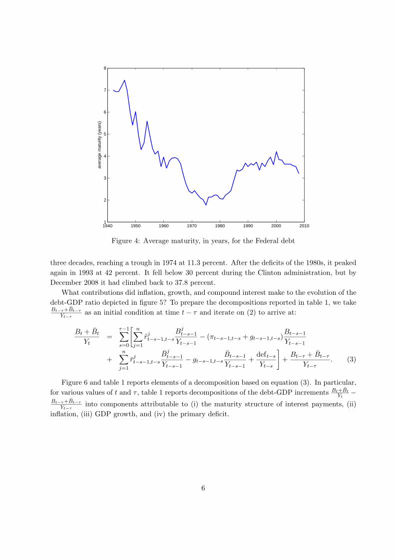
Figure 4 plots the average maturity, in years, of the Treasury debt held by the public. Imme-diately after World War II, the average maturity of the government portfolio was approximately 7years. Over the next three decades, it fell steadily, reaching a trough in the mid-1970s at around2 years. In the 1960s and early 1970s this fall is partly the consequence of federal legislation,repealed in 1975, which prevented the Treasury from issuing long-term instruments paying inter-est above a threshold rate, that market rates exceeded during that period. As we shall see, bycausing the Treasury to shorten the average maturity of its debt during the high inflation yearsof the 1970s, this law prevented the government from fully benefiting from the negative implicitreal interest it managed to pay through inflation. Since the repeal of this restriction, the Treasuryhas lengthened the maturity the average maturity to between 3 and 4 years.
4 Contributions to the evolution of the U.S. debt-GDP ratio
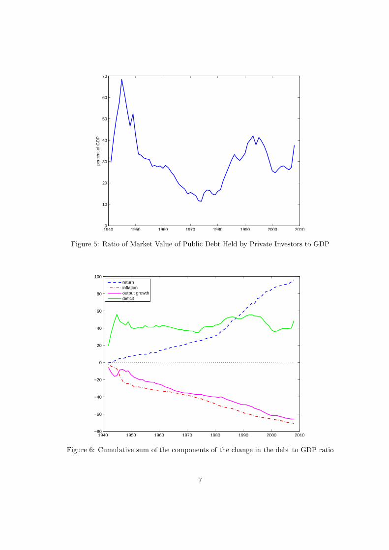
Figure 5 reports the ratio of the market value of U.S. Treasury debt to GDP from 1941 to 2008.6
In 1941, this ratio was 29.6 and in 1945 it stood at 66.2 percent. It fell steadily over the next4A principal aim of stochastic discount factor models like the one proposed by Piazzesi and Schneider (2006) is
to capture how means and standard deviations of one-period holding period yields depend on maturity.5TIPS are not included in the holding period yields in these graphs.6Figure 5 plots the ratio of the end of the calendar year total market value of interest-bearing marketable
Treasury securities held by private investors to GDP. This measure of government debt is narrower than otherFederal debt series sometimes reported. It does not include nonmarketable securities (e.g. savings bonds, specialissues to state and local governments), securities held by other government entities (e.g. the Federal Reserve or theSocial Security Trust Fund), or agency debt (e.g. Tennessee Valley Authority). Further each security is valued atmarket prices rather than par values. See appendix A for a complete description of how this series was constructed.
4
1940 1950 1960 1970 1980 1990 2000 2010−1
−0.5
0
0.5
1
1.5
2
2.5
3
payo
uts
as a
per
cent
of G
DP
1 year2−4 year5+ years
Figure 1: Decomposition of the Nominal Payouts by Maturity of Obligation
The line labeled ‘1 year’ is 100 × r1t−1,t
B1t−1
Yt−1; the line labeled ‘2-4 years’ is 100 × ∑4
j=2rj
t−1,t
Bjt−1
Yt−1; and the line
labeled ‘5+ years’ is 100×∑n
j=5rj
t−1,t
Bjt−1
Yt−1
0 5 10 15 20 25 301
2
3
4
5
6
7
8
9
10
maturity
real
ret
urn
Figure 2: Mean Real Holding Period Returnsby Maturity
0 5 10 15 20 25 300
5
10
15
20
25
30
35
40
maturity
stan
dard
dev
iatio
n
Figure 3: Standard Deviation of the RealHolding Period Returns by Maturity
5
1940 1950 1960 1970 1980 1990 2000 20101
2
3
4
5
6
7
8
aver
age
mat
urity
(ye
ars)
Figure 4: Average maturity, in years, for the Federal debt
three decades, reaching a trough in 1974 at 11.3 percent. After the deficits of the 1980s, it peakedagain in 1993 at 42 percent. It fell below 30 percent during the Clinton administration, but byDecember 2008 it had climbed back to 37.8 percent.
What contributions did inflation, growth, and compound interest make to the evolution of thedebt-GDP ratio depicted in figure 5? To prepare the decompositions reported in table 1, we takeBt−τ+Bt−τ
Yt−τas an initial condition at time t− τ and iterate on (2) to arrive at:
Bt + Bt
Yt=
τ−1∑
s=0
[n∑
j=1
rjt−s−1,t−s
Bjt−s−1
Yt−s−1− (πt−s−1,t−s + gt−s−1,t−s)
Bt−s−1
Yt−s−1
+n∑
j=1
rjt−s−1,t−s
Bjt−s−1
Yt−s−1− gt−s−1,t−s
Bt−s−1
Yt−s−1+
deft−s
Yt−s
]+
Bt−τ + Bt−τ
Yt−τ. (3)
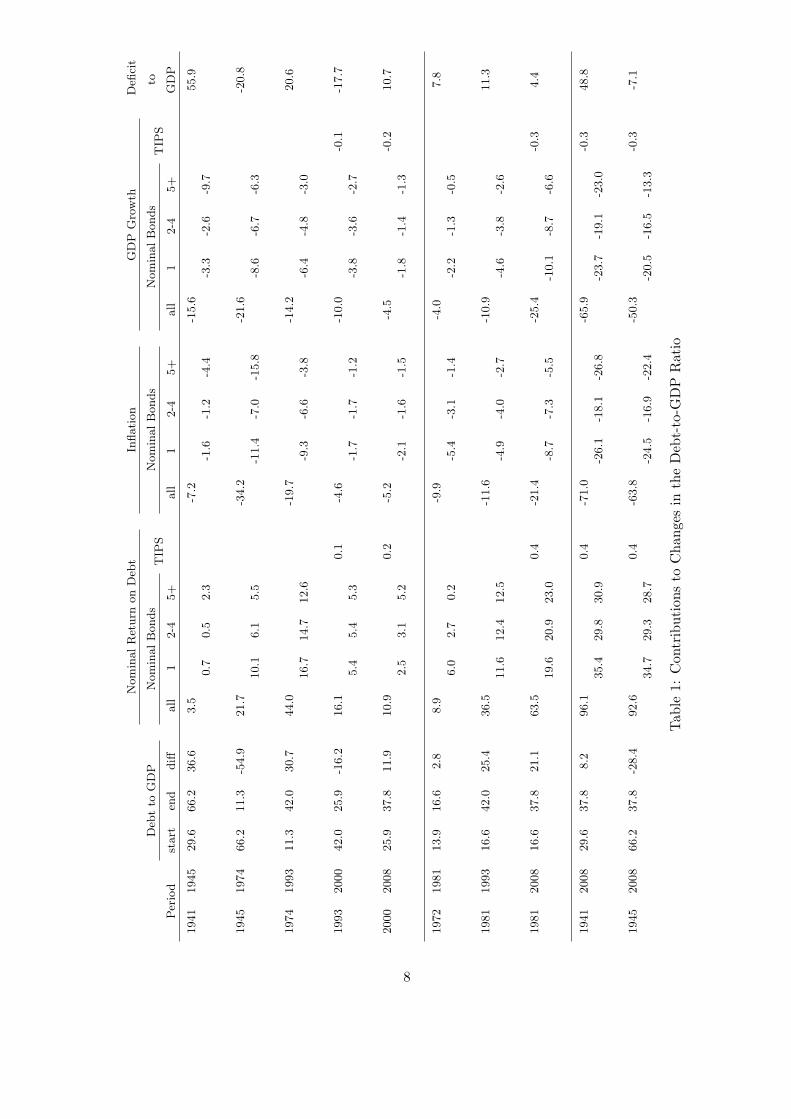
Figure 6 and table 1 reports elements of a decomposition based on equation (3). In particular,for various values of t and τ , table 1 reports decompositions of the debt-GDP increments Bt+Bt
Yt−
Bt−τ+Bt−τ
Yt−τinto components attributable to (i) the maturity structure of interest payments, (ii)
inflation, (iii) GDP growth, and (iv) the primary deficit.
6
1940 1950 1960 1970 1980 1990 2000 20100
10
20
30
40
50
60
70
perc
ent o
f GD
P
Figure 5: Ratio of Market Value of Public Debt Held by Private Investors to GDP
1940 1950 1960 1970 1980 1990 2000 2010−80
−60
−40
−20
0
20
40
60
80
100
returninflationoutput growthdeficit
Figure 6: Cumulative sum of the components of the change in the debt to GDP ratio
7
Nom
inalR
eturn
on
Deb
tIn
flati
on
GD
PG
row
thD
efici
t
Deb
tto
GD
PN
om
inalB
onds
TIP
SN
om
inalB
onds
Nom
inalB
onds
TIP
Sto
Per
iod
start
end
diff
all
12-4
5+
all
12-4
5+
all
12-4
5+
GD
P
1941
1945
29.6
66.2
36.6
3.5
-7.2
-15.6
55.9
0.7
0.5
2.3
-1.6
-1.2
-4.4
-3.3
-2.6
-9.7
1945
1974
66.2
11.3
-54.9
21.7
-34.2
-21.6
-20.8
10.1
6.1
5.5
-11.4
-7.0
-15.8
-8.6
-6.7
-6.3
1974
1993
11.3
42.0
30.7
44.0
-19.7
-14.2
20.6
16.7
14.7
12.6
-9.3
-6.6
-3.8
-6.4
-4.8
-3.0
1993
2000
42.0
25.9
-16.2
16.1
0.1
-4.6
-10.0
-0.1
-17.7
5.4
5.4
5.3
-1.7
-1.7
-1.2
-3.8
-3.6
-2.7
2000
2008
25.9
37.8
11.9
10.9
0.2
-5.2
-4.5
-0.2
10.7
2.5
3.1
5.2
-2.1
-1.6
-1.5
-1.8
-1.4
-1.3
1972
1981
13.9
16.6
2.8
8.9
-9.9
-4.0
7.8
6.0
2.7
0.2
-5.4
-3.1
-1.4
-2.2
-1.3
-0.5
1981
1993
16.6
42.0
25.4
36.5
-11.6
-10.9
11.3
11.6
12.4
12.5
-4.9
-4.0
-2.7
-4.6
-3.8
-2.6
1981
2008
16.6
37.8
21.1
63.5
0.4
-21.4
-25.4
-0.3
4.4
19.6
20.9
23.0
-8.7
-7.3
-5.5
-10.1
-8.7
-6.6
1941
2008
29.6
37.8
8.2
96.1
0.4
-71.0
-65.9
-0.3
48.8
35.4
29.8
30.9
-26.1
-18.1
-26.8
-23.7
-19.1
-23.0
1945
2008
66.2
37.8
-28.4
92.6
0.4
-63.8
-50.3
-0.3
-7.1
34.7
29.3
28.7
-24.5
-16.9
-22.4
-20.5
-16.5
-13.3
Tab
le1:
Con
trib
utio
nsto
Cha
nges
inth
eD
ebt-
to-G
DP
Rat
io
8
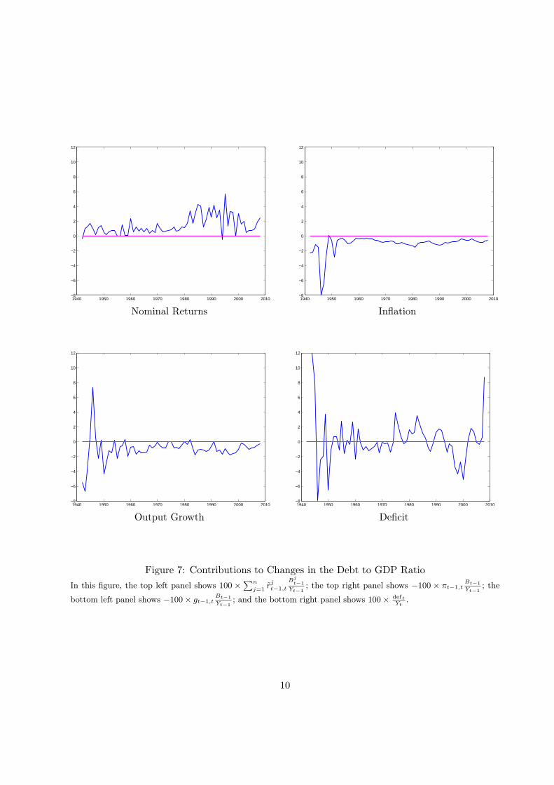
Figure 7 shows the contributions to Bt+BtYt
− Bt−1+Bt−1
Yt−1depicted on the right side of (2). The
top left panel shows 100 × ∑nj=1 rj
t−1,tBj
t−1
Yt−1; the top right panel shows −100 × πt−1,t
Bt−1
Yt−1; the
bottom left panel shows −100 × gt−1,tBt−1
Yt−1; and the bottom right panel shows 100 × deft
Yt. The
nominal returns series plotted in the top left panel is the sum of the three series plotted in figure1.
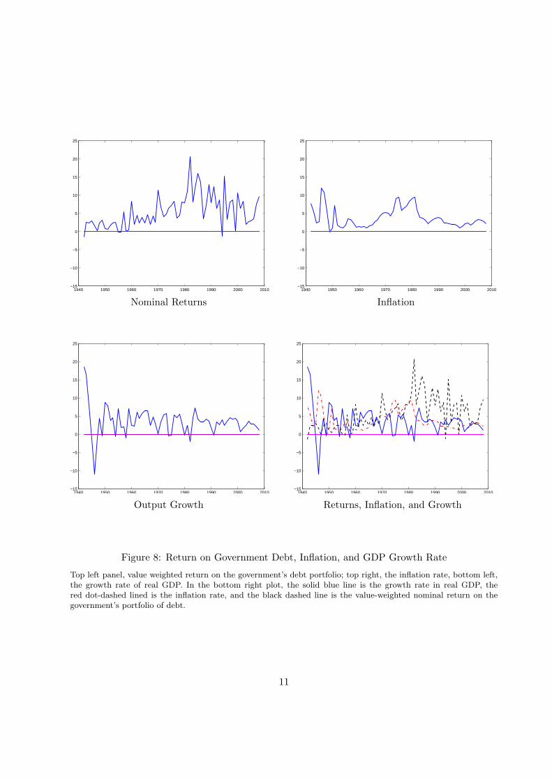
Figure 8 plots the inflation rate, the growth rate of real GDP, and the value weighted return onthe government’s debt portfolio. For the first half of the sample, the growth rate of GDP exceededthe return on the debt, while in the second half of the sample, the return on the government debtexceeded the growth rate.
Table 1 and figures 6, 7, and 8 reveal the following patterns in the way that the U.S. grew,inflated, and paid its way toward higher or lower B/Y ratios:
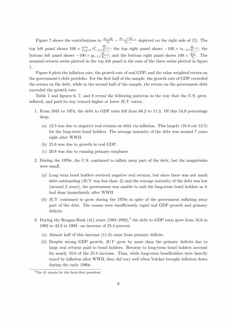
1. From 1945 to 1974, the debt to GDP ratio fell from 66.2 to 11.3. Of this 54.9 percentagedrop,
(a) 12.5 was due to negative real returns on debt via inflation. This largely (10.3 out 12.5)hit the long-term bond holders. The average maturity of the debt was around 7 yearsright after WWII.
(b) 21.6 was due to growth in real GDP.
(c) 20.8 was due to running primary surpluses
2. During the 1970s, the U.S. continued to inflate away part of the debt, but the magnitudeswere small.
(a) Long term bond holders received negative real returns, but since there was not muchdebt outstanding (B/Y was less than .2) and the average maturity of the debt was low(around 2 years), the government was unable to nail the long-term bond holders as ithad done immediately after WWII.
(b) B/Y continued to grow during the 1970s in spite of the government inflating awaypart of the debt. The causes were insufficiently rapid real GDP growth and primarydeficits.
3. During the Reagan-Bush (41) years (1981-1992),7 the debt to GDP ratio grew from 16.6 in1982 to 42.0 in 1993– an increase of 25.4 percent.
(a) Almost half of this increase (11.3) came from primary deficits.
(b) Despite strong GDP growth, B/Y grew by more than the primary deficits due tolarge real returns paid to bond holders. Returns to long-term bond holders accountfor nearly 10.0 of the 25.4 increase. Thus, while long-term bondholders were heavilytaxed by inflation after WWII, they did very well when Volcker brought inflation downduring the early 1980s.
Figure 8: Return on Government Debt, Inflation, and GDP Growth Rate
Top left panel, value weighted return on the government’s debt portfolio; top right, the inflation rate, bottom left,the growth rate of real GDP. In the bottom right plot, the solid blue line is the growth rate in real GDP, thered dot-dashed lined is the inflation rate, and the black dashed line is the value-weighted nominal return on thegovernment’s portfolio of debt.
11
1940 1950 1960 1970 1980 1990 2000 2010−10
−5
0
5
10
15
real
ret
urn
(per
cent
)
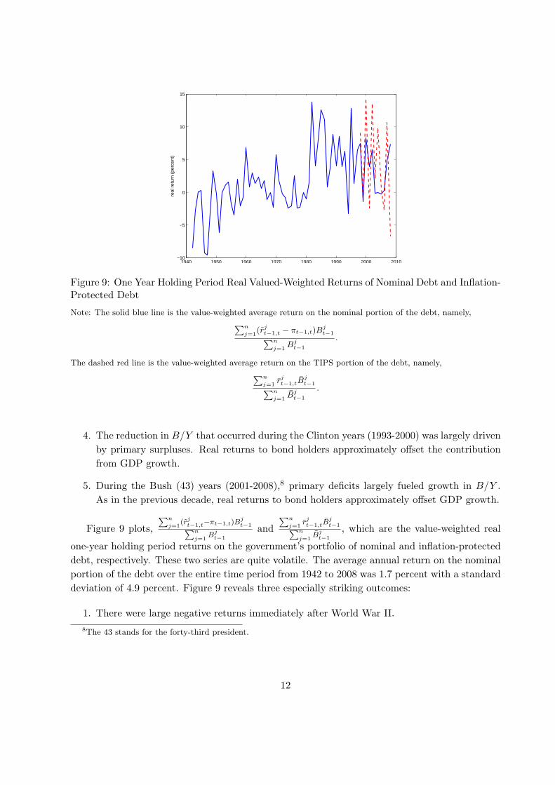
Figure 9: One Year Holding Period Real Valued-Weighted Returns of Nominal Debt and Inflation-Protected Debt
Note: The solid blue line is the value-weighted average return on the nominal portion of the debt, namely,
∑n
j=1(rj
t−1,t − πt−1,t)Bjt−1∑n
j=1Bj
t−1
.
The dashed red line is the value-weighted average return on the TIPS portion of the debt, namely,
∑n
j=1rj
t−1,tBjt−1∑n
j=1Bj
t−1
.
4. The reduction in B/Y that occurred during the Clinton years (1993-2000) was largely drivenby primary surpluses. Real returns to bond holders approximately offset the contributionfrom GDP growth.
5. During the Bush (43) years (2001-2008),8 primary deficits largely fueled growth in B/Y .As in the previous decade, real returns to bond holders approximately offset GDP growth.
Figure 9 plots,∑n
j=1(rj
t−1,t−πt−1,t)Bjt−1∑n
j=1Bj
t−1
and∑n
j=1rjt−1,tB
jt−1∑n
j=1Bj
t−1
, which are the value-weighted real
one-year holding period returns on the government’s portfolio of nominal and inflation-protecteddebt, respectively. These two series are quite volatile. The average annual return on the nominalportion of the debt over the entire time period from 1942 to 2008 was 1.7 percent with a standarddeviation of 4.9 percent. Figure 9 reveals three especially striking outcomes:
1. There were large negative returns immediately after World War II.8The 43 stands for the forty-third president.
12
Variable Mean Std Dev
Nominal Return on Nominal Debt 5.47 4.53Real Return on Nominal Debt 1.69 4.87Inflation 3.77 2.67Nominal GDP growth 7.09 3.77Real GDP growth 3.28 3.43100× Deficit to GDP Ratio 1.07 5.40
Real Return on TIPS (1998-2008) 4.29 7.36Real Return on Nominal Debt (1998-2008) 3.33 3.74
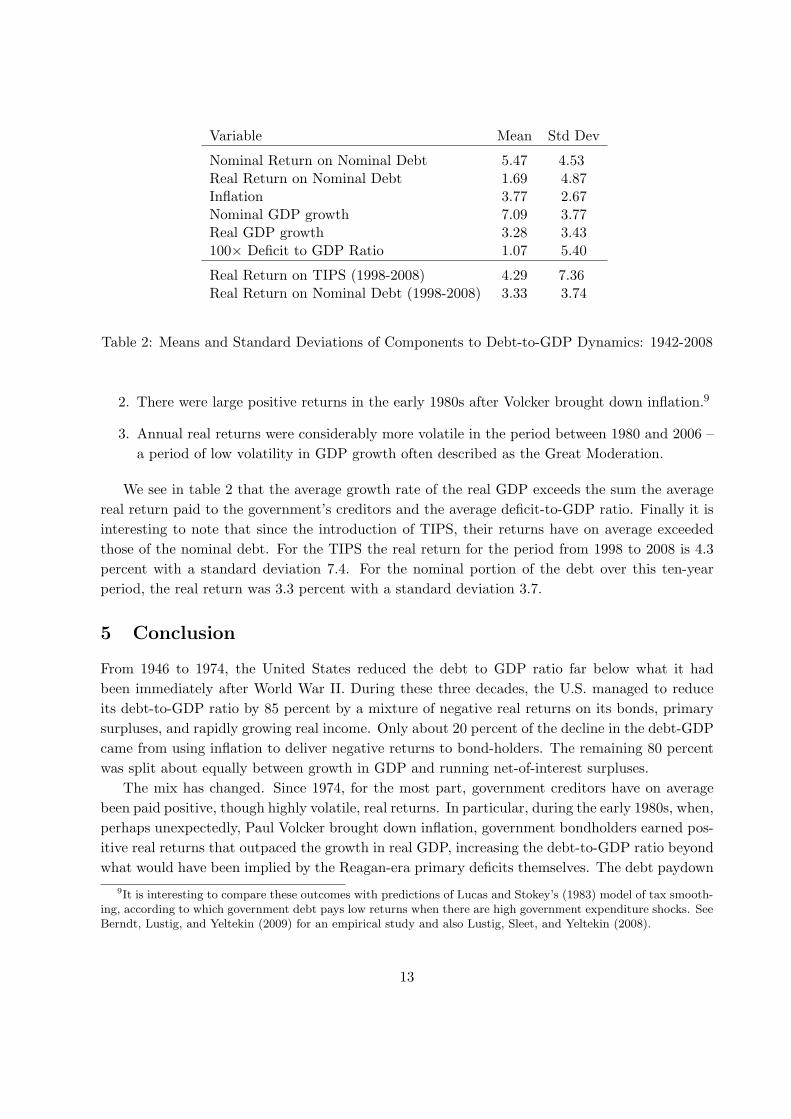
Table 2: Means and Standard Deviations of Components to Debt-to-GDP Dynamics: 1942-2008
2. There were large positive returns in the early 1980s after Volcker brought down inflation.9
3. Annual real returns were considerably more volatile in the period between 1980 and 2006 –a period of low volatility in GDP growth often described as the Great Moderation.
We see in table 2 that the average growth rate of the real GDP exceeds the sum the averagereal return paid to the government’s creditors and the average deficit-to-GDP ratio. Finally it isinteresting to note that since the introduction of TIPS, their returns have on average exceededthose of the nominal debt. For the TIPS the real return for the period from 1998 to 2008 is 4.3percent with a standard deviation 7.4. For the nominal portion of the debt over this ten-yearperiod, the real return was 3.3 percent with a standard deviation 3.7.
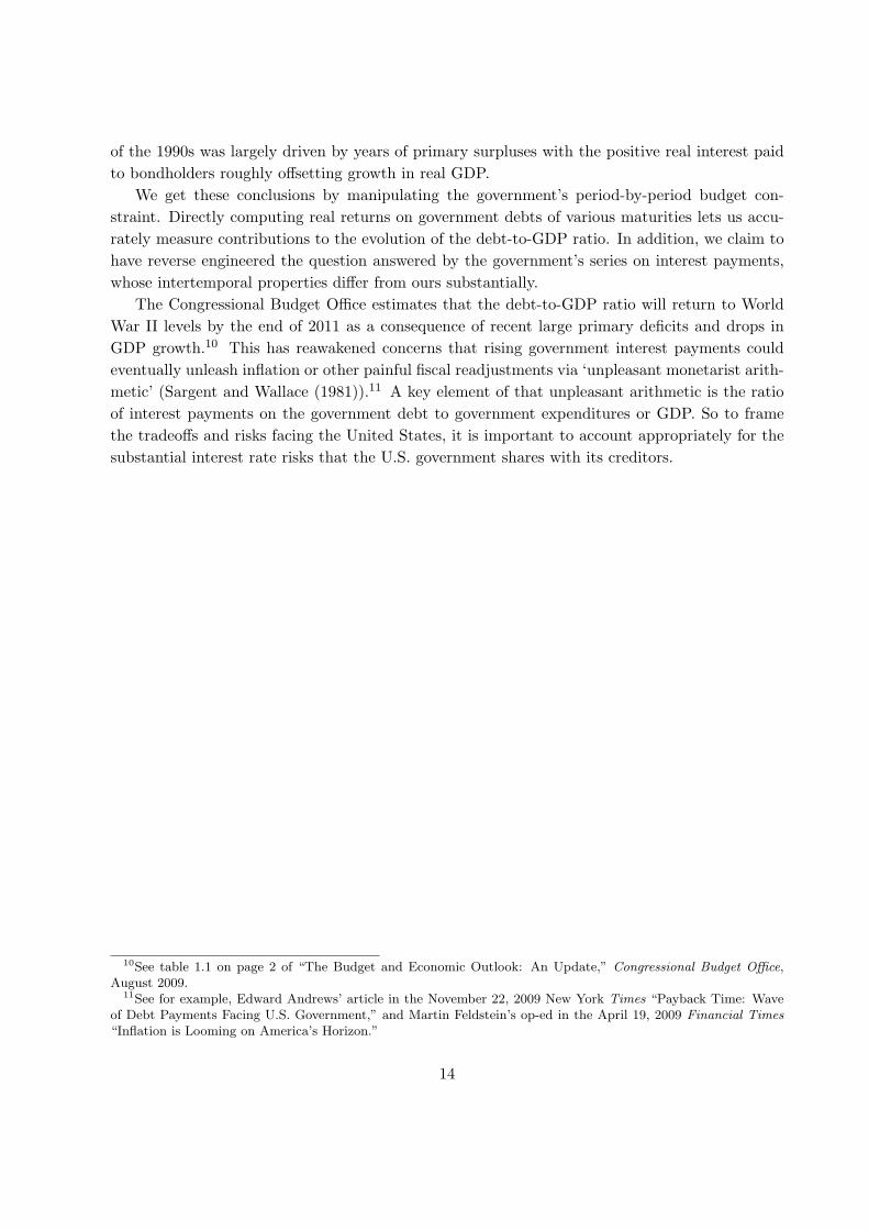
5 Conclusion
From 1946 to 1974, the United States reduced the debt to GDP ratio far below what it hadbeen immediately after World War II. During these three decades, the U.S. managed to reduceits debt-to-GDP ratio by 85 percent by a mixture of negative real returns on its bonds, primarysurpluses, and rapidly growing real income. Only about 20 percent of the decline in the debt-GDPcame from using inflation to deliver negative returns to bond-holders. The remaining 80 percentwas split about equally between growth in GDP and running net-of-interest surpluses.
The mix has changed. Since 1974, for the most part, government creditors have on averagebeen paid positive, though highly volatile, real returns. In particular, during the early 1980s, when,perhaps unexpectedly, Paul Volcker brought down inflation, government bondholders earned pos-itive real returns that outpaced the growth in real GDP, increasing the debt-to-GDP ratio beyondwhat would have been implied by the Reagan-era primary deficits themselves. The debt paydown
9It is interesting to compare these outcomes with predictions of Lucas and Stokey’s (1983) model of tax smooth-ing, according to which government debt pays low returns when there are high government expenditure shocks. SeeBerndt, Lustig, and Yeltekin (2009) for an empirical study and also Lustig, Sleet, and Yeltekin (2008).
13
of the 1990s was largely driven by years of primary surpluses with the positive real interest paidto bondholders roughly offsetting growth in real GDP.
We get these conclusions by manipulating the government’s period-by-period budget con-straint. Directly computing real returns on government debts of various maturities lets us accu-rately measure contributions to the evolution of the debt-to-GDP ratio. In addition, we claim tohave reverse engineered the question answered by the government’s series on interest payments,whose intertemporal properties differ from ours substantially.
The Congressional Budget Office estimates that the debt-to-GDP ratio will return to WorldWar II levels by the end of 2011 as a consequence of recent large primary deficits and drops inGDP growth.10 This has reawakened concerns that rising government interest payments couldeventually unleash inflation or other painful fiscal readjustments via ‘unpleasant monetarist arith-metic’ (Sargent and Wallace (1981)).11 A key element of that unpleasant arithmetic is the ratioof interest payments on the government debt to government expenditures or GDP. So to framethe tradeoffs and risks facing the United States, it is important to account appropriately for thesubstantial interest rate risks that the U.S. government shares with its creditors.
10See table 1.1 on page 2 of “The Budget and Economic Outlook: An Update,” Congressional Budget Office,August 2009.
11See for example, Edward Andrews’ article in the November 22, 2009 New York Times “Payback Time: Waveof Debt Payments Facing U.S. Government,” and Martin Feldstein’s op-ed in the April 19, 2009 Financial Times“Inflation is Looming on America’s Horizon.”
14
A Good accounting
At each date t, we compute the number of dollars the government has promised for each datet + j in the future. We regard a coupon bond consisting of a stream of promised coupons plus anultimate principal payment as a bundle of zero coupon bonds of different maturities. We priceit by unbundling it into a set of component zero-coupon bonds, one for each date at which acoupon on the bond is due, valuing each such component individually, then adding up the valueof the components. In other words, we strip the coupons from the bond and price the bond as aweighted sum of zero coupon bonds of maturities j = 1, 2, ..., n. The market and the governmentalready do this. Prestripped coupon bonds are routinely traded.
We treat nominal bonds and inflation-indexed bonds separately. For nominal bonds, let stt+j
be the number of time t + j dollars that the government has promised to deliver, as of time t.To compute st
t+j from historical data, we add up all of the dollar principal-plus-coupon paymentsthat the government has promised to deliver at date t+ j as of date t. We let st
t+j be the numberof inflation protected t + j dollars, or time t + j goods, that the government has promised todeliver, as of time t.
Since zero-coupon bond prices were not directly observable until prestripped coupon bondswere introduced in 1985, we extract the nominal implicit forward rates from government bondprice data. We then convert these nominal forward rates on government debt into prices of claimson future dollars. Let qt
t+j be the number of time t dollars that it takes to buy a dollar at timet + j:
qtt+j =
1(1 + ρjt)j
≈ exp(−jρjt)
where ρjt is the time t yield to maturity on bonds with j periods to maturity. The yield curveat time t is a graph of yield to maturity ρjt against maturity j. The vector {qt
t+j}nj=1, where n is
the longest maturity outstanding, prices all nominal zero coupon bonds at t. To convert t dollarsto goods we use
vt =1pt
where pt is the price level in base year 2005 dollars, and vt is the value of currency measured ingoods per dollar.
For inflation-protected bonds (TIPS), let stt+j be the number of time t + j goods that the
government promises to deliver at time t. For indexed debt, when we add up the principal andcoupon payments that the government has promised to deliver at date t + j as of date t, we mustadjust for past realizations of inflation in ways consistent with the rules governing TIPS.
To compute a real price of a promise, sold at time t, of goods at time t + j, ρjt, we constructa real yield to maturity as
ρjt = ρjt − πt−1,t
15
where πt−1,t is the inflation rate from t− 1 to t realized at t. We appeal to a random walk modelfor inflation to justify this way of estimating real yields to maturities.12 We then compute qt
t+j ,the number of time t goods that it takes to purchase a time t + j good, by:
qtt+j =
1(1 + ρjt)j
≈ exp(−jρjt).
The total real value of government debt issued in period t equals
vt
n∑
j=1
qtt+js
tt+j +
n∑
j=1
qtt+j s
tt+j .
The first term is the real value of the nominal debt, computed by multiplying the number of timet + j dollars that the government has sold, st
t+j , by their price in terms of time t dollars, qtt+j ,
summing over all outstanding bonds, j = 1, . . . , n, and then converting from dollars to goods bymultiplying by vt. The second term is the value of the inflation-protected debt, computed bymultiplying the number of time t+j goods that the government has promised, st
t+j , by their pricein terms of time t goods, qt
t+j , and then summing over j = 1, . . . , n.
A.1 Constraint on debt management (or open market) policy
At a given date t, the government faces the following constraint on debt management or openmarket operations
vt
n∑
j=1
qtt+j(s
tt+j − st
t+j) +n∑
j=1
qtt+j(s
tt+j − st
t+j) = 0, (4)
where {stt+j}n
j=1 is an alternative portfolio of nominal claims and {stt+j}n
j=1 is an alternative port-folio of real claims. This equation expresses the restriction that the total value of government debtis set by the government’s funding requirements, which are determined by obligations stemmingfrom its borrowing in the past and from its current net-of-interest deficit.
A.2 Government budget constraint, a.k.a. the law of motion for debt
Let deft be the government’s real net-of-interest budget deficit, measured in units of time t goods.The government’s time t budget constraint is:
vt
n∑
j=1
qtt+js
tt+j +
n∑
j=1
qtt+j s
tt+j = vt
n∑
j=1
qtt+j−1s
t−1t+j−1 +
n∑
j=1
qtt+j−1s
t−1t+j−1 + deft, (5)
where it is understood that qtt = 1 and qt
t = vt. The left hand side of equation (5) is the realvalue of the interest bearing debt at the end of period t. The right side of equation (5) is the sumof the real value of the primary deficit deft and the real value of the outstanding debt that thegovernment owes at the beginning of the period, which in turn is simply the real value this period
12See Atkeson and Ohanian (2001) and Stock and Watson (2006) for evidence that a random walk model is agood approximation to inflation in the U.S. since WWII.
16
of outstanding promises to deliver future dollars st−1t−1+j and goods st−1
t−1+j that the governmentissued last period.
To attain the government constraint in the form of equation (2) in the body of our text, wesimply rearrange (5)
∑nj=1 vtq
tt+js
tt+j +
∑nj=1 qt
t+j stt+j
Yt=
n∑
j=1
( vt
vt−1
qtt+j−1
qt−1t+j−1
− 1− gt−1,t
)vt−1qt−1t+j−1s
t−1t+j−1
Yt−1+
+n∑
j=1
( qtt+j−1
qt−1t+j−1
− 1− gt−1,t
) qt−1t+j−1s
t−1t+j−1
Yt−1
+deftYt
+∑n
j=1 vt−1qt−1t+j−1s
t−1t+j−1 +
∑nj=1 qt−1
t+j−1st−1t+j−1
Yt−1. (6)
To see that this equation is equivalent with (2), we use the definitions
vt−1qt−1t+j−1s
t−1t+j−1 = Bj
t−1 (7)
qt−1t+j−1s
t−1t+j−1 = Bj
t−1 (8)
Bt−1 =n∑
j=1
Bjt−1 (9)
Bt−1 =n∑
j=1
Bjt−1 (10)
( vt
vt−1
qtt+j−1
qt−1t+j−1
− 1− gt−1,t
)= rj
t−1,t − πt−1,t − gt−1,t (11)
( qtt+j−1
qt−1t+j−1
− 1− gt−1,t
)= rj
t−1,t − gt−1,t (12)
vt
vt−1= 1 + πt−1,t (13)
Here Bjt−1 and Bj
t−1 defined in (7) and (8) are the real values of nominal and indexed zero-couponbonds (strips) of maturity j at t − 1; Bt−1 and Bt−1 defined in (9) and (10) are the total realvalues of nominal and indexed debt at t − 1; rj
t−1,t defined in (11) is the net nominal holdingperiod yield between t− 1 and t on nominal strips of maturity j; rj
t−1,t defined in (12) is the netreal holding period yield between t− 1 and t on inflation indexed strips of maturity j, and πt−1,t
is the inflation rate between t− 1 and t.
A.3 Data
The price and quantity data for nominal bonds are in the CRSP Monthly Government Bond File.13
The quantity outstanding of the Treasury inflation-protected securities (TIPS) are in December13In the CRSP data set the quantity of publicly held marketable debt only goes back to 1960. We extended this
series using data from the Treasury Bulletin.
17
issues of the U.S Treasury’s Monthly Statement of the Public Debt. For the pre-1970 period, we fita zero-coupon forward curve from the coupon bond price data via Daniel Waggoner’s (1997) cubicspline method. Waggoner fits the zero-coupon one-period forward-rate curve with a cubic splineemploying a set of roughness criteria to reduce oscillations in the approximated curve. For 1970to 2008, we use the nominal and real zero-coupon yield curves computed by Gurkaynak, Sack andWright (2006, 2008). The value of currency vt is the inverse of the fourth quarter observation ofthe GDP price deflator.
As mentioned above, the left side vt∑n
j=1 qtt+js
tt+j +
∑nj=1 qt
t+j stt+j of equation (5) is the real
market value of the interest bearing debt at the end of period t. It excludes nonmarketablesecurities (e.g. savings bonds, special issues to state and local governments), securities held byother government entities (e.g. the Federal Reserve or the Social Security Trust Fund), or agencydebt (e.g. Tennessee Valley Authority). While the Treasury typically reports the par value of thedebt, Seater (1981), Cox and Hirschhorn (1983), Eisner and Peiper (1984), Cox (1985), and Bohn(1992) have calculated series on the market value of the Treasury’s portfolio. Our debt series mostclosely aligns with Seater’s (1981) MVPRIV2 series (see his Table 1) and Cox and Hirschhorn’s(1983) series “Market value of privately held treasury debt” (see their Table 6).
Eisner and Pieper (1984), Eisner (1986), and Bohn (1992) computed similar measures of thegovernment’s interest payments. Rather than computing the terms on the left side of (5) directly,they exploited the inter-temporal budget constraint (1) to compute interest payments rt−1,tBt−1
as the change in the market value of debt minus the primary deficit. An advantage of thatapproach is that there no need to construct the pricing kernels and stripped series; the marketvalue of the debt can be computed directed from the observed prices and quantities outstanding.An advantage of our approach is that since we compute the returns on the debt directly ourmeasure is not sensitive to how the primary deficit is measured. Furthermore, our arithmeticalso allows us (a) to account for the different holding period yields on obligations of differentmaturities and thereby form the decompositions of interest payments in table 1 and figures 1 and6, (b) to execute the counterfactual debt management experiments described in appendix C, and(c) to dissect the difference between our estimates of the interest costs and those reported by theTreasury. We turn to this last task in appendix B.
B Bad accounting: what the government instead reports as in-terest payments
As documented earlier by Hall and Sargent (1997), our estimates of the interest paid on U.S.government debt differ substantially from those reported by the government. In this section,we attempt to track down the sources of differences between our way of accounting for interestand the government’s. Since they give different answers, these two interest payment series mustbe asking different questions. Our series answers the question “what interest payments appearin the law of motion over time of real government indebtedness?”14 What question does the
14The law of motion of real government indebtedness is also known as the government budget constraint.
18
government’s interest payment series answer? And how can we compute it in terms of the objectsq, q, s, s defined in appendix A?
We won’t get much of an answer by reading government reports. Issues of the TreasuryBulletin from 1957 to 1982 contained the following concise description of the government’s methodfor computing its interest expenses:
The computed annual interest charge represents the amount of interest that would bepaid if the interest-bearing issue outstanding at the end of each month or year shouldremain outstanding for a year at the applicable annual rate of interest. The chargeis computed for each issue by applying the appropriate annual interest rate to theamount of the security outstanding on that date.
We interpret these statements to mean that the government computes interest expenses by addingnext year’s coupon payments to the product of the outstanding principal due next year and theone-period holding period yield on one-period pure discount bonds. In this appendix, we shallverify this interpretation by executing this computation with the q, q, s, s series from appendix Aand show that it produces a time series that closely approximates the government’s reported serieson interest payments. Then we’ll try to reverse engineer a question that this series is designedto answer. Finally, we’ll describe in detail how the government’s concept of interest costs failsto match the concept required by the government’s budget constraint (1) or (2) because it treatscoupon payments and capital gains improperly.
To cast the government’s computations in terms of our notation, it is useful to define thedecomposition st−1
t = st−1t (tb) + st−1
t (p) + st−1t (c) where st−1
t (tb) represents the par value of one-period pure discount treasury bills and notes, st−1
t (p) denotes the contribution to st−1t coming
from principal due on longer term bonds that mature at t, and st−1t (c) represents coupon payments
on longer term bonds accruing at time t.Then we believe that the government reports the following object as its nominal interest
payments at time t:
vt
{st−1t (c) +
(1− qt−1
t
)(st−1t − st−1
t (c))}
+{st−1t (c) +
(1− qt−1
t
)(st−1t − st−1
t (c))}
(14)
orvt
{st−1t (c) + r1
t−1,t
(st−1t (tb) + st−1
t (p))}
+{st−1t (c) + r1
t−1,t
(st−1t (tb) + st−1
t (p))}
(15)
The term vtst−1t (c) in the first expression is the real value of the coupon payments on nominal
bonds, while st−1t (c) is the real value of coupon payments on indexed bonds. The term vt
(1 −
qt−1t
)(st−1t − st−1
t (c))
is the real value of all payments except coupons, vt
(st−1t − st−1
t (c))
=
vt
(st−1t (tb) + st−1
t (p)), promised at t − 1 to be paid at t multiplied by the one-period holding
period yield r1t−1,t =
(1 − qt−1
t
)on one-period pure discount bills. The two terms in the second
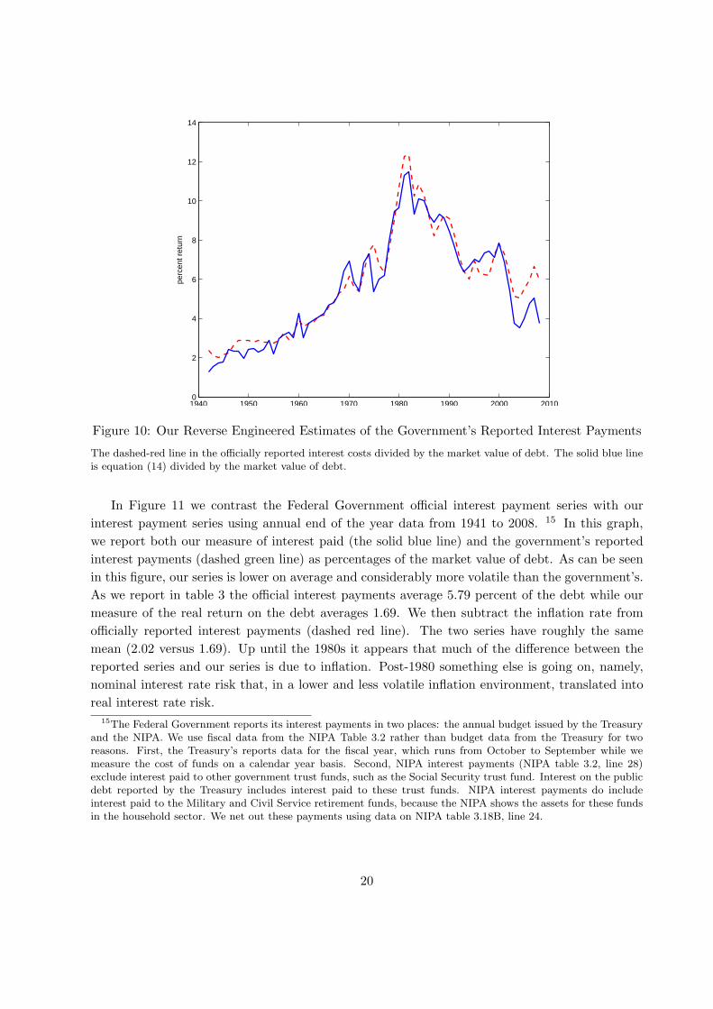
pair of braces are the indexed debt counterparts to the preceding two terms.In figure 10 we plot the government’s official interest payments series and our concept (15).
We divide both series by the market value of debt. The two series track each other quite closely;the correlation coefficient for the two series is 0.97.
19
1940 1950 1960 1970 1980 1990 2000 20100
2
4
6
8
10
12
14
perc
ent r
etur
n
Figure 10: Our Reverse Engineered Estimates of the Government’s Reported Interest Payments
The dashed-red line in the officially reported interest costs divided by the market value of debt. The solid blue lineis equation (14) divided by the market value of debt.
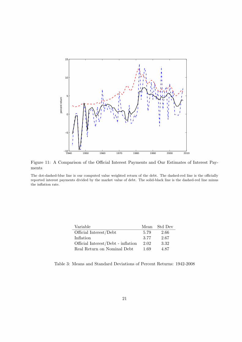
In Figure 11 we contrast the Federal Government official interest payment series with ourinterest payment series using annual end of the year data from 1941 to 2008. 15 In this graph,we report both our measure of interest paid (the solid blue line) and the government’s reportedinterest payments (dashed green line) as percentages of the market value of debt. As can be seenin this figure, our series is lower on average and considerably more volatile than the government’s.As we report in table 3 the official interest payments average 5.79 percent of the debt while ourmeasure of the real return on the debt averages 1.69. We then subtract the inflation rate fromofficially reported interest payments (dashed red line). The two series have roughly the samemean (2.02 versus 1.69). Up until the 1980s it appears that much of the difference between thereported series and our series is due to inflation. Post-1980 something else is going on, namely,nominal interest rate risk that, in a lower and less volatile inflation environment, translated intoreal interest rate risk.
15The Federal Government reports its interest payments in two places: the annual budget issued by the Treasuryand the NIPA. We use fiscal data from the NIPA Table 3.2 rather than budget data from the Treasury for tworeasons. First, the Treasury’s reports data for the fiscal year, which runs from October to September while wemeasure the cost of funds on a calendar year basis. Second, NIPA interest payments (NIPA table 3.2, line 28)exclude interest paid to other government trust funds, such as the Social Security trust fund. Interest on the publicdebt reported by the Treasury includes interest paid to these trust funds. NIPA interest payments do includeinterest paid to the Military and Civil Service retirement funds, because the NIPA shows the assets for these fundsin the household sector. We net out these payments using data on NIPA table 3.18B, line 24.
20
1940 1950 1960 1970 1980 1990 2000 2010−10
−5
0
5
10
15pe
rcen
t ret
urn
Figure 11: A Comparison of the Official Interest Payments and Our Estimates of Interest Pay-ments
The dot-dashed-blue line is our computed value weighted return of the debt. The dashed-red line is the officiallyreported interest payments divided by the market value of debt. The solid-black line is the dashed-red line minusthe inflation rate.
Variable Mean Std DevOfficial Interest/Debt 5.79 2.66Inflation 3.77 2.67Official Interest/Debt - inflation 2.02 3.32Real Return on Nominal Debt 1.69 4.87
Table 3: Means and Standard Deviations of Percent Returns: 1942-2008
21
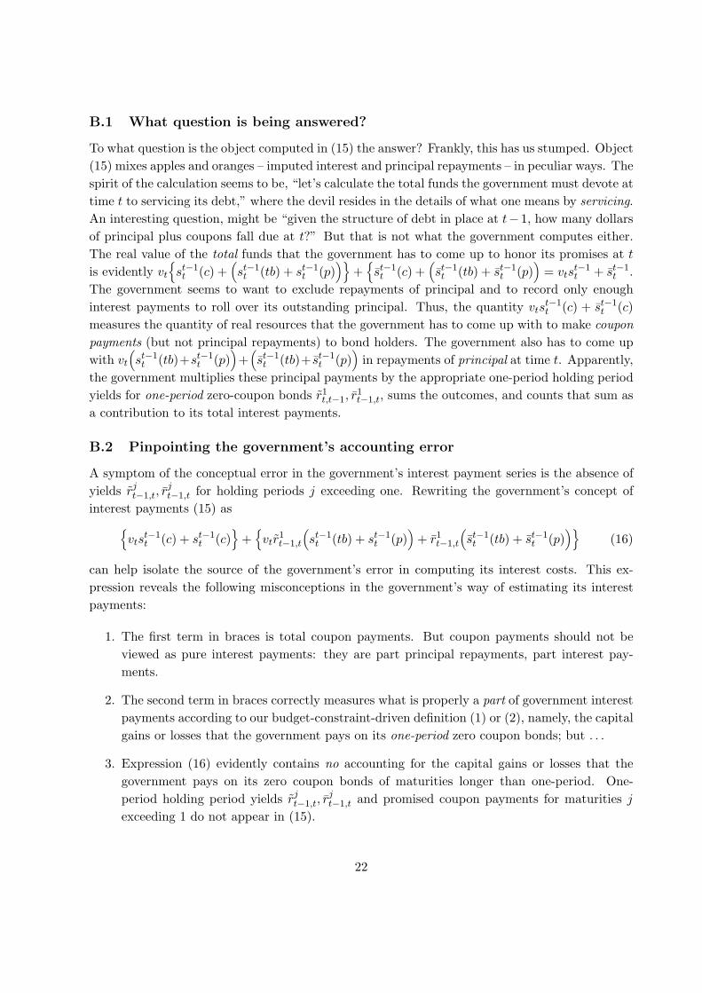
B.1 What question is being answered?
To what question is the object computed in (15) the answer? Frankly, this has us stumped. Object(15) mixes apples and oranges – imputed interest and principal repayments – in peculiar ways. Thespirit of the calculation seems to be, “let’s calculate the total funds the government must devote attime t to servicing its debt,” where the devil resides in the details of what one means by servicing.An interesting question, might be “given the structure of debt in place at t− 1, how many dollarsof principal plus coupons fall due at t?” But that is not what the government computes either.The real value of the total funds that the government has to come up to honor its promises at t
is evidently vt
{st−1t (c) +
(st−1t (tb) + st−1
t (p))}
+{st−1t (c) +
(st−1t (tb) + st−1
t (p))
= vtst−1t + st−1
t .The government seems to want to exclude repayments of principal and to record only enoughinterest payments to roll over its outstanding principal. Thus, the quantity vts
t−1t (c) + st−1
t (c)measures the quantity of real resources that the government has to come up with to make couponpayments (but not principal repayments) to bond holders. The government also has to come upwith vt
(st−1t (tb)+st−1
t (p))+
(st−1t (tb)+ st−1
t (p))
in repayments of principal at time t. Apparently,the government multiplies these principal payments by the appropriate one-period holding periodyields for one-period zero-coupon bonds r1
t,t−1, r1t−1,t, sums the outcomes, and counts that sum as
a contribution to its total interest payments.
B.2 Pinpointing the government’s accounting error
A symptom of the conceptual error in the government’s interest payment series is the absence ofyields rj
t−1,t, rjt−1,t for holding periods j exceeding one. Rewriting the government’s concept of
interest payments (15) as{vts
t−1t (c) + st−1
t (c)}
+{vtr
1t−1,t
(st−1t (tb) + st−1
t (p))
+ r1t−1,t
(st−1t (tb) + st−1
t (p))}
(16)
can help isolate the source of the government’s error in computing its interest costs. This ex-pression reveals the following misconceptions in the government’s way of estimating its interestpayments:
1. The first term in braces is total coupon payments. But coupon payments should not beviewed as pure interest payments: they are part principal repayments, part interest pay-ments.
2. The second term in braces correctly measures what is properly a part of government interestpayments according to our budget-constraint-driven definition (1) or (2), namely, the capitalgains or losses that the government pays on its one-period zero coupon bonds; but . . .
3. Expression (16) evidently contains no accounting for the capital gains or losses that thegovernment pays on its zero coupon bonds of maturities longer than one-period. One-period holding period yields rj
t−1,t, rjt−1,t and promised coupon payments for maturities j
exceeding 1 do not appear in (15).
22
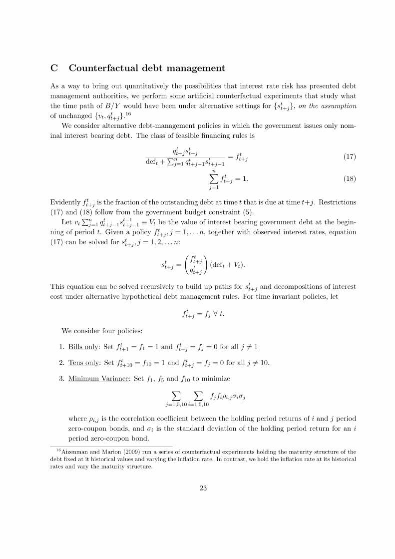
C Counterfactual debt management
As a way to bring out quantitatively the possibilities that interest rate risk has presented debtmanagement authorities, we perform some artificial counterfactual experiments that study whatthe time path of B/Y would have been under alternative settings for {st
t+j}, on the assumptionof unchanged {vt, q
tt+j}.16
We consider alternative debt-management policies in which the government issues only nom-inal interest bearing debt. The class of feasible financing rules is
qtt+js
tt+j
deft +∑n
j=1 qtt+j−1s
tt+j−1
= f tt+j (17)
n∑
j=1
f tt+j = 1. (18)
Evidently f tt+j is the fraction of the outstanding debt at time t that is due at time t+j. Restrictions
(17) and (18) follow from the government budget constraint (5).Let vt
∑nj=1 qt
t+j−1st−1t+j−1 ≡ Vt be the value of interest bearing government debt at the begin-
ning of period t. Given a policy f tt+j , j = 1, . . . n, together with observed interest rates, equation
(17) can be solved for stt+j , j = 1, 2, . . . n:
stt+j =
(f t
t+j
qtt+j
)(deft + Vt).
This equation can be solved recursively to build up paths for stt+j and decompositions of interest
cost under alternative hypothetical debt management rules. For time invariant policies, let
f tt+j = fj ∀ t.
We consider four policies:
1. Bills only: Set f tt+1 = f1 = 1 and f t
t+j = fj = 0 for all j 6= 1
2. Tens only: Set f tt+10 = f10 = 1 and f t
t+j = fj = 0 for all j 6= 10.
3. Minimum Variance: Set f1, f5 and f10 to minimize∑
j=1,5,10
∑
i=1,5,10
fjfiρi,jσiσj
where ρi,j is the correlation coefficient between the holding period returns of i and j periodzero-coupon bonds, and σi is the standard deviation of the holding period return for an i
period zero-coupon bond.16Aizenman and Marion (2009) run a series of counterfactual experiments holding the maturity structure of the
debt fixed at it historical values and varying the inflation rate. In contrast, we hold the inflation rate at its historicalrates and vary the maturity structure.
23
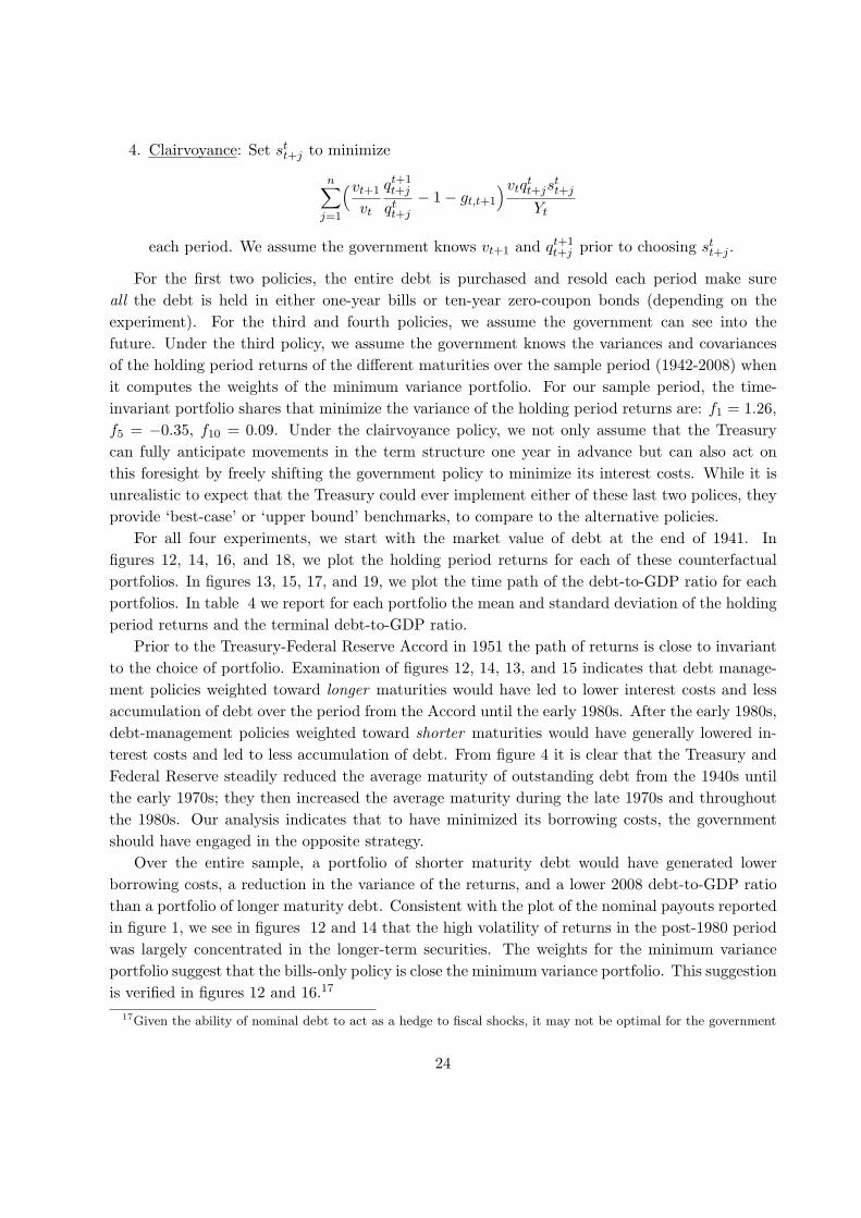
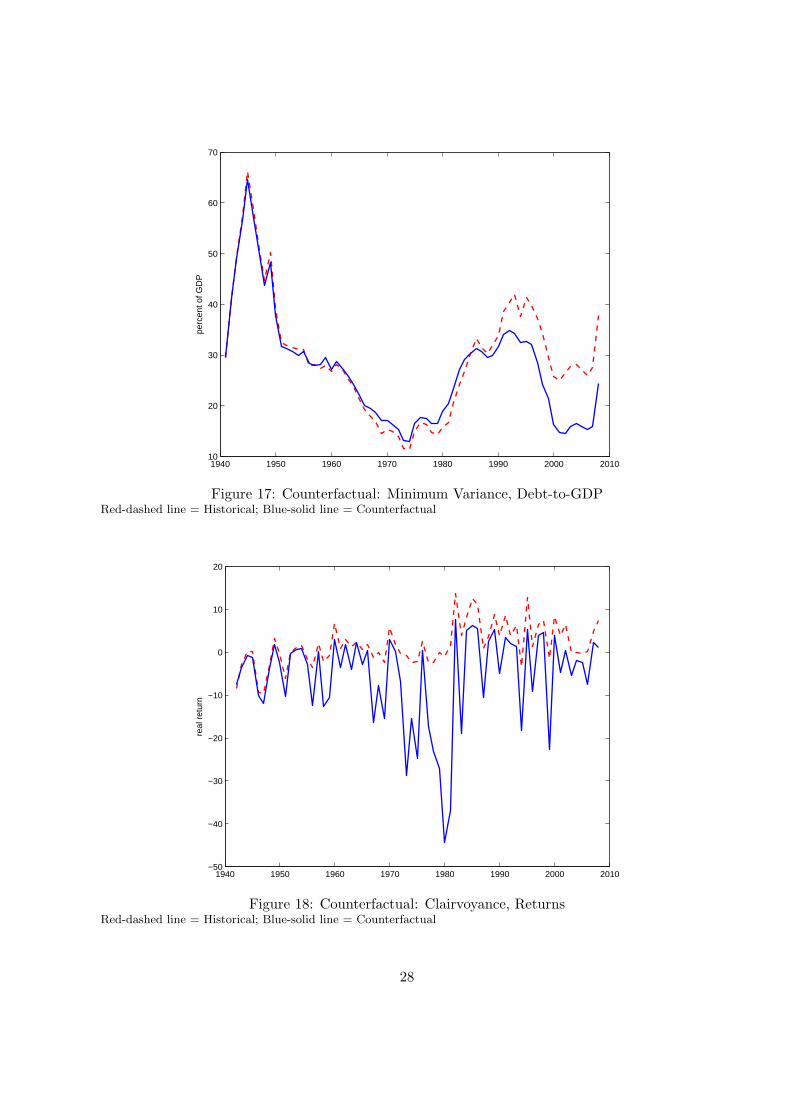
4. Clairvoyance: Set stt+j to minimize
n∑
j=1
(vt+1
vt
qt+1t+j
qtt+j
− 1− gt,t+1
)vtqtt+js
tt+j
Yt
each period. We assume the government knows vt+1 and qt+1t+j prior to choosing st
t+j .
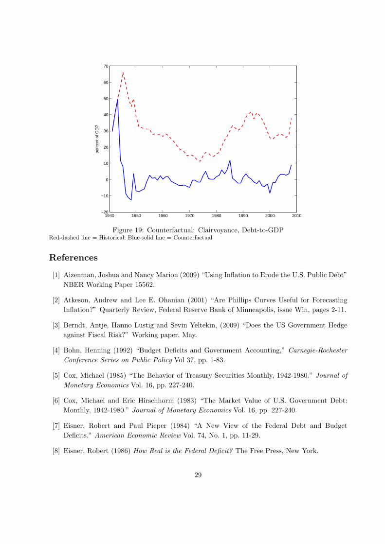
For the first two policies, the entire debt is purchased and resold each period make sureall the debt is held in either one-year bills or ten-year zero-coupon bonds (depending on theexperiment). For the third and fourth policies, we assume the government can see into thefuture. Under the third policy, we assume the government knows the variances and covariancesof the holding period returns of the different maturities over the sample period (1942-2008) whenit computes the weights of the minimum variance portfolio. For our sample period, the time-invariant portfolio shares that minimize the variance of the holding period returns are: f1 = 1.26,f5 = −0.35, f10 = 0.09. Under the clairvoyance policy, we not only assume that the Treasurycan fully anticipate movements in the term structure one year in advance but can also act onthis foresight by freely shifting the government policy to minimize its interest costs. While it isunrealistic to expect that the Treasury could ever implement either of these last two polices, theyprovide ‘best-case’ or ‘upper bound’ benchmarks, to compare to the alternative policies.
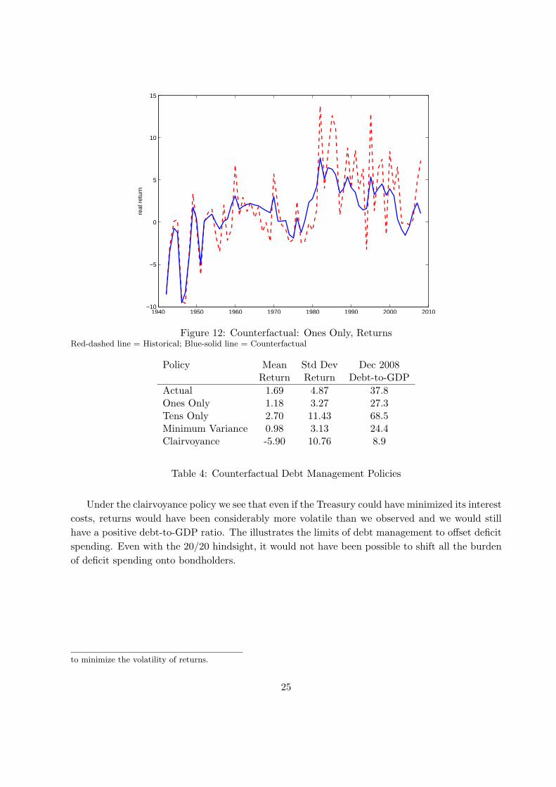
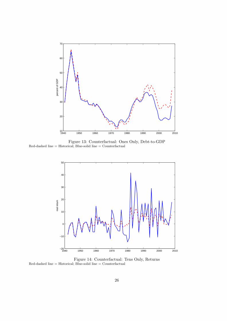
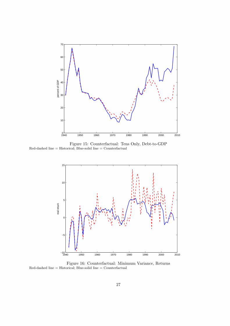
For all four experiments, we start with the market value of debt at the end of 1941. Infigures 12, 14, 16, and 18, we plot the holding period returns for each of these counterfactualportfolios. In figures 13, 15, 17, and 19, we plot the time path of the debt-to-GDP ratio for eachportfolios. In table 4 we report for each portfolio the mean and standard deviation of the holdingperiod returns and the terminal debt-to-GDP ratio.
Prior to the Treasury-Federal Reserve Accord in 1951 the path of returns is close to invariantto the choice of portfolio. Examination of figures 12, 14, 13, and 15 indicates that debt manage-ment policies weighted toward longer maturities would have led to lower interest costs and lessaccumulation of debt over the period from the Accord until the early 1980s. After the early 1980s,debt-management policies weighted toward shorter maturities would have generally lowered in-terest costs and led to less accumulation of debt. From figure 4 it is clear that the Treasury andFederal Reserve steadily reduced the average maturity of outstanding debt from the 1940s untilthe early 1970s; they then increased the average maturity during the late 1970s and throughoutthe 1980s. Our analysis indicates that to have minimized its borrowing costs, the governmentshould have engaged in the opposite strategy.
Over the entire sample, a portfolio of shorter maturity debt would have generated lowerborrowing costs, a reduction in the variance of the returns, and a lower 2008 debt-to-GDP ratiothan a portfolio of longer maturity debt. Consistent with the plot of the nominal payouts reportedin figure 1, we see in figures 12 and 14 that the high volatility of returns in the post-1980 periodwas largely concentrated in the longer-term securities. The weights for the minimum varianceportfolio suggest that the bills-only policy is close the minimum variance portfolio. This suggestionis verified in figures 12 and 16.17
17Given the ability of nominal debt to act as a hedge to fiscal shocks, it may not be optimal for the government
24
1940 1950 1960 1970 1980 1990 2000 2010−10
−5
0
5
10
15
real
ret
urn
Figure 12: Counterfactual: Ones Only, ReturnsRed-dashed line = Historical; Blue-solid line = Counterfactual
Policy Mean Std Dev Dec 2008Return Return Debt-to-GDP
Actual 1.69 4.87 37.8Ones Only 1.18 3.27 27.3Tens Only 2.70 11.43 68.5Minimum Variance 0.98 3.13 24.4Clairvoyance -5.90 10.76 8.9
Table 4: Counterfactual Debt Management Policies
Under the clairvoyance policy we see that even if the Treasury could have minimized its interestcosts, returns would have been considerably more volatile than we observed and we would stillhave a positive debt-to-GDP ratio. The illustrates the limits of debt management to offset deficitspending. Even with the 20/20 hindsight, it would not have been possible to shift all the burdenof deficit spending onto bondholders.
to minimize the volatility of returns.
25
1940 1950 1960 1970 1980 1990 2000 201010
20
30
40
50
60
70
perc
ent o
f GD
P
Figure 13: Counterfactual: Ones Only, Debt-to-GDPRed-dashed line = Historical; Blue-solid line = Counterfactual
1940 1950 1960 1970 1980 1990 2000 2010−20
−10
0
10
20
30
40
50
real
ret
urn
Figure 14: Counterfactual: Tens Only, ReturnsRed-dashed line = Historical; Blue-solid line = Counterfactual
26
1940 1950 1960 1970 1980 1990 2000 20100
10
20
30
40
50
60
70
perc
ent o
f GD
P
Figure 15: Counterfactual: Tens Only, Debt-to-GDPRed-dashed line = Historical; Blue-solid line = Counterfactual
1940 1950 1960 1970 1980 1990 2000 2010−10
−5
0
5
10
15
real
ret
urn
Figure 16: Counterfactual: Minimum Variance, ReturnsRed-dashed line = Historical; Blue-solid line = Counterfactual
27
1940 1950 1960 1970 1980 1990 2000 201010
20
30
40
50
60
70
perc
ent o
f GD
P
Figure 17: Counterfactual: Minimum Variance, Debt-to-GDPRed-dashed line = Historical; Blue-solid line = Counterfactual
1940 1950 1960 1970 1980 1990 2000 2010−50
−40
−30
−20
−10
0
10
20
real
ret
urn
Figure 18: Counterfactual: Clairvoyance, ReturnsRed-dashed line = Historical; Blue-solid line = Counterfactual
28
1940 1950 1960 1970 1980 1990 2000 2010−20
−10
0
10
20
30
40
50
60
70
perc
ent o
f GD
P
Figure 19: Counterfactual: Clairvoyance, Debt-to-GDPRed-dashed line = Historical; Blue-solid line = Counterfactual
References
[1] Aizenman, Joshua and Nancy Marion (2009) “Using Inflation to Erode the U.S. Public Debt”NBER Working Paper 15562.
[2] Atkeson, Andrew and Lee E. Ohanian (2001) “Are Phillips Curves Useful for ForecastingInflation?” Quarterly Review, Federal Reserve Bank of Minneapolis, issue Win, pages 2-11.
[3] Berndt, Antje, Hanno Lustig and Sevin Yeltekin, (2009) “Does the US Government Hedgeagainst Fiscal Risk?” Working paper, May.
[4] Bohn, Henning (1992) “Budget Deficits and Government Accounting,” Carnegie-RochesterConference Series on Public Policy Vol 37, pp. 1-83.
[5] Cox, Michael (1985) “The Behavior of Treasury Securities Monthly, 1942-1980.” Journal ofMonetary Economics Vol. 16, pp. 227-240.
[6] Cox, Michael and Eric Hirschhorm (1983) “The Market Value of U.S. Government Debt:Monthly, 1942-1980.” Journal of Monetary Economics Vol. 16, pp. 227-240.
[7] Eisner, Robert and Paul Pieper (1984) “A New View of the Federal Debt and BudgetDeficits.” American Economic Review Vol. 74, No. 1, pp. 11-29.
[8] Eisner, Robert (1986) How Real is the Federal Deficit? The Free Press, New York.
29
[9] Gurkaynak, Refet S., Brian Sack, and Jonathan Wright (2006) “The U.S. Treasury YieldCurve: 1961 to the Present.” Board of Governors of the Federal Reserve System WorkingPaper 2006-28.
[10] Gurkaynak, Refet S., Brian Sack, and Jonathan Wright (2008) “The TIPS Yield Curve andInflation Compensation.” Board of Governors of the Federal Reserve System Working Paper2008-05.
[11] Hall, George J. and Thomas J. Sargent (1997) “Accounting for the Federal Government’sCost of Funds.” Federal Reserve Bank of Chicago Economic Perspectives Vol 21. No. 4. pp18-28.
[12] Ljungqvist, Lars and Thomas J. Sargent (2011) Recursive Macroeconomic Theory, 3rd edi-tion, MIT Press, Cambridge, Ma.
[13] Lucas, Robert Jr. and Nancy L. Stokey (1983) “Optimal Fiscal and Monetary Policy inan Economy Without Capital.” Journal of Monetary Economics, Elsevier, vol. 12(1), pages55-93.
[14] Lustig, Hanno, Christopher Sleet, and Sevin Yeltekin (2008) “Fiscal Hedging with NominalAssets,” Journal of Monetary Economics, Elsevier, vol. 55(4), pages 710-727.
[15] Piazzesi, Monika and Martin Schneider (2006) “Equilibrium Yield Curves,” MacroeconomicAnnual, edited by Daron Acemoglu, Kenneth Rogoff, and Michael Woodford, National Bu-reau of Economic Research, pages 380-442.
[16] Sargent, Thomas J. and Neil Wallace (1981) “Some Unpleasant Monetarist Arithmetic.”Federal Reserve Bank of Minneapolis Quarterly Review, Fall.
[17] Seater, John (1981) “The Market Value of Outstanding Government Debt, 1919-1975.” Jour-nal of Monetary Economics Vol 8, pp. 85-101.
[18] Stock, James and Mark W. Watson (2006) “Why Has U.S. Inflation Become Harder toForecast?” NBER Working Paper 12324, National Bureau of Economic Research, Inc.
[19] Treasury Bulletin, U.S. Department of Treasury, various issues, 1940-2009.
[20] Waggoner, Daniel (1997) “Spline Methods for Extracting Interest Rate Curves from CouponBond Prices.” Working paper 97-10. Atlanta, Ga.: Federal Reserve Bank of Atlanta.