Interest Rates and Credit Spread Dynamicsfaculty.fiu.edu/~dupoyetb/credit_spreads.pdfFALL 2015 THE...

THE JOURNAL OF DERIVATIVES 25FALL 2015

Interest Rates and Credit Spread DynamicsROBERT NEAL, DOUGLAS ROLPH, BRICE DUPOYET, AND XIAOQUAN JIANG

ROBERT NEAL

is an associate professor of finance at Indiana Univer-sity in Indianapolis, [email protected]

DOUGLAS ROLPH

is a senior lecturer at Nan-yang Business School at Nanyang Technological University in [email protected]

BRICE DUPOYET

is an associate professor of finance at the College of Business at Florida Inter-national University in Miami, [email protected]

XIAOQUAN JIANG

is an associate professor of finance and Knight Ridder Research Fellow at the College of Business at Florida International University in Miami, [email protected]

This article revisits the relationship between call-able credit spreads and interest rates. The authors use cointegration to model the time series of corpo-rate and government bond rates and draw infer-ence about how credit spreads evolve after a shock to government rates using a bootstrapped standard error methodology. They find little evidence that unexpected changes to government rates lead to a significant change in future credit spreads. These results hold for both large positive and negative shocks, as well as after conditioning on the pre-vailing interest rate environment.

Credit spreads are negatively cor-related with interest rates through the impact of changes in interest rates on the credit conditions of

corporations. Most theoretical studies con-sider these correlations in the context of risk-neutral valuation models of corporate debt and focus on the effect that interest rates have on the growth in firm value. These models specify how firm value evolves over time and assume that default is triggered when the firm value falls below some default threshold. The default threshold is a function of the amount of debt outstanding.1 Because the (risk-neutral) growth of the firm increases with the instantaneous risk-free rate, the likelihood that the f irm value falls below the default threshold decreases and the credit risk premium declines. This effect induces a

negative correlation between credit spreads and interest rates.

A number of empirical studies pro-vide evidence of a strong negative rela-tionship between changes in credit spreads and interest rates. The negative correlation between interest rates and credit spreads per-sists after controlling for firm- and market-level determinants of default risk (Longstaff and Schwartz [1995], Collin-Dufresne et al. [2001], Avramov et al. [2007], Campbell and Taksler [2003]). Although the general con-sensus in the literature points to a negative link between credit spreads and government rates, the call feature of corporate debt has the potential to induce a source of common variation in credit spreads and interest rates that is unrelated to default risk ( Jacoby et al. [2009]). For callable bonds, higher interest rates imply a lower chance that the issuer will exercise the call option. Thus, bondholders will accept a lower yield for these call provi-sions, which will result in an overall decrease in the bond yield spread. Although the neg-ative relationship between credit spreads and interest rates weakens for non-callable bonds, there remains a statistically significant decrease in credit spreads for several months following a positive shock to short-term gov-ernment rates (Duffee [1998]).

A common approach in the literature is to regress contemporaneous credit spreads or changes in credit spreads on contemporaneous

JOD-NEAL.indd 25JOD-NEAL.indd 25 8/18/15 4:56:09 PM8/18/15 4:56:09 PM

Auth

or D

raft

for R

evie

w O

nly

26 INTEREST RATES AND CREDIT SPREAD DYNAMICS FALL 2015

levels or changes in Treasury rates. Interest rates and credit spreads, however, have a high degree of persis-tence. The error term of the regression is thus autocorre-lated, correlated with the independent variable (interest rates), and contains information about contemporaneous interest rates. The estimates of the regression coefficients can then be inefficient and the significance tests on the estimated coefficients invalid, as shown in Granger and Newbold [1974]. Our approach is to let the data be our guide by explicitly incorporating the inf luence of per-sistence through the modeling of the joint evolution of corporate and government interest rates using a cointe-gration framework.

We revisit the relationship between credit spreads and interest rates using an improved methodology that combines cointegration with bootstrapped standard errors. Two variables are cointegrated when both are driven by the same unit root process. If corporate rates can be modeled as the sum of the nonstationary Treasury rate and a risk premium, it is clear that both the Treasury and the corporate rates share a common process. Because the two rates are driven by the same stochastic trend, they cannot evolve independently, and the levels of the variables will be linked together.2

Using the cointegration estimates, we examine how credit spreads evolve after an unexpected change in government rates by taking advantage of the gener-alized impulse response function (GIRF) methodology (Koop et al. [1996]). This econometric technique uses bootstrapped standard errors to infer how credit spreads evolve after a shock to government rates. In contrast, many previous empirical studies rely on an assumed dis-tribution of the residuals. Thus, our approach provides a more robust testing framework and accounts for possible fat tails of the empirical distribution of residuals.

Additionally, this approach allows the path of credit spreads to depend on recent levels and changes in government rates. Numerous studies document that government rates and credit spreads contain informa-tion about the current and future state of the macro-economy.3 However, most previous studies focus on the unconditional relationship between credit spreads and government rates. Our approach conditions on current interest rates and allows for asymmetric responses to positive and negative interest rate shocks.

We f ind no statistically signif icant change in credit spreads after large shocks to either short-term or

long-term Treasury yields, either contemporaneously or up to three years after a shock. The results hold for shocks to short, intermediate, and long maturity govern-ment rates and credit spreads constructed with inter-mediate and long maturity corporate bond indexes. These findings contrast with earlier empirical studies that found yields and spreads to be negatively correlated. Our results suggest that how interest rates evolve over time matters for our understanding of the relationship between interest rate shocks and credit spreads.

Our results are interesting for several reasons. First, cointegration has implications for models of pricing cor-porate debt and credit derivatives. Cointegration sup-ports the intuition that corporate and Treasury rates are closely linked and cannot evolve in arbitrary ways. This linkage, however, is not captured in the parameterization of reduced-form bond pricing models, structural models, and credit spread option pricing models. The omission is important because Duan and Pliska [2004] showed that, under reasonable conditions, ignoring cointegra-tion will significantly bias the calculated price of spread options. Second, our finding that higher Treasury rates do not have a statistically significant impact on credit spreads has implications for models that analyze credit spread dynamics. For example, the comparative statics of the capital structure models of Leland and Toft [1996] and Collin-Dufresne and Goldstein [2001] and the bond pricing models of Longstaff and Schwartz [1995], Kim et al. [1993], and Merton [1974] all predict that higher rates will lower credit spreads. Our results suggest that there is little empirical support for this relationship.

DATA AND SUMMARY STATISTICS

We obtain monthly corporate bond yields from the Lehman Brothers U.S. Corporate Index and monthly constant-maturity government rates from the Federal Reserve’s H.15 release. The Lehman Brothers U.S. Cor-porate database begins in 1973, and our study thus spans from February 1973 to December 2007. The Lehman Brothers Corporate Indices include all publicly traded U.S. corporate debentures and secured notes that meet prescribed maturity, liquidity, and quality guidelines. Securities with calls, puts, and sinking fund provisions are included. We consider the effects of interest rate shocks on the credit spreads for bond indexes that differ by credit rating (Aaa, Aa, A, and Baa) and maturity


Auth

or D

raft

for R

evie

w O

nly


(below 10 years for intermediate maturity bonds, and above 10 years for long maturity bonds).

Summary Statistics

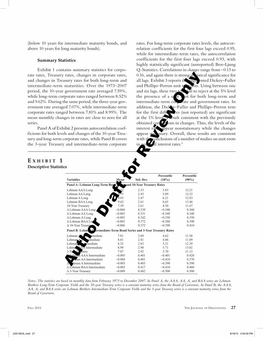
Exhibit 1 contains summary statistics for corpo-rate rates, Treasury rates, changes in corporate rates, and changes in Treasury rates for both long-term and intermediate-term maturities. Over the 1973–2007 period, the 10-year government rate averaged 7.59%, while long-term corporate rates ranged between 8.52% and 9.62%. During the same period, the three-year gov-ernment rate averaged 7.07%, while intermediate-term corporate rates ranged between 7.81% and 8.99%. The mean monthly changes in rates are close to zero for all series.

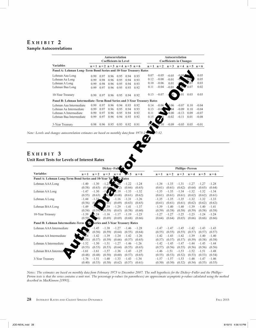
Panel A of Exhibit 2 presents autocorrelation coef-ficients for both levels and changes of the 10-year Trea-sury and long-term corporate rates, while Panel B covers the 3-year Treasury and intermediate-term corporate

rates. For long-term corporate rates levels, the autocor-relation coefficients for the first four lags exceed 0.95, while for intermediate-term rates, the autocorrelation coeff icients for the f irst four lags exceed 0.93, with highly statistically significant (unreported) Box–Ljung Q-Statistics. Correlations in changes range from –0.13 to 0.16, and again there is strong statistical significance for all lags. Exhibit 3 reports the augmented Dickey–Fuller and Phillips–Perron unit root tests. Using between one and six lags, these two tests fail to reject at the 5% level the presence of a unit root for both long-term and intermediate-term corporate and government rates. In addition, the Dickey–Fuller and Phillips–Perron tests for the first differences (not reported) are significant at the 1% level, a result consistent with the previously obtained correlations in changes. Thus, the levels of the interest rates appear nonstationary while the changes appear stationary. Overall, these results are consistent with the conclusions of a number of studies on unit roots in nominal interest rates.4

E X H I B I T 1Descriptive Statistics

Notes: The statistics are based on monthly data from February 1973 to December 2007. In Panel A, the AAA, AA, A, and BAA series are Lehman Brothers Long-Term Corporate Yields and the 10-year Treasury series is a constant maturity series from the Board of Governors. In Panel B, the AAA, AA, A, and BAA series are Lehman Brothers Intermediate-Term Corporate Yields and the 3-year Treasury series is a constant maturity series from the Board of Governors.


Auth

or D

raft

for R

evie

w O

nly


E X H I B I T 3Unit Root Tests for Levels of Interest Rates

Notes: The estimates are based on monthly data from February 1973 to December 2007. The null hypothesis for the Dickey–Fuller and the Phillips–Perron tests is that the series contains a unit root. The percentage p-values (in parentheses) are approximate asymptotic p-values calculated using the method described in MacKinnon [1991].

E X H I B I T 2Sample Autocorrelations

Note: Levels and changes autocorrelation estimates are based on monthly data from 1973:2 to 2007:12.


Auth

or D

raft

for R

evie

w O

nly


COINTEGRATION AND THE UNCONDITIONAL RELATIONSHIP BETWEEN CORPORATE AND TREASURY RATES

The Cointegration Model

In this section, we provide a cointegration frame-work to analyze the relationship between corporate and Treasury bond yields. Cointegration is based on the idea that whereas a set of variables are individually nonsta-tionary, a linear combination of the variables might be stationary due to a long-run statistical relationship linking the cointegrated variables together. Cointe-gration also implies that the short-term movements of the variables will be affected by the lagged deviation from the long-run relationship between the variables, inducing mean reversion around the long-run relation-ship. An alternative view of cointegration is that two variables are cointegrated when both are driven by the same unit root process. If corporate rates can be mod-eled as the sum of the nonstationary Treasury rate and a risk premium, it is clear that both the Treasury and the corporate rates share a common process. Because the two rates are driven by the same stochastic trend, they cannot evolve independently and the levels of the variables will be linked together.5

Assuming stationarity in the changes, the short-term dynamics of two cointegrated variables X

1t and

X2t can be captured in the following error-correction

model:

( )1, 10 1( , 1 2, 1 ,) 11 1,1

, 2,1

1,

X a1 X11

a X

t 10 1 1( ,a t 1) t ii

p

i t,12 2,12 ii

p

t

∑∑

∑

Δ =X1 + γ λ Δa 11+ ∑

Δa 12+ 12∑ + ε

=

−=

(1)

( )2, 20 2( , 1 2, 1 ,) 21 1,1

, 2,1

2,

X a2 X21

a X

t 20 2 1( ,a t 1) t ii

p

i t,22 2,22 ii

p

t

∑∑

∑

Δ =X 2 + γ λ Δa 21+ ∑

Δa 22+ 22∑ + ε

=

−=

(2)

In this model, ε1t and ε

2t represent two i. i. d. error

terms, the cointegration vector is said to be (1,–λ), and the linear combination X

1,t – λX

2,t is stationary. The

economic interpretation of X1,t

– λX2,t

is that it represents the deviation from the long-run relationship between X

1

and X2. This deviation affects the short-term dynamics,

with the error-correction coefficients γ1 and γ

2 describing

how quickly X1 and X

2 respond to the deviation. It is

well known that the presence of cointegration between X

1 and X

2 causes the time series behavior of X to differ

from that of a conventional vector autoregression.6

Equations (1) and (2) can also be written in matrix form as

A X X At A t kA t p t0 1XtX 1 XtΔ =X + Π + ΔA1 Δ +Xt ε1 1 t (3)

where A0 is a (1 × 2) vector of intercepts and A

1 … A

k

are (2 × 2) matrixes of coefficients on lagged ΔX.7 The important characteristic distinguishing cointegration models from VAR models is whether Π = 0. If this restriction holds, then ΔX

t can be represented by a con-

ventional VAR in differences. If the rank of Π exceeds zero, however, the elements of Π are non-zero. We test for cointegration by estimating the rank of Π using Johansen [1988]’s likelihood ratio tests, namely, the maximal eigenvalue test and the trace statistic test.

Vector Error-Correction Model Estimates

The first set of trace statistics in Exhibit 4 exam-ines whether long-term corporate rates (Panel A) and intermediate-term rates (Panel B) share a common unit root with the corresponding government rates. All tests are statistically signif icant at the 5% level. Thus, we reject the null hypothesis that corporate and government yields are not cointegrated in favor of the alternative hypothesis that there is at least one cointegrating vector. The second trace statistics, however, do not support the existence of two cointegrating vectors for either the intermediate-term bond series or the long-term bond series as one cannot reject the null hypothesis of one cointegrating vector or less for any of the series. The results for all series are based on using two lags of the levels of interest rates, with the lag length determined by the Schwartz criterion.

Exhibit 5 reports the estimated cointegrating vec-tors, with λ ranging from 1.1054 to 1.2508 for long maturity bonds, and from 1.0852 to 1.2480 for inter-mediate maturities. The p-values for both panels are less than 1%. The results in Exhibit 5 have two interesting implications. First, because all λ values exceed 1, a 1% increase in Treasury rates ultimately generates increases in corporate rates of more than 1%. Thus, as interest


Auth

or D

raft

for R

evie

w O

nly


rates rise, credit spreads will eventually widen. Second, the lower-quality bonds exhibit a greater long-run sensitivity to interest rate movements than do higher quality bonds. This is inconsistent with a commonly held view that increased credit risk will make corporate bonds less interest rate sensitive.

An alternative way to interpret the cointe-grating relationship is to estimate the error-cor-rection regressions found in Equations (1) and (2). Cointegration implies that the coefficient on the error-correction term will be negative and signifi-cant, with the size of the coefficient measuring the sensitivity of corporate rates to the error-correction term. The negative sign indicates that credit spreads subsequently adjust to restore the long-run equilib-rium when a deviation occurs. Using the estimated cointegrating vectors from Exhibit 5, Exhibit 6 provides estimates of the error-correction model. The error-correction coefficients are significantly negative, ranging from –0.0653 to –0.0511 and from –0.1042 to –0.0619 for long and intermediate maturities respectively.

GIRF AND THE CONDITIONAL RELATIONSHIP BETWEEN CREDIT SPREADS AND TREASURY RATES

The previous section’s results describe the unconditional relationship between credit spreads and Treasury rates. However, conditioning on the current interest rate environment may illuminate how credit spreads evolve following positive and negative shocks to government rates. For example, when the economy is in recession and government rates are relatively low, a positive shock to govern-ment rates may convey different information about future business conditions and credit risk than if the shock occurred during an expansion, when rates are relatively high.

In order to examine the conditional relation-ship between corporate spreads and interest rates, we use the estimates from the second-stage regres-sion in Exhibit 6 to implement the generalized impulse response function (GIRF) methodology of Koop et al. [1996]. When using traditional impulse response functions, the history of the process or the sequence of observations as well as the signs, sizes, and correlations of the shocks occurring between

E X H I B I T 4Cointegration Results

Notes: The estimates are based on monthly data from February 1973 to December 2007. This exhibit uses Johansen’s [1988] maximum likelihood method to estimate the rank of Π for the corporate and government rates in the two-variable regression.

E X H I B I T 5Estimates of Cointegrating Vectors

Notes: The estimates are based on monthly data from February 1973 to December 2007. This exhibit reports estimates of λ in the cointegrating vector (1, –λ) for the corporate and government rates using Johansen’s [1988] maximum likelihood method. The Johansen normalization restrictions are imposed, and we report the coefficient estimates as well as the respective P-values.


Auth

or D

raft

for R

evie

w O

nly


the initial shock and the impulse horizon can produce misleading estimates, as demonstrated by Pesaran and Potter [1997]. The GIRF approach, however, corrects for these issues and allows for asymmetric responses to positive and negative interest rate shocks.

In the GIRF framework, the residuals observed from the VEC model are bootstrapped and the standard errors ref lect the empirical (not assumed) residual distri-bution. Separating the GIRF functions into positive and negative shocks—with possibly different implications regarding the business conditions and their relationship to credit risk—potentially increases the power of the test to reject the null hypothesis of no response. Addi-tionally, traditional impulse response functions’ standard errors rely on a ceteris paribus argument that neglects the effect of the prevailing interest rate environment. In contrast, GIRF functions construct forecasts for each period during the sample using the most recent interest rates and then average over the resulting forecast. Thus, there is more variability in the forecasted path of future credit spreads. The higher variability leads to wider and more realistic standard errors and helps guard against

erroneously concluding shocks to government rates have a statistically significant impact on credit spreads.

GIRF Methodology

The generalized impulse response functions are defined as the difference in month t + i between the con-ditional expectation of the corporate bond spread (corpo-rate yield – Treasury yield) following a shock to Treasury yields exceeding two standard deviations at month t and the conditional expectation across all possible shocks to Treasury yields. Both expectations condition on interest rates at t – 1. The response function describes what might happen to credit spreads in the months following a shock to government rates after controlling for the inf luence of lagged government and corporate rates.

The GIRF equations can be written as follows:

( , ) , 2 )

( ) when 0

1, 1,

1 ,) when

GIRF , )

E(

g t, t1 n t| g ,

t n t g1) when t

ε Ω,,g = Ω( |E | σ

− Ω( |E( t

+) t) (1 E) (E(E − ε21, t, σ

−|n tΩ|

(5)

E X H I B I T 6Estimates of the Error-Correction Model

Notes: This exhibit reports estimates from Equation (1) along with standard errors in parentheses for the bivariate error-correction system of Equations (1) and (2) in the one-lag difference case. The error-correction terms are estimated using Johansen’s [1988] maximum likelihood method. X1 represents the corporate rate, and X2 represents the government rate.


Auth

or D

raft

for R

evie

w O

nly


and as

( , ) , 2 )

( ) when 0

1, 1,

1 ,) when

GIRF ),

E(

g t, t1 n t| g ,

t n t g1) when t

,ε Ω,g = Ω( |E | σ

− Ω( |E( t

+) t) (1 E) (E(E − ε21, t, σ

−|n tΩ|

(6)

where yt+n

is the corporate credit spread at time t + n, Ωt-1

is the time t – 1 information set used to produce forecasts of y

t+n, ε

g,t > 2σε represents a positive shock exceeding

two standard errors, and |εg,t | > 2σε represents a nega-

tive shock exceeding two standard errors.To explain the GIRF procedure, we use a model

which includes one corporate bond rate and one govern-ment bond rate, where

corporate rate at

government rate at,

= 1

1

2

XX

X

t

tt

t

t

=⎡

⎣⎢⎡⎡

⎢⎣⎣⎢⎢

⎤

⎦⎥⎤⎤

⎥⎦⎦⎥⎥ =

⎡

⎣⎢⎡⎡

⎢⎣⎣⎢⎢

⎤

⎦⎥⎤⎤

⎥⎦⎦⎥⎥

Λ −λ⎡⎣⎡⎡ ⎤⎦⎤⎤ (7)

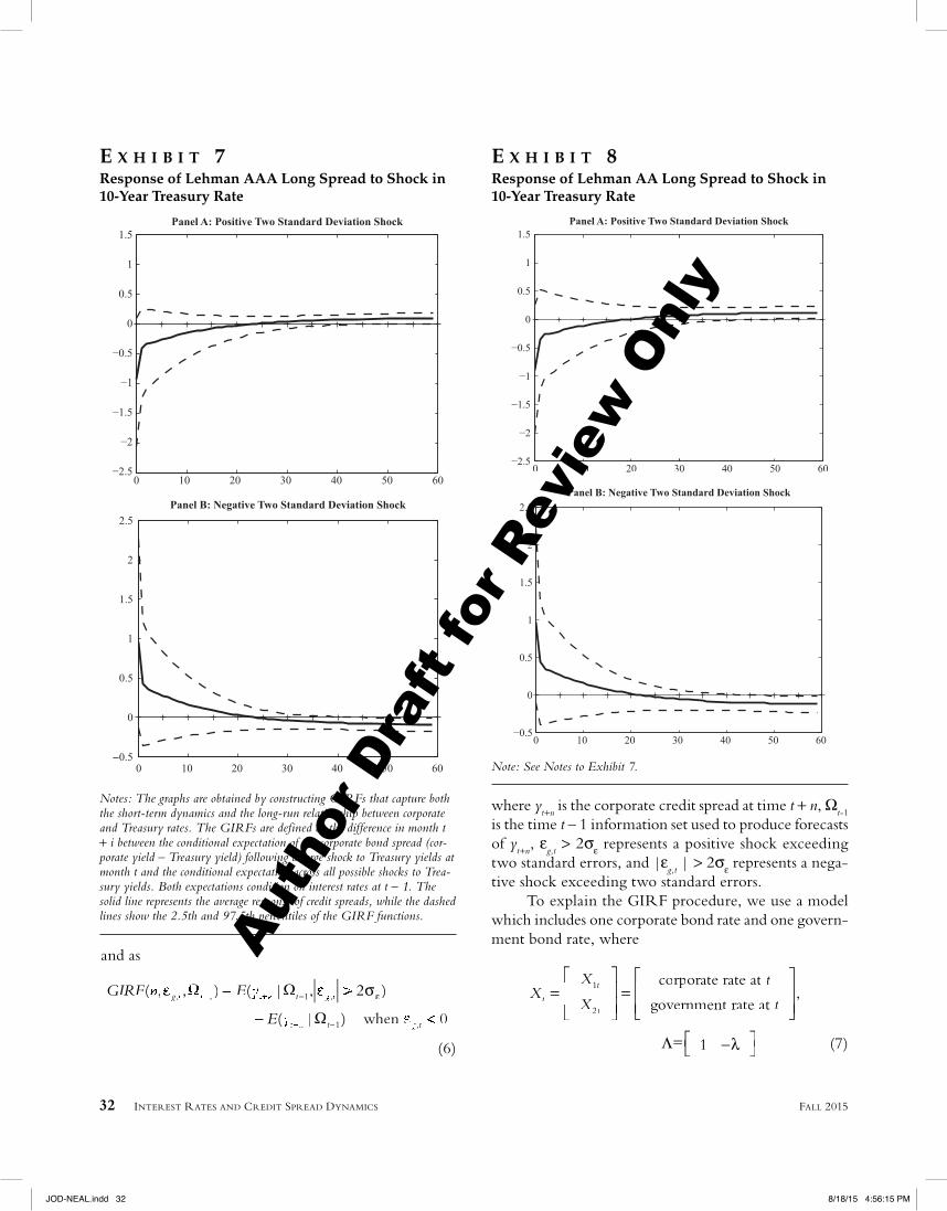
E X H I B I T 8Response of Lehman AA Long Spread to Shock in 10-Year Treasury Rate

Note: See Notes to Exhibit 7.

E X H I B I T 7Response of Lehman AAA Long Spread to Shock in 10-Year Treasury Rate

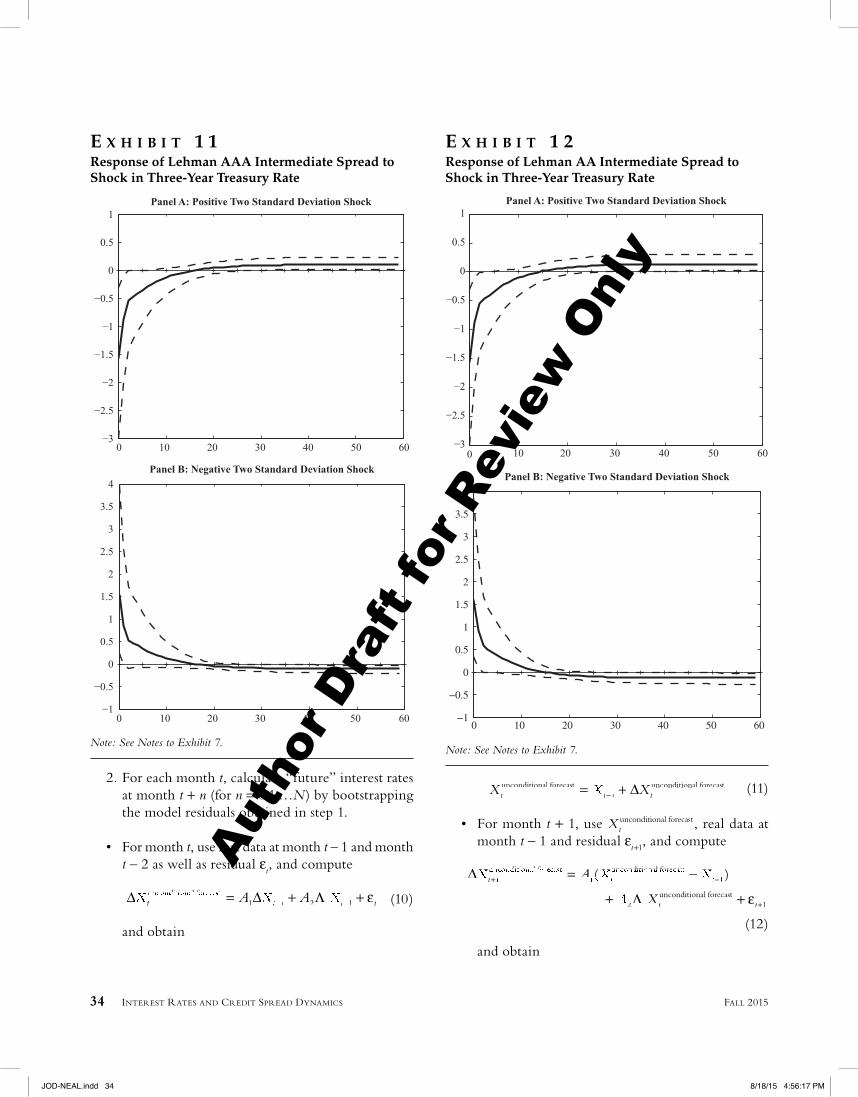
Notes: The graphs are obtained by constructing GIRFs that capture both the short-term dynamics and the long-run relationship between corporate and Treasury rates. The GIRFs are defined as the difference in month t + i between the conditional expectation of the corporate bond spread (cor-porate yield – Treasury yield) following a large shock to Treasury yields at month t and the conditional expectation across all possible shocks to Trea-sury yields. Both expectations condition on interest rates at t – 1. The solid line represents the average response of credit spreads, while the dashed lines show the 2.5th and 97.5th percentiles of the GIRF functions.


Auth

or D

raft

for R

evie

w O

nly


γγ

⎡

⎣⎢⎡⎡

⎢⎣⎣⎢⎢

⎤

⎦⎥⎤⎤

⎥⎦⎦⎥⎥ Π Λand so that2

1

22A A=

γ⎢⎢⎢ ⎥⎥⎥ Π =so that2

1 (8)

Models that include government rates are gener-alizations of the two-variable case.

1. Retrieve the f itted/realized residuals from the vector error-correction model for each month tusing actual data. In (2 × 2) matrix and (2 × 1)

vector notation, for month t, use real data at month t – 1 and month t – 2 and compute

where -

f t d1 1 2 1

1 2

A A X

X = X X-t t1A t

t t1 t

Δ =forecastedX forecasted Δ +X 1 ΛΔ

1 2

1 − (9)

in order to retrieve the (2 × 1) fitted residual vector ε = Δ − Δ forecastedX− Δt tΔ t

E X H I B I T 9Response of Lehman A Long Spread to Shock in 10-Year Treasury Rate


E X H I B I T 1 0Response of Lehman BAA Long Spread to Shock in 10-Year Treasury Rate



Auth

or D

raft

for R

evie

w O

nly


2. For each month t, calculate “future” interest rates at month t + n (for n = 0,1,…N ) by bootstrapping the model residuals obtained in step 1.

• For month t, use real data at month t – 1 and month t – 2 as well as residual ε

t, and compute

Δ = Δ + Λ + εditi l f t1−1Δ 2ΛA= A+t t1ΔA t t+ ε1− (10)

and obtain

+ Δ−unconditional forecast

1unconditional forecastX X=unconditional forecast Xt tX t

(11)

• For month t + 1, use unconditional forecastXt , real data at month t – 1 and residual ε

t+1, and compute

Δ =

+ Λ + ε−

+

( )−diti l f t

1unconditional forecast

1


1

A= −

XΛt t+ t

t t+ ε

(12)

and obtain

E X H I B I T 1 2Response of Lehman AA Intermediate Spread to Shock in Three-Year Treasury Rate


E X H I B I T 1 1Response of Lehman AAA Intermediate Spread to Shock in Three-Year Treasury Rate



Auth

or D

raft

for R

evie

w O

nly


+ Δ ++ Δunconditional forecast unconditional forecast1

unconditional forecastX X=+1unconditional forecast Xt t++ t

(13)

• For month t + n, n > 1, use + −1unconditional forecastXt n+ ,

+ −2unconditional forecastXt n+ and residual ε

t+n, and compute

Δ =

+ Λ + ε +

( )+ −diti l f t

1 1( −unconditional forecast


2 1+ −unconditional forecast

A= −+

XΛ2Λt n+ t n+++ t n++

t n+ t n+

(14)and obtain

+ Δ− ++ Δunconditional forecast unconditional forecast unconditional forecastX X=+unconditional forecast Xt n++ t n+ t n+

(15)

These forecasted interest rates are used to calcu-late the unconditional expectation of interest rate spreads.

3. For each month t, calculate “future” interest rates at time t + n for n = 0,1,…N by imposing that the value of the first residual at time t be larger than two standard deviations (for positive shocks).

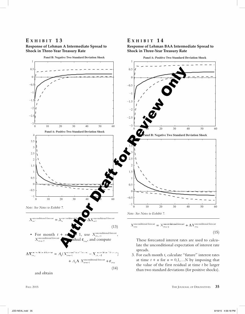
E X H I B I T 1 3Response of Lehman A Intermediate Spread to Shock in Three-Year Treasury Rate


E X H I B I T 1 4Response of Lehman BAA Intermediate Spread to Shock in Three-Year Treasury Rate



Auth

or D

raft

for R

evie

w O

nly


The remaining residual series is kept exactly the same as in step 2. The only difference between step 2 and step 3 is that in step 3 the first residual is drawn from the subset of residuals that are larger than two times the residuals’ standard deviation.

4. Record the corporate spread for both the uncon-ditional and the conditional simulation separately, and repeat steps 2 and 3 for the chosen number of simulations (1,000 in this case).

5. For a given number of steps ahead n, calculate the differences between these 1,000 simulated condi-tional and unconditional spreads and calculate their means, lower bounds, and upper bounds (2.5% and 97.5%, respectively).

6. For each number of steps ahead n, compute aver-ages of the means, lower bounds, and upper bounds across all t (months).

The Conditional Relationship between Credit Spreads and Treasury Rates

Exhibits 7 through 10 plot the response of long-term credit spreads to a two standard deviation shock in the 10-year Treasury rate. The exhibits plot the average response of credit spreads, as well as the 2.5th and 97.5th percentiles of the GIRF functions. In order to examine the long-run response, we plot the path of credit spreads for the five years that follow both a positive and a negative shock to the government rate. Although most empirical studies focus on the response of interest rates after a shock of one standard deviation, we focus on larger, two standard deviation shocks to government rates. Using such large shocks increases the power to reject the null hypothesis of no response to credit spreads following interest rate shocks.

As can been seen in the exhibits, there is no statisti-cally significant short-term reaction of spreads to either positive or negative shocks to long maturity government rates. After a large positive (negative) shock, the credit spread decreases (increases) initially but subsequently reverts to near pre-shock levels. However, this temporary average deviation from initial levels is generally not sta-tistically significantly different from zero, as shown by the width of the confidence bounds. In addition, across credit ratings, there is little difference in the response of credit spreads to interest rate shocks.

Exhibits 11 through 14 plot the response of intermediate-term corporate spreads to a two standard

deviation shock in the three-year Treasury rate, and as in the long-term rate cases, the short-run response of credit spreads to interest rate shocks are generally not statistically significantly different from zero, as shown by the width of the confidence bounds. For complete-ness, we also estimate (unreported) generalized impulse responses that include one-year government rates and find marginal significant response of intermediate matu-rity credit spreads. When the same impulse response analysis uses shocks that exceed one standard deviation, as is common in the empirical literature, we find no statistically significant relationship between shocks and future intermediate maturity credit spreads.

As a f inal robustness check, we also estimate a VECM that incorporates both short (three-month) and intermediate (three-year) government rates, and we again f ind no signif icant relationship between credit spreads and shocks to government rates, regardless of the maturity of the corporate bonds.

CONCLUSION

In contrast to existing studies, we find little evi-dence that unexpected changes to government rates lead to a significant change in future credit spreads. This empirical result holds for credit spreads constructed using bonds of differing maturities and credit ratings and is robust to shocks to both short and long maturity government bonds. This is in contrast to the existing literature, in which researchers have found that credit spreads and changes in rates are negatively correlated.

Our approach removes many of the restrictive assumptions found in the existing empirical literature. We use a vector error-correction methodology that allows for interest rates to be cointegrated, thus pre-cluding corporate and government rates from evolving in arbitrary, opposite directions over time. We also incorporate the empirical distribution of residuals when constructing the confidence intervals, thus allowing for potential fat tails in the distribution of interest rate shocks. Finally, our results condition on the prevailing interest rate environment, which may be viewed as a proxy for economic conditions. The absence of a mean-ingful relationship between interest rates and credit spreads provides empirical evidence against the dynamic process for credit spreads assumed in existing structural models for pricing corporate bonds.


Auth

or D

raft

for R

evie

w O

nly


ENDNOTES

We thank Rob Bliss, Jin-Chuan Duan, Greg Duffee, Rob Engle, Jean Helwege, Mike Hemler, Bob Jarrow, Brad Jordan, Avi Kamara, Jon Karpoff, Sharon Kozicki, Paul Malatesta, Rich Rodgers, Sergei Sarkissian, Pu Shen, Richard Shockley, Art Warga, Eric Zivot, two anonymous referees, and the seminar participants at Indiana University, Federal Reserve Bank of Kansas City, Bank of International Settlements, Loyola University in Chicago, University of Kentucky, University of Melbourne, University of Sydney, the 9th Annual Derivatives Securities Conference, and the American Finance Association annual conference. We also thank Klara Parrish and Isaac Wang for research assistance. An earlier version of this article was titled “Credit Spreads and Interest Rates: A Cointegration Approach.”

1See Black and Cox [1976], Leland [1994], Collin- Dufresne and Goldstein [2001], Eom et al. [2004], Schaefer and Strebulaev [2008], and Ericsson et al. [2009].

2Although cointegration is intuitively appealing, it assumes that the underlying variables are nonstationary. We impose the assumption of unit root processes not because we believe that interest rates can exhibit unbounded varia-tion, but because it provides the distribution theory that best represents the finite sample properties of our data. Our view is consistent with that of Granger and Swanson [1996] and Phillips [1998], who showed that nonstationary distribution models provide superior inference for both unit root and near unit root processes.

3For instance, see Fama and French [1989], Chan-Lau and Ivaschenko [2001, 2002], Davies [2008], and Mueller [2009].

4See Rose [1988], Stock and Watson [1988], Hall et al. [1992], Bradley and Lumpkin [1992], Konishi et al. [1993], and Enders and Granger [1998] for short-term rates; Mehra [1994] and Campbell and Shiller [1987] for long-term rates.

5Although cointegration is intuitively appealing, it assumes that the underlying variables are nonstationary. We impose the assumption of unit root processes not because we believe that interest rates can exhibit unbounded varia-tion, but because it provides the distribution theory that best represents the finite sample properties of our data. Our view is consistent with Granger and Swanson [1996] and Phillips [1998] who showed that nonstationary distribution models provide superior inference for both unit root and near-unit root processes.

6An attractive feature of the cointegration framework is that it allows one to distinguish between short-run and long-run behavior. We estimate the models with a two-stage procedure that first identifies the cointegration vector, and then includes the vector in a second-stage regression of changes in corporate rates on changes in Treasury rates.

7For purposes of comparing across models, we fix the number of lags for changes in rates to one, which implies that there are two lags in the levels. We also consider other forms as a robustness check where we select variable lags with Akaike’s information criterion, and our results remain the same.

REFERENCES

Avramov, D., T. Chordia, G. Jostova, and A. Philipov. “Momentum and Credit Rating.” Journal of Finance, Vol. 62, No. 5 (2007), pp. 2503-2520.

Batten, J.A., W.P. Hogan, and G. Jacoby. “Measuring Credit Spreads: Evidence from Australian Eurobonds.” Applied Financial Economics, Vol. 15, No. 9 (2005), pp. 651-666.

Black, F., and J.C. Cox. “Valuing Corporate Securities: Some Effects of Bond Indenture Provisions.” Journal of Finance, Vol. 31, No. 2 (May 1976), pp. 351-367.

Black, F., and M. Scholes. “The Pricing of Options and Cor-porate Liabilities.” Journal of Political Economy, Vol. 81, No. 3 (May/June 1973), pp. 637-654.

Bradley, M., and S. Lumpkin. “The Treasury Yield Curve as a Cointegrated System.” Journal of Financial and Quantitative Analysis, 27 (1992), pp. 449-464.

Campbell, J.Y., and R.J. Shiller. “Cointegration and Tests of Present Value Models.” Journal of Political Economy, Vol. 95, No. 5 (October 1987), pp. 1062-1088.

Campbell, J.Y., and G.B. Taksler. “Equity Volatility and Corporate Bond Yields.” Journal of Finance, Vol. 58, No. 6 (December 2003), pp. 2321-2349.

Chan-Lau, J., and I. Ivaschenko. “Corporate Bond Risk and Real Activity: An Empirical Analysis of Yield Spreads and Their Systematic Components.” IMF Working Paper 01/158, 2001.

——. “The Corporate Spread Curve and Industrial Production in the United States.” IMF Working Paper 02/8, 2002.

Collin-Dufresne, P., and R. Goldstein. “Do Credit Spreads Ref lect Stationary Leverage Ratios?” Journal of Finance, Vol. 56, No. 5 (October 2001), pp. 1929-1957.

Collin-Dufresne, P., R.S. Goldstein, and J.S. Martin. “The Determinants of Credit Spread Changes.” Journal of Finance, Vol. 56, No. 6. (December 2001), pp. 2177-2207.


Auth

or D

raft

for R

evie

w O

nly


Davies, A. “Credit Spread Determinants: An 85 Year Per-spective.” Journal of Financial Markets, Vol. 11, No. 2 (2008), pp. 180-197.

Duan, J.-C., and S.R. Pliska. “Option Valuation with Co-Integrated Asset Prices.” Journal of Economic Dynamics and Con-trol, Vol. 28, No. 4 ( January 2004), pp. 727-754.

Duffee, G.R. “Treasury Yields and Corporate Bond Yield Spreads: An Empirical Analysis.” Journal of Finance, Vol. 53, No. 6 (1998), pp. 2225-2242.

Enders, W., and C.W.J. Granger. “Unit-Root Tests and Asymmetric Adjustment with an Example Using the Term Structure of Interest Rates.” Journal of Business and Economic Statistics, Vol. 16, No. 3 (February 1998), pp. 304-311.

Eom, Y.H., J. Helwege, and J.-Z. Huang. “Structural Models of Corporate Bond Pricing: An Empirical Analysis.” Review of Financial Studies, Vol. 17, No. 2 (2004), pp. 499-544.

Ericsson, J., K. Jacobs, and R. Oviedo. “The Determinants of Credit Default Swap Premia.” Journal of Financial and Quantita-tive Analysis, Vol. 44, No. 1 (Feb. 2009), pp. 109-132.

Fama, E., and K.R. French. “Business Conditions and Expected Returns on Stocks and Bonds.” Journal of Financial Economics, Vol. 25, No. 1 (November 1989), pp. 23-49.

Gilchrist, S., V. Yankov, and E. Zakrajsek. “Credit Market Shocks and Economic Fluctuations: Evidence from Corporate Bond and Stock Markets.” Journal of Monetary Economics, Vol. 56, No. 4 (2009), pp. 471-493.

Goldstein, R., N. Ju, and H. Leland. “An EBIT-Based Model of Dynamic Capital Structure.” Journal of Business, Vol. 74, No. 4 (2001), pp. 483-512.

Granger, C.W.J., and P. Newbold. “Spurious Regressions in Econometrics.” Journal of Econometrics, Vol. 2, No. 2 (1974), pp. 111-120.

Granger, C.W.J., and N.R. Swanson. “Future Developments in the Study of Cointegrated Variables.” Oxford Bulletin of Economics and Statistics, Vol. 58, No. 3 (1996), pp. 537-553.

Hall, A.D., H.M. Anderson, and C.W.J. Granger. “A Cointe-gration Analysis of Treasury Bill Yields.” Review of Economics and Statistics, Vol. 74, No. 1 (1992), pp. 116-126.

Jacoby, G., R.C. Liao, and J.A. Batten. “Testing for the Elasticity of Corporate Yield Spreads.” Journal of Finan-cial and Quantitative Analysis, Vol. 44, No. 3 ( June 2009), pp. 641-656.

Johansen, S. “Statistical Analysis of Cointegrating Vectors.” Journal of Economic Dynamics and Control, Vol. 12 No. 2/3 (1988), pp. 231-254.

Kim, J., K. Ramaswamy, and S. Sundaresan. “Does Default Risk in Coupons Affect the Valuation of Corporate Bonds? A Contingent Claims Model.” Financial Management, Vol. 22, No. 3 (1993), pp. 117-131.

Konishi, T., V. Ramey, and C.W.J. Granger. “Stochastic Trends and Short-Run Relationships Between Financial Variables and Real Activity.” National Bureau of Economic Research Working Paper 4275, 1993.

Koop, G., M.H. Pesaran, and S.M. Potter. “Impulse Response Analysis in Nonlinear Multivariate Models.” Journal of Econo-metrics, Vol. 74, No. 1 (1996), pp. 119-147.

Leland, H.E. “Corporate Debt Value, Bond Covenants, and Optimal Capital Structure.” Journal of Finance, Vol. 49, No. 4 (September 1994), pp. 1213-1252.

Leland, H.E., and K. Toft. “Optimal Capital Structure, Endogenous Bankruptcy, and the Term Structure of Credit Spreads.” Journal of Finance, Vol. 51, No. 3 (1996), pp. 987-1020.

Longstaff, F.A., and E. S. Schwartz. “A Simple Approach to Valuing Risky Fixed and Floating Rate Debt.” Journal of Finance, Vol. 50, No. 3, ( July 1995), pp. 789-820.

——. “Valuing Credit Derivatives.” The Journal of Fixed Income, Vol. 5, No. 1 ( Jan. 1995), pp. 6-12.

MacKinnon, J.G. “Critical Values for Cointegration Tests.” R.F. Engle and C.W.J. Granger, eds., Long-Run Economic Rela-tionships: Readings in Cointegration. Oxford University Press, 1991, pp. 267-276.

Mehra, Y. “An Error-Correction Model of the Long-Term Bond Rate.” Federal Reserve Bank of Richmond Economic Quar-terly, Vol. 80, No. 4 (1994), pp. 49-67.


Auth

or D

raft

for R

evie

w O

nly


Merton, R.C. “On the Pricing of Corporate Debt: The Risk Structure of Interest Rates.” Journal of Finance, Vol. 29, No. 2 (May 1974), pp. 449-470.

Mueller, P. “Credit Spreads and Real Activity.” Working paper, London School of Economics and Political Science, 2009.

Pesaran, M.H., and S.M. Potter. “A Floor and Ceiling Model of U.S. Output.” Journal of Economic Dynamics and Control, Vol. 21, No. 4-5 (1997), pp. 661-695.

Phillips, P. “Impulse Response and Forecast Error Variance Asymptotics in Nonstationary VARs.” Journal of Econometrics, Vol. 83, No. 1-2 (1998), pp. 21-56.

Rose, A. “Is the Real Interest Rate Stable?” Journal of Finance, Vol. 43, No. 5 (1988), pp. 1095-1112.

Schaefer, S,M., and I.A. Strebulaev. “Structural models of Credit Risk Are Useful: Evidence from Hedge Ratios on Corporate Bonds.” Journal of Financial Economics, Vol. 90, No. 1 (2008), pp. 1-19.

Stock, J.H., and M.W. Watson. “Testing for Common Trends.” Journal of the American Statistical Association, Vol. 83, No. 404 (December 1988), pp. 1097-1107.

To order reprints of this article, please contact Dewey Palmieri at [email protected] or 212-224-3675.


Auth

or D

raft

for R

evie

w O

nly

Date post:	29-Apr-2018
Category:	Documents
Upload:	phungdang
View:	217 times
Download:	1 times

Interest Rates and Credit Spread Dynamicsfaculty.fiu.edu/~dupoyetb/credit_spreads.pdfFALL 2015 THE...

Documents