INTERFERENCE OF HYDRAULIC ROUGHNESS GENERATED...

YURI JACQUES AGRA BEZERRA DA SILVA

INTERFERENCE OF HYDRAULIC ROUGHNESS GENERATED BY

UNSUBMERGED VEGETATION ON SEDIMENT TRANSPORT IN

CAPIBARIBE RIVER

RECIFE - PE

2012

ii


INTERFERENCE OF HYDRAULIC ROUGHNESS GENERATED BY


CAPIBARIBE RIVER

RECIFE-PE

2012

Dissertation presented to Rural Federal

University of Pernambuco, as part of the

demanding of Graduate Program in Soil Science

to obtain the Master Degree.

Adviser

Prof. José Ramon Barros Cantalice, Dr

iii


TITLE: INTERFERENCE OF HYDRAULIC ROUGHNESS GENERATED BY


CAPIBARIBE RIVER.

Approved on January 6, 2012.

_______________________________________

Prof. Dr. Brivaldo Gomes de Almeida (Examiner)

_______________________________________

Prof. Dr. Vicente de Paula Silva (Examiner)

_______________________________________

Prof. Dr. Moacyr Cunha Filho (Examiner)

_______________________________________

Prof. Dr. José Ramon Barros Cantalice (Adviser)

iv

“Aprendi que os sonhos transformam a vida numa grande aventura.

Eles não determinam o lugar aonde você vai chegar, mas produzem

a força necessária para arrancá-lo do lugar em que você está.”

(Augusto Cury)

v

God, by giving me health to complete my research;

My grandmother: Zene dos Anjos Bezerra da Silva;

My mother and father: Vilma Agra da Fonseca and Roberto Jacques Bezerra da Silva;

My brother and sister: Ygor Jacques Agra Bezerra da Silva and Rayanna Jacques Agra Bezerra da Silva;

My fiancee: Cinthia Maria Cordeiro Atanázio Cruz;

All people who contributed with my Dissertation.

DEDICATE

vi

ACKNOWLEDGEMENTS

I would like to express my sincere gratitude to:

God by giving me health for developing this research and help me to overcome

all challenges in my life;

Rural Federal University of Pernambuco by the opportunity of carrying out the

master's degree in the soil science program;

My adviser Dr. José Ramon Barros Cantalice, for the opportunity and guidance;

My colleagues and friends in the Soil Conservation Engineering Laboratory by

the spirit of group, in particular Cícero Gomes dos Santos, Douglas Monteiro

Cavalcante, João Victor Ramos de Alexandre, Leidivam Vieira, Luiz Antônio de

Almeida Neto, Rogério Oliveira de Melo, Victor Casimiro Piscoya and Wagner

Luís da Silva Souza, for the help in field measurements;

My fiancee Cinthia Maria Cordeiro Atanázio Cruz, who was fundamental during

the direct measurement campaigns, taking notes in the field and being helpful in

the analysis at Soil Conservation Engineering Laboratory;

My brother and best friend Ygor Jacques Agra Bezerra da Silva for his

friendship and precious advices;

The Professors in the PPGCS represented by Brivaldo Gomes de Almeida,

Clístenes Williams Araújo do Nascimento, Izabel Cristina de Luna Galindo,

Mateus Rosas Ribeiro, Mateus Rosas Ribeiro Filho, Maria Betânia Galvão dos

Santos Freire, Mário de Andrade Lira Júnior, Sheila Maria Bretas Bittar

Schulze, Valdomiro Severino de Souza Júnior and also the Agronomic Engineer

José Fernando Wanderley Fernandes Lima (Zeca);

The Professor Luciana of Brazil Canada Center;

Also, I would like to thank Maria do Socorro Santana and Josué by solving

several troubles in the coordination as well as the happiness during the time

job;

vii

I would like to thank the support from my family, in particular my mother Vilma

Agra da Fonseca and my grandmother Zene dos Anjos for their

encouragement, chiefly during the difficult moments;

The National Council for Scientific and Technological Development (CNPq),

which provided the development of this research;

Finally, I would like to extend my acknowledgment for all who contributed in

several ways towards the success of this Dissertation.

viii

CONTENTS

ACKNOWLEDGEMENTS .................................................................................. vi

CONTENTS ..................................................................................................... viii

LIST OF FIGURES ............................................................................................. x

LIST OF TABLES .............................................................................................. xii

LIST OF SIMBOLS .......................................................................................... xiii

LIST OF ABBREVIATIONS ............................................................................. xiv

RESUMO .......................................................................................................... xv

ABSTRACT ...................................................................................................... xvi

1. LITERATURE REVIEW ................................................................................ 1

1.1. Importance of sediment transport in watersheds ...................................... 1

1.2. Suspended sediment and bedload transport ............................................ 2

1.3. Impact of vegetation on sediment transport .............................................. 5

1.4. Flow resistance and vegetation ................................................................ 6

1.4.1. Conventional resistance coefficients .................................................. 7

1.4.2. Drag coefficient, plant Reynolds number and vegetation resistance

force ............................................................................................................. 8

2. OBJECTIVES ............................................................................................. 12

3. HYPOTHESIS ............................................................................................ 12

4. MATERIALS AND METHODS .................................................................... 13

4.1. Study area description ............................................................................ 13

4.2. Physical-hydric characteristics of Capibaribe Watershed ....................... 14

4.3. Crosses sections and direct measurement campaigns ........................... 15

4.4. Velocity measurement. ........................................................................... 16

4.5. Water discharge measurement ............................................................... 17

4.6. Suspended sediment sampling ............................................................... 18

4.7. Bedload discharge and particle size distribution ..................................... 21

4.8. Hydraulic characteristics and vegetation resistance parameters ............ 23

4.9. Description and structural parameters of vegetation............................... 24

4.10. Statistical analysis ................................................................................ 25

ix

5. RESULTS AND DISCUSSION ................................................................... 25

5.1. Rainfall in Capibaribe River .................................................................... 25

5.2. Hydraulic characteristics and rating curve of Capibaribe River ............... 26

5.3. Suspended and bedload transport for crosses sections under

nonvegetated conditions ................................................................................ 28

5.4. Interference of unsubmerged vegetation on sediment transport of

Capibaribe watershed .................................................................................... 31

5.5. Multivariate analysis ............................................................................... 35

5.6. Principal component analysis ................................................................. 35

5.7. Hierarchical cluster analysis ................................................................... 37

6. CONCLUSIONS ......................................................................................... 40

7. REFERENCES ........................................................................................... 41

x

LIST OF FIGURES

Figure 1. Sampled and unsampled zone of each vertical in Capibaribe

watershed (Edwards and Glysson, 1999). ……………………………………...…2

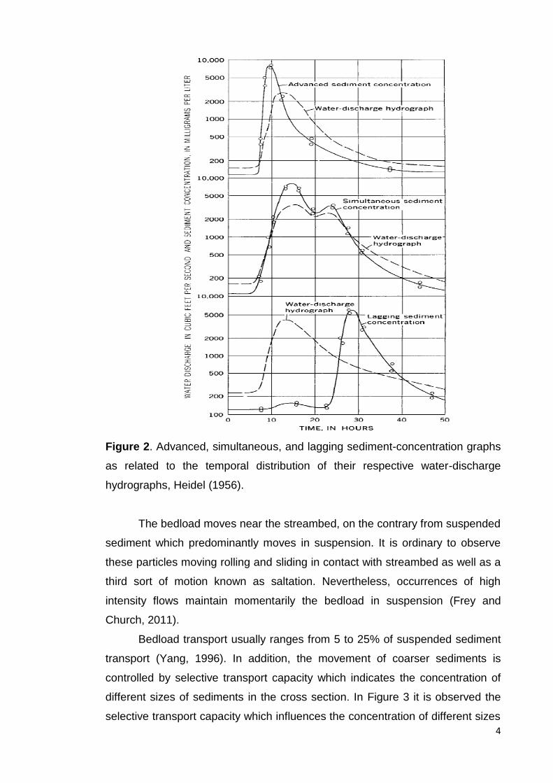
Figure 2. Advanced, simultaneous, and lagging sediment-concentration graphs

as related to the temporal distribution of their respective water-discharge

hydrographs (Heidel, 1956). ………………………………………………………....4

Figure 3. Discharge-weighted concentration of suspended sediment for different

particle-size groups at a sampling vertical in the Missouri River at Kansas City.5

Figure 4. Location of Capibaribe watershed and its major watercourse in

Pernambuco state map (ANA, 2010). ……………………………………………..13

Figure 5. Location of crosses sections in Capibaribe River……………………..16

Figure 6. Rotating-element current meter used in Capibaribe River. …….....…17

Figure 7. Suspended sediment sampling (sampler - US DH-48) in Capibaribe

River. ……….………………………………………………………………………....19

Figure 8. Equal-width-increment vertical transit rate relative to sample volume,

which is proportional to water discharge at each vertical. …………………...….20

Figures 9. Bedload sampling with the sampler US BLH – 84 model………...…22

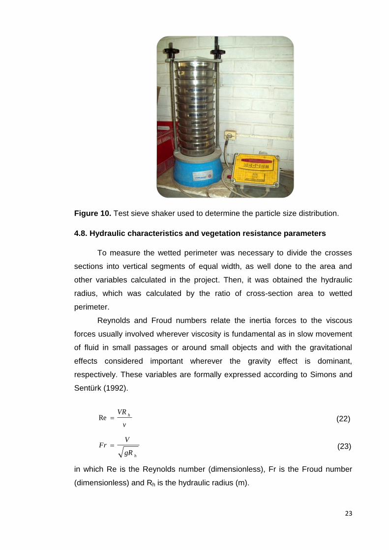
Figure 10. Test sieve shaker used to determine the particle size distribution.

…………………………………………………………………………......................23

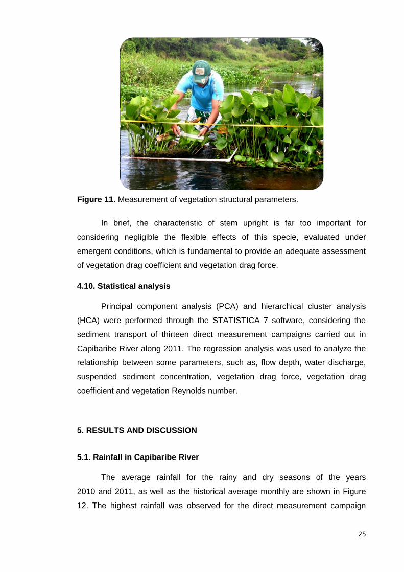
Figure 11. Measurement of vegetation structural parameter………….…...……25

Figure 12. Distribution of average annual rainfall for non-rainy and rainy 2010

and 2011, as well as the historical average in Capibaribe River (LAMEPE,

2011). ………………………………………………………………………………...26

Figure 13. Particle size distribution curve of sediment transported in the

streambed by Capibaribe River in 29/05/2011. ………………………..………...27

xi

Figure 14. Rating curve of directing measurement campaigns performed under

nonvegetated conditions in Capibaribe River…..……………………...….…..….28

Figure 15. Sediment rating curve of Capibaribe River with instantaneous

sediment concentration. …………………………………………...………………..30

Figure 16. Suspended sediment rating curve of Capibaribe watershed. …...…31

Figure 17. Comparison between crosses sections under absence and presence

of unsubmerged vegetation. ………………………………………………....…….32

Figure 18. Relationship between the individuals’ values of CD’ and (VRh)….…33

Figure 19. Drag coefficient of Echinodorus macrophyllus in function of plant

Reynolds number for the flow evaluated in Capibaribe River. ……….…………34

Figure 20. Relationship between drag force, shear stress reduction and bedload

reduction during vegetated and unvegetated period. …………………………....35

Figure 21. Projection of the variables on the factor-plane. …………………...…37

Figure 22. Dendrogram of classification for the thirteen direct measurement

campaigns. .……………………………………….…………………………….……39

xii

LIST OF TABLES

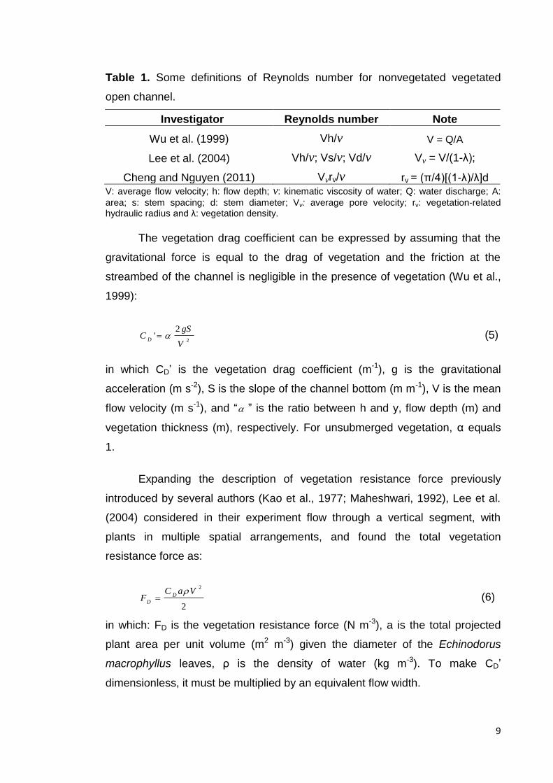
Table 1. Several definitions of Reynolds number for nonvegetated and

vegetated open channel………………………………………………………………9

Table 2. Predominance of some classes of soils in Capibaribe watershed

(USDA, 1999). ………..………………………………………………………….….14

Table 3. Physical-hydric characteristics of the Capibaribe watershed..……..…15

Table 4. Measurement of average flow velocity according to flow

depth…………………………………………………………………………………..17

Table 5. Hydraulic variables of direct measurements campaigns performed

under nonvegetated conditions in Capibaribe River. ………….………………...27

Table 6. Sediment transport variables of directing measurement campaigns

performed in the crosses sections under nonvegetated conditions. ………......29

Table 7. Principal components loadings, eigenvalues and explained variance of

six components obtained for all direct measurement campaigns performed in

Capibaribe River. ……….…………………………………………………….……..36

xiii

LIST OF SIMBOLS A = watershed area; α = total projected plant area per unit volume; Ai = influence area of the vertical segment; Ap = total area projected with plant; B = bottom of the River; BC = Box Coefficient; CD’ = vegetation drag coefficient; CDv = drag coefficient (dimensionless); d = stem diameter; D = distance between crosses sections; Dl = leaf diameter; d50 = median grain diameter; FD = vegetation resistance force; Fr = Froud number; fv = vegetation friction factor; g = gravitational acceleration; h = flow depth; K = constant of variable proportionality; Kf = form coefficient; L = length of the main watercourse; Lx = equivalent width; M = suspended sediment mass; m = mass of sediment from bedload transport; n = Manning’s coefficient; n’ = Manning’s coefficient due to grain roughness; n’’ = Manning’s coefficient due to form roughness; nb = Manning coefficient for unsubmerged vegetation; Pw = wetted perimeter; Q = water discharge; QB = bedload discharge; Qi = water discharge in each vertical segment; Re = Reynolds number; Replant = plant Reynolds number; Rh = hydraulic radius; Rv = vegetation Reynolds number; rv = vegetation-related hydraulic radius; S = slope of the channel bottom; s = stem spacing; Sf = surface flow; SSC = suspended sediment concentration;

SSC = average of suspended sediments concentration;

SSCi = suspended sediment concentration at each vertical; SSQ = suspended solid discharge; Sw = water line slope; T = temperature in degrees Celsius; t1 = minimum time of the suspended sediment sampling; t2 = sampling time of bedload transport; V = average flow velocity; Vi = average flow velocity in the sampled vertical segment; Volsample = sample volume; Vt = transit rate; Vv = average pore velocity;

v = kinematic viscosity of water;

w = width of nozzle (US BLH – 84); = relation between flow depth and vegetation thickness;

ρ = density of water; λ = factor of vegetation density;

τ = shear stress;

xiv

LIST OF ABBREVIATIONS

ANA - Brazilian National Water Agency

CNPq - Brazilian National Council for Scientific and Technological

USDA - U.S. Department of Agriculture

PE – Pernambuco state

EWI - Equal Width Increment

PCA - Principal Component Analysis

HCA - Hierarchical Cluster Analysis

DH - Depth Hand

BLH - Bedload Hand

CPRH - State Agency of Environment

RMR - Metropolitan Region of Recife

SUDENE - Superintendence of Northeast Development

USGS - United State Geological Survey

LAMEPE - Meteorological Laboratory of Pernambuco

xv

RESUMO

A vegetação desempenha um papel importante nos processos de transporte de

sedimentos, sendo essencial melhorar o conhecimento sobre a interferência da

vegetação emersa neste processo. Dessa maneira, o principal objetivo desta

pesquisa foi avaliar a interferência da rugosidade hidráulica gerada pela

vegetação emersa no transporte de sedimentos, com base na relação entre o

coeficiente de arraste vegetal (CD’) e o número de Reynolds da planta (Replanta)

do Rio Capibaribe. Campanhas de medição direta foram realizadas seguindo a

metodologia de amostragem por igual incremento de largura (IIL), usando o

amostrador US DH-48 para amostragem de sedimento em suspensão e o

amostrador US BLH 84 para amostragem de sedimento de fundo. Foi avaliada

a resistência gerada pela espécie Echinodorus macrophyllus por meio do

coeficiente de arraste vegetal (CD’) e da força de arraste vegetal (FD), bem

como a influência destes parâmetros no transporte de sedimentos da bacia

hidrográfica do rio Capibaribe. Além disso, foram realizadas análise de

componentes principais (ACP) e análise de agrupamento hierárquico (ACH)

para escolher as variáveis mais importantes associadas ao transporte de

sedimentos e classificar as treze campanhas de medição direta em grupos de

acordo com a similaridade, respectivamente. O CD’ atingiu um valor máximo

igual a 11,13 m-1, indicando a resistência hidráulica gerada pela Echinodorus

macrophyllus. Os dois primeiros componentes extraídos tiveram autovalores

iguais a 6,74 e 3,15, representando 90,03% da variância total explicada. A ACH

revelou cinco grupos em que o segundo foi formado pelas campanhas de

medição direta realizadas com vegetação emersa ao longo da seção

transversal (C2, C4 e C6). Estas medições apresentaram os valores mais

baixos, sobretudo para a tensão de cisalhamento e descarga sólida de fundo.

O último grupo foi formado pelas campanhas de medição direta (C10, C11, C12

e C13), que reuniram principalmente os maiores valores para o raio hidráulico,

vazão, descarga sólida de fundo e tensão de cisalhamento. Sendo assim, a

análise multivariada foi considerada uma ferramenta adequada para avaliar a

influência da vegetação emersa no transporte de sedimentos da bacia

hidrográfica do rio Capibaribe.

Palavras-chave: coeficiente de arraste vegetal, análise de agrupamento

hierárquico e análise de componentes principais.

xvi

ABSTRACT

The vegetation plays an important role on sediment transport processes, being

essential to improve the knowledge regarding the unsubmerged vegetation

interference in this process. Thus, the main aim of this research was to assess

the hydraulic roughness interference generated by unsubmerged vegetation on

sediment transport, based on relationship between vegetation drag coefficient

(CD’) and Reynolds number of vegetation (Replant) from Capibaribe River. Direct

measurements campaigns were carried out according to the equal-width-

increment (EWI), using the US DH-48 sampler to suspended sediment sampling

and US BLH 84 sampler to bedload sampling. It was evaluated the resistance

generated by Echinodorus macrophyllus by means of the vegetation drag

coefficient (CD’) and vegetation drag force (FD) as well as the influence of these

parameters on sediment transport of Capibaribe watershed. Furthermore,

principal component analysis (PCA) and hierarchical cluster analysis (HCA)

were performed to choose the most important variables associated with the

sediment transport and classify the thirteen direct measurement campaigns in

groups according to the similarity, respectively. The CD’ reached a maximum

value equal to 11.13 m-1, indicating the hydraulic resistance generated by

Echinodorus macrophyllus. The first two components extracted had eigenvalues

equal to 6.74 and 3.15, accounting for the 90.03% of the total variance

explained. The HCA revealed five clusters in which the second was formed by

the direct measurement campaigns carried out with unsubmerged vegetation

along the cross section (C2, C4 and C6). These measurements showed the

lowest values, chiefly to the shear stress and bedload discharge. The last

cluster was formed by the direct campaigns (C10, C11, C12 and C13) which

mainly gathered the largest values of hydraulic radius, water discharge, bedload

discharge and shear stress. As a result, the multivariate analysis was

considered an adequate tool for evaluating the interference of unsubmerged

vegetation on sediment transport of Capibaribe watershed.

Keywords: vegetation drag coefficient, hierarchical cluster analysis and

principal component analysis.

1

1. LITERATURE REVIEW

1.1. Importance of sediment transport in watersheds

The sediment transport researches are way too important in several

aspects. The sustainability of watersheds is strictly associated with sediment

transport along their watercourses in which excessive sediment fluxes

generated by extreme flows can destabilize River channels. As a result,

provokes damages to property and also public structure, narrows down the

quality of water as well as increases flooding problems (Frey and Church,

2011). Therefore, it is fundamental go into more depth for learning to deal with

this complex scientific trouble.

In addition, comprehension regarding sediment transport in watersheds

is useful for providing an adequate management of streams and reservoirs.

Data on amount of sediment which has been transported by Rivers is essential

in the planning of hydraulic structures, such as, dams and irrigations channels,

as well as the features and amount of sediment transported from the drainage

basins provides information to predict stream changes (Edwards and Glysson,

1999).

Several cities were originated on the banks of Rivers, mainly because

water resources contribute to the development of the area under its influence.

Recife is one of these cities which had the formation and expansion influenced

by Capibaribe River, the major water resource of the city (Mayrinck, 2003).

Moreover, this River has a historical and economic importance for Pernambuco

state (Brazil), where has been developing activities associated with sugar-cane

industry. In spite of the importance of Capibaribe River, responsible by the

water supply of several cities, a portion localized in low Capibaribe – Recife was

classified as polluted water. Furthermore, the estuary has been suffering due to

anthropogenic activities (CPRH, 2006).

There are several problems related with sediment transport in

watersheds. For instance: increases the cost of water treatment; modifies the

size of channel; acts as a carrier of bacteria and viruses; increases the transport

of pollutants, chiefly the cohesive sediment; narrows down the flow depth,

damaging the sea transport and increasing the possibility of floods. On the other

2

hand, there are not only damages but also benefits associated with sediment

transport. For example: decreases the erosion action of water in River runoff;

improves the quality of water due to reduction of some pollutants; allows the

chemistry reactions on sediment surface; carries organic matter, improving the

aquatic life for some microorganisms (Carvalho, 2008).

1.2. Suspended sediment and bedload transport

First of all, sediment transport in watersheds is classified into two groups,

such as, suspended and bedload transport. Suspended sediment is a term

applied to particles which are maintained suspended by the vertical component

of velocity in turbulent flux while is transported by the horizontal component of

velocity in the same flux. Furthermore, the suspended sediment transport is

chiefly governed by the flow velocity, whilst the coarsest sediments might move

only occasionally and remain at rest much of the time (Edwards and Glysson,

1999).

The objective of suspended sediment sampler is to acquire a

representative sample of the water sediment mixture moving in the stream. It is

essential to carry out an isokinetic and point-integrating suspended sediment

sampling in which each vertical along the cross section presents two zones,

sampled and unsampled (Figure 1). Furthermore, depending on velocity and

flow turbulence the amount suspended sediment moving in the verticals may

represent or not the large portion of the total suspended sediment (Edward and

Glysson, 1999).

Figure 1. Sampled and unsampled zone of each vertical in Capibaribe

watershed (Edwards and Glysson, 1999).

3

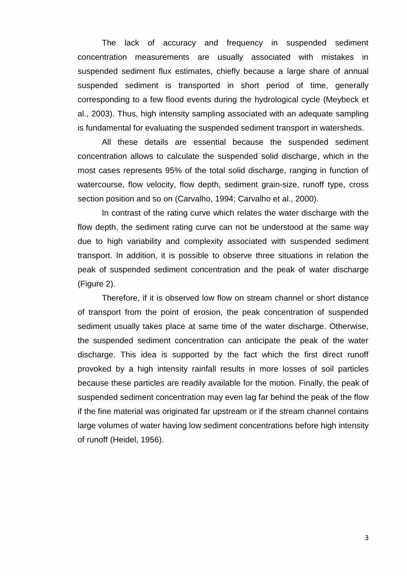
The lack of accuracy and frequency in suspended sediment

concentration measurements are usually associated with mistakes in

suspended sediment flux estimates, chiefly because a large share of annual

suspended sediment is transported in short period of time, generally

corresponding to a few flood events during the hydrological cycle (Meybeck et

al., 2003). Thus, high intensity sampling associated with an adequate sampling

is fundamental for evaluating the suspended sediment transport in watersheds.

All these details are essential because the suspended sediment

concentration allows to calculate the suspended solid discharge, which in the

most cases represents 95% of the total solid discharge, ranging in function of

watercourse, flow velocity, flow depth, sediment grain-size, runoff type, cross

section position and so on (Carvalho, 1994; Carvalho et al., 2000).

In contrast of the rating curve which relates the water discharge with the

flow depth, the sediment rating curve can not be understood at the same way

due to high variability and complexity associated with suspended sediment

transport. In addition, it is possible to observe three situations in relation the

peak of suspended sediment concentration and the peak of water discharge

(Figure 2).

Therefore, if it is observed low flow on stream channel or short distance

of transport from the point of erosion, the peak concentration of suspended

sediment usually takes place at same time of the water discharge. Otherwise,

the suspended sediment concentration can anticipate the peak of the water

discharge. This idea is supported by the fact which the first direct runoff

provoked by a high intensity rainfall results in more losses of soil particles

because these particles are readily available for the motion. Finally, the peak of

suspended sediment concentration may even lag far behind the peak of the flow

if the fine material was originated far upstream or if the stream channel contains

large volumes of water having low sediment concentrations before high intensity

of runoff (Heidel, 1956).

4

Figure 2. Advanced, simultaneous, and lagging sediment-concentration graphs

as related to the temporal distribution of their respective water-discharge

hydrographs, Heidel (1956).

The bedload moves near the streambed, on the contrary from suspended

sediment which predominantly moves in suspension. It is ordinary to observe

these particles moving rolling and sliding in contact with streambed as well as a

third sort of motion known as saltation. Nevertheless, occurrences of high

intensity flows maintain momentarily the bedload in suspension (Frey and

Church, 2011).

Bedload transport usually ranges from 5 to 25% of suspended sediment

transport (Yang, 1996). In addition, the movement of coarser sediments is

controlled by selective transport capacity which indicates the concentration of

different sizes of sediments in the cross section. In Figure 3 it is observed the

selective transport capacity which influences the concentration of different sizes

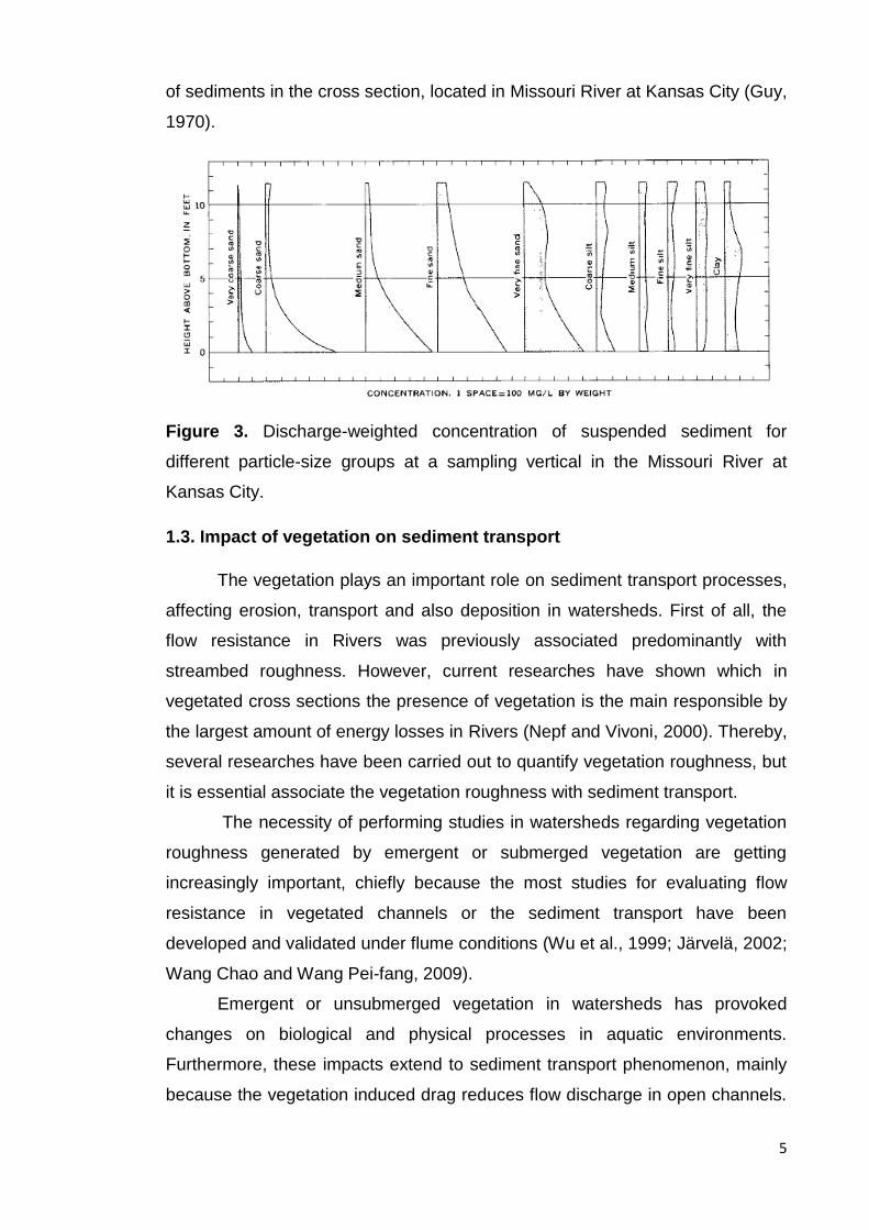
5

of sediments in the cross section, located in Missouri River at Kansas City (Guy,

1970).

Figure 3. Discharge-weighted concentration of suspended sediment for

different particle-size groups at a sampling vertical in the Missouri River at

Kansas City.

1.3. Impact of vegetation on sediment transport

The vegetation plays an important role on sediment transport processes,

affecting erosion, transport and also deposition in watersheds. First of all, the

flow resistance in Rivers was previously associated predominantly with

streambed roughness. However, current researches have shown which in

vegetated cross sections the presence of vegetation is the main responsible by

the largest amount of energy losses in Rivers (Nepf and Vivoni, 2000). Thereby,

several researches have been carried out to quantify vegetation roughness, but

it is essential associate the vegetation roughness with sediment transport.

The necessity of performing studies in watersheds regarding vegetation

roughness generated by emergent or submerged vegetation are getting

increasingly important, chiefly because the most studies for evaluating flow

resistance in vegetated channels or the sediment transport have been

developed and validated under flume conditions (Wu et al., 1999; Järvelä, 2002;

Wang Chao and Wang Pei-fang, 2009).

Emergent or unsubmerged vegetation in watersheds has provoked

changes on biological and physical processes in aquatic environments.

Furthermore, these impacts extend to sediment transport phenomenon, mainly

because the vegetation induced drag reduces flow discharge in open channels.

6

As a result, increasing flood attenuation and also sediment deposition (Cheng

and Nguyen, 2011).

In addition, the bedload transport capacity decreases concurrently with

the increases of flow resistance generated by vegetation on the watercourses.

Thereby, the diameter and density stem are considered fundamental features in

controlling bedload transport in open channels due to its reduction with an

increase of both characteristics (James et al., 2001). Furthermore, these

characteristics are positively correlated with the friction factor and negatively

correlated with flow velocity (Ishikawa et al., 2003).

1.4. Flow resistance and vegetation

In spite of current efforts, adequate assessment of flow resistance in

open channel remains a challenge. Resistance to flow with a movable boundary

is previously divided in two parts (Einstein, 1950). Firstly, the roughness directly

associated to grain size, which is called grain roughness. The other part is the

roughness due to the existence of bed forms and its changes, called form

roughness, which include the effects of vegetation (Yang, 1996). The total

roughness of an alluvial channel if the Manning’s coefficient is used can be

expressed as:

''' nnn (1)

in which n’ is the Manning’s coefficient due to grain roughness and n’’ is the

Manning’s coefficient due to form roughness.

The presence of vegetation in watersheds provokes some changes in

flow resistance. Moreover, the features of vegetation, such as, the spatially

heterogeneous distribution, form, dimension, rigidity, plant population per unity

area influences the drag exerted in flow by vegetation (Lee et al., 2004).

Furthermore, some factors, such as, diameter and density of stems can change

the flow resistance of a vegetation. According to Järvelä (2002) which studied

the flow resistance of natural grasses, sedges and willows in a laboratory flume

an increase of 50% of natural semi-rigid willow stem density leads to a

proportional increase of the friction factor. In addition, Thornton et al. (2000)

analyzing a shear stress at the interface between a main channel in a vegetated

7

and unvegetated floodplain observed which the flow resistance of stiff

vegetation also increases with the density and diameter stem.

1.4.1. Conventional resistance coefficients

The hydraulic resistance on the watercourses determines not only the

water level but also the flow distribution. Conventional resistance equations,

such as, Manning, Chézy and Darcy-Weisbach have been used in several

experiments. Nonetheless, it is clear which there are difficulties involved in

using conventional equation, such as, Manning to evaluate resistance

generated by vegetation (Yen 2002; Zima and Ackermann, 2002).

The common approach regarding Manning equation, as well as others

approaches cited above are incoherent for situations as the presence of

vegetation in Rivers, because if the cross section is vegetated it is important not

only consider the resistance by boundary shear but also generated by stems

and foliage (Cheng and Nguyen, 2011). In addition, these equations are

considered inappropriate for vegetated flow because the resistance is

generated predominantly by drag on the stem along the flow depth, being

negligible the roughness of the channel bottom (James et al., 2004).

Based on the description of the drag force was developed a prediction of

Manning coefficient as a function of flow depth and vegetation features (Petryk

and Bosmajian, 1975). Even though not consider the bending influence of the

vegetation this approach was explored by several researchers (Nepf, 1999;

Nepf and Vivoni, 2000; Nezu and Onitsuka, 2001) due to complexity of flow-

vegetation interaction.

The Manning coefficient for unsubmerged vegetation can be expressed

as a function of drag coefficient according to Petryk and Bosmajian, (1975).

'

3/2

2Db

Cg

hn

(2)

in which nb is the Manning coefficient for unsubmerged vegetation, h is the flow

depth, g is the gravitational acceleration and CD’ is the vegetation drag

coefficient (λCD), being λ the factor of vegetation density.

Furthermore, the roughness coefficient of unsubmerged vegetation is

influenced only by flow depth irrespective of the streambed or water surface

slope. Moreover, Wu et al. (1999) testing five different bed slopes observed

8

which under the same Reynolds number the value of CD’ is greater for the

steeper bed. Through regression analysis was obtained the following

expression (R2 = 0.99):

kDR

SxC

5.06)1044.3(

' (3)

in which S is the energy slope and k is equal to 1. Replacing equation 3 into 2

and using the expression of R = D5/3S1/2/nbv it was acquired:

3/1

6

2

)1044.3(

h

g

vxn

b (4)

in which v is the kinematic viscosity of water. This expression indicates which

the roughness coefficient of the emergent vegetation is dependent only on the

flow depth irrespective of bed slope which was properly explained by (Wu et al.,

1999).

1.4.2. Drag coefficient, plant Reynolds number and vegetation resistance

force

The drag coefficient (CD’) is a dimensionless variable which measures

the resistance of an object (in our case “vegetation”) in a fluid environment as

water, which has been described by many authors through several ways. In

addition, there are several definitions of Reynolds number in literature, including

some length and velocity scales. Wu et al. (1999) using a horsehair mattress to

attempt simulate the vegetation on the watercourses only used the flow depth in

definition of Reynolds number. Nonetheless, it is essential to consider

vegetation characteristics as well done by Lee et al. (2004) who showed that

other Reynolds number could be assumed using vegetation features, such as,

stem diameter (d) or stem spacing (s). Other approaches were performed by

Cheng and Nguyen (2011) who studied the resistance generated by simulated

unsubmerged vegetation in open-channel flows. The Table 1 provides

examples of Reynolds number that have been used in some studies.

9

Table 1. Some definitions of Reynolds number for nonvegetated vegetated

open channel.

Investigator Reynolds number Note

Wu et al. (1999) Vh/v V = Q/A

Lee et al. (2004) Vh/v; Vs/v; Vd/v Vv = V/(1-λ);

Cheng and Nguyen (2011) Vvrv/v rv = (π/4)[(1-λ)/λ]d V: average flow velocity; h: flow depth; v: kinematic viscosity of water; Q: water discharge; A:

area; s: stem spacing; d: stem diameter; Vv: average pore velocity; rv: vegetation-related hydraulic radius and λ: vegetation density.

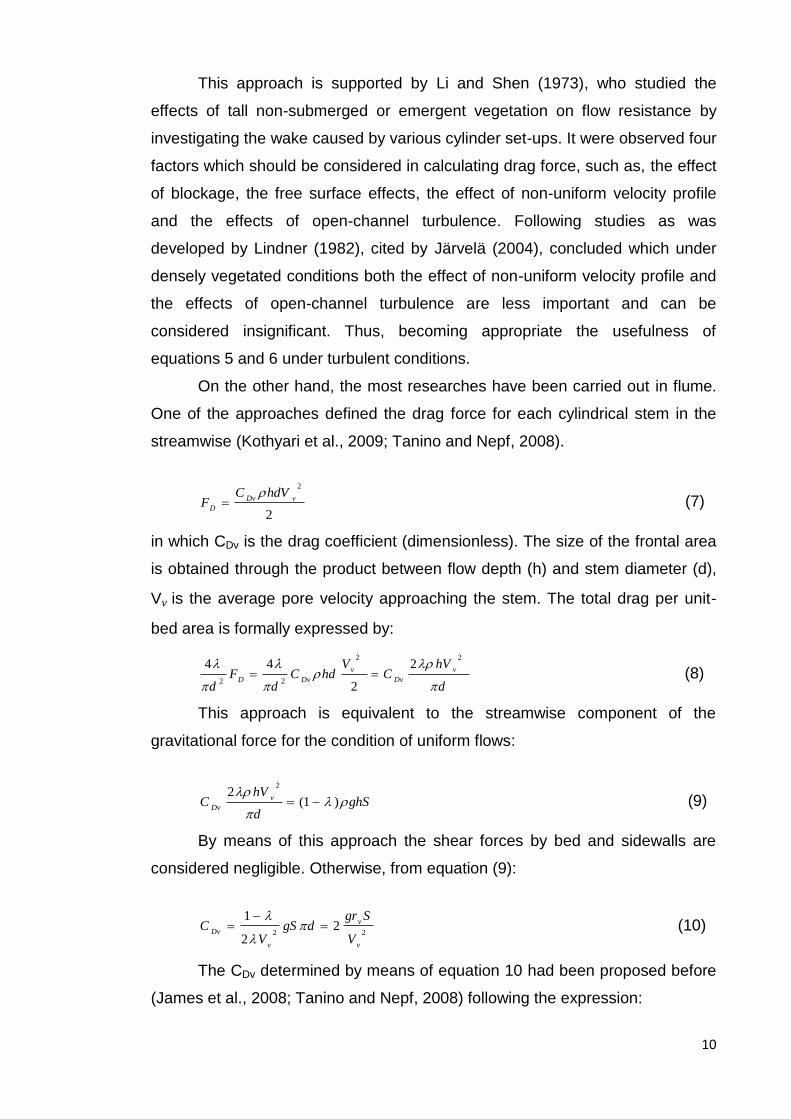
The vegetation drag coefficient can be expressed by assuming that the

gravitational force is equal to the drag of vegetation and the friction at the

streambed of the channel is negligible in the presence of vegetation (Wu et al.,

1999):

2

2'

V

gSC

D (5)

in which CD’ is the vegetation drag coefficient (m-1), g is the gravitational

acceleration (m s-2), S is the slope of the channel bottom (m m-1), V is the mean

flow velocity (m s-1), and “ ” is the ratio between h and y, flow depth (m) and

vegetation thickness (m), respectively. For unsubmerged vegetation, α equals

1.

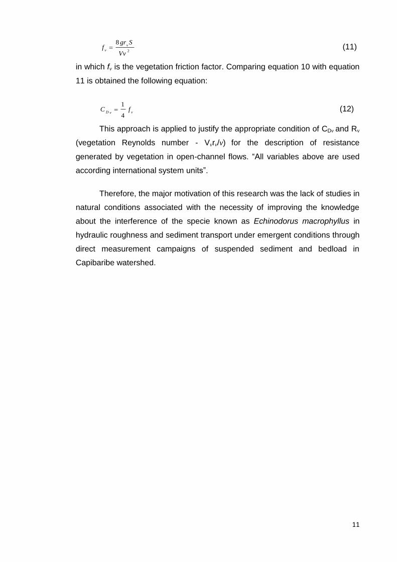
Expanding the description of vegetation resistance force previously

introduced by several authors (Kao et al., 1977; Maheshwari, 1992), Lee et al.

(2004) considered in their experiment flow through a vertical segment, with

plants in multiple spatial arrangements, and found the total vegetation

resistance force as:

2

2VaC

F D

D

(6)

in which: FD is the vegetation resistance force (N m-3), a is the total projected

plant area per unit volume (m2 m-3) given the diameter of the Echinodorus

macrophyllus leaves, ρ is the density of water (kg m-3). To make CD’

dimensionless, it must be multiplied by an equivalent flow width.

10

This approach is supported by Li and Shen (1973), who studied the

effects of tall non-submerged or emergent vegetation on flow resistance by

investigating the wake caused by various cylinder set-ups. It were observed four

factors which should be considered in calculating drag force, such as, the effect

of blockage, the free surface effects, the effect of non-uniform velocity profile

and the effects of open-channel turbulence. Following studies as was

developed by Lindner (1982), cited by Järvelä (2004), concluded which under

densely vegetated conditions both the effect of non-uniform velocity profile and

the effects of open-channel turbulence are less important and can be

considered insignificant. Thus, becoming appropriate the usefulness of

equations 5 and 6 under turbulent conditions.

On the other hand, the most researches have been carried out in flume.

One of the approaches defined the drag force for each cylindrical stem in the

streamwise (Kothyari et al., 2009; Tanino and Nepf, 2008).

2

2

vDv

D

hdVCF

(7)

in which CDv is the drag coefficient (dimensionless). The size of the frontal area

is obtained through the product between flow depth (h) and stem diameter (d),

Vv is the average pore velocity approaching the stem. The total drag per unit-

bed area is formally expressed by:

d

hVC

VhdC

dF

d

v

Dv

v

DvD

22

22

2

2

44 (8)

This approach is equivalent to the streamwise component of the

gravitational force for the condition of uniform flows:

ghSd

hVC v

Dv

)1(

22

(9)

By means of this approach the shear forces by bed and sidewalls are

considered negligible. Otherwise, from equation (9):

222

2

1

v

v

v

Dv

V

SgrdgS

VC

(10)

The CDv determined by means of equation 10 had been proposed before

(James et al., 2008; Tanino and Nepf, 2008) following the expression:

11

2

8

Vv

Sgrf

v

v (11)

in which fv is the vegetation friction factor. Comparing equation 10 with equation

11 is obtained the following equation:

vvDfC

4

1 (12)

This approach is applied to justify the appropriate condition of CDv and Rv

(vegetation Reynolds number - Vvrv/v) for the description of resistance

generated by vegetation in open-channel flows. “All variables above are used

according international system units”.

Therefore, the major motivation of this research was the lack of studies in

natural conditions associated with the necessity of improving the knowledge

about the interference of the specie known as Echinodorus macrophyllus in

hydraulic roughness and sediment transport under emergent conditions through

direct measurement campaigns of suspended sediment and bedload in

Capibaribe watershed.

12

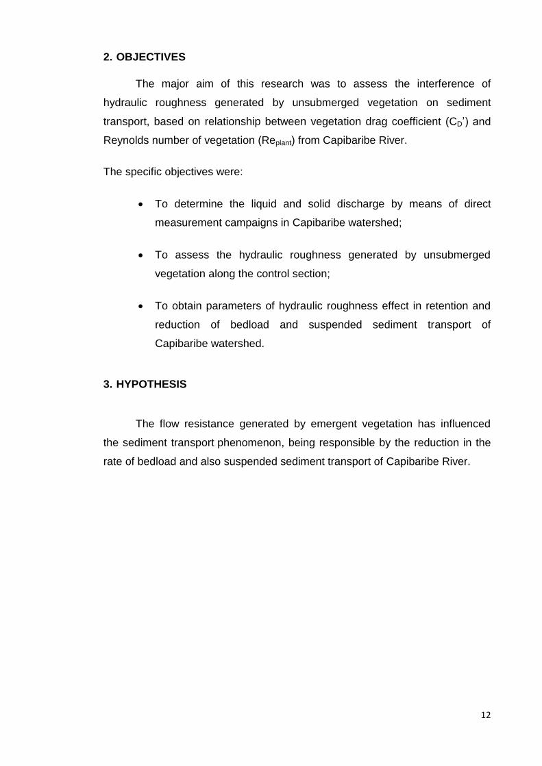
2. OBJECTIVES

The major aim of this research was to assess the interference of

hydraulic roughness generated by unsubmerged vegetation on sediment

transport, based on relationship between vegetation drag coefficient (CD’) and

Reynolds number of vegetation (Replant) from Capibaribe River.

The specific objectives were:

To determine the liquid and solid discharge by means of direct

measurement campaigns in Capibaribe watershed;

To assess the hydraulic roughness generated by unsubmerged

vegetation along the control section;

To obtain parameters of hydraulic roughness effect in retention and

reduction of bedload and suspended sediment transport of

Capibaribe watershed.

3. HYPOTHESIS

The flow resistance generated by emergent vegetation has influenced

the sediment transport phenomenon, being responsible by the reduction in the

rate of bedload and also suspended sediment transport of Capibaribe River.

13

4. MATERIALS AND METHODS

4.1. Study area description

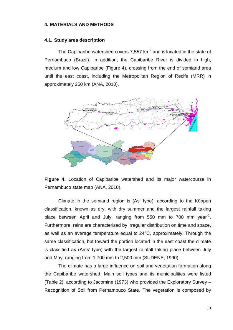
The Capibaribe watershed covers 7,557 km2 and is located in the state of

Pernambuco (Brazil). In addition, the Capibaribe River is divided in high,

medium and low Capibaribe (Figure 4), crossing from the end of semiarid area

until the east coast, including the Metropolitan Region of Recife (MRR) in

approximately 250 km (ANA, 2010).

Figure 4. Location of Capibaribe watershed and its major watercourse in

Pernambuco state map (ANA, 2010).

Climate in the semiarid region is (As’ type), according to the Köppen

classification, known as dry, with dry summer and the largest rainfall taking

place between April and July, ranging from 550 mm to 700 mm year-1.

Furthermore, rains are characterized by irregular distribution on time and space,

as well as an average temperature equal to 24°C, approximately. Through the

same classification, but toward the portion located in the east coast the climate

is classified as (Ams’ type) with the largest rainfall taking place between July

and May, ranging from 1,700 mm to 2,500 mm (SUDENE, 1990).

The climate has a large influence on soil and vegetation formation along

the Capibaribe watershed. Main soil types and its municipalities were listed

(Table 2), according to Jacomine (1973) who provided the Exploratory Survey –

Recognition of Soil from Pernambuco State. The vegetation is composed by

14

shrubs (caatinga) in semiarid portion and partially covered by sugar cane and

pasture in the eastern part of the watershed (ANA, 2010).

Table 2. Predominance of some classes of soils in Capibaribe watershed

(USDA, 1999).

Watershed Relevant Predominant

division Municipalities Soils

Santa Cruz do Capibaribe;

High Brejo da Madre de Deus; Oxisols; Ultisols

Capibaribe Belo Jardim; Pesqueira; Poção; Albaquults; Vertisols;

Taquaritinga do Norte; Brejo Alfisols and Entisols.

da Madre de Deus and so on.

Caruaru; Limoeiro; Gravatá;

Middle Salgadinho; Toritama; Bezerros; Entisols; Albaquults;

Capibaribe Limoeiro; Feira Nova; Frei Vertisols and Inceptisols.

Miguelino and so on.

Paudalho; Glória de Goitá;

Low Pombos; São Lourenço da Mata;

Capibaribe Tracunhaém; Vitória de Santo Oxisols; Ultisols and

Antão; Camaragibe; Recife and Entisols (Aqu-alf-and-

so on. ent-ept-)

4.2. Physical-hydric characteristics of Capibaribe Watershed

The physical-hydric characteristics of Capibaribe watershed and its

hydrological response can be found in (Table 3). The form coefficient was

determined following the equation proposed by (Ponce, 1989).

2L

AKf (13)

in which Kf is the form coefficient (dimensionless), A is the watershed area

(km2), L is the length of the main watercourse (km).

The water line slope was calculated according to Simons and Senturk, (1997):

D

gVVhhS

upstreamdownstreamupstreamdownstream

w

2/)()(2222

(14)

15

in which Sw is the water line slope (m m-1); h is the flow depth (m); V is the

average flow velocity (m s-1), g is the gravitational acceleration (m s-2) and D is

the distance between crosses sections.

Table 3. Physical-hydric characteristics of the Capibaribe watershed.

Characteristics Values

Area 7,557 Km2

Main lenght 250 Km

Form coefficient 0.12 (dim.)

Maximum elevation 1,200 m

Minimum elevation 2.0 m

Watershed slope 0.039 m m-1

Water surface slope 0.0076 m m-1

Concentration time 30 h

4.3. Crosses sections and direct measurement campaigns

This research was performed by means of thirteen direct measurement

campaigns of water discharge and solid discharge during 2011 year, evaluating

different conditions, such as, the effects of presence and absence of emergent

vegetation on sediment transport phenomenon. Thereby, during four months

(January, February, March and April) were carried out eight campaigns for

making a comparison between nonvegetated and vegetated crosses sections,

both with the same water surface slope. The remainder campaigns were carried

out in a cross section without vegetation due to the high level of water discharge

which provides the removal of aquatic specie.

The crosses sections were located in a community known as Mussurepe,

located in Paudalho – PE, 35°05’23.6’’ W e 07°55’06’’ S (Figure 5). First of all,

it was essential to choose adequate crosses sections before carrying out the

direct measurements campaigns. Therefore, both were situated on a flat stretch

and free from effects that could cause disturbances in the flow, such as

backwater effects; well-defined banks and no flow reduction downstream.

16

Figure 5. Location of crosses sections in Capibaribe River.

In addition, the crosses sections were chosen far from watershed outlet

aiming to narrow down or eliminate the effect of tidal advection on sediment

transport measurements (Araújo et al., 2008).

4.4. Velocity measurement

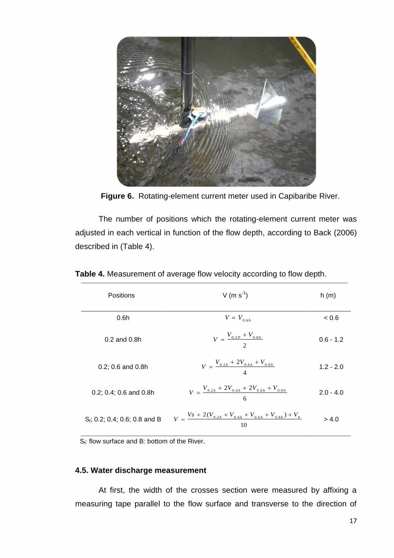
During the campaigns in Capibaribe River the flow velocity was

determined by rotating current meter (Figure 6), which is based on the

proportionality between the angular velocity of the rotation device and the flow

velocity. In others words, the flow velocity was acquired by counting the number

of revolutions of the propeller in a measured time interval, which was thirty

seconds for all campaigns. The depth-average velocity was obtained in the

cross section through a measurement velocity profile. In some campaigns,

mainly during low water discharges was used the Hidromec mini model due to

low flow depth.

17

Figure 6. Rotating-element current meter used in Capibaribe River.

The number of positions which the rotating-element current meter was

adjusted in each vertical in function of the flow depth, according to Back (2006)

described in (Table 4).

Table 4. Measurement of average flow velocity according to flow depth.

Positions V (m s-1

) h (m)

0.6h hVV

6.0 < 0.6

0.2 and 0.8h 2

8.02.0 hPVV

V

0.6 - 1.2

0.2; 0.6 and 0.8h 4

28.06.02.0 hhh

VVVV

1.2 - 2.0

0.2; 0.4; 0.6 and 0.8h 6

228.06.04.02.0 hhhh

VVVVV

2.0 - 4.0

Sf; 0.2; 0.4; 0.6; 0.8 and B 10

)(28.06.04.02.0 bhhhh

VVVVVVsV

> 4.0

Sf: flow surface and B: bottom of the River.

4.5. Water discharge measurement

At first, the width of the crosses section were measured by affixing a

measuring tape parallel to the flow surface and transverse to the direction of

18

flow from the left bank of the stream to the right bank and the flow depth of each

vertical was obtained by specific measuring rule. The crosses sections were

divided into a series of vertical lines with the same width, varying according to

the total width of the water flow at the moment of measuring, according to the

equal-width-increment (EWI), method proposed by Edwards and Glysson

(1999).

The crosses sections areas were determined obtaining the area of each

vertical through the assumption which the first and last segments can be

consider a triangular shape and others as trapezium. Therefore, the total area

of each cross section was acquired by the sum of all vertical.

The water discharge was determined by computing the product of the

mean flow velocity (m s-1) and the area of influence (m2) for each segment in

the section and then summing these products over all segments (Equation 15).

iii

VAQQ (15)

in which Q is the water discharge (m3 s-1), Qi is the water discharge in each

vertical segment (m3 s-1), Ai is the influence area of the vertical segment (m2),

and Vi is the average flow velocity in the influence area of each vertical segment

(m s-1).

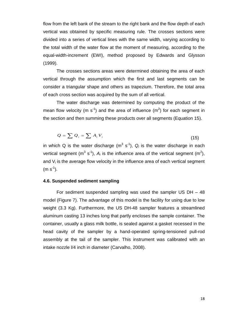
4.6. Suspended sediment sampling

For sediment suspended sampling was used the sampler US DH – 48

model (Figure 7). The advantage of this model is the facility for using due to low

weight (3.3 Kg). Furthermore, the US DH-48 sampler features a streamlined

aluminum casting 13 inches long that partly encloses the sample container. The

container, usually a glass milk bottle, is sealed against a gasket recessed in the

head cavity of the sampler by a hand-operated spring-tensioned pull-rod

assembly at the tail of the sampler. This instrument was calibrated with an

intake nozzle l/4 inch in diameter (Carvalho, 2008).

19

Figure 7. Suspended sediment sampling (sampler - US DH-48) in Capibaribe

River.

The methodology used to the measurements of suspended sediment

concentration (SSC) was EWI (Figure 8), which is a specific method indicated

for resulting in the collection of discharge-weighted, depth-integrated, isokinetic

samples, proposed by Edwards and Glysson (1999). The basic approach of this

method is which a cross section is divided in equally spaced segments and the

sampler is carried out in the middle part of each segment. Moreover, during the

sampling the descending and ascending transit rate must be the same along

the traverse of each vertical, resulting in a volume of water proportional to the

flow in each vertical (Edwards and Glysson, 1999).

20

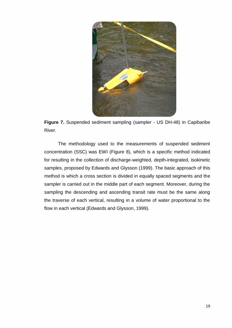
Figure 8. Equal-width-increment vertical transit rate relative to sample volume,

which is proportional to water discharge at each vertical.

The transit rate depend on several features, such as, sample volume

collected, size of the nozzle in sampling equipment, depth of the sample taken

and flow velocity (Wilde and Radtke, 1998). Thereby, according to USGS

(2005) the transit rate was expressed as:

KVVti

__

(16)

in which Vt is the transit rate (m s-1), and K is the constant of variable

proportionality according to each different nozzle used, which was 0.4 for the ¼”

nozzle of the sampler. Nevertheless, the information used during sampling was

not the transit rate, but the time for the sampler to descend to the streambed

and return to the water surface, calculated by the expression proposed by

Carvalho et al. (2000); Merten and Poleto (2006).

Vt

ht

21 (17)

in which t1 represents the minimum time of the suspended sediment sampling

(s). A small distance was subtracted from the value of h to account for the fact

that the equipment would not contact the streambed (10 or 15 cm).

All collected samples in each segment (vertical) of the crosses sections

in Capibaribe River were individually preserved to determine the SSC in Soil

Conservation Engineering Laboratory at UFRPE, which was determined

through the ratio between the suspended sediment mass and liquid volume of

the sample, according to evaporation method (USGS, 1973).

21

sampleVol

MSSC (18)

in which SSC is the suspended sediment concentration in the sampled vertical

(mg L-1), M is the suspended sediment mass (mg) and Volsample is the sample

volume (L). For checking the accuracy of suspended sediment sampling was

calculated the Box coefficient (BC), following the proposed by USGS (2005).

iSSC

SSCBC

_____

(19)

in which BC is the Box Coefficient (dimensionless), SSC is the average of

suspended sediments concentration (mg L-1) and SSCi is the suspended

sediment concentration at each vertical (mg L-1).

After obtaining the Q and SSCi in each vertical was acquired the

suspended solid discharge (SSQ), which represents the amount of suspended

sediment crossing the cross section per day, in the form of an expression found

in Horowitz (2003).

0864.0)( QSSCSSQi

(20)

in which SSQ is the suspended solid discharge (t day-1) and 0.0864 is a

constant for unit adjustment.

4.7. Bedload discharge and particle size distribution

The bedload discharge was determined in each campaign by means of a

bedload sampler US BLH – 84 model (Figure 9), which was projected for

collecting sediments ranging from 1 to 38 mm (Diplas et al., 2008).

22

Figures 9. Bedload sampling with the sampler US BLH – 84 model.

After sampling, the bedload discharge was calculated according to Gray

(2005):

0864.0

2

xL

wt

mQB

(21)

in which QB is bedload discharge (t day-1), m is the mass of sediment from

bedload transport in each vertical (g), w is the width of nozzle which is

considered 0.075 m, t2 is the sampling time of bedload transport (30 s), Lx is the

equivalent width (m).

Understanding regarding particle size distribution is fundamental for

several quantitative and qualitative purposes. This sort of study can be useful

for providing information about the source and travel distance of sediment, as

well as predict channel form and stability (Bunte and Abt, 2001).

The total bedload mass of each campaign was dried in oven (65 °C).

Afterward, it was used to obtain the particle size distribution. The process

consists in sieving each sample in a electromagnetic shaker, Viatest VSM 200

model (Figure 10) equipped with a group of sieves in decrease diameters order

(3.35; 1.7; 0.85; 0.60; 0.425; 0.30; 0.212; 0.150; 0.20; 0.106; 0.076 e 0.053

mm), during 10 minutes under 90 vibrations per second. As a result, it was

possible to obtain the particle size distribution curve and also calculate the

median grain diameter (d50) through the Curve Expert 1.3 (2005) programmer.

23

Figure 10. Test sieve shaker used to determine the particle size distribution.

4.8. Hydraulic characteristics and vegetation resistance parameters

To measure the wetted perimeter was necessary to divide the crosses

sections into vertical segments of equal width, as well done to the area and

other variables calculated in the project. Then, it was obtained the hydraulic

radius, which was calculated by the ratio of cross-section area to wetted

perimeter.

Reynolds and Froud numbers relate the inertia forces to the viscous

forces usually involved wherever viscosity is fundamental as in slow movement

of fluid in small passages or around small objects and with the gravitational

effects considered important wherever the gravity effect is dominant,

respectively. These variables are formally expressed according to Simons and

Sentürk (1992).

v

VRh

Re (22)

hgR

VFr (23)

in which Re is the Reynolds number (dimensionless), Fr is the Froud number

(dimensionless) and Rh is the hydraulic radius (m).

24

The kinematic viscosity of water was estimated using the equation

proposed by Julien (1995).

6210])15(00068.0)15(031.014.1[

TTv (24)

in which v is kinematic viscosity of water (m2 s-1) and T is the temperature of

water in degrees Celsius. The plant Reynolds number was calculated using an

approximation proposed by Lee et al. (2004):

v

Vsplant

Re (25)

in which Replant is dependent on vegetation type (dimensionless), s is the

spacing between plants (m).

The vegetation drag force was calculated using the Equation 6, as

proposed by Lee et al. (2004) and the plant drag coefficient was obtained

applying Equation 5, according to Wu et al. (1999).

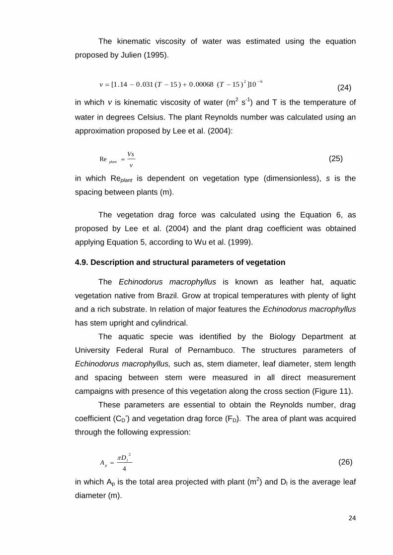
4.9. Description and structural parameters of vegetation

The Echinodorus macrophyllus is known as leather hat, aquatic

vegetation native from Brazil. Grow at tropical temperatures with plenty of light

and a rich substrate. In relation of major features the Echinodorus macrophyllus

has stem upright and cylindrical.

The aquatic specie was identified by the Biology Department at

University Federal Rural of Pernambuco. The structures parameters of

Echinodorus macrophyllus, such as, stem diameter, leaf diameter, stem length

and spacing between stem were measured in all direct measurement

campaigns with presence of this vegetation along the cross section (Figure 11).

These parameters are essential to obtain the Reynolds number, drag

coefficient (CD’) and vegetation drag force (FD). The area of plant was acquired

through the following expression:

4

2

l

p

DA

(26)

in which Ap is the total area projected with plant (m2) and Dl is the average leaf

diameter (m).

25

Figure 11. Measurement of vegetation structural parameters.

In brief, the characteristic of stem upright is far too important for

considering negligible the flexible effects of this specie, evaluated under

emergent conditions, which is fundamental to provide an adequate assessment

of vegetation drag coefficient and vegetation drag force.

4.10. Statistical analysis

Principal component analysis (PCA) and hierarchical cluster analysis

(HCA) were performed through the STATISTICA 7 software, considering the

sediment transport of thirteen direct measurement campaigns carried out in

Capibaribe River along 2011. The regression analysis was used to analyze the

relationship between some parameters, such as, flow depth, water discharge,

suspended sediment concentration, vegetation drag force, vegetation drag

coefficient and vegetation Reynolds number.

5. RESULTS AND DISCUSSION

5.1. Rainfall in Capibaribe River

The average rainfall for the rainy and dry seasons of the years

2010 and 2011, as well as the historical average monthly are shown in Figure

12. The highest rainfall was observed for the direct measurement campaign

26

carried out in Capibaribe River in May with a value equal to 574 mm, exceeding

the historical average for this month.

Figure 12. Distribution of average annual rainfall for non-rainy and rainy 2010

and 2011, as well as the historical average in Capibaribe River (LAMEPE,

2011).

5.2. Hydraulic characteristics and rating curve of Capibaribe River

The hydraulic radius ranged from 0.51 m for a shear stress (τ) equal to

37.87 N m-2 until 0.82 m for a τ equal to 61.35 N m-2. Moreover, the highest τ

equal to 61.35 was responsible by the highest value of bedload transport equal

to 5.82 t day-1 (Table 5).

Combined effect of viscosity and gravity provided the regime of flow in

Capibaribe watershed, which was classified as turbulent subcritical due to the

Reynolds numbers greater than 2500, and Froud numbers less than a unity

(Simons and Sentürk, 1992). As a result, the viscous forces are weak in

comparison with the inertial forces and the fluid particles move in irregular

paths. The median grain diameter (d50) predominantly showed a great

uniformity of the particles transported in the stream bed with a standard

deviation equal to 0.05 (Table 5), except for the direct measurement campaign

performed in August.

0

150

300

450

600

Jan Feb Mar Apr May Jun Jul Agu Sep Oct

Rain

fall

(m

m)

Months

2010

2011

Historical

27

Table 5. Hydraulic variables of direct measurements campaigns performed

under nonvegetated conditions in Capibaribe River.

Campaigns Rh Re Fr τ d50 Texture

m -------dim.------- N m-2 mm

25/1/2011 0.60 238382.88 0.15 44.65 0.51 coarse sand

3/2/2011 0.51 205453.60 0.15 37.87 0.53 coarse sand

18/3/2011 0.52 247756.83 0.18 38.54 0.49 medium sand

13/4/2011 0.66 444072.41 0.23 49.36 0.51 coarse sand

29/5/2011 0.71 294539.20 0.13 53.18 0.64 coarse sand

26/8/2011 0.82 163084.61 0.06 61.35 0.61 coarse sand

14/9/2011 0.79 142632.13 0.06 58.93 0.52 coarse sand

6/10/2011 0.76 201543.25 0.08 56.93 0.27 fine sand

13/10/2011 0.73 156385.58 0.07 54.72 0.56 coarse sand

Mean 0.68 232650.05 0.12 50.61 0.52

Rh: hydraulic radius; Re: Reynolds number; Fr: Froude number; τ: shear stress; d50: median

grain diameter.

In Figure 13 it was observed the particle size distribution curve of the

direct measurement campaign carried out in 29/05/2011 with the d50 equal to

0.64 mm.

Figure 13. Particle size distribution curve of sediment transported in the

streambed by Capibaribe River in 29/05/2011.

The rating curve relating water discharge (Q) and flow depth (h) provided

a determination coefficient equal to 0.74, considering the direct measurement

campaigns carried out without vegetation along the crosses sections and Q

S = 1.24668873

r = 0.99960332

Diameter of sieves (m)

Su

m o

f c

las

ses

(%

)

0.0 0.6 1.2 1.8 2.5 3.1 3.70.00

18.33

36.67

55.00

73.33

91.67

110.00

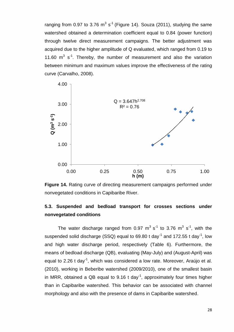
28

ranging from 0.97 to 3.76 m3 s-1 (Figure 14). Souza (2011), studying the same

watershed obtained a determination coefficient equal to 0.84 (power function)

through twelve direct measurement campaigns. The better adjustment was

acquired due to the higher amplitude of Q evaluated, which ranged from 0.19 to

11.60 m3 s-1. Thereby, the number of measurement and also the variation

between minimum and maximum values improve the effectiveness of the rating

curve (Carvalho, 2008).

Figure 14. Rating curve of directing measurement campaigns performed under

nonvegetated conditions in Capibaribe River.

5.3. Suspended and bedload transport for crosses sections under

nonvegetated conditions

The water discharge ranged from 0.97 m3 s-1 to 3.76 m3 s-1, with the

suspended solid discharge (SSQ) equal to 69.80 t day-1 and 172.55 t day-1, low

and high water discharge period, respectively (Table 6). Furthermore, the

means of bedload discharge (QB), evaluating (May-July) and (August-April) was

equal to 2.26 t day-1, which was considered a low rate. Moreover, Araújo et al.

(2010), working in Beberibe watershed (2009/2010), one of the smallest basin

in MRR, obtained a QB equal to 9.16 t day-1, approximately four times higher

than in Capibaribe watershed. This behavior can be associated with channel

morphology and also with the presence of dams in Capibaribe watershed.

Q = 3.647h2.708

R² = 0.76

0.00

1.00

2.00

3.00

4.00

0.00 0.25 0.50 0.75 1.00

Q (

m3

s-1

)

h (m)

29

Table 6. Sediment transport variables of directing measurement campaigns

performed in the crosses sections under nonvegetated conditions.

Campaigns Q SSQ

QB (QB/SSQ)

x100 BC

m3 s-1 ------t day-1------ (%) ----dim.----

25/1/2011 1.43 89.32 0.19 0.21 0.86-1.13

3/2/2011 0.97 69.80 0.18 0.26 0.86-1.40

18/3/2011 1.01 75.78 0.14 0.18 0.93-1.25

13/4/2011 2.20 153.77 0.57 0.37 0.83-1.18

29/5/2011 3.76 172.55 2.14 1.24 0.74-1.36

26/8/2011 2.64 166.08 5.82 3.51 0.66-1.13

14/9/2011 2.56 172.41 2.97 1.72 0.85-1.08

6/10/2011 2.62 206.12 5.32 2.58 1.05-1.26

13/10/2011 2.75 224.84 3.85 1.71 0.86-1.12

Mean 2.22 147.85 2.26 1.31 ------ Q: water discharge; SSQ: suspended solid discharge; QB: bedload discharge and BC: box

coefficient.

The ratio between QB and SSQ ranged from 0.18% to 3.51% with the

mean value equal to 1.31% (Table 6). Usually, the bedload transport rate of a

River is about 5-25% of the suspended sediment transport (Yang, 1996).

Nevertheless, the low rates can be attributed to the presence of dams which

have been admitted to have a strong effect on sediment transport as was

discussed by Preciso et al. (2011) which evidenced the reduction on sediment

supply at River Reno, but without quantifying this process due to the lack of

assessment before dam construction. In addition, the values of individual

suspended sediment samples showed adequate box coefficient (BC), ranging

from 0.9 to 1.2 or within the acceptable limits, ranging from 0.67 to 1.5 (Gray,

2005).

The relation between suspended sediment concentration (SSC) and Q

was expressing by a rating curve (Figure 15). It was observed which the SSC

was not influenced directly by the Q due to the low determination coefficient

equal to 0.21, demonstrating the large complexity and variability associated with

the SSC measurements. Furthermore, this behavior represents the effects of

dams, as was discussed by Baker et al. (2011) which evaluated the

downstream effects of dams, mainly in suspended sediment. In the same way,

Souza (2011) working in the Capibaribe watershed obtained low adjustment

between SSC and Q discharge (R2 equal to 0.14). Moreover, the high variability

30

between SSC and Q was emphasized by Saeidi et al. (2011) which obtained a

high variability of regression coefficients.

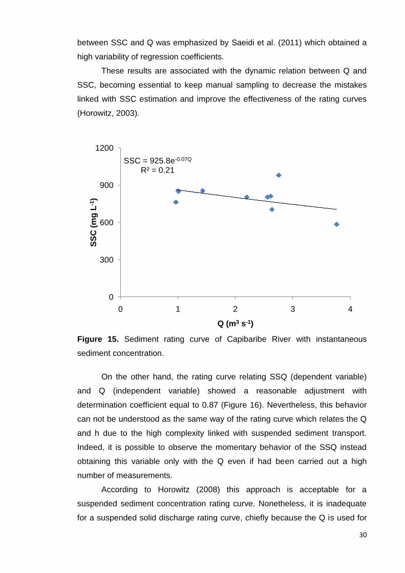
These results are associated with the dynamic relation between Q and

SSC, becoming essential to keep manual sampling to decrease the mistakes

linked with SSC estimation and improve the effectiveness of the rating curves

(Horowitz, 2003).

Figure 15. Sediment rating curve of Capibaribe River with instantaneous

sediment concentration.

On the other hand, the rating curve relating SSQ (dependent variable)

and Q (independent variable) showed a reasonable adjustment with

determination coefficient equal to 0.87 (Figure 16). Nevertheless, this behavior

can not be understood as the same way of the rating curve which relates the Q

and h due to the high complexity linked with suspended sediment transport.

Indeed, it is possible to observe the momentary behavior of the SSQ instead

obtaining this variable only with the Q even if had been carried out a high

number of measurements.

According to Horowitz (2008) this approach is acceptable for a

suspended sediment concentration rating curve. Nonetheless, it is inadequate

for a suspended solid discharge rating curve, chiefly because the Q is used for

SSC = 925.8e-0.07Q

R² = 0.21

0

300

600

900

1200

0 1 2 3 4

SS

C (

mg

L-1

)

Q (m3 s-1)

31

obtaining the SSQ. Accordingly, it is common to observe the increase in

determination coefficient, but without increasing the importance of the rating

curve relating Q and SSQ.

Figure 16. Suspended sediment rating curve of Capibaribe watershed.

5.4. Interference of unsubmerged vegetation on sediment transport of

Capibaribe watershed

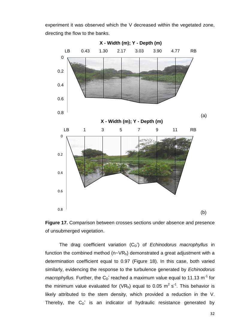
The Figures 17a and 17b represent the crosses sections evaluated in

03/02/2011, under nonvegetated and vegetated conditions, respectively. The h

was more uniform in the cross section 17a. The vegetated zone in cross section

(Figure 17b) leaded an increase equal to 24% in the average flow velocity at

nonvegetated zone. Likely, the vegetated zone decreased the h due to an

increase on sediment deposition.

According to Cheng (2008) the decrease in sediment transport capacity

and an increased in sedimentation is influenced by the momentum losses

generated by vegetation. Further, this tendency was highlighted by Bennett et

al. (2002), which conducted an experiment with simulated emergent stiff

vegetation using several densities in laboratory flume channel. In this

SSQ = 74.62Q0.860

R² = 0.87

0.0

75.0

150.0

225.0

300.0

0.0 1.0 2.0 3.0 4.0

SS

Q (

t d

ay

-1)

Q (m3 s-1)

32

experiment it was observed which the V decreased within the vegetated zone,

directing the flow to the banks.

(a)

(b)

Figure 17. Comparison between crosses sections under absence and presence

of unsubmerged vegetation.

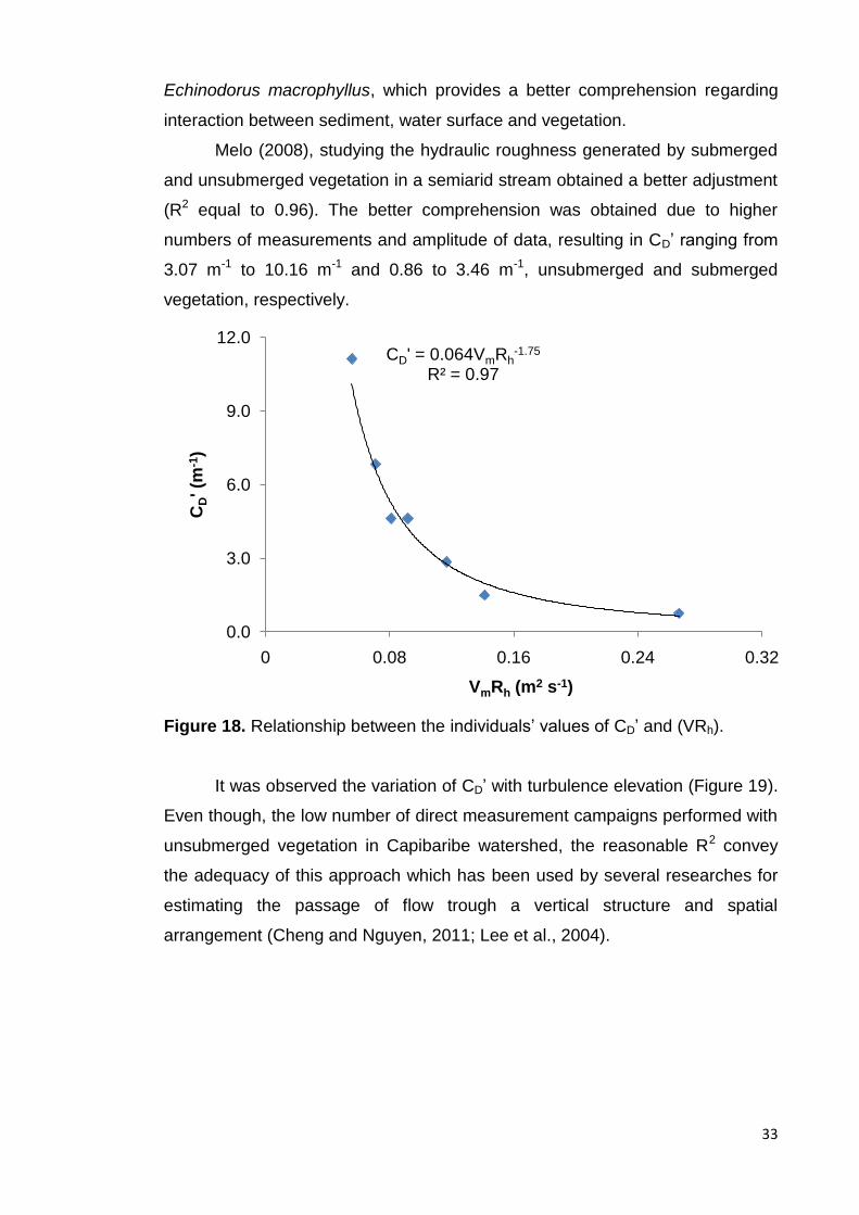
The drag coefficient variation (CD’) of Echinodorus macrophyllus in

function the combined method (n~VRh) demonstrated a great adjustment with a

determination coefficient equal to 0.97 (Figure 18). In this case, both varied

similarly, evidencing the response to the turbulence generated by Echinodorus

macrophyllus. Further, the CD’ reached a maximum value equal to 11.13 m-1 for

the minimum value evaluated for (VRh) equal to 0.05 m2 s-1. This behavior is

likely attributed to the stem density, which provided a reduction in the V.

Thereby, the CD’ is an indicator of hydraulic resistance generated by

0

0.2

0.4

0.6

0.8

LB 0.43 1.30 2.17 3.03 3.90 4.77 RB

0

0.2

0.4

0.6

0.8

LB 1 3 5 7 9 11 RB

X - Width (m); Y - Depth (m)

X - Width (m); Y - Depth (m)

33

Echinodorus macrophyllus, which provides a better comprehension regarding

interaction between sediment, water surface and vegetation.

Melo (2008), studying the hydraulic roughness generated by submerged

and unsubmerged vegetation in a semiarid stream obtained a better adjustment

(R2 equal to 0.96). The better comprehension was obtained due to higher

numbers of measurements and amplitude of data, resulting in CD’ ranging from

3.07 m-1 to 10.16 m-1 and 0.86 to 3.46 m-1, unsubmerged and submerged

vegetation, respectively.

Figure 18. Relationship between the individuals’ values of CD’ and (VRh).

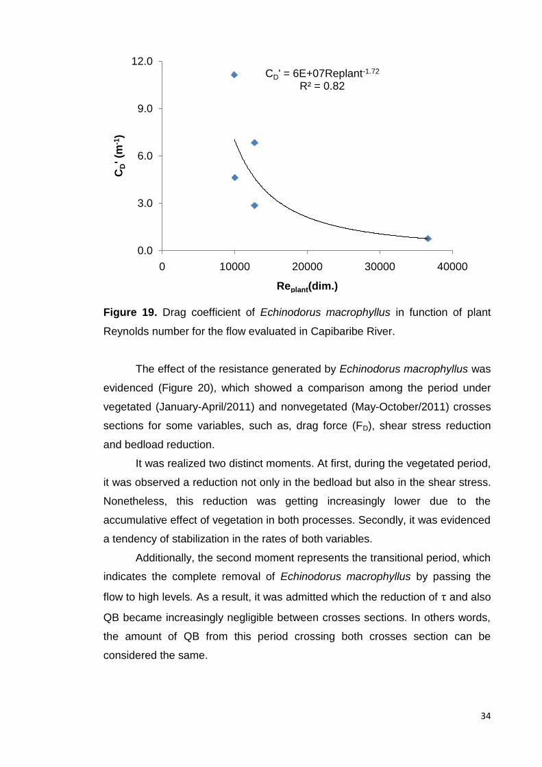
It was observed the variation of CD’ with turbulence elevation (Figure 19).

Even though, the low number of direct measurement campaigns performed with

unsubmerged vegetation in Capibaribe watershed, the reasonable R2 convey

the adequacy of this approach which has been used by several researches for

estimating the passage of flow trough a vertical structure and spatial

arrangement (Cheng and Nguyen, 2011; Lee et al., 2004).

CD' = 0.064VmRh-1.75

R² = 0.97

0.0

3.0

6.0

9.0

12.0

0 0.08 0.16 0.24 0.32

CD' (m

-1)

VmRh (m2 s-1)

34

Figure 19. Drag coefficient of Echinodorus macrophyllus in function of plant

Reynolds number for the flow evaluated in Capibaribe River.

The effect of the resistance generated by Echinodorus macrophyllus was

evidenced (Figure 20), which showed a comparison among the period under

vegetated (January-April/2011) and nonvegetated (May-October/2011) crosses

sections for some variables, such as, drag force (FD), shear stress reduction

and bedload reduction.

It was realized two distinct moments. At first, during the vegetated period,

it was observed a reduction not only in the bedload but also in the shear stress.

Nonetheless, this reduction was getting increasingly lower due to the

accumulative effect of vegetation in both processes. Secondly, it was evidenced

a tendency of stabilization in the rates of both variables.

Additionally, the second moment represents the transitional period, which

indicates the complete removal of Echinodorus macrophyllus by passing the

flow to high levels. As a result, it was admitted which the reduction of τ and also

QB became increasingly negligible between crosses sections. In others words,

the amount of QB from this period crossing both crosses section can be

considered the same.

CD' = 6E+07Replant-1.72

R² = 0.82

0.0

3.0

6.0

9.0

12.0

0 10000 20000 30000 40000

CD' (m

-1)

Replant(dim.)

35

Figure 20. Relationship between drag force, shear stress reduction and

bedload reduction during vegetated and unvegetated period.

5.5. Multivariate analysis

The multivariate analysis was carried out to become the discussion more

practical. Therefore, it was applied principal components analysis (PCA) for

selecting the major variables associated with the sediment transport in

Capibaribe watershed. Afterward, the hierarchical cluster analysis (HCA) was

performed to attempt distinguish the effect of flow resistance generated by

Echinodorus macrophyllus on sediment transport phenomenon.

5.6. Principal component analysis

The principal component analysis was applied to the sixteen variables to

select the most important variables for explaining the sediment transport and

the effect of unsubmerged vegetation on sediment transport rate. The selection

of variables was based exclusively in sequential tests for analyzing the

contribution of each one.

Principal components were extracted through the correlation matrix

computed for the eleven variables previously selected. The first two

components extracted had eigenvalues equal to 6.74 and 3.15, accounting for

the 90.03% of the total variance explained (Table 7). Furthermore, only the first

two components were used because presented eigenvalues greater than 1 as

0.00

0.05

0.10

0.15

0.20

0.0

2.5

5.0

7.5

10.0

Jan Fev Mar Apr May Ago Sep Oct Oct

Bed

load

re

du

cti

on

(t

da

y-1

)

FD

(N m

-3)

an

d s

hea

r s

tres

s

red

ucti

on

(N

m-2

)

Shear stress reduction F Bedload reduction

Vegetated Nonvegetated

D

Feb Aug

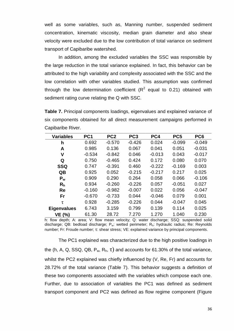
36

well as some variables, such as, Manning number, suspended sediment

concentration, kinematic viscosity, median grain diameter and also shear

velocity were excluded due to the low contribution of total variance on sediment

transport of Capibaribe watershed.

In addition, among the excluded variables the SSC was responsible by

the large reduction in the total variance explained. In fact, this behavior can be

attributed to the high variability and complexity associated with the SSC and the

low correlation with other variables studied. This assumption was confirmed

through the low determination coefficient (R2 equal to 0.21) obtained with

sediment rating curve relating the Q with SSC.

Table 7. Principal components loadings, eigenvalues and explained variance of

six components obtained for all direct measurement campaigns performed in

Capibaribe River.

Variables PC1 PC2 PC3 PC4 PC5 PC6

h 0.692 -0.570 -0.426 0.024 -0.099 -0.049

A 0.985 0.136 0.067 0.041 0.051 -0.031

V -0.534 -0.842 0.046 -0.013 0.043 -0.017

Q 0.750 -0.465 0.424 0.172 0.080 0.070

SSQ 0.747 -0.391 0.460 -0.222 -0.169 0.003

QB 0.925 0.052 -0.215 -0.217 0.217 0.025

Pw 0.909 0.290 0.264 0.058 0.066 -0.106

Rh 0.934 -0.260 -0.226 0.057 -0.051 0.027

Re -0.160 -0.982 -0.007 0.022 0.056 -0.047

Fr -0.670 -0.733 0.044 -0.046 0.079 0.001

τ 0.928 -0.285 -0.226 0.044 -0.047 0.045

Eigenvalues 6.743 3.159 0.799 0.139 0.114 0.025

VE (%) 61.30 28.72 7.270 1.270 1.040 0.230 h: flow depth; A: area; V: flow mean velocity; Q: water discharge; SSQ: suspended solid discharge; QB: bedload discharge; Pw: wetted perimeter; Rh: hydraulic radius; Re: Reynolds

number; Fr: Froude number; τ: shear stress; VE: explained variance by principal components. The PC1 explained was characterized due to the high positive loadings in

the (h, A, Q, SSQ, QB, Pw, Rh, τ) and accounts for 61.30% of the total variance,

whilst the PC2 explained was chiefly influenced by (V, Re, Fr) and accounts for

28.72% of the total variance (Table 7). This behavior suggests a definition of

these two components associated with the variables which compose each one.

Further, due to association of variables the PC1 was defined as sediment

transport component and PC2 was defined as flow regime component (Figure

37

21), mainly because the high association of (V, Re, Fr) classified the flow

regime as turbulent subcritical (Simons and Sentürk, 1992).

h

A

V

Q SSQ

Q B

Pw

R h

Re

F r

t

-1.0 -0.5 0.0 0.5 1.0

Component 1 : 61 .31%

-1.0

-0.5

0.0

0.5

1.0C

om

po

ne

nt

2 :

28

.72

%

Figure 21. Projection of the variables on the factor-plane.

5.7. Hierarchical cluster analysis

The HCA classified the thirteen direct measurement campaigns into

similar groups. The main idea was decrease the numbers of objects instead the

number of variables, as well as evaluate if the presence of vegetation in four

direct measurement campaigns could be distinguished. Therefore, the

dendrogram was formed using the joining process of complete linkage after

carrying out the standardization of variables previously selected by principal

component analysis.

The classification of cluster for the direct measurement campaigns in

Capibaribe watershed was based on visual observation of the dendrogram. This

approach was proposed by Cloutier et al. (2008), which was supported by Güler

et al. (2002) who discussed which the number of groups can be modified by

moving the line down or up on the dendrogram, accordingly becoming the HCA

a subjective evaluation. Moreover, the line was fixed in the dendrogram at a

linkage distance about 40 (Figure 22). As a result, the direct measurement

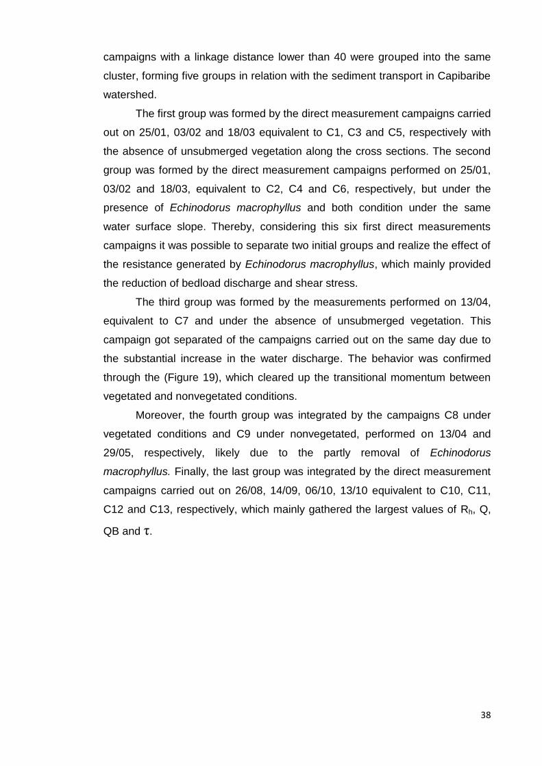
38

campaigns with a linkage distance lower than 40 were grouped into the same

cluster, forming five groups in relation with the sediment transport in Capibaribe

watershed.

The first group was formed by the direct measurement campaigns carried

out on 25/01, 03/02 and 18/03 equivalent to C1, C3 and C5, respectively with

the absence of unsubmerged vegetation along the cross sections. The second

group was formed by the direct measurement campaigns performed on 25/01,

03/02 and 18/03, equivalent to C2, C4 and C6, respectively, but under the

presence of Echinodorus macrophyllus and both condition under the same

water surface slope. Thereby, considering this six first direct measurements

campaigns it was possible to separate two initial groups and realize the effect of

the resistance generated by Echinodorus macrophyllus, which mainly provided

the reduction of bedload discharge and shear stress.

The third group was formed by the measurements performed on 13/04,

equivalent to C7 and under the absence of unsubmerged vegetation. This

campaign got separated of the campaigns carried out on the same day due to

the substantial increase in the water discharge. The behavior was confirmed

through the (Figure 19), which cleared up the transitional momentum between

vegetated and nonvegetated conditions.

Moreover, the fourth group was integrated by the campaigns C8 under

vegetated conditions and C9 under nonvegetated, performed on 13/04 and

29/05, respectively, likely due to the partly removal of Echinodorus

macrophyllus. Finally, the last group was integrated by the direct measurement

campaigns carried out on 26/08, 14/09, 06/10, 13/10 equivalent to C10, C11,

C12 and C13, respectively, which mainly gathered the largest values of Rh, Q,

QB and τ.

39

Figure 22. Dendrogram of classification for the thirteen direct measurement

campaigns.

40

6. CONCLUSIONS

1. The effect of resistance generated by Echinodorus macrophyllus mainly

influenced the bedload discharge, accounting for 37% of reduction in bed

load transport rate between the crosses sections studied in Capibaribe River.

2. The low ratio between bedload and suspended solid discharge, which ranged

from 0.18% to 3.51% with the mean value equal to 1.31% can be associated

to the presence of dams along the Capibaribe watershed.

3. Total variance of sediment transport rate explained by the first two principal

components equal to 90.03%, as well as the classification provided by

hierarchical cluster analysis for direct measurement campaigns under

vegetated and nonvegetated conditions showed the usefulness of

multivariate analysis.

4. The hydraulic roughness of the cross section vegetated by Echinodorus

macrophyllus was characterized through the mean vegetation drag

coefficient (CD’) equal to 4.02 m-1, demonstrating the adequacy of the method

applied in Capibaribe River.

41

7. REFERENCES

AGÊNCIA ESTADUAL DE MEIO AMBIENTE E RECURSOS HIDRÍCOS

(CPRH). Diagnóstico do meio físico e biótico e mapa do uso e ocupação do

solo do núcleo metropolitano do litoral de Pernambuco. Recife: CPRH/GERCO,

2006.

AGÊNCIA NACIONAL DE ÁGUAS (ANA). Boletim de monitoramento dos

reservatórios do Rio Capibaribe / Agência Nacional de Usos Múltiplos. Brasília.

v.1, p.1-27, 2010.

ARAÚJO, A. M.; COSTA, M. B. S. F.; MACÊDO, E. C.; CANTALICE, J. R. B.

Formas de fundo em águas costeiras e estudos de ondas e correntes locais. In:

VII Encontro Nacional de Engenharia de Sedimentos - VIII ENES, 2008, Campo

Grande/MS. Encontro Nacional de Engenharia de Sedimentos - VIII ENES.

Porto Alegre: ABRH, 2008.

ARAÚJO, A. M.; MINEIRO, A. L. B.; ATANÁZIO, C. M. C.; CANTALICE, J. R.

B.; SOUZA, W. L. S.; SILVA, Y. J. A. B. Estudo preliminar da descarga de

sedimentos do rio Beberibe/Pernambuco. In: IX Encontro Nacional de

Engenharia de Sedimentos - IX ENES, 2010, Brasília - DF. Encontro Nacional

de Engenharia de Sedimentos - IX ENES. Porto Alegre: ABRH, 2010.

BACK, A. J. Medidas de vazão com molinete hidrométrico e coleta de

sedimentos em suspensão. Boletim Técnico n.130. EPAGRI, Florianópolis –

SC. 58p, 2006.

BAKER, D. W., BLEDSOE, B. P., ALBANO, C. M., and POFF, N. L.

Downstream effects of diversion dams on sediment and hydraulic conditions of

rocky mountain streams. River research and applications, v.27, p.388-401,

2011.

BENNETT, S.J.; PIRIM, T.; BARKDOLL, B.D. Using simulated emergent

vegetation to alter stream direction within a straight experimental channel.

Geomorphology, v.44, p.115–126, 2002.

42

BUNTE, K. and S.R. Abt. Sampling surface and subsurface particle-size

distributions in wadable gravel and cobble-bed streams for analyses in

sediment transport, hydraulics, and stream-bed monitoring: U.S. Department of

Agriculture Forest Service Rocky Mountain Research Station General Technical

Report RMRS-GTR-74, 2001, 428p.

CARVALHO, N. O. Hidrossedimentologia prática, CPRM/Eletrobrás, Rio de

Janeiro, 1994, 352p.

CARVALHO, N. O. Hidrossedimentologia prática. 2° ed., rev., atual e ampliada.

Rio de Janeiro, 2008, 600p.

CARVALHO, N. O.; JÚNIOR, N. P. F.; SANTOS, P. M. C.; LIMA, J. E. F. W.

Guia de práticas sedimentométricas. ANEEL, Brasília-DF, 2000, 154p.

CHENG, L. Flow structure and sediment transport with impacts of aquatic

vegetation. Journal of Hydrodynamics, v.20, n.4, p.461-468, 2008.

CHENG, N. S. and NGUYEN, H. T. Hydraulic radius for evaluating resistance

induced by simulated emergent vegetation in open-channel flows. Journal of

Hydraulic Engineering, v.137, n.9, p.995-1004, 2011.

CLOUTIER, V.; LEFEBVRE, R.; THERRIEN, R.; SAVARD, M. M. Multivariate

statistical analysis of geochemical data as indicative of the hydrogeochemical

evolution of groundwater in a sedimentary rock aquifer system. Journal of

Hydrology, v.353, p.294–313, 2008.

CURVE EXPERT 1.3 for Windows. Universidad Federal do Rio Grande do Sulk

(URGS), 2005.

DIPLAS, P.; KUHNLE, J.; GLYSSON, D.; EDWARDS, T. Sediment Transport

Measurements, In: Sedimentation Engineering – Process, Measurements,

Modeling and Practice, Ed. Garcia, M. H. ASCE Manual and Report on

Engineering Practice. n.110, Reston, p.307-309, 2008.

43

EDWARDS, T. K. and GLYSSON, G. D. Field methods for measurement of

fluvial sediment. In: Techniques of Water-Resources Investigations of the U.S.

Geological Survey (USGS). Reston, Virginia, book 3, chapter C2, 97p, 1999.

EINSTEIN, H. A. The bedload function for sediment transportation in open

channel flows. Department of Agriculture, Soil Conservation Service. Technical

bulletin. n.1026, 79p, 1950.

FREY, P. and CHURCH, M. Bedload: a granular phenomenon. Earth Surface

Processes and Landforms, v.36, p.58–69, 2011.

GRAY, J. R. Sediment data collection techniques. U.S. Geological Survey

Training Course. Castle Rock and Vancouver, WA. 2005. CD-ROM.

GÜLER, C.; THYNE, G.; MCCRAY, J. E.; TURNER, A. K. Evaluation and

graphical and multivariate statistical methods for classification of water

chemistry data. Hydrogeology Journal, v.10, p.455–474, 2002.

GUY, H. P. Techniques of Water-Resources Investigations of the United States

Geological Survey (USGS). Fluvial sediment concepts. Inv., book 3, chapter C1,

55p, 1970.

HEIDEL, S. S. The progressive lag of sediment concentration with flood waves.

American Geophysical Union, v.37, n.1, p.56, 1956.

HOROWITZ, A. J. An evaluation of sediment rating curves for estimating

suspended sediment concentrations for subsequent flux calculations.

Hydrological Processes, v.17, p.3387–3409, 2003.

HOROWITZ, A. J. Determining annual suspended sediment and sediment-

associated trace element and nutrient fluxes. Science of the Total Environment,

v.400, p.315-343, 2008.

ISHIKAWA, Y.; SAKAMOTO, T.; MIZUHARA, K. Effect of density of riparian

vegetation on effective tractive force. J. For. Res, v.8, p.235–246, 2003.

44

JAMES, C. S.; GOLDBECK, U. K.; PATINI, A.; JORDANOVA, A. A. Influence of

foliage on flow resistance of emergent vegetation. Journal of Hydraulic

Research, v.46, n.4, p.536–542, 2008.

JAMES, C. S.; BIRKHEAD, A.L.; JORDANOVA, A.A.; KOTSCHKY, K.A.;

NICOLSON, C.; MAKOA, M.J. Interaction of reed distribution, hydraulics and

River morphology. Water Research Commission Report 856/1/01. Pretoria,

2001.

JAMES, C. S., BIRKHEAD, A.L., JORDANOVA, A.A., O'sullivan, J.J. Flow

resistance of emergent vegetation. Journal of Hydraulic Research, v.42, n.4, p.

390-398, 2004.

JÄRVELÄ, J. Flow resistance of flexible and stiff vegetation, a flume study with

natural plants. Journal of Hydrology, v.269, p.44–54, 2002.

JÄRVELÄ, J. Flow resistance in environment channels: Focus on vegetation.

2004, 54p. (Ph. D. Thesis). Helsinki University of Technology Water Resources

Publications.

JULIEN, P. Y. Erosion and sedimentacion. Melbourne: Cambridge University

press, 280p, 1995.

KAO, D. T.; BARFIELD, B. J.; LYONS, AUSTIN E. Hydraulic resistance of grass

media on shallow overland flow. University of Kentucky Water Resources

Research Institute Research Report, n.107, 97p, 1977.

KOTHYARI, U. C.; HAYASHI, K.; HASHIMOTO, H. Drag coefficient of

unsubmerged rigid vegetation stems in open channel flows. Journal of Hydraulic

Research, v.47, n.6, p.691–699, 2009.

LABORATÓRIO METEREOLÓGICO DE PERNAMBUCO (LAMEPE).

Disponível em: http://www.itep.br/LAMEPE.asp. Acessado: 26 de Setembro de

2011.

45

LEE, J. K.; ROIG, L. C.; JENTER, H. L.; VISSER, H. M. Drag coefficients for

modeling flow through emergent vegetation in the Florida Everglades.

Ecological Engineering, v.22, p.237–248, 2004.

JACOMINE, P. K. T. Levantamento exploratório - Reconhecimento de solos de

Pernambuco. Divisão de Pesquisa Pedológica (DNPE). Ministério da

Agricultura. Recife-PE, v.1, 359p, 1973.

LI, R. M. and SHEN, H. W. Effect of tall vegetations on flow and sediment.

Journal of the Hydraulics Division, ASCE v.99, n.5, p.793-814, 1973.

LINDNER, K. Flow resistance of vegetation. 1982. Mitteilungen 75. (Doctoral

thesis). Leichtweiss-Institut für Wasserbau. Technische Universität

Braunschweig.

MAHESHWARI, B.L. Suitability of different flow equations and hydraulic

resistance parameters for flows in surface irrigation: a review. Water Resources

Research, v.28, n.8, p.2059–2066, 1992.

MAYRINCK, O. M. A paisagem do rio Capibaribe: um recorte de significados e

representações. 2003. (Tese de Doutorado), Instituto de

Geociências/Universidade Federal do Rio de Janeiro.

MELO, R. O. Caracterização da produção de sedimentos de uma microbacia

no semi-árido pernambucano. 2008. 94p. (Dissertação) - Universidade Federal

Rural de Pernambuco, Recife.

MERTEN, G. H. and POLETO, C. Qualidade dos Sedimentos. Associação

Brasileira de Recursos Hídricos – ABRH. Porto Alegre, RS. 397p, 2006.

MEYBECK, M.; LAROCHE, L.; DURR, H. H.; SYVITSKI, J. P. M. Global

variability of daily total suspended solids and their fluxes in Rivers. Global and

Planetary Change, v.39, p.65–93, 2003.

46

NEPF, H. M. and VIVONI, E. R. Flow structure in depth-limited, vegetated flow.

Journal of Geophysical Research, v.105, n.C12, p.28,547-28,557, 2000.

NEPF, H. M. Drag, turbulence, and diffusion in flow through emergent

vegetation. Water Resources Research, v.35, n.2, p.479–489, 1999.

NEZU, I. and ONITSUKA, K. Turbulent structures in partly vegetated open

channel flows with LDA and PIV measurements. Journal of Hydraulic Research,

v.39, n.6, p.629–642, 2001.

PETRYK, S. and BOSMAJIAN, G. B. Analysis of flow through vegetation.

Journal of the Hydraulics Division, ASCE, v.101, n.7, p.871-884, 1975.

PRECISO, E.; SALEMI, E.; and BILLI, P. Land use changes, torrent control

works and sediment mining: effects on channel morphology and sediment flux,

case study of the Reno River (Northern Italy). Hydrological Processes.

Published online in Wiley Online Library. DOI: 10.1002/hyp.8202, 2011.

PONCE, V. M. Engineer Hydrology. Principles and Practices. Prentice-Hall, Inc.

New Jersey (1989). 640p.

SAEIDI, P.; TABATABAEI, J.; SAEDI, T. Effective discharge for suspended

sediment transportation in Ghohruod watershed. African Journal of Agricultural

Research, v.6, n.23, p. 5360-5366, 2011.

SIMONS, D. B.; SENTURK, F. Sediment transport technology. Colorado State

University. Fort Collins, CO. 1997. 897p.

SIMONS, D. B. and SENTURK, F. Sediment Transport Technology: water and

sediment dynamics. In: Water Resources Publications. [Colorado]: [s.n.], 879p,

1992.

SOUZA, W. L. S. Produção de sedimentos da bacia hidrográfica do rio

Capibaribe para zona costeira da região metropolitana do Recife. 2011. 136p.

(Dissertação) – Universidade Federal Rural de Pernambuco, Recife.

47

SUDENE. Dados Pluviométricos mensais do Nordeste. Estação de

Pernambuco: Recife. 1990. 363p.

TANINO, Y. and NEPF, H. M. Laboratory investigation of mean drag in a

random array of rigid, emergent cylinders. Journal of Hydraulic Engineering,

v.134, n.1, p.34–41, 2008.

THORNTON, C. I.; STEVEN, R.; MORRIS, C.E.; FISCHENICH, J.G.

Calculating shear stress at channel-overbank interfaces in straight channels

with vegetated floodplains. Journal of Hydraulic Engineering, v.126, p.929–936,

2000.

USDA - UNITED STATES DEPARTMENT OF AGRICULTURE. Soil Survey

Staff. Soil taxonomy: a basic system of soil classification for making and

interpreting soil surveys. 2nd ed. U.S. Department of Agriculture/Natural

Resources Conservations Service, Washington, Agriculture Handbook.1999.

871p.

USGS – United States Geological Survey. Techniques of Water Resources

Investigations. Washington, 1973.

USGS – United States Geological Survey. Techniques of Water Resources

Investigation. Washington, 2005.

WANG CHAO and WANG PEI-FANG. Flow structure of partly vegetated open-

channel flows with eelgrass. Journal of Hydrodynamics, v.21, n.3, p.301-307,

2009.

WILDE, F. D. and RADKE, D. B. Field Measurements In: National Field Manual

for the Collection of Water-Quality Data. U.S. Geological Survey Techniques the

Water Resource Investigations, book 9, chapter A4, p.7-99, 1998.

48

WU, F.C., SHEN, H. W., CHOU, Y.J. Variation of roughness for unsubmerged

and submerged vegetation. Journal of Hydraulic Engineering, v.125, n.9, p.

934–942, 1999.

YANG, C. T. Bedload Transport. In: Sediment Transport: theory and practice.

McGraw-Hill, 1996. p.90-121.

YEN, B. C. Open channel flow resistance. Journal of Hydraulic Engineering,

v.128, n.1, p.20-39, 2002.

ZIMA, L. and ACKERMANN, N. L. Wave generation in open channels by vortex

shedding from channel obstructions. Journal of Hydraulic Engineering, v.128,

n.6, p.596-603, 2002.

Date post:	08-Nov-2018
Category:	Documents
Upload:	lamtram
View:	216 times
Download:	0 times

INTERFERENCE OF HYDRAULIC ROUGHNESS GENERATED...

Documents