Page 1
Interference Suppression using MIMO
and Physical Layer Network Coding
Flávio André Silva Brás
Thesis to obtain the Master of Science Degree in
Electrical and Computer Engineering
Supervisors: Prof. António José Castelo Branco Rodrigues
Prof. Francisco António Taveira Branco Nunes Monteiro
Examination Committee
Chairperson: Prof. Fernando Duarte Nunes
Supervisor: Prof.Francisco António Taveira Branco Nunes Monteiro
Member of Committee: Prof. Mário Alexandre Teles de Figueiredo
April 2014
Page 3
iii
To my loved ones
Page 5
v
Abstract
This thesis chiefly deals with the concept of interference cancellation when a receiver knows
the channel that each of the interfering messages have gone through. This may be the case in “pure”
MIMO or when merging the concept of successive interference cancelation (SIC) with physical layer
network coding (PLNC), interpreting PLNC as a first stage of SIC.
This work begins by introducing the concept of PLNC through different approaches and
proceeds providing an overview of lattices, including basic and useful properties, since lattices take an
important place in this dissertation. MIMO detection problem is deeply discussed as a closest vector
problem (CVP) in a lattice and several low-complexity sub-optimal receivers are analysed, assessing
their performances.
Finally, this dissertation presents a set of new strategies combining MIMO with PLNC in
scenarios that move beyond the traditional two-way relay channel (TWRC), including the two time-
slots strategy with MIMO terminals in a network with a MIMO relay that can always be generalized
to scenarios with terminals, each of which equipped with antennas, and a MIMO relay
equipped with antennas, allowing the exchange of messages in just two time-slots.
Keywords
Lattices, MIMO Detection, Physical Layer Network Coding, Successive Interference Cancelation
Page 7
vii
Resumo
Esta dissertação lida principalmente com o conceito de cancelamento de interferência quando
um receptor sabe o canal pelo qual cada uma das mensagens que interferem passaram. Este pode ser o
caso de MIMO "puro" ou de quando se junta o conceito de cancelamento sucessivo de interferência
(SIC) com o de physical layer network coding (PLNC), interpretando PLNC como uma primeira fase
do SIC.
Este trabalho começa com a introdução ao conceito de PLNC através de diferentes
abordagens e prossegue dando uma visão geral de lattices, incluindo propriedades básicas e úteis, uma
vez que estes ocupam um lugar de destaque nesta dissertação. O problema de detecção em MIMO é
profundamente discutido como um problema de vector mais próximo (CVP) num lattice e vários
receptores sub-óptimos de baixa complexidade são analisados, avaliando os seus desempenhos.
Por último, este trabalho apresenta um conjunto de novas estratégias que combinam MIMO
com PLNC em cenários que vão para lá do two-way relay channel (TWRC), incluindo a estratégia de
dois time-slots com terminais MIMO numa rede com um relay MIMO que pode ser generalizada para
cenários com terminais, cada um dos quais equipado com antenas, e um relay MIMO
equipado com antenas, permitindo a troca de mensagens entre os terminais em apenas dois time-
slots.
Palavras-chave
Lattices, Detecção MIMO, Physical Layer Network Coding, Cancelamento Sucessivo de Interferência
Page 9
ix
Acknowledgments
First of all, I would like to thank Professor António Rodrigues for giving me the opportunity
to work on such a recent research topic, for his support and his good mood.
I am especially grateful to Professor Francisco Monteiro for being always available for any
issue concerning this work, for all the many weekly hours of supervision, for the numerous insightful
discussions that have so greatly enriched my knowledge of the field, for his contributions and advices
which greatly improved the quality of this dissertation and for his time spent reviewing this
manuscript as well as for providing me with his valuable feedback. This thesis could not exist without
his endless support.
A word of gratitude goes to my peer Filipe Ferreira for his shown interest, push forward
attitude and help to materialize the path followed by this dissertation.
I would not be at this stage of my life if it were not for my family. It is not enough to say
thank you for all the support but I hope I have made you feel proud.
Along the last years the passage of the days would have been neither so quick nor so
enjoyable without a number of friends that I met along the way. They know who they are and surely
know that I am close to the deadline. Nevertheless I would like to thank to Miguel Pereira and Igor
Duarte for helping me with the review of this dissertation, to Nelson Rodrigues and Pompeu Santos
for borrow me their laptops for simulations, to André Vieira and Bruno Neves. Seriously it has been a
great time.
Page 11
xi
Contents
Abstract ................................................................................................................................................... v
Resumo ................................................................................................................................................. vii
Acknowledgments .................................................................................................................................. ix
Contents ................................................................................................................................................. xi
List of Figures ...................................................................................................................................... xiii
List of Tables ........................................................................................................................................ xv
Acronyms ............................................................................................................................................ xvii
Symbols and Notation .......................................................................................................................... xix
Chapter 1 – Introduction to Physical Layer Network Coding .......................................................... 1
1.1 Overview ................................................................................................................................. 2
1.2 Compute and Forward ............................................................................................................. 7
Chapter 2 – Lattices .............................................................................................................................. 9
2.1 Context .................................................................................................................................. 10
2.2 Basic Definitions ................................................................................................................... 11
2.2.1 Lattice ............................................................................................................................... 11
2.2.2 Examples ........................................................................................................................... 12
2.2.3 Fundamental Region ......................................................................................................... 12
2.2.4 Voronoi Region ................................................................................................................. 14
2.2.5 Volume .............................................................................................................................. 15
2.2.6 Determinant ....................................................................................................................... 15
2.2.7 Bases ................................................................................................................................. 15
2.2.8 Successive Minima and Shortest Vector ........................................................................... 17
2.3 Lattice Reduction .................................................................................................................. 18
Page 12
xii
Chapter 3 – MIMO Detection ............................................................................................................ 21
3.1 MIMO Spatial Multiplexing ................................................................................................. 22
3.1.1 The Real Equivalent Model .............................................................................................. 27
3.1.2 The Closest Vector Problem ............................................................................................. 27
3.2 Maximum Likelihood Detection ........................................................................................... 29
3.3 Linear Equalization ............................................................................................................... 31
3.4 Order Successive Interference Cancellation Detection ......................................................... 36
3.5 Lattice Reduction-Aided Detection ...................................................................................... 41
Chapter 4 – MIMO combined with PLNC ....................................................................................... 49
4.1 System Model ....................................................................................................................... 50
4.2 MIMO combined with PLNC in TWRC ............................................................................... 56
4.3 PLNC in a Network with a MIMO Relay ............................................................................. 59
4.3.1 Two Time-slots Strategy ................................................................................................... 59
4.3.2 Three Time-slots Strategy ................................................................................................. 63
4.3.3 Two Time-slots Strategy with MIMO Terminals ............................................................. 67
Chapter 5 – Conclusions ..................................................................................................................... 71
5.1 Main Conclusions ................................................................................................................. 72
5.2 Future Work .......................................................................................................................... 73
References ............................................................................................................................................ 75
Page 13
xiii
List of Figures
TOC \h \z \c "Figure" Figure 1.1. Two-way relay channel scheme. ...................................................... 4
Figure 1.2. A traditional scheme for TWRC. .......................................................................................... 5
Figure 1.3. A network coding strategy for TWRC.................................................................................. 5
Figure 1.4. A PLNC strategy for the TWRC. ......................................................................................... 6
Figure 1.5. Nested lattices in CF strategy. .............................................................................................. 7
Figure 1.6. Reliably decoding an integer combination of the transmitted messages in CF strategy. ..... 8
Figure 2.1. Lattice illustrations lattice in ......................................................................................... 10
Figure 2.2. Examples of lattices in .. ................................................................................................ 13
Figure 2.3. Tilling of the with the fundamental region . ......................................... 14
Figure 2.4. Illustrations of Voronoi regions of two distinct lattices. .................................................... 14
Figure 2.5. Shortest vector .................................................................................................. 17
Figure 3.1. Point-to-point MIMO system. ............................................................................................ 24
Figure 3.2.Illustration of the -QAM constellations. ......................................................................... 25
Figure 3.3. Illustration of a simple example of CVP in . .................................................................. 28
Figure 3.4. ML detection with 2 2 antennas. ....................................................................................... 30
Figure 3.5. ML detection with 3 3 antennas. ....................................................................................... 30
Figure 3.6. Detection 2 2 antennas with 4-QAM using linear receivers. ............................................ 34
Figure 3.7. Detection 2 2 antennas with 16-QAM using linear receivers. .......................................... 34
Figure 3.8. Detection 3 3 antennas with 4-QAM using linear receivers. ............................................ 35
Figure 3.9. Detection 3 3 antennas with 16-QAM using linear receivers. .......................................... 35
Figure 3.10. Detection 2 2 antennas with 4-QAM using OSIC linear receivers. ................................ 39
Figure 3.11. Detection 2 2 antennas with 16-QAM using OSIC linear receivers. .............................. 39
Figure 3.12. Detection 3 3 antennas with 4-QAM using OSIC linear receivers. ................................ 40
Figure 3.13. Detection 3 3 antennas with 16-QAM using OSIC linear receivers. .............................. 40
Figure 3.14. Detection 2 2 antennas with 4-QAM using LRA linear receivers. ................................. 44
Figure 3.15. Detection 2 2 antennas with 16-QAM using LRA linear receivers. ............................... 44
Figure 3.16. Detection 3 3 antennas with 4-QAM using LRA linear receivers. ................................. 45
Figure 3.17. Detection 3 3 antennas with 16-QAM using LRA linear receivers. ............................... 45
Figure 3.18. Detection 2 2 antennas with 4-QAM using LRA OSIC linear receivers. ....................... 46
Figure 3.19. Detection 2 2 antennas with 16-QAM using LRA OSIC linear receivers. ..................... 46
Page 14
xiv
Figure 3.20. Detection 3 3 antennas with 4-QAM using LRA OSIC linear receivers. ....................... 47
Figure 3.21. Detection 3 3 antennas with 16-QAM using LRA OSIC linear receivers. ..................... 47
Figure 4.1. Simplified system diagram in discrete-time. ...................................................................... 52
Figure 4.2. Full system diagram in continuous-time............................................................................. 52
Figure 4.3. Distributed MIMO at the uplink phase. .............................................................................. 54
Figure 4.4. Uplink phase on MIMO combined with PLNC in TWRC. ................................................ 56
Figure 4.5. Downlink phase on MIMO combined with PLNC in TWRC. ........................................... 56
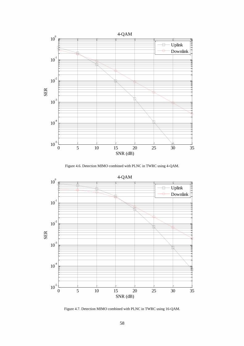
Figure 4.6. Detection MIMO combined with PLNC in TWRC using 4-QAM. ................................... 58
Figure 4.7. Detection MIMO combined with PLNC in TWRC using 16-QAM. ................................. 58
Figure 4.8. Uplink phase with 3 terminals. ........................................................................................... 59
Figure 4.9. Downlink phase on two time-slot strategy with 3 terminals. ............................................. 60
Figure 4.10. Detection two time-slot strategy with 3 terminals using 4-QAM. .................................... 62
Figure 4.11. Detection two time-slot strategy with 3 terminals using 16-QAM. .................................. 62
Figure 4.12. First time-slot from downlink phase on three time-slot strategy with 3 terminals. .......... 63
Figure 4.13. Second time-slot from downlink phase on three time-slot strategy with 3 terminals. ...... 63
Figure 4.14. Detection three time-slots strategy with 3 terminals using 4-QAM. ................................ 66
Figure 4.15 Detection three time-slot strategy with 3 terminals using 16-QAM. ................................. 66
Figure 4.16. Downlink phase on two time-slot strategy with 3 MIMO terminals. ............................... 67
Figure 4.17. OSIC-MMSE using 4-QAM in two time-slot strategy with MIMO terminals. ................ 69
Figure 4.18. OSIC-MMSE using 16-QAM in two time-slot strategy with MIMO terminals. .............. 69
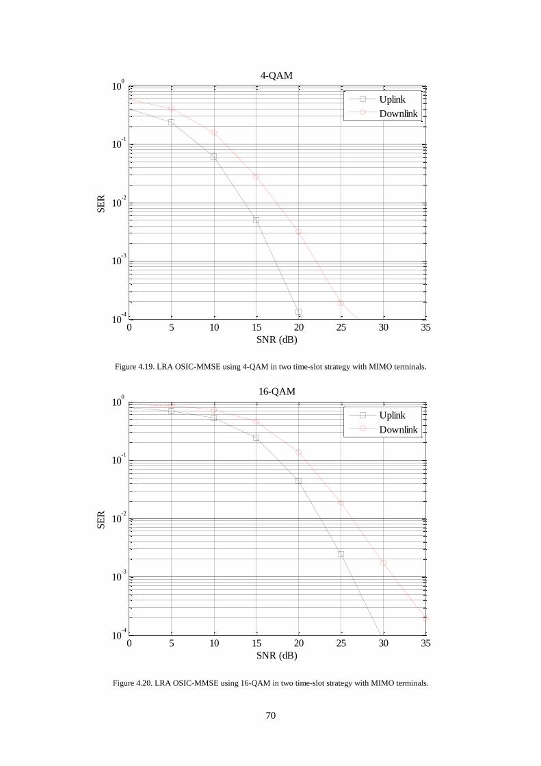
Figure 4.19. LRA OSIC-MMSE using 4-QAM in two time-slot strategy with MIMO terminals. ....... 70
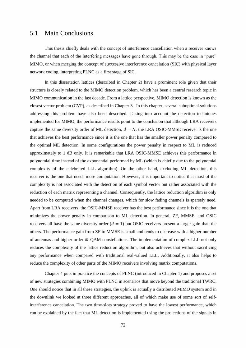
Figure 4.20. LRA OSIC-MMSE using 16-QAM in two time-slot strategy with MIMO terminals. ..... 70
Page 15
xv
List of Tables
Table 1. Wireless data standards and radio strategies used for multiplexing. ........................................ 3
Table 2. Pseudo-code of the complex LLL algorithm .......................................................................... 19
Table 3. Average symbol energy of modulations. ................................................................................ 26
Table 4 Pseudo-code of LRA detection. ............................................................................................... 42
Page 17
xvii
Acronyms
BER Bit error rate
BLAST Bell Laboratories Layered Space-Time Architecture
CDMA Code-division multiple access
CF Compute-and-forward
CLLL Complex LLL
CSIR Channel state information at the receiver
CVP Closest vector problem
DS Direct sequence
EM Electromagnetic
FDMA Frequency division multiple access
FH Frequency hopping
GSM Global System for Mobile Communications
KZ Korkine-Zolotareff algorithm
LLL Lenstra Lenstra Lovász algorithm
LRA Lattice reduction-aided
LST Layered Space-Time
LTE Long term evolution
MIMO Multiple-input multiple-output
Page 18
xviii
ML Maximum likelihood
MMSE Minimum mean square error
OFDM Orthogonal frequency division multiplexing
OSIC Ordered successive interference cancelation
PLNC Physical layer network coding
QAM Quadrature amplitude modulation
QPSK Quadrature phase-shift keying
SDMA Space-division multiple access
SIC Successive interference cancellation
SNR Signal-to-noise ratio
TDMA Time division multiple access
TWRC Two-way relay channel
UMTS Universal Mobile Telecommunications System
V-BLAST Vertical Bell Laboratories Layered Space-Time Architecture
WiMAX Worldwide Interoperability for Microwave Access
ZF Zero-forcing
ZMSW Zero-mean spatially white
Page 19
xix
Symbols and Notation
Symbols
Lattice generating matrix
Reduced lattice matrix
Constellation
Diversity order
Average energy of the complex symbol
Transmit filter
Receiver filter
Channel matrix
Extended matrix
Reduced channel matrix
Channel fading coefficient
Matched filter
Identity matrix
Rank of the lattice
Number of terminals
Unimodular matrix
Dimension of the lattice
Page 20
xx
Number of receive antennas
Number of transmit antennas
Additive noise vector
Symbol transmission period
Unitary matrix
Transmitted vector
Estimated vector with a certain detection technique
Receive filter for a certain detection technique
Messages from transmitter
Received vector
Extended vector
Small real number
Lattice
Noise variance
Variance (or power) of the constellations symbols
Notations
-dimensional complex space
-dimensional real space
-dimensional vectors with integer coordinates
Lattice generated by basis
Determinant of
Hermitian operator
Page 21
xxi
Transposition
Fundamental region of a lattice
Quantisation to constellation
Volume of a lattice
Voronoi region of a lattice
Imaginary part of a complex
Real part of a complex
Pseudo-inverse matrix
Hermitian matrix
Page 23
1
Chapter 1
Introduction to
Physical Layer Network Coding
This chapter gives a brief overview of the work. It is
presented an introduction to Physical Layer Network
Coding and its basic concept followed by a short
overview over the Compute-and-Forward strategy.
1 Introduction to Physical Layer Network Coding
Page 24
2
1.1 Overview
In recent years mobile communications have known great technological developments that
have had important social and economical impacts. This importance has resulted, among many other
things, in an exponential growth of the number of wireless devices as well as in increasingly richer
multimedia applications which have leading these devices to require higher and higher data rates.
These trends, combined with the fact of a limited spectrum, point to the conclusion that interference
between devices will be one of the dominant bottlenecks in wireless networking.
At the physical layer of wireless networks all data are transmitted through electromagnetic
(EM) waves and this means that when a wireless node transmits, the EM signals are often received by
more than one node. At the same time, a receiver may be receiving EM signals by a set of others
nodes simultaneously. These characteristics may cause interference among signals and traditionally
communications systems designs try to either reduce or avoid it. In Wi-Fi networks, for example,
when multiple nodes transmit together, packet collisions occur and none of the packets can be
received correctly.
Cellular networks are wireless networks distributed over land areas called cells, each served
by at least one base station. In this multiuser communications scenario the spectrum that can be used
is limited and, additionally, spectrum licensing is very expensive. Therefore, the design of wireless
systems has to be as spectrally efficient as possible. As it was emphasized in the previous paragraph,
at the physical and medium access layers the main issue in wireless networks is the management of
multiple access and interference. In this scenario the overall resources have to be shared by the users
and for doing that there are two natural strategies for separating resources between them, based on the
orthogonality principle (in either time or frequency domain), thus avoiding interference between
them. One of these strategies is time division multiple access (TDMA), which separates the
transmissions to and from different users in time, introducing the concept of time-slot as the finest
divisible resource allocated to a user. The other one is frequency division multiple access (FDMA)
which achieves the separation in the frequency domain. These two strategies assure a multiple access
of the channel by the users and also separate the uplink (from the terminals to a base station) from the
downlink (from the base station to the terminals).Standards such as GSM are a prime example of the
implementations of these two strategies.
Transmissions in the same band and overlapping in time are also possible. Code-division
multiple access (CDMA) base direct sequence (DS) spread spectrum consists in assigning different
orthogonal spreading sequences to different users, and thus each user ends up using all the bandwidth
available. Note that this is just another manner of implementing orthogonal signalling. When a user in
CDMA is demodulating its data, the other users’ signals appear as pseudo white noise. Universal
frequency reuse is a key property of CDMA systems because all cells use the same spectrum which
Page 25
3
eliminates the need for frequency reuse cell planning. Another way for implementing CDMA is by
means of frequency hopping (FH). FH is an alternative spread spectrum technique to DS where a
signal periodically changes its carrier frequency according to a pseudo-random sequence of different
frequencies.
All the strategies mentioned above were initially applied to single-carrier systems. Overtime
most wireless systems are adopting orthogonal frequency division multiplexing (OFDM) as the
modulation scheme, where a symbol stream is parallelised over a given bandwidth using adjacent
orthogonal frequencies. This is particularly beneficial for frequency selective wireless channels
because each one of the sub-streams is transmitted over a narrow-band where the fading is almost flat.
Long term evolution (LTE) combines ideas related to TDMA and FDMA combined with
OFDM using the concept of time-frequency resource-blocks that a user can use over time [1].
The advent of multiple-input multiple-output (MIMO) was the key technique to increase the
spectral efficiently in wireless transmission. These systems take advantage of space-dimension which
lead to the concept of space-division multiple access (SDMA). Along with physical layer network
coding (PLNC), MIMO detection will be the main focus of this dissertation, furthermore a set of new
strategies combining these two concepts will be proposed in Chapter 4.
Table 1 summarises which are the wireless strategies used in the most common commercial
wireless data standards [2].
Table 1. Wireless data standards and radio strategies used for multiplexing.
Wireless data standard Wireless techniques used
GSM TDMA / FDMA
UMTS CDMA / FDMA / MIMO
LTE OFDM / MIMO / SC-FDMA
Wi-Fi OFDM / MIMO
The strategies introduced until now face interference as a difficulty to communications.
Nevertheless it is actually possible to enable more efficient communications over a network making
use of interference in many scenarios. A new concept to further enhance the capacity of wireless
networks has recently emerged, it is the so-called physical layer network coding (PLNC). It appears to
have been independently proposed by several research groups in 2006: Zhang, Liew and Lam [3],
Page 26
4
Popovski and Yomo [4], and Nazer and Gastpar [5]. It was presented as a way to exploit the network
coding that occurs in Nature when multiple EM waves come together within the same physical space
and they add. This mixing of EM waves is indeed a form of network coding, this time performed by
Nature. So these authors instead of considering interference as a difficulty to be avoided, they rather
put it to a good use in order to improve throughput.
The scheme in [3] assumes a very simple channel model for intermediate nodes, in which the
received signal is a sum of two binary-modulated signals plus a Gaussian noise and intermediate
nodes try to decode the modulo-two sum of the transmitted messages. It is proved that this simple
strategy significantly improves the throughput of the two-way relay channel (TWRC).
In [4] the main idea is the same but a more general channel model is taking into account and
the received signal is given by , where and are the signals, is the Gaussian
noise and and are known complex-valued channel gains that captures the effects of fading and
imperfect phase alignment. It is shown that, in a large range of signal-to-noise ratios (SNR), the
strategy in [4] outperforms conventional relaying strategies (such as amplify-and-forward and decode-
and-forward) for a two-way relay channel.
The framework by Nazer and Gastpar [5] moves beyond two-way relay channel and will be
presented in the next section.
The TWRC is just one of the many scenarios where the broadcast property of the wireless
medium can be exploited via network coding and now it will be used to better illustrate the idea of
PLNC, this example first appeared in a paper by Wu et al. in 2004 [6].
Let us consider two nodes which cannot hear the transmissions of each other and in order to
communicate they are helped by a relay that can hear and transmit to both (Figure 1.1). A practical
example of this configuration is a satellite network in which nodes 1 and 2 are the ground stations,
and the relay is the satellite. It is assumed that the nodes share the same frequency band and it is
imposed a half-duplex constraint which means that each terminal just can send or receive during a
single time-slot.
Figure 1.1. Two-way relay channel scheme.
The usual proposal of this situation is the following: node 1 wants to send the message to
node 2 and that node 2 wants to send a message to node 1, or shortly node 1 and node 2 wants to
exchange messages. With the assumptions made if the nodes transmit at the same time the relay will
observe a superposition of the two signals corrupted by noise. The traditional scheme with a design
Node 1 Node 2RelayHas w1
Wants w2
Has w2
Wants w1
Page 27
5
principle that tries to avoid interference and without the use of network coding requires four time-slots
to exchange messages as illustrated in Figure 1.2.
Figure 1.2. A traditional scheme for TWRC.
In this four time-slot strategy each terminal takes one time-slot to transmit its message and
then the relay takes more two time-slots to distribute the messages.
By applying pure network coding, the number of time-slots can be reduced to three as
illustrated in Figure 1.3. By reducing the number of time-slots from four to three, the use of network
coding has a throughput improvement of 33% over the traditional scheme.
Figure 1.3. A network coding strategy for TWRC.
Node 1 Node 2Relay
w1
Node 1 Node 2Relay
Node 1 Node 2Relay
Node 1 Node 2Relay
Time slot 1
Time slot 2
Time slot 3
Time slot 4
w2
w1
w2
Node 1 Node 2Relay
w1
Node 1 Node 2Relay
Node 1 Node 2Relay
Time slot 1
Time slot 2
Time slot 3
w2
w1 w2
Page 28
6
This strategy is a straightforward way of applying network coding. Initially node 1 sends its
message to the relay on time-slot one and then node 2 also sends its message to the relay on the
second time-slot. Then the relay compute the sum of the messages ( ) and in the third time-slot
it sends this sum to both nodes. So its visible that is more efficient if the relay sends the sum of the
messages in the broadcast phase what suggest the idea that if it would be possible save time-slots in
the multiple-access phase too. Since the relay only needs the sum of the signals we can
simultaneously transmit them to the relay at the same time. This is done using PLNC and it reduces
the number of time-slots to two as shown in Figure 1.4. It allows nodes 1 and 2 to transmit in the same
time-slot and exploits the network coding operation performed by nature where the transmitted signals
are added up on the wireless channel. This property can be exploited to send the sum or another linear
function to the relay in a single time-slot. By doing so, PLNC can improve the performance of TWRC
by 100%.
Figure 1.4. A PLNC strategy for the TWRC.
In this strategy of PLNC it is assumed symbol-level and carrier-level synchronization, and
also the use of power control in order to packets from nodes 1 and 2 arrive at relay with the same and
amplitude.
To date, most works on PLNC have focused on TWRC. However many investigations on its
extension to the multi-way relay channel have been made where a relay or a system of relays
interconnects more than two end nodes. An example of that is the work of Chen Feng, Danilo Silva
and Frank R. Kschischang [7].
As a last note it is important to refer that although PLNC have been originally conceived for
application in wireless networks, network coding operations abound in nature. In fact, any physical
phenomenon in which an output is the function of a number of inputs can be exploited in the network
coding construct. So the application of PLNC could potentially be extended to many other domains
such as optical networks [8].
Node 1 Node 2Relay
w1
Node 1 Node 2Relay
Time slot 1
Time slot 2
w1 w2
w2
Page 29
7
1.2 Compute and Forward
The strategy proposed by Nazer and Gastpar [5] is another branch of PLNC. It is called
compute-and-forward (CF) and enables relays to decode linear equations of the transmitted messages
using noisy linear combinations provided by the channel. If a destination gets sufficiently linear
combinations it can solve these linear equations in order to obtain the desired messages.
Compute-and-forward simultaneously affords protection against noise and the opportunity to
exploit interference for cooperative gains. This strategy relies on codes with a linear structure,
specifically nested lattices codes, which ensures that integer combinations of codewords are
themselves codewords [9]. The lattice code should have some form of modulo arithmetic so that we
can map between the linear combination taken by the channel and our desired combination over the
messages. This property is satisfied by nested lattices which are a subset of another lattice, called the
fine lattice. The nested lattice can be replicated tilling the entire fine lattice. Lattices will be presented
in Chapter 2, however nested lattices are not discussed so Figure 1.5 illustrates a simple example of its
concept through a system were two transmitters send a message at the same time and frequency to a
receiver. In Figure 1.5 each transmitter maps its finite-field message into an element of the nested
lattice code and sends this vector on the cannel. Here, the channel coefficients ( and ) are taken to
be equal to 1. Therefore, the receiver observes a noisy sum of the transmitted vectors and determines
the closest lattice point. After taking a modulo operation with respect to the nested lattice, the receiver
can invert the mapping and determine the modulo sum of the original messages [10].
Figure 1.5. Nested lattices in CF strategy.
Page 30
8
More generally as depicted in Figure 1.6, considering terminals and a relay this strategy can
be roughly described as follows: each one of the terminals takes messages from a finite field, map
them onto nested lattice points, and transmit these across the channel. The relay observes a linear
combination of these lattice points and attempts to decode an integer combination of them. This
equation of lattice points is finally mapped back to a linear equation over a finite field. When the relay
gets different linear equations it can decode the desired messages [11].
Figure 1.6. Reliably decoding an integer combination of the transmitted messages in CF strategy.
Page 31
9
Chapter 2
Lattices
This chapter provides an overview of lattices
including basic and useful properties in a more
formal definition.
2 Lattices
Page 32
10
2.1 Context
Lattices are regular arrangements of points in Euclidean space, or in other words, they are a
set of points in -dimensional space with a periodic structure, such as the ones illustrated in Figure
2.1. Three dimensional lattices occur naturally in many settings such as crystals or in a stack of
oranges. Historically, lattices were investigated since the late 18th century by mathematicians such as
Lagrange, Gauss and later Minkowski, and was about the publication of the last one, Hermann
Minkowski, called Geometrie der Zahlen in 1896 that lattices have become a standard tool in number
theory, especially in the areas of algebraic number theory and the arithmetic theory of quadratic forms
for instance. Going forward in time, a significant advance in the algorithmic theory of lattices of
general rank occurred in the early 1980’s, with the development of the powerful lattice basis reduction
algorithm that came to be called the LLL (Lenstra Lenstra Lovász) algorithm that has found numerous
applications in both pure and applied mathematics. A complex-value version of this famous algorithm
will be presented later on in this chapter.
Lattices have now many applications in computer science and mathematics. Among many
others applications they are helpful to the solution of integer programming problems, cryptanalysis,
diophantine approximations and the design of error correcting codes for multi-antenna systems. More
recently, one of the most promising applications and that has attracted much attention is the use of
lattices as a source of computational hardness for the design of secure cryptographic functions.
Another promising application of lattices is its use as basis for coding schemes, and that
application is the one that will be explored. In the present work lattices take a prominent place as it
will become clearer in the next chapters so it is important to define this structure and understand its
main properties.
Figure 2.1. Lattice illustrations lattice in
Page 33
11
2.2 Basic Definitions
In this subsection it will be presented a more formal definition of lattice as well as its most
important mathematical properties based on [12] and [13].
2.2.1 Lattice
There are several ways of specifying a lattice. One of the definitions says that a lattice is a
discrete additive subgroup of , i.e., it is a subset satisfying the following properties:
- (group) is closed under addition and subtraction,
- (discrete) There is an such that any two distinct lattice points are at
distance at least
Note that not every subgroup of is a lattice. For example the subgroup is not a lattice
because it not fulfils the second property while the group is a lattice because integer vectors can be
added and subtracted obtaining again an integer vector, and clearly the distance between any two
integer vectors is at least one.
An equivalent definition of lattices can be obtained from by applying a linear
transformation. To illustrate this definition let’s consider a matrix that has full column rank,
what means that the columns of this matrix are linearly independent, and then
is also a lattice. Obviously this set is closed under addition and subtraction, besides it is also discrete.
Moreover all lattices can be expressed as for some what leads to the following definition.
Let where are linearly independent vectors in . The lattice
generated by is the set of all the integer linear combinations of the columns of ,
(2.1)
The matrix is called a basis for the lattice . The integer is called the dimension of the
lattice; the integer is the rank of the lattice and in the case of , is called a full rank
lattice.
In this second definition lattices can be represented by a basis matrix , containing integer or
rational entries, which generate the lattice. It is important to keep in mind this definition because it
will be present during all the work. The definition can be extended to complex lattices, however it is
possible to transform any complex lattice into a real lattice through the real equivalent model, so the
descriptions about lattices will continue with real lattices.
Page 34
12
A lattice is the span of a finite set of vectors in Euclidean space:
(2.2)
Notice the similarity between the definitions of a lattice and the span of a set of vectors :
(2.3)
The central difference is that in a lattice only integer coefficients are allowed, resulting in a
discrete set of points. As vectors are linear independent, any point can be
written as a linear combination in a unique way. Therefore if and
only if .
Notice that the definition can be extended to matrices whose
columns are not linearly independent. However, in this case, the resulting set of points is not always a
lattice because it may not be discrete.
2.2.2 Examples
In order to illustrate the next definitions it will be shown some examples. In the following
examples the fulfilled points are the ones that belong to the lattice. Besides these examples only
contain a part of the lattice but is intuitive to imagine how they span to the remaining space. Figure
2.2 a) represents a lattice generated by the vectors and which is the lattice of all
integers’ points, . As it is possible to see in Figure 2.2 b) the basis and also
generate moreover these bases are not unique, fact that will be explained later on in this chapter on
section 2.2.7 (Bases). On the other hand Figure 2.2 c) doesn’t generate , its basis and
generate instead a lattice of all integer points whose coordinates sum to an even number. Apart from
the other examples that are full-rank lattices Figure 2.2 d) represents a lattice of dimension 2 and rank
1 generated by the base .
2.2.3 Fundamental Region
For any lattice basis the fundamental region or parallelepiped is defined as
(2.4)
Notice that depends on the basis and it is easy to imagine that if we place one copy of
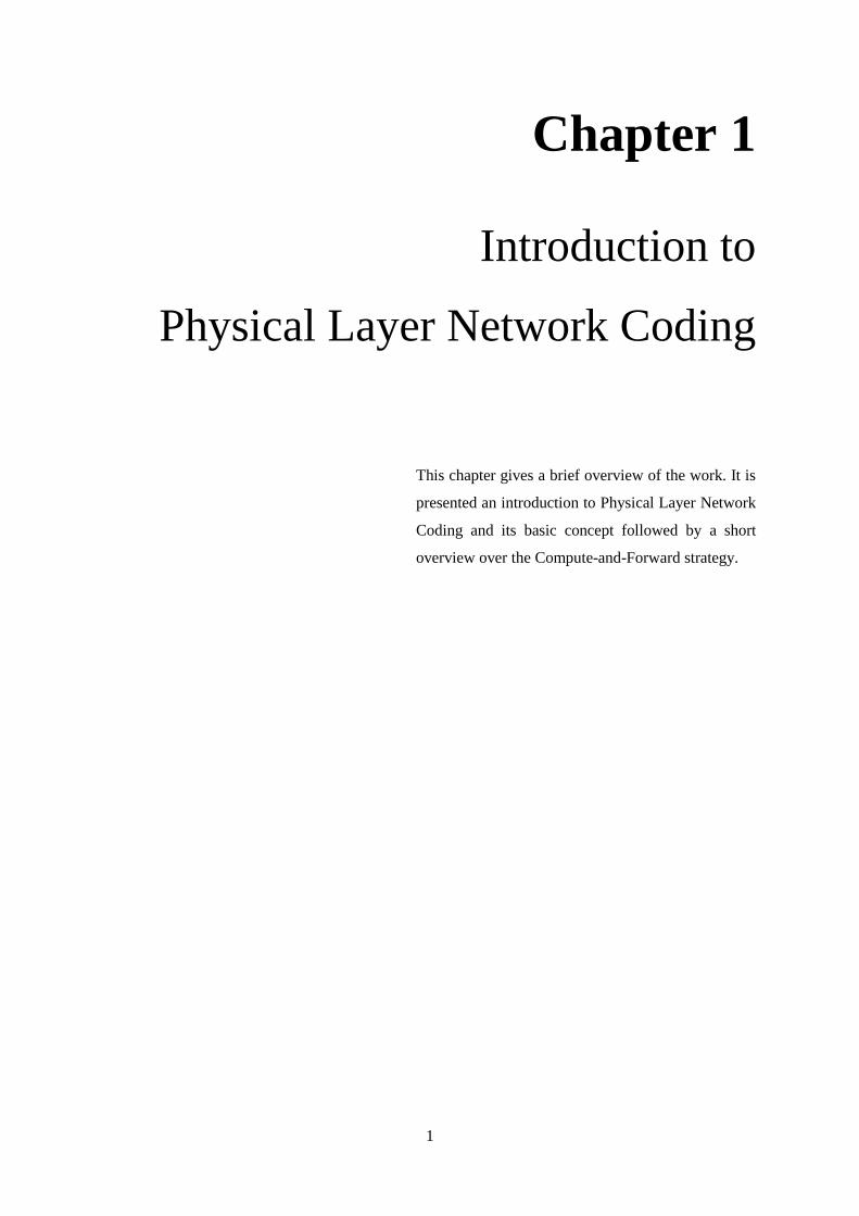
at each lattice point in we obtain a tiling of the entire as shown in Figure 2.3.
Page 35
13
In Figure 2.2 and Figure 2.3 the fundamental regions are represented by the shaded areas. In
Figure 2.3 are used two different shades just for a better illustration of the tilling of the space but they
represent the same area, i.e. the same fundamental region.
Based on the definition of the fundamental region it is possible to determine if a set of vectors
forms a basis of a lattice. As it shown above in the examples, not every set of n linearly vectors in
is a basis of and this is possible to determine following the next lemma: the fundamental region
generated by the vectors should not contain any lattice points, except the origin. For example, notice
that the fundamental regions in Figure 2.2 a) and Figure 2.2 b) do not contain any nonzero lattice
points and so they are bases of , however the fundamental region of Figure 2.2 c) contains the
lattice point and so the vectors that generate this lattice are not a basis of .
Figure 2.2. Examples of lattices in . (a) Lattice generated by basis and . (b) Lattice generated by basis
and . (c) Lattice generated by basis and . (d) Lattice generated by basis .
(a) (b)
(c) (d)
[1,1]
[1,1]
[2,1]
[0,1]
[1,0]
[2,0]
[2,1]
Page 36
14
Figure 2.3. Tilling of the with the fundamental region .
2.2.4 Voronoi Region
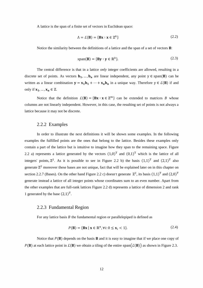
The Voronoi region is defined by
(2.5)
This equations defines the Voronoi region, which consists of the space where the lattice exists
that contains all the points in the span of the lattice which are closer to a given lattice point than to
any other point in the lattice. This region is a characteristic of the lattice and independent of any
particular generating matrix and it is the most interesting fundamental region that tiles the entire space
once it constitutes the optimal decision region for the closest vector problem (CVP) in a lattice, a
problem that will be discussed in the next chapter.
Figure 2.4 shows the tilling of two distinct lattices with its respective Voronoi region. As it is
intuitive from the figure the Voronoi regions are limited by the solid lines and they can assume many
forms.
Figure 2.4. Illustrations of Voronoi regions of two distinct lattices.
[2,0]
[1,1]
Page 37
15
2.2.5 Volume
In the case of full-rank lattices the volume of the lattice (that it is the same of the volume of
any of its many possible fundamental regions) is
(2.6)
however, in general the following expression is required:
(2.7)
In the complex case the Hermitian operator replaces transposition in the equation above. The
volume of the lattice is an invariant of the lattice, i.e., is independent of the choice of basis.
2.2.6 Determinant
Let be a lattice of rank . The determinant of , denoted , as the -
dimensional volume of the fundamental region . In symbols, this can be written as
. In the special case that is a full rank lattice, is a square matrix, and it stays that
.
The determinant of a lattice is an invariant of the lattice, in the sense that it is also
independent of the choice of basis . Indeed, if and are two bases of , then as it will be
presented next for some unimodular matrix . Hence,
(2.8)
The determinant of a lattice is inversely proportional to its density, what means that the
smaller the determinant, the denser the lattice is.
2.2.7 Bases
In the sub-section 2.2.3 (Fundamental Region) it was presented a lemma to verify if a basis
can be a basis of a certain lattice based on the fundamental region that the vectors of the basis create.
Now let us present it in a more formal way.
Let be a lattice of rank , and let be linearly independent lattice vectors.
Then form a basis of if and only if .
Proof. Assume first that form a basis of . Then, by definition, is the set of all
their integer combinations. Since is defined as the set of linear combinations of
Page 38
16
with coefficients in the range , the intersection of the two sets is .
For the other direction, assume that . Since is a rank lattice and
are linearly independent, we can write any lattice vector as for some .
Since by definition a lattice is closed under addition, the vector is also in . By
our assumption, . This implies that all are integers hence is an integer combination of
Note that different set of vectors may generate the same lattice but all these different bases are
related by unimodular transformations as it will be described below.
Let and be two bases. Then if and only if there exists a unimodular
matrix such that .
A matrix is called unimodular if it is a square matrix with integer entries and
determinant . The inverse of a unimodular matrix is also unimodular.
Proof. First assume for some unimodular matrix . Notice that if is unimodular,
then is also unimodular. In particular, both and are integer matrices, and and
. It follows that and , i.e., the two bases and are
equivalent and they generate the same lattice.
Now assume and are two bases for the same lattice . Then, by
definition of lattice, there exist integer square matrices and such that and .
Combining these two equations appears , or equivalently, . Since
vectors are linearly independent, it must be , i.e., . In particular,
. Since matrices and have integer entries,
, and it must be .
A simple way to obtain a basis of a lattice from another is to apply (a sequence of) elementary
column operations, as defined bellow. It is easy to see that elementary column operations do not
change the lattice generated by the basis because they can expressed as right multiplication by a
unimodular matrix. Elementary column operations are:
Swap the order of two columns in .
Multiply a column by .
Add an integer multiple of a column to another column: where and
.
Moreover, any unimodular transformation can be expressed as a sequence of elementary integer
column operations.
Page 39
17
2.2.8 Successive Minima and Shortest Vector
One basic parameter of a lattice is the length, meaning the Euclidean norm, of the shortest
nonzero vector in the lattice. This parameter is denoted by .
An equivalent way to define is the following. It is the smallest such that the lattice points
inside a ball of radius span a space of dimension 1 as is shown in Figure 2.5. This definition leads to
the following generalization of known as successive minima.
Let be a lattice of rank . For it is define the ith
successive minimum as
(2.9)
where is the closed ball of radius around 0.
Figure 2.5. Shortest vector
Page 40
18
2.3 Lattice Reduction
The idea of lattice reduction consists in changing a basis of a lattice into a shorter basis
such that remains the same. This process can be used to solve the shortest vector problem
however for high rank basis there is no known algorithm that finds the shortest vector in polynomial
time.
Lattice reduction can be implemented by algorithms such as LLL and KZ being the former
the most known. The LLL lattice basis reduction algorithm was invented by Arjen Lenstra, Hendrik
Lenstra and László Lovász in 1982 [14] and is a polynomial time lattice reduction algorithm. LLL
usually obtains an approximation for the shortest vector but as it was mentioned there is not any
efficient algorithm to solve this problem anyway the approximation obtain by the LLL is enough for
many applications. In this dissertation a complex version of the original LLL algorithm (CLLL) will
be used to assist a detection process in a receiver (see section 3.5).
In sub-section 2.2.7 were presented simple techniques to obtain different bases that generate
the same lattice, where one of those is to swap the order of two vectors in which is equivalent to
apply a unimodular transformation. Roughly speaking what LLL algorithm does is to perform
successive orthogonal projections and if necessary uses the technique of swapping two consecutives
vectors of , in order to get a reduced or near orthogonal basis . So the output of the algorithm is
a new basis consisting of near-orthogonal vectors and a unimodular matrix such that
In this dissertation, as mentioned, and based on [15] a complex version of this algorithm was
adopted since it reduces the complexity of the implementation without sacrificing any performance.
The detailed pseudo-code, using Matlab notation, of the algorithm implemented is presented in Table
2. Notice that parameter controls the performance and the complexity of the algorithm, i.e., higher
values of corresponds to higher complexity leading to a better performance. At the simulations
performed along this dissertation was assumed to be 0.75 as advised in literature. Since in the
following chapters basis of the lattice will be considered as the matrix of the channel coefficients
(see section 3.1) the pseudo-code will use the latter nomenclature.
Page 41
19
Table 2. Pseudo-code of the complex LLL algorithm
Input:
Output:
1:
2:
3:
4:
5:
6:
7:
8:
9:
10:
11:
12:
13:
14:
15: swap the
16:
17:
18:
19:
20:
21:
22: end
23: end
24:
Page 43
21
Chapter 3
MIMO Detection This chapter presents the MIMO detection problem
as a closest vector problem (CVP) in a lattice and
describes and analyses several low-complexity sub-
optimal receivers, assessing their performances.
3 MIMO detection
Page 44
22
3.1 MIMO Spatial Multiplexing
As it was described in Chapter 1 system designers are facing a number of challenges. The
limited availability of the radio frequency spectrum, a complex space-time varying wireless
environment and the increasing demand for higher data rates are some of these challenges. In recent
years Multiple-Input Multiple-Output (MIMO) systems have emerged as one of the most promising
technologies to answer to these challenges. MIMO communications systems can be defined by the use
of multiple antennas in the transmitting node as well as in the receiving node. The core idea behind
this strategy is that signals sampled in the spatial domain at both ends are combined in such a way that
they either create effective multiple parallel spatial data pipes, increasing the data rate, and/or adding
diversity to improve the quality of the communications by reducing the bit-error rate (BER).
MIMO spatial multiplexing has indeed allowed unprecedented spectral efficiencies in
wireless fading channels achieving high date-rates. However this gain of performance comes at a
price that is the high complexity of the detection in the receivers. This complexity has posed a great
challenge to decoder’s implementation and the present chapter will focus on the most part of the
receivers that have been implemented so far. The performance of linear receivers will be analysed, as
well as the successive interference cancellation (SIC) receiver and finally receivers with lattice
reduction, but before entering into the specifications of both the receivers and the work developed
itself it is important to present a background on MIMO as well as some models and problems
definitions.
The use of multiple antennas at both the transmit and receive nodes has become one of the
most important paradigms for the deployment of existing and emerging wireless communications
systems. The importance of MIMO systems is witnessed by their presence in many recent standards.
MIMO along with orthogonal frequency division multiplexing (OFDM) technology sustains the
physical layer of the fourth generation (4G) wireless networks such as LTE and also the LTE-
Advanced release, the latest generation of Wi-Fi, IEEE 802.11.n and Worldwide Interoperability for
Microwave Access, known as WiMAX (IEEE 802.16m standard).
Clearly, the benefits from multiple antennas arise from the use of the space dimension that
comes as a complement to time and because of that MIMO technology is also known as space-time
wireless or smart antennas. Still MIMO concept is not a new idea. Until the 1990s, the use of antenna
arrays at one node of the link was mainly oriented to the estimation of directions of arrival as well as
diversity, leading to beamforming and spatial diversity. Beamforming is a powerful technique which
increases the link signal-to-noise ratio (SNR) through focusing the energy into desired directions. The
concept of spatial diversity is that, in the presence of random fading caused by multipath propagation,
the SNR is significantly improved by combining the output of decorrelated antenna elements. In the
early 1990s new proposals for using antenna arrays to increase the capacity of wireless links enhanced
Page 45
23
enormous opportunities beyond diversity alone. It turned out that diversity was only the first step
towards mitigating multipath propagations. With the emergence of MIMO systems, multipath was
effectively converted into a benefit for the communications system. MIMO takes advantage of
random fading, and possibly delay spread, to multiply transfer rates [2].
One of the first examples of practical application of MIMO is the patent of Paulraj and
Kailath [16] which introduced a technique for increasing the capacity of a wireless link using multiple
antennas at both ends for application to broadcast digital TV.
Another relevant contribution appeared in 1996 in the paper of Foschini [17] where he
introduces the concept of Layered Space-Time (LTS) architecture. This architecture was later referred
as Bell Laboratories Layered Space-Time Architecture (BLAST) and it was designed for a point-to-
point MIMO communication system where the data stream generated by the source was divided in
several branches and encoded without sharing any information with each other. To solve some
limitations of its first release a new version of BLAST architecture was proposed in [18] and it was
called Vertical Bell Laboratories Layered Space-Time Architecture (V-BLAST). One of the most
important results of this kind of architecture is that, under some fading conditions, independent data
streams can be simultaneously transmitted over the matrix channel [19]. Motivated by the results of
Foschini, a large number of papers appeared in the open literature addressing the different aspects of
the MIMO architectures. Further progress in MIMO concepts came up with the paper of Viswanath,
Tse, and Anantharam [20], which was one of the first contributions addressing MIMO multiple-access
channels.
Other important topics in wireless communications have been investigated since 2000 but the
interest in MIMO topics has always been high. While earlier MIMO work focused on single user
applications (transmitter to single receiver or vice versa), MIMO are now expanding to multiuser
(transmitters to multiple receivers) and network applications (multi-transmitters to a single receiver).
These applications offer new challenges in coding channel spanning models to transmit as well as
decoding techniques at the receiver’s end [21].
Nowadays large MIMO systems and massive MIMO systems are a promising concept that
has attracted the research community, where the number of antennas is large ( 8) in the former and
very large in the latter. This approach uses compact antennas and claims to support huge performance
gains while still allowing fast iterative receiver decoding [22].
The type of MIMO system that will be discussed in this chapter is a point-to-point
communications MIMO, as illustrated in Figure 3.1. This system is based on multiple antenna
scenarios where both the transmitter and the receiver use several antennas, each one with separate
radio frequency modules, and where the interfering channels are the radio links between all pair of
transmit and receive antennas.
Page 46
24
Figure 3.1. Point-to-point MIMO system.
This kind of setup is chiefly considered for semi-mobile local-area wireless data
communications. As an example, the reader could think of a laptop computer equipped with a set of
antennas communicating with an access point, also equipped with several antennas.
In this MIMO communications system with transmit antennas and receive antennas
(with so that the linear system it gives rise to is determined) the relation between the
transmitted and received signals can be modelled in the baseband as
(3.1)
where is the received signals vector and
is the
transmitted signals vector. The radio links between each pair of transmit and receive antennas are
represented by the channel matrix in which its entries represent the complex
coefficient associated with the link between the pair of a receive antenna and the transmit
antenna. Each is taken from a zero-mean circularly symmetric complex Gaussian distribution with
unit variance, which corresponds to having a variance equal to in both real and imaginary
components. In order to have an independent and identically distributed Rayleigh fading channel
model the phase of each entry is uniformly distributed in and their amplitude has a
Rayleigh distribution. In this model the vector represents the noise vector
that is added to the incoming signal vector. The entries of are random variables taken from an
independent circularly symmetric complex Gaussian with zero average and variance , so that both
its real and imaginary components have variance . This noise model is usually called as zero-
mean spatially white (ZMSW) noise [23].
Relay
x yH
n
Terminal
NT NR
Page 47
25
Full channel knowledge at the receiver is required in the model assumed in this chapter,
usually known as channel state information at the receiver (CSIR). However, acquiring this
knowledge is not a straightforward task, especially in rapidly time-varying channels, but this matter is
beyond the scope of this work.
Throughout this dissertation, square quadrature amplitude modulation (QAM) constellations
are assumed. Specifically it will be considered -QAM constellations with (see Figure
3.2), and the input symbols in each transmit antenna are taken from a finite complex constellation
constructed from the Cartesian product , where is the real alphabet
. (3.2)
The simulations conducted in this work are also valid for quadrature phase-shift keying
(QPSK) modulation since the resulting modulated radio waves are exactly the same of 4-QAM
constellation, although the root concepts of QPSK and 4-QAM are different.
Figure 3.2.Illustration of the -QAM constellations.
Page 48
26
The average energy of the complex symbol taken from is given by
(3.3)
assuming, without loss of generality, that the filters at the receiver have impulse response
normalised to .
Considering that each receives the sum of symbols weighted by unit power random
variables, i.e., , on average it is valid to calculate the SNR at the receiver as
(3.4)
Throughout this dissertation the performance results will be plotted as symbol error rate
(SER) as function of the SNR defined in (3.4).
In order to evaluate the performance of the receivers it will be considered the diversity order,
, or simply the slope. This parameter describes how the SER decreases with the increase of SNR,
i.e., when plotting the SER as a function of the SNR this diversity order is simply the slope of the
SER curve and it can be obtained by
(3.5)
Table 2 lists the values of the average energy for the -QAM modulations implemented
in this work.
Table 3. Average symbol energy of modulations.
4-QAM 16-QAM 64-QAM
2 10 42
Page 49
27
3.1.1 The Real Equivalent Model
The model for spatial multiplexing described in (3.1) is in the complex domain. In order to
use the LLL algorithm, which works under real vector spaces, the implementation of the system
model started based on the real equivalent model [23].
This model consists on stacking the real and complex parts of the vectors. Besides that an
appropriate construction of the channel matrix is needed. With this the model equation (3.1) can
equivalently be described only by real vectors as
(3.6)
where and denote the real and imaginary parts, respectively.
With the implementation of CLLL algorithm the equivalent real model was leaved behind and
the simulations of all the receivers were done in the complex domain, since it reduces the complexity
of the implementation without sacrificing any performance.
3.1.2 The Closest Vector Problem
One of the main problems considered in this thesis is the detection of a vector given the
noisy observation . This topic has been a main research problem in spatial multiplexing and
assuming that all vectors are equiprobable this detection can be seen as maximum likelihood (ML)
detection which will be analysed later on. In lattice theory this problem is known as closet vector
problem (CVP). As it is intuitive to understand in the model adopted in (3.1), the received is a point
of a lattice displaced from its original location by the effect of some noise. Looking back at the
definition of a lattice in expression (2.1), it is straightforward to conclude that the basis of the lattice
is the matrix and the real and imaginary components of the symbols from a -QAM constellation
can be made isomorphic to .
Therefore the CVP can be described as the problem of finding the that better explains the
observation , which is the one that after the linear transformation ( ) generates the closest vector to
the received vector , i.e., it corresponds to the application of the maximum likelihood principle.
Figure 3.3 exemplifies this problem in a simply case in .
Page 50
28
Figure 3.3. Illustration of a simple example of CVP in .
From an algorithmic complexity point of view CVP is proven to be NP-hard which is the
worst case scenario in the hierarchy of complexity classes [24]. However, this problem can be solved
approximately by means of a number of sub-optimal techniques. Examples of these are zero-forcing
(ZF) and successive interference cancelation (SIC) (the latter proposed by Babai in [25]), or
techniques based on lattice reduction [26]. This last technique has some good characteristics. In
quasi-static fading channels the complexity of lattice reduction is negligible because for a long frame
of data the channel remains unchanged and attains a near-optimum performance. In addition, as it was
discussed in Chapter 2, there are reduction algorithms such as LLL (or its CLLL, the complex
counterpart) algorithm with polynomial complexity and with complexity independent of SNR [27].
These characteristics make lattice-reduction-aided (LRA) decoding especially suited for MIMO
communications.
The following sections will introduce the most important type of MIMO receivers. After a
brief overview their performance will be shown with different number of antennas, keeping
, and with different -ary QAM modulations. Specifically, it will be analysed the 2 2
and 3 3 MIMO systems. The implemented model is the one previously described
and the performance of each receiver will be assessed by plotting the SER as function of the SNR.
In the following, the simplest receivers will be introduced first: the linear receivers such as
zero-forcing (ZF) and minimum mean square error (MMSE); followed by the ordered successive
interference cancelation (OSIC) algorithm, and finally the receivers using lattice reduction-aided
(LRA) approach will be brought into discussion.
The performance results shown in this chapter serve to demonstrate that the system model and
all the types of receivers considered are well calibrated and equal the results available in the literature.
Dimension 2
Dimension 1
Page 51
29
3.2 Maximum Likelihood Detection
Assuming the zero-mean spatially white (ZMSW) noise model introduced in the section 3.1
the probability density function of given and can be written as
(3.7)
and consequently the maximum likelihood estimate ( ) [28] for given is
(3.8)
(3.9)
Therefore the detection problem becomes that of minimizing the exponent of (3.7). The
exponential growth of the search space for -QAM constellations and the increase of dimensions N
discourage the use of brute force maximum-likelihood detection in many practical systems given that
simply evaluating for all possible requires too much time consumption.
The simulation setup implemented is designed to support any number of antennas and -
QAM constellations with . However due to computational constraints in this
dissertation only 2 2 and 3 3 MIMO configurations as well as just 4 and 16-QAM constellations
will be used to show the performance of the receivers.
Figures 3.4 and 3.5 show the performance of maximum likelihood (ML) detection for 2 2
and 3 3 MIMO configurations. This strategy achieves diversity order equal to as proven in
literature, which means that it captures all the spatial diversity of the configurations, and so the ML
performance will be always present in the following results along this chapter as a term of comparison
as the best performance attainable. Its performance was simulated for each specific case so there are
some variations of its performance caused by the variations of the specific channels considered.
Analysing the results one can conclude through equation 3.5 that for 2 2 MIMO the slope is “-2” and
for 3 3 MIMO is “-3” as predicted. Besides notice that 16-QAM constellation suffers from a power
penalty of approximately 8 dB, i.e., it achieves the same SER value from the 4-QAM constellation
only in a higher value of SNR.
Page 52
30
Figure 3.4. ML detection with 2 2 antennas.
Figure 3.5. ML detection with 3 3 antennas.
0 5 10 15 20 25 3010
-4
10-3
10-2
10-1
100
2x2 MIMO
ML (4-QAM)
ML (16-QAM)
0 5 10 15 20 25 3010
-5
10-4
10-3
10-2
10-1
100
3x3 MIMO
ML (4-QAM)
ML (16-QAM)
Page 53
31
3.3 Linear Equalization
Linear receivers consist of applying a linear transformation to the received vector followed by
a quantization to the symbol alphabet (slicing). A simple way to obtain an estimate is to form
(3.10)
(3.11)
This is the so-called linear zero-forcing (ZF) receiver, since the interference caused by is
forced to be zero. Notice that once equation (3.9) is in the complex domain corresponds to the
pseudo-inverse matrix, also known as Moore-Penrose matrix .
(3.12)
Superscript denotes Hermitian operator (conjugation followed by transposition or vice-
versa). The inversion of is a trivial operation however it can only be defined for invertible matrices,
i.e. matrices with non-zero determinant. Here resides the need of . The filtered noise is
transformed by , which constitutes a noise enhancement factor.
(3.13)
Summarizing the ZF receiver structure has a linear transformation followed by a
quantization to the symbol alphabet by threshold decision
The detected vector , as obtained from (3.13), is in fact the solution to
(3.14)
Notice that in the search is now made in the continuous domain instead of the discrete
complex alphabet as it is in . This is the origin of the sub-optimality of the ZF receiver. After
the inverse transformation, all the points in the lattice are matched back to the initial . The
orthogonal geometry of eliminates all the interference between dimensions of the lattice, i.e.,
between the MIMO layers.
ZF solves the CVP by relaxing it to a search in a continuous neighbourhood instead of
computing the distance between the target (received vector) and every point in the lattice. In a
geometrical perspective ZF performs a linear transformation of the Voronoi regions (mentioned in
sub-section 2.2.4) of the , original cubic lattice, by . The resulting regions are called ZF decision
regions and correspond to the space where a lattice point will be interpreted as being closer to the
Page 54
32
lattice point associated with that region [29].
Different bases will output different ZF decision regions that could correspond better or worse
to the ideal Voronoi regions of the lattice. The ZF decisions regions are the fundamental regions of
the lattice that were shown in the sub-chapter 2.2.3 and the lower the match between ZF and Voronoi
decision regions the greater the SER obtained. Taking into account these facts it is possible to
conclude that finding bases such that form the same lattice and better approximate their fundamental
regions to the Voronoi decision regions will improve the performance of linear receivers. This is the
main idea of the LRA receivers that will be discussed latter.
The noise enhancement factor can be minimized with a minimum mean-square error
(MMSE) receiver. In this receiver it is taken into account both the interference and the noise in order
to minimize the expected error. The MMSE linear receiver looks for a linear transformation
that minimizes the mean square error between the estimated vector and the original vector,
(3.15)
There are other possible expressions for representing but the one assumed in this
work is
(3.16)
The estimated is obtained by a linear transformation followed by a
quantization step that is the same as the one used in the ZF case.
(3.17)
The MMSE performs better than ZF receiver because it solves the CVP problem by relaxing
the search in the continuous space where but also for introducing a term that penalises large
and is proportional to the energy of the noise [29].
In order to make an easier implementation an extended system was assumed [15].
(3.18)
Therefore the estimated can be easily obtained as
(3.19)
Page 55
33
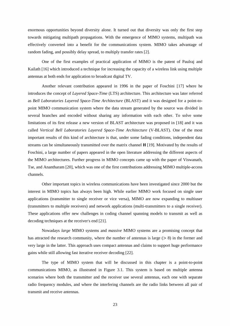
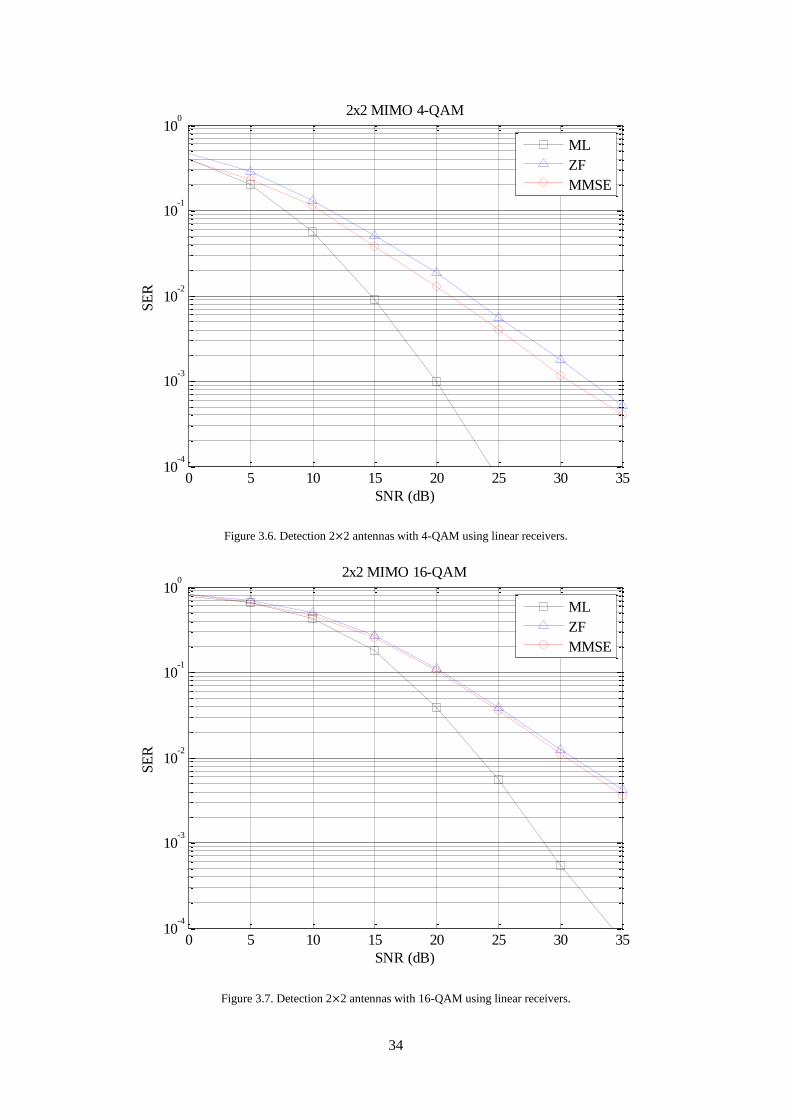
Figures 3.6 to 3.9 show the performance of ZF and MMSE linear receivers in different
configurations. The ML performance is also present as term of comparison with the best performance
attainable. Analysing the figures it possible observe that although MMSE receiver performs better
than the ZF both SER curves settle to a slope of -1 as proven in literature, which corresponds to a
decrease of symbol error rate by a factor of 10 for a 10-fold increase of SNR. From Figures 3.6 to 3.9
one can observe that MMSE detection has a power gain compared with ZF, i.e., it achieves the same
SER value from the 4-QAM constellation in a lower value of SNR, yet for higher constellations this
power gain decreases as well as for higher SNR values, becoming minimal.
Page 56
34
Figure 3.6. Detection 2 2 antennas with 4-QAM using linear receivers.
Figure 3.7. Detection 2 2 antennas with 16-QAM using linear receivers.
0 5 10 15 20 25 30 3510
-4
10-3
10-2
10-1
100
SNR (dB)
SE
R
2x2 MIMO 4-QAM
ML
ZF
MMSE
0 5 10 15 20 25 30 3510
-4
10-3
10-2
10-1
100
SNR (dB)
SE
R
2x2 MIMO 16-QAM
ML
ZF
MMSE
Page 57
35
Figure 3.8. Detection 3 3 antennas with 4-QAM using linear receivers.
Figure 3.9. Detection 3 3 antennas with 16-QAM using linear receivers.
0 5 10 15 20 25 30 3510
-5
10-4
10-3
10-2
10-1
100
SNR (dB)
SE
R
3x3 MIMO 4-QAM
ML
ZF
MMSE
0 5 10 15 20 25 30 35 4010
-5
10-4
10-3
10-2
10-1
100
SNR (dB)
SE
R
3x3 MIMO 16-QAM
ML
ZF
MMSE
Page 58
36
3.4 Order Successive Interference Cancellation Detection
Nonlinear methods on the receivers have to involve decision feedback somehow in order to
remove the interference between the signals from each antenna. In this context the most commonly
used approach is called order successive interference cancelation (OSIC). OSIC in fact corresponds
to the original algorithm proposed for the detection of the original V-BLAST transmission scheme in
[30]. As it was described in subsection 3.1, V-BLAST allows for the transmission of independent data
streams over the matrix channel .
While the transmission side of spatial multiplexing V-BLAST is straightforward, the
detection side is more difficult to implement since the signals from each antenna are received by all
the receive antennas. The principle of OSIC is to use linear detection to detect first the modulation
symbol of the layer least affected by noise and, subsequently, assuming that the first symbol was
correctly detected, the interference created by that symbol is replicated and subtracted from the others
layers. The procedure continues detecting the next best signal (again in the sense of the one with the
least noise enhancement) and subtracting the interference caused by it to the remaining layers, and
repeating this procedure until all symbols are detected.
The optimal criterion at each stage is to select the layer that less enhances the noise power
after the linear detection. It was shown in [29] that this corresponds to deciding for the layer that
spans the n-dimensional lattice by translating parallel hyperplanes of n-1 dimensions which have the
maximum separation among all possible families of hyperplanes. In doing this, the error probability is
minimised for that layer. This corresponds to ordered SIC, without which the performance of SIC is
seriously degraded by 3 dB[31].
Since the worst subchannel dominates the average SER this is the optimal criterion if all
subchannels use the same signalling rate and power. This result was already found in [30], in the first
implementation of the V-BLAST detector.
For a better understanding of the OSIC procedure let us follow a practical example of its
application on this work for 2 2 MIMO system through 4-QAM constellation and using ZF detection.
Consider the system of (3.1), where and
(3.20)
By applying the ZF linear transformations it is obtained
(3.21)
Page 59
37
(3.22)
The component of that experience the lowest noise enhancement by can be detected
with high reliability. Since ZMSW noise model is assumed this component corresponds to the row of
of smallest length, which is the Euclidean norm of the row.
(3.23)
By observation of (3.23) the lowest noise enhancement is associated with the first row, which
corresponds to the first antenna (layer). The next step is decide the symbol by quantization
(3.24)
Now the interference due to is replicated and then subtracted on the others layers
(3.25)
Once the symbol is already decided the first generator vector in the channel matrix
becomes zero. Thereby the matrix took into account to the second round of the algorithm is (3.26)
and its associated ZF linear transformation matrix (3.27).
(3.26)
(3.27)
Follows the calculation of the component of that experience the lowest noise but this time
over the estimates available via linear equalization of
(3.28)
At this stage the third row is the one that less enhances the noise and therefore is now
decided as
(3.29)
and its interference is subtracted from
Page 60
38
(3.30)
and the matrix H becomes in (3.31), where its third column is now null.
(3.31)
By applying the ZF linear transformations over it is obtained .
(3.32)
Finally remains estimate and the process comes to an end.
(3.33)
As expected all the symbols were correctly detected. However, one of the basic problems of
this strategy is that if one symbol is incorrectly detected, and for bad luck it is the first one to be
decided, it leads to a higher probability of wrongly detection to the following symbols.
Instead of ZF equalization it is also possible perform linear MMSE equalization to obtain a
MMSE version of the OSIC receiver. The only aspect that changes in what was exposed before is the
linear transformations should be replaced by the expression of MMSE equalization in the equation
(3.16).
The performance of OSIC receivers in different configurations can be found in Figures 3.10
to 3.13. In these figures are present both versions of OSIC receivers, the OSIC combined with ZF
(OSIC-ZF) and with MMSE (OSIC-MMSE) for 2 2 and 3 3 MIMO systems using 4 and 16 QAM
constellation. Moreover they can be compared with the ML detection. Although the performance of
the OSIC receiver capture the same diversity of ordinary linear receivers, by inspection of
Figures 3.6 to 3.9 one can conclude that it provides a large power gain when compared with the
ordinary linear receivers. Besides with the use of OSIC the MMSE equalizer performance presents a
higher difference of power gain to OSIC-ZF then the simple MMSE compared with the simple ZF.
One can conclude that the use of OSIC enhance more the performance of MMSE than ZF equalizer.
Page 61
39
Figure 3.10. Detection 2 2 antennas with 4-QAM using OSIC linear receivers.
Figure 3.11. Detection 2 2 antennas with 16-QAM using OSIC linear receivers.
0 5 10 15 20 25 30 3510
-5
10-4
10-3
10-2
10-1
100
SNR (dB)
SE
R
2x2 MIMO 4-QAM
ML
OSIC-ZF
OSIC-MMSE
0 5 10 15 20 25 30 3510
-5
10-4
10-3
10-2
10-1
100
SNR (dB)
SE
R
2x2 MIMO 16-QAM
ML
OSIC-ZF
OSIC-MMSE
Page 62
40
Figure 3.12. Detection 3 3 antennas with 4-QAM using OSIC linear receivers.
Figure 3.13. Detection 3 3 antennas with 16-QAM using OSIC linear receivers.
0 5 10 15 20 25 30 3510
-5
10-4
10-3
10-2
10-1
100
SNR (dB)
SE
R
3x3 MIMO 4-QAM
ML
OSIC-ZF
OSIC-MMSE
0 5 10 15 20 25 30 3510
-5
10-4
10-3
10-2
10-1
100
SNR (dB)
SE
R
3x3 MIMO 16-QAM
ML
OSIC-ZF
OSIC-MMSE
Page 63
41
3.5 Lattice Reduction-Aided Detection
The concept on lattice reduction-aided (LRA) detection arises naturally under this lattice
perspective. Considering the detection problem as a CVP, one wants to look for methods that produce
good approximate solutions (preferably, in polynomial time). The basic idea behind LRA is to use
lattice reduction in conjunction with traditional low-complexity decoders.
Using the lattice detection interpretation, given that the used constellations are QAM
constellations, and therefore , the noiseless received points in the communication
scenario corresponds to points of the lattice .
As was already discussed different bases can generate the same lattice, however there are
bases that perform linear equalizer (ZF and MMSE) decision regions which are closer to the ideal
Voronoi regions than others. Lattice reduction can be implemented by algorithms such as LLL and
KZ. These algorithms optimise the generating matrix of the lattice to obtain a “better” description of
the lattice [23]. The lattice points corresponds to integer linear combinations of the columns of
, and lattice reduction obtains another set of column vectors, collected in the reduced
matrix , which spans the same set of points, while having its generator vectors
more orthogonal to each other than the ones in the original basis. Since the matrix is composed
of more orthogonal vectors, the low-complexity detectors will perform better in this lattice because
the noise enhancement factor (which for example in linear equalisation amounts to ), is
decreased.
The matrices and are related by
(3.34)
where is a unimodular matrix, i.e., has integer entries and , therefore is also
unimodular and with integer entries.
Using equation (3.34) in (3.1) results in
(3.35)
and can be interpreted as the noiseless received signal points as the points in the lattice described by
. The original data vector can be recovered from nothing that
(3.36)
Page 64
42
The -QAM constellations used in this dissertation are defined without the origin and have
non unitary distance between the symbols. In order to apply lattice reduction algorithms it is
necessary to make a translation of the constellation, by creating the modified received vector
(3.37)
where p denotes a column vector of N elements all equal to 1.
After the lattice reduction pre-processing stage, any of receivers earlier described in this
dissertation may be used concatenated with the lattice reduction block, namely ZF, MMSE and OSIC.
The complex LLL (CLLL) was implemented in the simulations with LRA. Since the CLLL
reduces basis which are complex matrices, other components of MIMO detectors, such as the
computation of pseudo-inverse and QR decomposition, can also be operated with complex arithmetic
without doubling the channel matrix dimension. Thus, the use of CLLL helps reducing the complexity
of other parts of the MIMO detector, not just the reduction algorithm. CLLL directly operates on the
complex matrix , and because of that it only requires half of the complexity of traditional LLL using
the real equivalent model explained in subsection 3.3.1.
Table 4 represents the pseudo-algorithm implemented to simulate the LRA receivers.
Table 4 Pseudo-code of LRA detection.
1: Shift and scale the constellation to have zero as a lattice point:
2: Reduce the lattice basis H using CLLL:
3: Apply some detector to the CVP defined by
4: Using and estimate the symbol in the original coordinate system
Page 65
43
Figures 3.14 to 3.21 show the performance of LRA receivers in different configurations.
These configurations include 2 2 and 3 3 MIMO systems using both 4 and 16 QAM constellations.
The LRA receivers capture the same diversity of ML receivers as proved in literature. However they
suffer some power penalty. By analysing Figures 3.14 to 3.18 one can conclude that LRA ZF an LRA
MMSE in 2 2 MIMO system, taking into account the ML detection for each case, have less power
penalty when compared with its use in 3 3 MIMO system. Besides the power penalty difference
between LRA ZF and MMSE detection becomes higher in the 3 3 MIMO system, been the latter the
one that achieves better performance losing only a few dB from the optimal ML detection in 2 2
MIMO system. In the lattice reduction followed by OSIC strategies, depicted in Figures 3.19 to 3.21,
it is possible to observe that the power gain over the LRA linear receivers is large, specially for the
case of 3 3 MIMO system. Furthermore the fact observed in section 3.4 is also noticed, once that
after the pre-processing stage of lattice reduction the OSIC-MMSE performs much better than the
OSIC-ZF detection. For a 2 2 MIMO system using 4-QAM constellation, the LRA OSIC-MMSE
receivers have less than 1 dB of power penalty (see Figure 3.18).
Reviewing all the strategies implemented for the MIMO detection the performance results
points to the conclusion that LRA OSIC-MMSE receiver is the one that achieves the best
performance. It capture the same diversity order of ML detection, , and among the other
receivers is the one that has the smaller power penalty compared with ML. On the other hand is also
the one that needs more computation, so apart from the LRA receivers is OSIC-MMSE receiver
whose has the best performance. It has a slope of -1 but is the one that minimizes the power penalty
compared with ML detection, again apart from LRA receivers.
Page 66
44
Figure 3.14. Detection 2 2 antennas with 4-QAM using LRA linear receivers.
Figure 3.15. Detection 2 2 antennas with 16-QAM using LRA linear receivers.
0 5 10 15 20 25 3010
-5
10-4
10-3
10-2
10-1
100
SNR (dB)
SE
R
2x2 MIMO 4-QAM
ML
LRA ZF
LRA MMSE
0 5 10 15 20 25 30 3510
-5
10-4
10-3
10-2
10-1
100
SNR (dB)
SE
R
2x2 MIMO 16-QAM
ML
LRA ZF
LRA MMSE
Page 67
45
Figure 3.16. Detection 3 3 antennas with 4-QAM using LRA linear receivers.
Figure 3.17. Detection 3 3 antennas with 16-QAM using LRA linear receivers.
0 5 10 15 20 25 30 3510
-5
10-4
10-3
10-2
10-1
100
SNR (dB)
SE
R
3x3 MIMO 4-QAM
ML
LRA ZF
LRA MMSE
0 5 10 15 20 25 30 3510
-5
10-4
10-3
10-2
10-1
100
SNR (dB)
SE
R
3x3 MIMO 16-QAM
ML
LRA ZF
LRA MMSE
Page 68
46
Figure 3.18. Detection 2 2 antennas with 4-QAM using LRA OSIC linear receivers.
Figure 3.19. Detection 2 2 antennas with 16-QAM using LRA OSIC linear receivers.
0 5 10 15 20 25 3010
-5
10-4
10-3
10-2
10-1
100
SNR (dB)
SE
R
2x2 MIMO 4-QAM
ML
LRA OSIC-ZF
LRA OSIC-MMSE
0 5 10 15 20 25 30 3510
-5
10-4
10-3
10-2
10-1
100
SNR (dB)
SE
R
2x2 MIMO 16-QAM
ML
LRA OSIC-ZF
LRA OSIC-MMSE
Page 69
47
Figure 3.20. Detection 3 3 antennas with 4-QAM using LRA OSIC linear receivers.
Figure 3.21. Detection 3 3 antennas with 16-QAM using LRA OSIC linear receivers.
0 5 10 15 20 25 30 3510
-5
10-4
10-3
10-2
10-1
100
SNR (dB)
SE
R
3x3 MIMO 4-QAM
ML
LRA OSIC-ZF
LRA OSIC-MMSE
0 5 10 15 20 25 30 3510
-5
10-4
10-3
10-2
10-1
100
SNR (dB)
SE
R
3x3 MIMO 16-QAM
ML
LRA OSIC-ZF
LRA OSIC-MMSE
Page 71
49
Chapter 4
MIMO combined
with PLNC
The present chapter proposes a set of new strategies
combining MIMO with PLNC in scenarios that
move beyond the traditional TWRC.
4 MIMO combined with PLNC
Page 72
50
4.1 System Model
Chapter 3 introduced the concept of MIMO systems as well as the most part of the strategies
used to solve the CVP. Using these MIMO techniques in a context involving PLNC is the objective of
this chapter. One suitable name for the following described scenarios may be PLNC in a network with
a MIMO relay. Different communication strategies and different scenario configurations will be
considered.
The main idea of PLNC exploited in this dissertation is to create a mechanism similar to
network coding, however implemented at the very bottom of the physical layer that deals with EM
signal reception and modulation. Through a proper modulation and demodulation technique at the
nodes additions of EM signals can be properly defined, so that the interference becomes part of the
arithmetic operation of the network coding.
Understanding the structure of the physical layer is of utmost importance for the proposals
that will be presented in this chapter. The physical layer considered in this dissertation is the wireless
medium and thus its properties will be reviewed, despite the fact that some of them have already been
considered implicitly in the previous chapter. Based on [10] in a PLNC perspective there are three key
observations to be made:
1) Signal fading is linear:
Between the transmitter and a receiver, an EM signal experiences a linear
transformation. This transformation is primarily caused by reflections and multipath
propagation. Assuming band-limited communication the respective signals can be
represented uniquely by complex-valued discrete-time samples. Then the received signal
at any point in space can be expressed as the convulsion of the transmitted signal with an
impulse-response function that characterizes the signal propagation. So a usual approach
is to model this impulse response function in a statistical way instead of modeling exactly
the physical surroundings.
Assuming flat (i.e., frequency non-selective) fading, as it would be appropriate for
narrow band communication, this impulse response function reduces to a delayed Dirac
delta function whose height and time-delay characterizes the signal. This time delay may
be viewed as a phase-shift in the discrete-time simulation model. This particularly simple
model is the one considered in the previous chapter and is now applied to a network.
Taking into account the concept of time-slot, the induced signal can be expressed as
where is the sequence of complex symbols transmitted at the symbol transmission
period . The prevalent model in the literature assumes a random fading taken from a
zero-mean circularly symmetric complex Gaussian distribution with unit variance, as it
Page 73
51
was also considered in Chapter 3. As well as in the previous chapter the strategies
discussed below require CSIR, which is motivated by signal measurements that can be
acquired at the receiver. Notice that the transmitter is oblivious to .
2) Multiple signals interfere in a linear additive way:
Instead of considering one transmitter only, let us now consider nodes transmitting
simultaneously. According to observation 1, the induced signal at any point in space can
be expressed as
(4.1)
It is commonly assumed that the respective fading coefficients are independent
from each other since each node transmits from a different position in space. Throughout
this chapter all those coefficients follow also a zero-mean circularly symmetric complex
Gaussian distribution with unit variance and, in order to have an independent and
identically distributed Rayleigh fading channel model, the phase of each is uniformly
distributed in , and its amplitude has a Rayleigh distribution (cf. chapter 3).
3) Noise is independent of the signal and added at the receiver:
At any receiving antenna one has to consider some additive noise, denoted by
which is taken from an independent circularly symmetric complex Gaussian with zero
average and variance corresponding, usually dubbed as the ZMSW noise model.
Taking into account these three observations along with several other detailed considerations
[31] it is possible to define the commonly used model for the signal at a particular receiver when
multiple nodes are simultaneously transmitting as
(4.2)
Notice that the errors caused by the noise always accumulate over the various stages of the
network, which is an undesirable element for linear network coding at the physical layer.
In order to better explain the model implemented other detailed considerations have to be
made, especially for the understanding of the matched filter. As previously mentioned, this model
works with the complex baseband representation of discrete time signals. Figure 4.1 shows the
communication system diagram assumed in this dissertation and Figure 4.2 the full system diagram in
continuous time.
Page 74
52
Figure 4.1. Simplified system diagram in discrete-time.
Figure 4.2. Full system diagram in continuous-time.
In Figure 4.2 the real and imaginary components of are sequences of pulse amplitudes,
which are each passed through a transmit filter . The filtered signals are then modulated, giving rise
to both in-phase and quadrature components transmitted over the channel by the carrier. The channel
is modelled as a linear filter and the Gaussian noise, , is added at the receiver, as considered
in observation 3). Note that the modulation and demodulation stages are not represented in the
figures. After demodulation, the base-band signal is passed through a receiver filter and then
sampled for further discrete-time processing. Assuming that the samples are taken at the optimal
detection instant, the discrete-time channel impulse response may equivalently be defined by the
convolution (denoted by the symbol “ ”), as shown for example in [32],
(4.3)
In the conventional communications approach, the receive filter is matched to the
convolution of the transmitted pulse and the channel impulse response , i.e.,
while the matched filter is defined as
(4.5)
where denotes some real gain and is the conjugate of [32]. This matched filter weights
the received signal according to the signal amplitude and also aligns its phase to maximize the output
SNR [2] and this maximises the SNR at some optimal sampling instant. The signal then becomes
(4.6)
(4.4)
Transmit
filter
Receiver
filter Detector Decision
device
Channel
Decision
device Detector
Channel
Page 75
53
and therefore (see Figure 4.1) can be obtained as,
(4.7)
Using this matched filter, which, when generalised to the detection of vector messages, is
known as the maximal ratio combiner, the effects of the channel are typically compensated. In the
discrete-time domain this can be interpreted as applying a normalized detection filter [32],
(4.8)
In short, the estimate obtained by the matched filter can be represented as,
. (4.9)
Notice that the compensation of the effects of the channel performed by this matched filter is
different to the ones achieved by , which was introduced in section 3.3. This is because the
matched filter cannot deal with interference, treating everything as noise. On the other hand, zero
forcing focuses on removing the interference only and then considers noise. The matched filter can
only be used when only one message is expected to exist in the signal, cleared from all other
interference coming from other users or antennas, which is seldom the case in the systems tested in
this work. Notice too that should be denoted by , however, given that in the remainder of this
dissertation only slow fading channels are considered, meaning that they stay constant over many
transmitted symbols, these coefficients were simply denoted by .
Perfect synchronization between the nodes is assumed in this dissertation, however,
synchronization is for long time an active research problem in wireless networks. Symbol time and
carrier-frequency synchronizations, which are both needed in PLNC, have been actively investigated
by researchers in fields such as OFDMA [33].
There are three areas of PLNC research: communication-theoretic, information-theoretic and
networking aspects, out of which, networking has received the least attention. Nevertheless, this issue
becomes even more important when we extend the application of PLNC beyond TWRC. PLNC in
TWRC have been intensively researched in the recent PhD dissertation [34], where a strategy
exploring the intersection of PLNC, MIMO, and the Alamouti coding scheme are proposed. However,
that research did not venture beyond the TWRC. As soon as the theoretical understanding of this
scenario matures, it is most likely that the research focus will move towards the application of PLNC
to general topologies. Up until now, the literature on this area is scarce and it is difficult to find
examples to compare with.
Page 76
54
The goal of this chapter is to propose some strategies to implement PLNC beyond TWRC,
while including MIMO links and detection strategies. Notwithstanding a first attempt to combine
PLNC with MIMO will be start with the TWRC. More specifically, the assumed scenario consists of a
certain number of terminals that want to exchange messages among them, while knowing that there is
no direct link between them. Therefore they have to revert to a communication made through a relay.
All the nodes are considerer half duplex, i.e., they do not transmit and receive at the same time.
In all the strategies proposed, the uplink (from the terminals to the relay) consists of
decentralized transmitters (mobile terminals) and, on a first iteration of the communication protocol, a
central receiver (MIMO relay), which in the following phase becomes a central transmitter.
Considering terminals equipped with a single antenna and a relay equipped with a number of antennas
equal to the number of terminals, it can be considered as a distributed MIMO system (multipoint-to-
point). The uplink direction of any multiuser mobile communication system is an example of a
distributed MIMO system. The role of the base station is to recover the individual users’ signals from
its received signal, and because a number of users transmit at the same time in the same band, this
received signal is the superposition of all the active users’ signals [23]. Figure 4.3 illustrates the
scenario considered in the uplink.
Figure 4.3. Distributed MIMO at the uplink phase.
Given that the uplink scenario is a MIMO system, although it is a distributed one, all the
detection strategies discussed in Chapter 3 can be applied.
The MIMO relay receives the sum of the signals coming from the different terminals and
detects the message sent by each user. Then, in the downlink, it chooses a strategy to send the
messages back to the terminals in order to succeed the exchange of messages between them. After
receiving the sum of the signals sent by the MIMO relay each terminal attempts to obtain the
Relay
Terminals
Page 77
55
messages from the other terminals. Very importantly, in this dissertation all channels are considered
reciprocal, i.e., they are the same for the uplink and downlink phase.
The strategies used at the receivers in the downlink are based in a PLNC perspective since
they take advantage of the fact that propagation in wireless medium results in a signal that is a linear
combination of the signals sent by the MIMO relay, i.e., the receivers know which are those linear
combinations once it is considered CISR and so they can cancel the channel effect. However the
decoding results may not be precise due to the induced noise (see equation (4.2)).
Furthermore the signal that each terminal receives in the downlink contains, in the majority of
cases discussed, the message that the terminal itself sent in the uplink phase. Consequently each
terminal can subtract the contribution of its message from the downlink received signal, what can be
seen as self interference cancelation. Then each terminal tries to decode the messages from the other
ones using this “reduced” signal, performing a detection strategy that will be described later on for
each specific scenario.
Besides the traditional TWRC configuration, this dissertation proposes to combine MIMO
techniques with PLNC in a scenario with three users and a relay. While in the TWRC case the
traditional scheme takes 4 time-slots to accomplish the exchange of messages, as it was explained in
Chapter 1, it is straightforward to intuit that in the new scenario, with three terminals and a relay, the
permutation of the messages takes 6 time-slots.
There will be considered two strategies for the exchange of messages in the scenario with
three terminals: one that uses just 2 time-slots, improving the throughput in 150%, and another one
that uses 3 time-slots, which have an improvement of 100% compared to the traditional scheme.
For all the cases discussed, one can assume that the MIMO relay has a high processing
capacity and because of that the uplink will always use LRA OSIC-MMSE detection and the uplink
takes just one time-slot making use of the distributed MIMO system. This option was taken because
LRA OSIC-MMSE was the detection strategy that achieved the best performance among the others in
the previous chapter, excluding ML detection that has exponential time consumption.
The SER of the downlink phase it is obtained comparing the messages decoded by each
terminal with the original messages sent by them in the uplink phase. Notice that the downlink
performance suffers from errors due to the previous uplink detection in the relay. This reinforces the
choice of LRA OSIC-MMSE in the MIMO relay as an attempt to minimize the impact in downlink
performance.
As it was stated in Chapter 3 the newly implemented strategies performance results will be
plotted as symbol error rate (SER) as function of the SNR defined in (3.4) and both terminals and
Page 78
56
relay will make use of the same -QAM constellations. Notice that for simplicity of results the plots
will just have one curve for the uplink, regarding the MIMO relay, and another one for the downlink
representing just one terminal since the others will present a quite similar performance.
The following section will present in detail the detections methods implemented at the
downlink for the TWRC and for the three terminals with a relay scenario. As was already mentioned
the latter will be divided in the two time-slot and three time-slot approaches. One last strategy
presented is a two time-slot strategy where the terminals are MIMO terminal equipped with two
antennas.
4.2 MIMO combined with PLNC in TWRC
The MIMO combined with PLNC in TWRC strategy is illustrated in Figure 4.4 and Figure
4.5. The two terminals are equipped with a single antenna and the relay with two antennas. The
channel coefficients are also depicted in both Figures and the messages exchanged are denoted by
.
Figure 4.4. Uplink phase on MIMO combined with PLNC in TWRC.
Figure 4.5. Downlink phase on MIMO combined with PLNC in TWRC.
In the uplink terminals 1 and 2 send their messages to the relay. As in an ordinary 2 2
distributed MIMO system the relay receives the messages (from terminal 1) and (from terminal
2). Then the relay sends in one antenna and in the other one. This transmitting configuration is
1
2
1
2
h11
h12
h21h22
x1
x2
Relay
Relay
1
2
1
2
h11
h12
h21h22
x1
x2
Page 79
57
assumed to be known in advance by the terminals and therefore, accordingly with what was described
in section 4.1, the received signal, for example, of terminal 1 is given by
(4.10)
The terminal possesses channel state information (CSIR) and knows its own sent uplink
message. Hence the first step of the decoding process amounts to canceling its own contribution from
the received signal, resulting in
(4.11)
Making use of a simple matched filter that cancels the channel linear transformation
experienced by message , terminal 1 can obtain a noisy version of the message and then apply a
quantization step,
(4.12)
The aforementioned procedure is followed by terminal 2 in an equivalent way. The
performance of this strategy is presented hereafter in Figures 4.6 and 4.7 for the 4 and 16-QAM
constellations, respectively, recalling that uplink performance is achieved by a LRA OSIC-MMSE
receiver. The performance results of this strategy are lower than the ones presented in [34] for TWRC,
since here Alamouti coding scheme was not used. However the throughput of the present strategy is
improved by 100% compared with the traditional scheme as it was discussed in Chapter 1, obtaining a
reduction of communications from 6 time-slots to 2 time-slots.
Page 80
58
Figure 4.6. Detection MIMO combined with PLNC in TWRC using 4-QAM.
Figure 4.7. Detection MIMO combined with PLNC in TWRC using 16-QAM.
0 5 10 15 20 25 30 3510
-5
10-4
10-3
10-2
10-1
100
SNR (dB)
SE
R
4-QAM
Uplink
Downlink
0 5 10 15 20 25 30 3510
-5
10-4
10-3
10-2
10-1
100
SNR (dB)
SE
R
4-QAM
Uplink
Downlink
Page 81
59
4.3 PLNC in a Network with a MIMO Relay
The scenario assumed in the following subsections consists of three terminals which aim to
exchange messages between them. The messages are symbols , where the index refers to the
terminal from where the symbol was originally transmitted in the uplink. There is a direct link
between the terminals and the relay, which means that the terminals do not receive any signal from
other terminals and can only communicate through the relay. The uplink consists of a simple case of a
distributed 3×3 MIMO system with a relay equipped with three antennas while the terminals only use
one antenna to transmit their messages to the relay. This stage takes only one time-slot and the MIMO
relay makes use of a LRA OSIC-MMSE receiver to decode the messages sent by the terminals. The
uplink phase is equal for all the strategies discussed along this section, and therefore only the different
downlink phases will be presented in the following sub-sections. Figure 4.8 illustrates the uplink
phase and the channel coefficients considered.
Figure 4.8. Uplink phase with 3 terminals.
4.3.1 Two Time-slots Strategy
In the uplink the MIMO relay decodes the messages and coming from the three
terminals. In the two time-slots strategy the downlink phase, depicted in Figure 4.9, consists in the
transmission of those messages where each antenna of the relay transmits one of the received
messages, i.e., antenna 1 of the relay transmits , antenna 2 transmits and antenna 3 transmits ,
all at the same time in the second time-slot.
1
2
1
2
h11
h12
h22
x1
x2
Relay
3x3
3
h13
h33
h21
h23
h32
h31
Page 82
60
Figure 4.9. Downlink phase on two time-slot strategy with 3 terminals.
The above-mentioned transmitting configuration is assumed to be known in advance by the
terminals and therefore, after the linear transformation performed by the wireless medium described
in section 4.1, the received signal at each terminal is given by
(4.13)
(4.14)
(4.15)
The coefficients are the ones represented in Figure 4.9 and denote the received signal at
the terminal. Since all terminals possess CSIR and knows its own sent uplink message, the first
step of the decoding process amounts to canceling its own contribution from the received signal,
resulting in
(4.16)
(4.17)
(4.18)
The obtained are now decoded making use of brute force (ML) detection discussed in
section 3.2 allowing each terminal to estimate the other two messages. In this first configuration, it is
very important to note that this ML detection is made using the projections of the signals in just one
dimension, since the are just a scalar and not vectors, as in section 3.2. Therefore, signal detection
will be much affected by noise given that in this projective space the Euclidean distance between
symbols is not lower bounded which eventually contributes in a decisive way to the poor performance
1
2
1
2
h11
h12
h22
x1
x2
Relay
3 x33
h13
h33
h21
h23
h32
h31
Page 83
61
of this strategy. It is also worth pointing out that the downlink performance suffers from errors due to
the previous uplink detection in the relay.
This strategy was simulated for 4 and 16-QAM modulation and the performance results are
presented in Figures 4.10 and 4.11. One can conclude that the performance of such strategy, apart
from the higher complexity due to ML detection, is lower than the one obtained in MIMO combined
with PLNC in TWRC case, even though it concerns three terminals. Nevertheless, the throughput of
the present strategy is improved by 150% compared with the traditional scheme, reducing the
communications from 6 time-slots to 2 time-slots.
Page 84
62
Figure 4.10. Detection two time-slot strategy with 3 terminals using 4-QAM.
Figure 4.11. Detection two time-slot strategy with 3 terminals using 16-QAM.
0 5 10 15 20 25 30 3510
-4
10-3
10-2
10-1
100
SNR (dB)
SE
R
4-QAM
Uplink
Downlink
0 5 10 15 20 25 30 3510
-4
10-3
10-2
10-1
100
SNR (dB)
SE
R
16-QAM
Uplink
Downlink
Page 85
63
4.3.2 Three Time-slots Strategy
Considering the scenario described for these sub-sections in the uplink the MIMO relay
decodes the messages and in one time-slot. This three time-slot strategy uses 2 time-slots in
the downlink phase, as illustrated in Figures 4.12 and 4.13. So in the second time-slot, which
corresponds to the first one in the downlink phase, the relay transmits the messages and on
antenna 1 and 2, respectively.
Figure 4.12. First time-slot from downlink phase on three time-slot strategy with 3 terminals.
Figure 4.13. Second time-slot from downlink phase on three time-slot strategy with 3 terminals.
The above-mentioned transmitting configuration and the one considered for the second time-
slot of the downlink phase are assumed to be known in advance by the terminals and therefore, taking
into account the model described in section 4.1, the received signal at each terminal at the first time-
slot of the downlink phase is given by
(4.19)
(4.20)
1
2
1
2
h11
h12
h22
x1
x2
Relay
33
h13
h21
h23
1
2
1
2
h11
h12
x1
3 x33
h13
h33
h32
h31
Relay
Page 86
64
(4.21)
where the coefficients are the ones represented in Figure 4.12 and denote the received signal at
the terminal at the time-slot . Notice that each terminal possesses CSIR.
At this point both terminal 1 and 2 know that they are receiving a signal that contains the
message that they sent in the uplink phase so the first step of the decoding process amounts to
canceling its own contribution from the received signal, resulting in
(4.22)
(4.23)
and making use of simple matched filter terminal 1 estimates from (4.24) and terminal 2 estimates
from (4.25).
(4.24)
(4.25)
Terminal 3 saves the received signal in order to process it later. Resuming after the first time-
slot of the downlink phase terminal 1 have and terminal 2 have while terminal 3 have the
information in (4.21).
In the third time-slot, time-slot 2 of downlink (see Figure 4.13), the relay transmits the
messages and on antenna 1 and 3, respectively, and the signals received by the terminals are
(4.26)
(4.27)
(4.28)
By now terminal 1 and 3 know that they are receiving their uplink original messages whereas
terminal 2 can use its estimated . Therefore next step amounts to canceling each one of these
contribution from the received signal at each terminal, resulting in
(4.29)
(4.30)
Page 87
65
(4.31)
and again using a simple matched filter both terminal 1 and 2 estimate from (4.32) and (4.33),
respectively, and terminal 3 estimates from (4.34).
(4.32)
(4.33)
(4.34)
Terminal 1 and 2 have now all the messages. Finally, using the information in (4.21), terminal
3 can compute (4.35) and apply a simple matched filter in order to estimate from (4.36).
(4.35)
(4.36)
This strategy was also simulated for 4 and 16-QAM modulation and the results are presented
in Figures 4.14 and 4.15. One can conclude that the performance of such strategy accomplishes better
results than the approach using just two time-slots described in subsection 4.3.1. Furthermore is
clearly less complex than the previous one since only simple computation processes and simple
matched filters are applied. However this strategy loses 50% of throughput improvement when
compared with the two time-slot strategy but it still achieves a throughput improvement of 100%
when compared with the traditional scheme, reducing the communication from 6 time-slots to 3 time-
slots.
Page 88
66
Figure 4.14. Detection three time-slots strategy with 3 terminals using 4-QAM.
Figure 4.15 Detection three time-slot strategy with 3 terminals using 16-QAM.
0 5 10 15 20 25 30 3510
-4
10-3
10-2
10-1
100
SNR (dB)
SE
R
4-QAM
Uplink
Downlink
0 5 10 15 20 25 30 3510
-4
10-3
10-2
10-1
100
SNR (dB)
SE
R
16-QAM
Uplink
Downlink
Page 89
67
4.3.3 Two Time-slots Strategy with MIMO Terminals
The high SER obtained on the strategy discussed in subsection 4.3.1 is explained mostly by the
lost of dimensions in the downlink since ML detection is made using the projections of the signals in
just one dimension as it was explained. Besides the use of brute force ML detection increases
complexity at the terminals so in the present sub-section a new version of that strategy is proposed.
The goal is to maintain the throughput improvement of 150% over the traditional scheme, gain
performance and reduce complexity in the detection process taking advantage from a new dimension.
The scenario considered for the uplink stays the one specified for section 4.3.
In order to attain this new dimension the two time-slots strategy with MIMO users assumes that
terminals are now equipped with two antennas instead of a single one. The uplink remains as it was
considered (see Figure 4.8) for all the strategies discussed in this section, so the users transmit their
messages at the same time-slot using a single antenna as previously stated.
Figure 4.16. Downlink phase on two time-slot strategy with 3 MIMO terminals.
The reception on the downlink phase makes use of the two antennas of the terminals. Since the
process of the detection will be the same for the three terminals it will only be reproduced the
procedure example concerning reception on terminal 1 (see Figure 4.16).
MIMO relay decodes the uplink messages and then each antenna of the relay
transmits one of the received messages, i.e., antenna transmit , all at the same time in the second
time-slot. The transmitting configuration is assumed to be known in advance by the terminals and
therefore the sum of the received signal at the two antennas of each terminal, in this example just
terminal 1, is given by
(4.37)
(4.38)
1
2
1
2
h11
h21
h22
x1
x2
Relay
3 x33
h31
h12
h32
1
2
Page 90
68
The coefficients are the ones represented in Figure 4.16 and denote the received signal
at the terminal and its antenna. Since the terminal possesses CSIR and knows what was its own
sent uplink message the first step of the decoding process amounts to canceling its own contribution
from the received signal, resulting in
(4.39)
(4.40)
After calculate this self interference cancelation the system can be rewritten as (4.41) or
equivalently (4.42).
, (4.41)
(4.42)
Therefore accordingly with the model described in section 4.1 this system is equivalent to the
one described in equation (3.1), once that the system model of Chapter 3 is also valid for the present
chapter which means that the system of (4.42) can be interpreted as a MIMO communications of
antennas. Consequently all the detections strategies considered along Chapter 3 can be
applied.
Summarizing in the two time-slots strategy with MIMO terminals each one of them exploits
the linear codification induced by the wireless medium to reduce the detection problem to a
2 2MIMO equivalent system and then apply a detection strategy decoding the messages from the
other two terminals. This strategy is simulated for 4 and 16-QAM modulation. As expected the
performance of this scheme brings down the SER curve especially for the LRA decoders. Depending
on the computation capacity of the terminals it can be chosen an appropriate decoding strategy
requiring more or less computation and consequently more or less energy consumption. Within this
perspective it will be presented the performances for OSIC-MMSE (see Figures 4.17 and 4.18) and
LRA OSIC MMSE (see Figures 4.19 and 4.20) decoders once they are the ones that achieve a better
performance and have a substantial difference of computation. Concluding PLNC combined with a
MIMO relay and MIMO users guarantees the best performance of the scenario described in section
4.3, ensuring a polynomial computational time and having a throughput improvement of 150%
competing with the traditional scheme. This strategy can be generalized for scenarios with
terminals equipped with antennas and a MIMO relay equipped with antennas. For instance in
a scenario with four terminals the throughput improvement raises up to 200% competing with the
traditional scheme, reducing the communication from 8 time-slots to 2 time-slots.
Page 91
69
Figure 4.17. OSIC-MMSE using 4-QAM in two time-slot strategy with MIMO terminals.
Figure 4.18. OSIC-MMSE using 16-QAM in two time-slot strategy with MIMO terminals.
0 5 10 15 20 25 3010
-5
10-4
10-3
10-2
10-1
100
SNR (dB)
SE
R
4-QAM
Uplink
Downlink
0 5 10 15 20 25 3010
-5
10-4
10-3
10-2
10-1
100
SNR (dB)
SE
R
16-QAM
Uplink
Downlink
Page 92
70
Figure 4.19. LRA OSIC-MMSE using 4-QAM in two time-slot strategy with MIMO terminals.
Figure 4.20. LRA OSIC-MMSE using 16-QAM in two time-slot strategy with MIMO terminals.
0 5 10 15 20 25 30 3510
-4
10-3
10-2
10-1
100
SNR (dB)
SE
R
4-QAM
Uplink
Downlink
0 5 10 15 20 25 30 3510
-4
10-3
10-2
10-1
100
SNR (dB)
SE
R
16-QAM
Uplink
Downlink
Page 93
71
Chapter 5
Conclusions
The present chapter points to the conclusions of the
dissertation and describes possible future directions
for the work developed.
5 Conclusions
Page 94
72
5.1 Main Conclusions
This thesis chiefly deals with the concept of interference cancellation when a receiver knows
the channel that each of the interfering messages have gone through. This may be the case in “pure”
MIMO, or when merging the concept of successive interference cancelation (SIC) with physical layer
network coding, interpreting PLNC as a first stage of SIC.
In this dissertation lattices (described in Chapter 2) have a prominent role given that their
structure is closely related to the MIMO detection problem, which has been a central research topic in
MIMO communication in the last decade. From a lattice perspective, MIMO detection is known as the
closest vector problem (CVP), as described in Chapter 3. In this chapter, several suboptimal solutions
addressing this problem have also been described. Taking into account the detection techniques
implemented for MIMO, the performance results point to the conclusion that although LRA receivers
capture the same diversity order of ML detection, , the LRA OSIC-MMSE receiver is the one
that achieves the best performance since it is the one that has the smaller power penalty compared to
the optimal ML detection. In some configurations the power penalty in respect to ML is reduced
approximately to 1 dB only. It is remarkable that LRA OSIC-MMSE achieves this performance in
polynomial time instead of the exponential performed by ML (which is chiefly due to the polynomial
complexity of the celebrated LLL algorithm). On the other hand, excluding ML detection, this
receiver is the one that needs more computation. However, it is important to notice that most of the
complexity is not associated with the detection of each symbol vector but rather associated with the
reduction of each matrix representing a channel. Consequently, the lattice reduction algorithm is only
needed to be computed when the channel changes, which for slow fading channels is sparsely need.
Apart from LRA receivers, the OSIC-MMSE receiver has the best performance since it is the one that
minimizes the power penalty in comparison to ML detection. In general, ZF, MMSE, and OSIC
receivers all have the same diversity order ( ) but OSIC receivers present a larger gain than the
others. The performance gain from ZF to MMSE is small and tends to decrease with a higher number
of antennas and higher-order -QAM constellations. The implementation of complex-LLL not only
reduces the complexity of the lattice reduction algorithm, but also achieves that without sacrificing
any performance when compared with traditional real-valued LLL. Additionally, it also helps to
reduce the complexity of other parts of the MIMO receivers involving matrix computations.
Chapter 4 puts in practice the concepts of PLNC (introduced in Chapter 1) and proposes a set
of new strategies combining MIMO with PLNC in scenarios that move beyond the traditional TWRC.
One should notice that in all these strategies, the uplink is actually a distributed MIMO system and in
the downlink we looked at three different approaches, all of which make use of some sort of self-
interference cancelation. The two time-slots strategy proved to have the lowest performance, which
can be explained by the fact that ML detection is implemented using the projections of the signals in
Page 95
73
just one dimension rather than deciding for symbols in a multi-dimensional lattice. Since ML
detection is used, this strategy has exponential complexity; however, it has a 150% capacity increase
in respect to traditional TDMA. The three time-slots strategy exceeds the performance of the two
time-slots strategy and is clearly less complex because it only involves a simple cancelation of terms
and a matched filter. This latter strategy achieves a 100% throughput improvement compared with the
traditional scheme, but nevertheless it loses 50% of throughput improvement when compared with the
previous one. Finally the two time-slots strategy with MIMO terminals is the most attractive. It
provides a 150% improvement in respect to the traditional scheme and does it using simple
computation processes in a first step and then can perform any of the suboptimal solutions found on
Chapter 3. The superior performance achieved by this strategy is obtained using LRA OSIC-MMSE
receivers in all terminals and also at the relay. One should note that this strategy can always be
generalized to scenarios with terminals, each of which equipped with antennas and the
MIMO relay equipped with antennas, allowing the exchange of messages in just two time-slots.
5.2 Future Work
A natural next step for this research is to implement the two time-slots strategy with MIMO
terminals in scenarios with more than three terminals and demonstrate the generalization above
mentioned to terminals. A more elaborate extension would be implementing full-duplex nodes, i.e.,
nodes that transmit and receive at the same time in the same frequency band, combined with PLNC
and MIMO techniques. In full-duplex configurations the detection processes need not only to consider
the interference coming from other special streams or from other terminals, but self-interference needs
also to be taken into account.
The properties of lattices made them central in the other branch of PLNC, which is the
Compute and Forward approach, as introduced in Chapter 1 and that should probably become the
main road to be explored in PLNC for instance by forcing an isomorphism between the lattice
structure and group codes with worlds associated with lattice points, meaning that the sum of any two
codewords always give rise to another valid codeword.
Page 97
75
References
[1] F. Boccardi, B. Clerckx, A. Ghosh, E. Hardouin, G. Jöngren, K. Kusume, E. N. Onggosanusi
and Y. Tang, “Multiple-antenna techniques in LTE-advanced,” IEEE Commun. Magazine, vol.
50, no.2, pp. 114-121, February 2012.
[2] D. Tse and P. Viswanath, “Fundamentals of Wireless Communication,” Cambridge University
Press, New York, USA, 2005.
[3] S. Zhang, S. C. Liew, P. P. Lam, “Hot Topic: Physical-layer Network Coding,” ACM
MobiCom’06, pp. 358-365, September 2006.
[4] P. Popovski and H. Yomo, “The anti-packets can increase the achievable throughput of a
wireless multi-hop network,” in Proc. of IEEE Int. Conf. on Commun., Istanbul, Turkey, pp.
3885–3890, June 2006.
[5] B. Nazer and M. Gastpar, “Computing over multiple-access channels with connections to
wireless network coding,” in Proc. of IEEE Int. Symp. on Inf. Theory, Seattle, USA, pp. 1354–
1358, July 2006.
[6] Y. Wu, P. A. Chou, and S.-Y. Kung, “Information exchange in wireless networks with network
coding and physical-layer broadcast,” Microsoft Research, Redmond, WA, Tech. Rep. MSR-
TR-2004-78, August 2004.
[7] C. Feng, D. Silva and F. R. Kschischang, "An algebraic approach to physical layer network
coding," in Proc. of ISIT'10 – The Inter. Symp. on Information Theory, Austin, TX, USA, pp.
1017-1021, June 2010.
[8] S. C. Liew, S. Zhang and L. Lu, “Physical-layer network coding: Tutorial, survey, and beyond,”
Physical Communication, vol. 6, pp. 4–42, March 2013.
[9] B. Nazer and M. Gastpar, “Compute-and-Forward: Harnessing Interference through Structured
Codes,” IEEE Trans. Info. Theory, to appear, June 2011.
[10] B. Nazer and M. Gastpar, “Reliable Physical Layer Network Coding,” Proceedings of the IEEE,
vol. 99, no. 3, March 2011.
[11] B. Nazer and M. Gastpar, “Compute-and-forward: A novel strategy for cooperative networks,”
42nd Asilomar Conference on Signals, Systems and Computers, October 2008.
[12] O. Revev, lecture notes, "Lattices in Computer Science," Tel Aviv University, Fall 2009,
http://www.cims.nyu.edu/~regev/teaching/lattices_fall_2009/.
Page 98
76
[13] D. Micciancio, “Lattices Algorithms and Applications,” University of California, San Diego,
Winter 2010.
[14] A. K. Lenstra, H. W. Lenstra, Jr., and L. Lovász, “Factoring polynomials with rational
coefficients”, Math. Ann. vol. 261, no.4, pp. 515–534, 1982.
[15] X. Ma and W. Zhang, “Performance analysis for MIMO systems with lattice-reduction aided
linear equalization,” IEEE Transactions on Commun., vol. 56, no. 2, pp. 309-318, February
2008.
[16] A. J. Paulraj and T. Kailath, “Increasing capacity in wireless broadcast systems using
distributed transmission/directional reception,” Technical Report U.S. Patent, no. 5,345,599,
1994.
[17] G. J. Foschini, “Layered space-time architecture for wireless communication in a fading
environment when using multiple antennas,” Bell Labs Syst. Tech. J., pages 41–59, Autumn
1996.
[18] G. J. Foschini, G. D. Golden, R. A. Valenzuela, and P. W. Wolniansky, “Simplified processing
for high spectral efficiency wireless communications employing multi-element arrays,” IEEE J.
Select. Areas Commun., 17:1841–1852, November 1999.
[19] G. J. Foschini and M. J. Gans, “On limits of wireless communications in a fading environment
when using multiple antennas,” Wirel. Personal Commun., 6: 311–335, March 1998.
[20] P. Viswanath, D. Tse, and V. Anantharam, “Asymptotically optimal waterfilling in vector
multiple-access channels,” IEEE Trans. Inf. Theory, vol. 47, no. 1, pp. 241–267, January 2001.
[21] A. Sibille, C. Oestges and A. Zanella, “MIMO From Theory to Implementation,” Academic
Press, Elsevier, 2011.
[22] R. C. de Lamare, “Massive MIMO Systems. Signal Processing Challenges and Research
Trends,” October 2013, http://arxiv.org/abs/1310.7282.
[23] C.Windpassinger, “Detection and precoding for multiple input multiple output channels,” PhD
dissertation, University of Erlangen-Nürnberg, Erlangen, Germany, 2004.
[24] P. Q. Phong and B. Vallée, “The LLL algorithm: survey and applications,” Heidelberg:
Springer, 2010.
[25] L. Babai, “On Lovasz' lattice reduction and the nearest lattice point problem,” Combinatorica,
vol. 6, no.1, pp. 1-13, 1986.
[26] H. Yao and G. W. Wornell, “Lattice-reduction-aided detectors for MIMO communication
systems,” in Proc. Globecom, Taipei, China, November 17-21, 2002.
Page 99
77
[27] C. Ling, “Towards characterizing the performance of approximate lattice decoding in MIMO
communications,”4th International Sump. on Turbo Codes & Related Topics, April 2006.
[28] H. L. Van Trees, “Detection, Estimation, and Modulation Theory,” volume I, John Wiley &
Sons, Inc., New York, NY, USA, 1968.
[29] F. A. Monteiro, “Lattices in MIMO Spatial Multiplexing: Detection and Geometry,” PhD
dissertation, Department of Engineering, University of Cambridge, May 2012.
[30] G. D. Golden, C. J. Foschini, R. A. Valenzuela, and P. W. Wolniansky, “Detection algorithm
and initial laboratory results using V-BLAST space-time communication architecture,” IET
Electronics Letters, vol. 35, no. 1, January 1999.
[31] A. Gorokhov, D. Gore, A. Paulraj, “Performance bounds for antenna selection in MIMO system
Communications,” In Proc. IEEE ICC, vol. 5, 3021 –3025, 2003.
[31] A. Goldsmith, “Wireless Communications,” Cambridge Univ. Press, 2005.
[32] K. Su, “Detection and decoding of signals transmitted over linear MIMO channels,” PhD
dissertation, Department of Engineering, University of Cambridge, 2005.
[33] M. Morelli, “Timing and frequency synchronization for the uplink of an OFDMA system,”
IEEE Trans. Commun., vol. 52, no. 2, pp. 296-306, February. 2004.
[34] N. Xu, “Physical-layer network coding for MIMO systems,” PhD dissertation, Computer
Science and Engineering, University of North Texas, May 2011.