APS/123-QED

Interferometric modelling of wave propagation in inhomogeneous elastic media usingtime-reversal and reciprocity

Dirk-Jan van Manen∗ and Andrew CurtisSchool of GeoSciences, University of Edinburgh,

Grant Institute, West Mains Rd.,Edinburgh EH9 3JW, UK.

Johan O. A. RobertssonWesternGeco Oslo Technology Centre,Solbraveien 23, 1383 Asker, Norway.

(Dated: May 8, 2005)

Many applications involving (acoustic, electromagnetic or elastic) wave-propagation, such as wave-form inversion, imaging and survey evaluation and design require a large number of modelled so-lutions to the wave equation. The most complete methods of solution, which accurately modelhigh-order interactions between scatterers in a medium, typically become prohibitively expensivefor realistically complete descriptions of the medium, source and receiver geometries, and hencefor solving realistic problems. We present a methodology providing a new perspective on modelingand inversion of wave propagation in generally inhomogeneous media based on time-reversal invari-ance and reciprocity. The approach relies on a representation theorem of the elastodynamic waveequation to express the Green function between points in the interior of a medium as an integralover the response in those points due to sources on a surface surrounding the medium. Following apredictable initial computational effort, Green’s functions between arbitrary points in the mediumcan be computed as needed using a simple cross-correlation algorithm. The approach is first illus-trated on an acoustic model consisting of isotropic points scatterers embedded in a homogeneousbackground medium. This is followed with an elastic example for a region of the Pluto model. Weend with a discussion of the computational aspects of the new method and the implications formodelling and inversion.

PACS numbers:

I. INTRODUCTION

Many applications in diverse fields such as commu-nications analysis, waveform inversion, imaging, surveyand experimental design, and industrial design, require alarge number of modelled solutions of the wave equationin different media. The most complete methods of so-lution, such as finite differences (FD), which accuratelymodel all high-order interactions between scatterers ina medium, typically become prohibitively expensive forrealistically complete descriptions of the medium and ge-ometries of sources and receivers, and hence for solvingrealistic problems based on the wave equation. van Ma-nen et al. [1] showed that the key to breaking this ap-parent paradigm for acoustic media lies in a basic reci-procity argument in combination with recent theoreti-cal advances in the fields of time-reversed acoustics [2]and seismic interferometry [3–6]. Here, we extend thatwork to elastic media and fully explore the theoreticaland computational aspects of the method, and the im-plications this work may have on modelling and inversionof the wave equation in the future.

∗Electronic address: DManen@oslo.westerngeco.slb.com

In time-reversed acoustics, invariance of the wave equa-tion for time-reversal can be exploited to focus a wavefield through a highly scattering medium on an originalsource point [7]. Cassereau and Fink [8, 9] realized thatthe acoustic representation theorem [10] can be used totime-reverse a wave field in a volume by creating sec-ondary sources (monopole and dipole) on a surface sur-rounding the medium such that the boundary conditionscorrespond to the time-reversed components of a wavefield measured there. These secondary sources give rise tothe back-propagating, time-reversed wave field inside themedium that collapses onto itself at the original sourcelocation. Note that since there is no source term ab-sorbing the converging wave field, the size of the focalspot is limited to half a (dominant) wavelength in accor-dance with diffraction theory [8]. The diffraction limitwas overcome experimentally by de Rosny and Fink [11]by introducing the concept of an “acoustic sink”.

In interferometry, waves recorded at two receiver loca-tions are correlated to find the Green function betweenthe locations. Interferometry has been successfully ap-plied to helioseismology [12], ultrasonics [3] and explo-ration seismics [4]. Recently it was shown that thereexists a close link between the time-reversed acousticsand interferometry disciplines when Derode et al. [2]analyzed the emergence of the Green function from field-

2

field correlations in an open scattering medium in termsof time-reversal symmetry. The Green function can berecovered as long as the sources in the medium are dis-tributed forming a perfect time-reversal device. A rigor-ous proof for the general case of an arbitrary inhomoge-neous elastic medium with observation points at the freesurface was presented by Wapenaar [5].

Central to the new modelling method is the Kirchhoff-Helmholtz integral. The Kirchhoff-Helmholtz integral isalso the basis for many seismic processing algorithms.Hilterman [13, 14], Trorey [15] and Berryhill [16] usedthe Kirchhoff-Helmholtz integral to model the reflectionand diffraction response of complicated geological struc-tures embedded in homogeneous acoustic backgroundmodels. This work was generalized to laterally inhomo-geneous layered elastic media by Frazer and Sen [17],who also discussed various asymptotic approximations ofthe Kirchhoff-Helmholtz integral to allow fast numeri-cal evaluation. Schneider [18] showed how the Kirchhoff-Helmholtz integral naturally leads to an integral formula-tion for migration of CDP stacked data in two- and three-dimensions under the “exploding reflector” model [19].The elastodynamic version of the Kirchhoff integral hasalso been used as a boundary condition in reverse-time(finite-difference) migration [20, 21] and in the finite-difference injection method proposed by Robertsson andChapman [22] to efficiently compute FD seismogramsafter model alterations. Wapenaar and Haime [23] de-rive a modified elastic Kirchhoff-Helmholtz integral for(inverse) extrapolation of down- and upgoing P- and S-waves.

In migration and forward modelling using theKirchhoff-Helmholtz integral, often the Green functionsused are one-way propagators or asymptotic approxima-tions to limit the computational cost. This limits its usein modelling and migration to a finite number of discreteevents, primaries reflected or multiply scattered from afew particular discontinuities. In addition, the boundaryconditions are often chosen such that either the tractionor the wave field itself disappears on the boundary sur-rounding the medium (i.e., the surrounding medium isperfectly soft or perfectly rigid, respectively) and contri-butions over the distant hemisphere usually neglected, inthe limit of infinite radius with a reference to Sommer-feld’s radiation condition (e.g., Pao and Varatharajulu[24]).

Here, we focus on an application of the elasticKirchhoff-Helmholtz integral to modelling based on time-reversal that accurately models all high-order multiplescattering (including free-surface related multiples). Insuch a case, the boundary conditions on the surroundingsurface cannot simply be chosen to the modelers advan-tage. Moreover, because back-propagating Green func-tions are used in the elastic Kirchhoff-Helmholtz integral,the contributions from the (even distant) hemispherecannot be neglected since they do not satisfy Sommer-feld’s radiation condition. In fact, it will be shown thatthe usual surface contribution of the Kirchhoff-Helmholtz

integral vanishes in the case of a surface with homoge-neous boundary conditions (e.g., the free surface) andthat the main contribution is from the remainder of thesurrounding surface.

The paper is organized as follows. First, we show howthe elastodynamic representation theorem can be usedto time-reverse a wavefield in a volume and explain howthis relation can be turned into an efficient and flexibleforward modelling algorithm using a simple reciprocityargument. This extends the work by van Manen et al. [1]from acoustic to elastodynamic wave propagation. Next,we illustrate the method for a simple 2D model of threeisotropic point scatterers embedded in a homogeneousacoustic background medium, followed by an example fora more complicated inhomogeneous elastic medium. Fi-nally, we discuss some important computational aspectsof the new modelling algorithm and possible synergieswith methods of inversion for medium properties.

II. THE ELASTODYNAMICREPRESENTATION THEOREM

The basis of our interferometric modelling method isthe elastodynamic representation theorem. Represen-tation theorems are usually derived from more generalreciprocity theorems and are closely related. A reci-procity theorem relates two independent acoustic, elec-tromagnetic or elastodynamic states that can occur inthe same spatio-temporal domain, where a state simplymeans a combination of material parameters, field quan-tities, source distributions, boundary conditions and ini-tial conditions that satisfy the relevant wave equation.In its most general form it relates a specific combina-tion of field quantities from both states (e.g., pressureand pressure gradient for the acoustic case or particledisplacement and traction in the elastodynamic case) ona surface surrounding a volume, to differences in sourcedistributions, medium parameters, boundary conditionsor even flow velocities (in case the material is moving)throughout the volume [10, 25].

Here we consider a special case of the Betti-Rayleighelastic reciprocity theorem when the medium in bothstates is identical and non-flowing. In that case, states(A) and (B) are simply characterized by the followingwave equations (in the space-frequency domain):

ρω2u(A)i + ∂j

(cijkl∂ku

(A)l

)= −f

(A)i ,

ρω2u(B)i + ∂j

(cijkl∂ku

(B)l

)= −f

(B)i , (1)

where u(A)i and u

(B)i denote the components of particle

displacement for state (A) and (B), respectively, gener-ated by the components of body force density f

(A)i and

f(B)i and where cijkl(x) and ρ(x) are the stiffness tensor

and mass density at location x in the medium. Note thatEinstein’s summation convention for repeated indices is

3

used. In Appendix A, it is shown that in this case theBetti-Rayleigh elastic reciprocity theorem becomes:

∫

S

{u

(B)i njcijkl∂ku

(A)l − u

(A)i njcijkl∂ku

(B)l

}dS

= −∫

V

{f

(A)i u

(B)i − f

(B)i u

(A)i

}dV. (2)

A representation integral can be derived from equa-tion (2) by identifying one state with a mathematical orGreen state (i.e., a state where the source is a unidirec-tional point force and the resulting particle displacementis called the elastodynamic Green function [10, 26]) andthe other with a physical state that can be any wavefield set-up by an arbitrary source distribution. Thuswe choose state (B) to be the Green state and takef (B) a unit point force at location x′ in the n direction:f

(B)i (x) = δinδ(x − x′) and the resulting response the

Green tensor: u(B)i (x) = Gin(x, x′). We leave state (A)

unspecified. Inserting these expressions, carrying out thevolume integral, dropping the superscripts for state (A)and making no assumptions about the the boundary con-ditions we arrive at:

un(x′) =∫

V

Gin(x, x′)fi(x) dV

+∫

S

{Gin(x, x′)njcijkl∂kul(x)

−ui(x)njcijkl∂kGln(x, x′)} dS (3)

Finally, applying reciprocity to Green’s tensor and ex-changing the coordinates x ↔ x′ and indices i ↔ n wearrive at the elastodynamic representation theorem:

ui(x) =∫

V

Gin(x, x′)fn(x′) dV ′

+∫

S

{Gin(x, x′)njcnjkl∂′kul(x′)

−un(x′)njcnjkl∂′kGil(x, x′)} dS′. (4)

where ∂′kGil(x,x′) denotes partial derivative of Green’stensor in the k direction with respect to primed coordi-nates and n denotes the normal to the boundary. Thus,the wave field ui(x) can be computed everywhere insidethe volume V once the exciting force fn(x′) inside thevolume and the wave field un(x′) and associated tractionnjcijkl∂kul(x′) on the surrounding surface S are known.

III. TIME-REVERSAL USING THEELASTODYNAMIC REPRESENTATION

THEOREM

To time-reverse a wave field in a volume V , onepossibility would be to reverse the particle velocity atevery point inside the volume simultaneously. How-ever, Cassereau and Fink [8] noted that for (partially)open systems (i.e., with outgoing boundary conditions

on at least part of the surrounding surface S) time-reversal can also be achieved by measuring the wavefield and its gradient on the enclosing surface, time-reversing those measurements and letting them act asa (time-varying) boundary condition on the surface S.Their approach directly follows from an application ofthe acoustic representation theorem (i.e., Green’s The-orem or the Kirchhoff-Helmholtz integral) and is easilyextended to elastodynamic wave propagation using equa-tion (4) derived above. Thus, to time-reverse any wave-field ui(x), due to an arbitrary (unknown) source dis-tribution fn(x), we simply substitute the complex con-jugate of the wave field (phase-conjugation being equiv-alent to time-reversal), its gradient and its sources intothe elastodynamic representation theorem [equation (4)].This gives:

u∗i (x) =∫

V

Gin(x, x′)f∗n(x′) dV ′

+∫

S

{Gin(x,x′)njcnjkl∂′ku∗l (x

′)

−u∗n(x′)njcnjkl∂′kGil(x, x′)} dS′, (5)

where a star ∗ denotes complex conjugation. Note thatequation (5) can be used to compute the time-reversedwave field (including all high-order interactions) at anylocation, not just at an original source location. In orderfor the time-reversal to be complete, the energy converg-ing at the original source locations should be absorbed.Thus, the volume integral on the right hand side of equa-tion (5) corresponds to the wavefield generated by a dis-tribution of “elastic sinks” [11] which destructively in-terferes with the time-reversed wavefield that propagatesthrough the focii.

Now, say that the wavefield ui(x) was also originallyset-up by a point force source excitation, but at locationx′′ and in the m-direction [i.e., fi(x) = δimδ(x−x′′) andui(x) is Green’s tensor: ui(x) = Gim(x, x′′)]. Thus, if wecompare equations (4) and (5), it is clear that effectivelywe are taking the unspecified state to be a time-reversedGreen state. Inserting these expressions in equation (5)and carrying out the volume integration gives:

G∗im(x,x′′) = Gim(x, x′′)

+∫

S

{Gin(x,x′)njcnjkl∂′kG∗lm(x′,x′′)

−G∗nm(x′, x′′)njcnjkl∂′kGil(x, x′)} dS′. (6)

Equation (6) relates the time-advanced and time-retarded elastodynamic Green functions and was previ-ously derived for the scalar inhomogeneous Helmholtzwave equation and electric and magnetic vector wavefields by Bojarski [27]. Note that the time-retarded(causal) Green function in the r.h.s corresponds to thewavefield generated by the point force elastic sink. In thefollowing the elastic sink will not be modelled – only theintegral term in equation (6) will be calculated. Hence,G∗im(x,x)−Gim(x,x) will be obtained.

4

Physically, this means that the converging wavefieldwill immediately start diverging again after focusing andthat the size of the focal spot is limited to half the min-imum wavelength in accordance with diffraction theory[11]. Mathematically, the time-retarded Green functionhas to be subtracted from both sides of equation (6) andthe time-reversed wavefield is a solution to the homoge-neous wave equation (i.e., without a source term) [8, 28].

The latter follows immediately when subtracting thewave equations for the forward and reversed states: thetime-advanced and time-retarded Green function satisfy,respectively,

ρω2G∗im + ∂j (cijkl∂kG∗im) = −δimδ(x− x′′), (7)

ρω2Gim + ∂j (cijkl∂kGim) = −δimδ(x− x′′). (8)

Subtracting equation (8) from equation (7), we arrive at:

ρω2(G∗im −Gim) + ∂j (cijkl∂k (G∗im −Gim)) = 0.

Thus, in the absence of an elastic sink, equation (6) be-comes:

G∗im(x,x′′)−Gim(x,x′′) =∫

S

{Gin(x,x′)njcnjkl∂′kG∗lm(x′, x′′)

−G∗nm(x′, x′′)njcnjkl∂′kGil(x, x′)} dS′. (9)

Equation (9) states that by measuring or computing thetime-reversed wave field in a second location, x, theGreen function and its time-reverse between the sourcepoint x′′ and the second point x are observed. Thisagrees with other recent experimental and theoreticalobservations [2, 5]. Using reciprocity: Gij(x′,x) =Gji(x,x′), we can rewrite equation (9) so that it involvesonly sources on the boundary enclosing the medium:

G∗im(x,x′′)−Gim(x,x′′) =∫

S

{Gin(x,x′)njcnjkl∂′kG∗ml(x

′′, x′)

−G∗mn(x′′,x′)njcnjkl∂′kGil(x, x′)} dS′. (10)

Hence, Green’s function between two points x and x′′

can be calculated once the Green functions between theenclosing boundary and each of these points are known.

A highly efficient two-stage modelling strategy followsfrom equation (10): first, the Green function terms G and∇′G are calculated from boundary locations to internalpoints in a conventional forward modelling phase; in asecond inter-correlation phase, the integral is calculatedrequiring only cross-correlations and numerical integra-tion. Since the computational cost of typical forwardmodelling algorithms (e.g., FD) does not significantlydepend on the number of receiver locations but mainlyon the number of source locations, efficiency and flexi-bility are achieved because sources need only be placedaround the bounding surface, not throughout the vol-ume. The modelled wave field should be stored for each

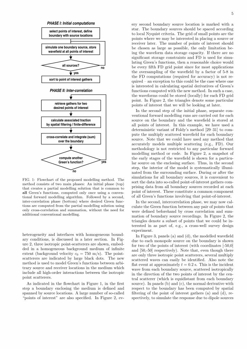
of the boundary sources in as many points as possi-ble throughout the medium. To calculate Green’s func-tion between two points the recordings in the first pointdue to the dipole sources on the boundary are cross-correlated with the recordings in the second point dueto the monopole sources, and vice-versa. The resultingcross-correlations are subtracted and numerically inte-grated over the boundary of source locations. Unprece-dented flexibility follows from the fact that Green’s func-tions can be calculated between all pairs of points thatwere defined up front and stored in the initial bound-ary source modelling phase. Thus, we calculate a partialmodelling solution that is common to all Green’s func-tions, then a bespoke component for each Green function.A flowchart of the new modelling method is given in Fig-ure 1 and is discussed in detail below, in connection withan acoustic isotropic point scattering example.

A. Special case: time-reversal and modelling ofacoustic waves

The time-reversal modelling formula for acoustic wavescan be derived similarly, as discussed in detail by van Ma-nen et al. [1]. Here, we simply state their result, valid forpartially open acoustic media (i.e., with outgoing, radi-ation or absorbing boundary conditions on at least partof the surrounding surface):

G∗pr(x, x′′)−Gpr(x, x′′) =∫

S

1ρ(x′)

[Gpr(x, x′)∇′G∗pr(x

′′, x′)

−∇′Gpr(x,x′)G∗pr(x′′, x′)

] · n dS′, (11)

where Gpr(x, x′′) denotes the Green function for thepressure at location x due to a point source of volumeinjection at location x′′ and ∇′Gpr(x,x′′) · n denotesthe normal derivative of Green’s function with respectto primed coordinates. Thus, the pressure Green func-tion Gpr(x, x′′) between two points x and x′′ can becalculated once the Green functions between the enclos-ing boundary and these points are known. Note thatthe terms Gpr(x,x′′) correspond to simple monopolesources on the surrounding surface whereas the terms∇′Gpr(x, x′′) ·n correspond to dipole sources. This for-mula will be used in the next section to compute theGreen function between points in a 2D acoustic modelwith three isotropic point scatterers embedded in a ho-mogeneous background medium.

IV. EXAMPLE I: 2D ACOUSTIC ISOTROPICPOINT SCATTERING

The methodology described above will now be ex-plained in more detail using a simple 2D acoustic ex-ample. A more realistic elastic model, including strong

5

PHASE I: Initial computations

select points of interest, define

boundary with source locations

simulate one boundary source, store

wavefield at all points of interest

sort to point of interest gathers

all sources?

yes

no

PHASE II: Inter-correlation

cross-correlate and integrate (sum)

over the boundary

retrieve gathers for two

desired points of interest

calculate associated traction

by spatial filtering / finite-difference

compute another

Green’s function? yes

no

FIG. 1: Flowchart of the proposed modelling method. Themethod consists of two main phases: An initial phase (top)that creates a partial modelling solution that is common toall Green’s functions, computed only once using a conven-tional forward modelling algorithm. Followed by a second,inter-correlation phase (bottom) where desired Green func-tions are computed from the partial modelling solution usingonly cross-correlation and summation, without the need foradditional conventional modelling.

heterogeneity and interfaces with homogeneous bound-ary conditions, is discussed in a later section. In Fig-ure 2, three isotropic point-scatterers are shown, embed-ded in a homogeneous background medium of infiniteextent (background velocity c0 = 750 m/s). The point-scatterers are indicated by large black dots. The newmethod is used to model Green’s functions between arbi-trary source and receiver locations in the medium whichinclude all high-order interactions between the isotropicpoint scatterers.

As indicated in the flowchart in Figure 1, in the firststep a boundary enclosing the medium is defined andspanned by source locations. A large number of so-called“points of interest” are also specified. In Figure 2, ev-

ery second boundary source location is marked with astar. The boundary sources should be spaced accordingto local Nyquist criteria. The grid of small points are thepoints where we may be interested in placing a source orreceiver later. The number of points of interest shouldbe chosen as large as possible, the only limitation be-ing the waveform data storage capacity. If there are nosignificant storage constraints and FD is used for simu-lating Green’s functions, then a reasonable choice wouldbe every fifth FD grid point since for most applicationsthe oversampling of the wavefield by a factor of 5-8 inthe FD computations (required for accuracy) is not re-quired – an exception to this could be the case where oneis interested in calculating spatial derivatives of Green’sfunctions computed with the new method. In such a case,the waveforms could be stored (locally) for each FD gridpoint. In Figure 2, the triangles denote some particularpoints of interest that we will be looking at later.

In the second step of the initial phase, separate con-ventional forward modelling runs are carried out for eachsource on the boundary and the wavefield is stored atall points of interest. In this example, we have used adeterministic variant of Foldy’s method [29–31] to com-pute the multiply scattered wavefield for each boundarysource. Note that we could have used any method thataccurately models multiple scattering (e.g., FD). Ourmethodology is not restricted to any particular forwardmodelling method or code. In Figure 2, a snapshot ofthe early stages of the wavefield is shown for a particu-lar source on the enclosing surface. Thus, in the secondstep, the interior of the model is systematically illumi-nated from the surrounding surface. During or after thesimulations for all boundary sources, it is convenient tosort the data into so-called point-of-interest gathers com-prising data from all boundary sources recorded at eachpoint of interest. These constitute a common componentof all Green’s functions involving that point-of-interest.

In the second, intercorrelation phase, we may now cal-culate the Green function between any pair of points thatwere defined beforehand by cross correlation and sum-mation of boundary source recordings. In Figure 2, thetriangles denote a subset of points that we could be in-terested in as part of, e.g., a cross-well survey designexperiment.

In Figure 3, panels (a) and (d), the modelled wavefielddue to each monopole source on the boundary is shownfor two of the points of interest (with coordinates [-50,0]and [50,-50] respectively). Note that, even though thereare only three isotropic point scatterers, several multiplyscattered waves can easily be identified. Also note theflat event at approximately t = 0.2 s. This is the incidentwave from each boundary source, scattered isotropicallyin the direction of the two points of interest by the cen-tral scatterer (which is equidistant from each boundarysource). In panels (b) and (c), the normal derivative withrespect to the boundary has been computed by spatialfiltering of the point of interest gathers (a) and (d), re-spectively, to simulate the response due to dipole sources

6

−100 −80 −60 −40 −20 0 20 40 60 80 100−100

−80

−60

−40

−20

0

20

40

60

80

100

Horizontal coordinate [m]

Ver

tica

l co

ord

inat

e [m

]

FIG. 2: 2D acoustic model and snapshot of a boundarysource wavefield: Three isotropic point scatterers (large blackdots) embedded in a homogeneous background medium c0 =750 m/s of infinite extent. Stars (*) mark every second sourcelocation on a surface enclosing the medium. Small dots (.)mark possible source/receiver locations (so-called points ofinterest) for Green function inter-correlation. Triangles markone of many (cross-well) source/receiver configurations thatcan be evaluated using the new method. In the initial phase,the wavefield is computed for all boundary sources separatelyand stored in all points of interest. A source wavefield isshown for one of the boundary source locations.

on the boundary. This is possible since we have out-going (i.e., absorbing or radiation) boundary conditionson the surrounding surface and hence the pressure andits gradient are directly related (see Appendix B for de-tails). Calculation of the normal derivative with respectto the boundary source location is completely equivalentto measuring the response due to a dipole source so, al-ternatively, we could have modelled the required gradientusing a second dipole source type. Typically, however,direct modelling would be computationally much moreexpensive.

Panels (e) and (f) show the trace-by-trace cross corre-lation of panels (a) and (c) and (b) and (d) respectively.Thus, they form the two terms in the integrand of equa-tion (11). Note that it is difficult to make a straight-forward interpretation of the crosscorrelation panels: al-though equation (11) predicts that the waveform result-ing from summation of these crosscorrelations for allboundary sources will be anti-symmetric in time, pan-els (e) and (f) clearly are not. This is because, at thisstage, we still have not carried through the delicate (butstable!) constructive and destructive interference of theback-propagating wavefield. A more thorough analysis of

the features of such cross correlation gathers is presentedfor the second example. In the final step, crosscorrela-tion gathers (e) and (f) are weighted by ρ−1, subtractedand numerically integrated (summed) over all source lo-cations. The resulting intercorrelation Green functionand a directly computed reference solution are shown inFigure 3(g). The insets show particular events in thewaveform in detail. Note that the reference solution hasbeen slightly shifted vertically to show the match betweenthe overlapping waveforms.

To further illustrate the new modelling method, theintercorrelation phase is now applied repeatedly to cal-culate Green’s functions for the simple cross-well trans-mission and reflection seismic experiment shown in Fig-ure 2 (source and receiver locations are indicated by tri-angles). Note that this does not require any additionalconventional forward modelling but instead uses the samedata modelled in the initial phase. Also note that wecould consider a completely different well location, forany combination of point-of-interests (indicated by smalldots in Figure 2) as long as they were defined beforehandand the wavefield was stored in those points during theinitial modelling phase.

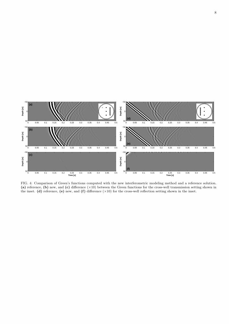
In Figure 4, panels (a) and (b), Green’s functions com-puted using a conventional forward modeling methodand the new method are shown, respectively. The cor-responding source-receiver (transmission) geometry isshown in the inset. Note that the amplitudes have beenscaled up by a factor 5 to show the weak, multiplyscattered events. In panel (c), the difference betweenthe Green functions computed with the two methods isshown and the amplitude differences have been scaledup by an additional factor 10 to emphasize the excel-lent match. Similarly, in panels (d),(e) and (f), Green’sfunctions computed using the new method are comparedto a reference solution for the reflection setting shownin the inset. Again, amplitude (differences) have beenscaled up. In this case by a factor 25 and an additionalfactor 10, respectively. Note the mismatch in the Greenfunction for the direct wave close to the original sourcelocation. This error results from the missing acousticsink and the bandlimited nature of the synthetics, andagrees with the theory presented in section III.

V. EXAMPLE II: 2D ELASTIC PLUTO MODEL

The new methodology is not limited to the particulartype of (idealized) multiple scattering experiment consid-ered above (i.e., the case of isotropic point scatterers em-bedded in a homogeneous background model). As longas the modelling honors the properties of time-reversalinvariance and reciprocity, the new methodology can beapplied. In this section we give a second example of ourmethod for a model that is more relevant to the explo-ration seismic setting. In Figure 5, the compressionalwave velocity in a 4.6 x 4.6 km region of the elastic Plutomodel [32] is shown. This model is often used to bench-

7

Boundary source number

Tim

e [s

](a)

20 40 60 80 100 120 140 160

0

0.1

0.2

0.3

0.4

0.5

Boundary source number

Tim

e [s

]

(c)

20 40 60 80 100 120 140 160

0

0.1

0.2

0.3

0.4

0.5

Boundary source number

Tim

e [s

]

(b)

20 40 60 80 100 120 140 160

0

0.1

0.2

0.3

0.4

0.5

Boundary source number

Tim

e [s

]

(d)

20 40 60 80 100 120 140 160

0

0.1

0.2

0.3

0.4

0.5

Boundary source number

Tim

e [s

]

(e)

20 40 60 80 100 120 140 160

−0.5

−0.4

−0.3

−0.2

−0.1

0

0.1

0.2

0.3

0.4

0.5

Boundary source number

Tim

e [s

]

(f)

20 40 60 80 100 120 140 160

−0.5

−0.4

−0.3

−0.2

−0.1

0

0.1

0.2

0.3

0.4

0.5

−0.5 −0.4 −0.3 −0.2 −0.1 0 0.1 0.2 0.3 0.4 0.5

−1

−0.5

0

0.5

1

Time [s]

(g)

FIG. 3: Modelled waveforms for all boundary sources in two points of interest and their cross-correlation: (a) Monopoleresponse in point [-50,0] and (b) corresponding dipole response computed by spatial filtering [see text for details]. (c) Dipoleresponse in point [50,-50] computed by spatial filtering and (d) corresponding monopole response. (e) Cross correlation of (a)and (c). (f) Cross correlation of (b) and (d). The difference between gathers (e) and (f),weighted by ρ−1, forms the integrandof equation (11). (g) Intercorrelation Green function (green) and a directly computed reference solution (blue). Insets showdetails of the signals in time-intervals bounded by dashed boxes. Note the anti-symmetry of the intercorrelation Green functionacross t = 0 s, as predicted by equation (11). The waveforms have been slightly offset vertically from each other to betterillustrate the match.

8

(b)

Dep

th [

m]

0 0.05 0.1 0.15 0.2 0.25 0.3 0.35 0.4 0.45 0.5

−50

0

50

Dep

th [

m]

Time [s]

(c)

0 0.05 0.1 0.15 0.2 0.25 0.3 0.35 0.4 0.45 0.5

−50

0

50

(a)

Dep

th [

m]

0 0.05 0.1 0.15 0.2 0.25 0.3 0.35 0.4 0.45 0.5

−50

0

50

(e)

Dep

th [

m]

0 0.05 0.1 0.15 0.2 0.25 0.3 0.35 0.4 0.45 0.5

−50

0

50

Dep

th [

m]

Time [s]

(f)0 0.05 0.1 0.15 0.2 0.25 0.3 0.35 0.4 0.45 0.5

−50

0

50

(d)D

epth

[m

]0 0.05 0.1 0.15 0.2 0.25 0.3 0.35 0.4 0.45 0.5

−50

0

50

FIG. 4: Comparison of Green’s functions computed with the new interferometric modeling method and a reference solution.(a) reference, (b) new, and (c) difference (×10) between the Green functions for the cross-well transmission setting shown inthe inset. (d) reference, (e) new, and (f) difference (×10) for the cross-well reflection setting shown in the inset.

9

X−coordinate (m)

Dep

th (

m)

1.9 1.95 2 2.05 2.1 2.15 2.2 2.25 2.3

x 104

0

500

1000

1500

2000

2500

3000

3500

4000

Com

pres

sion

al v

eloc

ity (

m/s

)

1600

1800

2000

2200

2400

2600

2800

FIG. 5: P-wave velocity of a 2D elastic marine seismic model[32]. The color scale is clipped to display weak velocity con-trasts (P-wave velocity of salt is 4500 m/s).

mark marine seismic imaging algorithms. A high velocity(4500 m/s) salt body on the right represents a commonimaging challenge. In black, two points of interest (offset1 km) are shown. The dotted line denotes the boundarywith NS = 1200 source locations distributed with a den-sity consistent with the local spatial Nyquist frequency,which means that the wavefield should not be aliasedin the point of interest gathers. Outgoing (i.e., radia-tion or absorbing) boundary conditions [33] are appliedright outside the surface enclosing the points of interestto truncate the computational domain.

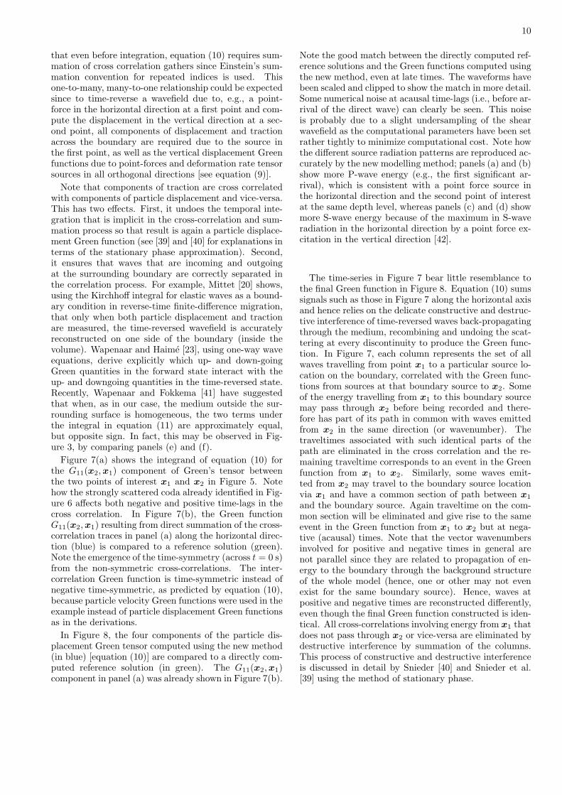
Forward simulations were carried out for each of the1200 source locations on the boundary using an elasticFD code [34] and the waveforms (components of particledisplacement) stored at 90,000 points distributed regu-larly throughout the model. Since we are dealing with the2D elastodynamic wave equation, at least two forwardsimulations have to be carried out for each source loca-tion: one for each unidirectional point force in mutuallyorthogonal directions. Figure 6 shows the first 4 secondsof the G11(x1,x

′) component of Green’s tensor modelledfor the left point of interest (i.e., the horizontal compo-nent of particle displacement in the point of interest x1

due to all point-force sources in the horizontal directionon the boundary at locations x′). For reference, the firstsource on the boundary is located just below the freesurface on the right in Figure 5, at 2.56 m depth in thewater layer. The last source on the boundary is locatedjust below the free surface on the left. Note that becauseof the cross-symmetry of the terms in the integrand inequation (10), no sources are required along the Earth’sfree surface, or any interface with homogeneous bound-ary conditions (e.g., with either vanishing traction [Neu-mann] or vanishing particle displacement [Dirichlet]). In-tuitively, this can be understood from a method of imag-ing argument: since such interfaces act as perfect mirrors,

reflecting all energy back into the volume, an equivalentmedium can be constructed which consists of the origi-nal medium combined with its mirror in the homogeneousboundary and the homogeneous boundary absent. Sincethe original boundary with source locations is mirroredas well, the new boundary does completely surround thishypothetical medium and therefore, the sources consti-tute a perfect time-reversal mirror in the sense describedby Derode et al. [2]. Note that when the free surface hastopography, although the method of imaging argumentbreaks down, this property still holds.

An interesting feature of the data, to which we willreturn later, occurs approximately between sources 200-475, and between sources 1800-2200. These sources arelocated in the near-surface of the sedimentary column,just beneath the water layer. The Pluto model includesmany randomly positioned, near-surface scatterers, rep-resenting complex near-surface heterogeneity that is of-ten observed in nature. Within these two source ranges itis clear that all coherent arrivals are followed by compli-cated codas that are superposed, resulting in a multiply-scattered signal that builds with time.

Note that according to equation (10) derivatives of theGreen function with respect to the source location onthe boundary also have to be computed. These termscorrespond to the response due to special (deformationrate tensor) sources on the boundary and seem to re-quire additional modelling with such special sources be-fore Green’s functions can be computed using the newmethod. However, using reciprocity, these terms can alsobe interpreted as the traction measured on the enclos-ing boundary due to unidirectional point forces at a par-ticular point of interest. When the surface surroundingthe medium has outgoing boundary conditions, the wavefield and the corresponding traction are directly related[25]. In Appendix B, it is explained in detail how theseproperties can be exploited to avoid the need for addi-tional direct modelling. Briefly, when the wavefield isexcited on a straight boundary, embedded in a laterallyhomogeneous medium (where lateral means along the ar-ray), the reciprocal components of particle displacementin the point of interest gather are Fourier transformedinto the frequency-wavenumber domain and matrix mul-tiplication with an analytical expression gives the cor-responding components of traction before transformingback to the space-time domain. When the boundary iscurved and/or the medium is not homogeneous along thesource array, spatially compact filter approximations canbe designed to filter the data in the space-frequency do-main using space-variant convolution. This approach isakin to, e.g., decomposition of multi-component seismicdata in the common shot domain using spatially compactfilters, where it gives promising results [35–38].

When all stored components of the Green tensor havebeen retrieved for two points of interest and the corre-sponding equivalent traction data are computed throughspatial filtering, the point of interest gathers are cross-correlated and summed according to equation (10). Note

10

that even before integration, equation (10) requires sum-mation of cross correlation gathers since Einstein’s sum-mation convention for repeated indices is used. Thisone-to-many, many-to-one relationship could be expectedsince to time-reverse a wavefield due to, e.g., a point-force in the horizontal direction at a first point and com-pute the displacement in the vertical direction at a sec-ond point, all components of displacement and tractionacross the boundary are required due to the source inthe first point, as well as the vertical displacement Greenfunctions due to point-forces and deformation rate tensorsources in all orthogonal directions [see equation (9)].

Note that components of traction are cross correlatedwith components of particle displacement and vice-versa.This has two effects. First, it undoes the temporal inte-gration that is implicit in the cross-correlation and sum-mation process so that result is again a particle displace-ment Green function (see [39] and [40] for explanations interms of the stationary phase approximation). Second,it ensures that waves that are incoming and outgoingat the surrounding boundary are correctly separated inthe correlation process. For example, Mittet [20] shows,using the Kirchhoff integral for elastic waves as a bound-ary condition in reverse-time finite-difference migration,that only when both particle displacement and tractionare measured, the time-reversed wavefield is accuratelyreconstructed on one side of the boundary (inside thevolume). Wapenaar and Haime [23], using one-way waveequations, derive explicitly which up- and down-goingGreen quantities in the forward state interact with theup- and downgoing quantities in the time-reversed state.Recently, Wapenaar and Fokkema [41] have suggestedthat when, as in our case, the medium outside the sur-rounding surface is homogeneous, the two terms underthe integral in equation (11) are approximately equal,but opposite sign. In fact, this may be observed in Fig-ure 3, by comparing panels (e) and (f).

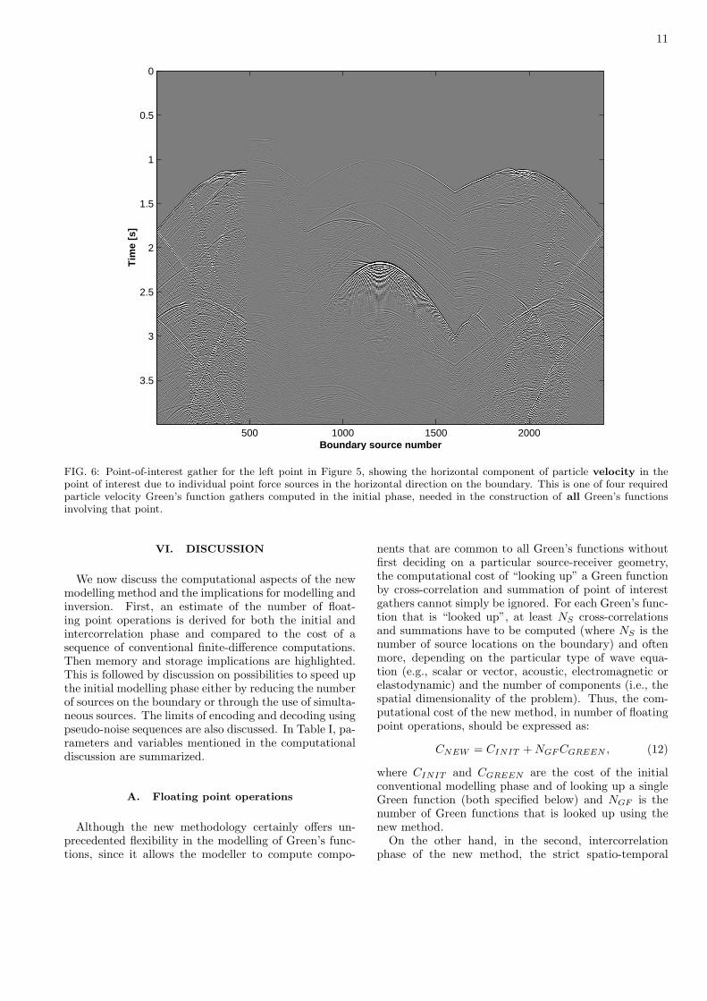
Figure 7(a) shows the integrand of equation (10) forthe G11(x2, x1) component of Green’s tensor betweenthe two points of interest x1 and x2 in Figure 5. Notehow the strongly scattered coda already identified in Fig-ure 6 affects both negative and positive time-lags in thecross correlation. In Figure 7(b), the Green functionG11(x2, x1) resulting from direct summation of the cross-correlation traces in panel (a) along the horizontal direc-tion (blue) is compared to a reference solution (green).Note the emergence of the time-symmetry (across t = 0 s)from the non-symmetric cross-correlations. The inter-correlation Green function is time-symmetric instead ofnegative time-symmetric, as predicted by equation (10),because particle velocity Green functions were used in theexample instead of particle displacement Green functionsas in the derivations.

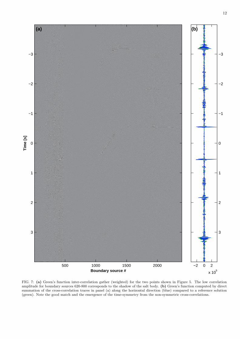
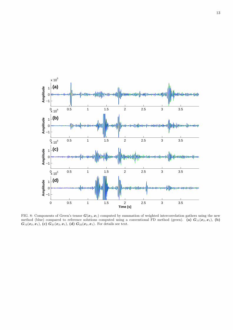
In Figure 8, the four components of the particle dis-placement Green tensor computed using the new method(in blue) [equation (10)] are compared to a directly com-puted reference solution (in green). The G11(x2,x1)component in panel (a) was already shown in Figure 7(b).

Note the good match between the directly computed ref-erence solutions and the Green functions computed usingthe new method, even at late times. The waveforms havebeen scaled and clipped to show the match in more detail.Some numerical noise at acausal time-lags (i.e., before ar-rival of the direct wave) can clearly be seen. This noiseis probably due to a slight undersampling of the shearwavefield as the computational parameters have been setrather tightly to minimize computational cost. Note howthe different source radiation patterns are reproduced ac-curately by the new modelling method; panels (a) and (b)show more P-wave energy (e.g., the first significant ar-rival), which is consistent with a point force source inthe horizontal direction and the second point of interestat the same depth level, whereas panels (c) and (d) showmore S-wave energy because of the maximum in S-waveradiation in the horizontal direction by a point force ex-citation in the vertical direction [42].

The time-series in Figure 7 bear little resemblance tothe final Green function in Figure 8. Equation (10) sumssignals such as those in Figure 7 along the horizontal axisand hence relies on the delicate constructive and destruc-tive interference of time-reversed waves back-propagatingthrough the medium, recombining and undoing the scat-tering at every discontinuity to produce the Green func-tion. In Figure 7, each column represents the set of allwaves travelling from point x1 to a particular source lo-cation on the boundary, correlated with the Green func-tions from sources at that boundary source to x2. Someof the energy travelling from x1 to this boundary sourcemay pass through x2 before being recorded and there-fore has part of its path in common with waves emittedfrom x2 in the same direction (or wavenumber). Thetraveltimes associated with such identical parts of thepath are eliminated in the cross correlation and the re-maining traveltime corresponds to an event in the Greenfunction from x1 to x2. Similarly, some waves emit-ted from x2 may travel to the boundary source locationvia x1 and have a common section of path between x1

and the boundary source. Again traveltime on the com-mon section will be eliminated and give rise to the sameevent in the Green function from x1 to x2 but at nega-tive (acausal) times. Note that the vector wavenumbersinvolved for positive and negative times in general arenot parallel since they are related to propagation of en-ergy to the boundary through the background structureof the whole model (hence, one or other may not evenexist for the same boundary source). Hence, waves atpositive and negative times are reconstructed differently,even though the final Green function constructed is iden-tical. All cross-correlations involving energy from x1 thatdoes not pass through x2 or vice-versa are eliminated bydestructive interference by summation of the columns.This process of constructive and destructive interferenceis discussed in detail by Snieder [40] and Snieder et al.[39] using the method of stationary phase.

11

Boundary source number

Tim

e [s

]

500 1000 1500 2000

0

0.5

1

1.5

2

2.5

3

3.5

FIG. 6: Point-of-interest gather for the left point in Figure 5, showing the horizontal component of particle velocity in thepoint of interest due to individual point force sources in the horizontal direction on the boundary. This is one of four requiredparticle velocity Green’s function gathers computed in the initial phase, needed in the construction of all Green’s functionsinvolving that point.

VI. DISCUSSION

We now discuss the computational aspects of the newmodelling method and the implications for modelling andinversion. First, an estimate of the number of float-ing point operations is derived for both the initial andintercorrelation phase and compared to the cost of asequence of conventional finite-difference computations.Then memory and storage implications are highlighted.This is followed by discussion on possibilities to speed upthe initial modelling phase either by reducing the numberof sources on the boundary or through the use of simulta-neous sources. The limits of encoding and decoding usingpseudo-noise sequences are also discussed. In Table I, pa-rameters and variables mentioned in the computationaldiscussion are summarized.

A. Floating point operations

Although the new methodology certainly offers un-precedented flexibility in the modelling of Green’s func-tions, since it allows the modeller to compute compo-

nents that are common to all Green’s functions withoutfirst deciding on a particular source-receiver geometry,the computational cost of “looking up” a Green functionby cross-correlation and summation of point of interestgathers cannot simply be ignored. For each Green’s func-tion that is “looked up”, at least NS cross-correlationsand summations have to be computed (where NS is thenumber of source locations on the boundary) and oftenmore, depending on the particular type of wave equa-tion (e.g., scalar or vector, acoustic, electromagnetic orelastodynamic) and the number of components (i.e., thespatial dimensionality of the problem). Thus, the com-putational cost of the new method, in number of floatingpoint operations, should be expressed as:

CNEW = CINIT + NGF CGREEN , (12)

where CINIT and CGREEN are the cost of the initialconventional modelling phase and of looking up a singleGreen function (both specified below) and NGF is thenumber of Green functions that is looked up using thenew method.

On the other hand, in the second, intercorrelationphase of the new method, the strict spatio-temporal

12

Boundary source #

Tim

e [s

](a)

500 1000 1500 2000

−3

−2

−1

0

1

2

3

−2 0 2

x 105

−3

−2

−1

0

1

2

3

(b)

FIG. 7: (a) Green’s function inter-correlation gather (weighted) for the two points shown in Figure 5. The low correlationamplitude for boundary sources 620-800 corresponds to the shadow of the salt body. (b) Green’s function computed by directsummation of the cross-correlation traces in panel (a) along the horizontal direction (blue) compared to a reference solution(green). Note the good match and the emergence of the time-symmetry from the non-symmetric cross-correlations.

13

0 0.5 1 1.5 2 2.5 3 3.5

−1

0

1

x 105

Am

plit

ud

e (a)

0 0.5 1 1.5 2 2.5 3 3.5

−1

0

1

x 105

Am

plit

ud

e (b)

0 0.5 1 1.5 2 2.5 3 3.5

−1

0

1

x 105

Am

plit

ud

e (c)

0 0.5 1 1.5 2 2.5 3 3.5

−1

0

1

x 105

Am

plit

ud

e

Time [s]

(d)

FIG. 8: Components of Green’s tensor G(x2, x1) computed by summation of weighted intercorrelation gathers using the newmethod (blue) compared to reference solutions computed using a conventional FD method (green). (a) G11(x2, x1), (b)G12(x2, x1), (c) G21(x2, x1), (d) G22(x2, x1). For details see text.

14

parameter description unitsfmax maximum frequency 1/scmin minimum velocity m/scmax maximum velocity m/s∆X finite-difference grid spacing m∆T finite-difference timestep sa number of operations to evaluate the discrete temporal and spa-

tial derivatives (dimension and wave-equation dependent)flops

b time sub-sampling factor dimensionlessc number of cross-correlations required for a single component of

Green’s tensordimensionless

n dimension of the modeling dimensionlessm number of source components dimensionlessγ Courant stability number (code dependent) dimensionlessCFD cost of a single finite-difference run flopsCFFT cost of a combined FFT of two, padded real-valued traces flopsCGREEN cost of a single Green function intercorrelation flopsCINIT cost of the initial phase in the new method flopsCCONV cost of a conventional sequence of FD simulations flopsCNEW cost using the new methodology to compute Green functions flopsNX number of gridpoints along a typical dimension dimensionlessNT number of timesteps in the initial FD computations dimensionlessNT ′ number of timesteps in the inter-correlation phase dimensionlessNS number of source locations on the boundary dimensionlessNGF number of Green’s function intercorrelations dimensionlessNM minimum number of conventional sources or receivers dimensionlessN number of points of interest dimensionless

TABLE I: Description of all parameters and variables mentioned in the computational discussion

sampling requirements of a typical full waveform mod-elling method (as governed by numerical accuracy andthe Courant criterion) can be relaxed to Nyquist crite-ria. For example, in Appendix C it is shown that for atypical acoustic 2D finite-difference code with 2nd orderaccuracy in time and 4th order accuracy in space [de-noted FD(2,4)], the ratio b between the time step ∆T ′ inthe intercorrelation phase and the time step ∆T in theconventional modelling phase is:

b ≡ ∆T ′

∆T=

NT

NT ′≈ 4

γ

(cmax

cmin

), (13)

where cmax and cmin are the maximum and minimumvelocity in the medium, respectively and γ is a constantrelating to the specific FD code. For the FD(2,4) codeγ = 0.45. NT and NT ′ are the number of time samples inthe initial and intercorrelation phase respectively. Tak-ing the maximum frequency fmax in the final seismogramfmax = 75 Hz, cmin = 1500 m/s and cmax = 4500 m/s(salt) gives the ratio b = 26.67. Thus, the cost of look-ing up a Green function in the intercorrelation phase issubstantially reduced by abandoning the oversampling.

In addition, to further reduce the cost of lookingup Green’s functions, waveforms modelled in the initialphase are stored in the frequency domain in anticipa-tion of the cross correlations in the intercorrelation phase(multiplication with the complex conjugate). This avoidshaving to recompute the Fourier transform of point ofinterest gathers when computing several Green functionsinvolving the same point of interest.

In Appendix C it is shown that, based on the re-laxed sampling requirements and use of the fast Fouriertransform (FFT) to compute cross-correlations as out-lined above, the total number of floating point operation(flops) required for the look-up of one component of asingle Green tensor CGREEN is:

CGREEN ∼ (8c + 2)NSNT ′ , (14)

where c is the number of cross-correlations that need tobe computed for a single boundary source location whenone component of Green’s tensor is looked-up. Hence, cdepends on the the type of wave equation (i.e., scalar orvector) and the spatial dimensionality of the problem, n.In Appendix C, c is computed for the cases of two- andthree-dimensional, acoustic and elastic modelling. Theresults are summarized in Table II. In equation (14) thecost of Fourier transforming the intercorrelation Greenfunction back to the time-domain has been neglected asexplained in Appendix C.

Note that using the new method, the simulation timeT has to be longer than in a conventional FD simulation.This can be understood by considering the reciprocal ex-periment in which one of two points of interest acts as asource: any energy that we want to time-reverse has to berecorded on the surrounding boundary. This means, e.g.,that a particular (multiply scattered) wave in the Greenfunction between the two points has to have had enoughtime to reach the boundary from that second point inorder to be time-reversed. In general the initial FD sim-ulations need to run long enough such that most energy

15

has left the grid. In the following we assume that thisdoubles the simulation time for the new method.

The computational cost of both the initial modellingphase and a sequence of conventional finite-differencesimulations is proportional to CFD, the number of flopsrequired for a single conventional FD simulation. In turn,CFD is proportional to the number of gridpoints in eachof n dimensions, NX , timesteps NT and the number offlops, a, required for the evaluation of the discrete tem-poral and spatial derivatives [e.g., a = 22 for a typicalacoustic 2D FD code (see Table II)]. Thus we have:

CFD ∼ aNT NnX . (15)

Based on the above considerations, the number of float-ing point operations for a sequence of NM conventionalFD calculations and for the new method now can be com-pared as [Appendix C, equation (C8)]:

CCONV =12mNMCFD (16)

CNEW = mNSCFD + m2NGF CGREEN , (17)

where m = 1 in case of acoustic modelling and m = n incase of elastic modelling and NM is the minimum of thenumber of source and receiver locations considered in themodelling.

Case 1: NGF = NM The new method is particu-larly attractive in applications where Green’s functionsare desired between a large number of points interior toa medium, but where there are no common source or re-ceiver points. In such a case, a separate conventional FDsimulation is required for each Green tensor and, hence,NGF = NM . In this case, equations (16) and (17) are astraight line through zero and a vertically offset straightline, as a function of NM , respectively and the newmethod becomes more efficient beyond the intersectionpoint of the two lines. No other existing method couldoffer full waveforms at comparable computational cost.The method also offers great flexibility where the exactinterior points are not known in advance since Green’sfunctions can be computed on an “as needed” basis fromGreen’s functions between points on the surrounding sur-face and its interior. We have shown how the latter Greenfunctions constitute a common component of all Greenfunctions in the medium through equation (10).

Case 2: NGF ∼ N2M When the number of sources

and receivers are approximately equal and one is in-terested in computing Green’s functions for all possiblesource/receiver combinations, the number of Green func-tions to be looked up NGF is proportional to the squareof the number of source/receiver points NM : NGF ∼ N2

Mand the new method may actually be less efficient than asequence of conventional FD simulations. In such a case,equations (16) and (17) are a straight line through zeroand a vertically offset parabola, as a function of NM , re-spectively and, at best, there may be a region where thenew method is more computationally efficient.

B. Memory and storage

Assuming that a standard isotropic elastic FD methodis used (e.g., not relying on domain decomposition), theamount of run-time memory required for storage of the(n/2)(n + 3) field quantities (e.g., vi and σij) and 3medium parameters (e.g., ρ, λ and µ) in run-time mem-ory requires at least 4[(n/2)(n + 3) + 3]Nn

X bytes (fora heterogeneous medium and calculations carried outin single precision). We note that for a medium sizeof NX = 1000, a 3D elastic problem will require onthe order of 45 Gbytes of primary memory. This num-ber grows considerably for even more complex media(e.g., anisotropic), and the computations therefore typi-cally rely on large shared memory machines or heavilyparallelized algorithms running on clusters with high-performance connections. Using our methodology wecompute a table of all point of interest gathers usinghigh-end computational resources. The computations inthe intercorrelation phase, on the other hand, would beperformed on much smaller machines as they require asubstantially smaller amount of primary memory and be-cause they require only a subset of the inter-correlationtable to be exported. We have shown how the point of in-terest gathers with Green functions constitute a commoncomponent of all Green functions in the medium throughequation (10).

C. Simultaneous sources: limits ofencoding and decoding

We also investigated exciting the boundary sourcessimultaneously by encoding the source signals us-ing pseudo-noise sequences [43] and with simultaneoussources distributed randomly in the medium [2] as twoalternative ways to reduce the number of sources, andhence, the computational cost of the initial forward mod-elling phase. Such approaches have been investigated inattempts to speed-up conventional finite-difference sim-ulations, although in surprisingly few published studies.Recent experimental evidence in passive imaging how-ever, using techniques based on interferometry and time-reversal, seems to suggest that such an approach wouldbe highly feasible for the new modelling method. Forinstance, Wapenaar and Fokkema [10] and Derode et al.[2] show that, when the sources surrounding and insidethe medium consist of uncorrelated noise sequences, theirautocorrelation tends to a delta function and terms in-volving crosscorrelations between the different noise se-quences can be ignored. However, it is well known inthe field of communications analysis that Welch’s bound(Welch [44]) poses a fundamental limit to the qualityof separation of such pseudo-noise sequences of a givenlength, when emitted simultaneously. In Appendix Dit is shown that, when making no assumptions aboutthe Green function, the signal-to-interference (from theunwanted cross-correlations between the encoding se-

16

Acoustic Elasticparameter 2D 3D 2D 3D

a 22 32 50 102m 1 1 n(= 2) n(= 3)

c(= 2m) 2 2 4 6

TABLE II: Values for the different parameters in 2D and 3D acoustic and elastic modelling

quences) ratio in the final modelled seismogram is pro-portional to ∼ √

N , where N is the length of the se-quences. Thus, the signal-to-interference ratio only im-proves as the square-root of the sequence length. Notethat the number of sequences required, the so-called fam-ily size M (equal to the number of boundary sources:M = NS), does not influence the signal-to-interferenceratio. A similar expression was recently derived bySnieder [40] using a statistical approach to explain theemergence of the ballistic (direct wave) Green functionthrough an ensemble of scatterers with uncorrelated po-sitions.

Although in principle, and in real-life experiments, itis possible to reduce such interference by time/event av-eraging, where data is “modelled” for free and all wehave to do is listen longer [40], in synthetic modelling ofGreen’s functions it is exactly the modelling itself that isexpensive and therefore the use of pseudo-noise sequencesfor the purpose of interferometric, simultaneous sourceFD modelling is probably limited. In all explored cases,the limits of separation caused relatively high noise lev-els compared to the equivalent FD effort using the directmethod described above.

D. High-order approximations

Whereas traditional approximate modelling methodstypically impose restrictions with respect to the degreeof heterogeneity in the medium of propagation or ne-glect high-order scattering, the new time-reversal mod-elling methodology allows us instead to compromise onnoise level while maintaining high-order scattering andfull heterogeneity in the medium. Recent experimentaland theoretical work indicates that time-reversed imag-ing is robust with respect to perturbations in the bound-ary conditions [2, 30]. For cases where the wave propaga-tion is heavily dominated by multiple scattering even asingle source may be sufficient to excite all wavenumbersin the model, and hence to refocus essential parts of atime-reversed signal [45]. Even when not all wavenum-bers are excited by a single source, such as in the ex-amples above, it may be possible to substantially reducethe number of sources and still recover essential parts ofthe signal. van Manen et al. [1] showed that even for asfew as one sixteenth of the original number of sourcesthey were able to reproduce amplitude and phase of anarrival of interest fairly accurately, but with an increasednoise level. Clearly, the required number of sources willdepend on the application. For many applications, the

possibility to trade-off signal-to-noise ratio to CPU timewithout compromising on medium complexity or high-order scattering will be another attractive property ofthe new method.

E. Synergies with inverse theory

We anticipate that the new methodology will also havea significant impact on inversion since in some related ar-eas relevant theory has already been developed. For ex-ample, Oristaglio [28] has shown that the Porter-Bojarskiintegral [equation (9)] forms the basis for an inverse scat-tering formula that uses all the data. He proved that athree step imaging procedure, consisting of backpropaga-tion (or focusing) of receiver and source arrays and tem-poral filtering, gives the scattering potential within theBorn approximation. His formula also relies on completeillumination of a (three-dimensional) scattering objectfrom a surface surrounding the object as our modelingmethod does. Rose [46] argues that focusing, combinedwith time-reversal is the physical basis of exact inversescattering and derives the Newton-Marchenko equationfrom these two principles.

In cases where the medium is relatively well known,but where the objective is to track some kind of non-stationary source within the volume, again the flexibilityof the new method is a significant advantage, especiallyif the receivers are also non-stationary.

The new method also provides a flexible way to com-pute spatial derivatives of the intercorrelation Greenfunctions with respect to both source and receiver coordi-nates for any region in the model, provided the points ofinterest are spaced closely enough in the initial modelingphase (as mentioned above, the spacing is only subjectto storage limitations and does not influence the com-putational cost). This means that it is straightforwardto consider other types of sources, such as pure P- andS-wave sources and detectors that are only sensitive toP- or S-waves (see e.g., [23] and [35]). Alternatively, thenew modelling method could have been formulated di-rectly in terms of crosscorrelations of Green functions forpure P- and S-wave sources on the boundary and pureP- and S-wave receivers in the points of interest [5].

Another interesting aspect of the method is that it pro-vides exactly those Green functions required for directevaluation of higher-order terms in the Neumann seriessolution to multiple scattering. To illustrate this, con-sider again the case of isotropic point scatterers embed-ded in a homogeneous background medium. The complex

17

scattering coefficient of scatterer i is denoted Ai. Sniederand Scales [30] show that the total multiply scatteredwavefield u(x) at location x due to the (unperturbed)incident wavefield u(0)(x) can be written as:

u(x) = u(0)(x) +∑

i

G(x, xi)Aiu(0)(xi)

+∑

i 6=j G(x, xi)AiG(xi, xj)Aju(0)(xj) + · · · , (18)

where G(xi,xj) denotes Green’s function in the back-ground medium between (scatterer) locations xj and xi.This is the Neumann series solution. The first term onthe r.h.s., u(0)(x), corresponds to the incident wavefieldmeasured at the receiver location (propagating in thebackground medium). The second term corresponds tothe Born (single scattering) approximation. The thirdterm is a double summation over all possible paths in-cluding two scatterers, where the same scatterer cannotbe visited on consecutive scattering events. Note thatall Green functions in equation (18) (between scatterersand between scatterers and the observation point) can becomputed efficiently using the new method. For the ex-ample of a homogeneous background medium given here,the required Green functions are simply free-space Greenfunctions and the computation is trivial. However, equa-tion (18) is easily generalized to the case of small per-turbations with respect to more complicated backgroundmedia and although the summations become volume in-tegrations, the form of the Neumann series solution staysthe same. In such cases, computation of the Green func-tions in the background medium may not be trivial andthe new method provides such Green functions efficientlyand flexibly. Note that we do not even have to specifybeforehand which regions of the model we want to per-turb.

Thus, we have shown how recent insights into the rela-tionship between Green’s theorem and time-reversal canbe extended to modelling of wave propagation by invok-ing reciprocity. We expect that this may significantlychange the way we approach modelling and inversion ofthe wave equation in future.

APPENDIX A: THE ELASTODYNAMICRECIPROCITY THEOREM

Here, for completeness, we derive the elastodynamicreciprocity theorem. We closely follow Snieder [26]. Theelastodynamic reciprocity theorem relates two states (A)and (B) that can occur in the same medium indepen-dently:

ρω2u(A)i + ∂j

(cijkl∂ku

(A)l

)= −f

(A)i ,

ρω2u(B)i + ∂j

(cijkl∂ku

(B)l

)= −f

(B)i , (A1)

where u(A) and u(B) are particle displacements forstates (A) and (B), generated by excitations f (A) and

f (B) respectively. The representation theorem can bederived by multiplying the first equation by u

(B)i and the

second by u(A)i and subtracting the results and integrat-

ing over a volume V :∫

V

{u

(B)i ∂j

(cijkl∂ku

(A)l

)

−u(A)i ∂j

(cijkl∂ku

(B)l

)}dV

= −∫

V

{f

(A)i u

(B)i − f

(B)i u

(A)i

}dV. (A2)

The first term in curly brackets on the left hand side canbe identified as one part of the integrated product rulefor differentiation:

∫

V

u(B)i ∂j

(cijkl∂ku

(A)l

)dV =

∫

V

∂j

(u

(B)i cijkl∂ku

(A)l

)dV

−∫

V

(∂ju

(B)i

)cijkl∂ku

(A)l dV. (A3)

and the second term can be interpreted similarly. In-serting these expressions and using Gauss’s theorem toconvert volume integrals to surface integrals, we get:

∫

S

{u

(B)i njcijkl∂ku

(A)l − u

(A)i njcijkl∂ku

(B)l

}dS

−∫

V

{(∂ju

(B)i

)cijkl

(∂ku

(A)l

)

−(∂ju

(A)i

)cijkl

(∂ku

(B)l

)}dV

= −∫

V

{f

(A)i u

(B)i − f

(B)i u

(A)i

}dV. (A4)

Note that the second term on the left hand side disap-pears because of the symmetry properties of the elasticitytensor: cijkl = cklij . Thus we have:

∫

S

{u

(B)i njcijkl∂ku

(A)l − u

(A)i njcijkl∂ku

(B)l

}dS

= −∫

V

{f

(A)i u

(B)i − f

(B)i u

(A)i

}dV. (A5)

Note that the reciprocity theorem can be derived fromthis expression by assuming homogeneous boundary con-ditions and identifying both states (A) and (B) witha mathematical or Green state (i.e., a state involv-ing Green’s functions rather than measured quantities[10, 26]). In the main text, equation (A5) is used toderive the representation theorem.

APPENDIX B: COMPUTATION OF THEGRADIENT BY SPATIAL FILTERING

It is well known that when the wave field on a boundarysatisfies outgoing (i.e., radiation or absorbing) boundary

18

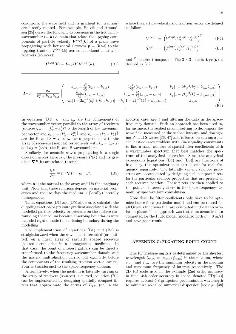
conditions, the wave field and its gradient (or traction)are directly related. For example, Holvik and Amund-sen [25] derive the following expressions in the frequency-wavenumber (ω, k)-domain that relate the upgoing com-ponents of particle velocity V (up)(k) of a plane wavepropagating with horizontal slowness p = (k/ω) to theupgoing traction T (up)(k) across a horizontal array ofreceivers (sources):

T (up)(k) = LTV (k)V (up)(k), (B1)

where the particle velocity and traction vector are definedas follows:

V (up) =(V

(up)1 , V

(up)2 , V

(up)3

)T

(B2)

T (up) =(T

(up)1 , T

(up)2 , T

(up)3

)T

(B3)

and T denotes transposed. The 3 × 3 matrix LTV (k) isderived as [25]:

LTV =ρω

k2r + kz,αkz,β

kz,α − k2y

k2β(kz,α − kz,β) kxky

k2β

(kz,α − kz,β) kx[1− 2k−2β (k2

r + kz,αkz,β)]kxky

k2β

(kz,α − kz,β) kz,α − k2x

k2β(kz,α − kz,β) ky[1− 2k−2

β (k2r + kz,αkz,β)]

−kx[1− 2k−2β (k2

r + kz,αkz,β)] −ky[1− 2k−2β (k2

r + kz,αkz,β)] kz,β .

(B4)

In equation (B4), kx and ky are the components ofthe wavenumber vector parallel to the array of receivers(sources), kr = (k2

x + k2y)

12 is the length of the wavenum-

ber vector and kz,α = (k2α − k2

r)12 and kz,β = (k2

β − k2r)

12

are the P- and S-wave slownesses perpendicular to thearray of receivers (sources) respectively with kα = (ω/α)and kβ = (ω/α) the P- and S-wavenumbers.

Similarly, for acoustic waves propagating in a singledirection across an array, the pressure P (k) and its gra-dient ∇P (k) are related through:

∂P

∂n≡ n ·∇P = ikz,αP, (B5)

where n is the normal to the array and i is the imaginaryunit. Note that these relations depend on material prop-erties and require that the medium is (locally) laterallyhomogeneous.

Thus, equations (B1) and (B5) allow us to calculate theoutgoing traction or pressure gradient associated with themodelled particle velocity or pressure on the surface sur-rounding the medium because absorbing boundaries wereincluded right outside the enclosing boundary during themodelling.

The implementation of equations (B1) and (B5) isstraightforward when the wave field is recorded (or emit-ted) on a linear array of regularly spaced receivers(sources) embedded in a homogeneous medium. Inthat case, the point of interest gathers can be directlytransformed to the frequency-wavenumber domain andthe matrix multiplication carried out explicitly beforethe components of the resulting traction vector inverse-Fourier transformed to the space-frequency domain.

Alternatively, when the medium is laterally varying orthe array of receivers (sources) is curved, equation (B1)can be implemented by designing spatially compact fil-ters that approximate the terms of LTV (or, in the

acoustic case, iωqα) and filtering the data in the space-frequency domain. Such an approach has been used in,for instance, the seabed seismic setting to decompose thewave field measured at the seabed into up- and downgo-ing P- and S-waves [36, 47] and is based on solving a lin-ear least-squares problem with (in-)equality constraintsto find a small number of spatial filter coefficients witha wavenumber spectrum that best matches the spec-trum of the analytical expression. Since the analyticalexpressions [equations (B4) and (B5)] are functions offrequency, this optimization is carried out for each fre-quency separately. The laterally varying seafloor prop-erties are accomodated by designing such compact filtersfor the particular seafloor properties that are present ateach receiver location. These filters are then applied tothe point of interest gathers in the space-frequency do-main by space-variant convolution.

Note that the filter coefficients only have to be opti-mized once for a particular model and can be reused forall Green’s functions that are computed in the intercorre-lation phase. This approach was tested on acoustic datacomputed for the Pluto model (modelled with β = 0 m/s)and gave good results.

APPENDIX C: FLOATING POINT COUNT

The FD gridspacing ∆X is determined by the shortestwavelength λmin = (cmin/fmax) in the medium, wherecmin and fmax are the minimum velocity in the mediumand maximum frequency of interest respectively. The2D FD code used in the example [2nd order accuracyin time, 4th order accuracy in space, denoted FD(2,4)]requires at least 5-8 gridpoints per minimum wavelengthto minimize so-called numerical dispersion [see e.g., [48]

19

and [34]], thus:

∆X ≤ λmin

8=

cmin

8fmax. (C1)

The time step ∆T in the FD simulation is determined bythe Courant stability criterion:

∆T ≤ γ∆X

cmax=

γ

8fmax

(cmin

cmax

), (C2)

where γ is a constant relating to the specific FD code. Forthe FD(2,4) code γ = 0.45 (the maximum Courant num-ber allowed in the specific FD code that we used is ∼ 75%lower than what is normal for this type of code. This hasto do with controlling stability of the specific absorbingboundary conditions used). The number of floating pointoperations (flops) required for a single simulation usingthe FD code is directly proportional to the number ofgridpoints Nn

X (where n is the dimension of the medium)and timesteps NT , which in turn are determined by ∆Xand ∆T respectively:

CFD ≈ aNT NnX . (C3)

Here, a denotes the number of flops required for theevaluation of the discrete temporal and spatial deriva-tives (e.g., a = 22 for a typical acoustic 2D FD code).Note that both the cost of conventional simulations forNM sources/receivers and the initial computations of thenew method for NS boundary sources are proportional toNMCFD and NSCFD respectively.

The time step in the inter-correlation phase ∆T ′ onthe other hand is governed by the Nyquist frequency andcan be as large as 1/(2fmax). Thus, the ratio betweenthe two time steps (or between the number of samples)in the seismogram is:

b ≡ ∆T ′

∆T=

NT

NT ′≈ 4

γ

(cmax

cmin

). (C4)

For example, taking fmax = 75Hz, cmin = 1500m/s andcmax = 4500m/s (salt), the gridpacing, timestep andsampling ratio become: ∆X = 2.5m, ∆T = 2.5e − 4sand b = 26.67 respectively.

The waveforms computed in the initial phase are storedin the frequency domain using the FFT. The traces arepadded with NT ′ zeros to avoid end effects. Transforminga waveform to the frequency domain therefore takes onthe order of:

CFFT ≈ NT ′ log2(NT ′ + 1) (C5)

flops, where NT ′ is twice the number of time samplesin the desired (one-sided) final seismogram and we havemade use of the fact that the FFT of two real traces canbe computed at once.

The cost of looking up a single component of Green’stensor can now be computed as follows. The numberof cross-correlations, c, that need to be computed for

a boundary source location depends on the the type ofwave equation (i.e., scalar or vector) and the spatial di-mensionality of the problem, n. For an acoustic problemthere is only a single, scalar quantity and this does not in-crease with the spatial dimensionality. Therefore, c = 2,the number of terms in the integrand in equation (11).For an elastic problem, the implicit Einstein summation(for repeated indices) in equation (10) and the two termsin the integrand lead to c = 2n. The acoustic and elas-tic cases can be written in the same form by defining thequantity m, which equals the dimension of the medium nwhen considering the elastic wave equation and one whenconsidering the acoustic wave equation:

m ={

1 (acoustic)n (elastic) ,

and thus c = 2m. Complex multiplication of the pos-itive frequencies for all source locations on the bound-ary and the c cross-correlations takes 6cNSNT ′ opera-tions. Complex addition of the c cross-correlation gatherstakes 2(c − 1)NSNT ′ operations. Multiplying the cross-correlation gathers with the (varying) weighting factoralong the boundary takes 2NSNT ′ operations. Summingthe weighted cross-correlations for all source locationstakes 2(NS−1)NT ′ flops. Thus, the total number of flopsrequired for the inter-correlation of a single componentof Green’s tensor is approximately:

CGREEN ≈ (8c + 2)NSNT ′ + CFFT , (C6)

where CFFT relates to the final inverse FFT. Note thatCFFT can typically be neglected since in most case ofinterest (8c + 2)NS À log2(NT ′ + 1).

As pointed out above, the computations of the initialphase are approximately proportional to CFD, the costof a single, conventional finite-difference simulation. Forthe new modelling method, however, even to compute asingle component of Green’s tensor, we need conventionalforward simulations for point sources in all n orthogonaldirections (note that this is only a real disadvantage com-pared to a conventional modelling method when we arenot interest in all components of Green’s tensor). In addi-tion we need to compute the FFT of a zero padded tracefor all N points of interest. Again making use of the factthat the waveforms are real-valued, the total number offlops for the initial phase thus becomes:

CINIT = mNS (CFD + NCFFT ) . (C7)

Note that the magnitude of the second term in thebracket in the expression above typically is negligiblecompared to the first term and therefore is neglected inthe following.

We are now in the position to compare the cost of thenew method CNEW to a sequence of NM conventionalfinite-difference simulations CCONV . Note, as explainedin the main text, that the conventional simulations only

20

run for half the simulation time T . Thus, using equa-tion (C7), we arrive at:

CCONV =12mNMCFD (C8)

CNEW = mNSCFD + m2NGF CGREEN , (C9)

where we have assumed that we are interested in all n2

components of Green’s tensor.Note that in the above discussion, we have ignored

the cost of modelling the response to the second sourcetype (i.e., the dipole or deformation rate tensor sources).As explained in detail in Appendix B, the gradient (ortraction) can be computed from the pressure (or particledisplacement) recordings through a spatial filtering pro-cedure. The cost of this type of spatial filtering is typ-ically insignificant compared to the FD simulations. Inaddition we note that Wapenaar and Fokkema [41] haveshown for the acoustic case that, when the surroundingsurface is large enough radius such that Fraunhofer far-field conditions apply, only monopole sources are requiredto compute (time-integrated) Green functions.

APPENDIX D: WELCH’S BOUND AND LIMITSTO ENCODING USING PSEUDO-NOISE

SEQUENCES

In communications analysis, the problem of encodingand decoding signals using pseudo-noise sequences andits limits are well known. In particular, Welch has shown[44] that for any family of M (unit energy) sequences{a(i)

n }, i = 0, . . . , M − 1, n = 0, . . . , N − 1 of length N , alower bound on the maximum (aperiodic) cross correla-tion or off-peak autocorrelation is:

Cmax = max{Cam, Ccm} ≥√

M − 1M(2N − 1)− 1

(D1)

where Cam and Ccm are the maximum off-peak autocor-relation and maximum cross correlation values definedby:

Cam = max max |Ci,i(τ)|i 1<τ≤N−1

Ccm = max max |Ci,j(τ)|i 6=j 0<τ≤N−1

and Ci,j is the discrete aperiodic correlation function ofthe sequences a

(i)n and a

(j)n defined as:

Ci,j(τ) =

∑N−1−τn=0 a

(i)n a

(j)n+τ , 0 ≤ τ ≤ N − 1∑N−1+τ

n=0 a(i)n−τa

(j)n , −N + 1 ≤ τ < 0

0, |τ | ≥ N.

Note that the Welch bound [equation (D1)] holds with-out reference to a particular type of sequence set (e.g.,maximal, Kasami or Gold sequences [43]). This means

that when we encode signals using sequences of any suchfamily, superpose the encoded signals and subsequentlydecode using cross-correlation, there will be some pointin the decoded output where the interference betweenthe original data sequences is at least Cmax. We canestimate the best possible performance that can be ex-pected [without making any (questionable) assumptionsabout the uncorrelatedness of the Green functions fromboundary sources to points of interest] by looking at the(rms) expected signal-to-interference ratio when all mem-bers a

(i)n of the sequence set are simply added and the

result rn is autocorrelated. Thus we have:

rn =∑

i

a(i)n , (D2)

and the corresponding autocorrelation Cr,

Cr(τ) =N−1−τ∑

n=0

rnrn+τ , 0 ≤ τ ≤ N − 1, (D3)

which, using equation (D2) can be written:

Cr(τ) =∑

i

N−1−τ∑n=0

a(i)n a

(i)n+τ

︸ ︷︷ ︸CD(τ)

+∑

i 6=j

N−1−τ∑n=0

a(i)n a

(j)n+τ

︸ ︷︷ ︸CC(τ)

.

(D4)The first term denotes the diagonal, or signal term CD(τ)whereas the second term CC(τ) denotes the cross-termsrelated to the (unwanted) interference between the dif-ferent codes and contains a double summation.

Equation (D4) mimics the structure of the interfero-metric modelling equations [equations 10 and 11]: whenthe boundary source signals are encoded using pseudo-noise sequences and excited simultaneously, it is theirsuperposition (convolved with the Green function) thatis recorded in the points of interest, and when calculat-ing the Green function, decoding, cross-correlation andsummation are implicit in a direct correlation (just likein a typical retrieval of the Green function from uncor-related noise sources). Thus, as long as we assume thatthe Green functions from the boundary to the points ofinterest do not influence the signal-to-interference ratio,an estimate of the ratio can be found by analyzing equa-tion (D4). This is done by comparing the expected mag-nitude of the first term to the magnitude of the secondterm. Since the diagonal term consists of a sum of theautocorrelations of the sequences, its magnitude is max-imum at zero-lag (τ = 0) and equal to the family sizeM :

CD(0) =∑

i

N−1∑n=0

a(i)n a(i)

n = M (D5)

because the signals are unit energy. The expected valueof the second term, is actually calculated by Welch aspart of his derivation of equation (D1). In fact, Welch’s

21

original statement is basically a lower bound on the root-mean-square value of a family unit energy signals:

Crms ≥√

M − 1M(2N − 1)− 1

(D6)

and since Cmax ≥ Crms, equation (D1) follows. Thus,the Welch bound gives the rms-value of each of the termswithin the double sum in CC(τ). Note that the sign ofeach of these M(M − 1) terms is not directly specifiedthrough the Welch bound, the only thing we can sayabout the sign is that its expected value is zero whenthe DC component of the sequences vanishes and thesequences are (in the ensemble average) uncorrelated.Thus, we estimate the magnitude of the term CC(τ) bycalculating the variance of:

CC(τ) = ±Crms ± Crms ± Crms . . .︸ ︷︷ ︸M(M−1)terms

(D7)

which simply is:

〈CC(τ)〉 12 =

√M(M − 1)Crms (D8)

and the ratio of the signal term to the interference termbecomes:

CD(0)〈CC(τ)〉 1

2≈ M

√M(2N − 1)− 1

M(M − 1)2(D9)

When both the sequence length N and the family size Mare much larger than one (M, N À 1) this becomes:

CD(0)〈CC(τ)〉 1

2≈√

2N (D10)

Thus, the signal-to-interference ratio improves as thesquare-root of the sequence length.

[1] D. van Manen, J. O. A. Robertsson, and A. Curtis, Phys.Rev. Lett. 94 (2005).

[2] A. Derode, E. Larose, M. Tanter, J. de Rosny, A. Tourin,M. Campillo, and M. Fink, J. Acoust. Soc. Am. 113,2973 (2003).

[3] R. L. Weaver and O. I. Lobkis, Phys. Rev. Lett. 87,134301 (2001).

[4] K. Wapenaar, D. Draganov, J. Thorbecke, andJ. Fokkema, Geoph. J. Int. 156, 179 (2004).

[5] K. Wapenaar, Phys. Rev. Lett. 93, 254301 (2004).[6] G. T. Schuster, in Extended Abstracts of the 63rd Ann.

Internat. Mtg. of the Europ. Assoc. Geosc. Eng. (2001),pp. A–32.

[7] A. Derode, P. Roux, and M. Fink, Phys. Rev. Lett. 75,4206 (1995).

[8] D. Cassereau and M. Fink, IEEE Trans. Ultrason. Fer-roellectr. Freq. Control 39, 579 (1992).

[9] D. Cassereau and M. Fink, J. Acoust. Soc. Am. 94, 2373(1993).

[10] K. Wapenaar and J. Fokkema, J. Appl. Mech. 71, 145(2004).

[11] J. de Rosny and M. Fink, Phys. Rev. Lett. 89, 124301(2002).

[12] J. E. Rickett and J. F. Claerbout, Sol. Phys. 192, 203(2002).

[13] F. J. Hilterman, Geophysics 35, 1020 (1970).[14] F. J. Hilterman, Geophysics 40, 745 (1975).[15] A. W. Trorey, Geophysics 35, 762 (1970).[16] J. R. Berryhill, Geophysics 42, 1158 (1977).[17] L. N. Frazer and M. K. Sen, Geophys. J. R. Astr. Soc.

80, 121 (1985).[18] W. A. Schneider, Geophysics 43, 49 (1978).[19] D. Loewenthal, L. Lu, R. Roberson, and J. W. C. Sher-

wood, Geophys. Prosp. 24, 380 (1976).[20] R. Mittet, Geophysics 59, 1894 (1994).[21] K. Hokstad, R. Mittet, and M. Landrø, Geophysics 63,

1685 (1998).[22] J. O. A. Robertsson and C. H. Chapman, Geophysics 65,

907 (2000).[23] C. P. A. Wapenaar and G. C. Haime, Geophys. Prosp.

38, 23 (1990).[24] Y. H. Pao and V. Varatharajulu, J. Acoust. Soc. Am. 59,

1361 (1976).[25] E. Holvik and L. Amundsen, Geophysics 70, 43 (2005).[26] R. Snieder, Scattering and Inverse Scattering in Pure

and Applied Science (Academic Press, San Diego, 2002),chap. General Theory of Elastic Wave Scattering, pp.528–542.

[27] N. N. Bojarski, J. Acoust. Soc. Am. 74, 281 (1983).[28] M. L. Oristaglio, Inverse Problems 5, 1097 (1989).[29] L. L. Foldy, Phys. Rev. 67, 107 (1945).[30] R. Snieder and J. A. Scales, Phys. Rev. E 58, 5668

(1998).[31] J. Groenenboom and R. Snieder, J. Acoust. Soc. Am. 98,

3482 (1995).[32] D. Stoughton, J. Stefani, and S. Michell, in Expanded

Abstracts of the 71st Ann. Internat. Mtg. of the Soc. Expl.Geophys. (2001), p. 1269.

[33] R. Clayton and B. Engquist, Bull. Seis. Soc. Am. 67,1529 (1977).

[34] J. O. A. Robertsson, J. O. Blanch, and W. W. Symes,Geophysics 59, 1444 (1994).

[35] J. O. A. Robertsson and A. Curtis, Geophysics 67, 1624(2002).

[36] D. J. van Manen, J. O. A. Robertsson, T. Røsten,L. Amundsen, and A. Strømmen-Melbø, in Extended Ab-stracts of the 66th Ann. Internat. Mtg. of the Europ. As-soc. Geosc. Eng. (2004), p. D026.

[37] J. O. A. Robertsson and E. Kragh, Geophysics 67, 2005(2002).

[38] L. Amundsen, T. Røsten, J. O. A. Robertsson, andE. Kragh, Geophysics 70, V1 (2005).

[39] R. Snieder, K. Wapenaar, and K. Larner, Geophysicsthis issue (2006).

[40] R. Snieder, Phys. Rev. E 69, 46610 (1998).[41] K. Wapenaar and J. Fokkema (????).[42] K. Aki and P. G. Richards, Quantitative Seismology (sec-

ond edition) (University Science Books, 2002).[43] P. Fan and M. Darnell, Research Studies Press, Hertford-

shire UK (2003).

22

[44] L. R. Welch, IEEE Trans. Inform. Theory 20, 397 (1974).[45] C. Draeger and M. Fink, J. Acoust. Soc. Am. 105, 611

(1999).[46] J. H. Rose, Imaging of Complex Media with Acoustic

and Seismic Waves (Springer-Verlag Berlin Heidelberg,2002), vol. 84 of Topics Appl. Phys., chap. Time Reversal,Focusing and Exact Inverse Scattering, pp. 97–105.

[47] T. Røsten, D. van Manen, J. O. A. Robertsson, andL. Amundsen, in Expanded Abstracts of the 72nd Ann.Internat. Mtg. of the Soc. Expl. Geophys. (2002), pp.1022–1025.

[48] A. R. Levander, Geophysics 53, 1425 (1988).