SCIENCE CHINAInformation Sciences

January 2017, Vol. 60 xxxxxx:1–xxxxxx:11

doi: 10.1007/s11432-016-9052-y

c© Science China Press and Springer-Verlag Berlin Heidelberg 2017 info.scichina.com link.springer.com

. RESEARCH PAPER .

Interferometric orbit determinationfor geostationary satellites

Roger M. FUSTER*, Marc Fernandez USON & Antoni Broquetas IBARS

UPC, Dept. TSC, Remote Sensing Lab. C/ Jordi Girona [1-3], Barcelona 08034, Spain

Received xxxxxxxx xx, xxxx; accepted xxxxxxxx xx, xxxx

Abstract One of the main challenges in GeoSAR processing is accurately determining the satellite orbit. To

tackle this challenge, a multiple baseline ground-based interferometer is proposed. As a proof of concept, this

paper presents the results obtained from a single baseline prototype, whose results can be extrapolated to a

larger system.

Keywords GeoSAR, interferometry, orbit determination, geostationary SAR

Citation Fuster R M, Usn M F, Ibars A B. Interferometric orbit determination for geostationary satellites. Sci

China Inf Sci, 2017, 60(1): xxxxxx, doi: 10.1007/s11432-016-9052-y

1 Introduction: the GeoSAR mission

A variety of applications, including land stability control and monitoring natural hazards such as volcanic

activity or earthquakes would substantially benefit from permanent radar monitoring, as the fast evolution

of these hazards is not observable with current low Earth orbit (LEO) based systems. To overcome this

drawback, GeoSAR missions were proposed.

There are two main approaches regarding GeoSAR missions. On the one hand, the use of platforms on

geosynchronous orbits has been recently studied [1]. On the other hand, recent studies have shown the

possibility to operate a radar payload hosted by a communication satellite in a geostationary orbit [2].

The movement of the satellite in the orbit does not follow a perfect equatorial trajectory, but has a

slight eccentricity and inclination that can be used to form the synthetic aperture required to obtain

images. This work focuses on the second approach. A proper comparison between geosynchronous and

geostationary SAR is discussed in [3].

Several sources affect the along-track phase history in GeoSAR missions, causing unwanted fluctuations

that may result in image defocusing. One main expected contributor to azimuth phase noise are orbit

determination errors. An accurate image of the scene after SAR processing can be obtained if the

range history of every point of the scene is accurately known. This fact necessitates high-precision orbit

modeling (with accuracies in the order of magnitude of λ), the use of suitable techniques for atmospheric

phase screen compensation [4], and the study and correction of ionospheric effects [5], especially at

large wavelengths such as the L band. Such orbital determination requirements are well beyond the usual

* Corresponding author (email: r.martin.fuster@gmail.com)

Fuster R M, et al. Sci China Inf Sci January 2017 Vol. 60 xxxxxx:2

Figure 1 (Color online) Conceptual image of the coverage and geometry of a GeoSAR mission.

systems used to manage repositioning of satellites in geostationary orbits. To achieve an accurate satellite

orbit, two possible precise systems have been discussed in [6].

The first approach involves the deployment of several active radar calibrators (ARCs) over Europe

that would be used to focus the radar images. While this approach is conceptually solid and requires no

synchronization between transceivers, it demands the calibrators to be located on the area to be observed,

and cannot be properly tested before the radar payload is launched in the orbit.

The second approach based on interferometry is of a higher complexity owing to the synchronization

of the receivers; however, the interferometer can be tested as an orbital determination device with actual

geostationary communication satellites. In addition, it can be placed regardless of the area to be observed

by the radar, as long as the interferometer receives enough power from the satellite.

This work focuses on the second approach, presenting the initial results obtained by using a ground-

based interferometry system. The document is organized as follows. First, we provide some background

on interferometry and explain the main system configuration used to obtain raw positioning data. Second,

we explain the least-squares technique for orbit determination adopted to obtain orbital parameters from

the interferometric phase. Finally, the results achieved are analyzed and discussed.

2 Theoretical background

The principle of interferometry techniques is to coherently combine signals generated from the same

source at different locations so that information about the source can be obtained. These techniques

generate an interference signal by means of either superposition in traditional optical interferometry [7],

or correlation as in modern radio-interferometry [8].

The basic interferometer setup consists of an emitter source and at least two receivers. Each receiver

pair is entitled to obtain an interference signal and its performance will greatly depend on the separation

between receivers, commonly known as baseline.

2.1 Correlation interferometry

The baseband equivalent of the arriving signals at each receiving antenna can be approximately defined as

the transmitted complex signal affected by amplitude and phase components, caused by the transmission

path among other factors.

Tx(t) = |Tx(t)|ej]Tx(t), (1)

Rxi(t) = AiTx(t− ti)e−jωti + ωi(t) = AiTx(t− ti)e−jαi + ωi(t), (2)

Fuster R M, et al. Sci China Inf Sci January 2017 Vol. 60 xxxxxx:3

Wavefront

Receiver 1 Receiver 2B

r

Figure 2 (Color online) Representation of the projection

of the unitary wavefront vector upon the baseline vector.

Wavefront

Receiver 1 Receiver 2B

θα/k

Figure 3 (Color online) Single baseline sim-

plification.

where Tx(t) is the complex transmitted signal at the satellite antenna, Rxi is the received signal at receiver

i, αi is the path delay phase, ωi(t) is the additive white Gaussian noise added by the transmission path,

and ti is the time delay from the satellite to the receiver i and Ai is the attenuation caused by the path

losses.

The interferometric phase α12, defined as the difference between both path delays α1 and α2, can be

retrieved by correlating both received signals during a delimited integration period. Only the zero lag

component of the correlation is required for retrieving α12 from a punctual source, as described in (3).

〈Rx1, Rx2〉t=0 =1

T

kT∑0

Rx∗1(n)Rx2(n) = ERe(j(α1−α2)), (3)

where ER is the received signal energy, T is the time period, and k is the sampling ratio. Notice that

if the added samples are large enough, the noise can be substantially reduced by considering it greatly

uncorrelated if the integration period is large enough. This principle enforces the use of correlation

techniques instead of superposition techniques to reduce the noise on the interference signal.

This might lead to an unrestrainedly high integration time; however, the interferometer will provide

a single value for each integration period, and hence a compromise must be established to retrieve

a sufficiently sampled stream of data where noise is sufficiently uncorrelated, taking into account the

relatives satellite-Earth motion.

Per se, the raw interferometric phase does not provide the position of the satellite; therefore, an orbital

tracking model is required.

2.2 Orbital tracking

A mathematical model must be established in such a manner that it relates the three-dimensional position

of the satellite with the raw data. At this point, two different models can be studied to determine the

context in which they can provide value to our goals.

2.2.1 Far-field approximation model

In the far-field model, it is assumed that the distance between the signal emitter and the receiver is

beyond the so-called Fraunhofer distance. Therefore, successive wavefronts are considered as parallel

planes.

d =2D2

λ, (4)

where D is the baseline length and λ is the wavelength. As can be deduced from (4), this approximation

may be considered valid for a geostationary emitter as long as the baseline is not larger than 650 m

approximately. In the case where the interferometer is properly dimensioned according to this model, the

geometry of the problem can be described in a vectorial model, as depicted in the following figures.

Therefore, the interferometric phase between each receiving pair is the geometrical delay of the wave-

front between receivers expressed in phase units. This corresponds to the projection of the unitary range

vector r upon the baseline vector B.

αij = k(r · b) =2π

λ(Bx sin(θ) cos(φ) +By sin(θ) sin(φ) +Bz cos(θ)). (5)

Fuster R M, et al. Sci China Inf Sci January 2017 Vol. 60 xxxxxx:4

Remains fixed foran Earth observer

Z

Satelliteorbit

Site 1 Site 2

Equator

(0º, Greenwich meridian)

Earth

Satellite

Y

X

B

r1

r2

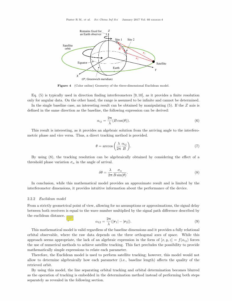
Figure 4 (Color online) Geometry of the three-dimensional Euclidean model.

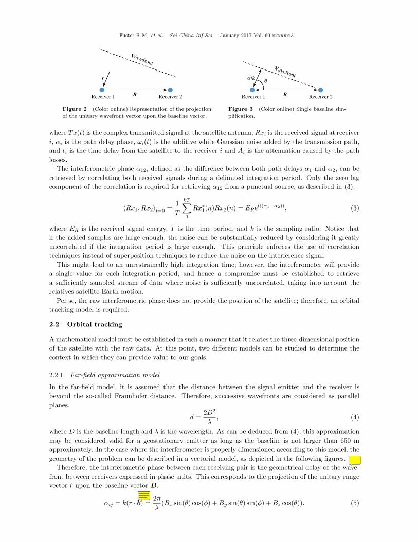
Eq. (5) is typically used in direction finding interferometers [9, 10], as it provides a finite resolution

only for angular data. On the other hand, the range is assumed to be infinite and cannot be determined.

In the single baseline case, an interesting result can be obtained by manipulating (5). If the Z axis is

defined in the same direction as the baseline, the following expression can be derived:

αij =2π

λ(B cos(θ)). (6)

This result is interesting, as it provides an algebraic solution from the arriving angle to the interfero-

metric phase and vice versa. Thus, a direct tracking method is provided.

θ = arccos

(λ

2π

αijB

). (7)

By using (8), the tracking resolution can be algebraically obtained by considering the effect of a

threshold phase variation σα in the angle of arrival.

δθ =λ

2π

σαB sin(θ)

. (8)

In conclusion, while this mathematical model provides an approximate result and is limited by the

interferometer dimensions, it provides intuitive information about the performance of the device.

2.2.2 Euclidean model

From a strictly geometrical point of view, allowing for no assumptions or approximations, the signal delay

between both receivers is equal to the wave number multiplied by the signal path difference described by

the euclidean distance.

α12 =2π

λ(|r1| − |r2|). (9)

This mathematical model is valid regardless of the baseline dimensions and it provides a fully relational

orbital observable, where the raw data depends on the three orthogonal axes of space. While this

approach seems appropriate, the lack of an algebraic expression in the form of [x, y, z] = f(αij) forces

the use of numerical methods to achieve satellite tracking. This fact precludes the possibility to provide

mathematically simple expressions to relate each parameter.

Therefore, the Euclidean model is used to perform satellite tracking; however, this model would not

allow to determine algebraically how each parameter (i.e., baseline length) affects the quality of the

retrieved orbit.

By using this model, the line separating orbital tracking and orbital determination becomes blurred

as the operation of tracking is embedded in the determination method instead of performing both steps

separately as revealed in the following section.

Fuster R M, et al. Sci China Inf Sci January 2017 Vol. 60 xxxxxx:5

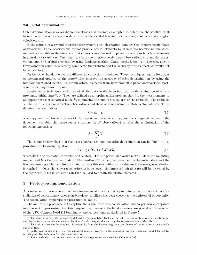
2.3 Orbit determination

Orbit determination involves different methods and techniques adopted to determine the satellite orbit

from a collection of observation data provided by orbital tracking, for instance, a set of ranges, angles,

velocities, etc.

In the context of a ground interferometer system, such observation data are the interferometric phase

observations. These observations cannot provide orbital elements by themselves because no analytical

method is available in the literature that connects interferometric phase observations to orbital elements

in a straightforward way. One may transform the interferometric phase observations into angular obser-

vations and find orbital elements by using Laplaces method, Gauss method, etc. [11]; however, such a

transformation could considerably complicate the problem and the accuracy of these methods would not

be satisfactory.

On the other hand, one can use differential correction techniques. These techniques require iterations

or incremental updates to the state1) that improve the accuracy of orbit determination by using the

methods mentioned before. To obtain orbital elements from interferometric phase observations, least-

squares techniques are proposed.

Least-squares techniques make use of all the data available to improve the determination of an ap-

proximate initial state2), x. They are defined as an optimization problem that fits the measurements to

an appropriate mathematical model3), minimizing the sum of the squares of the residuals. The residuals

will be the difference in the actual observations and those obtained using the state vector solution. Thus,

defining the residuals as

r = y0 − yc, (10)

where y0 are the observed values of the dependent variable and yc are the computed values of the

dependent variable, the least-squares criterion (for N observations) satisfies the minimization of the

following expression:

J =

N∑i=1

ri2. (11)

The complete formulation of the least-squares technique for orbit determination can be found in [11]

providing the following equation:

δx = (ATWA)−1ATWb, (12)

where δx is the estimated correction to the state, A is the partial-derivative matrix, W is the weighting

matrix, and b is the residual matrix. The resulting δx value must be added to the initial state and the

least-squares algorithm will iterate again by using this new initial state value until a convergence criterion

is reached4). Once the convergence criterion is achieved, the improved initial state will be provided by

the algorithm. This initial state can then be used to obtain the orbital elements..

3 Prototype implementation

A two-element interferometer has been implemented to carry out a preliminary test of concept. A con-

stellation of geostationary television broadcast satellites has been chosen as the emitters of opportunity.

The constellation properties are presented in Table 1.

The aim of the prototype is to capture the signal from this constellation and to perform appropriate

interferometric processing. For this purpose, two coherent Ku band receivers are placed on the rooftop

of the UPC Campus Nord D3 building at known locations, as depicted in Figure 5.

1) The state of a satellite in space is defined by six quantities that can be called either a state vector (position and

velocity vectors) or an element set (a collection of scalar magnitudes and angular representations of the orbit).2) This initial state can be obtained, for example, from the known longitude coordinates of the satellite at one specific

epoch of time.3) In the case under study, the mathematical models involved in the operation are the Euclidean model for orbital

tracking and Kepler’s laws for orbit determination.4) Some methods to determine the criterion of convergence are discussed by Vallado in [11].

Fuster R M, et al. Sci China Inf Sci January 2017 Vol. 60 xxxxxx:6

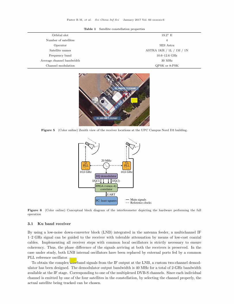
Table 1 Satellite constellation properties

Orbital slot 19.2 E

Number of satellites 4

Operator SES Astra

Satellite names ASTRA 1KR / 1L / 1M / 1N

Frequency band 10.6–12.6 GHz

Average channel bandwidth 30 MHz

Channel modulation QPSK or 8-PSK

Figure 5 (Color online) Zenith view of the receiver locations at the UPC Campus Nord D3 building.

PLL PLL

20 MHz

10,6 GHz 10,6 GHz

I/Q demodulator

I/Q(1) I/Q(2)

FPGA (virtex-4):correlator

UART

PC: least squares Main signalsReference clocks

Figure 6 (Color online) Conceptual block diagram of the interferometer depicting the hardware performing the full

operation

3.1 Ku band receiver

By using a low-noise down-converter block (LNB) integrated in the antenna feeder, a multichannel IF

1–2 GHz signal can be guided to the receiver with tolerable attenuation by means of low-cost coaxial

cables. Implementing all receiver steps with common local oscillators is strictly necessary to ensure

coherency. Thus, the phase difference of the signals arriving at both the receivers is preserved. In the

case under study, both LNB internal oscillators have been replaced by external ports fed by a common

PLL reference oscillator.

To obtain the complex baseband signals from the IF output at the LNB, a custom two-channel demod-

ulator has been designed. The demodulator output bandwidth is 40 MHz for a total of 2-GHz bandwidth

available at the IF stage. Corresponding to one of the multiplexed DVB-S channels. Since each individual

channel is emitted by one of the four satellites in the constellation, by selecting the channel properly, the

actual satellite being tracked can be chosen.

Fuster R M, et al. Sci China Inf Sci January 2017 Vol. 60 xxxxxx:7

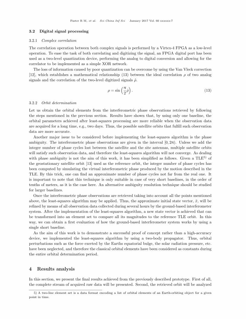
3.2 Digital signal processing

3.2.1 Complex correlation

The correlation operation between both complex signals is performed by a Virtex-4 FPGA as a low-level

operation. To ease the task of both correlating and digitizing the signal, an FPGA digital port has been

used as a two-level quantization device, performing the analog to digital conversion and allowing for the

correlator to be implemented as a simple XOR network.

The loss of information caused by poor quantization can be overcome by using the Van Vleck correction

[12], which establishes a mathematical relationship (13) between the ideal correlation ρ of two analog

signals and the correlation of the two-level digitized signals ρ.

ρ = sin(π

2ρ). (13)

3.2.2 Orbit determination

Let us obtain the orbital elements from the interferometric phase observations retrieved by following

the steps mentioned in the previous section. Results have shown that, by using only one baseline, the

orbital parameters achieved after least-squares processing are more reliable when the observation data

are acquired for a long time, e.g., two days. Thus, the possible satellite orbits that fulfill such observation

data are more accurate.

Another major issue to be considered before implementing the least-squares algorithm is the phase

ambiguity. The interferometric phase observations are given in the interval [0, 2π). Unless we add the

integer number of phase cycles lost between the satellite and the site antennas, multiple satellite orbits

will satisfy such observation data, and therefore the least-squares algorithm will not converge. As dealing

with phase ambiguity is not the aim of this work, it has been simplified as follows. Given a TLE5) of

the geostationary satellite orbit [13] used as the reference orbit, the integer number of phase cycles has

been computed by simulating the virtual interferometric phase produced by the motion described in the

TLE. By this trick, one can find an approximate number of phase cycles not far from the real one. It

is important to note that this technique is only suitable in case of very short baselines, in the order of

tenths of meters, as it is the case here. An alternative ambiguity resolution technique should be studied

for larger baselines.

Once the interferometric phase observations are retrieved taking into account all the points mentioned

above, the least-squares algorithm may be applied. Thus, the approximate initial state vector, x, will be

refined by means of all observation data collected during several hours by the ground-based interferometer

system. After the implementation of the least-squares algorithm, a new state vector is achieved that can

be transformed into an element set to compare all its magnitudes to the reference TLE orbit. In this

way, we can obtain a first evaluation of how the ground-based interferometer system works by using a

single short baseline.

As the aim of this work is to demonstrate a successful proof of concept rather than a high-accuracy

device, we implemented the least-squares algorithm by using a two-body propagator. Thus, orbital

perturbations such as the force exerted by the Earths equatorial bulge, the solar radiation pressure, etc.

have been neglected, and therefore the classical orbital elements have been considered as constants during

the entire orbital determination period.

4 Results analysis

In this section, we present the final results achieved from the previously described prototype. First of all,

the complete stream of acquired raw data will be presented. Second, the retrieved orbit will be analyzed

5) A two-line element set is a data format encoding a list of orbital elements of an Earth-orbiting object for a given

point in time.

Fuster R M, et al. Sci China Inf Sci January 2017 Vol. 60 xxxxxx:8

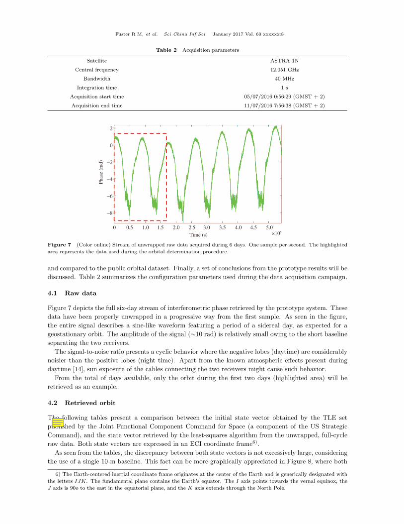
Table 2 Acquisition parameters

Satellite ASTRA 1N

Central frequency 12.051 GHz

Bandwidth 40 MHz

Integration time 1 s

Acquisition start time 05/07/2016 0:56:29 (GMST + 2)

Acquisition end time 11/07/2016 7:56:38 (GMST + 2)P

hase

(ra

d)

2

0

−2

−4

−6

−8

0 0.5 1.0 1.5 2.0 2.5 3.0 3.5 4.0 4.5 5.0

×105Time (s)

Figure 7 (Color online) Stream of unwrapped raw data acquired during 6 days. One sample per second. The highlighted

area represents the data used during the orbital determination procedure.

and compared to the public orbital dataset. Finally, a set of conclusions from the prototype results will be

discussed. Table 2 summarizes the configuration parameters used during the data acquisition campaign.

4.1 Raw data

Figure 7 depicts the full six-day stream of interferometric phase retrieved by the prototype system. These

data have been properly unwrapped in a progressive way from the first sample. As seen in the figure,

the entire signal describes a sine-like waveform featuring a period of a sidereal day, as expected for a

geostationary orbit. The amplitude of the signal (∼10 rad) is relatively small owing to the short baseline

separating the two receivers.

The signal-to-noise ratio presents a cyclic behavior where the negative lobes (daytime) are considerably

noisier than the positive lobes (night time). Apart from the known atmospheric effects present during

daytime [14], sun exposure of the cables connecting the two receivers might cause such behavior.

From the total of days available, only the orbit during the first two days (highlighted area) will be

retrieved as an example.

4.2 Retrieved orbit

The following tables present a comparison between the initial state vector obtained by the TLE set

published by the Joint Functional Component Command for Space (a component of the US Strategic

Command), and the state vector retrieved by the least-squares algorithm from the unwrapped, full-cycle

raw data. Both state vectors are expressed in an ECI coordinate frame6).

As seen from the tables, the discrepancy between both state vectors is not excessively large, considering

the use of a single 10-m baseline. This fact can be more graphically appreciated in Figure 8, where both

6) The Earth-centered inertial coordinate frame originates at the center of the Earth and is generically designated with

the letters IJK. The fundamental plane contains the Earth’s equator. The I axis points towards the vernal equinox, the

J axis is 90o to the east in the equatorial plane, and the K axis extends through the North Pole.

Fuster R M, et al. Sci China Inf Sci January 2017 Vol. 60 xxxxxx:9

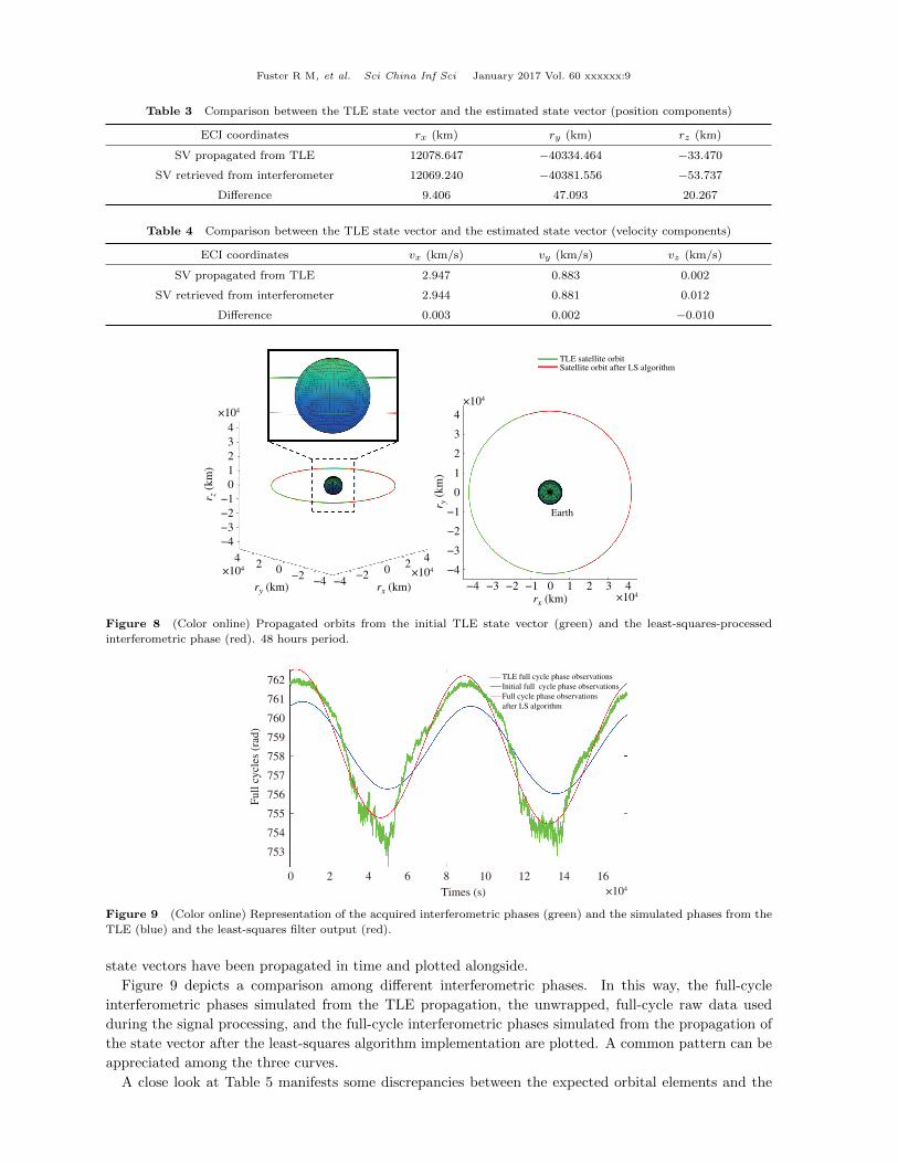
Table 3 Comparison between the TLE state vector and the estimated state vector (position components)

ECI coordinates rx (km) ry (km) rz (km)

SV propagated from TLE 12078.647 −40334.464 −33.470

SV retrieved from interferometer 12069.240 −40381.556 −53.737

Difference 9.406 47.093 20.267

Table 4 Comparison between the TLE state vector and the estimated state vector (velocity components)

ECI coordinates vx (km/s) vy (km/s) vz (km/s)

SV propagated from TLE 2.947 0.883 0.002

SV retrieved from interferometer 2.944 0.881 0.012

Difference 0.003 0.002 −0.010

TLE satellite orbitSatellite orbit after LS algorithm

4

3

2

1

0

−1

−2

−3

−4

r z (

km

)

ry (km) rx (km)

×104

×104

42

0−4

−2

42

0−4

−2

Earth

r y (

km

)

4

3

2

1

0

−1

−2

−3

−4

×104

rx (km) ×104−4 −3 −2 −1 0 1 2 3 4

×104

Figure 8 (Color online) Propagated orbits from the initial TLE state vector (green) and the least-squares-processed

interferometric phase (red). 48 hours period.

TLE full cycle phase observations

Initial full cycle phase observations

Full cycle phase observations

after LS algorithm

Full

cycl

es (

rad)

762

761

760

759

758

757

756

755

754

753

0 2 4 6 8 10 12 14 16

×104Times (s)

Figure 9 (Color online) Representation of the acquired interferometric phases (green) and the simulated phases from the

TLE (blue) and the least-squares filter output (red).

state vectors have been propagated in time and plotted alongside.

Figure 9 depicts a comparison among different interferometric phases. In this way, the full-cycle

interferometric phases simulated from the TLE propagation, the unwrapped, full-cycle raw data used

during the signal processing, and the full-cycle interferometric phases simulated from the propagation of

the state vector after the least-squares algorithm implementation are plotted. A common pattern can be

appreciated among the three curves.

A close look at Table 5 manifests some discrepancies between the expected orbital elements and the

Fuster R M, et al. Sci China Inf Sci January 2017 Vol. 60 xxxxxx:10

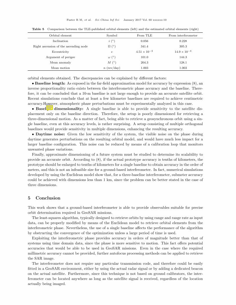
Table 5 Comparison between the TLE-published orbital elements (left) and the estimated orbital elements (right)

Orbital element Symbol From TLE From interferometer

Inclination i () 0.056 0.228

Right ascension of the ascending node Ω () 341.4 305.3

Eccentricity e 4.51 × 10−4 14.9 × 10−4

Argument of perigee ω () 101.0 144.3

Mean anomaly M () 204.3 128.1

Mean motion n (rev/day) 1.003 1.003

orbital elements obtained. The discrepancies can be explained by different factors:

• Baseline length: As exposed in the far-field approximation model for accuracy by expression (8), an

inverse proportionality ratio exists between the interferometric phase accuracy and the baseline. There-

fore, it can be concluded that a 10-m baseline is not large enough to provide an accurate satellite orbit.

Recent simulations conclude that at least a few kilometer baselines are required to achieve centimetric

accuracy.However, atmospheric phase perturbations must be experimentally analyzed in this case.

• Baseline dimensionality: A single baseline is able to provide sensitivity to the satellite dis-

placement only on the baseline direction. Therefore, the setup is poorly dimensioned for retrieving a

three-dimensional motion. As a matter of fact, being able to retrieve a geosynchronous orbit using a sin-

gle baseline, even at this accuracy levels, is rather surprising. A setup consisting of multiple orthogonal

baselines would provide sensitivity in multiple dimensions, enhancing the resulting accuracy.

• Daytime noise: Given the low sensitivity of the system, the visible noise on the phase during

daytime generates perturbations on the resulting orbital model, and would have much less impact for a

larger baseline configuration. This noise can be reduced by means of a calibration loop that monitors

unwanted phase variations.

Finally, approximate dimensioning of a future system must be studied to determine its scalability to

provide an accurate orbit. According to (8), if the actual prototype accuracy is tenths of kilometers, the

prototype should be enlarged to tenths of kilometers for a single baseline to obtain accuracy in the order of

meters, and this is not an infeasible size for a ground-based interferometer. In fact, numerical simulations

developed by using the Euclidean model show that, for a three-baseline interferometer, submeter accuracy

could be achieved with dimensions less than 1 km, since the problem can be better stated in the case of

three dimensions.

5 Conclusion

This work shows that a ground-based interferometer is able to provide observables suitable for precise

orbit determination required in GeoSAR missions.

The least-squares algorithm, typically designed to retrieve orbits by using range and range rate as input

data, can be properly modified by means of the Euclidean model to retrieve orbital elements from the

interferometric phase. Nevertheless, the use of a single baseline affects the performance of the algorithm

by obstructing the convergence of the optimization unless a large period of time is used.

Exploiting the interferometric phase provides accuracy in orders of magnitude better than that of

systems using time domain data, since the phase is more sensitive to motion. This fact offers potential

accuracies that would be able to be used in GeoSAR missions. Even in the case where the required

millimetric accuracy cannot be provided, further autofocus processing methods can be applied to retrieve

the SAR image.

The interferometer does not require any particular transmission code, and therefore could be easily

fitted in a GeoSAR environment, either by using the actual radar signal or by adding a dedicated beacon

on the actual satellite. Furthermore, since this technique is not based on ground calibrators, the inter-

ferometer can be located anywhere as long as the satellite signal is received, regardless of the location

actually being imaged.

Fuster R M, et al. Sci China Inf Sci January 2017 Vol. 60 xxxxxx:11

This prototype will be enhanced in the near future on the basis of upgrades suggested for this work.

Acknowledgements This work has been financed by the Spanish Science, Research and Innovation Plan

(MINECO) with Project Code TIN2014-55413-C2-1-P.

Conflict of interest The authors declare that they have no conflict of interest.

References

1 Hu C, Long T, Zeng T, et al. The accurate focusing and resolution analysis method in geosynchronous SAR. IEEE

Trans Geosci Remote Sens, 2011, 49: 3548–3563

2 Ruiz-Rodon J, Broquetas A, Makhoul E, et al. Nearly zero inclination geosynchronous SAR mission analysis with long

integration time for Earth observation. IEEE Trans Geosci Remote Sens, 2014, 52: 6379–6391

3 Monti Guarnieri A, Hu C. Geosynchronous and geostationary SAR: face to face comparison. In: Proceedings of 11th

European Conference on Synthetic Aperture Radar, Hamburg, 2016. 1–4

4 Ruiz-Rodon J, Broquetas A, Monti Guarnieri A, et al. Geosyncrhonous SAR focusing with atmospheric phase screen

retrieval and compensation. IEEE Trans Geosci Remote Sens, 2013, 51: 4397–4404

5 Hu C, Li Y H, Dong X C, et al. Performance analysis of L-band geosynchronous SAR imaging in the presence of

ionospheric scintillation. IEEE Trans Geosci Remote Sens, 2017, 55: 159–172

6 Martin Fuster R, Fernandez Uson M, Casado Blanco D, et al. Proposed satellite position determination systems and

techniques for Geostationary Synthetic Aperture Radar. Eur J Remot Sens, 2016, 49: 735–744

7 Lengyel B A. A Michelson-type interferometer for microwave measurements. Proc IRE, 1949, 37: 1242–1244

8 Holler C M, Jones M E, Taylor A C, et al. A 220-GHz analog lag correlator for radio interferometry. IEEE Trans

Instrum Meas, 2012, 61: 2253–2261

9 Qin L, Jia K X, He Z S. Performance analysis of correlative interferometer direction finder using cosine function.

In: Proceedings of International Symposium on Intelligent Signal Processing and Communication Systems, Chengdu,

2010. 1–4

10 Duncan J W. The effect of ground reflections and scattering on an interferometer direction finder. IEEE Trans Aerosp

Electron Syst, 1967, AES-3: 922–932

11 Vallado D A. Fundamentals of Astrodynamics and Applications. Hawthorne: Microcosm Press, 2013

12 Van Vleck J H, Middleton D. The spectrum of clipped noise. Proc IEEE, 1966, 54: 2–19

13 National Aeronautics and Space Administration. Definition of two-line element set coordinate system. http:

//spaceflight.nasa.gov/realdata/sightings/SSapplications/Post/JavaSSOP/SSOP Help/tle def.html

14 Morabito D D, D’Addario L R, Acosta R J, et al. Tropospheric delay statistics measured by two site test interferometers

at Goldstone, California. Radio Sci, 2013, 48: 729–738