116
Interior-Point Methods for Nonlinear Programming Robert Vanderbei July 1, 2001 Erice Operations Research and Financial Engineering, Princeton University http://www.princeton.edu/∼rvdb

Interior-Point Methodsfor Nonlinear Programming
Robert Vanderbei
July 1, 2001
Erice
Operations Research and Financial Engineering, Princeton University
http://www.princeton.edu/∼rvdb

1 Acknowledgements
• Newton
• Lagrange
• Fiacco, McCormick
• Karmarkar
• Megiddo
• Gay
• Conn, Gould, Toint, Bongartz
• Shanno, Benson

1 Acknowledgements
• Newton
• Lagrange
• Fiacco, McCormick
• Karmarkar
• Megiddo
• Gay
• Conn, Gould, Toint, Bongartz
• Shanno, Benson

1 Acknowledgements
• Newton
• Lagrange
• Fiacco, McCormick
• Karmarkar
• Megiddo
• Gay
• Conn, Gould, Toint, Bongartz
• Shanno, Benson

1 Acknowledgements
• Newton
• Lagrange
• Fiacco, McCormick
• Karmarkar
• Megiddo
• Gay
• Conn, Gould, Toint, Bongartz
• Shanno, Benson

1 Acknowledgements
• Newton
• Lagrange
• Fiacco, McCormick
• Karmarkar
• Megiddo
• Gay
• Conn, Gould, Toint, Bongartz
• Shanno, Benson

1 Acknowledgements
• Newton
• Lagrange
• Fiacco, McCormick
• Karmarkar
• Megiddo
• Gay
• Conn, Gould, Toint, Bongartz
• Shanno, Benson

1 Acknowledgements
• Newton
• Lagrange
• Fiacco, McCormick
• Karmarkar
• Megiddo
• Gay
• Conn, Gould, Toint, Bongartz
• Shanno, Benson

1 Acknowledgements
• Newton
• Lagrange
• Fiacco, McCormick
• Karmarkar
• Megiddo
• Gay
• Conn, Gould, Toint, Bongartz
• Shanno, Benson

1 Acknowledgements
• Newton
• Lagrange
• Fiacco, McCormick
• Karmarkar
• Megiddo
• Gay
• Conn, Gould, Toint, Bongartz
• Shanno, Benson

2 Outline
• Algorithm
– Basic Paradigm
– Step-Length Control
– Diagonal Perturbation
– Jamming
– Free Variables
• Some Applications
– Celestial Mechanics
– Putting on an Uneven Green
– Goddard Rocket Problem
2 Outline
• Algorithm
– Basic Paradigm
– Step-Length Control
– Diagonal Perturbation
– Jamming
– Free Variables
• Some Applications
– Celestial Mechanics
– Putting on an Uneven Green
– Goddard Rocket Problem

2 Outline
• Algorithm
– Basic Paradigm
– Step-Length Control
– Diagonal Perturbation
– Jamming
– Free Variables
• Some Applications
– Celestial Mechanics
– Putting on an Uneven Green
– Goddard Rocket Problem

2 Outline
• Algorithm
– Basic Paradigm
– Step-Length Control
– Diagonal Perturbation
– Jamming
– Free Variables
• Some Applications
– Celestial Mechanics
– Putting on an Uneven Green
– Goddard Rocket Problem

2 Outline
• Algorithm
– Basic Paradigm
– Step-Length Control
– Diagonal Perturbation
– Jamming
– Free Variables
• Some Applications
– Celestial Mechanics
– Putting on an Uneven Green
– Goddard Rocket Problem

2 Outline
• Algorithm
– Basic Paradigm
– Step-Length Control
– Diagonal Perturbation
– Jamming
– Free Variables
• Some Applications
– Celestial Mechanics
– Putting on an Uneven Green
– Goddard Rocket Problem

2 Outline
• Algorithm
– Basic Paradigm
– Step-Length Control
– Diagonal Perturbation
– Jamming
– Free Variables
• Some Applications
– Celestial Mechanics
– Putting on an Uneven Green
– Goddard Rocket Problem
2 Outline
• Algorithm
– Basic Paradigm
– Step-Length Control
– Diagonal Perturbation
– Jamming
– Free Variables
• Some Applications
– Celestial Mechanics
– Putting on an Uneven Green
– Goddard Rocket Problem

2 Outline
• Algorithm
– Basic Paradigm
– Step-Length Control
– Diagonal Perturbation
– Jamming
– Free Variables
• Some Applications
– Celestial Mechanics
– Putting on an Uneven Green
– Goddard Rocket Problem
2 Outline
• Algorithm
– Basic Paradigm
– Step-Length Control
– Diagonal Perturbation
– Jamming
– Free Variables
• Some Applications
– Celestial Mechanics
– Putting on an Uneven Green
– Goddard Rocket Problem

2 Outline
• Algorithm
– Basic Paradigm
– Step-Length Control
– Diagonal Perturbation
– Jamming
– Free Variables
• Some Applications
– Celestial Mechanics
– Putting on an Uneven Green
– Goddard Rocket Problem

The Interior-Point Algorithm

3 Introduce Slack Variables
• Start with an optimization problem—for now, the simplest NLP:
minimize f(x)
subject to hi(x) ≥ 0, i = 1, . . . , m
• Introduce slack variables to make all inequality constraints into nonnegativities:
minimize f(x)
subject to h(x) − w = 0,
w ≥ 0

3 Introduce Slack Variables
• Start with an optimization problem—for now, the simplest NLP:
minimize f(x)
subject to hi(x) ≥ 0, i = 1, . . . , m
• Introduce slack variables to make all inequality constraints into nonnegativities:
minimize f(x)
subject to h(x) − w = 0,
w ≥ 0

3 Introduce Slack Variables
• Start with an optimization problem—for now, the simplest NLP:
minimize f(x)
subject to hi(x) ≥ 0, i = 1, . . . , m
• Introduce slack variables to make all inequality constraints into nonnegativities:
minimize f(x)
subject to h(x) − w = 0,
w ≥ 0
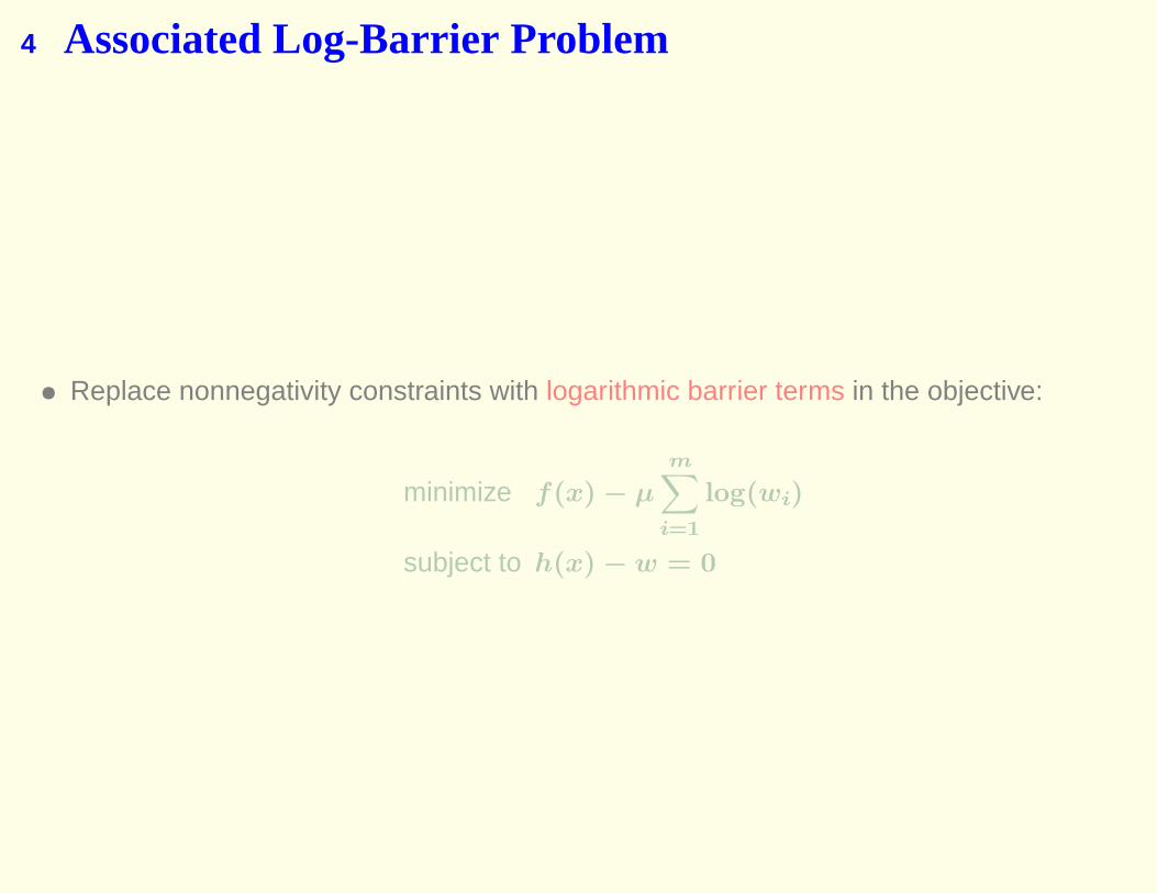
4 Associated Log-Barrier Problem
• Replace nonnegativity constraints with logarithmic barrier terms in the objective:
minimize f(x) − µ
m∑i=1
log(wi)
subject to h(x) − w = 0

4 Associated Log-Barrier Problem
• Replace nonnegativity constraints with logarithmic barrier terms in the objective:
minimize f(x) − µ
m∑i=1
log(wi)
subject to h(x) − w = 0

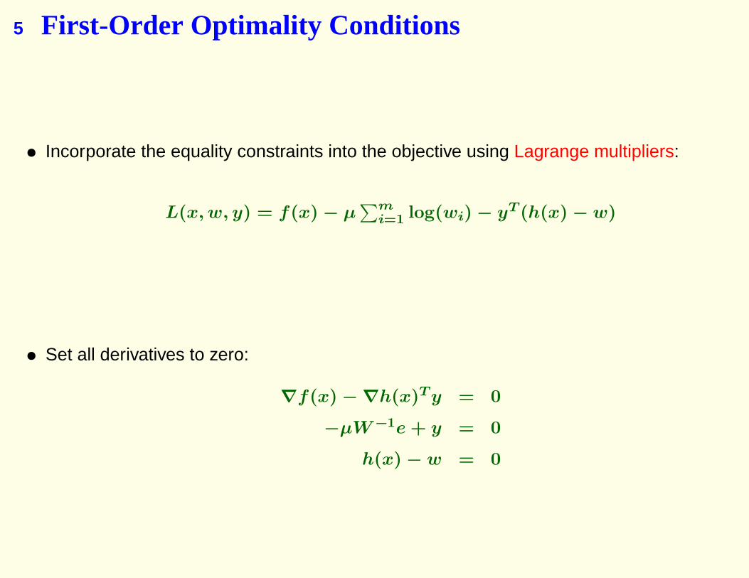
5 First-Order Optimality Conditions
• Incorporate the equality constraints into the objective using Lagrange multipliers:
L(x, w, y) = f(x) − µ∑m
i=1 log(wi) − yT (h(x) − w)
• Set all derivatives to zero:
∇f(x) − ∇h(x)T y = 0
−µW −1e + y = 0
h(x) − w = 0

5 First-Order Optimality Conditions
• Incorporate the equality constraints into the objective using Lagrange multipliers:
L(x, w, y) = f(x) − µ∑m
i=1 log(wi) − yT (h(x) − w)
• Set all derivatives to zero:
∇f(x) − ∇h(x)T y = 0
−µW −1e + y = 0
h(x) − w = 0
5 First-Order Optimality Conditions
• Incorporate the equality constraints into the objective using Lagrange multipliers:
L(x, w, y) = f(x) − µ∑m
i=1 log(wi) − yT (h(x) − w)
• Set all derivatives to zero:
∇f(x) − ∇h(x)T y = 0
−µW −1e + y = 0
h(x) − w = 0

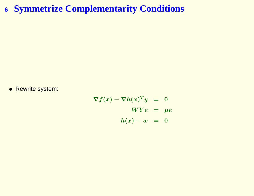
6 Symmetrize Complementarity Conditions
• Rewrite system:
∇f(x) − ∇h(x)T y = 0
WY e = µe
h(x) − w = 0
6 Symmetrize Complementarity Conditions
• Rewrite system:
∇f(x) − ∇h(x)T y = 0
WY e = µe
h(x) − w = 0

7 Apply Newton’s Method
• Apply Newton’s method to compute search directions, ∆x, ∆w, ∆y:
H(x, y) 0 −A(x)T
0 Y W
A(x) −I 0
∆x
∆w
∆y
=
−∇f(x) + A(x)T y
µe − WY e
−h(x) + w
.
Here,
H(x, y) = ∇2f(x) −∑m
i=1 yi∇2hi(x)
and
A(x) = ∇h(x)
• Note: H(x, y) is positive semidefinite if f is convex, each hi is concave, and each
yi ≥ 0.
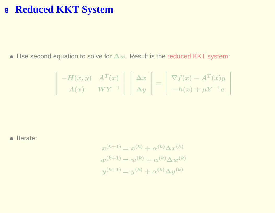
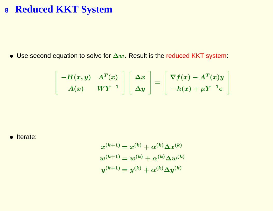
8 Reduced KKT System
• Use second equation to solve for ∆w. Result is the reduced KKT system:
−H(x, y) AT (x)
A(x) WY −1
∆x
∆y
=
∇f(x) − AT (x)y
−h(x) + µY −1e
• Iterate:
x(k+1) = x(k) + α(k)∆x(k)
w(k+1) = w(k) + α(k)∆w(k)
y(k+1) = y(k) + α(k)∆y(k)

8 Reduced KKT System
• Use second equation to solve for ∆w. Result is the reduced KKT system:
−H(x, y) AT (x)
A(x) WY −1
∆x
∆y
=
∇f(x) − AT (x)y
−h(x) + µY −1e
• Iterate:
x(k+1) = x(k) + α(k)∆x(k)
w(k+1) = w(k) + α(k)∆w(k)
y(k+1) = y(k) + α(k)∆y(k)
8 Reduced KKT System
• Use second equation to solve for ∆w. Result is the reduced KKT system:
−H(x, y) AT (x)
A(x) WY −1
∆x
∆y
=
∇f(x) − AT (x)y
−h(x) + µY −1e
• Iterate:
x(k+1) = x(k) + α(k)∆x(k)
w(k+1) = w(k) + α(k)∆w(k)
y(k+1) = y(k) + α(k)∆y(k)

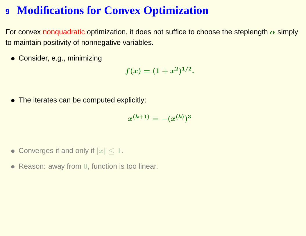
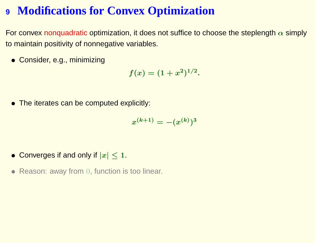
9 Modifications for Convex Optimization
For convex nonquadratic optimization, it does not suffice to choose the steplength α simply
to maintain positivity of nonnegative variables.
• Consider, e.g., minimizing
f(x) = (1 + x2)1/2.
• The iterates can be computed explicitly:
x(k+1) = −(x(k))3
• Converges if and only if |x| ≤ 1.
• Reason: away from 0, function is too linear.

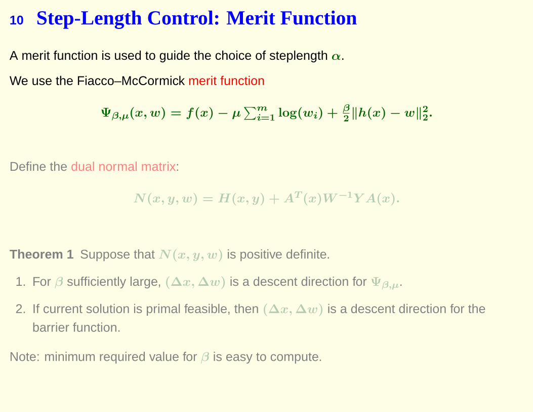
10 Step-Length Control: Merit Function
A merit function is used to guide the choice of steplength α.
We use the Fiacco–McCormick merit function
Ψβ,µ(x, w) = f(x) − µ∑m
i=1 log(wi) + β2‖h(x) − w‖2
2.
Define the dual normal matrix:
N(x, y, w) = H(x, y) + AT (x)W −1Y A(x).
Theorem 1 Suppose that N(x, y, w) is positive definite.
1. For β sufficiently large, (∆x, ∆w) is a descent direction for Ψβ,µ.
2. If current solution is primal feasible, then (∆x, ∆w) is a descent direction for the
barrier function.
Note: minimum required value for β is easy to compute.
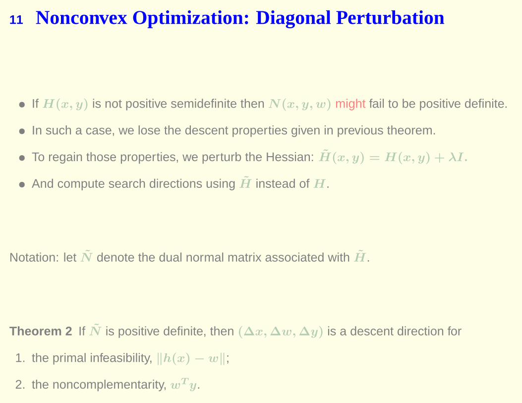
11 Nonconvex Optimization: Diagonal Perturbation
• If H(x, y) is not positive semidefinite then N(x, y, w) might fail to be positive definite.
• In such a case, we lose the descent properties given in previous theorem.
• To regain those properties, we perturb the Hessian: H(x, y) = H(x, y) + λI.
• And compute search directions using H instead of H.
Notation: let N denote the dual normal matrix associated with H.
Theorem 2 If N is positive definite, then (∆x, ∆w, ∆y) is a descent direction for
1. the primal infeasibility, ‖h(x) − w‖;
2. the noncomplementarity, wT y.
12 Notes:
• Not necessarily a descent direction for dual infeasibility.
• A line search is performed to find a value of λ within a factor of 2 of the smallest
permissible value.
12 Notes:
• Not necessarily a descent direction for dual infeasibility.
• A line search is performed to find a value of λ within a factor of 2 of the smallest
permissible value.

12 Notes:
• Not necessarily a descent direction for dual infeasibility.
• A line search is performed to find a value of λ within a factor of 2 of the smallest
permissible value.

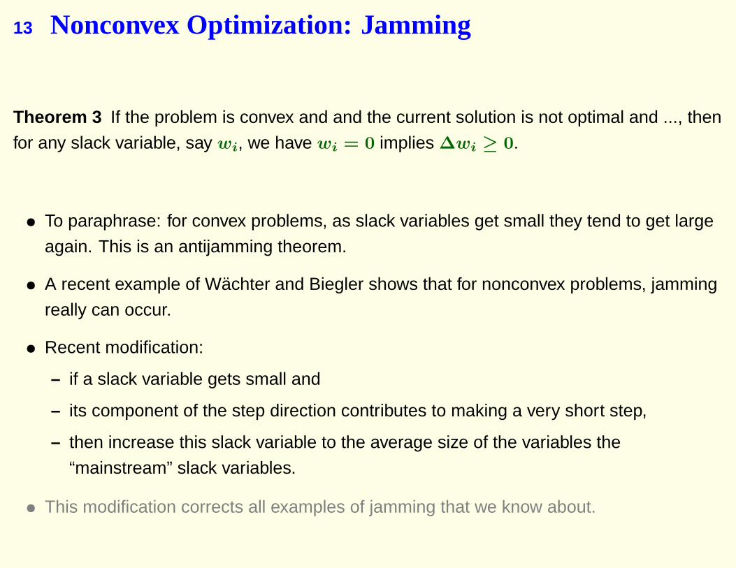
13 Nonconvex Optimization: Jamming
Theorem 3 If the problem is convex and and the current solution is not optimal and ..., then
for any slack variable, say wi, we have wi = 0 implies ∆wi ≥ 0.
• To paraphrase: for convex problems, as slack variables get small they tend to get large
again. This is an antijamming theorem.
• A recent example of Wachter and Biegler shows that for nonconvex problems, jamming
really can occur.
• Recent modification:
– if a slack variable gets small and
– its component of the step direction contributes to making a very short step,
– then increase this slack variable to the average size of the variables the
“mainstream” slack variables.
• This modification corrects all examples of jamming that we know about.

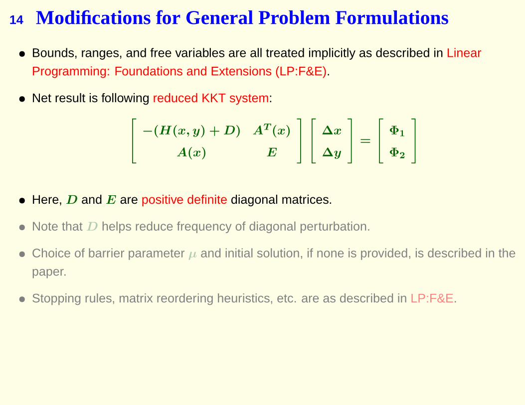
14 Modifications for General Problem Formulations
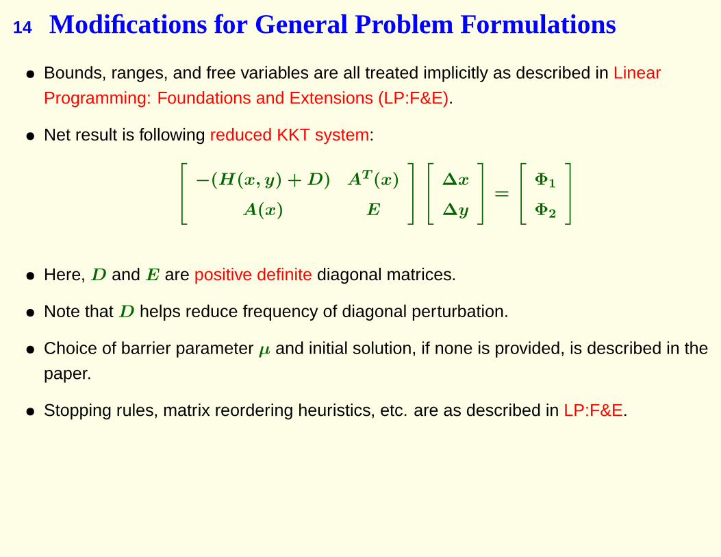
• Bounds, ranges, and free variables are all treated implicitly as described in Linear
Programming: Foundations and Extensions (LP:F&E).
• Net result is following reduced KKT system: −(H(x, y) + D) AT (x)
A(x) E
∆x
∆y
=
Φ1
Φ2
• Here, D and E are positive definite diagonal matrices.
• Note that D helps reduce frequency of diagonal perturbation.
• Choice of barrier parameter µ and initial solution, if none is provided, is described in the
paper.
• Stopping rules, matrix reordering heuristics, etc. are as described in LP:F&E.

14 Modifications for General Problem Formulations
• Bounds, ranges, and free variables are all treated implicitly as described in Linear
Programming: Foundations and Extensions (LP:F&E).
• Net result is following reduced KKT system: −(H(x, y) + D) AT (x)
A(x) E
∆x
∆y
=
Φ1
Φ2
• Here, D and E are positive definite diagonal matrices.
• Note that D helps reduce frequency of diagonal perturbation.
• Choice of barrier parameter µ and initial solution, if none is provided, is described in the
paper.
• Stopping rules, matrix reordering heuristics, etc. are as described in LP:F&E.

15 Focus of Free Variables
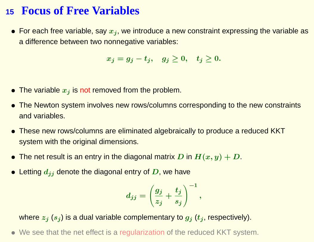
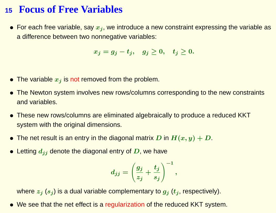
• For each free variable, say xj , we introduce a new constraint expressing the variable asa difference between two nonnegative variables:
xj = gj − tj, gj ≥ 0, tj ≥ 0.
• The variable xj is not removed from the problem.
• The Newton system involves new rows/columns corresponding to the new constraintsand variables.
• These new rows/columns are eliminated algebraically to produce a reduced KKTsystem with the original dimensions.
• The net result is an entry in the diagonal matrix D in H(x, y) + D.
• Letting djj denote the diagonal entry of D, we have
djj =
(gj
zj+
tj
sj
)−1
,
where zj (sj) is a dual variable complementary to gj (tj , respectively).
• We see that the net effect is a regularization of the reduced KKT system.

15 Focus of Free Variables
• For each free variable, say xj , we introduce a new constraint expressing the variable asa difference between two nonnegative variables:
xj = gj − tj, gj ≥ 0, tj ≥ 0.
• The variable xj is not removed from the problem.
• The Newton system involves new rows/columns corresponding to the new constraintsand variables.
• These new rows/columns are eliminated algebraically to produce a reduced KKTsystem with the original dimensions.
• The net result is an entry in the diagonal matrix D in H(x, y) + D.
• Letting djj denote the diagonal entry of D, we have
djj =
(gj
zj+
tj
sj
)−1
,
where zj (sj) is a dual variable complementary to gj (tj , respectively).
• We see that the net effect is a regularization of the reduced KKT system.

Some Applications

16 Celestial Mechanics—Periodic Orbits
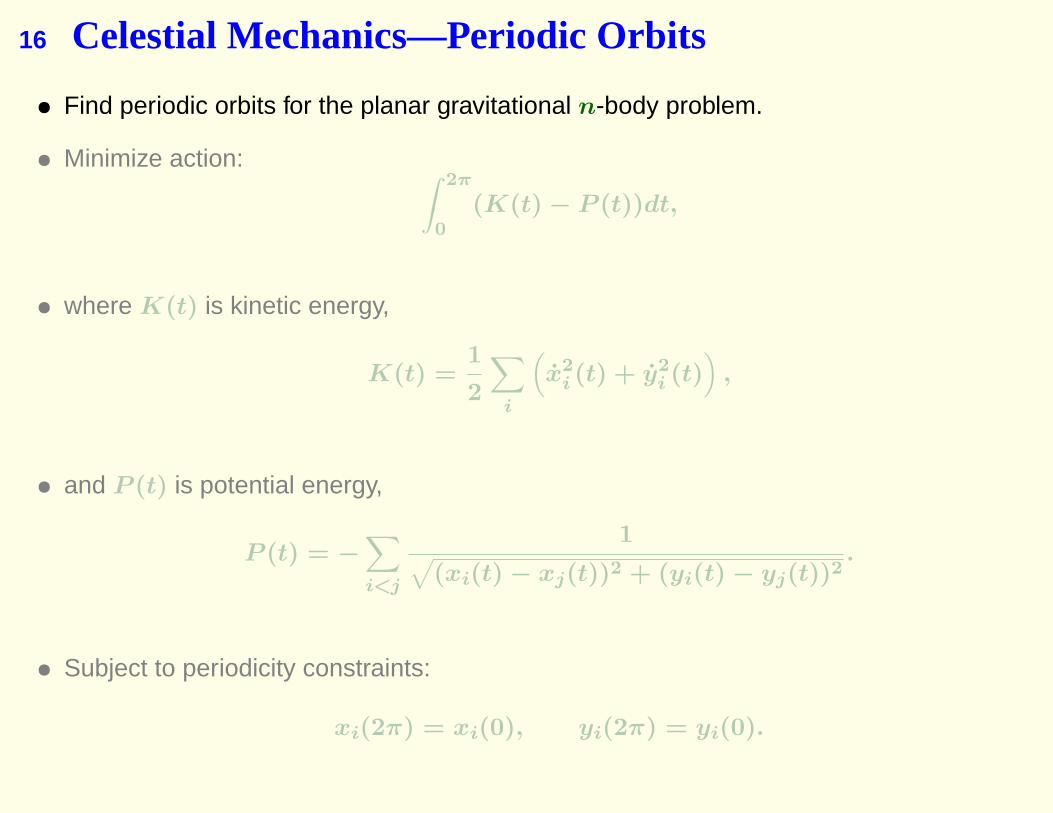
• Find periodic orbits for the planar gravitational n-body problem.
• Minimize action: ∫ 2π
0(K(t) − P (t))dt,
• where K(t) is kinetic energy,
K(t) =1
2
∑i
(x2
i (t) + y2i (t)
),
• and P (t) is potential energy,
P (t) = −∑i<j
1√(xi(t) − xj(t))2 + (yi(t) − yj(t))2
.
• Subject to periodicity constraints:
xi(2π) = xi(0), yi(2π) = yi(0).
16 Celestial Mechanics—Periodic Orbits
• Find periodic orbits for the planar gravitational n-body problem.
• Minimize action: ∫ 2π
0(K(t) − P (t))dt,
• where K(t) is kinetic energy,
K(t) =1
2
∑i
(x2
i (t) + y2i (t)
),
• and P (t) is potential energy,
P (t) = −∑i<j
1√(xi(t) − xj(t))2 + (yi(t) − yj(t))2
.
• Subject to periodicity constraints:
xi(2π) = xi(0), yi(2π) = yi(0).

17 Specific Example
Orbits.mod with n = 3 and (0, 2π) discretized into a 160 pieces gives the following results:
constraints 0
variables 960
time (secs)
LOQO 1.1
LANCELOT 8.7
SNOPT 287 (no change for last 80% of iterations)
-1.5
-1
-0.5
0
0.5
1
1.5
-1.5 -1 -0.5 0 0.5 1 1.5
"after.out"

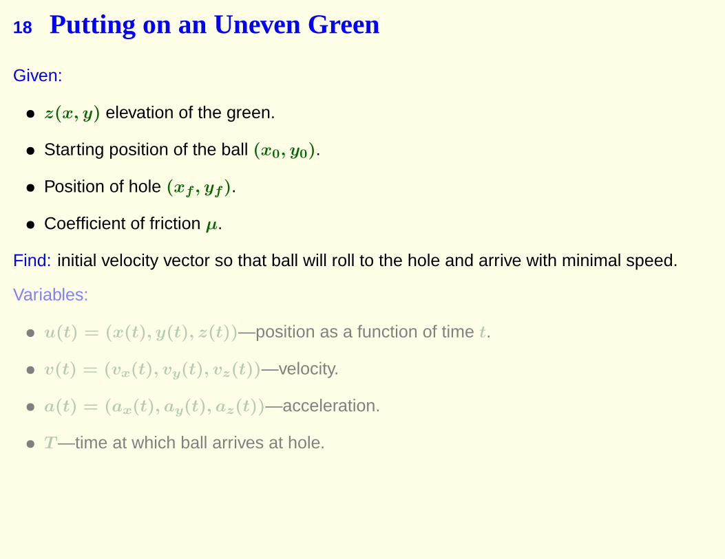
18 Putting on an Uneven Green
Given:
• z(x, y) elevation of the green.
• Starting position of the ball (x0, y0).
• Position of hole (xf , yf).
• Coefficient of friction µ.
Find: initial velocity vector so that ball will roll to the hole and arrive with minimal speed.
Variables:
• u(t) = (x(t), y(t), z(t))—position as a function of time t.
• v(t) = (vx(t), vy(t), vz(t))—velocity.
• a(t) = (ax(t), ay(t), az(t))—acceleration.
• T —time at which ball arrives at hole.

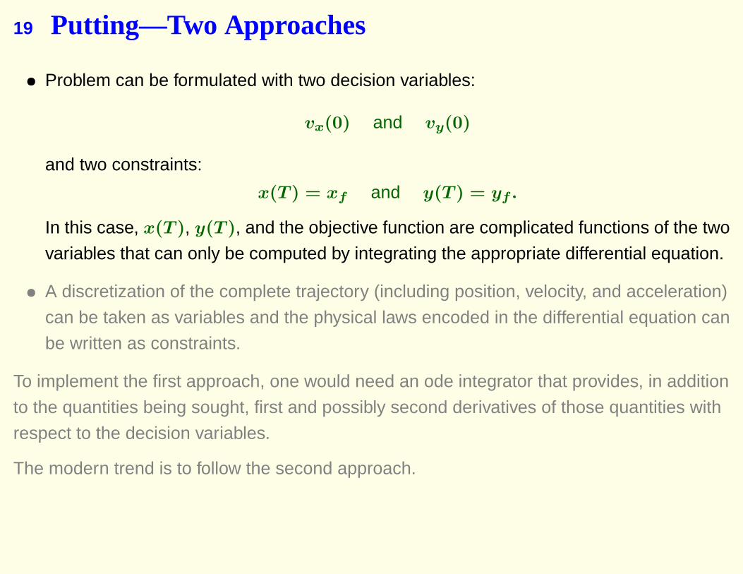
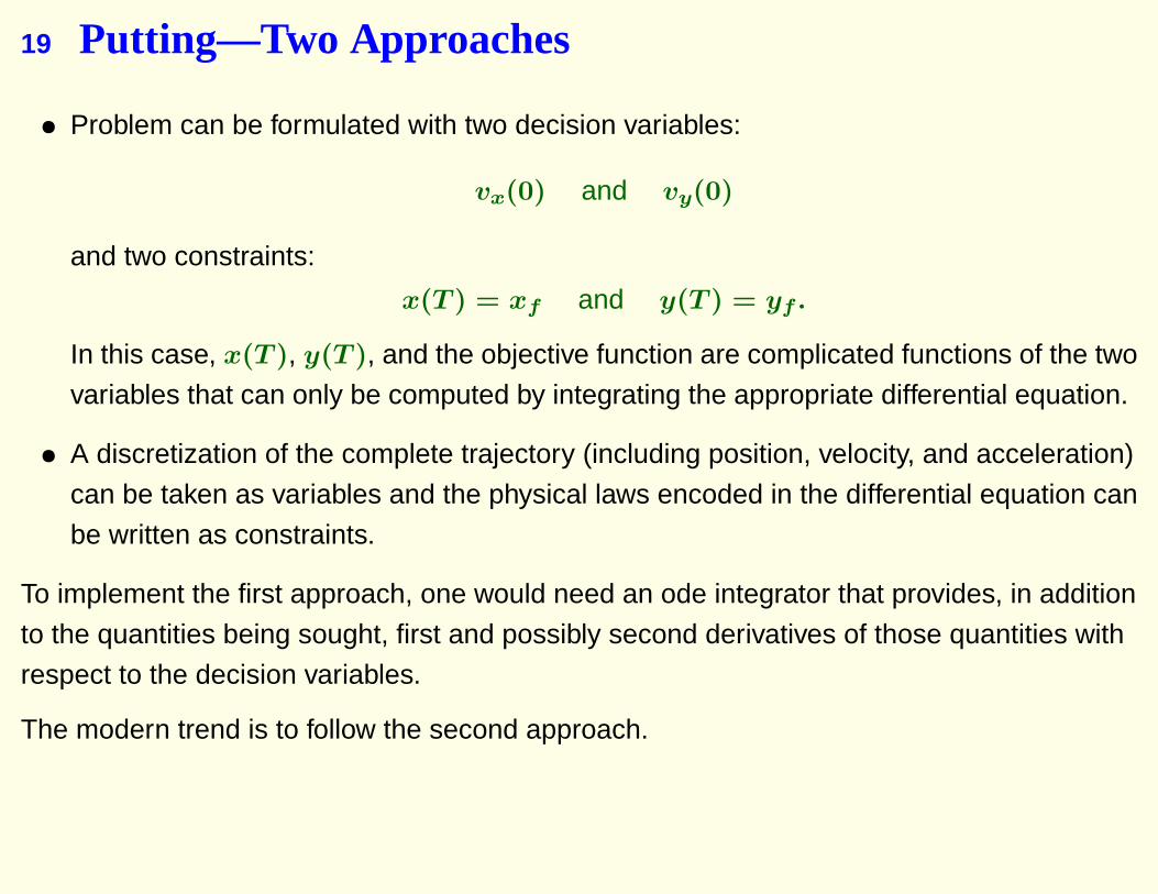
19 Putting—Two Approaches
• Problem can be formulated with two decision variables:
vx(0) and vy(0)
and two constraints:
x(T ) = xf and y(T ) = yf .
In this case, x(T ), y(T ), and the objective function are complicated functions of the two
variables that can only be computed by integrating the appropriate differential equation.
• A discretization of the complete trajectory (including position, velocity, and acceleration)
can be taken as variables and the physical laws encoded in the differential equation can
be written as constraints.
To implement the first approach, one would need an ode integrator that provides, in addition
to the quantities being sought, first and possibly second derivatives of those quantities with
respect to the decision variables.
The modern trend is to follow the second approach.

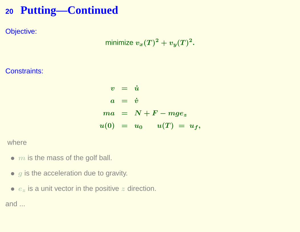
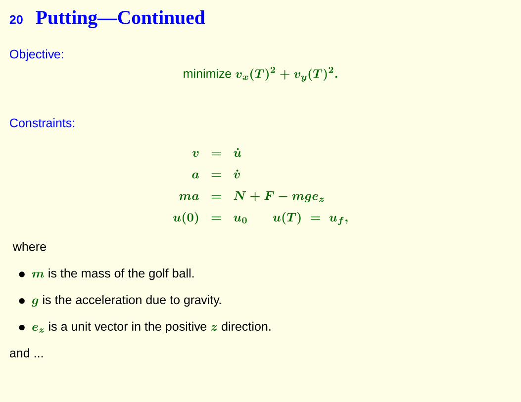
20 Putting—Continued
Objective:
minimize vx(T )2 + vy(T )2.
Constraints:
v = u
a = v
ma = N + F − mgez
u(0) = u0 u(T ) = uf ,
where
• m is the mass of the golf ball.
• g is the acceleration due to gravity.
• ez is a unit vector in the positive z direction.
and ...

20 Putting—Continued
Objective:
minimize vx(T )2 + vy(T )2.
Constraints:
v = u
a = v
ma = N + F − mgez
u(0) = u0 u(T ) = uf ,
where
• m is the mass of the golf ball.
• g is the acceleration due to gravity.
• ez is a unit vector in the positive z direction.
and ...
20 Putting—Continued
Objective:
minimize vx(T )2 + vy(T )2.
Constraints:
v = u
a = v
ma = N + F − mgez
u(0) = u0 u(T ) = uf ,
where
• m is the mass of the golf ball.
• g is the acceleration due to gravity.
• ez is a unit vector in the positive z direction.
and ...
20 Putting—Continued
Objective:
minimize vx(T )2 + vy(T )2.
Constraints:
v = u
a = v
ma = N + F − mgez
u(0) = u0 u(T ) = uf ,
where
• m is the mass of the golf ball.
• g is the acceleration due to gravity.
• ez is a unit vector in the positive z direction.
and ...
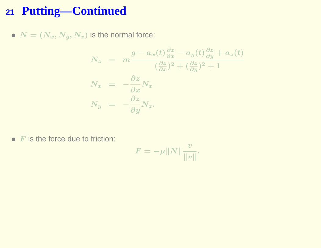
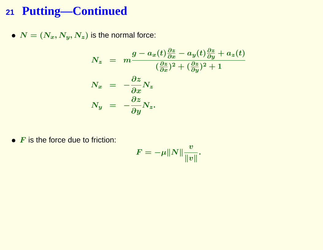
21 Putting—Continued
• N = (Nx, Ny, Nz) is the normal force:
Nz = mg − ax(t)∂z
∂x− ay(t)∂z
∂y+ az(t)
(∂z∂x
)2 + (∂z∂y
)2 + 1
Nx = −∂z
∂xNz
Ny = −∂z
∂yNz.
• F is the force due to friction:
F = −µ‖N‖v
‖v‖.

21 Putting—Continued
• N = (Nx, Ny, Nz) is the normal force:
Nz = mg − ax(t)∂z
∂x− ay(t)∂z
∂y+ az(t)
(∂z∂x
)2 + (∂z∂y
)2 + 1
Nx = −∂z
∂xNz
Ny = −∂z
∂yNz.
• F is the force due to friction:
F = −µ‖N‖v
‖v‖.
21 Putting—Continued
• N = (Nx, Ny, Nz) is the normal force:
Nz = mg − ax(t)∂z
∂x− ay(t)∂z
∂y+ az(t)
(∂z∂x
)2 + (∂z∂y
)2 + 1
Nx = −∂z
∂xNz
Ny = −∂z
∂yNz.
• F is the force due to friction:
F = −µ‖N‖v
‖v‖.
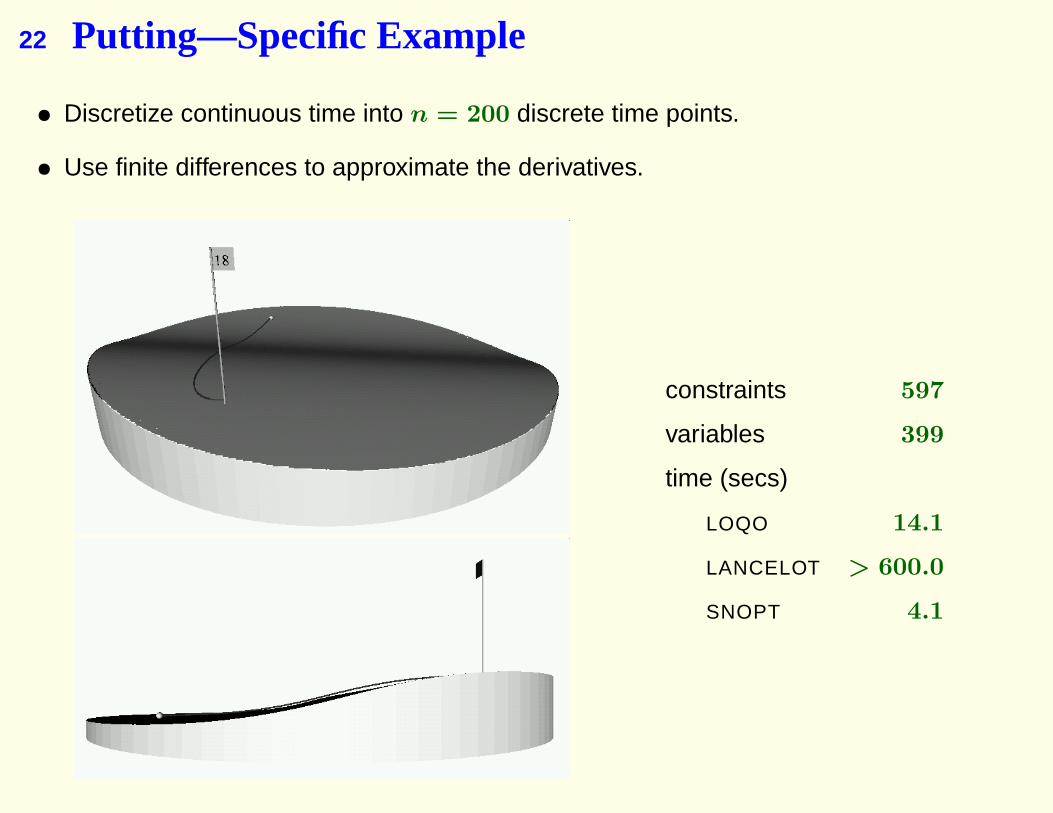
22 Putting—Specific Example
• Discretize continuous time into n = 200 discrete time points.
• Use finite differences to approximate the derivatives.
constraints 597
variables 399
time (secs)
LOQO 14.1
LANCELOT > 600.0
SNOPT 4.1

23 Goddard Rocket Problem
Objective:
maximize h(T );
Constraints:
v = h
a = v
θ = −cm
ma = (θ − σv2e−h/h0) − gm
0 ≤ θ ≤ θmax
m ≥ mmin
h(0) = 0 v(0) = 0 m(0) = 3
where
• θ = Thrust , m = mass
• θmax, g, σ, c, and h0 are given constants
• h, v, a, Th, and m are functions of time 0 ≤ t ≤ T .

23 Goddard Rocket Problem
Objective:
maximize h(T );
Constraints:
v = h
a = v
θ = −cm
ma = (θ − σv2e−h/h0) − gm
0 ≤ θ ≤ θmax
m ≥ mmin
h(0) = 0 v(0) = 0 m(0) = 3
where
• θ = Thrust , m = mass
• θmax, g, σ, c, and h0 are given constants
• h, v, a, Th, and m are functions of time 0 ≤ t ≤ T .
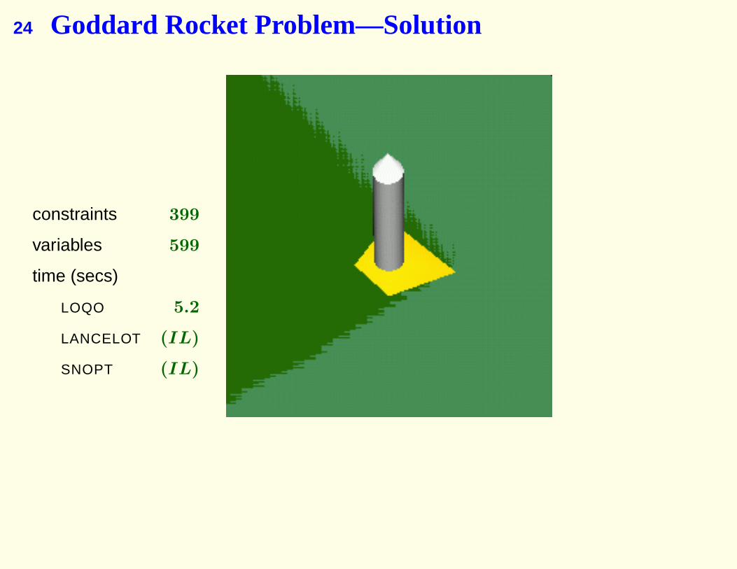
24 Goddard Rocket Problem—Solution
constraints 399
variables 599
time (secs)
LOQO 5.2
LANCELOT (IL)
SNOPT (IL)


