Interior-point methods for optimization - Cornell … · Interior-point methods for optimization...

Acta Numerica (2009), pp. 001– c© Cambridge University Press, 2009

DOI: 10.1017/S0962492904 Printed in the United Kingdom

Interior-point methods for optimization

Arkadi S. NemirovskiSchool of Industrial and Systems Engineering,

Georgia Institute of Technology,Atlanta, Georgia 30332, USA

E-mail: [email protected]

Michael J. ToddSchool of Operations Research and Information Engineering,

Cornell University, Ithaca, NY 14853, USA.E-mail: [email protected]

This article describes the current state of the art of interior-point methods(IPMs) for convex, conic, and general nonlinear optimization. We discuss thetheory, outline the algorithms, and comment on the applicability of this classof methods, which have revolutionized the field over the last twenty years.

CONTENTS

1 Introduction 12 The self-concordance-based approach to IPMs 43 Conic optimization 194 IPMs for nonconvex programming 365 Summary 38References 39

1. Introduction

During the last twenty years, there has been a revolution in the methodsused to solve optimization problems. In the early 1980s, sequential quadraticprogramming and augmented Lagrangian methods were favored for nonlin-ear problems, while the simplex method was basically unchallenged for linearprogramming. Since then, modern interior-point methods (IPMs) have in-fused virtually every area of continuous optimization, and have forced greatimprovements in the earlier methods. The aim of this article is to describeinterior-point methods and their application to convex programming, special

2 A. S. Nemirovski and M. J. Todd

conic programming problems (including linear and semidefinite program-ming), and general possibly nonconvex programming. We have also tried tocomplement the earlier articles in this journal by Wright (1992), Lewis andOverton (1996), and Todd (2001).

Almost twenty-five years ago, Karmarkar (1984) proposed his projectivemethod to solve linear programming problems: from a theoretical point ofview, this was a polynomial-time algorithm, in contrast to Dantzig’s sim-plex method. Moreover, with some refinements it proved a very worthycompetitor in practical computation, and substantial improvements to bothinterior-point and simplex methods have led to the routine solution of prob-lems (with hundreds of thousands of constraints and variables) that wereconsidered untouchable previously. Most commercial software, for exam-ple CPlex (Bixby 2002) and Xpress-MP (Gueret, Prins and Sevaux 2002),includes interior-point as well as simplex options.

The majority of the early papers following Karmarkar’s dealt exclusivelywith linear programming and its near relatives, convex quadratic program-ming and the (monotone) linear complementarity problem. Gill, Murray,Saunders, Tomlin and Wright (1986) showed the strong connection to ear-lier barrier methods in nonlinear programming; Renegar (1988) and Gonzaga(1989) introduced path-following methods with an improved iteration com-plexity; and Megiddo (1989) suggested, and Monteiro and Adler (1989) andKojima, Mizuno and Yoshise (1989) realized, primal-dual versions of thesealgorithms, which are the most successful in practice.

At the same time, Nesterov and Nemirovski were investigating the newmethods from a more fundamental viewpoint: what are the basic proper-ties that lead to polynomial-time complexity? It turned out that the keyproperty is that the barrier function should be self-concordant. This seemedto provide a clear, complexity-based criterion to delineate the class of opti-mization problems that could be solved in a provably efficient way using thenew methods. The culmination of this work was the book (Nesterov andNemirovski 1994), whose complexity emphasis contrasted with the classictext on barrier methods by Fiacco and McCormick (1968).

Fiacco and McCormick describe the history of (exterior) penalty and bar-rier (sometimes called interior penalty) methods; other useful references are(Nash 1998, Forsgren, Gill and Wright 2002). Very briefly, Courant (1943)first proposed penalty methods, while Frisch (1955) suggested the logarith-mic barrier method and Carroll (1961) the inverse barrier method (whichinspired Fiacco and McCormick). While these methods were among themost successful for solving constrained nonlinear optimization problems inthe 1960s, they lost favor in the late 1960s and 1970s when it became ap-parent that the subproblems that needed to be solved became increasinglyill-conditioned as the solution was approached.

The new research alleviated these fears to some extent, at least for certain

Interior-point methods for optimization 3

problems. In addition, the ill-conditioning turned out to be relatively be-nign — see, e.g., (Wright 1992, Forsgren, Gill and Wright 2002). Moreover,Nesterov and Nemirovski (1994) showed that, at least in principle, any con-vex optimization problem could be provided with a self-concordant barrier.This was purely an existence result, however, as the generated barrier couldnot be efficiently evaluated in general. (So we should qualify our earlierstatement: the class of optimization problems to which the new methodscan be efficiently applied consists of those with a computationally tractableself-concordant barrier.) To contrast with the general case, Nesterov andNemirovski listed a considerable number of important problems where com-putationally tractable self-concordant barriers were available, and provideda calculus for constructing such functions for more complicated sets. A verysignificant special case was that of the positive semidefinite cone, leadingto semidefinite programming. Independently, Alizadeh (1995) developed anefficient interior-point method for semidefinite programming, with the moti-vation of obtaining strong bounds for combinatorial optimization problems.

The theory of self-concordant barriers is limited to convex optimization.However, this limitation has become less burdensome as more and more sci-entific and engineering problems have been shown to be amenable to convexoptimization formulations. Researchers in control theory have been muchinfluenced by the ability to solve semidefinite programming problems (orlinear matrix inequalities, in their terminology) arising in their field — seeBoyd, El Ghaoui, Feron and Balakrishnan (1994). Moreover, a number ofseemingly nonconvex problems arising in engineering design can be reformu-lated as convex optimization problems: see Boyd and Vandenberghe (2004)and Ben-Tal and Nemirovski (2001).

Besides the books we have cited, other useful references include the lecturenotes of Nemirovski (2004) and the books of Nesterov (2003) and Renegar(2001) for general convex programming; for mostly linear programming, thebooks of Roos, Terlaky and Vial (1997), Vanderbei (2007), Wright (1997),and Ye (1997); for semidefinite programming, the handbook of Wolkowicz,Saigal and Vandenberghe (2000); and for general nonlinear programming,the survey articles of Forsgren, Gill and Wright (2002) and Gould, Orbanand Toint (2005).

In Section 2, we discuss self-concordant barriers and their properties, andthen describe interior-point methods for both general convex optimizationproblems and conic problems, as well as the calculus of self-concordant barri-ers. Section 3 treats conic optimization in detail, concentrating on symmet-ric or self-scaled cones, including the nonnegative orthant (linear program-ming) and the positive semidefinite cone (semidefinite programming). Wealso briefly discuss some recent developments in hyperbolicity cones, globalpolynomial optimization, and copositive programming. Finally, Section 4is concerned with the application of interior-point methods to general, pos-


sibly nonconvex, nonlinear optimization. These methods are used in someof the most effective codes for such problems, such as IPOPT (Wachterand Biegler 2006), KNITRO (Byrd, Nocedal and Waltz 2006), and LOQO(Vanderbei and Shanno 1999).

We have concentrated on the theory and application in structured convexprogramming of interior-point methods, since the polynomial-time complex-ity of these methods and its range of applicability have been a major focus ofthe research of the last twenty years. For further coverage of interior-pointmethods for general nonlinear programming we recommend the survey ar-ticles of Forsgren, Gill and Wright (2002) and Gould et al. (2005). Also, toconvey the main ideas of the methods, we have given short shrift to impor-tant topics including attaining feasibility from infeasible initial points, deal-ing with infeasible problems, and superlinear convergence. The literature oninterior-point methods is huge, and the area is still very active; the readerwishing to follow the latest research is advised to visit the OptimizationOnline website http://www.optimization-online.org/ and the Interior-Point Methods Online page at http://www-unix.mcs.anl.gov/otc/InteriorPoint/.A very useful source is Helmberg’s semidefinite programming pagehttp://www-user.tu-chemnitz.de/ helmberg/semidef.html. Softwarefor optimization problems, including special-purpose algorithms for semidefi-nite and second-order cone programming, is available atthe Network Enabled Optimization System (NEOS) homepagehttp://neos.mcs.anl.gov/neos/solvers/index.html.

2. The self-concordance-based approach to IPMs

Preliminaries. The first path-following interior-point polynomial-time meth-ods for linear programming, analysed by Renegar (1988) and Gonzaga (1989),turned out to belong to the very well-known interior penalty scheme goingback to Fiacco and McCormick (1968). Consider a convex program

mincT x : x ∈ X, (2.1)

X being a closed convex domain (i.e., a closed convex set with a nonemptyinterior) in Rn; this is one of the universal forms of a convex program.In order to solve the problem with a path-following scheme, one equipsX with an interior penalty or barrier F — a smooth and strongly convex(Hessian positive definite everywhere) function defined on int X such thatF (xk) → +∞ along every sequence of points xk ∈ intX converging to apoint x ∈ ∂X, and considers the barrier family of functions

Ft(x) = tcT x + F (x) (2.2)

where t > 0 is the penalty parameter. Under mild assumptions (e.g., whenX is bounded), every function Ft attains its minimum on intX at a unique


point x∗(t), and the central path x∗(t) : t ≥ 0 converges, as t → ∞,to the optimal set of (2.1). The path-following scheme for solving (2.1)suggests “tracing” this path as t →∞ according to the following conceptualalgorithm:

Given the current iterate (tk > 0, xk ∈ intX) with xk “reasonably close” to x∗(tk),wea) replace the current value tk of the penalty parameter with a larger value tk+1;andb) run an algorithm for minimizing Ftk+1(·), starting at xk, until a point xk+1 closeto x∗(tk+1) = argmin int X Ftk+1(·) is found.As a result, we get a new iterate (tk+1, xk+1) “close to the path” and loop to stepk + 1.

The main advantage of the scheme described above is that x∗(t) is, es-sentially, the unconstrained minimizer of Ft, which allows the use in b) ofbasically any method for smooth convex unconstrained minimization, e.g.,the Newton method. Note, however, that the classical theory of the path-following scheme did not suggest its polynomiality; rather, the standard the-ory of unconstrained minimization predicted slow-down of the process as thepenalty parameter grows. In sharp contrast to this common wisdom, bothRenegar and Gonzaga proved that, when applied to the logarithmic barrierF (x) = −

∑i ln(bi − aT

i x) for a polyhedral set X = x : aTi x ≤ bi, 1 ≤ i ≤

m, a Newton-method-based implementation of the path-following schemecan be made polynomial. These breakthrough results were obtained via anad hoc analysis of the behaviour of the Newton method as applied to thelogarithmic barrier (augmented by a linear term). In a short time Nesterovrealized what intrinsic properties of the standard log-barrier are responsi-ble for this polynomiality, and this crucial understanding led to the generalself-concordance-based theory of polynomial-time interior-point methods de-veloped in Nesterov and Nemirovski (1994); this theory explained the natureof existing interior-point methods (IPMs) for LP and allowed the extensionof these methods to the entire field of convex programming. We now providean overview of the basic results of this theory1.

2.1. Self-concordance

In retrospect, the notion of self-concordance can be extracted from analy-sis of the classical results on the local quadratic convergence of Newton’smethod as applied to a smooth convex function f with nonsingular Hessian.These results state that a quantitative description of the domain of quadratic

1 Up to minor refinements which can be found in (Nemirovski 2004), all results quoted inthe next subsection without explicit references are taken from (Nesterov and Nemirovski1994).


convergence depends on (a) the condition number of ∇2f evaluated at theminimizer x∗, and (b) the Lipschitz constant of ∇2f . In hindsight, sucha description seems unnatural, since it is “frame-dependent” — it heav-ily depends on an ad hoc choice of the Euclidean structure in Rn; indeed,both the condition number of ∇2f(x∗) and the Lipschitz constant of ∇2f(·)depend on this structure, which is in sharp contrast with the affine invari-ance of the Newton method itself. At the same time, a smooth stronglyconvex function f by itself defines at every point x a Euclidean structure〈u, v〉f,x = D2f(x)[u, v]. With respect to this structure, ∇2f(x) is as well-conditioned as it could be — it is just the unit matrix. The idea of Nesterovwas to use this local Euclidean structure, intrinsically linked to the functionf we intend to minimize, in order to quantify the Lipschitz constant of ∇2f ,with the ultimate goal of getting a “frame-independent” description of thebehaviour of the Newton method. The resulting notion of self-concordanceis defined as follows:

Definition 2.1. Let X ⊂ Rn be a closed convex domain. A functionf : int X → R is called self-concordant (SC) on X if

(i) f is a three times continuously differentiable convex function withf(xk) →∞ if xk → x ∈ ∂X; and

(ii) f satisfies the differential inequality

|D3f(x)[h, h, h]| ≤ 2(D2f(x)[h, h]

)3/2 ∀(x ∈ intX, h ∈ Rn). (2.3)

Given a real ϑ ≥ 1, F is called a ϑ-self-concordant barrier (ϑ-SCB) for X ifF is self-concordant on X and, in addition,

|DF (x)[h]| ≤ ϑ1/2(D2F (x)[h, h]

)1/2 ∀(x ∈ intX, h ∈ Rn). (2.4)

(As above, we will use f for a general SC function and F for a SCB in whatfollows.) Note that the powers 3/2 and 1/2 in (2.3), (2.4) are a must, since bothsides of the inequalities should be of the same homogeneity degree with respect toh. In contrast to this, the two sides of (2.3) are of different homogeneity degreeswith respect to f , meaning that if f satisfies a relation of the type (2.3) with someconstant factor on the right hand side, we always can make this factor equal to 2by scaling f appropriately. The advantage of the specific factor 2 is that with thisdefinition, the function x 7→ − ln(x) : R++ → R becomes a 1-SCB for R+ directly,without any scaling, and this function is the main building block of the theorywe are presenting. Finally, we remark that (2.3), (2.4) have a very transparentinterpretation: they mean that D2f and F are Lipschitz continuous, with constants2 and ϑ1/2, in the local Euclidean (semi)norm ‖h‖f,x =

√〈h, h〉f,x =

√hT∇2f(x)h

defined by f or similarly by F .In turns out that self-concordant functions possess nice local properties

and are perfectly well suited for Newton minimization. We are about to


present the most important of the related results. In what follows, f is aSC function on a closed convex domain X.

00: Bounds on third derivatives and the recession space of a SC function.For all x ∈ intX and all h1, h2, h3 ∈ Rn one has

|D3f(x)[h1, h2, h3]| ≤ 2‖h1‖f,x‖h2‖f,x‖h3‖f,x.

The recession subspace Ef = h : D2f(x)[h, h] = 0 of f is independent ofx ∈ intX, and X = X + Ef . In particular, if ∇2f(x) is positive definite atsome point in intX, then ∇2f(x) is positive definite for all x ∈ intX (inthis case, f is called a nondegenerate SC function; this is always the casewhen X does not contain lines).

It is convenient to write A 0 (A 0) to denote that the symmetricmatrix A is positive definite (semidefinite), and A B and B A (A Band B ≺ A) if A−B 0 (A−B 0).

10. Dikin’s ellipsoid and the local behaviour of f . For every x ∈ intX, theunit Dikin ellipsoid of f y : ‖y − x‖f,x ≤ 1 is contained in X, and withinthis ellipsoid, f is nicely approximated by its second-order Taylor expansion:

r := ‖h‖f,x < 1 ⇒(1− r)2∇2f(x) ∇2f(x + h) 1

(1−r)2∇2f(x),

f(x) +∇f(x)T h + ρ(−r) ≤ f(x + h) ≤ f(x) +∇f(x)T h + ρ(r).(2.5)

where ρ(s) := − ln(1− s)− s = s2/2 + s3/3 + . . . . (Indeed, the lower boundin the last line holds true for all h such that x + h ∈ intX.)

20. The Newton decrement and the damped Newton method. Let f be non-degenerate. Then ‖ · ‖f,x is a norm, and its conjugate norm is ‖η‖∗f,x =max

hT η : ‖h‖f,x ≤ 1

=√

ηT [∇2f(x)]−1η. The quantity

λ(x, f) := ‖∇f(x)‖∗f,x = ‖[∇2f(x)]−1∇f(x)‖f,x

= maxhDf(x)[h] : D2f(x)[h, h] ≤ 1,

called the Newton decrement of f at x, is a finite continuous function ofx ∈ intX which vanishes exactly at the (unique, if any) minimizer xf off on intX; this function can be considered as the “observable” measureof proximity of x to xf . The Newton decrement possesses the followingproperties:

λ(x, f) < 1 ⇒

argmin int X f 6= ∅ (a)f(x)−minint X f ≤ ρ(λ(x, f)) (b)‖xf − x‖f,x ≤ λ(x,f)

1−λ(x,f) (c)

‖xf − x‖f,xf≤ λ(x,f)

1−λ(x,f) . (d)

(2.6)


In particular, when it is at most 1/2, the Newton decrement is, withinan absolute constant factor, the same as ‖x − xf‖f,x, ‖x − xf‖f,xf

, and√f(x)−minint X f .The Damped Newton method as applied to f is the iterative process

xk+1 = xk −1

1 + λ(xk, f)[∇2f(xk)]−1∇f(xk) (2.7)

starting at a point x0 ∈ intX. The damped Newton method is well defined:all its iterates belong to intX. Besides this, setting λj := λ(xj , f), we have

λk+1 ≤ 2λ2k and f(xk)− f(xk+1) ≥ ρ(−λk) = λk − ln(1 + λk). (2.8)

As a consequence of (2.8), (2.7), we get the following “frame- and data-inde-pendent” description of the convergence properties of the damped Newtonmethod as applied to a SC function f : the domain of quadratic convergenceis x : λ(x, f) ≤ 1/4; after this domain is reached, every step of the methodnearly squares the Newton decrement, the ‖·‖f,xf

-distance to the minimizerand the residual in terms of f . Before the domain is reached, every stepof the method decreases the objective by at least Ω(1) = 1/4 − ln(5/4).It follows that a nondegenerate SC function admits its minimum on theinterior of its domain if and only if it is bounded below, and if and only ifλ(x, f) < 1 for certain x. Whenever this is the case, for every ε ∈ (0, 0.1]the number of steps N of the damped Newton method which ensures thatf(xk) ≤ minint X f +ε does not exceed O(1) [ln ln(1/ε) + f(x0)−minint X f ].(Here and below, O(1) denotes a suitably chosen absolute constant.)

30. Self-concordance and Legendre transformations. Let f be nondegener-ate. Then the domain y : f∗(y) < ∞ of the (modified) Legendre transfor-mation

f∗(y) = supx∈int X

[−yT x− f(x)

]of f is an open convex set, f∗ is self-concordant on the closure X∗ of this set,and the mappings x 7→ −∇f(x) and y 7→ −∇f∗(y) are bijections of intXand intX∗ that are inverse to each other. Besides this, X∗ is a closed conewith a nonempty interior, specifically, the cone dual to the recession cone ofX.

We next list specific properties of SCBs not shared by more general SCfunctions. In what follows, F is a nondegenerate ϑ-SCB for a closed convexdomain X.

40. Nondegeneracy, semiboundedness, attaining minimum. F is nondegen-erate if and only if X does not contain lines. One has

∀(x ∈ intX, y ∈ X) : ∇F (x)T (y − x) ≤ ϑ (2.9)


(semiboundedness) and

∀(x ∈ intX, y ∈ X with ∇F (x)T (y−x) ≥ 0) : ‖y−x‖F,x ≤ ϑ+2√

ϑ. (2.10)

F attains its minimum on intX if and only if X is bounded; otherwiseλ(x, F ) ≥ 1 for all x ∈ intX.

50. Useful bounds. For x ∈ intX, let πx(y) = inft : t > 0, x + t−1(y − x) ∈X be the Minkowski function of X with respect to x. One has

∀(x, y ∈ intX) :

F (y) ≤ F (x) + ϑ ln(

11−πx(y)

)F (y) ≥ F (x) +∇F (x)T (y − x) + ln

(1

1−πx(y)

)− πx(y).

(2.11)

60. Existence of the central path and its convergence to the optimal set.Consider problem (2.1) and assume that the domain X of the problem isequipped with a self-concordant barrier F , and the level sets of the objec-tive x ∈ X : cT x ≤ α are bounded. In the situation in question, F isnondegenerate, cT x attains its minimum on X, the central path

x∗(t) := argminx∈int X

Ft(x), Ft(x) := tcT x + F (x), t > 0,

is well-defined, all functions Ft are self-concordant on X and

ε(x∗(t)) := cT x∗(t)−minx∈X

cT x ≤ ϑ

t, t > 0. (2.12)

Moreover, if λ(x, Ft) ≤ 12 for some t > 0, then

ε(x) ≤ ϑ +√

ϑ

t. (2.13)

Let us derive the claims in 60 from the preceding facts, mainly in order to explainwhy these facts are important. By 10, F is nondegenerate, since X does not containlines. The fact that all Ft are SC is evident from the definition — self-concordanceclearly is preserved when adding a linear or convex quadratic function to an SCone. Further, the level sets of the objective on X are bounded, so that the objectiveattains its minimum over X at some point x∗ and, as is easily seen, is coercive onX: cT x ≥ α + β‖x‖ for all x ∈ X with appropriate constants β > 0 and α. (‖ · ‖,without subscripts, always denotes the Euclidean norm.) Now fix a point y in intX;then πx(y) ≤ ‖y−x‖

r+‖y−x‖ for all x ∈ intX, where r > 0 is such that a ‖ · ‖-ball ofradius r centered at y belongs to X. Invoking the first line of (2.11) with y = y,we conclude that F (x) ≥ F (y)+ϑ ln( r

r+‖x−y‖ ) for all x ∈ intX. Recalling that theobjective is coercive, we conclude that Ft(x) →∞ as x ∈ X and ‖x‖ → ∞, so thatthe level sets of Ft are bounded. Since Ft is, along with F , an interior penalty for X,these sets are in fact compact subsets of intX, whence Ft attains its minimum onintX. Since Ft is convex and nondegenerate along with F , the minimizer is unique;


thus, the central path is well-defined. To verify (2.12), note that ∇F (x∗(t)) = −tc,whence cT (x∗(t) − y) = t−1∇F (x∗(t)T (y − x∗(t)). By (2.9), the right hand sidein this equality is at most ϑ/t, provided y ∈ X, and (2.12) follows. Finally, whenλ(x, Ft) ≤ 1/2, then ‖x − x∗(t)‖Ft,x∗(t) ≤ 1 by (2.6.d) as applied to Ft instead ofF . Since ‖ · ‖Ft,u ≡ ‖ · ‖F,u, we get ‖x− x∗(t)‖F,x∗(t) ≤ 1, whence cT (x− x∗(t)) ≤‖c‖∗F,x∗(t)

‖x − x∗(t)‖F,x∗(t) ≤ ‖c‖∗F,x∗(t)= t−1‖∇F (x∗(t))‖∗F,x∗(t)

≤ t−1√

ϑ, whichcombines with (2.12) to imply (2.13).

2.2. A primal polynomial-time path-following method

As an immediate consequence of the above results, we arrive at the followingimportant result:

Theorem 2.1. Consider problem (2.1) and assume that the level sets ofthe objective are bounded, and we are given a ϑ-SCB F for X; according to60, c and F define a central path x∗(·). Suppose we also have at our disposala starting pair (t0 > 0, x0 ∈ intX) which is close to the path in the sensethat λ(x0, Ft0) ≤ 0.1, and consider the following implementation (the basicpath-following algorithm) of the path-following scheme:

(tk, xk) 7→

tk+1 = (1 + 0.1ϑ−1/2)tkxk+1 = xk − 1

1+λ(xk,Ftk+1) [∇

2F (xk)]−1∇Ftk+1(xk).

(2.14)

This recurrence is well-defined (i.e., xk ∈ intX for all k), maintains closenessto the path (i.e., λ(xk, Ftk) ≤ 0.1 for all k) and ensures the efficiency estimate

∀k : cT xk −minx∈X

cT x ≤ ϑ +√

ϑ

tk≤ ϑ +

√ϑ

t0exp−0.095√

ϑk. (2.15)

In particular, for every ε > 0, it takes at most

N(ε) = O(1)√

ϑ ln(

ϑ

t0ε+ 2)

steps of the recurrence to get a strictly feasible (i.e., in intX) solution tothe problem with residual in terms of the objective at most ε.

Proof. In view of 20 and 60, all we need to prove by induction on k is that(2.14) maintains closeness to the path. Assume that (t = tk, x = xk) is closeto the path, and let us verify that the same is true for (t+ = tk+1, x+ =xk+1). Taking into account that ‖ · ‖Ft,u = ‖ · ‖F,u and similarly for theconjugate norms, we have 0.1 ≥ λ(x, Ft) = ‖tc +∇F (x)‖∗F,x so that

t‖c‖∗F,x ≤ 0.1 + ‖∇F (x)‖∗F,x

≤ 0.1 + ϑ1/2


using the fact that F is a ϑ-SCB. This implies that

λ(x, Ft+) = ‖[tc +∇F (x)] + (t+ − t)c‖∗F,x

≤ ‖tc +∇F (x)‖∗F,x + (t+/t− 1)t‖c‖∗F,x

≤ 0.1 + 0.1ϑ−1/2t‖c‖∗F,x ≤ 0.1[1 + ϑ−1/2[0.1 + ϑ1/2]] ≤ 0.21.

Finally, we obtain

λ(x+, Ft+) ≤ 2λ2(x, Ft+) ≤ 0.1,

using (2.8).

Remarks. A. The algorithm presented in Theorem 2.1 is, in a sense, incom-plete — it does not explain how to approach the central path in order tostart path-tracing. There are many ways to resolve this issue. Assume, e.g.,that X is bounded and we know in advance a point y ∈ intX. When X isbounded, every linear form gT x generates a central path, and we can easilyfind such a path passing through y — with g = −∇F (y), the correspondingpath passes through y when t = 1. Now, as t → +0, all paths converge tothe minimizer xF of F over X, and thus approach each other. At the sametime, we can as easily trace the paths backward as trace them forward —with the parameter updating rule tk+1 = (1− 0.1ϑ−1/2)tk, the recurrence inTheorem 2.1 still maintains closeness to the path, now along a sequence ofvalues of the parameter t decreasing geometrically. Thus, we can trace theauxiliary path passing through y backward until coming close to the path ofinterest, and then start tracing the latter path forward. A simple analysisdemonstrates that with simple on-line termination and switching rules, theresulting algorithm, for every ε > 0, produces a strictly feasible ε-solutionto the problem at the price of no more than O(1)

√ϑ ln

(ϑV

(1−πxF(y))ε + 2

)Newton steps of both phases, where V = maxx∈X cT x−minx∈X cT x.

B. The outlined path-following algorithm, using properly chosen SC bar-riers, yields the currently best polynomial-time complexity bounds for ba-sically all “well-structured” generic convex programs, like those of linear,second-order cone, semidefinite, and geometric programming, to name justa few. At the same time, from a practical perspective a severe shortcomingof the algorithm is its worst-case-oriented nature — as presented, it willalways perform according to its worst-case theoretical complexity bounds.There exist implementations of IPMs that are much more powerful in prac-tice using more aggressive parameter updating policies that are adjustedduring the course of the algorithm. All known algorithms of this type areprimal-dual — they work simultaneously on the problem and its dual, andnearly all of them, including all those implemented so far in professional soft-ware, work with conic problems, specifically, those of linear, second-ordercone, and semidefinite programming (the only exceptions are the cone-free


primal-dual methods proposed in (Nemirovski and Tuncel 2005); these meth-ods, however, have not yet been implemented). Our next goal is to describethe general theory of primal-dual interior-point methods for conic problems.

2.3. Interior-point methods for conic problems

Interior-point methods for conic problems are associated with specific ϑ-SCbarriers for cones — those satisfying the so-called logarithmic homogeneitycondition.

Definition 2.2. Let K ⊂ Rn be a cone (from now on, all cones areclosed and convex, have nonempty interiors, and contain no lines). A ϑ-self-concordant barrier F for K is called logarithmically homogeneous (aLHSCB), if

∀(τ > 0, x ∈ intK) : F (τx) = F (x)− ϑ ln τ. (2.16)

In fact, every self-concordant function on a cone K satisfying the identity(2.16) is automatically a ϑ-SCB for K, since whenever a smooth function Fsatisfies the identity (2.16), one has

∀(x ∈ intK) : ∇F (x)T x = −ϑ, ∇2F (x)x = −∇F (x); (2.17)

it follows that when F is self-concordant, one has

λ(x, F ) =√∇F (x)T [∇2F (x)]−1∇F (x) =

√−∇F (x)T x =

√ϑ,

meaning that F indeed is a ϑ-SCB for K. A nice and important fact is thatthe (modified) Legendre transformation F∗(s) of a ϑ-LHSCB F for a coneK is a ϑ-LHSCB for the cone

K∗ := s ∈ Rn : sT x ≥ 0,∀(x ∈ K) (2.18)

dual to K. The resulting symmetry of LHSCBs complements the symmetrybetween cones and their duals. Moreover,

Proposition 2.1. The mappings x 7→ −∇F (x) and s 7→ −∇F∗(s) areinverse bijections between intK and intK∗, and these bijections are ho-mogeneous of degree -1: −∇F (τx) = −τ−1∇F (x), x ∈ intK, τ > 0, andsimilarly for F∗. Finally, ∇2F and ∇2F∗ are homogeneous of degree -2, with∇2F∗(−∇F (x)) = [∇2F (x)]−1 and ∇2F (−∇F∗(s)) = [∇2F∗(s)]−1.utNow assume that we want to solve a primal-dual pair of conic problems

minx

cT x : Ax = b, x ∈ K

(P )

maxy,s

bT y : AT y + s = c, s ∈ K∗

(D)

(2.19)

where the rows of A are linearly independent and both problems have strictlyfeasible solutions (i.e., feasible solutions with x ∈ intK and s ∈ intK∗).


Assume also that we have at our disposal a ϑ-LHSCB F for K along withits Legendre transformation F∗, which is a ϑ-LHSCB for K∗. (P ) can betreated as a problem of the form (2.1), with the affine set L = x : Ax = bplaying the role of the “universe” Rn and K∩L in the role of X. It is easilyseen that the restriction of F to intK∩L is a ϑ-SCB for the resulting problem(2.1) (see rule D in Subsection 2.4), and that this is a problem with boundedlevel sets. As a result, we can define the primal central path x∗(t) whichis comprised of strictly feasible solutions to (P ) and converges, as t → ∞,to the primal optimal set. Similarly, setting Y = y : c − AT y ∈ K∗, thedual problem can be written in the form of (2.1), namely, as miny∈Y [−b]T y.The domain Y of this problem also can be equipped with a ϑ-SCB, namely,F∗(c − AT y), and again the problem has bounded level sets, so that wecan define the associated central path y∗(t). This induces the dual centralpath s∗(t) := c−AT y∗(t); the latter path is comprised of interior points ofK∗. We have arrived at the primal-dual central path z∗(t) := (x∗(t), s∗(t))“living” in the interior of K×K∗. It is easily seen that for every t > 0, thepoint z∗(t) is uniquely defined by the following restrictions on its componentsx, s:

x ∈ Xo := intK ∩ x : Ax = b [strict primal feasibility],s ∈ So := intK∗ ∩ s : ∃y s.t. AT y + s = c [strict dual feasibility],

s = −t−1∇F (x)x = −t−1∇F∗(s)

[augmented complementary slackness].

(2.20)Note that each of the complementary slackness equations implies, by Propo-sition 2.1, the other, so that we could eliminate either one of them; we keepboth to highlight the primal-dual symmetry.

Primal-dual path-following interior-point methods trace simultaneouslythe primal and dual central paths basically in the same fashion as the methoddescribed in Theorem 2.1. It turns out that tracing the paths together ismuch more advantageous than tracing only one of them. In our generalsetting these advantages permit, e.g.,• adaptive long-step strategies for path-tracing (Nesterov 1997);• an elegant way (“self-dual embedding”, see, e.g., (Ye, Todd and Mizuno

1994, Xu, Hung and Ye 1996, Andersen and Ye 1999, Luo, Sturm and Zhang2000, de Klerk, Roos and Terlaky 1997, Potra and Sheng 1998)) to initializepath-tracing even in the case when no strictly feasible solutions to (P) and(D) are available in advance; and• building certificates of strict (i.e., preserved by small perturbations of

the data) primal or dual infeasibility (Nesterov, Todd and Ye 1999) when itholds, etc.Primal-dual IPMs achieve their full power when the underlying cones areself-scaled, which is the case in linear, second-order cone, and semidefinite


programming, considered in depth in Section 3. In the remaining part ofthis subsection, we overview, still in the general setting, another family ofprimal-dual IPMs — those based on potential reduction.

Potential-reduction interior-point methodsWe now present two potential-reduction IPMs which are straightforwardconic generalizations, developed in (Nesterov and Nemirovski 1994), of al-gorithms originally proposed for LP.

Karmarkar’s Algorithm. The very first polynomial-time interior-point methodfor LP was discovered by Karmarkar (1984). The conic generalization ofthe algorithm is as follows. Assume that we want to solve a strictly fea-sible problem (P ) in the following special setting: the primal feasible setX := x ∈ K : Ax = b is bounded, the optimal value is known to be 0, andwe know a strictly feasible primal starting point x (using conic duality, everystrictly primal-dual feasible conic problem can be transformed to this form).Last, K is equipped with a ϑ-LHSCB F . It is immediately seen that underour assumptions b 6= 0, so that we lose nothing when assuming that the firstequality constraint reads eT x = 1 for some vector e. Subtracting this equal-ity with appropriate coefficients from the remaining equality constraints in(P ), we can make all these constraints homogeneous, thus representing theproblem in the form

minx

cT x : x ∈ L ∩K, eT x = 1

,

where L is a linear subspace in Rn. Note that since X is bounded, we haveeT x > 0 for every 0 6= x ∈ (L ∩K). If we exclude the trivial case cT x = 0(here already x is an optimal solution), cT x is positive on the relative interiorXo := X ∩ intK of X, so that the projective transformation x 7→ p(x) :=x/cT x is well defined on Xo; this transformation maps Xo onto the relativeinterior Zo := Z ∩ intK of the set Z := z : z ∈ L∩K, cT z = 1, the inversetransformation being z 7→ z/eT z. The point is that Z is unbounded, sinceotherwise the linear form eT z would be bounded and positive on Z due toeT x > 0 for 0 6= x ∈ L ∩K, and so cT x would be bounded away from 0 onXo, which is not the case. All we need is to generate a sequence zk ∈ Zo

such that ‖zk‖ → ∞ as k → ∞; indeed, for such a sequence we clearlyhave eT zk → ∞ and cT zk = 1, whence the points xk = zk/eT zk, which arefeasible solutions to the problem of interest, satisfy cT xk → 0 = minx∈X cT xas k →∞. This is how we “run to∞ along Z” using Karmarkar’s algorithm:Let G(z) be the restriction of F to Zo. Treating Z as a subset of its affinehull Aff(Z), so that Z is a closed convex domain in a certain Rn, we findthat G is a ϑ-SCB for Z (see rule D in Subsection 2.4). Since Z, along withK, does not contain lines, G is nondegenerate and therefore λ(z, G) ≥ 1 forall z ∈ Zo by 40 (recall that Z is unbounded); applying 20, we conclude


that the step z 7→ z+(z) of the damped Newton method as applied to G, zmaps Zo into Zo and reduces G by at least the absolute constant δ :=1 − ln(2) > 0. It follows that applying the damped Newton method to G,we push G to −∞, and therefore indeed run to ∞ along Z. To get anexplicit efficiency estimate, let us look at the Karmarkar potential functionφ : Xo → R defined by φ(x) = ϑ ln(cT x) + F (x); note that φ(x) = G(p(x))due to the ϑ-logarithmical homogeneity of F . It follows that the basicKarmarkar step x 7→ x+(x) = p−1(z+(p(x))) maps Xo into itself and reducesthe potential by at least δ. In Karmarkar’s algorithm, one iterates this step(usually augmented by a line search aimed at getting a larger reductionin the potential than the guaranteed reduction δ) starting with x0 := x,thus generating a sequence xk∞k=0 of strictly feasible solutions to (P ) suchthat φ(xk) ≤ φ(x) − kδ = F (x) + ϑ ln(cT x) − kδ. Recalling that X isbounded, so that F is bounded below on Xo by 40, we have also F (x) ≥F := minx∈Xo F (x), whence F (x)+ϑ ln(cT x)−kδ ≥ φ(xk) ≥ F +ϑ ln(cT xk).We arrive at the efficiency estimate

cT xk = cT xk −minx∈X

cT x ≤ cT x exp

(F (x)− F − kδ

ϑ

),

meaning that for every ε ∈ (0, 1), it takes at most b [F (x)− bF ]+ϑ ln(1/ε)δ c+1 steps

of the method to arrive at a strictly feasible solution xk with cT xk = cT xk−minX cT x ≤ εcT x. The advantage of the Karmarkar algorithm as comparedto that in Theorem 2.1 is that all we interested in now is driving the (online observable) potential function φ(x) to −∞ as rapidly as possible, whilestaying all the time strictly feasible; this can be done, e.g., by augmentingthe basic step with an appropriate line search which usually leads to a muchlarger reduction in φ(·) at each step than the reduction δ guaranteed by thetheory. As a result, the practical performance of Karmarkar’s algorithm istypically much better than predicted by the theoretical complexity estimateabove. On the negative side, the latter estimate is worse than that for thebasic path-following method from Theorem 2.1 — now the complexity isproportional to ϑ rather than to ϑ1/2 and ϑ ≥ 1 may well be large. Tocircumvent this difficulty, we now present a primal-dual potential-reductionalgorithm, extending to the general conic case the algorithm of Ye (1991)originally developed for LP.

Primal-dual potential-reduction algorithm. This algorithm is a “genuineprimal-dual one”; it works on a strictly feasible pair (2.19) of conic problemsand associates with this pair the generalized Tanabe-Todd-Ye (Tanabe 1988,Todd and Ye 1990) primal-dual potential function p : Xo × So → R definedby

p(x, s) := (ϑ+√

ϑ) ln(sT x)+F (x)+F∗(s) =: p0(x, s)+√

ϑ ln(sT x). (2.21)


It is easily seen that p0 is bounded below on Xo×So and the set of minimizersof p0 on Xo×So is exactly the primal-dual central path, where p0 takes thevalue p∗ = ϑ ln(ϑ)− ϑ. It follows that for (x, s) ∈ Xo × So, the duality gapsT x can be bounded in terms of p:

(x, s) ∈ Xo × So ⇒ sT x ≤ expϑ−1/2[p(x, s)− p∗]. (2.22)

(It can be readily checked — see Proposition 3.1 — that cT x−bT y = sT x ≥ 0for any feasible x and (y, s), so sT x bounds the distance from optimality ofboth the primal and dual objective function values.)

Hence all we need in order to approach primal-dual optimality is a “basicprimal-dual step” — an update (x, s) 7→ (x+, s+) : Xo × So → Xo × So

which reduces “substantially” — at least by a positive absolute constantδ — the potential p. Iterating this update (perhaps augmented by a linesearch aimed at further reduction in p) starting with a given initial point(x0, s0) ∈ Xo × So, we get a sequence of strictly feasible primal solutionsxk and dual slacks sk ∈ intK∗ (which can be immediately extended todual feasible solutions (yk, sk)), such that p(xk, sk) ≤ p(x0, s0) − kδ, whichcombines with (2.22) to yield the efficiency estimate

sTk xk ≤ expϑ−1/2[p0(x0, s0)− p∗] exp−δϑ−1/2ksT

0 x0.

Now it takes only O(1)√

ϑ steps to reduce the (upper bound on the) dualitygap by an absolute constant factor, and we end up with complexity boundscompletely similar to those in Theorem 2.1.

It remains to explain how to make a basic primal-dual step. This can be done asfollows: with a fixed positive threshold λ, given (x, s) ∈ Xo × So, we linearize thelogarithmic term in the potential in x and in s, thus getting the functions

ξ 7→ px(ξ) = (ϑ +√

ϑ) sT ξsT x

+ F (ξ) + constx : intK → R,

σ 7→ ps(σ) = (ϑ +√

ϑ)σT xsT x

+ F∗(σ) + consts : intK∗ → R,

which are nondegenerate self-concordant functions on K and K∗, respectively. Wecompute the Newton direction dx = argmin ddT∇px(x) + 1

2dT∇2px(x)d : x + d ∈Aff(X) of px

∣∣X

at ξ = x along with the corresponding Newton decrement λ :=λ(x, px

∣∣X

) =√−∇px(x)T dx. When λ ≥ λ, one can set s+ = s and take for x+ the

damped Newton iterate x + (1 + λ)−1dx of x, the Newton method being appliedto px

∣∣X

. When λ < λ, one can set x+ = x and s+ = sT xϑ+

√ϑ[−∇F (x)−∇2F (x)dx].

It can be shown that with a properly chosen absolute constant λ > 0, this updateindeed ensures that (x+, s+) ∈ Xo × So and p(x+, s+) ≤ p(x, s) − δ, where δ > 0depends solely on λ. Note that the same is true for the “symmetric” updatingobtained by similar construction with the primal and dual problems swapped, andone is welcome to use the better (the one with a larger reduction in the potential)of these two updates or their line search augmentations.


2.4. The calculus of self-concordant barriers

The practical significance of the nice results we have described dependsheavily on our ability to equip the problem we are interested in (a convexprogram (2.1), or a primal-dual pair of conic programs (2.19)) with self-concordant barrier(s). In principle this can always be done: every closedconvex domain X ⊂ Rn admits an O(1)n-SCB; when the domain is a cone,this barrier can be chosen to be logarithmically homogeneous. Assumingw.l.o.g. that X does not contain lines, one can take as such a barrier thefunction

F (x) = O(1) lnmesny : yT (z − x) ≤ 1 ∀z ∈ X

where mesn denotes n-dimensional (Jordan or Lebesgue) measure. Thisfunction has a transparent geometric interpretation: the set whose measurewe are taking is the polar of X − x. When X is a cone (closed, convex,containing no lines and with a nonempty interior), the universal barriergiven by the expression above is automatically logarithmically homogeneous.From a practical perspective, the existence theorem just formulated is of notmuch interest — the universal barrier usually is pretty difficult to compute,and in the rare cases when this is possible, it may be non-optimal in terms ofits self-concordance parameter. Fortunately, there exists a simple and fullyalgorithmic “calculus” of self-concordant barriers which allows us to buildsystematically explicit efficiently computable SCBs for seemingly all genericconvex programs associated with “computationally tractable” domains. Westart with the list of the most basic rules (essentially, the only ones neededin practice) of “self-concordant calculus”.A. If F is a ϑ-SCB for X and α ≥ 1, then αF is an (αϑ)-SCB for X;B. [direct products] Let Fi, i = 1, ...,m, be ϑi-SCBs for closed convex do-mains Xi ⊂ Rni . The “direct sum” F (x1, ..., xm) =

∑i Fi(xi) of these

barriers is a (∑

i ϑi)-SCB for the direct product X = X1 × ... ×Xm of thesets;C. [intersection] Let Fi, i = 1, ...,m, be ϑi-SCBs for closed convex domainsXi ⊂ Rn, and let the set X =

⋂i Xi possess a nonempty interior. Then

F (x) =∑

i Fi(x) is a (∑

i ϑi)-SCB for X;D. [inverse affine image] Let F be a ϑ-SCB for a closed convex domainX ⊂ Rn, and y 7→ Ay + b : Rk → Rn be an affine mapping whose imageintersects intX. Then the function G(y) = F (Ay + b) is a ϑ-SCB for theclosed convex domain Y = y : Ay + b ∈ X.

When the operands in the rules are cones and the original SCBs are log-arithmically homogeneous, so are the resulting barriers (in the case of D,provided that b = 0). All the statements remain true when, instead ofSCBs, we are speaking about SC functions; in this case, the parameter-


related parts should be skipped, and what remains become statements onpreserving self-concordance.

Essentially all we need in addition to the outlined (and nearly evident)elementary calculus rules, are two more advanced rules as follows.E. [taking the conic hull] Let X ⊂ Rn be a closed convex domain and Fbe a ϑ-SCB for X. Then, with a properly chosen absolute constant κ, thefunction F+(x, t) = κ[F (x/t)− 2ϑ ln t] is a 2κϑ-SCB for the conic hull

X+ := cl (x, t) ∈ Rn × R : t > 0, x/t ∈ intX .

of X.To present the last calculus rule, which can be skipped on a first reading,

we need to introduce the notion of compatibility as follows. Let K ⊂ RN andG− ⊆ Rn be a closed convex cone and a closed convex domain, respectively,let β ≥ 1, and let A(x) : int G− → RN be a mapping. We say that Ais β-compatible with K, if A is three times continuously differentiable onintG−, is K-concave (that is, D2A(x)[h, h] ∈ −K for all x ∈ intG− and allh ∈ Rn) and

D3A(x)[h, h, h] ≤K −3βD2A(x)[h, h]

for all x ∈ intG− and h ∈ Rn with x ± h ∈ G−, where a ≤K b means thatb− a ∈ K. The calculus rule in question reads:F. Let G− ⊂ Rn, G+ ⊂ RN be closed convex domains and A : int G− → RN

be a mapping, β-compatible with the recession cone of G+, whose imageintersects intG+. Given ϑ±-SCBs F± for G+ and G−, respectively, let usdefine F : Xo := x ∈ intG− : A(x) ∈ intG+ → R by

F (x) = F+(A(x)) + β2F−(x).

Then F is a (ϑ+ + β2ϑ−)-SCB for X = clXo.

The most nontrivial and important example of a mapping which can be used in thecontext of rule E is the fractional-quadratic substitution. Specifically, let T , E, Fbe Euclidean spaces, Q(x, z) : E × E → F be a symmetric bilinear mapping andA(t) be a symmetric linear operator on E affinely depending on t ∈ T and suchthat the bilinear form Q(A(t)x, z) on E × E is symmetric in x, z for every t ∈ T .Further, let K be a closed convex cone in F such that Q(x, x) ∈ K for all x, and Hbe a closed convex domain in T such that A(t) is positive definite for all t ∈ intH.It turns out that the mapping A(y, x, t) = y − Q([A(t)]−1x, x) with the domainF × E × intH is 1-compatible with K.

It turns out (see examples in (Nesterov and Nemirovski 1994, Nemirovski2004)) that the combination rules A - F used “from scratch” — from the soleobservation that the function − lnx is a 1-LHSCB for the nonnegative ray— permit one, nearly without calculations, to build “good” SCBs/LHSCBsfor all interesting convex domains/cones, including epigraphs of numerousconvex functions (e.g., the elementary univariate functions like powers and


the exponential, and the multivariate p-norms), sets given by finite systemsof convex linear and quadratic inequalities, and much more. This list in-cludes, in particular, ϑ-LHSCBs underlying (a) the nonnegative orthant Rn

+

(F (x) = −∑

j lnxj , ϑ = n), (b) Lorentz cones Lq = (ξ, x) ∈ R × Rq : ξ ≥‖x‖2 (F (ξ, x) = − ln(ξ2−xT x), ϑ = 2), (c) semidefinite cones Sp

+ (the coneof all symmetric positive definite matrices of order p) (F (x) = − ln det(x),ϑ = p) and (d) matrix norm cones (ξ, x) : ξ ≥ 0, x ∈ Rp×q : ξ2Iq xT x(assuming w.l.o.g. p ≥ q, F (ξ, x) = − ln det(ξIq− ξ−1xT x)− ln ξ, ϑ = q +1).

In regards to (a)-(d), (a) is self-evident, and the remaining three barriers can beobtained from (a) and F, without calculations, via the above result on fractional-quadratic substitution. E.g., to get (b), we set T = F = R, E = Rn = Rn×1,Q(x, z) = xT z, A(ξ) = ξIn, K = H = R+, thus concluding that the mappingA(y, x, ξ) = y − ξ−1xT x with the domain intG−, G− = y ∈ R × x ∈ Rn ×ξ ≥ 0, taking values in R, is 1-compatible with K = R+. Applying F withthe just defined G− and with G+ = R+, F−(y, x, ξ) = − ln ξ, F+(s) = − ln s andusing (a) and D to conclude that F− and F+ are SCBs for G− and G+ with theparameters ϑ− = ϑ+ = 1, we see that − ln(y − ξ−1xT x) − ln ξ is a 2-SCB for theset (y, x, ξ) : yξ ≥ xT x, y, ξ ≥ 0. It remains to note that Ln is the inverse affineimage of the latter set under the linear mapping (ξ, x) 7→ (ξ, x, ξ), and to apply D.

Note that (a)-(c) combine with B to induce LHSCBs for the direct productsK of nonnegative rays, Lorentz and semidefinite cones. All cones K one canget in this fashion are self-dual, and the resulting barriers F turn out to be“self-symmetric” (F∗(·) = F (·) + constK), thus giving rise to primal-dualIPMs for linear, conic quadratic, and semidefinite programming. Moreover,it turns out that the barriers in question are “optimal” — with provablyminimum possible values of the self-concordance parameter ϑ.

3. Conic optimization

Here we treat in more detail the case of the primal-dual conic problems in(2.19). We restate the primal problem:

minx cT x(P ) Ax = b,

x ∈ K,

where again c ∈ IRn, A ∈ IRm×n, b ∈ IRm, and K is a closed convex conein IRn. We call this the conic programming problem in primal or standardform, since when K is the nonnegative orthant, it becomes the standard-form linear programming problem.

Recall the dual cone defined by

K∗ := s ∈ IRn : sT x ≥ 0 for all x ∈ K. (3.1)

Then we can construct the conic programming problem in dual form using


the same data:

maxy,s bT y(D) AT y + s = c,

s ∈ K∗,

with y ∈ IRm, where we have introduced the dual slack variable s to makethe later analysis cleaner. In terms of the variables y, we have the conicconstraints c−AT y ∈ K∗, corresponding to the linear inequality constraintsc−AT y ≥ 0 when (P ) is the standard linear programming problem.

In fact, it is easy to see that (D) is the Lagrangian dual

maxy

minx∈K

cT x− (Ax− b)T y

of (P ), using the fact that minuT x : x ∈ K is 0 if u ∈ K∗ and −∞otherwise. We can also easily check weak duality:

Proposition 3.1. If x is feasible in (P ) and (y, s) in (D), then

cT x ≥ bT y,

with equality iff sT x = 0.

Proof. Indeed,

cT x− bT y = (AT y + s)T x− (Ax)T y = sT x ≥ 0, (3.2)

with the inequality following from the definition of the dual cone. utIn the case of linear programming, when K (and then also K∗) is the

nonnegative orthant, then whenever (P ) or (D) is feasible, we have equalityof their optimal values (possibly ±∞), and if both are feasible, we havestrong duality: no duality gap, and both optimal values attained.

In the case of more general conic programming, these properties no longerhold (we will provide examples in the next subsection), and we need fur-ther regularity conditions. Nesterov and Nemirovski (1994), Theorem 4.2.1,prove

Theorem 3.1. If either (P ) or (D) is bounded and has a strictly feasiblesolution (i.e., a feasible solution where x (resp., s) lies in the interior ofK (resp., K∗)), then their optimal values are equal. If both have strictlyfeasible solutions, then strong duality holds.

The existence of an easily stated dual problem provides one motivationfor considering problems in conic form (but its usefulness depends on hav-ing a closed form expression for the dual cone). We will also see that manyimportant applications naturally lead to conic optimization problems. Fi-nally, there are efficient primal-dual interior-point methods for this class ofproblems, or at least for important subclasses.


In Subsection 3.1, we consider several interesting special cases of (P ) and(D). Subsection 3.2 discusses path-following interior-point methods. InSubsection 3.3, we consider a special class of conic optimization problemsallowing symmetric primal-dual methods, and the final subsection addressesrecent extensions.

3.1. Examples of conic programming problems

First of all, it is worth pointing out that any convex programming problemcan be put into conic form. Without loss of generality, after introducing anew variable if necessary to represent a convex nonlinear objective function,we can assume that the original problem is

minxcT x : x ∈ X,

with X a closed convex subset of IRn. This is equivalent to the conic opti-mization problem in one dimension higher:

minx,ξ

cT x : ξ = 1, (x, ξ) ∈ K,

where K := cl(x, ξ) ∈ IRn × IR : ξ > 0, x/ξ ∈ X. However, this for-mal equivalence may not be very useful practically, partly because K andK∗ may not be easy to work with. More importantly, even if we have agood self-concordant barrier for X, it may be hard to obtain an efficientself-concordant barrier for K (although general, if usually overconservative,procedures are available: see rule E in Subsection 2.4 and (Freund, Jarreand Schaible 1996)).

Let us turn to examples with very concrete and useful cones. The firstexample is of course linear programming, where K = IRn

+. Then it is easy tosee that K∗ is also IRn

+, and so the dual constraints are just AT y ≤ c. Thesignificance and wide applicability of linear programming are well-known.Our first case with a non-polyhedral cone is what is known as second-ordercone programming (SOCP). Here K is a second-order, or Lorentz, or “ice-cream” cone,

Lq := (ξ, x) ∈ IR× IRq : ξ ≥ ‖x‖,

or the product of such cones. It is not hard to see, using the Cauchy-Schwarzinequality, that such cones are also self-dual, i.e., equal to their duals. Wenow provide an example showing the usefulness of SOCP problems (manymore examples can be found in (Lobo, Vandenberghe, Boyd and Lebret1998) and in (Ben-Tal and Nemirovski 2001)), and also a particular instancedemonstrating that strong duality does not always hold for such problems.

Suppose we are interested in solving a linear programming problemmaxbT y : AT y ≤ c, but the constraints are not known exactly: for the jthconstraint aT

j y ≤ cj , we just know that (cj ; aj) ∈ (cj ; aj)+Pjuj : ‖uj‖ ≤ 1,


an ellipsoidal uncertainty set centered at the nominal values (cj ; aj). (Weuse the MATLAB-like notation (u; v) to denote the concatenation of thevectors u and v.) Here Pj is a suitable matrix that determines the shapeand size of this uncertainty set. We would like to choose our decision vari-able y so that it is feasible no matter what the constraint coefficients turnout to be, as long as they are in the corresponding uncertainty sets; withthis limitation, we would like to maximize bT y. This is (a particular caseof) the so-called robust linear programming problem. Since the minimum ofcj − aT

j y = (cj ; aj)T (1;−y) over the jth uncertainty set is

(cj ; aj)T (1;−y) + min(Pjuj)T (1;−y) : ‖uj‖ ≤ 1= (cj ; aj)T (1;−y)− ‖P T

j (1;−y)‖,

this robust linear programming problem can be formulated as

max bT y−cj + aT

j y + sj1 = 0, j = 1, . . . ,m,

P Tj (1;−y) + sj = 0, j = 1, . . . ,m,

(sj1; sj) ∈ Kj , j = 1, . . . ,m,

where each Kj is a second-order cone of appropriate dimension. This is aSOCP problem in dual form.

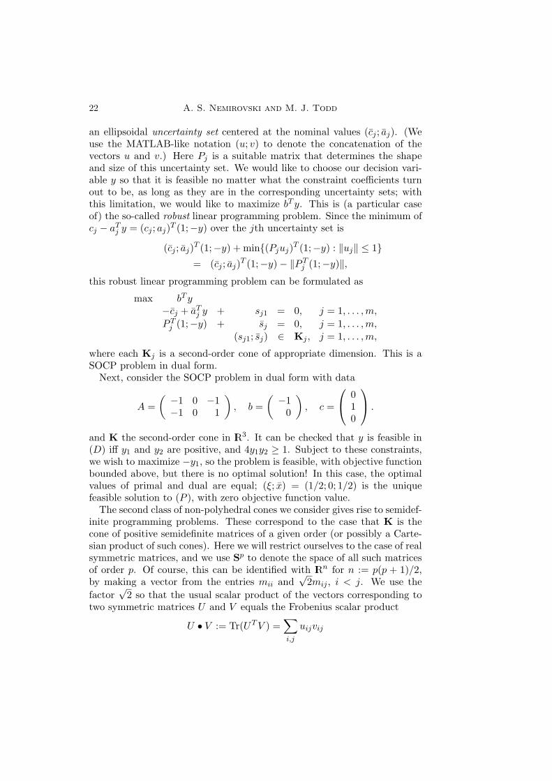
Next, consider the SOCP problem in dual form with data

A =(−1 0 −1−1 0 1

), b =

(−1

0

), c =

010

.

and K the second-order cone in IR3. It can be checked that y is feasible in(D) iff y1 and y2 are positive, and 4y1y2 ≥ 1. Subject to these constraints,we wish to maximize −y1, so the problem is feasible, with objective functionbounded above, but there is no optimal solution! In this case, the optimalvalues of primal and dual are equal; (ξ; x) = (1/2; 0; 1/2) is the uniquefeasible solution to (P ), with zero objective function value.

The second class of non-polyhedral cones we consider gives rise to semidef-inite programming problems. These correspond to the case that K is thecone of positive semidefinite matrices of a given order (or possibly a Carte-sian product of such cones). Here we will restrict ourselves to the case of realsymmetric matrices, and we use Sp to denote the space of all such matricesof order p. Of course, this can be identified with IRn for n := p(p + 1)/2,by making a vector from the entries mii and

√2mij , i < j. We use the

factor√

2 so that the usual scalar product of the vectors corresponding totwo symmetric matrices U and V equals the Frobenius scalar product

U • V := Tr(UT V ) =∑i,j

uijvij


of the matrices. However, we will just state these problems in terms of thematrices for clarity. We write Sp

+ for the cone of (real symmetric) positivesemidefinite matrices, and sometimes write X 0 to denote that X lies inthis cone for appropriate p. As in the case of the nonnegative orthant andthe second-order cone, Sp

+ is self-dual. This can be shown using the spectraldecomposition of a symmetric matrix. We note that the case of complexHermitian positive semidefinite matrices can also be considered, and this isimportant in some applications.

In matrix form, the constraint AX = b is defined using an operator Afrom Sp to Rm, and we can find matrices Ai ∈ Sp, i = 1, . . . ,m, so thatAX = (Ai•X)m

i=1; AT is then the adjoint operator from Rm to Sp defined byAT y =

∑i yiAi. The primal and dual semidefinite programming problems

then become

minC •X, Ai •X = bi, i = 1, . . . ,m, X 0, (3.3)

andmax bT y,

∑i

yiAi + S = C, S 0. (3.4)

Once again, we give examples of the importance of this class of conicoptimization problems, and also an instance demonstrating the failure ofstrong duality.

Let us first describe a very simple example that illustrates techniques usedin optimal control. Suppose we have a linear dynamical system

z(t) = A(t)z(t),

where the p×p matrices A(t) are known to lie in the convex hull of a numberA1, . . . , Ak of given matrices. We want conditions that guarantee that thetrajectories of this system stay bounded. Certainly a sufficient conditionis that there is a positive definite matrix Y ∈ Sp so that the Lyapunovfunction L(z(t)) := z(t)T Y z(t) remains bounded. And this will hold as longas L(z(t)) ≤ 0. Now using the dynamical system, we find that

L(z(t)) = z(t)T (A(t)T Y + Y A(t))z(t),

and since we do not know where the current state might be, we want−A(t)T Y − Y A(t) to be positive semidefinite whatever A(t) is, and so weare led to the constraints

−ATi Y − Y Ai 0, i = 1, . . . , k, Y − Ip 0,

where the last constraint ensures that Y is positive definite. (Here Ip denotesthe identity matrix of order p. Since the first constraints are homogeneousin Y , we can assume that Y is scaled so its minimum eigenvalue is at least1.) To make an optimization problem, we could for instance minimize the


condition number of Y by adding the constraint ηIp − Y 0 and thenmaximizing −η. This is a semidefinite programming problem in dual form.Note that the variables y are the entries of the symmetric matrix Y and thescalar η, and the cone is the product of k +2 copies of Sp

+. We can similarlyfind sufficient conditions for z(t) to decay exponentially to zero.

Our second example is a relaxation of a quadratic optimization problemwith quadratic constraints. Notice that we did not stipulate that the prob-lem be convex, so we can include constraints like x2

j = xj , which impliesthat xj is 0 or 1, i.e., we have included binary integer programming prob-lems. Any quadratic function can be written as a linear function of a certainsymmetric matrix (depending quadratically on x). Specifically, we see that

α + 2bT x + xT Cx =(

1x

)T (α bT

b C

)(1x

)=

(α bT

b C

)•

((1x

)(1x

)T)

=(

α bT

b C

)•(

1 xT

x xxT

).

The set of all matrices(

1 xT

x xxT

)is certainly a subset of the set of all

positive semidefinite matrices with top left entry equal to 1, and so we canobtain a relaxation of the original hard problem in x by optimizing overa matrix X that is subject to the constraints defining this superset. Thistechnique has been very successful in a number of combinatorial problems,and has led to worthwhile approximations to the stable set problem, varioussatisfiability problems, and notably the max-cut problem. Further detailscan be found, for example, in (Goemans 1997) and (Ben-Tal and Nemirovski2001).

Let us give an example of two dual semidefinite programming problemswhere strong duality fails. The primal problem is

minX0

0 0 00 0 00 0 1

•X,

1 0 00 0 00 0 0

•X = 0,

0 1 01 0 00 0 2

•X = 2,

where the first constraint implies that x11, and hence x12 and x21, are zero,and so the second constraint implies that x33 is 1. Hence one optimal solu-tion is X = Diag(0; 0; 1) with optimal value 1. The dual problem is

max 2y2, S =

0 0 00 0 00 0 1

− y1

1 0 00 0 00 0 0

− y2

0 1 01 0 00 0 2

0,

so the dual slack matrix S has s22 = 0, implying that s12 and s21 must be


zero, so y2 must be zero. So an optimal solution is y = (0; 0) with optimalvalue 0. Thus, while both problems have optimal solutions, their optimalvalues are not equal. Note that neither problem has a strictly feasible so-lution, and arbitrary small perturbations in the data can make the optimalvalues jump.

3.2. Basic interior-point methods for conic problems

Recall that, for conic problems, we want to use logarithmically homogeneousSCBs — those satisfying (2.16):

F (τx) = F (x)− ϑ ln τ.

Examples of such ϑ-LHSCBs are

F (x) := −∑

j lnxj , x ∈ int Rn+,

F (ξ; x) := − ln(ξ2 − ‖x‖2), (ξ; x) ∈ intLq,F (X) := − ln det X, X ∈ intSp

+,

as in Subsection 2.4, with values of ϑ equal to n, 2, and p respectively. Eachof these cones is self-dual, and it is easy to check that the correspondingdual barriers are F∗(s) = F (s) − n, F∗(σ; s) = F (σ; s) + 2 ln 2 − 2, andF∗(S) = F (S)− p.

Henceforth, F and F∗ are ϑ-LHSCBs for the cones K and K∗ respec-tively. The key properties of such functions are listed below (2.16) and inProposition 2.1, and from these we easily obtain

Proposition 3.2. For x ∈ intK, s ∈ intK∗, and positive t, we have

s + t−1∇F (x) = 0 iff x + t−1∇F∗(s) = 0,

and if these hold,

sT x = t−1ϑ and t−1∇2F∗(s) = [t−1∇2F (x)]−1. (3.5)

Proof. If ts = −∇F (x), x = −∇F∗(ts) since −∇F and −∇F∗ are inversebijections. Using the homogeneity of ∇F∗, we obtain x + t−1∇F∗(s) = 0.The reverse implication follows the same reasoning. If ts = −∇F (x), thensT x = −t−1∇F (x)T x = t−1ϑ by (2.17) and ∇2F∗(ts) = [∇2F (x)]−1, andthe final claim follows from the homogeneity of ∇2F∗ of degree -2. ut

We now examine in more detail the path-following methods described inSubsection 2.3, both to see the computation involved and to see how thesebasic methods can be modified in some cases for increased efficiency. Weassume that both (P ) and (D) have strictly feasible solutions available. Aswe noted, the basic primal path-following algorithm can be applied to therestriction of F to the relative interior of x ∈ K : Ax = b, which amounts


to tracing the path of solutions for positive t to the primal barrier problems:

minx tcT x + F (x)(PBt) Ax = b,

x ∈ K.

If we associate Lagrange multipliers λ ∈ Rm to the constraints, and thendefine y := −t−1λ, we see that the optimality conditions for (PBt) are

t(c−AT y) +∇F (x) = 0, Ax = b, x ∈ intK.

Since −∇F maps intK into intK∗, we see that s := c−AT y lies in intK∗,and so we have

AT y + s = c, s ∈ intK∗,Ax = b, x ∈ intK,

∇F (x) + ts = 0.(3.6)

These equations define the primal-dual central path (x∗(t), s∗(t)) as inSubsection 2.3. Note also that, using (3.2) and (3.5), the duality gap asso-ciated with x∗(t) and (y∗(t), s∗(t)) is s∗(t)T x∗(t) = t−1ϑ. In view of Propo-sition 3.2, the conditions above are remarkably symmetric. Indeed, let usconsider the dual barrier problem

miny,s −tbT y + F∗(s)(DBt) AT y + s = c,

s ∈ intK∗.

If we associate Lagrange multipliers µ ∈ Rn to the constraints, and thendefine x := t−1µ, we see that the optimality conditions for (DBt) are

−tb + tAx = 0, ∇F∗(s) + tx = 0, AT y + s = c, s ∈ intK∗.

We can now conclude that x ∈ intK, and so the optimality conditions can bewritten as (3.6) again, where the last equation is replaced by its equivalentform tx +∇F∗(s) = 0.

This nice symmetry is not preserved at first sight when we considerNewton-like algorithms to trace the central path. Suppose we have strictlyfeasible solutions x and (y, s) to (P ) and (D), approximating a point on thecentral path: (x, y, s) ≈ (x∗(t), y∗(t), s∗(t)) for some t > 0. We wish to findstrictly feasible points approximating a point further along the central path,say corresponding to t+ > t. Let us make a quadratic approximation to theobjective function in (PBt+); for future analysis, we use the Hessian of Fat a point v ∈ intK which may or may not equal x. If we let the variablebe x+ =: x + ∆x, we have

min∆x t+cT ∆x +∇F (x)T ∆x + 12∆xT∇2F (v)∆x

(PQP ) A∆x = 0.


Let λ ∈ Rm be the Lagrange multipliers for this problem, and define y+ :=−t−1

+ λ. Then the optimality conditions for (PQP ) can be written as

t+(c−AT y+) +∇F (x) +∇2F (v)∆x = 0, A∆x = 0,

and if we define ∆y := y+ − y and ∆s := −AT ∆y, we obtain

AT ∆y + ∆s = 0,(PQPOC) A∆x = 0,

t−1+ ∇2F (v)∆x + ∆s = −s− t−1

+ ∇F (x).

This system also arises as giving the Newton step for (3.6) with t+ replacingt, where ∇2F (v) is used instead of ∇2F (x). We will discuss the solution ofthis system of equations after comparing it with the corresponding systemfor the dual problem.

Hence let us make a quadratic approximation to the objective functionof (DBt+), again evaluating the Hessian of F∗ at a point u ∈ intK∗ whichmay or may not equal s for future analysis. If we make the variables of theproblem y+ =: y + ∆y and s+ =: s + ∆s, we obtain

min∆y,∆s −t+bT ∆y + ∇F∗(s)T ∆s + 12∆sT∇2F∗(u)∆s

(DQP ) AT ∆y + ∆s = 0.

Let µ ∈ Rn be the Lagrange multipliers for (DQP ), and define x+ := t−1+ µ.

Then the optimality conditions become

−t+(b−Ax+) = 0, ∇F∗(s) +∇2F∗(u)∆s + t+x+ = 0, AT ∆y + ∆s = 0.

Writing ∆x := x+ − x, we obtain

AT ∆y + ∆s = 0,(DQPOC) A∆x = 0,

∆x + t−1+ ∇2F∗(u)∆s = −x− t−1

+ ∇F∗(s).

We note that this system can also be viewed as a Newton-like system for amodified form of (3.6), where t+x +∇F∗(s) = 0 replaces ts +∇F (x) = 0 asthe final equation. From this viewpoint, a natural way to adapt the methodsto the case where x or (y, s) is not a strictly feasible solution of (P ) or (D)is apparent. As long as x ∈ intK and s ∈ intK∗, we can define search direc-tions using (PQPOC) or (DQPOC) where the zero right-hand sides in thefirst two equations are replaced by the appropriate residuals in the equal-ity constraints. These so-called infeasible-interior-point methods are simpleand much used in practice, although their analysis is hard. Polynomial-timecomplexity for linear programming was established by Zhang (1994) andMizuno (1994). The other possibility to deal with infeasible iterates is touse a self-dual embedding: see the references in Subsection 2.3.

There is clearly a strong similarity between the conditions (PQPOC)


and (DQPOC), but they will only define the same directions (∆x = ∆xand (∆y, ∆s) = (∆y, ∆s)) under rather strong hypotheses; for example if

t−1+ ∇2F∗(u) = [t−1

+ ∇2F (v)]−1, (3.7)

t−1+ ∇2F (v)(−x− t−1

+ ∇F∗(s)) = −s− t−1+ ∇F (x). (3.8)

Using Proposition 3.2, this holds if v = x = x∗(t+) and u = s = s∗(t+), butin this case all the directions are zero and it is pointless to solve the systems!(It also holds if (t+/t)1/2v = x = x∗(t) and (t+/t)1/2u = s = s∗(t), again avery special situation.) In the next subsection, we will describe situationswhere the equations above hold for any x and s by suitable choice of u andv.

The solution to (PQPOC) can be obtained by solving for ∆s in terms of∆y and then ∆x in terms of ∆s. Substituting in the equation A∆x = 0, wesee that we need to solve

(A[∇2F (v)]−1AT )∆y = A[∇2F (v)]−1(s + t−1+ ∇F (x). (3.9)

Let us examine the form of these equations in the cases of linear and semidef-inite programming. (The analysis for the second-order cone is also straight-forward, but the formulae are rather cumbersome.) In the first case, ∇2F (v)for the usual log barrier function becomes [Diag(v)]−2 and ∇F (x) becomes−[Diag(x)]−1e, with e a vector of ones. Hence (3.9) can be written

(A[Diag(v)]2AT )∆y = A[Diag(v)]2s− t−1+ A[Diag(v)]2[Diag(x)]−1e.

In the large sparse case, the coefficient matrix in the equation above canbe formed fairly cheaply and usually retains some of the sparsity of A; itsCholesky factorization can be obtained somewhat cheaply. The typicallyvery low number of iterations required then compensates to a large extent forthe iterations being considerably more expensive than pivots in the simplexmethod. (Indeed, for the primal-dual algorithms of the next subsection, 10to 50 iterations almost always provide 8 digits of accuracy, even for verylarge LP problems.)

In the case of semidefinite programming, A can be thought of as an opera-tor from symmetric matrices to Rm and AT as the adjoint operator from Rm

to the space of symmetric matrices; see the discussion above (3.3). With theusual log determinant barrier function, ∇2F (V ) maps a symmetric matrixZ to V −1ZV −1 and ∇F (X) is −X−1, so (3.9) becomes

Ai •∑

j

(V AjV )∆yj = Ai • (V SV − t−1+ V X−1V ), i = 1, . . . ,m.

If we take V = X, as seems natural, then there is a large cost in even formingthe m × m matrix with ijth entry Ai • (XAjX) — the Ai’s may well be


sparse, but X is frequently not, and then we must compute the Choleskyfactorization of the resulting usually dense matrix.

Let us return to the general case. Computing ∆x in this way using v = xgives the primal path-following algorithm. We could also use ∆y and ∆s toupdate the dual solution, but it is easily seen that in fact ∆x is independentof y and s as long as AT y + s = c, so that the “true” iterates are in x-space. However, updating the dual solution (if feasible) does give an easyway to determine the quality of the primal points generated. If the Newtondecrement for t (i.e.,

√∆xT∇2F (x)∆x, where ∆x is computed with t+ = t)

is small, then updating t+ as in (2.14) and then using a damped Newton stepwill yield an updated primal point x+ at which the Newton decrement fort+ is also small (and the updated dual solution will be feasible). In practice,heuristics may be used to choose much longer steps and accept points whoseNewton decrement is much larger.

A similar analysis for (DQPOC) leads to the equations

(A∇2F∗(u)AT )∆y = t+Ax + A∇F∗(s).

Here it is more apparent that the dual direction (∆y, ∆s) is independent ofx as long as Ax = b, so this is a pure dual path-following method, althoughagain primal iterates can be carried along to assess the quality of the dualiterates. In the case of linear programming, the coefficient matrix takesthe form A[Diag(u)]−2AT , while for semidefinite programming it becomes(Ai • (U−1AjU

−1))mi,j=1.

In the next subsection we consider the case that leads to a symmetricprimal-dual path-following algorithm. This requires the notion of self-scaledbarrier introduced by Nesterov; further details can be found in (Nesterovand Todd 1997, Nesterov and Todd 1998).

3.3. Self-scaled barriers and cones and symmetric primal-dual algorithms

Let us now consider barriers that satisfy a further property: a ϑ-LHSCB Ffor K is called a ϑ-self-scaled barrier (ϑ-SSB) if, for all v ∈ intK, ∇2F (v)maps intK to intK∗ and

(∀v, x ∈ intK) F∗(∇2F (v)x) = F (x)− 2F (v)− ϑ. (3.10)

If a cone admits such a SSB, we call it a self-scaled cone. It is easy to checkthat the three barriers we introduced above for the nonnegative, Lorentz,and semidefinite cones are all self-scaled, and so these cones are self-scaled.Moreover, in these examples, v can be chosen so that ∇2F (v) is the identity,so (as we saw) F∗ differs from F by a constant.

The condition above implies many other strong properties: the dual bar-rier F∗ is also self-scaled; for all v ∈ intK, ∇2F (v) maps intK onto intK∗;and we have


Theorem 3.2. If F is a ϑ-SSB for K, then for every x ∈ intK and s ∈intK∗, there is a unique w ∈ intK such that

∇2F (w)x = s.

Moreover,∇2F (w)∇F∗(s) = ∇F (x) and∇2F (w)∇2F∗(s)∇2F (w) = ∇2F (x).utWe call w the scaling point for x and s. Clearly, −∇F (w) is the scaling

point (using F∗) for s and x. Tuncel (1998) found a more symmetric formof the equation (3.10) defining self-scaled barriers: if ∇2F (v)x = −∇F (z)for v, x, z ∈ intK, then F (v) = (F (x) + F (z))/2, and by the result abovewe also have ∇2F (v)z = −∇F (x).

The properties above imply that the cone K is symmetric: it is self-dual,since K and K∗ are isomorphic by the nonsingular linear mapping ∇2F (v)for any v ∈ intK; and it is homogeneous, since there is an automorphismof K taking any point x1 of intK into any other such point x2. Indeed,we can choose the automorphism [∇2F (w2)]−1∇2F (w1), where wi is thescaling point for xi and some fixed s ∈ intK∗, i = 1, 2. Symmetric coneshave been much studied and even characterized: see the comprehensive bookof Faraut and Koranyi (1994). They also coincide with cones of squares inEuclidean Jordan algebras. These connections were established by Guler(1996). Because of this connection, we know that self-scaled cones do notextend far beyond the cones we have considered: nonnegative, Lorentz, andsemidefinite cones, and Cartesian products of these.

Let us now return to the conditions (3.7) and (3.8) for (PQPOC) and(DQPOC) to define identical directions. If we set u := t

1/2+ u and v := t

1/2+ v,

these can be rewritten as

∇2F∗(u) = [∇2F (v)]−1, ∇2F (v)(−x− t−1+ ∇F∗(s)) = −s− t−1

+ ∇F (x).

When F is self-scaled, these conditions can be satisfied by setting v to bethe scaling point for x and s and u (equal to −∇F (v)) to be the scalingpoint (for F∗) for s and x. (Notice that, if (x, s) = (x∗(t), s∗(t)), then thesescaling points are t−1/2x and t−1/2s respectively, and, except for a scalarmultiple, we come back to the primal (or dual) direction.)

Let us describe the resulting symmetric primal-dual short-step path-following algorithm. We need a symmetric measure of proximity to thecentral path. Hence, for x and (y, s) strictly feasible solutions to (P ) and(D), define

t := t(x, s) :=ϑ

sT xand λ2(x, s) := ‖ts +∇F (x)‖F,x.

It can be shown ((Nesterov and Todd 1998), Section 3) that λ2(x, s) =‖tx +∇F∗(s)‖F∗,s also. Suppose x and s are such that

λ2(x, s) ≤ 0.1,


and we chooset+ := (1 + 0.06ϑ−1/2)t.

We compute the scaling point w for x and s, and let ∆x, ∆y, and ∆s bethe solution to (PQPOC) with v := t

−1/2+ w (or equivalently to (DQPOC)

with u := −t−1/2+ ∇F (w)). Finally, we set x+ := x + ∆x and (y+, s+) :=

(y + ∆y, s + ∆s). It can be shown ((Nesterov and Todd 1998), Section 6)that

t(x+, s+) = t+ and λ2(x+, s+) ≤ 0.1,

so we can continue the process.

Theorem 3.3. Suppose (P ) and (D) have strictly feasible solutions, andwe have a ϑ-SSB F for K. Suppose further we have a strictly feasible pairx0, (y0, s0) for (P ) and (D) with λ2(x0, s0) ≤ 0.1. Then the algorithmdescribed above (with xk+1 and (yk+1, sk+1) derived from xk and (yk, sk) asare x+ and (y+, s+) from x and (y, s)) is well-defined (all iterates are strictlyfeasible), maintains closeness to the path (λ2(xk, sk) ≤ 0.1 for all k) and hasthe efficiency estimate

cT xk − bT yk = sTk xk =

ϑ

tk≤ sT

0 x0 exp−0.05√ϑ

k.

Hence for every ε > 0, it takes at most

O(1)√

ϑ ln(

sT0 x0

ε

)iterations to obtain strictly feasible solutions with duality gap at most ε.utHence we have obtained an algorithm with complexity bounds of the same

order as those for the primal path-following method in Theorem 2.1. In fact,the constants are a little worse than those for the primal method. However, itis important to realize that these are worst-case bounds, and that the primal-dual framework is much more conducive to allowing adaptive algorithms thatcan give much better results in practice: see, e.g., Algorithms 6.2 and 6.3in (Nesterov and Todd 1998). Part of the reason that long-step algorithmsare possible in this context is that approximations of F and of ∇2F holdfor much larger perturbations of a point x ∈ intK. Indeed, results like (2.5)hold true for any perturbation h with x ± h ∈ intK — see Theorems 4.1and 4.2 of (Nesterov and Todd 1997).

There are also symmetric primal-dual potential-reduction algorithms, us-ing the Tanabe-Todd-Ye function (2.21). Note that

∇xp(x, s) =ϑ +

√ϑ

sT xs +∇F (x), ∇sp(x, s) =

ϑ +√

ϑ

sT xx +∇F∗(s),


and the coefficient of s (or x) is t+ := (1 + 1/√

ϑ)t(x, s). Thus Newton-like steps to decrease the potential function (where the Hessian is replacedby t+∇2F (w)) lead to exactly the same search directions as in the path-following algorithm above. Performing a line search on p in those directionsleads to a guaranteed decrease of at least 0.24 (for details, see Section 8 of(Nesterov and Todd 1997)), and again, this leads to an O(

√ϑ ln(sT

0 x0/ε))-iteration algorithm from a well-centered initial pair to achieve an ε-optimalpair. The big advantage is that now there is no necessity to stay close to thecentral path, and indeed, the initial pair does not have to be well-centered— the only change is that the complexity bound is modified appropriately.

We now discuss how the scaling point w for x and s can be computed in thecase of the nonnegative orthant and the semidefinite cone; for the Lorentzcone, the computation is again straightforward but cumbersome. For thenonnegative orthant Rn

+, we have ∇2F (w) = [Diag(w)]−2, so we find thescaling point w for positive vectors x and s is given by w =

(√xj/sj

)nj=1

,so that the equation to be solved for ∆y is

A Diag(x) [Diag(s)]−1AT ∆y = A(x− t−1+ [Diag(s)]−1e), (3.11)

leading to the usual LP primal-dual symmetric search direction. The com-putation required is of the same order as that for the primal or dual methods.

For the semidefinite cone Sp+, the defining relation ∇2F (w)x = s becomes

W−1XW−1 = S, or WSW = X, for positive definite X and S, from whichwe find

W = S−1/2(S1/2XS1/2)1/2S−1/2,

where V 1/2 denotes the positive semidefinite square root of a positive semidef-inite matrix V . In (Todd, Toh and Tutuncu 1998) it is shown that W can becomputed using two Cholesky factorizations (X = LXLT

X and S = RSRTS )

and one eigenvalue (of LTXSLX) or singular value (of RT

SLX) decomposition.(After W is obtained, ∆y (and hence ∆S and ∆X) can be computed using asystem like that for the primal or dual barrier method, but with W replacingV or U−1.)

The need for an eigenvalue or singular value decomposition makes each it-eration of a (path-following or potential-reduction) interior-point algorithmusing the scaling point W quite expensive. While linear and second-ordercone programming problems with hundreds of thousands of variables andconstraints (with favorable sparsity patterns) can be solved in under 5 min-utes on a fairly modest PC, semidefinite programming problems with ma-trices of order a thousand, even with very favorable structure, can take upto half an hour. When the matrices are of order two thousand, the timesincrease to an hour even for the simplest such problems.

Alternative methods improve greatly the computational time per itera-tion. The Jordan algebra approach (Faybusovich 1997, Schmieta and Alizadeh


2001) replaces the last equation in (3.6) by one exhibiting more primal-dualsymmetry. For linear programming, this is xs = t−1e, where denotes theHadamard or componentwise product. A Newton step for this leads to thesame direction as the self-scaled method. For semidefinite programming, itgives XS + SX = 2t−1I. Unfortunately, linearizing this equation to get

(∆XS + S∆X) + (X∆S + ∆SX) = −XS − SX + 2t−1+ I,

as proposed by Alizadeh, Haeberly and Overton (1997), leads to a systemthat requires even more computation than the self-scaled approach, anddoes not enjoy scale-invariance properties (see, e.g., (Todd et al. 1998)).Suppose instead the iterates are first scaled (X by pre- and postmultiplyingby S1/2, S by pre- and postmultiplying by S−1/2) so that the current iteratesare transformed into X = S1/2XS1/2 and S = S−1/2SS−1/2 = I. If theAlizadeh-Haeberly-Overton approach is followed in the transformed space,the linearization becomes

2∆X + (X∆S + ∆SX) = −2X + 2t−1+ I,

or in terms of the original variables after transforming back,

∆X +12(X∆SS−1 + S−1∆SX) = −X + t−1

+ S−1.

Then the search directions can be obtained after solving the m×m system

Ai • (∑

j

(XAjS−1)∆yj = Ai • (X − t−1

+ S−1), i = 1, . . . ,m.

This method was developed independently by Helmberg, Rendl, Vanderbeiand Wolkowicz (1996) and Kojima, Shindoh and Hara (1997), and later de-rived from a different viewpoint by Monteiro (1997). This approach permitsthe solution of certain problems with matrices of order two thousand (andfavorable structure) in under twenty minutes. A pure dual barrier methodcan also be used successfully on problems of this size with even faster results,but on some problems it seems not as successful as primal-dual methods.

For truly large semidefinite programming problems, either non-interior-point methods need to be used (see, e.g., Section 6.3 in (Todd 2001)), or iter-ative techniques employed to solve approximately the linear systems arisingat each iteration (see, e.g., (Toh 2007) and (Chai and Toh 2007)). For moreinformation on semidefinite programming, the reader can consult Helmberg’spage http://www-user.tu-chemnitz.de/ helmberg/semidef.html;software for linear, second-order cone, and semidefiniteprogramming can be found at the NEOS Solvers sitehttp://neos.mcs.anl.gov/neos/solvers/index.html.


3.4. Recent developments

In this final subsection, we describe some recent developments in interior-point methods for conic optimization. We concentrate on classes of conesthat are more general than self-scaled cones, but that have some structurethat may help in developing efficient interior-point algorithms.

The first class of such cones consists of hyperbolicity cones. These conesarise in connection with hyperbolic polynomials: a homogeneous polynomialp on Rn is hyperbolic in direction d ∈ Rn if the univariate polynomial t 7→p(x− td) has only real roots for every x ∈ Rn. The associated hyperbolicitycone K(p, d) is the set of those x for which all these roots are nonnegative.These objects were first studied in the context of PDEs, but were introducedto the interior-point community by Guler (1997) because of their generalityand nice properties.

The polynomial p(x) = x1 · x2 · · · · · xn is hyperbolic in direction d forany positive vector d ∈ Rn, and the associated hyperbolicity cone is thenonnegative orthant. The Lorentz cone arises from x2

1 −∑n

j=2 x2j , hyper-

bolic in the direction d = (1; 0; . . . ; 0). Finally, if n = p(p + 1)/2 and weassociate Rn with Sp, the polynomial det(X) is hyperbolic in the directionof the identity and gives rise to the semidefinite cone. However, the rangeof hyperbolicity cones is much larger: Guler (1997) shows for example thatit includes (properly) all homogeneous cones.

The significance of this class of cones for interior-point methods is thatF (x) := − ln p(x) is an m-LHSCB for the cone K(p, d), where m is the de-gree of homogeneity of p. This function has very good properties: for anyx, ∇2F (x) takes intK(p, d) into (but not necessarily onto) the interior of itsdual cone; there is a unique scaling point for each x ∈ intK(p, d) and s in theinterior of its dual; and F has good “long-step properties” like those hintedat below Theorem 3.3 for self-scaled barriers. These results were obtainedby Guler (1997), who showed that long-step primal potential-reduction al-gorithms could be extended from self-scaled cones to hyperbolicity cones.However, the dual barrier of a hyperbolic barrier of this kind is itself a hy-perbolic barrier only if the original barrier was self-scaled. Hence it seemsunlikely that the primal-dual methods of the previous subsection can beextended to general hyperbolicity cones.

Bauschke, Guler, Lewis and Sendov (2001) study hyperbolic polynomialsfrom the viewpoint of convex analysis and hence rederive some of Guler’sresults. Of more interest in optimization, Renegar (2006) makes use of animportant property of hyperbolic polynomials, namely that if p is hyper-bolic in direction d, then so is the directional derivative dT∇p, and thehyperbolicity cone of the latter contains that of p. In this way a hierarchyof relaxations of a hyperbolicity cone programming problem can be defined;Renegar suggests a homotopy method to solve the original problem by con-


sidering solutions to these relaxed problems. At the present, there is nocomplexity analysis for this approach, but it seems promising.

The second class of cones we wish to mention arises in global polynomialoptimization: that is, one seeks the global minimizer p∗ of a polynomialfunction p of n variables, possibly subject to polynomial inequality con-straints. Here the functions involved need not be convex, and the problemis NP-hard even for degree four polynomials, but we would still like to beable to solve (even approximately) small-scale problems. We describe herebriefly an approach, introduced by Parrilo (2003) and Lasserre (2001), thatuses semidefinite programming problems as approximations.

Let us follow Lasserre in describing a convex formulation of such a poly-nomial optimization problem. Suppose p is a polynomial of degree 2m in nvariables. Using the notation xα := xα1

1 · · · · · xαnn and |α| :=

∑j αj , where

α is a nonnegative integer n-vector, we can associate p with its vector ofcoefficients (pα)|α|≤2m, where

p(x) =∑

|α|≤2m

pαxα.

The key idea is to replace an optimization problem over the n-vector x withone over probability measures µ on Rn. Then minimizing p over Rn can bereplaced by minimizing

∫p(x)dµ(x), which is a convex (even linear!) func-

tion of the infinite-dimensional variable µ. Moreover, since p is a polynomial,we have ∫

p(x)dµ(x) =∑

|α|≤2m

pαyα,

where yα is the α-moment of µ,∫

xαdµ(x). We now have a linear opti-mization problem over the finite-dimensional vector (yα)|α|≤2m, with theconstraint that this vector be the vector of moments of some probabilitymeasure. The constraint can be separated: we need y to be the vector ofmoments of a Borel measure (this defines a convex cone, the moment cone),and y0 = 1 (this requires the measure to be a probability measure).

Unfortunately (as we would expect from the NP-hardness result), thisconvex cone is hard to deal with: in particular, it is very unlikely that acomputationally tractable barrier function for it exists. We would there-fore like to approximate it. Here is one necessary condition, based on alarge matrix whose entries are the components of y. Let us enumerate all(

m + n + 1n

)monomials xβ with |β| ≤ m and use them to index the rows

and columns of a matrix. Let Mm(y) denote the symmetric matrix whoseentry in the row corresponding to xβ and column corresponding to xγ is


yβ+γ . ThenMm(y) 0;

Indeed, if (qα)|α|≤m is the vector of coefficients of a polynomial q(x) of degreem, then qT Mm(y)q is

∫(q(x))2dµ(x), which is nonnegative. We can then

minimize the linear function∑

pαyα subject to y0 = 1 and this semidefiniteconstraint. This is a relaxation of the original polynomial optimizationproblem and will provide a lower bound.

It turns out that this lower bound is tight exactly when p(x) − p∗ (apolynomial that is nonnegative everywhere) can be written as a sum ofsquares. Indeed, finding the smallest p such that p(x) − p is a sum ofsquares can be formulated as a semidefinite programming problem, and itis precisely the dual of the problem above. The complication is that, ex-cept in very special cases, the set of nonnegative polynomials is larger thanthe set of sums of squares (this is related to Hilbert’s 17th problem), butthere are results in semialgebraic geometry that provide ways to attack theproblem. Without going into details, we merely note that a sequence ofsemidefinite programming problems can be formulated, whose optimal val-ues approach p∗, and frequently the value is attained in a finite (and small)number of steps. The disadvantage is that the sizes of these semidefiniteproblems grow very fast, so that only small-scale problems can be solved.Lasserre (2001) gives results for (constrained) problems with degree up tofour and up to 10 variables; Parrilo and Sturmfels (2003) solve (uncon-strained) degree four problems in 13 variables and degree six problems in7 variables in under half an hour. A MATLAB package for solving sum ofsquares optimization problems using semidefinite programming is availableat http://www.cds.caltech.edu/sostools/.

We described above the polynomial minimization problem as that of min-imizing

∑|α|≤2m pαyα, subject to y0 = 1 and (yα)|α|≤2m belonging to the

cone of moments (up to degree 2m) of a Borel measure. It is not hard tosee that the corresponding dual cone consists of the coefficients (qα)|α|≤2m

of polynomials q of degree at most 2m that are nonnegative everywhere.These are two dual convex cones, easy to describe, but hard to deal withcomputationally, that are important in applications. Another such pair ofcones arises in copositive programming.

Suppose we wish to minimize the quadratic function xT Qx over the stan-dard simplex x ∈ Rn

+ : eT x = 1, where e ∈ Rn is the vector of ones. Thisstandard quadratic programming problem includes the problem of computinga maximum stable set in a graph and can arise in general quadratic opti-mization as a test for global optimality (see (Bomze 1998)). In fact, thestandard quadratic programming problem can be written as the conic opti-mization problem of minimizing Q •X subject to E •X = 1 and X lying inthe cone of completely positive symmetric matrices: those that can be writ-


ten as JJT for a nonnegative (entrywise) matrix J . Here E := eeT , the n×nmatrix of ones. This equivalence can be seen by characterizing the extremesolutions of the latter problem, as in (Bomze, de Klerk, Roos, Quist, andTerlaky 2000). The dual of the completely positive cone is easily shown to bethe cone of copositive matrices, i.e., those that are positive semidefinite onthe nonnegative orthant. In turn, these are related to nonnegative quartics:P is copositive iff the quartic

∑i,j pijz

2i z2

j is everywhere nonnegative. Hencecopositive programming (and so also the standard quadratic programmingproblem) can be attacked using the techniques discussed above introducedby Parrilo and Lasserre. This is a topic of considerable recent interest: see(Bomze and de Klerk 2002) and the references therein.

4. IPMs for nonconvex programming

In this short final section, we sketch the algorithms that have been proposedfor general, not necessarily convex, nonlinear programming. For further de-tails, see the survey papers of Forsgren, Gill and Wright (2002) and Gould etal. (2005); the issues are also nicely treated in (Nocedal and Wright 2006).These methods were inspired by the great success of interior-point meth-ods for specially structured convex problems, and differ in many respectsfrom the earlier barrier methods of the 1960s and ’70s. However, since theyare designed for general problems, the motivating concerns are very differ-ent from those for convex optimization: global convergence (possibly to aninfeasible point which is a local minimizer of some measure of infeasibil-ity) replaces complexity analysis; superlinear convergence, and the resultingcareful control of the parameter t, is of considerable interest; stepsize controlusually involves a merit function; and modifications to Newton systems areoften employed to avoid convergence to stationary points that are not localminimizers. There are two families of interior-point methods for nonlinearprogramming: those based on line searches and those based on trust regions.Here we restrict ourselves to line-search methods as they are closer to whatwe have discussed for convex problems.

For simplicity, we concentrate on the inequality-constrained problem

(NLP ) min f(y), g(y) ≤ 0,

where f : Rm → R and g : Rm → Rn are twice continuously differentiablefunctions. Other forms of problem are discussed by many of the authorsof the papers cited below, but the main ideas can be illustrated in thisframework. The somewhat unconventional notation is chosen to facilitatecomparison with the dual linear programming problem, where f(y) = −bT yand g(y) = AT y − c.

The first step is to introduce slack variables to convert the inequalityconstraints to the form g(y) + s = 0, s ≥ 0. A barrier method then tries to


find approximate solutions to problems of the form

(NLBt) min tf(y)−∑

j

ln sj , g(y) + s = 0 (s > 0),

for positive parameters t increasing to ∞. If we associate Lagrange multi-pliers λ ∈ Rn to the constraints, and then define x := t−1λ, we find that theoptimality conditions for (NLBt) can be written as

∇f(y) + ∇g(y)x = 0,g(y) + s = 0,

Diag(x)Diag(s)e = t−1e.(4.1)

Given a trial solution (y, x, s) with x and s positive, a Newton step towardsa solution of (4.1) will move in the direction (∆y, ∆x,∆s) satisfying K ∇g(y) 0∇g(y)T 0 I

0 Diag(s) Diag(x)

∆y∆x∆s

=

−∇f(y)−∇g(y)x−g(y)− s

t−1e−Diag(x)Diag(s)e

,

(4.2)where K denotes the Hessian of the Lagrangian function L(y, x, s) := f(y)+xT (g(y) + s) with respect to y. Using the last set of equations to solve for∆s, we arrive at[

K ∇g(y)∇g(y)T −[Diag(x)]−1Diag(s)

](∆y∆x

)=(

−∇f(y)−∇g(y)x−g(y)− t−1[Diag(x)]−1e

);

(4.3)if we further eliminate ∆x, we reach

[K +∇g(y) Diag(x)[Diag(s)]−1∇g(y)T ]∆y= −∇f(y)−∇g(y)[x + t−1s + Diag(x)[Diag(s)]−1g(y)].

(4.4)

This reduces to the primal-dual system (3.11) when (NLP ) reduces to thelinear programming problem min−bT y : AT y − c ≤ 0 and when s =c−AT y.

Primal-dual line-search methods start by solving one of the three linearsystems above. If the coefficient matrix in (4.4) is positive definite (thisis guaranteed when sufficiently close to a local minimizer of (NLP ) satis-fying the strong second-order sufficient conditions), the resulting solution(∆y, ∆x,∆s) is taken as the search direction. Otherwise, most methodsmodify the system in some way: either a multiple of the identity matrix oforder m is added to K, or a multiple of the identity matrix of order n issubtracted from the (2,2) block in (4.3), for example. The resulting direc-tion ∆y can then be shown to be a descent direction for a merit functionsuch as

f(y)− t−1∑

j

ln sj + ρ‖g(y) + s‖, (4.5)


possibly after increasing the positive penalty parameter ρ. A step is thentaken along the direction (∆y, ∆x,∆s) to assure “sufficient” decrease in themerit function.

In feasible methods (called quasi-feasible methods if there are also equal-ity constraints present that may not be satisfied exactly), s is reset aftereach iteration to −g(y), so that s > 0 forces g(y) < 0 for all iterates.This requirement complicates and restricts the linesearch, but can avoidsome undesirable convergence behaviour. Such methods include those ofGay, Overton and Wright (1998), Forsgren, Gill and Wright (2002) (exceptin their Section 6.4), and the quasi-feasible method of Chen and Goldfarb(2006). The more common infeasible methods allow g(y) + s to be nonzero,and control it implicitly through the merit function: see, e.g., Vanderbei andShanno (1999) (LOQO), Waltz, Morales, Nocedal and Orban (2006) (KNI-TRO/DIRECT), Wachter and Biegler (2006) (IPOPT), and the infeasiblemethod of Chen and Goldfarb (2006). Important practical issues such ashow the linear systems are modified and solved, how the linesearches are per-formed, how the parameter t is adjusted, and what if any backup techniquesare employed if poor convergence is observed, are discussed further in thesepapers. For example, KNITRO (Byrd et al. 2006) reverts to a trust-regioninterior-point subproblem to assure global convergence if negative curvatureor slow convergence is detected, and IPOPT uses a filter approach insteadof a traditional linesearch with a merit function, and also includes a feasibil-ity restoration phase. Chen and Goldfarb (2006) modify the (2,2)-block of(4.3) to correspond to the Newton system for moving to a local minimizer ofthe merit function in (4.5) and may also modify the (1,1)-block; they provestrong global convergence properties for both quasi-feasible and infeasiblealgorithms.

Overall, these methods have proved strongly competitive for general non-linear programming problems, and research remains very active. Our treat-ment has only scratched the surface; for further details, consult the ref-erences cited and the comprehensive survey articles of Forsgren, Gill andWright (2002) and Gould et al. (2005). The software systems mentioned areavailable (sometimes even free) from the NEOS Solvers websitehttp://neos.mcs.anl.gov/neos/solvers/index.html.

5. Summary

Interior-point methods have changed the way we look at optimization prob-lems over the last twenty years. In this paper we have concentrated on con-vex problems, and in particular on the classes of structured convex problemsfor which interior-point methods provide provably efficient algorithms. Wehave highlighted the theory and motivation for these methods and their do-mains of applicability, and also pointed out new topics of research. Finally,


we have sketched very briefly interior-point methods for general nonlinearprogramming.

Since the field is so active, we conclude by pointing out once more somesources for tracking current research and algorithms: the websites for Op-timization Online at http://www.optimization-online.org/ and for theNEOS solvers at http://neos.mcs.anl.gov/neos/solvers/index.html,and, for semidefinite programming, Helmberg’s page athttp://www-user.tu-chemnitz.de/ helmberg/semidef.html.

Acknowledgements

We are very grateful to Renato Monteiro, Jorge Nocedal, and Jim Renegarfor help with this paper. The second author was partially supported by NSFthrough grant DMS-0513337 and ONR through grant N00014-02-1-0057.

REFERENCES

F. Alizadeh. Interior point methods in semidefinite programming with applicationsto combinatorial optimization. SIAM Journal on Optimization, 5:13–51, 1995.

F. Alizadeh, J.-P. A. Haeberly, and M. L. Overton. Primal-dual interior-point meth-ods for semidefinite programming: convergence rates, stability and numericalresults. SIAM J. Optim., 8:746–768, 1998.

E. D. Andersen and Y. Ye. On a homogeneous algorithm for monotone comple-mentarity system, Math. Program., 84:375–399, 1999.

H. H. Bauschke, O. Guler, A. S. Lewis and H. S. Sendov. Hyperbolic polynomialsand convex analysis. Canad. J. Math., 53:470–488, 2001.

A. Ben–Tal and A. S. Nemirovski. Lectures on Modern Convex Optimization: Anal-ysis, Algorithms, and Engineering Applications. SIAM Publications. SIAM,Philadelphia, USA, 2001.

R. E. Bixby. Solving real-world linear programs: a decade and more of progress.Operations Research, 50:3–15, 2002.

I. M. Bomze. On standard quadratic optimization problems. Journal of GlobalOptimization, 13:369–387, 1988.

I. M. Bomze, M. Dur, E. de Klerk, C. Roos, A. J. Quist, and T. Terlaky. On copos-itive programming and standard quadratic optimization problems. Journal ofGlobal Optimization, 18:301–320, 2000.

I. M. Bomze and E. de Klerk. Solving standard quadratic optimization problemsvia semidefinite and copositive programming. Journal of Global Optimization,24:163–185, 2002.

S. Boyd, L. El Ghaoui, E. Feron, and V. Balakrishnan. Linear Matrix Inequalitiesin System and Control Theory. Volume 15 of Studies in Applied Mathematics,Society for Industrial and Applied Mathematics (SIAM), 1994

S. Boyd and L. Vandenberghe. Convex Optimization. Cambridge University Press,2004

R. H. Byrd, J. Nocedal, and R. A. Waltz. KNITRO: An integrated package fornonlinear optimization. In: Large-Scale Nonlinear Optimization, G. di Pilloand M. Roma (eds.), Springer, New York, 2006, pp. 35–59.


C. W. Carroll. The created response surface technique for optimizing nonlinear,restrained systems. Operations Research, 9:169–185, 1961.

J. S. Chai, and K. C. Toh. Preconditioning and iterative solution of symmetricindefinite linear systems arising from interior point methods for linear pro-gramming. Computational Optimization and Applications, 36:221–247, 2007.

L. Chen and D. Goldfarb. Interior-point l2-penalty methods for nonlinear pro-gramming with strong convergence properties. Mathematical Programming,108:1–36, 2006.

R. Courant. Variational methods for the solution of problems of equilibrium andvibrations. Bull. Amer. Math. Soc., 49:1–23, 1943.

J. Faraut and A. Koranyi. Analysis on Symmetric Cones. Clarendon Press, Oxford,1994.

L. Faybusovich. Linear systems in Jordan algebras and primal-dual interior-pointalgorithms. Journal of Computational and Applied Mathematics, 86:149–175,1997.

A. V. Fiacco and G. P. McCormick. Nonlinear Programming: Sequential Uncon-strained Minimization Techniques. J. Wiley & Sons, 1968.

A. Forsgren, P. E. Gill, and M. H. Wright. Interior methods for nonlinear opti-mization. SIAM Review, 44:525–597, 2002.

R. W. Freund, F. Jarre, and S. Schaible. On self-concordant barrier functions forconic hulls and fractional programming. Mathematical Programming, 74:237–246, 1996.

K. R. Frisch. The logarithmic potential method of convex programming. Memo-randum of May 13, University Institute of Economics, Oslo, Norway, 1955.

D. M. Gay, M. L. Overton, and M. H. Wright. A primal-dual interior method fornonconvex nonlinear programming. In: Advances in Nonlinear Programming(Y. Yuan, ed.), pp.31-56, Kluwer, 1998.

P. E. Gill, W. Murray, M. A. Saunders, J. A. Tomlin, and M. H. Wright. Onprojected Newton barrier methods for linear programming and an equivalenceto Karmarkar’s projective method. Mathematical Programming, 36:183–209,1986.

M. X. Goemans, Semidefinite programming in combinatorial optimization. Math.Programming, 79:143–161, 1997.

C. C. Gonzaga. An algorithm for solving linear programming problems in O(n3L)operations. In: Progress in Mathematical Programming. Interior Point andRelated Methods (ed. by N. Megiddo). Springer-Verlag, New York, 1989, pp.1–28.

N. I. M. Gould, D. Orban, and Ph. L. Toint. Numerical methods for large-scalenonlinear optimization. Acta Numerica, 14:299–361, 2005.

C. Gueret, C. Prins, and M. Sevaux. Applications of Optimization with Xpress-MP.Translated and revised by Susanne Heipcke, Dash Optimization, 2002.

O. Guler. Barrier functions in interior-point methods. Mathematics of OperationsResearch, 21:860–885, 1996.

O. Guler. Hyperbolic polynomials and interior-point methods for convex program-ming. Mathematics of Operations Research, 22:350–377, 1997.

C. Helmberg, F. Rendl, R. Vanderbei, and H. Wolkowicz. An interior-point methodfor semidefinite programming. SIAM J. Optim., 6:342–361, 1996.


N. Karmarkar. A new polynomial-time algorithm for linear programming. Combi-natorica, 4:373–395, 1984.

E. de Klerk, C. Roos, and T. Terlaky. Initialization in semidefinite programmingvia a self-dual skew-symmetric embedding, Oper. Res. Letters, 20:213–221,1997.

M. Kojima, S. Mizuno, and A. Yoshise. A polynomial–time algorithm for a class oflinear complementarity problems. Mathematical Programming, 44:1–26, 1989.

M. Kojima, S. Shindoh, and S. Hara. Interior-point methods for the monotonesemidefinite linear complementarity problem in symmetric matrices. SIAM J.Optim., 7:86–125, 1997.

J. B. Lasserre. Global optimization with polynomials and the problem of moments.SIAM J. Optim., 11:796–817, 2001.

A. S. Lewis and M. L. Overton. Eigenvalue optimization. Acta Numerica, 5:149–160, 1996.

M. S. Lobo, L. Vandenberghe, S. Boyd, and H. Lebret. Applications of second-ordercone programming. Linear Algebra and Its Applications, 284:193–228, 1998.

Z.-Q. Luo, J. F. Sturm, and S. Zhang. Conic convex programming and self-dualembedding. Optim. Methods and Software, 14:169–218, 2000.

N. Megiddo. Pathways to the optimal set in linear programming. In N. Megiddo,editor, Progress in Mathematical Programming : Interior Point and RelatedMethods, pp. 131–158. Springer Verlag, New York, 1989.

S. Mizuno. Polynomiality of infeasible–interior–point algorithms for linear pro-gramming. Mathematical Programming, 67:109–119, 1994.

R. D. C. Monteiro. Primal-dual path-following algorithms for semidefinite pro-gramming. SIAM J. Optim., 7:663–678, 1997.

R. D. C. Monteiro and I. Adler. Interior path following primal–dual algorithms :Part I : Linear programming. Mathematical Programming, 44:27–41, 1989.

S. G. Nash. SUMT (revisited). Operations Research, 46:763–775, 1998.A. Nemirovski. Interior point polynomial time methods in Convex Programming.

Lecture notes, http://www2.isye.gatech.edu/ nemirovs/Lect IPM.pdf.A. Nemirovski and L. Tuncel. “Cone-free” primal-dual path-following and potential-

reduction polynomial time interior-point methods. Mathematical Program-ming, 102:261–295, 2005.

Yu. Nesterov and A. Nemirovski. Interior Point Polynomial Time Methods inConvex Programming. SIAM, Philadelphia, 1994.

Yu. Nesterov. Long-step strategies in interior-point primal-dual methods. Math.Program., 76:47–94, 1997.

Yu. Nesterov. Introductory Lectures on Convex Optimization: a Basic Course.Kluwer, Dordrecht, 2003.

Yu. E. Nesterov and M. J. Todd. Self-scaled barriers and interior-point methodsfor convex programming. Math. Oper. Res., 22:1–42, 1997.

Yu. E. Nesterov and M. J. Todd. Primal-dual interior-point methods for self-scaledcones. SIAM J. Optim., 8:324–364, 1998.

Yu. Nesterov, M. J. Todd, and Y. Ye. Infeasible-start primal-dual methods andinfeasibility detectors for nonlinear programming problems. Math. Program.,84:227–267, 1999.

J. Nocedal and S. J. Wright. Numerical Optimization. Springer, New York, 2006.


P. A. Parrilo. Semidefinite programming relaxations for semialgebraic problems.Mathematical Programming, 96:293–320, 2003.

P. A. Parrilo and B. Sturmfels. Minimizing polynomials. Algorithmic and quanti-tative real algebraic geometry, DIMACS Series in Discrete Mathematics andTheoretical Computer Science, Vol. 60, pp. 83–99, AMS, 2003.

F. A. Potra and R. Sheng. On homogeneous interior-point algorithms for semidef-inite programming. Optim. Methods and Software, 9:161–184, 1998.

J. Renegar. A polynomial-time algorithm, based on Newton’s method, for linearprogramming. Math. Program., 40:59–93, 1988.

J. Renegar. A Mathematical View of Interior-Point Methods in Convex Optimiza-tion. SIAM Publications. SIAM, Philadelphia, USA, 2001.

J. Renegar. Hyperbolic programs, and their derivative relaxations. Foundations ofComputational Mathematics, 6:59–79, 2006.

C. Roos, T. Terlaky, and J.-P. Vial. Theory and Algorithms for Linear Optimiza-tion: An Interior Point Approach. Wiley, 1997.

S. H. Schmieta and F. Alizadeh. Associative and Jordan algebras, and polynomial-time interior-point algorithms for symmetric cones. Math. Oper. Res., 26:543–564, 2001.

K. Tanabe. Centered Newton method for mathematical programming. In: SystemModeling and Optimization, Springer-Verlag, NY, 1988, pp. 197–206.

M. J. Todd. Semidefinite optimization. Acta Numerica, 10:515–560, 2001.M. J. Todd, K.-C. Toh, and R. H. Tutuncu. On the Nesterov-Todd direction in

semidefinite programming. SIAM J. Optim., 8:769–796, 1998.M. J. Todd and Y. Ye, A centered projective algorithm for linear programming.

Math. Oper. Res., 15:508–529, 1990.K. C. Toh, An inexact primal-dual path-following algorithm for convex quadratic

SDP. Mathematical Programming, 112:221–254, 2007.L. Tuncel. Primal-dual symmetry and scale-invariance of interior-point algorithms

for convex programming. Mathematics of Operations Research, 23:708–718,1998.

R. J. Vanderbei. Linear Programming: Foundations and Extensions. Springer-Verlag, New York, 2007.

R. J. Vanderbei and D. F. Shanno. An Interior-Point Algorithm for Nonconvex Non-linear Programming. Computational Optimization and Applications, 13:231-252, 1999.

R. A. Waltz, J. L. Morales, J. Nocedal, and D. Orban. An interior algorithmfor nonlinear optimization that combines line search and trust region steps.Mathematical Programming, 107:391–408, 2006.

A. Wchter and L. T. Biegler. On the implementation of an interior-point filterline-search algorithm for large-scale nonlinear programming. MathematicalProgramming, 106:25–57, 2006.

H. Wolkowicz, R. Saigal, and L. Vanderberghe, editors. Handbook of SemidefiniteProgramming: Theory, Algorithms, and Applications. Kluwer, Boston, 2000.

M. H. Wright. Interior methods for constrained optimization. Acta Numerica,1:341–407, 1992.

S. J. Wright. Primal-Dual Interior-Point Methods. SIAM, Philadelphia, USA, 1997.


X. Xu, P. F. Hung and Y. Ye. A simplified homogeneous self-dual linear program-ming algorithm and its implementation. Annals of Oper. Res., 62:151–171,1996.

Y. Ye. An O(n3L) potential reduction algorithm for linear programming. Mathe-matical Programming, 50:239–258, 1991.

Y. Ye. Interior Point Algorithms: Theory and Analysis. Wiley, 1997.Y. Ye, M. J. Todd, and S. Mizuno. An O(

√nL)-iteration homogeneous and self-dual

linear programming algorithm. Math. of Oper. Res., 19:53–67, 1994.Y. Zhang. On the convergence of a class of infeasible interior–point methods for the

horizontal linear complementarity problem. SIAM Journal on Optimization,4:208–227, 1994.

Date post:	30-Aug-2018
Category:	Documents
Upload:	vukhanh
View:	220 times
Download:	0 times

Interior-point methods for optimization - Cornell … · Interior-point methods for optimization...

Documents