825


Intermediate MicroeconomicsA Modern Approach
Ninth Edition

IntermediateMicroeconomics
A Modern Approach
Ninth Edition
Hal R. VarianUniversity of California at Berkeley
W. W. Norton & Company • New York • London
W. W. Norton & Company has been independent since its founding in 1923,when William Warder Norton and Mary D. Herter Norton first published lec-tures delivered at the People’s Institute, the adult education division of NewYork City’s Cooper Union. The firm soon expanded its program beyond the In-stitute, publishing books by celebrated academics from America and abroad. Bymid-century, the two major pillars of Norton’s publishing program—trade booksand college texts—were firmly established. In the 1950s, the Norton family trans-ferred control of the company to its employees, and today—with a staff of fourhundred and a comparable number of trade, college, and professional titles pub-lished each year—W. W. Norton & Company stands as the largest and oldestpublishing house owned wholly by its employees.
Copyright c© 2014, 2010, 2006, 2003, 1999, 1996, 1993, 1990, 1987 by Hal R.Varian
All rights reserved
Printed in the United States of America
NINTH EDITION
Editor: Jack RepcheckSenior project editor: Thom FoleyProduction manager: Andy EnsorEditorial assistant: Theresia KowaraTEXnician: Hal Varian
ISBN 978-0-393- -
W. W. Norton & Company, Inc., 500 Fifth Avenue, New York, N.Y. 10110W.W. Norton & Company, Ltd., Castle House, 75/76Wells Street, LondonW1T 3QT
www.wwnorton.com
1 2 3 4 5 6 7 8 9 0
9 8321 6

To Carol

CONTENTS
Preface xix
1 The Market
Constructing a Model 1 Optimization and Equilibrium 3 The De-
mand Curve 3 The Supply Curve 5 Market Equilibrium 7 Com-
parative Statics 9 Other Ways to Allocate Apartments 11 The Dis-
criminating Monopolist • The Ordinary Monopolist • Rent Control •Which Way Is Best? 14 Pareto Efficiency 15 Comparing Ways to Al-
locate Apartments 16 Equilibrium in the Long Run 17 Summary 18
Review Questions 19
2 Budget Constraint
The Budget Constraint 20 Two Goods Are Often Enough 21 Prop-
erties of the Budget Set 22 How the Budget Line Changes 24 The
Numeraire 26 Taxes, Subsidies, and Rationing 26 Example: The
Food Stamp Program Budget Line Changes 31 Summary 31 Review
Questions 32
VIII CONTENTS
3 Preferences
Consumer Preferences 34 Assumptions about Preferences 35 Indif-
ference Curves 36 Examples of Preferences 37 Perfect Substitutes
• Perfect Complements • Bads • Neutrals • Satiation • Discrete
Goods • Well-Behaved Preferences 44 The Marginal Rate of Substitu-
tion 48 Other Interpretations of the MRS 50 Behavior of the MRS
51 Summary 52 Review Questions 52
4 Utility
Cardinal Utility 57 Constructing a Utility Function 58 Some Exam-
ples of Utility Functions 59 Example: Indifference Curves from Utility
Perfect Substitutes • Perfect Complements • Quasilinear Preferences
• Cobb-Douglas Preferences • Marginal Utility 65 Marginal Utility
and MRS 66 Utility for Commuting 67 Summary 69 Review
Questions 70 Appendix 70 Example: Cobb-Douglas Preferences
5 Choice
Optimal Choice 73 Consumer Demand 78 Some Examples 78
Perfect Substitutes • Perfect Complements • Neutrals and Bads •Discrete Goods • Concave Preferences • Cobb-Douglas Preferences •Estimating Utility Functions 83 Implications of the MRS Condition 85
Choosing Taxes 87 Summary 89 Review Questions 89 Appen-
dix 90 Example: Cobb-Douglas Demand Functions
6 Demand
Normal and Inferior Goods 96 Income Offer Curves and Engel Curves
97 Some Examples 99 Perfect Substitutes • Perfect Complements
• Cobb-Douglas Preferences • Homothetic Preferences • Quasilinear
Preferences • Ordinary Goods and Giffen Goods 104 The Price Offer
Curve and the Demand Curve 106 Some Examples 107 Perfect
Substitutes • Perfect Complements • A Discrete Good • Substitutes
and Complements 111 The Inverse Demand Function 112 Summary
114 Review Questions 115 Appendix 115
CONTENTS IX
7 Revealed Preference
The Idea of Revealed Preference 119 From Revealed Preference to Pref-
erence 120 Recovering Preferences 122 The Weak Axiom of Re-
vealed Preference 124 Checking WARP 125 The Strong Axiom of
Revealed Preference 128 How to Check SARP 129 Index Numbers
130 Price Indices 132 Example: Indexing Social Security Payments
Summary 135 Review Questions 135
8 Slutsky Equation
The Substitution Effect 137 Example: Calculating the Substitution Ef-
fect The Income Effect 141 Example: Calculating the Income Effect
Sign of the Substitution Effect 142 The Total Change in Demand 143
Rates of Change 144 The Law of Demand 147 Examples of Income
and Substitution Effects 147 Example: Rebating a Tax Example:
Voluntary Real Time Pricing Another Substitution Effect 153 Com-
pensated Demand Curves 155 Summary 156 Review Questions 157
Appendix 157 Example: Rebating a Small Tax
9 Buying and Selling
Net and Gross Demands 160 The Budget Constraint 161 Changing
the Endowment 163 Price Changes 164 Offer Curves and Demand
Curves 167 The Slutsky Equation Revisited 168 Use of the Slut-
sky Equation 172 Example: Calculating the Endowment Income Effect
Labor Supply 173 The Budget Constraint • Comparative Statics of
Labor Supply 174 Example: Overtime and the Supply of Labor Sum-
mary 178 Review Questions 179 Appendix 179
X CONTENTS
10 Intertemporal Choice
The Budget Constraint 182 Preferences for Consumption 185 Com-
parative Statics 186 The Slutsky Equation and Intertemporal Choice
187 Inflation 189 Present Value: A Closer Look 191 Analyz-
ing Present Value for Several Periods 193 Use of Present Value 194
Example: Valuing a Stream of Payments Example: The True Cost of
a Credit Card Example: Extending Copyright Bonds 198 Exam-
ple: Installment Loans Taxes 200 Example: Scholarships and Sav-
ings Choice of the Interest Rate 201 Summary 202 Review Ques-
tions 202
11 Asset Markets
Rates of Return 203 Arbitrage and Present Value 205 Adjustments
for Differences among Assets 205 Assets with Consumption Returns
206 Taxation of Asset Returns 207 Market Bubbles 208 Applica-
tions 209 Depletable Resources • When to Cut a Forest • Example:
Gasoline Prices during the Gulf War Financial Institutions 213 Sum-
mary 214 Review Questions 215 Appendix 215
12 Uncertainty
Contingent Consumption 217 Example: Catastrophe Bonds Utility
Functions and Probabilities 222 Example: Some Examples of Utility
Functions Expected Utility 223 Why Expected Utility Is Reasonable
224 Risk Aversion 226 Example: The Demand for Insurance Di-
versification 230 Risk Spreading 230 Role of the Stock Market 231
Summary 232 Review Questions 232 Appendix 233 Example:
The Effect of Taxation on Investment in Risky Assets
13 Risky Assets
Mean-Variance Utility 236 Measuring Risk 241 Counterparty Risk
243 Equilibrium in a Market for Risky Assets 243 How Returns
Adjust 245 Example: Value at Risk Example: Ranking Mutual Funds
Summary 249 Review Questions 250
CONTENTS XI
14 Consumer’s Surplus
Demand for a Discrete Good 252 Constructing Utility from Demand
253 Other Interpretations of Consumer’s Surplus 254 From Con-
sumer’s Surplus to Consumers’ Surplus 255 Approximating a Continu-
ous Demand 255 Quasilinear Utility 255 Interpreting the Change in
Consumer’s Surplus 256 Example: The Change in Consumer’s Surplus
Compensating and Equivalent Variation 258 Example: Compensating
and Equivalent Variations Example: Compensating and Equivalent Vari-
ation for Quasilinear Preferences Producer’s Surplus 262 Benefit-Cost
Analysis 264 Rationing • Calculating Gains and Losses 266 Sum-
mary 267 Review Questions 267 Appendix 268 Example: A
Few Demand Functions Example: CV, EV, and Consumer’s Surplus
15 Market Demand
From Individual to Market Demand 270 The Inverse Demand Function
272 Example: Adding Up “Linear” Demand Curves Discrete Goods
273 The Extensive and the Intensive Margin 273 Elasticity 274
Example: The Elasticity of a Linear Demand Curve Elasticity and De-
mand 276 Elasticity and Revenue 277 Example: Strikes and Profits
Constant Elasticity Demands 280 Elasticity and Marginal Revenue 281
Example: Setting a Price Marginal Revenue Curves 283 Income Elas-
ticity 284 Summary 285 Review Questions 286 Appendix 287
Example: The Laffer Curve Example: Another Expression for Elasticity
16 Equilibrium
Supply 293 Market Equilibrium 293 Two Special Cases 294 In-
verse Demand and Supply Curves 295 Example: Equilibrium with Lin-
ear Curves Comparative Statics 297 Example: Shifting Both Curves
Taxes 298 Example: Taxation with Linear Demand and Supply Pass-
ing Along a Tax 302 The Deadweight Loss of a Tax 304 Example:
The Market for Loans Example: Food Subsidies Example: Subsidies in
Iraq Pareto Efficiency 310 Example: Waiting in Line Summary 313
Review Questions 313
XII CONTENTS
17 Measurement
Summarize data 316 Example: Simpson’s paradox Test 320 Esti-
mating demand using experimental data 320 Effect of treatment 321
Estimating demand using observational data 322 Functional form •Statistical model • Estimation • Identification 324 What can go
wrong? 326 Policy evaluation 327 Example: Crime and police
Summary 328 Review Questions 329
18 Auctions
Classification of Auctions 331 Bidding Rules • Auction Design 332
Example: Goethe’s auction Other Auction Forms 336 Example: Late
Bidding on eBay Position Auctions 338 Two Bidders • More Than
Two Bidders • Quality Scores • Should you advertise on your brand?
341 Auction revenue and number of bidders 342 Problems with Auc-
tions 343 Example: Taking Bids Off the Wall The Winner’s Curse
344 Stable Marriage Problem 345 Mechanism Design 346 Sum-
mary 348 Review Questions 349
19 Technology
Inputs and Outputs 350 Describing Technological Constraints 351
Examples of Technology 352 Fixed Proportions • Perfect Substi-
tutes • Cobb-Douglas • Properties of Technology 354 The Marginal
Product 356 The Technical Rate of Substitution 356 Diminishing
Marginal Product 357 Diminishing Technical Rate of Substitution 357
The Long Run and the Short Run 358 Returns to Scale 358 Ex-
ample: Datacenters Example: Copy Exactly! Summary 361 Review
Questions 362
CONTENTS XIII
20 Profit Maximization
Profits 363 The Organization of Firms 365 Profits and Stock Market
Value 365 The Boundaries of the Firm 367 Fixed and Variable Fac-
tors 368 Short-Run Profit Maximization 368 Comparative Statics
370 Profit Maximization in the Long Run 371 Inverse Factor Demand
Curves 372 Profit Maximization and Returns to Scale 373 Revealed
Profitability 374 Example: How Do Farmers React to Price Supports?
Cost Minimization 378 Summary 378 Review Questions 379 Ap-
pendix 380
21 Cost Minimization
Cost Minimization 382 Example: Minimizing Costs for Specific Tech-
nologies Revealed Cost Minimization 386 Returns to Scale and the
Cost Function 387 Long-Run and Short-Run Costs 389 Fixed and
Quasi-Fixed Costs 391 Sunk Costs 391 Summary 392 Review
Questions 392 Appendix 393
22 Cost Curves
Average Costs 396 Marginal Costs 398 Marginal Costs and Variable
Costs 400 Example: Specific Cost Curves Example: Marginal Cost
Curves for Two Plants Cost Curves for Online Auctions 404 Long-Run
Costs 405 Discrete Levels of Plant Size 407 Long-Run Marginal Costs
408 Summary 409 Review Questions 410 Appendix 411
23 Firm Supply
Market Environments 413 Pure Competition 414 The Supply Deci-
sion of a Competitive Firm 416 An Exception 418 Another Exception
419 Example: Pricing Operating Systems The Inverse Supply Func-
tion 421 Profits and Producer’s Surplus 421 Example: The Supply
Curve for a Specific Cost Function The Long-Run Supply Curve of a Firm
425 Long-Run Constant Average Costs 427 Summary 428 Review
Questions 429 Appendix 429
XIV CONTENTS
24 Industry Supply
Short-Run Industry Supply 431 Industry Equilibrium in the Short Run
432 Industry Equilibrium in the Long Run 433 The Long-Run Supply
Curve 435 Example: Taxation in the Long Run and in the Short Run
The Meaning of Zero Profits 439 Fixed Factors and Economic Rent
440 Example: Taxi Licenses in New York City Economic Rent 442
Rental Rates and Prices 444 Example: Liquor Licenses The Politics
of Rent 445 Example: Farming the Government Energy Policy 447
Two-Tiered Oil Pricing • Price Controls • The Entitlement Program
• Carbon Tax Versus Cap and Trade 451 Optimal Production of Emis-
sions • A Carbon Tax • Cap and Trade • Summary 455 Review
Questions 455
25 Monopoly
Maximizing Profits 458 Linear Demand Curve and Monopoly 459
Markup Pricing 461 Example: The Impact of Taxes on a Monopo-
list Inefficiency of Monopoly 463 Deadweight Loss of Monopoly 465
Example: The Optimal Life of a Patent Example: Patent Thickets Ex-
ample: Managing the Supply of Potatoes Natural Monopoly 469 What
Causes Monopolies? 472 Example: Diamonds Are Forever Example:
Pooling in Auction Markets Example: Price Fixing in Computer Memory
Markets Summary 476 Review Questions 476 Appendix 477
26 Monopoly Behavior
Price Discrimination 480 First-Degree Price Discrimination 480 Ex-
ample: First-degree Price Discrimination in Practice Second-Degree Price
Discrimination 483 Example: Price Discrimination in Airfares Ex-
ample: Prescription Drug Prices Third-Degree Price Discrimination 487
Example: Linear Demand Curves Example: Calculating Optimal Price
Discrimination Example: Price Discrimination in Academic Journals
Bundling 492 Example: Software Suites Two-Part Tariffs 493 Mo-
nopolistic Competition 494 A Location Model of Product Differentiation
498 Product Differentiation 500 More Vendors 501 Summary 502
Review Questions 502
CONTENTS XV
27 Factor Markets
Monopoly in the Output Market 503 Monopsony 506 Example: The
Minimum Wage Upstream and Downstream Monopolies 510 Summary
512 Review Questions 513 Appendix 513
28 Oligopoly
Choosing a Strategy 516 Example: Pricing Matching Quantity Lead-
ership 517 The Follower’s Problem • The Leader’s Problem • Price
Leadership 522 Comparing Price Leadership and Quantity Leadership
525 Simultaneous Quantity Setting 525 An Example of Cournot
Equilibrium 527 Adjustment to Equilibrium 528 Many Firms in
Cournot Equilibrium 529 Simultaneous Price Setting 530 Collu-
sion 531 Punishment Strategies 533 Example: Price Matching and
Competition Example: Voluntary Export Restraints Comparison of the
Solutions 537 Summary 537 Review Questions 538
29 Game Theory
The Payoff Matrix of a Game 540 Nash Equilibrium 542 Mixed
Strategies 543 Example: Rock Paper Scissors The Prisoner’s Dilemma
545 Repeated Games 547 Enforcing a Cartel 548 Example: Tit
for Tat in Airline Pricing Sequential Games 550 A Game of Entry
Deterrence 552 Summary 554 Review Questions 555
30 Game Applications
Best Response Curves 556 Mixed Strategies 558 Games of Coordi-
nation 560 Battle of the Sexes • Prisoner’s Dilemma • Assurance
Games • Chicken • How to Coordinate • Games of Competition 564
Games of Coexistence 569 Games of Commitment 571 The Frog
and the Scorpion • The Kindly Kidnapper • When Strength Is Weak-
ness • Savings and Social Security • Example: Dynamic inefficiency
of price discrimination Hold Up • Bargaining 580 The Ultimatum
Game • Summary 583 Review Questions 583
XVI CONTENTS
31 Behavioral Economics
Framing Effects in Consumer Choice 586 The Disease Dilemma •Anchoring Effects • Bracketing • Too Much Choice • Constructed
Preferences • Uncertainty 590 Law of Small Numbers • Asset In-
tegration and Loss Aversion • Time 593 Discounting • Self-control
• Example: Overconfidence Strategic Interaction and Social Norms 595
Ultimatum Game • Fairness • Assessment of Behavioral Economics
597 Summary 599 Review Questions 599
32 Exchange
The Edgeworth Box 602 Trade 604 Pareto Efficient Allocations
605 Market Trade 607 The Algebra of Equilibrium 609 Walras’
Law 611 Relative Prices 612 Example: An Algebraic Example of
Equilibrium The Existence of Equilibrium 614 Equilibrium and Effi-
ciency 615 The Algebra of Efficiency 616 Example: Monopoly in
the Edgeworth Box Efficiency and Equilibrium 619 Implications of the
First Welfare Theorem 621 Implications of the Second Welfare Theorem
623 Summary 625 Review Questions 626 Appendix 626
33 Production
The Robinson Crusoe Economy 628 Crusoe, Inc. 630 The Firm 631
Robinson’s Problem 632 Putting Them Together 632 Different Tech-
nologies 634 Production and the First Welfare Theorem 636 Produc-
tion and the Second Welfare Theorem 637 Production Possibilities 637
Comparative Advantage 639 Pareto Efficiency 641 Castaways, Inc.
643 Robinson and Friday as Consumers 645 Decentralized Resource
Allocation 646 Summary 647 Review Questions 647 Appen-
dix 648
CONTENTS XVII
34 Welfare
Aggregation of Preferences 651 Social Welfare Functions 653 Welfare
Maximization 655 Individualistic Social Welfare Functions 657 Fair
Allocations 658 Envy and Equity 659 Summary 661 Review
Questions 661 Appendix 662
35 Externalities
Smokers and Nonsmokers 664 Quasilinear Preferences and the Coase
Theorem 667 Production Externalities 669 Example: Pollution
Vouchers Interpretation of the Conditions 674 Market Signals 677
Example: Bees and Almonds The Tragedy of the Commons 678 Ex-
ample: Overfishing Example: New England Lobsters Automobile Pollu-
tion 682 Summary 684 Review Questions 684
36 Information Technology
Systems Competition 687 The Problem of Complements 687 Re-
lationships among Complementors • Example: Apple’s iPod and iTunes
Example: Who Makes an iPod? Example: AdWords and AdSense Lock-
In 693 A Model of Competition with Switching Costs • Example:
Online Bill Payment Example: Number Portability on Cell Phones Net-
work Externalities 697 Markets with Network Externalities 697 Mar-
ket Dynamics 699 Example: Network Externalities in Computer Soft-
ware Implications of Network Externalities 703 Example: The Yellow
Pages Example: Radio Ads Two-sided Markets 705 A Model of
Two-sided Markets • Rights Management 706 Example: Video Rental
Sharing Intellectual Property 708 Example: Online Two-sided Markets
Summary 711 Review Questions 712
XVIII CONTENTS
37 Public Goods
When to Provide a Public Good? 714 Private Provision of the Public
Good 718 Free Riding 718 Different Levels of the Public Good 720
Quasilinear Preferences and Public Goods 722 Example: Pollution
Revisited The Free Rider Problem 724 Comparison to Private Goods
726 Voting 727 Example: Agenda Manipulation The Vickrey-
Clarke-Groves Mechanism 730 Groves Mechanism • The VCG Mech-
anism • Examples of VCG 732 Vickrey Auction • Clarke-Groves
Mechanism • Problems with the VCG 733 Summary 734 Review
Questions 735 Appendix 735
38 Asymmetric Information
The Market for Lemons 738 Quality Choice 739 Choosing the Qual-
ity • Adverse Selection 741 Moral Hazard 743 Moral Hazard and
Adverse Selection 744 Signaling 745 Example: The Sheepskin Effect
Incentives 749 Example: Voting Rights in the Corporation Example:
Chinese Economic Reforms Asymmetric Information 754 Example:
Monitoring Costs Example: The Grameen Bank Summary 757 Re-
view Questions 758
Mathematical Appendix
Functions A1 Graphs A2 Properties of Functions A2 Inverse
Functions A3 Equations and Identities A3 Linear Functions A4
Changes and Rates of Change A4 Slopes and Intercepts A5 Absolute
Values and Logarithms A6 Derivatives A6 Second Derivatives A7
The Product Rule and the Chain Rule A8 Partial Derivatives A8
Optimization A9 Constrained Optimization A10
Answers A11
Index A31
PREFACE
The success of the first eight editions of Intermediate Microeconomics haspleased me very much. It has confirmed my belief that the market wouldwelcome an analytic approach to microeconomics at the undergraduatelevel.My aim in writing the original text was to present a treatment of the
methods of microeconomics that would allow students to apply these toolson their own and not just passively absorb the predigested cases describedin the text. I have found that the best way to do this is to emphasizethe fundamental conceptual foundations of microeconomics and to provideconcrete examples of their application rather than to attempt to providean encyclopedia of terminology and anecdote.A challenge in pursuing this approach arises from the lack of mathemat-
ical prerequisites for economics courses at many colleges and universities.The lack of calculus and problem-solving experience in general makes itdifficult to present some of the analytical methods of economics. However,it is not impossible. One can go a long way with a few simple facts aboutlinear demand and supply functions, and some elementary algebra. It isperfectly possible to be analytical without being excessively mathematical.The distinction is worth emphasizing. An analytical approach to eco-
nomics is one that uses rigorous, logical reasoning. This does not neces-sarily require the use of advanced mathematical methods. The languageof mathematics certainly helps to ensure a rigorous analysis and using itis undoubtedly the best way to proceed when possible, but it may not beappropriate for all students.
XX PREFACE
Many undergraduate majors in economics are students who should knowcalculus, but don’t—at least, not very well. For this reason I have kept cal-culus out of the main body of the text. However, I have provided completecalculus appendices to many of the chapters. This means that the calculusmethods are there for the students who can handle them, but they do notpose a barrier to understanding for the others.I think that this approach manages to convey the idea that calculus is
not just a footnote to the argument of the text, but is instead a deeperway to examine the same issues that one can also explore verbally andgraphically. Many arguments are much simpler with a little mathematics,and all economics students should learn that. In many cases I’ve foundthat with a little motivation, and a few nice economic examples, studentsbecome quite enthusiastic about looking at things from an analytic per-spective.For students who are comfortable with calculus, I also offer a version of
the text that incorporates the material in the chapter appendices into thebody of chapters.There are several other innovations in this text. First, the chapters are
generally very short. I’ve tried to make most of them roughly “lecturesize,” so that they can be read in one sitting. I have followed the standardorder of discussing first consumer theory and then producer theory, butI’ve spent a bit more time on consumer theory than is normally the case.This is not because I think that consumer theory is necessarily the mostimportant part of microeconomics; rather, I have found that this is thematerial that students find the most mysterious, so I wanted to provide amore detailed treatment of it.Second, I’ve tried to put in a lot of examples of how to use the theories
described here. In most books, students look at a lot of diagrams of shiftingcurves, but they don’t see much algebra, or much calculation of any sort forthat matter. But it is the algebra that is used to solve problems in practice.Graphs can provide insight, but the real power of economic analysis comesin calculating quantitative answers to economic problems. Every economicsstudent should be able to translate an economic story into an equation ora numerical example, but all too often the development of this skill isneglected. For this reason I have also provided a workbook that I feel isan integral accompaniment to this book. The workbook was written withmy colleague Theodore Bergstrom, and we have put a lot of effort intogenerating interesting and instructive problems. We think that it providesan important aid to the student of microeconomics.Third, I believe that the treatment of the topics in this book is more
accurate than is usually the case in intermediate micro texts. It is truethat I’ve sometimes chosen special cases to analyze when the general caseis too difficult, but I’ve tried to be honest about that when I did it. Ingeneral, I’ve tried to spell out every step of each argument in detail. Ibelieve that the discussion I’ve provided is not only more complete and more

PREFACE XXI
accurate than usual, but this attention to detail also makes the argumentseasier to understand than the loose discussion presented in many otherbooks.
There Are Many Paths to Economic Enlightenment
There is more material in this book than can comfortably be taught in onesemester, so it is worthwhile picking and choosing carefully the materialthat you want to study. If you start on page 1 and proceed through thechapters in order, you will run out of time long before you reach the endof the book. The modular structure of the book allows the instructor agreat deal of freedom in choosing how to present the material, and I hopethat more people will take advantage of this freedom. The following chartillustrates the chapter dependencies.
Consumer's Surplus Market Demand
Production Welfare
Oligopoly
Game Theory
Game Applications
Monopoly Behavior
Factor Markets
Uncertainty
Intertemporal Choice
Asset Markets
Risky Assets
Revealed Preference
Slutsky Equation
Buying and Selling
Exchange
Technology
Cost Minimization
Cost Curves
Firm Supply
Industry Supply
Monopoly
Externalities
Public Goods
Asymmetric Information
Profit Maximization
The Market
Budget
Preferences
Utility
Choice
Demand
Equilibrium
Auctions Information Technology
The darker colored chapters are “core” chapters—they should probably becovered in every intermediate microeconomics course. The lighter-coloredchapters are “optional” chapters: I cover some but not all of these everysemester. The gray chapters are chapters I usually don’t cover in my course,but they could easily be covered in other courses. A solid line going fromChapter A to Chapter B means that Chapter A should be read before
XXII PREFACE
chapter B. A broken line means that Chapter B requires knowing somematerial in Chapter A, but doesn’t depend on it in a significant way.
I generally cover consumer theory and markets and then proceed directlyto producer theory. Another popular path is to do exchange right afterconsumer theory; many instructors prefer this route and I have gone tosome trouble to make sure that this path is possible.Some people like to do producer theory before consumer theory. This is
possible with this text, but if you choose this path, you will need to sup-plement the textbook treatment. The material on isoquants, for example,assumes that the students have already seen indifference curves.Much of the material on public goods, externalities, law, and information
can be introduced earlier in the course. I’ve arranged the material so thatit is quite easy to put it pretty much wherever you desire.Similarly, the material on public goods can be introduced as an illus-
tration of Edgeworth box analysis. Externalities can be introduced rightafter the discussion of cost curves, and topics from the information chaptercan be introduced almost anywhere after students are familiar with theapproach of economic analysis.
Changes for the Ninth Edition
I have added a new chapter on measurement which describes some of theissues involved in estimating economic relationships. The idea is to in-troduce the student to some basic concepts from econometrics and try tobridge the theoretical treatment in the book with the practical problemsencountered in practice.I have offered some new examples drawn from Silicon Valley firms such
as Apple, eBay, Google, Yahoo, and others. I discuss topics such as thecomplementarity between the iPod and iTunes, the positive feedback asso-ciated with companies such as Facebook, and the ad auction models usedby Google, Microsoft, and Yahoo. I believe that these are fresh and inter-esting examples of economics in action.I’ve also added an extended discussion of mechanism design issues, in-
cluding two-sided matching markets and the Vickrey-Clarke-Groves mech-anisms. This field, which was once primarily theoretical in nature, has nowtaken on considerable practical importance.
The Test Bank and Workbook
The workbook, Workouts in Intermediate Microeconomics, is an integralpart of the course. It contains hundreds of fill-in-the-blank exercises thatlead the students through the steps of actually applying the tools they havelearned in the textbook. In addition to the exercises, Workouts contains acollection of short multiple-choice quizzes based on the workbook problemsin each chapter. Answers to the quizzes are also included in Workouts.
PREFACE XXIII
These quizzes give a quick way for the student to review the material heor she has learned by working the problems in the workbook.But there is more . . . instructors who have adopted Workouts for their
course can make use of the Test Bank offered with the textbook. The TestBank contains several alternative versions of each Workouts quiz. Thequestions in these quizzes use different numerical values but the same in-ternal logic. They can be used to provide additional problems for studentsto work on, or to give quizzes to be taken in class. Grading is quick andreliable because the quizzes are multiple choice and can be graded electron-ically.In our course, we tell the students to work through all the quiz questions
for each chapter, either by themselves or with a study group. Then duringthe term we have a short in-class quiz every other week or so, using thealternative versions from the Test Bank. These are essentially the Work-outs quizzes with different numbers. Hence, students who have done theirhomework find it easy to do well on the quizzes.We firmly believe that you can’t learn economics without working some
problems. The quizzes provided in Workouts and in the Test Bank makethe learning process much easier for both the student and the teacher.A hard copy of the Test Bank is available from the publisher, as is the
textbook’s Instructor’s Manual, which includes my teaching suggestionsand lecture notes for each chapter of the textbook, and solutions to theexercises in Workouts.A number of other useful ancillaries are also available with this text-
book. These include a comprehensive set of PowerPoint slides, as wellas the Norton Economic News Service, which alerts students to economicnews related to specific material in the textbook. For information onthese and other ancillaries, please visit the homepage for the book athttp://www.wwnorton.com/varian.
The Production of the Book
The entire book was typeset by the author using TEX, the wonderful type-setting system designed by Donald Knuth. I worked on a Linux systemand using GNU emacs for editing, rcs for version control and the TEXLive system for processing. I used makeindex for the index, and TrevorDarrell’s psfig software for inserting the diagrams.
The book design was by Nancy Dale Muldoon, with some modificationsby Roy Tedoff and the author. Jack Repchek coordinated the whole effortin his capacity as editor.
Acknowledgments
Several people contributed to this project. First, I must thank my editorialassistants for the first edition, John Miller and Debra Holt. John provided
XXIV PREFACE
many comments, suggestions, and exercises based on early drafts of thistext and made a significant contribution to the coherence of the final prod-uct. Debra did a careful proofreading and consistency check during thefinal stages and helped in preparing the index.The following individuals provided me with many useful suggestions and
comments during the preparation of the first edition: Ken Binmore (Univer-sity of Michigan), Mark Bagnoli (Indiana University), Larry Chenault (Mi-ami University), Jonathan Hoag (Bowling Green State University), AllenJacobs (M.I.T.), John McMillan (University of California at San Diego),Hal White (University of California at San Diego), and Gary Yohe (Wes-leyan University). In particular, I would like to thank Dr. Reiner Bucheg-ger, who prepared the German translation, for his close reading of the firstedition and for providing me with a detailed list of corrections. Other in-dividuals to whom I owe thanks for suggestions prior to the first editionare Theodore Bergstrom, Jan Gerson, Oliver Landmann, Alasdair Smith,Barry Smith, and David Winch.My editorial assistants for the second edition were Sharon Parrott and
Angela Bills. They provided much useful assistance with the writing andediting. Robert M. Costrell (University of Massachusetts at Amherst), Ash-ley Lyman (University of Idaho), Daniel Schwallie (Case-Western Reserve),A. D. Slivinskie (Western Ontario), and Charles Plourde (York University)provided me with detailed comments and suggestions about how to improvethe second edition.In preparing the third edition I received useful comments from the follow-
ing individuals: Doris Cheng (San Jose), Imre Cseko (Budapest), GregoryHildebrandt (UCLA), Jamie Brown Kruse (Colorado), Richard Manning(Brigham Young), Janet Mitchell (Cornell), Charles Plourde (York Uni-versity), Yeung-Nan Shieh (San Jose), and John Winder (Toronto). I espe-cially want to thank Roger F. Miller (University of Wisconsin), and DavidWildasin (Indiana) for their detailed comments, suggestions, and correc-tions.The fifth edition benefited from the comments by Kealoah Widdows
(Wabash College), William Sims (Concordia University), Jennifer R. Rein-ganum (Vanderbilt University), and Paul D. Thistle (Western MichiganUniversity).I received comments that helped in preparation of the sixth edition from
James S. Jordon (Pennsylvania State University), Brad Kamp (Univer-sity of South Florida), Sten Nyberg (Stockholm University), Matthew R.Roelofs (Western Washington University), Maarten-Pieter Schinkel (Uni-versity of Maastricht), and Arthur Walker (University of Northumbria).The seventh edition received reviews by Irina Khindanova (Colorado
School of Mines), Istvan Konya (Boston College), Shomu Banerjee (GeorgiaTech), Andrew Helms (University of Georgia), Marc Melitz (Harvard Uni-versity), Andrew Chatterjea (Cornell University), and Cheng-Zhong Qin(UC Santa Barbara).
PREFACE XXV
Finally, I received helpful comments on the eighth edition from KevinBalsam (Hunter College), Clive Belfield (Queens College, CUNY), ReinerBuchegger (Johannes Kepler University), Lars Metzger (Technische Uni-versitaet Dortmund), Jeffrey Miron (Harvard University), Babu Nahata(University of Louisville), and Scott J. Savage (University of Colorado).
Berkeley, CaliforniaDecember 2013


CHAPTER 1
THE MARKET
The conventional first chapter of a microeconomics book is a discussion ofthe “scope and methods” of economics. Although this material can be veryinteresting, it hardly seems appropriate to begin your study of economicswith such material. It is hard to appreciate such a discussion until youhave seen some examples of economic analysis in action.So instead, we will begin this book with an example of economic analysis.
In this chapter we will examine a model of a particular market, the marketfor apartments. Along the way we will introduce several new ideas and toolsof economics. Don’t worry if it all goes by rather quickly. This chapteris meant only to provide a quick overview of how these ideas can be used.Later on we will study them in substantially more detail.
1.1 Constructing a Model
Economics proceeds by developing models of social phenomena. By amodel we mean a simplified representation of reality. The emphasis hereis on the word “simple.” Think about how useless a map on a one-to-one
2 THE MARKET (Ch. 1)
scale would be. The same is true of an economic model that attempts to de-scribe every aspect of reality. A model’s power stems from the eliminationof irrelevant detail, which allows the economist to focus on the essentialfeatures of the economic reality he or she is attempting to understand.Here we are interested in what determines the price of apartments, so
we want to have a simplified description of the apartment market. Thereis a certain art to choosing the right simplifications in building a model. Ingeneral we want to adopt the simplest model that is capable of describingthe economic situation we are examining. We can then add complicationsone at a time, allowing the model to become more complex and, we hope,more realistic.The particular example we want to consider is the market for apartments
in a medium-size midwestern college town. In this town there are twosorts of apartments. There are some that are adjacent to the university,and others that are farther away. The adjacent apartments are generallyconsidered to be more desirable by students, since they allow easier accessto the university. The apartments that are farther away necessitate takinga bus, or a long, cold bicycle ride, so most students would prefer a nearbyapartment . . . if they can afford one.We will think of the apartments as being located in two large rings sur-
rounding the university. The adjacent apartments are in the inner ring,while the rest are located in the outer ring. We will focus exclusively onthe market for apartments in the inner ring. The outer ring should be inter-preted as where people can go who don’t find one of the closer apartments.We’ll suppose that there are many apartments available in the outer ring,and their price is fixed at some known level. We’ll be concerned solely withthe determination of the price of the inner-ring apartments and who getsto live there.An economist would describe the distinction between the prices of the two
kinds of apartments in this model by saying that the price of the outer-ringapartments is an exogenous variable, while the price of the inner-ringapartments is an endogenous variable. This means that the price ofthe outer-ring apartments is taken as determined by factors not discussedin this particular model, while the price of the inner-ring apartments isdetermined by forces described in the model.The first simplification that we’ll make in our model is that all apart-
ments are identical in every respect except for location. Thus it willmake sense to speak of “the price” of apartments, without worrying aboutwhether the apartments have one bedroom, or two bedrooms, or whatever.But what determines this price? What determines who will live in
the inner-ring apartments and who will live farther out? What can besaid about the desirability of different economic mechanisms for allocatingapartments? What concepts can we use to judge the merit of differentassignments of apartments to individuals? These are all questions that wewant our model to address.
THE DEMAND CURVE 3
1.2 Optimization and Equilibrium
Whenever we try to explain the behavior of human beings we need to havea framework on which our analysis can be based. In much of economics weuse a framework built on the following two simple principles.
The optimization principle: People try to choose the best patterns ofconsumption that they can afford.
The equilibrium principle: Prices adjust until the amount that peopledemand of something is equal to the amount that is supplied.
Let us consider these two principles. The first is almost tautological. Ifpeople are free to choose their actions, it is reasonable to assume that theytry to choose things they want rather than things they don’t want. Ofcourse there are exceptions to this general principle, but they typically lieoutside the domain of economic behavior.The second notion is a bit more problematic. It is at least conceivable
that at any given time peoples’ demands and supplies are not compati-ble, and hence something must be changing. These changes may take along time to work themselves out, and, even worse, they may induce otherchanges that might “destabilize” the whole system.This kind of thing can happen . . . but it usually doesn’t. In the case
of apartments, we typically see a fairly stable rental price from month tomonth. It is this equilibrium price that we are interested in, not in how themarket gets to this equilibrium or how it might change over long periodsof time.It is worth observing that the definition used for equilibrium may be
different in different models. In the case of the simple market we willexamine in this chapter, the demand and supply equilibrium idea will beadequate for our needs. But in more general models we will need moregeneral definitions of equilibrium. Typically, equilibrium will require thatthe economic agents’ actions must be consistent with each other.How do we use these two principles to determine the answers to the
questions we raised above? It is time to introduce some economic concepts.
1.3 The Demand Curve
Suppose that we consider all of the possible renters of the apartments andask each of them the maximum amount that he or she would be willing topay to rent one of the apartments.Let’s start at the top. There must be someone who is willing to pay
the highest price. Perhaps this person has a lot of money, perhaps he is
4 THE MARKET (Ch. 1)
very lazy and doesn’t want to walk far . . . or whatever. Suppose that thisperson is willing to pay $500 a month for an apartment.If there is only one person who is willing to pay $500 a month to rent
an apartment, then if the price for apartments were $500 a month, exactlyone apartment would be rented—to the one person who was willing to paythat price.Suppose that the next highest price that anyone is willing to pay is $490.
Then if the market price were $499, there would still be only one apartmentrented: the person who was willing to pay $500 would rent an apartment,but the person who was willing to pay $490 wouldn’t. And so it goes. Onlyone apartment would be rented if the price were $498, $497, $496, and soon . . . until we reach a price of $490. At that price, exactly two apartmentswould be rented: one to the $500 person and one to the $490 person.Similarly, two apartments would be rented until we reach the maximum
price that the person with the third highest price would be willing to pay,and so on.Economists call a person’s maximum willingness to pay for something
that person’s reservation price. The reservation price is the highestprice that a given person will accept and still purchase the good. In otherwords, a person’s reservation price is the price at which he or she is justindifferent between purchasing or not purchasing the good. In our example,if a person has a reservation price p it means that he or she would be justindifferent between living in the inner ring and paying a price p and livingin the outer ring.Thus the number of apartments that will be rented at a given price p∗
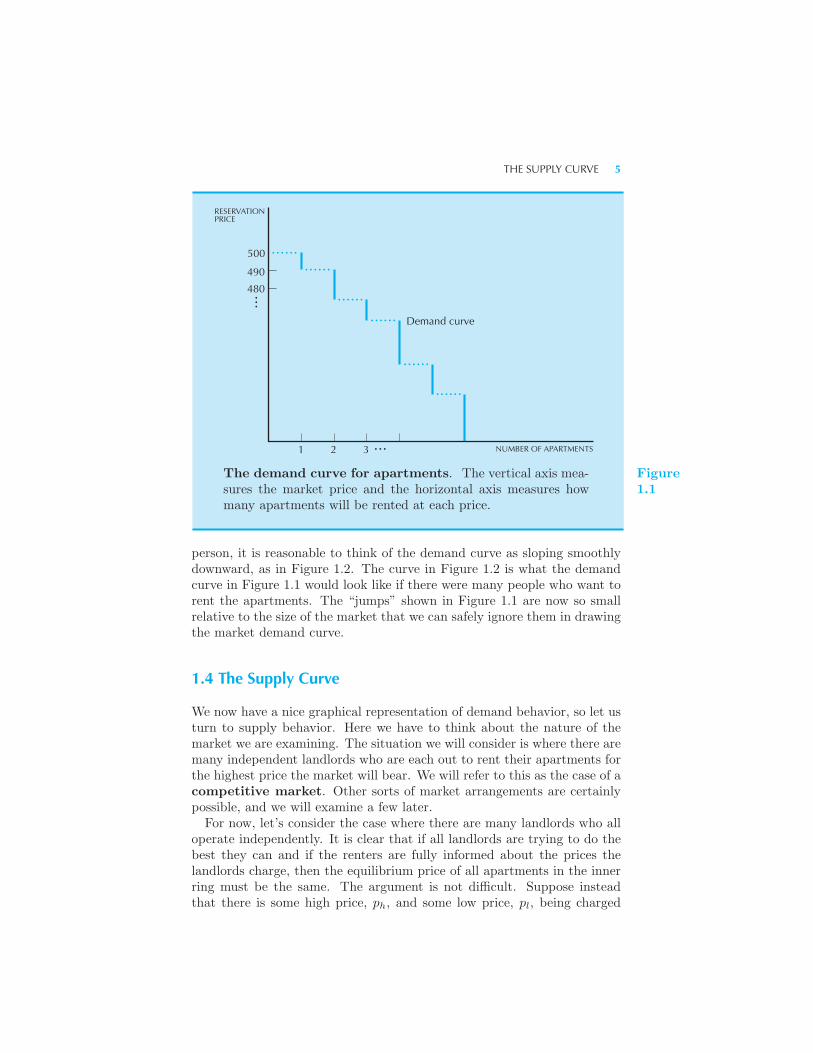
will just be the number of people who have a reservation price greater thanor equal to p∗. For if the market price is p∗, then everyone who is willingto pay at least p∗ for an apartment will want an apartment in the innerring, and everyone who is not willing to pay p∗ will choose to live in theouter ring.We can plot these reservation prices in a diagram as in Figure 1.1. Here
the price is depicted on the vertical axis and the number of people who arewilling to pay that price or more is depicted on the horizontal axis.Another way to view Figure 1.1 is to think of it as measuring how many
people would want to rent apartments at any particular price. Such a curveis an example of a demand curve—a curve that relates the quantitydemanded to price. When the market price is above $500, zero apart-ments will be rented. When the price is between $500 and $490, oneapartment will be rented. When it is between $490 and the third high-est reservation price, two apartments will be rented, and so on. Thedemand curve describes the quantity demanded at each of the possibleprices.The demand curve for apartments slopes down: as the price of apart-
ments decreases more people will be willing to rent apartments. If there aremany people and their reservation prices differ only slightly from person to
THE SUPPLY CURVE 5
......
......
............
............
RESERVATIONPRICE
500
490
480
1 2 3 ...
...
Demand curve
NUMBER OF APARTMENTS
The demand curve for apartments. The vertical axis mea-sures the market price and the horizontal axis measures howmany apartments will be rented at each price.
Figure1.1
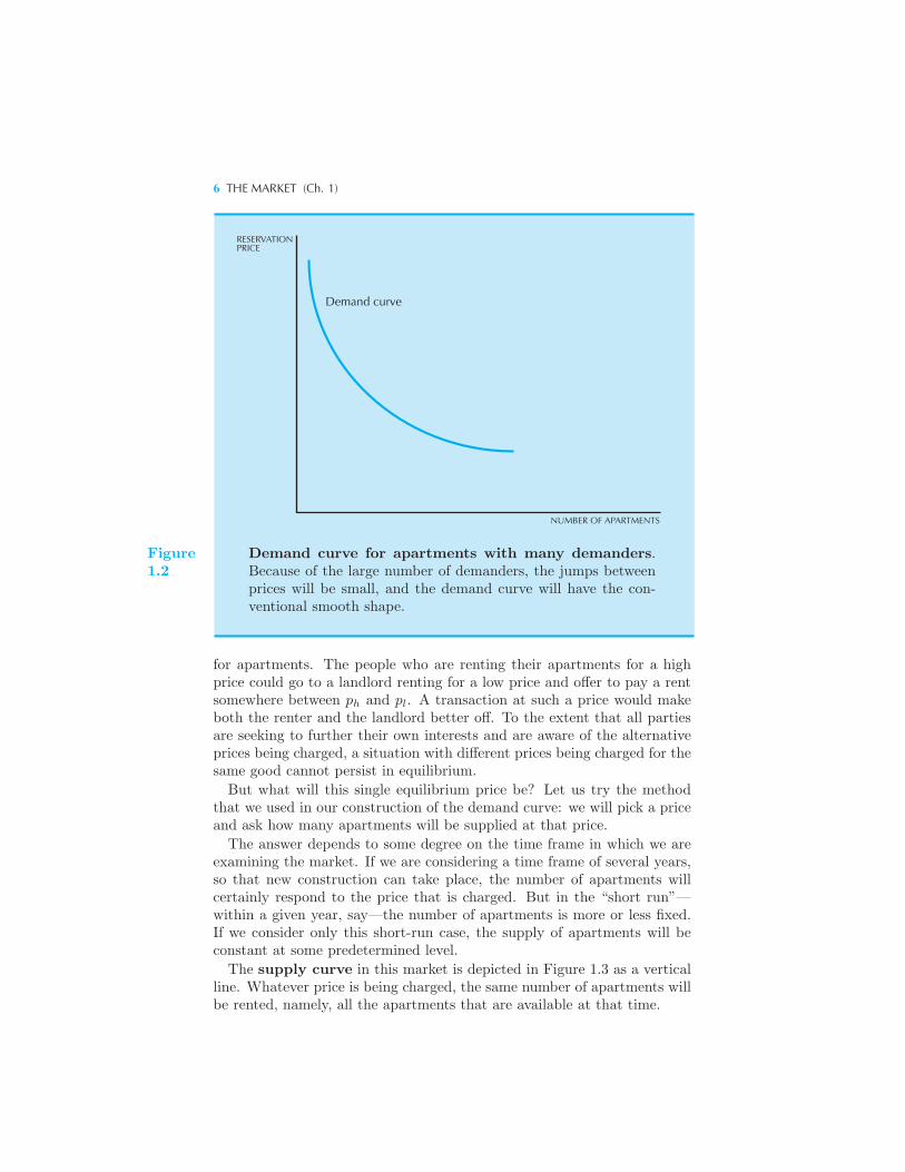
person, it is reasonable to think of the demand curve as sloping smoothlydownward, as in Figure 1.2. The curve in Figure 1.2 is what the demandcurve in Figure 1.1 would look like if there were many people who want torent the apartments. The “jumps” shown in Figure 1.1 are now so smallrelative to the size of the market that we can safely ignore them in drawingthe market demand curve.
1.4 The Supply Curve
We now have a nice graphical representation of demand behavior, so let usturn to supply behavior. Here we have to think about the nature of themarket we are examining. The situation we will consider is where there aremany independent landlords who are each out to rent their apartments forthe highest price the market will bear. We will refer to this as the case of acompetitive market. Other sorts of market arrangements are certainlypossible, and we will examine a few later.For now, let’s consider the case where there are many landlords who all
operate independently. It is clear that if all landlords are trying to do thebest they can and if the renters are fully informed about the prices thelandlords charge, then the equilibrium price of all apartments in the innerring must be the same. The argument is not difficult. Suppose insteadthat there is some high price, ph, and some low price, pl, being charged
6 THE MARKET (Ch. 1)
Demand curve
RESERVATIONPRICE
NUMBER OF APARTMENTS
Figure1.2
Demand curve for apartments with many demanders.Because of the large number of demanders, the jumps betweenprices will be small, and the demand curve will have the con-ventional smooth shape.
for apartments. The people who are renting their apartments for a highprice could go to a landlord renting for a low price and offer to pay a rentsomewhere between ph and pl. A transaction at such a price would makeboth the renter and the landlord better off. To the extent that all partiesare seeking to further their own interests and are aware of the alternativeprices being charged, a situation with different prices being charged for thesame good cannot persist in equilibrium.
But what will this single equilibrium price be? Let us try the methodthat we used in our construction of the demand curve: we will pick a priceand ask how many apartments will be supplied at that price.
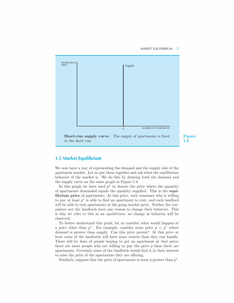
The answer depends to some degree on the time frame in which we areexamining the market. If we are considering a time frame of several years,so that new construction can take place, the number of apartments willcertainly respond to the price that is charged. But in the “short run”—within a given year, say—the number of apartments is more or less fixed.If we consider only this short-run case, the supply of apartments will beconstant at some predetermined level.
The supply curve in this market is depicted in Figure 1.3 as a verticalline. Whatever price is being charged, the same number of apartments willbe rented, namely, all the apartments that are available at that time.
MARKET EQUILIBRIUM 7
RESERVATIONPRICE
NUMBER OF APARTMENTS
Supply
S
Short-run supply curve. The supply of apartments is fixedin the short run.
Figure1.3
1.5 Market Equilibrium
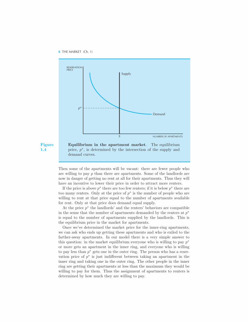
We now have a way of representing the demand and the supply side of theapartment market. Let us put them together and ask what the equilibriumbehavior of the market is. We do this by drawing both the demand andthe supply curve on the same graph in Figure 1.4.In this graph we have used p∗ to denote the price where the quantity
of apartments demanded equals the quantity supplied. This is the equi-librium price of apartments. At this price, each consumer who is willingto pay at least p∗ is able to find an apartment to rent, and each landlordwill be able to rent apartments at the going market price. Neither the con-sumers nor the landlords have any reason to change their behavior. Thisis why we refer to this as an equilibrium: no change in behavior will beobserved.To better understand this point, let us consider what would happen at
a price other than p∗. For example, consider some price p < p∗ wheredemand is greater than supply. Can this price persist? At this price atleast some of the landlords will have more renters than they can handle.There will be lines of people hoping to get an apartment at that price;there are more people who are willing to pay the price p than there areapartments. Certainly some of the landlords would find it in their interestto raise the price of the apartments they are offering.Similarly, suppose that the price of apartments is some p greater than p∗.
8 THE MARKET (Ch. 1)
Supply
Demand
RESERVATIONPRICE
NUMBER OF APARTMENTSS
p*
Figure1.4
Equilibrium in the apartment market. The equilibriumprice, p∗, is determined by the intersection of the supply anddemand curves.
Then some of the apartments will be vacant: there are fewer people whoare willing to pay p than there are apartments. Some of the landlords arenow in danger of getting no rent at all for their apartments. Thus they willhave an incentive to lower their price in order to attract more renters.If the price is above p∗ there are too few renters; if it is below p∗ there are
too many renters. Only at the price of p∗ is the number of people who arewilling to rent at that price equal to the number of apartments availablefor rent. Only at that price does demand equal supply.At the price p∗ the landlords’ and the renters’ behaviors are compatible
in the sense that the number of apartments demanded by the renters at p∗
is equal to the number of apartments supplied by the landlords. This isthe equilibrium price in the market for apartments.Once we’ve determined the market price for the inner-ring apartments,
we can ask who ends up getting these apartments and who is exiled to thefarther-away apartments. In our model there is a very simple answer tothis question: in the market equilibrium everyone who is willing to pay p∗
or more gets an apartment in the inner ring, and everyone who is willingto pay less than p∗ gets one in the outer ring. The person who has a reser-vation price of p∗ is just indifferent between taking an apartment in theinner ring and taking one in the outer ring. The other people in the innerring are getting their apartments at less than the maximum they would bewilling to pay for them. Thus the assignment of apartments to renters isdetermined by how much they are willing to pay.
COMPARATIVE STATICS 9
1.6 Comparative Statics
Now that we have an economic model of the apartment market, we canbegin to use it to analyze the behavior of the equilibrium price. For exam-ple, we can ask how the price of apartments changes when various aspectsof the market change. This kind of an exercise is known as compara-tive statics, because it involves comparing two “static” equilibria withoutworrying about how the market moves from one equilibrium to another.The movement from one equilibrium to another can take a substantial
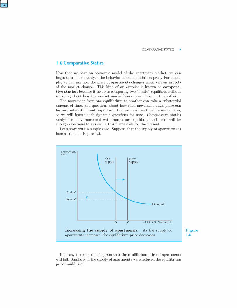
amount of time, and questions about how such movement takes place canbe very interesting and important. But we must walk before we can run,so we will ignore such dynamic questions for now. Comparative staticsanalysis is only concerned with comparing equilibria, and there will beenough questions to answer in this framework for the present.Let’s start with a simple case. Suppose that the supply of apartments is
increased, as in Figure 1.5.
Demand
RESERVATIONPRICE
NUMBER OF APARTMENTS
Oldsupply
Newsupply
S S'
Old p*
New p*
Increasing the supply of apartments. As the supply ofapartments increases, the equilibrium price decreases.
Figure1.5
It is easy to see in this diagram that the equilibrium price of apartmentswill fall. Similarly, if the supply of apartments were reduced the equilibriumprice would rise.
10 THE MARKET (Ch. 1)
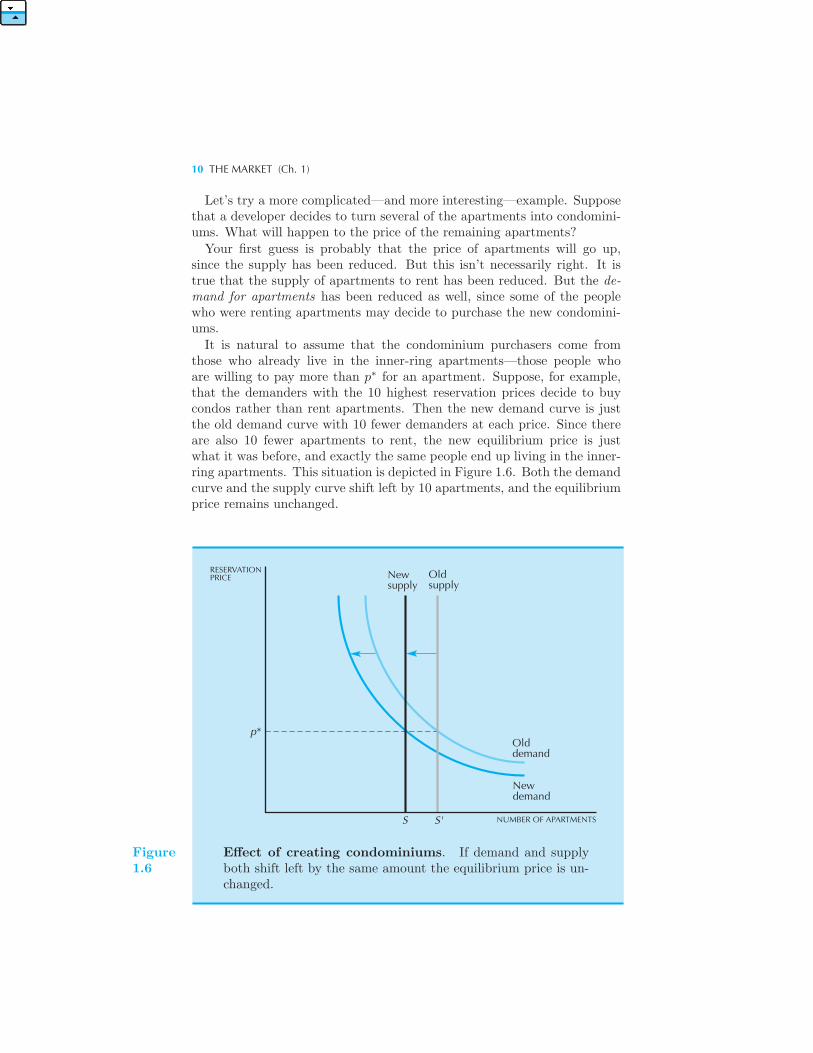
Let’s try a more complicated—and more interesting—example. Supposethat a developer decides to turn several of the apartments into condomini-ums. What will happen to the price of the remaining apartments?
Your first guess is probably that the price of apartments will go up,since the supply has been reduced. But this isn’t necessarily right. It istrue that the supply of apartments to rent has been reduced. But the de-mand for apartments has been reduced as well, since some of the peoplewho were renting apartments may decide to purchase the new condomini-ums.
It is natural to assume that the condominium purchasers come fromthose who already live in the inner-ring apartments—those people whoare willing to pay more than p∗ for an apartment. Suppose, for example,that the demanders with the 10 highest reservation prices decide to buycondos rather than rent apartments. Then the new demand curve is justthe old demand curve with 10 fewer demanders at each price. Since thereare also 10 fewer apartments to rent, the new equilibrium price is justwhat it was before, and exactly the same people end up living in the inner-ring apartments. This situation is depicted in Figure 1.6. Both the demandcurve and the supply curve shift left by 10 apartments, and the equilibriumprice remains unchanged.
RESERVATIONPRICE
NUMBER OF APARTMENTS
Oldsupply
Newsupply
S S'
Olddemand
Newdemand
p*
Figure1.6
Effect of creating condominiums. If demand and supplyboth shift left by the same amount the equilibrium price is un-changed.
OTHER WAYS TO ALLOCATE APARTMENTS 11
Most people find this result surprising. They tend to see just the reduc-tion in the supply of apartments and don’t think about the reduction indemand. The case we’ve considered is an extreme one: all of the condo pur-chasers were former apartment dwellers. But the other case—where noneof the condo purchasers were apartment dwellers—is even more extreme.
The model, simple though it is, has led us to an important insight. If wewant to determine how conversion to condominiums will affect the apart-ment market, we have to consider not only the effect on the supply ofapartments but also the effect on the demand for apartments.
Let’s consider another example of a surprising comparative statics anal-ysis: the effect of an apartment tax. Suppose that the city council decidesthat there should be a tax on apartments of $50 a year. Thus each landlordwill have to pay $50 a year to the city for each apartment that he owns.What will this do to the price of apartments?
Most people would think that at least some of the tax would get passedalong to apartment renters. But, rather surprisingly, that is not the case.In fact, the equilibrium price of apartments will remain unchanged!
In order to verify this, we have to ask what happens to the demand curveand the supply curve. The supply curve doesn’t change—there are just asmany apartments after the tax as before the tax. And the demand curvedoesn’t change either, since the number of apartments that will be rentedat each different price will be the same as well. If neither the demand curvenor the supply curve shifts, the price can’t change as a result of the tax.
Here is a way to think about the effect of this tax. Before the tax isimposed, each landlord is charging the highest price that he can get thatwill keep his apartments occupied. The equilibrium price p∗ is the highestprice that can be charged that is compatible with all of the apartmentsbeing rented. After the tax is imposed can the landlords raise their prices tocompensate for the tax? The answer is no: if they could raise the price andkeep their apartments occupied, they would have already done so. If theywere charging the maximum price that the market could bear, the landlordscouldn’t raise their prices any more: none of the tax can get passed alongto the renters. The landlords have to pay the entire amount of the tax.
This analysis depends on the assumption that the supply of apartmentsremains fixed. If the number of apartments can vary as the tax changes,then the price paid by the renters will typically change. We’ll examine thiskind of behavior later on, after we’ve built up some more powerful toolsfor analyzing such problems.
1.7 Other Ways to Allocate Apartments
In the previous section we described the equilibrium for apartments ina competitive market. But this is only one of many ways to allocate a
12 THE MARKET (Ch. 1)
resource; in this section we describe a few other ways. Some of these maysound rather strange, but each will illustrate an important economic point.
The Discriminating Monopolist
First, let us consider a situation where there is one dominant landlord whoowns all of the apartments. Or, alternatively, we could think of a numberof individual landlords getting together and coordinating their actions toact as one. A situation where a market is dominated by a single seller of aproduct is known as a monopoly.In renting the apartments the landlord could decide to auction them off
one by one to the highest bidders. Since this means that different peoplewould end up paying different prices for apartments, we will call this thecase of the discriminating monopolist. Let us suppose for simplicitythat the discriminating monopolist knows each person’s reservation pricefor apartments. (This is not terribly realistic, but it will serve to illustratean important point.)This means that he would rent the first apartment to the fellow who
would pay the most for it, in this case $500. The next apartment would gofor $490 and so on as we moved down the demand curve. Each apartmentwould be rented to the person who was willing to pay the most for it.Here is the interesting feature of the discriminating monopolist: exactly
the same people will get the apartments as in the case of the market solution,namely, everyone who valued an apartment at more than p∗. The lastperson to rent an apartment pays the price p∗—the same as the equilibriumprice in a competitive market. The discriminating monopolist’s attempt tomaximize his own profits leads to the same allocation of apartments as thesupply and demand mechanism of the competitive market. The amount thepeople pay is different, but who gets the apartments is the same. It turnsout that this is no accident, but we’ll have to wait until later to explainthe reason.
The Ordinary Monopolist
We assumed that the discriminating monopolist was able to rent each apart-ment at a different price. But what if he were forced to rent all apartmentsat the same price? In this case the monopolist faces a tradeoff: if he choosesa low price he will rent more apartments, but he may end up making lessmoney than if he sets a higher price.Let us use D(p) to represent the demand function—the number of apart-
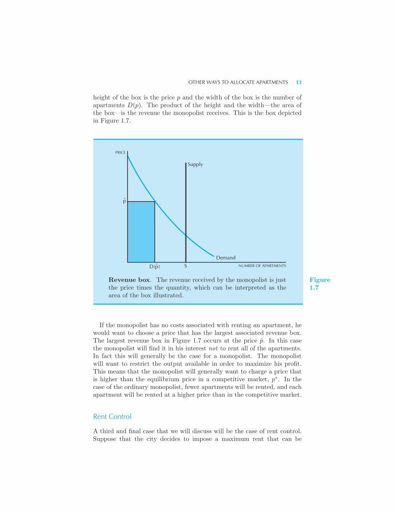
ments demanded at price p. Then if the monopolist sets a price p, he willrent D(p) apartments and thus receive a revenue of pD(p). The revenuethat the monopolist receives can be thought of as the area of a box: the
OTHER WAYS TO ALLOCATE APARTMENTS 13
height of the box is the price p and the width of the box is the number ofapartments D(p). The product of the height and the width—the area ofthe box—is the revenue the monopolist receives. This is the box depictedin Figure 1.7.
Supply
p
DemandNUMBER OF APARTMENTSS
ˆ
D(p)ˆ
PRICE
Revenue box. The revenue received by the monopolist is justthe price times the quantity, which can be interpreted as thearea of the box illustrated.
Figure1.7
If the monopolist has no costs associated with renting an apartment, hewould want to choose a price that has the largest associated revenue box.The largest revenue box in Figure 1.7 occurs at the price p. In this casethe monopolist will find it in his interest not to rent all of the apartments.In fact this will generally be the case for a monopolist. The monopolistwill want to restrict the output available in order to maximize his profit.This means that the monopolist will generally want to charge a price thatis higher than the equilibrium price in a competitive market, p∗. In thecase of the ordinary monopolist, fewer apartments will be rented, and eachapartment will be rented at a higher price than in the competitive market.
Rent Control
A third and final case that we will discuss will be the case of rent control.Suppose that the city decides to impose a maximum rent that can be
14 THE MARKET (Ch. 1)
charged for apartments, say pmax. We suppose that the price pmax is lessthan the equilibrium price in the competitive market, p∗. If this is so wewould have a situation of excess demand: there are more people who arewilling to rent apartments at pmax than there are apartments available.Who will end up with the apartments?The theory that we have described up until now doesn’t have an answer
to this question. We can describe what will happen when supply equalsdemand, but we don’t have enough detail in the model to describe whatwill happen if supply doesn’t equal demand. The answer to who gets theapartments under rent control depends on who has the most time to spendlooking around, who knows the current tenants, and so on. All of thesethings are outside the scope of the simple model we’ve developed. It maybe that exactly the same people get the apartments under rent control asunder the competitive market. But that is an extremely unlikely outcome.It is much more likely that some of the formerly outer-ring people willend up in some of the inner-ring apartments and thus displace the peoplewho would have been living there under the market system. So under rentcontrol the same number of apartments will be rented at the rent-controlledprice as were rented under the competitive price: they’ll just be rented todifferent people.
1.8 Which Way Is Best?
We’ve now described four possible ways of allocating apartments to people:
• The competitive market.• A discriminating monopolist.• An ordinary monopolist.• Rent control.
These are four different economic institutions for allocating apartments.Each method will result in different people getting apartments or in differ-ent prices being charged for apartments. We might well ask which economicinstitution is best. But first we have to define “best.” What criteria mightwe use to compare these ways of allocating apartments?One thing we can do is to look at the economic positions of the people
involved. It is pretty obvious that the owners of the apartments end upwith the most money if they can act as discriminating monopolists: thiswould generate the most revenues for the apartment owner(s). Similarlythe rent-control solution is probably the worst situation for the apartmentowners.What about the renters? They are probably worse off on average in
the case of a discriminating monopolist—most of them would be paying ahigher price than they would under the other ways of allocating apartments.
PARETO EFFICIENCY 15
Are the consumers better off in the case of rent control? Some of them are:the consumers who end up getting the apartments are better off than theywould be under the market solution. But the ones who didn’t get theapartments are worse off than they would be under the market solution.What we need here is a way to look at the economic position of all the
parties involved—all the renters and all the landlords. How can we examinethe desirability of different ways to allocate apartments, taking everybodyinto account? What can be used as a criterion for a “good” way to allocateapartments taking into account all of the parties involved?
1.9 Pareto Efficiency
One useful criterion for comparing the outcomes of different economic insti-tutions is a concept known as Pareto efficiency or economic efficiency.1 Westart with the following definition: if we can find a way to make some peoplebetter off without making anybody else worse off, we have a Pareto im-provement. If an allocation allows for a Pareto improvement, it is calledPareto inefficient; if an allocation is such that no Pareto improvementsare possible, it is called Pareto efficient.
A Pareto inefficient allocation has the undesirable feature that there issome way to make somebody better off without hurting anyone else. Theremay be other positive things about the allocation, but the fact that it isPareto inefficient is certainly one strike against it. If there is a way to makesomeone better off without hurting anyone else, why not do it?The idea of Pareto efficiency is an important one in economics and we
will examine it in some detail later on. It has many subtle implicationsthat we will have to investigate more slowly, but we can get an inkling ofwhat is involved even now.Here is a useful way to think about the idea of Pareto efficiency. Sup-
pose that we assigned the renters to the inner- and outer-ring apartmentsrandomly, but then allowed them to sublet their apartments to each other.Some people who really wanted to live close in might, through bad luck, endup with an outer-ring apartment. But then they could sublet an inner-ringapartment from someone who was assigned to such an apartment but whodidn’t value it as highly as the other person. If individuals were assignedrandomly to apartments, there would generally be some who would wantto trade apartments, if they were sufficiently compensated for doing so.For example, suppose that person A is assigned an apartment in the inner
ring that he feels is worth $200, and that there is some person B in the outerring who would be willing to pay $300 for A’s apartment. Then there is a
1 Pareto efficiency is named after the nineteenth-century economist and sociologistVilfredo Pareto (1848–1923) who was one of the first to examine the implications ofthis idea.
16 THE MARKET (Ch. 1)
“gain from trade” if these two agents swap apartments and arrange a sidepayment from B to A of some amount of money between $200 and $300.The exact amount of the transaction isn’t important. What is importantis that the people who are willing to pay the most for the apartments getthem—otherwise, there would be an incentive for someone who attached alow value to an inner-ring apartment to make a trade with someone whoplaced a high value on an inner-ring apartment.Suppose that we think of all voluntary trades as being carried out so
that all gains from trade are exhausted. The resulting allocation must bePareto efficient. If not, there would be some trade that would make twopeople better off without hurting anyone else—but this would contradictthe assumption that all voluntary trades had been carried out. An alloca-tion in which all voluntary trades have been carried out is a Pareto efficientallocation.
1.10 Comparing Ways to Allocate Apartments
The trading process we’ve described above is so general that you wouldn’tthink that anything much could be said about its outcome. But there isone very interesting point that can be made. Let us ask who will end upwith apartments in an allocation where all of the gains from trade havebeen exhausted.To see the answer, just note that anyone who has an apartment in the
inner ring must have a higher reservation price than anyone who has anapartment in the outer ring—otherwise, they could make a trade and makeboth people better off. Thus if there are S apartments to be rented, thenthe S people with the highest reservation prices end up getting apartmentsin the inner ring. This allocation is Pareto efficient—anything else is not,since any other assignment of apartments to people would allow for sometrade that would make at least two of the people better off without hurtinganyone else.Let us try to apply this criterion of Pareto efficiency to the outcomes of
the various resource allocation devices mentioned above. Let’s start withthe market mechanism. It is easy to see that the market mechanism assignsthe people with the S highest reservation prices to the inner ring—namely,those people who are willing to pay more than the equilibrium price, p∗,for their apartments. Thus there are no further gains from trade to behad once the apartments have been rented in a competitive market. Theoutcome of the competitive market is Pareto efficient.What about the discriminating monopolist? Is that arrangement Pareto
efficient? To answer this question, simply observe that the discriminat-ing monopolist assigns apartments to exactly the same people who receiveapartments in the competitive market. Under each system everyone who iswilling to pay more than p∗ for an apartment gets an apartment. Thus thediscriminating monopolist generates a Pareto efficient outcome as well.
EQUILIBRIUM IN THE LONG RUN 17
Although both the competitive market and the discriminating monop-olist generate Pareto efficient outcomes in the sense that there will be nofurther trades desired, they can result in quite different distributions ofincome. Certainly the consumers are much worse off under the discrimi-nating monopolist than under the competitive market, and the landlord(s)are much better off. In general, Pareto efficiency doesn’t have much to sayabout distribution of the gains from trade. It is only concerned with theefficiency of the trade: whether all of the possible trades have been made.What about the ordinary monopolist who is constrained to charge just
one price? It turns out that this situation is not Pareto efficient. All wehave to do to verify this is to note that, since all the apartments will not ingeneral be rented by the monopolist, he can increase his profits by rentingan apartment to someone who doesn’t have one at any positive price. Thereis some price at which both the monopolist and the renter must be betteroff. As long as the monopolist doesn’t change the price that anybody elsepays, the other renters are just as well off as they were before. Thus wehave found a Pareto improvement—a way to make two parties betteroff without making anyone else worse off.The final case is that of rent control. This also turns out not to be Pareto
efficient. The argument here rests on the fact that an arbitrary assignmentof renters to apartments will generally involve someone living in the innerring (say Mr. In) who is willing to pay less for an apartment than someoneliving in the outer ring (say Ms. Out). Suppose that Mr. In’s reservationprice is $300 and Ms. Out’s reservation price is $500.We need to find a Pareto improvement—a way to make Mr. In and
Ms. Out better off without hurting anyone else. But there is an easy wayto do this: just let Mr. In sublet his apartment to Ms. Out. It is worth $500to Ms. Out to live close to the university, but it is only worth $300 to Mr. In.If Ms. Out pays Mr. In $400, say, and trades apartments, they will both bebetter off: Ms. Out will get an apartment that she values at more than $400,and Mr. In will get $400 that he values more than an inner-ring apartment.This example shows that the rent-controlled market will generally not
result in a Pareto efficient allocation, since there will still be some tradesthat could be carried out after the market has operated. As long as somepeople get inner-ring apartments who value them less highly than peoplewho don’t get them, there will be gains to be had from trade.
1.11 Equilibrium in the Long Run
We have analyzed the equilibrium pricing of apartments in the short run—when there is a fixed supply of apartments. But in the long run the supplyof apartments can change. Just as the demand curve measures the numberof apartments that will be demanded at different prices, the supply curvemeasures the number of apartments that will be supplied at different prices.
18 THE MARKET (Ch. 1)
The final determination of the market price for apartments will depend onthe interaction of supply and demand.And what is it that determines the supply behavior? In general, the
number of new apartments that will be supplied by the private market willdepend on how profitable it is to provide apartments, which depends, inpart, on the price that landlords can charge for apartments. In order toanalyze the behavior of the apartment market in the long run, we haveto examine the behavior of suppliers as well as demanders, a task we willeventually undertake.When supply is variable, we can ask questions not only about who gets
the apartments, but about how many will be provided by various types ofmarket institutions. Will a monopolist supply more or fewer apartmentsthan a competitive market? Will rent control increase or decrease the equi-librium number of apartments? Which institutions will provide a Paretoefficient number of apartments? In order to answer these and similar ques-tions we must develop more systematic and powerful tools for economicanalysis.
Summary
1. Economics proceeds by making models of social phenomena, which aresimplified representations of reality.
2. In this task, economists are guided by the optimization principle, whichstates that people typically try to choose what’s best for them, and by theequilibrium principle, which says that prices will adjust until demand andsupply are equal.
3. The demand curve measures how much people wish to demand at eachprice, and the supply curve measures how much people wish to supply ateach price. An equilibrium price is one where the amount demanded equalsthe amount supplied.
4. The study of how the equilibrium price and quantity change when theunderlying conditions change is known as comparative statics.
5. An economic situation is Pareto efficient if there is no way to make somegroup of people better off without making some other group of people worseoff. The concept of Pareto efficiency can be used to evaluate different waysof allocating resources.
REVIEW QUESTIONS 19
REVIEW QUESTIONS
1. Suppose that there were 25 people who had a reservation price of $500,and the 26th person had a reservation price of $200. What would thedemand curve look like?
2. In the above example, what would the equilibrium price be if there were24 apartments to rent? What if there were 26 apartments to rent? Whatif there were 25 apartments to rent?
3. If people have different reservation prices, why does the market demandcurve slope down?
4. In the text we assumed that the condominium purchasers came fromthe inner-ring people—people who were already renting apartments. Whatwould happen to the price of inner-ring apartments if all of the condo-minium purchasers were outer-ring people—the people who were not cur-rently renting apartments in the inner ring?
5. Suppose now that the condominium purchasers were all inner-ring peo-ple, but that each condominium was constructed from two apartments.What would happen to the price of apartments?
6. What do you suppose the effect of a tax would be on the number ofapartments that would be built in the long run?
7. Suppose the demand curve is D(p) = 100 − 2p. What price would themonopolist set if he had 60 apartments? How many would he rent? Whatprice would he set if he had 40 apartments? How many would he rent?
8. If our model of rent control allowed for unrestricted subletting, whowould end up getting apartments in the inner circle? Would the outcomebe Pareto efficient?
CHAPTER 2
BUDGETCONSTRAINT
The economic theory of the consumer is very simple: economists assumethat consumers choose the best bundle of goods they can afford. To givecontent to this theory, we have to describe more precisely what we mean by“best” and what we mean by “can afford.” In this chapter we will examinehow to describe what a consumer can afford; the next chapter will focus onthe concept of how the consumer determines what is best. We will then beable to undertake a detailed study of the implications of this simple modelof consumer behavior.
2.1 The Budget Constraint
We begin by examining the concept of the budget constraint. Supposethat there is some set of goods from which the consumer can choose. Inreal life there are many goods to consume, but for our purposes it is conve-nient to consider only the case of two goods, since we can then depict theconsumer’s choice behavior graphically.We will indicate the consumer’s consumption bundle by (x1, x2). This
is simply a list of two numbers that tells us how much the consumer is choos-ing to consume of good 1, x1, and how much the consumer is choosing to
TWO GOODS ARE OFTEN ENOUGH 21
consume of good 2, x2. Sometimes it is convenient to denote the consumer’sbundle by a single symbol like X, where X is simply an abbreviation forthe list of two numbers (x1, x2).We suppose that we can observe the prices of the two goods, (p1, p2),
and the amount of money the consumer has to spend, m. Then the budgetconstraint of the consumer can be written as
p1x1 + p2x2 ≤ m. (2.1)
Here p1x1 is the amount of money the consumer is spending on good 1,and p2x2 is the amount of money the consumer is spending on good 2.The budget constraint of the consumer requires that the amount of moneyspent on the two goods be no more than the total amount the consumer hasto spend. The consumer’s affordable consumption bundles are those thatdon’t cost any more than m. We call this set of affordable consumptionbundles at prices (p1, p2) and income m the budget set of the consumer.
2.2 Two Goods Are Often Enough
The two-good assumption is more general than you might think at first,since we can often interpret one of the goods as representing everythingelse the consumer might want to consume.For example, if we are interested in studying a consumer’s demand for
milk, we might let x1 measure his or her consumption of milk in quarts permonth. We can then let x2 stand for everything else the consumer mightwant to consume.When we adopt this interpretation, it is convenient to think of good 2
as being the dollars that the consumer can use to spend on other goods.Under this interpretation the price of good 2 will automatically be 1, sincethe price of one dollar is one dollar. Thus the budget constraint will takethe form
p1x1 + x2 ≤ m. (2.2)
This expression simply says that the amount of money spent on good 1,p1x1, plus the amount of money spent on all other goods, x2, must be nomore than the total amount of money the consumer has to spend, m.
We say that good 2 represents a composite good that stands for ev-erything else that the consumer might want to consume other than good1. Such a composite good is invariably measured in dollars to be spenton goods other than good 1. As far as the algebraic form of the budgetconstraint is concerned, equation (2.2) is just a special case of the formulagiven in equation (2.1), with p2 = 1, so everything that we have to sayabout the budget constraint in general will hold under the composite-goodinterpretation.
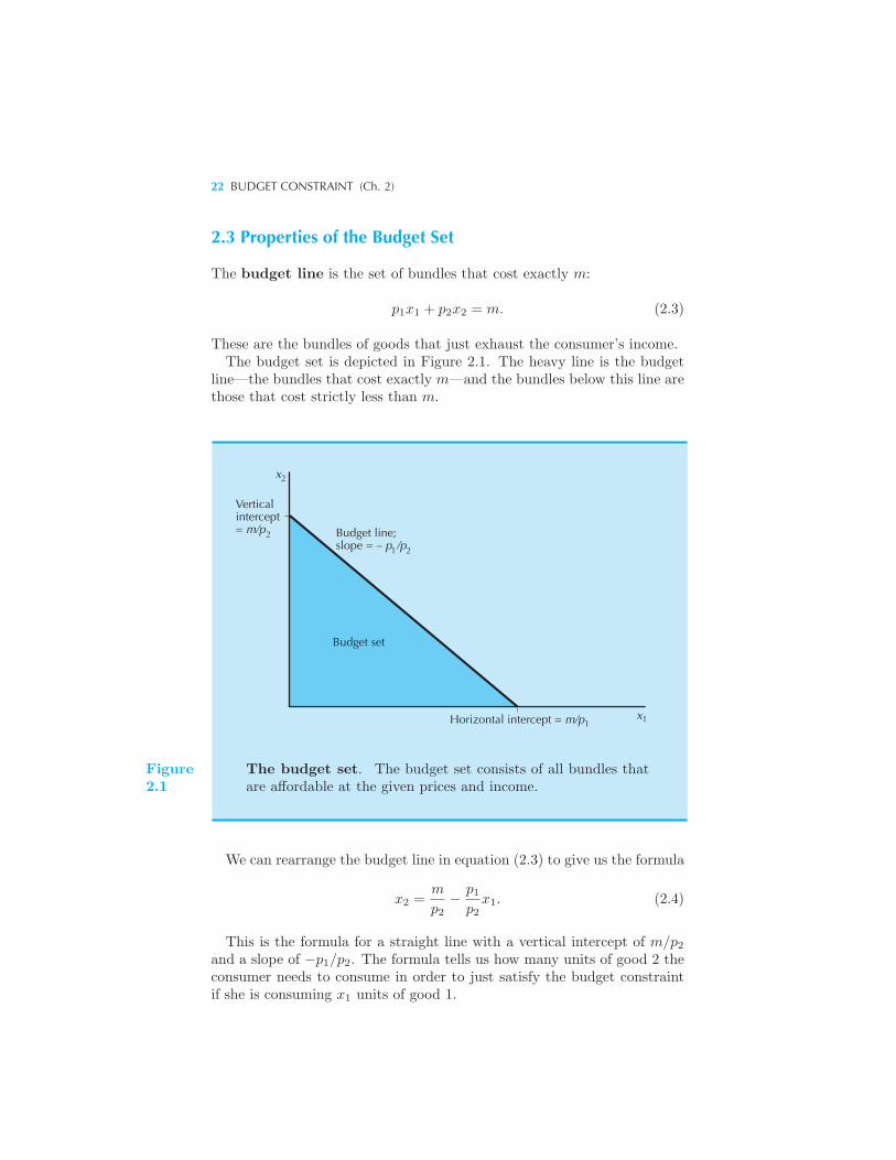
22 BUDGET CONSTRAINT (Ch. 2)
2.3 Properties of the Budget Set
The budget line is the set of bundles that cost exactly m:
p1x1 + p2x2 = m. (2.3)
These are the bundles of goods that just exhaust the consumer’s income.The budget set is depicted in Figure 2.1. The heavy line is the budget
line—the bundles that cost exactly m—and the bundles below this line arethose that cost strictly less than m.
x
Budget line;slope = – p /p
Verticalintercept= m/p2
2
1 2
1 1xHorizontal intercept = m/p
Budget set
Figure2.1
The budget set. The budget set consists of all bundles thatare affordable at the given prices and income.
We can rearrange the budget line in equation (2.3) to give us the formula
x2 =m
p2− p1
p2x1. (2.4)
This is the formula for a straight line with a vertical intercept of m/p2and a slope of −p1/p2. The formula tells us how many units of good 2 theconsumer needs to consume in order to just satisfy the budget constraintif she is consuming x1 units of good 1.
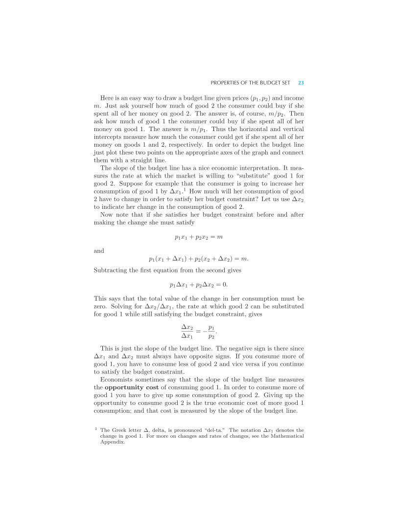
PROPERTIES OF THE BUDGET SET 23
Here is an easy way to draw a budget line given prices (p1, p2) and incomem. Just ask yourself how much of good 2 the consumer could buy if shespent all of her money on good 2. The answer is, of course, m/p2. Thenask how much of good 1 the consumer could buy if she spent all of hermoney on good 1. The answer is m/p1. Thus the horizontal and verticalintercepts measure how much the consumer could get if she spent all of hermoney on goods 1 and 2, respectively. In order to depict the budget linejust plot these two points on the appropriate axes of the graph and connectthem with a straight line.The slope of the budget line has a nice economic interpretation. It mea-
sures the rate at which the market is willing to “substitute” good 1 forgood 2. Suppose for example that the consumer is going to increase herconsumption of good 1 by Δx1.
1 How much will her consumption of good2 have to change in order to satisfy her budget constraint? Let us use Δx2
to indicate her change in the consumption of good 2.Now note that if she satisfies her budget constraint before and after
making the change she must satisfy
p1x1 + p2x2 = m
andp1(x1 +Δx1) + p2(x2 +Δx2) = m.
Subtracting the first equation from the second gives
p1Δx1 + p2Δx2 = 0.
This says that the total value of the change in her consumption must bezero. Solving for Δx2/Δx1, the rate at which good 2 can be substitutedfor good 1 while still satisfying the budget constraint, gives
Δx2
Δx1= −p1
p2.
This is just the slope of the budget line. The negative sign is there sinceΔx1 and Δx2 must always have opposite signs. If you consume more ofgood 1, you have to consume less of good 2 and vice versa if you continueto satisfy the budget constraint.Economists sometimes say that the slope of the budget line measures
the opportunity cost of consuming good 1. In order to consume more ofgood 1 you have to give up some consumption of good 2. Giving up theopportunity to consume good 2 is the true economic cost of more good 1consumption; and that cost is measured by the slope of the budget line.
1 The Greek letter Δ, delta, is pronounced “del-ta.” The notation Δx1 denotes thechange in good 1. For more on changes and rates of changes, see the MathematicalAppendix.
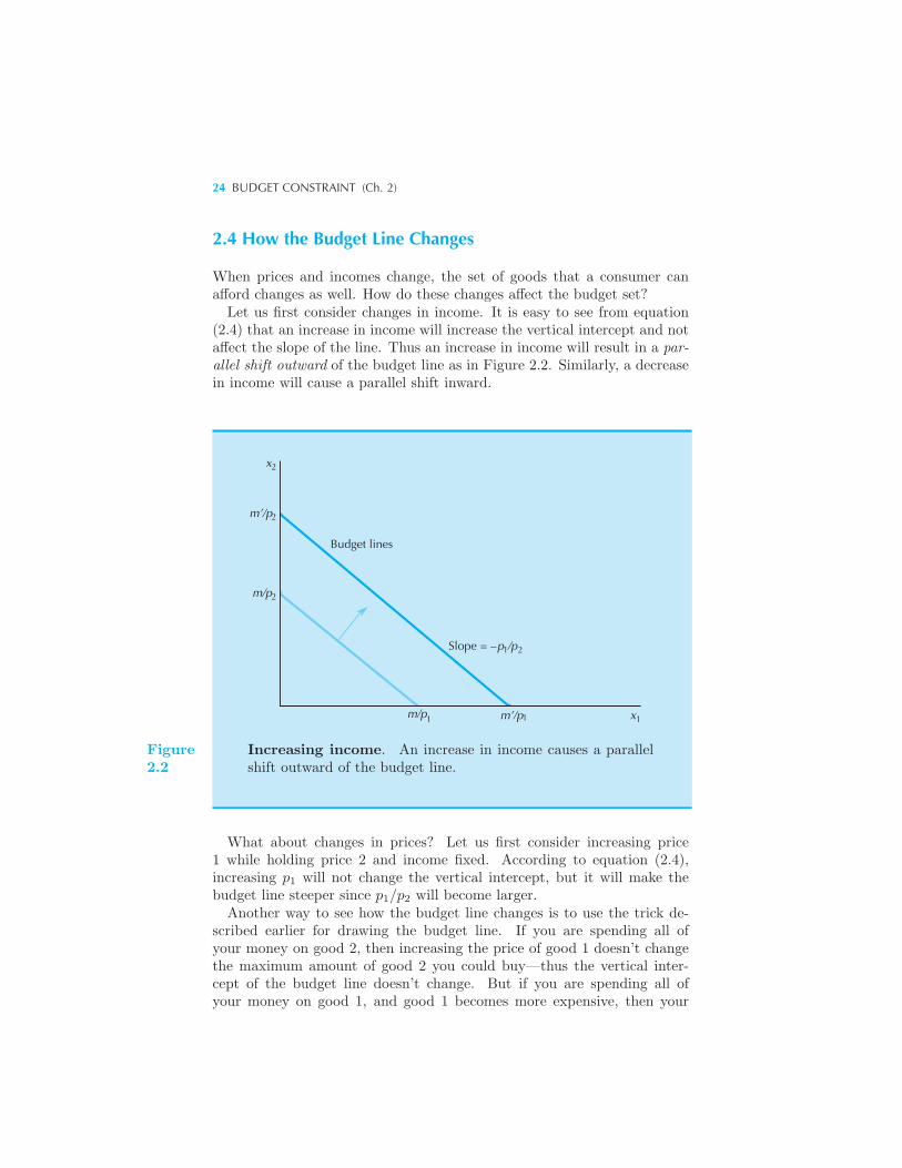
24 BUDGET CONSTRAINT (Ch. 2)
2.4 How the Budget Line Changes
When prices and incomes change, the set of goods that a consumer canafford changes as well. How do these changes affect the budget set?Let us first consider changes in income. It is easy to see from equation
(2.4) that an increase in income will increase the vertical intercept and notaffect the slope of the line. Thus an increase in income will result in a par-allel shift outward of the budget line as in Figure 2.2. Similarly, a decreasein income will cause a parallel shift inward.
Budget lines
1x1m/p 1m’/p
Slope = –p /p21
m/p2
x2
m’/p2
Figure2.2
Increasing income. An increase in income causes a parallelshift outward of the budget line.
What about changes in prices? Let us first consider increasing price1 while holding price 2 and income fixed. According to equation (2.4),increasing p1 will not change the vertical intercept, but it will make thebudget line steeper since p1/p2 will become larger.
Another way to see how the budget line changes is to use the trick de-scribed earlier for drawing the budget line. If you are spending all ofyour money on good 2, then increasing the price of good 1 doesn’t changethe maximum amount of good 2 you could buy—thus the vertical inter-cept of the budget line doesn’t change. But if you are spending all ofyour money on good 1, and good 1 becomes more expensive, then your
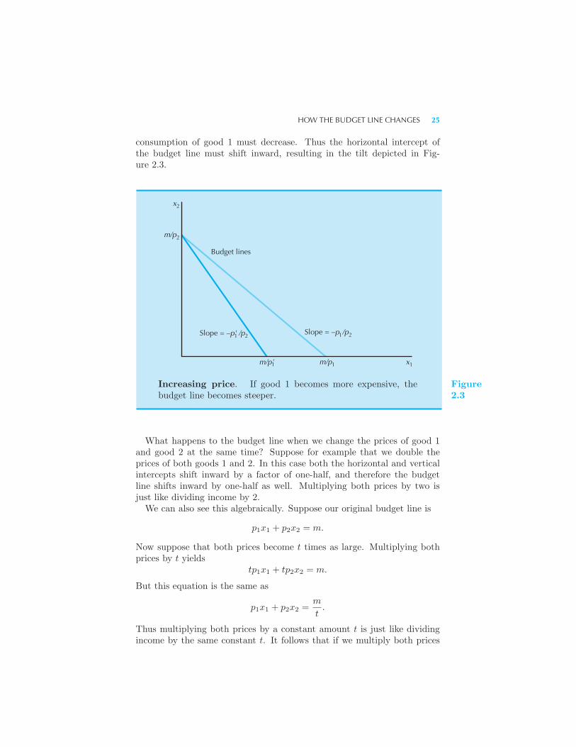
HOW THE BUDGET LINE CHANGES 25
consumption of good 1 must decrease. Thus the horizontal intercept ofthe budget line must shift inward, resulting in the tilt depicted in Fig-ure 2.3.
Slope = –p' /p
Budget lines
Slope = –p /p
m/p
x2
2
2 211
1 1 1xm/pm/p'
Increasing price. If good 1 becomes more expensive, thebudget line becomes steeper.
Figure2.3
What happens to the budget line when we change the prices of good 1and good 2 at the same time? Suppose for example that we double theprices of both goods 1 and 2. In this case both the horizontal and verticalintercepts shift inward by a factor of one-half, and therefore the budgetline shifts inward by one-half as well. Multiplying both prices by two isjust like dividing income by 2.We can also see this algebraically. Suppose our original budget line is
p1x1 + p2x2 = m.
Now suppose that both prices become t times as large. Multiplying bothprices by t yields
tp1x1 + tp2x2 = m.
But this equation is the same as
p1x1 + p2x2 =m
t.
Thus multiplying both prices by a constant amount t is just like dividingincome by the same constant t. It follows that if we multiply both prices
26 BUDGET CONSTRAINT (Ch. 2)
by t and we multiply income by t, then the budget line won’t change atall.We can also consider price and income changes together. What happens
if both prices go up and income goes down? Think about what happens tothe horizontal and vertical intercepts. If m decreases and p1 and p2 bothincrease, then the intercepts m/p1 and m/p2 must both decrease. Thismeans that the budget line will shift inward. What about the slope ofthe budget line? If price 2 increases more than price 1, so that −p1/p2decreases (in absolute value), then the budget line will be flatter; if price 2increases less than price 1, the budget line will be steeper.
2.5 The Numeraire
The budget line is defined by two prices and one income, but one of thesevariables is redundant. We could peg one of the prices, or the income, tosome fixed value, and adjust the other variables so as to describe exactlythe same budget set. Thus the budget line
p1x1 + p2x2 = m
is exactly the same budget line as
p1p2
x1 + x2 =m
p2
orp1m
x1 +p2m
x2 = 1,
since the first budget line results from dividing everything by p2, and thesecond budget line results from dividing everything by m. In the first case,we have pegged p2 = 1, and in the second case, we have pegged m = 1.Pegging the price of one of the goods or income to 1 and adjusting theother price and income appropriately doesn’t change the budget set at all.When we set one of the prices to 1, as we did above, we often refer to that
price as the numeraire price. The numeraire price is the price relative towhich we are measuring the other price and income. It will occasionally beconvenient to think of one of the goods as being a numeraire good, sincethere will then be one less price to worry about.
2.6 Taxes, Subsidies, and Rationing
Economic policy often uses tools that affect a consumer’s budget constraint,such as taxes. For example, if the government imposes a quantity tax, thismeans that the consumer has to pay a certain amount to the government
TAXES, SUBSIDIES, AND RATIONING 27
for each unit of the good he purchases. In the U.S., for example, we payabout 15 cents a gallon as a federal gasoline tax.How does a quantity tax affect the budget line of a consumer? From
the viewpoint of the consumer the tax is just like a higher price. Thus aquantity tax of t dollars per unit of good 1 simply changes the price of good1 from p1 to p1 + t. As we’ve seen above, this implies that the budget linemust get steeper.Another kind of tax is a value tax. As the name implies this is a tax
on the value—the price—of a good, rather than the quantity purchased ofa good. A value tax is usually expressed in percentage terms. Most statesin the U.S. have sales taxes. If the sales tax is 6 percent, then a good thatis priced at $1 will actually sell for $1.06. (Value taxes are also known asad valorem taxes.)If good 1 has a price of p1 but is subject to a sales tax at rate τ , then
the actual price facing the consumer is (1 + τ)p1.2 The consumer has to
pay p1 to the supplier and τp1 to the government for each unit of the goodso the total cost of the good to the consumer is (1 + τ)p1.
A subsidy is the opposite of a tax. In the case of a quantity subsidy,the government gives an amount to the consumer that depends on theamount of the good purchased. If, for example, the consumption of milkwere subsidized, the government would pay some amount of money to eachconsumer of milk depending on the amount that consumer purchased. Ifthe subsidy is s dollars per unit of consumption of good 1, then from theviewpoint of the consumer, the price of good 1 would be p1−s. This wouldtherefore make the budget line flatter.Similarly an ad valorem subsidy is a subsidy based on the price of the
good being subsidized. If the government gives you back $1 for every $2you donate to charity, then your donations to charity are being subsidizedat a rate of 50 percent. In general, if the price of good 1 is p1 and good 1 issubject to an ad valorem subsidy at rate σ, then the actual price of good 1facing the consumer is (1− σ)p1.
3
You can see that taxes and subsidies affect prices in exactly the sameway except for the algebraic sign: a tax increases the price to the consumer,and a subsidy decreases it.Another kind of tax or subsidy that the government might use is a lump-
sum tax or subsidy. In the case of a tax, this means that the governmenttakes away some fixed amount of money, regardless of the individual’s be-havior. Thus a lump-sum tax means that the budget line of a consumerwill shift inward because his money income has been reduced. Similarly, alump-sum subsidy means that the budget line will shift outward. Quantity
2 The Greek letter τ , tau, rhymes with “wow” in mathematical discourse, though mod-ern Greeks pronounce it “taf.”
3 The Greek letter σ is pronounced “sig-ma.”
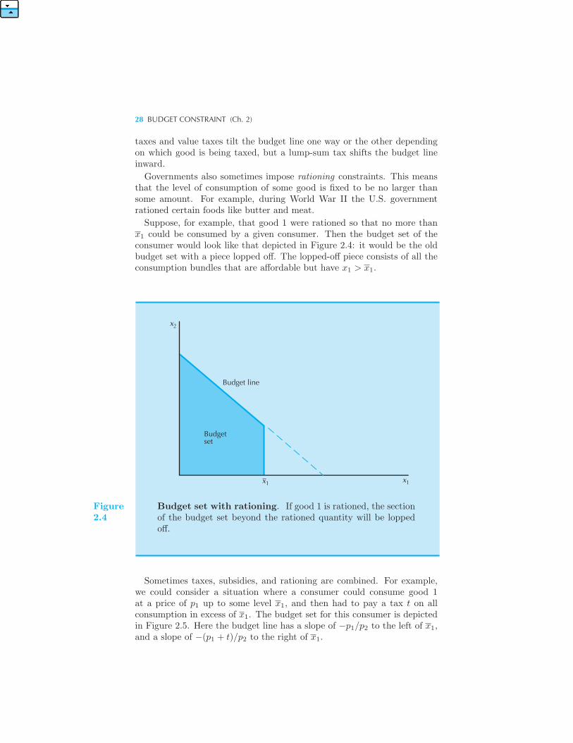
28 BUDGET CONSTRAINT (Ch. 2)
taxes and value taxes tilt the budget line one way or the other dependingon which good is being taxed, but a lump-sum tax shifts the budget lineinward.
Governments also sometimes impose rationing constraints. This meansthat the level of consumption of some good is fixed to be no larger thansome amount. For example, during World War II the U.S. governmentrationed certain foods like butter and meat.
Suppose, for example, that good 1 were rationed so that no more thanx1 could be consumed by a given consumer. Then the budget set of theconsumer would look like that depicted in Figure 2.4: it would be the oldbudget set with a piece lopped off. The lopped-off piece consists of all theconsumption bundles that are affordable but have x1 > x1.
x2
x1 x1
Budget line
Budgetset
Figure2.4
Budget set with rationing. If good 1 is rationed, the sectionof the budget set beyond the rationed quantity will be loppedoff.
Sometimes taxes, subsidies, and rationing are combined. For example,we could consider a situation where a consumer could consume good 1at a price of p1 up to some level x1, and then had to pay a tax t on allconsumption in excess of x1. The budget set for this consumer is depictedin Figure 2.5. Here the budget line has a slope of −p1/p2 to the left of x1,and a slope of −(p1 + t)/p2 to the right of x1.
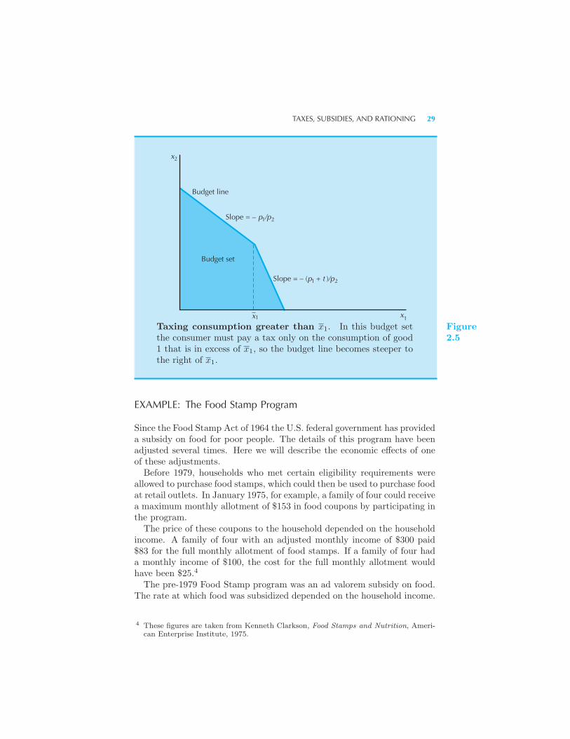
TAXES, SUBSIDIES, AND RATIONING 29
Budget line
Slope = – p /p
x
xx
Slope = – (p + t )/p
1 2
1 2
1 1
2
Budget set
Taxing consumption greater than x1. In this budget setthe consumer must pay a tax only on the consumption of good1 that is in excess of x1, so the budget line becomes steeper tothe right of x1.
Figure2.5
EXAMPLE: The Food Stamp Program
Since the Food Stamp Act of 1964 the U.S. federal government has provideda subsidy on food for poor people. The details of this program have beenadjusted several times. Here we will describe the economic effects of oneof these adjustments.Before 1979, households who met certain eligibility requirements were
allowed to purchase food stamps, which could then be used to purchase foodat retail outlets. In January 1975, for example, a family of four could receivea maximum monthly allotment of $153 in food coupons by participating inthe program.The price of these coupons to the household depended on the household
income. A family of four with an adjusted monthly income of $300 paid$83 for the full monthly allotment of food stamps. If a family of four hada monthly income of $100, the cost for the full monthly allotment wouldhave been $25.4
The pre-1979 Food Stamp program was an ad valorem subsidy on food.The rate at which food was subsidized depended on the household income.
4 These figures are taken from Kenneth Clarkson, Food Stamps and Nutrition, Ameri-can Enterprise Institute, 1975.
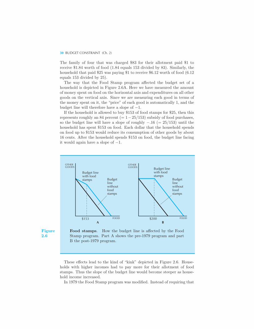
30 BUDGET CONSTRAINT (Ch. 2)
The family of four that was charged $83 for their allotment paid $1 toreceive $1.84 worth of food (1.84 equals 153 divided by 83). Similarly, thehousehold that paid $25 was paying $1 to receive $6.12 worth of food (6.12equals 153 divided by 25).The way that the Food Stamp program affected the budget set of a
household is depicted in Figure 2.6A. Here we have measured the amountof money spent on food on the horizontal axis and expenditures on all othergoods on the vertical axis. Since we are measuring each good in terms ofthe money spent on it, the “price” of each good is automatically 1, and thebudget line will therefore have a slope of −1.If the household is allowed to buy $153 of food stamps for $25, then this
represents roughly an 84 percent (= 1−25/153) subsidy of food purchases,so the budget line will have a slope of roughly −.16 (= 25/153) until thehousehold has spent $153 on food. Each dollar that the household spendson food up to $153 would reduce its consumption of other goods by about16 cents. After the household spends $153 on food, the budget line facingit would again have a slope of −1.
FOOD $200
OTHERGOODS Budget line
with foodstamps
Budgetlinewithoutfoodstamps
Budgetlinewithoutfoodstamps
Budget linewith foodstamps
OTHERGOODS
$153 FOOD
A B
Figure2.6
Food stamps. How the budget line is affected by the FoodStamp program. Part A shows the pre-1979 program and partB the post-1979 program.
These effects lead to the kind of “kink” depicted in Figure 2.6. House-holds with higher incomes had to pay more for their allotment of foodstamps. Thus the slope of the budget line would become steeper as house-hold income increased.In 1979 the Food Stamp program was modified. Instead of requiring that
SUMMARY 31
households purchase food stamps, they are now simply given to qualifiedhouseholds. Figure 2.6B shows how this affects the budget set.Suppose that a household now receives a grant of $200 of food stamps a
month. Then this means that the household can consume $200 more foodper month, regardless of how much it is spending on other goods, whichimplies that the budget line will shift to the right by $200. The slopewill not change: $1 less spent on food would mean $1 more to spend onother things. But since the household cannot legally sell food stamps, themaximum amount that it can spend on other goods does not change. TheFood Stamp program is effectively a lump-sum subsidy, except for the factthat the food stamps can’t be sold.
2.7 Budget Line Changes
In the next chapter we will analyze how the consumer chooses an optimalconsumption bundle from his or her budget set. But we can already statesome observations here that follow from what we have learned about themovements of the budget line.First, we can observe that since the budget set doesn’t change when we
multiply all prices and income by a positive number, the optimal choice ofthe consumer from the budget set can’t change either. Without even ana-lyzing the choice process itself, we have derived an important conclusion:a perfectly balanced inflation—one in which all prices and all incomes riseat the same rate—doesn’t change anybody’s budget set, and thus cannotchange anybody’s optimal choice.Second, we can make some statements about how well-off the consumer
can be at different prices and incomes. Suppose that the consumer’s incomeincreases and all prices remain the same. We know that this represents aparallel shift outward of the budget line. Thus every bundle the consumerwas consuming at the lower income is also a possible choice at the higherincome. But then the consumer must be at least as well-off at the higherincome as at the lower income—since he or she has the same choices avail-able as before plus some more. Similarly, if one price declines and all othersstay the same, the consumer must be at least as well-off. This simple ob-servation will be of considerable use later on.
Summary
1. The budget set consists of all bundles of goods that the consumer canafford at given prices and income. We will typically assume that there areonly two goods, but this assumption is more general than it seems.
2. The budget line is written as p1x1+p2x2 = m. It has a slope of −p1/p2,a vertical intercept of m/p2, and a horizontal intercept of m/p1.

32 BUDGET CONSTRAINT (Ch. 2)
3. Increasing income shifts the budget line outward. Increasing the priceof good 1 makes the budget line steeper. Increasing the price of good 2makes the budget line flatter.
4. Taxes, subsidies, and rationing change the slope and position of thebudget line by changing the prices paid by the consumer.
REVIEW QUESTIONS
1. Originally the consumer faces the budget line p1x1 + p2x2 = m. Thenthe price of good 1 doubles, the price of good 2 becomes 8 times larger,and income becomes 4 times larger. Write down an equation for the newbudget line in terms of the original prices and income.
2. What happens to the budget line if the price of good 2 increases, butthe price of good 1 and income remain constant?
3. If the price of good 1 doubles and the price of good 2 triples, does thebudget line become flatter or steeper?
4. What is the definition of a numeraire good?
5. Suppose that the government puts a tax of 15 cents a gallon on gasolineand then later decides to put a subsidy on gasoline at a rate of 7 cents agallon. What net tax is this combination equivalent to?
6. Suppose that a budget equation is given by p1x1 + p2x2 = m. Thegovernment decides to impose a lump-sum tax of u, a quantity tax ongood 1 of t, and a quantity subsidy on good 2 of s. What is the formulafor the new budget line?
7. If the income of the consumer increases and one of the prices decreasesat the same time, will the consumer necessarily be at least as well-off?
CHAPTER 3
PREFERENCES
We saw in Chapter 2 that the economic model of consumer behavior is verysimple: people choose the best things they can afford. The last chapter wasdevoted to clarifying the meaning of “can afford,” and this chapter will bedevoted to clarifying the economic concept of “best things.”We call the objects of consumer choice consumption bundles. This
is a complete list of the goods and services that are involved in the choiceproblem that we are investigating. The word “complete” deserves empha-sis: when you analyze a consumer’s choice problem, make sure that youinclude all of the appropriate goods in the definition of the consumptionbundle.If we are analyzing consumer choice at the broadest level, we would want
not only a complete list of the goods that a consumer might consume, butalso a description of when, where, and under what circumstances theywould become available. After all, people care about how much food theywill have tomorrow as well as how much food they have today. A raft in themiddle of the Atlantic Ocean is very different from a raft in the middle ofthe Sahara Desert. And an umbrella when it is raining is quite a differentgood from an umbrella on a sunny day. It is often useful to think of the
34 PREFERENCES (Ch. 3)
“same” good available in different locations or circumstances as a differentgood, since the consumer may value the good differently in those situations.However, when we limit our attention to a simple choice problem, the
relevant goods are usually pretty obvious. We’ll often adopt the idea de-scribed earlier of using just two goods and calling one of them “all othergoods” so that we can focus on the tradeoff between one good and ev-erything else. In this way we can consider consumption choices involvingmany goods and still use two-dimensional diagrams.So let us take our consumption bundle to consist of two goods, and let
x1 denote the amount of one good and x2 the amount of the other. Thecomplete consumption bundle is therefore denoted by (x1, x2). As notedbefore, we will occasionally abbreviate this consumption bundle by X.
3.1 Consumer Preferences
We will suppose that given any two consumption bundles, (x1, x2) and(y1, y2), the consumer can rank them as to their desirability. That is, theconsumer can determine that one of the consumption bundles is strictlybetter than the other, or decide that she is indifferent between the twobundles.We will use the symbol � to mean that one bundle is strictly preferred
to another, so that (x1, x2) � (y1, y2) should be interpreted as saying thatthe consumer strictly prefers (x1, x2) to (y1, y2), in the sense that shedefinitely wants the x-bundle rather than the y-bundle. This preferencerelation is meant to be an operational notion. If the consumer prefersone bundle to another, it means that he or she would choose one over theother, given the opportunity. Thus the idea of preference is based on theconsumer’s behavior. In order to tell whether one bundle is preferred toanother, we see how the consumer behaves in choice situations involvingthe two bundles. If she always chooses (x1, x2) when (y1, y2) is available,then it is natural to say that this consumer prefers (x1, x2) to (y1, y2).If the consumer is indifferent between two bundles of goods, we use
the symbol ∼ and write (x1, x2) ∼ (y1, y2). Indifference means that theconsumer would be just as satisfied, according to her own preferences,consuming the bundle (x1, x2) as she would be consuming the other bundle,(y1, y2).If the consumer prefers or is indifferent between the two bundles we say
that she weakly prefers (x1, x2) to (y1, y2) and write (x1, x2) � (y1, y2).These relations of strict preference, weak preference, and indifference
are not independent concepts; the relations are themselves related! Forexample, if (x1, x2) � (y1, y2) and (y1, y2) � (x1, x2) we can conclude that(x1, x2) ∼ (y1, y2). That is, if the consumer thinks that (x1, x2) is at leastas good as (y1, y2) and that (y1, y2) is at least as good as (x1, x2), then theconsumer must be indifferent between the two bundles of goods.

ASSUMPTIONS ABOUT PREFERENCES 35
Similarly, if (x1, x2) � (y1, y2) but we know that it is not the case that(x1, x2) ∼ (y1, y2), we can conclude that we must have (x1, x2) � (y1, y2).This just says that if the consumer thinks that (x1, x2) is at least as goodas (y1, y2), and she is not indifferent between the two bundles, then it mustbe that she thinks that (x1, x2) is strictly better than (y1, y2).
3.2 Assumptions about Preferences
Economists usually make some assumptions about the “consistency” ofconsumers’ preferences. For example, it seems unreasonable—not to saycontradictory—to have a situation where (x1, x2) � (y1, y2) and, at thesame time, (y1, y2) � (x1, x2). For this would mean that the consumerstrictly prefers the x-bundle to the y-bundle . . . and vice versa.So we usually make some assumptions about how the preference relations
work. Some of the assumptions about preferences are so fundamental thatwe can refer to them as “axioms” of consumer theory. Here are three suchaxioms about consumer preference.
Complete. We assume that any two different bundles can be compared.That is, given any x-bundle and any y-bundle, we assume that (x1, x2) �(y1, y2), or (y1, y2) � (x1, x2), or both, in which case the consumer isindifferent between the two bundles.
Reflexive. We assume that any bundle is at least as good as itself:(x1, x2) � (x1, x2).
Transitive. If (x1, x2) � (y1, y2) and (y1, y2) � (z1, z2), then we assumethat (x1, x2) � (z1, z2). In other words, if the consumer thinks that X is atleast as good as Y and that Y is at least as good as Z, then the consumerthinks that X is at least as good as Z.
The first axiom, completeness, is hardly objectionable, at least for thekinds of choices economists generally examine. To say that any two bundlescan be compared is simply to say that the consumer is able to make a choicebetween any two given bundles. One might imagine extreme situationsinvolving life or death choices where ranking the alternatives might bedifficult, or even impossible, but these choices are, for the most part, outsidethe domain of economic analysis.The second axiom, reflexivity, is trivial. Any bundle is certainly at least
as good as an identical bundle. Parents of small children may occasionallyobserve behavior that violates this assumption, but it seems plausible formost adult behavior.The third axiom, transitivity, is more problematic. It isn’t clear that
transitivity of preferences is necessarily a property that preferences wouldhave to have. The assumption that preferences are transitive doesn’t seem
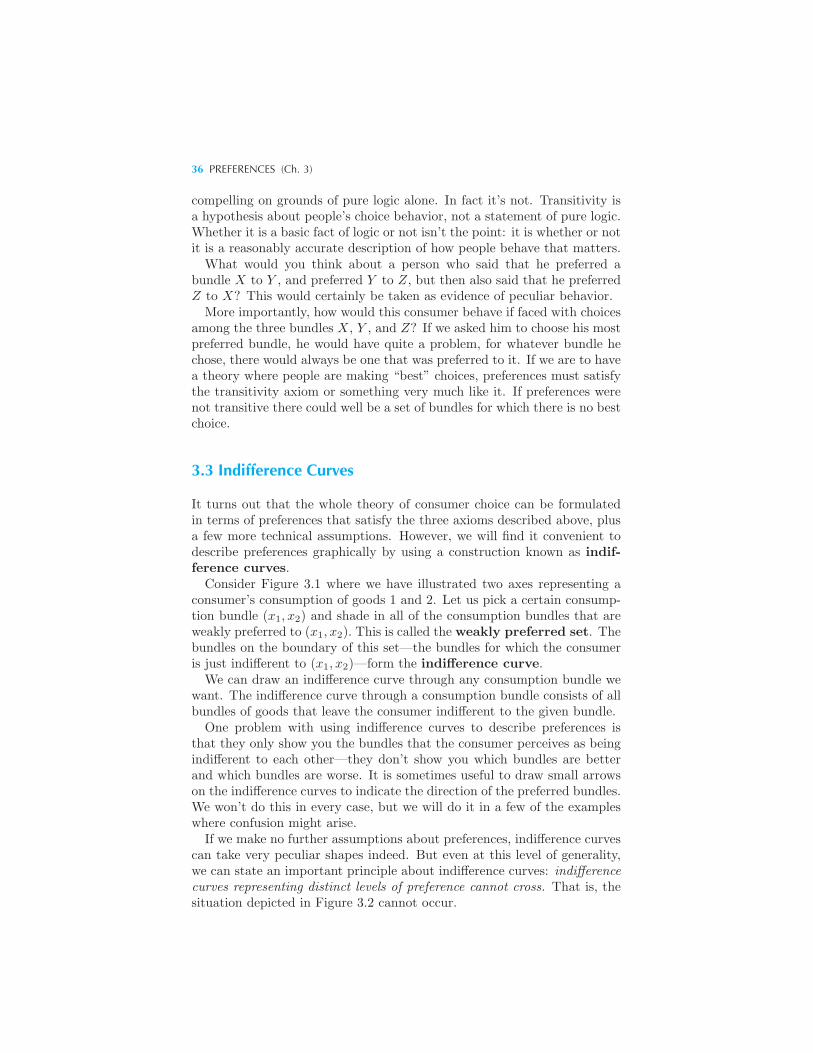
36 PREFERENCES (Ch. 3)
compelling on grounds of pure logic alone. In fact it’s not. Transitivity isa hypothesis about people’s choice behavior, not a statement of pure logic.Whether it is a basic fact of logic or not isn’t the point: it is whether or notit is a reasonably accurate description of how people behave that matters.What would you think about a person who said that he preferred a
bundle X to Y , and preferred Y to Z, but then also said that he preferredZ to X? This would certainly be taken as evidence of peculiar behavior.
More importantly, how would this consumer behave if faced with choicesamong the three bundles X, Y , and Z? If we asked him to choose his mostpreferred bundle, he would have quite a problem, for whatever bundle hechose, there would always be one that was preferred to it. If we are to havea theory where people are making “best” choices, preferences must satisfythe transitivity axiom or something very much like it. If preferences werenot transitive there could well be a set of bundles for which there is no bestchoice.
3.3 Indifference Curves
It turns out that the whole theory of consumer choice can be formulatedin terms of preferences that satisfy the three axioms described above, plusa few more technical assumptions. However, we will find it convenient todescribe preferences graphically by using a construction known as indif-ference curves.
Consider Figure 3.1 where we have illustrated two axes representing aconsumer’s consumption of goods 1 and 2. Let us pick a certain consump-tion bundle (x1, x2) and shade in all of the consumption bundles that areweakly preferred to (x1, x2). This is called the weakly preferred set. Thebundles on the boundary of this set—the bundles for which the consumeris just indifferent to (x1, x2)—form the indifference curve.We can draw an indifference curve through any consumption bundle we
want. The indifference curve through a consumption bundle consists of allbundles of goods that leave the consumer indifferent to the given bundle.One problem with using indifference curves to describe preferences is
that they only show you the bundles that the consumer perceives as beingindifferent to each other—they don’t show you which bundles are betterand which bundles are worse. It is sometimes useful to draw small arrowson the indifference curves to indicate the direction of the preferred bundles.We won’t do this in every case, but we will do it in a few of the exampleswhere confusion might arise.If we make no further assumptions about preferences, indifference curves
can take very peculiar shapes indeed. But even at this level of generality,we can state an important principle about indifference curves: indifferencecurves representing distinct levels of preference cannot cross. That is, thesituation depicted in Figure 3.2 cannot occur.
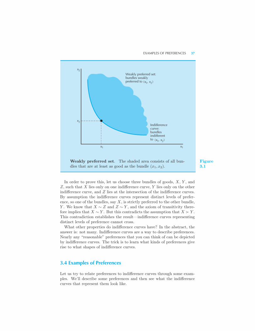
EXAMPLES OF PREFERENCES 37
x2
Weakly preferred set:bundles weaklypreferred to
Indifferencecurve:bundlesindifferentto
x1
(x , x )1 2
1x
2x
(x , x )21
Weakly preferred set. The shaded area consists of all bun-dles that are at least as good as the bundle (x1, x2).
Figure3.1
In order to prove this, let us choose three bundles of goods, X, Y , andZ, such that X lies only on one indifference curve, Y lies only on the otherindifference curve, and Z lies at the intersection of the indifference curves.By assumption the indifference curves represent distinct levels of prefer-ence, so one of the bundles, say X, is strictly preferred to the other bundle,Y . We know that X ∼ Z and Z ∼ Y , and the axiom of transitivity there-fore implies that X ∼ Y . But this contradicts the assumption that X � Y .This contradiction establishes the result—indifference curves representingdistinct levels of preference cannot cross.What other properties do indifference curves have? In the abstract, the
answer is: not many. Indifference curves are a way to describe preferences.Nearly any “reasonable” preferences that you can think of can be depictedby indifference curves. The trick is to learn what kinds of preferences giverise to what shapes of indifference curves.
3.4 Examples of Preferences
Let us try to relate preferences to indifference curves through some exam-ples. We’ll describe some preferences and then see what the indifferencecurves that represent them look like.
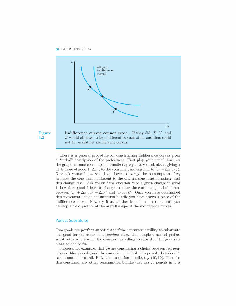
38 PREFERENCES (Ch. 3)
x
X
Y
Z
x
Allegedindifferencecurves
2
1
Figure3.2
Indifference curves cannot cross. If they did, X, Y , andZ would all have to be indifferent to each other and thus couldnot lie on distinct indifference curves.
There is a general procedure for constructing indifference curves givena “verbal” description of the preferences. First plop your pencil down onthe graph at some consumption bundle (x1, x2). Now think about giving alittle more of good 1, Δx1, to the consumer, moving him to (x1+Δx1, x2).Now ask yourself how would you have to change the consumption of x2
to make the consumer indifferent to the original consumption point? Callthis change Δx2. Ask yourself the question “For a given change in good1, how does good 2 have to change to make the consumer just indifferentbetween (x1 + Δx1, x2 + Δx2) and (x1, x2)?” Once you have determinedthis movement at one consumption bundle you have drawn a piece of theindifference curve. Now try it at another bundle, and so on, until youdevelop a clear picture of the overall shape of the indifference curves.
Perfect Substitutes
Two goods are perfect substitutes if the consumer is willing to substituteone good for the other at a constant rate. The simplest case of perfectsubstitutes occurs when the consumer is willing to substitute the goods ona one-to-one basis.Suppose, for example, that we are considering a choice between red pen-
cils and blue pencils, and the consumer involved likes pencils, but doesn’tcare about color at all. Pick a consumption bundle, say (10, 10). Then forthis consumer, any other consumption bundle that has 20 pencils in it is
EXAMPLES OF PREFERENCES 39
just as good as (10, 10). Mathematically speaking, any consumption bun-dle (x1, x2) such that x1 + x2 = 20 will be on this consumer’s indifferencecurve through (10, 10). Thus the indifference curves for this consumer areall parallel straight lines with a slope of −1, as depicted in Figure 3.3.Bundles with more total pencils are preferred to bundles with fewer totalpencils, so the direction of increasing preference is up and to the right, asillustrated in Figure 3.3.How does this work in terms of general procedure for drawing indifference
curves? If we are at (10, 10), and we increase the amount of the first goodby one unit to 11, how much do we have to change the second good to getback to the original indifference curve? The answer is clearly that we haveto decrease the second good by 1 unit. Thus the indifference curve through(10, 10) has a slope of −1. The same procedure can be carried out at anybundle of goods with the same results—in this case all the indifferencecurves have a constant slope of −1.
Indifference curves
x2
x1
Perfect substitutes. The consumer only cares about the totalnumber of pencils, not about their colors. Thus the indifferencecurves are straight lines with a slope of −1.
Figure3.3
The important fact about perfect substitutes is that the indifferencecurves have a constant slope. Suppose, for example, that we graphed bluepencils on the vertical axis and pairs of red pencils on the horizontal axis.The indifference curves for these two goods would have a slope of −2, sincethe consumer would be willing to give up two blue pencils to get one morepair of red pencils.
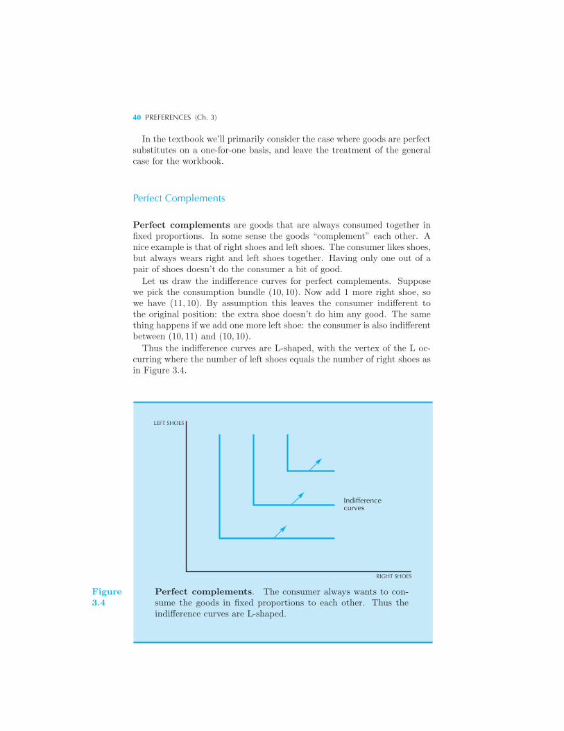
40 PREFERENCES (Ch. 3)
In the textbook we’ll primarily consider the case where goods are perfectsubstitutes on a one-for-one basis, and leave the treatment of the generalcase for the workbook.
Perfect Complements
Perfect complements are goods that are always consumed together infixed proportions. In some sense the goods “complement” each other. Anice example is that of right shoes and left shoes. The consumer likes shoes,but always wears right and left shoes together. Having only one out of apair of shoes doesn’t do the consumer a bit of good.
Let us draw the indifference curves for perfect complements. Supposewe pick the consumption bundle (10, 10). Now add 1 more right shoe, sowe have (11, 10). By assumption this leaves the consumer indifferent tothe original position: the extra shoe doesn’t do him any good. The samething happens if we add one more left shoe: the consumer is also indifferentbetween (10, 11) and (10, 10).
Thus the indifference curves are L-shaped, with the vertex of the L oc-curring where the number of left shoes equals the number of right shoes asin Figure 3.4.
LEFT SHOES
Indifferencecurves
RIGHT SHOES
Figure3.4
Perfect complements. The consumer always wants to con-sume the goods in fixed proportions to each other. Thus theindifference curves are L-shaped.
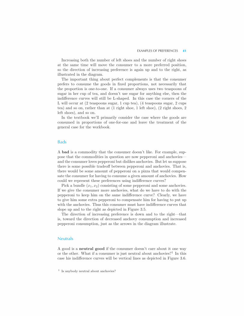
EXAMPLES OF PREFERENCES 41
Increasing both the number of left shoes and the number of right shoesat the same time will move the consumer to a more preferred position,so the direction of increasing preference is again up and to the right, asillustrated in the diagram.The important thing about perfect complements is that the consumer
prefers to consume the goods in fixed proportions, not necessarily thatthe proportion is one-to-one. If a consumer always uses two teaspoons ofsugar in her cup of tea, and doesn’t use sugar for anything else, then theindifference curves will still be L-shaped. In this case the corners of theL will occur at (2 teaspoons sugar, 1 cup tea), (4 teaspoons sugar, 2 cupstea) and so on, rather than at (1 right shoe, 1 left shoe), (2 right shoes, 2left shoes), and so on.In the textbook we’ll primarily consider the case where the goods are
consumed in proportions of one-for-one and leave the treatment of thegeneral case for the workbook.
Bads
A bad is a commodity that the consumer doesn’t like. For example, sup-pose that the commodities in question are now pepperoni and anchovies—and the consumer loves pepperoni but dislikes anchovies. But let us supposethere is some possible tradeoff between pepperoni and anchovies. That is,there would be some amount of pepperoni on a pizza that would compen-sate the consumer for having to consume a given amount of anchovies. Howcould we represent these preferences using indifference curves?Pick a bundle (x1, x2) consisting of some pepperoni and some anchovies.
If we give the consumer more anchovies, what do we have to do with thepepperoni to keep him on the same indifference curve? Clearly, we haveto give him some extra pepperoni to compensate him for having to put upwith the anchovies. Thus this consumer must have indifference curves thatslope up and to the right as depicted in Figure 3.5.The direction of increasing preference is down and to the right—that
is, toward the direction of decreased anchovy consumption and increasedpepperoni consumption, just as the arrows in the diagram illustrate.
Neutrals
A good is a neutral good if the consumer doesn’t care about it one wayor the other. What if a consumer is just neutral about anchovies?1 In thiscase his indifference curves will be vertical lines as depicted in Figure 3.6.
1 Is anybody neutral about anchovies?
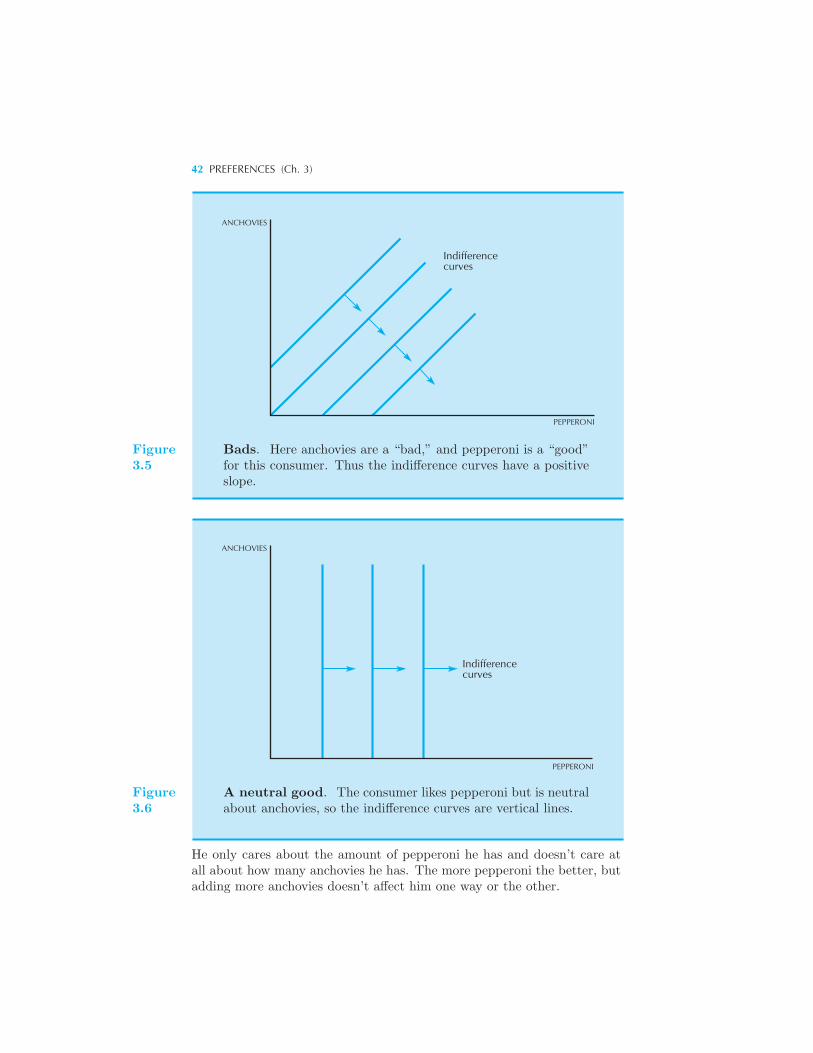
42 PREFERENCES (Ch. 3)
ANCHOVIES
Indifferencecurves
PEPPERONI
Figure3.5
Bads. Here anchovies are a “bad,” and pepperoni is a “good”for this consumer. Thus the indifference curves have a positiveslope.
ANCHOVIES
Indifferencecurves
PEPPERONI
Figure3.6
A neutral good. The consumer likes pepperoni but is neutralabout anchovies, so the indifference curves are vertical lines.
He only cares about the amount of pepperoni he has and doesn’t care atall about how many anchovies he has. The more pepperoni the better, butadding more anchovies doesn’t affect him one way or the other.
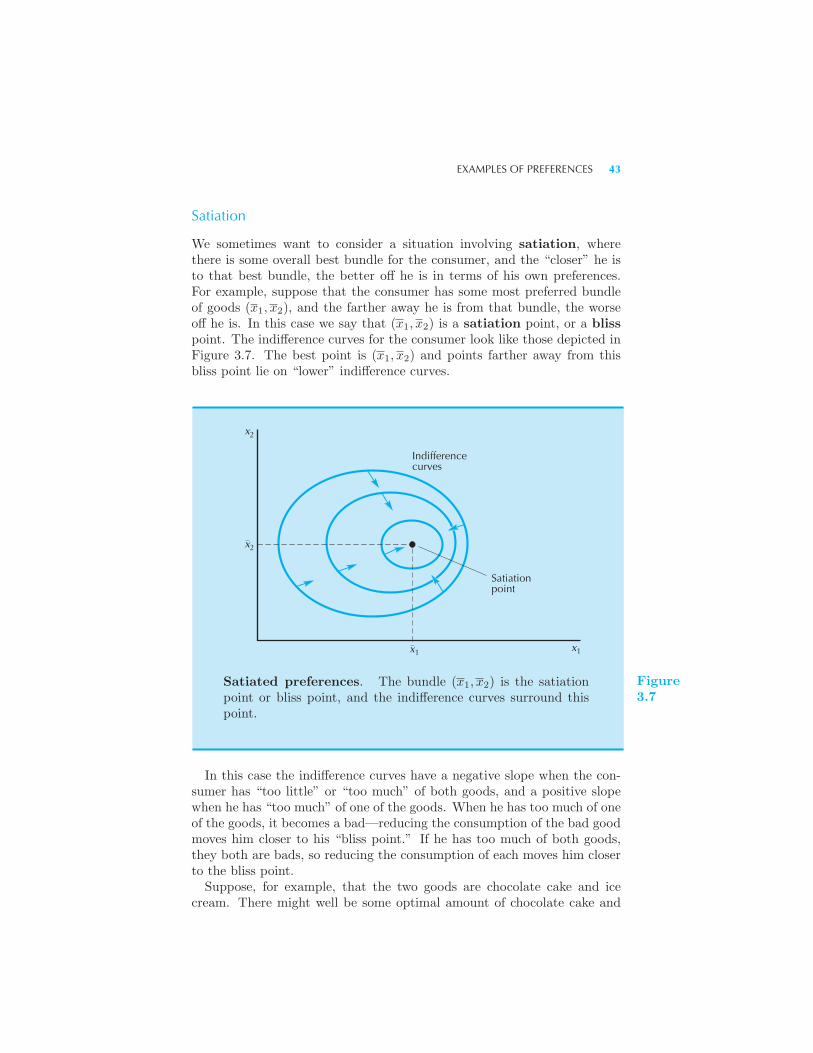
EXAMPLES OF PREFERENCES 43
Satiation
We sometimes want to consider a situation involving satiation, wherethere is some overall best bundle for the consumer, and the “closer” he isto that best bundle, the better off he is in terms of his own preferences.For example, suppose that the consumer has some most preferred bundleof goods (x1, x2), and the farther away he is from that bundle, the worseoff he is. In this case we say that (x1, x2) is a satiation point, or a blisspoint. The indifference curves for the consumer look like those depicted inFigure 3.7. The best point is (x1, x2) and points farther away from thisbliss point lie on “lower” indifference curves.
Indifferencecurves
Satiationpoint
x2
2x
x1 1x
Satiated preferences. The bundle (x1, x2) is the satiationpoint or bliss point, and the indifference curves surround thispoint.
Figure3.7
In this case the indifference curves have a negative slope when the con-sumer has “too little” or “too much” of both goods, and a positive slopewhen he has “too much” of one of the goods. When he has too much of oneof the goods, it becomes a bad—reducing the consumption of the bad goodmoves him closer to his “bliss point.” If he has too much of both goods,they both are bads, so reducing the consumption of each moves him closerto the bliss point.Suppose, for example, that the two goods are chocolate cake and ice
cream. There might well be some optimal amount of chocolate cake and
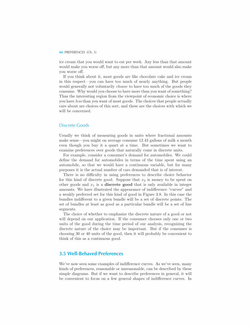
44 PREFERENCES (Ch. 3)
ice cream that you would want to eat per week. Any less than that amountwould make you worse off, but any more than that amount would also makeyou worse off.If you think about it, most goods are like chocolate cake and ice cream
in this respect—you can have too much of nearly anything. But peoplewould generally not voluntarily choose to have too much of the goods theyconsume. Why would you choose to have more than you want of something?Thus the interesting region from the viewpoint of economic choice is whereyou have less than you want of most goods. The choices that people actuallycare about are choices of this sort, and these are the choices with which wewill be concerned.
Discrete Goods
Usually we think of measuring goods in units where fractional amountsmake sense—you might on average consume 12.43 gallons of milk a montheven though you buy it a quart at a time. But sometimes we want toexamine preferences over goods that naturally come in discrete units.For example, consider a consumer’s demand for automobiles. We could
define the demand for automobiles in terms of the time spent using anautomobile, so that we would have a continuous variable, but for manypurposes it is the actual number of cars demanded that is of interest.There is no difficulty in using preferences to describe choice behavior
for this kind of discrete good. Suppose that x2 is money to be spent onother goods and x1 is a discrete good that is only available in integeramounts. We have illustrated the appearance of indifference “curves” anda weakly preferred set for this kind of good in Figure 3.8. In this case thebundles indifferent to a given bundle will be a set of discrete points. Theset of bundles at least as good as a particular bundle will be a set of linesegments.The choice of whether to emphasize the discrete nature of a good or not
will depend on our application. If the consumer chooses only one or twounits of the good during the time period of our analysis, recognizing thediscrete nature of the choice may be important. But if the consumer ischoosing 30 or 40 units of the good, then it will probably be convenient tothink of this as a continuous good.
3.5 Well-Behaved Preferences
We’ve now seen some examples of indifference curves. As we’ve seen, manykinds of preferences, reasonable or unreasonable, can be described by thesesimple diagrams. But if we want to describe preferences in general, it willbe convenient to focus on a few general shapes of indifference curves. In
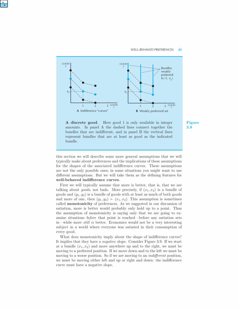
WELL-BEHAVED PREFERENCES 45
GOOD2
GOOD1
x2
Bundlesweaklypreferredto (1, x )
2
B Weakly preferrred set
1 2 3
GOOD2
GOOD1
x2
A Indifference "curves"
1 2 3
A discrete good. Here good 1 is only available in integeramounts. In panel A the dashed lines connect together thebundles that are indifferent, and in panel B the vertical linesrepresent bundles that are at least as good as the indicatedbundle.
Figure3.8
this section we will describe some more general assumptions that we willtypically make about preferences and the implications of these assumptionsfor the shapes of the associated indifference curves. These assumptionsare not the only possible ones; in some situations you might want to usedifferent assumptions. But we will take them as the defining features forwell-behaved indifference curves.
First we will typically assume that more is better, that is, that we aretalking about goods, not bads. More precisely, if (x1, x2) is a bundle ofgoods and (y1, y2) is a bundle of goods with at least as much of both goodsand more of one, then (y1, y2) � (x1, x2). This assumption is sometimescalled monotonicity of preferences. As we suggested in our discussion ofsatiation, more is better would probably only hold up to a point. Thusthe assumption of monotonicity is saying only that we are going to ex-amine situations before that point is reached—before any satiation setsin—while more still is better. Economics would not be a very interestingsubject in a world where everyone was satiated in their consumption ofevery good.
What does monotonicity imply about the shape of indifference curves?It implies that they have a negative slope. Consider Figure 3.9. If we startat a bundle (x1, x2) and move anywhere up and to the right, we must bemoving to a preferred position. If we move down and to the left we must bemoving to a worse position. So if we are moving to an indifferent position,we must be moving either left and up or right and down: the indifferencecurve must have a negative slope.
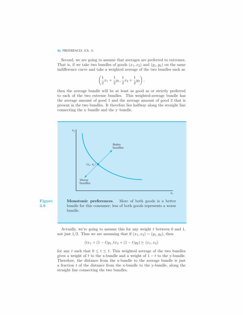
46 PREFERENCES (Ch. 3)
Second, we are going to assume that averages are preferred to extremes.That is, if we take two bundles of goods (x1, x2) and (y1, y2) on the sameindifference curve and take a weighted average of the two bundles such as
(1
2x1 +
1
2y1,
1
2x2 +
1
2y2
),
then the average bundle will be at least as good as or strictly preferredto each of the two extreme bundles. This weighted-average bundle hasthe average amount of good 1 and the average amount of good 2 that ispresent in the two bundles. It therefore lies halfway along the straight lineconnecting the x–bundle and the y–bundle.
x2
(x , x )1 2
1x
Worsebundles
Betterbundles
Figure3.9
Monotonic preferences. More of both goods is a betterbundle for this consumer; less of both goods represents a worsebundle.
Actually, we’re going to assume this for any weight t between 0 and 1,not just 1/2. Thus we are assuming that if (x1, x2) ∼ (y1, y2), then
(tx1 + (1− t)y1, tx2 + (1− t)y2) � (x1, x2)
for any t such that 0 ≤ t ≤ 1. This weighted average of the two bundlesgives a weight of t to the x-bundle and a weight of 1 − t to the y-bundle.Therefore, the distance from the x-bundle to the average bundle is justa fraction t of the distance from the x-bundle to the y-bundle, along thestraight line connecting the two bundles.
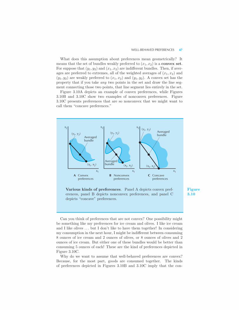
WELL-BEHAVED PREFERENCES 47
What does this assumption about preferences mean geometrically? Itmeans that the set of bundles weakly preferred to (x1, x2) is a convex set.For suppose that (y1, y2) and (x1, x2) are indifferent bundles. Then, if aver-ages are preferred to extremes, all of the weighted averages of (x1, x2) and(y1, y2) are weakly preferred to (x1, x2) and (y1, y2). A convex set has theproperty that if you take any two points in the set and draw the line seg-ment connecting those two points, that line segment lies entirely in the set.Figure 3.10A depicts an example of convex preferences, while Figures
3.10B and 3.10C show two examples of nonconvex preferences. Figure3.10C presents preferences that are so nonconvex that we might want tocall them “concave preferences.”
x2x2x2
(y , y )21
(x , x )1 2
1x
(x , x )1 2 (x , x )1 2
1x 1x
C Concave preferences
B Nonconvex preferences
A Convex preferences
(y , y )21
(y , y )21 Averagedbundle
Averagedbundle
Averagedbundle
Various kinds of preferences. Panel A depicts convex pref-erences, panel B depicts nonconvex preferences, and panel Cdepicts “concave” preferences.
Figure3.10
Can you think of preferences that are not convex? One possibility mightbe something like my preferences for ice cream and olives. I like ice creamand I like olives . . . but I don’t like to have them together! In consideringmy consumption in the next hour, I might be indifferent between consuming8 ounces of ice cream and 2 ounces of olives, or 8 ounces of olives and 2ounces of ice cream. But either one of these bundles would be better thanconsuming 5 ounces of each! These are the kind of preferences depicted inFigure 3.10C.Why do we want to assume that well-behaved preferences are convex?
Because, for the most part, goods are consumed together. The kindsof preferences depicted in Figures 3.10B and 3.10C imply that the con-
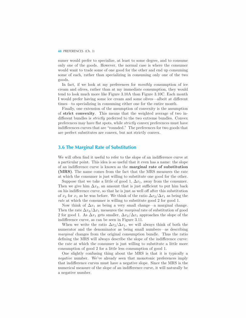
48 PREFERENCES (Ch. 3)
sumer would prefer to specialize, at least to some degree, and to consumeonly one of the goods. However, the normal case is where the consumerwould want to trade some of one good for the other and end up consumingsome of each, rather than specializing in consuming only one of the twogoods.In fact, if we look at my preferences for monthly consumption of ice
cream and olives, rather than at my immediate consumption, they wouldtend to look much more like Figure 3.10A than Figure 3.10C. Each monthI would prefer having some ice cream and some olives—albeit at differenttimes—to specializing in consuming either one for the entire month.Finally, one extension of the assumption of convexity is the assumption
of strict convexity. This means that the weighted average of two in-different bundles is strictly preferred to the two extreme bundles. Convexpreferences may have flat spots, while strictly convex preferences must haveindifferences curves that are “rounded.” The preferences for two goods thatare perfect substitutes are convex, but not strictly convex.
3.6 The Marginal Rate of Substitution
We will often find it useful to refer to the slope of an indifference curve ata particular point. This idea is so useful that it even has a name: the slopeof an indifference curve is known as the marginal rate of substitution(MRS). The name comes from the fact that the MRS measures the rateat which the consumer is just willing to substitute one good for the other.Suppose that we take a little of good 1, Δx1, away from the consumer.
Then we give him Δx2, an amount that is just sufficient to put him backon his indifference curve, so that he is just as well off after this substitutionof x2 for x1 as he was before. We think of the ratio Δx2/Δx1 as being therate at which the consumer is willing to substitute good 2 for good 1.Now think of Δx1 as being a very small change—a marginal change.
Then the rate Δx2/Δx1 measures the marginal rate of substitution of good2 for good 1. As Δx1 gets smaller, Δx2/Δx1 approaches the slope of theindifference curve, as can be seen in Figure 3.11.When we write the ratio Δx2/Δx1, we will always think of both the
numerator and the denominator as being small numbers—as describingmarginal changes from the original consumption bundle. Thus the ratiodefining the MRS will always describe the slope of the indifference curve:the rate at which the consumer is just willing to substitute a little moreconsumption of good 2 for a little less consumption of good 1.One slightly confusing thing about the MRS is that it is typically a
negative number. We’ve already seen that monotonic preferences implythat indifference curves must have a negative slope. Since the MRS is thenumerical measure of the slope of an indifference curve, it will naturally bea negative number.
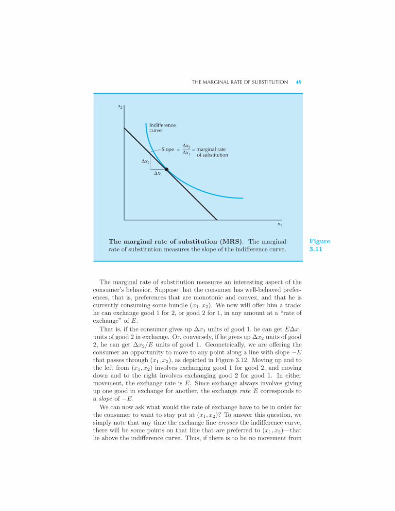
THE MARGINAL RATE OF SUBSTITUTION 49
Indifferencecurve
x
Δx
Δx
2
2
1
1
Slope = = marginal rate of substitution
x
2
1ΔxΔx
The marginal rate of substitution (MRS). The marginalrate of substitution measures the slope of the indifference curve.
Figure3.11
The marginal rate of substitution measures an interesting aspect of theconsumer’s behavior. Suppose that the consumer has well-behaved prefer-ences, that is, preferences that are monotonic and convex, and that he iscurrently consuming some bundle (x1, x2). We now will offer him a trade:he can exchange good 1 for 2, or good 2 for 1, in any amount at a “rate ofexchange” of E.
That is, if the consumer gives up Δx1 units of good 1, he can get EΔx1
units of good 2 in exchange. Or, conversely, if he gives up Δx2 units of good2, he can get Δx2/E units of good 1. Geometrically, we are offering theconsumer an opportunity to move to any point along a line with slope −Ethat passes through (x1, x2), as depicted in Figure 3.12. Moving up and tothe left from (x1, x2) involves exchanging good 1 for good 2, and movingdown and to the right involves exchanging good 2 for good 1. In eithermovement, the exchange rate is E. Since exchange always involves givingup one good in exchange for another, the exchange rate E corresponds toa slope of −E.
We can now ask what would the rate of exchange have to be in order forthe consumer to want to stay put at (x1, x2)? To answer this question, wesimply note that any time the exchange line crosses the indifference curve,there will be some points on that line that are preferred to (x1, x2)—thatlie above the indifference curve. Thus, if there is to be no movement from
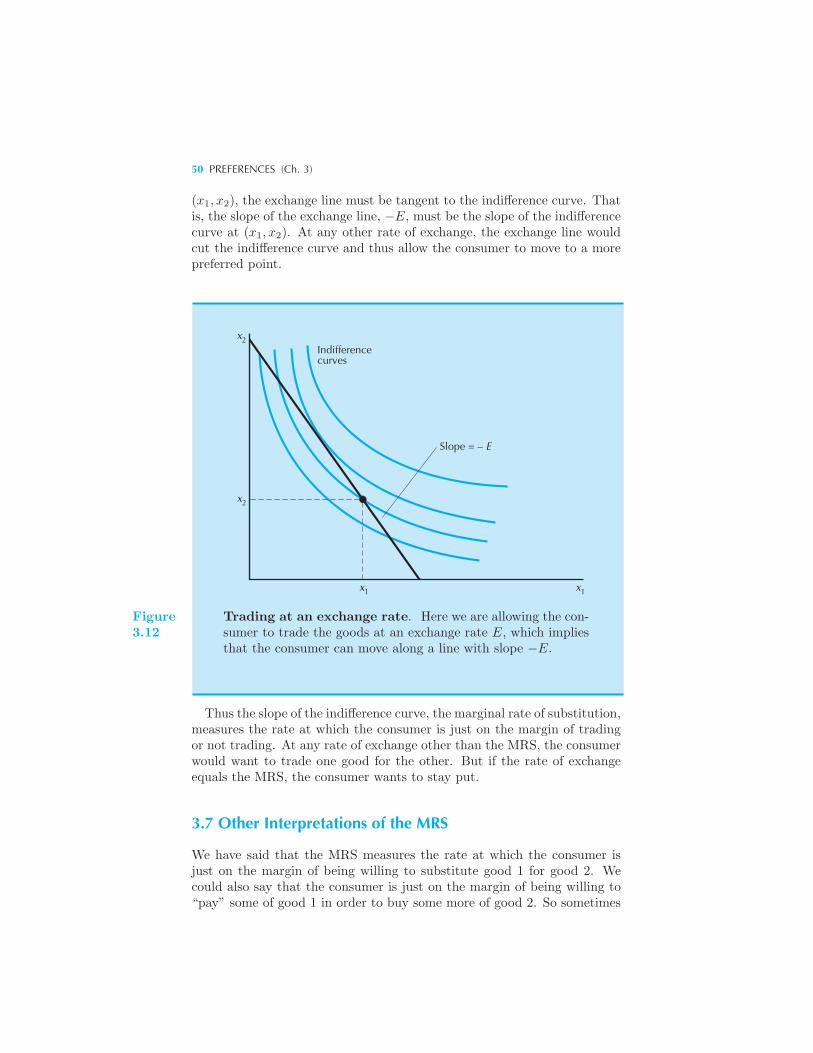
50 PREFERENCES (Ch. 3)
(x1, x2), the exchange line must be tangent to the indifference curve. Thatis, the slope of the exchange line, −E, must be the slope of the indifferencecurve at (x1, x2). At any other rate of exchange, the exchange line wouldcut the indifference curve and thus allow the consumer to move to a morepreferred point.
x2
x2
1x 1x
Indifferencecurves
Slope = – E
Figure3.12
Trading at an exchange rate. Here we are allowing the con-sumer to trade the goods at an exchange rate E, which impliesthat the consumer can move along a line with slope −E.
Thus the slope of the indifference curve, the marginal rate of substitution,measures the rate at which the consumer is just on the margin of tradingor not trading. At any rate of exchange other than the MRS, the consumerwould want to trade one good for the other. But if the rate of exchangeequals the MRS, the consumer wants to stay put.
3.7 Other Interpretations of the MRS
We have said that the MRS measures the rate at which the consumer isjust on the margin of being willing to substitute good 1 for good 2. Wecould also say that the consumer is just on the margin of being willing to“pay” some of good 1 in order to buy some more of good 2. So sometimes
BEHAVIOR OF THE MRS 51
you hear people say that the slope of the indifference curve measures themarginal willingness to pay.If good 2 represents the consumption of “all other goods,” and it is
measured in dollars that you can spend on other goods, then the marginal-willingness-to-pay interpretation is very natural. The marginal rate of sub-stitution of good 2 for good 1 is how many dollars you would just be willingto give up spending on other goods in order to consume a little bit moreof good 1. Thus the MRS measures the marginal willingness to give updollars in order to consume a small amount more of good 1. But giving upthose dollars is just like paying dollars in order to consume a little more ofgood 1.If you use the marginal-willingness-to-pay interpretation of the MRS, you
should be careful to emphasize both the “marginal” and the “willingness”aspects. The MRS measures the amount of good 2 that one is willing topay for a marginal amount of extra consumption of good 1. How muchyou actually have to pay for some given amount of extra consumption maybe different than the amount you are willing to pay. How much you haveto pay will depend on the price of the good in question. How much youare willing to pay doesn’t depend on the price—it is determined by yourpreferences.Similarly, how much you may be willing to pay for a large change in
consumption may be different from how much you are willing to pay fora marginal change. How much you actually end up buying of a good willdepend on your preferences for that good and the prices that you face. Howmuch you would be willing to pay for a small amount extra of the good isa feature only of your preferences.
3.8 Behavior of the MRS
It is sometimes useful to describe the shapes of indifference curves by de-scribing the behavior of the marginal rate of substitution. For example,the “perfect substitutes” indifference curves are characterized by the factthat the MRS is constant at −1. The “neutrals” case is characterized bythe fact that the MRS is everywhere infinite. The preferences for “perfectcomplements” are characterized by the fact that the MRS is either zero orinfinity, and nothing in between.We’ve already pointed out that the assumption of monotonicity implies
that indifference curves must have a negative slope, so the MRS alwaysinvolves reducing the consumption of one good in order to get more ofanother for monotonic preferences.The case of convex indifference curves exhibits yet another kind of be-
havior for the MRS. For strictly convex indifference curves, the MRS—theslope of the indifference curve—decreases (in absolute value) as we increasex1. Thus the indifference curves exhibit a diminishing marginal rate of
52 PREFERENCES (Ch. 3)
substitution. This means that the amount of good 1 that the person iswilling to give up for an additional amount of good 2 increases the amountof good 1 increases. Stated in this way, convexity of indifference curvesseems very natural: it says that the more you have of one good, the morewilling you are to give some of it up in exchange for the other good. (Butremember the ice cream and olives example—for some pairs of goods thisassumption might not hold!)
Summary
1. Economists assume that a consumer can rank various consumption pos-sibilities. The way in which the consumer ranks the consumption bundlesdescribes the consumer’s preferences.
2. Indifference curves can be used to depict different kinds of preferences.
3. Well-behaved preferences are monotonic (meaning more is better) andconvex (meaning averages are preferred to extremes).
4. The marginal rate of substitution (MRS) measures the slope of the in-difference curve. This can be interpreted as how much the consumer iswilling to give up of good 2 to acquire more of good 1.
REVIEW QUESTIONS
1. If we observe a consumer choosing (x1, x2) when (y1, y2) is available onetime, are we justified in concluding that (x1, x2) � (y1, y2)?
2. Consider a group of people A, B, C and the relation “at least as tall as,”as in “A is at least as tall as B.” Is this relation transitive? Is it complete?
3. Take the same group of people and consider the relation “strictly tallerthan.” Is this relation transitive? Is it reflexive? Is it complete?
4. A college football coach says that given any two linemen A and B, healways prefers the one who is bigger and faster. Is this preference relationtransitive? Is it complete?
5. Can an indifference curve cross itself? For example, could Figure 3.2depict a single indifference curve?
6. Could Figure 3.2 be a single indifference curve if preferences are mono-tonic?
REVIEW QUESTIONS 53
7. If both pepperoni and anchovies are bads, will the indifference curvehave a positive or a negative slope?
8. Explain why convex preferences means that “averages are preferred toextremes.”
9. What is your marginal rate of substitution of $1 bills for $5 bills?
10. If good 1 is a “neutral,” what is its marginal rate of substitution forgood 2?
11. Think of some other goods for which your preferences might be concave.

CHAPTER 4
UTILITY
In Victorian days, philosophers and economists talked blithely of “utility”as an indicator of a person’s overall well-being. Utility was thought of asa numeric measure of a person’s happiness. Given this idea, it was naturalto think of consumers making choices so as to maximize their utility, thatis, to make themselves as happy as possible.The trouble is that these classical economists never really described how
we were to measure utility. How are we supposed to quantify the “amount”of utility associated with different choices? Is one person’s utility the sameas another’s? What would it mean to say that an extra candy bar wouldgive me twice as much utility as an extra carrot? Does the concept of utilityhave any independent meaning other than its being what people maximize?Because of these conceptual problems, economists have abandoned the
old-fashioned view of utility as being a measure of happiness. Instead,the theory of consumer behavior has been reformulated entirely in termsof consumer preferences, and utility is seen only as a way to describepreferences.Economists gradually came to recognize that all that mattered about
utility as far as choice behavior was concerned was whether one bundlehad a higher utility than another—how much higher didn’t really matter.
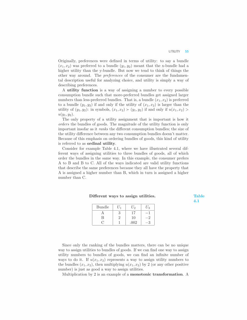
UTILITY 55
Originally, preferences were defined in terms of utility: to say a bundle(x1, x2) was preferred to a bundle (y1, y2) meant that the x-bundle had ahigher utility than the y-bundle. But now we tend to think of things theother way around. The preferences of the consumer are the fundamen-tal description useful for analyzing choice, and utility is simply a way ofdescribing preferences.
A utility function is a way of assigning a number to every possibleconsumption bundle such that more-preferred bundles get assigned largernumbers than less-preferred bundles. That is, a bundle (x1, x2) is preferredto a bundle (y1, y2) if and only if the utility of (x1, x2) is larger than theutility of (y1, y2): in symbols, (x1, x2) � (y1, y2) if and only if u(x1, x2) >u(y1, y2).
The only property of a utility assignment that is important is how itorders the bundles of goods. The magnitude of the utility function is onlyimportant insofar as it ranks the different consumption bundles; the size ofthe utility difference between any two consumption bundles doesn’t matter.Because of this emphasis on ordering bundles of goods, this kind of utilityis referred to as ordinal utility.
Consider for example Table 4.1, where we have illustrated several dif-ferent ways of assigning utilities to three bundles of goods, all of whichorder the bundles in the same way. In this example, the consumer prefersA to B and B to C. All of the ways indicated are valid utility functionsthat describe the same preferences because they all have the property thatA is assigned a higher number than B, which in turn is assigned a highernumber than C.
Different ways to assign utilities.
Bundle U1 U2 U3
A 3 17 −1B 2 10 −2C 1 .002 −3
Table4.1
Since only the ranking of the bundles matters, there can be no uniqueway to assign utilities to bundles of goods. If we can find one way to assignutility numbers to bundles of goods, we can find an infinite number ofways to do it. If u(x1, x2) represents a way to assign utility numbers tothe bundles (x1, x2), then multiplying u(x1, x2) by 2 (or any other positivenumber) is just as good a way to assign utilities.
Multiplication by 2 is an example of a monotonic transformation. A
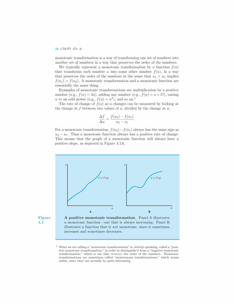
56 UTILITY (Ch. 4)
monotonic transformation is a way of transforming one set of numbers intoanother set of numbers in a way that preserves the order of the numbers.We typically represent a monotonic transformation by a function f(u)
that transforms each number u into some other number f(u), in a waythat preserves the order of the numbers in the sense that u1 > u2 impliesf(u1) > f(u2). A monotonic transformation and a monotonic function areessentially the same thing.Examples of monotonic transformations are multiplication by a positive
number (e.g., f(u) = 3u), adding any number (e.g., f(u) = u+17), raisingu to an odd power (e.g., f(u) = u3), and so on.1
The rate of change of f(u) as u changes can be measured by looking atthe change in f between two values of u, divided by the change in u:
Δf
Δu=
f(u2)− f(u1)
u2 − u1.
For a monotonic transformation, f(u2)−f(u1) always has the same sign asu2 − u1. Thus a monotonic function always has a positive rate of change.This means that the graph of a monotonic function will always have apositive slope, as depicted in Figure 4.1A.
vv
v = f (u )
uuA B
v = f (u )
Figure4.1
A positive monotonic transformation. Panel A illustratesa monotonic function—one that is always increasing. Panel Billustrates a function that is not monotonic, since it sometimesincreases and sometimes decreases.
1 What we are calling a “monotonic transformation” is, strictly speaking, called a “posi-tive monotonic transformation,” in order to distinguish it from a “negative monotonictransformation,” which is one that reverses the order of the numbers. Monotonictransformations are sometimes called “monotonous transformations,” which seemsunfair, since they can actually be quite interesting.
CARDINAL UTILITY 57
If f(u) is any monotonic transformation of a utility function that repre-sents some particular preferences, then f(u(x1, x2)) is also a utility functionthat represents those same preferences.Why? The argument is given in the following three statements:
1. To say that u(x1, x2) represents some particular preferences means thatu(x1, x2) > u(y1, y2) if and only if (x1, x2) � (y1, y2).
2. But if f(u) is a monotonic transformation, then u(x1, x2) > u(y1, y2) ifand only if f(u(x1, x2)) > f(u(y1, y2)).
3. Therefore, f(u(x1, x2)) > f(u(y1, y2)) if and only if (x1, x2) � (y1, y2),so the function f(u) represents the preferences in the same way as theoriginal utility function u(x1, x2).
We summarize this discussion by stating the following principle: a mono-tonic transformation of a utility function is a utility function that representsthe same preferences as the original utility function.Geometrically, a utility function is a way to label indifference curves.
Since every bundle on an indifference curve must have the same utility, autility function is a way of assigning numbers to the different indifferencecurves in a way that higher indifference curves get assigned larger num-bers. Seen from this point of view a monotonic transformation is just arelabeling of indifference curves. As long as indifference curves containingmore-preferred bundles get a larger label than indifference curves contain-ing less-preferred bundles, the labeling will represent the same preferences.
4.1 Cardinal Utility
There are some theories of utility that attach a significance to the magni-tude of utility. These are known as cardinal utility theories. In a theoryof cardinal utility, the size of the utility difference between two bundles ofgoods is supposed to have some sort of significance.We know how to tell whether a given person prefers one bundle of goods
to another: we simply offer him or her a choice between the two bundlesand see which one is chosen. Thus we know how to assign an ordinal utilityto the two bundles of goods: we just assign a higher utility to the chosenbundle than to the rejected bundle. Any assignment that does this will bea utility function. Thus we have an operational criterion for determiningwhether one bundle has a higher utility than another bundle for someindividual.But how do we tell if a person likes one bundle twice as much as another?
How could you even tell if you like one bundle twice as much as another?One could propose various definitions for this kind of assignment: I like
one bundle twice as much as another if I am willing to pay twice as muchfor it. Or, I like one bundle twice as much as another if I am willing to run
58 UTILITY (Ch. 4)
twice as far to get it, or to wait twice as long, or to gamble for it at twicethe odds.
There is nothing wrong with any of these definitions; each one wouldgive rise to a way of assigning utility levels in which the magnitude of thenumbers assigned had some operational significance. But there isn’t muchright about them either. Although each of them is a possible interpretationof what it means to want one thing twice as much as another, none of themappears to be an especially compelling interpretation of that statement.
Even if we did find a way of assigning utility magnitudes that seemedto be especially compelling, what good would it do us in describing choicebehavior? To tell whether one bundle or another will be chosen, we onlyhave to know which is preferred—which has the larger utility. Knowinghow much larger doesn’t add anything to our description of choice. Sincecardinal utility isn’t needed to describe choice behavior and there is nocompelling way to assign cardinal utilities anyway, we will stick with apurely ordinal utility framework.
4.2 Constructing a Utility Function
But are we assured that there is any way to assign ordinal utilities? Givena preference ordering can we always find a utility function that will orderbundles of goods in the same way as those preferences? Is there a utilityfunction that describes any reasonable preference ordering?
Not all kinds of preferences can be represented by a utility function.For example, suppose that someone had intransitive preferences so thatA � B � C � A. Then a utility function for these preferences would haveto consist of numbers u(A), u(B), and u(C) such that u(A) > u(B) >u(C) > u(A). But this is impossible.
However, if we rule out perverse cases like intransitive preferences, itturns out that we will typically be able to find a utility function to representpreferences. We will illustrate one construction here, and another one inChapter 14.
Suppose that we are given an indifference map as in Figure 4.2. We knowthat a utility function is a way to label the indifference curves such thathigher indifference curves get larger numbers. How can we do this?
One easy way is to draw the diagonal line illustrated and label eachindifference curve with its distance from the origin measured along theline.
How do we know that this is a utility function? It is not hard to see thatif preferences are monotonic then the line through the origin must intersectevery indifference curve exactly once. Thus every bundle is getting a label,and those bundles on higher indifference curves are getting larger labels—and that’s all it takes to be a utility function.
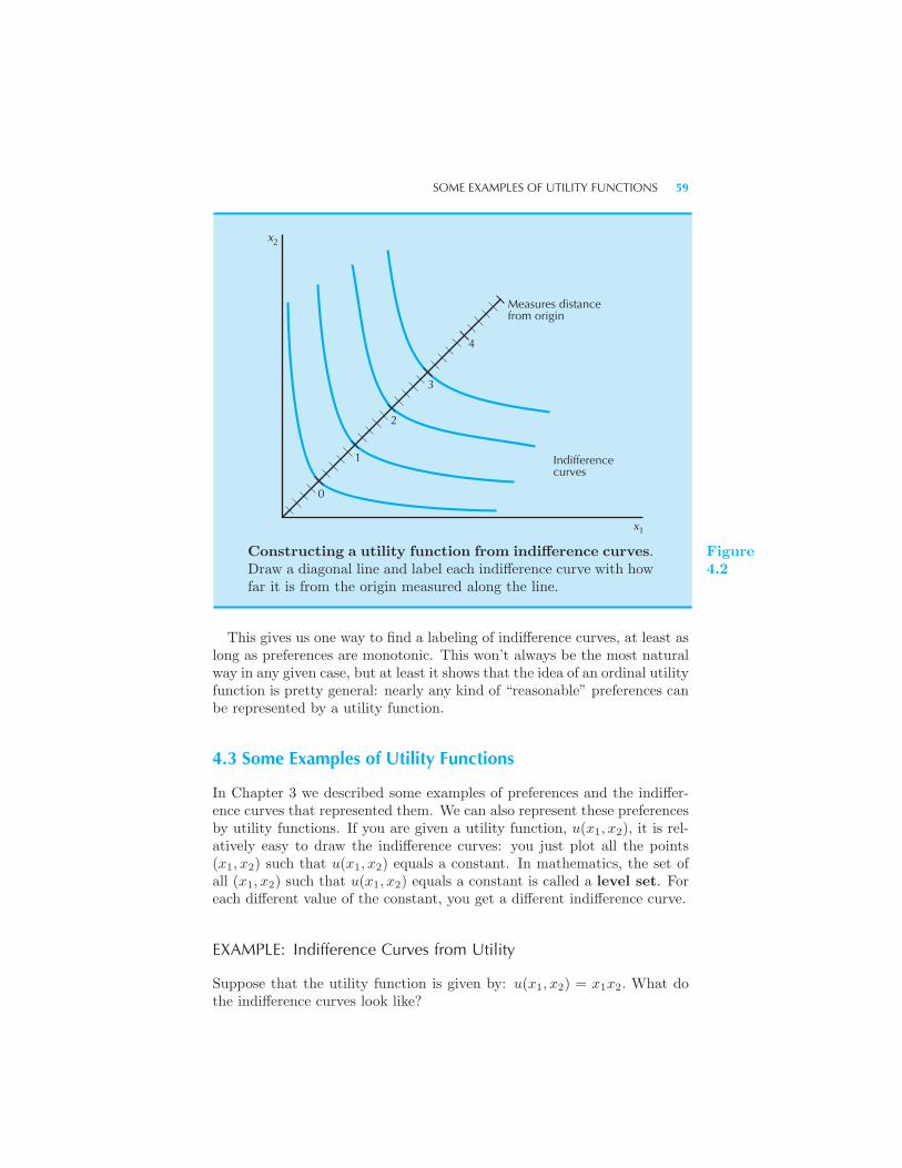
SOME EXAMPLES OF UTILITY FUNCTIONS 59
x
x
2
1
4
3
2
1
0
Measures distancefrom origin
Indifferencecurves
Constructing a utility function from indifference curves.Draw a diagonal line and label each indifference curve with howfar it is from the origin measured along the line.
Figure4.2
This gives us one way to find a labeling of indifference curves, at least aslong as preferences are monotonic. This won’t always be the most naturalway in any given case, but at least it shows that the idea of an ordinal utilityfunction is pretty general: nearly any kind of “reasonable” preferences canbe represented by a utility function.
4.3 Some Examples of Utility Functions
In Chapter 3 we described some examples of preferences and the indiffer-ence curves that represented them. We can also represent these preferencesby utility functions. If you are given a utility function, u(x1, x2), it is rel-atively easy to draw the indifference curves: you just plot all the points(x1, x2) such that u(x1, x2) equals a constant. In mathematics, the set ofall (x1, x2) such that u(x1, x2) equals a constant is called a level set. Foreach different value of the constant, you get a different indifference curve.
EXAMPLE: Indifference Curves from Utility
Suppose that the utility function is given by: u(x1, x2) = x1x2. What dothe indifference curves look like?
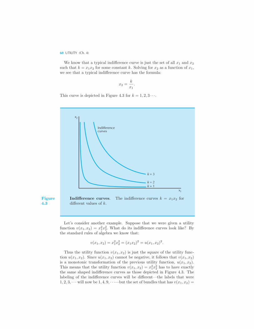
60 UTILITY (Ch. 4)
We know that a typical indifference curve is just the set of all x1 and x2
such that k = x1x2 for some constant k. Solving for x2 as a function of x1,we see that a typical indifference curve has the formula:
x2 =k
x1.
This curve is depicted in Figure 4.3 for k = 1, 2, 3 · · ·.
Indifference curves
x2
k = 3
k = 2k = 1
x1
Figure4.3
Indifference curves. The indifference curves k = x1x2 fordifferent values of k.
Let’s consider another example. Suppose that we were given a utilityfunction v(x1, x2) = x2
1x22. What do its indifference curves look like? By
the standard rules of algebra we know that:
v(x1, x2) = x21x
22 = (x1x2)
2 = u(x1, x2)2.
Thus the utility function v(x1, x2) is just the square of the utility func-tion u(x1, x2). Since u(x1, x2) cannot be negative, it follows that v(x1, x2)is a monotonic transformation of the previous utility function, u(x1, x2).This means that the utility function v(x1, x2) = x2
1x22 has to have exactly
the same shaped indifference curves as those depicted in Figure 4.3. Thelabeling of the indifference curves will be different—the labels that were1, 2, 3, · · · will now be 1, 4, 9, · · ·—but the set of bundles that has v(x1, x2) =
SOME EXAMPLES OF UTILITY FUNCTIONS 61
9 is exactly the same as the set of bundles that has u(x1, x2) = 3. Thusv(x1, x2) describes exactly the same preferences as u(x1, x2) since it ordersall of the bundles in the same way.
Going the other direction—finding a utility function that represents someindifference curves—is somewhat more difficult. There are two ways toproceed. The first way is mathematical. Given the indifference curves, wewant to find a function that is constant along each indifference curve andthat assigns higher values to higher indifference curves.
The second way is a bit more intuitive. Given a description of the pref-erences, we try to think about what the consumer is trying to maximize—what combination of the goods describes the choice behavior of the con-sumer. This may seem a little vague at the moment, but it will be moremeaningful after we discuss a few examples.
Perfect Substitutes
Remember the red pencil and blue pencil example? All that mattered tothe consumer was the total number of pencils. Thus it is natural to measureutility by the total number of pencils. Therefore we provisionally pick theutility function u(x1, x2) = x1+x2. Does this work? Just ask two things: isthis utility function constant along the indifference curves? Does it assigna higher label to more-preferred bundles? The answer to both questions isyes, so we have a utility function.
Of course, this isn’t the only utility function that we could use. We couldalso use the square of the number of pencils. Thus the utility functionv(x1, x2) = (x1 + x2)
2 = x21 + 2x1x2 + x2
2 will also represent the perfect-substitutes preferences, as would any other monotonic transformation ofu(x1, x2).
What if the consumer is willing to substitute good 1 for good 2 at a ratethat is different from one-to-one? Suppose, for example, that the consumerwould require two units of good 2 to compensate him for giving up one unitof good 1. This means that good 1 is twice as valuable to the consumer asgood 2. The utility function therefore takes the form u(x1, x2) = 2x1 + x2.Note that this utility yields indifference curves with a slope of −2.
In general, preferences for perfect substitutes can be represented by autility function of the form
u(x1, x2) = ax1 + bx2.
Here a and b are some positive numbers that measure the “value” of goods1 and 2 to the consumer. Note that the slope of a typical indifference curveis given by −a/b.

62 UTILITY (Ch. 4)
Perfect Complements
This is the left shoe–right shoe case. In these preferences the consumer onlycares about the number of pairs of shoes he has, so it is natural to choosethe number of pairs of shoes as the utility function. The number of completepairs of shoes that you have is the minimum of the number of right shoesyou have, x1, and the number of left shoes you have, x2. Thus the utilityfunction for perfect complements takes the form u(x1, x2) = min{x1, x2}.
To verify that this utility function actually works, pick a bundle of goodssuch as (10, 10). If we add one more unit of good 1 we get (11, 10),which should leave us on the same indifference curve. Does it? Yes, sincemin{10, 10} = min{11, 10} = 10.So u(x1, x2) = min{x1, x2} is a possible utility function to describe per-
fect complements. As usual, any monotonic transformation would be suit-able as well.What about the case where the consumer wants to consume the goods
in some proportion other than one-to-one? For example, what about theconsumer who always uses 2 teaspoons of sugar with each cup of tea? If x1
is the number of cups of tea available and x2 is the number of teaspoonsof sugar available, then the number of correctly sweetened cups of tea willbe min{x1,
12x2}.
This is a little tricky so we should stop to think about it. If the numberof cups of tea is greater than half the number of teaspoons of sugar, thenwe know that we won’t be able to put 2 teaspoons of sugar in each cup.In this case, we will only end up with 1
2x2 correctly sweetened cups of tea.(Substitute some numbers in for x1 and x2 to convince yourself.)Of course, any monotonic transformation of this utility function will
describe the same preferences. For example, we might want to multiply by2 to get rid of the fraction. This gives us the utility function u(x1, x2) =min{2x1, x2}.In general, a utility function that describes perfect-complement prefer-
ences is given by
u(x1, x2) = min{ax1, bx2},
where a and b are positive numbers that indicate the proportions in whichthe goods are consumed.
Quasilinear Preferences
Here’s a shape of indifference curves that we haven’t seen before. Supposethat a consumer has indifference curves that are vertical translates of oneanother, as in Figure 4.4. This means that all of the indifference curves arejust vertically “shifted” versions of one indifference curve. It follows that
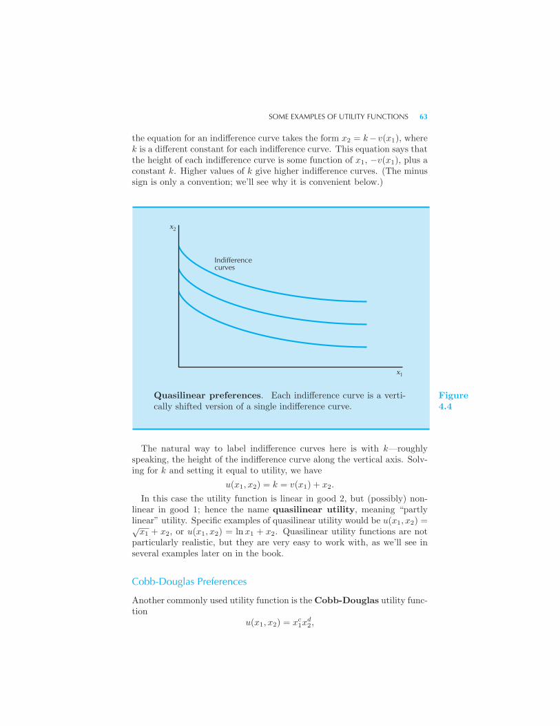
SOME EXAMPLES OF UTILITY FUNCTIONS 63
the equation for an indifference curve takes the form x2 = k−v(x1), wherek is a different constant for each indifference curve. This equation says thatthe height of each indifference curve is some function of x1, −v(x1), plus aconstant k. Higher values of k give higher indifference curves. (The minussign is only a convention; we’ll see why it is convenient below.)
x2
x1
Indifferencecurves
Quasilinear preferences. Each indifference curve is a verti-cally shifted version of a single indifference curve.
Figure4.4
The natural way to label indifference curves here is with k—roughlyspeaking, the height of the indifference curve along the vertical axis. Solv-ing for k and setting it equal to utility, we have
u(x1, x2) = k = v(x1) + x2.
In this case the utility function is linear in good 2, but (possibly) non-linear in good 1; hence the name quasilinear utility, meaning “partlylinear” utility. Specific examples of quasilinear utility would be u(x1, x2) =√x1 + x2, or u(x1, x2) = lnx1 + x2. Quasilinear utility functions are not
particularly realistic, but they are very easy to work with, as we’ll see inseveral examples later on in the book.
Cobb-Douglas Preferences
Another commonly used utility function is theCobb-Douglas utility func-tion
u(x1, x2) = xc1x
d2,
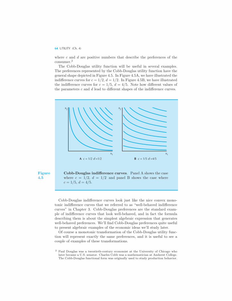
64 UTILITY (Ch. 4)
where c and d are positive numbers that describe the preferences of theconsumer.2
The Cobb-Douglas utility function will be useful in several examples.The preferences represented by the Cobb-Douglas utility function have thegeneral shape depicted in Figure 4.5. In Figure 4.5A, we have illustrated theindifference curves for c = 1/2, d = 1/2. In Figure 4.5B, we have illustratedthe indifference curves for c = 1/5, d = 4/5. Note how different values ofthe parameters c and d lead to different shapes of the indifference curves.
x2 x2
x1
B c = 1/5 d =4/5
1x
A c = 1/2 d =1/2
Figure4.5
Cobb-Douglas indifference curves. Panel A shows the casewhere c = 1/2, d = 1/2 and panel B shows the case wherec = 1/5, d = 4/5.
Cobb-Douglas indifference curves look just like the nice convex mono-tonic indifference curves that we referred to as “well-behaved indifferencecurves” in Chapter 3. Cobb-Douglas preferences are the standard exam-ple of indifference curves that look well-behaved, and in fact the formuladescribing them is about the simplest algebraic expression that generateswell-behaved preferences. We’ll find Cobb-Douglas preferences quite usefulto present algebraic examples of the economic ideas we’ll study later.Of course a monotonic transformation of the Cobb-Douglas utility func-
tion will represent exactly the same preferences, and it is useful to see acouple of examples of these transformations.
2 Paul Douglas was a twentieth-century economist at the University of Chicago wholater became a U.S. senator. Charles Cobb was a mathematician at Amherst College.The Cobb-Douglas functional form was originally used to study production behavior.
MARGINAL UTILITY 65
First, if we take the natural log of utility, the product of the terms willbecome a sum so that we have
v(x1, x2) = ln(xc1x
d2) = c lnx1 + d lnx2.
The indifference curves for this utility function will look just like the onesfor the first Cobb-Douglas function, since the logarithm is a monotonictransformation. (For a brief review of natural logarithms, see the Mathe-matical Appendix at the end of the book.)For the second example, suppose that we start with the Cobb-Douglas
formv(x1, x2) = xc
1xd2.
Then raising utility to the 1/(c+ d) power, we have
xc
c+d
1 xd
c+d
2 .
Now define a new numbera =
c
c+ d.
We can now write our utility function as
v(x1, x2) = xa1x
1−a2 .
This means that we can always take a monotonic transformation of theCobb-Douglas utility function that make the exponents sum to 1. Thiswill turn out to have a useful interpretation later on.The Cobb-Douglas utility function can be expressed in a variety of ways;
you should learn to recognize them, as this family of preferences is veryuseful for examples.
4.4 Marginal Utility
Consider a consumer who is consuming some bundle of goods, (x1, x2).How does this consumer’s utility change as we give him or her a little moreof good 1? This rate of change is called the marginal utility with respectto good 1. We write it as MU1 and think of it as being a ratio,
MU1 =ΔU
Δx1=
u(x1 +Δx1, x2)− u(x1, x2)
Δx1,
that measures the rate of change in utility (ΔU) associated with a smallchange in the amount of good 1 (Δx1). Note that the amount of good 2 isheld fixed in this calculation.3
3 See the appendix to this chapter for a calculus treatment of marginal utility.
66 UTILITY (Ch. 4)
This definition implies that to calculate the change in utility associatedwith a small change in consumption of good 1, we can just multiply thechange in consumption by the marginal utility of the good:
ΔU = MU1Δx1.
The marginal utility with respect to good 2 is defined in a similar manner:
MU2 =ΔU
Δx2=
u(x1, x2 +Δx2)− u(x1, x2)
Δx2.
Note that when we compute the marginal utility with respect to good 2 wekeep the amount of good 1 constant. We can calculate the change in utilityassociated with a change in the consumption of good 2 by the formula
ΔU = MU2Δx2.
It is important to realize that the magnitude of marginal utility dependson the magnitude of utility. Thus it depends on the particular way that wechoose to measure utility. If we multiplied utility by 2, then marginal utilitywould also be multiplied by 2. We would still have a perfectly valid utilityfunction in that it would represent the same preferences, but it would justbe scaled differently.This means that marginal utility itself has no behavioral content. How
can we calculate marginal utility from a consumer’s choice behavior? Wecan’t. Choice behavior only reveals information about the way a consumerranks different bundles of goods. Marginal utility depends on the partic-ular utility function that we use to reflect the preference ordering and itsmagnitude has no particular significance. However, it turns out that mar-ginal utility can be used to calculate something that does have behavioralcontent, as we will see in the next section.
4.5 Marginal Utility and MRS
A utility function u(x1, x2) can be used to measure the marginal rate ofsubstitution (MRS) defined in Chapter 3. Recall that the MRS measuresthe slope of the indifference curve at a given bundle of goods; it can beinterpreted as the rate at which a consumer is just willing to substitute asmall amount of good 2 for good 1.This interpretation gives us a simple way to calculate the MRS. Con-
sider a change in the consumption of each good, (Δx1,Δx2), that keepsutility constant—that is, a change in consumption that moves us along theindifference curve. Then we must have
MU1Δx1 +MU2Δx2 = ΔU = 0.
UTILITY FOR COMMUTING 67
Solving for the slope of the indifference curve we have
MRS =Δx2
Δx1= −MU1
MU2. (4.1)
(Note that we have 2 over 1 on the left-hand side of the equation and 1over 2 on the right-hand side. Don’t get confused!)The algebraic sign of the MRS is negative: if you get more of good 1 you
have to get less of good 2 in order to keep the same level of utility. However,it gets very tedious to keep track of that pesky minus sign, so economistsoften refer to the MRS by its absolute value—that is, as a positive number.We’ll follow this convention as long as no confusion will result.Now here is the interesting thing about the MRS calculation: the MRS
can be measured by observing a person’s actual behavior—we find thatrate of exchange where he or she is just willing to stay put, as described inChapter 3.The utility function, and therefore the marginal utility function, is not
uniquely determined. Any monotonic transformation of a utility functionleaves you with another equally valid utility function. Thus, if we multiplyutility by 2, for example, the marginal utility is multiplied by 2. Thus themagnitude of the marginal utility function depends on the choice of utilityfunction, which is arbitrary. It doesn’t depend on behavior alone; insteadit depends on the utility function that we use to describe behavior.But the ratio of marginal utilities gives us an observable magnitude—
namely the marginal rate of substitution. The ratio of marginal utilitiesis independent of the particular transformation of the utility function youchoose to use. Look at what happens if you multiply utility by 2. TheMRS becomes
MRS = −2MU1
2MU2.
The 2s just cancel out, so the MRS remains the same.The same sort of thing occurs when we take any monotonic transforma-
tion of a utility function. Taking a monotonic transformation is just rela-beling the indifference curves, and the calculation for the MRS describedabove is concerned with moving along a given indifference curve. Eventhough the marginal utilities are changed by monotonic transformations,the ratio of marginal utilities is independent of the particular way chosento represent the preferences.
4.6 Utility for Commuting
Utility functions are basically ways of describing choice behavior: if a bun-dle of goods X is chosen when a bundle of goods Y is available, then Xmust have a higher utility than Y . By examining choices consumers makewe can estimate a utility function to describe their behavior.
68 UTILITY (Ch. 4)
This idea has been widely applied in the field of transportation economicsto study consumers’ commuting behavior. In most large cities commutershave a choice between taking public transit or driving to work. Each ofthese alternatives can be thought of as representing a bundle of differentcharacteristics: travel time, waiting time, out-of-pocket costs, comfort, con-venience, and so on. We could let x1 be the amount of travel time involvedin each kind of transportation, x2 the amount of waiting time for each kind,and so on.If (x1, x2, . . . , xn) represents the values of n different characteristics of
driving, say, and (y1, y2, . . . , yn) represents the values of taking the bus, wecan consider a model where the consumer decides to drive or take the busdepending on whether he prefers one bundle of characteristics to the other.More specifically, let us suppose that the average consumer’s preferences
for characteristics can be represented by a utility function of the form
U(x1, x2, . . . , xn) = β1x1 + β2x2 + · · ·+ βnxn,
where the coefficients β1, β2, and so on are unknown parameters. Anymonotonic transformation of this utility function would describe the choicebehavior equally well, of course, but the linear form is especially easy towork with from a statistical point of view.Suppose now that we observe a number of similar consumers making
choices between driving and taking the bus based on the particular patternof commute times, costs, and so on that they face. There are statisticaltechniques that can be used to find the values of the coefficients βi for i =1, . . . , n that best fit the observed pattern of choices by a set of consumers.These statistical techniques give a way to estimate the utility function fordifferent transportation modes.One study reports a utility function that had the form4
U(TW, TT,C) = −0.147TW − 0.0411TT − 2.24C, (4.2)
where
TW = total walking time to and from bus or carTT = total time of trip in minutesC = total cost of trip in dollars
The estimated utility function in the Domenich-McFadden book correctlydescribed the choice between auto and bus transport for 93 percent of thehouseholds in their sample.
4 See Thomas Domenich and Daniel McFadden, Urban Travel Demand (North-HollandPublishing Company, 1975). The estimation procedure in this book also incorporatedvarious demographic characteristics of the households in addition to the purely eco-nomic variables described here. Daniel McFadden was awarded the Nobel Prize ineconomics in 2000 for his work in developing techniques to estimate models of thissort.
SUMMARY 69
The coefficients on the variables in Equation (4.2) describe the weightthat an average household places on the various characteristics of theircommuting trips; that is, the marginal utility of each characteristic. Theratio of one coefficient to another measures the marginal rate of substitu-tion between one characteristic and another. For example, the ratio of themarginal utility of walking time to the marginal utility of total time indi-cates that walking time is viewed as being roughly 3 times as onerous astravel time by the average consumer. In other words, the consumer wouldbe willing to substitute 3 minutes of additional travel time to save 1 minuteof walking time.Similarly, the ratio of cost to travel time indicates the average consumer’s
tradeoff between these two variables. In this study, the average commutervalued a minute of commute time at 0.0411/2.24 = 0.0183 dollars perminute, which is $1.10 per hour. For comparison, the hourly wage for theaverage commuter in 1967, the year of the study, was about $2.85 an hour.Such estimated utility functions can be very valuable for determining
whether or not it is worthwhile to make some change in the public trans-portation system. For example, in the above utility function one of thesignificant factors explaining mode choice is the time involved in takingthe trip. The city transit authority can, at some cost, add more buses toreduce this travel time. But will the number of extra riders warrant theincreased expense?Given a utility function and a sample of consumers we can forecast which
consumers will drive and which consumers will choose to take the bus. Thiswill give us some idea as to whether the revenue will be sufficient to coverthe extra cost.Furthermore, we can use the marginal rate of substitution to estimate
the value that each consumer places on the reduced travel time. We sawabove that in the Domenich-McFadden study the average commuter in1967 valued commute time at a rate of $1.10 per hour. Thus the commutershould be willing to pay about $0.37 to cut 20 minutes from his or hertrip. This number gives us a measure of the dollar benefit of providingmore timely bus service. This benefit must be compared to the cost ofproviding more timely bus service in order to determine if such provisionis worthwhile. Having a quantitative measure of benefit will certainly behelpful in making a rational decision about transport policy.
Summary
1. A utility function is simply a way to represent or summarize a prefer-ence ordering. The numerical magnitudes of utility levels have no intrinsicmeaning.
2. Thus, given any one utility function, any monotonic transformation ofit will represent the same preferences.
70 UTILITY (Ch. 4)
3. The marginal rate of substitution, MRS, can be calculated from theutility function via the formula MRS = Δx2/Δx1 = −MU1/MU2.
REVIEW QUESTIONS
1. The text said that raising a number to an odd power was a monotonictransformation. What about raising a number to an even power? Is this amonotonic transformation? (Hint: consider the case f(u) = u2.)
2. Which of the following are monotonic transformations? (1) u = 2v− 13;(2) u = −1/v2; (3) u = 1/v2; (4) u = ln v; (5) u = −e−v; (6) u = v2;(7) u = v2 for v > 0; (8) u = v2 for v < 0.
3. We claimed in the text that if preferences were monotonic, then a diag-onal line through the origin would intersect each indifference curve exactlyonce. Can you prove this rigorously? (Hint: what would happen if itintersected some indifference curve twice?)
4. What kind of preferences are represented by a utility function of theform u(x1, x2) =
√x1 + x2? What about the utility function v(x1, x2) =
13x1 + 13x2?
5. What kind of preferences are represented by a utility function of the formu(x1, x2) = x1 +
√x2? Is the utility function v(x1, x2) = x2
1+2x1√x2 +x2
a monotonic transformation of u(x1, x2)?
6. Consider the utility function u(x1, x2) =√x1x2. What kind of pref-
erences does it represent? Is the function v(x1, x2) = x21x2 a monotonic
transformation of u(x1, x2)? Is the function w(x1, x2) = x21x
22 a monotonic
transformation of u(x1, x2)?
7. Can you explain why taking a monotonic transformation of a utilityfunction doesn’t change the marginal rate of substitution?
APPENDIX
First, let us clarify what is meant by “marginal utility.” As elsewhere in eco-nomics, “marginal” just means a derivative. So the marginal utility of good 1 isjust
MU1 = limΔx1→0
u(x1 +Δx1, x2)− u(x1, x2)
Δx1=
∂u(x1, x2)
∂x1.
Note that we have used the partial derivative here, since the marginal utilityof good 1 is computed holding good 2 fixed.
APPENDIX 71
Now we can rephrase the derivation of the MRS given in the text using calculus.We’ll do it two ways: first by using differentials, and second by using implicitfunctions.
For the first method, we consider making a change (dx1, dx2) that keeps utilityconstant. So we want
du =∂u(x1, x2)
∂x1dx1 +
∂u(x1, x2)
∂x2dx2 = 0.
The first term measures the increase in utility from the small change dx1, andthe second term measures the increase in utility from the small change dx2. Wewant to pick these changes so that the total change in utility, du, is zero. Solvingfor dx2/dx1 gives us
dx2
dx1= −∂u(x1, x2)/∂x1
∂u(x1, x2)/∂x2,
which is just the calculus analog of equation (4.1) in the text.As for the second method, we now think of the indifference curve as being
described by a function x2(x1). That is, for each value of x1, the function x2(x1)tells us how much x2 we need to get on that specific indifference curve. Thus thefunction x2(x1) has to satisfy the identity
u(x1, x2(x1)) ≡ k,
where k is the utility label of the indifference curve in question.We can differentiate both sides of this identity with respect to x1 to get
∂u(x1, x2)
∂x1+
∂u(x1, x2)
∂x2
∂x2(x1)
∂x1= 0.
Notice that x1 occurs in two places in this identity, so changing x1 will changethe function in two ways, and we have to take the derivative at each place thatx1 appears.
We then solve this equation for ∂x2(x1)/∂x1 to find
∂x2(x1)
∂x1= −∂u(x1, x2)/∂x1
∂u(x1, x2)/∂x2,
just as we had before.The implicit function method is a little more rigorous, but the differential
method is more direct, as long as you don’t do something silly.Suppose that we take a monotonic transformation of a utility function, say,
v(x1, x2) = f(u(x1, x2)). Let’s calculate the MRS for this utility function. Usingthe chain rule
MRS = −∂v/∂x1
∂v/∂x2= −∂f/∂u
∂f/∂u
∂u/∂x1
∂u/∂x2
= −∂u/∂x1
∂u/∂x2
since the ∂f/∂u term cancels out from both the numerator and denominator.This shows that the MRS is independent of the utility representation.
This gives a useful way to recognize preferences that are represented by dif-ferent utility functions: given two utility functions, just compute the marginalrates of substitution and see if they are the same. If they are, then the twoutility functions have the same indifference curves. If the direction of increasingpreference is the same for each utility function, then the underlying preferencesmust be the same.
72 UTILITY (Ch. 4)
EXAMPLE: Cobb-Douglas Preferences
The MRS for Cobb-Douglas preferences is easy to calculate by using the formuladerived above.
If we choose the log representation where
u(x1, x2) = c lnx1 + d lnx2,
then we have
MRS = −∂u(x1, x2)/∂x1
∂u(x1, x2)/∂x2
= − c/x1
d/x2
= − c
d
x2
x1.
Note that the MRS only depends on the ratio of the two parameters and thequantity of the two goods in this case.
What if we choose the exponent representation where
u(x1, x2) = xc1x
d2?
Then we have
MRS = −∂u(x1, x2)/∂x1
∂u(x1, x2)/∂x2
= − cxc−11 xd
2
dxc1x
d−12
= − cx2
dx1,
which is the same as we had before. Of course you knew all along that a monotonictransformation couldn’t change the marginal rate of substitution!

CHAPTER 5
CHOICE
In this chapter we will put together the budget set and the theory of prefer-ences in order to examine the optimal choice of consumers. We said earlierthat the economic model of consumer choice is that people choose the bestbundle they can afford. We can now rephrase this in terms that sound moreprofessional by saying that “consumers choose the most preferred bundlefrom their budget sets.”
5.1 Optimal Choice
A typical case is illustrated in Figure 5.1. Here we have drawn the budgetset and several of the consumer’s indifference curves on the same diagram.We want to find the bundle in the budget set that is on the highest indif-ference curve. Since preferences are well-behaved, so that more is preferredto less, we can restrict our attention to bundles of goods that lie on thebudget line and not worry about those beneath the budget line.Now simply start at the right-hand corner of the budget line and move to
the left. As we move along the budget line we note that we are moving tohigher and higher indifference curves. We stop when we get to the highest
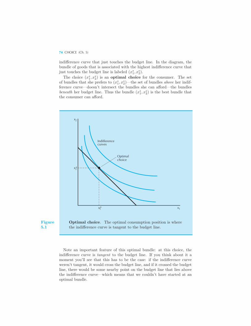
74 CHOICE (Ch. 5)
indifference curve that just touches the budget line. In the diagram, thebundle of goods that is associated with the highest indifference curve thatjust touches the budget line is labeled (x∗
1, x∗2).
The choice (x∗1, x
∗2) is an optimal choice for the consumer. The set
of bundles that she prefers to (x∗1, x
∗2)—the set of bundles above her indif-
ference curve—doesn’t intersect the bundles she can afford—the bundlesbeneath her budget line. Thus the bundle (x∗
1, x∗2) is the best bundle that
the consumer can afford.
x2
Indifferencecurves
Optimalchoice
x*2
x* x1 1
Figure5.1
Optimal choice. The optimal consumption position is wherethe indifference curve is tangent to the budget line.
Note an important feature of this optimal bundle: at this choice, theindifference curve is tangent to the budget line. If you think about it amoment you’ll see that this has to be the case: if the indifference curveweren’t tangent, it would cross the budget line, and if it crossed the budgetline, there would be some nearby point on the budget line that lies abovethe indifference curve—which means that we couldn’t have started at anoptimal bundle.
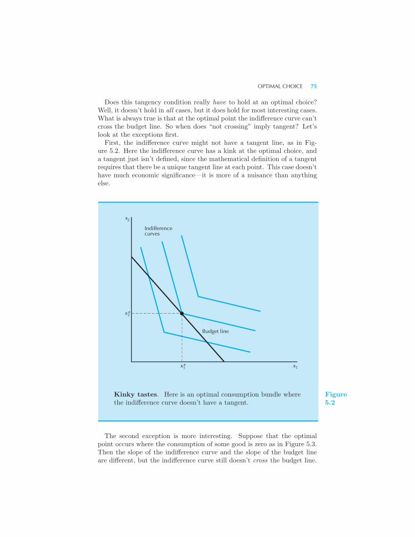
OPTIMAL CHOICE 75
Does this tangency condition really have to hold at an optimal choice?Well, it doesn’t hold in all cases, but it does hold for most interesting cases.What is always true is that at the optimal point the indifference curve can’tcross the budget line. So when does “not crossing” imply tangent? Let’slook at the exceptions first.First, the indifference curve might not have a tangent line, as in Fig-
ure 5.2. Here the indifference curve has a kink at the optimal choice, anda tangent just isn’t defined, since the mathematical definition of a tangentrequires that there be a unique tangent line at each point. This case doesn’thave much economic significance—it is more of a nuisance than anythingelse.
x2
2x*
1x* x1
Budget line
Indifferencecurves
Kinky tastes. Here is an optimal consumption bundle wherethe indifference curve doesn’t have a tangent.
Figure5.2
The second exception is more interesting. Suppose that the optimalpoint occurs where the consumption of some good is zero as in Figure 5.3.Then the slope of the indifference curve and the slope of the budget lineare different, but the indifference curve still doesn’t cross the budget line.
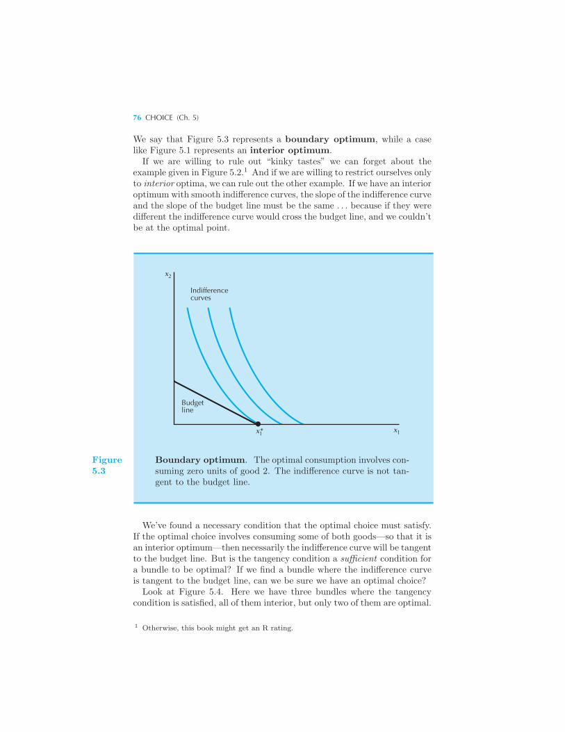
76 CHOICE (Ch. 5)
We say that Figure 5.3 represents a boundary optimum, while a caselike Figure 5.1 represents an interior optimum.If we are willing to rule out “kinky tastes” we can forget about the
example given in Figure 5.2.1 And if we are willing to restrict ourselves onlyto interior optima, we can rule out the other example. If we have an interioroptimum with smooth indifference curves, the slope of the indifference curveand the slope of the budget line must be the same . . . because if they weredifferent the indifference curve would cross the budget line, and we couldn’tbe at the optimal point.
2
Indifferencecurves
x
Budgetline
x* x11
Figure5.3
Boundary optimum. The optimal consumption involves con-suming zero units of good 2. The indifference curve is not tan-gent to the budget line.
We’ve found a necessary condition that the optimal choice must satisfy.If the optimal choice involves consuming some of both goods—so that it isan interior optimum—then necessarily the indifference curve will be tangentto the budget line. But is the tangency condition a sufficient condition fora bundle to be optimal? If we find a bundle where the indifference curveis tangent to the budget line, can we be sure we have an optimal choice?Look at Figure 5.4. Here we have three bundles where the tangency
condition is satisfied, all of them interior, but only two of them are optimal.
1 Otherwise, this book might get an R rating.
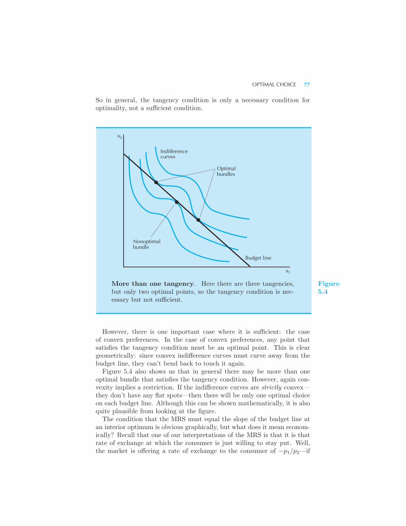
OPTIMAL CHOICE 77
So in general, the tangency condition is only a necessary condition foroptimality, not a sufficient condition.
x2
Indifferencecurves
Optimalbundles
Nonoptimalbundle
Budget line
x1
More than one tangency. Here there are three tangencies,but only two optimal points, so the tangency condition is nec-essary but not sufficient.
Figure5.4
However, there is one important case where it is sufficient: the caseof convex preferences. In the case of convex preferences, any point thatsatisfies the tangency condition must be an optimal point. This is cleargeometrically: since convex indifference curves must curve away from thebudget line, they can’t bend back to touch it again.Figure 5.4 also shows us that in general there may be more than one
optimal bundle that satisfies the tangency condition. However, again con-vexity implies a restriction. If the indifference curves are strictly convex—they don’t have any flat spots—then there will be only one optimal choiceon each budget line. Although this can be shown mathematically, it is alsoquite plausible from looking at the figure.The condition that the MRS must equal the slope of the budget line at
an interior optimum is obvious graphically, but what does it mean econom-ically? Recall that one of our interpretations of the MRS is that it is thatrate of exchange at which the consumer is just willing to stay put. Well,the market is offering a rate of exchange to the consumer of −p1/p2—if
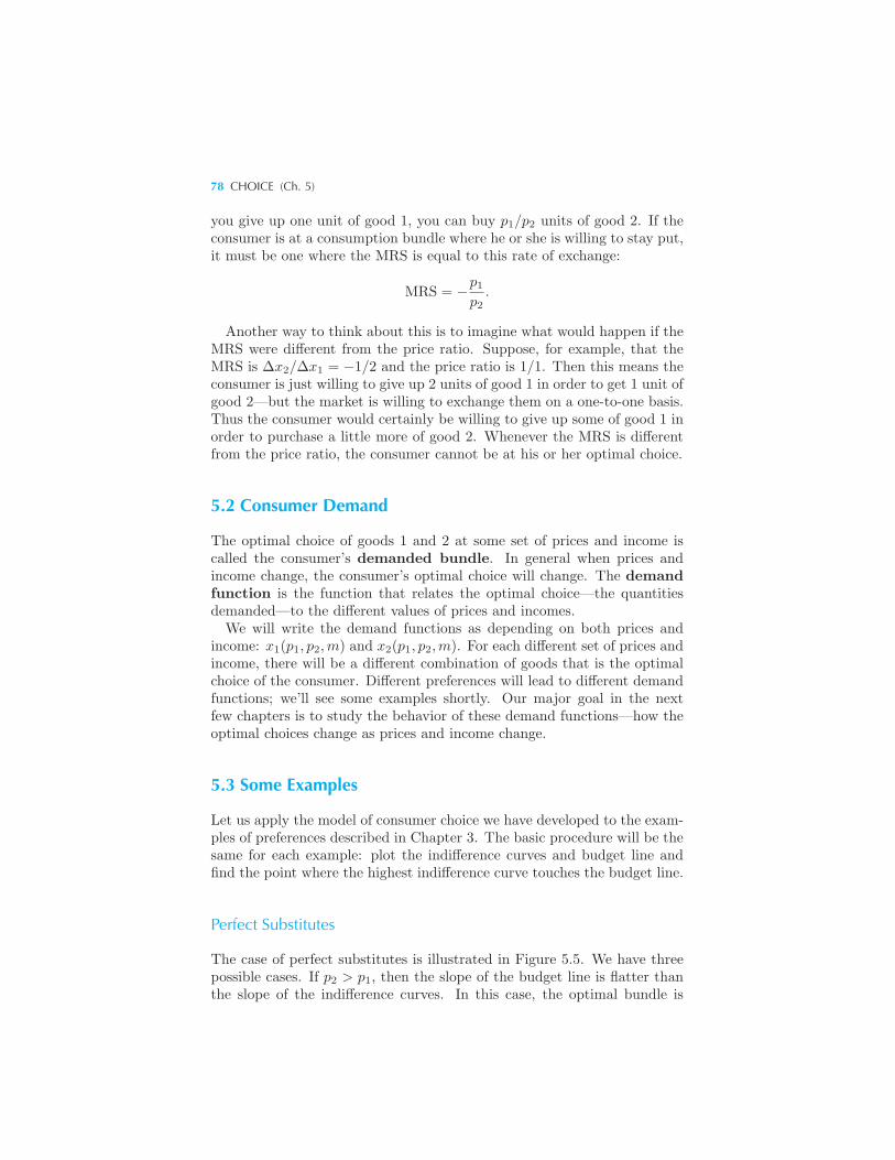
78 CHOICE (Ch. 5)
you give up one unit of good 1, you can buy p1/p2 units of good 2. If theconsumer is at a consumption bundle where he or she is willing to stay put,it must be one where the MRS is equal to this rate of exchange:
MRS = −p1p2
.
Another way to think about this is to imagine what would happen if theMRS were different from the price ratio. Suppose, for example, that theMRS is Δx2/Δx1 = −1/2 and the price ratio is 1/1. Then this means theconsumer is just willing to give up 2 units of good 1 in order to get 1 unit ofgood 2—but the market is willing to exchange them on a one-to-one basis.Thus the consumer would certainly be willing to give up some of good 1 inorder to purchase a little more of good 2. Whenever the MRS is differentfrom the price ratio, the consumer cannot be at his or her optimal choice.
5.2 Consumer Demand
The optimal choice of goods 1 and 2 at some set of prices and income iscalled the consumer’s demanded bundle. In general when prices andincome change, the consumer’s optimal choice will change. The demandfunction is the function that relates the optimal choice—the quantitiesdemanded—to the different values of prices and incomes.We will write the demand functions as depending on both prices and
income: x1(p1, p2,m) and x2(p1, p2,m). For each different set of prices andincome, there will be a different combination of goods that is the optimalchoice of the consumer. Different preferences will lead to different demandfunctions; we’ll see some examples shortly. Our major goal in the nextfew chapters is to study the behavior of these demand functions—how theoptimal choices change as prices and income change.
5.3 Some Examples
Let us apply the model of consumer choice we have developed to the exam-ples of preferences described in Chapter 3. The basic procedure will be thesame for each example: plot the indifference curves and budget line andfind the point where the highest indifference curve touches the budget line.
Perfect Substitutes
The case of perfect substitutes is illustrated in Figure 5.5. We have threepossible cases. If p2 > p1, then the slope of the budget line is flatter thanthe slope of the indifference curves. In this case, the optimal bundle is
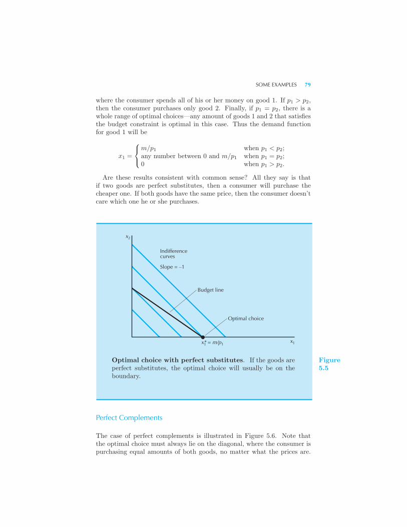
SOME EXAMPLES 79
where the consumer spends all of his or her money on good 1. If p1 > p2,then the consumer purchases only good 2. Finally, if p1 = p2, there is awhole range of optimal choices—any amount of goods 1 and 2 that satisfiesthe budget constraint is optimal in this case. Thus the demand functionfor good 1 will be
x1 =
⎧⎨⎩
m/p1 when p1 < p2;any number between 0 and m/p1 when p1 = p2;0 when p1 > p2.
Are these results consistent with common sense? All they say is thatif two goods are perfect substitutes, then a consumer will purchase thecheaper one. If both goods have the same price, then the consumer doesn’tcare which one he or she purchases.
x2
Indifferencecurves
Slope = –1
Budget line
Optimal choice
x* = m/p x11 1
Optimal choice with perfect substitutes. If the goods areperfect substitutes, the optimal choice will usually be on theboundary.
Figure5.5
Perfect Complements
The case of perfect complements is illustrated in Figure 5.6. Note thatthe optimal choice must always lie on the diagonal, where the consumer ispurchasing equal amounts of both goods, no matter what the prices are.
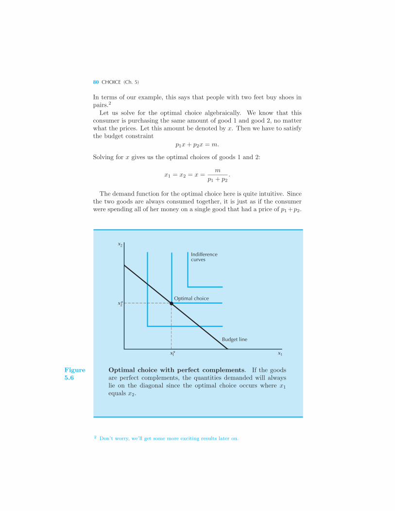
80 CHOICE (Ch. 5)
In terms of our example, this says that people with two feet buy shoes inpairs.2
Let us solve for the optimal choice algebraically. We know that thisconsumer is purchasing the same amount of good 1 and good 2, no matterwhat the prices. Let this amount be denoted by x. Then we have to satisfythe budget constraint
p1x+ p2x = m.
Solving for x gives us the optimal choices of goods 1 and 2:
x1 = x2 = x =m
p1 + p2.
The demand function for the optimal choice here is quite intuitive. Sincethe two goods are always consumed together, it is just as if the consumerwere spending all of her money on a single good that had a price of p1+p2.
Indifferencecurves
Optimal choicex*
x2
2
Budget line
x*1 1x
Figure5.6
Optimal choice with perfect complements. If the goodsare perfect complements, the quantities demanded will alwayslie on the diagonal since the optimal choice occurs where x1
equals x2.
2 Don’t worry, we’ll get some more exciting results later on.
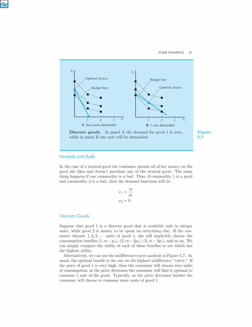
SOME EXAMPLES 81
B 1 unit demanded
1 2 3
A Zero units demanded
1 2 3
Optimal choice
Budget line Optimal choice
Budget line
x2 x2
x1 x1
Discrete goods. In panel A the demand for good 1 is zero,while in panel B one unit will be demanded.
Figure5.7
Neutrals and Bads
In the case of a neutral good the consumer spends all of her money on thegood she likes and doesn’t purchase any of the neutral good. The samething happens if one commodity is a bad. Thus, if commodity 1 is a goodand commodity 2 is a bad, then the demand functions will be
x1 =m
p1
x2 = 0.
Discrete Goods
Suppose that good 1 is a discrete good that is available only in integerunits, while good 2 is money to be spent on everything else. If the con-sumer chooses 1, 2, 3, · · · units of good 1, she will implicitly choose theconsumption bundles (1,m− p1), (2,m− 2p1), (3,m− 3p1), and so on. Wecan simply compare the utility of each of these bundles to see which hasthe highest utility.Alternatively, we can use the indifference-curve analysis in Figure 5.7. As
usual, the optimal bundle is the one on the highest indifference “curve.” Ifthe price of good 1 is very high, then the consumer will choose zero unitsof consumption; as the price decreases the consumer will find it optimal toconsume 1 unit of the good. Typically, as the price decreases further theconsumer will choose to consume more units of good 1.
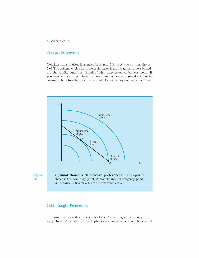
82 CHOICE (Ch. 5)
Concave Preferences
Consider the situation illustrated in Figure 5.8. Is X the optimal choice?No! The optimal choice for these preferences is always going to be a bound-ary choice, like bundle Z. Think of what nonconvex preferences mean. Ifyou have money to purchase ice cream and olives, and you don’t like toconsume them together, you’ll spend all of your money on one or the other.
x2
Nonoptimalchoice
Indifferencecurves
XBudgetline
Optimalchoice
Z x1
Figure5.8
Optimal choice with concave preferences. The optimalchoice is the boundary point, Z, not the interior tangency point,X, because Z lies on a higher indifference curve.
Cobb-Douglas Preferences
Suppose that the utility function is of the Cobb-Douglas form, u(x1, x2) =xc1x
d2. In the Appendix to this chapter we use calculus to derive the optimal
ESTIMATING UTILITY FUNCTIONS 83
choices for this utility function. They turn out to be
x1 =c
c+ d
m
p1
x2 =d
c+ d
m
p2.
These demand functions are often useful in algebraic examples, so youshould probably memorize them.The Cobb-Douglas preferences have a convenient property. Consider the
fraction of his income that a Cobb-Douglas consumer spends on good 1. Ifhe consumes x1 units of good 1, this costs him p1x1, so this represents afraction p1x1/m of total income. Substituting the demand function for x1
we havep1x1
m=
p1m
c
c+ d
m
p1=
c
c+ d.
Similarly the fraction of his income that the consumer spends on good 2 isd/(c+ d).Thus the Cobb-Douglas consumer always spends a fixed fraction of his
income on each good. The size of the fraction is determined by the exponentin the Cobb-Douglas function.This is why it is often convenient to choose a representation of the Cobb-
Douglas utility function in which the exponents sum to 1. If u(x1, x2) =xa1x
1−a2 , then we can immediately interpret a as the fraction of income spent
on good 1. For this reason we will usually write Cobb-Douglas preferencesin this form.
5.4 Estimating Utility Functions
We’ve now seen several different forms for preferences and utility functionsand have examined the kinds of demand behavior generated by these pref-erences. But in real life we usually have to work the other way around: weobserve demand behavior, but our problem is to determine what kind ofpreferences generated the observed behavior.For example, suppose that we observe a consumer’s choices at several
different prices and income levels. An example is depicted in Table 5.1.This is a table of the demand for two goods at the different levels of pricesand incomes that prevailed in different years. We have also computedthe share of income spent on each good in each year using the formulass1 = p1x1/m and s2 = p2x2/m.
For these data, the expenditure shares are relatively constant. There aresmall variations from observation to observation, but they probably aren’tlarge enough to worry about. The average expenditure share for good 1 isabout 1/4, and the average income share for good 2 is about 3/4. It appears
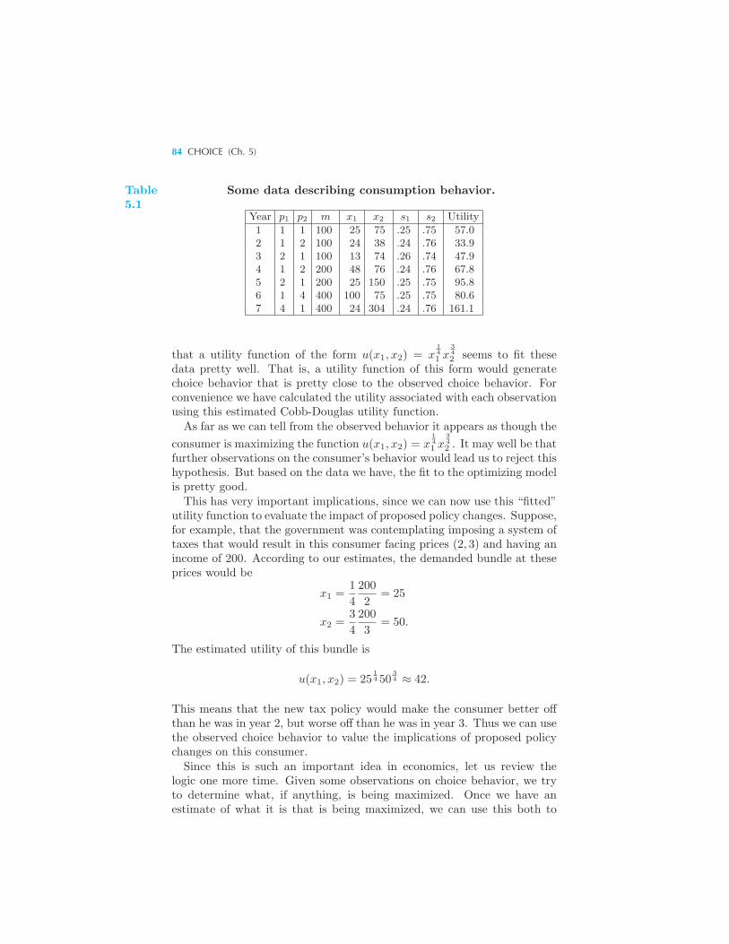
84 CHOICE (Ch. 5)
Table5.1
Some data describing consumption behavior.
Year p1 p2 m x1 x2 s1 s2 Utility
1 1 1 100 25 75 .25 .75 57.02 1 2 100 24 38 .24 .76 33.93 2 1 100 13 74 .26 .74 47.94 1 2 200 48 76 .24 .76 67.85 2 1 200 25 150 .25 .75 95.86 1 4 400 100 75 .25 .75 80.67 4 1 400 24 304 .24 .76 161.1
that a utility function of the form u(x1, x2) = x141 x
342 seems to fit these
data pretty well. That is, a utility function of this form would generatechoice behavior that is pretty close to the observed choice behavior. Forconvenience we have calculated the utility associated with each observationusing this estimated Cobb-Douglas utility function.As far as we can tell from the observed behavior it appears as though the
consumer is maximizing the function u(x1, x2) = x141 x
342 . It may well be that
further observations on the consumer’s behavior would lead us to reject thishypothesis. But based on the data we have, the fit to the optimizing modelis pretty good.This has very important implications, since we can now use this “fitted”
utility function to evaluate the impact of proposed policy changes. Suppose,for example, that the government was contemplating imposing a system oftaxes that would result in this consumer facing prices (2, 3) and having anincome of 200. According to our estimates, the demanded bundle at theseprices would be
x1 =1
4
200
2= 25
x2 =3
4
200
3= 50.
The estimated utility of this bundle is
u(x1, x2) = 2514 50
34 ≈ 42.
This means that the new tax policy would make the consumer better offthan he was in year 2, but worse off than he was in year 3. Thus we can usethe observed choice behavior to value the implications of proposed policychanges on this consumer.Since this is such an important idea in economics, let us review the
logic one more time. Given some observations on choice behavior, we tryto determine what, if anything, is being maximized. Once we have anestimate of what it is that is being maximized, we can use this both to
IMPLICATIONS OF THE MRS CONDITION 85
predict choice behavior in new situations and to evaluate proposed changesin the economic environment.Of course we have described a very simple situation. In reality, we nor-
mally don’t have detailed data on individual consumption choices. But weoften have data on groups of individuals—teenagers, middle-class house-holds, elderly people, and so on. These groups may have different prefer-ences for different goods that are reflected in their patterns of consumptionexpenditure. We can estimate a utility function that describes their con-sumption patterns and then use this estimated utility function to forecastdemand and evaluate policy proposals.In the simple example described above, it was apparent that income
shares were relatively constant so that the Cobb-Douglas utility functionwould give us a pretty good fit. In other cases, a more complicated formfor the utility function would be appropriate. The calculations may thenbecome messier, and we may need to use a computer for the estimation,but the essential idea of the procedure is the same.
5.5 Implications of the MRS Condition
In the last section we examined the important idea that observation of de-mand behavior tells us important things about the underlying preferencesof the consumers that generated that behavior. Given sufficient observa-tions on consumer choices it will often be possible to estimate the utilityfunction that generated those choices.But even observing one consumer choice at one set of prices will allow
us to make some kinds of useful inferences about how consumer utility willchange when consumption changes. Let us see how this works.In well-organized markets, it is typical that everyone faces roughly the
same prices for goods. Take, for example, two goods like butter and milk.If everyone faces the same prices for butter and milk, and everyone isoptimizing, and everyone is at an interior solution . . . then everyone musthave the same marginal rate of substitution for butter and milk.This follows directly from the analysis given above. The market is offer-
ing everyone the same rate of exchange for butter and milk, and everyoneis adjusting their consumption of the goods until their own “internal” mar-ginal valuation of the two goods equals the market’s “external” valuationof the two goods.Now the interesting thing about this statement is that it is independent
of income and tastes. People may value their total consumption of the twogoods very differently. Some people may be consuming a lot of butter anda little milk, and some may be doing the reverse. Some wealthy peoplemay be consuming a lot of milk and a lot of butter while other people maybe consuming just a little of each good. But everyone who is consumingthe two goods must have the same marginal rate of substitution. Everyone
86 CHOICE (Ch. 5)
who is consuming the goods must agree on how much one is worth in termsof the other: how much of one they would be willing to sacrifice to get somemore of the other.The fact that price ratios measure marginal rates of substitution is very
important, for it means that we have a way to value possible changes inconsumption bundles. Suppose, for example, that the price of milk is $1a quart and the price of butter is $2 a pound. Then the marginal rate ofsubstitution for all people who consume milk and butter must be 2: theyhave to have 2 quarts of milk to compensate them for giving up 1 poundof butter. Or conversely, they have to have 1 pound of butter to makeit worth their while to give up 2 quarts of milk. Hence everyone who isconsuming both goods will value a marginal change in consumption in thesame way.Now suppose that an inventor discovers a new way of turning milk into
butter: for every 3 quarts of milk poured into this machine, you get out1 pound of butter, and no other useful byproducts. Question: is therea market for this device? Answer: the venture capitalists won’t beat apath to his door, that’s for sure. For everyone is already operating at apoint where they are just willing to trade 2 quarts of milk for 1 poundof butter; why would they be willing to substitute 3 quarts of milk for 1pound of butter? The answer is they wouldn’t; this invention isn’t worthanything.But what would happen if he got it to run in reverse so he could dump
in a pound of butter get out 3 quarts of milk? Is there a market for thisdevice? Answer: yes! The market prices of milk and butter tell us thatpeople are just barely willing to trade one pound of butter for 2 quarts ofmilk. So getting 3 quarts of milk for a pound of butter is a better deal thanis currently being offered in the marketplace. Sign me up for a thousandshares! (And several pounds of butter.)The market prices show that the first machine is unprofitable: it produces
$2 of butter by using $3 of milk. The fact that it is unprofitable is justanother way of saying that people value the inputs more than the outputs.The second machine produces $3 worth of milk by using only $2 worth ofbutter. This machine is profitable because people value the outputs morethan the inputs.The point is that, since prices measure the rate at which people are just
willing to substitute one good for another, they can be used to value policyproposals that involve making changes in consumption. The fact that pricesare not arbitrary numbers but reflect how people value things on the marginis one of the most fundamental and important ideas in economics.If we observe one choice at one set of prices we get the MRS at one
consumption point. If the prices change and we observe another choice weget another MRS. As we observe more and more choices we learn moreand more about the shape of the underlying preferences that may havegenerated the observed choice behavior.
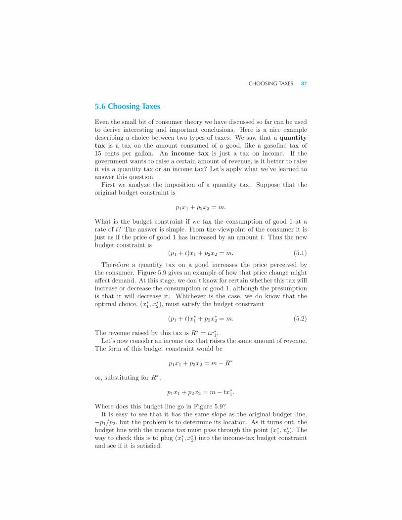
CHOOSING TAXES 87
5.6 Choosing Taxes
Even the small bit of consumer theory we have discussed so far can be usedto derive interesting and important conclusions. Here is a nice exampledescribing a choice between two types of taxes. We saw that a quantitytax is a tax on the amount consumed of a good, like a gasoline tax of15 cents per gallon. An income tax is just a tax on income. If thegovernment wants to raise a certain amount of revenue, is it better to raiseit via a quantity tax or an income tax? Let’s apply what we’ve learned toanswer this question.First we analyze the imposition of a quantity tax. Suppose that the
original budget constraint is
p1x1 + p2x2 = m.
What is the budget constraint if we tax the consumption of good 1 at arate of t? The answer is simple. From the viewpoint of the consumer it isjust as if the price of good 1 has increased by an amount t. Thus the newbudget constraint is
(p1 + t)x1 + p2x2 = m. (5.1)
Therefore a quantity tax on a good increases the price perceived bythe consumer. Figure 5.9 gives an example of how that price change mightaffect demand. At this stage, we don’t know for certain whether this tax willincrease or decrease the consumption of good 1, although the presumptionis that it will decrease it. Whichever is the case, we do know that theoptimal choice, (x∗
1, x∗2), must satisfy the budget constraint
(p1 + t)x∗1 + p2x
∗2 = m. (5.2)
The revenue raised by this tax is R∗ = tx∗1.
Let’s now consider an income tax that raises the same amount of revenue.The form of this budget constraint would be
p1x1 + p2x2 = m−R∗
or, substituting for R∗,
p1x1 + p2x2 = m− tx∗1.
Where does this budget line go in Figure 5.9?It is easy to see that it has the same slope as the original budget line,
−p1/p2, but the problem is to determine its location. As it turns out, thebudget line with the income tax must pass through the point (x∗
1, x∗2). The
way to check this is to plug (x∗1, x
∗2) into the income-tax budget constraint
and see if it is satisfied.
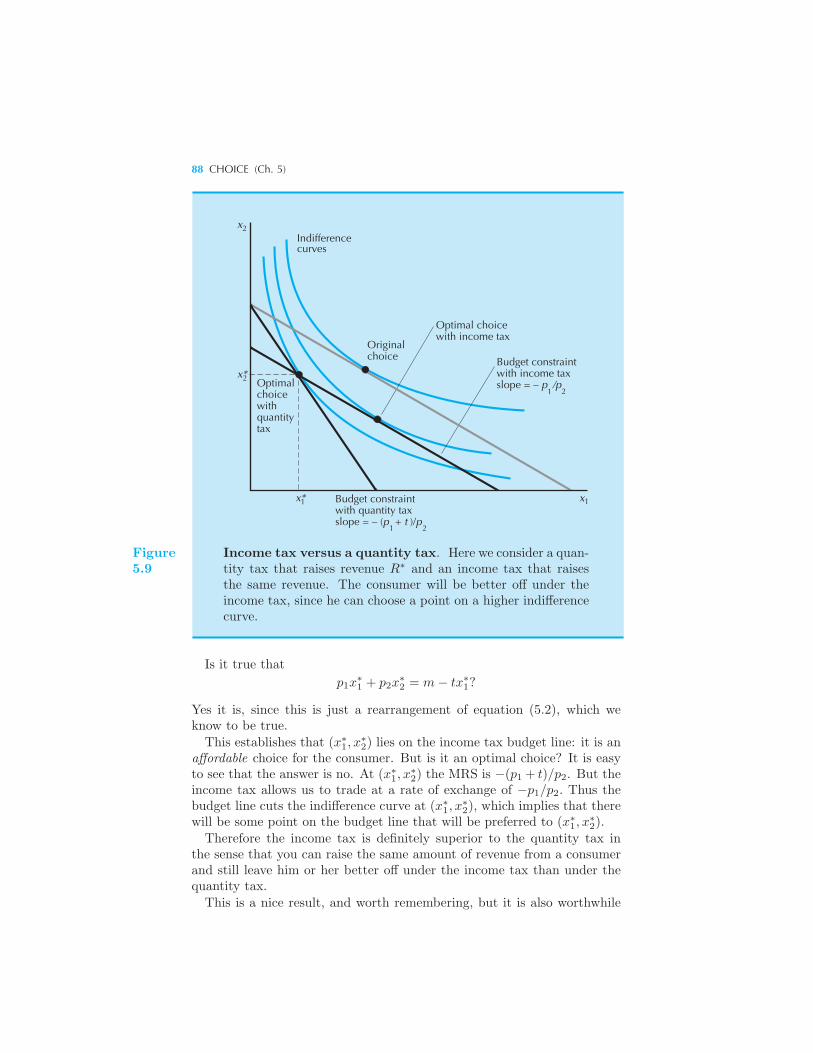
88 CHOICE (Ch. 5)
x
x*
x* x11
2
2Indifferencecurves
Originalchoice
Optimalchoicewithquantitytax
Optimal choicewith income tax
Budget constraintwith income taxslope = – p /p
Budget constraintwith quantity taxslope = – (p + t )/p
1 2
1 2
Figure5.9
Income tax versus a quantity tax. Here we consider a quan-tity tax that raises revenue R∗ and an income tax that raisesthe same revenue. The consumer will be better off under theincome tax, since he can choose a point on a higher indifferencecurve.
Is it true that
p1x∗1 + p2x
∗2 = m− tx∗
1?
Yes it is, since this is just a rearrangement of equation (5.2), which weknow to be true.
This establishes that (x∗1, x
∗2) lies on the income tax budget line: it is an
affordable choice for the consumer. But is it an optimal choice? It is easyto see that the answer is no. At (x∗
1, x∗2) the MRS is −(p1 + t)/p2. But the
income tax allows us to trade at a rate of exchange of −p1/p2. Thus thebudget line cuts the indifference curve at (x∗
1, x∗2), which implies that there
will be some point on the budget line that will be preferred to (x∗1, x
∗2).
Therefore the income tax is definitely superior to the quantity tax inthe sense that you can raise the same amount of revenue from a consumerand still leave him or her better off under the income tax than under thequantity tax.
This is a nice result, and worth remembering, but it is also worthwhile
REVIEW QUESTIONS 89
understanding its limitations. First, it only applies to one consumer. Theargument shows that for any given consumer there is an income tax thatwill raise as much money from that consumer as a quantity tax and leavehim or her better off. But the amount of that income tax will typically differfrom person to person. So a uniform income tax for all consumers is notnecessarily better than a uniform quantity tax for all consumers. (Thinkabout a case where some consumer doesn’t consume any of good 1—thisperson would certainly prefer the quantity tax to a uniform income tax.)
Second, we have assumed that when we impose the tax on income theconsumer’s income doesn’t change. We have assumed that the income taxis basically a lump sum tax—one that just changes the amount of moneya consumer has to spend but doesn’t affect any choices he has to make.This is an unlikely assumption. If income is earned by the consumer, wemight expect that taxing it will discourage earning income, so that after-taxincome might fall by even more than the amount taken by the tax.
Third, we have totally left out the supply response to the tax. We’veshown how demand responds to the tax change, but supply will respondtoo, and a complete analysis would take those changes into account as well.
Summary
1. The optimal choice of the consumer is that bundle in the consumer’sbudget set that lies on the highest indifference curve.
2. Typically the optimal bundle will be characterized by the condition thatthe slope of the indifference curve (the MRS) will equal the slope of thebudget line.
3. If we observe several consumption choices it may be possible to estimatea utility function that would generate that sort of choice behavior. Such autility function can be used to predict future choices and to estimate theutility to consumers of new economic policies.
4. If everyone faces the same prices for the two goods, then everyone willhave the same marginal rate of substitution, and will thus be willing totrade off the two goods in the same way.
REVIEW QUESTIONS
1. If two goods are perfect substitutes, what is the demand function forgood 2?
90 CHOICE (Ch. 5)
2. Suppose that indifference curves are described by straight lines with aslope of −b. Given arbitrary prices and money income p1, p2, and m, whatwill the consumer’s optimal choices look like?
3. Suppose that a consumer always consumes 2 spoons of sugar with eachcup of coffee. If the price of sugar is p1 per spoonful and the price of coffeeis p2 per cup and the consumer has m dollars to spend on coffee and sugar,how much will he or she want to purchase?
4. Suppose that you have highly nonconvex preferences for ice cream andolives, like those given in the text, and that you face prices p1, p2 and havem dollars to spend. List the choices for the optimal consumption bundles.
5. If a consumer has a utility function u(x1, x2) = x1x42, what fraction of
her income will she spend on good 2?
6. For what kind of preferences will the consumer be just as well-off facinga quantity tax as an income tax?
APPENDIX
It is very useful to be able to solve the preference-maximization problem and getalgebraic examples of actual demand functions. We did this in the body of thetext for easy cases like perfect substitutes and perfect complements, and in thisAppendix we’ll see how to do it in more general cases.
First, we will generally want to represent the consumer’s preferences by a utilityfunction, u(x1, x2). We’ve seen in Chapter 4 that this is not a very restrictiveassumption; most well-behaved preferences can be described by a utility function.
The first thing to observe is that we already know how to solve the optimal-choice problem. We just have to put together the facts that we learned in thelast three chapters. We know from this chapter that an optimal choice (x1, x2)must satisfy the condition
MRS(x1, x2) = −p1p2
, (5.3)
and we saw in the Appendix to Chapter 4 that the MRS can be expressed as thenegative of the ratio of derivatives of the utility function. Making this substitutionand cancelling the minus signs, we have
∂u(x1, x2)/∂x1
∂u(x1, x2)/∂x2=
p1p2
. (5.4)
From Chapter 2 we know that the optimal choice must also satisfy the budgetconstraint
p1x1 + p2x2 = m. (5.5)
This gives us two equations—the MRS condition and the budget constraint—and two unknowns, x1 and x2. All we have to do is to solve these two equations
APPENDIX 91
to find the optimal choices of x1 and x2 as a function of the prices and income.There are a number of ways to solve two equations in two unknowns. One waythat always works, although it might not always be the simplest, is to solve thebudget constraint for one of the choices, and then substitute that into the MRScondition.
Rewriting the budget constraint, we have
x2 =m
p2− p1
p2x1 (5.6)
and substituting this into equation (5.4) we get
∂u(x1,m/p2 − (p1/p2)x1)/∂x1
∂u(x1,m/p2 − (p1/p2)x1)/∂x2=
p1p2
.
This rather formidable looking expression has only one unknown variable, x1,and it can typically be solved for x1 in terms of (p1, p2,m). Then the budgetconstraint yields the solution for x2 as a function of prices and income.
We can also derive the solution to the utility maximization problem in a moresystematic way, using calculus conditions for maximization. To do this, we firstpose the utility maximization problem as a constrained maximization problem:
maxx1,x2
u(x1, x2)
such that p1x1 + p2x2 = m.
This problem asks that we choose values of x1 and x2 that do two things:first, they have to satisfy the constraint, and second, they give a larger value foru(x1, x2) than any other values of x1 and x2 that satisfy the constraint.
There are two useful ways to solve this kind of problem. The first way is simplyto solve the constraint for one of the variables in terms of the other and thensubstitute it into the objective function.
For example, for any given value of x1, the amount of x2 that we need tosatisfy the budget constraint is given by the linear function
x2(x1) =m
p2− p1
p2x1. (5.7)
Now substitute x2(x1) for x2 in the utility function to get the unconstrainedmaximization problem
maxx1
u(x1,m/p2 − (p1/p2)x1).
This is an unconstrained maximization problem in x1 alone, since we have usedthe function x2(x1) to ensure that the value of x2 will always satisfy the budgetconstraint, whatever the value of x1 is.
We can solve this kind of problem just by differentiating with respect to x1
and setting the result equal to zero in the usual way. This procedure will give usa first-order condition of the form
∂u(x1, x2(x1))
∂x1+
∂u(x1, x2(x1))
∂x2
dx2
dx1= 0. (5.8)
92 CHOICE (Ch. 5)
Here the first term is the direct effect of how increasing x1 increases utility. Thesecond term consists of two parts: the rate of increase of utility as x2 increases,∂u/∂x2, times dx2/dx1, the rate of increase of x2 as x1 increases in order tocontinue to satisfy the budget equation. We can differentiate (5.7) to calculatethis latter derivative
dx2
dx1= −p1
p2.
Substituting this into (5.8) gives us
∂u(x∗1, x
∗2)/∂x1
∂u(x∗1, x
∗2)/∂x2
=p1p2
,
which just says that the marginal rate of substitution between x1 and x2 mustequal the price ratio at the optimal choice (x∗
1, x∗2). This is exactly the condition
we derived above: the slope of the indifference curve must equal the slope of thebudget line. Of course the optimal choice must also satisfy the budget constraintp1x
∗1 + p2x
∗2 = m, which again gives us two equations in two unknowns.
The second way that these problems can be solved is through the use of La-grange multipliers. This method starts by defining an auxiliary function knownas the Lagrangian:
L = u(x1, x2)− λ(p1x1 + p2x2 −m).
The new variable λ is called a Lagrange multiplier since it is multiplied by theconstraint.3 Then Lagrange’s theorem says that an optimal choice (x∗
1, x∗2) must
satisfy the three first-order conditions
∂L
∂x1=
∂u(x∗1, x
∗2)
∂x1− λp1 = 0
∂L
∂x2=
∂u(x∗1, x
∗2)
∂x2− λp2 = 0
∂L
∂λ= p1x
∗1 + p2x
∗2 −m = 0.
There are several interesting things about these three equations. First, notethat they are simply the derivatives of the Lagrangian with respect to x1, x2,and λ, each set equal to zero. The last derivative, with respect to λ, is just thebudget constraint. Second, we now have three equations for the three unknowns,x1, x2, and λ. We have a hope of solving for x1 and x2 in terms of p1, p2, andm.
Lagrange’s theorem is proved in any advanced calculus book. It is used quiteextensively in advanced economics courses, but for our purposes we only need toknow the statement of the theorem and how to use it.
In our particular case, it is worthwhile noting that if we divide the first condi-tion by the second one, we get
∂u(x∗1, x
∗2)/∂x1
∂u(x∗1, x
∗2)/∂x2
=p1p2
,
which simply says the MRS must equal the price ratio, just as before. The budgetconstraint gives us the other equation, so we are back to two equations in twounknowns.
3 The Greek letter λ is pronounced “lamb-da.”
APPENDIX 93
EXAMPLE: Cobb-Douglas Demand Functions
In Chapter 4 we introduced the Cobb-Douglas utility function
u(x1, x2) = xc1x
d2.
Since utility functions are only defined up to a monotonic transformation, it isconvenient to take logs of this expression and work with
lnu(x1, x2) = c lnx1 + d lnx2.
Let’s find the demand functions for x1 and x2 for the Cobb-Douglas utilityfunction. The problem we want to solve is
maxx1,x2
c lnx1 + d lnx2
such that p1x1 + p2x2 = m.
There are at least three ways to solve this problem. One way is just to writedown the MRS condition and the budget constraint. Using the expression for theMRS derived in Chapter 4, we have
cx2
dx1=
p1p2
p1x1 + p2x2 = m.
These are two equations in two unknowns that can be solved for the optimalchoice of x1 and x2. One way to solve them is to substitute the second into thefirst to get
c(m/p2 − x1p1/p2)
dx1=
p1p2
.
Cross multiplying givesc(m− x1p1) = dp1x1.
Rearranging this equation gives
cm = (c+ d)p1x1
orx1 =
c
c+ d
m
p1.
This is the demand function for x1. To find the demand function for x2, substituteinto the budget constraint to get
x2 =m
p2− p1
p2
c
c+ d
m
p1
=d
c+ d
m
p2.
94 CHOICE (Ch. 5)
The second way is to substitute the budget constraint into the maximizationproblem at the beginning. If we do this, our problem becomes
maxx1
c lnx1 + d ln(m/p2 − x1p1/p2).
The first-order condition for this problem is
c
x1− d
p2m− p1x1
p1p2
= 0.
A little algebra—which you should do!—gives us the solution
x1 =c
c+ d
m
p1.
Substitute this back into the budget constraint x2 = m/p2 − x1p1/p2 to get
x2 =d
c+ d
m
p2.
These are the demand functions for the two goods, which, happily, are the sameas those derived earlier by the other method.
Now for Lagrange’s method. Set up the Lagrangian
L = c lnx1 + d lnx2 − λ(p1x1 + p2x2 −m)
and differentiate to get the three first-order conditions
∂L
∂x1=
c
x1− λp1 = 0
∂L
∂x2=
d
x2− λp2 = 0
∂L
∂λ= p1x1 + p2x2 −m = 0.
Now the trick is to solve them! The best way to proceed is to first solve for λ andthen for x1 and x2. So we rearrange and cross multiply the first two equationsto get
c = λp1x1
d = λp2x2.
These equations are just asking to be added together:
c+ d = λ(p1x1 + p2x2) = λm,
which gives us
λ =c+ d
m.
Substitute this back into the first two equations and solve for x1 and x2 to get
x1 =c
c+ d
m
p1
x2 =d
c+ d
m
p2,
just as before.
CHAPTER 6
DEMAND
In the last chapter we presented the basic model of consumer choice: howmaximizing utility subject to a budget constraint yields optimal choices.We saw that the optimal choices of the consumer depend on the consumer’sincome and the prices of the goods, and we worked a few examples to seewhat the optimal choices are for some simple kinds of preferences.The consumer’s demand functions give the optimal amounts of each
of the goods as a function of the prices and income faced by the consumer.We write the demand functions as
x1 = x1(p1, p2,m)
x2 = x2(p1, p2,m).
The left-hand side of each equation stands for the quantity demanded. Theright-hand side of each equation is the function that relates the prices andincome to that quantity.In this chapter we will examine how the demand for a good changes as
prices and income change. Studying how a choice responds to changes in theeconomic environment is known as comparative statics, which we firstdescribed in Chapter 1. “Comparative” means that we want to compare
96 DEMAND (Ch. 6)
two situations: before and after the change in the economic environment.“Statics” means that we are not concerned with any adjustment processthat may be involved in moving from one choice to another; rather we willonly examine the equilibrium choice.In the case of the consumer, there are only two things in our model
that affect the optimal choice: prices and income. The comparative staticsquestions in consumer theory therefore involve investigating how demandchanges when prices and income change.
6.1 Normal and Inferior Goods
We start by considering how a consumer’s demand for a good changesas his income changes. We want to know how the optimal choice at oneincome compares to the optimal choice at another level of income. Duringthis exercise, we will hold the prices fixed and examine only the change indemand due to the income change.We know how an increase in money income affects the budget line when
prices are fixed—it shifts it outward in a parallel fashion. So how does thisaffect demand?We would normally think that the demand for each good would increase
when income increases, as shown in Figure 6.1. Economists, with a singularlack of imagination, call such goods normal goods. If good 1 is a normalgood, then the demand for it increases when income increases, and de-creases when income decreases. For a normal good the quantity demandedalways changes in the same way as income changes:
Δx1
Δm> 0.
If something is called normal, you can be sure that there must be apossibility of being abnormal. And indeed there is. Figure 6.2 presentsan example of nice, well-behaved indifference curves where an increase ofincome results in a reduction in the consumption of one of the goods. Sucha good is called an inferior good. This may be “abnormal,” but whenyou think about it, inferior goods aren’t all that unusual. There are manygoods for which demand decreases as income increases; examples mightinclude gruel, bologna, shacks, or nearly any kind of low-quality good.Whether a good is inferior or not depends on the income level that we
are examining. It might very well be that very poor people consume morebologna as their income increases. But after a point, the consumption ofbologna would probably decline as income continued to increase. Since inreal life the consumption of goods can increase or decrease when incomeincreases, it is comforting to know that economic theory allows for bothpossibilities.
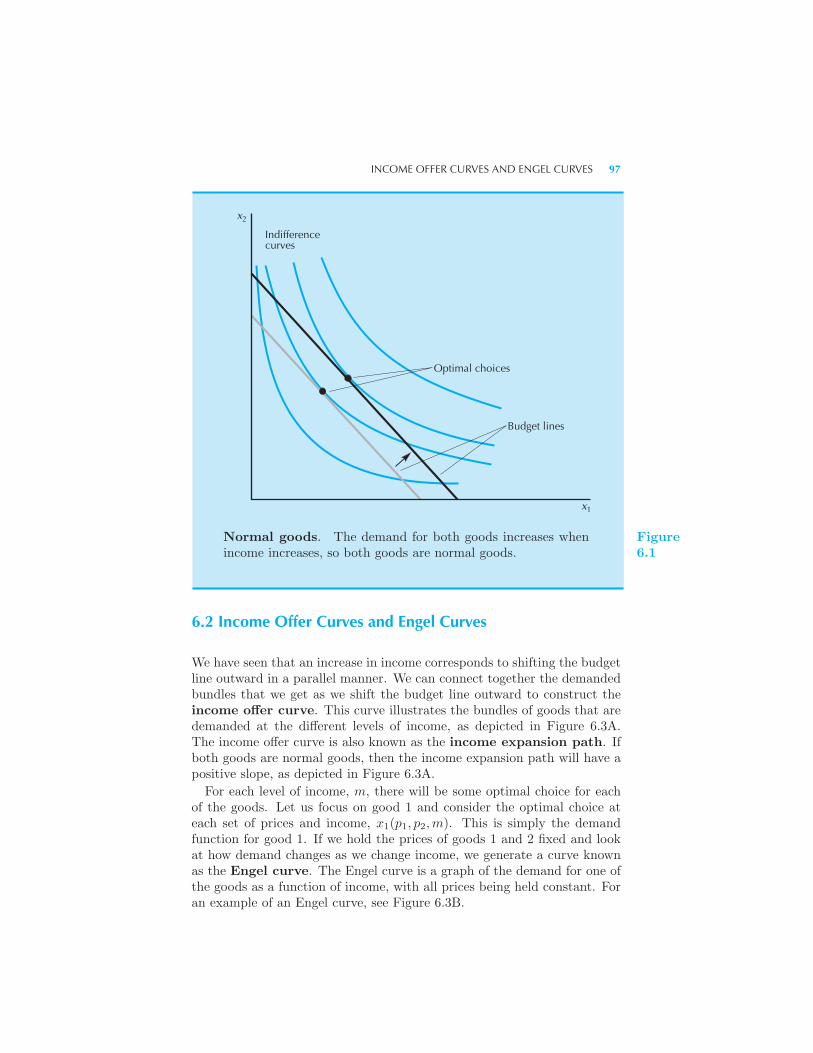
INCOME OFFER CURVES AND ENGEL CURVES 97
Indifferencecurves
Optimal choices
Budget lines
x1
x2
Normal goods. The demand for both goods increases whenincome increases, so both goods are normal goods.
Figure6.1
6.2 Income Offer Curves and Engel Curves
We have seen that an increase in income corresponds to shifting the budgetline outward in a parallel manner. We can connect together the demandedbundles that we get as we shift the budget line outward to construct theincome offer curve. This curve illustrates the bundles of goods that aredemanded at the different levels of income, as depicted in Figure 6.3A.The income offer curve is also known as the income expansion path. Ifboth goods are normal goods, then the income expansion path will have apositive slope, as depicted in Figure 6.3A.
For each level of income, m, there will be some optimal choice for eachof the goods. Let us focus on good 1 and consider the optimal choice ateach set of prices and income, x1(p1, p2,m). This is simply the demandfunction for good 1. If we hold the prices of goods 1 and 2 fixed and lookat how demand changes as we change income, we generate a curve knownas the Engel curve. The Engel curve is a graph of the demand for one ofthe goods as a function of income, with all prices being held constant. Foran example of an Engel curve, see Figure 6.3B.
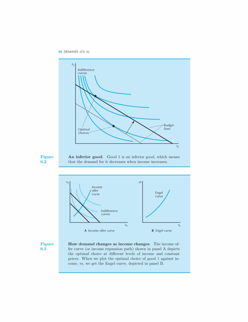
98 DEMAND (Ch. 6)
Indifferencecurves
x2
Optimalchoices
Budgetlines
x1
Figure6.2
An inferior good. Good 1 is an inferior good, which meansthat the demand for it decreases when income increases.
Incomeoffercurve
Indifferencecurves
Engelcurve
m
xx
x2
1 1
A Income offer curve B Engel curve
Figure6.3
How demand changes as income changes. The income of-fer curve (or income expansion path) shown in panel A depictsthe optimal choice at different levels of income and constantprices. When we plot the optimal choice of good 1 against in-come, m, we get the Engel curve, depicted in panel B.
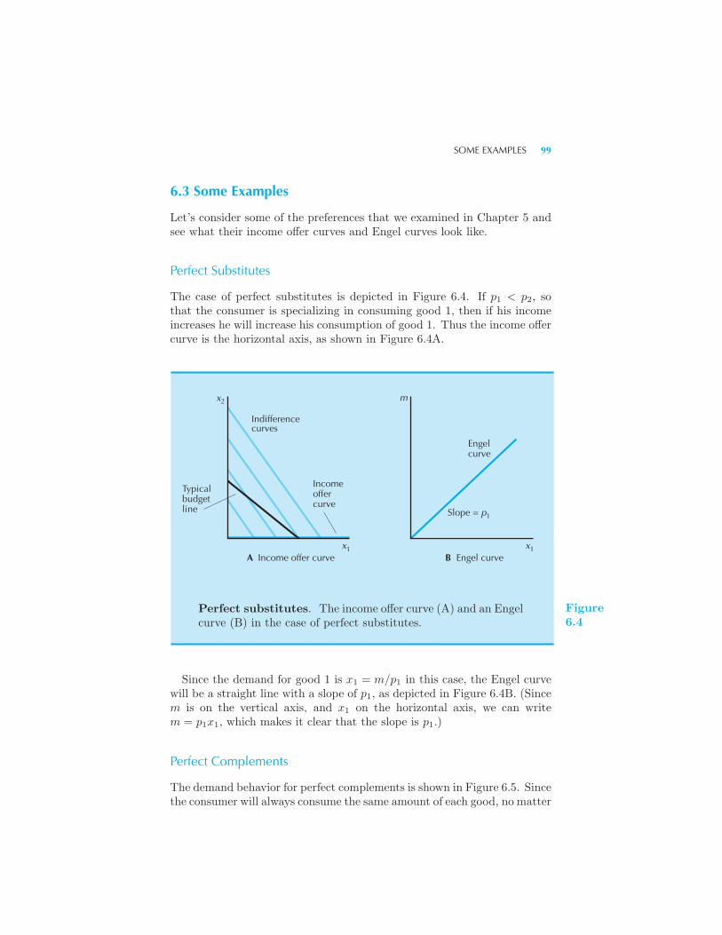
SOME EXAMPLES 99
6.3 Some Examples
Let’s consider some of the preferences that we examined in Chapter 5 andsee what their income offer curves and Engel curves look like.
Perfect Substitutes
The case of perfect substitutes is depicted in Figure 6.4. If p1 < p2, sothat the consumer is specializing in consuming good 1, then if his incomeincreases he will increase his consumption of good 1. Thus the income offercurve is the horizontal axis, as shown in Figure 6.4A.
Indifferencecurves
Incomeoffercurve
Typicalbudgetline
Engelcurve
Slope = p1
11
2x m
x xA Income offer curve B Engel curve
Perfect substitutes. The income offer curve (A) and an Engelcurve (B) in the case of perfect substitutes.
Figure6.4
Since the demand for good 1 is x1 = m/p1 in this case, the Engel curvewill be a straight line with a slope of p1, as depicted in Figure 6.4B. (Sincem is on the vertical axis, and x1 on the horizontal axis, we can writem = p1x1, which makes it clear that the slope is p1.)
Perfect Complements
The demand behavior for perfect complements is shown in Figure 6.5. Sincethe consumer will always consume the same amount of each good, no matter
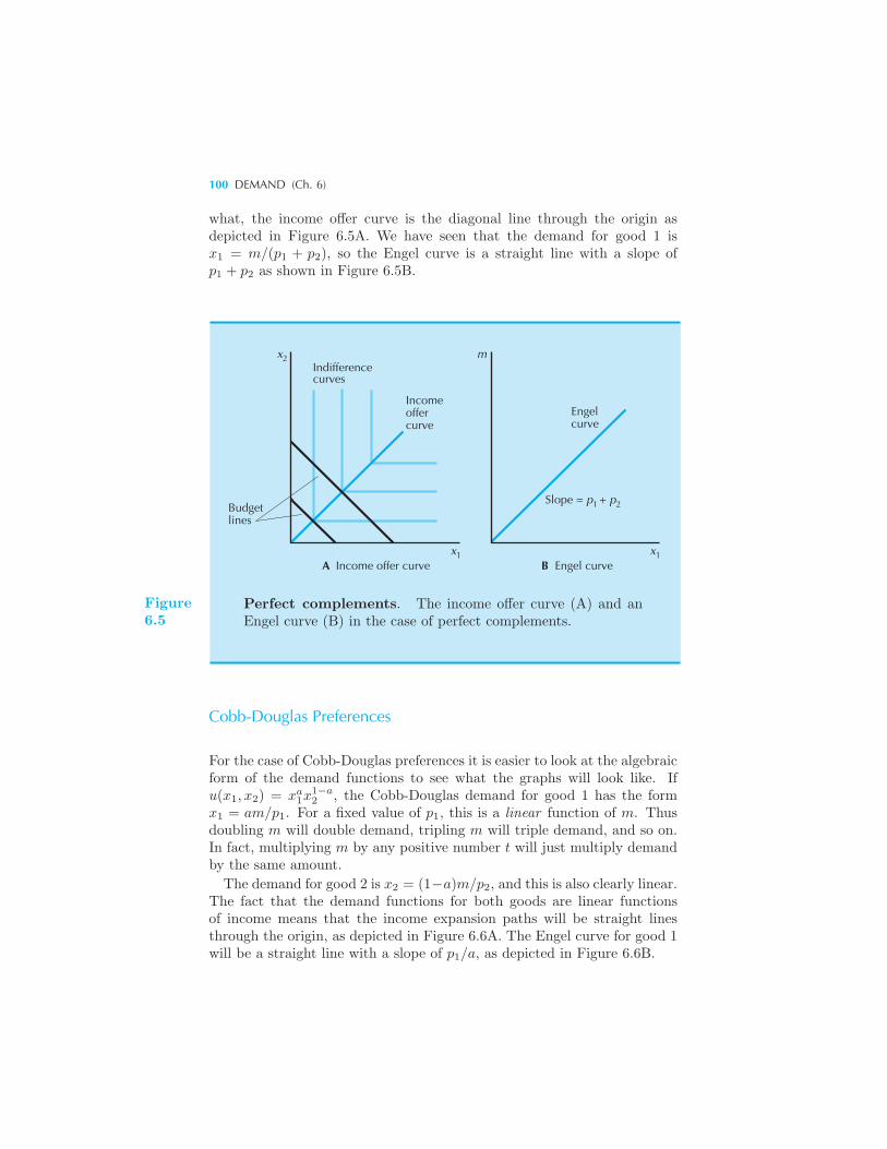
100 DEMAND (Ch. 6)
what, the income offer curve is the diagonal line through the origin asdepicted in Figure 6.5A. We have seen that the demand for good 1 isx1 = m/(p1 + p2), so the Engel curve is a straight line with a slope ofp1 + p2 as shown in Figure 6.5B.
Indifferencecurves
Income offercurve
Budgetlines
Engelcurve
Slope = p + p
mx
x x
2
1 2
11A Income offer curve B Engel curve
Figure6.5
Perfect complements. The income offer curve (A) and anEngel curve (B) in the case of perfect complements.
Cobb-Douglas Preferences
For the case of Cobb-Douglas preferences it is easier to look at the algebraicform of the demand functions to see what the graphs will look like. Ifu(x1, x2) = xa
1x1−a2 , the Cobb-Douglas demand for good 1 has the form
x1 = am/p1. For a fixed value of p1, this is a linear function of m. Thusdoubling m will double demand, tripling m will triple demand, and so on.In fact, multiplying m by any positive number t will just multiply demandby the same amount.
The demand for good 2 is x2 = (1−a)m/p2, and this is also clearly linear.The fact that the demand functions for both goods are linear functionsof income means that the income expansion paths will be straight linesthrough the origin, as depicted in Figure 6.6A. The Engel curve for good 1will be a straight line with a slope of p1/a, as depicted in Figure 6.6B.
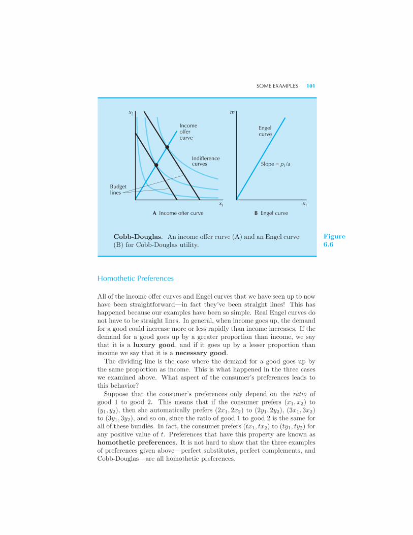
SOME EXAMPLES 101
Income offercurve
Indifferencecurves
Budgetlines
Engelcurve
x m
x x1 1
1
2
Slope = p /a
B Engel curveA Income offer curve
Cobb-Douglas. An income offer curve (A) and an Engel curve(B) for Cobb-Douglas utility.
Figure6.6
Homothetic Preferences
All of the income offer curves and Engel curves that we have seen up to nowhave been straightforward—in fact they’ve been straight lines! This hashappened because our examples have been so simple. Real Engel curves donot have to be straight lines. In general, when income goes up, the demandfor a good could increase more or less rapidly than income increases. If thedemand for a good goes up by a greater proportion than income, we saythat it is a luxury good, and if it goes up by a lesser proportion thanincome we say that it is a necessary good.The dividing line is the case where the demand for a good goes up by
the same proportion as income. This is what happened in the three caseswe examined above. What aspect of the consumer’s preferences leads tothis behavior?Suppose that the consumer’s preferences only depend on the ratio of
good 1 to good 2. This means that if the consumer prefers (x1, x2) to(y1, y2), then she automatically prefers (2x1, 2x2) to (2y1, 2y2), (3x1, 3x2)to (3y1, 3y2), and so on, since the ratio of good 1 to good 2 is the same forall of these bundles. In fact, the consumer prefers (tx1, tx2) to (ty1, ty2) forany positive value of t. Preferences that have this property are known ashomothetic preferences. It is not hard to show that the three examplesof preferences given above—perfect substitutes, perfect complements, andCobb-Douglas—are all homothetic preferences.
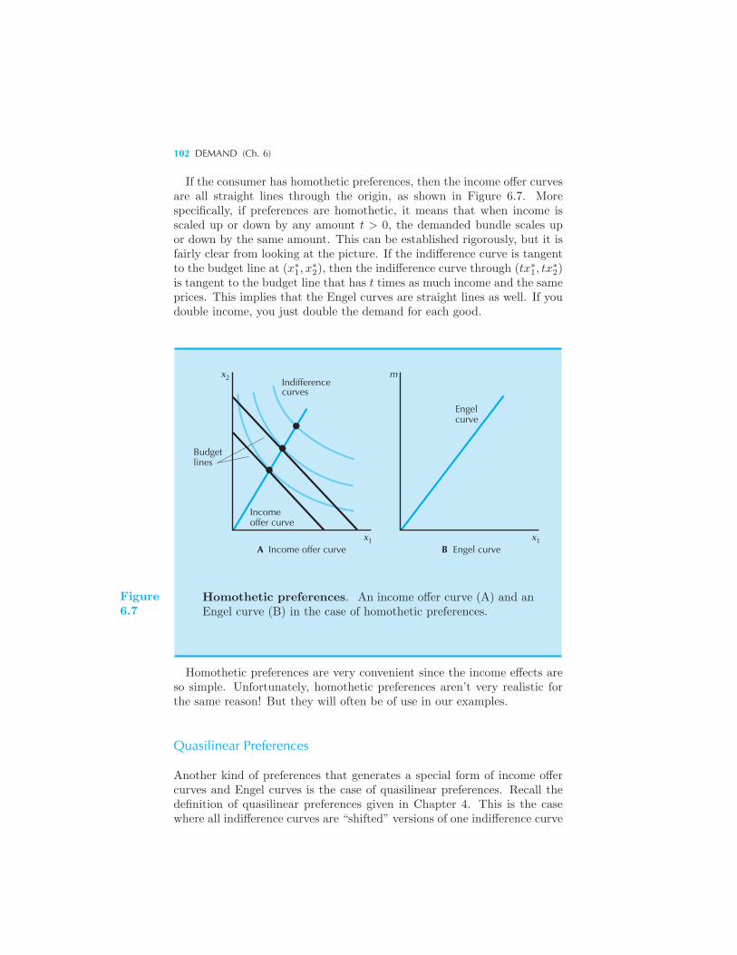
102 DEMAND (Ch. 6)
If the consumer has homothetic preferences, then the income offer curvesare all straight lines through the origin, as shown in Figure 6.7. Morespecifically, if preferences are homothetic, it means that when income isscaled up or down by any amount t > 0, the demanded bundle scales upor down by the same amount. This can be established rigorously, but it isfairly clear from looking at the picture. If the indifference curve is tangentto the budget line at (x∗
1, x∗2), then the indifference curve through (tx∗
1, tx∗2)
is tangent to the budget line that has t times as much income and the sameprices. This implies that the Engel curves are straight lines as well. If youdouble income, you just double the demand for each good.
x
x x
m2
1 1
Indifferencecurves
Budgetlines
Incomeoffer curve
Engelcurve
A Income offer curve B Engel curve
Figure6.7
Homothetic preferences. An income offer curve (A) and anEngel curve (B) in the case of homothetic preferences.
Homothetic preferences are very convenient since the income effects areso simple. Unfortunately, homothetic preferences aren’t very realistic forthe same reason! But they will often be of use in our examples.
Quasilinear Preferences
Another kind of preferences that generates a special form of income offercurves and Engel curves is the case of quasilinear preferences. Recall thedefinition of quasilinear preferences given in Chapter 4. This is the casewhere all indifference curves are “shifted” versions of one indifference curve
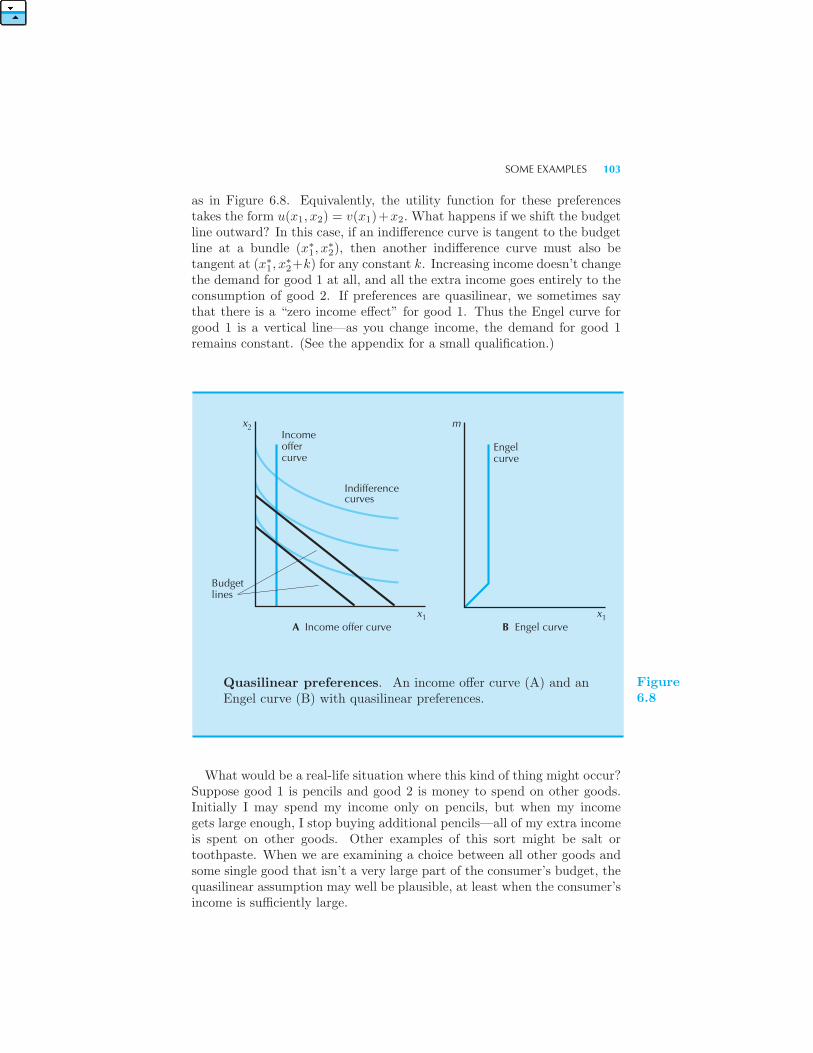
SOME EXAMPLES 103
as in Figure 6.8. Equivalently, the utility function for these preferencestakes the form u(x1, x2) = v(x1)+x2. What happens if we shift the budgetline outward? In this case, if an indifference curve is tangent to the budgetline at a bundle (x∗
1, x∗2), then another indifference curve must also be
tangent at (x∗1, x
∗2+k) for any constant k. Increasing income doesn’t change
the demand for good 1 at all, and all the extra income goes entirely to theconsumption of good 2. If preferences are quasilinear, we sometimes saythat there is a “zero income effect” for good 1. Thus the Engel curve forgood 1 is a vertical line—as you change income, the demand for good 1remains constant. (See the appendix for a small qualification.)
mx
x x1 1
2Incomeoffercurve
Indifferencecurves
Engelcurve
Budgetlines
A Income offer curve B Engel curve
Quasilinear preferences. An income offer curve (A) and anEngel curve (B) with quasilinear preferences.
Figure6.8
What would be a real-life situation where this kind of thing might occur?Suppose good 1 is pencils and good 2 is money to spend on other goods.Initially I may spend my income only on pencils, but when my incomegets large enough, I stop buying additional pencils—all of my extra incomeis spent on other goods. Other examples of this sort might be salt ortoothpaste. When we are examining a choice between all other goods andsome single good that isn’t a very large part of the consumer’s budget, thequasilinear assumption may well be plausible, at least when the consumer’sincome is sufficiently large.
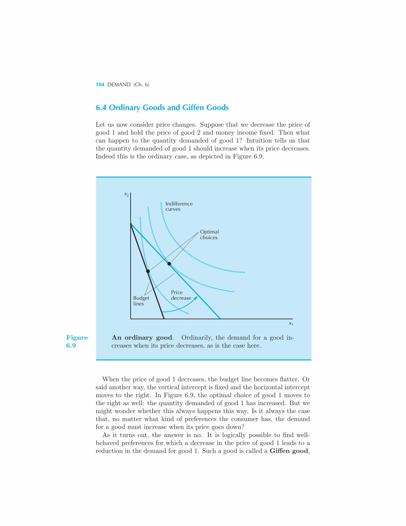
104 DEMAND (Ch. 6)
6.4 Ordinary Goods and Giffen Goods
Let us now consider price changes. Suppose that we decrease the price ofgood 1 and hold the price of good 2 and money income fixed. Then whatcan happen to the quantity demanded of good 1? Intuition tells us thatthe quantity demanded of good 1 should increase when its price decreases.Indeed this is the ordinary case, as depicted in Figure 6.9.
x1
PricedecreaseBudget
lines
Indifferencecurves
Optimalchoices
x2
Figure6.9
An ordinary good. Ordinarily, the demand for a good in-creases when its price decreases, as is the case here.
When the price of good 1 decreases, the budget line becomes flatter. Orsaid another way, the vertical intercept is fixed and the horizontal interceptmoves to the right. In Figure 6.9, the optimal choice of good 1 moves tothe right as well: the quantity demanded of good 1 has increased. But wemight wonder whether this always happens this way. Is it always the casethat, no matter what kind of preferences the consumer has, the demandfor a good must increase when its price goes down?As it turns out, the answer is no. It is logically possible to find well-
behaved preferences for which a decrease in the price of good 1 leads to areduction in the demand for good 1. Such a good is called a Giffen good,
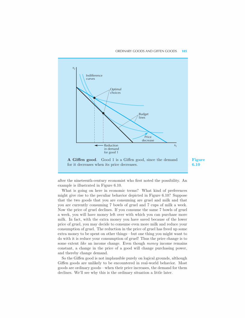
ORDINARY GOODS AND GIFFEN GOODS 105
Reduction in demandfor good 1
Budgetlines
Pricedecrease
Optimalchoices
Indifferencecurves
x2
1x
A Giffen good. Good 1 is a Giffen good, since the demandfor it decreases when its price decreases.
Figure6.10
after the nineteenth-century economist who first noted the possibility. Anexample is illustrated in Figure 6.10.
What is going on here in economic terms? What kind of preferencesmight give rise to the peculiar behavior depicted in Figure 6.10? Supposethat the two goods that you are consuming are gruel and milk and thatyou are currently consuming 7 bowls of gruel and 7 cups of milk a week.Now the price of gruel declines. If you consume the same 7 bowls of gruela week, you will have money left over with which you can purchase moremilk. In fact, with the extra money you have saved because of the lowerprice of gruel, you may decide to consume even more milk and reduce yourconsumption of gruel. The reduction in the price of gruel has freed up someextra money to be spent on other things—but one thing you might want todo with it is reduce your consumption of gruel! Thus the price change is tosome extent like an income change. Even though money income remainsconstant, a change in the price of a good will change purchasing power,and thereby change demand.
So the Giffen good is not implausible purely on logical grounds, althoughGiffen goods are unlikely to be encountered in real-world behavior. Mostgoods are ordinary goods—when their price increases, the demand for themdeclines. We’ll see why this is the ordinary situation a little later.
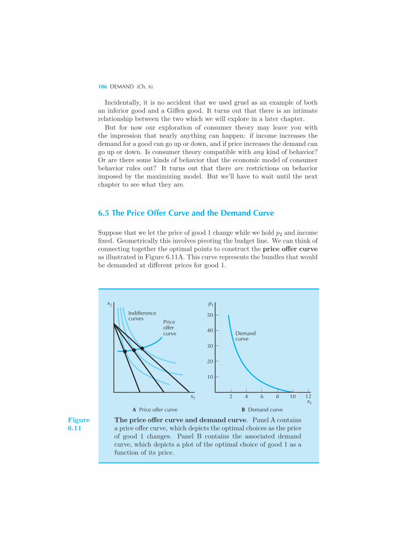
106 DEMAND (Ch. 6)
Incidentally, it is no accident that we used gruel as an example of bothan inferior good and a Giffen good. It turns out that there is an intimaterelationship between the two which we will explore in a later chapter.
But for now our exploration of consumer theory may leave you withthe impression that nearly anything can happen: if income increases thedemand for a good can go up or down, and if price increases the demand cango up or down. Is consumer theory compatible with any kind of behavior?Or are there some kinds of behavior that the economic model of consumerbehavior rules out? It turns out that there are restrictions on behaviorimposed by the maximizing model. But we’ll have to wait until the nextchapter to see what they are.
6.5 The Price Offer Curve and the Demand Curve
Suppose that we let the price of good 1 change while we hold p2 and incomefixed. Geometrically this involves pivoting the budget line. We can think ofconnecting together the optimal points to construct the price offer curveas illustrated in Figure 6.11A. This curve represents the bundles that wouldbe demanded at different prices for good 1.
x p
xx
2 1
11
Indifferencecurves
Priceoffercurve Demand
curve
A Price offer curve B Demand curve
2 4 6 8 10 12
50
40
30
20
10
Figure6.11
The price offer curve and demand curve. Panel A containsa price offer curve, which depicts the optimal choices as the priceof good 1 changes. Panel B contains the associated demandcurve, which depicts a plot of the optimal choice of good 1 as afunction of its price.
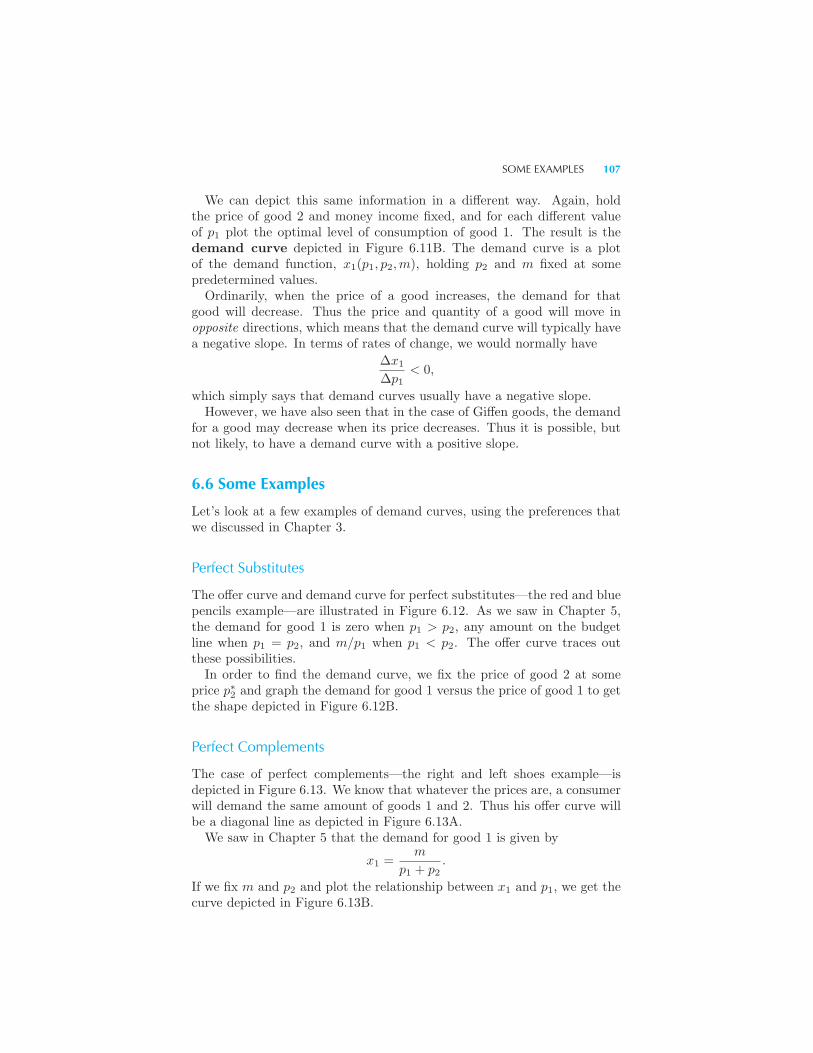
SOME EXAMPLES 107
We can depict this same information in a different way. Again, holdthe price of good 2 and money income fixed, and for each different valueof p1 plot the optimal level of consumption of good 1. The result is thedemand curve depicted in Figure 6.11B. The demand curve is a plotof the demand function, x1(p1, p2,m), holding p2 and m fixed at somepredetermined values.Ordinarily, when the price of a good increases, the demand for that
good will decrease. Thus the price and quantity of a good will move inopposite directions, which means that the demand curve will typically havea negative slope. In terms of rates of change, we would normally have
Δx1
Δp1< 0,
which simply says that demand curves usually have a negative slope.However, we have also seen that in the case of Giffen goods, the demand
for a good may decrease when its price decreases. Thus it is possible, butnot likely, to have a demand curve with a positive slope.
6.6 Some Examples
Let’s look at a few examples of demand curves, using the preferences thatwe discussed in Chapter 3.
Perfect Substitutes
The offer curve and demand curve for perfect substitutes—the red and bluepencils example—are illustrated in Figure 6.12. As we saw in Chapter 5,the demand for good 1 is zero when p1 > p2, any amount on the budgetline when p1 = p2, and m/p1 when p1 < p2. The offer curve traces outthese possibilities.In order to find the demand curve, we fix the price of good 2 at some
price p∗2 and graph the demand for good 1 versus the price of good 1 to getthe shape depicted in Figure 6.12B.
Perfect Complements
The case of perfect complements—the right and left shoes example—isdepicted in Figure 6.13. We know that whatever the prices are, a consumerwill demand the same amount of goods 1 and 2. Thus his offer curve willbe a diagonal line as depicted in Figure 6.13A.We saw in Chapter 5 that the demand for good 1 is given by
x1 =m
p1 + p2.
If we fix m and p2 and plot the relationship between x1 and p1, we get thecurve depicted in Figure 6.13B.
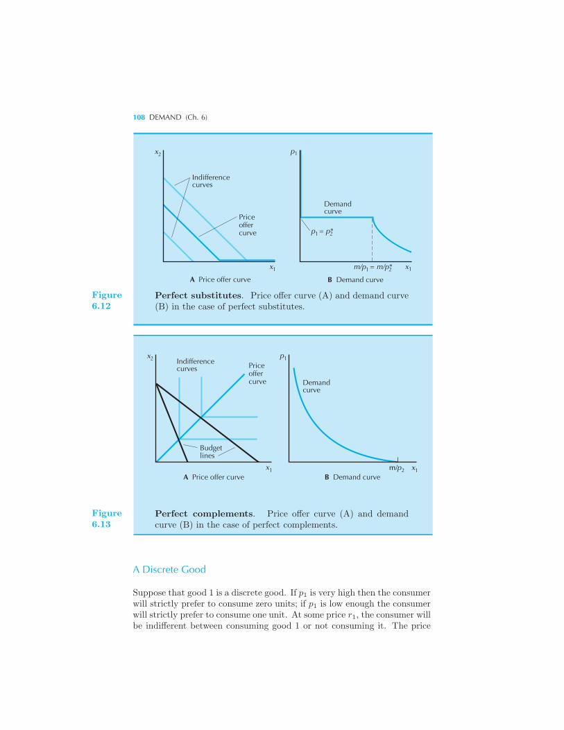
108 DEMAND (Ch. 6)
x
Indifferencecurves
Priceoffercurve
x
A Price offer curve1
2 1
1 2
1 2 1
B Demand curve
x
p = p*
p
m/p = m/p*
Demand curve
Figure6.12
Perfect substitutes. Price offer curve (A) and demand curve(B) in the case of perfect substitutes.
x p
x xpm/
2 1
1 12
Indifferencecurves Price
offercurve Demand
curve
Budgetlines
A Price offer curve B Demand curve
Figure6.13
Perfect complements. Price offer curve (A) and demandcurve (B) in the case of perfect complements.
A Discrete Good
Suppose that good 1 is a discrete good. If p1 is very high then the consumerwill strictly prefer to consume zero units; if p1 is low enough the consumerwill strictly prefer to consume one unit. At some price r1, the consumer willbe indifferent between consuming good 1 or not consuming it. The price
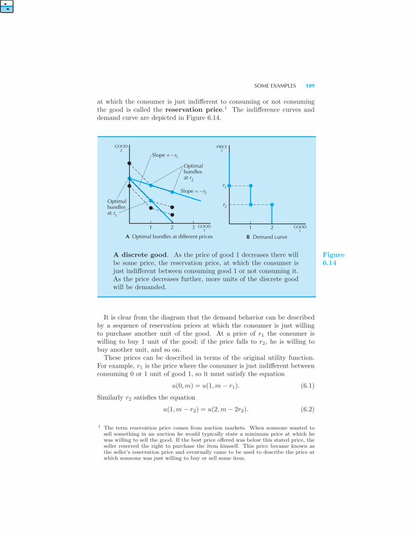
SOME EXAMPLES 109
at which the consumer is just indifferent to consuming or not consumingthe good is called the reservation price.1 The indifference curves anddemand curve are depicted in Figure 6.14.
PRICE1
GOOD1
B Demand curve
1 2
GOOD2
GOOD1
A Optimal bundles at different prices
1 2 3
Slope = –r
Slope = –r
Optimalbundlesat r
Optimalbundlesat r
r
r
1
2
1
2
1
2
A discrete good. As the price of good 1 decreases there willbe some price, the reservation price, at which the consumer isjust indifferent between consuming good 1 or not consuming it.As the price decreases further, more units of the discrete goodwill be demanded.
Figure6.14
It is clear from the diagram that the demand behavior can be describedby a sequence of reservation prices at which the consumer is just willingto purchase another unit of the good. At a price of r1 the consumer iswilling to buy 1 unit of the good; if the price falls to r2, he is willing tobuy another unit, and so on.These prices can be described in terms of the original utility function.
For example, r1 is the price where the consumer is just indifferent betweenconsuming 0 or 1 unit of good 1, so it must satisfy the equation
u(0,m) = u(1,m− r1). (6.1)
Similarly r2 satisfies the equation
u(1,m− r2) = u(2,m− 2r2). (6.2)
1 The term reservation price comes from auction markets. When someone wanted tosell something in an auction he would typically state a minimum price at which hewas willing to sell the good. If the best price offered was below this stated price, theseller reserved the right to purchase the item himself. This price became known asthe seller’s reservation price and eventually came to be used to describe the price atwhich someone was just willing to buy or sell some item.
110 DEMAND (Ch. 6)
The left-hand side of this equation is the utility from consuming one unit ofthe good at a price of r2. The right-hand side is the utility from consumingtwo units of the good, each of which sells for r2.
If the utility function is quasilinear, then the formulas describing thereservation prices become somewhat simpler. If u(x1, x2) = v(x1) + x2,and v(0) = 0, then we can write equation (6.1) as
v(0) +m = m = v(1) +m− r1.
Since v(0) = 0, we can solve for r1 to find
r1 = v(1). (6.3)
Similarly, we can write equation (6.2) as
v(1) +m− r2 = v(2) +m− 2r2.
Canceling terms and rearranging, this expression becomes
r2 = v(2)− v(1).
Proceeding in this manner, the reservation price for the third unit of con-sumption is given by
r3 = v(3)− v(2)
and so on.In each case, the reservation price measures the increment in utility nec-
essary to induce the consumer to choose an additional unit of the good.Loosely speaking, the reservation prices measure the marginal utilities as-sociated with different levels of consumption of good 1. Our assumptionof convex preferences implies that the sequence of reservation prices mustdecrease: r1 > r2 > r3 · · ·.Because of the special structure of the quasilinear utility function, the
reservation prices do not depend on the amount of good 2 that the consumerhas. This is certainly a special case, but it makes it very easy to describedemand behavior. Given any price p, we just find where it falls in the listof reservation prices. Suppose that p falls between r6 and r7, for example.The fact that r6 > p means that the consumer is willing to give up p dollarsper unit bought to get 6 units of good 1, and the fact that p > r7 meansthat the consumer is not willing to give up p dollars per unit to get theseventh unit of good 1.This argument is quite intuitive, but let’s look at the math just to make
sure that it is clear. Suppose that the consumer demands 6 units of good 1.We want to show that we must have r6 ≥ p ≥ r7.If the consumer is maximizing utility, then we must have
v(6) +m− 6p ≥ v(x1) +m− px1
SUBSTITUTES AND COMPLEMENTS 111
for all possible choices of x1. In particular, we must have that
v(6) +m− 6p ≥ v(5) +m− 5p.
Rearranging this equation we have
r6 = v(6)− v(5) ≥ p,
which is half of what we wanted to show.By the same logic,
v(6) +m− 6p ≥ v(7) +m− 7p.
Rearranging this gives us
p ≥ v(7)− v(6) = r7,
which is the other half of the inequality we wanted to establish.
6.7 Substitutes and Complements
We have already used the terms substitutes and complements, but it is nowappropriate to give a formal definition. Since we have seen perfect substi-tutes and perfect complements several times already, it seems reasonableto look at the imperfect case.Let’s think about substitutes first. We said that red pencils and blue
pencils might be thought of as perfect substitutes, at least for someone whodidn’t care about color. But what about pencils and pens? This is a caseof “imperfect” substitutes. That is, pens and pencils are, to some degree,a substitute for each other, although they aren’t as perfect a substitute foreach other as red pencils and blue pencils.Similarly, we said that right shoes and left shoes were perfect comple-
ments. But what about a pair of shoes and a pair of socks? Right shoesand left shoes are nearly always consumed together, and shoes and socksare usually consumed together. Complementary goods are those like shoesand socks that tend to be consumed together, albeit not always.Now that we’ve discussed the basic idea of complements and substitutes,
we can give a precise economic definition. Recall that the demand functionfor good 1, say, will typically be a function of the price of both good 1 andgood 2, so we write x1(p1, p2,m). We can ask how the demand for good 1changes as the price of good 2 changes: does it go up or down?If the demand for good 1 goes up when the price of good 2 goes up, then
we say that good 1 is a substitute for good 2. In terms of rates of change,good 1 is a substitute for good 2 if
Δx1
Δp2> 0.
112 DEMAND (Ch. 6)
The idea is that when good 2 gets more expensive the consumer switches toconsuming good 1: the consumer substitutes away from the more expensivegood to the less expensive good.On the other hand, if the demand for good 1 goes down when the price
of good 2 goes up, we say that good 1 is a complement to good 2. Thismeans that
Δx1
Δp2< 0.
Complements are goods that are consumed together, like coffee and sugar,so when the price of one good rises, the consumption of both goods willtend to decrease.The cases of perfect substitutes and perfect complements illustrate these
points nicely. Note that Δx1/Δp2 is positive (or zero) in the case of perfectsubstitutes, and that Δx1/Δp2 is negative in the case of perfect comple-ments.A couple of warnings are in order about these concepts. First, the two-
good case is rather special when it comes to complements and substitutes.Since income is being held fixed, if you spend more money on good 1, you’llhave to spend less on good 2. This puts some restrictions on the kinds ofbehavior that are possible. When there are more than two goods, theserestrictions are not so much of a problem.Second, although the definition of substitutes and complements in terms
of consumer demand behavior seems sensible, there are some difficultieswith the definitions in more general environments. For example, if we usethe above definitions in a situation involving more than two goods, it isperfectly possible that good 1 may be a substitute for good 3, but good 3may be a complement for good 1. Because of this peculiar feature, moreadvanced treatments typically use a somewhat different definition of sub-stitutes and complements. The definitions given above describe conceptsknown as gross substitutes and gross complements; they will be suf-ficient for our needs.
6.8 The Inverse Demand Function
If we hold p2 and m fixed and plot p1 against x1 we get the demandcurve. As suggested above, we typically think that the demand curveslopes downwards, so that higher prices lead to less demand, although theGiffen example shows that it could be otherwise.As long as we do have a downward-sloping demand curve, as is usual,
it is meaningful to speak of the inverse demand function. The inversedemand function is the demand function viewing price as a function ofquantity. That is, for each level of demand for good 1, the inverse demandfunction measures what the price of good 1 would have to be in order forthe consumer to choose that level of consumption. So the inverse demand
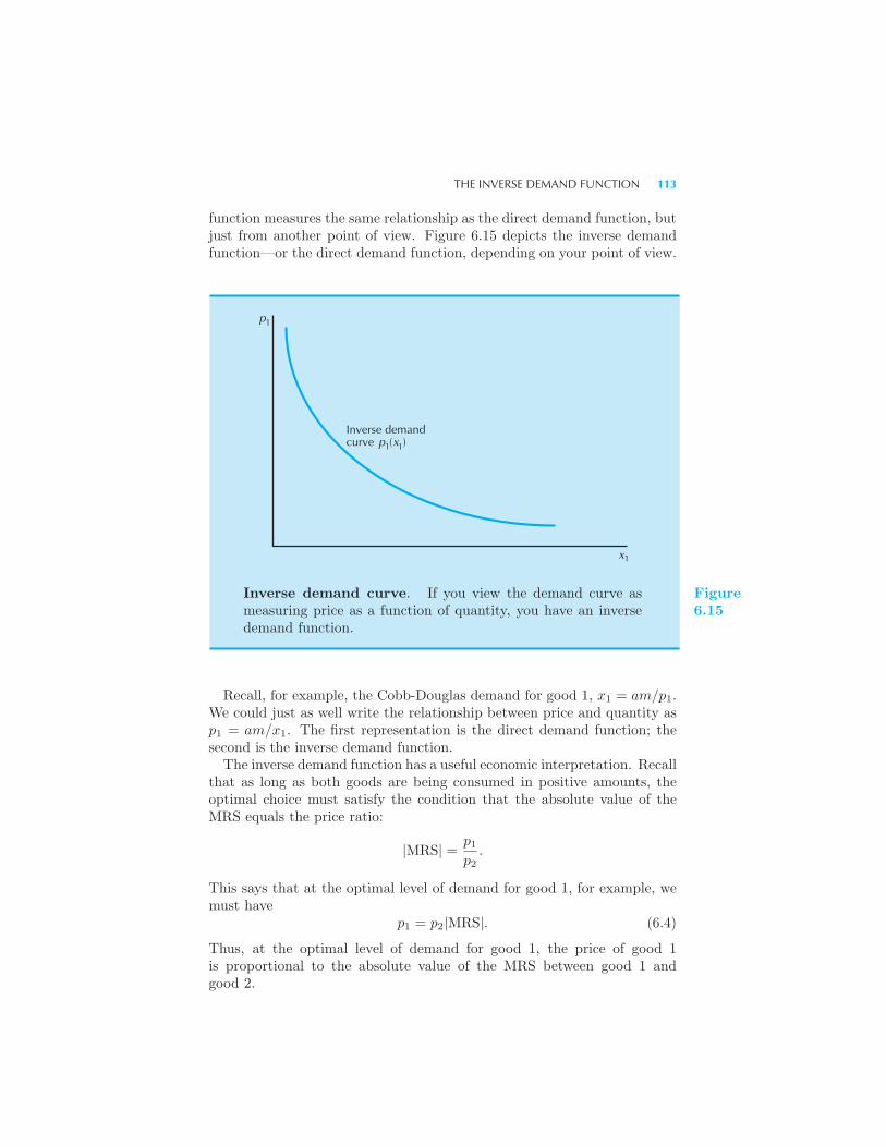
THE INVERSE DEMAND FUNCTION 113
function measures the same relationship as the direct demand function, butjust from another point of view. Figure 6.15 depicts the inverse demandfunction—or the direct demand function, depending on your point of view.
Inverse demandcurve p (x )1 1
p1
x1
Inverse demand curve. If you view the demand curve asmeasuring price as a function of quantity, you have an inversedemand function.
Figure6.15
Recall, for example, the Cobb-Douglas demand for good 1, x1 = am/p1.We could just as well write the relationship between price and quantity asp1 = am/x1. The first representation is the direct demand function; thesecond is the inverse demand function.The inverse demand function has a useful economic interpretation. Recall
that as long as both goods are being consumed in positive amounts, theoptimal choice must satisfy the condition that the absolute value of theMRS equals the price ratio:
|MRS| = p1p2
.
This says that at the optimal level of demand for good 1, for example, wemust have
p1 = p2|MRS|. (6.4)
Thus, at the optimal level of demand for good 1, the price of good 1is proportional to the absolute value of the MRS between good 1 andgood 2.
114 DEMAND (Ch. 6)
Suppose for simplicity that the price of good 2 is one. Then equation(6.4) tells us that at the optimal level of demand, the price of good 1measures how much the consumer is willing to give up of good 2 in orderto get a little more of good 1. In this case the inverse demand func-tion is simply measuring the absolute value of the MRS. For any opti-mal level of x1 the inverse demand function tells how much of good 2the consumer would want to have to compensate him for a small reduc-tion in the amount of good 1. Or, turning this around, the inverse de-mand function measures how much the consumer would be willing to sac-rifice of good 2 to make him just indifferent to having a little more ofgood 1.
If we think of good 2 as being money to spend on other goods, then wecan think of the MRS as being how many dollars the individual would bewilling to give up to have a little more of good 1. We suggested earlier thatin this case, we can think of the MRS as measuring the marginal willingnessto pay. Since the price of good 1 is just the MRS in this case, this meansthat the price of good 1 itself is measuring the marginal willingness topay.
At each quantity x1, the inverse demand function measures how manydollars the consumer is willing to give up for a little more of good 1; or,said another way, how many dollars the consumer was willing to give up forthe last unit purchased of good 1. For a small enough amount of good 1,they come down to the same thing.
Looked at in this way, the downward-sloping demand curve has a newmeaning. When x1 is very small, the consumer is willing to give up a lot ofmoney—that is, a lot of other goods, to acquire a little bit more of good 1.As x1 is larger, the consumer is willing to give up less money, on the margin,to acquire a little more of good 1. Thus the marginal willingness to pay,in the sense of the marginal willingness to sacrifice good 2 for good 1, isdecreasing as we increase the consumption of good 1.
Summary
1. The consumer’s demand function for a good will in general depend onthe prices of all goods and income.
2. A normal good is one for which the demand increases when incomeincreases. An inferior good is one for which the demand decreases whenincome increases.
3. An ordinary good is one for which the demand decreases when its priceincreases. A Giffen good is one for which the demand increases when itsprice increases.
APPENDIX 115
4. If the demand for good 1 increases when the price of good 2 increases,then good 1 is a substitute for good 2. If the demand for good 1 decreasesin this situation, then it is a complement for good 2.
5. The inverse demand function measures the price at which a given quan-tity will be demanded. The height of the demand curve at a given levelof consumption measures the marginal willingness to pay for an additionalunit of the good at that consumption level.
REVIEW QUESTIONS
1. If the consumer is consuming exactly two goods, and she is always spend-ing all of her money, can both of them be inferior goods?
2. Show that perfect substitutes are an example of homothetic preferences.
3. Show that Cobb-Douglas preferences are homothetic preferences.
4. The income offer curve is to the Engel curve as the price offer curve isto . . .?
5. If the preferences are concave will the consumer ever consume both ofthe goods together?
6. Are hamburgers and buns complements or substitutes?
7. What is the form of the inverse demand function for good 1 in the caseof perfect complements?
8. True or false? If the demand function is x1 = −p1, then the inversedemand function is x = −1/p1.
APPENDIX
If preferences take a special form, this will mean that the demand functions thatcome from those preferences will take a special form. In Chapter 4 we describedquasilinear preferences. These preferences involve indifference curves that are allparallel to one another and can be represented by a utility function of the form
u(x1, x2) = v(x1) + x2.
The maximization problem for a utility function like this is
maxx1,x2
v(x1) + x2
116 DEMAND (Ch. 6)
s.t. p1x1 + p2x2 = m.
Solving the budget constraint for x2 as a function of x1 and substituting into theobjective function, we have
maxx1
v(x1) +m/p2 − p1x1/p2.
Differentiating gives us the first-order condition
v′(x∗1) =
p1p2
.
This demand function has the interesting feature that the demand for good 1must be independent of income—just as we saw by using indifference curves.The inverse demand curve is given by
p1(x1) = v′(x1)p2.
That is, the inverse demand function for good 1 is the derivative of the utilityfunction times p2. Once we have the demand function for good 1, the demandfunction for good 2 comes from the budget constraint.
For example, let us calculate the demand functions for the utility function
u(x1, x2) = lnx1 + x2.
Applying the first-order condition gives
1
x1=
p1p2
,
so the direct demand function for good 1 is
x1 =p2p1
,
and the inverse demand function is
p1(x1) =p2x1
.
The direct demand function for good 2 comes from substituting x1 = p2/p1into the budget constraint:
x2 =m
p2− 1.
A warning is in order concerning these demand functions. Note that the de-mand for good 1 is independent of income in this example. This is a generalfeature of a quasilinear utility function—the demand for good 1 remains con-stant as income changes. However, this can only be true for some values ofincome. A demand function can’t literally be independent of income for all val-ues of income; after all, when income is zero, all demands are zero. It turns
APPENDIX 117
out that the quasilinear demand function derived above is only relevant when apositive amount of each good is being consumed.
In this example, when m < p2, the optimal consumption of good 2 will be zero.As income increases the marginal utility of consumption of good 1 decreases.When m = p2, the marginal utility from spending additional income on good1 just equals the marginal utility from spending additional income on good 2.After that point, the consumer spends all additional income on good 2.
So a better way to write the demand for good 2 is:
x2 ={0 when m ≤ p2m/p2 − 1 when m > p2
.
For more on the properties of quasilinear demand functions see Hal R. Varian,Microeconomic Analysis, 3rd ed. (New York: Norton, 1992).

CHAPTER 7
REVEALEDPREFERENCE
In Chapter 6 we saw how we can use information about the consumer’spreferences and budget constraint to determine his or her demand. Inthis chapter we reverse this process and show how we can use informa-tion about the consumer’s demand to discover information about his orher preferences. Up until now, we were thinking about what preferencescould tell us about people’s behavior. But in real life, preferences arenot directly observable: we have to discover people’s preferences fromobserving their behavior. In this chapter we’ll develop some tools to dothis.
When we talk of determining people’s preferences from observing theirbehavior, we have to assume that the preferences will remain unchangedwhile we observe the behavior. Over very long time spans, this is not veryreasonable. But for the monthly or quarterly time spans that economistsusually deal with, it seems unlikely that a particular consumer’s tasteswould change radically. Thus we will adopt a maintained hypothesis thatthe consumer’s preferences are stable over the time period for which weobserve his or her choice behavior.
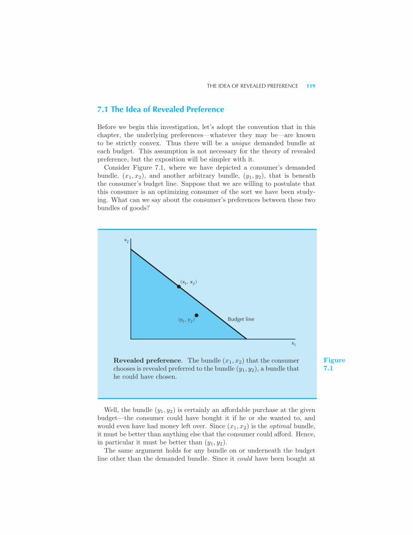
THE IDEA OF REVEALED PREFERENCE 119
7.1 The Idea of Revealed Preference
Before we begin this investigation, let’s adopt the convention that in thischapter, the underlying preferences—whatever they may be—are knownto be strictly convex. Thus there will be a unique demanded bundle ateach budget. This assumption is not necessary for the theory of revealedpreference, but the exposition will be simpler with it.Consider Figure 7.1, where we have depicted a consumer’s demanded
bundle, (x1, x2), and another arbitrary bundle, (y1, y2), that is beneaththe consumer’s budget line. Suppose that we are willing to postulate thatthis consumer is an optimizing consumer of the sort we have been study-ing. What can we say about the consumer’s preferences between these twobundles of goods?
x
(x , x )
(y , y ) Budget line
x
1 2
1 2
1
2
Revealed preference. The bundle (x1, x2) that the consumerchooses is revealed preferred to the bundle (y1, y2), a bundle thathe could have chosen.
Figure7.1
Well, the bundle (y1, y2) is certainly an affordable purchase at the givenbudget—the consumer could have bought it if he or she wanted to, andwould even have had money left over. Since (x1, x2) is the optimal bundle,it must be better than anything else that the consumer could afford. Hence,in particular it must be better than (y1, y2).The same argument holds for any bundle on or underneath the budget
line other than the demanded bundle. Since it could have been bought at
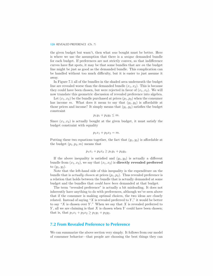
120 REVEALED PREFERENCE (Ch. 7)
the given budget but wasn’t, then what was bought must be better. Hereis where we use the assumption that there is a unique demanded bundlefor each budget. If preferences are not strictly convex, so that indifferencecurves have flat spots, it may be that some bundles that are on the budgetline might be just as good as the demanded bundle. This complication canbe handled without too much difficulty, but it is easier to just assume itaway.In Figure 7.1 all of the bundles in the shaded area underneath the budget
line are revealed worse than the demanded bundle (x1, x2). This is becausethey could have been chosen, but were rejected in favor of (x1, x2). We willnow translate this geometric discussion of revealed preference into algebra.Let (x1, x2) be the bundle purchased at prices (p1, p2) when the consumer
has income m. What does it mean to say that (y1, y2) is affordable atthose prices and income? It simply means that (y1, y2) satisfies the budgetconstraint
p1y1 + p2y2 ≤ m.
Since (x1, x2) is actually bought at the given budget, it must satisfy thebudget constraint with equality
p1x1 + p2x2 = m.
Putting these two equations together, the fact that (y1, y2) is affordable atthe budget (p1, p2,m) means that
p1x1 + p2x2 ≥ p1y1 + p2y2.
If the above inequality is satisfied and (y1, y2) is actually a differentbundle from (x1, x2), we say that (x1, x2) is directly revealed preferredto (y1, y2).Note that the left-hand side of this inequality is the expenditure on the
bundle that is actually chosen at prices (p1, p2). Thus revealed preference isa relation that holds between the bundle that is actually demanded at somebudget and the bundles that could have been demanded at that budget.The term “revealed preference” is actually a bit misleading. It does not
inherently have anything to do with preferences, although we’ve seen abovethat if the consumer is making optimal choices, the two ideas are closelyrelated. Instead of saying “X is revealed preferred to Y ,” it would be betterto say “X is chosen over Y .” When we say that X is revealed preferred toY , all we are claiming is that X is chosen when Y could have been chosen;that is, that p1x1 + p2x2 ≥ p1y1 + p2y2.
7.2 From Revealed Preference to Preference
We can summarize the above section very simply. It follows from our modelof consumer behavior—that people are choosing the best things they can
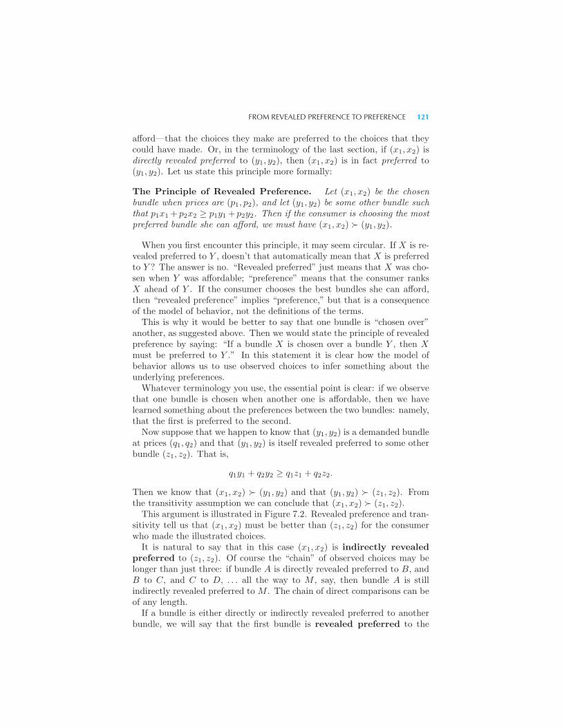
FROM REVEALED PREFERENCE TO PREFERENCE 121
afford—that the choices they make are preferred to the choices that theycould have made. Or, in the terminology of the last section, if (x1, x2) isdirectly revealed preferred to (y1, y2), then (x1, x2) is in fact preferred to(y1, y2). Let us state this principle more formally:
The Principle of Revealed Preference. Let (x1, x2) be the chosenbundle when prices are (p1, p2), and let (y1, y2) be some other bundle suchthat p1x1+ p2x2 ≥ p1y1+ p2y2. Then if the consumer is choosing the mostpreferred bundle she can afford, we must have (x1, x2) � (y1, y2).
When you first encounter this principle, it may seem circular. If X is re-vealed preferred to Y , doesn’t that automatically mean that X is preferredto Y ? The answer is no. “Revealed preferred” just means that X was cho-sen when Y was affordable; “preference” means that the consumer ranksX ahead of Y . If the consumer chooses the best bundles she can afford,then “revealed preference” implies “preference,” but that is a consequenceof the model of behavior, not the definitions of the terms.This is why it would be better to say that one bundle is “chosen over”
another, as suggested above. Then we would state the principle of revealedpreference by saying: “If a bundle X is chosen over a bundle Y , then Xmust be preferred to Y .” In this statement it is clear how the model ofbehavior allows us to use observed choices to infer something about theunderlying preferences.Whatever terminology you use, the essential point is clear: if we observe
that one bundle is chosen when another one is affordable, then we havelearned something about the preferences between the two bundles: namely,that the first is preferred to the second.Now suppose that we happen to know that (y1, y2) is a demanded bundle
at prices (q1, q2) and that (y1, y2) is itself revealed preferred to some otherbundle (z1, z2). That is,
q1y1 + q2y2 ≥ q1z1 + q2z2.
Then we know that (x1, x2) � (y1, y2) and that (y1, y2) � (z1, z2). Fromthe transitivity assumption we can conclude that (x1, x2) � (z1, z2).This argument is illustrated in Figure 7.2. Revealed preference and tran-
sitivity tell us that (x1, x2) must be better than (z1, z2) for the consumerwho made the illustrated choices.It is natural to say that in this case (x1, x2) is indirectly revealed
preferred to (z1, z2). Of course the “chain” of observed choices may belonger than just three: if bundle A is directly revealed preferred to B, andB to C, and C to D, . . . all the way to M , say, then bundle A is stillindirectly revealed preferred to M . The chain of direct comparisons can beof any length.If a bundle is either directly or indirectly revealed preferred to another
bundle, we will say that the first bundle is revealed preferred to the
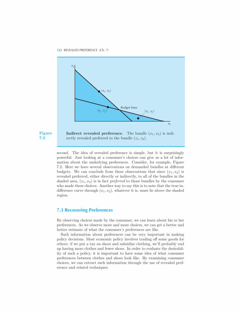
122 REVEALED PREFERENCE (Ch. 7)
(x , x
x2
1 2)
Budget lines21 21
1x
(y , y ) z , z( )
Figure7.2
Indirect revealed preference. The bundle (x1, x2) is indi-rectly revealed preferred to the bundle (z1, z2).
second. The idea of revealed preference is simple, but it is surprisinglypowerful. Just looking at a consumer’s choices can give us a lot of infor-mation about the underlying preferences. Consider, for example, Figure7.2. Here we have several observations on demanded bundles at differentbudgets. We can conclude from these observations that since (x1, x2) isrevealed preferred, either directly or indirectly, to all of the bundles in theshaded area, (x1, x2) is in fact preferred to those bundles by the consumerwho made these choices. Another way to say this is to note that the true in-difference curve through (x1, x2), whatever it is, must lie above the shadedregion.
7.3 Recovering Preferences
By observing choices made by the consumer, we can learn about his or herpreferences. As we observe more and more choices, we can get a better andbetter estimate of what the consumer’s preferences are like.Such information about preferences can be very important in making
policy decisions. Most economic policy involves trading off some goods forothers: if we put a tax on shoes and subsidize clothing, we’ll probably endup having more clothes and fewer shoes. In order to evaluate the desirabil-ity of such a policy, it is important to have some idea of what consumerpreferences between clothes and shoes look like. By examining consumerchoices, we can extract such information through the use of revealed pref-erence and related techniques.
RECOVERING PREFERENCES 123
If we are willing to add more assumptions about consumer preferences,we can get more precise estimates about the shape of indifference curves.For example, suppose we observe two bundles Y and Z that are revealedpreferred to X, as in Figure 7.3, and that we are willing to postulatepreferences are convex. Then we know that all of the weighted averagesof Y and Z are preferred to X as well. If we are willing to assume thatpreferences are monotonic, then all the bundles that have more of bothgoods than X, Y , and Z—or any of their weighted averages—are alsopreferred to X.
Betterbundles
Possibleindifferencecurve
Budgetlines
Worsebundles
Y
X
Z
x
x2
1
Trapping the indifference curve. The upper shaded areaconsists of bundles preferred to X, and the lower shaded areaconsists of bundles revealed worse than X. The indifferencecurve through X must lie somewhere in the region between thetwo shaded areas.
Figure7.3
The region labeled “Worse bundles” in Figure 7.3 consists of all thebundles to which X is revealed preferred. That is, this region consists ofall the bundles that cost less than X, along with all the bundles that costless than bundles that cost less than X, and so on.
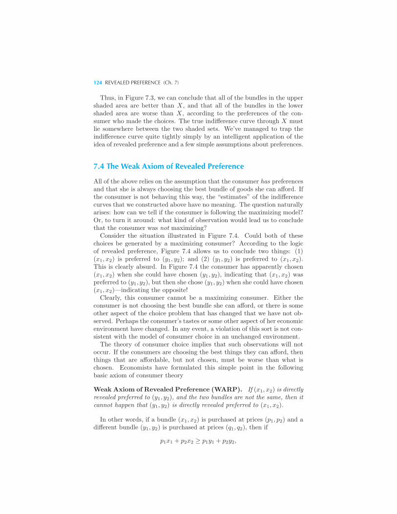
124 REVEALED PREFERENCE (Ch. 7)
Thus, in Figure 7.3, we can conclude that all of the bundles in the uppershaded area are better than X, and that all of the bundles in the lowershaded area are worse than X, according to the preferences of the con-sumer who made the choices. The true indifference curve through X mustlie somewhere between the two shaded sets. We’ve managed to trap theindifference curve quite tightly simply by an intelligent application of theidea of revealed preference and a few simple assumptions about preferences.
7.4 The Weak Axiom of Revealed Preference
All of the above relies on the assumption that the consumer has preferencesand that she is always choosing the best bundle of goods she can afford. Ifthe consumer is not behaving this way, the “estimates” of the indifferencecurves that we constructed above have no meaning. The question naturallyarises: how can we tell if the consumer is following the maximizing model?Or, to turn it around: what kind of observation would lead us to concludethat the consumer was not maximizing?
Consider the situation illustrated in Figure 7.4. Could both of thesechoices be generated by a maximizing consumer? According to the logicof revealed preference, Figure 7.4 allows us to conclude two things: (1)(x1, x2) is preferred to (y1, y2); and (2) (y1, y2) is preferred to (x1, x2).This is clearly absurd. In Figure 7.4 the consumer has apparently chosen(x1, x2) when she could have chosen (y1, y2), indicating that (x1, x2) waspreferred to (y1, y2), but then she chose (y1, y2) when she could have chosen(x1, x2)—indicating the opposite!Clearly, this consumer cannot be a maximizing consumer. Either the
consumer is not choosing the best bundle she can afford, or there is someother aspect of the choice problem that has changed that we have not ob-served. Perhaps the consumer’s tastes or some other aspect of her economicenvironment have changed. In any event, a violation of this sort is not con-sistent with the model of consumer choice in an unchanged environment.The theory of consumer choice implies that such observations will not
occur. If the consumers are choosing the best things they can afford, thenthings that are affordable, but not chosen, must be worse than what ischosen. Economists have formulated this simple point in the followingbasic axiom of consumer theory
Weak Axiom of Revealed Preference (WARP). If (x1, x2) is directlyrevealed preferred to (y1, y2), and the two bundles are not the same, then itcannot happen that (y1, y2) is directly revealed preferred to (x1, x2).
In other words, if a bundle (x1, x2) is purchased at prices (p1, p2) and adifferent bundle (y1, y2) is purchased at prices (q1, q2), then if
p1x1 + p2x2 ≥ p1y1 + p2y2,
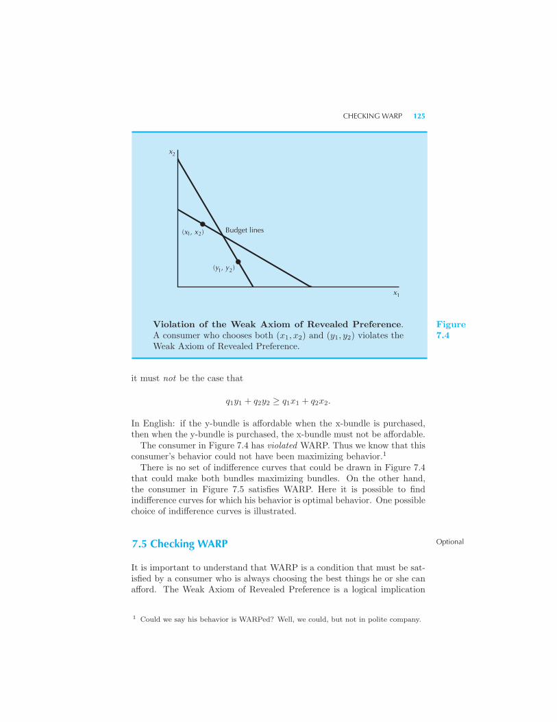
CHECKING WARP 125
1x
Budget lines
21(y , y )
21(x , x )
x2
Violation of the Weak Axiom of Revealed Preference.A consumer who chooses both (x1, x2) and (y1, y2) violates theWeak Axiom of Revealed Preference.
Figure7.4
it must not be the case that
q1y1 + q2y2 ≥ q1x1 + q2x2.
In English: if the y-bundle is affordable when the x-bundle is purchased,then when the y-bundle is purchased, the x-bundle must not be affordable.The consumer in Figure 7.4 has violated WARP. Thus we know that this
consumer’s behavior could not have been maximizing behavior.1
There is no set of indifference curves that could be drawn in Figure 7.4that could make both bundles maximizing bundles. On the other hand,the consumer in Figure 7.5 satisfies WARP. Here it is possible to findindifference curves for which his behavior is optimal behavior. One possiblechoice of indifference curves is illustrated.
Optional7.5 Checking WARP
It is important to understand that WARP is a condition that must be sat-isfied by a consumer who is always choosing the best things he or she canafford. The Weak Axiom of Revealed Preference is a logical implication
1 Could we say his behavior is WARPed? Well, we could, but not in polite company.
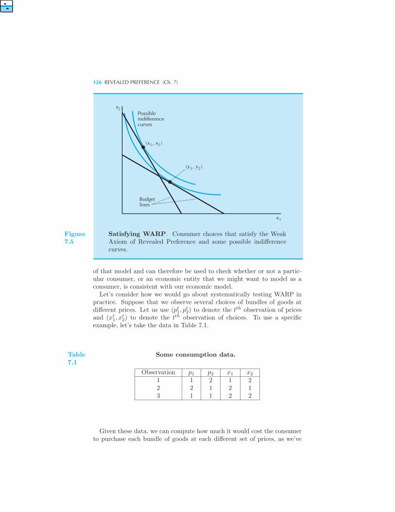
126 REVEALED PREFERENCE (Ch. 7)
Possibleindifferencecurves
x2
Budgetlines
1x
(x , x )1 2
1 2(y , y )
Figure7.5
Satisfying WARP. Consumer choices that satisfy the WeakAxiom of Revealed Preference and some possible indifferencecurves.
of that model and can therefore be used to check whether or not a partic-ular consumer, or an economic entity that we might want to model as aconsumer, is consistent with our economic model.Let’s consider how we would go about systematically testing WARP in
practice. Suppose that we observe several choices of bundles of goods atdifferent prices. Let us use (pt1, p
t2) to denote the tth observation of prices
and (xt1, x
t2) to denote the tth observation of choices. To use a specific
example, let’s take the data in Table 7.1.
Table7.1
Some consumption data.
Observation p1 p2 x1 x2
1 1 2 1 22 2 1 2 13 1 1 2 2
Given these data, we can compute how much it would cost the consumerto purchase each bundle of goods at each different set of prices, as we’ve
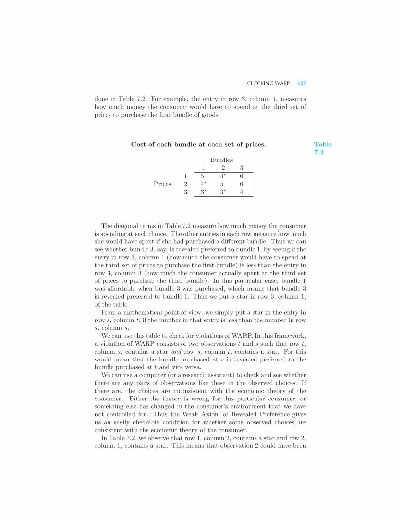
CHECKING WARP 127
done in Table 7.2. For example, the entry in row 3, column 1, measureshow much money the consumer would have to spend at the third set ofprices to purchase the first bundle of goods.
Cost of each bundle at each set of prices.
Bundles1 2 3
1 5 4∗ 6Prices 2 4∗ 5 6
3 3∗ 3∗ 4
Table7.2
The diagonal terms in Table 7.2 measure how much money the consumeris spending at each choice. The other entries in each row measure how muchshe would have spent if she had purchased a different bundle. Thus we cansee whether bundle 3, say, is revealed preferred to bundle 1, by seeing if theentry in row 3, column 1 (how much the consumer would have to spend atthe third set of prices to purchase the first bundle) is less than the entry inrow 3, column 3 (how much the consumer actually spent at the third setof prices to purchase the third bundle). In this particular case, bundle 1was affordable when bundle 3 was purchased, which means that bundle 3is revealed preferred to bundle 1. Thus we put a star in row 3, column 1,of the table.From a mathematical point of view, we simply put a star in the entry in
row s, column t, if the number in that entry is less than the number in rows, column s.
We can use this table to check for violations of WARP. In this framework,a violation of WARP consists of two observations t and s such that row t,column s, contains a star and row s, column t, contains a star. For thiswould mean that the bundle purchased at s is revealed preferred to thebundle purchased at t and vice versa.We can use a computer (or a research assistant) to check and see whether
there are any pairs of observations like these in the observed choices. Ifthere are, the choices are inconsistent with the economic theory of theconsumer. Either the theory is wrong for this particular consumer, orsomething else has changed in the consumer’s environment that we havenot controlled for. Thus the Weak Axiom of Revealed Preference givesus an easily checkable condition for whether some observed choices areconsistent with the economic theory of the consumer.In Table 7.2, we observe that row 1, column 2, contains a star and row 2,
column 1, contains a star. This means that observation 2 could have been
128 REVEALED PREFERENCE (Ch. 7)
chosen when the consumer actually chose observation 1 and vice versa. Thisis a violation of the Weak Axiom of Revealed Preference. We can concludethat the data depicted in Tables 7.1 and 7.2 could not be generated by aconsumer with stable preferences who was always choosing the best thingshe or she could afford.
7.6 The Strong Axiom of Revealed Preference
The Weak Axiom of Revealed Preference described in the last section givesus an observable condition that must be satisfied by all optimizing con-sumers. But there is a stronger condition that is sometimes useful.We have already noted that if a bundle of goods X is revealed preferred
to a bundle Y , and Y is in turn revealed preferred to a bundle Z, then Xmust in fact be preferred to Z. If the consumer has consistent preferences,then we should never observe a sequence of choices that would reveal thatZ was preferred to X.The Weak Axiom of Revealed Preference requires that if X is directly
revealed preferred to Y , then we should never observe Y being directlyrevealed preferred to X. The Strong Axiom of Revealed Preference(SARP) requires that the same sort of condition hold for indirect revealedpreference. More formally, we have the following.
Strong Axiom of Revealed Preference (SARP). If (x1, x2) is re-vealed preferred to (y1, y2) (either directly or indirectly) and (y1, y2) is dif-ferent from (x1, x2), then (y1, y2) cannot be directly or indirectly revealedpreferred to (x1, x2).
It is clear that if the observed behavior is optimizing behavior then itmust satisfy the SARP. For if the consumer is optimizing and (x1, x2)is revealed preferred to (y1, y2), either directly or indirectly, then we musthave (x1, x2) � (y1, y2). So having (x1, x2) revealed preferred to (y1, y2) and(y1, y2) revealed preferred to (x1, x2) would imply that (x1, x2) � (y1, y2)and (y1, y2) � (x1, x2), which is a contradiction. We can conclude thateither the consumer must not be optimizing, or some other aspect of theconsumer’s environment—such as tastes, other prices, and so on—musthave changed.Roughly speaking, since the underlying preferences of the consumer must
be transitive, it follows that the revealed preferences of the consumer mustbe transitive. Thus SARP is a necessary implication of optimizing behav-ior: if a consumer is always choosing the best things that he can afford,then his observed behavior must satisfy SARP. What is more surprising isthat any behavior satisfying the Strong Axiom can be thought of as beinggenerated by optimizing behavior in the following sense: if the observedchoices satisfy SARP, we can always find nice, well-behaved preferences
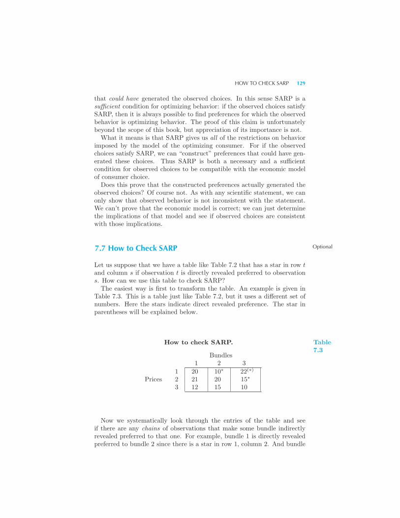
HOW TO CHECK SARP 129
that could have generated the observed choices. In this sense SARP is asufficient condition for optimizing behavior: if the observed choices satisfySARP, then it is always possible to find preferences for which the observedbehavior is optimizing behavior. The proof of this claim is unfortunatelybeyond the scope of this book, but appreciation of its importance is not.What it means is that SARP gives us all of the restrictions on behavior
imposed by the model of the optimizing consumer. For if the observedchoices satisfy SARP, we can “construct” preferences that could have gen-erated these choices. Thus SARP is both a necessary and a sufficientcondition for observed choices to be compatible with the economic modelof consumer choice.Does this prove that the constructed preferences actually generated the
observed choices? Of course not. As with any scientific statement, we canonly show that observed behavior is not inconsistent with the statement.We can’t prove that the economic model is correct; we can just determinethe implications of that model and see if observed choices are consistentwith those implications.
Optional7.7 How to Check SARP
Let us suppose that we have a table like Table 7.2 that has a star in row tand column s if observation t is directly revealed preferred to observations. How can we use this table to check SARP?
The easiest way is first to transform the table. An example is given inTable 7.3. This is a table just like Table 7.2, but it uses a different set ofnumbers. Here the stars indicate direct revealed preference. The star inparentheses will be explained below.
How to check SARP.
Bundles1 2 3
1 20 10∗ 22(∗)
Prices 2 21 20 15∗
3 12 15 10
Table7.3
Now we systematically look through the entries of the table and seeif there are any chains of observations that make some bundle indirectlyrevealed preferred to that one. For example, bundle 1 is directly revealedpreferred to bundle 2 since there is a star in row 1, column 2. And bundle
130 REVEALED PREFERENCE (Ch. 7)
2 is directly revealed preferred to bundle 3, since there is a star in row 2,column 3. Therefore bundle 1 is indirectly revealed preferred to bundle 3,and we indicate this by putting a star (in parentheses) in row 1, column 3.
In general, if we have many observations, we will have to look for chainsof arbitrary length to see if one observation is indirectly revealed preferredto another. Although it may not be exactly obvious how to do this, itturns out that there are simple computer programs that can calculate theindirect revealed preference relation from the table describing the directrevealed preference relation. The computer can put a star in location stof the table if observation s is revealed preferred to observation t by anychain of other observations.
Once we have done this calculation, we can easily test for SARP. We justsee if there is a situation where there is a star in row t, column s, and also astar in row s, column t. If so, we have found a situation where observationt is revealed preferred to observation s, either directly or indirectly, and,at the same time, observation s is revealed preferred to observation t. Thisis a violation of the Strong Axiom of Revealed Preference.
On the other hand, if we do not find such violations, then we know thatthe observations we have are consistent with the economic theory of theconsumer. These observations could have been made by an optimizingconsumer with well-behaved preferences. Thus we have a completely op-erational test for whether or not a particular consumer is acting in a wayconsistent with economic theory.
This is important, since we can model several kinds of economic units asbehaving like consumers. Think, for example, of a household consisting ofseveral people. Will its consumption choices maximize “household utility”?If we have some data on household consumption choices, we can use theStrong Axiom of Revealed Preference to see. Another economic unit thatwe might think of as acting like a consumer is a nonprofit organizationlike a hospital or a university. Do universities maximize a utility func-tion in making their economic choices? If we have a list of the economicchoices that a university makes when faced with different prices, we can,in principle, answer this kind of question.
7.8 Index Numbers
Suppose we examine the consumption bundles of a consumer at two differ-ent times and we want to compare how consumption has changed from onetime to the other. Let b stand for the base period, and let t be some othertime. How does “average” consumption in year t compare to consumptionin the base period?
Suppose that at time t prices are (pt1, pt2) and that the consumer chooses
(xt1, x
t2). In the base period b, the prices are (pb1, p
b2), and the consumer’s
INDEX NUMBERS 131
choice is (xb1, x
b2). We want to ask how the “average” consumption of the
consumer has changed.If we let w1 and w2 be some “weights” that go into making an average,
then we can look at the following kind of quantity index:
Iq =w1x
t1 + w2x
t2
w1xb1 + w2xb
2
.
If Iq is greater than 1, we can say that the “average” consumption has goneup in the movement from b to t; if Iq is less than 1, we can say that the“average” consumption has gone down.The question is, what do we use for the weights? A natural choice is to
use the prices of the goods in question, since they measure in some sensethe relative importance of the two goods. But there are two sets of priceshere: which should we use?If we use the base period prices for the weights, we have something called
a Laspeyres index, and if we use the t period prices, we have somethingcalled a Paasche index. Both of these indices answer the question of whathas happened to “average” consumption, but they just use different weightsin the averaging process.Substituting the t period prices for the weights, we see that the Paasche
quantity index is given by
Pq =pt1x
t1 + pt2x
t2
pt1xb1 + pt2x
b2
,
and substituting the b period prices shows that the Laspeyres quantityindex is given by
Lq =pb1x
t1 + pb2x
t2
pb1xb1 + pb2x
b2
.
It turns out that the magnitude of the Laspeyres and Paasche indices cantell us something quite interesting about the consumer’s welfare. Supposethat we have a situation where the Paasche quantity index is greater than 1:
Pq =pt1x
t1 + pt2x
t2
pt1xb1 + pt2x
b2
> 1.
What can we conclude about how well-off the consumer is at time t ascompared to his situation at time b?
The answer is provided by revealed preference. Just cross multiply thisinequality to give
pt1xt1 + pt2x
t2 > pt1x
b1 + pt2x
b2,
which immediately shows that the consumer must be better off at t than atb, since he could have consumed the b consumption bundle in the t situationbut chose not to do so.
132 REVEALED PREFERENCE (Ch. 7)
What if the Paasche index is less than 1? Then we would have
pt1xt1 + pt2x
t2 < pt1x
b1 + pt2x
b2,
which says that when the consumer chose bundle (xt1, x
t2), bundle (xb
1, xb2)
was not affordable. But that doesn’t say anything about the consumer’sranking of the bundles. Just because something costs more than you canafford doesn’t mean that you prefer it to what you’re consuming now.What about the Laspeyres index? It works in a similar way. Suppose
that the Laspeyres index is less than 1:
Lq =pb1x
t1 + pb2x
t2
pb1xb1 + pb2x
b2
< 1.
Cross multiplying yields
pb1xb1 + pb2x
b2 > pb1x
t1 + pb2x
t2,
which says that (xb1, x
b2) is revealed preferred to (xt
1, xt2). Thus the consumer
is better off at time b than at time t.
7.9 Price Indices
Price indices work in much the same way. In general, a price index will bea weighted average of prices:
Ip =pt1w1 + pt2w2
pb1w1 + pb2w2.
In this case it is natural to choose the quantities as the weights for com-puting the averages. We get two different indices, depending on our choiceof weights. If we choose the t period quantities for weights, we get thePaasche price index:
Pp =pt1x
t1 + pt2x
t2
pb1xt1 + pb2x
t2
,
and if we choose the base period quantities we get the Laspeyres priceindex:
Lp =pt1x
b1 + pt2x
b2
pb1xb1 + pb2x
b2
.
Suppose that the Paasche price index is less than 1; what does revealedpreference have to say about the welfare situation of the consumer in peri-ods t and b?
PRICE INDICES 133
Revealed preference doesn’t say anything at all. The problem is thatthere are now different prices in the numerator and in the denominator ofthe fractions defining the indices, so the revealed preference comparisoncan’t be made.Let’s define a new index of the change in total expenditure by
M =pt1x
t1 + pt2x
t2
pb1xb1 + pb2x
b2
.
This is the ratio of total expenditure in period t to the total expenditurein period b.Now suppose that you are told that the Paasche price index was greater
than M . This means that
Pp =pt1x
t1 + pt2x
t2
pb1xt1 + pb2x
t2
>pt1x
t1 + pt2x
t2
pb1xb1 + pb2x
b2
.
Canceling the numerators from each side of this expression and cross mul-tiplying, we have
pb1xb1 + pb2x
b2 > pb1x
t1 + pb2x
t2.
This statement says that the bundle chosen at year b is revealed preferredto the bundle chosen at year t. This analysis implies that if the Paascheprice index is greater than the expenditure index, then the consumer mustbe better off in year b than in year t.
This is quite intuitive. After all, if prices rise by more than income risesin the movement from b to t, we would expect that would tend to make theconsumer worse off. The revealed preference analysis given above confirmsthis intuition.A similar statement can be made for the Laspeyres price index. If the
Laspeyres price index is less than M , then the consumer must be better offin year t than in year b. Again, this simply confirms the intuitive idea thatif prices rise less than income, the consumer would become better off. Inthe case of price indices, what matters is not whether the index is greateror less than 1, but whether it is greater or less than the expenditure index.
EXAMPLE: Indexing Social Security Payments
Many elderly people have Social Security payments as their sole sourceof income. Because of this, there have been attempts to adjust SocialSecurity payments in a way that will keep purchasing power constant evenwhen prices change. Since the amount of payments will then depend on themovement of some price index or cost-of-living index, this kind of schemeis referred to as indexing.
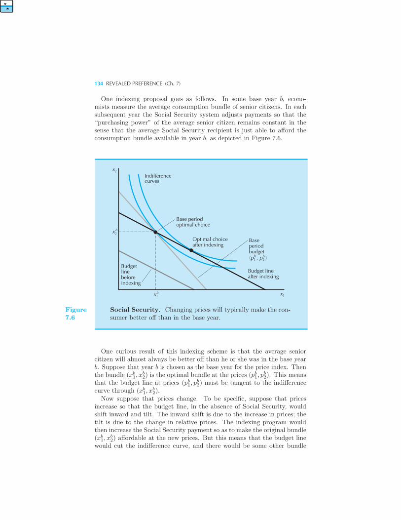
134 REVEALED PREFERENCE (Ch. 7)
One indexing proposal goes as follows. In some base year b, econo-mists measure the average consumption bundle of senior citizens. In eachsubsequent year the Social Security system adjusts payments so that the“purchasing power” of the average senior citizen remains constant in thesense that the average Social Security recipient is just able to afford theconsumption bundle available in year b, as depicted in Figure 7.6.
x2
x2b
1xb1x
Budgetline beforeindexing
Indifferencecurves
Base periodoptimal choice
Optimal choiceafter indexing
Budget lineafter indexing
Baseperiodbudget(p , p )1 2
b b
Figure7.6
Social Security. Changing prices will typically make the con-sumer better off than in the base year.
One curious result of this indexing scheme is that the average seniorcitizen will almost always be better off than he or she was in the base yearb. Suppose that year b is chosen as the base year for the price index. Thenthe bundle (xb
1, xb2) is the optimal bundle at the prices (pb1, p
b2). This means
that the budget line at prices (pb1, pb2) must be tangent to the indifference
curve through (xb1, x
b2).
Now suppose that prices change. To be specific, suppose that pricesincrease so that the budget line, in the absence of Social Security, wouldshift inward and tilt. The inward shift is due to the increase in prices; thetilt is due to the change in relative prices. The indexing program wouldthen increase the Social Security payment so as to make the original bundle(xb
1, xb2) affordable at the new prices. But this means that the budget line
would cut the indifference curve, and there would be some other bundle
REVIEW QUESTIONS 135
on the budget line that would be strictly preferred to (xb1, x
b2). Thus the
consumer would typically be able to choose a better bundle than he or shechose in the base year.
Summary
1. If one bundle is chosen when another could have been chosen, we saythat the first bundle is revealed preferred to the second.
2. If the consumer is always choosing the most preferred bundles he or shecan afford, this means that the chosen bundles must be preferred to thebundles that were affordable but weren’t chosen.
3. Observing the choices of consumers can allow us to “recover” or esti-mate the preferences that lie behind those choices. The more choices weobserve, the more precisely we can estimate the underlying preferences thatgenerated those choices.
4. The Weak Axiom of Revealed Preference (WARP) and the Strong Ax-iom of Revealed Preference (SARP) are necessary conditions that consumerchoices have to obey if they are to be consistent with the economic modelof optimizing choice.
REVIEW QUESTIONS
1. When prices are (p1, p2) = (1, 2) a consumer demands (x1, x2) = (1, 2),and when prices are (q1, q2) = (2, 1) the consumer demands (y1, y2) = (2, 1).Is this behavior consistent with the model of maximizing behavior?
2. When prices are (p1, p2) = (2, 1) a consumer demands (x1, x2) = (1, 2),and when prices are (q1, q2) = (1, 2) the consumer demands (y1, y2) = (2, 1).Is this behavior consistent with the model of maximizing behavior?
3. In the preceding exercise, which bundle is preferred by the consumer,the x-bundle or the y-bundle?
4. We saw that the Social Security adjustment for changing prices wouldtypically make recipients at least as well-off as they were at the base year.What kind of price changes would leave them just as well-off, no matterwhat kind of preferences they had?
5. In the same framework as the above question, what kind of preferenceswould leave the consumer just as well-off as he was in the base year, for allprice changes?
CHAPTER 8
SLUTSKYEQUATION
Economists often are concerned with how a consumer’s behavior changesin response to changes in the economic environment. The case we wantto consider in this chapter is how a consumer’s choice of a good respondsto changes in its price. It is natural to think that when the price of agood rises the demand for it will fall. However, as we saw in Chapter 6it is possible to construct examples where the optimal demand for a gooddecreases when its price falls. A good that has this property is called aGiffen good.Giffen goods are pretty peculiar and are primarily a theoretical curiosity,
but there are other situations where changes in prices might have “perverse”effects that, on reflection, turn out not to be so unreasonable. For example,we normally think that if people get a higher wage they will work more.But what if your wage went from $10 an hour to $1000 an hour? Wouldyou really work more? Might you not decide to work fewer hours and usesome of the money you’ve earned to do other things? What if your wagewere $1,000,000 an hour? Wouldn’t you work less?For another example, think of what happens to your demand for apples
when the price goes up. You would probably consume fewer apples. But
THE SUBSTITUTION EFFECT 137
how about a family who grew apples to sell? If the price of apples wentup, their income might go up so much that they would feel that they couldnow afford to consume more of their own apples. For the consumers in thisfamily, an increase in the price of apples might well lead to an increase inthe consumption of apples.What is going on here? How is it that changes in price can have these
ambiguous effects on demand? In this chapter and the next we’ll try tosort out these effects.
8.1 The Substitution Effect
When the price of a good changes, there are two sorts of effects: the rateat which you can exchange one good for another changes, and the totalpurchasing power of your income is altered. If, for example, good 1 becomescheaper, it means that you have to give up less of good 2 to purchase good1. The change in the price of good 1 has changed the rate at which themarket allows you to “substitute” good 2 for good 1. The trade-off betweenthe two goods that the market presents the consumer has changed.At the same time, if good 1 becomes cheaper it means that your money
income will buy more of good 1. The purchasing power of your money hasgone up; although the number of dollars you have is the same, the amountthat they will buy has increased.The first part—the change in demand due to the change in the rate
of exchange between the two goods—is called the substitution effect.The second effect—the change in demand due to having more purchasingpower—is called the income effect. These are only rough definitions of thetwo effects. In order to give a more precise definition we have to considerthe two effects in greater detail.The way that we will do this is to break the price movement into two
steps: first we will let the relative prices change and adjust money incomeso as to hold purchasing power constant, then we will let purchasing poweradjust while holding the relative prices constant.This is best explained by referring to Figure 8.1. Here we have a situa-
tion where the price of good 1 has declined. This means that the budgetline rotates around the vertical intercept m/p2 and becomes flatter. Wecan break this movement of the budget line up into two steps: first pivotthe budget line around the original demanded bundle and then shift thepivoted line out to the new demanded bundle.
This “pivot-shift” operation gives us a convenient way to decomposethe change in demand into two pieces. The first step—the pivot—is amovement where the slope of the budget line changes while its purchasingpower stays constant, while the second step is a movement where the slopestays constant and the purchasing power changes. This decomposition isonly a hypothetical construction—the consumer simply observes a change
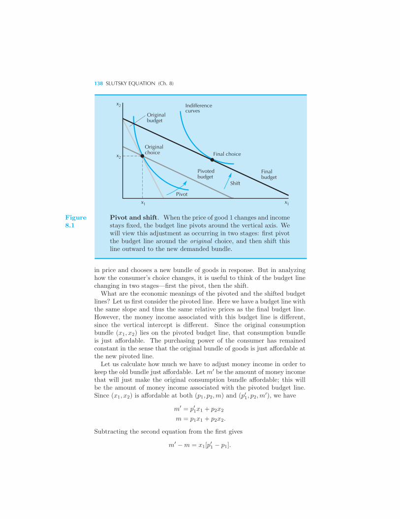
138 SLUTSKY EQUATION (Ch. 8)
x
x
Shift
Pivot
2
1x1
x2
Originalbudget
Indifferencecurves
Final choice
Final budget
Pivotedbudget
Originalchoice
Figure8.1
Pivot and shift. When the price of good 1 changes and incomestays fixed, the budget line pivots around the vertical axis. Wewill view this adjustment as occurring in two stages: first pivotthe budget line around the original choice, and then shift thisline outward to the new demanded bundle.
in price and chooses a new bundle of goods in response. But in analyzinghow the consumer’s choice changes, it is useful to think of the budget linechanging in two stages—first the pivot, then the shift.What are the economic meanings of the pivoted and the shifted budget
lines? Let us first consider the pivoted line. Here we have a budget line withthe same slope and thus the same relative prices as the final budget line.However, the money income associated with this budget line is different,since the vertical intercept is different. Since the original consumptionbundle (x1, x2) lies on the pivoted budget line, that consumption bundleis just affordable. The purchasing power of the consumer has remainedconstant in the sense that the original bundle of goods is just affordable atthe new pivoted line.Let us calculate how much we have to adjust money income in order to
keep the old bundle just affordable. Let m′ be the amount of money incomethat will just make the original consumption bundle affordable; this willbe the amount of money income associated with the pivoted budget line.Since (x1, x2) is affordable at both (p1, p2,m) and (p′1, p2,m
′), we have
m′ = p′1x1 + p2x2
m = p1x1 + p2x2.
Subtracting the second equation from the first gives
m′ −m = x1[p′1 − p1].
THE SUBSTITUTION EFFECT 139
This equation says that the change in money income necessary to makethe old bundle affordable at the new prices is just the original amount ofconsumption of good 1 times the change in prices.Letting Δp1 = p′1 − p1 represent the change in price 1, and Δm =
m′ −m represent the change in income necessary to make the old bundlejust affordable, we have
Δm = x1Δp1. (8.1)
Note that the change in income and the change in price will always movein the same direction: if the price goes up, then we have to raise income tokeep the same bundle affordable.Let’s use some actual numbers. Suppose that the consumer is originally
consuming 20 candy bars a week, and that candy bars cost 50 cents a piece.If the price of candy bars goes up by 10 cents—so that Δp1 = .60− .50 =.10—how much would income have to change to make the old consumptionbundle affordable?We can apply the formula given above. If the consumer had $2.00 more
income, he would just be able to consume the same number of candy bars,namely, 20. In terms of the formula:
Δm = Δp1 × x1 = .10× 20 = $2.00.
Now we have a formula for the pivoted budget line: it is just the budgetline at the new price with income changed by Δm. Note that if the price ofgood 1 goes down, then the adjustment in income will be negative. Whena price goes down, a consumer’s purchasing power goes up, so we will haveto decrease the consumer’s income in order to keep purchasing power fixed.Similarly, when a price goes up, purchasing power goes down, so the changein income necessary to keep purchasing power constant must be positive.Although (x1, x2) is still affordable, it is not generally the optimal pur-
chase at the pivoted budget line. In Figure 8.2 we have denoted the optimalpurchase on the pivoted budget line by Y . This bundle of goods is the op-timal bundle of goods when we change the price and then adjust dollarincome so as to keep the old bundle of goods just affordable. The move-ment from X to Y is known as the substitution effect. It indicates howthe consumer “substitutes” one good for the other when a price changesbut purchasing power remains constant.More precisely, the substitution effect, Δxs
1, is the change in the demandfor good 1 when the price of good 1 changes to p′1 and, at the same time,money income changes to m′:
Δxs1 = x1(p
′1,m
′)− x1(p1,m).
In order to determine the substitution effect, we must use the consumer’sdemand function to calculate the optimal choices at (p′1,m
′) and (p1,m).The change in the demand for good 1 may be large or small, depending
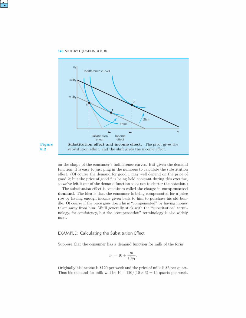
140 SLUTSKY EQUATION (Ch. 8)
x
m/p
m'/p
X
Y
Z
x
Substitutioneffect
Incomeeffect
ShiftPivot
Indifference curves2
2
2
1
Figure8.2
Substitution effect and income effect. The pivot gives thesubstitution effect, and the shift gives the income effect.
on the shape of the consumer’s indifference curves. But given the demandfunction, it is easy to just plug in the numbers to calculate the substitutioneffect. (Of course the demand for good 1 may well depend on the price ofgood 2; but the price of good 2 is being held constant during this exercise,so we’ve left it out of the demand function so as not to clutter the notation.)
The substitution effect is sometimes called the change in compensateddemand. The idea is that the consumer is being compensated for a pricerise by having enough income given back to him to purchase his old bun-dle. Of course if the price goes down he is “compensated” by having moneytaken away from him. We’ll generally stick with the “substitution” termi-nology, for consistency, but the “compensation” terminology is also widelyused.
EXAMPLE: Calculating the Substitution Effect
Suppose that the consumer has a demand function for milk of the form
x1 = 10 +m
10p1.
Originally his income is $120 per week and the price of milk is $3 per quart.Thus his demand for milk will be 10 + 120/(10× 3) = 14 quarts per week.
THE INCOME EFFECT 141
Now suppose that the price of milk falls to $2 per quart. Then hisdemand at this new price will be 10+120/(10× 2) = 16 quarts of milk perweek. The total change in demand is +2 quarts a week.In order to calculate the substitution effect, we must first calculate how
much income would have to change in order to make the original consump-tion of milk just affordable when the price of milk is $2 a quart. We applythe formula (8.1):
Δm = x1Δp1 = 14× (2− 3) = −$14.
Thus the level of income necessary to keep purchasing power constantis m′ = m + Δm = 120 − 14 = 106. What is the consumer’s demand formilk at the new price, $2 per quart, and this level of income? Just plugthe numbers into the demand function to find
x1(p′1,m
′) = x1(2, 106) = 10 +106
10× 2= 15.3.
Thus the substitution effect is
Δxs1 = x1(2, 106)− x1(3, 120) = 15.3− 14 = 1.3.
8.2 The Income Effect
We turn now to the second stage of the price adjustment—the shift move-ment. This is also easy to interpret economically. We know that a parallelshift of the budget line is the movement that occurs when income changeswhile relative prices remain constant. Thus the second stage of the priceadjustment is called the income effect. We simply change the consumer’sincome from m′ to m, keeping the prices constant at (p′1, p2). In Figure8.2 this change moves us from the point (y1, y2) to (z1, z2). It is natural tocall this last movement the income effect since all we are doing is changingincome while keeping the prices fixed at the new prices.More precisely, the income effect, Δxn
1 , is the change in the demand forgood 1 when we change income from m′ to m, holding the price of good 1fixed at p′1:
Δxn1 = x1(p
′1,m)− x1(p
′1,m
′).
We have already considered the income effect earlier in section 6.1. Therewe saw that the income effect can operate either way: it will tend to increaseor decrease the demand for good 1 depending on whether we have a normalgood or an inferior good.When the price of a good decreases, we need to decrease income in order
to keep purchasing power constant. If the good is a normal good, thenthis decrease in income will lead to a decrease in demand. If the good isan inferior good, then the decrease in income will lead to an increase indemand.
142 SLUTSKY EQUATION (Ch. 8)
EXAMPLE: Calculating the Income Effect
In the example given earlier in this chapter we saw that
x1(p′1,m) = x1(2, 120) = 16
x1(p′1,m
′) = x1(2, 106) = 15.3.
Thus the income effect for this problem is
Δxn1 = x1(2, 120)− x1(2, 106) = 16− 15.3 = 0.7.
Since milk is a normal good for this consumer, the demand for milk in-creases when income increases.
8.3 Sign of the Substitution Effect
We have seen above that the income effect can be positive or negative, de-pending on whether the good is a normal good or an inferior good. Whatabout the substitution effect? If the price of a good goes down, as inFigure 8.2, then the change in the demand for the good due to the substi-tution effect must be nonnegative. That is, if p1 > p′1, then we must havex1(p
′1,m
′) ≥ x1(p1,m), so that Δxs1 ≥ 0.
The proof of this goes as follows. Consider the points on the pivotedbudget line in Figure 8.2 where the amount of good 1 consumed is lessthan at the bundle X. These bundles were all affordable at the old prices(p1, p2) but they weren’t purchased. Instead the bundle X was purchased.If the consumer is always choosing the best bundle he can afford, then Xmust be preferred to all of the bundles on the part of the pivoted line thatlies inside the original budget set.
This means that the optimal choice on the pivoted budget line must notbe one of the bundles that lies underneath the original budget line. Theoptimal choice on the pivoted line would have to be either X or some pointto the right of X. But this means that the new optimal choice must involveconsuming at least as much of good 1 as originally, just as we wanted toshow. In the case illustrated in Figure 8.2, the optimal choice at the pivotedbudget line is the bundle Y , which certainly involves consuming more ofgood 1 than at the original consumption point, X.
The substitution effect always moves opposite to the price movement.We say that the substitution effect is negative, since the change in demanddue to the substitution effect is opposite to the change in price: if the priceincreases, the demand for the good due to the substitution effect decreases.
THE TOTAL CHANGE IN DEMAND 143
8.4 The Total Change in Demand
The total change in demand, Δx1, is the change in demand due to thechange in price, holding income constant:
Δx1 = x1(p′1,m)− x1(p1,m).
We have seen above how this change can be broken up into two changes: thesubstitution effect and the income effect. In terms of the symbols definedabove,
Δx1 = Δxs1 +Δxn
1
x1(p′1,m)− x1(p1,m) = [x1(p
′1,m
′)− x1(p1,m)]
+ [x1(p′1,m)− x1(p
′1,m
′)].
In words this equation says that the total change in demand equals thesubstitution effect plus the income effect. This equation is called the Slut-sky identity.1 Note that it is an identity: it is true for all values of p1,p′1, m, and m′. The first and fourth terms on the right-hand side cancelout, so the right-hand side is identically equal to the left-hand side.The content of the Slutsky identity is not just the algebraic identity—
that is a mathematical triviality. The content comes in the interpretationof the two terms on the right-hand side: the substitution effect and theincome effect. In particular, we can use what we know about the signs ofthe income and substitution effects to determine the sign of the total effect.While the substitution effect must always be negative—opposite the
change in the price—the income effect can go either way. Thus the to-tal effect may be positive or negative. However, if we have a normal good,then the substitution effect and the income effect work in the same direc-tion. An increase in price means that demand will go down due to thesubstitution effect. If the price goes up, it is like a decrease in income,which, for a normal good, means a decrease in demand. Both effects rein-force each other. In terms of our notation, the change in demand due to aprice increase for a normal good means that
Δx1
(−)
= Δxs1
(−)
+ Δxn1 .
(−)
(The minus signs beneath each term indicate that each term in this expres-sion is negative.)
1 Named for Eugen Slutsky (1880–1948), a Russian economist who investigated demandtheory.
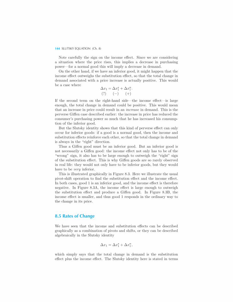
144 SLUTSKY EQUATION (Ch. 8)
Note carefully the sign on the income effect. Since we are consideringa situation where the price rises, this implies a decrease in purchasingpower—for a normal good this will imply a decrease in demand.On the other hand, if we have an inferior good, it might happen that the
income effect outweighs the substitution effect, so that the total change indemand associated with a price increase is actually positive. This wouldbe a case where
Δx1
(?)
= Δxs1
(−)
+ Δxn1 .
(+)
If the second term on the right-hand side—the income effect—is largeenough, the total change in demand could be positive. This would meanthat an increase in price could result in an increase in demand. This is theperverse Giffen case described earlier: the increase in price has reduced theconsumer’s purchasing power so much that he has increased his consump-tion of the inferior good.But the Slutsky identity shows that this kind of perverse effect can only
occur for inferior goods: if a good is a normal good, then the income andsubstitution effects reinforce each other, so that the total change in demandis always in the “right” direction.Thus a Giffen good must be an inferior good. But an inferior good is
not necessarily a Giffen good: the income effect not only has to be of the“wrong” sign, it also has to be large enough to outweigh the “right” signof the substitution effect. This is why Giffen goods are so rarely observedin real life: they would not only have to be inferior goods, but they wouldhave to be very inferior.This is illustrated graphically in Figure 8.3. Here we illustrate the usual
pivot-shift operation to find the substitution effect and the income effect.In both cases, good 1 is an inferior good, and the income effect is thereforenegative. In Figure 8.3A, the income effect is large enough to outweighthe substitution effect and produce a Giffen good. In Figure 8.3B, theincome effect is smaller, and thus good 1 responds in the ordinary way tothe change in its price.
8.5 Rates of Change
We have seen that the income and substitution effects can be describedgraphically as a combination of pivots and shifts, or they can be describedalgebraically in the Slutsky identity
Δx1 = Δxs1 +Δxn
1 ,
which simply says that the total change in demand is the substitutioneffect plus the income effect. The Slutsky identity here is stated in terms
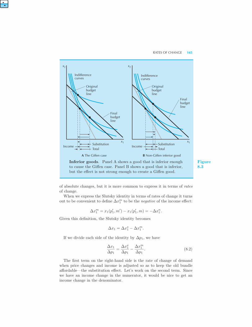
RATES OF CHANGE 145
Income
A The Giffen case
Finalbudgetline
Originalbudgetline
Indifferencecurves
x2
x1
Income
B Non-Giffen inferior good
Finalbudgetline
Originalbudgetline
Indifferencecurves
SubstitutionTotal
SubstitutionTotal
x1
x2
Inferior goods. Panel A shows a good that is inferior enoughto cause the Giffen case. Panel B shows a good that is inferior,but the effect is not strong enough to create a Giffen good.
Figure8.3
of absolute changes, but it is more common to express it in terms of ratesof change.When we express the Slutsky identity in terms of rates of change it turns
out to be convenient to define Δxm1 to be the negative of the income effect:
Δxm1 = x1(p
′1,m
′)− x1(p′1,m) = −Δxn
1 .
Given this definition, the Slutsky identity becomes
Δx1 = Δxs1 −Δxm
1 .
If we divide each side of the identity by Δp1, we have
Δx1
Δp1=
Δxs1
Δp1− Δxm
1
Δp1. (8.2)
The first term on the right-hand side is the rate of change of demandwhen price changes and income is adjusted so as to keep the old bundleaffordable—the substitution effect. Let’s work on the second term. Sincewe have an income change in the numerator, it would be nice to get anincome change in the denominator.
146 SLUTSKY EQUATION (Ch. 8)
Remember that the income change, Δm, and the price change, Δp1, arerelated by the formula
Δm = x1Δp1.
Solving for Δp1 we find
Δp1 =Δm
x1.
Now substitute this expression into the last term in (8.2) to get our finalformula:
Δx1
Δp1=
Δxs1
Δp1− Δxm
1
Δmx1.
This is the Slutsky identity in terms of rates of change. We can interpreteach term as follows:
Δx1
Δp1=
x1(p′1,m)− x1(p1,m)
Δp1
is the rate of change in demand as price changes, holding income fixed;
Δxs1
Δp1=
x1(p′1,m
′)− x1(p1,m)
Δp1
is the rate of change in demand as the price changes, adjusting income soas to keep the old bundle just affordable, that is, the substitution effect;and
Δxm1
Δmx1 =
x1(p′1,m
′)− x1(p′1,m)
m′ −mx1 (8.3)
is the rate of change of demand holding prices fixed and adjusting income,that is, the income effect.
The income effect is itself composed of two pieces: how demand changesas income changes, times the original level of demand. When the pricechanges by Δp1, the change in demand due to the income effect is
Δxm1 =
x1(p′1,m
′)− x1(p′1,m)
Δmx1Δp1.
But this last term, x1Δp1, is just the change in income necessary to keepthe old bundle feasible. That is, x1Δp1 = Δm, so the change in demanddue to the income effect reduces to
Δxm1 =
x1(p′1,m
′)− x1(p′1,m)
ΔmΔm,
just as we had before.
EXAMPLES OF INCOME AND SUBSTITUTION EFFECTS 147
8.6 The Law of Demand
In Chapter 5 we voiced some concerns over the fact that consumer theoryseemed to have no particular content: demand could go up or down when aprice increased, and demand could go up or down when income increased.If a theory doesn’t restrict observed behavior in some fashion it isn’t muchof a theory. A model that is consistent with all behavior has no real content.However, we know that consumer theory does have some content—we’ve
seen that choices generated by an optimizing consumer must satisfy theStrong Axiom of Revealed Preference. Furthermore, we’ve seen that anyprice change can be decomposed into two changes: a substitution effectthat is sure to be negative—opposite the direction of the price change—and an income effect whose sign depends on whether the good is a normalgood or an inferior good.Although consumer theory doesn’t restrict how demand changes when
price changes or how demand changes when income changes, it does re-strict how these two kinds of changes interact. In particular, we have thefollowing.
The Law of Demand. If the demand for a good increases when incomeincreases, then the demand for that good must decrease when its price in-creases.
This follows directly from the Slutsky equation: if the demand increaseswhen income increases, we have a normal good. And if we have a normalgood, then the substitution effect and the income effect reinforce each other,and an increase in price will unambiguously reduce demand.
8.7 Examples of Income and Substitution Effects
Let’s now consider some examples of price changes for particular kinds ofpreferences and decompose the demand changes into the income and thesubstitution effects.We start with the case of perfect complements. The Slutsky decomposi-
tion is illustrated in Figure 8.4. When we pivot the budget line around thechosen point, the optimal choice at the new budget line is the same as atthe old one—this means that the substitution effect is zero. The change indemand is due entirely to the income effect in this case.What about the case of perfect substitutes, illustrated in Figure 8.5?
Here when we tilt the budget line, the demand bundle jumps from thevertical axis to the horizontal axis. There is no shifting left to do! Theentire change in demand is due to the substitution effect in this case.
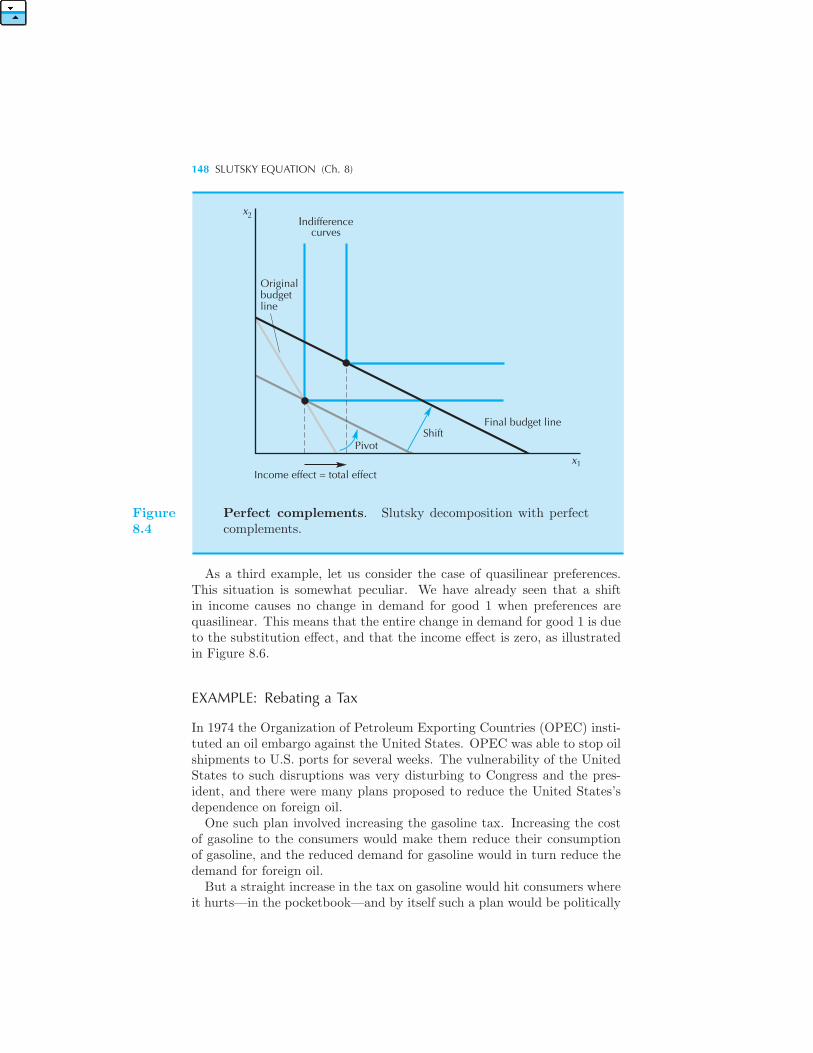
148 SLUTSKY EQUATION (Ch. 8)
Income effect = total effect
PivotShift
Final budget line
Originalbudgetline
Indifferencecurves
x2
x1
Figure8.4
Perfect complements. Slutsky decomposition with perfectcomplements.
As a third example, let us consider the case of quasilinear preferences.This situation is somewhat peculiar. We have already seen that a shiftin income causes no change in demand for good 1 when preferences arequasilinear. This means that the entire change in demand for good 1 is dueto the substitution effect, and that the income effect is zero, as illustratedin Figure 8.6.
EXAMPLE: Rebating a Tax
In 1974 the Organization of Petroleum Exporting Countries (OPEC) insti-tuted an oil embargo against the United States. OPEC was able to stop oilshipments to U.S. ports for several weeks. The vulnerability of the UnitedStates to such disruptions was very disturbing to Congress and the pres-ident, and there were many plans proposed to reduce the United States’sdependence on foreign oil.One such plan involved increasing the gasoline tax. Increasing the cost
of gasoline to the consumers would make them reduce their consumptionof gasoline, and the reduced demand for gasoline would in turn reduce thedemand for foreign oil.But a straight increase in the tax on gasoline would hit consumers where
it hurts—in the pocketbook—and by itself such a plan would be politically
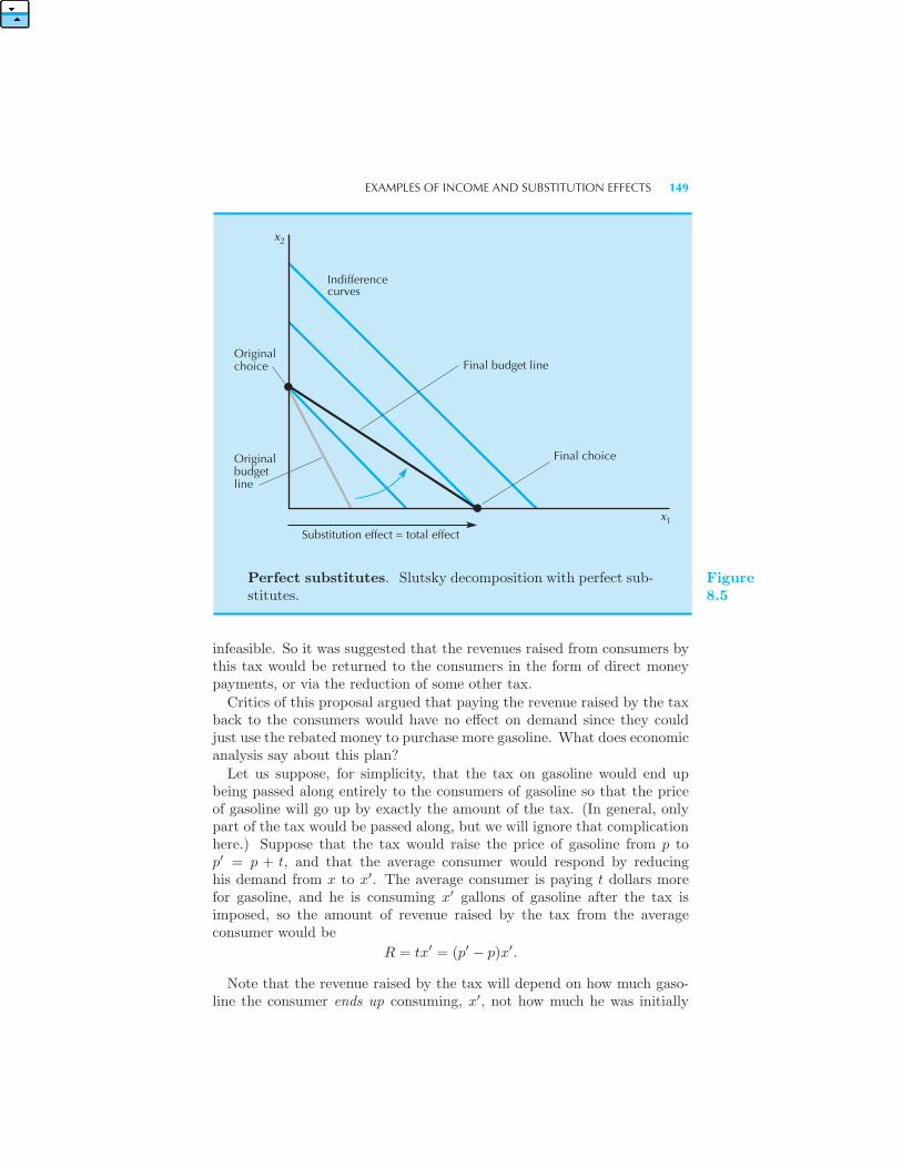
EXAMPLES OF INCOME AND SUBSTITUTION EFFECTS 149
x2
x1
Indifferencecurves
Originalchoice
Originalbudgetline
Final budget line
Final choice
Substitution effect = total effect
Perfect substitutes. Slutsky decomposition with perfect sub-stitutes.
Figure8.5
infeasible. So it was suggested that the revenues raised from consumers bythis tax would be returned to the consumers in the form of direct moneypayments, or via the reduction of some other tax.
Critics of this proposal argued that paying the revenue raised by the taxback to the consumers would have no effect on demand since they couldjust use the rebated money to purchase more gasoline. What does economicanalysis say about this plan?
Let us suppose, for simplicity, that the tax on gasoline would end upbeing passed along entirely to the consumers of gasoline so that the priceof gasoline will go up by exactly the amount of the tax. (In general, onlypart of the tax would be passed along, but we will ignore that complicationhere.) Suppose that the tax would raise the price of gasoline from p top′ = p + t, and that the average consumer would respond by reducinghis demand from x to x′. The average consumer is paying t dollars morefor gasoline, and he is consuming x′ gallons of gasoline after the tax isimposed, so the amount of revenue raised by the tax from the averageconsumer would be
R = tx′ = (p′ − p)x′.
Note that the revenue raised by the tax will depend on how much gaso-line the consumer ends up consuming, x′, not how much he was initially
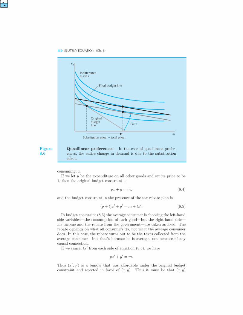
150 SLUTSKY EQUATION (Ch. 8)
Final budget line
x2
Indifference curves
Originalbudgetline
Substitution effect = total effect
Pivot
x1
Figure8.6
Quasilinear preferences. In the case of quasilinear prefer-ences, the entire change in demand is due to the substitutioneffect.
consuming, x.If we let y be the expenditure on all other goods and set its price to be
1, then the original budget constraint is
px+ y = m, (8.4)
and the budget constraint in the presence of the tax-rebate plan is
(p+ t)x′ + y′ = m+ tx′. (8.5)
In budget constraint (8.5) the average consumer is choosing the left-handside variables—the consumption of each good—but the right-hand side—his income and the rebate from the government—are taken as fixed. Therebate depends on what all consumers do, not what the average consumerdoes. In this case, the rebate turns out to be the taxes collected from theaverage consumer—but that’s because he is average, not because of anycausal connection.If we cancel tx′ from each side of equation (8.5), we have
px′ + y′ = m.
Thus (x′, y′) is a bundle that was affordable under the original budgetconstraint and rejected in favor of (x, y). Thus it must be that (x, y)
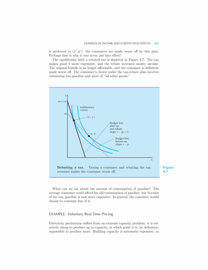
EXAMPLES OF INCOME AND SUBSTITUTION EFFECTS 151
is preferred to (x′, y′): the consumers are made worse off by this plan.Perhaps that is why it was never put into effect!
The equilibrium with a rebated tax is depicted in Figure 8.7. The taxmakes good 1 more expensive, and the rebate increases money income.The original bundle is no longer affordable, and the consumer is definitelymade worse off. The consumer’s choice under the tax-rebate plan involvesconsuming less gasoline and more of “all other goods.”
y
m + tx'
m(x', y' )
(x, y)
Indifferencecurves
Budget lineafter taxand rebateslope = – (p + t )
Budget linebefore taxslope = – p
x
Rebating a tax. Taxing a consumer and rebating the taxrevenues makes the consumer worse off.
Figure8.7
What can we say about the amount of consumption of gasoline? Theaverage consumer could afford his old consumption of gasoline, but becauseof the tax, gasoline is now more expensive. In general, the consumer wouldchoose to consume less of it.
EXAMPLE: Voluntary Real Time Pricing
Electricity production suffers from an extreme capacity problem: it is rel-atively cheap to produce up to capacity, at which point it is, by definition,impossible to produce more. Building capacity is extremely expensive, so
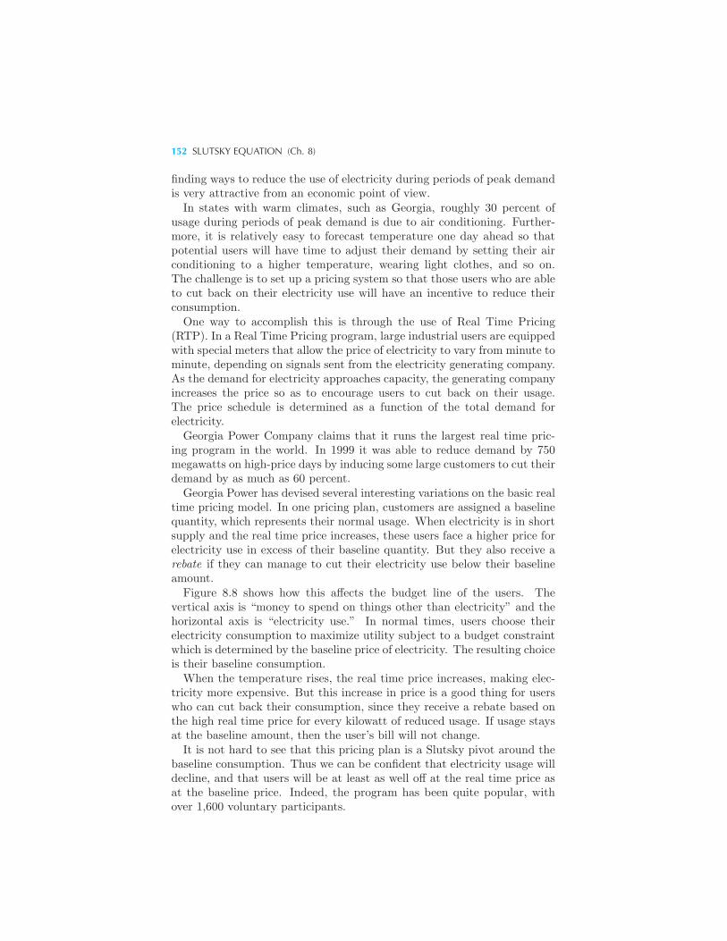
152 SLUTSKY EQUATION (Ch. 8)
finding ways to reduce the use of electricity during periods of peak demandis very attractive from an economic point of view.In states with warm climates, such as Georgia, roughly 30 percent of
usage during periods of peak demand is due to air conditioning. Further-more, it is relatively easy to forecast temperature one day ahead so thatpotential users will have time to adjust their demand by setting their airconditioning to a higher temperature, wearing light clothes, and so on.The challenge is to set up a pricing system so that those users who are ableto cut back on their electricity use will have an incentive to reduce theirconsumption.One way to accomplish this is through the use of Real Time Pricing
(RTP). In a Real Time Pricing program, large industrial users are equippedwith special meters that allow the price of electricity to vary from minute tominute, depending on signals sent from the electricity generating company.As the demand for electricity approaches capacity, the generating companyincreases the price so as to encourage users to cut back on their usage.The price schedule is determined as a function of the total demand forelectricity.Georgia Power Company claims that it runs the largest real time pric-
ing program in the world. In 1999 it was able to reduce demand by 750megawatts on high-price days by inducing some large customers to cut theirdemand by as much as 60 percent.Georgia Power has devised several interesting variations on the basic real
time pricing model. In one pricing plan, customers are assigned a baselinequantity, which represents their normal usage. When electricity is in shortsupply and the real time price increases, these users face a higher price forelectricity use in excess of their baseline quantity. But they also receive arebate if they can manage to cut their electricity use below their baselineamount.Figure 8.8 shows how this affects the budget line of the users. The
vertical axis is “money to spend on things other than electricity” and thehorizontal axis is “electricity use.” In normal times, users choose theirelectricity consumption to maximize utility subject to a budget constraintwhich is determined by the baseline price of electricity. The resulting choiceis their baseline consumption.When the temperature rises, the real time price increases, making elec-
tricity more expensive. But this increase in price is a good thing for userswho can cut back their consumption, since they receive a rebate based onthe high real time price for every kilowatt of reduced usage. If usage staysat the baseline amount, then the user’s bill will not change.It is not hard to see that this pricing plan is a Slutsky pivot around the
baseline consumption. Thus we can be confident that electricity usage willdecline, and that users will be at least as well off at the real time price asat the baseline price. Indeed, the program has been quite popular, withover 1,600 voluntary participants.
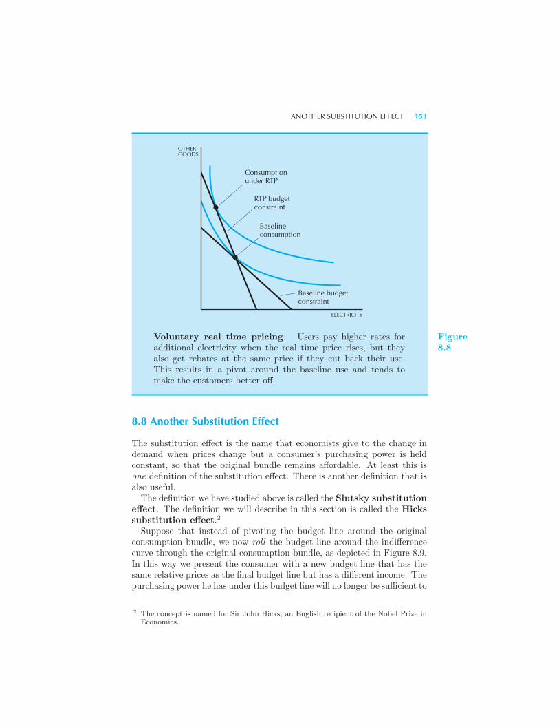
ANOTHER SUBSTITUTION EFFECT 153
Baselineconsumption
OTHERGOODS
ELECTRICITY
Baseline budgetconstraint
RTP budgetconstraint
Consumptionunder RTP
Voluntary real time pricing. Users pay higher rates foradditional electricity when the real time price rises, but theyalso get rebates at the same price if they cut back their use.This results in a pivot around the baseline use and tends tomake the customers better off.
Figure8.8
8.8 Another Substitution Effect
The substitution effect is the name that economists give to the change indemand when prices change but a consumer’s purchasing power is heldconstant, so that the original bundle remains affordable. At least this isone definition of the substitution effect. There is another definition that isalso useful.The definition we have studied above is called the Slutsky substitution
effect. The definition we will describe in this section is called the Hickssubstitution effect.2
Suppose that instead of pivoting the budget line around the originalconsumption bundle, we now roll the budget line around the indifferencecurve through the original consumption bundle, as depicted in Figure 8.9.In this way we present the consumer with a new budget line that has thesame relative prices as the final budget line but has a different income. Thepurchasing power he has under this budget line will no longer be sufficient to
2 The concept is named for Sir John Hicks, an English recipient of the Nobel Prize inEconomics.
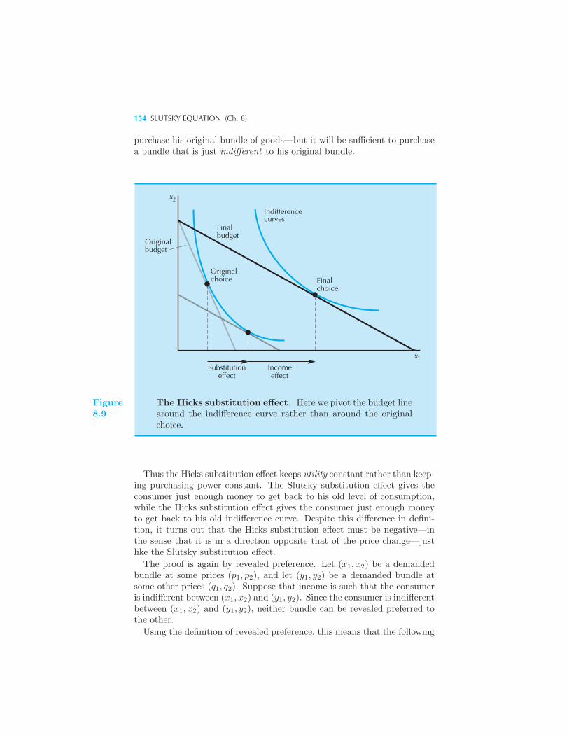
154 SLUTSKY EQUATION (Ch. 8)
purchase his original bundle of goods—but it will be sufficient to purchasea bundle that is just indifferent to his original bundle.
x
x1
2
Finalbudget
Indifferencecurves
Finalchoice
Originalchoice
Originalbudget
Substitutioneffect
Incomeeffect
Figure8.9
The Hicks substitution effect. Here we pivot the budget linearound the indifference curve rather than around the originalchoice.
Thus the Hicks substitution effect keeps utility constant rather than keep-ing purchasing power constant. The Slutsky substitution effect gives theconsumer just enough money to get back to his old level of consumption,while the Hicks substitution effect gives the consumer just enough moneyto get back to his old indifference curve. Despite this difference in defini-tion, it turns out that the Hicks substitution effect must be negative—inthe sense that it is in a direction opposite that of the price change—justlike the Slutsky substitution effect.
The proof is again by revealed preference. Let (x1, x2) be a demandedbundle at some prices (p1, p2), and let (y1, y2) be a demanded bundle atsome other prices (q1, q2). Suppose that income is such that the consumeris indifferent between (x1, x2) and (y1, y2). Since the consumer is indifferentbetween (x1, x2) and (y1, y2), neither bundle can be revealed preferred tothe other.
Using the definition of revealed preference, this means that the following
COMPENSATED DEMAND CURVES 155
two inequalities are not true:
p1x1 + p2x2 > p1y1 + p2y2
q1y1 + q2y2 > q1x1 + q2x2.
It follows that these inequalities are true:
p1x1 + p2x2 ≤ p1y1 + p2y2
q1y1 + q2y2 ≤ q1x1 + q2x2.
Adding these inequalities together and rearranging them we have
(q1 − p1)(y1 − x1) + (q2 − p2)(y2 − x2) ≤ 0.
This is a general statement about how demands change when priceschange if income is adjusted so as to keep the consumer on the same in-difference curve. In the particular case we are concerned with, we are onlychanging the first price. Therefore q2 = p2, and we are left with
(q1 − p1)(y1 − x1) ≤ 0.
This equation says that the change in the quantity demanded must havethe opposite sign from that of the price change, which is what we wantedto show.The total change in demand is still equal to the substitution effect plus
the income effect—but now it is the Hicks substitution effect. Since theHicks substitution effect is also negative, the Slutsky equation takes exactlythe same form as we had earlier and has exactly the same interpretation.Both the Slutsky and Hicks definitions of the substitution effect have theirplace, and which is more useful depends on the problem at hand. It canbe shown that for small changes in price, the two substitution effects arevirtually identical.
8.9 Compensated Demand Curves
We have seen how the quantity demanded changes as a price changes inthree different contexts: holding income fixed (the standard case), holdingpurchasing power fixed (the Slutsky substitution effect), and holding utilityfixed (the Hicks substitution effect). We can draw the relationship betweenprice and quantity demanded holding any of these three variables fixed.This gives rise to three different demand curves: the standard demandcurve, the Slutsky demand curve, and the Hicks demand curve.The analysis of this chapter shows that the Slutsky and Hicks demand
curves are always downward sloping curves. Furthermore the ordinary
156 SLUTSKY EQUATION (Ch. 8)
demand curve is a downward sloping curve for normal goods. However,the Giffen analysis shows that it is theoretically possible that the ordinarydemand curve may slope upwards for an inferior good.
The Hicksian demand curve—the one with utility held constant—is some-times called the compensated demand curve. This terminology arisesnaturally if you think of constructing the Hicksian demand curve by ad-justing income as the price changes so as to keep the consumer’s utilityconstant. Hence the consumer is “compensated” for the price changes, andhis utility is the same at every point on the Hicksian demand curve. Thisis in contrast to the situation with an ordinary demand curve. In this casethe consumer is worse off facing higher prices than lower prices since hisincome is constant.
The compensated demand curve turns out to be very useful in advancedcourses, especially in treatments of benefit-cost analysis. In this sort ofanalysis it is natural to ask what size payments are necessary to compen-sate consumers for some policy change. The magnitude of such paymentsgives a useful estimate of the cost of the policy change. However, actualcalculation of compensated demand curves requires more mathematical ma-chinery than we have developed in this text.
Summary
1. When the price of a good decreases, there will be two effects on consump-tion. The change in relative prices makes the consumer want to consumemore of the cheaper good. The increase in purchasing power due to thelower price may increase or decrease consumption, depending on whetherthe good is a normal good or an inferior good.
2. The change in demand due to the change in relative prices is called thesubstitution effect; the change due to the change in purchasing power iscalled the income effect.
3. The substitution effect is how demand changes when prices change andpurchasing power is held constant, in the sense that the original bundleremains affordable. To hold real purchasing power constant, money incomewill have to change. The necessary change in money income is given byΔm = x1Δp1.
4. The Slutsky equation says that the total change in demand is the sumof the substitution effect and the income effect.
5. The Law of Demand says that normal goods must have downward-sloping demand curves.
APPENDIX 157
REVIEW QUESTIONS
1. Suppose a consumer has preferences between two goods that are perfectsubstitutes. Can you change prices in such a way that the entire demandresponse is due to the income effect?
2. Suppose that preferences are concave. Is it still the case that the substi-tution effect is negative?
3. In the case of the gasoline tax, what would happen if the rebate to theconsumers were based on their original consumption of gasoline, x, ratherthan on their final consumption of gasoline, x′?
4. In the case described in the preceding question, would the governmentbe paying out more or less than it received in tax revenues?
5. In this case would the consumers be better off or worse off if the taxwith rebate based on original consumption were in effect?
APPENDIX
Let us derive the Slutsky equation using calculus. Consider the Slutsky defini-tion of the substitution effect, in which the income is adjusted so as to give theconsumer just enough to buy the original consumption bundle, which we will nowdenote by (x1, x2). If the prices are (p1, p2), then the consumer’s actual choicewith this adjustment will depend on (p1, p2) and (x1, x2). Let’s call this relation-ship the Slutsky demand function for good 1, and write it as xs
1(p1, p2, x1, x2).Suppose the original demanded bundle is (x1, x2) at prices (p1, p2) and income
m. The Slutsky demand function tells us what the consumer would demandfacing some different prices (p1, p2) and having income p1x1 + p2x2. Thus theSlutsky demand function at (p1, p2, x1, x2) is the ordinary demand at (p1, p2) andincome p1x1 + p2x2. That is,
xs1(p1, p2, x1, x2) ≡ x1(p1, p2, p1x1 + p2x2).
This equation says that the Slutsky demand at prices (p1, p2) is that amountwhich the consumer would demand if he had enough income to purchase hisoriginal bundle of goods (x1, x2). This is just the definition of the Slutsky demandfunction.
Differentiating this identity with respect to p1, we have
∂xs1(p1, p2, x1, x2)
∂p1=
∂x1(p1, p2,m)
∂p1+
∂x1(p1, p2,m)
∂mx1.
Rearranging we have
∂x1(p1, p2,m)
∂p1=
∂xs1(p1, p2, x1, x2)
∂p1− ∂x1(p1, p2,m)
∂mx1.
158 SLUTSKY EQUATION (Ch. 8)
Note the use of the chain rule in this calculation.This is a derivative form of the Slutsky equation. It says that the total effect
of a price change is composed of a substitution effect (where income is adjustedto keep the bundle (x1, x2) feasible) and an income effect. We know from thetext that the substitution effect is negative and that the sign of the income effectdepends on whether the good in question is inferior or not. As you can see, thisis just the form of the Slutsky equation considered in the text, except that wehave replaced the Δ’s with derivative signs.
What about the Hicks substitution effect? It is also possible to define a Slutskyequation for it. We let xh
1 (p1, p2, u) be the Hicksian demand function, whichmeasures how much the consumer demands of good 1 at prices (p1, p2) if incomeis adjusted to keep the level of utility constant at the original level u. It turnsout that in this case the Slutsky equation takes the form
∂x1(p1, p2,m)
∂p1=
∂xh1 (p1, p2, u)
∂p1− ∂x1(p1, p2,m)
∂mx1.
The proof of this equation hinges on the fact that
∂xh1 (p1, p2, u)
∂p1=
∂xs1(p1, p2, x1, x2)
∂p1
for infinitesimal changes in price. That is, for derivative size changes in price, theSlutsky substitution and the Hicks substitution effect are the same. The proofof this is not terribly difficult, but it involves some concepts that are beyondthe scope of this book. A relatively simple proof is given in Hal R. Varian,Microeconomic Analysis, 3rd ed. (New York: Norton, 1992).
EXAMPLE: Rebating a Small Tax
We can use the calculus version of the Slutsky equation to see how consumptionchoices would react to a small change in a tax when the tax revenues are rebatedto the consumers.
Assume, as before, that the tax causes the price to rise by the full amount ofthe tax. Let x be the amount of gasoline, p its original price, and t the amountof the tax. Then the change in consumption will be given by
dx =∂x
∂pt+
∂x
∂mtx.
The first term measures how demand responds to the price change times theamount of the price change—which gives us the price effect of the tax. Thesecond terms tells us how demand responds to a change in income times theamount that income has changed—income has gone up by the amount of the taxrevenues rebated to the consumer.
Now use Slutsky’s equation to expand the first term on the right-hand side toget the substitution and income effects of the price change itself:
dx =∂xs
∂pt− ∂x
∂mtx+
∂x
∂mtx =
∂xs
∂pt.
APPENDIX 159
The income effect cancels out, and all that is left is the pure substitution effect.Imposing a small tax and rebating the revenues of the tax is just like impos-ing a price change and adjusting income so that the old consumption bundle isfeasible—as long as the tax is small enough so that the derivative approximationis valid.
CHAPTER 9
BUYING ANDSELLING
In the simple model of the consumer that we considered in the precedingchapters, the income of the consumer was given. In reality people earn theirincome by selling things that they own: items that they have produced,assets that they have accumulated, or, most commonly, their own labor.In this chapter we will examine how the earlier model must be modified soas to describe this kind of behavior.
9.1 Net and Gross Demands
As before, we will limit ourselves to the two-good model. We now sup-pose that the consumer starts off with an endowment of the two goods,which we will denote by (ω1, ω2).
1 This is how much of the two goods theconsumer has before he enters the market. Think of a farmer who goesto market with ω1 units of carrots and ω2 units of potatoes. The farmerinspects the prices available at the market and decides how much he wantsto buy and sell of the two goods.
1 The Greek letter ω, omega, is pronounced “o–may–gah.”
THE BUDGET CONSTRAINT 161
Let us make a distinction here between the consumer’s gross demandsand his net demands. The gross demand for a good is the amount of thegood that the consumer actually ends up consuming: how much of each ofthe goods he or she takes home from the market. The net demand for agood is the difference between what the consumer ends up with (the grossdemand) and the initial endowment of goods. The net demand for a goodis simply the amount that is bought or sold of the good.If we let (x1, x2) be the gross demands, then (x1 − ω1, x2 − ω2) are the
net demands. Note that while the gross demands are typically positivenumbers, the net demands may be positive or negative. If the net demandfor good 1 is negative, it means that the consumer wants to consume lessof good 1 than she has; that is, she wants to supply good 1 to the market.A negative net demand is simply an amount supplied.For purposes of economic analysis, the gross demands are the more im-
portant, since that is what the consumer is ultimately concerned with. Butthe net demands are what are actually exhibited in the market and thusare closer to what the layman means by demand or supply.
9.2 The Budget Constraint
The first thing we should do is to consider the form of the budget constraint.What constrains the consumer’s final consumption? It must be that thevalue of the bundle of goods that she goes home with must be equal to thevalue of the bundle of goods that she came with. Or, algebraically:
p1x1 + p2x2 = p1ω1 + p2ω2.
We could just as well express this budget line in terms of net demands as
p1(x1 − ω1) + p2(x2 − ω2) = 0.
If (x1 − ω1) is positive we say that the consumer is a net buyer or netdemander of good 1; if it is negative we say that she is a net seller ornet supplier. Then the above equation says that the value of what theconsumer buys must equal the value of what she sells, which seems sensibleenough.We could also express the budget line when the endowment is present
in a form similar to the way we described it before. Now it takes twoequations:
p1x1 + p2x2 = m
m = p1ω1 + p2ω2.
Once the prices are fixed, the value of the endowment, and hence theconsumer’s money income, is fixed.
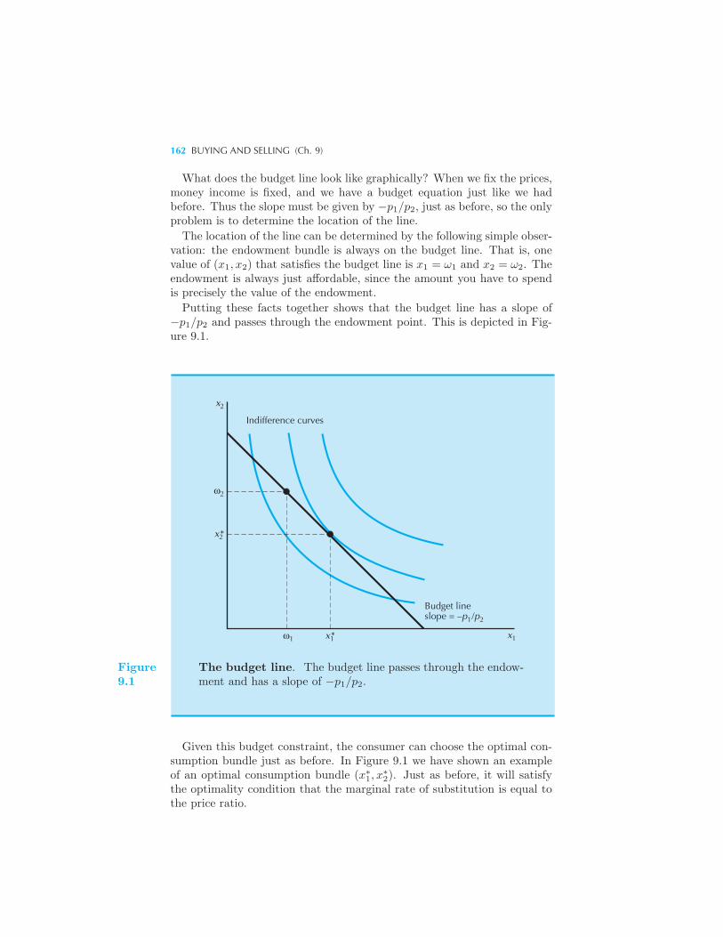
162 BUYING AND SELLING (Ch. 9)
What does the budget line look like graphically? When we fix the prices,money income is fixed, and we have a budget equation just like we hadbefore. Thus the slope must be given by −p1/p2, just as before, so the onlyproblem is to determine the location of the line.
The location of the line can be determined by the following simple obser-vation: the endowment bundle is always on the budget line. That is, onevalue of (x1, x2) that satisfies the budget line is x1 = ω1 and x2 = ω2. Theendowment is always just affordable, since the amount you have to spendis precisely the value of the endowment.
Putting these facts together shows that the budget line has a slope of−p1/p2 and passes through the endowment point. This is depicted in Fig-ure 9.1.
Indifference curves
x
x*
ω2
2
2
1 1x*ω
Budget lineslope = –p /p
x1
1 2
Figure9.1
The budget line. The budget line passes through the endow-ment and has a slope of −p1/p2.
Given this budget constraint, the consumer can choose the optimal con-sumption bundle just as before. In Figure 9.1 we have shown an exampleof an optimal consumption bundle (x∗
1, x∗2). Just as before, it will satisfy
the optimality condition that the marginal rate of substitution is equal tothe price ratio.
CHANGING THE ENDOWMENT 163
In this particular case, x∗1 > ω1 and x∗
2 < ω2, so the consumer is a netbuyer of good 1 and a net seller of good 2. The net demands are simply thenet amounts that the consumer buys or sells of the two goods. In generalthe consumer may decide to be either a buyer or a seller depending on therelative prices of the two goods.
9.3 Changing the Endowment
In our previous analysis of choice we examined how the optimal consump-tion changed as the money income changed while the prices remained fixed.We can do a similar analysis here by asking how the optimal consumptionchanges as the endowment changes while the prices remain fixed.For example, suppose that the endowment changes from (ω1, ω2) to some
other value (ω′1, ω
′2) such that
p1ω1 + p2ω2 > p1ω′1 + p2ω
′2.
This inequality means that the new endowment (ω′1, ω
′2) is worth less than
the old endowment—the money income that the consumer could achieveby selling her endowment is less.This is depicted graphically in Figure 9.2A: the budget line shifts in-
ward. Since this is exactly the same as a reduction in money income, wecan conclude the same two things that we concluded in our examination ofthat case. First, the consumer is definitely worse off with the endowment(ω′
1, ω′2) than she was with the old endowment, since her consumption pos-
sibilities have been reduced. Second, her demand for each good will changeaccording to whether that good is a normal good or an inferior good.For example, if good 1 is a normal good and the consumer’s endowment
changes in a way that reduces its value, we can conclude that the consumer’sdemand for good 1 will decrease.The case where the value of the endowment increases is depicted in Fig-
ure 9.2B. Following the above argument we conclude that if the budgetline shifts outward in a parallel way, the consumer must be made betteroff. Algebraically, if the endowment changes from (ω1, ω2) to (ω′
1, ω′2) and
p1ω1 + p2ω2 < p1ω′1 + p2ω
′2, then the consumer’s new budget set must con-
tain her old budget set. This in turn implies that the optimal choice of theconsumer with the new budget set must be preferred to the optimal choicegiven the old endowment.It is worthwhile pondering this point a moment. In Chapter 7 we argued
that just because a consumption bundle had a higher cost than anotherdidn’t mean that it would be preferred to the other bundle. But thatonly holds for a bundle that must be consumed. If a consumer can sell abundle of goods on a free market at constant prices, then she will alwaysprefer a higher-valued bundle to a lower-valued bundle, simply because a
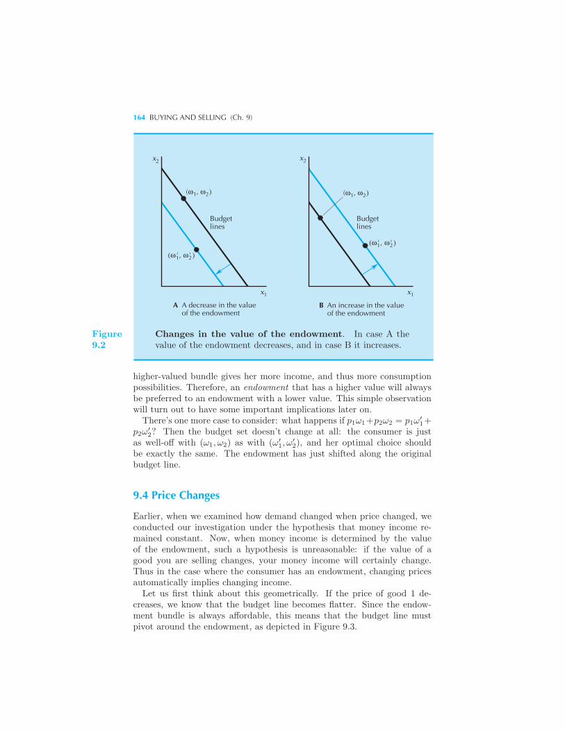
164 BUYING AND SELLING (Ch. 9)
xx
x x
Budgetlines
Budgetlines
1 1
22
1 2
1 2
A A decrease in the value of the endowment
B An increase in the value of the endowment
(ω , ω )
(ω' , ω' )
1 2(ω , ω )
1 2(ω' , ω' )
Figure9.2
Changes in the value of the endowment. In case A thevalue of the endowment decreases, and in case B it increases.
higher-valued bundle gives her more income, and thus more consumptionpossibilities. Therefore, an endowment that has a higher value will alwaysbe preferred to an endowment with a lower value. This simple observationwill turn out to have some important implications later on.There’s one more case to consider: what happens if p1ω1+p2ω2 = p1ω
′1+
p2ω′2? Then the budget set doesn’t change at all: the consumer is just
as well-off with (ω1, ω2) as with (ω′1, ω
′2), and her optimal choice should
be exactly the same. The endowment has just shifted along the originalbudget line.
9.4 Price Changes
Earlier, when we examined how demand changed when price changed, weconducted our investigation under the hypothesis that money income re-mained constant. Now, when money income is determined by the valueof the endowment, such a hypothesis is unreasonable: if the value of agood you are selling changes, your money income will certainly change.Thus in the case where the consumer has an endowment, changing pricesautomatically implies changing income.Let us first think about this geometrically. If the price of good 1 de-
creases, we know that the budget line becomes flatter. Since the endow-ment bundle is always affordable, this means that the budget line mustpivot around the endowment, as depicted in Figure 9.3.
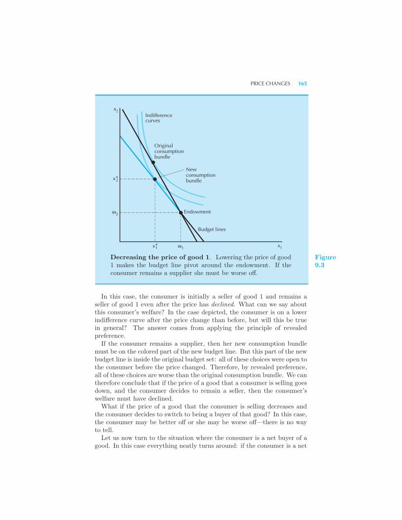
PRICE CHANGES 165
x*2
2
2ω
*1x 1ω 1x
Budget lines
Endowment
New consumptionbundle
Originalconsumptionbundle
Indifferencecurves
x
Decreasing the price of good 1. Lowering the price of good1 makes the budget line pivot around the endowment. If theconsumer remains a supplier she must be worse off.
Figure9.3
In this case, the consumer is initially a seller of good 1 and remains aseller of good 1 even after the price has declined. What can we say aboutthis consumer’s welfare? In the case depicted, the consumer is on a lowerindifference curve after the price change than before, but will this be truein general? The answer comes from applying the principle of revealedpreference.If the consumer remains a supplier, then her new consumption bundle
must be on the colored part of the new budget line. But this part of the newbudget line is inside the original budget set: all of these choices were open tothe consumer before the price changed. Therefore, by revealed preference,all of these choices are worse than the original consumption bundle. We cantherefore conclude that if the price of a good that a consumer is selling goesdown, and the consumer decides to remain a seller, then the consumer’swelfare must have declined.What if the price of a good that the consumer is selling decreases and
the consumer decides to switch to being a buyer of that good? In this case,the consumer may be better off or she may be worse off—there is no wayto tell.Let us now turn to the situation where the consumer is a net buyer of a
good. In this case everything neatly turns around: if the consumer is a net
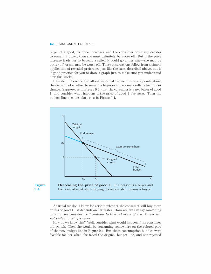
166 BUYING AND SELLING (Ch. 9)
buyer of a good, its price increases, and the consumer optimally decidesto remain a buyer, then she must definitely be worse off. But if the priceincrease leads her to become a seller, it could go either way—she may bebetter off, or she may be worse off. These observations follow from a simpleapplication of revealed preference just like the cases described above, but itis good practice for you to draw a graph just to make sure you understandhow this works.Revealed preference also allows us to make some interesting points about
the decision of whether to remain a buyer or to become a seller when priceschange. Suppose, as in Figure 9.4, that the consumer is a net buyer of good1, and consider what happens if the price of good 1 decreases. Then thebudget line becomes flatter as in Figure 9.4.
ω
ω xx*
x*
x
Originalbudget
Endowment
Must consume here
Originalchoice
Newbudget
1 1 1
2
2
2
Figure9.4
Decreasing the price of good 1. If a person is a buyer andthe price of what she is buying decreases, she remains a buyer.
As usual we don’t know for certain whether the consumer will buy moreor less of good 1—it depends on her tastes. However, we can say somethingfor sure: the consumer will continue to be a net buyer of good 1—she willnot switch to being a seller.How do we know this? Well, consider what would happen if the consumer
did switch. Then she would be consuming somewhere on the colored partof the new budget line in Figure 9.4. But those consumption bundles werefeasible for her when she faced the original budget line, and she rejected
OFFER CURVES AND DEMAND CURVES 167
them in favor of (x∗1, x
∗2). So (x∗
1, x∗2) must be better than any of those
points. And under the new budget line, (x∗1, x
∗2) is a feasible consumption
bundle. So whatever she consumes under the new budget line, it must bebetter than (x∗
1, x∗2)—and thus better than any points on the colored part
of the new budget line. This implies that her consumption of x1 mustbe to the right of her endowment point—that is, she must remain a netdemander of good 1.Again, this kind of observation applies equally well to a person who is
a net seller of a good: if the price of what she is selling goes up, she willnot switch to being a net buyer. We can’t tell for sure if the consumer willconsume more or less of the good she is selling—but we know that she willkeep selling it if the price goes up.
9.5 Offer Curves and Demand Curves
Recall from Chapter 6 that price offer curves depict those combinations ofboth goods that may be demanded by a consumer and that demand curvesdepict the relationship between the price and the quantity demanded ofsome good. Exactly the same constructions work when the consumer hasan endowment of both goods.Consider, for example, Figure 9.5, which illustrates the price offer curve
and the demand curve for a consumer. The offer curve will always passthrough the endowment, because at some price the endowment will bea demanded bundle; that is, at some prices the consumer will optimallychoose not to trade.As we’ve seen, the consumer may decide to be a buyer of good 1 for
some prices and a seller of good 1 for other prices. Thus the offer curvewill generally pass to the left and to the right of the endowment point.The demand curve illustrated in Figure 9.5B is the gross demand curve—
it measures the total amount the consumer chooses to consume of good 1.We have illustrated the net demand curve in Figure 9.6.Note that the net demand for good 1 will typically be negative for some
prices. This will be when the price of good 1 becomes so high that theconsumer chooses to become a seller of good 1. At some price the consumerswitches between being a net demander to being a net supplier of good 1.It is conventional to plot the supply curve in the positive orthant, al-
though it actually makes more sense to think of supply as just a negativedemand. We’ll bow to tradition here and plot the net supply curve in thenormal way—as a positive amount, as in Figure 9.6.Algebraically the net demand for good 1, d1(p1, p2), is the difference
between the gross demand x1(p1, p2) and the endowment of good 1, whenthis difference is positive; that is, when the consumer wants more of thegood than he or she has:
d1(p1, p2) ={x1(p1, p2)− ω1 if this is positive;0 otherwise.
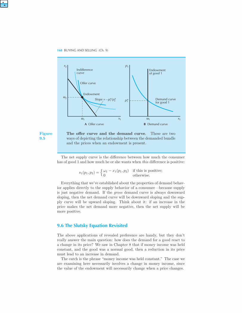
168 BUYING AND SELLING (Ch. 9)
Indifferencecurve
Offer curve
Endowment
Slope = –p*/p*
x p
p*
x x1 1 1
1
1
1
2
2
A Offer curve B Demand curve
ω
ω ω
Demand curvefor good 1
Endowmentof good 1
1 2
Figure9.5
The offer curve and the demand curve. These are twoways of depicting the relationship between the demanded bundleand the prices when an endowment is present.
The net supply curve is the difference between how much the consumerhas of good 1 and how much he or she wants when this difference is positive:
s1(p1, p2) ={ω1 − x1(p1, p2) if this is positive;0 otherwise.
Everything that we’ve established about the properties of demand behav-ior applies directly to the supply behavior of a consumer—because supplyis just negative demand. If the gross demand curve is always downwardsloping, then the net demand curve will be downward sloping and the sup-ply curve will be upward sloping. Think about it: if an increase in theprice makes the net demand more negative, then the net supply will bemore positive.
9.6 The Slutsky Equation Revisited
The above applications of revealed preference are handy, but they don’treally answer the main question: how does the demand for a good react toa change in its price? We saw in Chapter 8 that if money income was heldconstant, and the good was a normal good, then a reduction in its pricemust lead to an increase in demand.The catch is the phrase “money income was held constant.” The case we
are examining here necessarily involves a change in money income, sincethe value of the endowment will necessarily change when a price changes.
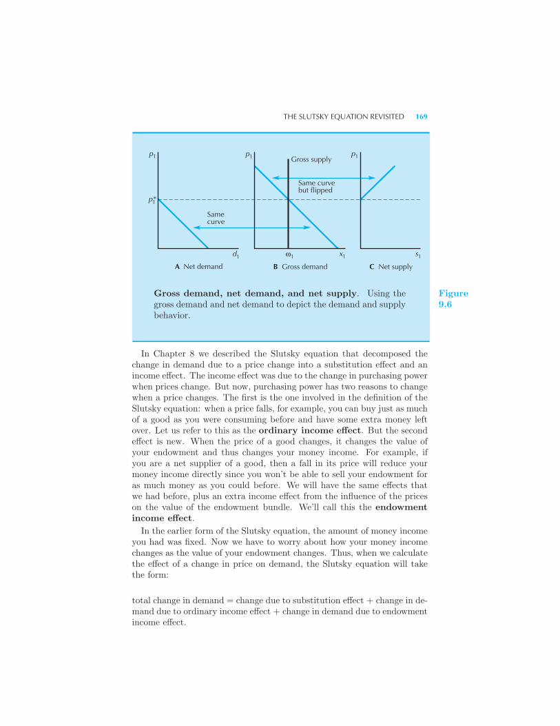
THE SLUTSKY EQUATION REVISITED 169
p11p1p
1p*
Samecurve
d s1111
A Net demand B Gross demand C Net supply
Gross supply
Same curvebut flipped
ω x
Gross demand, net demand, and net supply. Using thegross demand and net demand to depict the demand and supplybehavior.
Figure9.6
In Chapter 8 we described the Slutsky equation that decomposed thechange in demand due to a price change into a substitution effect and anincome effect. The income effect was due to the change in purchasing powerwhen prices change. But now, purchasing power has two reasons to changewhen a price changes. The first is the one involved in the definition of theSlutsky equation: when a price falls, for example, you can buy just as muchof a good as you were consuming before and have some extra money leftover. Let us refer to this as the ordinary income effect. But the secondeffect is new. When the price of a good changes, it changes the value ofyour endowment and thus changes your money income. For example, ifyou are a net supplier of a good, then a fall in its price will reduce yourmoney income directly since you won’t be able to sell your endowment foras much money as you could before. We will have the same effects thatwe had before, plus an extra income effect from the influence of the priceson the value of the endowment bundle. We’ll call this the endowmentincome effect.
In the earlier form of the Slutsky equation, the amount of money incomeyou had was fixed. Now we have to worry about how your money incomechanges as the value of your endowment changes. Thus, when we calculatethe effect of a change in price on demand, the Slutsky equation will takethe form:
total change in demand = change due to substitution effect + change in de-mand due to ordinary income effect + change in demand due to endowmentincome effect.
170 BUYING AND SELLING (Ch. 9)
The first two effects are familiar. As before, let us use Δx1 to stand forthe total change in demand, Δxs
1 to stand for the change in demand dueto the substitution effect, and Δxm
1 to stand for the change in demand dueto the ordinary income effect. Then we can substitute these terms into theabove “verbal equation” to get the Slutsky equation in terms of rates ofchange:
Δx1
Δp1=
Δxs1
Δp1− x1
Δxm1
Δm+ endowment income effect. (9.1)
What will the last term look like? We’ll derive an explicit expressionbelow, but let us first think about what is involved. When the price of theendowment changes, money income will change, and this change in moneyincome will induce a change in demand. Thus the endowment income effectwill consist of two terms:
endowment income effect = change in demand when income changes× the change in income when price changes. (9.2)
Let’s look at the second effect first. Since income is defined to be
m = p1ω1 + p2ω2,
we haveΔm
Δp1= ω1.
This tells us how money income changes when the price of good 1 changes:if you have 10 units of good 1 to sell, and its price goes up by $1, yourmoney income will go up by $10.The first term in equation (9.2) is just how demand changes when income
changes. We already have an expression for this: it is Δxm1 /Δm: the change
in demand divided by the change in income. Thus the endowment incomeeffect is given by
endowment income effect =Δxm
1
Δm
Δm
Δp1=
Δxm1
Δmω1. (9.3)
Inserting equation (9.3) into equation (9.1) we get the final form of theSlutsky equation:
Δx1
Δp1=
Δxs1
Δp1+ (ω1 − x1)
Δxm1
Δm.
This equation can be used to answer the question posed above. We knowthat the sign of the substitution effect is always negative—opposite thedirection of the change in price. Let us suppose that the good is a normal
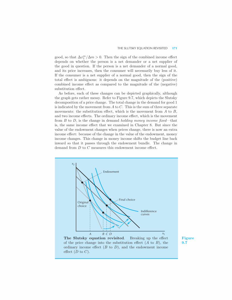
THE SLUTSKY EQUATION REVISITED 171
good, so that Δxm1 /Δm > 0. Then the sign of the combined income effect
depends on whether the person is a net demander or a net supplier ofthe good in question. If the person is a net demander of a normal good,and its price increases, then the consumer will necessarily buy less of it.If the consumer is a net supplier of a normal good, then the sign of thetotal effect is ambiguous: it depends on the magnitude of the (positive)combined income effect as compared to the magnitude of the (negative)substitution effect.As before, each of these changes can be depicted graphically, although
the graph gets rather messy. Refer to Figure 9.7, which depicts the Slutskydecomposition of a price change. The total change in the demand for good 1is indicated by the movement from A to C. This is the sum of three separatemovements: the substitution effect, which is the movement from A to B,and two income effects. The ordinary income effect, which is the movementfrom B to D, is the change in demand holding money income fixed—thatis, the same income effect that we examined in Chapter 8. But since thevalue of the endowment changes when prices change, there is now an extraincome effect: because of the change in the value of the endowment, moneyincome changes. This change in money income shifts the budget line backinward so that it passes through the endowment bundle. The change indemand from D to C measures this endowment income effect.
x2
x1A B C D
Originalchoice
Endowment
Final choice
Indifferencecurves
The Slutsky equation revisited. Breaking up the effectof the price change into the substitution effect (A to B), theordinary income effect (B to D), and the endowment incomeeffect (D to C).
Figure9.7
172 BUYING AND SELLING (Ch. 9)
9.7 Use of the Slutsky Equation
Suppose that we have a consumer who sells apples and oranges that hegrows on a few trees in his backyard, like the consumer we described at thebeginning of Chapter 8. We said there that if the price of apples increased,then this consumer might actually consume more apples. Using the Slutskyequation derived in this chapter, it is not hard to see why. If we let xa standfor the consumer’s demand for apples, and let pa be the price of apples,then we know that
ΔxaΔpa
=Δxs
aΔpa(−)
+ (ωa − xa)
(+)
Δxma
Δm .
(+)
This says that the total change in the demand for apples when the priceof apples changes is the substitution effect plus the income effect. The sub-stitution effect works in the right direction—increasing the price decreasesthe demand for apples. But if apples are a normal good for this consumer,the income effect works in the wrong direction. Since the consumer is a netsupplier of apples, the increase in the price of apples increases his moneyincome so much that he wants to consume more apples due to the incomeeffect. If the latter term is strong enough to outweigh the substitutioneffect, we can easily get the “perverse” result.
EXAMPLE: Calculating the Endowment Income Effect
Let’s try a little numerical example. Suppose that a dairy farmer produces40 quarts of milk a week. Initially the price of milk is $3 a quart. Hisdemand function for milk, for his own consumption, is
x1 = 10 +m
10p1.
Since he is producing 40 quarts at $3 a quart, his income is $120 a week.His initial demand for milk is therefore x1 = 14. Now suppose that theprice of milk changes to $2 a quart. His money income will then change tom′ = 2× 40 = $80, and his demand will be x′
1 = 10 + 80/20 = 14.
If his money income had remained fixed at m = $120, he would havepurchased x1 = 10+120/10× 2 = 16 quarts of milk at this price. Thus theendowment income effect—the change in his demand due to the changein the value of his endowment—is −2. The substitution effect and theordinary income effect for this problem were calculated in Chapter 8.
LABOR SUPPLY 173
9.8 Labor Supply
Let us apply the idea of an endowment to analyzing a consumer’s laborsupply decision. The consumer can choose to work a lot and have rela-tively high consumption, or can choose to work a little and have a smallconsumption. The amount of consumption and labor will be determinedby the interaction of the consumer’s preferences and the budget constraint.
The Budget Constraint
Let us suppose that the consumer initially has some money income M thatshe receives whether she works or not. This might be income from invest-ments or from relatives, for example. We call this amount the consumer’snonlabor income. (The consumer could have zero nonlabor income, butwe want to allow for the possibility that it is positive.)Let us use C to indicate the amount of consumption the consumer has,
and use p to denote the price of consumption. Then letting w be the wagerate, and L the amount of labor supplied, we have the budget constraint:
pC = M + wL.
This says that the value of what the consumer consumes must be equal toher nonlabor income plus her labor income.Let us try to compare the above formulation to the previous examples
of budget constraints. The major difference is that we have somethingthat the consumer is choosing—labor supply—on the right-hand side ofthe equation. We can easily transpose it to the left-hand side to get
pC − wL = M.
This is better, but we have a minus sign where we normally have aplus sign. How can we remedy this? Let us suppose that there is somemaximum amount of labor supply possible—24 hours a day, 7 days a week,or whatever is compatible with the units of measurement we are using. LetL denote this amount of labor time. Then adding wL to each side andrearranging we have
pC + w(L− L) = M + wL.
Let us define C = M/p, the amount of consumption that the consumerwould have if she didn’t work at all. That is, C is her endowment ofconsumption, so we write
pC + w(L− L) = pC + wL.
174 BUYING AND SELLING (Ch. 9)
Now we have an equation very much like those we’ve seen before. Wehave two choice variables on the left-hand side and two endowment variableson the right-hand side. The variable L−L can be interpreted as the amountof “leisure”—that is, time that isn’t labor time. Let us use the variableR (for relaxation!) to denote leisure, so that R = L − L. Then the totalamount of time you have available for leisure is R = L and the budgetconstraint becomes
pC + wR = pC + wR.
The above equation is formally identical to the very first budget con-straint that we wrote in this chapter. However, it has a much more inter-esting interpretation. It says that the value of a consumer’s consumptionplus her leisure has to equal the value of her endowment of consumptionand her endowment of time, where her endowment of time is valued at herwage rate. The wage rate is not only the price of labor, it is also the priceof leisure.
After all, if your wage rate is $10 an hour and you decide to consumean extra hour’s leisure, how much does it cost you? The answer is thatit costs you $10 in forgone income—that’s the price of that extra hour’sconsumption of leisure. Economists sometimes say that the wage rate isthe opportunity cost of leisure.
The right-hand side of this budget constraint is sometimes called theconsumer’s full income or implicit income. It measures the value ofwhat the consumer owns—her endowment of consumption goods, if any,and her endowment of her own time. This is to be distinguished from theconsumer’s measured income, which is simply the income she receivesfrom selling off some of her time.The nice thing about this budget constraint is that it is just like the ones
we’ve seen before. It passes through the endowment point (L,C) and has aslope of −w/p. The endowment would be what the consumer would get ifshe did not engage in market trade at all, and the slope of the budget linetells us the rate at which the market will exchange one good for another.The optimal choice occurs where the marginal rate of substitution—the
tradeoff between consumption and leisure—equals w/p, the real wage, asdepicted in Figure 9.8. The value of the extra consumption to the consumerfrom working a little more has to be just equal to the value of the lost leisurethat it takes to generate that consumption. The real wage is the amountof consumption that the consumer can purchase if she gives up an hour ofleisure.
9.9 Comparative Statics of Labor Supply
First let us consider how a consumer’s labor supply changes as moneyincome changes with the price and wage held fixed. If you won the state
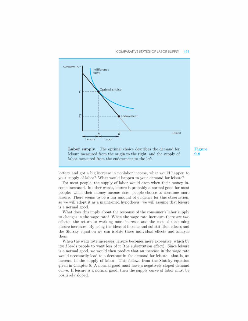
COMPARATIVE STATICS OF LABOR SUPPLY 175
CONSUMPTIONIndifferencecurve
Optimal choiceC
C Endowment
RR LEISURE
Leisure Labor
Labor supply. The optimal choice describes the demand forleisure measured from the origin to the right, and the supply oflabor measured from the endowment to the left.
Figure9.8
lottery and got a big increase in nonlabor income, what would happen toyour supply of labor? What would happen to your demand for leisure?For most people, the supply of labor would drop when their money in-
come increased. In other words, leisure is probably a normal good for mostpeople: when their money income rises, people choose to consume moreleisure. There seems to be a fair amount of evidence for this observation,so we will adopt it as a maintained hypothesis: we will assume that leisureis a normal good.What does this imply about the response of the consumer’s labor supply
to changes in the wage rate? When the wage rate increases there are twoeffects: the return to working more increase and the cost of consumingleisure increases. By using the ideas of income and substitution effects andthe Slutsky equation we can isolate these individual effects and analyzethem.When the wage rate increases, leisure becomes more expensive, which by
itself leads people to want less of it (the substitution effect). Since leisureis a normal good, we would then predict that an increase in the wage ratewould necessarily lead to a decrease in the demand for leisure—that is, anincrease in the supply of labor. This follows from the Slutsky equationgiven in Chapter 8. A normal good must have a negatively sloped demandcurve. If leisure is a normal good, then the supply curve of labor must bepositively sloped.
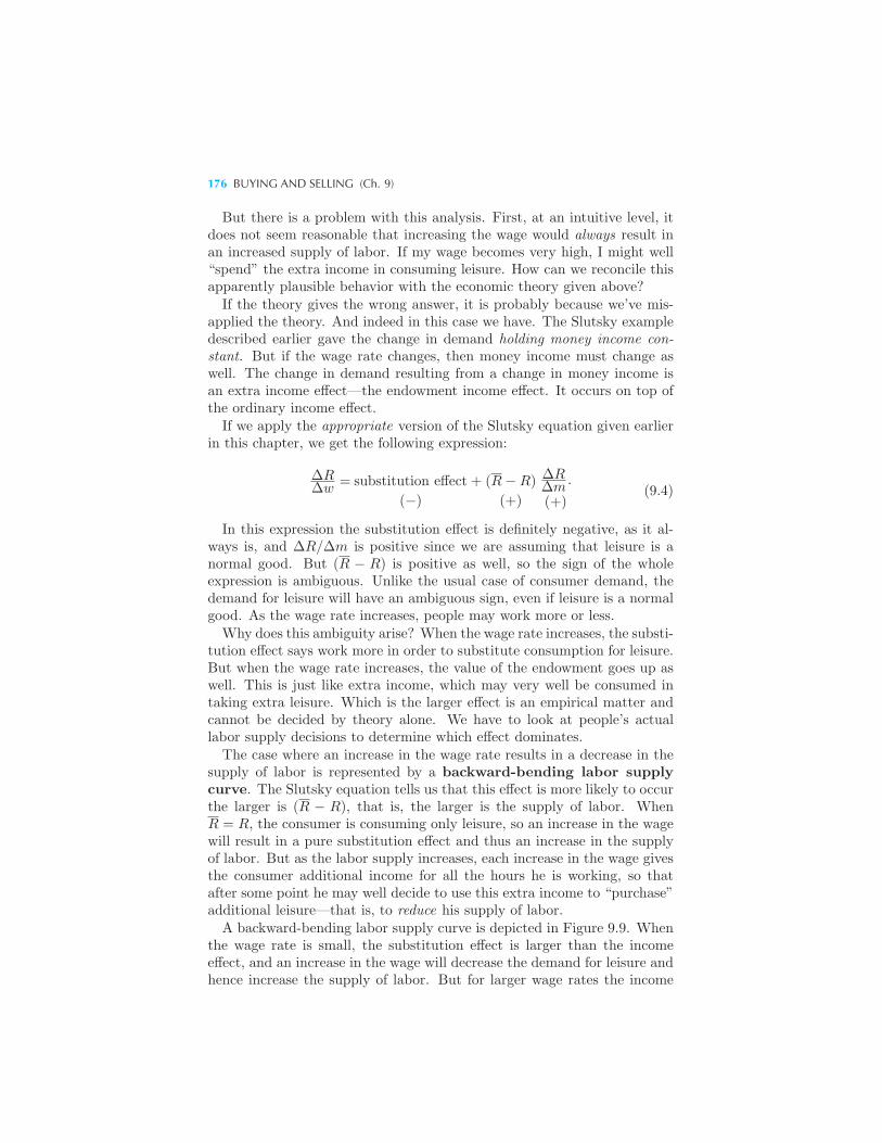
176 BUYING AND SELLING (Ch. 9)
But there is a problem with this analysis. First, at an intuitive level, itdoes not seem reasonable that increasing the wage would always result inan increased supply of labor. If my wage becomes very high, I might well“spend” the extra income in consuming leisure. How can we reconcile thisapparently plausible behavior with the economic theory given above?If the theory gives the wrong answer, it is probably because we’ve mis-
applied the theory. And indeed in this case we have. The Slutsky exampledescribed earlier gave the change in demand holding money income con-stant. But if the wage rate changes, then money income must change aswell. The change in demand resulting from a change in money income isan extra income effect—the endowment income effect. It occurs on top ofthe ordinary income effect.If we apply the appropriate version of the Slutsky equation given earlier
in this chapter, we get the following expression:
ΔRΔw = substitution effect
(−)
+ (R−R)
(+)
ΔRΔm.
(+)(9.4)
In this expression the substitution effect is definitely negative, as it al-ways is, and ΔR/Δm is positive since we are assuming that leisure is anormal good. But (R − R) is positive as well, so the sign of the wholeexpression is ambiguous. Unlike the usual case of consumer demand, thedemand for leisure will have an ambiguous sign, even if leisure is a normalgood. As the wage rate increases, people may work more or less.Why does this ambiguity arise? When the wage rate increases, the substi-
tution effect says work more in order to substitute consumption for leisure.But when the wage rate increases, the value of the endowment goes up aswell. This is just like extra income, which may very well be consumed intaking extra leisure. Which is the larger effect is an empirical matter andcannot be decided by theory alone. We have to look at people’s actuallabor supply decisions to determine which effect dominates.The case where an increase in the wage rate results in a decrease in the
supply of labor is represented by a backward-bending labor supplycurve. The Slutsky equation tells us that this effect is more likely to occurthe larger is (R − R), that is, the larger is the supply of labor. WhenR = R, the consumer is consuming only leisure, so an increase in the wagewill result in a pure substitution effect and thus an increase in the supplyof labor. But as the labor supply increases, each increase in the wage givesthe consumer additional income for all the hours he is working, so thatafter some point he may well decide to use this extra income to “purchase”additional leisure—that is, to reduce his supply of labor.A backward-bending labor supply curve is depicted in Figure 9.9. When
the wage rate is small, the substitution effect is larger than the incomeeffect, and an increase in the wage will decrease the demand for leisure andhence increase the supply of labor. But for larger wage rates the income
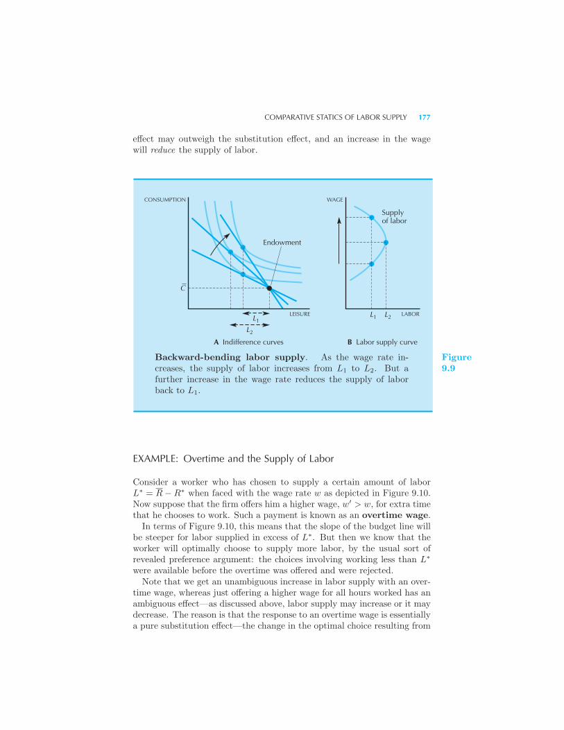
COMPARATIVE STATICS OF LABOR SUPPLY 177
effect may outweigh the substitution effect, and an increase in the wagewill reduce the supply of labor.
CONSUMPTION WAGE
LEISURE LABOR
Supplyof labor
Endowment
C
L
L1
2
A Indifference curves B Labor supply curve
2L1L
Backward-bending labor supply. As the wage rate in-creases, the supply of labor increases from L1 to L2. But afurther increase in the wage rate reduces the supply of laborback to L1.
Figure9.9
EXAMPLE: Overtime and the Supply of Labor
Consider a worker who has chosen to supply a certain amount of laborL∗ = R−R∗ when faced with the wage rate w as depicted in Figure 9.10.Now suppose that the firm offers him a higher wage, w′ > w, for extra timethat he chooses to work. Such a payment is known as an overtime wage.
In terms of Figure 9.10, this means that the slope of the budget line willbe steeper for labor supplied in excess of L∗. But then we know that theworker will optimally choose to supply more labor, by the usual sort ofrevealed preference argument: the choices involving working less than L∗
were available before the overtime was offered and were rejected.Note that we get an unambiguous increase in labor supply with an over-
time wage, whereas just offering a higher wage for all hours worked has anambiguous effect—as discussed above, labor supply may increase or it maydecrease. The reason is that the response to an overtime wage is essentiallya pure substitution effect—the change in the optimal choice resulting from
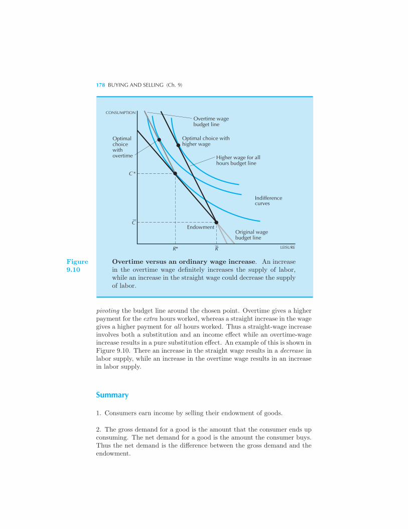
178 BUYING AND SELLING (Ch. 9)
Indifferencecurves
Original wagebudget line
Endowment
Higher wage for allhours budget line
Overtime wagebudget line
Optimal choice withhigher wage
Optimalchoicewithovertime
CONSUMPTION
C *
C
RR* LEISURE
Figure9.10
Overtime versus an ordinary wage increase. An increasein the overtime wage definitely increases the supply of labor,while an increase in the straight wage could decrease the supplyof labor.
pivoting the budget line around the chosen point. Overtime gives a higherpayment for the extra hours worked, whereas a straight increase in the wagegives a higher payment for all hours worked. Thus a straight-wage increaseinvolves both a substitution and an income effect while an overtime-wageincrease results in a pure substitution effect. An example of this is shown inFigure 9.10. There an increase in the straight wage results in a decrease inlabor supply, while an increase in the overtime wage results in an increasein labor supply.
Summary
1. Consumers earn income by selling their endowment of goods.
2. The gross demand for a good is the amount that the consumer ends upconsuming. The net demand for a good is the amount the consumer buys.Thus the net demand is the difference between the gross demand and theendowment.
APPENDIX 179
3. The budget constraint has a slope of −p1/p2 and passes through theendowment bundle.
4. When a price changes, the value of what the consumer has to sell willchange and thereby generate an additional income effect in the Slutskyequation.
5. Labor supply is an interesting example of the interaction of income andsubstitution effects. Due to the interaction of these two effects, the responseof labor supply to a change in the wage rate is ambiguous.
REVIEW QUESTIONS
1. If a consumer’s net demands are (5,−3) and her endowment is (4, 4),what are her gross demands?
2. The prices are (p1, p2) = (2, 3), and the consumer is currently consuming(x1, x2) = (4, 4). There is a perfect market for the two goods in which theycan be bought and sold costlessly. Will the consumer necessarily preferconsuming the bundle (y1, y2) = (3, 5)? Will she necessarily prefer havingthe bundle (y1, y2)?
3. The prices are (p1, p2) = (2, 3), and the consumer is currently consuming(x1, x2) = (4, 4). Now the prices change to (q1, q2) = (2, 4). Could theconsumer be better off under these new prices?
4. The U.S. currently imports about half of the petroleum that it uses. Therest of its needs are met by domestic production. Could the price of oil riseso much that the U.S. would be made better off?
5. Suppose that by some miracle the number of hours in the day increasedfrom 24 to 30 hours (with luck this would happen shortly before examweek). How would this affect the budget constraint?
6. If leisure is an inferior good, what can you say about the slope of thelabor supply curve?
APPENDIX
The derivation of the Slutsky equation in the text contained one bit of handwaving. When we considered how changing the monetary value of the endowmentaffects demand, we said that it was equal to Δxm
1 /Δm. In our old version of theSlutsky equation this was the rate of change in demand when income changedso as to keep the original consumption bundle affordable. But that will not
180 BUYING AND SELLING (Ch. 9)
necessarily be equal to the rate of change of demand when the value of theendowment changes. Let’s examine this point in a little more detail.
Let the price of good 1 change from p1 to p′1, and use m′′ to denote the newmoney income at the price p′1 due to the change in the value of the endowment.Suppose that the price of good 2 remains fixed so we can omit it as an argumentof the demand function.
By definition of m′′, we know that
m′′ −m = Δp1ω1.
Note that it is identically true that
x1(p′1,m
′′)− x1(p1,m)
Δp1=
+x1(p
′1,m
′)− x1(p1,m)
Δp1(substitution effect)
− x1(p′1,m
′)− x1(p′1,m)
Δp1(ordinary income effect)
+x1(p
′1,m
′′)− x1(p′1,m)
Δp1(endowment income effect).
(Just cancel out identical terms with opposite signs on the right-hand side.)By definition of the ordinary income effect,
Δp1 =m′ −m
x1
and by definition of the endowment income effect,
Δp1 =m′′ −m
ω1.
Making these replacements gives us a Slutsky equation of the form
x1(p′1,m
′′)− x1(p1,m)
Δp1=
+x1(p
′1,m
′)− x1(p1,m)
Δp1(substitution effect)
− x1(p′1,m
′)− x1(p′1,m)
m′ −mx1 (ordinary income effect)
+x1(p
′1,m
′′)− x1(p′1,m)
m′′ −mω1 (endowment income effect).
Writing this in terms of Δs, we have
Δx1
Δp1=
Δxs1
Δp1− Δxm
1
Δmx1 +
Δxw1
Δmω1.
APPENDIX 181
The only new term here is the last one. It tells how the demand for good 1changes as income changes, times the endowment of good 1. This is precisely theendowment income effect.
Suppose that we are considering a very small price change, and thus a smallassociated income change. Then the fractions in the two income effects will bevirtually the same, since the rate of change of good 1 when income changes fromm to m′ should be about the same as when income changes from m to m′′. Forsuch small changes we can collect terms and write the last two terms—the incomeeffects—as
Δxm1
Δm(ω1 − x1),
which yields a Slutsky equation of the same form as that derived earlier:
Δx1
Δp1=
Δxs1
Δp1+ (ω1 − x1)
Δxm1
Δm.
If we want to express the Slutsky equation in calculus terms, we can just takelimits in this expression. Or, if you prefer, we can calculate the correct equationdirectly, just by taking partial derivatives. Let x1(p1,m(p1)) be the demandfunction for good 1 where we hold price 2 fixed and recognize that money incomedepends on the price of good 1 via the relationship m(p1) = p1ω1 + p2ω2. Thenwe can write
dx1(p1,m(p1))
dp1=
∂x1(p1,m)
∂p1+
∂x1(p1,m)
∂m
dm(p1)
dp1. (9.5)
By the definition of m(p1) we know how income changes when price changes:
∂m(p1)
∂p1= ω1, (9.6)
and by the Slutsky equation we know how demand changes when price changes,holding money income fixed:
∂x1(p1,m)
∂p1=
∂xs1(p1)
∂p1− ∂x(p1,m)
∂mx1. (9.7)
Inserting equations (9.6) and (9.7) into equation (9.5) we have
dx1(p1,m(p1))
dp1=
∂xs1(p1)
∂p1+
∂x(p1,m)
∂m(ω1 − x1),
which is the form of the Slutsky equation that we want.
CHAPTER 10
INTERTEMPORALCHOICE
In this chapter we continue our examination of consumer behavior by con-sidering the choices involved in saving and consuming over time. Choicesof consumption over time are known as intertemporal choices.
10.1 The Budget Constraint
Let us imagine a consumer who chooses how much of some good to consumein each of two time periods. We will usually want to think of this goodas being a composite good, as described in Chapter 2, but you can thinkof it as being a specific commodity if you wish. We denote the amountof consumption in each period by (c1, c2) and suppose that the prices ofconsumption in each period are constant at 1. The amount of money theconsumer will have in each period is denoted by (m1,m2).
Suppose initially that the only way the consumer has of transferringmoney from period 1 to period 2 is by saving it without earning interest.Furthermore let us assume for the moment that he has no possibility of
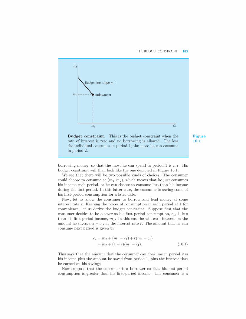
THE BUDGET CONSTRAINT 183
C2
Budget line; slope = –1
Endowmentm2
m1 C1
Budget constraint. This is the budget constraint when therate of interest is zero and no borrowing is allowed. The lessthe individual consumes in period 1, the more he can consumein period 2.
Figure10.1
borrowing money, so that the most he can spend in period 1 is m1. Hisbudget constraint will then look like the one depicted in Figure 10.1.We see that there will be two possible kinds of choices. The consumer
could choose to consume at (m1,m2), which means that he just consumeshis income each period, or he can choose to consume less than his incomeduring the first period. In this latter case, the consumer is saving some ofhis first-period consumption for a later date.Now, let us allow the consumer to borrow and lend money at some
interest rate r. Keeping the prices of consumption in each period at 1 forconvenience, let us derive the budget constraint. Suppose first that theconsumer decides to be a saver so his first period consumption, c1, is lessthan his first-period income, m1. In this case he will earn interest on theamount he saves, m1 − c1, at the interest rate r. The amount that he canconsume next period is given by
c2 = m2 + (m1 − c1) + r(m1 − c1)
= m2 + (1 + r)(m1 − c1). (10.1)
This says that the amount that the consumer can consume in period 2 ishis income plus the amount he saved from period 1, plus the interest thathe earned on his savings.Now suppose that the consumer is a borrower so that his first-period
consumption is greater than his first-period income. The consumer is a
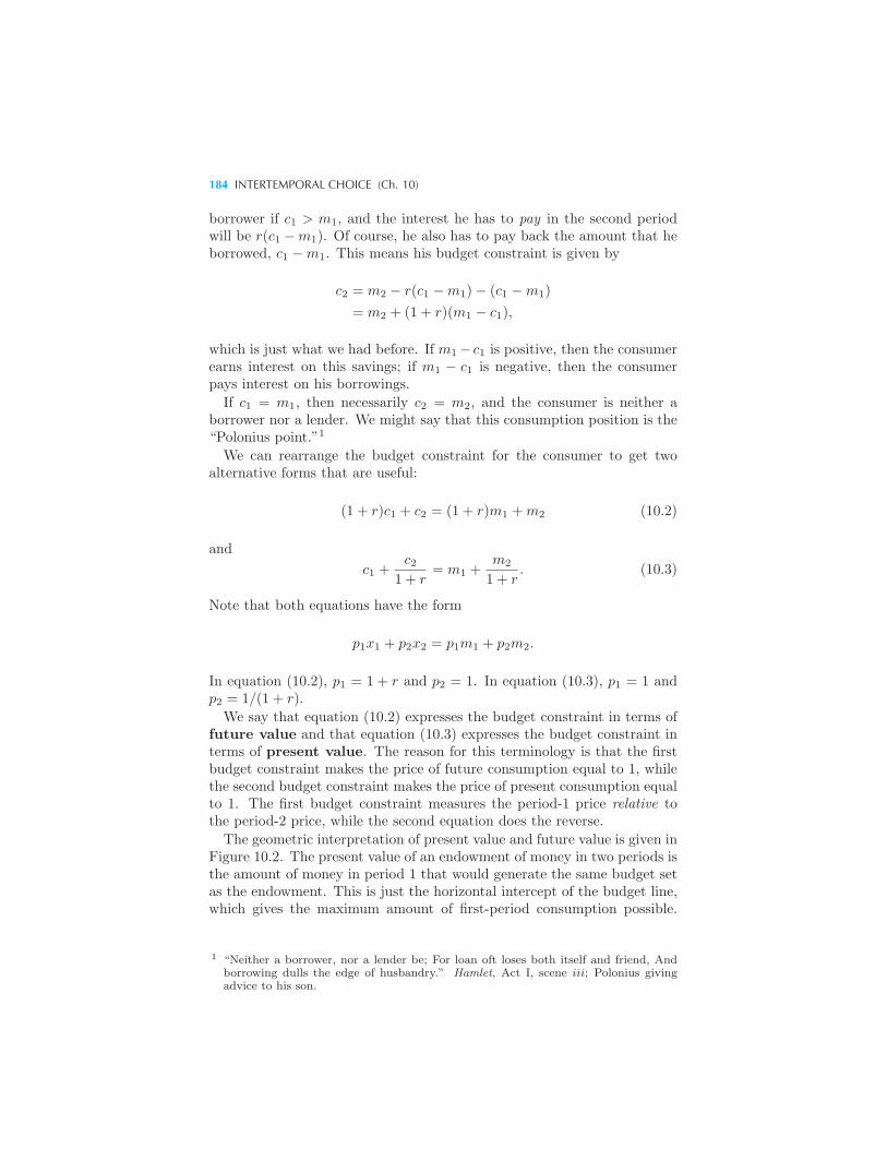
184 INTERTEMPORAL CHOICE (Ch. 10)
borrower if c1 > m1, and the interest he has to pay in the second periodwill be r(c1 −m1). Of course, he also has to pay back the amount that heborrowed, c1 −m1. This means his budget constraint is given by
c2 = m2 − r(c1 −m1)− (c1 −m1)
= m2 + (1 + r)(m1 − c1),
which is just what we had before. If m1− c1 is positive, then the consumerearns interest on this savings; if m1 − c1 is negative, then the consumerpays interest on his borrowings.
If c1 = m1, then necessarily c2 = m2, and the consumer is neither aborrower nor a lender. We might say that this consumption position is the“Polonius point.”1
We can rearrange the budget constraint for the consumer to get twoalternative forms that are useful:
(1 + r)c1 + c2 = (1 + r)m1 +m2 (10.2)
and
c1 +c2
1 + r= m1 +
m2
1 + r. (10.3)
Note that both equations have the form
p1x1 + p2x2 = p1m1 + p2m2.
In equation (10.2), p1 = 1 + r and p2 = 1. In equation (10.3), p1 = 1 andp2 = 1/(1 + r).
We say that equation (10.2) expresses the budget constraint in terms offuture value and that equation (10.3) expresses the budget constraint interms of present value. The reason for this terminology is that the firstbudget constraint makes the price of future consumption equal to 1, whilethe second budget constraint makes the price of present consumption equalto 1. The first budget constraint measures the period-1 price relative tothe period-2 price, while the second equation does the reverse.
The geometric interpretation of present value and future value is given inFigure 10.2. The present value of an endowment of money in two periods isthe amount of money in period 1 that would generate the same budget setas the endowment. This is just the horizontal intercept of the budget line,which gives the maximum amount of first-period consumption possible.
1 “Neither a borrower, nor a lender be; For loan oft loses both itself and friend, Andborrowing dulls the edge of husbandry.” Hamlet, Act I, scene iii; Polonius givingadvice to his son.
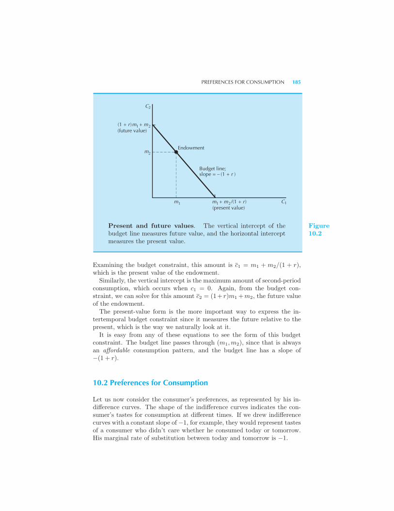
PREFERENCES FOR CONSUMPTION 185
C2
Budget line;slope = – (1 + r )
Endowmentm2
m1 C1m + m1 2/(1 + r )
m + m1 2(1 + r )(future value)
(present value)
Present and future values. The vertical intercept of thebudget line measures future value, and the horizontal interceptmeasures the present value.
Figure10.2
Examining the budget constraint, this amount is c1 = m1 + m2/(1 + r),which is the present value of the endowment.Similarly, the vertical intercept is the maximum amount of second-period
consumption, which occurs when c1 = 0. Again, from the budget con-straint, we can solve for this amount c2 = (1+ r)m1+m2, the future valueof the endowment.The present-value form is the more important way to express the in-
tertemporal budget constraint since it measures the future relative to thepresent, which is the way we naturally look at it.It is easy from any of these equations to see the form of this budget
constraint. The budget line passes through (m1,m2), since that is alwaysan affordable consumption pattern, and the budget line has a slope of−(1 + r).
10.2 Preferences for Consumption
Let us now consider the consumer’s preferences, as represented by his in-difference curves. The shape of the indifference curves indicates the con-sumer’s tastes for consumption at different times. If we drew indifferencecurves with a constant slope of −1, for example, they would represent tastesof a consumer who didn’t care whether he consumed today or tomorrow.His marginal rate of substitution between today and tomorrow is −1.
186 INTERTEMPORAL CHOICE (Ch. 10)
If we drew indifference curves for perfect complements, this would in-dicate that the consumer wanted to consume equal amounts today andtomorrow. Such a consumer would be unwilling to substitute consumptionfrom one time period to the other, no matter what it might be worth tohim to do so.As usual, the intermediate case of well-behaved preferences is the more
reasonable situation. The consumer is willing to substitute some amount ofconsumption today for consumption tomorrow, and how much he is willingto substitute depends on the particular pattern of consumption that hehas.Convexity of preferences is very natural in this context, since it says that
the consumer would rather have an “average” amount of consumption eachperiod rather than have a lot today and nothing tomorrow or vice versa.
10.3 Comparative Statics
Given a consumer’s budget constraint and his preferences for consumptionin each of the two periods, we can examine the optimal choice of consump-tion (c1, c2). If the consumer chooses a point where c1 < m1, we will saythat she is a lender, and if c1 > m1, we say that she is a borrower. InFigure 10.3A we have depicted a case where the consumer is a borrower,and in Figure 10.3B we have depicted a lender.
m c1 1 1
A Borrower B Lender
Indifferencecurve
Choice
Endowment
m
C
c
2
2
2
mc C11 1
Endowment
Indifferencecurve
Choice2c
2m
2C
C
Figure10.3
Borrower and lender. Panel A depicts a borrower, sincec1 > m1, and panel B depicts a lender, since c1 < m1.
Let us now consider how the consumer would react to a change in the
THE SLUTSKY EQUATION AND INTERTEMPORAL CHOICE 187
interest rate. From equation (10.1) we see that increasing the rate of inter-est must tilt the budget line to a steeper position: for a given reduction inc1 you will get more consumption in the second period if the interest rateis higher. Of course the endowment always remains affordable, so the tiltis really a pivot around the endowment.
We can also say something about how the choice of being a borroweror a lender changes as the interest rate changes. There are two cases,depending on whether the consumer is initially a borrower or initially alender. Suppose first that he is a lender. Then it turns out that if theinterest rate increases, the consumer must remain a lender.
This argument is illustrated in Figure 10.4. If the consumer is initially alender, then his consumption bundle is to the left of the endowment point.Now let the interest rate increase. Is it possible that the consumer shiftsto a new consumption point to the right of the endowment?
No, because that would violate the principle of revealed preference:choices to the right of the endowment point were available to the con-sumer when he faced the original budget set and were rejected in favor ofthe chosen point. Since the original optimal bundle is still available at thenew budget line, the new optimal bundle must be a point outside the oldbudget set—which means it must be to the left of the endowment. Theconsumer must remain a lender when the interest rate increases.
There is a similar effect for borrowers: if the consumer is initially aborrower, and the interest rate declines, he or she will remain a borrower.(You might sketch a diagram similar to Figure 10.4 and see if you can spellout the argument.)
Thus if a person is a lender and the interest rate increases, he will remaina lender. If a person is a borrower and the interest rate decreases, he willremain a borrower. On the other hand, if a person is a lender and theinterest rate decreases, he may well decide to switch to being a borrower;similarly, an increase in the interest rate may induce a borrower to becomea lender. Revealed preference tells us nothing about these last two cases.
Revealed preference can also be used to make judgments about how theconsumer’s welfare changes as the interest rate changes. If the consumeris initially a borrower, and the interest rate rises, but he decides to remaina borrower, then he must be worse off at the new interest rate. This argu-ment is illustrated in Figure 10.5; if the consumer remains a borrower, hemust be operating at a point that was affordable under the old budget setbut was rejected, which implies that he must be worse off.
10.4 The Slutsky Equation and Intertemporal Choice
The Slutsky equation can be used to decompose the change in demand dueto an interest rate change into income effects and substitution effects, just
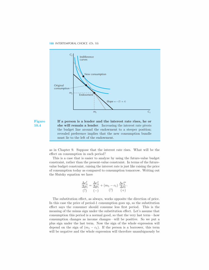
188 INTERTEMPORAL CHOICE (Ch. 10)
CIndifferencecurves
New consumption
Endowment
Originalconsumption
2
2
1 C1m
m
Slope = – (1 + r )
Figure10.4
If a person is a lender and the interest rate rises, he orshe will remain a lender. Increasing the interest rate pivotsthe budget line around the endowment to a steeper position;revealed preference implies that the new consumption bundlemust lie to the left of the endowment.
as in Chapter 9. Suppose that the interest rate rises. What will be theeffect on consumption in each period?This is a case that is easier to analyze by using the future-value budget
constraint, rather than the present-value constraint. In terms of the future-value budget constraint, raising the interest rate is just like raising the priceof consumption today as compared to consumption tomorrow. Writing outthe Slutsky equation we have
Δct1Δp1(?)
=Δcs1Δp1(−)
+ (m1 − c1)
(?)
Δcm1Δm .
(+)
The substitution effect, as always, works opposite the direction of price.In this case the price of period-1 consumption goes up, so the substitutioneffect says the consumer should consume less first period. This is themeaning of the minus sign under the substitution effect. Let’s assume thatconsumption this period is a normal good, so that the very last term—howconsumption changes as income changes—will be positive. So we put aplus sign under the last term. Now the sign of the whole expression willdepend on the sign of (m1 − c1). If the person is a borrower, this termwill be negative and the whole expression will therefore unambiguously be
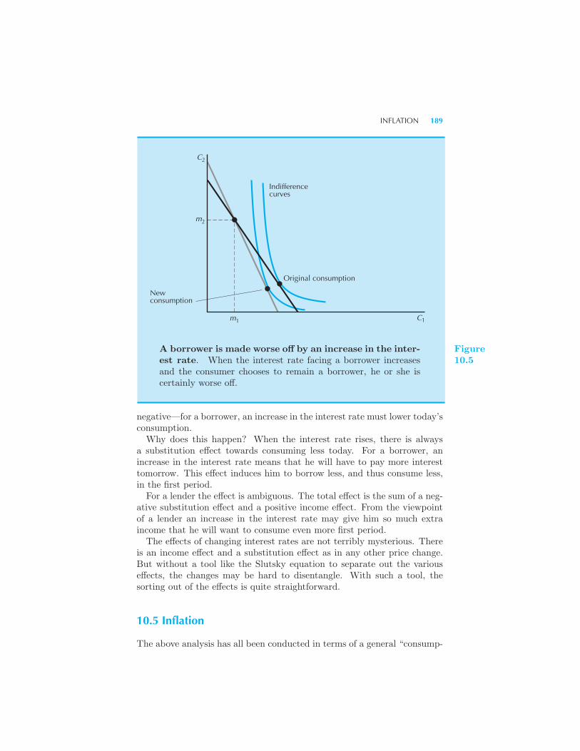
INFLATION 189
m2
2C
1C
Original consumption
Indifference curves
1m
Newconsumption
A borrower is made worse off by an increase in the inter-est rate. When the interest rate facing a borrower increasesand the consumer chooses to remain a borrower, he or she iscertainly worse off.
Figure10.5
negative—for a borrower, an increase in the interest rate must lower today’sconsumption.Why does this happen? When the interest rate rises, there is always
a substitution effect towards consuming less today. For a borrower, anincrease in the interest rate means that he will have to pay more interesttomorrow. This effect induces him to borrow less, and thus consume less,in the first period.For a lender the effect is ambiguous. The total effect is the sum of a neg-
ative substitution effect and a positive income effect. From the viewpointof a lender an increase in the interest rate may give him so much extraincome that he will want to consume even more first period.The effects of changing interest rates are not terribly mysterious. There
is an income effect and a substitution effect as in any other price change.But without a tool like the Slutsky equation to separate out the variouseffects, the changes may be hard to disentangle. With such a tool, thesorting out of the effects is quite straightforward.
10.5 Inflation
The above analysis has all been conducted in terms of a general “consump-
190 INTERTEMPORAL CHOICE (Ch. 10)
tion” good. Giving up Δc units of consumption today buys you (1 + r)Δcunits of consumption tomorrow. Implicit in this analysis is the assumptionthat the “price” of consumption doesn’t change—there is no inflation ordeflation.However, the analysis is not hard to modify to deal with the case of infla-
tion. Let us suppose that the consumption good now has a different pricein each period. It is convenient to choose today’s price of consumption as1 and to let p2 be the price of consumption tomorrow. It is also convenientto think of the endowment as being measured in units of the consumptiongoods as well, so that the monetary value of the endowment in period 2 isp2m2. Then the amount of money the consumer can spend in the secondperiod is given by
p2c2 = p2m2 + (1 + r)(m1 − c1),
and the amount of consumption available second period is
c2 = m2 +1 + r
p2(m1 − c1).
Note that this equation is very similar to the equation given earlier—wejust use (1 + r)/p2 rather than 1 + r.Let us express this budget constraint in terms of the rate of inflation.
The inflation rate, π, is just the rate at which prices grow. Recalling thatp1 = 1, we have
p2 = 1 + π,
which gives us
c2 = m2 +1 + r
1 + π(m1 − c1).
Let’s create a new variable ρ, the real interest rate, and define it by2
1 + ρ =1 + r
1 + π
so that the budget constraint becomes
c2 = m2 + (1 + ρ)(m1 − c1).
One plus the real interest rate measures how much extra consumption youcan get in period 2 if you give up some consumption in period 1. Thatis why it is called the real rate of interest: it tells you how much extraconsumption you can get, not how many extra dollars you can get.
2 The Greek letter ρ, rho, is pronounced “row.”
PRESENT VALUE: A CLOSER LOOK 191
The interest rate on dollars is called the nominal rate of interest. Aswe’ve seen above, the relationship between the two is given by
1 + ρ =1 + r
1 + π.
In order to get an explicit expression for ρ, we write this equation as
ρ =1 + r
1 + π− 1 =
1 + r
1 + π− 1 + π
1 + π
=r − π
1 + π.
This is an exact expression for the real interest rate, but it is common touse an approximation. If the inflation rate isn’t too large, the denominatorof the fraction will be only slightly larger than 1. Thus the real rate ofinterest will be approximately given by
ρ ≈ r − π,
which says that the real rate of interest is just the nominal rate minus therate of inflation. (The symbol ≈ means “approximately equal to.”) Thismakes perfectly good sense: if the interest rate is 18 percent, but pricesare rising at 10 percent, then the real interest rate—the extra consumptionyou can buy next period if you give up some consumption now—will beroughly 8 percent.Of course, we are always looking into the future when making consump-
tion plans. Typically, we know the nominal rate of interest for the nextperiod, but the rate of inflation for next period is unknown. The real inter-est rate is usually taken to be the current interest rate minus the expectedrate of inflation. To the extent that people have different estimates aboutwhat the next year’s rate of inflation will be, they will have different esti-mates of the real interest rate. If inflation can be reasonably well forecast,these differences may not be too large.
10.6 Present Value: A Closer Look
Let us return now to the two forms of the budget constraint describedearlier in section 10.1 in equations (10.2) and (10.3):
(1 + r)c1 + c2 = (1 + r)m1 +m2
andc1 +
c21 + r
= m1 +m2
1 + r.
192 INTERTEMPORAL CHOICE (Ch. 10)
Consider just the right-hand sides of these two equations. We said thatthe first one expresses the value of the endowment in terms of future valueand that the second one expresses it in terms of present value.
Let us examine the concept of future value first. If we can borrow andlend at an interest rate of r, what is the future equivalent of $1 today?The answer is (1 + r) dollars. That is, $1 today can be turned into (1 + r)dollars next period simply by lending it to the bank at an interest rate r.In other words, (1 + r) dollars next period is equivalent to $1 today sincethat is how much you would have to pay next period to purchase—that is,borrow—$1 today. The value (1 + r) is just the price of $1 today, relativeto $1 next period. This can be easily seen from the first budget constraint:it is expressed in terms of future dollars—the second-period dollars have aprice of 1, and first-period dollars are measured relative to them.
What about present value? This is just the reverse: everything is mea-sured in terms of today’s dollars. How much is a dollar next period worthin terms of a dollar today? The answer is 1/(1+r) dollars. This is because1/(1 + r) dollars can be turned into a dollar next period simply by savingit at the rate of interest r. The present value of a dollar to be deliverednext period is 1/(1 + r).
The concept of present value gives us another way to express the budgetfor a two-period consumption problem: a consumption plan is affordable ifthe present value of consumption equals the present value of income.
The idea of present value has an important implication that is closelyrelated to a point made in Chapter 9: if the consumer can freely buy and sellgoods at constant prices, then the consumer would always prefer a higher-valued endowment to a lower-valued one. In the case of intertemporaldecisions, this principle implies that if a consumer can freely borrow andlend at a constant interest rate, then the consumer would always prefer apattern of income with a higher present value to a pattern with a lowerpresent value.
This is true for the same reason that the statement in Chapter 9 wastrue: an endowment with a higher value gives rise to a budget line that isfarther out. The new budget set contains the old budget set, which meansthat the consumer would have all the consumption opportunities she hadwith the old budget set plus some more. Economists sometimes say thatan endowment with a higher present value dominates one with a lowerpresent value in the sense that the consumer can have larger consumptionin every period by selling the endowment with the higher present valuethat she could get by selling the endowment with the lower present value.
Of course, if the present value of one endowment is higher than another,then the future value will be higher as well. However, it turns out that thepresent value is a more convenient way to measure the purchasing powerof an endowment of money over time, and it is the measure to which wewill devote the most attention.
ANALYZING PRESENT VALUE FOR SEVERAL PERIODS 193
10.7 Analyzing Present Value for Several Periods
Let us consider a three-period model. We suppose that we can borrow orlend money at an interest rate r each period and that this interest rate willremain constant over the three periods. Thus the price of consumption inperiod 2 in terms of period-1 consumption will be 1/(1+ r), just as before.
What will the price of period-3 consumption be? Well, if I invest $1today, it will grow into (1+r) dollars next period; and if I leave this moneyinvested, it will grow into (1 + r)2 dollars by the third period. Thus if Istart with 1/(1+ r)2 dollars today, I can turn this into $1 in period 3. Theprice of period-3 consumption relative to period-1 consumption is therefore1/(1 + r)2. Each extra dollar’s worth of consumption in period 3 costs me1/(1 + r)2 dollars today. This implies that the budget constraint will havethe form
c1 +c2
1 + r+
c3(1 + r)2
= m1 +m2
1 + r+
m3
(1 + r)2.
This is just like the budget constraints we’ve seen before, where the priceof period-t consumption in terms of today’s consumption is given by
pt =1
(1 + r)t−1.
As before, moving to an endowment that has a higher present value atthese prices will be preferred by any consumer, since such a change willnecessarily shift the budget set farther out.We have derived this budget constraint under the assumption of constant
interest rates, but it is easy to generalize to the case of changing interestrates. Suppose, for example, that the interest earned on savings from period1 to 2 is r1, while savings from period 2 to 3 earn r2. Then $1 in period 1will grow to (1+ r1)(1+ r2) dollars in period 3. The present value of $1 inperiod 3 is therefore 1/(1 + r1)(1 + r2). This implies that the correct formof the budget constraint is
c1 +c2
1 + r1+
c3(1 + r1)(1 + r2)
= m1 +m2
1 + r1+
m3
(1 + r1)(1 + r2).
This expression is not so hard to deal with, but we will typically be contentto examine the case of constant interest rates.Table 10.1 contains some examples of the present value of $1 T years in
the future at different interest rates. The notable fact about this table ishow quickly the present value goes down for “reasonable” interest rates.For example, at an interest rate of 10 percent, the value of $1 20 years fromnow is only 15 cents.
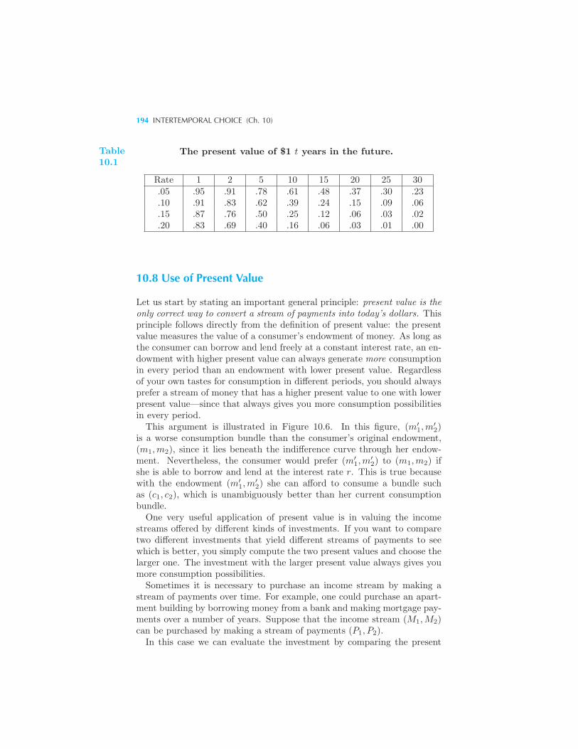
194 INTERTEMPORAL CHOICE (Ch. 10)
Table10.1
The present value of $1 t years in the future.
Rate 1 2 5 10 15 20 25 30.05 .95 .91 .78 .61 .48 .37 .30 .23.10 .91 .83 .62 .39 .24 .15 .09 .06.15 .87 .76 .50 .25 .12 .06 .03 .02.20 .83 .69 .40 .16 .06 .03 .01 .00
10.8 Use of Present Value
Let us start by stating an important general principle: present value is theonly correct way to convert a stream of payments into today’s dollars. Thisprinciple follows directly from the definition of present value: the presentvalue measures the value of a consumer’s endowment of money. As long asthe consumer can borrow and lend freely at a constant interest rate, an en-dowment with higher present value can always generate more consumptionin every period than an endowment with lower present value. Regardlessof your own tastes for consumption in different periods, you should alwaysprefer a stream of money that has a higher present value to one with lowerpresent value—since that always gives you more consumption possibilitiesin every period.This argument is illustrated in Figure 10.6. In this figure, (m′
1,m′2)
is a worse consumption bundle than the consumer’s original endowment,(m1,m2), since it lies beneath the indifference curve through her endow-ment. Nevertheless, the consumer would prefer (m′
1,m′2) to (m1,m2) if
she is able to borrow and lend at the interest rate r. This is true becausewith the endowment (m′
1,m′2) she can afford to consume a bundle such
as (c1, c2), which is unambiguously better than her current consumptionbundle.One very useful application of present value is in valuing the income
streams offered by different kinds of investments. If you want to comparetwo different investments that yield different streams of payments to seewhich is better, you simply compute the two present values and choose thelarger one. The investment with the larger present value always gives youmore consumption possibilities.Sometimes it is necessary to purchase an income stream by making a
stream of payments over time. For example, one could purchase an apart-ment building by borrowing money from a bank and making mortgage pay-ments over a number of years. Suppose that the income stream (M1,M2)can be purchased by making a stream of payments (P1, P2).In this case we can evaluate the investment by comparing the present
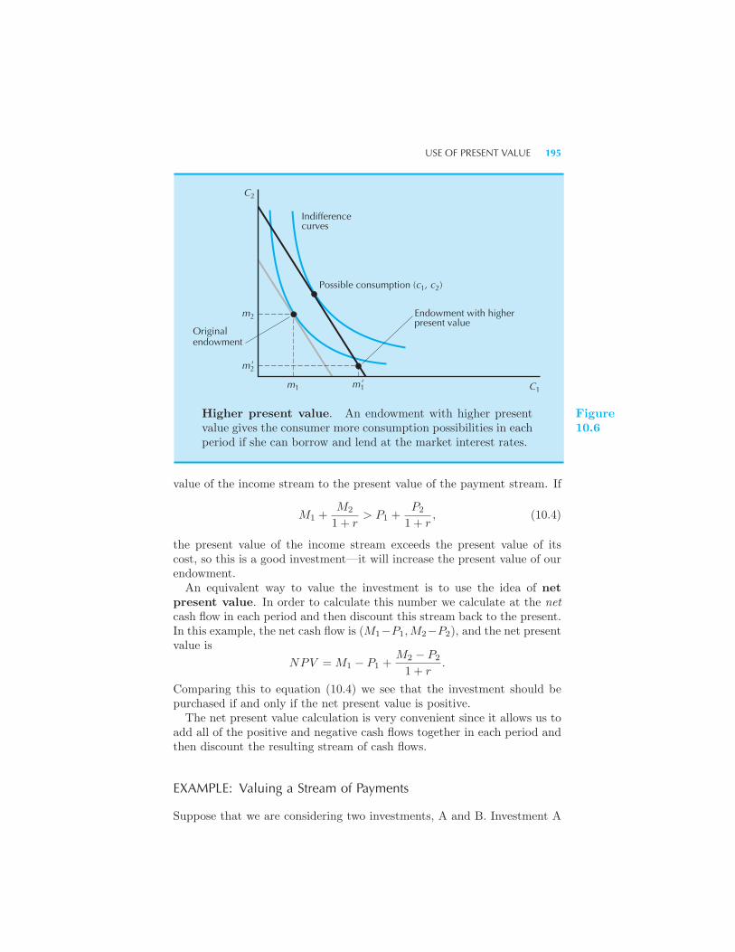
USE OF PRESENT VALUE 195
Indifferencecurves
Possible consumption (c1, c2)
Originalendowment
Endowment with higherpresent value
C1
C2
m2
m1
m2'
m1'
Higher present value. An endowment with higher presentvalue gives the consumer more consumption possibilities in eachperiod if she can borrow and lend at the market interest rates.
Figure10.6
value of the income stream to the present value of the payment stream. If
M1 +M2
1 + r> P1 +
P2
1 + r, (10.4)
the present value of the income stream exceeds the present value of itscost, so this is a good investment—it will increase the present value of ourendowment.An equivalent way to value the investment is to use the idea of net
present value. In order to calculate this number we calculate at the netcash flow in each period and then discount this stream back to the present.In this example, the net cash flow is (M1−P1,M2−P2), and the net presentvalue is
NPV = M1 − P1 +M2 − P2
1 + r.
Comparing this to equation (10.4) we see that the investment should bepurchased if and only if the net present value is positive.The net present value calculation is very convenient since it allows us to
add all of the positive and negative cash flows together in each period andthen discount the resulting stream of cash flows.
EXAMPLE: Valuing a Stream of Payments
Suppose that we are considering two investments, A and B. Investment A
196 INTERTEMPORAL CHOICE (Ch. 10)
pays $100 now and will also pay $200 next year. Investment B pays $0now, and will generate $310 next year. Which is the better investment?The answer depends on the interest rate. If the interest rate is zero, the
answer is clear—just add up the payments. For if the interest rate is zero,then the present-value calculation boils down to summing up the payments.If the interest rate is zero, the present value of investment A is
PVA = 100 + 200 = 300,
and the present value of investment B is
PVB = 0 + 310 = 310,
so B is the preferred investment.But we get the opposite answer if the interest rate is high enough. Sup-
pose, for example, that the interest rate is 20 percent. Then the present-value calculation becomes
PVA = 100 +200
1.20= 266.67
PVB = 0 +310
1.20= 258.33.
Now A is the better investment. The fact that A pays back more moneyearlier means that it will have a higher present value when the interest rateis large enough.
EXAMPLE: The True Cost of a Credit Card
Borrowing money on a credit card is expensive: many companies quoteyearly interest charges of 15 to 21 percent. However, because of the waythese finance charges are computed, the true interest rate on credit carddebt is much higher than this.Suppose that a credit card owner charges a $2000 purchase on the first
day of the month and that the finance charge is 1.5 percent a month. Ifthe consumer pays the entire balance by the end of the month, he does nothave to pay the finance charge. If the consumer pays none of the $2,000,he has to pay a finance charge of $2000 × .015 = $30 at the beginning ofthe next month.What happens if the consumer pays $1,800 towards the $2000 balance
on the last day of the month? In this case, the consumer has borrowedonly $200, so the finance charge should be $3. However, many credit cardcompanies charge the consumers much more than this. The reason is thatmany companies base their charges on the “average monthly balance,” evenif part of that balance is paid by the end of the month. In this example,
USE OF PRESENT VALUE 197
the average monthly balance would be about $2000 (30 days of the $2000balance and 1 day of the $200 balance). The finance charge would thereforebe slightly less than $30, even though the consumer has only borrowed $200.Based on the actual amount of money borrowed, this is an interest rate of15 percent a month!
EXAMPLE: Extending Copyright
Article I, Section 8 of the U.S. Constitution enables Congress to grantpatents and copyrights using this language: “To promote the Progressof Science and useful Arts, by securing for limited Times to Authors andInventors the exclusive Right to their respective Writings and Discoveries.”
But what does “limited Times” mean? The lifetime of a patent in theUnited States is fixed at 20 years; the lifetime for copyright is quite differ-ent.
The first copyright act, passed by Congress in 1790, offered a 14-yearterm along with a 14-year renewal. Subsequently, the copyright term waslengthened to 28 years in 1831, with a 28-year renewal option added in1909. In 1962 the term became 47 years, and 67 years in 1978. In 1967the term was defined as the life of the author plus 50 years, or 75 yearsfor “works for hire.” The 1998 Sonny Bono Copyright Term Extension Actlengthened this term to the life of the author plus 70 years for individualsand 75–95 years for works for hire.
It is questionable whether “the life of the author plus 70 years” shouldbe considered a limited time. One might ask what additional incentive the1998 extension creates for authors to create works?
Let us look at a simple example. Suppose that the interest rate is 7%.Then the increase in present value of extending the copyright term from80 to 100 years is about 0.33% of the present value of the first 80 years.Those extra 20 years have almost no impact on the present value of thecopyright at time of creation since they come so far in the future. Hencethey likely provide miniscule incremental incentive to create the works inthe first place.
Given this tiny increase in value from extending the copyright term whywould it pay anybody to lobby for such a change? The answer is that the1998 act extended the copyright term retroactively so that works that werenear expiration were given a new lease on life.
For example, it has been widely claimed that Disney lobbied heavilyfor the copyright term extension, since the original Mickey Mouse film,Steamboat Willie, was about to go out of copyright.
Retroactive copyright extensions of this sort make no economic sense,since what matters for the authors are the incentives present at the timethe work is created. If there were no such retroactive extension, it is unlikely
198 INTERTEMPORAL CHOICE (Ch. 10)
that anyone would have bothered to ask for copyright extensions given thelow economic value of the additional years of protection.
10.9 Bonds
Securities are financial instruments that promise certain patterns of pay-ment schedules. There are many kinds of financial instruments becausethere are many kinds of payment schedules that people want. Financialmarkets give people the opportunity to trade different patterns of cashflows over time. These cash flows are typically used to finance consump-tion at some time or other.The particular kind of security that we will examine here is a bond.
Bonds are issued by governments and corporations. They are basically away to borrow money. The borrower—the agent who issues the bond—promises to pay a fixed number of dollars x (the coupon) each perioduntil a certain date T (the maturity date), at which point the borrowerwill pay an amount F (the face value) to the holder of the bond.Thus the payment stream of a bond looks like (x, x, x, . . . , F ). If the
interest rate is constant, the present discounted value of such a bond iseasy to compute. It is given by
PV =x
(1 + r)+
x
(1 + r)2+ · · ·+ F
(1 + r)T.
Note that the present value of a bond will decline if the interest rateincreases. Why is this? When the interest rate goes up the price now for$1 delivered in the future goes down. So the future payments of the bondwill be worth less now.There is a large and developed market for bonds. The market value
of outstanding bonds will fluctuate as the interest rate fluctuates sincethe present value of the stream of payments represented by the bond willchange.An interesting special kind of a bond is a bond that makes payments
forever. These are called consols or perpetuities. Suppose that we con-sider a consol that promises to pay x a year forever. To compute the valueof this consol we have to compute the infinite sum:
PV =x
1 + r+
x
(1 + r)2+ · · · .
The trick to computing this is to factor out 1/(1 + r) to get
PV =1
1 + r
[x+
x
(1 + r)+
x
(1 + r)2+ · · ·
].
BONDS 199
But the term in the brackets is just x plus the present value! Substitutingand solving for PV :
PV =1
(1 + r)[x+ PV ]
=x
r.
This wasn’t hard to do, but there is an easy way to get the answer rightoff. How much money, V , would you need at an interest rate r to get xdollars forever? Just write down the equation
V r = x,
which says that the interest on V must equal x. But then the value of suchan investment is given by
V =x
r.
Thus it must be that the present value of a consol that promises to pay xdollars forever must be given by x/r.For a consol it is easy to see directly how increasing the interest rate
reduces the value of a bond. Suppose, for example, that a consol is issuedwhen the interest rate is 10 percent. Then if it promises to pay $10 a yearforever, it will be worth $100 now—since $100 would generate $10 a yearin interest income.Now suppose that the interest rate goes up to 20 percent. The value of
the consol must fall to $50, since it only takes $50 to earn $10 a year at a20 percent interest rate.The formula for the consol can be used to calculate an approximate value
of a long-term bond. If the interest rate is 10 percent, for example, thevalue of $1 30 years from now is only 6 cents. For the size of interest rateswe usually encounter, 30 years might as well be infinity.
EXAMPLE: Installment Loans
Suppose that you borrow $1000 that you promise to pay back in 12 monthlyinstallments of $100 each. What rate of interest are you paying?At first glance it seems that your interest rate is 20 percent: you have
borrowed $1000, and you are paying back $1200. But this analysis is incor-rect. For you haven’t really borrowed $1000 for an entire year. You haveborrowed $1000 for a month, and then you pay back $100. Then you onlyhave borrowed $900, and you owe only a month’s interest on the $900. Youborrow that for a month and then pay back another $100. And so on.The stream of payments that we want to value is
(1000,−100,−100, . . . ,−100).
We can find the interest rate that makes the present value of this streamequal to zero by using a calculator or a computer. The actual interest ratethat you are paying on the installment loan is about 35 percent!
200 INTERTEMPORAL CHOICE (Ch. 10)
10.10 Taxes
In the United States, interest payments are taxed as ordinary income. Thismeans that you pay the same tax on interest income as on labor income.Suppose that your marginal tax bracket is t, so that each extra dollar ofincome, Δm, increases your tax liability by tΔm. Then if you invest Xdollars in an asset, you’ll receive an interest payment of rX. But you’llalso have to pay taxes of trX on this income, which will leave you withonly (1 − t)rX dollars of after-tax income. We call the rate (1 − t)r theafter-tax interest rate.
What if you decide to borrow X dollars, rather than lend them? Thenyou’ll have to make an interest payment of rX. In the United States, someinterest payments are tax deductible and some are not. For example, theinterest payments for a mortgage are tax deductable, but interest paymentson ordinary consumer loans are not. On the other hand, businesses candeduct most kinds of the interest payments that they make.
If a particular interest payment is tax deductible, you can subtract yourinterest payment from your other income and only pay taxes on what’s left.Thus the rX dollars you pay in interest will reduce your tax payments bytrX. The total cost of the X dollars you borrowed will be rX − trX =(1− t)rX.
Thus the after-tax interest rate is the same whether you are borrowingor lending, for people in the same tax bracket. The tax on saving willreduce the amount of money that people want to save, but the subsidy onborrowing will increase the amount of money that people want to borrow.
EXAMPLE: Scholarships and Savings
Many students in the United States receive some form of financial aid tohelp defray college costs. The amount of financial aid a student receivesdepends on many factors, but one important factor is the family’s ability topay for college expenses. Most U.S. colleges and universities use a standardmeasure of ability to pay calculated by the College Entrance ExaminationBoard (CEEB).
If a student wishes to apply for financial aid, his or her family must fillout a questionnaire describing their financial circumstances. The CEEBuses the information on the income and assets of the parents to constructa measure of “adjusted available income.” The fraction of their adjustedavailable income that parents are expected to contribute varies between22 and 47 percent, depending on income. In 1985, parents with a totalbefore-tax income of around $35,000 dollars were expected to contributeabout $7000 toward college expenses.
CHOICE OF THE INTEREST RATE 201
Each additional dollar of assets that the parents accumulate increasestheir expected contribution and decreases the amount of financial aid thattheir child can hope to receive. The formula used by the CEEB effectivelyimposes a tax on parents who save for their children’s college education.Martin Feldstein, President of the National Bureau of Economic Research(NBER) and Professor of Economics at Harvard University, calculated themagnitude of this tax.3
Consider the situation of some parents contemplating saving an addi-tional dollar just as their daughter enters college. At a 6 percent rate ofinterest, the future value of a dollar 4 years from now is $1.26. Since federaland state taxes must be paid on interest income, the dollar yields $1.19 inafter-tax income in 4 years. However, since this additional dollar of savingsincreases the total assets of the parents, the amount of aid received by thedaughter goes down during each of her four college years. The effect of this“education tax” is to reduce the future value of the dollar to only 87 centsafter 4 years. This is equivalent to an income tax of 150 percent!Feldstein also examined the savings behavior of a sample of middle-class
households with pre-college children. He estimates that a household withincome of $40,000 a year and two college-age children saves about 50 per-cent less than they would otherwise due to the combination of federal, state,and “education” taxes that they face.
10.11 Choice of the Interest Rate
In the above discussion, we’ve talked about “the interest rate.” In real lifethere are many interest rates: there are nominal rates, real rates, before-taxrates, after-tax rates, short-term rates, long-term rates, and so on. Whichis the “right” rate to use in doing present-value analysis?The way to answer this question is to think about the fundamentals.
The idea of present discounted value arose because we wanted to be ableto convert money at one point in time to an equivalent amount at anotherpoint in time. “The interest rate” is the return on an investment thatallows us to transfer funds in this way.If we want to apply this analysis when there are a variety of interest
rates available, we need to ask which one has the properties most like thestream of payments we are trying to value. If the stream of paymentsis not taxed, we should use an after-tax interest rate. If the stream ofpayments will continue for 30 years, we should use a long-term interestrate. If the stream of payments is risky, we should use the interest rateon an investment with similar risk characteristics. (We’ll have more to saylater about what this last statement actually means.)
3 Martin Feldstein, “College Scholarship Rules and Private Savings,” American Eco-nomic Review, 85, 3 (June 1995).

202 INTERTEMPORAL CHOICE (Ch. 10)
The interest rate measures the opportunity cost of funds—the valueof alternative uses of your money. So every stream of payments should becompared to your best alternative that has similar characteristics in termsof tax treatment, risk, and liquidity.
Summary
1. The budget constraint for intertemporal consumption can be expressedin terms of present value or future value.
2. The comparative statics results derived earlier for general choice prob-lems can be applied to intertemporal consumption as well.
3. The real rate of interest measures the extra consumption that you canget in the future by giving up some consumption today.
4. A consumer who can borrow and lend at a constant interest rate shouldalways prefer an endowment with a higher present value to one with a lowerpresent value.
REVIEW QUESTIONS
1. How much is $1 million to be delivered 20 years in the future worthtoday if the interest rate is 20 percent?
2. As the interest rate rises, does the intertemporal budget constraint be-come steeper or flatter?
3. Would the assumption that goods are perfect substitutes be valid in astudy of intertemporal food purchases?
4. A consumer, who is initially a lender, remains a lender even after adecline in interest rates. Is this consumer better off or worse off after thechange in interest rates? If the consumer becomes a borrower after thechange is he better off or worse off?
5. What is the present value of $100 one year from now if the interest rateis 10%? What is the present value if the interest rate is 5%?
CHAPTER 11
ASSETMARKETS
Assets are goods that provide a flow of services over time. Assets canprovide a flow of consumption services, like housing services, or can providea flow of money that can be used to purchase consumption. Assets thatprovide a monetary flow are called financial assets.
The bonds that we discussed in the last chapter are examples of financialassets. The flow of services they provide is the flow of interest payments.Other sorts of financial assets such as corporate stock provide differentpatterns of cash flows. In this chapter we will examine the functioning ofasset markets under conditions of complete certainty about the future flowof services provided by the asset.
11.1 Rates of Return
Under this admittedly extreme hypothesis, we have a simple principle re-lating asset rates of return: if there is no uncertainty about the cash flowprovided by assets, then all assets have to have the same rate of return.The reason is obvious: if one asset had a higher rate of return than another,and both assets were otherwise identical, then no one would want to buy
204 ASSET MARKETS (Ch. 11)
the asset with the lower rate of return. So in equilibrium, all assets thatare actually held must pay the same rate of return.Let us consider the process by which these rates of return adjust. Con-
sider an asset A that has current price p0 and is expected to have a price ofp1 tomorrow. Everyone is certain about what today’s price of the asset is,and everyone is certain about what tomorrow’s price will be. We supposefor simplicity that there are no dividends or other cash payments betweenperiods 0 and 1. Suppose furthermore that there is another investment, B,that one can hold between periods 0 and 1 that will pay an interest rate ofr. Now consider two possible investment plans: either invest one dollar inasset A and cash it in next period, or invest one dollar in asset B and earninterest of r dollars over the period.What are the values of these two investment plans at the end of the first
period? We first ask how many units of the asset we must purchase tomake a one dollar investment in it. Letting x be this amount we have theequation
p0x = 1
or
x =1
p0.
It follows that the future value of one dollar’s worth of this asset nextperiod will be
FV = p1x =p1p0
.
On the other hand, if we invest one dollar in asset B, we will have 1 + rdollars next period. If assets A and B are both held in equilibrium, thena dollar invested in either one of them must be worth the same amountsecond period. Thus we have an equilibrium condition:
1 + r =p1p0
.
What happens if this equality is not satisfied? Then there is a sure wayto make money. For example, if
1 + r >p1p0
,
people who own asset A can sell one unit for p0 dollars in the first periodand invest the money in asset B. Next period their investment in asset Bwill be worth p0(1 + r), which is greater than p1 by the above equation.This will guarantee that second period they will have enough money torepurchase asset A, and be back where they started from, but now withextra money.
ADJUSTMENTS FOR DIFFERENCES AMONG ASSETS 205
This kind of operation—buying some of one asset and selling some ofanother to realize a sure return—is known as riskless arbitrage, or ar-bitrage for short. As long as there are people around looking for “surethings” we would expect that well-functioning markets should quickly elim-inate any opportunities for arbitrage. Therefore, another way to state ourequilibrium condition is to say that in equilibrium there should be no oppor-tunities for arbitrage. We’ll refer to this as the no arbitrage condition.But how does arbitrage actually work to eliminate the inequality? In the
example given above, we argued that if 1 + r > p1/p0, then anyone whoheld asset A would want to sell it first period, since they were guaranteedenough money to repurchase it second period. But who would they sell itto? Who would want to buy it? There would be plenty of people willingto supply asset A at p0, but there wouldn’t be anyone foolish enough todemand it at that price.This means that supply would exceed demand and therefore the price
will fall. How far will it fall? Just enough to satisfy the arbitrage condition:until 1 + r = p1/p0.
11.2 Arbitrage and Present Value
We can rewrite the arbitrage condition in a useful way by cross multiplyingto get
p0 =p1
1 + r.
This says that the current price of an asset must be its present value.Essentially we have converted the future-value comparison in the arbitragecondition to a present-value comparison. So if the no arbitrage condition issatisfied, then we are assured that assets must sell for their present values.Any deviation from present-value pricing leaves a sure way to make money.
11.3 Adjustments for Differences among Assets
The no arbitrage rule assumes that the asset services provided by the twoassets are identical, except for the purely monetary difference. If the ser-vices provided by the assets have different characteristics, then we wouldwant to adjust for those differences before we blandly assert that the twoassets must have the same equilibrium rate of return.For example, one asset might be easier to sell than the other. We some-
times express this by saying that one asset is more liquid than another.In this case, we might want to adjust the rate of return to take account ofthe difficulty involved in finding a buyer for the asset. Thus a house thatis worth $100,000 is probably a less liquid asset than $100,000 in Treasurybills.
206 ASSET MARKETS (Ch. 11)
Similarly, one asset might be riskier than another. The rate of returnon one asset may be guaranteed, while the rate of return on another assetmay be highly risky. We’ll examine ways to adjust for risk differences inChapter 13.Here we want to consider two other types of adjustment we might make.
One is adjustment for assets that have some return in consumption value,and the other is for assets that have different tax characteristics.
11.4 Assets with Consumption Returns
Many assets pay off only in money. But there are other assets that payoff in terms of consumption as well. The prime example of this is housing.If you own a house that you live in, then you don’t have to rent livingquarters; thus part of the “return” to owning the house is the fact that youget to live in the house without paying rent. Or, put another way, you getto pay the rent for your house to yourself. This latter way of putting itsounds peculiar, but it contains an important insight.It is true that you don’t make an explicit rental payment to yourself for
the privilege of living in your house, but it turns out to be fruitful to thinkof a homeowner as implicitly making such a payment. The implicit rentalrate on your house is the rate at which you could rent a similar house. Or,equivalently, it is the rate at which you could rent your house to someoneelse on the open market. By choosing to “rent your house to yourself” youare forgoing the opportunity of earning rental payments from someone else,and thus incurring an opportunity cost.Suppose that the implicit rental payment on your house would work
out to T dollars per year. Then part of the return to owning your houseis the fact that it generates for you an implicit income of T dollars peryear—the money that you would otherwise have to pay to live in the samecircumstances as you do now.But that is not the entire return on your house. As real estate agents
never tire of telling us, a house is also an investment. When you buy a houseyou pay a significant amount of money for it, and you might reasonablyexpect to earn a monetary return on this investment as well, through anincrease in the value of your house. This increase in the value of an assetis known as appreciation.Let us use A to represent the expected appreciation in the dollar value
of your house over a year. The total return to owning your house is thesum of the rental return, T , and the investment return, A. If your houseinitially cost P , then the total rate of return on your initial investment inhousing is
h =T +A
P.
This total rate of return is composed of the consumption rate of return,T/P , and the investment rate of return, A/P .
TAXATION OF ASSET RETURNS 207
Let us use r to represent the rate of return on other financial assets.Then the total rate of return on housing should, in equilibrium, be equalto r:
r =T +A
P.
Think about it this way. At the beginning of the year, you can invest Pin a bank and earn rP dollars, or you can invest P dollars in a house andsave T dollars of rent and earn A dollars by the end of the year. The totalreturn from these two investments has to be the same. If T +A < rP youwould be better off investing your money in the bank and paying T dollarsin rent. You would then have rP − T > A dollars at the end of the year.If T + A > rP , then housing would be the better choice. (Of course, thisis ignoring the real estate agent’s commission and other transactions costsassociated with the purchase and sale.)Since the total return should rise at the rate of interest, the financial
rate of return A/P will generally be less than the rate of interest. Thusin general, assets that pay off in consumption will in equilibrium have alower financial rate of return than purely financial assets. This means thatbuying consumption goods such as houses, or paintings, or jewelry solelyas a financial investment is probably not a good idea since the rate ofreturn on these assets will probably be lower than the rate of return onpurely financial assets, because part of the price of the asset reflects theconsumption return that people receive from owning such assets. On theother hand, if you place a sufficiently high value on the consumption returnon such assets, or you can generate rental income from the assets, it maywell make sense to buy them. The total return on such assets may wellmake this a sensible choice.
11.5 Taxation of Asset Returns
The Internal Revenue Service distinguishes two kinds of asset returns forpurposes of taxation. The first kind is the dividend or interest return.These are returns that are paid periodically—each year or each month—over the life of the asset. You pay taxes on interest and dividend income atyour ordinary tax rate, the same rate that you pay on your labor income.The second kind of returns are called capital gains. Capital gains occur
when you sell an asset at a price higher than the price at which you boughtit. Capital gains are taxed only when you actually sell the asset. Underthe current tax law, capital gains are taxed at the same rate as ordinaryincome, but there are some proposals to tax them at a more favorable rate.It is sometimes argued that taxing capital gains at the same rate as
ordinary income is a “neutral” policy. However, this claim can be disputedfor at least two reasons. The first reason is that the capital gains taxes areonly paid when the asset is sold, while taxes on dividends or interest are
208 ASSET MARKETS (Ch. 11)
paid every year. The fact that the capital gains taxes are deferred untiltime of sale makes the effective tax rate on capital gains lower than thetax rate on ordinary income.A second reason that equal taxation of capital gains and ordinary income
is not neutral is that the capital gains tax is based on the increase in thedollar value of an asset. If asset values are increasing just because ofinflation, then a consumer may owe taxes on an asset whose real valuehasn’t changed. For example, suppose that a person buys an asset for $100and 10 years later it is worth $200. Suppose that the general price levelalso doubles in this same ten-year period. Then the person would owetaxes on a $100 capital gain even though the purchasing power of his assethadn’t changed at all. This tends to make the tax on capital gains higherthan that on ordinary income. Which of the two effects dominates is acontroversial question.In addition to the differential taxation of dividends and capital gains
there are many other aspects of the tax law that treat asset returns differ-ently. For example, in the United States, municipal bonds, bonds issuedby cities or states, are not taxed by the Federal government. As we indi-cated earlier, the consumption return from owner-occupied housing is nottaxed. Furthermore, in the United States even part of the capital gainsfrom owner-occupied housing is not taxed.The fact that different assets are taxed differently means that the arbi-
trage rule must adjust for the tax differences in comparing rates of return.Suppose that one asset pays a before-tax interest rate, rb, and another as-set pays a return that is tax exempt, re. Then if both assets are held byindividuals who pay taxes on income at rate t, we must have
(1− t)rb = re.
That is, the after-tax return on each asset must be the same. Otherwise,individuals would not want to hold both assets—it would always pay themto switch exclusively to holding the asset that gave them the higher after-tax return. Of course, this discussion ignores other differences in the assetssuch as liquidity, risk, and so on.
11.6 Market Bubbles
Suppose you are contemplating buying a house that is absolutely certainto be worth $220,000 a year from now and that the current interest rate(reflecting your alternative investment opportunities) is 10%. A fair pricefor the house would be the present value, $200,000.Now suppose that things aren’t quite so certain: many people believe
that the house will be worth $220,000 in a year, but there are no guarantees.We would expect that the house would sell for somewhat less than $200,000due to the additional risk associated with purchase.
APPLICATIONS 209
Suppose the year goes by and the house is worth $240,000, far more thananticipated. The house value went up by 20%, even though the prevailinginterest rate was 10%. It may be that this experience will lead people torevise their view about how much the house will be worth in the future—who knows, maybe it will go up by 20% or even more next year.
If many people hold such beliefs, they can bid up the price of housingnow—which may encourage others to make even more optimistic forecastsabout the housing market. As in our discussion of price adjustment, assetsthat people expect to have a higher return than the rate of interest getpushed up in price. The higher price will tend to reduce current demandbut it also may encourage people to expect an even higher return in thefuture.
The first effect—high prices reducing demand—tends to stablize prices.The second effect—high prices leading to an expectation of even higherprices in the future—tends to destabilize prices.
This is an example of an asset bubble. In a bubble, the price of anasset increases, for one reason or another, and this leads people to expectthe price to go up even more in the future. But if they expect the assetprice to rise significantly in the future, they will try to buy more today,pushing prices up even more rapidly.
Financial markets may be subject to such bubbles, particularly when theparticipants are inexperienced. For example, in 2000–01 we saw a dramaticrun-up in the prices of technology stocks and in 2005–06 we saw a bubblein house prices in much of the United States and many other countries.
All bubbles eventually burst. Prices fall and some people are left holdingassets that are worth much less than they paid for them.
The key to avoiding bubbles is to look at economic fundamentals. In themidst of the housing bubble in the United States, the ratio between theprice of a house and the yearly rental rate on an identical house becamefar larger than historical norms. This gap presumably reflected buyers’expectations of future price increases.
Similarly, the ratio of median house prices to median income reachedhistorical highs. Both of these were warning signs that the high priceswere unsustainable.
“This time it’s different” can be a very hazardous belief to hold, partic-ularly when it comes to financial markets.
11.7 Applications
The fact that all riskless assets must earn the same return is obvious, butvery important. It has surprisingly powerful implications for the function-ing of asset markets.
210 ASSET MARKETS (Ch. 11)
Depletable Resources
Let us study the market equilibrium for a depletable resource like oil. Con-sider a competitive oil market, with many suppliers, and suppose for sim-plicity that there are zero costs to extract oil from the ground. Then howwill the price of oil change over time?It turns out that the price of oil must rise at the rate of interest. To see
this, simply note that oil in the ground is an asset like any other asset. Ifit is worthwhile for a producer to hold it from one period to the next, itmust provide a return to him equivalent to the financial return he couldget elsewhere. If we let pt+1 and pt be the prices at times t+1 and t, thenwe have
pt+1 = (1 + r)pt
as our no arbitrage condition in the oil market.The argument boils down to this simple idea: oil in the ground is like
money in the bank. If money in the bank earns a rate of return of r, thenoil in the ground must earn the same rate of return. If oil in the groundearned a higher return than money in the bank, then no one would take oilout of the ground, preferring to wait till later to extract it, thus pushingthe current price of oil up. If oil in the ground earned a lower return thanmoney in the bank, then the owners of oil wells would try to pump their oilout immediately in order to put the money in the bank, thereby depressingthe current price of oil.This argument tells us how the price of oil changes. But what determines
the price level itself? The price level turns out to be determined by thedemand for oil. Let us consider a very simple model of the demand side ofthe market.Suppose that the demand for oil is constant at D barrels a year and
that there is a total world supply of S barrels. Thus we have a total ofT = S/D years of oil left. When the oil has been depleted we will have touse an alternative technology, say liquefied coal, which can be produced ata constant cost of C dollars per barrel. We suppose that liquefied coal is aperfect substitute for oil in all applications.Now, T years from now, when the oil is just being exhausted, how much
must it sell for? Clearly it must sell for C dollars a barrel, the price ofits perfect substitute, liquefied coal. This means that the price today of abarrel of oil, p0, must grow at the rate of interest r over the next T yearsto be equal to C. This gives us the equation
p0(1 + r)T = C
or
p0 =C
(1 + r)T.
APPLICATIONS 211
This expression gives us the current price of oil as a function of theother variables in the problem. We can now ask interesting comparativestatics questions. For example, what happens if there is an unforeseen newdiscovery of oil? This means that T , the number of years remaining of oil,will increase, and thus (1 + r)T will increase, thereby decreasing p0. Soan increase in the supply of oil will, not surprisingly, decrease its currentprice.What if there is a technological breakthrough that decreases the value
of C? Then the above equation shows that p0 must decrease. The priceof oil has to be equal to the price of its perfect substitute, liquefied coal,when liquefied coal is the only alternative.
When to Cut a Forest
Suppose that the size of a forest—measured in terms of the lumber thatyou can get from it—is some function of time, F (t). Suppose further thatthe price of lumber is constant and that the rate of growth of the tree startshigh and gradually declines. If there is a competitive market for lumber,when should the forest be cut for timber?Answer: when the rate of growth of the forest equals the interest rate.
Before that, the forest is earning a higher rate of return than money in thebank, and after that point it is earning less than money in the bank. Theoptimal time to cut a forest is when its growth rate just equals the interestrate.We can express this more formally by looking at the present value of
cutting the forest at time T . This will be
PV =F (T )
(1 + r)T.
We want to find the choice of T that maximizes the present value—thatis, that makes the value of the forest as large as possible. If we choosea very small value of T , the rate of growth of the forest will exceed theinterest rate, which means that the PV would be increasing so it wouldpay to wait a little longer. On the other hand, if we consider a very largevalue of T , the forest would be growing more slowly than the interest rate,so the PV would be decreasing. The choice of T that maximizes presentvalue occurs when the rate of growth of the forest just equals the interestrate.This argument is illustrated in Figure 11.1. In Figure 11.1A we have
plotted the rate of growth of the forest and the rate of growth of a dollarinvested in a bank. If we want to have the largest amount of money atsome unspecified point in the future, we should always invest our moneyin the asset with the highest return available at each point in time. When
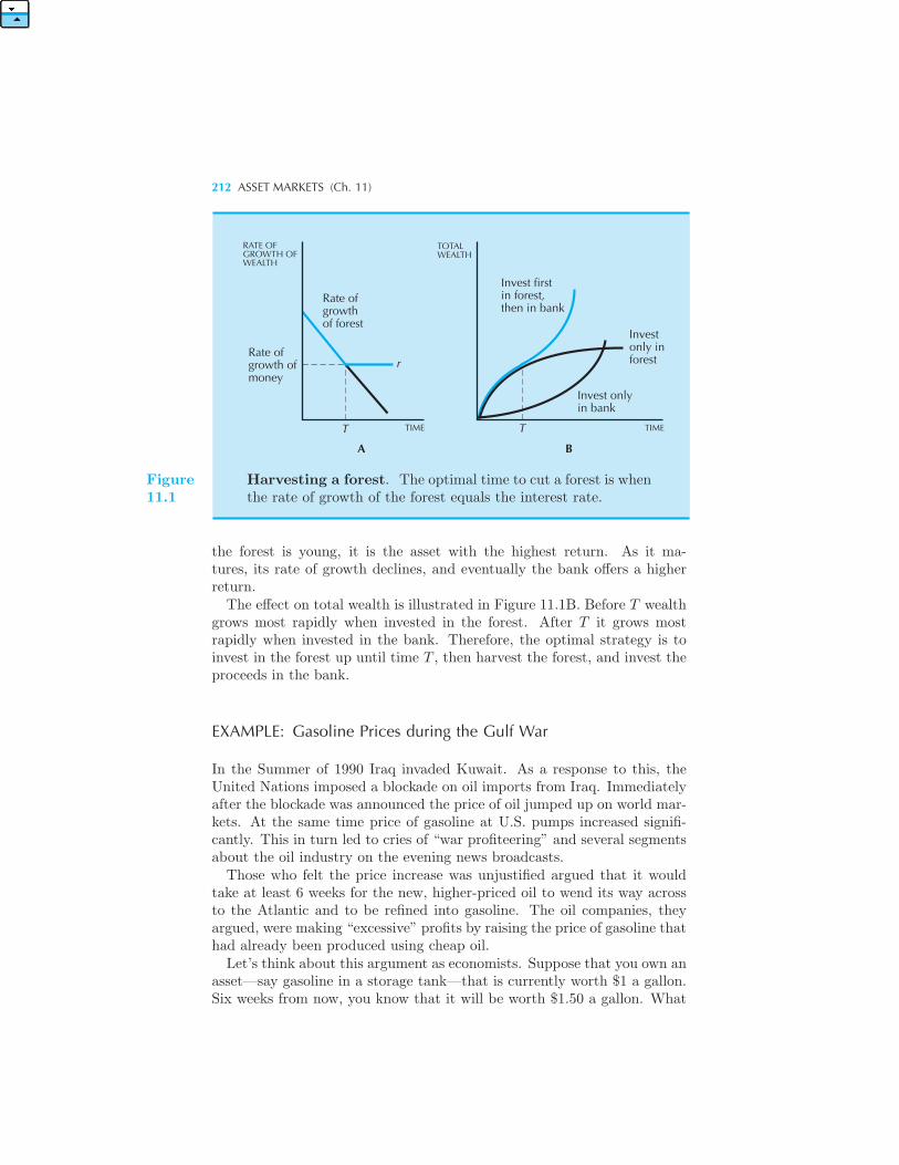
212 ASSET MARKETS (Ch. 11)
TOTALWEALTH
RATE OFGROWTH OF WEALTH
TIME TIME
Rate ofgrowth of forest
Rate ofgrowth ofmoney
Invest firstin forest,then in bank
Invest onlyin bank
Invest only in forest
T T
A B
r
Figure11.1
Harvesting a forest. The optimal time to cut a forest is whenthe rate of growth of the forest equals the interest rate.
the forest is young, it is the asset with the highest return. As it ma-tures, its rate of growth declines, and eventually the bank offers a higherreturn.The effect on total wealth is illustrated in Figure 11.1B. Before T wealth
grows most rapidly when invested in the forest. After T it grows mostrapidly when invested in the bank. Therefore, the optimal strategy is toinvest in the forest up until time T , then harvest the forest, and invest theproceeds in the bank.
EXAMPLE: Gasoline Prices during the Gulf War
In the Summer of 1990 Iraq invaded Kuwait. As a response to this, theUnited Nations imposed a blockade on oil imports from Iraq. Immediatelyafter the blockade was announced the price of oil jumped up on world mar-kets. At the same time price of gasoline at U.S. pumps increased signifi-cantly. This in turn led to cries of “war profiteering” and several segmentsabout the oil industry on the evening news broadcasts.Those who felt the price increase was unjustified argued that it would
take at least 6 weeks for the new, higher-priced oil to wend its way acrossto the Atlantic and to be refined into gasoline. The oil companies, theyargued, were making “excessive” profits by raising the price of gasoline thathad already been produced using cheap oil.Let’s think about this argument as economists. Suppose that you own an
asset—say gasoline in a storage tank—that is currently worth $1 a gallon.Six weeks from now, you know that it will be worth $1.50 a gallon. What
FINANCIAL INSTITUTIONS 213
price will you sell it for now? Certainly you would be foolish to sell itfor much less than $1.50 a gallon—at any price much lower than that youwould be better off letting the gasoline sit in the storage tank for 6 weeks.The same intertemporal arbitrage reasoning about extracting oil from theground applies to gasoline in a storage tank. The (appropriate discounted)price of gasoline tomorrow has to equal the price of gasoline today if youwant firms to supply gasoline today.This makes perfect sense from a welfare point of view as well: if gasoline
is going to be more expensive in the near future, doesn’t it make senseto consume less of it today? The increased price of gasoline encouragesimmediate conservation measures and reflects the true scarcity price ofgasoline.Ironically, the same phenomenon occured two years later in Russia. Dur-
ing the transition to a market economy, Russian oil sold for about $3 abarrel at a time when the world price was about $19 a barrel. The oil pro-ducers anticipated that the price of oil would soon be allowed to rise—sothey tried to hold back as much oil as possible from current production. Asone Russian producer put it, “Have you seen anyone in New York sellingone dollar for 10 cents?” The result was long lines in front of the gasolinepumps for Russian consumers.1
11.8 Financial Institutions
Asset markets allow people to change their pattern of consumption overtime. Consider, for example, two people A and B who have different en-dowments of wealth. A might have $100 today and nothing tomorrow,while B might have $100 tomorrow and nothing today. It might well hap-pen that each would rather have $50 today and $50 tomorrow. But theycan reach this pattern of consumption simply by trading: A gives B $50today, and B gives A $50 tomorrow.In this particular case, the interest rate is zero: A lends B $50 and
only gets $50 in return the next day. If people have convex preferencesover consumption today and tomorrow, they would like to smooth theirconsumption over time, rather than consume everything in one period,even if the interest rate were zero.We can repeat the same kind of story for other patterns of asset endow-
ments. One individual might have an endowment that provides a steadystream of payments and prefer to have a lump sum, while another mighthave a lump sum and prefer a steady stream. For example, a twenty-year-old individual might want to have a lump sum of money now to buy ahouse, while a sixty-year-old might want to have a steady stream of money
1 See Louis Uchitelle, “Russians Line Up for Gas as Refineries Sit on Cheap Oil,” NewYork Times, July 12, 1992, page 4.
214 ASSET MARKETS (Ch. 11)
to finance his retirement. It is clear that both of these individuals couldgain by trading their endowments with each other.In a modern economy financial institutions exist to facilitate these trades.
In the case described above, the sixty-year-old can put his lump sum ofmoney in the bank, and the bank can then lend it to the twenty-year-old.The twenty-year-old then makes mortgage payments to the bank, whichare, in turn, transferred to the sixty-year-old as interest payments. Ofcourse, the bank takes its cut for arranging the trade, but if the bankingindustry is sufficiently competitive, this cut should end up pretty close tothe actual costs of doing business.Banks aren’t the only kind of financial institution that allow one to
reallocate consumption over time. Another important example is the stockmarket. Suppose that an entrepreneur starts a company that becomessuccessful. In order to start the company, the entrepreneur probably hadsome financial backers who put up money to help him get started—to paythe bills until the revenues started rolling in. Once the company has beenestablished, the owners of the company have a claim to the profits thatthe company will generate in the future: they have a claim to a stream ofpayments.But it may well be that they prefer a lump-sum reward for their efforts
now. In this case, the owners can decide to sell the firm to other peoplevia the stock market. They issue shares in the company that entitle theshareholders to a cut of the future profits of the firm in exchange for alump-sum payment now. People who want to purchase part of the streamof profits of the firm pay the original owners for these shares. In this way,both sides of the market can reallocate their wealth over time.There are a variety of other institutions and markets that help facili-
tate intertemporal trade. But what happens when the buyers and sellersaren’t evenly matched? What happens if more people want to sell con-sumption tomorrow than want to buy it? Just as in any market, if thesupply of something exceeds the demand, the price will fall. In this case,the price of consumption tomorrow will fall. We saw earlier that the priceof consumption tomorrow was given by
p =1
1 + r,
so this means that the interest rate must rise. The increase in the interestrate induces people to save more and to demand less consumption now,and thus tends to equate demand and supply.
Summary
1. In equilibrium, all assets with certain payoffs must earn the same rateof return. Otherwise there would be a riskless arbitrage opportunity.
APPENDIX 215
2. The fact that all assets must earn the same return implies that all assetswill sell for their present value.
3. If assets are taxed differently, or have different risk characteristics, thenwe must compare their after-tax rates of return or their risk-adjusted ratesof return.
REVIEW QUESTIONS
1. Suppose asset A can be sold for $11 next period. If assets similar to Aare paying a rate of return of 10%, what must be asset A’s current price?
2. A house, which you could rent for $10,000 a year and sell for $110,000 ayear from now, can be purchased for $100,000. What is the rate of returnon this house?
3. The payments of certain types of bonds (e.g., municipal bonds) are nottaxable. If similar taxable bonds are paying 10% and everyone faces amarginal tax rate of 40%, what rate of return must the nontaxable bondspay?
4. Suppose that a scarce resource, facing a constant demand, will be ex-hausted in 10 years. If an alternative resource will be available at a priceof $40 and if the interest rate is 10%, what must the price of the scarceresource be today?
APPENDIX
Suppose that you invest $1 in an asset yielding an interest rate r where theinterest is paid once a year. Then after T years you will have (1 + r)T dollars.Suppose now that the interest is paid monthly. This means that the monthlyinterest rate will be r/12, and there will be 12T payments, so that after T yearsyou will have (1+r/12)12T dollars. If the interest rate is paid daily, you will have(1 + r/365)365T and so on.
In general, if the interest is paid n times a year, you will have (1 + r/n)nT
dollars after T years. It is natural to ask how much money you will have if theinterest is paid continuously. That is, we ask what is the limit of this expressionas n goes to infinity. It turns out that this is given by the following expression:
erT = limn→∞
(1 + r/n)nT ,
where e is 2.7183 . . ., the base of natural logarithms.This expression for continuous compounding is very convenient for calculations.
For example, let us verify the claim in the text that the optimal time to harvest
216 ASSET MARKETS (Ch. 11)
the forest is when the rate of growth of the forest equals the interest rate. Sincethe forest will be worth F (T ) at time T , the present value of the forest harvestedat time T is
V (T ) =F (T )
erT= e−rTF (T ).
In order to maximize the present value, we differentiate this with respect to Tand set the resulting expression equal to zero. This yields
V ′(T ) = e−rTF ′(T )− re−rTF (T ) = 0
orF ′(T )− rF (T ) = 0.
This can be rearranged to establish the result:
r =F ′(T )
F (T ).
This equation says that the optimal value of T satisfies the condition that therate of interest equals the rate of growth of the value of the forest.

CHAPTER 12
UNCERTAINTY
Uncertainty is a fact of life. People face risks every time they take a shower,walk across the street, or make an investment. But there are financial insti-tutions such as insurance markets and the stock market that can mitigateat least some of these risks. We will study the functioning of these mar-kets in the next chapter, but first we must study individual behavior withrespect to choices involving uncertainty.
12.1 Contingent Consumption
Since we now know all about the standard theory of consumer choice, let’stry to use what we know to understand choice under uncertainty. The firstquestion to ask is what is the basic “thing” that is being chosen?The consumer is presumably concerned with the probability distri-
bution of getting different consumption bundles of goods. A probabilitydistribution consists of a list of different outcomes—in this case, consump-tion bundles—and the probability associated with each outcome. When aconsumer decides how much automobile insurance to buy or how much to
218 UNCERTAINTY (Ch. 12)
invest in the stock market, he is in effect deciding on a pattern of probabilitydistribution across different amounts of consumption.
For example, suppose that you have $100 now and that you are con-templating buying lottery ticket number 13. If number 13 is drawn in thelottery, the holder will be paid $200. This ticket costs, say, $5. The twooutcomes that are of interest are the event that the ticket is drawn and theevent that it isn’t.
Your original endowment of wealth—the amount that you would have ifyou did not purchase the lottery ticket—is $100 if 13 is drawn, and $100if it isn’t drawn. But if you buy the lottery ticket for $5, you will havea wealth distribution consisting of $295 if the ticket is a winner, and $95if it is not a winner. The original endowment of probabilities of wealthin different circumstances has been changed by the purchase of the lotteryticket. Let us examine this point in more detail.
In this discussion we’ll restrict ourselves to examining monetary gamblesfor convenience of exposition. Of course, it is not money alone that mat-ters; it is the consumption that money can buy that is the ultimate “good”being chosen. The same principles apply to gambles over goods, but re-stricting ourselves to monetary outcomes makes things simpler. Second,we will restrict ourselves to very simple situations where there are only afew possible outcomes. Again, this is only for reasons of simplicity.
Above we described the case of gambling in a lottery; here we’ll considerthe case of insurance. Suppose that an individual initially has $35,000worth of assets, but there is a possibility that he may lose $10,000. Forexample, his car may be stolen, or a storm may damage his house. Supposethat the probability of this event happening is p = .01. Then the probabilitydistribution the person is facing is a 1 percent probability of having $25,000of assets, and a 99 percent probability of having $35,000.
Insurance offers a way to change this probability distribution. Supposethat there is an insurance contract that will pay the person $100 if the lossoccurs in exchange for a $1 premium. Of course the premium must be paidwhether or not the loss occurs. If the person decides to purchase $10,000dollars of insurance, it will cost him $100. In this case he will have a 1percent chance of having $34,900 ($35,000 of other assets − $10,000 loss +$10,000 payment from the insurance payment – $100 insurance premium)and a 99 percent chance of having $34,900 ($35,000 of assets − $100 in-surance premium). Thus the consumer ends up with the same wealth nomatter what happens. He is now fully insured against loss.
In general, if this person purchases K dollars of insurance and has to paya premium γK, then he will face the gamble:1
probability .01 of getting $25, 000 +K − γK
1 The Greek letter γ, gamma, is pronounced “gam-ma.”
CONTINGENT CONSUMPTION 219
and
probability .99 of getting $35, 000− γK.
What kind of insurance will this person choose? Well, that depends onhis preferences. He might be very conservative and choose to purchase a lotof insurance, or he might like to take risks and not purchase any insuranceat all. People have different preferences over probability distributions inthe same way that they have different preferences over the consumption ofordinary goods.
In fact, one very fruitful way to look at decision making under uncertaintyis just to think of the money available under different circumstances asdifferent goods. A thousand dollars after a large loss has occurred maymean a very different thing from a thousand dollars when it hasn’t. Ofcourse, we don’t have to apply this idea just to money: an ice cream coneif it happens to be hot and sunny tomorrow is a very different good froman ice cream cone if it is rainy and cold. In general, consumption goods willbe of different value to a person depending upon the circumstances underwhich they become available.
Let us think of the different outcomes of some random event as beingdifferent states of nature. In the insurance example given above therewere two states of nature: the loss occurs or it doesn’t. But in generalthere could be many different states of nature. We can then think ofa contingent consumption plan as being a specification of what willbe consumed in each different state of nature—each different outcome ofthe random process. Contingent means depending on something not yetcertain, so a contingent consumption plan means a plan that depends on theoutcome of some event. In the case of insurance purchases, the contingentconsumption was described by the terms of the insurance contract: howmuch money you would have if a loss occurred and how much you wouldhave if it didn’t. In the case of the rainy and sunny days, the contingentconsumption would just be the plan of what would be consumed given thevarious outcomes of the weather.
People have preferences over different plans of consumption, just likethey have preferences over actual consumption. It certainly might makeyou feel better now to know that you are fully insured. People make choicesthat reflect their preferences over consumption in different circumstances,and we can use the theory of choice that we have developed to analyzethose choices.
If we think about a contingent consumption plan as being just an ordi-nary consumption bundle, we are right back in the framework described inthe previous chapters. We can think of preferences as being defined overdifferent consumption plans, with the “terms of trade” being given by thebudget constraint. We can then model the consumer as choosing the bestconsumption plan he or she can afford, just as we have done all along.
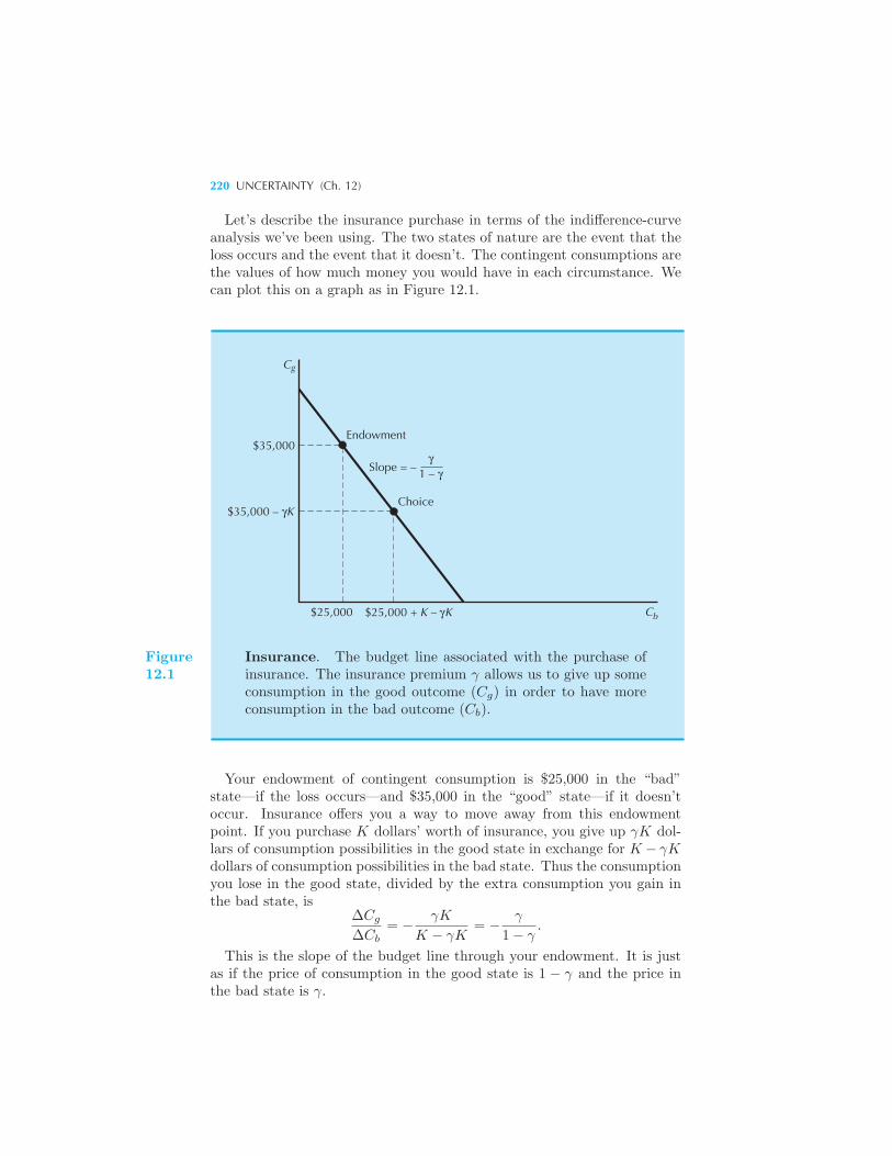
220 UNCERTAINTY (Ch. 12)
Let’s describe the insurance purchase in terms of the indifference-curveanalysis we’ve been using. The two states of nature are the event that theloss occurs and the event that it doesn’t. The contingent consumptions arethe values of how much money you would have in each circumstance. Wecan plot this on a graph as in Figure 12.1.
Cb$25,000 + K – γK
$35,000 – γK
Endowment
Choice
Slope = –γ
1 – γ
Cg
$25,000
$35,000
Figure12.1
Insurance. The budget line associated with the purchase ofinsurance. The insurance premium γ allows us to give up someconsumption in the good outcome (Cg) in order to have moreconsumption in the bad outcome (Cb).
Your endowment of contingent consumption is $25,000 in the “bad”state—if the loss occurs—and $35,000 in the “good” state—if it doesn’toccur. Insurance offers you a way to move away from this endowmentpoint. If you purchase K dollars’ worth of insurance, you give up γK dol-lars of consumption possibilities in the good state in exchange for K − γKdollars of consumption possibilities in the bad state. Thus the consumptionyou lose in the good state, divided by the extra consumption you gain inthe bad state, is
ΔCg
ΔCb= − γK
K − γK= − γ
1− γ.
This is the slope of the budget line through your endowment. It is justas if the price of consumption in the good state is 1 − γ and the price inthe bad state is γ.
CONTINGENT CONSUMPTION 221
We can draw in the indifference curves that a person might have for con-tingent consumption. Here again it is very natural for indifference curvesto have a convex shape: this means that the person would rather have aconstant amount of consumption in each state than a large amount in onestate and a low amount in the other.
Given the indifference curves for consumption in each state of nature,we can look at the choice of how much insurance to purchase. As usual,this will be characterized by a tangency condition: the marginal rate ofsubstitution between consumption in each state of nature should be equalto the price at which you can trade off consumption in those states.
Of course, once we have a model of optimal choice, we can apply all ofthe machinery developed in early chapters to its analysis. We can examinehow the demand for insurance changes as the price of insurance changes,as the wealth of the consumer changes, and so on. The theory of consumerbehavior is perfectly adequate to model behavior under uncertainty as wellas certainty.
EXAMPLE: Catastrophe Bonds
We have seen that insurance is a way to transfer wealth from good statesof nature to bad states of nature. Of course there are two sides to thesetransactions: those who buy insurance and those who sell it. Here we focuson the sell side of insurance.
The sell side of the insurance market is divided into a retail component,which deals directly with end buyers, and a wholesale component, in whichinsurers sell risks to other parties. The wholesale part of the market isknown as the reinsurance market.
Typically, the reinsurance market has relied on large investors such aspension funds to provide financial backing for risks. However, some rein-surers rely on large individual investors. Lloyd’s of London, one of the mostfamous reinsurance consortia, generally uses private investors.
Recently, the reinsurance industry has been experimenting with catas-trophe bonds, which, according to some, are a more flexible way to pro-vide reinsurance. These bonds, generally sold to large institutions, havetypically been tied to natural disasters, like earthquakes or hurricanes.
A financial intermediary, such as a reinsurance company or an invest-ment bank, issues a bond tied to a particular insurable event, such as anearthquake involving, say, at least $500 million in insurance claims. Ifthere is no earthquake, investors are paid a generous interest rate. But ifthe earthquake occurs and the claims exceed the amount specified in thebond, investors sacrifice their principal and interest.
Catastrophe bonds have some attractive features. They can spread riskswidely and can be subdivided indefinitely, allowing each investor to bear
222 UNCERTAINTY (Ch. 12)
only a small part of the risk. The money backing up the insurance is paidin advance, so there is no default risk to the insured.From the economist’s point of view, “cat bonds” are a form of state
contingent security, that is, a security that pays off if and only if someparticular event occurs. This concept was first introduced by Nobel laure-ate Kenneth J. Arrow in a paper published in 1952 and was long thoughtto be of only theoretical interest. But it turned out that all sorts of optionsand other derivatives could be best understood using contingent securi-ties. Now Wall Street rocket scientists draw on this 60-year-old work whencreating exotic new derivatives such as catastrophe bonds.
12.2 Utility Functions and Probabilities
If the consumer has reasonable preferences about consumption in differentcircumstances, then we will be able to use a utility function to describe thesepreferences, just as we have done in other contexts. However, the fact thatwe are considering choice under uncertainty does add a special structureto the choice problem. In general, how a person values consumption in onestate as compared to another will depend on the probability that the statein question will actually occur. In other words, the rate at which I amwilling to substitute consumption if it rains for consumption if it doesn’tshould have something to do with how likely I think it is to rain. Thepreferences for consumption in different states of nature will depend on thebeliefs of the individual about how likely those states are.For this reason, we will write the utility function as depending on the
probabilities as well as on the consumption levels. Suppose that we areconsidering two mutually exclusive states such as rain and shine, loss orno loss, or whatever. Let c1 and c2 represent consumption in states 1 and2, and let π1 and π2 be the probabilities that state 1 or state 2 actuallyoccurs.If the two states are mutually exclusive, so that only one of them can
happen, then π2 = 1− π1. But we’ll generally write out both probabilitiesjust to keep things looking symmetric.Given this notation, we can write the utility function for consumption in
states 1 and 2 as u(c1, c2, π1, π2). This is the function that represents theindividual’s preference over consumption in each state.
EXAMPLE: Some Examples of Utility Functions
We can use nearly any of the examples of utility functions that we’ve seenup until now in the context of choice under uncertainty. One nice exam-ple is the case of perfect substitutes. Here it is natural to weight each
EXPECTED UTILITY 223
consumption by the probability that it will occur. This gives us a utilityfunction of the form
u(c1, c2, π1, π2) = π1c1 + π2c2.
In the context of uncertainty, this kind of expression is known as the ex-pected value. It is just the average level of consumption that you wouldget.Another example of a utility function that might be used to examine
choice under uncertainty is the Cobb–Douglas utility function:
u(c1, c2, π, 1− π) = cπ1 c1−π2 .
Here the utility attached to any combination of consumption bundles de-pends on the pattern of consumption in a nonlinear way.As usual, we can take a monotonic transformation of utility and still
represent the same preferences. It turns out that the logarithm of theCobb-Douglas utility will be very convenient in what follows. This willgive us a utility function of the form
lnu(c1, c2, π1, π2) = π1 ln c1 + π2 ln c2.
12.3 Expected Utility
One particularly convenient form that the utility function might take is thefollowing:
u(c1, c2, π1, π2) = π1v(c1) + π2v(c2).
This says that utility can be written as a weighted sum of some functionof consumption in each state, v(c1) and v(c2), where the weights are givenby the probabilities π1 and π2.
Two examples of this were given above. The perfect substitutes, orexpected value utility function, had this form where v(c) = c. The Cobb-Douglas didn’t have this form originally, but when we expressed it in termsof logs, it had the linear form with v(c) = ln c.
If one of the states is certain, so that π1 = 1, say, then v(c1) is the utilityof certain consumption in state 1. Similarly, if π2 = 1, v(c2) is the utilityof consumption in state 2. Thus the expression
π1v(c1) + π2v(c2)
represents the average utility, or the expected utility, of the pattern ofconsumption (c1, c2).
224 UNCERTAINTY (Ch. 12)
For this reason, we refer to a utility function with the particular formdescribed here as an expected utility function, or, sometimes, a vonNeumann-Morgenstern utility function.2
When we say that a consumer’s preferences can be represented by anexpected utility function, or that the consumer’s preferences have the ex-pected utility property, we mean that we can choose a utility function thathas the additive form described above. Of course we could also choose a dif-ferent form; any monotonic transformation of an expected utility functionis a utility function that describes the same preferences. But the additiveform representation turns out to be especially convenient. If the consumer’spreferences are described by π1 ln c1 + π2 ln c2 they will also be describedby cπ1
1 cπ22 . But the latter representation does not have the expected utility
property, while the former does.On the other hand, the expected utility function can be subjected to
some kinds of monotonic transformation and still have the expected utilityproperty. We say that a function v(u) is a positive affine transfor-mation if it can be written in the form: v(u) = au + b where a > 0. Apositive affine transformation simply means multiplying by a positive num-ber and adding a constant. It turns out that if you subject an expectedutility function to a positive affine transformation, it not only representsthe same preferences (this is obvious since an affine transformation is just aspecial kind of monotonic transformation) but it also still has the expectedutility property.Economists say that an expected utility function is “unique up to an
affine transformation.” This just means that you can apply an affine trans-formation to it and get another expected utility function that representsthe same preferences. But any other kind of transformation will destroythe expected utility property.
12.4 Why Expected Utility Is Reasonable
The expected utility representation is a convenient one, but is it a rea-sonable one? Why would we think that preferences over uncertain choiceswould have the particular structure implied by the expected utility func-tion? As it turns out there are compelling reasons why expected utility isa reasonable objective for choice problems in the face of uncertainty.The fact that outcomes of the random choice are consumption goods
that will be consumed in different circumstances means that ultimatelyonly one of those outcomes is actually going to occur. Either your house
2 John von Neumann was one of the major figures in mathematics in the twentiethcentury. He also contributed several important insights to physics, computer science,and economic theory. Oscar Morgenstern was an economist at Princeton who, alongwith von Neumann, helped to develop mathematical game theory.
WHY EXPECTED UTILITY IS REASONABLE 225
will burn down or it won’t; either it will be a rainy day or a sunny day. Theway we have set up the choice problem means that only one of the manypossible outcomes is going to occur, and hence only one of the contingentconsumption plans will actually be realized.This turns out to have a very interesting implication. Suppose you are
considering purchasing fire insurance on your house for the coming year. Inmaking this choice you will be concerned about wealth in three situations:your wealth now (c0), your wealth if your house burns down (c1), and yourwealth if it doesn’t (c2). (Of course, what you really care about are yourconsumption possibilities in each outcome, but we are simply using wealthas a proxy for consumption here.) If π1 is the probability that your houseburns down and π2 is the probability that it doesn’t, then your preferencesover these three different consumptions can generally be represented by autility function u(π1, π2, c0, c1, c2).
Suppose that we are considering the tradeoff between wealth now andone of the possible outcomes—say, how much money we would be willingto sacrifice now to get a little more money if the house burns down. Thenthis decision should be independent of how much consumption you will havein the other state of nature—how much wealth you will have if the houseis not destroyed. For the house will either burn down or it won’t. If ithappens to burn down, then the value of extra wealth shouldn’t dependon how much wealth you would have if it didn’t burn down. Bygones arebygones—so what doesn’t happen shouldn’t affect the value of consumptionin the outcome that does happen.Note that this is an assumption about an individual’s preferences. It may
be violated. When people are considering a choice between two things, theamount of a third thing they have typically matters. The choice betweencoffee and tea may well depend on how much cream you have. But thisis because you consume coffee together with cream. If you considered achoice where you rolled a die and got either coffee, or tea, or cream, thenthe amount of cream that you might get shouldn’t affect your preferencesbetween coffee and tea. Why? Because you are either getting one thing orthe other: if you end up with cream, the fact that you might have gotteneither coffee or tea is irrelevant.Thus in choice under uncertainty there is a natural kind of “indepen-
dence” between the different outcomes because they must be consumedseparately—in different states of nature. The choices that people plan tomake in one state of nature should be independent from the choices thatthey plan to make in other states of nature. This assumption is known asthe independence assumption. It turns out that this implies that theutility function for contingent consumption will take a very special struc-ture: it has to be additive across the different contingent consumptionbundles.That is, if c1, c2, and c3 are the consumptions in different states of nature,
and π1, π2, and π3 are the probabilities that these three different states of
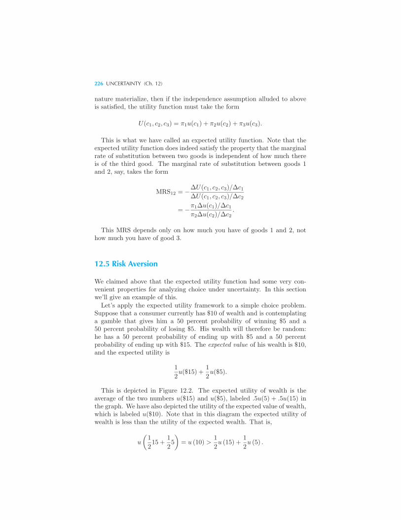
226 UNCERTAINTY (Ch. 12)
nature materialize, then if the independence assumption alluded to aboveis satisfied, the utility function must take the form
U(c1, c2, c3) = π1u(c1) + π2u(c2) + π3u(c3).
This is what we have called an expected utility function. Note that theexpected utility function does indeed satisfy the property that the marginalrate of substitution between two goods is independent of how much thereis of the third good. The marginal rate of substitution between goods 1and 2, say, takes the form
MRS12 = −ΔU(c1, c2, c3)/Δc1ΔU(c1, c2, c3)/Δc2
= −π1Δu(c1)/Δc1π2Δu(c2)/Δc2
.
This MRS depends only on how much you have of goods 1 and 2, nothow much you have of good 3.
12.5 Risk Aversion
We claimed above that the expected utility function had some very con-venient properties for analyzing choice under uncertainty. In this sectionwe’ll give an example of this.Let’s apply the expected utility framework to a simple choice problem.
Suppose that a consumer currently has $10 of wealth and is contemplatinga gamble that gives him a 50 percent probability of winning $5 and a50 percent probability of losing $5. His wealth will therefore be random:he has a 50 percent probability of ending up with $5 and a 50 percentprobability of ending up with $15. The expected value of his wealth is $10,and the expected utility is
1
2u($15) +
1
2u($5).
This is depicted in Figure 12.2. The expected utility of wealth is theaverage of the two numbers u($15) and u($5), labeled .5u(5) + .5u(15) inthe graph. We have also depicted the utility of the expected value of wealth,which is labeled u($10). Note that in this diagram the expected utility ofwealth is less than the utility of the expected wealth. That is,
u
(1
215 +
1
25
)= u (10) >
1
2u (15) +
1
2u (5) .
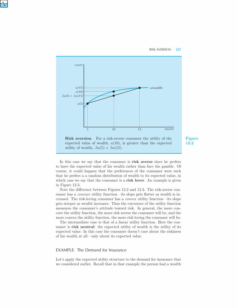
RISK AVERSION 227
UTILITY
u (15)u (10)
.5u (5) + .5u (15)
u (5)
u (wealth)
15105 WEALTH
Risk aversion. For a risk-averse consumer the utility of theexpected value of wealth, u(10), is greater than the expectedutility of wealth, .5u(5) + .5u(15).
Figure12.2
In this case we say that the consumer is risk averse since he prefersto have the expected value of his wealth rather than face the gamble. Ofcourse, it could happen that the preferences of the consumer were suchthat he prefers a a random distribution of wealth to its expected value, inwhich case we say that the consumer is a risk lover. An example is givenin Figure 12.3.Note the difference between Figures 12.2 and 12.3. The risk-averse con-
sumer has a concave utility function—its slope gets flatter as wealth is in-creased. The risk-loving consumer has a convex utility function—its slopegets steeper as wealth increases. Thus the curvature of the utility functionmeasures the consumer’s attitude toward risk. In general, the more con-cave the utility function, the more risk averse the consumer will be, and themore convex the utility function, the more risk loving the consumer will be.The intermediate case is that of a linear utility function. Here the con-
sumer is risk neutral: the expected utility of wealth is the utility of itsexpected value. In this case the consumer doesn’t care about the riskinessof his wealth at all—only about its expected value.
EXAMPLE: The Demand for Insurance
Let’s apply the expected utility structure to the demand for insurance thatwe considered earlier. Recall that in that example the person had a wealth
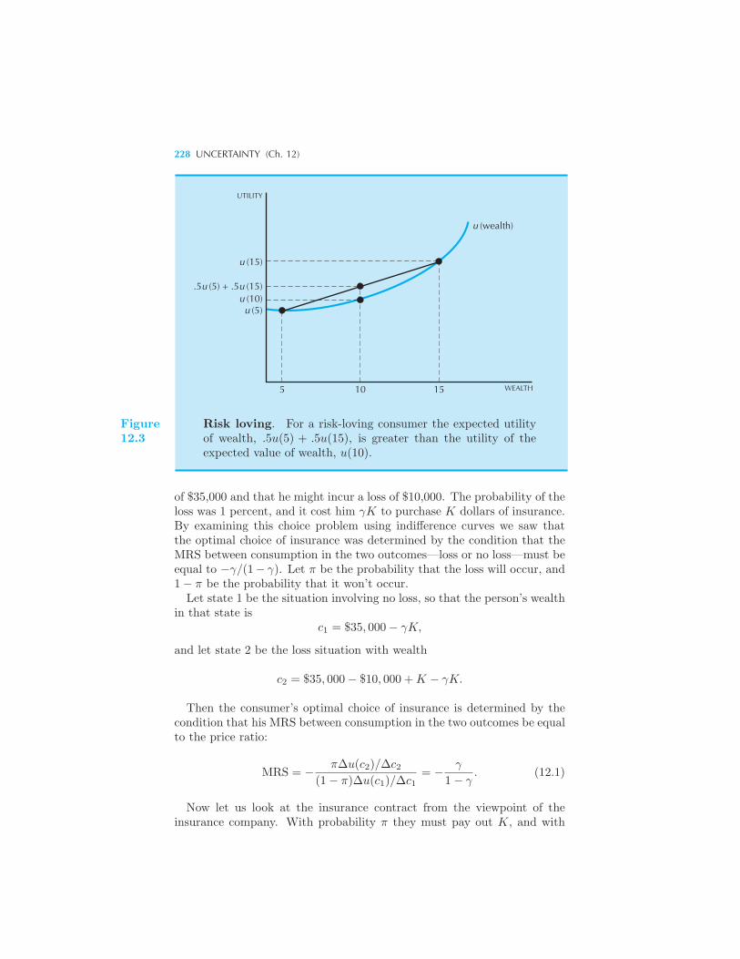
228 UNCERTAINTY (Ch. 12)
u (15)
u (5)u (10)
.5u (5) + .5u (15)
5 10 15 WEALTH
UTILITY
u (wealth)
Figure12.3
Risk loving. For a risk-loving consumer the expected utilityof wealth, .5u(5) + .5u(15), is greater than the utility of theexpected value of wealth, u(10).
of $35,000 and that he might incur a loss of $10,000. The probability of theloss was 1 percent, and it cost him γK to purchase K dollars of insurance.By examining this choice problem using indifference curves we saw thatthe optimal choice of insurance was determined by the condition that theMRS between consumption in the two outcomes—loss or no loss—must beequal to −γ/(1− γ). Let π be the probability that the loss will occur, and1− π be the probability that it won’t occur.Let state 1 be the situation involving no loss, so that the person’s wealth
in that state isc1 = $35, 000− γK,
and let state 2 be the loss situation with wealth
c2 = $35, 000− $10, 000 +K − γK.
Then the consumer’s optimal choice of insurance is determined by thecondition that his MRS between consumption in the two outcomes be equalto the price ratio:
MRS = − πΔu(c2)/Δc2(1− π)Δu(c1)/Δc1
= − γ
1− γ. (12.1)
Now let us look at the insurance contract from the viewpoint of theinsurance company. With probability π they must pay out K, and with
RISK AVERSION 229
probability (1 − π) they pay out nothing. No matter what happens, theycollect the premium γK. Then the expected profit, P , of the insurancecompany is
P = γK − πK − (1− π) · 0 = γK − πK.
Let us suppose that on the average the insurance company just breakseven on the contract. That is, they offer insurance at a “fair” rate, where“fair” means that the expected value of the insurance is just equal to itscost. Then we have
P = γK − πK = 0,
which implies that γ = π.
Inserting this into equation (12.1) we have
πΔu(c2)/Δc2(1− π)Δu(c1)/Δc1
=π
1− π.
Canceling the π’s leaves us with the condition that the optimal amount ofinsurance must satisfy
Δu(c1)
Δc1=
Δu(c2)
Δc2. (12.2)
This equation says that the marginal utility of an extra dollar of income ifthe loss occurs should be equal to the marginal utility of an extra dollar ofincome if the loss doesn’t occur.
Let us suppose that the consumer is risk averse, so that his marginalutility of money is declining as the amount of money he has increases.Then if c1 > c2, the marginal utility at c1 would be less than the marginalutility at c2, and vice versa. Furthermore, if the marginal utilities of incomeare equal at c1 and c2, as they are in equation (12.2), then we must havec1 = c2. Applying the formulas for c1 and c2, we find
35, 000− γK = 25, 000 +K − γK,
which implies that K = $10, 000. This means that when given a chanceto buy insurance at a “fair” premium, a risk-averse consumer will alwayschoose to fully insure.
This happens because the utility of wealth in each state depends only onthe total amount of wealth the consumer has in that state—and not whathe might have in some other state—so that if the total amounts of wealththe consumer has in each state are equal, the marginal utilities of wealthmust be equal as well.
To sum up: if the consumer is a risk-averse, expected utility maximizerand if he is offered fair insurance against a loss, then he will optimallychoose to fully insure.
230 UNCERTAINTY (Ch. 12)
12.6 Diversification
Let us turn now to a different topic involving uncertainty—the benefitsof diversification. Suppose that you are considering investing $100 in twodifferent companies, one that makes sunglasses and one that makes rain-coats. The long-range weather forecasters have told you that next summeris equally likely to be rainy or sunny. How should you invest your money?Wouldn’t it make sense to hedge your bets and put some money in each?
By diversifying your holdings of the two investments, you can get a returnon your investment that is more certain, and therefore more desirable ifyou are a risk-averse person.Suppose, for example, that shares of the raincoat company and the sun-
glasses company currently sell for $10 apiece. If it is a rainy summer, theraincoat company will be worth $20 and the sunglasses company will beworth $5. If it is a sunny summer, the payoffs are reversed: the sunglassescompany will be worth $20 and the raincoat company will be worth $5. Ifyou invest your entire $100 in the sunglasses company, you are taking agamble that has a 50 percent chance of giving you $200 and a 50 percentchance of giving you $50. The same magnitude of payoffs results if youinvest all your money in the sunglasses company: in either case you havean expected payoff of $125.But look what happens if you put half of your money in each. Then,
if it is sunny you get $100 from the sunglasses investment and $25 fromthe raincoat investment. But if it is rainy, you get $100 from the raincoatinvestment and $25 from the sunglasses investment. Either way, you end upwith $125 for sure. By diversifying your investment in the two companies,you have managed to reduce the overall risk of your investment, whilekeeping the expected payoff the same.Diversification was quite easy in this example: the two assets were per-
fectly negatively correlated—when one went up, the other went down. Pairsof assets like this can be extremely valuable because they can reduce riskso dramatically. But, alas, they are also very hard to find. Most assetvalues move together: when GM stock is high, so is Ford stock, and sois Goodrich stock. But as long as asset price movements are not perfectlypositively correlated, there will be some gains from diversification.
12.7 Risk Spreading
Let us return now to the example of insurance. There we considered thesituation of an individual who had $35,000 and faced a .01 probability ofa $10,000 loss. Suppose that there were 1000 such individuals. Then, onaverage, there would be 10 losses incurred, and thus $100,000 lost each year.Each of the 1000 people would face an expected loss of .01 times $10,000, or
ROLE OF THE STOCK MARKET 231
$100 a year. Let us suppose that the probability that any person incurs aloss doesn’t affect the probability that any of the others incur losses. Thatis, let us suppose that the risks are independent.Then each individual will have an expected wealth of .99 × $35, 000 +
.01× $25, 000 = $34, 900. But each individual also bears a large amount ofrisk: each person has a 1 percent probability of losing $10,000.Suppose that each consumer decides to diversify the risk that he or she
faces. How can they do this? Answer: by selling some of their risk toother individuals. Suppose that the 1000 consumers decide to insure oneanother. If anybody incurs the $10,000 loss, each of the 1000 consumerswill contribute $10 to that person. This way, the poor person whose houseburns down is compensated for his loss, and the other consumers have thepeace of mind that they will be compensated if that poor soul happensto be themselves! This is an example of risk spreading: each consumerspreads his risk over all of the other consumers and thereby reduces theamount of risk he bears.Now on the average, 10 houses will burn down a year, so on the average,
each of the 1000 individuals will be paying out $100 a year. But this is juston the average. Some years there might be 12 losses, and other years theremight be 8 losses. The probability is very small that an individual wouldactually have to pay out more than $200, say, in any one year, but even so,the risk is there.But there is even a way to diversify this risk. Suppose that the home-
owners agree to pay $100 a year for certain, whether or not there are anylosses. Then they can build up a cash reserve fund that can be used inthose years when there are multiple fires. They are paying $100 a yearfor certain, and on average that money will be sufficient to compensatehomeowners for fires.As you can see, we now have something very much like a cooperative
insurance company. We could add a few more features: the insurancecompany gets to invest its cash reserve fund and earn interest on its assets,and so on, but the essence of the insurance company is clearly present.
12.8 Role of the Stock Market
The stock market plays a role similar to that of the insurance market inthat it allows for risk spreading. Recall from Chapter 11 that we arguedthat the stock market allowed the original owners of firms to convert theirstream of returns over time to a lump sum. Well, the stock market alsoallows them to convert their risky position of having all their wealth tiedup in one enterprise to a situation where they have a lump sum that theycan invest in a variety of assets. The original owners of the firm have anincentive to issue shares in their company so that they can spread the riskof that single company over a large number of shareholders.
232 UNCERTAINTY (Ch. 12)
Similarly, the later shareholders of a company can use the stock marketto reallocate their risks. If a company you hold shares in is adopting apolicy that is too risky for your taste—or too conservative—you can sellthose shares and purchase others.In the case of insurance, an individual was able to reduce his risk to
zero by purchasing insurance. For a flat fee of $100, the individual couldpurchase full insurance against the $10,000 loss. This was true becausethere was basically no risk in the aggregate: if the probability of the lossoccurring was 1 percent, then on average 10 of the 1000 people would facea loss—we just didn’t know which ones.In the case of the stock market, there is risk in the aggregate. One year
the stock market as a whole might do well, and another year it might dopoorly. Somebody has to bear that kind of risk. The stock market offers away to transfer risky investments from people who don’t want to bear riskto people who are willing to bear risk.Of course, few people outside of Las Vegas like to bear risk: most people
are risk averse. Thus the stock market allows people to transfer risk frompeople who don’t want to bear it to people who are willing to bear it ifthey are sufficiently compensated for it. We’ll explore this idea further inthe next chapter.
Summary
1. Consumption in different states of nature can be viewed as consumptiongoods, and all the analysis of previous chapters can be applied to choiceunder uncertainty.
2. However, the utility function that summarizes choice behavior underuncertainty may have a special structure. In particular, if the utility func-tion is linear in the probabilities, then the utility assigned to a gamble willjust be the expected utility of the various outcomes.
3. The curvature of the expected utility function describes the consumer’sattitudes toward risk. If it is concave, the consumer is a risk averter; andif it is convex, the consumer is a risk lover.
4. Financial institutions such as insurance markets and the stock marketprovide ways for consumers to diversify and spread risks.
REVIEW QUESTIONS
1. How can one reach the consumption points to the left of the endowmentin Figure 12.1?
APPENDIX 233
2. Which of the following utility functions have the expected utility prop-erty? (a) u(c1, c2, π1, π2) = a(π1c1 + π2c2), (b) u(c1, c2, π1, π2) = π1c1 +π2c
22, (c) u(c1, c2, π1, π2) = π1 ln c1 + π2 ln c2 + 17.
3. A risk-averse individual is offered a choice between a gamble that pays$1000 with a probability of 25% and $100 with a probability of 75%, or apayment of $325. Which would he choose?
4. What if the payment was $320?
5. Draw a utility function that exhibits risk-loving behavior for small gam-bles and risk-averse behavior for larger gambles.
6. Why might a neighborhood group have a harder time self insuring forflood damage versus fire damage?
APPENDIX
Let us examine a simple problem to demonstrate the principles of expected utilitymaximization. Suppose that the consumer has some wealth w and is consideringinvesting some amount x in a risky asset. This asset could earn a return of rg inthe “good” outcome, or it could earn a return of rb in the “bad” outcome. Youshould think of rg as being a positive return—the asset increases in value, andrb being a negative return—a decrease in asset value.
Thus the consumer’s wealth in the good and bad outcomes will be
Wg = (w − x) + x(1 + rg) = w + xrg
Wb = (w − x) + x(1 + rb) = w + xrb.
Suppose that the good outcome occurs with probability π and the bad outcomewith probability (1 − π). Then the expected utility if the consumer decides toinvest x dollars is
EU(x) = πu(w + xrg) + (1− π)u(w + xrb).
The consumer wants to choose x so as to maximize this expression.Differentiating with respect to x, we find the way in which utility changes as
x changes:EU ′(x) = πu′(w + xrg)rg + (1− π)u′(w + xrb)rb. (12.3)
The second derivative of utility with respect to x is
EU ′′(x) = πu′′(w + xrg)r2g + (1− π)u′′(w + xrb)r
2b . (12.4)
If the consumer is risk averse his utility function will be concave, which impliesthat u′′(w) < 0 for every level of wealth. Thus the second derivative of expectedutility is unambiguously negative. Expected utility will be a concave functionof x.
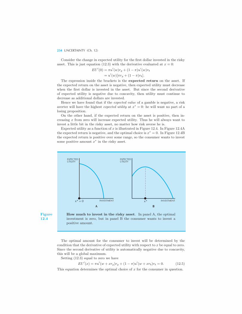
234 UNCERTAINTY (Ch. 12)
Consider the change in expected utility for the first dollar invested in the riskyasset. This is just equation (12.3) with the derivative evaluated at x = 0:
EU ′(0) = πu′(w)rg + (1− π)u′(w)rb
= u′(w)[πrg + (1− π)rb].
The expression inside the brackets is the expected return on the asset. Ifthe expected return on the asset is negative, then expected utility must decreasewhen the first dollar is invested in the asset. But since the second derivativeof expected utility is negative due to concavity, then utility must continue todecrease as additional dollars are invested.
Hence we have found that if the expected value of a gamble is negative, a riskaverter will have the highest expected utility at x∗ = 0: he will want no part of alosing proposition.
On the other hand, if the expected return on the asset is positive, then in-creasing x from zero will increase expected utility. Thus he will always want toinvest a little bit in the risky asset, no matter how risk averse he is.
Expected utility as a function of x is illustrated in Figure 12.4. In Figure 12.4Athe expected return is negative, and the optimal choice is x∗ = 0. In Figure 12.4Bthe expected return is positive over some range, so the consumer wants to investsome positive amount x∗ in the risky asset.
INVESTMENT x*x* = 0
A B
EXPECTEDUTILITY
EXPECTEDUTILITY
INVESTMENT
Figure12.4
How much to invest in the risky asset. In panel A, the optimalinvestment is zero, but in panel B the consumer wants to invest apositive amount.
The optimal amount for the consumer to invest will be determined by thecondition that the derivative of expected utility with respect to x be equal to zero.Since the second derivative of utility is automatically negative due to concavity,this will be a global maximum.
Setting (12.3) equal to zero we have
EU ′(x) = πu′(w + xrg)rg + (1− π)u′(w + xrb)rb = 0. (12.5)
This equation determines the optimal choice of x for the consumer in question.
APPENDIX 235
EXAMPLE: The Effect of Taxation on Investment in Risky Assets
How does the level of investment in a risky asset behave when you tax its return?If the individual pays taxes at rate t, then the after-tax returns will be (1− t)rgand (1− t)rb. Thus the first-order condition determining his optimal investment,x, will be
EU ′(x) = πu′(w + x(1− t)rg)(1− t)rg + (1− π)u′(w + x(1− t)rb)(1− t)rb = 0.
Canceling the (1− t) terms, we have
EU ′(x) = πu′(w + x(1− t)rg)rg + (1− π)u′(w + x(1− t)rb)rb = 0. (12.6)
Let us denote the solution to the maximization problem without taxes—whent = 0—by x∗ and denote the solution to the maximization problem with taxesby x. What is the relationship between x∗ and x?
Your first impulse is probably to think that x∗ > x—that taxation of a riskyasset will tend to discourage investment in it. But that turns out to be exactlywrong! Taxing a risky asset in the way we described will actually encourageinvestment in it!
In fact, there is an exact relation between x∗ and x. It must be the case that
x =x∗
1− t.
The proof is simply to note that this value of x satisfies the first-order conditionfor the optimal choice in the presence of the tax. Substituting this choice intoequation (12.6) we have
EU ′(x) = πu′(w +x∗
1− t(1− t)rg)rg
+ (1− π)u′(w +x∗
1− t(1− t)rb)rb
= πu′(w + x∗rg)rg + (1− π)u′(w + x∗rb)rb = 0,
where the last equality follows from the fact that x∗ is the optimal solution whenthere is no tax.
What is going on here? How can imposing a tax increase the amount ofinvestment in the risky asset? Here is what is happening. When the tax isimposed, the individual will have less of a gain in the good state, but he willalso have less of a loss in the bad state. By scaling his original investment upby 1/(1− t) the consumer can reproduce the same after-tax returns that he hadbefore the tax was put in place. The tax reduces his expected return, but it alsoreduces his risk: by increasing his investment the consumer can get exactly thesame pattern of returns he had before and thus completely offset the effect of thetax. A tax on a risky investment represents a tax on the gain when the return ispositive—but it represents a subsidy on the loss when the return is negative.

CHAPTER 13
RISKYASSETS
In the last chapter we examined a model of individual behavior underuncertainty and the role of two economic institutions for dealing with un-certainty: insurance markets and stock markets. In this chapter we willfurther explore how stock markets serve to allocate risk. In order to dothis, it is convenient to consider a simplified model of behavior under un-certainty.
13.1 Mean-Variance Utility
In the last chapter we examined the expected utility model of choice underuncertainty. Another approach to choice under uncertainty is to describethe probability distributions that are the objects of choice by a few param-eters and think of the utility function as being defined over those param-eters. The most popular example of this approach is the mean-variancemodel. Instead of thinking that a consumer’s preferences depend on theentire probability distribution of his wealth over every possible outcome,we suppose that his preferences can be well described by considering justa few summary statistics about the probability distribution of his wealth.
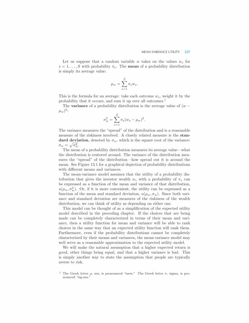
MEAN-VARIANCE UTILITY 237
Let us suppose that a random variable w takes on the values ws fors = 1, . . . , S with probability πs. The mean of a probability distributionis simply its average value:
μw =
S∑s=1
πsws.
This is the formula for an average: take each outcome ws, weight it by theprobability that it occurs, and sum it up over all outcomes.1
The variance of a probability distribution is the average value of (w −μw)
2:
σ2w =
S∑s=1
πs(ws − μw)2.
The variance measures the “spread” of the distribution and is a reasonablemeasure of the riskiness involved. A closely related measure is the stan-dard deviation, denoted by σw, which is the square root of the variance:σw =
√σ2w.
The mean of a probability distribution measures its average value—whatthe distribution is centered around. The variance of the distribution mea-sures the “spread” of the distribution—how spread out it is around themean. See Figure 13.1 for a graphical depiction of probability distributionswith different means and variances.The mean-variance model assumes that the utility of a probability dis-
tribution that gives the investor wealth ws with a probability of πs canbe expressed as a function of the mean and variance of that distribution,u(μw, σ
2w). Or, if it is more convenient, the utility can be expressed as a
function of the mean and standard deviation, u(μw, σw). Since both vari-ance and standard deviation are measures of the riskiness of the wealthdistribution, we can think of utility as depending on either one.This model can be thought of as a simplification of the expected utility
model described in the preceding chapter. If the choices that are beingmade can be completely characterized in terms of their mean and vari-ance, then a utility function for mean and variance will be able to rankchoices in the same way that an expected utility function will rank them.Furthermore, even if the probability distributions cannot be completelycharacterized by their means and variances, the mean-variance model maywell serve as a reasonable approximation to the expected utility model.We will make the natural assumption that a higher expected return is
good, other things being equal, and that a higher variance is bad. Thisis simply another way to state the assumption that people are typicallyaverse to risk.
1 The Greek letter μ, mu, is pronounced “mew.” The Greek letter σ, sigma, is pro-nounced “sig-ma.”
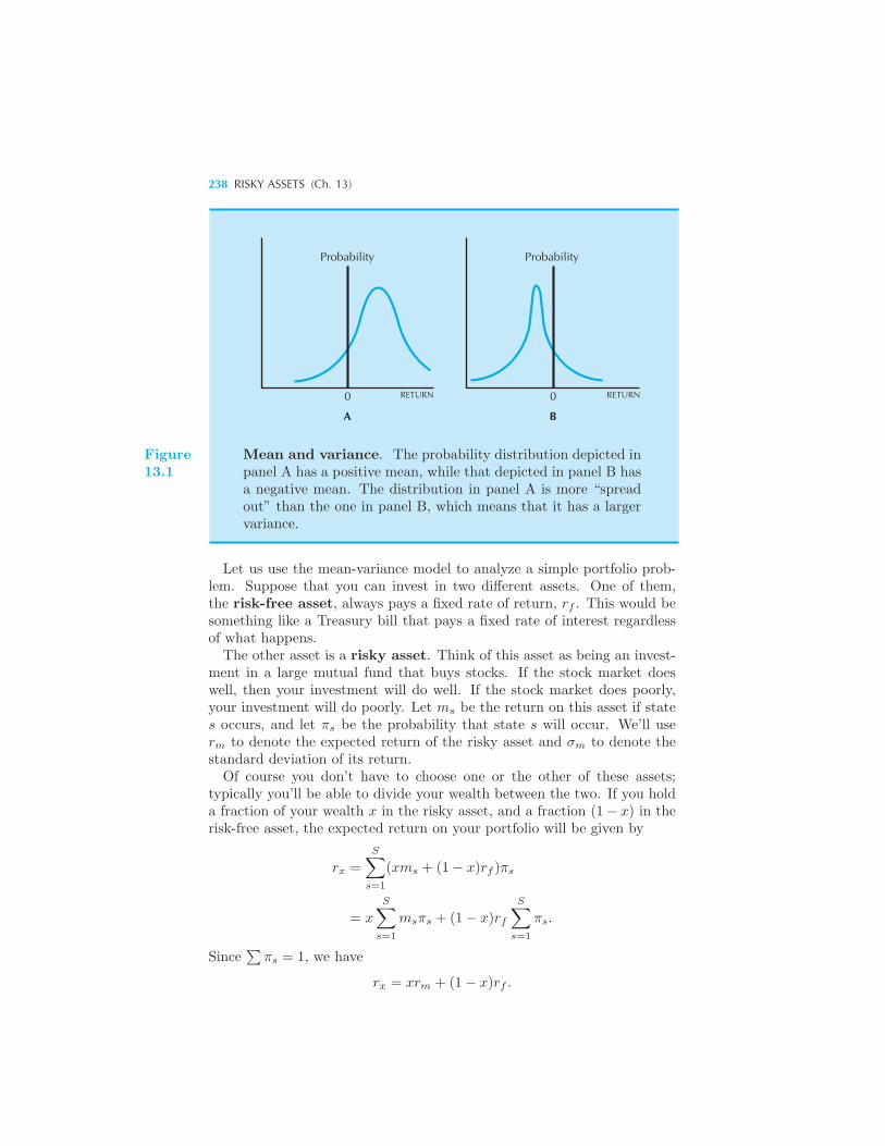
238 RISKY ASSETS (Ch. 13)
Probability Probability
0 0RETURN RETURN
A B
Figure13.1
Mean and variance. The probability distribution depicted inpanel A has a positive mean, while that depicted in panel B hasa negative mean. The distribution in panel A is more “spreadout” than the one in panel B, which means that it has a largervariance.
Let us use the mean-variance model to analyze a simple portfolio prob-lem. Suppose that you can invest in two different assets. One of them,the risk-free asset, always pays a fixed rate of return, rf . This would besomething like a Treasury bill that pays a fixed rate of interest regardlessof what happens.The other asset is a risky asset. Think of this asset as being an invest-
ment in a large mutual fund that buys stocks. If the stock market doeswell, then your investment will do well. If the stock market does poorly,your investment will do poorly. Let ms be the return on this asset if states occurs, and let πs be the probability that state s will occur. We’ll userm to denote the expected return of the risky asset and σm to denote thestandard deviation of its return.Of course you don’t have to choose one or the other of these assets;
typically you’ll be able to divide your wealth between the two. If you holda fraction of your wealth x in the risky asset, and a fraction (1− x) in therisk-free asset, the expected return on your portfolio will be given by
rx =
S∑s=1
(xms + (1− x)rf )πs
= xS∑
s=1
msπs + (1− x)rf
S∑s=1
πs.
Since∑
πs = 1, we have
rx = xrm + (1− x)rf .
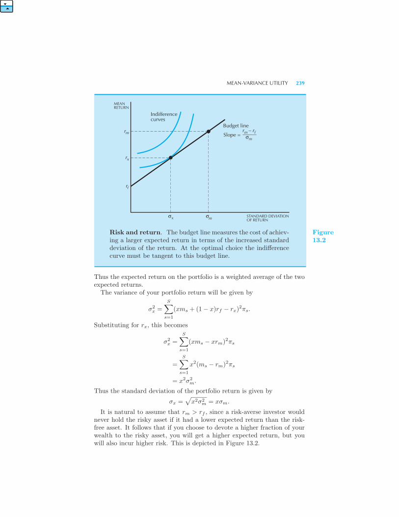
MEAN-VARIANCE UTILITY 239
MEANRETURN
STANDARD DEVIATIONOF RETURN
r
r
r
Indifferencecurves
Budget line
Slope =m
x
f
x mσσ
r – rm
m
fσ
Risk and return. The budget line measures the cost of achiev-ing a larger expected return in terms of the increased standarddeviation of the return. At the optimal choice the indifferencecurve must be tangent to this budget line.
Figure13.2
Thus the expected return on the portfolio is a weighted average of the twoexpected returns.The variance of your portfolio return will be given by
σ2x =
S∑s=1
(xms + (1− x)rf − rx)2πs.
Substituting for rx, this becomes
σ2x =
S∑s=1
(xms − xrm)2πs
=S∑
s=1
x2(ms − rm)2πs
= x2σ2m.
Thus the standard deviation of the portfolio return is given by
σx =√
x2σ2m = xσm.
It is natural to assume that rm > rf , since a risk-averse investor wouldnever hold the risky asset if it had a lower expected return than the risk-free asset. It follows that if you choose to devote a higher fraction of yourwealth to the risky asset, you will get a higher expected return, but youwill also incur higher risk. This is depicted in Figure 13.2.
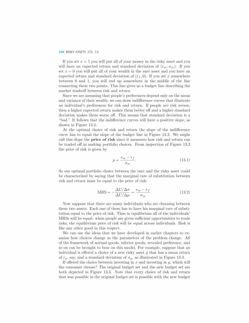
240 RISKY ASSETS (Ch. 13)
If you set x = 1 you will put all of your money in the risky asset and youwill have an expected return and standard deviation of (rm, σm). If youset x = 0 you will put all of your wealth in the sure asset and you have anexpected return and standard deviation of (rf , 0). If you set x somewherebetween 0 and 1, you will end up somewhere in the middle of the lineconnecting these two points. This line gives us a budget line describing themarket tradeoff between risk and return.Since we are assuming that people’s preferences depend only on the mean
and variance of their wealth, we can draw indifference curves that illustratean individual’s preferences for risk and return. If people are risk averse,then a higher expected return makes them better off and a higher standarddeviation makes them worse off. This means that standard deviation is a“bad.” It follows that the indifference curves will have a positive slope, asshown in Figure 13.2.At the optimal choice of risk and return the slope of the indifference
curve has to equal the slope of the budget line in Figure 13.2. We mightcall this slope the price of risk since it measures how risk and return canbe traded off in making portfolio choices. From inspection of Figure 13.2the price of risk is given by
p =rm − rf
σm. (13.1)
So our optimal portfolio choice between the sure and the risky asset couldbe characterized by saying that the marginal rate of substitution betweenrisk and return must be equal to the price of risk:
MRS = −ΔU/Δσ
ΔU/Δμ=
rm − rfσm
. (13.2)
Now suppose that there are many individuals who are choosing betweenthese two assets. Each one of them has to have his marginal rate of substi-tution equal to the price of risk. Thus in equilibrium all of the individuals’MRSs will be equal: when people are given sufficient opportunities to traderisks, the equilibrium price of risk will be equal across individuals. Risk islike any other good in this respect.We can use the ideas that we have developed in earlier chapters to ex-
amine how choices change as the parameters of the problem change. Allof the framework of normal goods, inferior goods, revealed preference, andso on can be brought to bear on this model. For example, suppose that anindividual is offered a choice of a new risky asset y that has a mean returnof ry, say, and a standard deviation of σy, as illustrated in Figure 13.3.
If offered the choice between investing in x and investing in y, which willthe consumer choose? The original budget set and the new budget set areboth depicted in Figure 13.3. Note that every choice of risk and returnthat was possible in the original budget set is possible with the new budget
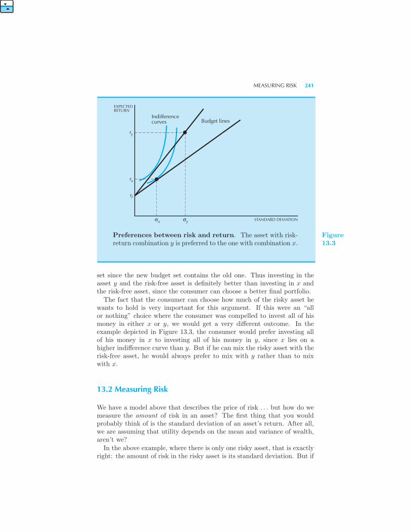
MEASURING RISK 241
σ σ
r
r
r
Budget linesIndifferencecurves
EXPECTEDRETURN
y
x
f
x y STANDARD DEVIATION
Preferences between risk and return. The asset with risk-return combination y is preferred to the one with combination x.
Figure13.3
set since the new budget set contains the old one. Thus investing in theasset y and the risk-free asset is definitely better than investing in x andthe risk-free asset, since the consumer can choose a better final portfolio.
The fact that the consumer can choose how much of the risky asset hewants to hold is very important for this argument. If this were an “allor nothing” choice where the consumer was compelled to invest all of hismoney in either x or y, we would get a very different outcome. In theexample depicted in Figure 13.3, the consumer would prefer investing allof his money in x to investing all of his money in y, since x lies on ahigher indifference curve than y. But if he can mix the risky asset with therisk-free asset, he would always prefer to mix with y rather than to mixwith x.
13.2 Measuring Risk
We have a model above that describes the price of risk . . . but how do wemeasure the amount of risk in an asset? The first thing that you wouldprobably think of is the standard deviation of an asset’s return. After all,we are assuming that utility depends on the mean and variance of wealth,aren’t we?
In the above example, where there is only one risky asset, that is exactlyright: the amount of risk in the risky asset is its standard deviation. But if
242 RISKY ASSETS (Ch. 13)
there are many risky assets, the standard deviation is not an appropriatemeasure for the amount of risk in an asset.This is because a consumer’s utility depends on the mean and variance of
total wealth—not the mean and variance of any single asset that he mighthold. What matters is how the returns of the various assets a consumerholds interact to create a mean and variance of his wealth. As in the restof economics, it is the marginal impact of a given asset on total utilitythat determines its value, not the value of that asset held alone. Just asthe value of an extra cup of coffee may depend on how much cream isavailable, the amount that someone would be willing to pay for an extrashare of a risky asset will depend on how it interacts with other assets inhis portfolio.Suppose, for example, that you are considering purchasing two assets,
and you know that there are only two possible outcomes that can happen.Asset A will be worth either $10 or −$5, and asset B will be worth either−$5 or $10. But when asset A is worth $10, asset B will be worth −$5 andvice versa. In other words the values of the two assets will be negativelycorrelated: when one has a large value, the other will have a small value.Suppose that the two outcomes are equally likely, so that the average
value of each asset will be $2.50. Then if you don’t care about risk at alland you must hold one asset or the other, the most that you would bewilling to pay for either one would be $2.50—the expected value of eachasset. If you are averse to risk, you would be willing to pay even less than$2.50.But what if you can hold both assets? Then if you hold one share of
each asset, you will get $5 whichever outcome arises. Whenever one assetis worth $10, the other is worth −$5. Thus, if you can hold both assets,the amount that you would be willing to pay to purchase both assets wouldbe $5.This example shows in a vivid way that the value of an asset will depend
in general on how it is correlated with other assets. Assets that move inopposite directions—that are negatively correlated with each other—arevery valuable because they reduce overall risk. In general the value of anasset tends to depend much more on the correlation of its return with otherassets than with its own variation. Thus the amount of risk in an assetdepends on its correlation with other assets.It is convenient to measure the risk in an asset relative to the risk in the
stock market as a whole. We call the riskiness of a stock relative to therisk of the market the beta of a stock, and denote it by the Greek letterβ. Thus, if i represents some particular stock, we write βi for its riskinessrelative to the market as a whole. Roughly speaking:
βi =how risky asset i is
how risky the stock market is.
If a stock has a beta of 1, then it is just as risky as the market as a whole;
EQUILIBRIUM IN A MARKET FOR RISKY ASSETS 243
when the market moves up by 10 percent, this stock will, on the average,move up by 10 percent. If a stock has a beta of less than 1, then whenthe market moves up by 10 percent, the stock will move up by less than10 percent. The beta of a stock can be estimated by statistical methodsto determine how sensitive the movements of one variable are relative toanother, and there are many investment advisory services that can provideyou with estimates of the beta of a stock.2
13.3 Counterparty Risk
Financial institutions loan money not just to individuals but to each other.There is always the chance that one party to a loan may fail to repay theloan, a risk known as counterparty risk.To see how this works, imagine 3 banks, A, B, and C. Bank A owes B a
billion dollars, Bank B owes C a billion dollars, and Bank C owes bank A abillion dollars. Now suppose that Bank A runs out of money and defaultson its loan. Bank B is now out a billion dollars and may not be able topay C. Bank C, in turn, can’t pay A, pushing A even further in the hole.This sort of effect is known as financial contagion or systemic risk. Itis a very simplified version of what happened to U.S. financial institutionsin the Fall of 2008.What’s the solution? One way to deal with this sort of problem is to
have a “lender of last resort,” which is typically a central bank, such asthe U.S. Federal Reserve System. Bank A can go to the Federal Reserveand request an emergency loan of a billion dollars. It now pays off its loanfrom Bank B, which in turn pays Bank C, which in turn pays back BankA. Bank A now has sufficient assets to pay back the loan from the centralbank.This is, of course, an overly simplified example. Initially, there was no net
debt among the three banks. If they had gotten together to compare assetsand liabilities, they would have certainly discovered that fact. However,when assets and liabilities span thousands of financial institutions, it maybe difficult to determine net positions, which is why lenders of last resortmay be necessary.
13.4 Equilibrium in a Market for Risky Assets
We are now in a position to state the equilibrium condition for a marketwith risky assets. Recall that in a market with only certain returns, we
2 The Greek letter β, beta, is pronounced “bait-uh.” For those of you who know somestatistics, the beta of a stock is defined to be βi = cov(ri, rm)/var(rm). That is, βi
is the covariance of the return on the stock with the market return divided by thevariance of the market return.
244 RISKY ASSETS (Ch. 13)
saw that all assets had to earn the same rate of return. Here we have asimilar principle: all assets, after adjusting for risk, have to earn the samerate of return.The catch is about adjusting for risk. How do we do that? The answer
comes from the analysis of optimal choice given earlier. Recall that weconsidered the choice of an optimal portfolio that contained a riskless assetand a risky asset. The risky asset was interpreted as being a mutual fund—a diversified portfolio including many risky assets. In this section we’llsuppose that this portfolio consists of all risky assets.
Then we can identify the expected return on this market portfolio ofrisky assets with the market expected return, rm, and identify the standarddeviation of the market return with the market risk, σm. The return onthe safe asset is rf , the risk-free return.We saw in equation (13.1) that the price of risk, p, is given by
p =rm − rf
σm.
We said above that the amount of risk in a given asset i relative to thetotal risk in the market is denoted by βi. This means that to measure thetotal amount of risk in asset i, we have to multiply by the market risk, σm.Thus the total risk in asset i is given by βiσm.What is the cost of this risk? Just multiply the total amount of risk,
βiσm, by the price of risk. This gives us the risk adjustment:
risk adjustment = βiσmp
= βiσmrm − rf
σm
= βi(rm − rf ).
Now we can state the equilibrium condition in markets for risky assets:in equilibrium all assets should have the same risk-adjusted rate of return.The logic is just like the logic used in Chapter 12: if one asset had ahigher risk-adjusted rate of return than another, everyone would want tohold the asset with the higher risk-adjusted rate. Thus in equilibrium therisk-adjusted rates of return must be equalized.If there are two assets i and j that have expected returns ri and rj
and betas of βi and βj , we must have the following equation satisfied inequilibrium:
ri − βi(rm − rf ) = rj − βj(rm − rf ).
This equation says that in equilibrium the risk-adjusted returns on the twoassets must be the same—where the risk adjustment comes from multiply-ing the total risk of the asset by the price of risk.Another way to express this condition is to note the following. The risk-
free asset, by definition, must have βf = 0. This is because it has zero risk,
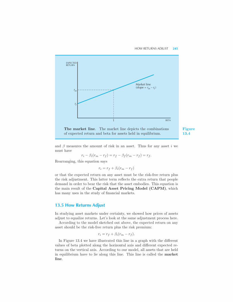
HOW RETURNS ADJUST 245
EXPECTEDRETURN
r
fr
m
BETA1
Market line(slope = r – r )fm
The market line. The market line depicts the combinationsof expected return and beta for assets held in equilibrium.
Figure13.4
and β measures the amount of risk in an asset. Thus for any asset i wemust have
ri − βi(rm − rf ) = rf − βf (rm − rf ) = rf .
Rearranging, this equation says
ri = rf + βi(rm − rf )
or that the expected return on any asset must be the risk-free return plusthe risk adjustment. This latter term reflects the extra return that peopledemand in order to bear the risk that the asset embodies. This equation isthe main result of the Capital Asset Pricing Model (CAPM), whichhas many uses in the study of financial markets.
13.5 How Returns Adjust
In studying asset markets under certainty, we showed how prices of assetsadjust to equalize returns. Let’s look at the same adjustment process here.According to the model sketched out above, the expected return on any
asset should be the risk-free return plus the risk premium:
ri = rf + βi(rm − rf ).
In Figure 13.4 we have illustrated this line in a graph with the differentvalues of beta plotted along the horizontal axis and different expected re-turns on the vertical axis. According to our model, all assets that are heldin equilibrium have to lie along this line. This line is called the marketline.
246 RISKY ASSETS (Ch. 13)
What if some asset’s expected return and beta didn’t lie on the marketline? What would happen?The expected return on the asset is the expected change in its price
divided by its current price:
ri = expected value ofp1 − p0
p0.
This is just like the definition we had before, with the addition of the word“expected.” We have to include “expected” now since the price of the assettomorrow is uncertain.Suppose that you found an asset whose expected return, adjusted for
risk, was higher than the risk-free rate:
ri − βi(rm − rf ) > rf .
Then this asset is a very good deal. It is giving a higher risk-adjustedreturn than the risk-free rate.When people discover that this asset exists, they will want to buy it.
They might want to keep it for themselves, or they might want to buy itand sell it to others, but since it is offering a better tradeoff between riskand return than existing assets, there is certainly a market for it.But as people attempt to buy this asset they will bid up today’s price:
p0 will rise. This means that the expected return ri = (p1 − p0)/p0 willfall. How far will it fall? Just enough to lower the expected rate of returnback down to the market line.Thus it is a good deal to buy an asset that lies above the market line.
For when people discover that it has a higher return given its risk thanassets they currently hold, they will bid up the price of that asset.This is all dependent on the hypothesis that people agree about the
amount of risk in various assets. If they disagree about the expected returnsor the betas of different assets, the model becomes much more complicated.
EXAMPLE: Value at Risk
It is sometimes of interest to determine the risk of a certain set of assets.For example, suppose that a bank holds a particular portfolio of stocks. Itmay want to estimate the probability that the portfolio will fall by morethan a million dollars on a given day. If this probability is 5% then wesay that the portfolio has a “one-day 5% value at risk of $1 million.”Typically value at risk is computed for 1 day or 2 week periods, using lossprobabilities of 1% or 5%.The theoretical idea of VaR is attractive. All the challenges lie in figuring
out ways to estimate it. But, as financial analyst Philippe Jorion has putit, “[T]he greatest benefit of VaR lies in the imposition of a structured
HOW RETURNS ADJUST 247
methodology for critically thinking about risk. Institutions that go throughthe process of computing their VaR are forced to confront their exposureto financial risks and to set up a proper risk management function. Thusthe process of getting to VaR may be as important as the number itself.”
The VaR is determined entirely by the probability distribution of thevalue of the portfolio, and this depends on the correlation of the assets inthe portfolio. Typically, assets are positively correlated, so they all moveup or down at once. Even worse, the distribution of asset prices tends tohave “fat tails” so that there may be a relatively high probability of anextreme price movement. Ideally, one would estimate VaR using a longhistory of price movements. In practice, this is difficult to do, particularlyfor new and exotic assets.
In the Fall of 2008 many financial institutions discovered that their VaRestimates were severely flawed since asset prices dropped much more thanwas anticipated. In part this was due to the fact that statistical estimateswere based on very small samples that were gathered during a stable periodof economic activity. The estimated values at risk understated the true riskof the assets in question.
EXAMPLE: Ranking Mutual Funds
The Capital Asset Pricing Model can be used to compare different invest-ments with respect to their risk and their return. One popular kind ofinvestment is a mutual fund. These are large organizations that acceptmoney from individual investors and use this money to buy and sell stocksof companies. The profits made by such investments are then paid out tothe individual investors.
The advantage of a mutual fund is that you have professionals managingyour money. The disadvantage is they charge you for managing it. Thesefees are usually not terribly large, however, and most small investors areprobably well advised to use a mutual fund.
But how do you choose a mutual fund in which to invest? You want onewith a high expected return of course, but you also probably want one witha minimum amount of risk. The question is, how much risk are you willingto tolerate to get that high expected return?
One thing that you might do is to look at the historical performanceof various mutual funds and calculate the average yearly return and thebeta—the amount of risk—of each mutual fund you are considering. Sincewe haven’t discussed the precise definition of beta, you might find it hardto calculate. But there are books where you can look up the historicalbetas of mutual funds.
If you plotted the expected returns versus the betas, you would get a
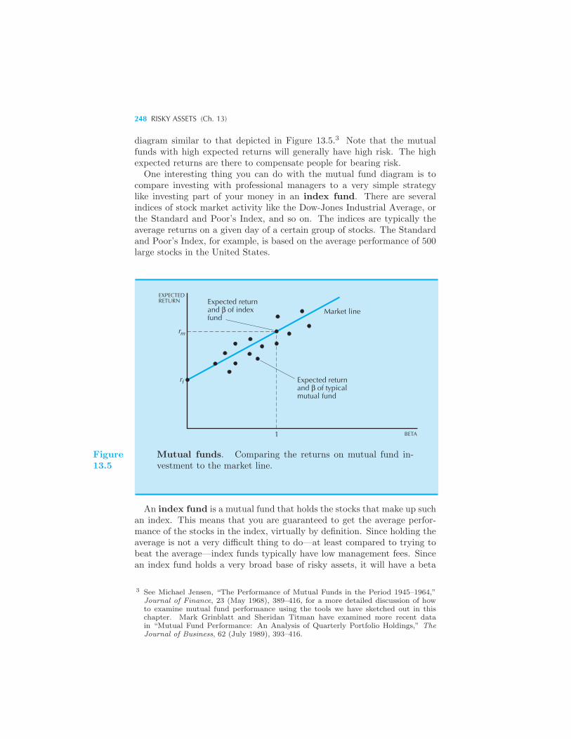
248 RISKY ASSETS (Ch. 13)
diagram similar to that depicted in Figure 13.5.3 Note that the mutualfunds with high expected returns will generally have high risk. The highexpected returns are there to compensate people for bearing risk.One interesting thing you can do with the mutual fund diagram is to
compare investing with professional managers to a very simple strategylike investing part of your money in an index fund. There are severalindices of stock market activity like the Dow-Jones Industrial Average, orthe Standard and Poor’s Index, and so on. The indices are typically theaverage returns on a given day of a certain group of stocks. The Standardand Poor’s Index, for example, is based on the average performance of 500large stocks in the United States.
EXPECTEDRETURN
r
rf
m
Expected returnand β of indexfund
Market line
Expected returnand β of typicalmutual fund
1 BETA
Figure13.5
Mutual funds. Comparing the returns on mutual fund in-vestment to the market line.
An index fund is a mutual fund that holds the stocks that make up suchan index. This means that you are guaranteed to get the average perfor-mance of the stocks in the index, virtually by definition. Since holding theaverage is not a very difficult thing to do—at least compared to trying tobeat the average—index funds typically have low management fees. Sincean index fund holds a very broad base of risky assets, it will have a beta
3 See Michael Jensen, “The Performance of Mutual Funds in the Period 1945–1964,”Journal of Finance, 23 (May 1968), 389–416, for a more detailed discussion of howto examine mutual fund performance using the tools we have sketched out in thischapter. Mark Grinblatt and Sheridan Titman have examined more recent datain “Mutual Fund Performance: An Analysis of Quarterly Portfolio Holdings,” TheJournal of Business, 62 (July 1989), 393–416.
SUMMARY 249
that is very close to 1—it will be just as risky as the market as a whole,because the index fund holds nearly all the stocks in the market as a whole.How does an index fund do as compared to the typical mutual fund?
Remember the comparison has to be made with respect to both risk andreturn of the investment. One way to do this is to plot the expected returnand beta of a Standard and Poor’s Index fund, and draw the line connectingit to the risk-free rate, as in Figure 13.5. You can get any combination ofrisk and return on this line that you want just by deciding how much moneyyou want to invest in the risk-free asset and how much you want to investin the index fund.Now let’s count the number of mutual funds that plot below this line.
These are mutual funds that offer risk and return combinations that aredominated by those available by the index fund/risk-free asset combina-tions. When this is done, it turns out that the vast majority of the risk-return combinations offered by mutual funds are below the line. The num-ber of funds that plot above the line is no more than could be expected bychance alone.But seen another way, this finding might not be too surprising. The stock
market is an incredibly competitive environment. People are always tryingto find undervalued stocks in order to purchase them. This means that onaverage, stocks are usually trading for what they’re really worth. If that isthe case, then betting the averages is a pretty reasonable strategy—sincebeating the averages is almost impossible.
Summary
1. We can use the budget set and indifference curve apparatus developedearlier to examine the choice of how much money to invest in risky andriskless assets.
2. The marginal rate of substitution between risk and return will have toequal the slope of the budget line. This slope is known as the price of risk.
3. The amount of risk present in an asset depends to a large extent on itscorrelation with other assets. An asset that moves opposite the directionof other assets helps to reduce the overall risk of your portfolio.
4. The amount of risk in an asset relative to that of the market as a wholeis called the beta of the asset.
5. The fundamental equilibrium condition in asset markets is that risk-adjusted returns have to be the same.
6. Counterparty risk, which is the risk that the other side of a transactionwill not pay, can also be an important risk factor.
250 RISKY ASSETS (Ch. 13)
REVIEW QUESTIONS
1. If the risk-free rate of return is 6%, and if a risky asset is available witha return of 9% and a standard deviation of 3%, what is the maximum rateof return you can achieve if you are willing to accept a standard deviationof 2%? What percentage of your wealth would have to be invested in therisky asset?
2. What is the price of risk in the above exercise?
3. If a stock has a β of 1.5, the return on the market is 10%, and the risk-free rate of return is 5%, what expected rate of return should this stockoffer according to the Capital Asset Pricing Model? If the expected valueof the stock is $100, what price should the stock be selling for today?
CHAPTER 14
CONSUMER’SSURPLUS
In the preceding chapters we have seen how to derive a consumer’s demandfunction from the underlying preferences or utility function. But in prac-tice we are usually concerned with the reverse problem—how to estimatepreferences or utility from observed demand behavior.We have already examined this problem in two other contexts. In Chap-
ter 5 we showed how one could estimate the parameters of a utility functionfrom observing demand behavior. In the Cobb-Douglas example used inthat chapter, we were able to estimate a utility function that describedthe observed choice behavior simply by calculating the average expendi-ture share of each good. The resulting utility function could then be usedto evaluate changes in consumption.In Chapter 7 we described how to use revealed preference analysis to
recover estimates of the underlying preferences that may have generatedsome observed choices. These estimated indifference curves can also beused to evaluate changes in consumption.In this chapter we will consider some more approaches to the problem
of estimating utility from observing demand behavior. Although some ofthe methods we will examine are less general than the two methods we
252 CONSUMER’S SURPLUS (Ch. 14)
examined previously, they will turn out to be useful in several applicationsthat we will discuss later in the book.We will start by reviewing a special case of demand behavior for which
it is very easy to recover an estimate of utility. Later we will consider moregeneral cases of preferences and demand behavior.
14.1 Demand for a Discrete Good
Let us start by reviewing demand for a discrete good with quasilinearutility, as described in Chapter 6. Suppose that the utility function takesthe form v(x)+ y and that the x-good is only available in integer amounts.Let us think of the y-good as money to be spent on other goods and set itsprice to 1. Let p be the price of the x-good.We saw in Chapter 6 that in this case consumer behavior can be described
in terms of the reservation prices, r1 = v(1) − v(0), r2 = v(2) − v(1), andso on. The relationship between reservation prices and demand was verysimple: if n units of the discrete good are demanded, then rn ≥ p ≥ rn+1.To verify this, let’s look at an example. Suppose that the consumer
chooses to consume 6 units of the x-good when its price is p. Then theutility of consuming (6,m − 6p) must be at least as large as the utility ofconsuming any other bundle (x,m− px):
v(6) +m− 6p ≥ v(x) +m− px. (14.1)
In particular this inequality must hold for x = 5, which gives us
v(6) +m− 6p ≥ v(5) +m− 5p.
Rearranging, we have v(6)− v(5) = r6 ≥ p.Equation (14.1) must also hold for x = 7. This gives us
v(6) +m− 6p ≥ v(7) +m− 7p,
which can be rearranged to yield
p ≥ v(7)− v(6) = r7.
This argument shows that if 6 units of the x-good is demanded, then theprice of the x-good must lie between r6 and r7. In general, if n units ofthe x-good are demanded at price p, then rn ≥ p ≥ rn+1, as we wanted toshow. The list of reservation prices contains all the information necessary todescribe the demand behavior. The graph of the reservation prices forms a“staircase” as shown in Figure 14.1. This staircase is precisely the demandcurve for the discrete good.
CONSTRUCTING UTILITY FROM DEMAND 253
14.2 Constructing Utility from Demand
We have just seen how to construct the demand curve given the reservationprices or the utility function. But we can also do the same operation inreverse. If we are given the demand curve, we can construct the utilityfunction—at least in the special case of quasilinear utility.At one level, this is just a trivial operation of arithmetic. The reservation
prices are defined to be the difference in utility:
r1 = v(1)− v(0)
r2 = v(2)− v(1)
r3 = v(3)− v(2)
...
If we want to calculate v(3), for example, we simply add up both sides ofthis list of equations to find
r1 + r2 + r3 = v(3)− v(0).
It is convenient to set the utility from consuming zero units of the goodequal to zero, so that v(0) = 0, and therefore v(n) is just the sum of thefirst n reservation prices.This construction has a nice geometrical interpretation that is illustrated
in Figure 14.1A. The utility from consuming n units of the discrete good isjust the area of the first n bars which make up the demand function. Thisis true because the height of each bar is the reservation price associatedwith that level of demand and the width of each bar is 1. This area issometimes called the gross benefit or the gross consumer’s surplusassociated with the consumption of the good.Note that this is only the utility associated with the consumption of
good 1. The final utility of consumption depends on the how much theconsumer consumes of good 1 and good 2. If the consumer chooses n unitsof the discrete good, then he will have m− pn dollars left over to purchaseother things. This leaves him with a total utility of
v(n) +m− pn.
This utility also has an interpretation as an area: we just take the areadepicted in Figure 14.1A, subtract off the expenditure on the discrete good,and add m.
The term v(n) − pn is called consumer’s surplus or the net con-sumer’s surplus. It measures the net benefits from consuming n units ofthe discrete good: the utility v(n) minus the reduction in the expenditureon consumption of the other good. The consumer’s surplus is depicted inFigure 14.1B.
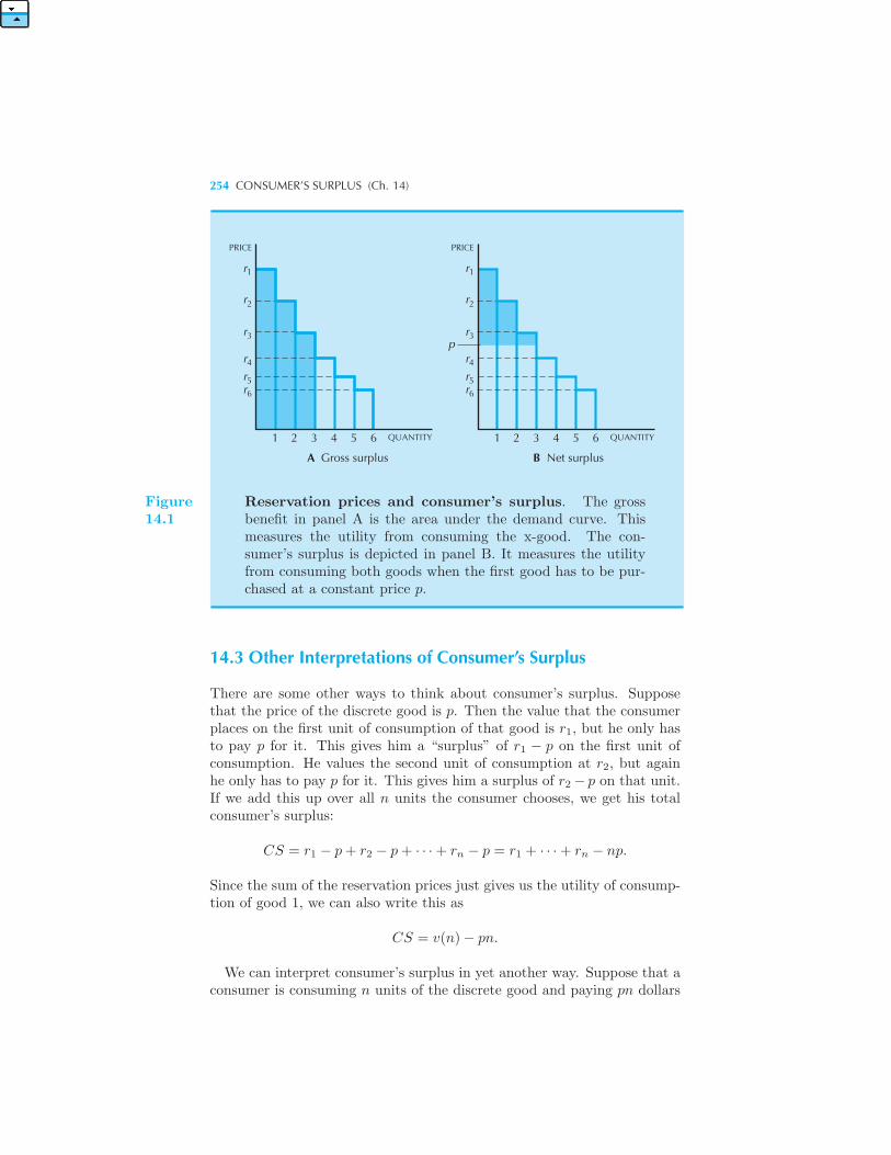
254 CONSUMER’S SURPLUS (Ch. 14)
r
r
r
r
rr
1
2
3
4
5
6
PRICE
1 2 3 4 5 6 QUANTITY
A Gross surplus
r
r
r
r
rr
1
2
3
4
5
6
PRICE
1 2 3 4 5 6 QUANTITY
B Net surplus
p
Figure14.1
Reservation prices and consumer’s surplus. The grossbenefit in panel A is the area under the demand curve. Thismeasures the utility from consuming the x-good. The con-sumer’s surplus is depicted in panel B. It measures the utilityfrom consuming both goods when the first good has to be pur-chased at a constant price p.
14.3 Other Interpretations of Consumer’s Surplus
There are some other ways to think about consumer’s surplus. Supposethat the price of the discrete good is p. Then the value that the consumerplaces on the first unit of consumption of that good is r1, but he only hasto pay p for it. This gives him a “surplus” of r1 − p on the first unit ofconsumption. He values the second unit of consumption at r2, but againhe only has to pay p for it. This gives him a surplus of r2 − p on that unit.If we add this up over all n units the consumer chooses, we get his totalconsumer’s surplus:
CS = r1 − p+ r2 − p+ · · ·+ rn − p = r1 + · · ·+ rn − np.
Since the sum of the reservation prices just gives us the utility of consump-tion of good 1, we can also write this as
CS = v(n)− pn.
We can interpret consumer’s surplus in yet another way. Suppose that aconsumer is consuming n units of the discrete good and paying pn dollars
QUASILINEAR UTILITY 255
to do so. How much money would he need to induce him to give up hisentire consumption of this good? Let R be the required amount of money.Then R must satisfy the equation
v(0) +m+R = v(n) +m− pn.
Since v(0) = 0 by definition, this equation reduces to
R = v(n)− pn,
which is just consumer’s surplus. Hence the consumer’s surplus measureshow much a consumer would need to be paid to give up his entire con-sumption of some good.
14.4 From Consumer’s Surplus to Consumers’ Surplus
Up until now we have been considering the case of a single consumer. If sev-eral consumers are involved we can add up each consumer’s surplus acrossall the consumers to create an aggregate measure of the consumers’ sur-plus. Note carefully the distinction between the two concepts: consumer’ssurplus refers to the surplus of a single consumer; consumers’ surplus refersto the sum of the surpluses across a number of consumers.Consumers’ surplus serves as a convenient measure of the aggregate gains
from trade, just as consumer’s surplus serves as a measure of the individualgains from trade.
14.5 Approximating a Continuous Demand
We have seen that the area underneath the demand curve for a discretegood measures the utility of consumption of that good. We can extend thisto the case of a good available in continuous quantities by approximatingthe continuous demand curve by a staircase demand curve. The area underthe continuous demand curve is then approximately equal to the area underthe staircase demand.See Figure 14.2 for an example. In the Appendix to this chapter we show
how to use calculus to calculate the exact area under a demand curve.
14.6 Quasilinear Utility
It is worth thinking about the role that quasilinear utility plays in thisanalysis. In general the price at which a consumer is willing to purchase
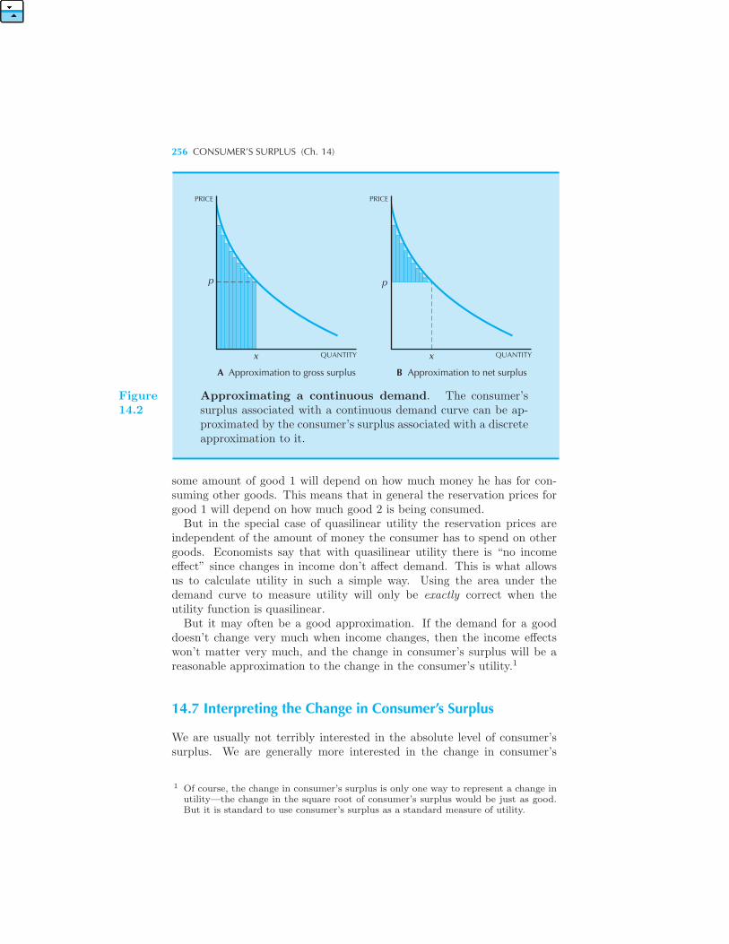
256 CONSUMER’S SURPLUS (Ch. 14)
PRICE PRICE
p
x QUANTITY QUANTITY
p
x
A Approximation to gross surplus B Approximation to net surplus
Figure14.2
Approximating a continuous demand. The consumer’ssurplus associated with a continuous demand curve can be ap-proximated by the consumer’s surplus associated with a discreteapproximation to it.
some amount of good 1 will depend on how much money he has for con-suming other goods. This means that in general the reservation prices forgood 1 will depend on how much good 2 is being consumed.But in the special case of quasilinear utility the reservation prices are
independent of the amount of money the consumer has to spend on othergoods. Economists say that with quasilinear utility there is “no incomeeffect” since changes in income don’t affect demand. This is what allowsus to calculate utility in such a simple way. Using the area under thedemand curve to measure utility will only be exactly correct when theutility function is quasilinear.But it may often be a good approximation. If the demand for a good
doesn’t change very much when income changes, then the income effectswon’t matter very much, and the change in consumer’s surplus will be areasonable approximation to the change in the consumer’s utility.1
14.7 Interpreting the Change in Consumer’s Surplus
We are usually not terribly interested in the absolute level of consumer’ssurplus. We are generally more interested in the change in consumer’s
1 Of course, the change in consumer’s surplus is only one way to represent a change inutility—the change in the square root of consumer’s surplus would be just as good.But it is standard to use consumer’s surplus as a standard measure of utility.
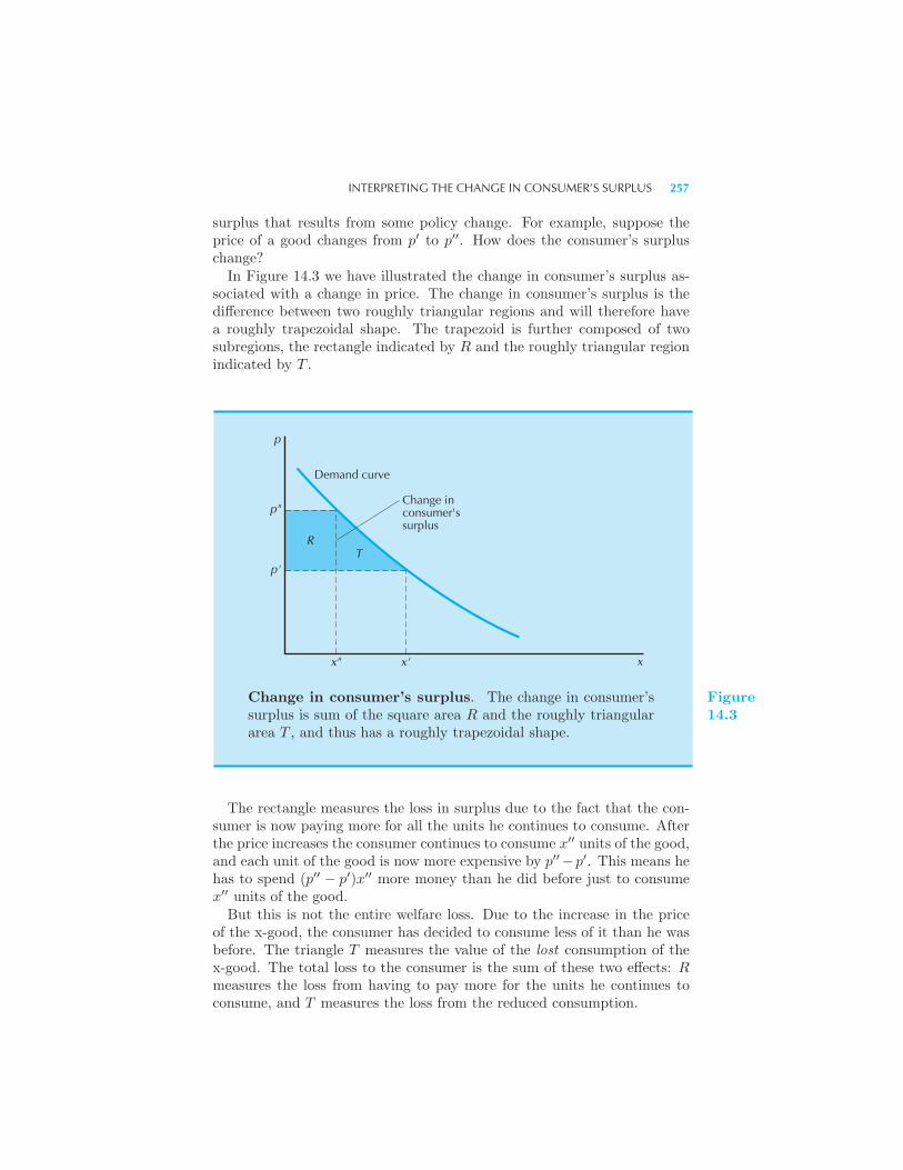
INTERPRETING THE CHANGE IN CONSUMER’S SURPLUS 257
surplus that results from some policy change. For example, suppose theprice of a good changes from p′ to p′′. How does the consumer’s surpluschange?In Figure 14.3 we have illustrated the change in consumer’s surplus as-
sociated with a change in price. The change in consumer’s surplus is thedifference between two roughly triangular regions and will therefore havea roughly trapezoidal shape. The trapezoid is further composed of twosubregions, the rectangle indicated by R and the roughly triangular regionindicated by T .
Demand curve
Change inconsumer'ssurplus
p
p"
p'
RT
x" x' x
Change in consumer’s surplus. The change in consumer’ssurplus is sum of the square area R and the roughly triangulararea T , and thus has a roughly trapezoidal shape.
Figure14.3
The rectangle measures the loss in surplus due to the fact that the con-sumer is now paying more for all the units he continues to consume. Afterthe price increases the consumer continues to consume x′′ units of the good,and each unit of the good is now more expensive by p′′−p′. This means hehas to spend (p′′ − p′)x′′ more money than he did before just to consumex′′ units of the good.But this is not the entire welfare loss. Due to the increase in the price
of the x-good, the consumer has decided to consume less of it than he wasbefore. The triangle T measures the value of the lost consumption of thex-good. The total loss to the consumer is the sum of these two effects: Rmeasures the loss from having to pay more for the units he continues toconsume, and T measures the loss from the reduced consumption.
258 CONSUMER’S SURPLUS (Ch. 14)
EXAMPLE: The Change in Consumer’s Surplus
Question: Consider the linear demand curve D(p) = 20 − 2p. When theprice changes from 2 to 3 what is the associated change in consumer’ssurplus?
Answer: When p = 2, D(2) = 16, and when p = 3, D(3) = 14. Thus wewant to compute the area of a trapezoid with a height of 1 and bases of 14and 16. This is equivalent to a rectangle with height 1 and base 14 (havingan area of 14), plus a triangle of height 1 and base 2 (having an area of 1).The total area will therefore be 15.
14.8 Compensating and Equivalent Variation
The theory of consumer’s surplus is very tidy in the case of quasilinearutility. Even if utility is not quasilinear, consumer’s surplus may still bea reasonable measure of consumer’s welfare in many applications. Usuallythe errors in measuring demand curves outweigh the approximation errorsfrom using consumer’s surplus.But it may be that for some applications an approximation may not
be good enough. In this section we’ll outline a way to measure “utilitychanges” without using consumer’s surplus. There are really two separateissues involved. The first has to do with how to estimate utility when wecan observe a number of consumer choices. The second has to do with howwe can measure utility in monetary units.We’ve already investigated the estimation problem. We gave an example
of how to estimate a Cobb-Douglas utility function in Chapter 6. In thatexample we noticed that expenditure shares were relatively constant andthat we could use the average expenditure share as estimates of the Cobb-Douglas parameters. If the demand behavior didn’t exhibit this particularfeature, we would have to choose a more complicated utility function, butthe principle would be just the same: if we have enough observations ondemand behavior and that behavior is consistent with maximizing some-thing, then we will generally be able to estimate the function that is beingmaximized.Once we have an estimate of the utility function that describes some
observed choice behavior we can use this function to evaluate the impactof proposed changes in prices and consumption levels. At the most funda-mental level of analysis, this is the best we can hope for. All that mattersare the consumer’s preferences; any utility function that describes the con-sumer’s preferences is as good as any other.However, in some applications it may be convenient to use certain mon-
etary measures of utility. For example, we could ask how much money we
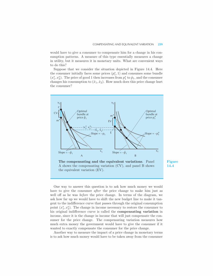
COMPENSATING AND EQUIVALENT VARIATION 259
would have to give a consumer to compensate him for a change in his con-sumption patterns. A measure of this type essentially measures a changein utility, but it measures it in monetary units. What are convenient waysto do this?Suppose that we consider the situation depicted in Figure 14.4. Here
the consumer initially faces some prices (p∗1, 1) and consumes some bundle(x∗
1, x∗2). The price of good 1 then increases from p∗1 to p1, and the consumer
changes his consumption to (x1, x2). How much does this price change hurtthe consumer?
Optimalbundle atprice p1
Slope = –p1
x1
{CV
C
(x1, x2)^ ^(x1, x2 )* *
{
Slope = –p1
x2
x1
A
m*
{EV
E
B
Slope = –p1*
Optimalbundle atprice p1
*
Slope = –p1
m*
x2
The compensating and the equivalent variations. PanelA shows the compensating variation (CV), and panel B showsthe equivalent variation (EV).
Figure14.4
One way to answer this question is to ask how much money we wouldhave to give the consumer after the price change to make him just aswell off as he was before the price change. In terms of the diagram, weask how far up we would have to shift the new budget line to make it tan-gent to the indifference curve that passes through the original consumptionpoint (x∗
1, x∗2). The change in income necessary to restore the consumer to
his original indifference curve is called the compensating variation inincome, since it is the change in income that will just compensate the con-sumer for the price change. The compensating variation measures howmuch extra money the government would have to give the consumer if itwanted to exactly compensate the consumer for the price change.Another way to measure the impact of a price change in monetary terms
is to ask how much money would have to be taken away from the consumer
260 CONSUMER’S SURPLUS (Ch. 14)
before the price change to leave him as well off as he would be after theprice change. This is called the equivalent variation in income since itis the income change that is equivalent to the price change in terms ofthe change in utility. In Figure 14.4 we ask how far down we must shiftthe original budget line to just touch the indifference curve that passesthrough the new consumption bundle. The equivalent variation measuresthe maximum amount of income that the consumer would be willing to payto avoid the price change.In general the amount of money that the consumer would be willing
to pay to avoid a price change would be different from the amount ofmoney that the consumer would have to be paid to compensate him fora price change. After all, at different sets of prices a dollar is worth adifferent amount to a consumer since it will purchase different amounts ofconsumption.In geometric terms, the compensating and equivalent variations are just
two different ways to measure “how far apart” two indifference curves are.In each case we are measuring the distance between two indifference curvesby seeing how far apart their tangent lines are. In general this measureof distance will depend on the slope of the tangent lines—that is, on theprices that we choose to determine the budget lines.However, the compensating and equivalent variation are the same in one
important case—the case of quasilinear utility. In this case the indifferencecurves are parallel, so the distance between any two indifference curves isthe same no matter where it is measured, as depicted in Figure 14.5. Inthe case of quasilinear utility the compensating variation, the equivalentvariation, and the change in consumer’s surplus all give the same measureof the monetary value of a price change.
EXAMPLE: Compensating and Equivalent Variations
Suppose that a consumer has a utility function u(x1, x2) = x121 x
122 . He
originally faces prices (1, 1) and has income 100. Then the price of good 1increases to 2. What are the compensating and equivalent variations?We know that the demand functions for this Cobb-Douglas utility func-
tion are given by
x1 =m
2p1
x2 =m
2p2.
Using this formula, we see that the consumer’s demands change from(x∗
1, x∗2) = (50, 50) to (x1, x2) = (25, 50).
To calculate the compensating variation we ask how much money wouldbe necessary at prices (2,1) to make the consumer as well off as he wasconsuming the bundle (50,50)? If the prices were (2,1) and the consumer
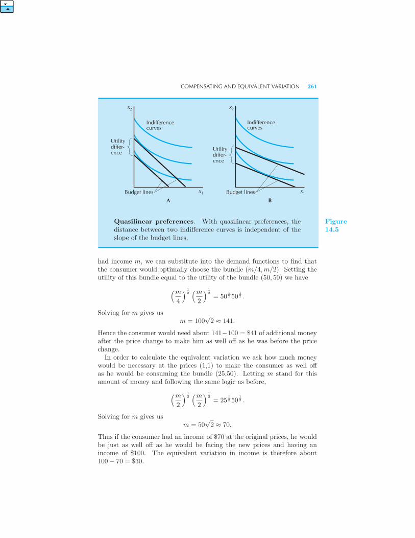
COMPENSATING AND EQUIVALENT VARIATION 261
x2
Indifferencecurves
Budget lines x1 1Budget lines
Indifferencecurves
2x
A B
Utilitydiffer-ence
Utilitydiffer-ence
x
Quasilinear preferences. With quasilinear preferences, thedistance between two indifference curves is independent of theslope of the budget lines.
Figure14.5
had income m, we can substitute into the demand functions to find thatthe consumer would optimally choose the bundle (m/4,m/2). Setting theutility of this bundle equal to the utility of the bundle (50, 50) we have
(m4
) 12(m2
) 12
= 5012 50
12 .
Solving for m gives usm = 100
√2 ≈ 141.
Hence the consumer would need about 141−100 = $41 of additional moneyafter the price change to make him as well off as he was before the pricechange.In order to calculate the equivalent variation we ask how much money
would be necessary at the prices (1,1) to make the consumer as well offas he would be consuming the bundle (25,50). Letting m stand for thisamount of money and following the same logic as before,
(m2
) 12(m2
) 12
= 2512 50
12 .
Solving for m gives usm = 50
√2 ≈ 70.
Thus if the consumer had an income of $70 at the original prices, he wouldbe just as well off as he would be facing the new prices and having anincome of $100. The equivalent variation in income is therefore about100− 70 = $30.
262 CONSUMER’S SURPLUS (Ch. 14)
EXAMPLE: Compensating and Equivalent Variation for QuasilinearPreferences
Suppose that the consumer has a quasilinear utility function v(x1) + x2.We know that in this case the demand for good 1 will depend only on theprice of good 1, so we write it as x1(p1). Suppose that the price changesfrom p∗1 to p1. What are the compensating and equivalent variations?At the price p∗1, the consumer chooses x∗
1 = x1(p∗1) and has a utility of
v(x∗1) +m − p∗1x
∗1. At the price p1, the consumer choose x1 = x1(p1) and
has a utility of v(x1) +m− p1x1.Let C be the compensating variation. This is the amount of extra money
the consumer would need after the price change to make him as well off ashe would be before the price change. Setting these utilities equal we have
v(x1) +m+ C − p1x1 = v(x∗1) +m− p∗1x
∗1.
Solving for C we have
C = v(x∗1)− v(x1) + p1x1 − p∗1x
∗1.
Let E be the equivalent variation. This is the amount of money thatyou could take away from the consumer before the price change that wouldleave him with the same utility that he would have after the price change.Thus it satisfies the equation
v(x∗1) +m− E − p∗1x
∗1 = v(x1) +m− p1x1.
Solving for E, we have
E = v(x∗1)− v(x1) + p1x1 − p∗1x
∗1.
Note that for the case of quasilinear utility the compensating and equiv-alent variation are the same. Furthermore, they are both equal to thechange in (net) consumer’s surplus:
ΔCS = [v(x∗1)− p∗1x
∗1]− [v(x1)− p1x1].
14.9 Producer’s Surplus
The demand curve measures the amount that will be demanded at eachprice; the supply curve measures the amount that will be supplied at
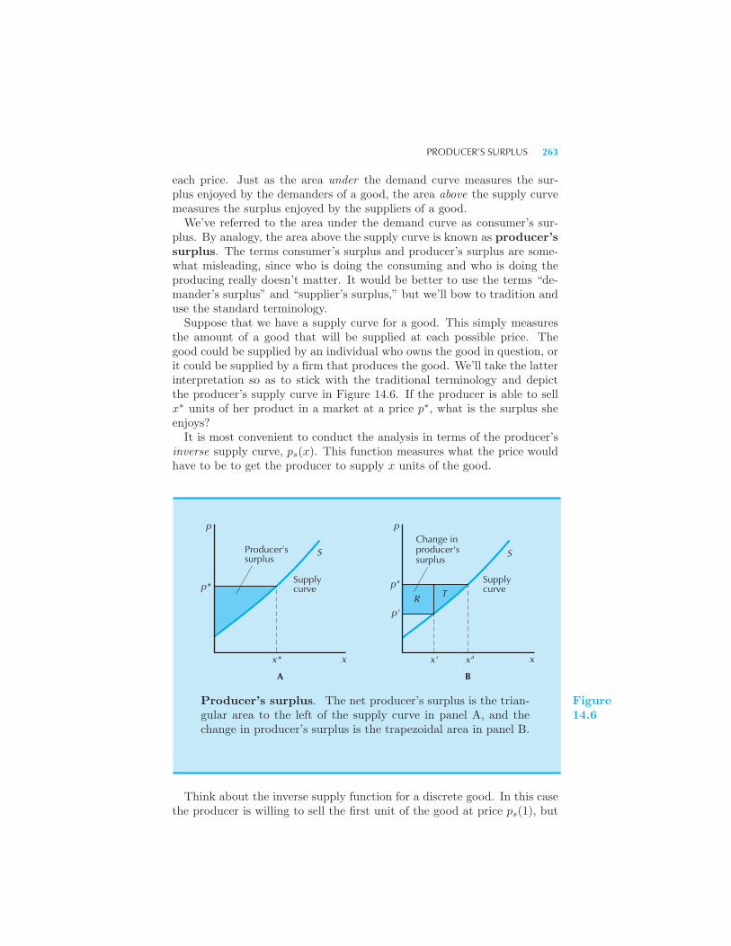
PRODUCER’S SURPLUS 263
each price. Just as the area under the demand curve measures the sur-plus enjoyed by the demanders of a good, the area above the supply curvemeasures the surplus enjoyed by the suppliers of a good.We’ve referred to the area under the demand curve as consumer’s sur-
plus. By analogy, the area above the supply curve is known as producer’ssurplus. The terms consumer’s surplus and producer’s surplus are some-what misleading, since who is doing the consuming and who is doing theproducing really doesn’t matter. It would be better to use the terms “de-mander’s surplus” and “supplier’s surplus,” but we’ll bow to tradition anduse the standard terminology.Suppose that we have a supply curve for a good. This simply measures
the amount of a good that will be supplied at each possible price. Thegood could be supplied by an individual who owns the good in question, orit could be supplied by a firm that produces the good. We’ll take the latterinterpretation so as to stick with the traditional terminology and depictthe producer’s supply curve in Figure 14.6. If the producer is able to sellx∗ units of her product in a market at a price p∗, what is the surplus sheenjoys?It is most convenient to conduct the analysis in terms of the producer’s
inverse supply curve, ps(x). This function measures what the price wouldhave to be to get the producer to supply x units of the good.
p
p*
p
x x
S S
x* x' x"
p'
p"
A B
Supplycurve
R T
Change inproducer'ssurplus
Supplycurve
Producer'ssurplus
Producer’s surplus. The net producer’s surplus is the trian-gular area to the left of the supply curve in panel A, and thechange in producer’s surplus is the trapezoidal area in panel B.
Figure14.6
Think about the inverse supply function for a discrete good. In this casethe producer is willing to sell the first unit of the good at price ps(1), but
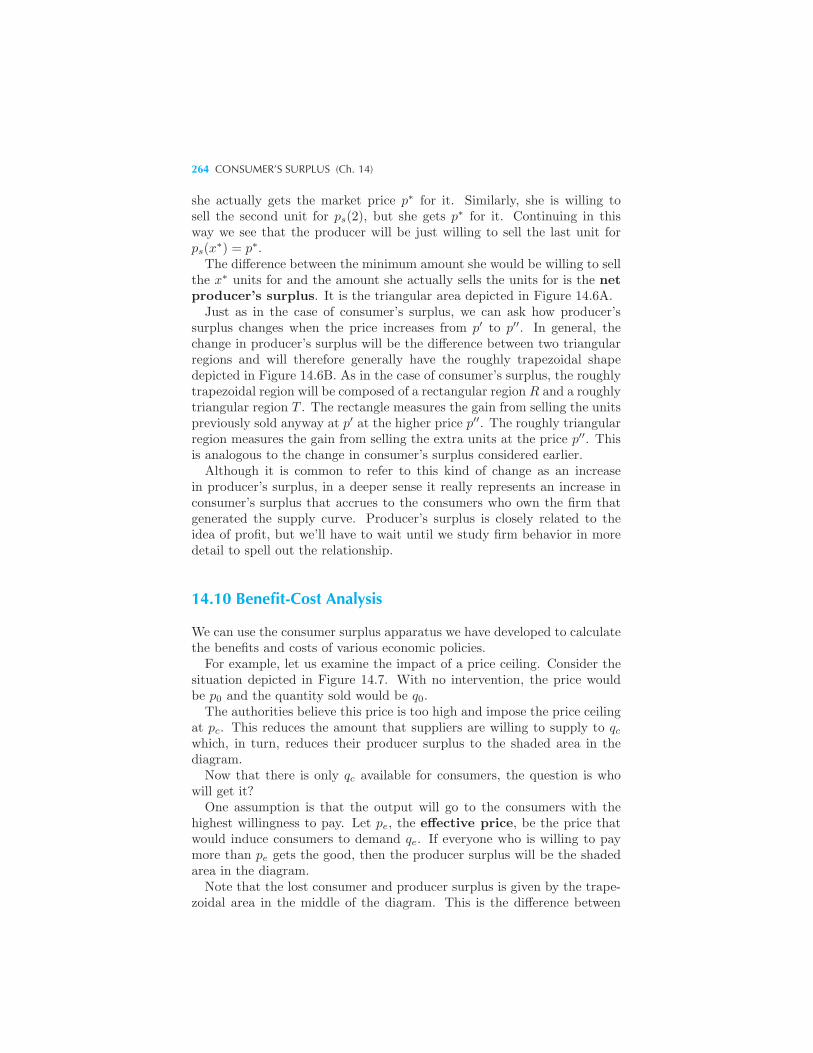
264 CONSUMER’S SURPLUS (Ch. 14)
she actually gets the market price p∗ for it. Similarly, she is willing tosell the second unit for ps(2), but she gets p∗ for it. Continuing in thisway we see that the producer will be just willing to sell the last unit forps(x
∗) = p∗.The difference between the minimum amount she would be willing to sell
the x∗ units for and the amount she actually sells the units for is the netproducer’s surplus. It is the triangular area depicted in Figure 14.6A.Just as in the case of consumer’s surplus, we can ask how producer’s
surplus changes when the price increases from p′ to p′′. In general, thechange in producer’s surplus will be the difference between two triangularregions and will therefore generally have the roughly trapezoidal shapedepicted in Figure 14.6B. As in the case of consumer’s surplus, the roughlytrapezoidal region will be composed of a rectangular region R and a roughlytriangular region T . The rectangle measures the gain from selling the unitspreviously sold anyway at p′ at the higher price p′′. The roughly triangularregion measures the gain from selling the extra units at the price p′′. Thisis analogous to the change in consumer’s surplus considered earlier.Although it is common to refer to this kind of change as an increase
in producer’s surplus, in a deeper sense it really represents an increase inconsumer’s surplus that accrues to the consumers who own the firm thatgenerated the supply curve. Producer’s surplus is closely related to theidea of profit, but we’ll have to wait until we study firm behavior in moredetail to spell out the relationship.
14.10 Benefit-Cost Analysis
We can use the consumer surplus apparatus we have developed to calculatethe benefits and costs of various economic policies.For example, let us examine the impact of a price ceiling. Consider the
situation depicted in Figure 14.7. With no intervention, the price wouldbe p0 and the quantity sold would be q0.
The authorities believe this price is too high and impose the price ceilingat pc. This reduces the amount that suppliers are willing to supply to qcwhich, in turn, reduces their producer surplus to the shaded area in thediagram.Now that there is only qc available for consumers, the question is who
will get it?One assumption is that the output will go to the consumers with the
highest willingness to pay. Let pe, the effective price, be the price thatwould induce consumers to demand qe. If everyone who is willing to paymore than pe gets the good, then the producer surplus will be the shadedarea in the diagram.Note that the lost consumer and producer surplus is given by the trape-
zoidal area in the middle of the diagram. This is the difference between
BENEFIT-COST ANALYSIS 265
Supplycurve
pe
Demandcurve
QUANTITY
CS
PS
p0
pc
qc = qe q0
PRICE
A price ceiling. The price ceiling at pc reduces supply toqe. It reduces consumer surplus to CS and producer surplus toPS. The effective price of the good, pe, is the price that wouldclear the market. The diagram also shows what happens withrationing, in which case the price of a ration coupon would bepe − pc.
Figure14.7
the consumer plus producer surplus in the competitive market and thedifference in the market with the price ceiling.
Assuming that the quantity will go to consumers with the highest will-ingness to pay is overly optimistic in most situation. Hence, we we wouldgenerally expect that this trapezoidal area is a lower bound on the lostconsumer plus producer surplus in the case of a price ceiling.
Rationing
The diagram we have just examined can also be used to describe the sociallosses due to rationing. Instead of fixing a price ceiling of pc, supposethat the authorities issue ration coupons that allow for only qc units to bepurchased. In order to purchase one unit of the good, a consumer needs topay pc to the seller and produce a ration coupon.
If the ration coupons are marketable, then they would sell for a price ofpe − pc. This would make the the total price of the purchase equal to pe,which is the price that clears the market for the good being sold.
266 CONSUMER’S SURPLUS (Ch. 14)
14.11 Calculating Gains and Losses
If we have estimates of the market demand and supply curves for a good,it is not difficult in principle to calculate the loss in consumers’ surplus dueto changes in government policies. For example, suppose the governmentdecides to change its tax treatment of some good. This will result in achange in the prices that consumers face and therefore a change in theamount of the good that they will choose to consume. We can calculate theconsumers’ surplus associated with different tax proposals and see whichtax reforms generate the smallest loss.This is often useful information for judging various methods of taxation,
but it suffers from two defects. First, as we’ve indicated earlier, the con-sumer’s surplus calculation is only valid for special forms of preferences—namely, preferences representable by a quasilinear utility function. Weargued earlier that this kind of utility function may be a reasonable ap-proximation for goods for which changes in income lead to small changesin demand, but for goods whose consumption is closely related to income,the use of consumer surplus may be inappropriate.Second, the calculation of this loss effectively lumps together all the
consumers and producers and generates an estimate of the “cost” of asocial policy only for some mythical “representative consumer.” In manycases it is desirable to know not only the average cost across the population,but who bears the costs. The political success or failure of policies oftendepends more on the distribution of gains and losses than on the averagegain or loss.Consumer’s surplus may be easy to calculate, but we’ve seen that it is
not that much more difficult to calculate the true compensating or equiv-alent variation associated with a price change. If we have estimates of thedemand functions of each household—or at least the demand functions fora sample of representative households—we can calculate the impact of apolicy change on each household in terms of the compensating or equiva-lent variation. Thus we will have a measure of the “benefits” or “costs”imposed on each household by the proposed policy change.Mervyn King, an economist at the London School of Economics, has
described a nice example of this approach to analyzing the implicationsof reforming the tax treatment of housing in Britain in his paper “Wel-fare Analysis of Tax Reforms Using Household Data,” Journal of PublicEconomics, 21 (1983), 183–214.King first examined the housing expenditures of 5,895 households and
estimated a demand function that best described their purchases of hous-ing services. Next, he used this demand function to determine a utilityfunction for each household. Finally, he used the estimated utility functionto calculate how much each household would gain or lose under certainchanges in the taxation of housing in Britain. The measure that he used
REVIEW QUESTIONS 267
was similar to the equivalent variation described earlier in this chapter.The basic nature of the tax reform he studied was to eliminate tax con-cessions to owner-occupied housing and to raise rents in public housing.The revenues generated by these changes would be handed back to thehouseholds in the form of transfers proportional to household income.King found that 4,888 of the 5,895 households would benefit from this
kind of reform. More importantly he could identify explicitly those house-holds that would have significant losses from the tax reform. King found,for example, that 94 percent of the highest income households gained fromthe reform, while only 58 percent of the lowest income households gained.This kind of information would allow special measures to be undertakenwhich might help in designing the tax reform in a way that could satisfydistributional objectives.
Summary
1. In the case of a discrete good and quasilinear utility, the utility associ-ated with the consumption of n units of the discrete good is just the sumof the first n reservation prices.
2. This sum is the gross benefit of consuming the good. If we subtract theamount spent on the purchase of the good, we get the consumer’s surplus.
3. The change in consumer’s surplus associated with a price change has aroughly trapezoidal shape. It can be interpreted as the change in utilityassociated with the price change.
4. In general, we can use the compensating variation and the equivalentvariation in income to measure the monetary impact of a price change.
5. If utility is quasilinear, the compensating variation, the equivalent vari-ation, and the change in consumer’s surplus are all equal. Even if utilityis not quasilinear, the change in consumer’s surplus may serve as a goodapproximation of the impact of the price change on a consumer’s utility.
6. In the case of supply behavior we can define a producer’s surplus thatmeasures the net benefits to the supplier from producing a given amountof output.
REVIEW QUESTIONS
1. A good can be produced in a competitive industry at a cost of $10 perunit. There are 100 consumers are each willing to pay $12 each to consume
268 CONSUMER’S SURPLUS (Ch. 14)
a single unit of the good (additional units have no value to them.) Whatis the equilibrium price and quantity sold? The government imposes a taxof $1 on the good. What is the deadweight loss of this tax?
2. Suppose that the demand curve is given by D(p) = 10− p. What is thegross benefit from consuming 6 units of the good?
3. In the above example, if the price changes from 4 to 6, what is the changein consumer’s surplus?
4. Suppose that a consumer is consuming 10 units of a discrete good andthe price increases from $5 per unit to $6. However, after the price changethe consumer continues to consume 10 units of the discrete good. What isthe loss in the consumer’s surplus from this price change?
APPENDIX
Let’s use some calculus to treat consumer’s surplus rigorously. Start with theproblem of maximizing quasilinear utility:
maxx,y
v(x) + y
such that px+ y = m.
Substituting from the budget constraint we have
maxx
v(x) +m− px.
The first-order condition for this problem is
v′(x) = p.
This means that the inverse demand function p(x) is defined by
p(x) = v′(x). (14.2)
Note the analogy with the discrete-good framework described in the text: theprice at which the consumer is just willing to consume x units is equal to themarginal utility.
But since the inverse demand curve measures the derivative of utility, we cansimply integrate under the inverse demand function to find the utility function.
Carrying out the integration we have:
v(x) = v(x)− v(0) =
∫ x
0
v′(t) dt =
∫ x
0
p(t) dt.
Hence utility associated with the consumption of the x-good is just the area underthe demand curve.
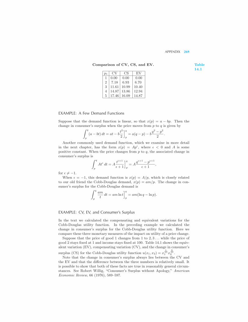
APPENDIX 269
Table14.1
Comparison of CV, CS, and EV.
p1 CV CS EV
1 0.00 0.00 0.002 7.18 6.93 6.703 11.61 10.99 10.404 14.87 13.86 12.945 17.46 16.09 14.87
EXAMPLE: A Few Demand Functions
Suppose that the demand function is linear, so that x(p) = a − bp. Then thechange in consumer’s surplus when the price moves from p to q is given by∫ q
p
(a− bt) dt = at− bt2
2
]qp= a(q − p)− b
q2 − p2
2.
Another commonly used demand function, which we examine in more detailin the next chapter, has the form x(p) = Apε, where ε < 0 and A is somepositive constant. When the price changes from p to q, the associated change inconsumer’s surplus is∫ q
p
Atε dt = Atε+1
ε+ 1
]qp= A
qε+1 − pε+1
ε+ 1,
for ε �= −1.When ε = −1, this demand function is x(p) = A/p, which is closely related
to our old friend the Cobb-Douglas demand, x(p) = am/p. The change in con-sumer’s surplus for the Cobb-Douglas demand is∫ q
p
am
tdt = am ln t
]qp= am(ln q − ln p).
EXAMPLE: CV, EV, and Consumer’s Surplus
In the text we calculated the compensating and equivalent variations for theCobb-Douglas utility function. In the preceding example we calculated thechange in consumer’s surplus for the Cobb-Douglas utility function. Here wecompare these three monetary measures of the impact on utility of a price change.
Suppose that the price of good 1 changes from 1 to 2, 3 . . . while the price ofgood 2 stays fixed at 1 and income stays fixed at 100. Table 14.1 shows the equiv-alent variation (EV), compensating variation (CV), and the change in consumer’s
surplus (CS) for the Cobb-Douglas utility function u(x1, x2) = x1101 x
9102 .
Note that the change in consumer’s surplus always lies between the CV andthe EV and that the difference between the three numbers is relatively small. Itis possible to show that both of these facts are true in reasonably general circum-stances. See Robert Willig, “Consumer’s Surplus without Apology,” AmericanEconomic Review, 66 (1976), 589–597.
CHAPTER 15
MARKETDEMAND
We have seen in earlier chapters how to model individual consumer choice.Here we see how to add up individual choices to get totalmarket demand.Once we have derived the market demand curve, we will examine some ofits properties, such as the relationship between demand and revenue.
15.1 From Individual to Market Demand
Let us use x1i (p1, p2,mi) to represent consumer i’s demand function for
good 1 and x2i (p1, p2,mi) for consumer i’s demand function for good 2.
Suppose that there are n consumers. Then the market demand for good1, also called the aggregate demand for good 1, is the sum of theseindividual demands over all consumers:
X1(p1, p2,m1, . . . ,mn) =n∑
i=1
x1i (p1, p2,mi).
The analogous equation holds for good 2.
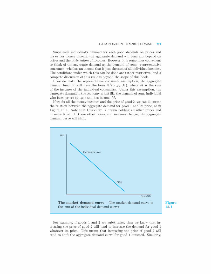
FROM INDIVIDUAL TO MARKET DEMAND 271
Since each individual’s demand for each good depends on prices andhis or her money income, the aggregate demand will generally depend onprices and the distribution of incomes. However, it is sometimes convenientto think of the aggregate demand as the demand of some “representativeconsumer” who has an income that is just the sum of all individual incomes.The conditions under which this can be done are rather restrictive, and acomplete discussion of this issue is beyond the scope of this book.If we do make the representative consumer assumption, the aggregate
demand function will have the form X1(p1, p2,M), where M is the sumof the incomes of the individual consumers. Under this assumption, theaggregate demand in the economy is just like the demand of some individualwho faces prices (p1, p2) and has income M .If we fix all the money incomes and the price of good 2, we can illustrate
the relation between the aggregate demand for good 1 and its price, as inFigure 15.1. Note that this curve is drawn holding all other prices andincomes fixed. If these other prices and incomes change, the aggregatedemand curve will shift.
QUANTITY
PRICE
Demand curve
D (p)
The market demand curve. The market demand curve isthe sum of the individual demand curves.
Figure15.1
For example, if goods 1 and 2 are substitutes, then we know that in-creasing the price of good 2 will tend to increase the demand for good 1whatever its price. This means that increasing the price of good 2 willtend to shift the aggregate demand curve for good 1 outward. Similarly,
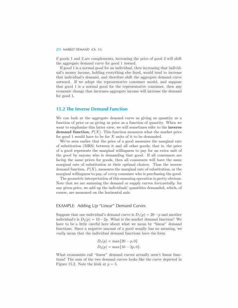
272 MARKET DEMAND (Ch. 15)
if goods 1 and 2 are complements, increasing the price of good 2 will shiftthe aggregate demand curve for good 1 inward.If good 1 is a normal good for an individual, then increasing that individ-
ual’s money income, holding everything else fixed, would tend to increasethat individual’s demand, and therefore shift the aggregate demand curveoutward. If we adopt the representative consumer model, and supposethat good 1 is a normal good for the representative consumer, then anyeconomic change that increases aggregate income will increase the demandfor good 1.
15.2 The Inverse Demand Function
We can look at the aggregate demand curve as giving us quantity as afunction of price or as giving us price as a function of quantity. When wewant to emphasize this latter view, we will sometimes refer to the inversedemand function, P (X). This function measures what the market pricefor good 1 would have to be for X units of it to be demanded.We’ve seen earlier that the price of a good measures the marginal rate
of substitution (MRS) between it and all other goods; that is, the priceof a good represents the marginal willingness to pay for an extra unit ofthe good by anyone who is demanding that good. If all consumers arefacing the same prices for goods, then all consumers will have the samemarginal rate of substitution at their optimal choices. Thus the inversedemand function, P (X), measures the marginal rate of substitution, or themarginal willingness to pay, of every consumer who is purchasing the good.The geometric interpretation of this summing operation is pretty obvious.
Note that we are summing the demand or supply curves horizontally: forany given price, we add up the individuals’ quantities demanded, which, ofcourse, are measured on the horizontal axis.
EXAMPLE: Adding Up “Linear” Demand Curves
Suppose that one individual’s demand curve is D1(p) = 20−p and anotherindividual’s is D2(p) = 10− 2p. What is the market demand function? Wehave to be a little careful here about what we mean by “linear” demandfunctions. Since a negative amount of a good usually has no meaning, wereally mean that the individual demand functions have the form
D1(p) = max{20− p, 0}D2(p) = max{10− 2p, 0}.
What economists call “linear” demand curves actually aren’t linear func-tions! The sum of the two demand curves looks like the curve depicted inFigure 15.2. Note the kink at p = 5.
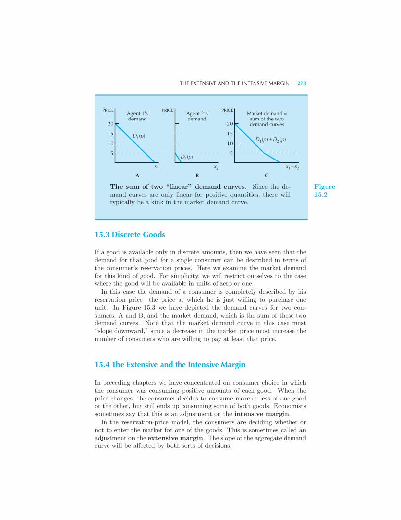
THE EXTENSIVE AND THE INTENSIVE MARGIN 273
Market demand =sum of the twodemand curves
Agent 1'sdemand
Agent 2'sdemand
PRICEPRICE PRICE
20
15
10
5
x x21 x1 2x+
CBA
20
15
10
5
D (p)1
D (p)2
D (p)1 D (p)+ 2
The sum of two “linear” demand curves. Since the de-mand curves are only linear for positive quantities, there willtypically be a kink in the market demand curve.
Figure15.2
15.3 Discrete Goods
If a good is available only in discrete amounts, then we have seen that thedemand for that good for a single consumer can be described in terms ofthe consumer’s reservation prices. Here we examine the market demandfor this kind of good. For simplicity, we will restrict ourselves to the casewhere the good will be available in units of zero or one.In this case the demand of a consumer is completely described by his
reservation price—the price at which he is just willing to purchase oneunit. In Figure 15.3 we have depicted the demand curves for two con-sumers, A and B, and the market demand, which is the sum of these twodemand curves. Note that the market demand curve in this case must“slope downward,” since a decrease in the market price must increase thenumber of consumers who are willing to pay at least that price.
15.4 The Extensive and the Intensive Margin
In preceding chapters we have concentrated on consumer choice in whichthe consumer was consuming positive amounts of each good. When theprice changes, the consumer decides to consume more or less of one goodor the other, but still ends up consuming some of both goods. Economistssometimes say that this is an adjustment on the intensive margin.
In the reservation-price model, the consumers are deciding whether ornot to enter the market for one of the goods. This is sometimes called anadjustment on the extensive margin. The slope of the aggregate demandcurve will be affected by both sorts of decisions.
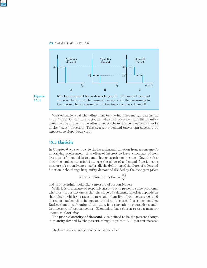
274 MARKET DEMAND (Ch. 15)
.......... .....
.....p*
B
A
A B
B
A
p* p*
p*
x x x + x
A B C
Agent A'sdemand
Agent B'sdemand
Demandmarket
A B
Figure15.3
Market demand for a discrete good. The market demandcurve is the sum of the demand curves of all the consumers inthe market, here represented by the two consumers A and B.
We saw earlier that the adjustment on the intensive margin was in the“right” direction for normal goods: when the price went up, the quantitydemanded went down. The adjustment on the extensive margin also worksin the “right” direction. Thus aggregate demand curves can generally beexpected to slope downward.
15.5 Elasticity
In Chapter 6 we saw how to derive a demand function from a consumer’sunderlying preferences. It is often of interest to have a measure of how“responsive” demand is to some change in price or income. Now the firstidea that springs to mind is to use the slope of a demand function as ameasure of responsiveness. After all, the definition of the slope of a demandfunction is the change in quantity demanded divided by the change in price:
slope of demand function =Δq
Δp,
and that certainly looks like a measure of responsiveness.Well, it is a measure of responsiveness—but it presents some problems.
The most important one is that the slope of a demand function depends onthe units in which you measure price and quantity. If you measure demandin gallons rather than in quarts, the slope becomes four times smaller.Rather than specify units all the time, it is convenient to consider a unit-free measure of responsiveness. Economists have chosen to use a measureknown as elasticity.
The price elasticity of demand, ε, is defined to be the percent changein quantity divided by the percent change in price.1 A 10 percent increase
1 The Greek letter ε, epsilon, is pronounced “eps-i-lon.”
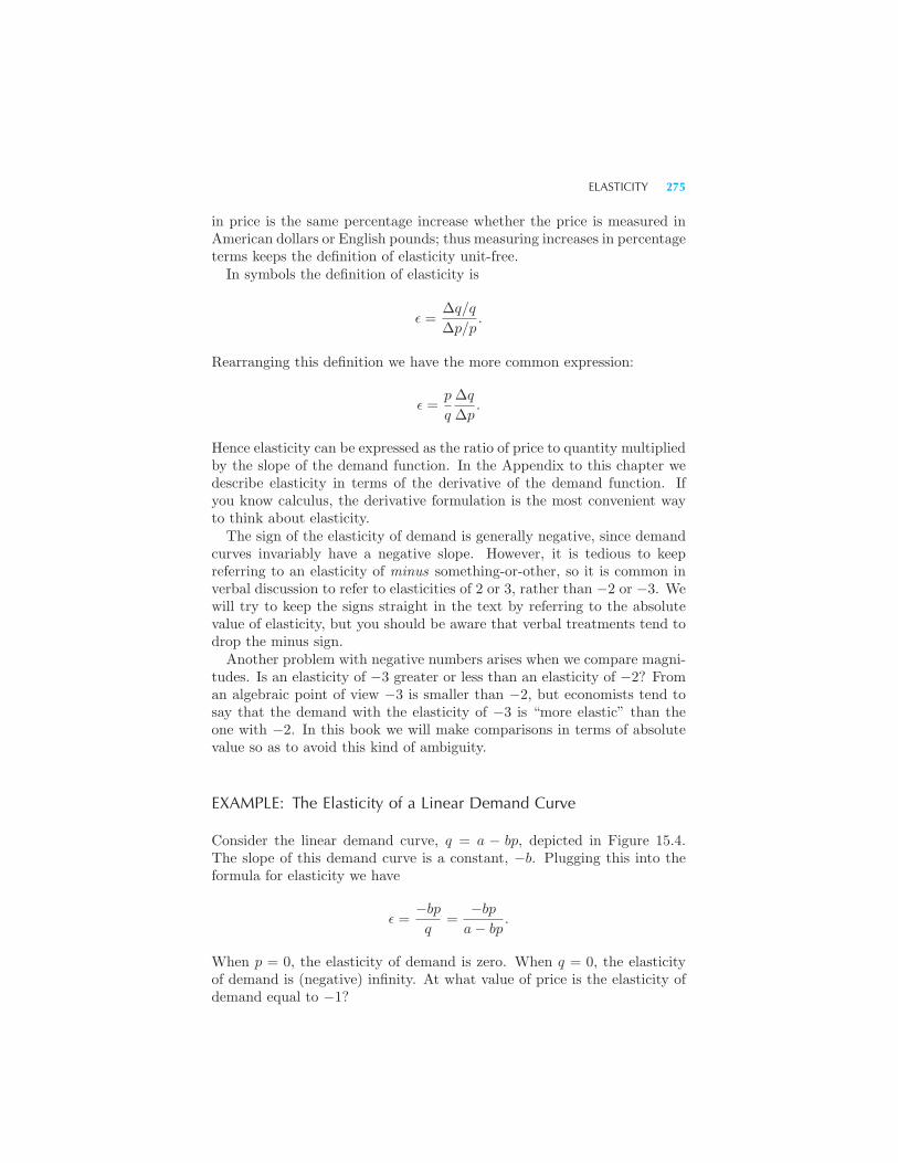
ELASTICITY 275
in price is the same percentage increase whether the price is measured inAmerican dollars or English pounds; thus measuring increases in percentageterms keeps the definition of elasticity unit-free.In symbols the definition of elasticity is
ε =Δq/q
Δp/p.
Rearranging this definition we have the more common expression:
ε =p
q
Δq
Δp.
Hence elasticity can be expressed as the ratio of price to quantity multipliedby the slope of the demand function. In the Appendix to this chapter wedescribe elasticity in terms of the derivative of the demand function. Ifyou know calculus, the derivative formulation is the most convenient wayto think about elasticity.The sign of the elasticity of demand is generally negative, since demand
curves invariably have a negative slope. However, it is tedious to keepreferring to an elasticity of minus something-or-other, so it is common inverbal discussion to refer to elasticities of 2 or 3, rather than −2 or −3. Wewill try to keep the signs straight in the text by referring to the absolutevalue of elasticity, but you should be aware that verbal treatments tend todrop the minus sign.Another problem with negative numbers arises when we compare magni-
tudes. Is an elasticity of −3 greater or less than an elasticity of −2? Froman algebraic point of view −3 is smaller than −2, but economists tend tosay that the demand with the elasticity of −3 is “more elastic” than theone with −2. In this book we will make comparisons in terms of absolutevalue so as to avoid this kind of ambiguity.
EXAMPLE: The Elasticity of a Linear Demand Curve
Consider the linear demand curve, q = a − bp, depicted in Figure 15.4.The slope of this demand curve is a constant, −b. Plugging this into theformula for elasticity we have
ε =−bp
q=
−bp
a− bp.
When p = 0, the elasticity of demand is zero. When q = 0, the elasticityof demand is (negative) infinity. At what value of price is the elasticity ofdemand equal to −1?
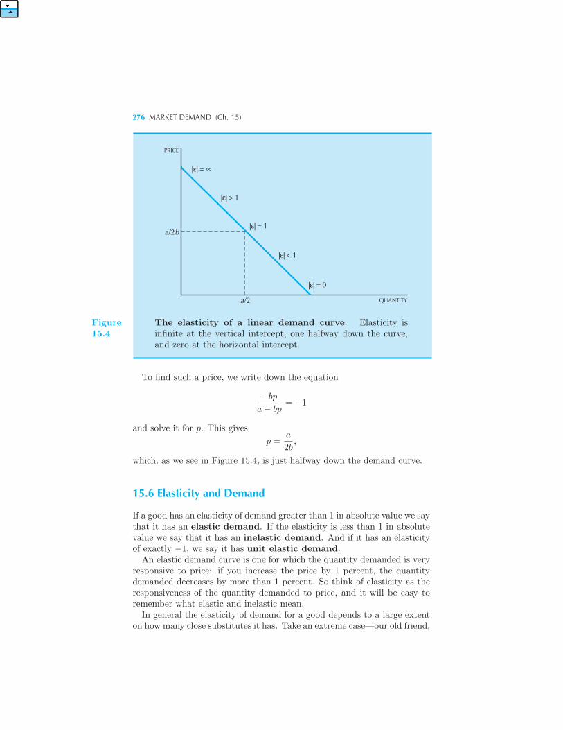
276 MARKET DEMAND (Ch. 15)
|ε| =
|ε| = 0
|ε| = 1
|ε| > 1
|ε| < 1
PRICE
a/2b
a/2 QUANTITY
∞
Figure15.4
The elasticity of a linear demand curve. Elasticity isinfinite at the vertical intercept, one halfway down the curve,and zero at the horizontal intercept.
To find such a price, we write down the equation
−bp
a− bp= −1
and solve it for p. This gives
p =a
2b,
which, as we see in Figure 15.4, is just halfway down the demand curve.
15.6 Elasticity and Demand
If a good has an elasticity of demand greater than 1 in absolute value we saythat it has an elastic demand. If the elasticity is less than 1 in absolutevalue we say that it has an inelastic demand. And if it has an elasticityof exactly −1, we say it has unit elastic demand.An elastic demand curve is one for which the quantity demanded is very
responsive to price: if you increase the price by 1 percent, the quantitydemanded decreases by more than 1 percent. So think of elasticity as theresponsiveness of the quantity demanded to price, and it will be easy toremember what elastic and inelastic mean.In general the elasticity of demand for a good depends to a large extent
on how many close substitutes it has. Take an extreme case—our old friend,
ELASTICITY AND REVENUE 277
the red pencils and blue pencils example. Suppose that everyone regardsthese goods as perfect substitutes. Then if some of each of them are bought,they must sell for the same price. Now think what would happen to thedemand for red pencils if their price rose, and the price of blue pencilsstayed constant. Clearly it would drop to zero—the demand for red pencilsis very elastic since it has a perfect substitute.If a good has many close substitutes, we would expect that its demand
curve would be very responsive to its price changes. On the other hand, ifthere are few close substitutes for a good, it can exhibit a quite inelasticdemand.
15.7 Elasticity and Revenue
Revenue is just the price of a good times the quantity sold of that good.If the price of a good increases, then the quantity sold decreases, so revenuemay increase or decrease. Which way it goes obviously depends on howresponsive demand is to the price change. If demand drops a lot when theprice increases, then revenue will fall. If demand drops only a little when theprice increases, then revenue will increase. This suggests that the directionof the change in revenue has something to do with the elasticity of demand.Indeed, there is a very useful relationship between price elasticity and
revenue change. The definition of revenue is
R = pq.
If we let the price change to p+Δp and the quantity change to q+Δq, wehave a new revenue of
R′ = (p+Δp)(q +Δq)
= pq + qΔp+ pΔq +ΔpΔq.
Subtracting R from R′ we have
ΔR = qΔp+ pΔq +ΔpΔq.
For small values of Δp and Δq, the last term can safely be neglected, leavingus with an expression for the change in revenue of the form
ΔR = qΔp+ pΔq.
That is, the change in revenue is roughly equal to the quantity times thechange in price plus the original price times the change in quantity. If wewant an expression for the rate of change of revenue per change in price,we just divide this expression by Δp to get
ΔR
Δp= q + p
Δq
Δp.
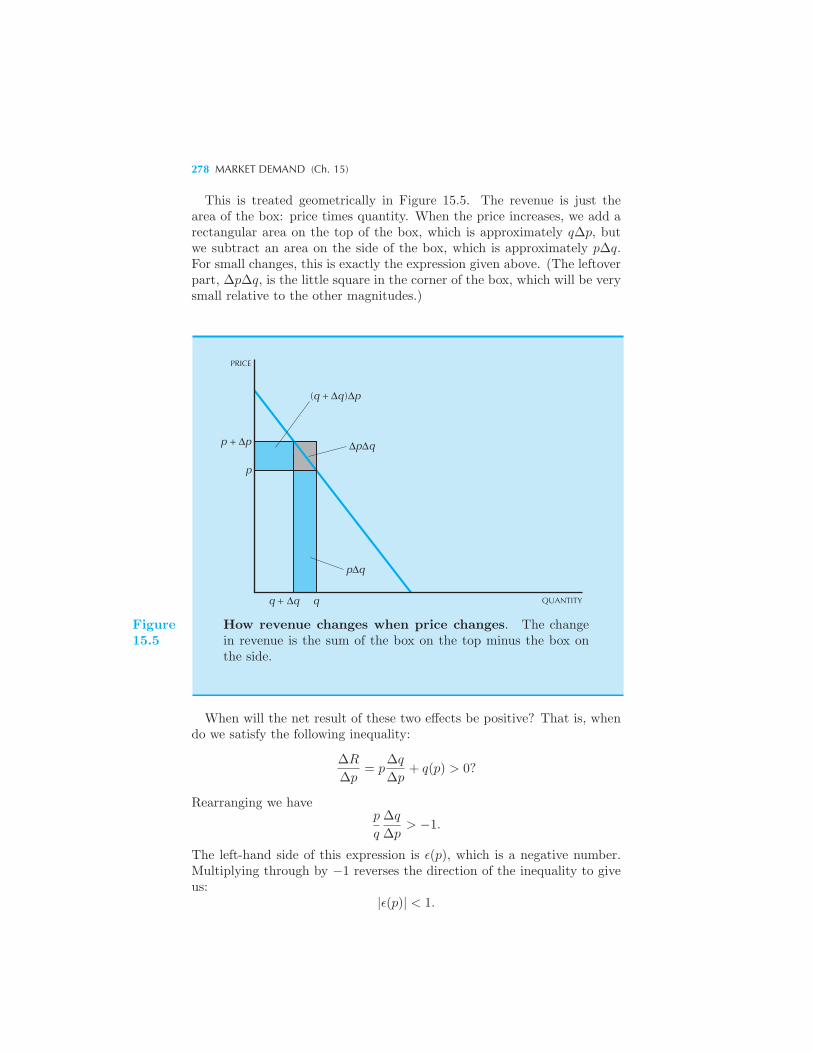
278 MARKET DEMAND (Ch. 15)
This is treated geometrically in Figure 15.5. The revenue is just thearea of the box: price times quantity. When the price increases, we add arectangular area on the top of the box, which is approximately qΔp, butwe subtract an area on the side of the box, which is approximately pΔq.For small changes, this is exactly the expression given above. (The leftoverpart, ΔpΔq, is the little square in the corner of the box, which will be verysmall relative to the other magnitudes.)
ΔpΔq
pΔq
q + Δq q
p + Δp
QUANTITY
p
PRICE
(q + q )Δ Δp
Figure15.5
How revenue changes when price changes. The changein revenue is the sum of the box on the top minus the box onthe side.
When will the net result of these two effects be positive? That is, whendo we satisfy the following inequality:
ΔR
Δp= p
Δq
Δp+ q(p) > 0?
Rearranging we havep
q
Δq
Δp> −1.
The left-hand side of this expression is ε(p), which is a negative number.Multiplying through by −1 reverses the direction of the inequality to giveus:
|ε(p)| < 1.
ELASTICITY AND REVENUE 279
Thus revenue increases when price increases if the elasticity of demandis less than 1 in absolute value. Similarly, revenue decreases when priceincreases if the elasticity of demand is greater than 1 in absolute value.
Another way to see this is to write the revenue change as we did above:
ΔR = pΔq + qΔp > 0
and rearrange this to get
−p
q
Δq
Δp= |ε(p)| < 1.
Yet a third way to see this is to take the formula for ΔR/Δp and rear-range it as follows:
ΔR
Δp= q + p
Δq
Δp
= q
[1 +
p
q
Δq
Δp
]
= q [1 + ε(p)] .
Since demand elasticity is naturally negative, we can also write this ex-pression as
ΔR
Δp= q [1− |ε(p)|] .
In this formula it is easy to see how revenue responds to a change in price:if the absolute value of elasticity is greater than 1, then ΔR/Δp must benegative and vice versa.
The intuitive content of these mathematical facts is not hard to remem-ber. If demand is very responsive to price—that is, it is very elastic—thenan increase in price will reduce demand so much that revenue will fall.If demand is very unresponsive to price—it is very inelastic—then an in-crease in price will not change demand very much, and overall revenue willincrease. The dividing line happens to be an elasticity of −1. At this pointif the price increases by 1 percent, the quantity will decrease by 1 percent,so overall revenue doesn’t change at all.
EXAMPLE: Strikes and Profits
In 1979 the United Farm Workers called for a strike against lettuce growersin California. The strike was highly effective: the production of lettuce wascut almost in half. But the reduction in the supply of lettuce inevitablycaused an increase in the price of lettuce. In fact, during the strike the price
280 MARKET DEMAND (Ch. 15)
of lettuce rose by nearly 400 percent. Since production halved and pricesquadrupled, the net result of was almost a doubling producer profits!2
One might well ask why the producers eventually settled the strike. Theanswer involves short-run and long-run supply responses. Most of the let-tuce consumed in U.S. during the winter months is grown in the ImperialValley. When the supply of this lettuce was drastically reduced in oneseason, there wasn’t time to replace it with lettuce from elsewhere so themarket price of lettuce skyrocketed. If the strike had held for several sea-sons, lettuce could be planted in other regions. This increase in supply fromother sources would tend reduce the price of lettuce back to its normal level,thereby reducing the profits of the Imperial Valley growers.
15.8 Constant Elasticity Demands
What kind of demand curve gives us a constant elasticity of demand? Ina linear demand curve the elasticity of demand goes from zero to infinity,which is not exactly what you would call constant, so that’s not the answer.We can use the revenue calculation described above to get an example.
We know that if the elasticity is 1 at price p, then the revenue will notchange when the price changes by a small amount. So if the revenue remainsconstant for all changes in price, we must have a demand curve that hasan elasticity of −1 everywhere.But this is easy. We just want price and quantity to be related by the
formulapq = R,
which means that
q =R
p
is the formula for a demand function with constant elasticity of −1. Thegraph of the function q = R/p is given in Figure 15.6. Note that pricetimes quantity is constant along the demand curve.The general formula for a demand with a constant elasticity of ε turns
out to beq = Apε,
where A is an arbitrary positive constant and ε, being an elasticity, willtypically be negative. This formula will be useful in some examples lateron.A convenient way to express a constant elasticity demand curve is to
take logarithms and write
ln q = lnA+ ε ln p.
2 See Colin Carter, et. al., “Agricultural Labor Strikes and Farmers’ Incomes,” Eco-nomic Inquiry, 25, 1987,121–133.
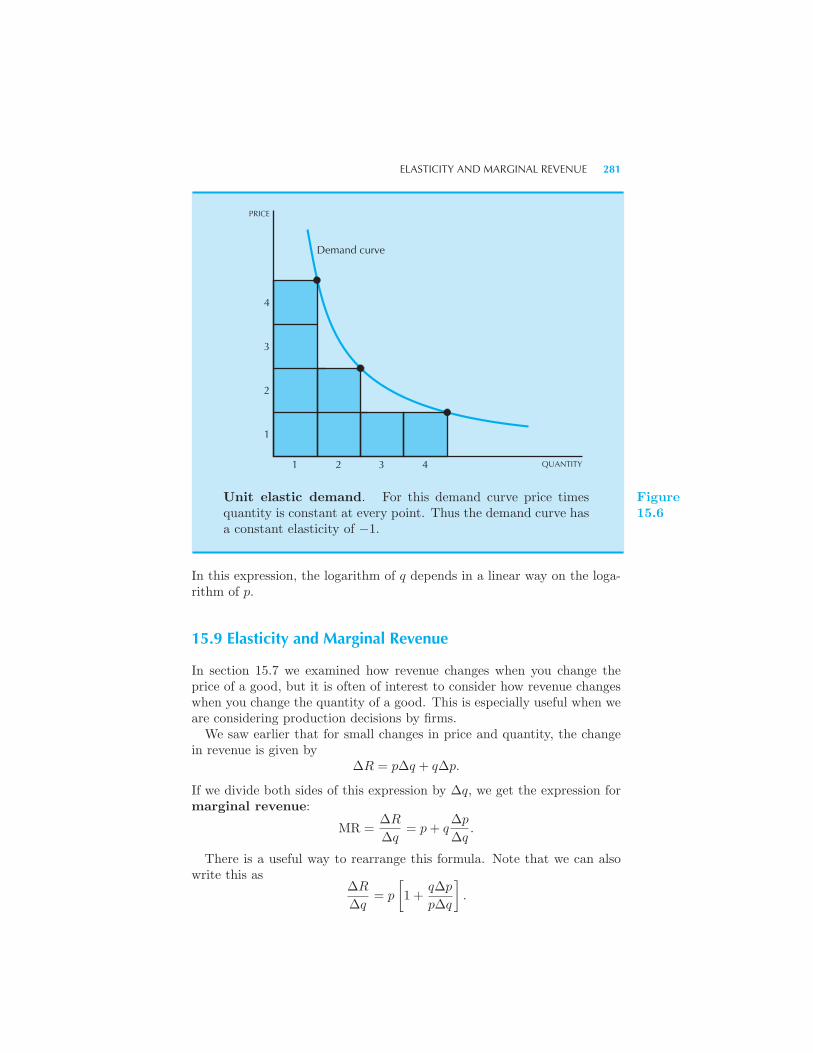
ELASTICITY AND MARGINAL REVENUE 281
Demand curve
PRICE
QUANTITY1 2 3 4
4
3
2
1
Unit elastic demand. For this demand curve price timesquantity is constant at every point. Thus the demand curve hasa constant elasticity of −1.
Figure15.6
In this expression, the logarithm of q depends in a linear way on the loga-rithm of p.
15.9 Elasticity and Marginal Revenue
In section 15.7 we examined how revenue changes when you change theprice of a good, but it is often of interest to consider how revenue changeswhen you change the quantity of a good. This is especially useful when weare considering production decisions by firms.We saw earlier that for small changes in price and quantity, the change
in revenue is given byΔR = pΔq + qΔp.
If we divide both sides of this expression by Δq, we get the expression formarginal revenue:
MR =ΔR
Δq= p+ q
Δp
Δq.
There is a useful way to rearrange this formula. Note that we can alsowrite this as
ΔR
Δq= p
[1 +
qΔp
pΔq
].
282 MARKET DEMAND (Ch. 15)
What is the second term inside the brackets? Nope, it’s not elasticity, butyou’re close. It is the reciprocal of elasticity:
1
ε=
1pΔqqΔp
=qΔp
pΔq.
Thus the expression for marginal revenue becomes
ΔR
Δq= p(q)
[1 +
1
ε(q)
].
(Here we’ve written p(q) and ε(q) to remind ourselves that both price andelasticity will typically depend on the level of output.)When there is a danger of confusion due to the fact that elasticity is a
negative number we will sometimes write this expression as
ΔR
Δq= p(q)
[1− 1
|ε(q)|
].
This means that if elasticity of demand is −1, then marginal revenueis zero—revenue doesn’t change when you increase output. If demand isinelastic, then |ε| is less than 1, which means 1/|ε| is greater than 1. Thus1−1/|ε| is negative, so that revenue will decrease when you increase output.This is quite intuitive. If demand isn’t very responsive to price, then you
have to cut prices a lot to increase output: so revenue goes down. Thisis all completely consistent with the earlier discussion about how revenuechanges as we change price, since an increase in quantity means a decreasein price and vice versa.
EXAMPLE: Setting a Price
Suppose that you were in charge of setting a price for some product thatyou were producing and that you had a good estimate of the demand curvefor that product. Let us suppose that your goal is to set a price thatmaximizes profits—revenue minus costs. Then you would never want toset it where the elasticity of demand was less than 1—you would neverwant to set a price where demand was inelastic.Why? Consider what would happen if you raised your price. Then your
revenues would increase—since demand was inelastic—and the quantityyou were selling would decrease. But if the quantity sold decreases, thenyour production costs must also decrease, or at least, they can’t increase.So your overall profit must rise, which shows that operating at an inelasticpart of the demand curve cannot yield maximal profits.
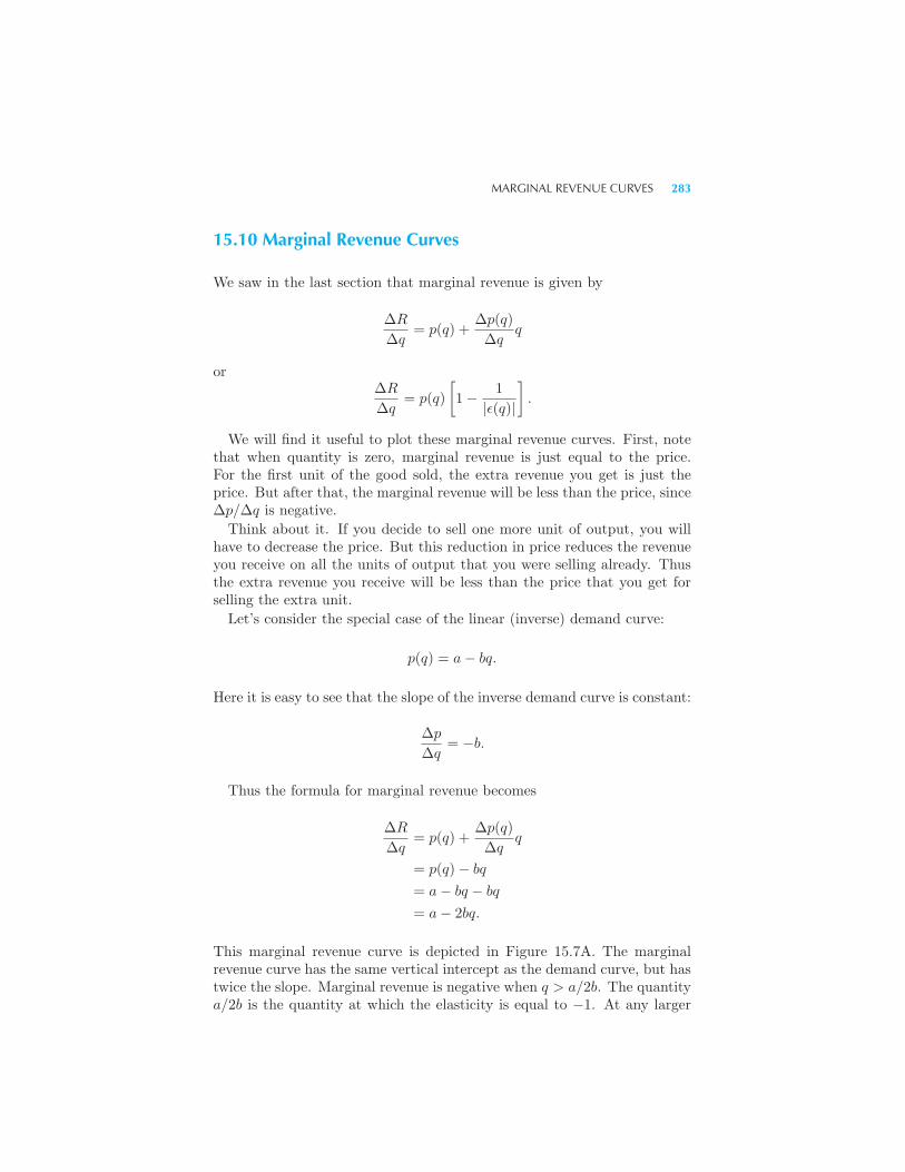
MARGINAL REVENUE CURVES 283
15.10 Marginal Revenue Curves
We saw in the last section that marginal revenue is given by
ΔR
Δq= p(q) +
Δp(q)
Δqq
orΔR
Δq= p(q)
[1− 1
|ε(q)|
].
We will find it useful to plot these marginal revenue curves. First, notethat when quantity is zero, marginal revenue is just equal to the price.For the first unit of the good sold, the extra revenue you get is just theprice. But after that, the marginal revenue will be less than the price, sinceΔp/Δq is negative.
Think about it. If you decide to sell one more unit of output, you willhave to decrease the price. But this reduction in price reduces the revenueyou receive on all the units of output that you were selling already. Thusthe extra revenue you receive will be less than the price that you get forselling the extra unit.
Let’s consider the special case of the linear (inverse) demand curve:
p(q) = a− bq.
Here it is easy to see that the slope of the inverse demand curve is constant:
Δp
Δq= −b.
Thus the formula for marginal revenue becomes
ΔR
Δq= p(q) +
Δp(q)
Δqq
= p(q)− bq
= a− bq − bq
= a− 2bq.
This marginal revenue curve is depicted in Figure 15.7A. The marginalrevenue curve has the same vertical intercept as the demand curve, but hastwice the slope. Marginal revenue is negative when q > a/2b. The quantitya/2b is the quantity at which the elasticity is equal to −1. At any larger
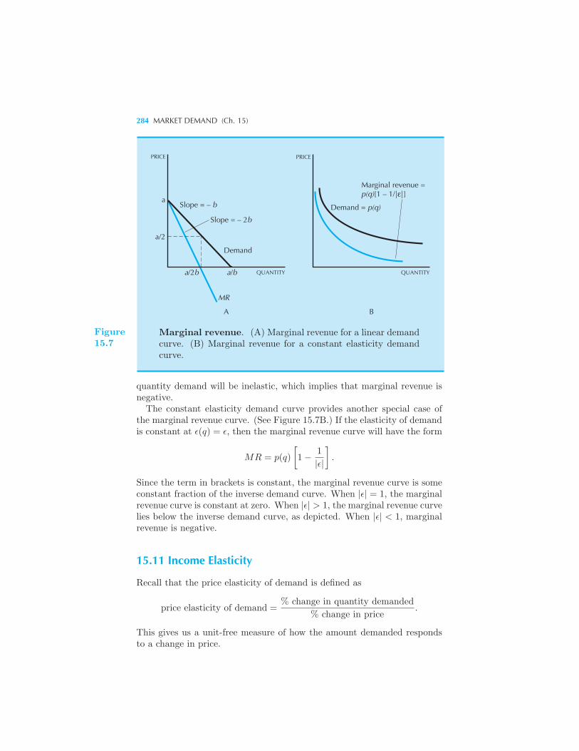
284 MARKET DEMAND (Ch. 15)
Demand = p(q)
Marginal revenue =p(q)[1 – 1/|ε|]
QUANTITY
PRICEPRICE
QUANTITY
MR
a
a/2
Demand
Slope = – 2b
Slope = – b
a/ba/2b
A B
Figure15.7
Marginal revenue. (A) Marginal revenue for a linear demandcurve. (B) Marginal revenue for a constant elasticity demandcurve.
quantity demand will be inelastic, which implies that marginal revenue isnegative.The constant elasticity demand curve provides another special case of
the marginal revenue curve. (See Figure 15.7B.) If the elasticity of demandis constant at ε(q) = ε, then the marginal revenue curve will have the form
MR = p(q)
[1− 1
|ε|
].
Since the term in brackets is constant, the marginal revenue curve is someconstant fraction of the inverse demand curve. When |ε| = 1, the marginalrevenue curve is constant at zero. When |ε| > 1, the marginal revenue curvelies below the inverse demand curve, as depicted. When |ε| < 1, marginalrevenue is negative.
15.11 Income Elasticity
Recall that the price elasticity of demand is defined as
price elasticity of demand =% change in quantity demanded
% change in price.
This gives us a unit-free measure of how the amount demanded respondsto a change in price.
SUMMARY 285
The income elasticity of demand is used to describe how the quantitydemanded responds to a change in income; its definition is
income elasticity of demand =% change in quantity
% change in income.
Recall that a normal good is one for which an increase in income leadsto an increase in demand; so for this sort of good the income elasticityof demand is positive. An inferior good is one for which an increase inincome leads to a decrease in demand; for this sort of good, the incomeelasticity of demand is negative. Economists sometimes use the term lux-ury goods. These are goods that have an income elasticity of demandthat is greater than 1: a 1 percent increase in income leads to more thana 1 percent increase in demand for a luxury good.As a general rule of thumb, however, income elasticities tend to clus-
ter around 1. We can see the reason for this by examining the budgetconstraint. Write the budget constraints for two different levels of income:
p1x′1 + p2x
′2 = m′
p1x01 + p2x
02 = m0.
Subtract the second equation from the first and let Δ denote differences,as usual:
p1 Δx1 + p2 Δx2 = Δm.
Now multiply and divide price i by xi/xi and divide both sides by m:
p1x1
m
Δx1
x1+
p2x2
m
Δx2
x2=
Δm
m.
Finally, divide both sides by Δm/m, and use si = pixi/m to denote theexpenditure share of good i. This gives us our final equation,
s1Δx1/x1
Δm/m+ s2
Δx2/x2
Δm/m= 1.
This equation says that the weighted average of the income elasticities is1, where the weights are the expenditure shares. Luxury goods that havean income elasticity greater than 1 must be counterbalanced by goods thathave an income elasticity less than 1, so that “on average” income elastic-ities are about 1.
Summary
1. The market demand curve is simply the sum of the individual demandcurves.
286 MARKET DEMAND (Ch. 15)
2. The reservation price measures the price at which a consumer is justindifferent between purchasing or not purchasing a good.
3. The demand function measures quantity demanded as a function ofprice. The inverse demand function measures price as a function of quan-tity. A given demand curve can be described in either way.
4. The elasticity of demand measures the responsiveness of the quantitydemanded to price. It is formally defined as the percent change in quantitydivided by the percent change in price.
5. If the absolute value of the elasticity of demand is less than 1 at somepoint, we say that demand is inelastic at that point. If the absolute valueof elasticity is greater than 1 at some point, we say demand is elastic atthat point. If the absolute value of the elasticity of demand at some pointis exactly 1, we say that the demand has unitary elasticity at that point.
6. If demand is inelastic at some point, then an increase in quantity willresult in a reduction in revenue. If demand is elastic, then an increase inquantity will result in an increase in revenue.
7. The marginal revenue is the extra revenue one gets from increasingthe quantity sold. The formula relating marginal revenue and elasticityis MR = p[1 + 1/ε] = p[1− 1/|ε|].
8. If the inverse demand curve is a linear function p(q) = a− bq, then themarginal revenue is given by MR = a− 2bq.
9. Income elasticity measures the responsiveness of the quantity demandedto income. It is formally defined as the percent change in quantity dividedby the percent change in income.
REVIEW QUESTIONS
1. If the market demand curve is D(p) = 100 − .5p, what is the inversedemand curve?
2. An addict’s demand function for a drug may be very inelastic, but themarket demand function might be quite elastic. How can this be?
3. If D(p) = 12− 2p, what price will maximize revenue?
4. Suppose that the demand curve for a good is given by D(p) = 100/p.What price will maximize revenue?
5. True or false? In a two good model if one good is an inferior good theother good must be a luxury good.
APPENDIX 287
APPENDIX
In terms of derivatives the price elasticity of demand is defined by
ε =p
q
dq
dp.
In the text we claimed that the formula for a constant elasticity demand curvewas q = Apε. To verify that this is correct, we can just differentiate it withrespect to price:
dq
dp= εApε−1
and multiply by price over quantity:
p
q
dq
dp=
p
ApεεApε−1 = ε.
Everything conveniently cancels, leaving us with ε as required.
A linear demand curve has the formula q(p) = a−bp. The elasticity of demandat a point p is given by
ε =p
q
dq
dp=
−bp
a− bp.
When p is zero, the elasticity is zero. When q is zero, the elasticity is infinite.
Revenue is given by R(p) = pq(p). To see how revenue changes as p changeswe differentiate revenue with respect to p to get
R′(p) = pq′(p) + q(p).
Suppose that revenue increases when p increases. Then we have
R′(p) = pdq
dp+ q(p) > 0.
Rearranging, we have
ε =p
q
dq
dp> −1.
Recalling that dq/dp is negative and multiplying through by −1, we find
|ε| < 1.
Hence if revenue increases when price increases, we must be at an inelastic partof the demand curve.
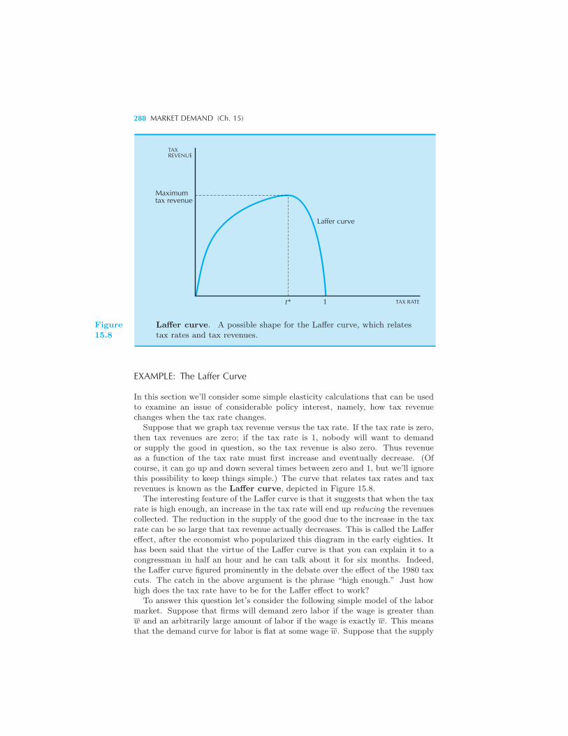
288 MARKET DEMAND (Ch. 15)
TAXREVENUE
Maximumtax revenue
Laffer curve
1t* TAX RATE
Figure15.8
Laffer curve. A possible shape for the Laffer curve, which relatestax rates and tax revenues.
EXAMPLE: The Laffer Curve
In this section we’ll consider some simple elasticity calculations that can be usedto examine an issue of considerable policy interest, namely, how tax revenuechanges when the tax rate changes.
Suppose that we graph tax revenue versus the tax rate. If the tax rate is zero,then tax revenues are zero; if the tax rate is 1, nobody will want to demandor supply the good in question, so the tax revenue is also zero. Thus revenueas a function of the tax rate must first increase and eventually decrease. (Ofcourse, it can go up and down several times between zero and 1, but we’ll ignorethis possibility to keep things simple.) The curve that relates tax rates and taxrevenues is known as the Laffer curve, depicted in Figure 15.8.
The interesting feature of the Laffer curve is that it suggests that when the taxrate is high enough, an increase in the tax rate will end up reducing the revenuescollected. The reduction in the supply of the good due to the increase in the taxrate can be so large that tax revenue actually decreases. This is called the Laffereffect, after the economist who popularized this diagram in the early eighties. Ithas been said that the virtue of the Laffer curve is that you can explain it to acongressman in half an hour and he can talk about it for six months. Indeed,the Laffer curve figured prominently in the debate over the effect of the 1980 taxcuts. The catch in the above argument is the phrase “high enough.” Just howhigh does the tax rate have to be for the Laffer effect to work?
To answer this question let’s consider the following simple model of the labormarket. Suppose that firms will demand zero labor if the wage is greater thanw and an arbitrarily large amount of labor if the wage is exactly w. This meansthat the demand curve for labor is flat at some wage w. Suppose that the supply
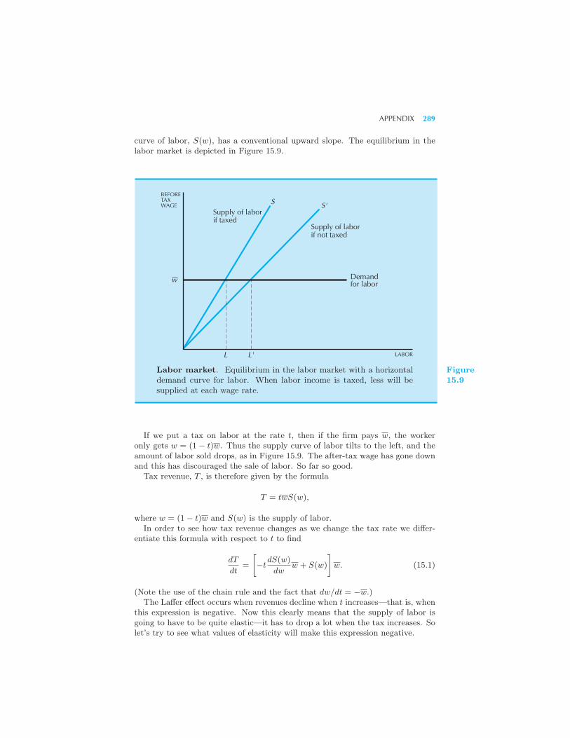
APPENDIX 289
curve of labor, S(w), has a conventional upward slope. The equilibrium in thelabor market is depicted in Figure 15.9.
Demandfor labor
Supply of laborif not taxed
Supply of laborif taxed
S S'
w
L L' LABOR
BEFORETAXWAGE
Labor market. Equilibrium in the labor market with a horizontaldemand curve for labor. When labor income is taxed, less will besupplied at each wage rate.
Figure15.9
If we put a tax on labor at the rate t, then if the firm pays w, the workeronly gets w = (1− t)w. Thus the supply curve of labor tilts to the left, and theamount of labor sold drops, as in Figure 15.9. The after-tax wage has gone downand this has discouraged the sale of labor. So far so good.
Tax revenue, T , is therefore given by the formula
T = twS(w),
where w = (1− t)w and S(w) is the supply of labor.In order to see how tax revenue changes as we change the tax rate we differ-
entiate this formula with respect to t to find
dT
dt=
[−t
dS(w)
dww + S(w)
]w. (15.1)
(Note the use of the chain rule and the fact that dw/dt = −w.)The Laffer effect occurs when revenues decline when t increases—that is, when
this expression is negative. Now this clearly means that the supply of labor isgoing to have to be quite elastic—it has to drop a lot when the tax increases. Solet’s try to see what values of elasticity will make this expression negative.
290 MARKET DEMAND (Ch. 15)
In order for equation (15.1) to be negative, we must have
−tdS(w)
dww + S(w) < 0.
Transposing yields
tdS(w)
dww > S(w),
and dividing both sides by tS(w) gives
dS(w)
dw
w
S(w)>
1
t.
Multiplying both sides by (1− t) and using the fact that w = (1− t)w gives us
dS
dw
w
S>
1− t
t.
The left-hand side of this expression is the elasticity of labor supply. We haveshown that the Laffer effect can only occur if the elasticity of labor supply isgreater than (1− t)/t.
Let us take an extreme case and suppose that the tax rate on labor incomeis 50 percent. Then the Laffer effect can occur only when the elasticity of laborsupply is greater than 1. This means that a 1 percent reduction in the wagewould lead to more than a 1 percent reduction in the labor supply. This is a verylarge response.
Econometricians have often estimated labor-supply elasticities, and about thelargest value anyone has ever found has been around 0.2. So the Laffer effectseems pretty unlikely for the kinds of tax rates that we have in the United States.However, in other countries, such as Sweden, tax rates go much higher, and thereis some evidence that the Laffer phenomenon may have occurred.3
EXAMPLE: Another Expression for Elasticity
Here is another expression for elasticity that is sometimes useful. It turns outthat elasticity can also be expressed as
d lnQ
d lnP.
The proof involves repeated application of the chain rule. We start by notingthat
d lnQ
d lnP=
d lnQ
dQ
dQ
d lnP
=1
Q
dQ
d lnP. (15.2)
3 See Charles E. Stuart, “Swedish Tax Rates, Labor Supply, and Tax Revenues,” Jour-nal of Political Economy, 89, 5 (October 1981), 1020–38.
APPENDIX 291
We also note thatdQ
dP=
dQ
d lnP
d lnP
dP
=dQ
d lnP
1
P,
which implies thatdQ
d lnP= P
dQ
dP.
Substituting this into equation (15.2), we have
d lnQ
d lnP=
1
Q
dQ
dPP = ε,
which is what we wanted to establish.Thus elasticity measures the slope of the demand curve plotted on log-log
paper: how the log of the quantity changes as the log of the price changes.
CHAPTER 16
EQUILIBRIUM
In preceding chapters we have seen how to construct individual demandcurves by using information about preferences and prices. In Chapter 15we added up these individual demand curves to construct market demandcurves. In this chapter we will describe how to use these market demandcurves to determine the equilibrium market price.In Chapter 1 we said that there were two fundamental principles of micro-
economic analysis. These were the optimization principle and the equilib-rium principle. Up until now we have been studying examples of the opti-mization principle: what follows from the assumption that people choosetheir consumption optimally from their budget sets. In later chapters wewill continue to use optimization analysis to study the profit-maximizationbehavior of firms. Finally, we combine the behavior of consumers and firmsto study the equilibrium outcomes of their interaction in the market.But before undertaking that study in detail it seems worthwhile at this
point to give some examples of equilibrium analysis—how the prices adjustso as to make the demand and supply decisions of economic agents com-patible. In order to do so, we will have to briefly consider the other side ofthe market—the supply side.
MARKET EQUILIBRIUM 293
16.1 Supply
We have already seen a few examples of supply curves. In Chapter 1we looked at a vertical supply curve for apartments. In Chapter 9 weconsidered situations where consumers would choose to be net suppliersor demanders of goods that they owned, and we analyzed labor-supplydecisions.In all of these cases the supply curve simply measured how much the
consumer was willing to supply of a good at each possible market price.Indeed, this is the definition of the supply curve: for each p, we determinehow much of the good will be supplied, S(p). In the next few chapters wewill discuss the supply behavior of firms. However, for many purposes, it isnot really necessary to know where the supply curve or the demand curvecomes from in terms of the optimizing behavior that generates the curves.For many problems the fact that there is a functional relationship betweenthe price and the quantity that consumers want to demand or supply atthat price is enough to highlight important insights.
16.2 Market Equilibrium
Suppose that we have a number of consumers of a good. Given theirindividual demand curves we can add them up to get a market demandcurve. Similarly, if we have a number of independent suppliers of thisgood, we can add up their individual supply curves to get the marketsupply curve.The individual demanders and suppliers are assumed to take prices as
given—outside of their control—and simply determine their best responsegiven those market prices. A market where each economic agent takesthe market price as outside of his or her control is called a competitivemarket.The usual justification for the competitive-market assumption is that
each consumer or producer is a small part of the market as a whole andthus has a negligible effect on the market price. For example, each supplierof wheat takes the market price to be more or less independent of his actionswhen he determines how much wheat he wants to produce and supply tothe market.Although the market price may be independent of any one agent’s actions
in a competitive market, it is the actions of all the agents together thatdetermine the market price. The equilibrium price of a good is thatprice where the supply of the good equals the demand. Geometrically, thisis the price where the demand and the supply curves cross.If we let D(p) be the market demand curve and S(p) the market supply
curve, the equilibrium price is the price p∗ that solves the equation
D(p∗) = S(p∗).
294 EQUILIBRIUM (Ch. 16)
The solution to this equation, p∗, is the price where market demand equalsmarket supply.
Why should this be an equilibrium price? An economic equilibriumis a situation where all agents are choosing the best possible action forthemselves and each person’s behavior is consistent with that of the others.At any price other than an equilibrium price, some agents’ behaviors wouldbe infeasible, and there would therefore be a reason for their behavior tochange. Thus a price that is not an equilibrium price cannot be expected topersist since at least some agents would have an incentive to change theirbehavior.
The demand and supply curves represent the optimal choices of theagents involved, and the fact that they are equal at some price p∗ indi-cates that the behaviors of the demanders and suppliers are compatible.At any price other than the price where demand equals supply these twoconditions will not be met.
For example, suppose that we consider some price p′ < p∗ where demandis greater than supply. Then some suppliers will realize that they can selltheir goods at more than the going price p′ to the disappointed demanders.As more and more suppliers realize this, the market price will be pushedup to the point where demand and supply are equal.
Similarly if p′ > p∗, so that demand is less than supply, then somesuppliers will not be able to sell the amount that they expected to sell.The only way in which they will be able to sell more output will be to offerit at a lower price. But if all suppliers are selling the identical goods, and ifsome supplier offers to sell at a lower price, the other suppliers must matchthat price. Thus excess supply exerts a downward pressure on the marketprice. Only when the amount that people want to buy at a given priceequals the amount that people want to sell at that price will the market bein equilibrium.
16.3 Two Special Cases
There are two special cases of market equilibrium that are worth mentioningsince they come up fairly often. The first is the case of fixed supply. Herethe amount supplied is some given number and is independent of price;that is, the supply curve is vertical. In this case the equilibrium quantityis determined entirely by the supply conditions and the equilibrium priceis determined entirely by demand conditions.
The opposite case is the case where the supply curve is completely hor-izontal. If an industry has a perfectly horizontal supply curve, it meansthat the industry will supply any amount of a good at a constant price. Inthis situation the equilibrium price is determined by the supply conditions,while the equilibrium quantity is determined by the demand curve.
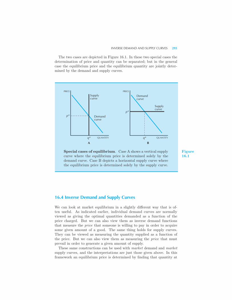
INVERSE DEMAND AND SUPPLY CURVES 295
The two cases are depicted in Figure 16.1. In these two special cases thedetermination of price and quantity can be separated; but in the generalcase the equilibrium price and the equilibrium quantity are jointly deter-mined by the demand and supply curves.
PRICE
Supplycurve
p*
q* QUANTITY
Demandcurve
A
PRICE
Supplycurve
p*
q* QUANTITY
Demandcurve
B
Special cases of equilibrium. Case A shows a vertical supplycurve where the equilibrium price is determined solely by thedemand curve. Case B depicts a horizontal supply curve wherethe equilibrium price is determined solely by the supply curve.
Figure16.1
16.4 Inverse Demand and Supply Curves
We can look at market equilibrium in a slightly different way that is of-ten useful. As indicated earlier, individual demand curves are normallyviewed as giving the optimal quantities demanded as a function of theprice charged. But we can also view them as inverse demand functionsthat measure the price that someone is willing to pay in order to acquiresome given amount of a good. The same thing holds for supply curves.They can be viewed as measuring the quantity supplied as a function ofthe price. But we can also view them as measuring the price that mustprevail in order to generate a given amount of supply.These same constructions can be used with market demand and market
supply curves, and the interpretations are just those given above. In thisframework an equilibrium price is determined by finding that quantity at
296 EQUILIBRIUM (Ch. 16)
which the amount the demanders are willing to pay to consume that quan-tity is the same as the price that suppliers must receive in order to supplythat quantity.Thus, if we let PS(q) be the inverse supply function and PD(q) be the
inverse demand function, equilibrium is determined by the condition
PS(q∗) = PD(q∗).
EXAMPLE: Equilibrium with Linear Curves
Suppose that both the demand and the supply curves are linear:
D(p) = a− bp
S(p) = c+ dp.
The coefficients (a, b, c, d) are the parameters that determine the inter-cepts and slopes of these linear curves. The equilibrium price can be foundby solving the following equation:
D(p) = a− bp = c+ dp = S(p).
The answer is
p∗ =a− c
d+ b.
The equilibrium quantity demanded (and supplied) is
D(p∗) = a− bp∗
= a− ba− c
b+ d
=ad+ bc
b+ d.
We can also solve this problem by using the inverse demand and supplycurves. First we need to find the inverse demand curve. At what price issome quantity q demanded? Simply substitute q for D(p) and solve for p.We have
q = a− bp,
so
PD(q) =a− q
b.
In the same manner we find
PS(q) =q − c
d.
COMPARATIVE STATICS 297
Setting the demand price equal to the supply price and solving for theequilibrium quantity we have
PD(q) =a− q
b=
q − c
d= PS(q)
q∗ =ad+ bc
b+ d.
Note that this gives the same answer as in the original problem for boththe equilibrium price and the equilibrium quantity.
16.5 Comparative Statics
After we have found an equilibrium by using the demand equals supplycondition (or the demand price equals the supply price condition), we cansee how it will change as the demand and supply curves change. For ex-ample, it is easy to see that if the demand curve shifts to the right in aparallel way—some fixed amount more is demanded at every price—theequilibrium price and quantity must both rise. On the other hand, if thesupply curve shifts to the right, the equilibrium quantity rises, but theequilibrium price must fall.What if both curves shift to the right? Then the quantity will definitely
increase while the change in price is ambiguous—it could increase or itcould decrease.
EXAMPLE: Shifting Both Curves
Question: Consider the competitive market for apartments described inChapter 1. Let the equilibrium price in that market be p∗ and the equi-librium quantity be q∗. Suppose that a developer converts m of the apart-ments to condominiums, which are bought by the people who are currentlyliving in the apartments. What happens to the equilibrium price?
Answer: The situation is depicted in Figure 16.2. The demand and sup-ply curves both shift to the left by the same amount. Hence the price isunchanged and the quantity sold simply drops by m.Algebraically the new equilibrium price is determined by
D(p)−m = S(p)−m,
which clearly has the same solution as the original demand equals supplycondition.
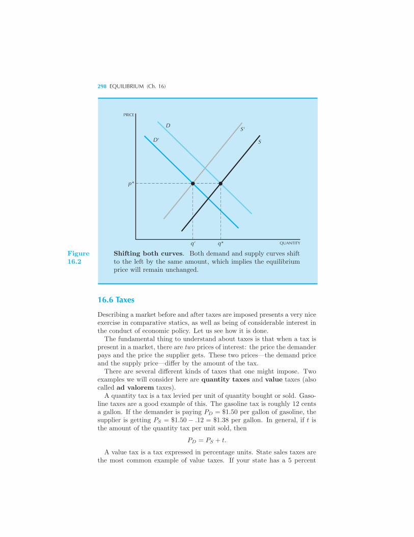
298 EQUILIBRIUM (Ch. 16)
PRICE
D
D'
S'
S
p*
q' q* QUANTITY
Figure16.2
Shifting both curves. Both demand and supply curves shiftto the left by the same amount, which implies the equilibriumprice will remain unchanged.
16.6 Taxes
Describing a market before and after taxes are imposed presents a very niceexercise in comparative statics, as well as being of considerable interest inthe conduct of economic policy. Let us see how it is done.The fundamental thing to understand about taxes is that when a tax is
present in a market, there are two prices of interest: the price the demanderpays and the price the supplier gets. These two prices—the demand priceand the supply price—differ by the amount of the tax.There are several different kinds of taxes that one might impose. Two
examples we will consider here are quantity taxes and value taxes (alsocalled ad valorem taxes).A quantity tax is a tax levied per unit of quantity bought or sold. Gaso-
line taxes are a good example of this. The gasoline tax is roughly 12 centsa gallon. If the demander is paying PD = $1.50 per gallon of gasoline, thesupplier is getting PS = $1.50 − .12 = $1.38 per gallon. In general, if t isthe amount of the quantity tax per unit sold, then
PD = PS + t.
A value tax is a tax expressed in percentage units. State sales taxes arethe most common example of value taxes. If your state has a 5 percent
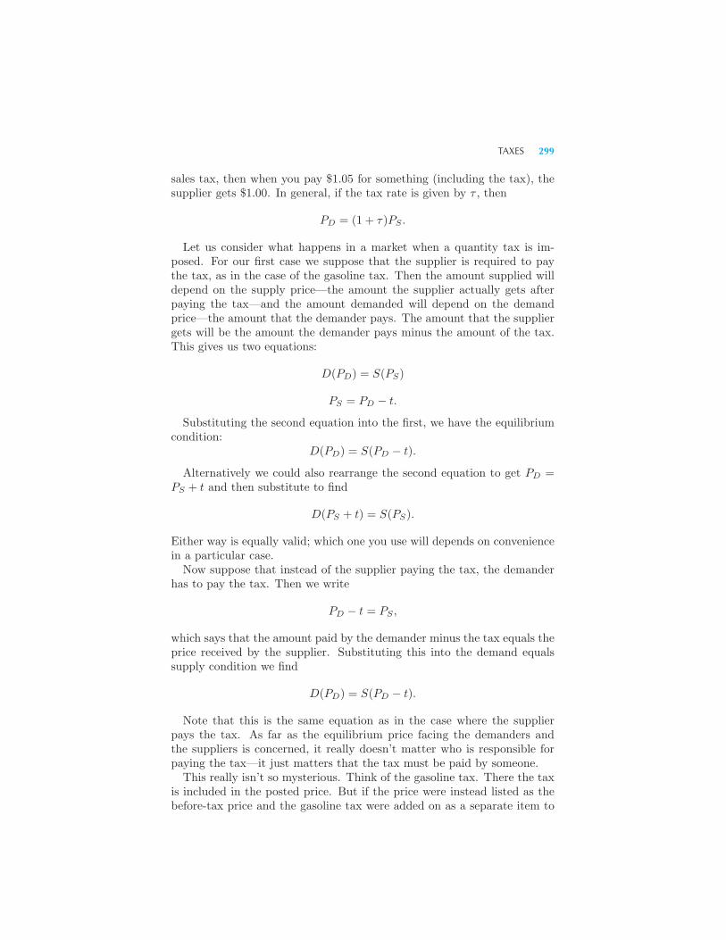
TAXES 299
sales tax, then when you pay $1.05 for something (including the tax), thesupplier gets $1.00. In general, if the tax rate is given by τ , then
PD = (1 + τ)PS .
Let us consider what happens in a market when a quantity tax is im-posed. For our first case we suppose that the supplier is required to paythe tax, as in the case of the gasoline tax. Then the amount supplied willdepend on the supply price—the amount the supplier actually gets afterpaying the tax—and the amount demanded will depend on the demandprice—the amount that the demander pays. The amount that the suppliergets will be the amount the demander pays minus the amount of the tax.This gives us two equations:
D(PD) = S(PS)
PS = PD − t.
Substituting the second equation into the first, we have the equilibriumcondition:
D(PD) = S(PD − t).
Alternatively we could also rearrange the second equation to get PD =PS + t and then substitute to find
D(PS + t) = S(PS).
Either way is equally valid; which one you use will depends on conveniencein a particular case.Now suppose that instead of the supplier paying the tax, the demander
has to pay the tax. Then we write
PD − t = PS ,
which says that the amount paid by the demander minus the tax equals theprice received by the supplier. Substituting this into the demand equalssupply condition we find
D(PD) = S(PD − t).
Note that this is the same equation as in the case where the supplierpays the tax. As far as the equilibrium price facing the demanders andthe suppliers is concerned, it really doesn’t matter who is responsible forpaying the tax—it just matters that the tax must be paid by someone.This really isn’t so mysterious. Think of the gasoline tax. There the tax
is included in the posted price. But if the price were instead listed as thebefore-tax price and the gasoline tax were added on as a separate item to
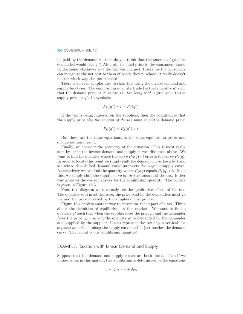
300 EQUILIBRIUM (Ch. 16)
be paid by the demanders, then do you think that the amount of gasolinedemanded would change? After all, the final price to the consumers wouldbe the same whichever way the tax was charged. Insofar as the consumerscan recognize the net cost to them of goods they purchase, it really doesn’tmatter which way the tax is levied.There is an even simpler way to show this using the inverse demand and
supply functions. The equilibrium quantity traded is that quantity q∗ suchthat the demand price at q∗ minus the tax being paid is just equal to thesupply price at q∗. In symbols:
PD(q∗)− t = PS(q∗).
If the tax is being imposed on the suppliers, then the condition is thatthe supply price plus the amount of the tax must equal the demand price:
PD(q∗) = PS(q∗) + t.
But these are the same equations, so the same equilibrium prices andquantities must result.Finally, we consider the geometry of the situation. This is most easily
seen by using the inverse demand and supply curves discussed above. Wewant to find the quantity where the curve PD(q)−t crosses the curve PS(q).In order to locate this point we simply shift the demand curve down by t andsee where this shifted demand curve intersects the original supply curve.Alternatively we can find the quantity where PD(q) equals PS(q)+t. To dothis, we simply shift the supply curve up by the amount of the tax. Eitherway gives us the correct answer for the equilibrium quantity. The pictureis given in Figure 16.3.From this diagram we can easily see the qualitative effects of the tax.
The quantity sold must decrease, the price paid by the demanders must goup, and the price received by the suppliers must go down.Figure 16.4 depicts another way to determine the impact of a tax. Think
about the definition of equilibrium in this market. We want to find aquantity q∗ such that when the supplier faces the price ps and the demanderfaces the price pd = ps + t, the quantity q∗ is demanded by the demanderand supplied by the supplier. Let us represent the tax t by a vertical linesegment and slide it along the supply curve until it just touches the demandcurve. That point is our equilibrium quantity!
EXAMPLE: Taxation with Linear Demand and Supply
Suppose that the demand and supply curves are both linear. Then if weimpose a tax in this market, the equilibrium is determined by the equations
a− bpD = c+ dpS
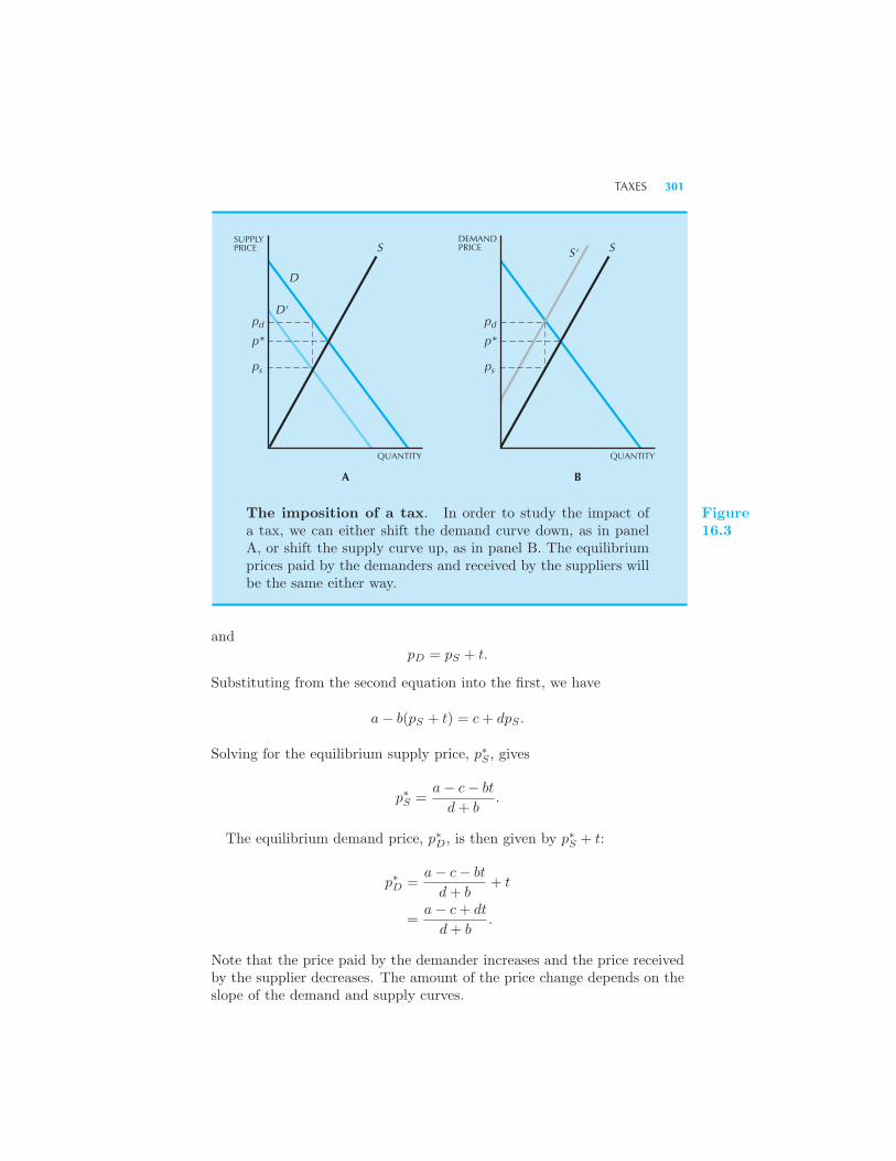
TAXES 301
SUPPLYPRICE
D
D'p
p*
p
S
QUANTITY
A
d
s sp
p*dp
QUANTITY
B
DEMANDPRICE S' S
The imposition of a tax. In order to study the impact ofa tax, we can either shift the demand curve down, as in panelA, or shift the supply curve up, as in panel B. The equilibriumprices paid by the demanders and received by the suppliers willbe the same either way.
Figure16.3
andpD = pS + t.
Substituting from the second equation into the first, we have
a− b(pS + t) = c+ dpS .
Solving for the equilibrium supply price, p∗S , gives
p∗S =a− c− bt
d+ b.
The equilibrium demand price, p∗D, is then given by p∗S + t:
p∗D =a− c− bt
d+ b+ t
=a− c+ dt
d+ b.
Note that the price paid by the demander increases and the price receivedby the supplier decreases. The amount of the price change depends on theslope of the demand and supply curves.
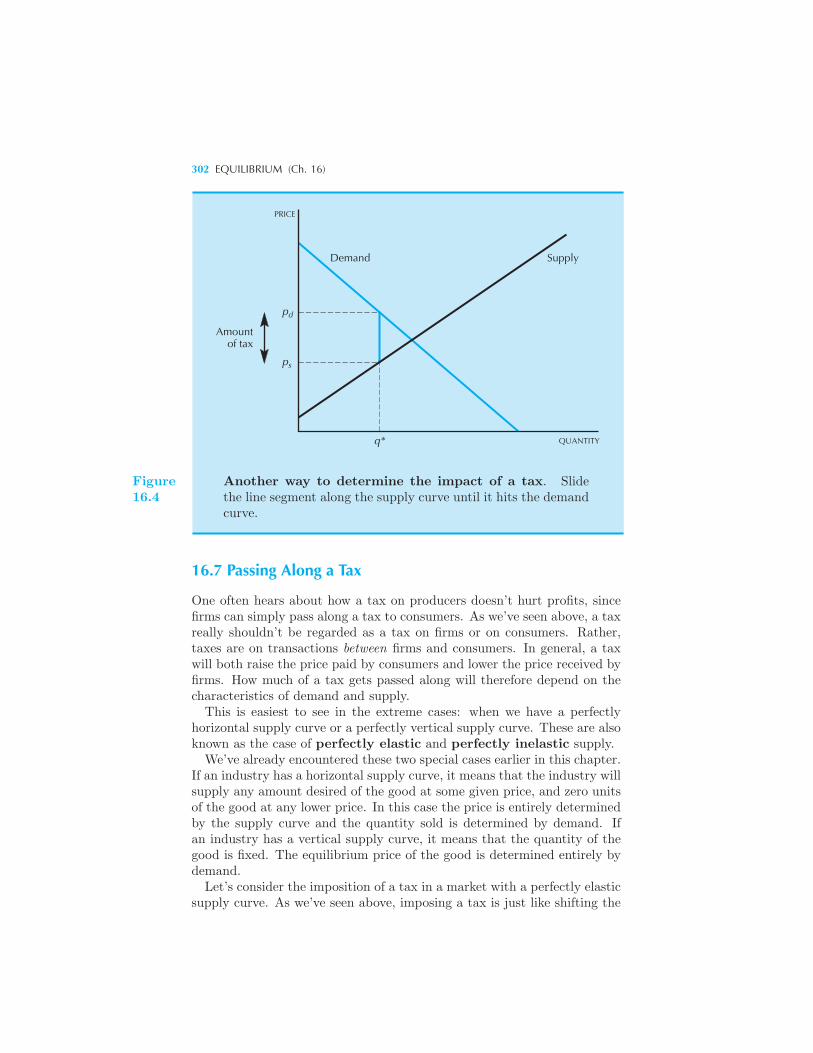
302 EQUILIBRIUM (Ch. 16)
Amountof tax
ps
pd
Demand Supply
PRICE
q* QUANTITY
Figure16.4
Another way to determine the impact of a tax. Slidethe line segment along the supply curve until it hits the demandcurve.
16.7 Passing Along a Tax
One often hears about how a tax on producers doesn’t hurt profits, sincefirms can simply pass along a tax to consumers. As we’ve seen above, a taxreally shouldn’t be regarded as a tax on firms or on consumers. Rather,taxes are on transactions between firms and consumers. In general, a taxwill both raise the price paid by consumers and lower the price received byfirms. How much of a tax gets passed along will therefore depend on thecharacteristics of demand and supply.This is easiest to see in the extreme cases: when we have a perfectly
horizontal supply curve or a perfectly vertical supply curve. These are alsoknown as the case of perfectly elastic and perfectly inelastic supply.
We’ve already encountered these two special cases earlier in this chapter.If an industry has a horizontal supply curve, it means that the industry willsupply any amount desired of the good at some given price, and zero unitsof the good at any lower price. In this case the price is entirely determinedby the supply curve and the quantity sold is determined by demand. Ifan industry has a vertical supply curve, it means that the quantity of thegood is fixed. The equilibrium price of the good is determined entirely bydemand.Let’s consider the imposition of a tax in a market with a perfectly elastic
supply curve. As we’ve seen above, imposing a tax is just like shifting the
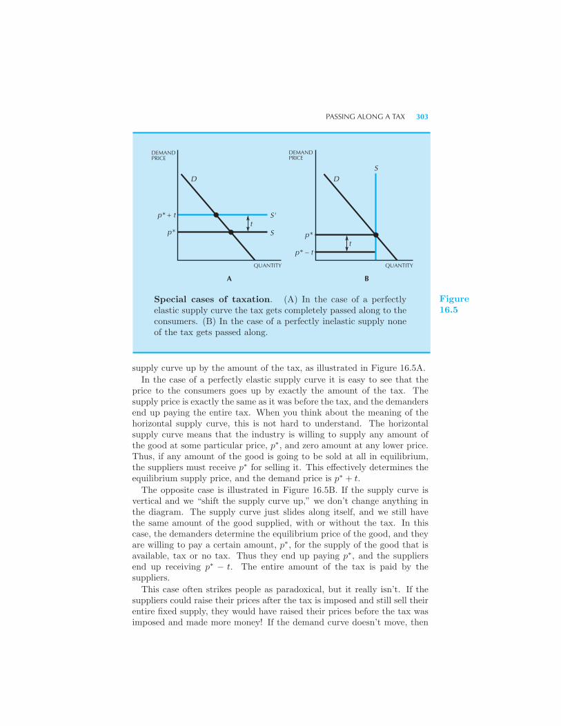
PASSING ALONG A TAX 303
DEMANDPRICE
DEMANDPRICE
D D
S'
St
tp*
p* – t
p*
p* + t
A B
QUANTITYQUANTITY
S
Special cases of taxation. (A) In the case of a perfectlyelastic supply curve the tax gets completely passed along to theconsumers. (B) In the case of a perfectly inelastic supply noneof the tax gets passed along.
Figure16.5
supply curve up by the amount of the tax, as illustrated in Figure 16.5A.
In the case of a perfectly elastic supply curve it is easy to see that theprice to the consumers goes up by exactly the amount of the tax. Thesupply price is exactly the same as it was before the tax, and the demandersend up paying the entire tax. When you think about the meaning of thehorizontal supply curve, this is not hard to understand. The horizontalsupply curve means that the industry is willing to supply any amount ofthe good at some particular price, p∗, and zero amount at any lower price.Thus, if any amount of the good is going to be sold at all in equilibrium,the suppliers must receive p∗ for selling it. This effectively determines theequilibrium supply price, and the demand price is p∗ + t.
The opposite case is illustrated in Figure 16.5B. If the supply curve isvertical and we “shift the supply curve up,” we don’t change anything inthe diagram. The supply curve just slides along itself, and we still havethe same amount of the good supplied, with or without the tax. In thiscase, the demanders determine the equilibrium price of the good, and theyare willing to pay a certain amount, p∗, for the supply of the good that isavailable, tax or no tax. Thus they end up paying p∗, and the suppliersend up receiving p∗ − t. The entire amount of the tax is paid by thesuppliers.
This case often strikes people as paradoxical, but it really isn’t. If thesuppliers could raise their prices after the tax is imposed and still sell theirentire fixed supply, they would have raised their prices before the tax wasimposed and made more money! If the demand curve doesn’t move, then
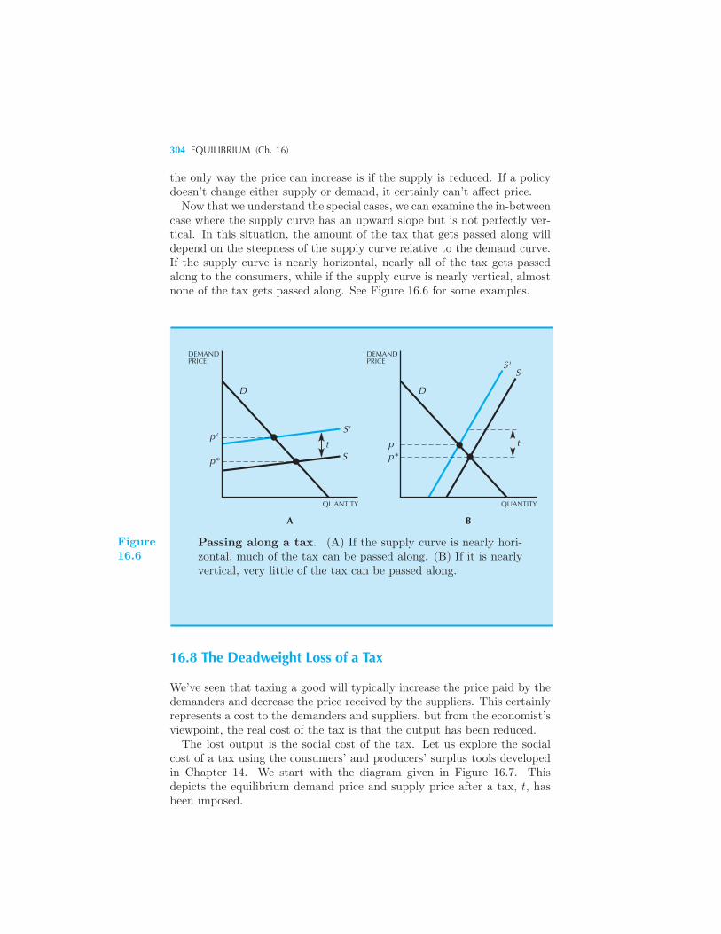
304 EQUILIBRIUM (Ch. 16)
the only way the price can increase is if the supply is reduced. If a policydoesn’t change either supply or demand, it certainly can’t affect price.Now that we understand the special cases, we can examine the in-between
case where the supply curve has an upward slope but is not perfectly ver-tical. In this situation, the amount of the tax that gets passed along willdepend on the steepness of the supply curve relative to the demand curve.If the supply curve is nearly horizontal, nearly all of the tax gets passedalong to the consumers, while if the supply curve is nearly vertical, almostnone of the tax gets passed along. See Figure 16.6 for some examples.
DEMANDPRICE
DEMANDPRICE
D D
t
S'
S
p'
p*
QUANTITY
A B
QUANTITY
S
t
S'
p*p'
Figure16.6
Passing along a tax. (A) If the supply curve is nearly hori-zontal, much of the tax can be passed along. (B) If it is nearlyvertical, very little of the tax can be passed along.
16.8 The Deadweight Loss of a Tax
We’ve seen that taxing a good will typically increase the price paid by thedemanders and decrease the price received by the suppliers. This certainlyrepresents a cost to the demanders and suppliers, but from the economist’sviewpoint, the real cost of the tax is that the output has been reduced.The lost output is the social cost of the tax. Let us explore the social
cost of a tax using the consumers’ and producers’ surplus tools developedin Chapter 14. We start with the diagram given in Figure 16.7. Thisdepicts the equilibrium demand price and supply price after a tax, t, hasbeen imposed.
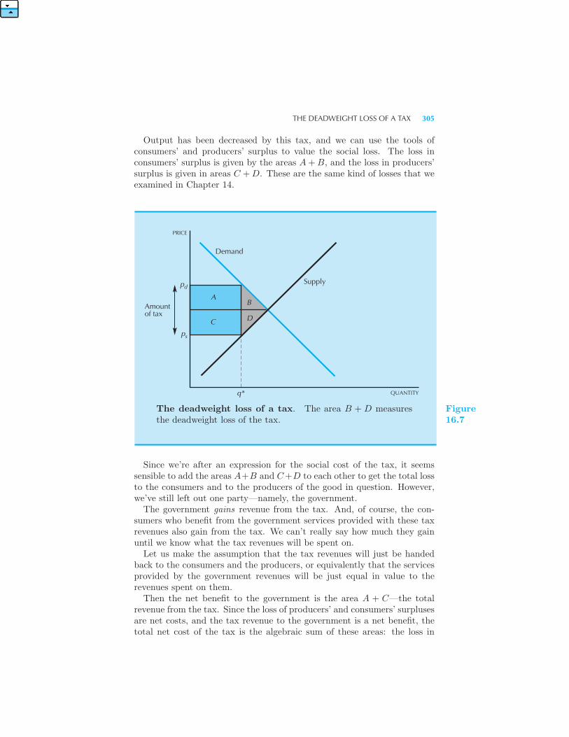
THE DEADWEIGHT LOSS OF A TAX 305
Output has been decreased by this tax, and we can use the tools ofconsumers’ and producers’ surplus to value the social loss. The loss inconsumers’ surplus is given by the areas A+B, and the loss in producers’surplus is given in areas C +D. These are the same kind of losses that weexamined in Chapter 14.
Demand
Supply
Amountof tax
PRICE
p
p
A
C
B
D
d
s
q* QUANTITY
The deadweight loss of a tax. The area B + D measuresthe deadweight loss of the tax.
Figure16.7
Since we’re after an expression for the social cost of the tax, it seemssensible to add the areas A+B and C+D to each other to get the total lossto the consumers and to the producers of the good in question. However,we’ve still left out one party—namely, the government.The government gains revenue from the tax. And, of course, the con-
sumers who benefit from the government services provided with these taxrevenues also gain from the tax. We can’t really say how much they gainuntil we know what the tax revenues will be spent on.Let us make the assumption that the tax revenues will just be handed
back to the consumers and the producers, or equivalently that the servicesprovided by the government revenues will be just equal in value to therevenues spent on them.Then the net benefit to the government is the area A + C—the total
revenue from the tax. Since the loss of producers’ and consumers’ surplusesare net costs, and the tax revenue to the government is a net benefit, thetotal net cost of the tax is the algebraic sum of these areas: the loss in
306 EQUILIBRIUM (Ch. 16)
consumers’ surplus, −(A + B), the loss in producers’ surplus, −(C + D),and the gain in government revenue, +(A+ C).The net result is the area −(B +D). This area is known as the dead-
weight loss of the tax or the excess burden of the tax. This latter phraseis especially descriptive.Recall the interpretation of the loss of consumers’ surplus. It is how
much the consumers would pay to avoid the tax. In terms of this diagramthe consumers are willing to pay A + B to avoid the tax. Similarly, theproducers are willing to pay C + D to avoid the tax. Together they arewilling to pay A + B + C +D to avoid a tax that raises A + C dollars ofrevenue. The excess burden of the tax is therefore B +D.What is the source of this excess burden? Basically it is the lost value to
the consumers and producers due to the reduction in the sales of the good.You can’t tax what isn’t there.1 So the government doesn’t get any revenueon the reduction in sales of the good. From the viewpoint of society, it isa pure loss—a deadweight loss.We could also derive the deadweight loss directly from its definition, by
just measuring the social value of the lost output. Suppose that we startat the old equilibrium and start moving to the left. The first unit lost wasone where the price that someone was willing to pay for it was just equalto the price that someone was willing to sell it for. Here there is hardlyany social loss since this unit was the marginal unit that was sold.Now move a little farther to the left. The demand price measures how
much someone was willing to pay to receive the good, and the supply pricemeasures the price at which someone was willing to supply the good. Thedifference is the lost value on that unit of the good. If we add this up overthe units of the good that are not produced and consumed because of thepresence of the tax, we get the deadweight loss.
EXAMPLE: The Market for Loans
The amount of borrowing or lending in an economy is influenced to a largedegree by the interest rate charged. The interest rate serves as a price inthe market for loans.We can let D(r) be the demand for loans by borrowers and S(r) be
the supply of loans by lenders. The equilibrium interest rate, r∗, is thendetermined by the condition that demand equal supply:
D(r∗) = S(r∗). (16.1)
Suppose we consider adding taxes to this model. What will happen tothe equilibrium interest rate?
1 At least the government hasn’t figured out how to do this yet. But they’re workingon it.
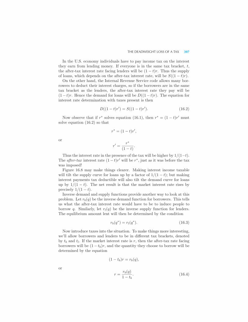
THE DEADWEIGHT LOSS OF A TAX 307
In the U.S. economy individuals have to pay income tax on the interestthey earn from lending money. If everyone is in the same tax bracket, t,the after-tax interest rate facing lenders will be (1− t)r. Thus the supplyof loans, which depends on the after-tax interest rate, will be S((1− t)r).
On the other hand, the Internal Revenue Service code allows many bor-rowers to deduct their interest charges, so if the borrowers are in the sametax bracket as the lenders, the after-tax interest rate they pay will be(1− t)r. Hence the demand for loans will be D((1− t)r). The equation forinterest rate determination with taxes present is then
D((1− t)r′) = S((1− t)r′). (16.2)
Now observe that if r∗ solves equation (16.1), then r∗ = (1 − t)r′ mustsolve equation (16.2) so that
r∗ = (1− t)r′,
or
r′ =r∗
(1− t).
Thus the interest rate in the presence of the tax will be higher by 1/(1−t).The after-tax interest rate (1− t)r′ will be r∗, just as it was before the taxwas imposed!Figure 16.8 may make things clearer. Making interest income taxable
will tilt the supply curve for loans up by a factor of 1/(1− t); but makinginterest payments tax deductible will also tilt the demand curve for loansup by 1/(1 − t). The net result is that the market interest rate rises byprecisely 1/(1− t).
Inverse demand and supply functions provide another way to look at thisproblem. Let rb(q) be the inverse demand function for borrowers. This tellsus what the after-tax interest rate would have to be to induce people toborrow q. Similarly, let rl(q) be the inverse supply function for lenders.The equilibrium amount lent will then be determined by the condition
rb(q∗) = rl(q
∗). (16.3)
Now introduce taxes into the situation. To make things more interesting,we’ll allow borrowers and lenders to be in different tax brackets, denotedby tb and tl. If the market interest rate is r, then the after-tax rate facingborrowers will be (1− tb)r, and the quantity they choose to borrow will bedetermined by the equation
(1− tb)r = rb(q),
or
r =rb(q)
1− tb. (16.4)
308 EQUILIBRIUM (Ch. 16)
LOANS
INTERESTRATE D'
D
S'
S
q*
r*
(1 – t )r*
Figure16.8
Equilibrium in the loan market. If borrowers and lendersare in the same tax bracket, the after-tax interest rate and theamount borrowed are unchanged.
Similarly, the after-tax rate facing lenders will be (1− tl)r, and the amountthey choose to lend will be determined by the equation
(1− tl)r = rl(q)
or
r =rl(q)
1− tl. (16.5)
Combining equations (16.4) and (16.5) gives the equilibrium condition:
r =rb(q)
1− tb=
rl(q)
1− tl. (16.6)
From this equation it is easy to see that if borrowers and lenders are in thesame tax bracket, so that tb = tl, then q = q∗. What if they are in differenttax brackets? It is not hard to see that the tax law is subsidizing borrowersand taxing lenders, but what is the net effect? If the borrowers face ahigher price than the lenders, then the system is a net tax on borrowing,but if the borrowers face a lower price than the lenders, then it is a netsubsidy. Rewriting the equilibrium condition, equation (16.6), we have
rb(q) =1− tb1− tl
rl(q).
THE DEADWEIGHT LOSS OF A TAX 309
Thus borrowers will face a higher price than lenders if
1− tb1− tl
> 1,
which means that tl > tb. So if the tax bracket of lenders is greater thanthe tax bracket of borrowers, the system is a net tax on borrowing, but iftl < tb, it is a net subsidy.
EXAMPLE: Food Subsidies
In years when there were bad harvests in nineteenth-century England therich would provide charitable assistance to the poor by buying up the har-vest, consuming a fixed amount of the grain, and selling the remainder tothe poor at half the price they paid for it. At first thought this seems likeit would provide significant benefits to the poor, but on second thought,doubts begin to arise.
The only way that the poor can be made better off is if they end upconsuming more grain. But there is a fixed amount of grain available afterthe harvest. So how can the poor be better off because of this policy?
As a matter of fact they are not; the poor end up paying exactly thesame price for the grain with or without the policy. To see why, we willmodel the equilibrium with and without this program. Let D(p) be thedemand curve for the poor, K the amount demanded by the rich, and Sthe fixed amount supplied in a year with a bad harvest. By assumption thesupply of grain and the demand by the rich are fixed. Without the charityprovided by the rich, the equilibrium price is determined by total demandequals total supply:
D(p∗) +K = S.
With the program in place, the equilibrium price is determined by
D(p/2) +K = S.
But now observe: if p∗ solves the first equation, then p = 2p∗ solves thesecond equation. So when the rich offer to buy the grain and distribute it tothe poor, the market price is simply bid up to twice the original price—andthe poor pay the same price they did before!
When you think about it this isn’t too surprising. If the demand of therich is fixed and the supply of grain is fixed, then the amount that thepoor can consume is fixed. Thus the equilibrium price facing the poor isdetermined entirely by their own demand curve; the equilibrium price willbe the same, regardless of how the grain is provided to the poor.
310 EQUILIBRIUM (Ch. 16)
EXAMPLE: Subsidies in Iraq
Even subsidies that are put in place “for a good reason” can be extremelydifficult to dislodge. Why? Because they create a political constituencythat comes to rely on them. This is true in every country, but Iraq repre-sents a particularly egregious case. As of 2005, fuel and food subsidies inIraq consumed nearly one third of the government’s budget.2
Almost all of the Iraqi government’s budget comes from oil exports.There is very little refining capacity in the country, so Iraq imports gasolineat 30 to 35 cents a liter, which it then sells to the public at 1.5 cents.A substantial amount of this gasoline is sold on the black market andsmuggled into Turkey, where gas is about one dollar a liter.
Food and fuel oil are also highly subsidized. Politicians are reluctant toremove these subsidies due to the politically unstable environment. Whensimilar subsidies were removed in Yemen, there was rioting in the streets,with dozens of people dying. A World Bank study concluded that morethan half of the GDP in Iraq was spent on subsidies. According to thefinance minister, Ali Abdulameer Allawi, “They’ve reached the point wherethey’ve become insane. They distort the economy in a grotesque way, andcreate the worst incentives you can think of.”
16.9 Pareto Efficiency
An economic situation is Pareto efficient if there is no way to makeany person better off without hurting anybody else. Pareto efficiency is adesirable thing—if there is some way to make some group of people betteroff, why not do it?—but efficiency is not the only goal of economic policy.For example, efficiency has almost nothing to say about income distributionor economic justice.
However, efficiency is an important goal, and it is worth asking how wella competitive market does in achieving Pareto efficiency. A competitivemarket, or any economic mechanism, has to determine two things. First,how much is produced, and second, who gets it. A competitive marketdetermines how much is produced based on how much people are willing topay to purchase the good as compared to how much people must be paidto supply the good.
Consider Figure 16.9. At any amount of output less than the competitiveamount q∗, there is someone who is willing to supply an extra unit of the
2 James Glanz, “Despite Crushing Costs, Iraqi Cabinet Lets Big Subsidies Stand,” NewYork Times, August 11, 2005.
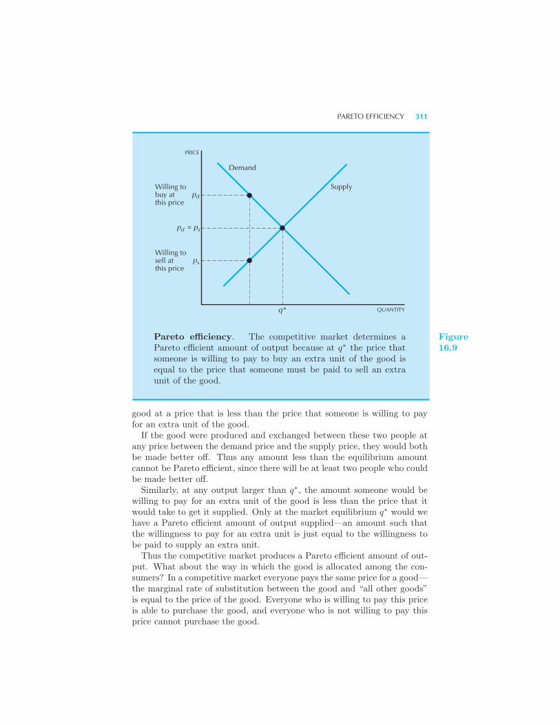
PARETO EFFICIENCY 311
PRICE
Demand
Supplyp
p = p
p
Willing tobuy atthis price
Willing tosell atthis price
q* QUANTITY
d s
s
d
Pareto efficiency. The competitive market determines aPareto efficient amount of output because at q∗ the price thatsomeone is willing to pay to buy an extra unit of the good isequal to the price that someone must be paid to sell an extraunit of the good.
Figure16.9
good at a price that is less than the price that someone is willing to payfor an extra unit of the good.If the good were produced and exchanged between these two people at
any price between the demand price and the supply price, they would bothbe made better off. Thus any amount less than the equilibrium amountcannot be Pareto efficient, since there will be at least two people who couldbe made better off.Similarly, at any output larger than q∗, the amount someone would be
willing to pay for an extra unit of the good is less than the price that itwould take to get it supplied. Only at the market equilibrium q∗ would wehave a Pareto efficient amount of output supplied—an amount such thatthe willingness to pay for an extra unit is just equal to the willingness tobe paid to supply an extra unit.Thus the competitive market produces a Pareto efficient amount of out-
put. What about the way in which the good is allocated among the con-sumers? In a competitive market everyone pays the same price for a good—the marginal rate of substitution between the good and “all other goods”is equal to the price of the good. Everyone who is willing to pay this priceis able to purchase the good, and everyone who is not willing to pay thisprice cannot purchase the good.
312 EQUILIBRIUM (Ch. 16)
What would happen if there were an allocation of the good where themarginal rates of substitution between the good and “all other goods” werenot the same? Then there must be at least two people who value a marginalunit of the good differently. Maybe one values a marginal unit at $5 andone values it at $4. Then if the one with the lower value sells a bit of thegood to the one with the higher value at any price between $4 and $5,both people would be made better off. Thus any allocation with differentmarginal rates of substitution cannot be Pareto efficient.
EXAMPLE: Waiting in Line
One commonly used way to allocate resources is by making people waitin line. We can analyze this mechanism for resource allocation using thesame tools that we have developed for analyzing the market mechanism.Let us look at a concrete example: suppose that your university is going todistribute tickets to the championship basketball game. Each person whowaits in line can get one ticket for free.The cost of a ticket will then simply be the cost of waiting in line. People
who want to see the basketball game very much will camp out outside theticket office so as to be sure to get a ticket. People who don’t care verymuch about the game may drop by a few minutes before the ticket windowopens on the off chance that some tickets will be left. The willingness to payfor a ticket should no longer be measured in dollars but rather in waitingtime, since tickets will be allocated according to willingness to wait.Will waiting in line result in a Pareto efficient allocation of tickets? Ask
yourself whether it is possible that someone who waited for a ticket mightbe willing to sell it to someone who didn’t wait in line. Often this will bethe case, simply because willingness to wait and willingness to pay differacross the population. If someone is willing to wait in line to buy a ticketand then sell it to someone else, allocating tickets by willingness to waitdoes not exhaust all the gains to trade—some people would generally stillbe willing to trade the tickets after the tickets have been allocated. Sincewaiting in line does not exhaust all of the gains from trade, it does not ingeneral result in a Pareto efficient outcome.If you allocate a good using a price set in dollars, then the dollars paid by
the demanders provide benefits to the suppliers of the good. If you allocatea good using waiting time, the hours spent in line don’t benefit anybody.The waiting time imposes a cost on the buyers of the good and providesno benefits at all to the suppliers. Waiting in line is a form of deadweightloss—the people who wait in line pay a “price” but no one else receivesany benefits from the price they pay.

REVIEW QUESTIONS 313
Summary
1. The supply curve measures how much people will be willing to supplyof some good at each price.
2. An equilibrium price is one where the quantity that people are willingto supply equals the quantity that people are willing to demand.
3. The study of how the equilibrium price and quantity change when theunderlying demand and supply curves change is another example of com-parative statics.
4. When a good is taxed, there will always be two prices: the price paidby the demanders and the price received by the suppliers. The differencebetween the two represents the amount of the tax.
5. How much of a tax gets passed along to consumers depends on therelative steepness of the demand and supply curves. If the supply curveis horizontal, all of the tax gets passed along to consumers; if the supplycurve is vertical, none of the tax gets passed along.
6. The deadweight loss of a tax is the net loss in consumers’ surplus plusproducers’ surplus that arises from imposing the tax. It measures the valueof the output that is not sold due to the presence of the tax.
7. A situation is Pareto efficient if there is no way to make some group ofpeople better off without making some other group worse off.
8. The Pareto efficient amount of output to supply in a single market isthat amount where the demand and supply curves cross, since this is theonly point where the amount that demanders are willing to pay for an extraunit of output equals the price at which suppliers are willing to supply anextra unit of output.
REVIEW QUESTIONS
1. What is the effect of a subsidy in a market with a horizontal supplycurve? With a vertical supply curve?
2. Suppose that the demand curve is vertical while the supply curve slopesupward. If a tax is imposed in this market who ends up paying it?
314 EQUILIBRIUM (Ch. 16)
3. Suppose that all consumers view red pencils and blue pencils as perfectsubstitutes. Suppose that the supply curve for red pencils is upward slop-ing. Let the price of red pencils and blue pencils be pr and pb. What wouldhappen if the government put a tax only on red pencils?
4. The United States imports about half of its petroleum needs. Supposethat the rest of the oil producers are willing to supply as much oil as theUnited States wants at a constant price of $25 a barrel. What would happento the price of domestic oil if a tax of $5 a barrel were placed on foreignoil?
5. Suppose that the supply curve is vertical. What is the deadweight lossof a tax in this market?
6. Consider the tax treatment of borrowing and lending described in thetext. How much revenue does this tax system raise if borrowers and lendersare in the same tax bracket?
7. Does such a tax system raise a positive or negative amount of revenuewhen tl < tb?
CHAPTER 17
MEASUREMENT
Up until now we have used simple algebraic expressions to describe util-ity functions, production functions, demand curves, supply curves, and soon. For actual applications we have to estimate these functions using sta-tistical techniques. The study of how to do this effectively is known aseconometrics.When we analyze data we generally are concerned with the following
questions.
Summarize. How can we describe the data succinctly? Example: howmany cups of coffee are consumed per person per day?
Estimate. How can we estimate some unknown parameters? Example:what is the elasticity of demand for coffee?
Test. How can we determine whether an unknown parameter satisfies somerestriction? Example: do men and women drink the same amount of coffeeper day on average?
Forecast. How can we forecast what the price of coffee will be next year?
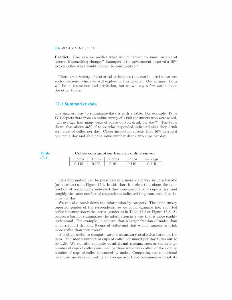
316 MEASUREMENT (Ch. 17)
Predict. How can we predict what would happen to some variable ofinterest if something changes? Example: if the government imposed a 10%tax on coffee what would happen to consumption?
There are a variety of statistical techniques that can be used to answersuch questions, which we will explore in this chapter. Our primary focuswill be on estimation and prediction, but we will say a few words aboutthe other topics.
17.1 Summarize data
The simplest way to summarize data is with a table. For example, Table17.1 depicts data from an online survey of 1,000 consumers who were asked,“On average how many cups of coffee do you drink per day?” The tableshows that about 45% of those who responded indicated that they drinkzero cups of coffee per day. Closer inspection reveals that 16% averagedone cup a day and about the same number drank two cups per day.
Table17.1
Coffee consumption from an online survey
0 cups 1 cup 2 cups 3 cups 4+ cups0.448 0.163 0.161 0.110 0.119
This information can be presented in a more vivid way using a barplot(or barchart) as in Figure 17.1. In this chart it is clear that about the samefraction of respondents indicated they consumed 1 or 2 cups a day, androughly the same number of respondents indicated they consumed 3 or 4+cups per day.We can also break down the information by category. The same survey
reported gender of the respondents, so we could examine how reportedcoffee consumption varies across gender as in Table 17.2 or Figure 17.2. Asbefore, a barplot summarizes the information in a way that is more readilyunderstood. For example, it appears that a larger fraction of males thanfemales report drinking 0 cups of coffee and that woman appear to drinkmore coffee than men overall.It is often useful to compute various summary statistics based on the
data. The mean number of cups of coffee consumed per day turns out tobe 1.28. We can also compute conditional means, such as the averagenumber of cups of coffee consumed by those who drink coffee, or the averagenumber of cups of coffee consumed by males. Computing the conditionalmean just involves computing an average over those consumers who satisfy
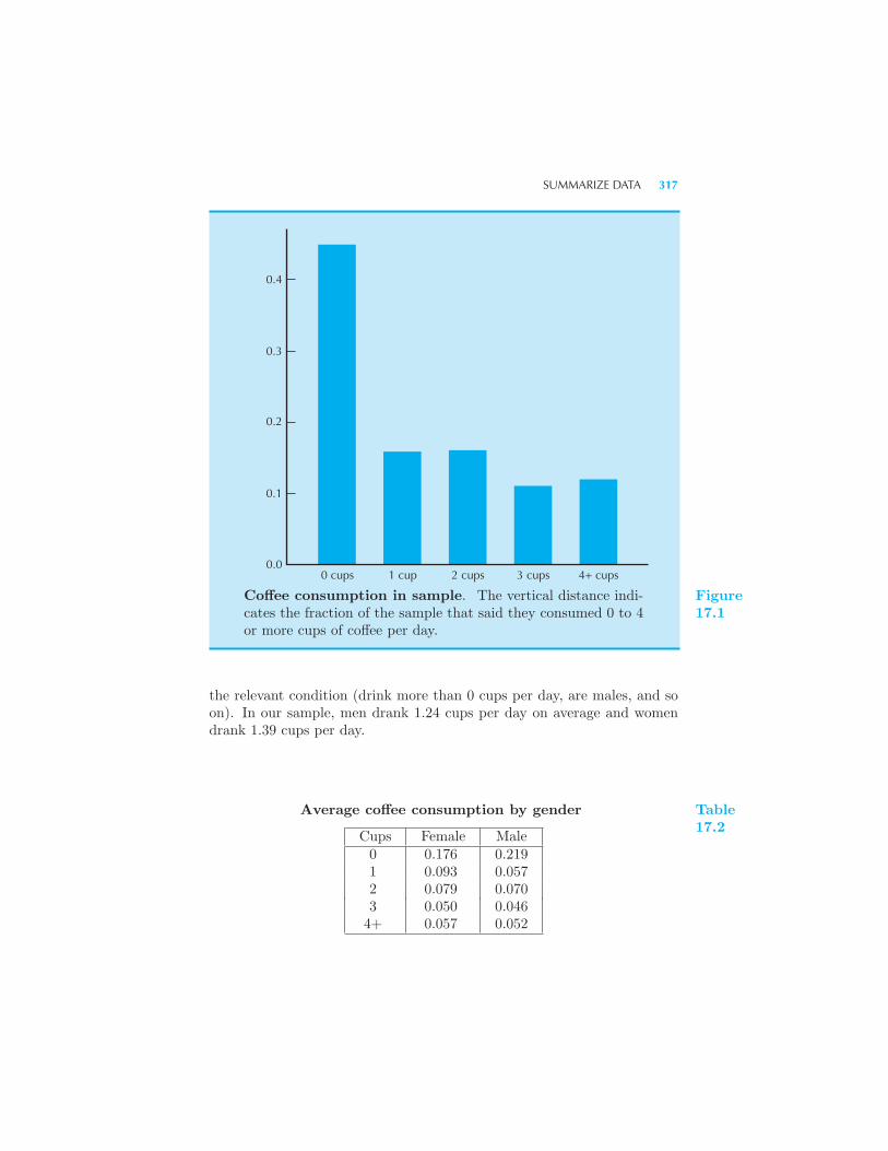
SUMMARIZE DATA 317
0 cups
0.4
0.3
0.2
0.1
0.01 cup 2 cups 3 cups 4+ cups
Coffee consumption in sample. The vertical distance indi-cates the fraction of the sample that said they consumed 0 to 4or more cups of coffee per day.
Figure17.1
the relevant condition (drink more than 0 cups per day, are males, and soon). In our sample, men drank 1.24 cups per day on average and womendrank 1.39 cups per day.
Average coffee consumption by gender
Cups Female Male0 0.176 0.2191 0.093 0.0572 0.079 0.0703 0.050 0.0464+ 0.057 0.052
Table17.2
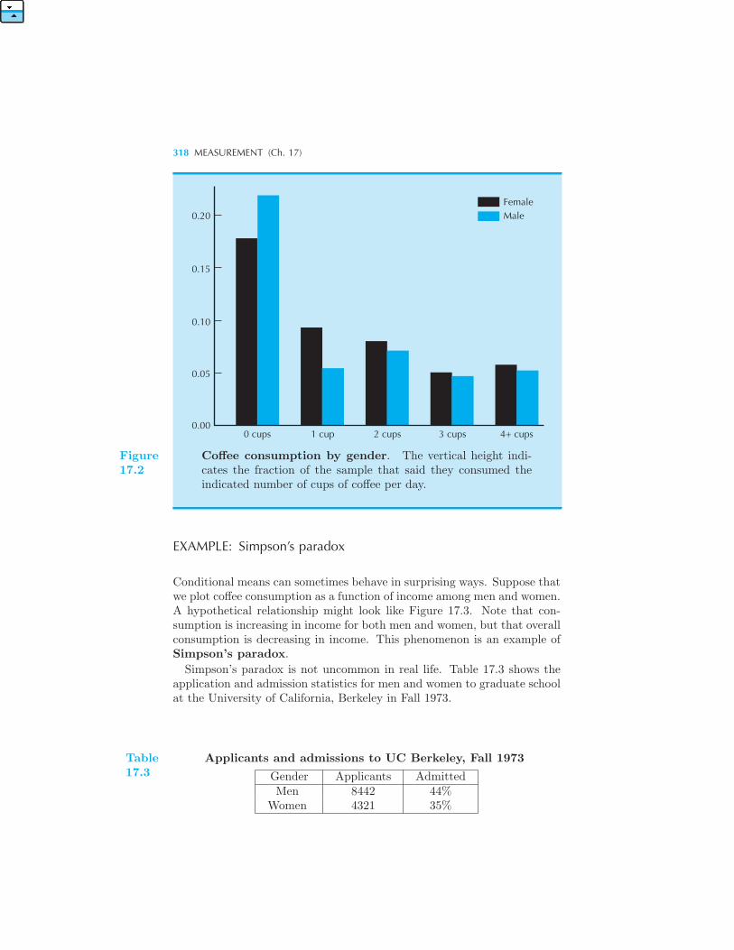
318 MEASUREMENT (Ch. 17)
0 cups
0.20
0.15
0.10
0.05
0.001 cup 2 cups
FemaleMale
3 cups 4+ cups
Figure17.2
Coffee consumption by gender. The vertical height indi-cates the fraction of the sample that said they consumed theindicated number of cups of coffee per day.
EXAMPLE: Simpson’s paradox
Conditional means can sometimes behave in surprising ways. Suppose thatwe plot coffee consumption as a function of income among men and women.A hypothetical relationship might look like Figure 17.3. Note that con-sumption is increasing in income for both men and women, but that overallconsumption is decreasing in income. This phenomenon is an example ofSimpson’s paradox.
Simpson’s paradox is not uncommon in real life. Table 17.3 shows theapplication and admission statistics for men and women to graduate schoolat the University of California, Berkeley in Fall 1973.
Table17.3
Applicants and admissions to UC Berkeley, Fall 1973
Gender Applicants AdmittedMen 8442 44%
Women 4321 35%
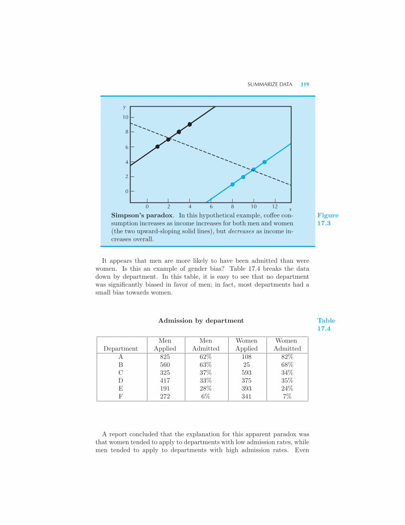
SUMMARIZE DATA 319
0 2
10
8
6
4
2
0
4 6 8 x
y
10 12
Simpson’s paradox. In this hypothetical example, coffee con-sumption increases as income increases for both men and women(the two upward-sloping solid lines), but decreases as income in-creases overall.
Figure17.3
It appears that men are more likely to have been admitted than werewomen. Is this an example of gender bias? Table 17.4 breaks the datadown by department. In this table, it is easy to see that no departmentwas significantly biased in favor of men; in fact, most departments had asmall bias towards women.
Admission by department
Men Men Women WomenDepartment Applied Admitted Applied Admitted
A 825 62% 108 82%B 560 63% 25 68%C 325 37% 593 34%D 417 33% 375 35%E 191 28% 393 24%F 272 6% 341 7%
Table17.4
A report concluded that the explanation for this apparent paradox wasthat women tended to apply to departments with low admission rates, whilemen tended to apply to departments with high admission rates. Even
320 MEASUREMENT (Ch. 17)
though there was no evidence of bias at a department level, the overallstatistics gave an impression of bias.1
17.2 Test
In the previous section we saw that men drank 1.23 cups of coffee per dayon average and women drank 1.39 cups per day on average. But this isjust one particular sample of a thousand consumers. If we took a differentsample, we would find different numbers. How confident can we be thatthe mean consumption of coffee by women exceeds the mean consumptionof coffee by men in the entire population?One way to answer this question is to pose it in the following way. Sup-
pose that men and women actually drank the same amount of coffee perday. How likely would it be in a particular sample of 1,000 consumers toobserve one group drinking 1.39− 1.23 = 0.16 cups more than the other?In our sample, it turns out that with a few additional assumptions the
probability that we would see a difference at least this large is about 9.6%.In other words, if men and women had the same average consumption inthe population, we would see an estimated difference of this magnitudeor larger in roughly 1 out of 10 samples. Even though our sample showsthat coffee consumption is somewhat different between men and women,we can’t be confident that this relationship holds for the population as awhole.
17.3 Estimating demand using experimental data
Suppose you work for a company that sells coffee beans via a website. Yourcoffee currently sells for $15 a pound, but you are contemplating cuttingthe price to $14. You hope that you will sell more coffee at the lower price,but how much more? Is it worth cutting your price to get more sales?In this case it is natural to run an experiment to see how the demand
for coffee changes when the price changes. For example, you could cut theprice of the coffee for a few weeks and see how much additional coffee yousell. If your profit goes up, it might make sense to make the sale pricepermanent.Another possibility would be to put the coffee on sale in just a few
states or cities and see what happens in those locations. If we try thisexperiment, it is important to recognize that there are other factors thataffect the demand for coffee than just the price. For example, the amount
1 P. J. Bickel, E. A. Hammel and J. W. O’Connell (1975). “Sex Bias in GraduateAdmissions: Data from Berkeley.” Science 187 (4175): 398-404.
EFFECT OF TREATMENT 321
of coffee you sell in a given region during a given period could vary withthe season of the year or with the weather.Ideally, you would choose which cities are treated using some random
method such as a coin flip. Such randomized treatment helps eliminatesources of systematic bias.It would also be a good idea to think about ways you could control for
these systematic effects. For example, you could compare the sales in thecities where you cut the price to sales in those cities where you kept theprice constant. Or you could collect data on weather in the cities youexamine and use statistical techniques to control for the observed variationin weather.In the language of statistics, the cities where you reduce the price of coffee
is your treatment group and the cities where you leave the price of coffeeconstant is your control group. Running the experiment is simply a small-scale version of the policy you are thinking about implementing—namely,cutting the price for everyone. If you make the experiment as much like theproposed policy as possible, then the experiment will probably give you apretty good idea about what would happen if you scaled the experimentup to the entire country.
17.4 Effect of treatment
Another thing you could do to estimate how the demand for coffee wouldrespond to a price cut is to send out coupons to a randomly chosen set ofpeople and see how many people use these coupons to buy coffee.The trouble with this procedure is that the people who redeem the
coupons may be different from the population at large. It is likely thatpeople who go to the trouble of using the coupons might be more price-sensitive on average than those who don’t bother to use the coupons.In the case of a coupon, some fraction of the population (the coupon
users) are choosing to receive a lower price rather than simply facing alower price for coffee. In general, those who choose to be treated arethose who are more interested in the treatment and may be more likelyto respond to it differently than the population as whole. So the impactof the treatment (the coupon) on those who choose to use it (the treated)could be quite different than the impact of a price cut for everyone.On the other hand, sometimes you might be interested in the “effect of
the treatment on the treated,” as opposed to the effect of treatment onthe population. For example, if the policy you had in mind was sendingout coupons to the entire population, then an experiment that involvedsending out coupons to a subset of the population would be an appropriateexperiment.The key issue is whether the consumers are making a choice of whether
or not to be treated (that is, to get the lower price). Ideally, the experiment
322 MEASUREMENT (Ch. 17)
will mimic the proposed policy as closely as possible.
17.5 Estimating demand using observational data
Let us now consider a different situation. Suppose now you are interestedin estimating how the nationwide demand for coffee in the United Stateschanges as the price changes. In this case there is no obvious way to do anexperiment. Since you don’t have experimental data, you have to useobservational data.
The statistical tool that economists use most commonly to address prob-lems of this sort is called regression. A regression is simply a way toexpress conditional expectations. For example, a regression could describethe expected consumption of coffee by a randomly chosen consumer, con-ditional on the consumer being female. When we estimate a regression weare trying to describe the relationship between a variable of interest (in ourcase coffee consumption) and other characteristics, such as gender, income,age, price, and so on. There are many varieties of regression, but we willfocus on the simplest form, which is called ordinary least squares orOLS.So suppose we are given some data on prices and quantity sold of coffee
at different time periods. How can we use this data to estimate a demandfunction?It is important to think about the data generation process: how was
this data produced? We can apply some of the theory developed in earlierchapters on consumer choice.Think of a consumer as purchasing two things, coffee (x1) and “all other
goods” (x2). Good 2 is sometimes referred to as a composite commodityor quantity index, as described in Chapter 7.Denote the price of coffee by p1, the price of “all other goods” by p2, and
the total expenditure by m. The utility maximization problem for a singleconsumer is
maxx1,x2
u(x1, x2)
such that p1x1 + p2x2 = m.
We can write the demand function for coffee as
x1 = D(p1, p2,m).
As mentioned in section 2.4, we can multiply prices and income by anypositive constant and demand stays the same. So let us multiply pricesand income by 1/p2. This gives us
x1 = D(p1/p2, 1,m/p2).
ESTIMATING DEMAND USING OBSERVATIONAL DATA 323
This says the demand for coffee is a function of the price of coffee relativeto the price of all other goods and income relative to the price of all othergoods. In practice, we compute these numbers by using a price index, likethe Consumer Price Index (CPI) or Personal Consumption Expenditureprice index (PCEPI). (See the discussion in Chapter 7 on index numbersto see how these are constructed.)Now we can add up demand across all consumers to get aggregate de-
mand. In order to avoid additional notation, we will use the same notationas above to write x = D(p,m), where x is now the aggregate demand forcoffee, p is the price of coffee divided by the CPI, m is total consumerexpenditure divided by the CPI, and D(p,m) is the aggregate demandfunction.
Functional form
We now need to pick an algebraic formula for the demand function. Thereare three forms for demand functions commonly used in practice.
Linear demand. x = c+ bp+ dm.
Log-linear demand. log (x) = log (c) + blog (p) + dlog (m).
Semi-log demand. log (x) = c+ bp+ dm.
The most popular form is log-linear demand, since it is easy to inter-pret the coefficients. As we have seen in Chapter 15, section 8, b and dmeasure the price and income elasticity of demand, respectively. (In theseexpressions, all logarithms are natural logarithms.)
Statistical model
Of course, we would not expect our model to fit perfectly, so we need toadd an error term, denoted by et. The error term measures the differencebetween our ideal specification of demand and the actual observed demand.It can be interpreted as the cumulative effect of all the omitted, unobservedvariables that affect demand.So our final specification of the data-generating process is
log (xt) = log (c) + b log (pt) + d log (mt) + et,
where the error term is interpreted as the aggregate of all the other variablesthat might be correlated with coffee consumption.
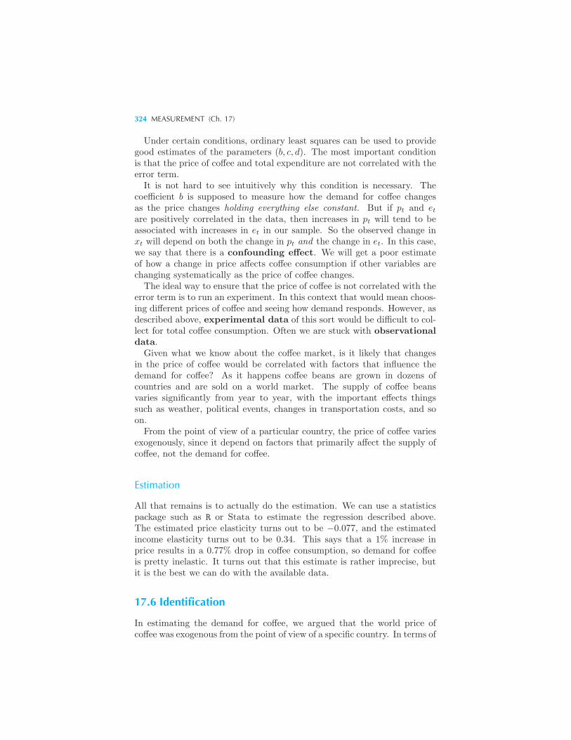
324 MEASUREMENT (Ch. 17)
Under certain conditions, ordinary least squares can be used to providegood estimates of the parameters (b, c, d). The most important conditionis that the price of coffee and total expenditure are not correlated with theerror term.It is not hard to see intuitively why this condition is necessary. The
coefficient b is supposed to measure how the demand for coffee changesas the price changes holding everything else constant. But if pt and etare positively correlated in the data, then increases in pt will tend to beassociated with increases in et in our sample. So the observed change inxt will depend on both the change in pt and the change in et. In this case,we say that there is a confounding effect. We will get a poor estimateof how a change in price affects coffee consumption if other variables arechanging systematically as the price of coffee changes.The ideal way to ensure that the price of coffee is not correlated with the
error term is to run an experiment. In this context that would mean choos-ing different prices of coffee and seeing how demand responds. However, asdescribed above, experimental data of this sort would be difficult to col-lect for total coffee consumption. Often we are stuck with observationaldata.
Given what we know about the coffee market, is it likely that changesin the price of coffee would be correlated with factors that influence thedemand for coffee? As it happens coffee beans are grown in dozens ofcountries and are sold on a world market. The supply of coffee beansvaries significantly from year to year, with the important effects thingssuch as weather, political events, changes in transportation costs, and soon.From the point of view of a particular country, the price of coffee varies
exogenously, since it depend on factors that primarily affect the supply ofcoffee, not the demand for coffee.
Estimation
All that remains is to actually do the estimation. We can use a statisticspackage such as R or Stata to estimate the regression described above.The estimated price elasticity turns out to be −0.077, and the estimatedincome elasticity turns out to be 0.34. This says that a 1% increase inprice results in a 0.77% drop in coffee consumption, so demand for coffeeis pretty inelastic. It turns out that this estimate is rather imprecise, butit is the best we can do with the available data.
17.6 Identification
In estimating the demand for coffee, we argued that the world price ofcoffee was exogenous from the point of view of a specific country. In terms of
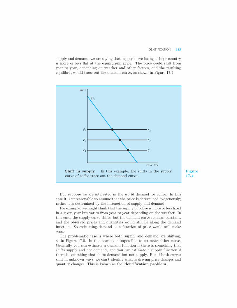
IDENTIFICATION 325
supply and demand, we are saying that supply curve facing a single countryis more or less flat at the equilibrium price. The price could shift fromyear to year, depending on weather and other factors, and the resultingequilibria would trace out the demand curve, as shown in Figure 17.4.
P3
D1
S3
P2 S2
P1 S1
PRICE
QUANTITY
Shift in supply. In this example, the shifts in the supplycurve of coffee trace out the demand curve.
Figure17.4
But suppose we are interested in the world demand for coffee. In thiscase it is unreasonable to assume that the price is determined exogenously;rather it is determined by the interaction of supply and demand.For example, we might think that the supply of coffee is more or less fixed
in a given year but varies from year to year depending on the weather. Inthis case, the supply curve shifts, but the demand curve remains constant,and the observed prices and quantities would still lie along the demandfunction. So estimating demand as a function of price would still makesense.The problematic case is where both supply and demand are shifting,
as in Figure 17.5. In this case, it is impossible to estimate either curve.Generally you can estimate a demand function if there is something thatshifts supply and not demand, and you can estimate a supply function ifthere is something that shifts demand but not supply. But if both curvesshift in unknown ways, we can’t identify what is driving price changes andquantity changes. This is known as the identification problem.
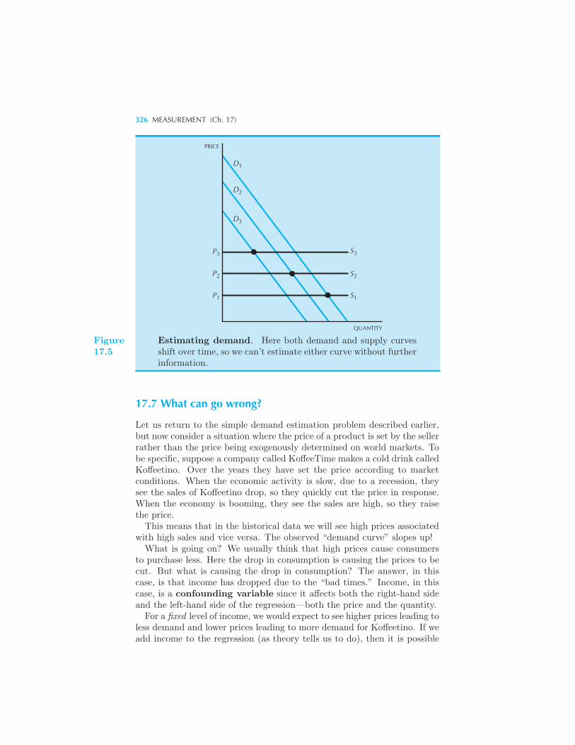
326 MEASUREMENT (Ch. 17)
P3
D2
D1
D3
S3
P2 S2
P1 S1
PRICE
QUANTITY
Figure17.5
Estimating demand. Here both demand and supply curvesshift over time, so we can’t estimate either curve without furtherinformation.
17.7 What can go wrong?
Let us return to the simple demand estimation problem described earlier,but now consider a situation where the price of a product is set by the sellerrather than the price being exogenously determined on world markets. Tobe specific, suppose a company called KoffeeTime makes a cold drink calledKoffeetino. Over the years they have set the price according to marketconditions. When the economic activity is slow, due to a recession, theysee the sales of Koffeetino drop, so they quickly cut the price in response.When the economy is booming, they see the sales are high, so they raisethe price.This means that in the historical data we will see high prices associated
with high sales and vice versa. The observed “demand curve” slopes up!What is going on? We usually think that high prices cause consumers
to purchase less. Here the drop in consumption is causing the prices to becut. But what is causing the drop in consumption? The answer, in thiscase, is that income has dropped due to the “bad times.” Income, in thiscase, is a confounding variable since it affects both the right-hand sideand the left-hand side of the regression—both the price and the quantity.For a fixed level of income, we would expect to see higher prices leading to
less demand and lower prices leading to more demand for Koffeetino. If weadd income to the regression (as theory tells us to do), then it is possible
POLICY EVALUATION 327
that we will get a meaningful estimate of price elasticity In econometriclanguage, this is an example ofmissing variable bias: we failed to includean important variable in the regression and so we got a biased estimate ofthe effect.But, in reality, there are always omitted variables—we can never have a
complete list of everything that affects demand. For example, it may bethat weather affects Koffeetino. In years with particularly cold tempera-tures sales fall and in warm years sales rise. The company may respond byraising or lowering price in response to the change in sales, leading to thesame problem we had before.As mentioned earlier, omitted variables that are not correlated with price
are not much of a problem. But omitted variables that are correlated withprice (confounding variables) can result in biased estimates. This will oftenbe the case when the price is chosen, since the choice may depend on lotsof things that the econometrician may not subsequently observe.As it turns out, there are ways to address this problem that are covered in
more advanced courses. Experiments are the gold standard, but sometimesobservational data can be used to estimate causal effects even withoutexplicit experiments.
17.8 Policy evaluation
A common reason to estimate the magnitude of some effect is that we arecontemplating some policy change. Ideally, we would run an experimenton a small scale to estimate the impact of the proposed change. But, aswe have seen, it is sometimes difficult or costly to run such an experiment.Sometimes we can find a natural experiment that is similar to the
ideal experiment we would run if we could. For example, in 2008 theState of Oregon ran a lottery among low-income adults to determine whowould be allowed to apply for Medicare. A year after this lottery, thetreatment group—those who were allowed to apply for Medicare—weresubstantially more likely to be covered by health insurance than those whoweren’t allowed to apply.2
The researchers were able to see how the treated group differed fromthe control group. In the first year of the study, it turned out that thetreated group had higher health care utilization, lower out-of-pocket med-ical expenditures and medical debt, and better self-reported physical andmental health than the control group. One might reasonably expect thatthis would carry over to larger populations who were offered the chance tosign up for Medicare.
2 Amy Finkelstein et. al., “The Oregon Health Insurance Experiment: Evidence fromthe First Year,” http://economics.mit.edu/files/6796.
328 MEASUREMENT (Ch. 17)
Of course, offering people the opportunity to sign up for Medicare isdifferent from extending it to the entire population. In the first case, peoplestill choose to apply and those who apply could be different from the entirepopulation in relevant ways.
EXAMPLE: Crime and police
It is important to distinguish correlation and causation. A classic example:if we observe more police in precincts with high crime rates, can we concludethat police cause crime? Of course not. A more likely explanation is thatthe causality runs the other direction: more police were assigned to highcrime areas because they had high crime.If we use statistical procedures to estimate the relationship between num-
bers of police and crime rates, we may well see a positive relationship(more police are associated with more crime). However, that says nothingabout what would happen if we deliberately assigned more police to a givenprecinct.In order to understand the causal impact of police on crime rates, we need
to understand (1) how police were assigned to precincts in the historicaldata and (2) how the assignment of additional police to a given precinctchanges crime rates.Ideally we would use a controlled experiment to determine how the num-
ber of police affects crime rates. However, sometimes there might be a“natural experiment” that mimics such a random assignment. For exam-ple, the police department in Washington, DC, increases the number ofpolice on the street during periods when there are security alerts concern-ing elevated risk of terrorist activity. Two economists examined the dataon crime reports for these days and found that crime was substantiallylower, particularly for auto theft.3
Summary
1. Statistics can be used to summarize, estimate, test, and predict.
2. Omitted variable bias occurs when the analyst fails to include an im-portant variable in the regression that is correlated with other variables.In this case the omitted variable is known as a confounding variable.
3. Observational data can only tell us about correlations, but we normallyneed experiments to determine causality.
3 Jonathan Klick and Alexander Tababrok, “Using Terror Alert Levels to Estimate theEffect of Police on Crime,” Journal of Law and Economics 48:1 (April 2005), 267–79.

REVIEW QUESTIONS 329
4. However, in some cases there are natural experiments that can be usefulin answering questions of interest.
5. It is important to distinguish between the effect of a policy that appliesto the entire population and the effect of a policy that applies only to thosewho choose to participate.
6. In general, in evaluating a policy proposal, the experiment used shouldbe as close as possible to the policy being considered.
REVIEW QUESTIONS
1. When the Titanic sank in 1912, both male and female crew membershad a higher survival rate than the third-class passengers. However, overallthe third-class passengers had a higher survival rate than the crew. Whatdo we call this phenomenon?
2. Suppose that you want to test the hypothesis that a coin has a probabilityof 1/2 of coming up heads when you flip it. You flip it 5 times and it comesup heads every time. How likely is it that you would see a pattern of 5heads in a row if true probability of coming up heads is 1/2?
3. Suppose we estimate a demand function of the form x = ec+bp, wherep is price, x is the quantity consumed, and b is a parameter. What is thisfunctional form called?
CHAPTER 18
AUCTIONS
Auctions are one of the oldest form of markets, dating back to at least 500BC. Today, all sorts of commodities, from used computers to fresh flowers,are sold using auctions.Economists became interested in auctions in the early 1970s when the
OPEC oil cartel raised the price of oil. The U.S. Department of the Inte-rior decided to hold auctions to sell the right to drill in coastal areas thatwere expected to contain vast amounts of oil. The government asked econ-omists how to design these auctions, and private firms hired economists asconsultants to help them design a bidding strategy. This effort promptedconsiderable research in auction design and strategy.More recently, the Federal Communications Commission (FCC) decided
to auction off parts of the radio spectrum for use by cellular phones, per-sonal digital assistants, and other communication devices. Again, econ-omists played a major role in the design of both the auctions and thestrategies used by the bidders. These auctions were hailed as very suc-cessful public policy, resulting in revenues to the U.S. government of overtwenty-three billion dollars to date.Other countries have also used auctions for privatization projects. For
example, Australia sold off several government-owned electricity plants,and New Zealand auctioned off parts of its state-owned telephone system.
CLASSIFICATION OF AUCTIONS 331
Consumer-oriented auctions have also experienced something of a re-naissance on the Internet. There are hundreds of auctions on the Internet,selling collectibles, computer equipment, travel services, and other items.OnSale claims to be the largest, reporting over forty-one million dollarsworth of merchandise sold in 1997.
18.1 Classification of Auctions
The economic classification of auctions involves two considerations: first,what is the nature of the good that is being auctioned, and second, whatare the rules of bidding? With respect to the nature of the good, econo-mists distinguish between private-value auctions and common-valueauctions.In a private-value auction, each participant has a potentially different
value for the good in question. A particular piece of art may be worth$500 to one collector, $200 to another, and $50 to yet another, dependingon their taste. In a common-value auction, the good in question is worthessentially the same amount to every bidder, although the bidders mayhave different estimates of that common value. The auction for off-shoredrilling rights described above had this characteristic: a given tract eitherhad a certain amount of oil or not. Different oil companies may have haddifferent estimates about how much oil was there, based on the outcomes oftheir geological surveys, but the oil had the same market value regardlessof who won the auction.We will spend most of the time in this chapter discussing private-value
auctions, since they are the most familiar case. At the end of the chapter,we will describe some of the features of common-value auctions.
Bidding Rules
The most prevalent form of bidding structure for an auction is the Englishauction. The auctioneer starts with a reserve price, which is the lowestprice at which the seller of the good will part with it.1 Bidders successivelyoffer higher prices; generally each bid must exceed the previous bid by someminimal bid increment. When no participant is willing to increase thebid further, the item is awarded to the highest bidder.Another form of auction is known as a Dutch auction, due to its use
in the Netherlands for selling cheese and fresh flowers. In this case theauctioneer starts with a high price and gradually lowers it by steps untilsomeone is willing to buy the item. In practice, the “auctioneer” is often
1 See the footnote about “reservation price” in Chapter 6, which is essentially the sameconcept.
332 AUCTIONS (Ch. 18)
a mechanical device like a dial with a pointer which rotates to lower andlower values as the auction progresses. Dutch auctions can proceed veryrapidly, which is one of their chief virtues.Yet a third form of auctions is a sealed-bid auction. In this type of
auction, each bidder writes down a bid on a slip of paper and seals it inan envelope. The envelopes are collected and opened, and the good isawarded to the person with the highest bid who then pays the auctioneerthe amount that he or she bid. If there is a reserve price, and all bids arelower than the reserve price, then no one may receive the item.Sealed-bid auctions are commonly used for construction work. The per-
son who wants the construction work done requests bids from several con-tractors with the understanding that the job will be awarded to the con-tractor with the lowest bid.Finally, we consider a variant on the sealed bid-auction that is known as
the philatelist auction or Vickrey auction. The first name is due tothe fact that this auction form was originally used by stamp collectors; thesecond name is in honor of William Vickrey, who received the 1996 Nobelprize for his pioneering work in analyzing auctions. The Vickrey auction islike the sealed-bid auction, with one critical difference: the good is awardedto the highest bidder, but at the second-highest price. In other words, theperson who bids the most gets the good, but he or she only has to pay thebid made by the second-highest bidder. Though at first this sounds like arather strange auction form, we will see below that it has some very niceproperties.
18.2 Auction Design
Let us suppose that we have a single item to auction off and that there aren bidders with (private) values v1, . . . , vn. For simplicity, we assume thatthe values are all positive and that the seller has a zero value. Our goal isto choose an auction form to sell this item.This is a special case of an economic mechanism design problem. In
the case of the auction there are two natural goals that we might have inmind:
• Pareto efficiency. Design an auction that results in a Pareto efficientoutcome.
• Profit maximization. Design an auction that yields the highest ex-pected profit to the seller.
Profit maximization seems pretty straightforward, but what does Paretoefficiency mean in this context? It is not hard to see that Pareto efficiencyrequires that the good be assigned to the person with the highest value.
AUCTION DESIGN 333
To see this, suppose that person 1 has the highest value and person 2 hassome lower value for the good. If person 2 receives the good, then thereis an easy way to make both 1 and 2 better off: transfer the good fromperson 2 to person 1 and have person 1 pay person 2 some price p that liesbetween v1 and v2. This shows that assigning the good to anyone but theperson who has the highest value cannot be Pareto efficient.If the seller knows the values v1, . . . , vn the auction design problem is
pretty trivial. In the case of profit maximization, the seller should justaward the item to the person with the highest value and charge him orher that value. If the desired goal is Pareto efficiency, the person with thehighest value should still get the good, but the price paid could be anyamount between that person’s value and zero, since the distribution of thesurplus does not matter for Pareto efficiency.The more interesting case is when the seller does not know the buyers’
values. How can one achieve efficiency or profit maximization in this case?First consider Pareto efficiency. It is not hard to see that an English
auction achieves the desired outcome: the person with the highest value willend up with the good. It requires only a little more thought to determinethe price that this person will pay: it will be the value of the second-highestbidder plus, perhaps, the minimal bid increment.Think of a specific case where the highest value is, say $100, the second-
highest value is $80, and the bid increment is, say, $5. Then the personwith the $100 valuation would be willing to bid $85, while the person withthe $80 value would not. Just as we claimed, the person with the highestvaluation gets the good, at the second highest price (plus, perhaps, the bidincrement). (We keep saying “perhaps” since if both players bid $80 therewould be a tie and the exact outcome would depend on the rule used fortie-breaking.)What about profit maximization? This case turns out to be more difficult
to analyze since it depends on the beliefs that the seller has about thebuyers’ valuations. To see how this works, suppose that there are justtwo bidders either of whom could have a value of $10 or $100 for theitem in question. Assume these two cases are equally likely, so that thereare four equally probable arrangements for the values of bidders 1 and 2:(10,10), (10,100), (100,10), (100,100). Finally, suppose that the minimalbid increment is $1 and that ties are resolved by flipping a coin.In this example, the winning bids in the four cases described above will
be (10,11,11,100) and the bidder with the highest value will always get thegood. The expected revenue to the seller is $33 = 1
4 (10 + 11 + 11 + 100).Can the seller do better than this? Yes, if he sets an appropriate reser-
vation price. In this case, the profit-maximizing reservation price is $100.Three-quarters of the time, the seller will sell the item for this price, andone-quarter of the time there will be no winning bid. This yields an ex-pected revenue of $75, much higher than the expected revenue yielded bythe English auction with no reservation price.
334 AUCTIONS (Ch. 18)
Note that this policy is not Pareto efficient, since one-quarter of the timeno one gets the good. This is analogous to the deadweight loss of monopolyand arises for exactly the same reason.The addition of the reservation price is very important if you are in-
terested in profit maximization. In 1990, the New Zealand governmentauctioned off some of the spectrum for use by radio, television, and cellu-lar telephones, using a Vickrey auction. In one case, the winning bid wasNZ$100,000, but the second-highest bid was only NZ$6! This auction mayhave led to a Pareto efficient outcome, but it was certainly not revenuemaximizing!We have seen that the English auction with a zero reservation price
guarantees Pareto efficiency. What about the Dutch auction? The answerhere is not necessarily. To see this, consider a case with two bidders whohave values of $100 and $80. If the high-value person believes (erroneously!)that the second-highest value is $70, he or she would plan to wait until theauctioneer reached, say, $75 before bidding. But, by then, it would be toolate—the person with the second-highest value would have already boughtthe good at $80. In general, there is no guarantee that the good will beawarded to the person with the highest valuation.The same holds for the case of a sealed-bid auction. The optimal bid for
each of the agents depends on their beliefs about the values of the otheragents. If those beliefs are inaccurate, the good may easily end up beingawarded to someone who does not have the highest valuation.2
Finally, we consider the Vickrey auction—the variant on the sealed-bidauction where the highest bidder gets the item, but only has to pay thesecond-highest price.First we observe that if everyone bids their true value for the good in
question, the item will end up being awarded to the person with the highestvalue, who will pay a price equal to that of the person with the second-highest value. This is essentially the same as the outcome of the Englishauction (up to the bid increment, which can be arbitrarily small).But is it optimal to state your true value in a Vickrey auction? We saw
that for the standard sealed-bid auction, this is not generally the case. Butthe Vickrey auction is different: the surprising answer is that it is alwaysin each player’s interest to write down his or her true value.To see why, let us look at the special case of two bidders, who have
values v1 and v2 and write down bids of b1 and b2. The expected payoff tobidder 1 is:
Prob(b1 ≥ b2)[v1 − b2],
2 On the other hand, if all players’ beliefs are accurate, on average, and all biddersplay optimally, the various auction forms described above turn out to yield the sameallocation and the same expected price in equilibrium. For a detailed analysis, seeP. Milgrom, “Auctions and Bidding: a Primer,” Journal of Economic Perspectives,3(3), 1989, 3–22, and P. Klemperer, “Auction Theory: A Guide to the Literature,”Economic Surveys, 13(3), 1999, 227–286.
AUCTION DESIGN 335
where “Prob” stands for “probability.”The first term in this expression is the probability that bidder 1 has the
highest bid; the second term is the consumer surplus that bidder 1 enjoysif he wins. (If b1 < b2, then bidder 1 gets a surplus of 0, so there is no needto consider the term containing Prob(b1 ≤ b2).)Suppose that v1 > b2. Then bidder 1 wants to make the probability of
winning as large as possible, which he can do by setting b1 = v1. Suppose,on the other hand, that v1 < b2. Then bidder 1 wants to make the proba-bility of winning as small as possible, which he can do by setting b1 = v1.In either case, an optimal strategy for bidder 1 is to set his bid equal to histrue value! Honesty is the best policy . . . at least in a Vickrey auction!The interesting feature of the Vickrey auction is that it achieves essen-
tially the same outcome as an English auction, but without the iteration.This is apparently why it was used by stamp collectors. They sold stampsat their conventions using English auctions and via their newsletters usingsealed-bid auctions. Someone noticed that the sealed-bid auction wouldmimic the outcome of the English auctions if they used the second-highestbid rule. But it was left to Vickrey to conduct the full-fledged analysis ofthe philatelist auction and show that truth-telling was the optimal strategyand that the philatelist auction was equivalent to the English auction.
EXAMPLE: Goethe’s auction
In 1797 the German poet Johann Wolfgang von Goethe completed a poemthat he wanted to offer to a publisher. He sent one of the possible publishersa letter that contained this passage:
I am inclined to offer Mr. Vieweg from Berlin an epic poem, Her-mann and Dorothea, which will have approximately 2000 hexameters. . .Concerning the royalty we will proceed as follows: I will hand overto Mr. Counsel Bottiger a sealed note which contains my demand, andI wait for what Mr. Vieweg will suggest to offer for my work. If hisoffer is lower than my demand, then I take my note back, unopened,and the negotiation is broken. If, however, his offer is higher, then Iwill not ask for more than what is written in the note to be opened byMr. Bottiger.
In essence this is a Vickrey auction. The publisher’s dominant strategyis to name his true value, which will allow him to acquire the book only ifGoethe’s reserve price is less than his true value.It was a great plan, but Goethe’s lawyer, Bottiger, leaked the price in the
sealed envelope, which was 1,000 thalers.3 The publisher therefore bid the
3 This refers to currency used at the time in Germany and is the ancestor of the term“dollars.”
336 AUCTIONS (Ch. 18)
minimal amount and ended up making an estimated profit of 2,600 thalers.Goethe was apparently suspicious that something was amiss, so the next
time he wanted to sell a work, he set up a competitive auction involving36 publishers and ended up doing much better.4
18.3 Other Auction Forms
The Vickrey auction was thought to be only of limited interest until onlineauctions became popular. The world’s largest online auction house, eBay,claims to have almost 30 million registered users who, in 2000, traded $5billion worth of merchandise.Auctions run by eBay last for several days, or even weeks, and it is
inconvenient for users to monitor the auction process continually. In or-der to avoid constant monitoring, eBay introduced an automated biddingagent, which they call a proxy bidder. Users tell their bidding agentthe most they are willing to pay for an item and an initial bid. As thebidding progresses, the agent automatically increases a participant’s bidby the minimal bid increment when necessary, as long as this doesn’t raisethe participant’s bid over his or her maximum.Essentially this is a Vickrey auction: each user reveals to their bidding
agent the maximum price he or she is willing to pay. In theory, the par-ticipant who enters the highest bid will win the item but will only haveto pay the second-highest bid (plus a minimal bid increment to break thetie.) According to the analysis in the text, each bidder has an incentive toreveal his or her true value for the item being sold.In practice, bidder behavior is a bit different than that predicted by the
Vickrey model. Often bidders wait until close to the end of the auction toenter their bids. This behavior appears to be for two distinct reasons: areluctance to reveal interest too early in the game, and the hope to snatchup a bargain in an auction with few participants. Nevertheless, the biddingagent model seems to serve users very well. The Vickrey auction, whichwas once thought to be only of theoretical interest, is now the preferredmethod of bidding for the world’s largest online auction house!There are even more exotic auction designs in use. One peculiar example
is the escalation auction. In this type of auction, the highest bidder winsthe item, but the highest and the second-highest bidders both have to paythe amount they bid.Suppose, for example, that you auction off 1 dollar to a number of bidders
under the escalation auction rules. Typically a few people bid 10 or 15cents, but eventually most of the bidders drop out. When the highest bid
4 See the entire story in Benny Moldovanu and Manfred Tietzel, “Goethe’s Second-Price Auction,” The Journal of Political Economy, Vol. 106, No. 4 (Aug.1998), pp.854–859.
OTHER AUCTION FORMS 337
approaches 1 dollar, the remaining bidders begin to catch on to the problemthey face. If one has bid 90 cents, and the other 85 cents, the low bidderrealizes that if he stays put, he will pay 85 cents and get nothing but, if heescalates to 95 cents, he will walk away with a nickel.But once he has done this, the bidder who was at 90 cents can reason the
same way. In fact, it is in her interest to bid over a dollar. If, for example,she bids $1.05 (and wins), she will lose only 5 cents rather than 90 cents!It’s not uncommon to see the winning bid end up at $5 or $6.A somewhat related auction is the everyone pays auction. Think of
a crooked politician who announces that he will sell his vote under thefollowing conditions: all the lobbyists contribute to his campaign, but hewill vote for the appropriations favored by the highest contributor. This isessentially an auction where everyone pays but only the high bidder getswhat she wants!
EXAMPLE: Late Bidding on eBay
According to standard auction theory eBay’s proxy bidder should inducepeople to bid their true value for an item. The highest bidder wins at(essentially) the second highest bid, just as in a Vickrey auction. But itdoesn’t work quite like that in practice. In many auctions, participantswait until virtually the last minute to place their bids. In one study, 37percent of the auctions had bids in the last minute and 12 percent had bidsin the last 10 seconds. Why do we see so many “late bids”?There are at least two theories to explain this phenomenon. Patrick
Bajari and Ali Hortacsu, two auction experts, argue that for certain sortsof auctions, people don’t want to bid early to avoid driving up the sellingprice. EBay typically displays the bidder identification and actual bids(not the maximum bids) for items being sold. If you are an expert on rarestamps, with a well-known eBay member name, you may want to hold backplacing your bid so as not to reveal that you are interested in a particularstamp.This explanation makes a lot of sense for collectibles such as stamps and
coins, but late bidding also occurs in auctions for generic items, such ascomputer parts. Al Roth and Axel Ockenfels suggest that late bidding isa way to avoiding bidding wars.Suppose that you and someone else are bidding for a Pez dispenser with
a seller’s reserve price of $2. It happens that you each value the dispenserat $10. If you both bid early, stating your true maximum value of $10,then even if the tie is resolved in your favor you end up paying $10—sincethat is also the other bidder’s maximum value. You may “win” but youdon’t get any consumer surplus!Alternatively, suppose that each of you waits until the auction is almost
over and then bids $10 in the last possible seconds of the auction. (At
338 AUCTIONS (Ch. 18)
eBay, this is called “sniping.”) In this case, there’s a good chance thatone of the bids won’t get through, so the winner ends up paying only theseller’s reserve price of $2.
Bidding high at the last minute introduces some randomness into theoutcome. One of the players gets a great deal and the other gets nothing.But that’s not necessarily so bad: if they both bid early, one of the playersends up paying his full value and the other gets nothing.
In this analysis, the late bidding is a form of “implicit collusion.” Bywaiting to bid, and allowing chance to play a role, bidders can end up doingsubstantially better on average than they do by bidding early.
18.4 Position Auctions
A position auction is a way to auction off positions, such as a positionin a line or a position on a web page. The defining characteristic is thatall players rank the positions in the same way, but they may value thepositions differently. Everybody would agree that it is better to be in thefront of the line than further back, but they could be willing to pay differentamounts to be first in line.
One prominent example of a position auction is the auction used bysearch engine providers such as Google, Microsoft, and Yahoo to sell ads.In this case all advertisers agree that being in the top position is best,the second from the top position is second best, and so on. However, theadvertisers are often selling different things, so the expected profit thatthey will get from a visitor to their web page will differ.
Here we describe a simplified version of these online ad auctions. De-tails differ across search engines, but the model below captures the generalbehavior.
We suppose that there are s = 1, . . . , S slots where ads can be displayed.Let xs denote the number of clicks that an ad can expect to receive in slots. We assume that slots are ordered with respect to the number of clicksthey are likely to receive, so x1 > x2 > · · · > xS .
Each of the advertisers has a value per click, which is related to theexpected profit it can get from a visitor to its web site. Let vs be the valueper click of the advertiser whose ad is shown in slot s.
Each advertiser states a bid, bs, which is interpreted as the amountit is willing to pay for slot s. The best slot (slot 1) is awarded to theadvertiser with the highest bid, the second-best slot (slot 2) is awarded tothe advertiser with the second highest bid, and so on.
The price that an advertiser pays for a bid is determined by the bid ofthe advertiser below him. This is a variation on the Vickrey auction modeldescribed earlier and is sometimes known as a generalized second priceauction or GSP.
POSITION AUCTIONS 339
In the GSP, advertiser 1 pays b2 per click, advertiser 2 pays b3 per click,and so on. The rationale for this arrangement is that if an advertiser paidthe price it bid, it would have an incentive to cut its bid until it just beatthe advertiser below it. By setting the payment of the advertiser in slot sto be the bid of the advertiser in slot s+1, each advertiser ends up payingthe minimum bid necessary to retain its position.Putting these pieces together, we see that the profit of the advertiser in
slot s is (vs − bs+1)xs. This is just the value of the clicks minus the cost ofthe clicks that an advertiser receives.What is the equilibrium of this auction? Extrapolating from the Vickrey
auction, one might speculate that each advertiser should bid its true value.This is true if there is only one slot being auctioned, but is false in general.
Two Bidders
Let us look at the case of 2 slots and 2 bidders. We assume that the highbidder gets x1 clicks and pays the bid of the second highest bidder b2. Thesecond highest bidder gets slot 2 and pays a reserve price r.Suppose your value is v and you bid b. If b > b2 you get a payoff of
(v− b2)x1 and if b ≤ b2 you get a payoff of (v− r)x2. Your expected payoffis then
Prob(b > b2)(v − b2)x1 + [1− Prob(b > b2)](v − r)x2.
We can rearrange your expected payoff to be
(v − r)x2 + Prob(b > b2)[v(x1 − x2) + rx2 − b2x1] (18.1)
Note that when the term in the brackets is positive (i.e., you make aprofit), you want the probability that b > b2 to be as large as possible, andwhen the term is negative (you make a loss) you want the probability thatb > b2 to be as small as possible.However, this can easily be arranged. Simply choose a bid according to
this formula:
bx1 = v(x1 − x2) + rx2.
Now it is easy to check that when b > b2, the bracketed term in expression(18.1) is positive and when b ≤ b2 the bracketed term in (18.1) is negativeor zero. Hence this bid will win the auction exactly when you want to winand lose it exactly when you want to lose.Note that this bidding rule is a dominant strategy: each bidder wants
to bid according to this formula, regardless of what the other player bids.This means, of course, that the auction ends up putting the bidder withthe highest value in first place.
340 AUCTIONS (Ch. 18)
It is also easy to interpret the bid. If there are two bidders and twoslots, the second highest bidder will always get the second slot and end uppaying rx2. The contest is about the extra clicks that the highest biddergets. The bidder who has the highest value will win those clicks, but thatbidder only has to pay the minimum amount necessary to beat the secondhighest bidder.We see that in this auction, you don’t want to bid your true value per
click, but you do want to bid an amount that reflects your true value ofthe incremental clicks you are getting.
More Than Two Bidders
What happens if there are more than two bidders? In this case, therewill typically not be a dominant strategy equilibrium, but there will be aequilibrium in prices. Let us look at a situation with 3 slots and 3 bidders.The bidder in slot 3 pays a reservation price r. In equilibrium, the bidder
won’t want to move up to slot 2, so
(v3 − r)x3 ≥ (v3 − p2)x2
orv3(x2 − x3) ≤ p2x2 − rx3.
This inequality says that if the bidder prefers position 3 to position 2, thevalue of the extra clicks it gets in position 2 must be less than the cost ofthose extra clicks.This inequality gives us a bound on the cost of clicks in position 2:
p2x2 ≤ rx3 + v3(x2 − x3). (18.2)
Applying the same argument to the bidder in position 2, we have
p1x1 ≤ p2x2 + v2(x1 − x2). (18.3)
Substituting inequality (18.2) into inequality (18.3) we have
p1x1 ≤ rx3 + v3(x2 − x3) + v2(x1 − x2). (18.4)
The total revenue in the auction is p1x1 + p2x2 + p3x3. Adding togetherinequality (18.2), inequality (18.3), and the revenue for slot 3 we have alower bound on the total revenue in the auction
RL ≤ v2(x1 − x2) + 2v3(x2 − x3) + 3rx3.
So far, we have looked at 3 bidders for 3 slots. What happens if thereare 4 bidders for the 3 slots? In this case the reserve price is replaced by
SHOULD YOU ADVERTISE ON YOUR BRAND? 341
the value of the fourth bidder. The logic is that the fourth bidder is willingto buy any clicks that exceed its value, just as with the standard Vickreyauction. This gives us a revenue expression of
RL ≤ v2(x1 − x2) + 2v3(x2 − x3) + 3v4x3.
We note a few things about this expression. First, the competition in thesearch engine auction is about incremental clicks: how many clicks you getif you bid for a higher position. Second, the bigger the gap between clicksthe larger the revenue. Third, when v4 > r the revenue will be larger. Thissimply says that competition tends to increase revenue.
Quality Scores
In practice, the bids are multiplied by a quality score to get an auctionranking score. The ad with the highest bid times quality gets first position,the second-highest ranking ad gets the second position, and so on. Each adpays the minimum price per click necessary to retain its position. If we letqs be the quality of the ad in slot s, the ads are ordered by b1q1 > b2qs >b3q3 · · · and so on.The price that the ad in slot 1 pays is just enough to retain its position,
so p1q1 = b2q2, or p1 = b2q2/q1. (There may be some rounding to breakties.)There are several components of ad quality. However, the major com-
ponent is typically the historical clickthrough rate that an ad gets. Thismeans that ad rank is basically determined by
cost
clicks× clicks
impressions=
cost
impressions
Hence the ad that gets first place will be the one that is willing to pay themost per impression (i.e., ad view) rather than price per click.When you think about it, this makes a lot of sense. Suppose one adver-
tiser is willing to pay $10 per click but is likely to get only 1 click in a day.Another advertiser is willing to pay $1 per click will get 100 clicks in a day.Which ad should be shown in the most prominent position?Ranking ads in this way also helps the users. If two ads have the same
bid, then the one that users tend to click on more will get a higher position.Users can “vote with their clicks” for the ads that they find the most useful.
18.5 Should you advertise on your brand?
One question that sometimes arises in online ad auctions is whether adver-tisers should advertise on their own brand? This is particularly important
342 AUCTIONS (Ch. 18)
for advertisers who have strong, well-known brands since they tend to beshown high up in the organic search results. Why should a well-knownbrand pay for ad clicks when it would get organic clicks anyway?Let us examine this question using a little algebra. As above, we let v
be the value of a click (a visit to the website), which we will assume is thesame for an organic click and an ad click. Let xa be the number of adclicks, xoa be the number of organic clicks when an ad is present, and xon
be the number of organic clicks when the ad is not present. Finally, letc(xa) be the cost of xa ad clicks.
If the website owner chooses to advertise, it has a profit of vxa + vxoa −c(xa). Note that advertiser gets both ad clicks and search results clicks, butonly pays for the ad clicks. If the website owner chooses not to advertise, itgets vxon. Putting these two expressions together, we see that the websiteowner will find it profitable to advertise when:
vxa + vxoa − c(xa) > vxon,
where we have assumed the numerator is positive. Collecting terms, we seethat the website owner will want to advertise when
v >c(xa)
xa − (xon − xoa).
The important piece of this expression is xon−xoa, which measures how thead “cannibalizes” the organic clicks. If there is no cannibalization, so thatxon = xoa, then the expression just reduces to “value greater than averagecost.” On the other hand, if there is a large amount of cannibalization,the value of a visitor would have to be high to overcome the reduction inorganic clicks.
18.6 Auction revenue and number of bidders
It is interesting to see how the auction revenue changes as the number ofbidders increases. Suppose that there is some distribution of values by thebuyers, and we end up with a random draw of n bidders for the auction,who have values (v1, . . . , vn). To keep things simple, suppose the reserveprice is 0. If we have only one bidder, his value is v1 and he gets the item forfree. If we draw another bidder from the population, he has probability 1/2of having a larger bid than v1 and the expected revenue is min(v1, v2). Ifwe draw a third bidder, there is a 1/3 probability that he has the maximumbid, and so it goes.The general principle is that the expected revenue will keep increasing
as the number of bidders increases, but it will do so at a slower rate. Theexpected revenue will be the expected value of the second-largest valuationin a sample of size n, a number known as the second order statistic. If
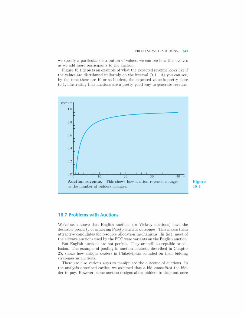
PROBLEMS WITH AUCTIONS 343
we specify a particular distribution of values, we can see how this evolvesas we add more participants to the auction.Figure 18.1 depicts an example of what the expected revenue looks like if
the values are distributed uniformly on the interval [0, 1]. As you can see,by the time there are 10 or so bidders, the expected value is pretty closeto 1, illustrating that auctions are a pretty good way to generate revenue.
0.0
0.2
0.4
0.6
0.8
1.0
0 10 20 30 40 n
REVENUE
Auction revenue. This shows how auction revenue changesas the number of bidders changes.
Figure18.1
18.7 Problems with Auctions
We’ve seen above that English auctions (or Vickrey auctions) have thedesirable property of achieving Pareto efficient outcomes. This makes themattractive candidates for resource allocation mechanisms. In fact, most ofthe airwave auctions used by the FCC were variants on the English auction.But English auctions are not perfect. They are still susceptible to col-
lusion. The example of pooling in auction markets, described in Chapter25, shows how antique dealers in Philadelphia colluded on their biddingstrategies in auctions.There are also various ways to manipulate the outcome of auctions. In
the analysis described earlier, we assumed that a bid committed the bid-der to pay. However, some auction designs allow bidders to drop out once
344 AUCTIONS (Ch. 18)
the winning bids are revealed. Such an option allows for manipulation.For example, in 1993 the Australian government auctioned off licenses forsatellite-television services using a standard sealed-bid auction. The win-ning bid for one of the licenses, A$212 million, was made by a companycalled Ucom. Once the government announced Ucom had won, they pro-ceeded to default on their bid, leaving the government to award the licenseto the second-highest bidder—which was also Ucom! They defaulted onthis bid as well; four months later, after several more defaults, they paidA$117 million for the license, which was A$95 million less than their initialwinning bid! The license ended up being awarded to the highest bidder atthe second-highest price—but the poorly designed auction caused at leasta year delay in bringing pay-TV to Australia.5
EXAMPLE: Taking Bids Off the Wall
One common method for manipulating auctions is for the seller to takefictitious bids, a practice known as “taking bids off the wall.” Such manip-ulation has found its way to online auctions as well, even where no wallsare involved.According to a recent news story,6 a New York jeweler sold large quanti-
ties of diamonds, gold, and platinum jewelry online. Though the items wereoffered on eBay with no reserve price, the seller distributed spreadsheetsto his employees which instructed them to place bids in order to increasethe final sales price. According to the lawsuit, the employees placed over232,000 bids in a one-year period, inflating the selling prices by 20% onaverage.When confronted with the evidence, the jeweler agreed to pay a $400,000
fine to settle the civil fraud complaint.
18.8 The Winner’s Curse
We turn now to the examination of common-value auctions, where thegood that is being awarded has the same value to all bidders. However, eachof the bidders may have different estimates of that value. To emphasizethis, let us write the (estimated) value of bidder i as v + εi where v is the
5 See John McMillan, “Selling Spectrum Rights,” Journal of Economic Perspectives,8(3), 145–152, for details of this story and how its lessons were incorporated into thedesign of the U.S. spectrum auction. This article also describes the New Zealandexample mentioned earlier.
6 Barnaby J. Feder, “Jeweler to Pay $400,000 in Online Auction Fraud Settlement,”New York Times, June 9, 2007.
STABLE MARRIAGE PROBLEM 345
true, common value and εi is the “error term” associated with bidder i’sestimate.
Let’s examine a sealed-bid auction in this framework. What bid shouldbidder i place? To develop some intuition, let’s see what happens if eachbidder bids their estimated value. In this case, the person with the highestvalue of εi, εmax, gets the good. But as long as εmax > 0, this personis paying more than v, the true value of the good. This is the so-calledWinner’s Curse. If you win the auction, it is because you have overes-timated the value of the good being sold. In other words, you have wononly because you were too optimistic!
The optimal strategy in a common-value auction like this is to bid lessthan your estimated value—and the more bidders there are, the lower youwant your own bid to be. Think about it: if you are the highest bidderout of five bidders you may be overly optimistic, but if you are the highestbidder out of twenty bidders you must be super optimistic. The morebidders there are, the more humble you should be about your own estimatesof the “true value” of the good in question.
The Winner’s Curse seemed to be operating in the FCC’s May 1996spectrum auction for personal communications services. The largest bidderin that auction, NextWave Personal Communications Inc., bid $4.2 billionfor sixty-three licenses, winning them all. However, in January 1998 thecompany filed for Chapter Eleven bankruptcy protection, after finding itselfunable to pay its bills.
18.9 Stable Marriage Problem
There are many examples of two-sided matching models where con-sumers are matched up with each other. Men may be matched with womenby a dating service or matchmaker, students may be matched with colleges,pledges may be matched with sororities, interns matched with hospitals,and so on.
What are good algorithms for making such matches? Do “stable” out-comes always exist? Here we examine a simple mechanism for makingmatches that are stable in a precisely defined sense.
Let us suppose that there are n men and an equal number of women andwe need to match them up as dancing partners. Each woman can rankthe men according to her preferences and the same goes for the men. Forsimplicity, let us suppose that there are no ties in these rankings and thateveryone would prefer to dance than to sit on the sidelines.
What is a good way to arrange for dancing partners? One attractivecriterion is to find a way to produce a “stable” matching. The definitionof stable, in this context, is that there is no couple that would prefer eachother to their current partner. Said another way, if a man prefers another
346 AUCTIONS (Ch. 18)
woman to his current partner, that woman wouldn’t want him—she wouldprefer the partner she currently had.Does a stable matching always exist? If so, how can one be found?
The answer is that, contrary to the impression one would get from soapoperas and romance novels, there always are stable matchings and they arerelatively easy to construct.The most famous algorithm, known as the deferred acceptance algo-
rithm, goes like this.7
Step 1. Each man proposes to his most preferred woman.
Step 2. Each woman records the list of proposals she receives on her dancecard.
Step 3. After all men have proposed to their most-preferred choice, eachwoman (gently) rejects all of the suitors except for her most preferred.
Step 4. The rejected suitors propose to the next woman on their lists.
Step 5. Continue to step 2 or terminate the algorithm when every womanhas received an offer.
This algorithm always produce a stable matching. Suppose, to the con-trary, that there is some man that prefers another woman to his presentpartner. Then he would have invited her to dance before his current part-ner. If she preferred him to her current partner, she would have rejectedher current partner earlier in the process.It turns out that this algorithm yields the best possible stable matching
for the men in the sense that each man prefers the outcome of this matchingprocess to any other stable matching. Of course, if we flipped the roles ofmen and women, we would find the woman-optimal stable matching.Though the example described is slightly frivolous, processes like the
deferred acceptance algorithm are used to match students to schools inBoston and New York, residents to hospitals nationwide, and even organdonors to recipients.
18.10 Mechanism Design
Auctions and the two-sided matching model that we have discussed in thischapter are examples of economic mechanisms. The idea of an economic
7 Gale, David, and Lloyd Shapley [1962], “College Admissions and the Stability ofMarriage,” American Mathematical Monthly, 69, 9-15.
MECHANISM DESIGN 347
mechanism is to define a “game” or “market” that will yield some desiredoutcome.For example, one might want to design a mechanism to sell a painting.
A natural mechanism here would be an auction. But even with an auction,there are many design choices. Should it be designed to maximize efficiency(i.e., to ensure that the painting goes to the person who values it mosthighly) or should it be designed to maximize expected revenue for theseller, even if there is a risk that the painting may not be sold?We’ve seen earlier that there are several different types of auctions, each
with advantages and disadvantages. Which one is best in a particularcircumstance?Mechanism design is essentially the inverse of game theory. With game
theory, we are given a description of the rules of the game and want todetermine what the outcome will be. With mechanism design, we aregiven a description of the outcome that we want to reach and try to designa game that will reach it.8
Mechanism design is not limited to auctions or matching problems. Italso includes voting mechanisms and public goodsmechanisms, such asthose described in Chapter 37, or externality mechanisms, such as thosedescribed in Chapter 35.In a general mechanism, we think of a number of agents (i.e., consumers
or firms) who each have some private information. In the case of an auction,this private information might be their value for the item being auctioned.In a problem involving firms, the private information might be their costfunctions.The agents report some message about their private information to the
“center,” which we might think of as an auctioneer. The center examinesthe messages and reports some outcome: who receives the item in question,what output firms should produce, how much various parties have to payor be paid, and so on.The major design decisions are 1) what sort of messages should be sent
to the center and 2) what rule the center should use to determine theoutcome. The constraints on the problem are the usual sort of resourceconstraints (i.e., there is only one item to be sold) and the constraints thatthe individuals will act in their own self-interest. This latter constraint isknown as the incentive compatibility constraint.
There may be other constraints as well. For example, we may want theagents to participate voluntarily in the mechanism, which would requirethat they get at least as high a payoff from participating as not participat-ing. We will ignore this constraint for simplicity.To get a flavor of what mechanism design looks like, let us consider
a simple problem of awarding an indivisible good to one of two different
8 The 2007 Nobel Prize in Economics was awarded to Leo Hurwicz, Roger Myerson,and Eric Maskin for their contributions to economic mechanism design.
348 AUCTIONS (Ch. 18)
agents. Let (x1, x2) = (1, 0) if agent 1 gets the good and (x1, x2) = (0, 1)if agent 2 gets the good. Let p be the price paid for the good.
We suppose that the message that each agent sends to the center is justa reported value for the good. This is known as a direct revelationmechanism. The center will then award the good to the agent with thehighest reported value and charge that agent some price p.
What are the constraints on p? Suppose agent 1 has the highest value.Then his message to the center should be such that the payoff he gets inresponse to that message is at least as large as the payoff he would get ifhe sent the same message as agent 2 (who gets a zero payoff). This says
v1 − p ≥ 0.
By the same token, agent 2 must get at least as large a payoff from hismessage as he would get if he sent the message sent by agent 1 (whichresulted in agent 1 getting the good). This says
0 ≥ v2 − p.
Putting these two conditions together, we have v1 ≥ p ≥ v2, which saysthat the price charged by the center must lie between the highest andsecond-highest value.In order to determine which price the center must charge, we need to
consider its objects and its information. If the center believes that the v1can be arbitrarily close to v2 and it always wants to award the item to thehighest bidder, then it has to set a price of v2.
This is just the Vickrey auction described earlier, in which each partysubmits a bid and the item is awarded to the highest bidder at the second-highest bid. This is clearly an attractive mechanism for this particularproblem.
Summary
1. Auctions have been used for thousands of years to sell things.
2. If each bidder’s value is independent of the other bidders, the auctionis said to be a private-value auction. If the value of the item being sold isessentially the same for everyone, the auction is said to be a common-valueauction.
3. Common auction forms are the English auction, the Dutch auction, thesealed-bid auction, and the Vickrey auction.
4. English auctions and Vickrey auctions have the desirable property thattheir outcomes are Pareto efficient.

REVIEW QUESTIONS 349
5. Profit-maximizing auctions typically require a strategic choice of thereservation price.
6. Despite their advantages as market mechanisms, auctions are vulnerableto collusion and other forms of strategic behavior.
REVIEW QUESTIONS
1. Consider an auction of antique quilts to collectors. Is this a private-valueor a common-value auction?
2. Suppose that there are only two bidders with values of $8 and $10 foran item with a bid increment of $1. What should the reservation price bein a profit-maximizing English auction?
3. Suppose that we have two copies of Intermediate Microeconomics to sellto three (enthusiastic) students. How can we use a sealed-bid auction thatwill guarantee that the bidders with the two highest values get the books?
4. Consider the Ucom example in the text. Was the auction design efficient?Did it maximize profits?
5. A game theorist fills a jar with pennies and auctions it off on the first dayof class using an English auction. Is this a private-value or a common-valueauction? Do you think the winning bidder usually makes a profit?

CHAPTER 19
TECHNOLOGY
In this chapter we begin our study of firm behavior. The first thing to do isto examine the constraints on a firm’s behavior. When a firm makes choicesit faces many constraints. These constraints are imposed by its customers,by its competitors, and by nature. In this chapter we’re going to considerthe latter source of constraints: nature. Nature imposes the constraint thatthere are only certain feasible ways to produce outputs from inputs: thereare only certain kinds of technological choices that are possible. Here wewill study how economists describe these technological constraints.If you understand consumer theory, production theory will be very easy
since the same tools are used. In fact, production theory is much simplerthan consumption theory because the output of a production process isgenerally observable, whereas the “output” of consumption (utility) is notdirectly observable.
19.1 Inputs and Outputs
Inputs to production are called factors of production. Factors of produc-tion are often classified into broad categories such as land, labor, capital,
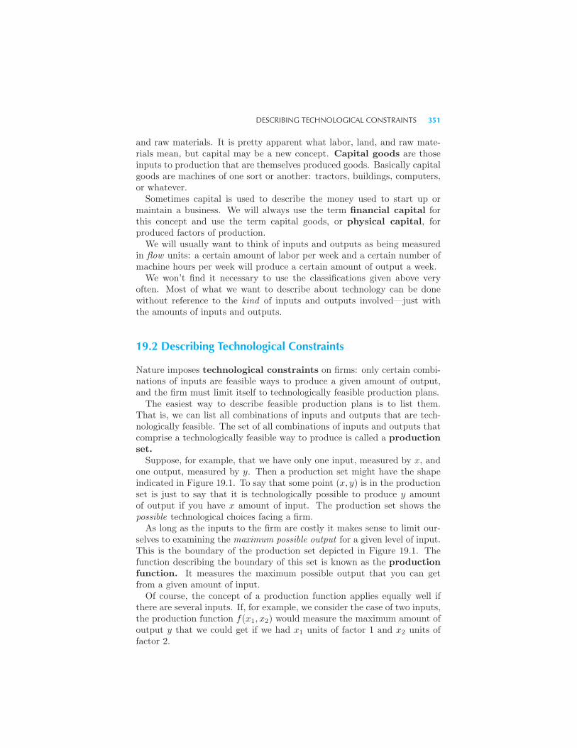
DESCRIBING TECHNOLOGICAL CONSTRAINTS 351
and raw materials. It is pretty apparent what labor, land, and raw mate-rials mean, but capital may be a new concept. Capital goods are thoseinputs to production that are themselves produced goods. Basically capitalgoods are machines of one sort or another: tractors, buildings, computers,or whatever.Sometimes capital is used to describe the money used to start up or
maintain a business. We will always use the term financial capital forthis concept and use the term capital goods, or physical capital, forproduced factors of production.We will usually want to think of inputs and outputs as being measured
in flow units: a certain amount of labor per week and a certain number ofmachine hours per week will produce a certain amount of output a week.We won’t find it necessary to use the classifications given above very
often. Most of what we want to describe about technology can be donewithout reference to the kind of inputs and outputs involved—just withthe amounts of inputs and outputs.
19.2 Describing Technological Constraints
Nature imposes technological constraints on firms: only certain combi-nations of inputs are feasible ways to produce a given amount of output,and the firm must limit itself to technologically feasible production plans.The easiest way to describe feasible production plans is to list them.
That is, we can list all combinations of inputs and outputs that are tech-nologically feasible. The set of all combinations of inputs and outputs thatcomprise a technologically feasible way to produce is called a productionset.Suppose, for example, that we have only one input, measured by x, and
one output, measured by y. Then a production set might have the shapeindicated in Figure 19.1. To say that some point (x, y) is in the productionset is just to say that it is technologically possible to produce y amountof output if you have x amount of input. The production set shows thepossible technological choices facing a firm.As long as the inputs to the firm are costly it makes sense to limit our-
selves to examining the maximum possible output for a given level of input.This is the boundary of the production set depicted in Figure 19.1. Thefunction describing the boundary of this set is known as the productionfunction. It measures the maximum possible output that you can getfrom a given amount of input.Of course, the concept of a production function applies equally well if
there are several inputs. If, for example, we consider the case of two inputs,the production function f(x1, x2) would measure the maximum amount ofoutput y that we could get if we had x1 units of factor 1 and x2 units offactor 2.
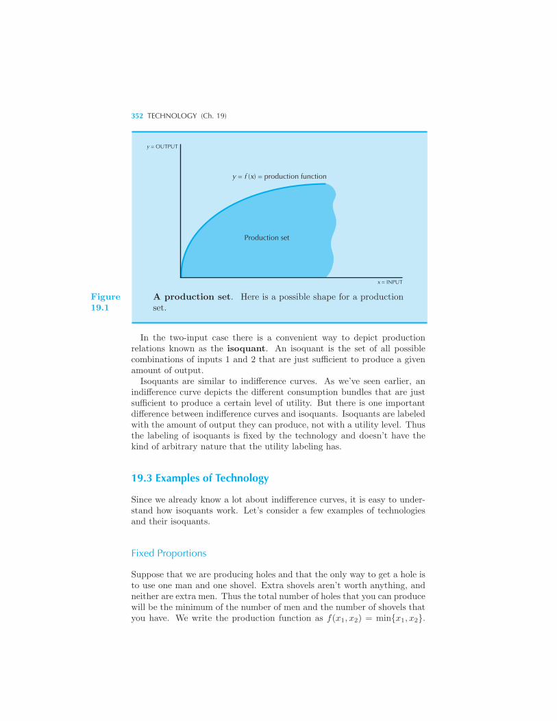
352 TECHNOLOGY (Ch. 19)
y = OUTPUT
Production set
y = f (x) = production function
x = INPUT
Figure19.1
A production set. Here is a possible shape for a productionset.
In the two-input case there is a convenient way to depict productionrelations known as the isoquant. An isoquant is the set of all possiblecombinations of inputs 1 and 2 that are just sufficient to produce a givenamount of output.Isoquants are similar to indifference curves. As we’ve seen earlier, an
indifference curve depicts the different consumption bundles that are justsufficient to produce a certain level of utility. But there is one importantdifference between indifference curves and isoquants. Isoquants are labeledwith the amount of output they can produce, not with a utility level. Thusthe labeling of isoquants is fixed by the technology and doesn’t have thekind of arbitrary nature that the utility labeling has.
19.3 Examples of Technology
Since we already know a lot about indifference curves, it is easy to under-stand how isoquants work. Let’s consider a few examples of technologiesand their isoquants.
Fixed Proportions
Suppose that we are producing holes and that the only way to get a hole isto use one man and one shovel. Extra shovels aren’t worth anything, andneither are extra men. Thus the total number of holes that you can producewill be the minimum of the number of men and the number of shovels thatyou have. We write the production function as f(x1, x2) = min{x1, x2}.
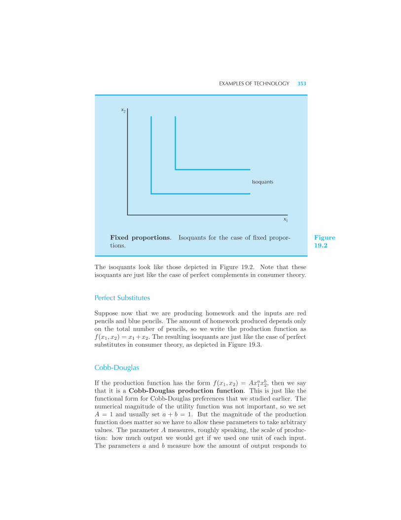
EXAMPLES OF TECHNOLOGY 353
Isoquants
x1
x2
Fixed proportions. Isoquants for the case of fixed propor-tions.
Figure19.2
The isoquants look like those depicted in Figure 19.2. Note that theseisoquants are just like the case of perfect complements in consumer theory.
Perfect Substitutes
Suppose now that we are producing homework and the inputs are redpencils and blue pencils. The amount of homework produced depends onlyon the total number of pencils, so we write the production function asf(x1, x2) = x1+x2. The resulting isoquants are just like the case of perfectsubstitutes in consumer theory, as depicted in Figure 19.3.
Cobb-Douglas
If the production function has the form f(x1, x2) = Axa1x
b2, then we say
that it is a Cobb-Douglas production function. This is just like thefunctional form for Cobb-Douglas preferences that we studied earlier. Thenumerical magnitude of the utility function was not important, so we setA = 1 and usually set a + b = 1. But the magnitude of the productionfunction does matter so we have to allow these parameters to take arbitraryvalues. The parameter A measures, roughly speaking, the scale of produc-tion: how much output we would get if we used one unit of each input.The parameters a and b measure how the amount of output responds to
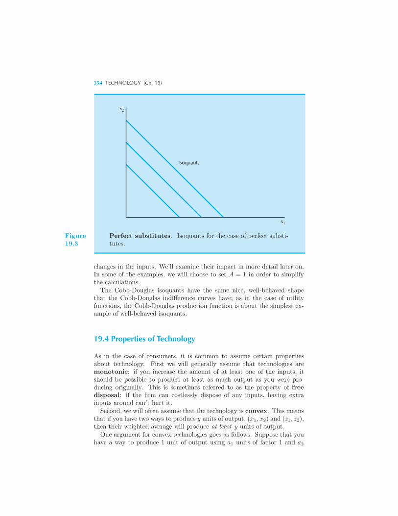
354 TECHNOLOGY (Ch. 19)
x2
Isoquants
x1
Figure19.3
Perfect substitutes. Isoquants for the case of perfect substi-tutes.
changes in the inputs. We’ll examine their impact in more detail later on.In some of the examples, we will choose to set A = 1 in order to simplifythe calculations.The Cobb-Douglas isoquants have the same nice, well-behaved shape
that the Cobb-Douglas indifference curves have; as in the case of utilityfunctions, the Cobb-Douglas production function is about the simplest ex-ample of well-behaved isoquants.
19.4 Properties of Technology
As in the case of consumers, it is common to assume certain propertiesabout technology. First we will generally assume that technologies aremonotonic: if you increase the amount of at least one of the inputs, itshould be possible to produce at least as much output as you were pro-ducing originally. This is sometimes referred to as the property of freedisposal: if the firm can costlessly dispose of any inputs, having extrainputs around can’t hurt it.Second, we will often assume that the technology is convex. This means
that if you have two ways to produce y units of output, (x1, x2) and (z1, z2),then their weighted average will produce at least y units of output.One argument for convex technologies goes as follows. Suppose that you
have a way to produce 1 unit of output using a1 units of factor 1 and a2
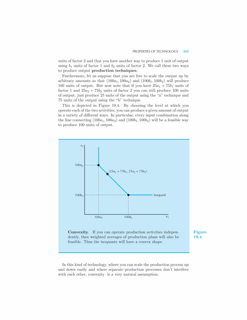
PROPERTIES OF TECHNOLOGY 355
units of factor 2 and that you have another way to produce 1 unit of outputusing b1 units of factor 1 and b2 units of factor 2. We call these two waysto produce output production techniques.
Furthermore, let us suppose that you are free to scale the output up byarbitrary amounts so that (100a1, 100a2) and (100b1, 100b2) will produce100 units of output. But now note that if you have 25a1 + 75b1 units offactor 1 and 25a2 + 75b2 units of factor 2 you can still produce 100 unitsof output: just produce 25 units of the output using the “a” technique and75 units of the output using the “b” technique.
This is depicted in Figure 19.4. By choosing the level at which youoperate each of the two activities, you can produce a given amount of outputin a variety of different ways. In particular, every input combination alongthe line connecting (100a1, 100a2) and (100b1, 100b2) will be a feasible wayto produce 100 units of output.
100a2
100b2
x2
100b1100a1
Isoquant
(25a1 + 75b1, 25a2 + 75b2)
x1
Convexity. If you can operate production activities indepen-dently, then weighted averages of production plans will also befeasible. Thus the isoquants will have a convex shape.
Figure19.4
In this kind of technology, where you can scale the production process upand down easily and where separate production processes don’t interferewith each other, convexity is a very natural assumption.
356 TECHNOLOGY (Ch. 19)
19.5 The Marginal Product
Suppose that we are operating at some point, (x1, x2), and that we considerusing a little bit more of factor 1 while keeping factor 2 fixed at the levelx2. How much more output will we get per additional unit of factor 1? Wehave to look at the change in output per unit change of factor 1:
Δy
Δx1=
f(x1 +Δx1, x2)− f(x1, x2)
Δx1.
We call this the marginal product of factor 1. The marginal productof factor 2 is defined in a similar way, and we denote them by MP1(x1, x2)and MP2(x1, x2), respectively.Sometimes we will be a bit sloppy about the concept of marginal product
and describe it as the extra output we get from having “one” more unit offactor 1. As long as “one” is small relative to the total amount of factor 1that we are using, this will be satisfactory. But we should remember thata marginal product is a rate: the extra amount of output per unit of extrainput.The concept of marginal product is just like the concept of marginal
utility that we described in our discussion of consumer theory, except forthe ordinal nature of utility. Here, we are discussing physical output: themarginal product of a factor is a specific number, which can, in principle,be observed.
19.6 The Technical Rate of Substitution
Suppose that we are operating at some point (x1, x2) and that we considergiving up a little bit of factor 1 and using just enough more of factor 2 toproduce the same amount of output y. How much extra of factor 2, Δx2,do we need if we are going to give up a little bit of factor 1, Δx1? Thisis just the slope of the isoquant; we refer to it as the technical rate ofsubstitution (TRS), and denote it by TRS(x1, x2).The technical rate of substitution measures the tradeoff between two
inputs in production. It measures the rate at which the firm will have tosubstitute one input for another in order to keep output constant.To derive a formula for the TRS, we can use the same idea that we used
to determine the slope of the indifference curve. Consider a change in ouruse of factors 1 and 2 that keeps output fixed. Then we have
Δy = MP1(x1, x2)Δx1 +MP2(x1, x2)Δx2 = 0,
which we can solve to get
TRS(x1, x2) =Δx2
Δx1= −MP1(x1, x2)
MP2(x1, x2).
Note the similarity with the definition of the marginal rate of substitution.
DIMINISHING TECHNICAL RATE OF SUBSTITUTION 357
19.7 Diminishing Marginal Product
Suppose that we have certain amounts of factors 1 and 2 and we consideradding more of factor 1 while holding factor 2 fixed at a given level. Whatmight happen to the marginal product of factor 1?As long as we have a monotonic technology, we know that the total
output will go up as we increase the amount of factor 1. But it is naturalto expect that it will go up at a decreasing rate. Let’s consider a specificexample, the case of farming.One man on one acre of land might produce 100 bushels of corn. If we
add another man and keep the same amount of land, we might get 200bushels of corn, so in this case the marginal product of an extra workeris 100. Now keep adding workers to this acre of land. Each worker mayproduce more output, but eventually the extra amount of corn producedby an extra worker will be less than 100 bushels. After 4 or 5 people areadded the additional output per worker will drop to 90, 80, 70 . . . or evenfewer bushels of corn. If we get hundreds of workers crowded together onthis one acre of land, an extra worker may even cause output to go down!As in the making of broth, extra cooks can make things worse.Thus we would typically expect that the marginal product of a factor
will diminish as we get more and more of that factor. This is called thelaw of diminishing marginal product. It isn’t really a “law”; it’s justa common feature of most kinds of production processes.It is important to emphasize that the law of diminishing marginal prod-
uct applies only when all other inputs are being held fixed. In the farmingexample, we considered changing only the labor input, holding the landand raw materials fixed.
19.8 Diminishing Technical Rate of Substitution
Another closely related assumption about technology is that of diminish-ing technical rate of substitution. This says that as we increase theamount of factor 1, and adjust factor 2 so as to stay on the same isoquant,the technical rate of substitution declines. Roughly speaking, the assump-tion of diminishing TRS means that the slope of an isoquant must decreasein absolute value as we move along the isoquant in the direction of increas-ing x1, and it must increase as we move in the direction of increasing x2.This means that the isoquants will have the same sort of convex shape thatwell-behaved indifference curves have.The assumptions of a diminishing technical rate of substitution and di-
minishing marginal product are closely related but are not exactly thesame. Diminishing marginal product is an assumption about how the mar-ginal product changes as we increase the amount of one factor, holding the
358 TECHNOLOGY (Ch. 19)
other factor fixed. Diminishing TRS is about how the ratio of the marginalproducts—the slope of the isoquant—changes as we increase the amountof one factor and reduce the amount of the other factor so as to stay on thesame isoquant.
19.9 The Long Run and the Short Run
Let us return now to the original idea of a technology as being just a listof the feasible production plans. We may want to distinguish between theproduction plans that are immediately feasible and those that are eventuallyfeasible.In the short run, there will be some factors of production that are fixed
at predetermined levels. Our farmer described above might only considerproduction plans that involve a fixed amount of land, if that is all he hasaccess to. It may be true that if he had more land, he could produce morecorn, but in the short run he is stuck with the amount of land that he has.On the other hand, in the long run the farmer is free to purchase more
land, or to sell some of the land he now owns. He can adjust the level ofthe land input so as to maximize his profits.The economist’s distinction between the long run and the short run is
this: in the short run there is at least one factor of production that is fixed:a fixed amount of land, a fixed plant size, a fixed number of machines, orwhatever. In the long run, all the factors of production can be varied.
There is no specific time interval implied here. What is the long run andwhat is the short run depends on what kinds of choices we are examining.In the short run at least some factors are fixed at given levels, but in thelong run the amount used of these factors can be changed.Let’s suppose that factor 2, say, is fixed at x2 in the short run. Then the
relevant production function for the short run is f(x1, x2). We can plot thefunctional relation between output and x1 in a diagram like Figure 19.5.Note that we have drawn the short-run production function as getting
flatter and flatter as the amount of factor 1 increases. This is just the lawof diminishing marginal product in action again. Of course, it can easilyhappen that there is an initial region of increasing marginal returns wherethe marginal product of factor 1 increases as we add more of it. In the caseof the farmer adding labor, it might be that the first few workers addedincrease output more and more because they would be able to divide upjobs efficiently, and so on. But given the fixed amount of land, eventuallythe marginal product of labor will decline.
19.10 Returns to Scale
Now let’s consider a different kind of experiment. Instead of increasing theamount of one input while holding the other input fixed, let’s increase the
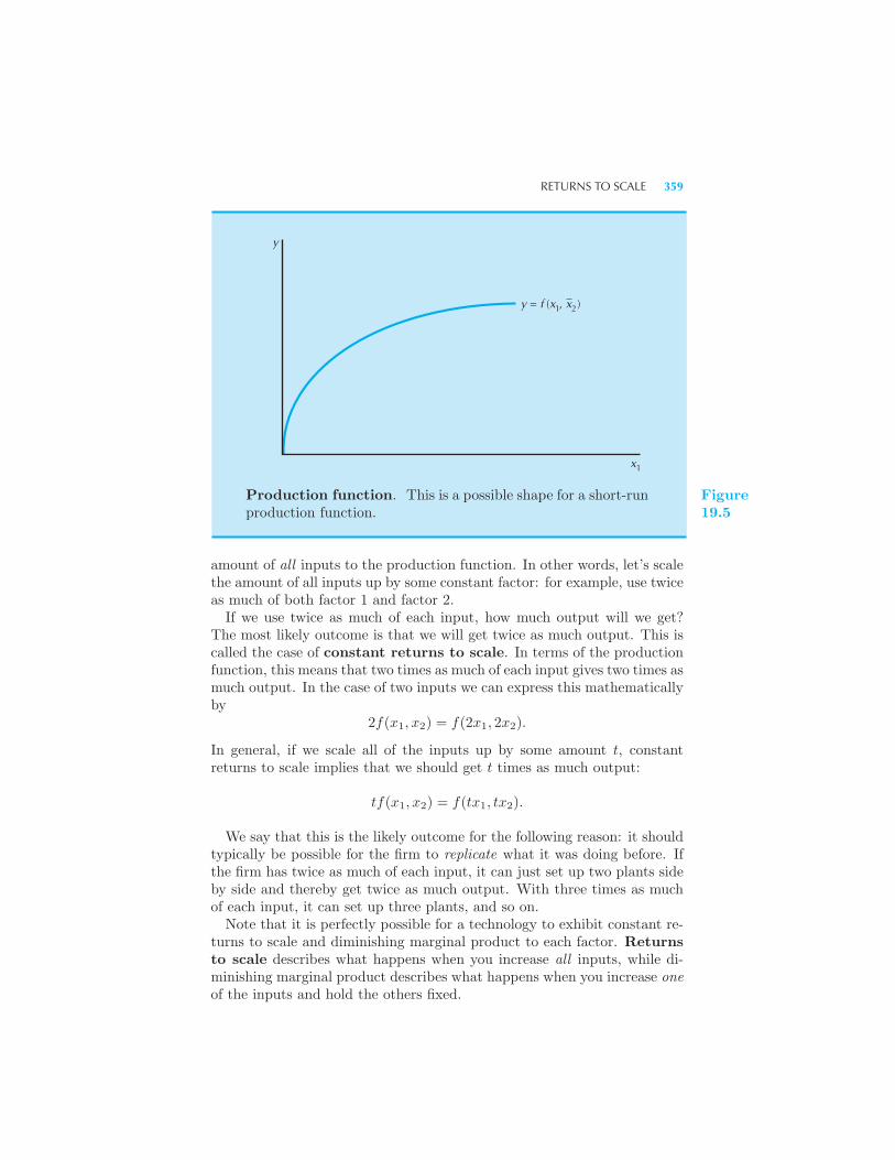
RETURNS TO SCALE 359
y
y = f (x , x )
x1
1 2
Production function. This is a possible shape for a short-runproduction function.
Figure19.5
amount of all inputs to the production function. In other words, let’s scalethe amount of all inputs up by some constant factor: for example, use twiceas much of both factor 1 and factor 2.If we use twice as much of each input, how much output will we get?
The most likely outcome is that we will get twice as much output. This iscalled the case of constant returns to scale. In terms of the productionfunction, this means that two times as much of each input gives two times asmuch output. In the case of two inputs we can express this mathematicallyby
2f(x1, x2) = f(2x1, 2x2).
In general, if we scale all of the inputs up by some amount t, constantreturns to scale implies that we should get t times as much output:
tf(x1, x2) = f(tx1, tx2).
We say that this is the likely outcome for the following reason: it shouldtypically be possible for the firm to replicate what it was doing before. Ifthe firm has twice as much of each input, it can just set up two plants sideby side and thereby get twice as much output. With three times as muchof each input, it can set up three plants, and so on.Note that it is perfectly possible for a technology to exhibit constant re-
turns to scale and diminishing marginal product to each factor. Returnsto scale describes what happens when you increase all inputs, while di-minishing marginal product describes what happens when you increase oneof the inputs and hold the others fixed.
360 TECHNOLOGY (Ch. 19)
Constant returns to scale is the most “natural” case because of the repli-cation argument, but that isn’t to say that other things might not happen.For example, it could happen that if we scale up both inputs by some fac-tor t, we get more than t times as much output. This is called the case ofincreasing returns to scale. Mathematically, increasing returns to scalemeans that
f(tx1, tx2) > tf(x1, x2).
for all t > 1.What would be an example of a technology that had increasing returns
to scale? One nice example is that of an oil pipeline. If we double thediameter of a pipe, we use twice as much materials, but the cross sectionof the pipe goes up by a factor of 4. Thus we will likely be able to pumpmore than twice as much oil through it.(Of course, we can’t push this example too far. If we keep doubling the
diameter of the pipe, it will eventually collapse of its own weight. Increasingreturns to scale usually just applies over some range of output.)The other case to consider is that of decreasing returns to scale,
where
f(tx1, tx2) < tf(x1, x2)
for all t > 1.This case is somewhat peculiar. If we get less than twice as much output
from having twice as much of each input, we must be doing somethingwrong. After all, we could just replicate what we were doing before!The usual way in which diminishing returns to scale arises is because we
forgot to account for some input. If we have twice as much of every inputbut one, we won’t be able to exactly replicate what we were doing before, sothere is no reason that we have to get twice as much output. Diminishingreturns to scale is really a short-run phenomenon, with something beingheld fixed.Of course, a technology can exhibit different kinds of returns to scale
at different levels of production. It may well happen that for low levelsof production, the technology exhibits increasing returns to scale—as youscale all the inputs by some small amount t, the output increases by morethan t. Later on, for larger levels of output, increasing scale by t may justincrease output by the same factor t.
EXAMPLE: Datacenters
Datacenters are large buildings that house thousands of computers usedto perform tasks such as serving web pages. Internet companies such asGoogle, Yahoo, Microsoft, Amazon, and many others have built thousandsof datacenters around the world.
SUMMARY 361
A typical datacenter consists of hundreds of racks which hold computermotherboards that are similar to the motherboard in your desktop com-puter. Generally these systems are designed to be easily scalable so thatthe computational power of the data center can scale up or down just byadding or removing racks of computers.The replication argument implies that the production function for com-
puting services is effectively constant returns to scale: to double output,you simply double all inputs.
EXAMPLE: Copy Exactly!
Intel operates dozens of “fab plants” that fabricate, assemble, sort, and testadvanced computer chips. Chip fabrication is such a delicate process thatIntel found it difficult to manage quality in a heterogeneous environment.Even minor variations in plant design, such as cleaning procedures or thelength of cooling hoses, could have a large impact on the yield of the fabprocess.In order to manage these very subtle effects, Intel moved to its Copy
Exactly! process. According to Intel, the Copy Exactly directive is: “ev-erything which might affect the process, or how it is run, is to be copieddown to the finest detail, unless it is either physically impossible to do so,or there is an overwhelming competitive benefit to introducing a change.”This means that one Intel plant is very much like another, and deliber-
ately so. As the replication argument suggests, the easiest way to scale upproduction at Intel is to replicate current operating procedures as closelyas possible.
Summary
1. The technological constraints of the firm are described by the productionset, which depicts all the technologically feasible combinations of inputsand outputs, and by the production function, which gives the maximumamount of output associated with a given amount of the inputs.
2. Another way to describe the technological constraints facing a firm isthrough the use of isoquants—curves that indicate all the combinations ofinputs capable of producing a given level of output.
3. We generally assume that isoquants are convex and monotonic, just likewell–behaved preferences.
4. The marginal product measures the extra output per extra unit of aninput, holding all other inputs fixed. We typically assume that the marginalproduct of an input diminishes as we use more and more of that input.
362 TECHNOLOGY (Ch. 19)
5. The technical rate of substitution (TRS) measures the slope of an iso-quant. We generally assume that the TRS diminishes as we move out alongan isoquant—which is another way of saying that the isoquant has a convexshape.
6. In the short run some inputs are fixed, while in the long run all inputsare variable.
7. Returns to scale refers to the way that output changes as we changethe scale of production. If we scale all inputs up by some amount t andoutput goes up by the same factor, then we have constant returns to scale.If output scales up by more that t, we have increasing returns to scale; andif it scales up by less than t, we have decreasing returns to scale.
REVIEW QUESTIONS
1. Consider the production function f(x1, x2) = x21x
22. Does this exhibit
constant, increasing, or decreasing returns to scale?
2. Consider the production function f(x1, x2) = 4x121 x
132 . Does this exhibit
constant, increasing, or decreasing returns to scale?
3. The Cobb-Douglas production function is given by f(x1, x2) = Axa1x
b2.
It turns out that the type of returns to scale of this function will dependon the magnitude of a + b. Which values of a + b will be associated withthe different kinds of returns to scale?
4. The technical rate of substitution between factors x2 and x1 is −4. Ifyou desire to produce the same amount of output but cut your use of x1
by 3 units, how many more units of x2 will you need?
5. True or false? If the law of diminishing marginal product did not hold,the world’s food supply could be grown in a flowerpot.
6. In a production process is it possible to have decreasing marginal productin an input and yet increasing returns to scale?
CHAPTER 20
PROFITMAXIMIZATION
In the last chapter we discussed ways to describe the technological choicesfacing the firm. In this chapter we describe a model of how the firm choosesthe amount to produce and the method of production to employ. Themodel we will use is the model of profit maximization: the firm chooses aproduction plan so as to maximize its profits.In this chapter we will assume that the firm faces fixed prices for its in-
puts and outputs. We said earlier that economists call a market where theindividual producers take the prices as outside their control a competitivemarket. So in this chapter we want to study the profit-maximization prob-lem of a firm that faces competitive markets for the factors of productionit uses and the output goods it produces.
20.1 Profits
Profits are defined as revenues minus cost. Suppose that the firm producesn outputs (y1, . . . , yn) and uses m inputs (x1, . . . , xm). Let the prices of theoutput goods be (p1, . . . , pn) and the prices of the inputs be (w1, . . . , wm).
364 PROFIT MAXIMIZATION (Ch. 20)
The profits the firm receives, π, can be expressed as
π =n∑
i=1
piyi −m∑i=1
wixi.
The first term is revenue, and the second term is cost.
In the expression for cost we should be sure to include all of the factorsof production used by the firm, valued at their market price. Usually thisis pretty obvious, but in cases where the firm is owned and operated by thesame individual, it is possible to forget about some of the factors.
For example, if an individual works in his own firm, then his labor is aninput and it should be counted as part of the costs. His wage rate is simplythe market price of his labor—what he would be getting if he sold his laboron the open market. Similarly, if a farmer owns some land and uses it inhis production, that land should be valued at its market value for purposesof computing the economic costs.
We have seen that economic costs like these are often referred to as op-portunity costs. The name comes from the idea that if you are usingyour labor, for example, in one application, you forgo the opportunity ofemploying it elsewhere. Therefore those lost wages are part of the cost ofproduction. Similarly with the land example: the farmer has the oppor-tunity of renting his land to someone else, but he chooses to forgo thatrental income in favor of renting it to himself. The lost rents are part ofthe opportunity cost of his production.
The economic definition of profit requires that we value all inputs andoutputs at their opportunity cost. Profits as determined by accountants donot necessarily accurately measure economic profits, as they typically usehistorical costs—what a factor was purchased for originally—rather thaneconomic costs—what a factor would cost if purchased now. There aremany variations on the use of the term “profit,” but we will always stickto the economic definition.
Another confusion that sometimes arises is due to getting time scalesmixed up. We usually think of the factor inputs as being measured interms of flows. So many labor hours per week and so many machine hoursper week will produce so much output per week. Then the factor prices willbe measured in units appropriate for the purchase of such flows. Wages arenaturally expressed in terms of dollars per hour. The analog for machineswould be the rental rate—the rate at which you can rent a machine forthe given time period.
In many cases there isn’t a very well-developed market for the rental ofmachines, since firms will typically buy their capital equipment. In thiscase, we have to compute the implicit rental rate by seeing how much itwould cost to buy a machine at the beginning of the period and sell it atthe end of the period.
PROFITS AND STOCK MARKET VALUE 365
20.2 The Organization of Firms
In a capitalist economy, firms are owned by individuals. Firms are onlylegal entities; ultimately it is the owners of firms who are responsible forthe behavior of the firm, and it is the owners who reap the rewards or paythe costs of that behavior.Generally speaking, firms can be organized as proprietorships, partner-
ships, or corporations. A proprietorship is a firm that is owned by asingle individual. A partnership is owned by two or more individuals. Acorporation is usually owned by several individuals as well, but under thelaw has an existence separate from that of its owners. Thus a partnershipwill last only as long as both partners are alive and agree to maintain itsexistence. A corporation can last longer than the lifetimes of any of itsowners. For this reason, most large firms are organized as corporations.The owners of each of these different types of firms may have different
goals with respect to managing the operation of the firm. In a proprietor-ship or a partnership the owners of the firm usually take a direct role inactually managing the day-to-day operations of the firm, so they are in aposition to carry out whatever objectives they have in operating the firm.Typically, the owners would be interested in maximizing the profits of theirfirm, but, if they have nonprofit goals, they can certainly indulge in thesegoals instead.In a corporation, the owners of the corporation are often distinct from
the managers of the corporation. Thus there is a separation of ownershipand control. The owners of the corporation must define an objective forthe managers to follow in their running of the firm, and then do theirbest to see that they actually pursue the goals the owners have in mind.Again, profit maximization is a common goal. As we’ll see below, this goal,properly interpreted, is likely to lead the managers of the firm to chooseactions that are in the interests of the owners of the firm.
20.3 Profits and Stock Market Value
Often the production process that a firm uses goes on for many periods.Inputs put in place at time t pay off with a whole flow of services at latertimes. For example, a factory building erected by a firm could last for 50or 100 years. In this case an input at one point in time helps to produceoutput at other times in the future.In this case we have to value a flow of costs and a flow of revenues over
time. As we’ve seen in Chapter 10, the appropriate way to do this is touse the concept of present value. When people can borrow and lend infinancial markets, the interest rate can be used to define a natural priceof consumption at different times. Firms have access to the same sorts of
366 PROFIT MAXIMIZATION (Ch. 20)
financial markets, and the interest rate can be used to value investmentdecisions in exactly the same way.Consider a world of perfect certainty where a firm’s flow of future profits
is publicly known. Then the present value of those profits would be thepresent value of the firm. It would be how much someone would bewilling to pay to purchase the firm.As we indicated above, most large firms are organized as corporations,
which means that they are jointly owned by a number of individuals. Thecorporation issues stock certificates to represent ownership of shares in thecorporation. At certain times the corporation issues dividends on theseshares, which represent a share of the profits of the firm. The shares ofownership in the corporation are bought and sold in the stock market.The price of a share represents the present value of the stream of dividendsthat people expect to receive from the corporation. The total stock marketvalue of a firm represents the present value of the stream of profits that thefirm is expected to generate. Thus the objective of the firm—maximizingthe present value of the stream of profits the firm generates—could alsobe described as the goal of maximizing stock market value. In a world ofcertainty, these two goals are the same thing.The owners of the firm will generally want the firm to choose production
plans that maximize the stock market value of the firm, since that will makethe value of the shares they hold as large as possible. We saw in Chapter10 that whatever an individual’s tastes for consumption at different times,he or she will always prefer an endowment with a higher present value toone with a lower present value. By maximizing stock market value, a firmmakes its shareholders’ budget sets as large as possible, and thereby actsin the best interests of all of its shareholders.If there is uncertainty about a firm’s stream of profits, then instructing
managers to maximize profits has no meaning. Should they maximize ex-pected profits? Should they maximize the expected utility of profits? Whatattitude toward risky investments should the managers have? It is diffi-cult to assign a meaning to profit maximization when there is uncertaintypresent. However, in a world of uncertainty, maximizing stock market valuestill has meaning. If the managers of a firm attempt to make the value ofthe firm’s shares as large as possible then they make the firm’s owners—theshareholders—as well-off as possible. Thus maximizing stock market valuegives a well-defined objective function to the firm in nearly all economicenvironments.Despite these remarks about time and uncertainty, we will generally limit
ourselves to the examination of much simpler profit-maximization prob-lems, namely, those in which there is a single, certain output and a singleperiod of time. This simple story still generates significant insights andbuilds the proper intuition to study more general models of firm behavior.Most of the ideas that we will examine carry over in a natural way to thesemore general models.
THE BOUNDARIES OF THE FIRM 367
20.4 The Boundaries of the Firm
One question that constantly confronts managers of firms is whether to“make or buy.” That is, should a firm make something internally or buy itfrom an external supplier? The question is broader than it sounds, as it canrefer not only to physical goods, but also services of one sort or another.Indeed, in the broadest interpretation, “make or buy” applies to almostevery decision a firm makes.Should a company provide its own cafeteria? Janitorial services? Pho-
tocopying services? Travel assistance? Obviously, many factors enter intosuch decisions. One important consideration is size. A small mom-and-popvideo store with 12 employees is probably not going to provide a cafeteria.But it might outsource janitorial services, depending on cost, capabilities,and staffing.Even a large organization, which could easily afford to operate food ser-
vices, may or may not choose to do so, depending on availability of alter-natives. Employees of an organization located in a big city have access tomany places to eat; if the organization is located in a remote area, choicesmay be fewer.One critical issue is whether the goods or services in question are exter-
nally provided by a monopoly or by a competitive market. By and large,managers prefer to buy goods and services on a competitive market, if theyare available. The second-best choice is dealing with an internal monop-olist. The worse choice of all, in terms of price and quality of service, isdealing with an external monopolist.Think about photocopying services. The ideal situation is to have dozens
of competitive providers vying for your business; that way you will getcheap prices and high-quality service. If your school is large, or in an urbanarea, there may be many photocopying services vying for your business. Onthe other hand, small rural schools may have less choice and often higherprices.The same is true of businesses. A highly competitive environment gives
lots of choices to users. By comparison, an internal photocopying divisionmay be less attractive. Even if prices are low, the service could be sluggish.But the least attractive option is surely to have to submit to a singleexternal provider. An internal monopoly provider may have bad service,but at least the money stays inside the firm.As technology changes, what is typically inside the firm changes. Forty
years ago, firms managed many services themselves. Now they tend tooutsource as much as possible. Food service, photocopying service, andjanitorial services are often provided by external organizations that spe-cialize in such activities. Such specialization often allows these companiesto provide higher quality and less expensive services to the organizationsthat use their services.
368 PROFIT MAXIMIZATION (Ch. 20)
20.5 Fixed and Variable Factors
In a given time period, it may be very difficult to adjust some of the inputs.Typically a firm may have contractual obligations to employ certain inputsat certain levels. An example of this would be a lease on a building, wherethe firm is legally obligated to purchase a certain amount of space over theperiod under examination. We refer to a factor of production that is ina fixed amount for the firm as a fixed factor. If a factor can be used indifferent amounts, we refer to it as a variable factor.As we saw in Chapter 19, the short run is defined as that period of time
in which there are some fixed factors—factors that can only be used infixed amounts. In the long run, on the other hand, the firm is free to varyall of the factors of production: all factors are variable factors.There is no rigid boundary between the short run and the long run. The
exact time period involved depends on the problem under examination.The important thing is that some of the factors of production are fixed inthe short run and variable in the long run. Since all factors are variable inthe long run, a firm is always free to decide to use zero inputs and producezero output—that is, to go out of business. Thus the least profits a firmcan make in the long run are zero profits.In the short run, the firm is obligated to employ some factors, even if it
decides to produce zero output. Therefore it is perfectly possible that thefirm could make negative profits in the short run.
By definition, fixed factors are factors of production that must be paidfor even if the firm decides to produce zero output: if a firm has a long-term lease on a building, it must make its lease payments each periodwhether or not it decides to produce anything that period. But there isanother category of factors that only need to be paid for if the firm decidesto produce a positive amount of output. One example is electricity usedfor lighting. If the firm produces zero output, it doesn’t have to provideany lighting; but if it produces any positive amount of output, it has topurchase a fixed amount of electricity to use for lighting.Factors such as these are called quasi-fixed factors. They are factors of
production that must be used in a fixed amount, independent of the outputof the firm, as long as the output is positive. The distinction betweenfixed factors and quasi-fixed factors is sometimes useful in analyzing theeconomic behavior of the firm.
20.6 Short-Run Profit Maximization
Let’s consider the short-run profit-maximization problem when input 2 isfixed at some level x2. Let f(x1, x2) be the production function for thefirm, let p be the price of output, and let w1 and w2 be the prices of the
SHORT-RUN PROFIT MAXIMIZATION 369
two inputs. Then the profit-maximization problem facing the firm can bewritten as
maxx1
pf(x1, x2)− w1x1 − w2x2.
The condition for the optimal choice of factor 1 is not difficult to determine.If x∗
1 is the profit-maximizing choice of factor 1, then the output pricetimes the marginal product of factor 1 should equal the price of factor 1.In symbols,
pMP1(x∗1, x2) = w1.
In other words, the value of the marginal product of a factor should equalits price.
In order to understand this rule, think about the decision to employ alittle more of factor 1. As you add a little more of it, Δx1, you produceΔy = MP1Δx1 more output that is worth pMP1Δx1. But this marginaloutput costs w1Δx1 to produce. If the value of marginal product exceedsits cost, then profits can be increased by increasing input 1. If the valueof marginal product is less than its cost, then profits can be increased bydecreasing the level of input 1.If the profits of the firm are as large as possible, then profits should
not increase when we increase or decrease input 1. This means that at aprofit-maximizing choice of inputs and outputs, the value of the marginalproduct, pMP1(x
∗1, x2), should equal the factor price, w1.
We can derive the same condition graphically. Consider Figure 20.1. Thecurved line represents the production function holding factor 2 fixed at x2.Using y to denote the output of the firm, profits are given by
π = py − w1x1 − w2x2.
This expression can be solved for y to express output as a function of x1:
y =π
p+
w2
px2 +
w1
px1. (20.1)
This equation describes isoprofit lines. These are just all combinationsof the input goods and the output good that give a constant level of profit,π. As π varies we get a family of parallel straight lines each with a slope ofw1/p and each having a vertical intercept of π/p+w2x2/p, which measuresthe profits plus the fixed costs of the firm.The fixed costs are fixed, so the only thing that really varies as we move
from one isoprofit line to another is the level of profits. Thus higher levels ofprofit will be associated with isoprofit lines with higher vertical intercepts.The profit-maximization problem is then to find the point on the produc-
tion function that has the highest associated isoprofit line. Such a pointis illustrated in Figure 20.1. As usual it is characterized by a tangencycondition: the slope of the production function should equal the slope of
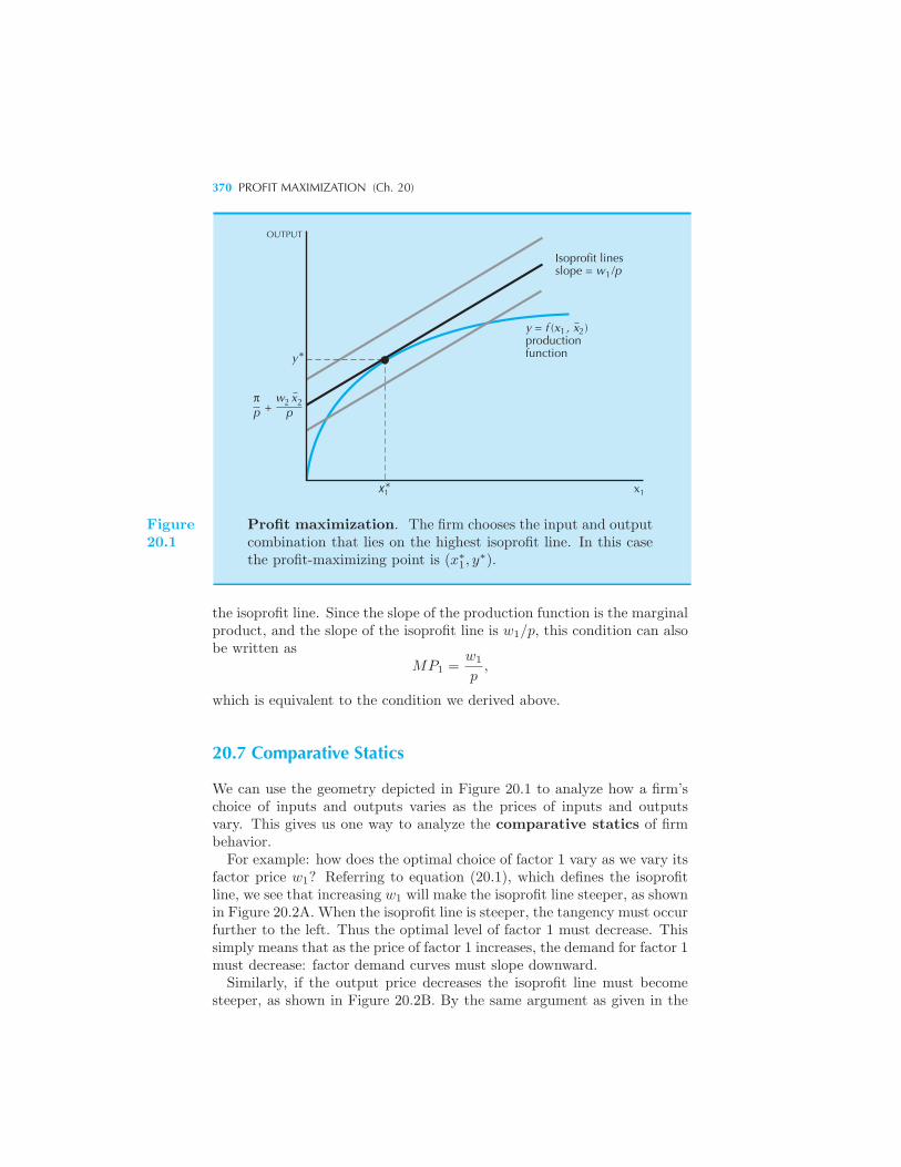
370 PROFIT MAXIMIZATION (Ch. 20)
OUTPUT
y*
x *1 1x
Isoprofit linesslope = w /p1
y = f (x , x )production function
1 2
πp +
w x2 2p
Figure20.1
Profit maximization. The firm chooses the input and outputcombination that lies on the highest isoprofit line. In this casethe profit-maximizing point is (x∗
1, y∗).
the isoprofit line. Since the slope of the production function is the marginalproduct, and the slope of the isoprofit line is w1/p, this condition can alsobe written as
MP1 =w1
p,
which is equivalent to the condition we derived above.
20.7 Comparative Statics
We can use the geometry depicted in Figure 20.1 to analyze how a firm’schoice of inputs and outputs varies as the prices of inputs and outputsvary. This gives us one way to analyze the comparative statics of firmbehavior.For example: how does the optimal choice of factor 1 vary as we vary its
factor price w1? Referring to equation (20.1), which defines the isoprofitline, we see that increasing w1 will make the isoprofit line steeper, as shownin Figure 20.2A. When the isoprofit line is steeper, the tangency must occurfurther to the left. Thus the optimal level of factor 1 must decrease. Thissimply means that as the price of factor 1 increases, the demand for factor 1must decrease: factor demand curves must slope downward.Similarly, if the output price decreases the isoprofit line must become
steeper, as shown in Figure 20.2B. By the same argument as given in the
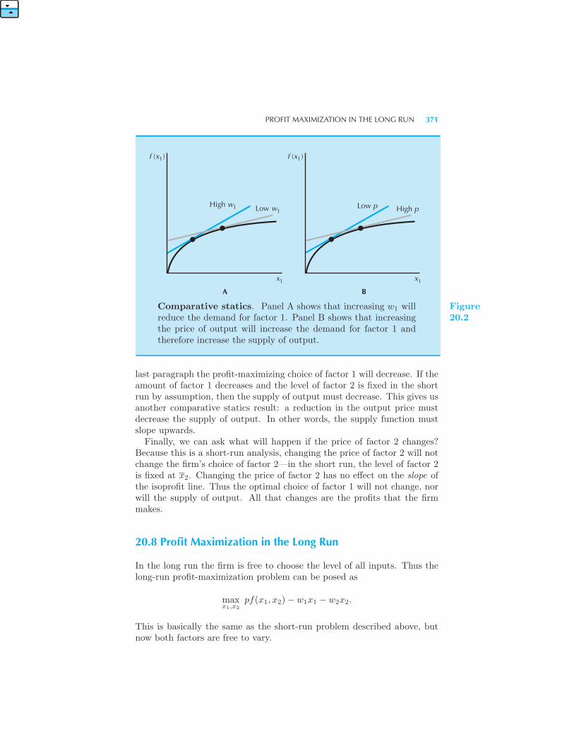
PROFIT MAXIMIZATION IN THE LONG RUN 371
f (x )1
High wHigh pLow pLow w
x
BA1
11
f (x )1
x1
Comparative statics. Panel A shows that increasing w1 willreduce the demand for factor 1. Panel B shows that increasingthe price of output will increase the demand for factor 1 andtherefore increase the supply of output.
Figure20.2
last paragraph the profit-maximizing choice of factor 1 will decrease. If theamount of factor 1 decreases and the level of factor 2 is fixed in the shortrun by assumption, then the supply of output must decrease. This gives usanother comparative statics result: a reduction in the output price mustdecrease the supply of output. In other words, the supply function mustslope upwards.Finally, we can ask what will happen if the price of factor 2 changes?
Because this is a short-run analysis, changing the price of factor 2 will notchange the firm’s choice of factor 2—in the short run, the level of factor 2is fixed at x2. Changing the price of factor 2 has no effect on the slope ofthe isoprofit line. Thus the optimal choice of factor 1 will not change, norwill the supply of output. All that changes are the profits that the firmmakes.
20.8 Profit Maximization in the Long Run
In the long run the firm is free to choose the level of all inputs. Thus thelong-run profit-maximization problem can be posed as
maxx1,x2
pf(x1, x2)− w1x1 − w2x2.
This is basically the same as the short-run problem described above, butnow both factors are free to vary.
372 PROFIT MAXIMIZATION (Ch. 20)
The condition describing the optimal choices is essentially the same asbefore, but now we have to apply it to each factor. Before we saw thatthe value of the marginal product of factor 1 must be equal to its price,whatever the level of factor 2. The same sort of condition must now holdfor each factor choice:
pMP1(x∗1, x
∗2) = w1
pMP2(x∗1, x
∗2) = w2.
If the firm has made the optimal choices of factors 1 and 2, the value ofthe marginal product of each factor should equal its price. At the optimalchoice, the firm’s profits cannot increase by changing the level of eitherinput.The argument is the same as used for the short-run profit-maximizing
decisions. If the value of the marginal product of factor 1, for example,exceeded the price of factor 1, then using a little more of factor 1 wouldproduce MP1 more output, which would sell for pMP1 dollars. If the valueof this output exceeds the cost of the factor used to produce it, it clearlypays to expand the use of this factor.These two conditions give us two equations in two unknowns, x∗
1 and x∗2.
If we know how the marginal products behave as a function of x1 and x2,we will be able to solve for the optimal choice of each factor as a functionof the prices. The resulting equations are known as the factor demandcurves.
20.9 Inverse Factor Demand Curves
The factor demand curves of a firm measure the relationship betweenthe price of a factor and the profit-maximizing choice of that factor. We sawabove how to find the profit-maximizing choices: for any prices, (p, w1, w2),we just find those factor demands, (x∗
1, x∗2), such that the value of the
marginal product of each factor equals its price.The inverse factor demand curve measures the same relationship,
but from a different point of view. It measures what the factor prices mustbe for some given quantity of inputs to be demanded. Given the optimalchoice of factor 2, we can draw the relationship between the optimal choiceof factor 1 and its price in a diagram like that depicted in Figure 20.3. Thisis simply a graph of the equation
pMP1(x1, x∗2) = w1.
This curve will be downward sloping by the assumption of diminishingmarginal product. For any level of x1, this curve depicts what the factorprice must be in order to induce the firm to demand that level of x1, holdingfactor 2 fixed at x∗
2.
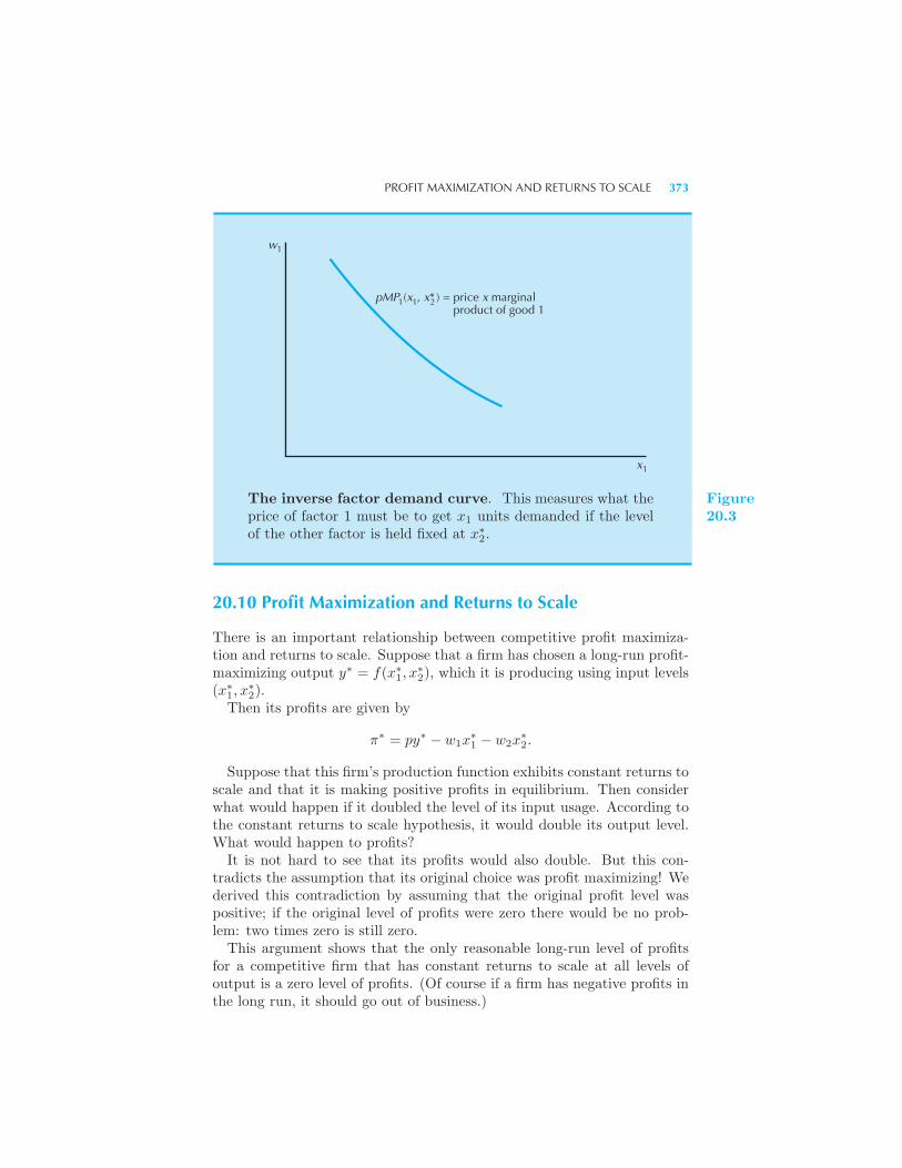
PROFIT MAXIMIZATION AND RETURNS TO SCALE 373
w
x
pMP (x , x* ) = price x marginal product of good 1
1 1 2
1
1
The inverse factor demand curve. This measures what theprice of factor 1 must be to get x1 units demanded if the levelof the other factor is held fixed at x∗
2.
Figure20.3
20.10 Profit Maximization and Returns to Scale
There is an important relationship between competitive profit maximiza-tion and returns to scale. Suppose that a firm has chosen a long-run profit-maximizing output y∗ = f(x∗
1, x∗2), which it is producing using input levels
(x∗1, x
∗2).
Then its profits are given by
π∗ = py∗ − w1x∗1 − w2x
∗2.
Suppose that this firm’s production function exhibits constant returns toscale and that it is making positive profits in equilibrium. Then considerwhat would happen if it doubled the level of its input usage. According tothe constant returns to scale hypothesis, it would double its output level.What would happen to profits?It is not hard to see that its profits would also double. But this con-
tradicts the assumption that its original choice was profit maximizing! Wederived this contradiction by assuming that the original profit level waspositive; if the original level of profits were zero there would be no prob-lem: two times zero is still zero.This argument shows that the only reasonable long-run level of profits
for a competitive firm that has constant returns to scale at all levels ofoutput is a zero level of profits. (Of course if a firm has negative profits inthe long run, it should go out of business.)
374 PROFIT MAXIMIZATION (Ch. 20)
Most people find this to be a surprising statement. Firms are out tomaximize profits aren’t they? How can it be that they can only get zeroprofits in the long run?Think about what would happen to a firm that did try to expand indef-
initely. Three things might occur. First, the firm could get so large that itcould not really operate effectively. This is just saying that the firm reallydoesn’t have constant returns to scale at all levels of output. Eventually,due to coordination problems, it might enter a region of decreasing returnsto scale.Second, the firm might get so large that it would totally dominate the
market for its product. In this case there is no reason for it to behavecompetitively—to take the price of output as given. Instead, it wouldmake sense for such a firm to try to use its size to influence the marketprice. The model of competitive profit maximization would no longer bea sensible way for the firm to behave, since it would effectively have nocompetitors. We’ll investigate more appropriate models of firm behaviorin this situation when we discuss monopoly.Third, if one firm can make positive profits with a constant returns to
scale technology, so can any other firm with access to the same technology.If one firm wants to expand its output, so would other firms. But if all firmsexpand their outputs, this will certainly push down the price of output andlower the profits of all the firms in the industry.
20.11 Revealed Profitability
When a profit-maximizing firm makes its choice of inputs and outputsit reveals two things: first, that the inputs and outputs used represent afeasible production plan, and second, that these choices are more profitablethan other feasible choices that the firm could have made. Let us examinethese points in more detail.Suppose that we observe two choices that the firm makes at two dif-
ferent sets of prices. At time t, it faces prices (pt, wt1, w
t2) and makes
choices (yt, xt1, x
t2). At time s, it faces prices (ps, ws
1, ws2) and makes choices
(ys, xs1, x
s2). If the production function of the firm hasn’t changed between
times s and t and if the firm is a profit maximizer, then we must have
ptyt − wt1x
t1 − wt
2xt2 ≥ ptys − wt
1xs1 − wt
2xs2 (20.2)
andpsys − ws
1xs1 − ws
2xs2 ≥ psyt − ws
1xt1 − ws
2xt2. (20.3)
That is, the profits that the firm achieved facing the t period prices must belarger than if they used the s period plan and vice versa. If either of theseinequalities were violated, the firm could not have been a profit-maximizingfirm (with an unchanging technology).
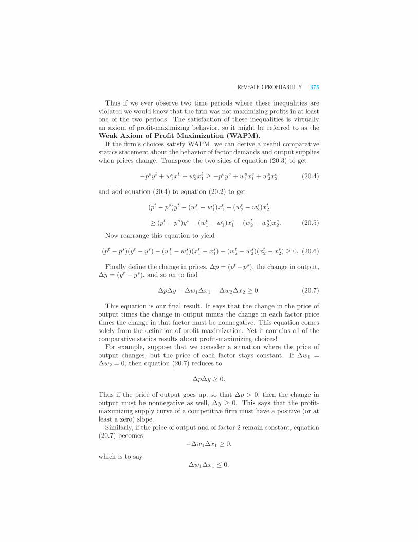
REVEALED PROFITABILITY 375
Thus if we ever observe two time periods where these inequalities areviolated we would know that the firm was not maximizing profits in at leastone of the two periods. The satisfaction of these inequalities is virtuallyan axiom of profit-maximizing behavior, so it might be referred to as theWeak Axiom of Profit Maximization (WAPM).If the firm’s choices satisfy WAPM, we can derive a useful comparative
statics statement about the behavior of factor demands and output supplieswhen prices change. Transpose the two sides of equation (20.3) to get
−psyt + ws1x
t1 + ws
2xt1 ≥ −psys + ws
1xs1 + ws
2xs2 (20.4)
and add equation (20.4) to equation (20.2) to get
(pt − ps)yt − (wt1 − ws
1)xt1 − (wt
2 − ws2)x
t2
≥ (pt − ps)ys − (wt1 − ws
1)xs1 − (wt
2 − ws2)x
s2. (20.5)
Now rearrange this equation to yield
(pt − ps)(yt − ys)− (wt1 − ws
1)(xt1 − xs
1)− (wt2 − ws
2)(xt2 − xs
2) ≥ 0. (20.6)
Finally define the change in prices, Δp = (pt−ps), the change in output,Δy = (yt − ys), and so on to find
ΔpΔy −Δw1Δx1 −Δw2Δx2 ≥ 0. (20.7)
This equation is our final result. It says that the change in the price ofoutput times the change in output minus the change in each factor pricetimes the change in that factor must be nonnegative. This equation comessolely from the definition of profit maximization. Yet it contains all of thecomparative statics results about profit-maximizing choices!For example, suppose that we consider a situation where the price of
output changes, but the price of each factor stays constant. If Δw1 =Δw2 = 0, then equation (20.7) reduces to
ΔpΔy ≥ 0.
Thus if the price of output goes up, so that Δp > 0, then the change inoutput must be nonnegative as well, Δy ≥ 0. This says that the profit-maximizing supply curve of a competitive firm must have a positive (or atleast a zero) slope.Similarly, if the price of output and of factor 2 remain constant, equation
(20.7) becomes−Δw1Δx1 ≥ 0,
which is to sayΔw1Δx1 ≤ 0.
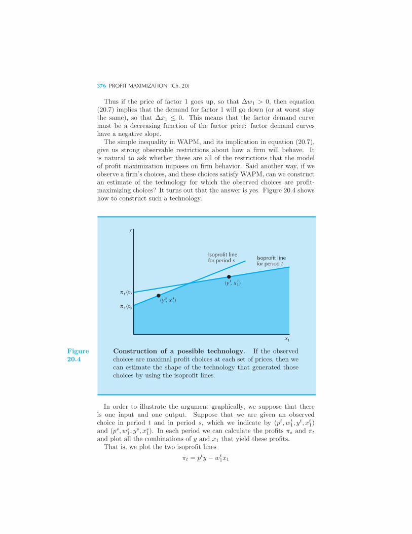
376 PROFIT MAXIMIZATION (Ch. 20)
Thus if the price of factor 1 goes up, so that Δw1 > 0, then equation(20.7) implies that the demand for factor 1 will go down (or at worst staythe same), so that Δx1 ≤ 0. This means that the factor demand curvemust be a decreasing function of the factor price: factor demand curveshave a negative slope.The simple inequality in WAPM, and its implication in equation (20.7),
give us strong observable restrictions about how a firm will behave. Itis natural to ask whether these are all of the restrictions that the modelof profit maximization imposes on firm behavior. Said another way, if weobserve a firm’s choices, and these choices satisfy WAPM, can we constructan estimate of the technology for which the observed choices are profit-maximizing choices? It turns out that the answer is yes. Figure 20.4 showshow to construct such a technology.
y
π /pt t
ssπ /p
Isoprofit linefor period s Isoprofit line
for period t
(y , x )s s1
x1
(y , x )t t1
Figure20.4
Construction of a possible technology. If the observedchoices are maximal profit choices at each set of prices, then wecan estimate the shape of the technology that generated thosechoices by using the isoprofit lines.
In order to illustrate the argument graphically, we suppose that thereis one input and one output. Suppose that we are given an observedchoice in period t and in period s, which we indicate by (pt, wt
1, yt, xt
1)and (ps, ws
1, ys, xs
1). In each period we can calculate the profits πs and πt
and plot all the combinations of y and x1 that yield these profits.That is, we plot the two isoprofit lines
πt = pty − wt1x1
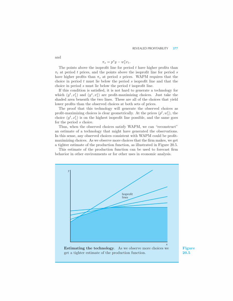
REVEALED PROFITABILITY 377
andπs = psy − ws
1x1.
The points above the isoprofit line for period t have higher profits thanπt at period t prices, and the points above the isoprofit line for period shave higher profits than πs at period s prices. WAPM requires that thechoice in period t must lie below the period s isoprofit line and that thechoice in period s must lie below the period t isoprofit line.If this condition is satisfied, it is not hard to generate a technology for
which (yt, xt1) and (ys, xs
1) are profit-maximizing choices. Just take theshaded area beneath the two lines. These are all of the choices that yieldlower profits than the observed choices at both sets of prices.The proof that this technology will generate the observed choices as
profit-maximizing choices is clear geometrically. At the prices (pt, wt1), the
choice (yt, xt1) is on the highest isoprofit line possible, and the same goes
for the period s choice.Thus, when the observed choices satisfy WAPM, we can “reconstruct”
an estimate of a technology that might have generated the observations.In this sense, any observed choices consistent with WAPM could be profit-maximizing choices. As we observe more choices that the firm makes, we geta tighter estimate of the production function, as illustrated in Figure 20.5.This estimate of the production function can be used to forecast firm
behavior in other environments or for other uses in economic analysis.
y
x
Isoprofitlines
Estimating the technology. As we observe more choices weget a tighter estimate of the production function.
Figure20.5
378 PROFIT MAXIMIZATION (Ch. 20)
EXAMPLE: How Do Farmers React to Price Supports?
The U.S. government currently spends between $40 and $60 billion a yearin aid to farmers. A large fraction of this amount is used to subsidizethe production of various products including milk, wheat, corn, soybeans,and cotton. Occasionally, attempts are made to reduce or eliminate thesesubsidies. The effect of elimination of these subsidies would be to reducethe price of the product received by the farmers.Farmers sometimes argue that eliminating the subsidies to milk, for ex-
ample, would not reduce the total supply of milk, since dairy farmers wouldchoose to increase their herds and their supply of milk so as to keep theirstandard of living constant.If farmers are behaving so as to maximize profits, this is impossible. As
we’ve seen above, the logic of profit maximization requires that a decreasein the price of an output leads to a reduction in its supply: if Δp is negative,then Δy must be negative as well.
It is certainly possible that small family farms have goals other than sim-ple maximization of profits, but larger “agribusiness” farms are more likelyto be profit maximizers. Thus the perverse response to the elimination ofsubsidies alluded to above could only occur on a limited scale, if at all.
20.12 Cost Minimization
If a firm is maximizing profits and if it chooses to supply some output y,then it must be minimizing the cost of producing y. If this were not so, thenthere would be some cheaper way of producing y units of output, whichwould mean that the firm was not maximizing profits in the first place.This simple observation turns out to be quite useful in examining firm
behavior. It turns out to be convenient to break the profit-maximizationproblem into two stages: first we figure out how to minimize the costs ofproducing any desired level of output y, then we figure out which level ofoutput is indeed a profit-maximizing level of output. We begin this task inthe next chapter.
Summary
1. Profits are the difference between revenues and costs. In this definitionit is important that all costs be measured using the appropriate marketprices.
2. Fixed factors are factors whose amount is independent of the level ofoutput; variable factors are factors whose amount used changes as the levelof output changes.
REVIEW QUESTIONS 379
3. In the short run, some factors must be used in predetermined amounts.In the long run, all factors are free to vary.
4. If the firm is maximizing profits, then the value of the marginal productof each factor that it is free to vary must equal its factor price.
5. The logic of profit maximization implies that the supply function of acompetitive firm must be an increasing function of the price of output andthat each factor demand function must be a decreasing function of its price.
6. If a competitive firm exhibits constant returns to scale, then its long-runmaximum profits must be zero.
REVIEW QUESTIONS
1. In the short run, if the price of the fixed factor is increased, what willhappen to profits?
2. If a firm had everywhere increasing returns to scale, what would happento its profits if prices remained fixed and if it doubled its scale of operation?
3. If a firm had decreasing returns to scale at all levels of output and itdivided up into two equal-size smaller firms, what would happen to itsoverall profits?
4. A gardener exclaims: “For only $1 in seeds I’ve grown over $20 in pro-duce!” Besides the fact that most of the produce is in the form of zucchini,what other observations would a cynical economist make about this situa-tion?
5. Is maximizing a firm’s profits always identical to maximizing the firm’sstock market value?
6. If pMP1 > w1, then should the firm increase or decrease the amount offactor 1 in order to increase profits?
7. Suppose a firm is maximizing profits in the short run with variable factorx1 and fixed factor x2. If the price of x2 goes down, what happens to thefirm’s use of x1? What happens to the firm’s level of profits?
8. A profit-maximizing competitive firm that is making positive profitsin long-run equilibrium (may/may not) have a technology with constantreturns to scale.
380 PROFIT MAXIMIZATION (Ch. 20)
APPENDIX
The profit-maximization problem of the firm is
maxx1,x2
pf(x1, x2)− w1x1 − w2x2,
which has first-order conditions
p∂f(x∗
1, x∗2)
∂x1− w1 = 0
p∂f(x∗
1, x∗2)
∂x2− w2 = 0.
These are just the same as the marginal product conditions given in the text.Let’s see how profit-maximizing behavior looks using the Cobb-Douglas produc-tion function.
Suppose the Cobb-Douglas function is given by f(x1, x2) = xa1x
b2. Then the
two first-order conditions become
paxa−11 xb
2 − w1 = 0
pbxa1x
b−12 − w2 = 0.
Multiply the first equation by x1 and the second equation by x2 to get
paxa1x
b2 − w1x1 = 0
pbxa1x
b2 − w2x2 = 0.
Using y = xa1x
b2 to denote the level of output of this firm we can rewrite these
expressions aspay = w1x1
pby = w2x2.
Solving for x1 and x2 we have
x∗1 =
apy
w1
x∗2 =
bpy
w2.
This gives us the demands for the two factors as a function of the optimal outputchoice. But we still have to solve for the optimal choice of output. Inserting theoptimal factor demands into the Cobb-Douglas production function, we have theexpression (
pay
w1
)a (pby
w2
)b
= y.
Factoring out the y gives
(pa
w1
)a ( pb
w2
)b
ya+b = y.
APPENDIX 381
Or
y =(pa
w1
) a1−a−b
(pb
w2
) b1−a−b
.
This gives us the supply function of the Cobb-Douglas firm. Along with thefactor demand functions derived above it gives us a complete solution to theprofit-maximization problem.
Note that when the firm exhibits constant returns to scale—when a+ b = 1—this supply function is not well defined. As long as the output and input prices areconsistent with zero profits, a firm with a Cobb-Douglas technology is indifferentabout its level of supply.
CHAPTER 21
COSTMINIMIZATION
Our goal is to study the behavior of profit-maximizing firms in both com-petitive and noncompetitive market environments. In the last chapter webegan our investigation of profit-maximizing behavior in a competitive en-vironment by examining the profit-maximization problem directly.
However, some important insights can be gained through a more indirectapproach. Our strategy will be to break up the profit-maximization prob-lem into two pieces. First, we will look at the problem of how to minimizethe costs of producing any given level of output, and then we will look athow to choose the most profitable level of output. In this chapter we’ll lookat the first step—minimizing the costs of producing a given level of output.
21.1 Cost Minimization
Suppose that we have two factors of production that have prices w1 andw2, and that we want to figure out the cheapest way to produce a givenlevel of output, y. If we let x1 and x2 measure the amounts used of the
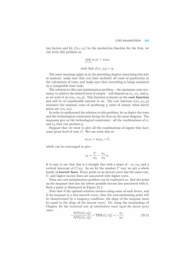
COST MINIMIZATION 383
two factors and let f(x1, x2) be the production function for the firm, wecan write this problem as
minx1,x2
w1x1 + w2x2
such that f(x1, x2) = y.
The same warnings apply as in the preceding chapter concerning this sortof analysis: make sure that you have included all costs of production inthe calculation of costs, and make sure that everything is being measuredon a compatible time scale.The solution to this cost-minimization problem—the minimum costs nec-
essary to achieve the desired level of output—will depend on w1, w2, and y,so we write it as c(w1, w2, y). This function is known as the cost functionand will be of considerable interest to us. The cost function c(w1, w2, y)measures the minimal costs of producing y units of output when factorprices are (w1, w2).In order to understand the solution to this problem, let us depict the costs
and the technological constraints facing the firm on the same diagram. Theisoquants give us the technological constraints—all the combinations of x1
and x2 that can produce y.Suppose that we want to plot all the combinations of inputs that have
some given level of cost, C. We can write this as
w1x1 + w2x2 = C,
which can be rearranged to give
x2 =C
w2− w1
w2x1.
It is easy to see that this is a straight line with a slope of −w1/w2 and avertical intercept of C/w2. As we let the number C vary we get a wholefamily of isocost lines. Every point on an isocost curve has the same cost,C, and higher isocost lines are associated with higher costs.Thus our cost-minimization problem can be rephrased as: find the point
on the isoquant that has the lowest possible isocost line associated with it.Such a point is illustrated in Figure 21.1.Note that if the optimal solution involves using some of each factor, and
if the isoquant is a nice smooth curve, then the cost-minimizing point willbe characterized by a tangency condition: the slope of the isoquant mustbe equal to the slope of the isocost curve. Or, using the terminology ofChapter 19, the technical rate of substitution must equal the factor priceratio:
−MP1(x∗1, x
∗2)
MP2(x∗1, x
∗2)
= TRS(x∗1, x
∗2) = −w1
w2. (21.1)
384 COST MINIMIZATION (Ch. 21)
Optimal choice
x
x*
x*
Isoquantf (x , x ) = y1 2
Isocost linesslope = –w /w21
2
2
1 x1
Figure21.1
Cost minimization. The choice of factors that minimize pro-duction costs can be determined by finding the point on theisoquant that has the lowest associated isocost curve.
(If we have a boundary solution where one of the two factors isn’t used,this tangency condition need not be met. Similarly, if the production func-tion has “kinks,” the tangency condition has no meaning. These exceptionsare just like the situation with the consumer, so we won’t emphasize thesecases in this chapter.)
The algebra that lies behind equation (21.1) is not difficult. Considerany change in the pattern of production (Δx1,Δx2) that keeps outputconstant. Such a change must satisfy
MP1(x∗1, x
∗2)Δx1 +MP2(x
∗1, x
∗2)Δx2 = 0. (21.2)
Note that Δx1 and Δx2 must be of opposite signs; if you increase theamount used of factor 1 you must decrease the amount used of factor 2 inorder to keep output constant.
If we are at the cost minimum, then this change cannot lower costs, sowe have
w1Δx1 + w2Δx2 ≥ 0. (21.3)
Now consider the change (−Δx1,−Δx2). This also produces a constantlevel of output, and it too cannot lower costs. This implies that
−w1Δx1 − w2Δx2 ≥ 0. (21.4)
COST MINIMIZATION 385
Putting expressions (21.3) and (21.4) together gives us
w1Δx1 + w2Δx2 = 0. (21.5)
Solving equations (21.2) and (21.5) for Δx2/Δx1 gives
Δx2
Δx1= −w1
w2= −MP1(x
∗1, x
∗2)
MP2(x∗1, x
∗2),
which is just the condition for cost minimization derived above by a geo-metric argument.Note that Figure 21.1 bears a certain resemblance to the solution to
the consumer-choice problem depicted earlier. Although the solutions lookthe same, they really aren’t the same kind of problem. In the consumerproblem, the straight line was the budget constraint, and the consumermoved along the budget constraint to find the most-preferred position. Inthe producer problem, the isoquant is the technological constraint and theproducer moves along the isoquant to find the optimal position.The choices of inputs that yield minimal costs for the firm will in general
depend on the input prices and the level of output that the firm wantsto produce, so we write these choices as x1(w1, w2, y) and x2(w1, w2, y).These are called the conditional factor demand functions, or derivedfactor demands. They measure the relationship between the prices andoutput and the optimal factor choice of the firm, conditional on the firmproducing a given level of output, y.Note carefully the difference between the conditional factor demands and
the profit-maximizing factor demands discussed in the last chapter. Theconditional factor demands give the cost-minimizing choices for a given levelof output; the profit-maximizing factor demands give the profit-maximizingchoices for a given price of output.Conditional factor demands are usually not directly observed; they are
a hypothetical construct. They answer the question of how much of eachfactor would the firm use if it wanted to produce a given level of outputin the cheapest way. However, the conditional factor demands are usefulas a way of separating the problem of determining the optimal level ofoutput from the problem of determining the most cost-effective method ofproduction.
EXAMPLE: Minimizing Costs for Specific Technologies
Suppose that we consider a technology where the factors are perfect com-plements, so that f(x1, x2) = min{x1, x2}. Then if we want to produce yunits of output, we clearly need y units of x1 and y units of x2. Thus theminimal costs of production will be
c(w1, w2, y) = w1y + w2y = (w1 + w2)y.
386 COST MINIMIZATION (Ch. 21)
What about the perfect substitutes technology, f(x1, x2) = x1 + x2?Since goods 1 and 2 are perfect substitutes in production it is clear thatthe firm will use whichever is cheaper. Thus the minimum cost of producingy units of output will be w1y or w2y, whichever is less. In other words:
c(w1, w2, y) = min{w1y, w2y} = min{w1, w2}y.
Finally, we consider the Cobb-Douglas technology, which is described bythe formula f(x1, x2) = xa
1xb2. In this case we can use calculus techniques
to show that the cost function will have the form
c(w1, w2, y) = Kwa
a+b
1 wb
a+b
2 y1
a+b ,
where K is a constant that depends on a and b. The details of the calcu-lation are presented in the Appendix.
21.2 Revealed Cost Minimization
The assumption that the firm chooses factors to minimize the cost of pro-ducing output will have implications for how the observed choices changeas factor prices change.Suppose that we observe two sets of prices, (wt
1, wt2) and (ws
1, ws2), and
the associated choices of the firm, (xt1, x
t2) and (xs
1, xs2). Suppose that each
of these choices produces the same output level y. Then if each choice is acost-minimizing choice at its associated prices, we must have
wt1x
t1 + wt
2xt2 ≤ wt
1xs1 + wt
2xs2
andws
1xs1 + ws
2xs2 ≤ ws
1xt1 + ws
2xt2.
If the firm is always choosing the cost-minimizing way to produce y unitsof output, then its choices at times t and s must satisfy these inequali-ties. We will refer to these inequalities as the Weak Axiom of CostMinimization (WACM).Write the second equation as
−ws1x
t1 − ws
2xt2 ≤ −ws
1xs1 − ws
2xs2
and add it to the first equation to get
(wt1 − ws
1)xt1 + (wt
2 − ws2)x
t2 ≤ (wt
1 − ws1)x
s1 + (wt
2 − ws2)x
s2,
which can be rearranged to give us
(wt1 − ws
1)(xt1 − xs
1) + (wt2 − ws
2)(xt2 − xs
2) ≤ 0.
RETURNS TO SCALE AND THE COST FUNCTION 387
Using the delta notation to depict the changes in the factor demandsand factor prices, we have
Δw1Δx1 +Δw2Δx2 ≤ 0.
This equation follows solely from the assumption of cost-minimizing be-havior. It implies restrictions on how the firm’s behavior can change wheninput prices change and output remains constant.For example, if the price of the first factor increases and the price of the
second factor stays constant, then Δw2 = 0, so the inequality becomes
Δw1Δx1 ≤ 0.
If the price of factor 1 increases, then this inequality implies that thedemand for factor 1 must decrease; thus the conditional factor demandfunctions must slope down.What can we say about how the minimal costs change as we change the
parameters of the problem? It is easy to see that costs must increase ifeither factor price increases: if one good becomes more expensive and theother stays the same, the minimal costs cannot go down and in general willincrease. Similarly, if the firm chooses to produce more output and factorprices remain constant, the firm’s costs will have to increase.
21.3 Returns to Scale and the Cost Function
In Chapter 19 we discussed the idea of returns to scale for the productionfunction. Recall that a technology is said to have increasing, decreasing,or constant returns to scale as f(tx1, tx2) is greater, less than, or equal totf(x1, x2) for all t > 1. It turns out that there is a nice relation betweenthe kind of returns to scale exhibited by the production function and thebehavior of the cost function.Suppose first that we have the natural case of constant returns to scale.
Imagine that we have solved the cost-minimization problem to produce 1unit of output, so that we know the unit cost function, c(w1, w2, 1). Nowwhat is the cheapest way to produce y units of output? Simple: we justuse y times as much of every input as we were using to produce 1 unitof output. This would mean that the minimal cost to produce y units ofoutput would just be c(w1, w2, 1)y. In the case of constant returns to scale,the cost function is linear in output.What if we have increasing returns to scale? In this case it turns out that
costs increase less than linearly in output. If the firm decides to producetwice as much output, it can do so at less than twice the cost, as long asthe factor prices remain fixed. This is a natural implication of the idea ofincreasing returns to scale: if the firm doubles its inputs, it will more than
388 COST MINIMIZATION (Ch. 21)
double its output. Thus if it wants to produce double the output, it willbe able to do so by using less than twice as much of every input.But using twice as much of every input will exactly double costs. So
using less than twice as much of every input will make costs go up by lessthan twice as much: this is just saying that the cost function will increaseless than linearly with respect to output.Similarly, if the technology exhibits decreasing returns to scale, the cost
function will increase more than linearly with respect to output. If outputdoubles, costs will more than double.These facts can be expressed in terms of the behavior of the average
cost function. The average cost function is simply the cost per unit toproduce y units of output:
AC(y) =c(w1, w2, y)
y.
If the technology exhibits constant returns to scale, then we saw abovethat the cost function had the form c(w1, w2, y) = c(w1, w2, 1)y. Thismeans that the average cost function will be
AC(w1, w2, y) =c(w1, w2, 1)y
y= c(w1, w2, 1).
That is, the cost per unit of output will be constant no matter what levelof output the firm wants to produce.If the technology exhibits increasing returns to scale, then the costs will
increase less than linearly with respect to output, so the average costs willbe declining in output: as output increases, the average costs of productionwill tend to fall.Similarly, if the technology exhibits decreasing returns to scale, then
average costs will rise as output increases.As we saw earlier, a given technology can have regions of increasing,
constant, or decreasing returns to scale—output can increase more rapidly,equally rapidly, or less rapidly than the scale of operation of the firm atdifferent levels of production. Similarly, the cost function can increase lessrapidly, equally rapidly, or more rapidly than output at different levelsof production. This implies that the average cost function may decrease,remain constant, or increase over different levels of output. In the nextchapter we will explore these possibilities in more detail.From now on we will be most concerned with the behavior of the cost
function with respect to the output variable. For the most part we willregard the factor prices as being fixed at some predetermined levels andonly think of costs as depending on the output choice of the firm. Thus forthe remainder of the book we will write the cost function as a function ofoutput alone: c(y).
LONG-RUN AND SHORT-RUN COSTS 389
21.4 Long-Run and Short-Run Costs
The cost function is defined as the minimum cost of achieving a given levelof output. Often it is important to distinguish the minimum costs if thefirm is allowed to adjust all of its factors of production from the minimumcosts if the firm is only allowed to adjust some of its factors.We have defined the short run to be a time period where some of the
factors of production must be used in a fixed amount. In the long run,all factors are free to vary. The short-run cost function is defined asthe minimum cost to produce a given level of output, only adjusting thevariable factors of production. The long-run cost function gives theminimum cost of producing a given level of output, adjusting all of thefactors of production.Suppose that in the short run factor 2 is fixed at some predetermined
level x2, but in the long run it is free to vary. Then the short-run costfunction is defined by
cs(y, x2) = minx1
w1x1 + w2x2
such that f(x1, x2) = y.
Note that in general the minimum cost to produce y units of output in theshort run will depend on the amount and cost of the fixed factor that isavailable.In the case of two factors, this minimization problem is easy to solve: we
just find the smallest amount of x1 such that f(x1, x2) = y. However, ifthere are many factors of production that are variable in the short run thecost-minimization problem will involve more elaborate calculation.The short-run factor demand function for factor 1 is the amount of fac-
tor 1 that minimizes costs. In general it will depend on the factor pricesand on the levels of the fixed factors as well, so we write the short-runfactor demands as
x1 = xs1(w1, w2, x2, y)
x2 = x2.
These equations just say, for example, that if the building size is fixedin the short run, then the number of workers that a firm wants to hire atany given set of prices and output choice will typically depend on the sizeof the building.Note that by definition of the short-run cost function
cs(y, x2) = w1xs1(w1, w2, x2, y) + w2x2.
This just says that the minimum cost of producing output y is the costassociated with using the cost-minimizing choice of inputs. This is true bydefinition but turns out to be useful nevertheless.
390 COST MINIMIZATION (Ch. 21)
The long-run cost function in this example is defined by
c(y) = minx1,x2
w1x1 + w2x2
such that f(x1, x2) = y.
Here both factors are free to vary. Long-run costs depend only on the levelof output that the firm wants to produce along with factor prices. We writethe long-run cost function as c(y), and write the long-run factor demandsas
x1 = x1(w1, w2, y)
x2 = x2(w1, w2, y).
We can also write the long-run cost function as
c(y) = w1x1(w1, w2, y) + w2x2(w1, w2, y).
Just as before, this simply says that the minimum costs are the costs thatthe firm gets by using the cost-minimizing choice of factors.
There is an interesting relation between the short-run and the long-runcost functions that we will use in the next chapter. For simplicity, let ussuppose that factor prices are fixed at some predetermined levels and writethe long-run factor demands as
x1 = x1(y)
x2 = x2(y).
Then the long-run cost function can also be written as
c(y) = cs(y, x2(y)).
To see why this is true, just think about what it means. The equation saysthat the minimum costs when all factors are variable is just the minimumcost when factor 2 is fixed at the level that minimizes long-run costs. It fol-lows that the long-run demand for the variable factor—the cost-minimizingchoice—is given by
x1(w1, w2, y) = xs1(w1, w2, x2(y), y).
This equation says that the cost-minimizing amount of the variable factorin the long run is that amount that the firm would choose in the shortrun—if it happened to have the long-run cost-minimizing amount of thefixed factor.
SUNK COSTS 391
21.5 Fixed and Quasi-Fixed Costs
In Chapter 20 we made the distinction between fixed factors and quasi-fixed factors. Fixed factors are factors that must receive payment whetheror not any output is produced. Quasi-fixed factors must be paid only if thefirm decides to produce a positive amount of output.
It is natural to define fixed costs and quasi-fixed costs in a similar man-ner. Fixed costs are costs associated with the fixed factors: they areindependent of the level of output, and, in particular, they must be paidwhether or not the firm produces output. Quasi-fixed costs are coststhat are also independent of the level of output, but only need to be paidif the firm produces a positive amount of output.
There are no fixed costs in the long run, by definition. However, theremay easily be quasi-fixed costs in the long run. If it is necessary to spenda fixed amount of money before any output at all can be produced, thenquasi-fixed costs will be present.
21.6 Sunk Costs
Sunk costs are another kind of fixed costs. The concept is best explained byexample. Suppose that you have decided to lease an office for a year. Themonthly rent that you have committed to pay is a fixed cost, since you areobligated to pay it regardless of the amount of output you produce. Nowsuppose that you decide to refurbish the office by painting it and buyingfurniture. The cost for paint is a fixed cost, but it is also a sunk cost sinceit is a payment that is made and cannot be recovered. The cost of buyingthe furniture, on the other hand, is not entirely sunk, since you can resellthe furniture when you are done with it. It’s only the difference betweenthe cost of new and used furniture that is sunk.
To spell this out in more detail, suppose that you borrow $20,000 at thebeginning of the year at, say, 10 percent interest. You sign a lease to rentan office and pay $12,000 in advance rent for next year. You spend $6,000on office furniture and $2,000 to paint the office. At the end of the yearyou pay back the $20,000 loan plus the $2,000 interest payment and sellthe used office furniture for $5,000.
Your total sunk costs consist of the $12,000 rent, the $2,000 of interest,the $2,000 of paint, but only $1,000 for the furniture, since $5,000 of theorginal furniture expenditure is recoverable.
The difference between sunk costs and recoverable costs can be quitesignificant. A $100,000 expenditure to purchase five light trucks soundslike a lot of money, but if they can later be sold on the used truck marketfor $80,000, the actual sunk cost is only $20,000. A $100,000 expenditure
392 COST MINIMIZATION (Ch. 21)
on a custom-made press for stamping out gizmos that has a zero resalevalue is quite different; in this case the entire expenditure is sunk.The best way to keep these issues straight is to make sure to treat all
expenditures on a flow basis: how much does it cost to do business fora year? That way, one is less likely to forget the resale value of capitalequipment and more likely to keep the distinction between sunk costs andrecoverable costs clear.
Summary
1. The cost function, c(w1, w2, y), measures the minimum costs of produc-ing a given level of output at given factor prices.
2. Cost-minimizing behavior imposes observable restrictions on choices thatfirms make. In particular, conditional factor demand functions will be neg-atively sloped.
3. There is an intimate relationship between the returns to scale exhibitedby the technology and the behavior of the cost function. Increasing returnsto scale implies decreasing average cost, decreasing returns to scale impliesincreasing average cost, and constant returns to scale implies constant av-erage cost.
4. Sunk costs are costs that are not recoverable.
REVIEW QUESTIONS
1. Prove that a profit-maximizing firm will always minimize costs.
2. If a firm is producing where MP1/w1 > MP2/w2, what can it do toreduce costs but maintain the same output?
3. Suppose that a cost-minimizing firm uses two inputs that are perfectsubstitutes. If the two inputs are priced the same, what do the conditionalfactor demands look like for the inputs?
4. The price of paper used by a cost-minimizing firm increases. The firmresponds to this price change by changing its demand for certain inputs,but it keeps its output constant. What happens to the firm’s use of paper?
5. If a firm uses n inputs (n > 2), what inequality does the theory ofrevealed cost minimization imply about changes in factor prices (Δwi) andthe changes in factor demands (Δxi) for a given level of output?
APPENDIX 393
APPENDIX
Let us study the cost-minimization problem posed in the text using the opti-mization techniques introduced in Chapter 5. The problem is a constrained-minimization problem of the form
minx1,x2
w1x1 + w2x2
such that f(x1, x2) = y.
Recall that we had several techniques to solve this kind of problem. One waywas to substitute the constraint into the objective function. This can still beused when we have a specific functional form for f(x1, x2), but isn’t much use inthe general case.
The second method was the method of Lagrange multipliers and that worksfine. To apply this method we set up the Lagrangian
L = w1x1 + w2x2 − λ(f(x1, x2)− y)
and differentiate with respect to x1, x2 and λ. This gives us the first-orderconditions:
w1 − λ∂f(x1, x2)
∂x1= 0
w2 − λ∂f(x1, x2)
∂x2= 0
f(x1, x2)− y = 0.
The last condition is simply the constraint. We can rearrange the first twoequations and divide the first equation by the second equation to get
w1
w2=
∂f(x1, x2)/∂x1
∂f(x1, x2)/∂x2.
Note that this is the same first-order condition that we derived in the text: thetechnical rate of substitution must equal the factor price ratio.
Let’s apply this method to the Cobb-Douglas production function:
f(x1, x2) = xa1x
b2.
The cost-minimization problem is then
minx1,x2
w1x1 + w2x2
such that xa1x
b2 = y.
Here we have a specific functional form, and we can solve it using either thesubstitution method or the Lagrangian method. The substitution method wouldinvolve first solving the constraint for x2 as a function of x1:
x2 =(yx−a
1
)1/b
394 COST MINIMIZATION (Ch. 21)
and then substituting this into the objective function to get the unconstrainedminimization problem
minx1
w1x1 + w2
(yx−a
1
)1/b.
We could now differentiate with respect to x1 and set resulting derivative equalto zero, as usual. The resulting equation can be solved to get x1 as a functionof w1, w2, and y, to get the conditional factor demand for x1. This isn’t hard todo, but the algebra is messy, so we won’t write down the details.
We will, however, solve the Lagrangian problem. The three first-order condi-tions are
w1 = λaxa−11 xb
2
w2 = λbxa1x
b−12
y = xa1x
b2.
Multiply the first equation by x1 and the second equation by x2 to get
w1x1 = λaxa1x
b2 = λay
w2x2 = λbxa1x
b2 = λby,
so that
x1 = λay
w1(21.6)
x2 = λby
w2. (21.7)
Now we use the third equation to solve for λ. Substituting the solutions for x1
and x2 into the third first-order condition, we have
(λay
w1
)a (λby
w2
)b
= y.
We can solve this equation for λ to get the rather formidable expression
λ = (a−ab−bwa1w
b2y
1−a−b)1
a+b ,
which, along with equations (21.6) and (21.7), gives us our final solutions for x1
and x2. These factor demand functions will take the form
x1(w1, w2, y) =(a
b
) ba+b
w−ba+b
1 wb
a+b
2 y1
a+b
x2(w1, w2, y) =(a
b
)− aa+b
wa
a+b
1 w−aa+b
2 y1
a+b .
The cost function can be found by writing down the costs when the firm makesthe cost-minimizing choices. That is,
c(w1, w2, y) = w1x1(w1, w2, y) + w2x2(w1, w2, y).
APPENDIX 395
Some tedious algebra shows that
c(w1, w2, y) =
[(a
b
) ba+b
+(a
b
) −aa+b
]w
aa+b
1 wb
a+b
2 y1
a+b .
(Don’t worry, this formula won’t be on the final exam. It is presented only todemonstrate how to get an explicit solution to the cost-minimization problem byapplying the method of Lagrange multipliers.)
Note that costs will increase more than, equal to, or less than linearly withoutput as a+ b is less than, equal to, or greater than 1. This makes sense sincethe Cobb-Douglas technology exhibits decreasing, constant, or increasing returnsto scale depending on the value of a+ b.
CHAPTER 22
COSTCURVES
In the last chapter we described the cost-minimizing behavior of a firm.Here we continue that investigation through the use of an important geo-metric construction, the cost curve. Cost curves can be used to depictgraphically the cost function of a firm and are important in studying thedetermination of optimal output choices.
22.1 Average Costs
Consider the cost function described in the last chapter. This is the functionc(w1, w2, y) that gives the minimum cost of producing output level y whenfactor prices are (w1, w2). In the rest of this chapter we will take the factorprices to be fixed so that we can write cost as a function of y alone, c(y).
Some of the costs of the firm are independent of the level of output ofthe firm. As we’ve seen in Chapter 21, these are the fixed costs. Fixedcosts are the costs that must be paid regardless of what level of output thefirm produces. For example, the firm might have mortgage payments thatare required no matter what its level of output.
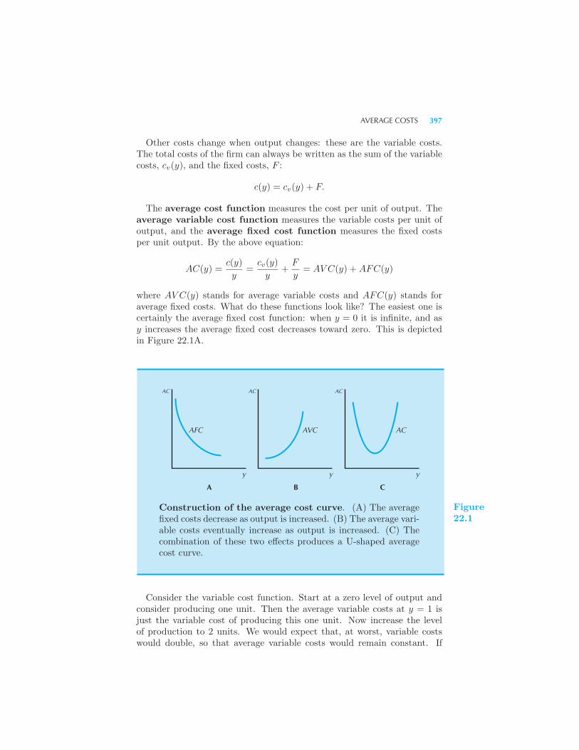
AVERAGE COSTS 397
Other costs change when output changes: these are the variable costs.The total costs of the firm can always be written as the sum of the variablecosts, cv(y), and the fixed costs, F :
c(y) = cv(y) + F.
The average cost function measures the cost per unit of output. Theaverage variable cost function measures the variable costs per unit ofoutput, and the average fixed cost function measures the fixed costsper unit output. By the above equation:
AC(y) =c(y)
y=
cv(y)
y+
F
y= AV C(y) +AFC(y)
where AV C(y) stands for average variable costs and AFC(y) stands foraverage fixed costs. What do these functions look like? The easiest one iscertainly the average fixed cost function: when y = 0 it is infinite, and asy increases the average fixed cost decreases toward zero. This is depictedin Figure 22.1A.
AC AC AC
AVC ACAFC
y y y
A B C
Construction of the average cost curve. (A) The averagefixed costs decrease as output is increased. (B) The average vari-able costs eventually increase as output is increased. (C) Thecombination of these two effects produces a U-shaped averagecost curve.
Figure22.1
Consider the variable cost function. Start at a zero level of output andconsider producing one unit. Then the average variable costs at y = 1 isjust the variable cost of producing this one unit. Now increase the levelof production to 2 units. We would expect that, at worst, variable costswould double, so that average variable costs would remain constant. If
398 COST CURVES (Ch. 22)
we can organize production in a more efficient way as the scale of outputis increased, the average variable costs might even decrease initially. Buteventually we would expect the average variable costs to rise. Why? If fixedfactors are present, they will eventually constrain the production process.For example, suppose that the fixed costs are due to the rent or mortgage
payments on a building of fixed size. Then as production increases, averagevariable costs—the per-unit production costs—may remain constant for awhile. But as the capacity of the building is reached, these costs will risesharply, producing an average variable cost curve of the form depicted inFigure 22.1B.The average cost curve is the sum of these two curves; thus it will have
the U-shape indicated in Figure 22.1C. The initial decline in average costsis due to the decline in average fixed costs; the eventual increase in averagecosts is due to the increase in average variable costs. The combination ofthese two effects yields the U-shape depicted in the diagram.
22.2 Marginal Costs
There is one more cost curve of interest: the marginal cost curve. Themarginal cost curve measures the change in costs for a given change inoutput. That is, at any given level of output y, we can ask how costs willchange if we change output by some amount Δy:
MC(y) =Δc(y)
Δy=
c(y +Δy)− c(y)
Δy.
We could just as well write the definition of marginal costs in terms ofthe variable cost function:
MC(y) =Δcv(y)
Δy=
cv(y +Δy)− cv(y)
Δy.
This is equivalent to the first definition, since c(y) = cv(y) + F and thefixed costs, F , don’t change as y changes.Often we think of Δy as being one unit of output, so that marginal
cost indicates the change in our costs if we consider producing one morediscrete unit of output. If we are thinking of the production of a discretegood, then marginal cost of producing y units of output is just c(y) −c(y − 1). This is often a convenient way to think about marginal cost,but is sometimes misleading. Remember, marginal cost measures a rate ofchange: the change in costs divided by a change in output. If the changein output is a single unit, then marginal cost looks like a simple changein costs, but it is really a rate of change as we increase the output by oneunit.
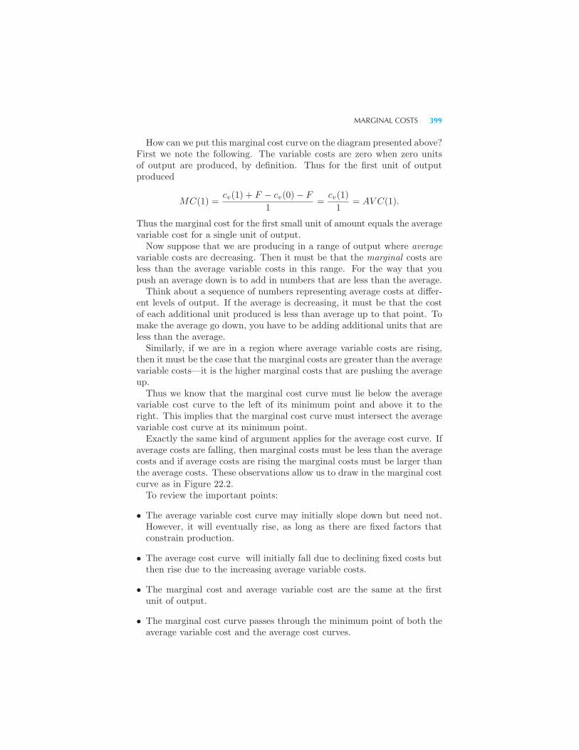
MARGINAL COSTS 399
How can we put this marginal cost curve on the diagram presented above?First we note the following. The variable costs are zero when zero unitsof output are produced, by definition. Thus for the first unit of outputproduced
MC(1) =cv(1) + F − cv(0)− F
1=
cv(1)
1= AV C(1).
Thus the marginal cost for the first small unit of amount equals the averagevariable cost for a single unit of output.Now suppose that we are producing in a range of output where average
variable costs are decreasing. Then it must be that the marginal costs areless than the average variable costs in this range. For the way that youpush an average down is to add in numbers that are less than the average.Think about a sequence of numbers representing average costs at differ-
ent levels of output. If the average is decreasing, it must be that the costof each additional unit produced is less than average up to that point. Tomake the average go down, you have to be adding additional units that areless than the average.Similarly, if we are in a region where average variable costs are rising,
then it must be the case that the marginal costs are greater than the averagevariable costs—it is the higher marginal costs that are pushing the averageup.Thus we know that the marginal cost curve must lie below the average
variable cost curve to the left of its minimum point and above it to theright. This implies that the marginal cost curve must intersect the averagevariable cost curve at its minimum point.Exactly the same kind of argument applies for the average cost curve. If
average costs are falling, then marginal costs must be less than the averagecosts and if average costs are rising the marginal costs must be larger thanthe average costs. These observations allow us to draw in the marginal costcurve as in Figure 22.2.To review the important points:
• The average variable cost curve may initially slope down but need not.However, it will eventually rise, as long as there are fixed factors thatconstrain production.
• The average cost curve will initially fall due to declining fixed costs butthen rise due to the increasing average variable costs.
• The marginal cost and average variable cost are the same at the firstunit of output.
• The marginal cost curve passes through the minimum point of both theaverage variable cost and the average cost curves.
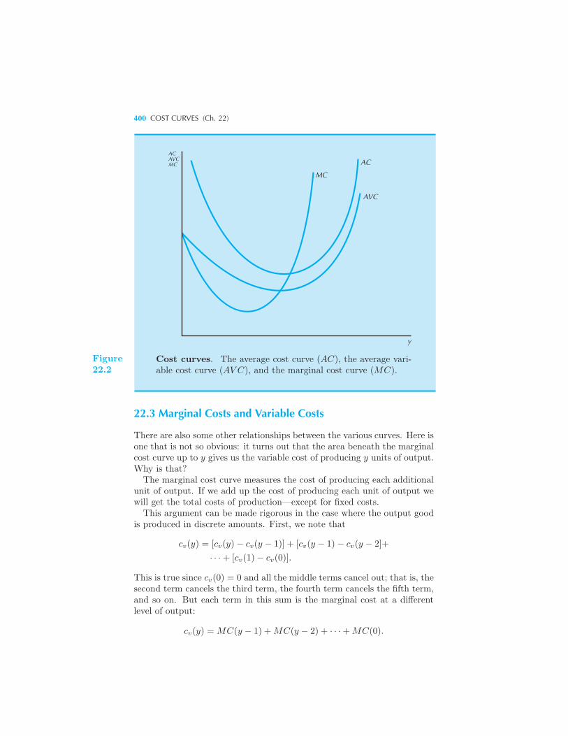
400 COST CURVES (Ch. 22)
ACAVCMC
MC
AC
AVC
y
Figure22.2
Cost curves. The average cost curve (AC), the average vari-able cost curve (AV C), and the marginal cost curve (MC).
22.3 Marginal Costs and Variable Costs
There are also some other relationships between the various curves. Here isone that is not so obvious: it turns out that the area beneath the marginalcost curve up to y gives us the variable cost of producing y units of output.Why is that?The marginal cost curve measures the cost of producing each additional
unit of output. If we add up the cost of producing each unit of output wewill get the total costs of production—except for fixed costs.This argument can be made rigorous in the case where the output good
is produced in discrete amounts. First, we note that
cv(y) = [cv(y)− cv(y − 1)] + [cv(y − 1)− cv(y − 2]+
· · ·+ [cv(1)− cv(0)].
This is true since cv(0) = 0 and all the middle terms cancel out; that is, thesecond term cancels the third term, the fourth term cancels the fifth term,and so on. But each term in this sum is the marginal cost at a differentlevel of output:
cv(y) = MC(y − 1) +MC(y − 2) + · · ·+MC(0).
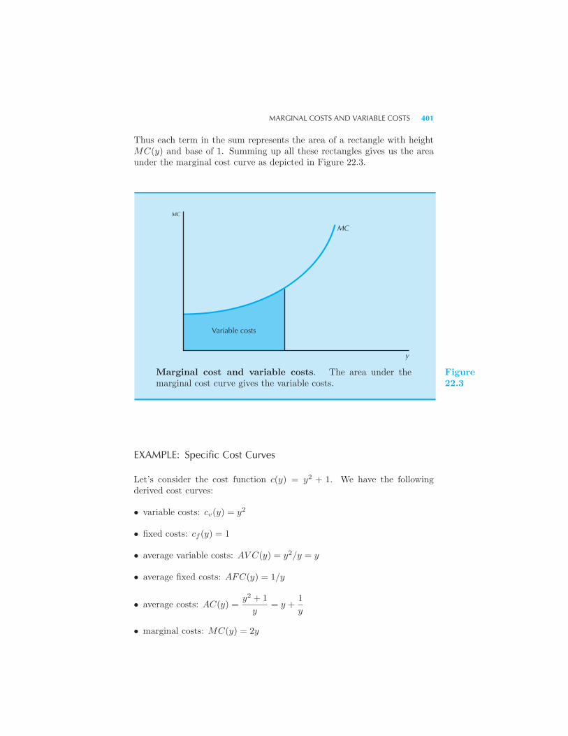
MARGINAL COSTS AND VARIABLE COSTS 401
Thus each term in the sum represents the area of a rectangle with heightMC(y) and base of 1. Summing up all these rectangles gives us the areaunder the marginal cost curve as depicted in Figure 22.3.
MC
MC
Variable costs
y
Marginal cost and variable costs. The area under themarginal cost curve gives the variable costs.
Figure22.3
EXAMPLE: Specific Cost Curves
Let’s consider the cost function c(y) = y2 + 1. We have the followingderived cost curves:
• variable costs: cv(y) = y2
• fixed costs: cf (y) = 1
• average variable costs: AV C(y) = y2/y = y
• average fixed costs: AFC(y) = 1/y
• average costs: AC(y) =y2 + 1
y= y +
1
y
• marginal costs: MC(y) = 2y
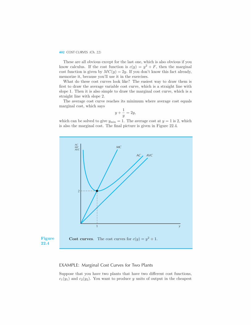
402 COST CURVES (Ch. 22)
These are all obvious except for the last one, which is also obvious if youknow calculus. If the cost function is c(y) = y2 + F , then the marginalcost function is given by MC(y) = 2y. If you don’t know this fact already,memorize it, because you’ll use it in the exercises.What do these cost curves look like? The easiest way to draw them is
first to draw the average variable cost curve, which is a straight line withslope 1. Then it is also simple to draw the marginal cost curve, which is astraight line with slope 2.The average cost curve reaches its minimum where average cost equals
marginal cost, which says
y +1
y= 2y,
which can be solved to give ymin = 1. The average cost at y = 1 is 2, whichis also the marginal cost. The final picture is given in Figure 22.4.
2
1
ACMCAVC
MC
AC AVC
y
Figure22.4
Cost curves. The cost curves for c(y) = y2 + 1.
EXAMPLE: Marginal Cost Curves for Two Plants
Suppose that you have two plants that have two different cost functions,c1(y1) and c2(y2). You want to produce y units of output in the cheapest
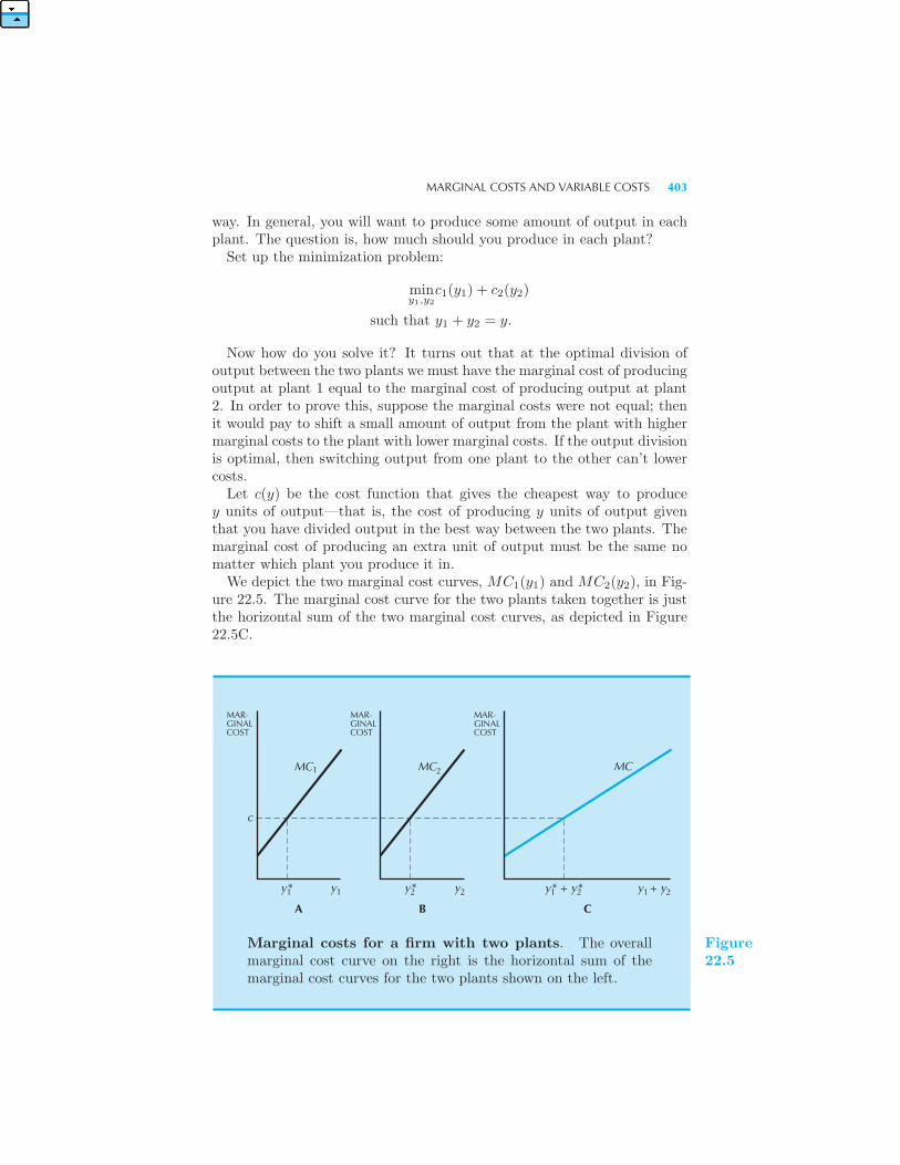
MARGINAL COSTS AND VARIABLE COSTS 403
way. In general, you will want to produce some amount of output in eachplant. The question is, how much should you produce in each plant?Set up the minimization problem:
miny1,y2
c1(y1) + c2(y2)
such that y1 + y2 = y.
Now how do you solve it? It turns out that at the optimal division ofoutput between the two plants we must have the marginal cost of producingoutput at plant 1 equal to the marginal cost of producing output at plant2. In order to prove this, suppose the marginal costs were not equal; thenit would pay to shift a small amount of output from the plant with highermarginal costs to the plant with lower marginal costs. If the output divisionis optimal, then switching output from one plant to the other can’t lowercosts.Let c(y) be the cost function that gives the cheapest way to produce
y units of output—that is, the cost of producing y units of output giventhat you have divided output in the best way between the two plants. Themarginal cost of producing an extra unit of output must be the same nomatter which plant you produce it in.We depict the two marginal cost curves, MC1(y1) and MC2(y2), in Fig-
ure 22.5. The marginal cost curve for the two plants taken together is justthe horizontal sum of the two marginal cost curves, as depicted in Figure22.5C.
MAR-GINALCOST
MC MC MC
c
y* y yy*
A B C
y* + y* y + y1 2 1 2
21
21 1 2
MAR-GINALCOST
MAR-GINALCOST
Marginal costs for a firm with two plants. The overallmarginal cost curve on the right is the horizontal sum of themarginal cost curves for the two plants shown on the left.
Figure22.5
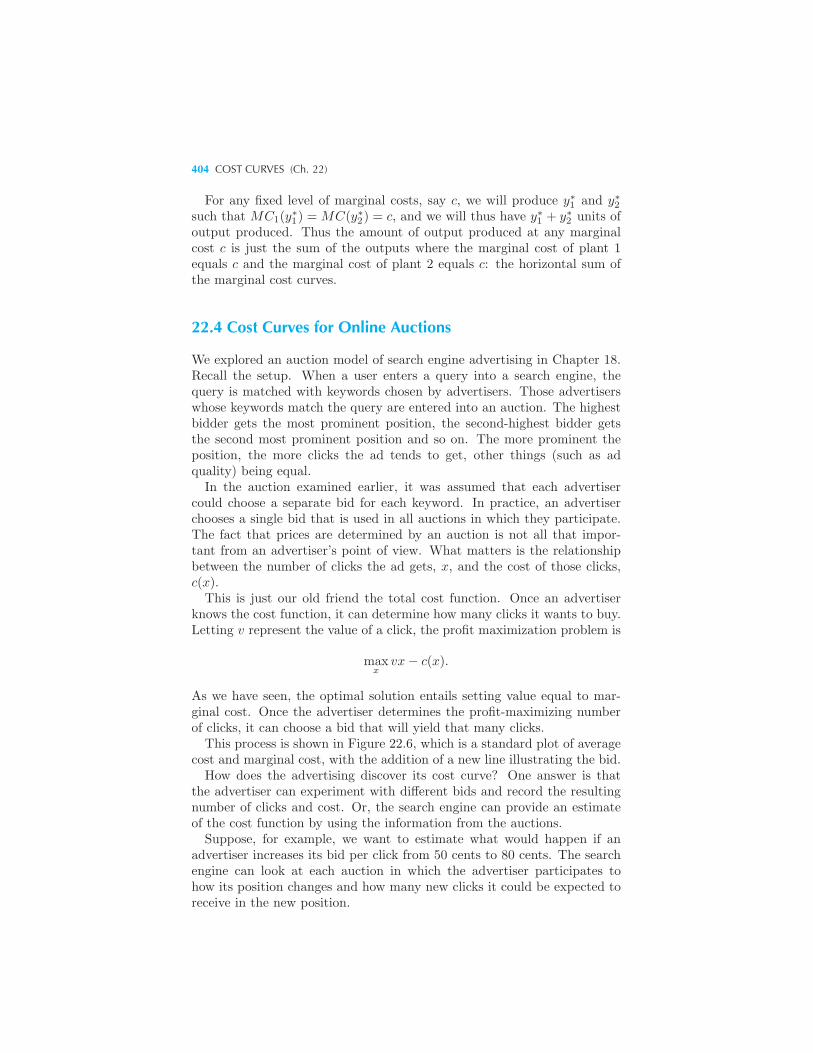
404 COST CURVES (Ch. 22)
For any fixed level of marginal costs, say c, we will produce y∗1 and y∗2such that MC1(y
∗1) = MC(y∗2) = c, and we will thus have y∗1 + y∗2 units of
output produced. Thus the amount of output produced at any marginalcost c is just the sum of the outputs where the marginal cost of plant 1equals c and the marginal cost of plant 2 equals c: the horizontal sum ofthe marginal cost curves.
22.4 Cost Curves for Online Auctions
We explored an auction model of search engine advertising in Chapter 18.Recall the setup. When a user enters a query into a search engine, thequery is matched with keywords chosen by advertisers. Those advertiserswhose keywords match the query are entered into an auction. The highestbidder gets the most prominent position, the second-highest bidder getsthe second most prominent position and so on. The more prominent theposition, the more clicks the ad tends to get, other things (such as adquality) being equal.In the auction examined earlier, it was assumed that each advertiser
could choose a separate bid for each keyword. In practice, an advertiserchooses a single bid that is used in all auctions in which they participate.The fact that prices are determined by an auction is not all that impor-tant from an advertiser’s point of view. What matters is the relationshipbetween the number of clicks the ad gets, x, and the cost of those clicks,c(x).This is just our old friend the total cost function. Once an advertiser
knows the cost function, it can determine how many clicks it wants to buy.Letting v represent the value of a click, the profit maximization problem is
maxx
vx− c(x).
As we have seen, the optimal solution entails setting value equal to mar-ginal cost. Once the advertiser determines the profit-maximizing numberof clicks, it can choose a bid that will yield that many clicks.This process is shown in Figure 22.6, which is a standard plot of average
cost and marginal cost, with the addition of a new line illustrating the bid.How does the advertising discover its cost curve? One answer is that
the advertiser can experiment with different bids and record the resultingnumber of clicks and cost. Or, the search engine can provide an estimateof the cost function by using the information from the auctions.Suppose, for example, we want to estimate what would happen if an
advertiser increases its bid per click from 50 cents to 80 cents. The searchengine can look at each auction in which the advertiser participates tohow its position changes and how many new clicks it could be expected toreceive in the new position.
LONG-RUN COSTS 405
AC
CLICKS
bid(x*)
v = MC(x*)
AC(x*)
x*
Click-cost curves. The profit-maximizing number of clicks iswhere value equals marginal cost, which determines the appro-priate bid and average cost per click.
Figure22.6
22.5 Long-Run Costs
In the above analysis, we have regarded the firm’s fixed costs as being thecosts that involve payments to factors that it is unable to adjust in the shortrun. In the long run a firm can choose the level of its “fixed” factors—theyare no longer fixed.Of course, there may still be quasi-fixed factors in the long run. That
is, it may be a feature of the technology that some costs have to be paidto produce any positive level of output. But in the long run there are nofixed costs, in the sense that it is always possible to produce zero units ofoutput at zero costs—that is, it is always possible to go out of business. Ifquasi-fixed factors are present in the long run, then the average cost curvewill tend to have a U-shape, just as in the short run. But in the long runit will always be possible to produce zero units of output at a zero cost, bydefinition of the long run.Of course, what constitutes the long run depends on the problem we are
analyzing. If we are considering the fixed factor to be the size of the plant,then the long run will be how long it would take the firm to change thesize of its plant. If we are considering the fixed factor to be the contractualobligations to pay salaries, then the long run would be how long it wouldtake the firm to change the size of its work force.Just to be specific, let’s think of the fixed factor as being plant size and
406 COST CURVES (Ch. 22)
denote it by k. The firm’s short-run cost function, given that it has a plantof k square feet, will be denoted by cs(y, k), where the s subscript standsfor “short run.” (Here k is playing the role of x2 in Chapter 21.)For any given level of output, there will be some plant size that is the
optimal size to produce that level of output. Let us denote this plant sizeby k(y). This is the firm’s conditional factor demand for plant size as afunction of output. (Of course, it also depends on the prices of plant sizeand other factors of production, but we have suppressed these arguments.)Then, as we’ve seen in Chapter 21, the long-run cost function of the firmwill be given by cs(y, k(y)). This is the total cost of producing an outputlevel y, given that the firm is allowed to adjust its plant size optimally.The long-run cost function of the firm is just the short-run cost functionevaluated at the optimal choice of the fixed factors:
c(y) = cs(y, k(y)).
Let us see how this looks graphically. Pick some level of output y∗, andlet k∗ = k(y∗) be the optimal plant size for that level of output. The short-run cost function for a plant of size k∗ will be given by cs(y, k
∗), and thelong-run cost function will be given by c(y) = cs(y, k(y)), just as above.
Now, note the important fact that the short-run cost to produce outputy must always be at least as large as the long-run cost to produce y. Why?In the short run the firm has a fixed plant size, while in the long run thefirm is free to adjust its plant size. Since one of its long-run choices isalways to choose the plant size k∗, its optimal choice to produce y units ofoutput must have costs at least as small as c(y, k∗). This means that thefirm must be able to do at least as well by adjusting plant size as by havingit fixed. Thus
c(y) ≤ cs(y, k∗)
for all levels of y.In fact, at one particular level of y, namely y∗, we know that
c(y∗) = cs(y∗, k∗).
Why? Because at y∗ the optimal choice of plant size is k∗. So at y∗, thelong-run costs and the short-run costs are the same.If the short-run cost is always greater than the long-run cost and they
are equal at one level of output, then this means that the short-run and thelong-run average costs have the same property: AC(y) ≤ ACs(y, k
∗) andAC(y∗) = ACs(y
∗, k∗). This implies that the short-run average cost curvealways lies above the long-run average cost curve and that they touch atone point, y∗. Thus the long-run average cost curve (LAC) and the short-run average cost curve (SAC) must be tangent at that point, as depictedin Figure 22.7.
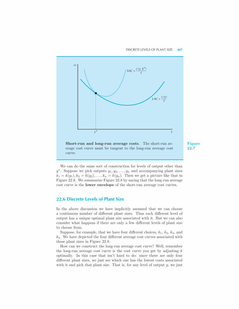
DISCRETE LEVELS OF PLANT SIZE 407
AC
SAC =c (y, k*)
y
LAC =c (y)
y
yy*
Short-run and long-run average costs. The short-run av-erage cost curve must be tangent to the long-run average costcurve.
Figure22.7
We can do the same sort of construction for levels of output other thany∗. Suppose we pick outputs y1, y2, . . . , yn and accompanying plant sizesk1 = k(y1), k2 = k(y2), . . . , kn = k(yn). Then we get a picture like that inFigure 22.8. We summarize Figure 22.8 by saying that the long-run averagecost curve is the lower envelope of the short-run average cost curves.
22.6 Discrete Levels of Plant Size
In the above discussion we have implicitly assumed that we can choosea continuous number of different plant sizes. Thus each different level ofoutput has a unique optimal plant size associated with it. But we can alsoconsider what happens if there are only a few different levels of plant sizeto choose from.Suppose, for example, that we have four different choices, k1, k2, k3, and
k4. We have depicted the four different average cost curves associated withthese plant sizes in Figure 22.9.How can we construct the long-run average cost curve? Well, remember
the long-run average cost curve is the cost curve you get by adjusting koptimally. In this case that isn’t hard to do: since there are only fourdifferent plant sizes, we just see which one has the lowest costs associatedwith it and pick that plant size. That is, for any level of output y, we just
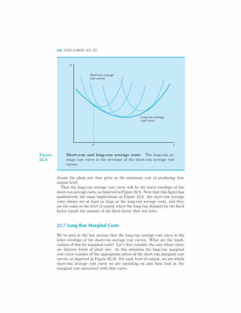
408 COST CURVES (Ch. 22)
Short-run averagecost curves
Long-run averagecost curve
AC
y* y
Figure22.8
Short-run and long-run average costs. The long-run av-erage cost curve is the envelope of the short-run average costcurves.
choose the plant size that gives us the minimum cost of producing thatoutput level.Thus the long-run average cost curve will be the lower envelope of the
short-run average costs, as depicted in Figure 22.9. Note that this figure hasqualitatively the same implications as Figure 22.8: the short-run averagecosts always are at least as large as the long-run average costs, and theyare the same at the level of output where the long-run demand for the fixedfactor equals the amount of the fixed factor that you have.
22.7 Long-Run Marginal Costs
We’ve seen in the last section that the long-run average cost curve is thelower envelope of the short-run average cost curves. What are the impli-cations of this for marginal costs? Let’s first consider the case where thereare discrete levels of plant size. In this situation the long-run marginalcost curve consists of the appropriate pieces of the short-run marginal costcurves, as depicted in Figure 22.10. For each level of output, we see whichshort-run average cost curve we are operating on and then look at themarginal cost associated with that curve.
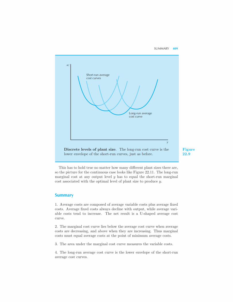
SUMMARY 409
Short-run averagecost curves
Long-run averagecost curve
AC
y
Discrete levels of plant size. The long-run cost curve is thelower envelope of the short-run curves, just as before.
Figure22.9
This has to hold true no matter how many different plant sizes there are,so the picture for the continuous case looks like Figure 22.11. The long-runmarginal cost at any output level y has to equal the short-run marginalcost associated with the optimal level of plant size to produce y.
Summary
1. Average costs are composed of average variable costs plus average fixedcosts. Average fixed costs always decline with output, while average vari-able costs tend to increase. The net result is a U-shaped average costcurve.
2. The marginal cost curve lies below the average cost curve when averagecosts are decreasing, and above when they are increasing. Thus marginalcosts must equal average costs at the point of minimum average costs.
3. The area under the marginal cost curve measures the variable costs.
4. The long-run average cost curve is the lower envelope of the short-runaverage cost curves.
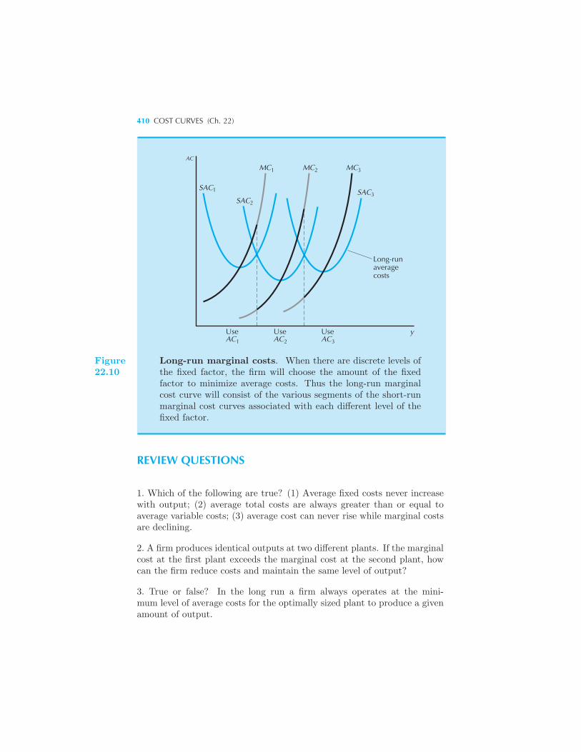
410 COST CURVES (Ch. 22)
2
AC
SAC1
SAC2
SAC3
MC3MCMC1
Long-runaveragecosts
yUseAC2 3
UseAC1
UseAC
Figure22.10
Long-run marginal costs. When there are discrete levels ofthe fixed factor, the firm will choose the amount of the fixedfactor to minimize average costs. Thus the long-run marginalcost curve will consist of the various segments of the short-runmarginal cost curves associated with each different level of thefixed factor.
REVIEW QUESTIONS
1. Which of the following are true? (1) Average fixed costs never increasewith output; (2) average total costs are always greater than or equal toaverage variable costs; (3) average cost can never rise while marginal costsare declining.
2. A firm produces identical outputs at two different plants. If the marginalcost at the first plant exceeds the marginal cost at the second plant, howcan the firm reduce costs and maintain the same level of output?
3. True or false? In the long run a firm always operates at the mini-mum level of average costs for the optimally sized plant to produce a givenamount of output.
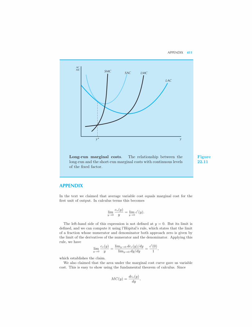
APPENDIX 411
y* y
LAC
LMCSACSMCACMC
Long-run marginal costs. The relationship between thelong-run and the short-run marginal costs with continuous levelsof the fixed factor.
Figure22.11
APPENDIX
In the text we claimed that average variable cost equals marginal cost for thefirst unit of output. In calculus terms this becomes
limy→0
cv(y)
y= lim
y→0c′(y).
The left-hand side of this expression is not defined at y = 0. But its limit isdefined, and we can compute it using l’Hopital’s rule, which states that the limitof a fraction whose numerator and denominator both approach zero is given bythe limit of the derivatives of the numerator and the denominator. Applying thisrule, we have
limy→0
cv(y)
y=
limy→0 dcv(y)/dy
limy→0 dy/dy=
c′(0)
1,
which establishes the claim.We also claimed that the area under the marginal cost curve gave us variable
cost. This is easy to show using the fundamental theorem of calculus. Since
MC(y) =dcv(y)
dy,
412 COST CURVES (Ch. 22)
we know that the area under the marginal cost curve is
cv(y) =
∫ y
0
dcv(x)
dxdx = cv(y)− cv(0) = cv(y).
The discussion of long-run and short-run marginal cost curves is all pretty cleargeometrically, but what does it mean economically? It turns out that the calculusargument gives the nicest intuition. The argument is simple. The marginal costof production is just the change in cost that arises from changing output. In theshort run we have to keep plant size (or whatever) fixed, while in the long runwe are free to adjust it. So the long-run marginal cost will consist of two pieces:how costs change holding plant size fixed plus how costs change when plant sizeadjusts. But if the plant size is chosen optimally, this last term has to be zero!Thus the long-run and the short-run marginal costs have to be the same.
The mathematical proof involves the chain rule. Using the definition from thetext:
c(y) ≡ cs(y, k(y)).
Differentiating with respect to y gives
dc(y)
dy=
∂cs(y, k)
∂y+
∂cs(y, k)
∂k
∂k(y)
∂y.
If we evaluate this at a specific level of output y∗ and its associated optimalplant size k∗ = k(y∗), we know that
∂cs(y∗, k∗)
∂k= 0
because that is the necessary first-order condition for k∗ to be the cost-minimizingplant size at y∗. Thus the second term in the expression cancels out and all thatwe have left is the short-run marginal cost:
dc(y∗)
dy=
∂cs(y∗, k∗)
∂y.

CHAPTER 23
FIRMSUPPLY
In this chapter we will see how to derive the supply curve of a competitivefirm from its cost function using the model of profit maximization. Thefirst thing we have to do is to describe the market environment in whichthe firm operates.
23.1 Market Environments
Every firm faces two important decisions: choosing how much it should pro-duce and choosing what price it should set. If there were no constraints ona profit-maximizing firm, it would set an arbitrarily high price and producean arbitrarily large amount of output. But no firm exists in such an un-constrained environment. In general, the firm faces two sorts of constraintson its actions.First, it faces the technological constraints summarized by the pro-
duction function. There are only certain feasible combinations of inputsand outputs, and even the most profit-hungry firm has to respect the re-alities of the physical world. We have already discussed how we can sum-marize the technological constraints, and we’ve seen how the technological
414 FIRM SUPPLY (Ch. 23)
constraints lead to the economic constraints summarized by the costfunction.But now we bring in a new constraint—or at least an old constraint
from a different perspective. This is the market constraint. A firm canproduce whatever is physically feasible, and it can set whatever price itwants . . . but it can only sell as much as people are willing to buy.If it sets a certain price p it will sell a certain amount of output x. We
call the relationship between the price a firm sets and the amount that itsells the demand curve facing the firm.If there were only one firm in the market, the demand curve facing the
firm would be very simple to describe: it is just the market demand curvedescribed in earlier chapters on consumer behavior. For the market demandcurve measures how much of the good people want to buy at each price.Thus the demand curve summarizes the market constraints facing a firmthat has a market all to itself.But if there are other firms in the market, the constraints facing an
individual firm will be different. In this case, the firm has to guess how theother firms in the market will behave when it chooses its price and output.This is not an easy problem to solve, either for firms or for economists.
There are a lot of different possibilities, and we will try to examine themin a systematic way. We’ll use the term market environment to describethe ways that firms respond to each other when they make their pricingand output decisions.In this chapter we’ll examine the simplest market environment, that
of pure competition. This is a good comparison point for many otherenvironments, and it is of considerable interest in its own right. First let’sgive the economist’s definition of pure competition, and then we’ll try tojustify it.
23.2 Pure Competition
To a lay person, “competition” has the connotation of intense rivalry.That’s why students are often surprised that the economist’s definitionof competition seems so passive: we say that a market is purely compet-itive if each firm assumes that the market price is independent of its ownlevel of output. Thus, in a competitive market, each firm only has to worryabout how much output it wants to produce. Whatever it produces canonly be sold at one price: the going market price.In what sort of environment might this be a reasonable assumption for a
firm to make? Well, suppose that we have an industry composed of manyfirms that produce an identical product, and that each firm is a small partof the market. A good example would be the market for wheat. Thereare thousands of wheat farmers in the United States, and even the largestof them produces only an infinitesimal fraction of the total supply. It is
PURE COMPETITION 415
reasonable in this case for any one firm in the industry to take the marketprice as being predetermined. A wheat farmer doesn’t have to worry aboutwhat price to set for his wheat—if he wants to sell any at all, he has to sellit at the market price. He is a price taker: the price is given as far as heis concerned; all he has to worry about is how much to produce.This kind of situation—an identical product and many small firms—is a
classic example of a situation where price-taking behavior is sensible. Butit is not the only case where price-taking behavior is possible. Even if thereare only a few firms in the market, they may still treat the market price asbeing outside their control.Think of a case where there is a fixed supply of a perishable good: say
fresh fish or cut flowers in a marketplace. Even if there are only 3 or 4firms in the market, each firm may have to take the other firms’ prices asgiven. If the customers in the market only buy at the lowest price, thenthe lowest price being offered is the market price. If one of the other firmswants to sell anything at all, it will have to sell at the market price. Soin this sort of situation competitive behavior—taking the market price asoutside of your control—seems plausible as well.We can describe the relationship between price and quantity perceived
by a competitive firm in terms of a diagram as in Figure 23.1. As you cansee, this demand curve is very simple. A competitive firm believes that itwill sell nothing if it charges a price higher than the market price. If it sellsat the market price, it can sell whatever amount it wants, and if it sellsbelow the market price, it will get the entire market demand at that price.As usual we can think of this kind of demand curve in two ways. If we
think of quantity as a function of price, this curve says that you can sellany amount you want at or below the market price. If we think of priceas a function of quantity, it says that no matter how much you sell, themarket price will be independent of your sales.(Of course, this doesn’t have to be true for literally any amount. Price
has to be independent of your output for any amount you might considerselling. In the case of the cut-flower seller, the price has to be indepen-dent of how much she sells for any amount up to her stock on hand—themaximum that she could consider selling.)It is important to understand the difference between the “demand curve
facing a firm” and the “market demand curve.” The market demand curvemeasures the relationship between the market price and the total amountof output sold. The demand curve facing a firm measures the relationshipbetween the market price and the output of that particular firm.The market demand curve depends on consumers’ behavior. The demand
curve facing a firm not only depends on consumers’ behavior but it alsodepends on the behavior of the other firms. The usual justification for thecompetitive model is that when there are many small firms in the market,each one faces a demand curve that is essentially flat. But even if thereare only two firms in the market, and one insists on charging a fixed price
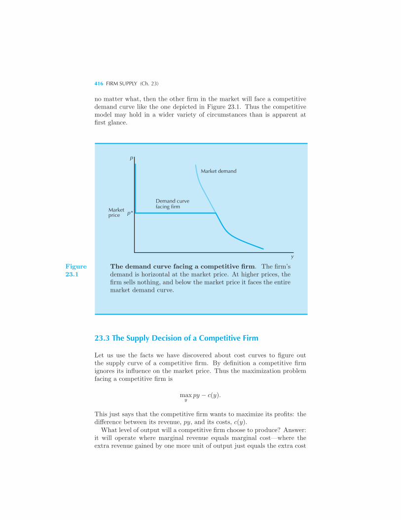
416 FIRM SUPPLY (Ch. 23)
no matter what, then the other firm in the market will face a competitivedemand curve like the one depicted in Figure 23.1. Thus the competitivemodel may hold in a wider variety of circumstances than is apparent atfirst glance.
p
p*Marketprice
Demand curvefacing firm
Market demand
y
Figure23.1
The demand curve facing a competitive firm. The firm’sdemand is horizontal at the market price. At higher prices, thefirm sells nothing, and below the market price it faces the entiremarket demand curve.
23.3 The Supply Decision of a Competitive Firm
Let us use the facts we have discovered about cost curves to figure outthe supply curve of a competitive firm. By definition a competitive firmignores its influence on the market price. Thus the maximization problemfacing a competitive firm is
maxy
py − c(y).
This just says that the competitive firm wants to maximize its profits: thedifference between its revenue, py, and its costs, c(y).
What level of output will a competitive firm choose to produce? Answer:it will operate where marginal revenue equals marginal cost—where theextra revenue gained by one more unit of output just equals the extra cost
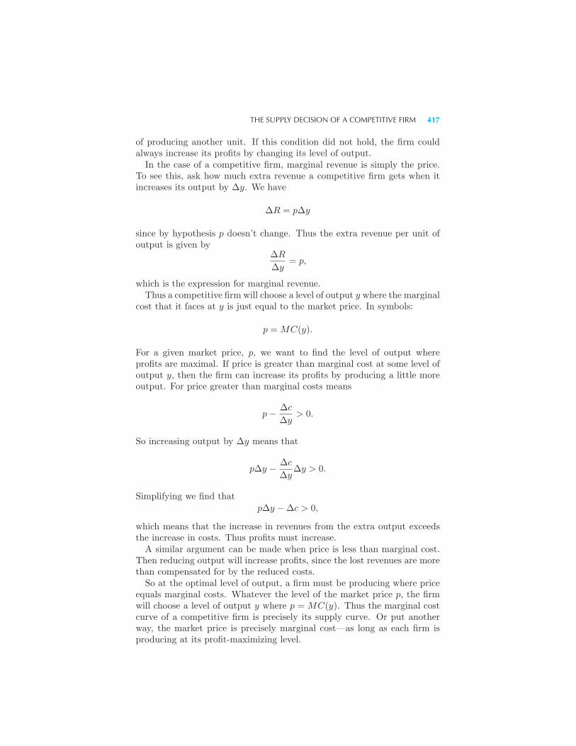
THE SUPPLY DECISION OF A COMPETITIVE FIRM 417
of producing another unit. If this condition did not hold, the firm couldalways increase its profits by changing its level of output.In the case of a competitive firm, marginal revenue is simply the price.
To see this, ask how much extra revenue a competitive firm gets when itincreases its output by Δy. We have
ΔR = pΔy
since by hypothesis p doesn’t change. Thus the extra revenue per unit ofoutput is given by
ΔR
Δy= p,
which is the expression for marginal revenue.Thus a competitive firm will choose a level of output y where the marginal
cost that it faces at y is just equal to the market price. In symbols:
p = MC(y).
For a given market price, p, we want to find the level of output whereprofits are maximal. If price is greater than marginal cost at some level ofoutput y, then the firm can increase its profits by producing a little moreoutput. For price greater than marginal costs means
p− Δc
Δy> 0.
So increasing output by Δy means that
pΔy − Δc
ΔyΔy > 0.
Simplifying we find that
pΔy −Δc > 0,
which means that the increase in revenues from the extra output exceedsthe increase in costs. Thus profits must increase.A similar argument can be made when price is less than marginal cost.
Then reducing output will increase profits, since the lost revenues are morethan compensated for by the reduced costs.So at the optimal level of output, a firm must be producing where price
equals marginal costs. Whatever the level of the market price p, the firmwill choose a level of output y where p = MC(y). Thus the marginal costcurve of a competitive firm is precisely its supply curve. Or put anotherway, the market price is precisely marginal cost—as long as each firm isproducing at its profit-maximizing level.
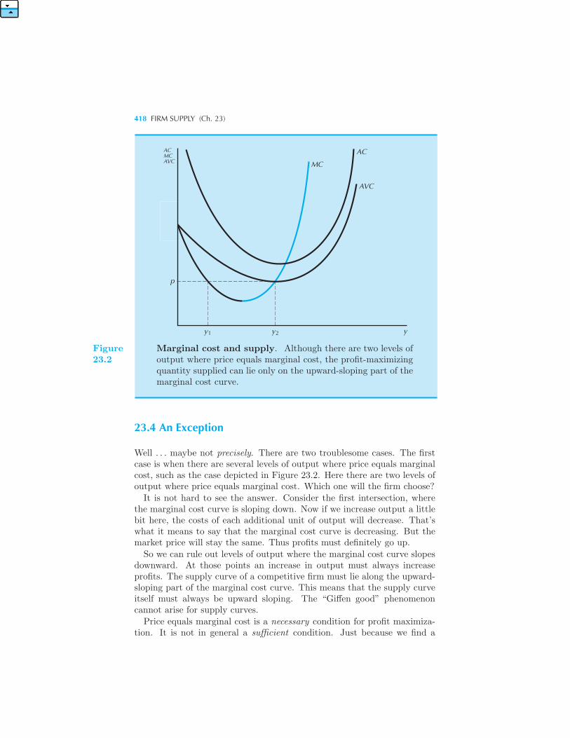
418 FIRM SUPPLY (Ch. 23)
ACMCAVC MC
AC
AVC
y
p
y1 y2
Figure23.2
Marginal cost and supply. Although there are two levels ofoutput where price equals marginal cost, the profit-maximizingquantity supplied can lie only on the upward-sloping part of themarginal cost curve.
23.4 An Exception
Well . . . maybe not precisely. There are two troublesome cases. The firstcase is when there are several levels of output where price equals marginalcost, such as the case depicted in Figure 23.2. Here there are two levels ofoutput where price equals marginal cost. Which one will the firm choose?
It is not hard to see the answer. Consider the first intersection, wherethe marginal cost curve is sloping down. Now if we increase output a littlebit here, the costs of each additional unit of output will decrease. That’swhat it means to say that the marginal cost curve is decreasing. But themarket price will stay the same. Thus profits must definitely go up.
So we can rule out levels of output where the marginal cost curve slopesdownward. At those points an increase in output must always increaseprofits. The supply curve of a competitive firm must lie along the upward-sloping part of the marginal cost curve. This means that the supply curveitself must always be upward sloping. The “Giffen good” phenomenoncannot arise for supply curves.
Price equals marginal cost is a necessary condition for profit maximiza-tion. It is not in general a sufficient condition. Just because we find a
ANOTHER EXCEPTION 419
point where price equals marginal cost doesn’t mean that we’ve found themaximum profit point. But if we find the maximum profit point, we knowthat price must equal marginal cost.
23.5 Another Exception
This discussion is assuming that it is profitable to produce something.After all it could be that the best thing for a firm to do is to produce zerooutput. Since it is always possible to produce a zero level of output, wehave to compare our candidate for profit maximization with the choice ofdoing nothing at all.If a firm produces zero output it still has to pay its fixed costs, F . Thus
the profits from producing zero units of output are just −F . The profitsfrom producing a level of output y are py − cv(y) − F . The firm is betteroff going out of business when
−F > py − cv(y)− F,
that is, when the “profits” from producing nothing, and just paying thefixed costs, exceed the profits from producing where price equals marginalcost. Rearranging this equation gives us the shutdown condition:
AV C(y) =cv(y)
y> p.
If average variable costs are greater than p, the firm would be better offproducing zero units of output. This makes good sense, since it says thatthe revenues from selling the output y don’t even cover the variable costsof production, cv(y). In this case the firm might as well go out of business.If it produces nothing it will lose its fixed costs, but it would lose even moreif it continued to produce.This discussion indicates that only the portions of the marginal cost
curve that lie above the average variable cost curve are possible points onthe supply curve. If a point where price equals marginal cost is beneaththe average variable cost curve, the firm would optimally choose to producezero units of output.We now have a picture for the supply curve like that in Figure 23.3. The
competitive firm produces along the part of the marginal cost curve thatis upward sloping and lies above the average variable cost curve.
EXAMPLE: Pricing Operating Systems
A computer requires an operating system in order to run, and most hard-ware manufacturers sell their computers with the operating systems already
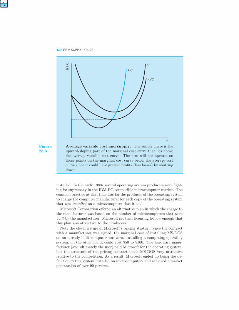
420 FIRM SUPPLY (Ch. 23)
ACAVCMC MC
AC
AVC
y
Figure23.3
Average variable cost and supply. The supply curve is theupward-sloping part of the marginal cost curve that lies abovethe average variable cost curve. The firm will not operate onthose points on the marginal cost curve below the average costcurve since it could have greater profits (less losses) by shuttingdown.
installed. In the early 1980s several operating system producers were fight-ing for supremacy in the IBM-PC-compatible microcomputer market. Thecommon practice at that time was for the producer of the operating systemto charge the computer manufacturer for each copy of the operating systemthat was installed on a microcomputer that it sold.
Microsoft Corporation offered an alternative plan in which the charge tothe manufacturer was based on the number of microcomputers that werebuilt by the manufacturer. Microsoft set their licensing fee low enough thatthis plan was attractive to the producers.
Note the clever nature of Microsoft’s pricing strategy: once the contractwith a manufacturer was signed, the marginal cost of installing MS-DOSon an already-built computer was zero. Installing a competing operatingsystem, on the other hand, could cost $50 to $100. The hardware manu-facturer (and ultimately the user) paid Microsoft for the operating system,but the structure of the pricing contract made MS-DOS very attractiverelative to the competition. As a result, Microsoft ended up being the de-fault operating system installed on microcomputers and achieved a marketpenetration of over 90 percent.
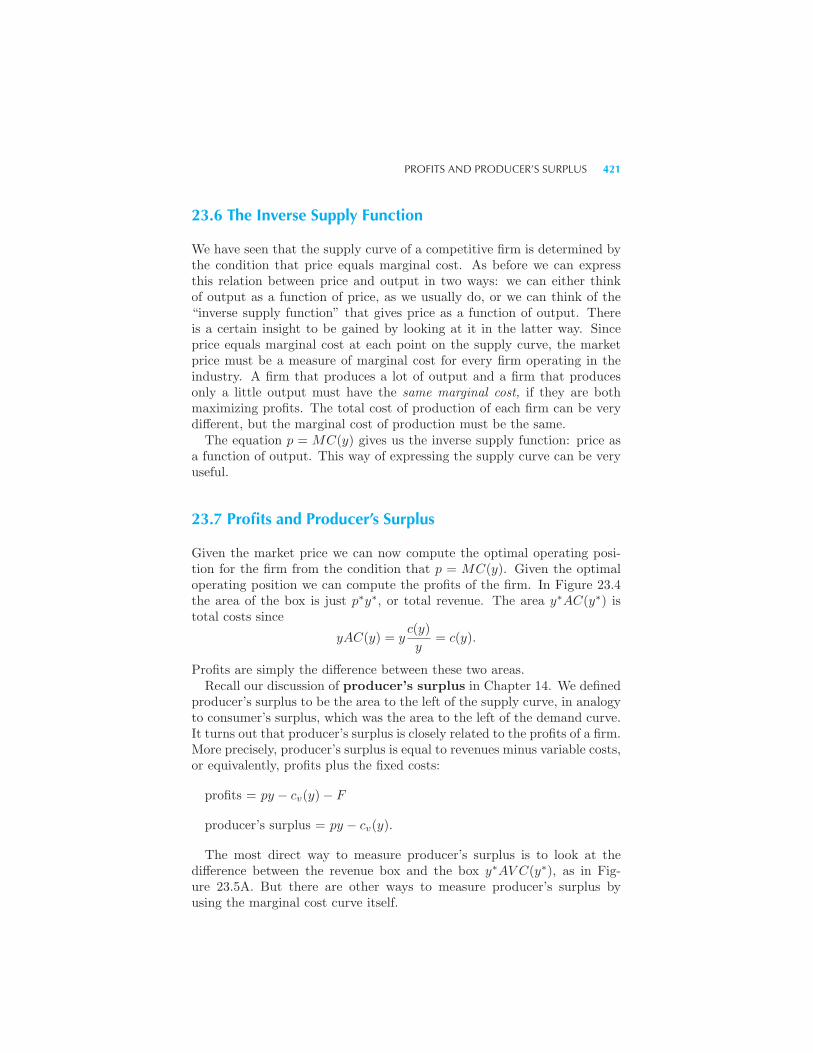
PROFITS AND PRODUCER’S SURPLUS 421
23.6 The Inverse Supply Function
We have seen that the supply curve of a competitive firm is determined bythe condition that price equals marginal cost. As before we can expressthis relation between price and output in two ways: we can either thinkof output as a function of price, as we usually do, or we can think of the“inverse supply function” that gives price as a function of output. Thereis a certain insight to be gained by looking at it in the latter way. Sinceprice equals marginal cost at each point on the supply curve, the marketprice must be a measure of marginal cost for every firm operating in theindustry. A firm that produces a lot of output and a firm that producesonly a little output must have the same marginal cost, if they are bothmaximizing profits. The total cost of production of each firm can be verydifferent, but the marginal cost of production must be the same.The equation p = MC(y) gives us the inverse supply function: price as
a function of output. This way of expressing the supply curve can be veryuseful.
23.7 Profits and Producer’s Surplus
Given the market price we can now compute the optimal operating posi-tion for the firm from the condition that p = MC(y). Given the optimaloperating position we can compute the profits of the firm. In Figure 23.4the area of the box is just p∗y∗, or total revenue. The area y∗AC(y∗) istotal costs since
yAC(y) = yc(y)
y= c(y).
Profits are simply the difference between these two areas.Recall our discussion of producer’s surplus in Chapter 14. We defined
producer’s surplus to be the area to the left of the supply curve, in analogyto consumer’s surplus, which was the area to the left of the demand curve.It turns out that producer’s surplus is closely related to the profits of a firm.More precisely, producer’s surplus is equal to revenues minus variable costs,or equivalently, profits plus the fixed costs:
profits = py − cv(y)− F
producer’s surplus = py − cv(y).
The most direct way to measure producer’s surplus is to look at thedifference between the revenue box and the box y∗AV C(y∗), as in Fig-ure 23.5A. But there are other ways to measure producer’s surplus byusing the marginal cost curve itself.
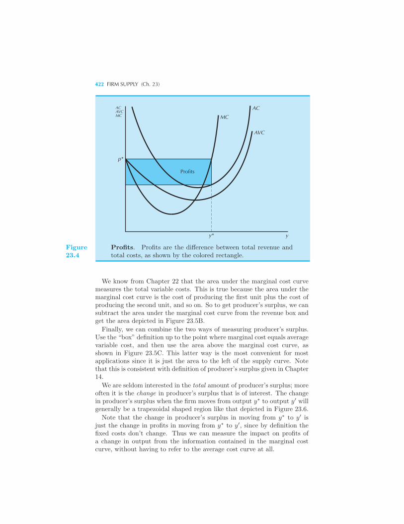
422 FIRM SUPPLY (Ch. 23)
ACAVCMC MC
AC
AVC
yy*
Profits
p*
Figure23.4
Profits. Profits are the difference between total revenue andtotal costs, as shown by the colored rectangle.
We know from Chapter 22 that the area under the marginal cost curvemeasures the total variable costs. This is true because the area under themarginal cost curve is the cost of producing the first unit plus the cost ofproducing the second unit, and so on. So to get producer’s surplus, we cansubtract the area under the marginal cost curve from the revenue box andget the area depicted in Figure 23.5B.
Finally, we can combine the two ways of measuring producer’s surplus.Use the “box” definition up to the point where marginal cost equals averagevariable cost, and then use the area above the marginal cost curve, asshown in Figure 23.5C. This latter way is the most convenient for mostapplications since it is just the area to the left of the supply curve. Notethat this is consistent with definition of producer’s surplus given in Chapter14.
We are seldom interested in the total amount of producer’s surplus; moreoften it is the change in producer’s surplus that is of interest. The changein producer’s surplus when the firm moves from output y∗ to output y′ willgenerally be a trapezoidal shaped region like that depicted in Figure 23.6.
Note that the change in producer’s surplus in moving from y∗ to y′ isjust the change in profits in moving from y∗ to y′, since by definition thefixed costs don’t change. Thus we can measure the impact on profits ofa change in output from the information contained in the marginal costcurve, without having to refer to the average cost curve at all.
PROFITS AND PRODUCER’S SURPLUS 423
ACAVCMC
p
MC = SAC
AVCTR
z y OUTPUT
C Area to the left of the supply curve
ACAVCMC
p
MC = SAC
AVC
z y OUTPUT
A Revenue –variable costs
ACAVCMC
p
MC = SAC
AVC
z y OUTPUT
B Area above MC curve
Producer’s surplus. Three equivalent ways to measure pro-ducer’s surplus. Panel A depicts a box measuring revenue minusvariable cost. Panel B depicts the area above the marginal costcurve. Panel C uses the box up until output z (area R) andthen uses the area above the marginal cost curve (area T ).
Figure23.5
EXAMPLE: The Supply Curve for a Specific Cost Function
What does the supply curve look like for the example given in the lastchapter where c(y) = y2 + 1? In that example the marginal cost curvewas always above the average variable cost curve, and it always slopedupward. So “price equals marginal costs” gives us the supply curve directly.Substituting 2y for marginal cost we get the formula
p = 2y.
This gives us the inverse supply curve, or price as a function of output.Solving for output as a function of price we have
S(p) = y =p
2
as our formula for the supply curve. This is depicted in Figure 23.7.
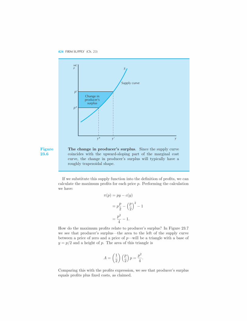
424 FIRM SUPPLY (Ch. 23)
Change inproducer's
surplus
MCp S
p'
y' yy*
p*
Supply curve
Figure23.6
The change in producer’s surplus. Since the supply curvecoincides with the upward-sloping part of the marginal costcurve, the change in producer’s surplus will typically have aroughly trapezoidal shape.
If we substitute this supply function into the definition of profits, we cancalculate the maximum profits for each price p. Performing the calculationwe have:
π(p) = py − c(y)
= pp
2−(p2
)2
− 1
=p2
4− 1.
How do the maximum profits relate to producer’s surplus? In Figure 23.7we see that producer’s surplus—the area to the left of the supply curvebetween a price of zero and a price of p—will be a triangle with a base ofy = p/2 and a height of p. The area of this triangle is
A =
(1
2
)(p2
)p =
p2
4.
Comparing this with the profits expression, we see that producer’s surplusequals profits plus fixed costs, as claimed.
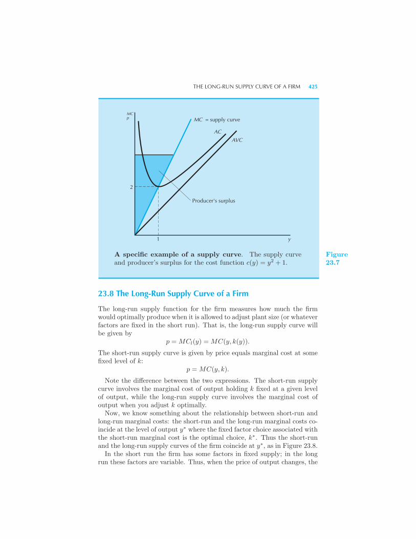
THE LONG-RUN SUPPLY CURVE OF A FIRM 425
MCp MC = supply curve
AC
AVC
Producer's surplus
2
1 y
A specific example of a supply curve. The supply curveand producer’s surplus for the cost function c(y) = y2 + 1.
Figure23.7
23.8 The Long-Run Supply Curve of a Firm
The long-run supply function for the firm measures how much the firmwould optimally produce when it is allowed to adjust plant size (or whateverfactors are fixed in the short run). That is, the long-run supply curve willbe given by
p = MCl(y) = MC(y, k(y)).
The short-run supply curve is given by price equals marginal cost at somefixed level of k:
p = MC(y, k).
Note the difference between the two expressions. The short-run supplycurve involves the marginal cost of output holding k fixed at a given levelof output, while the long-run supply curve involves the marginal cost ofoutput when you adjust k optimally.Now, we know something about the relationship between short-run and
long-run marginal costs: the short-run and the long-run marginal costs co-incide at the level of output y∗ where the fixed factor choice associated withthe short-run marginal cost is the optimal choice, k∗. Thus the short-runand the long-run supply curves of the firm coincide at y∗, as in Figure 23.8.
In the short run the firm has some factors in fixed supply; in the longrun these factors are variable. Thus, when the price of output changes, the
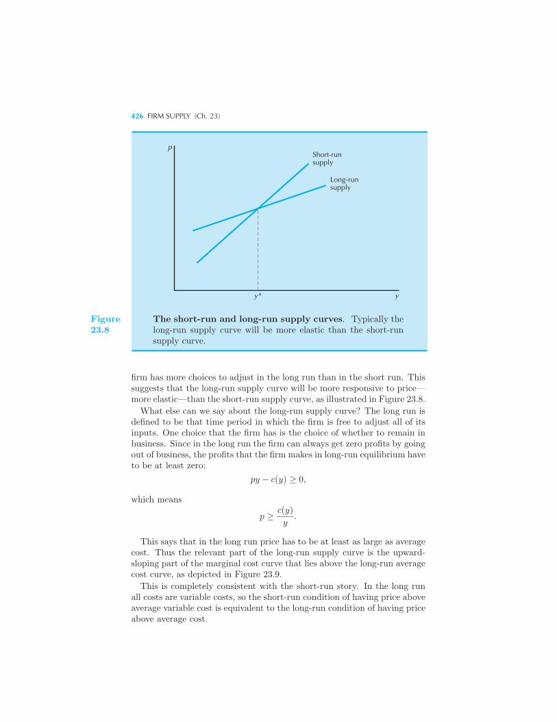
426 FIRM SUPPLY (Ch. 23)
yy*
pShort-runsupply
Long-runsupply
Figure23.8
The short-run and long-run supply curves. Typically thelong-run supply curve will be more elastic than the short-runsupply curve.
firm has more choices to adjust in the long run than in the short run. Thissuggests that the long-run supply curve will be more responsive to price—more elastic—than the short-run supply curve, as illustrated in Figure 23.8.
What else can we say about the long-run supply curve? The long run isdefined to be that time period in which the firm is free to adjust all of itsinputs. One choice that the firm has is the choice of whether to remain inbusiness. Since in the long run the firm can always get zero profits by goingout of business, the profits that the firm makes in long-run equilibrium haveto be at least zero:
py − c(y) ≥ 0,
which means
p ≥ c(y)
y.
This says that in the long run price has to be at least as large as averagecost. Thus the relevant part of the long-run supply curve is the upward-sloping part of the marginal cost curve that lies above the long-run averagecost curve, as depicted in Figure 23.9.
This is completely consistent with the short-run story. In the long runall costs are variable costs, so the short-run condition of having price aboveaverage variable cost is equivalent to the long-run condition of having priceabove average cost.
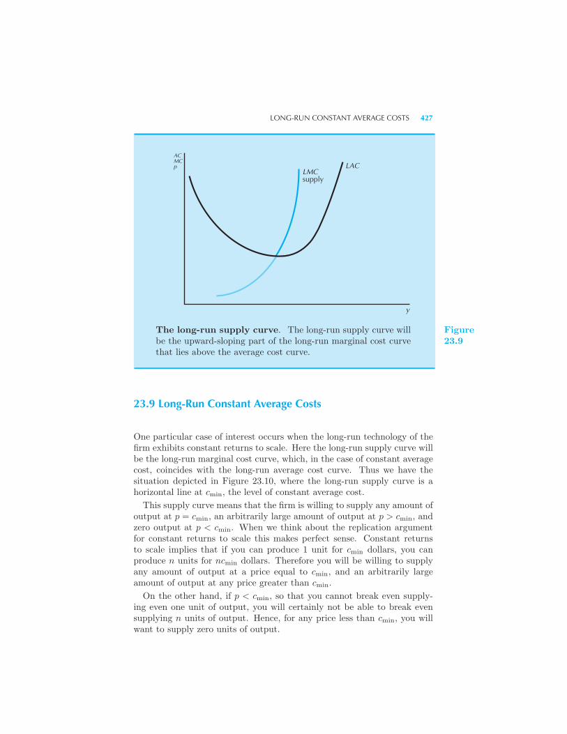
LONG-RUN CONSTANT AVERAGE COSTS 427
ACMCp
LMCsupply
LAC
y
The long-run supply curve. The long-run supply curve willbe the upward-sloping part of the long-run marginal cost curvethat lies above the average cost curve.
Figure23.9
23.9 Long-Run Constant Average Costs
One particular case of interest occurs when the long-run technology of thefirm exhibits constant returns to scale. Here the long-run supply curve willbe the long-run marginal cost curve, which, in the case of constant averagecost, coincides with the long-run average cost curve. Thus we have thesituation depicted in Figure 23.10, where the long-run supply curve is ahorizontal line at cmin, the level of constant average cost.
This supply curve means that the firm is willing to supply any amount ofoutput at p = cmin, an arbitrarily large amount of output at p > cmin, andzero output at p < cmin. When we think about the replication argumentfor constant returns to scale this makes perfect sense. Constant returnsto scale implies that if you can produce 1 unit for cmin dollars, you canproduce n units for ncmin dollars. Therefore you will be willing to supplyany amount of output at a price equal to cmin, and an arbitrarily largeamount of output at any price greater than cmin.
On the other hand, if p < cmin, so that you cannot break even supply-ing even one unit of output, you will certainly not be able to break evensupplying n units of output. Hence, for any price less than cmin, you willwant to supply zero units of output.
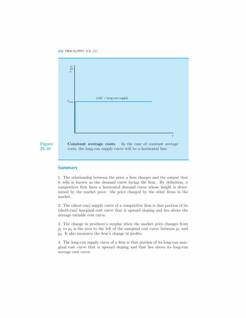
428 FIRM SUPPLY (Ch. 23)
y
ACMCp
Cmin
LMC = long-run supply
Figure23.10
Constant average costs. In the case of constant averagecosts, the long-run supply curve will be a horizontal line.
Summary
1. The relationship between the price a firm charges and the output thatit sells is known as the demand curve facing the firm. By definition, acompetitive firm faces a horizontal demand curve whose height is deter-mined by the market price—the price charged by the other firms in themarket.
2. The (short-run) supply curve of a competitive firm is that portion of its(short-run) marginal cost curve that is upward sloping and lies above theaverage variable cost curve.
3. The change in producer’s surplus when the market price changes fromp1 to p2 is the area to the left of the marginal cost curve between p1 andp2. It also measures the firm’s change in profits.
4. The long-run supply curve of a firm is that portion of its long-run mar-ginal cost curve that is upward sloping and that lies above its long-runaverage cost curve.
APPENDIX 429
REVIEW QUESTIONS
1. A firm has a cost function given by c(y) = 10y2 + 1000. What is itssupply curve?
2. A firm has a cost function given by c(y) = 10y2 +1000. At what outputis average cost minimized?
3. If the supply curve is given by S(p) = 100+20p, what is the formula forthe inverse supply curve?
4. A firm has a supply function given by S(p) = 4p. Its fixed costs are 100.If the price changes from 10 to 20, what is the change in its profits?
5. If the long-run cost function is c(y) = y2+1, what is the long-run supplycurve of the firm?
6. Classify each of the following as either technological or market con-straints: the price of inputs, the number of other firms in the market, thequantity of output produced, and the ability to produce more given thecurrent input levels.
7. What is the major assumption that characterizes a purely competitivemarket?
8. In a purely competitive market a firm’s marginal revenue is always equalto what? A profit-maximizing firm in such a market will operate at whatlevel of output?
9. If average variable costs exceed the market price, what level of outputshould the firm produce? What if there are no fixed costs?
10. Is it ever better for a perfectly competitive firm to produce output eventhough it is losing money? If so, when?
11. In a perfectly competitive market what is the relationship between themarket price and the cost of production for all firms in the industry?
APPENDIX
The discussion in this chapter is very simple if you speak calculus. The profit-maximization problem is
maxy
py − c(y)
such that y ≥ 0.
430 FIRM SUPPLY (Ch. 23)
The necessary conditions for the optimal supply, y∗, are the first-order condition
p− c′(y∗) = 0
and the second-order condition
−c′′(y∗) ≤ 0.
The first-order condition says price equals marginal cost, and the second-ordercondition says that the marginal cost must be increasing. Of course this is pre-suming that y∗ > 0. If price is less than average variable cost at y∗, it will paythe firm to produce a zero level of output. To determine the supply curve of acompetitive firm, we must find all the points where the first- and second-orderconditions are satisfied and compare them to each other—and to y = 0—andpick the one with the largest profits. That’s the profit-maximizing supply.

CHAPTER 24
INDUSTRYSUPPLY
We have seen how to derive a firm’s supply curve from its marginal costcurve. But in a competitive market there will typically be many firms, sothe supply curve the industry presents to the market will be the sum of thesupplies of all the individual firms. In this chapter we will investigate theindustry supply curve.
24.1 Short-Run Industry Supply
We begin by studying an industry with a fixed number of firms, n. We letSi(p) be the supply curve of firm i, so that the industry supply curve,or the market supply curve is
S(p) =
n∑i=1
Si(p),
which is the sum of the individual supply curves. Geometrically we takethe sum of the quantities supplied by each firm at each price, which givesus a horizontal sum of supply curves, as in Figure 24.1.
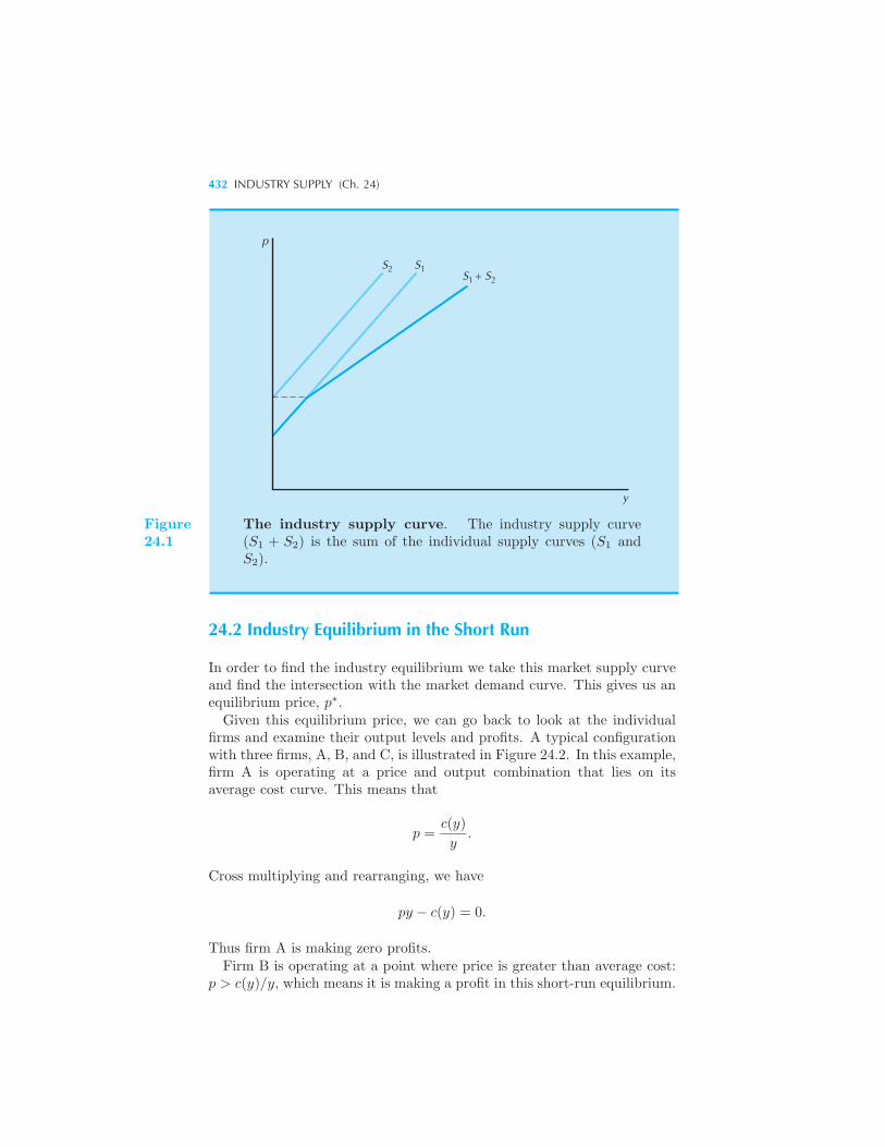
432 INDUSTRY SUPPLY (Ch. 24)
p
S SS + S
y
2 11 2
Figure24.1
The industry supply curve. The industry supply curve(S1 + S2) is the sum of the individual supply curves (S1 andS2).
24.2 Industry Equilibrium in the Short Run
In order to find the industry equilibrium we take this market supply curveand find the intersection with the market demand curve. This gives us anequilibrium price, p∗.
Given this equilibrium price, we can go back to look at the individualfirms and examine their output levels and profits. A typical configurationwith three firms, A, B, and C, is illustrated in Figure 24.2. In this example,firm A is operating at a price and output combination that lies on itsaverage cost curve. This means that
p =c(y)
y.
Cross multiplying and rearranging, we have
py − c(y) = 0.
Thus firm A is making zero profits.Firm B is operating at a point where price is greater than average cost:
p > c(y)/y, which means it is making a profit in this short-run equilibrium.
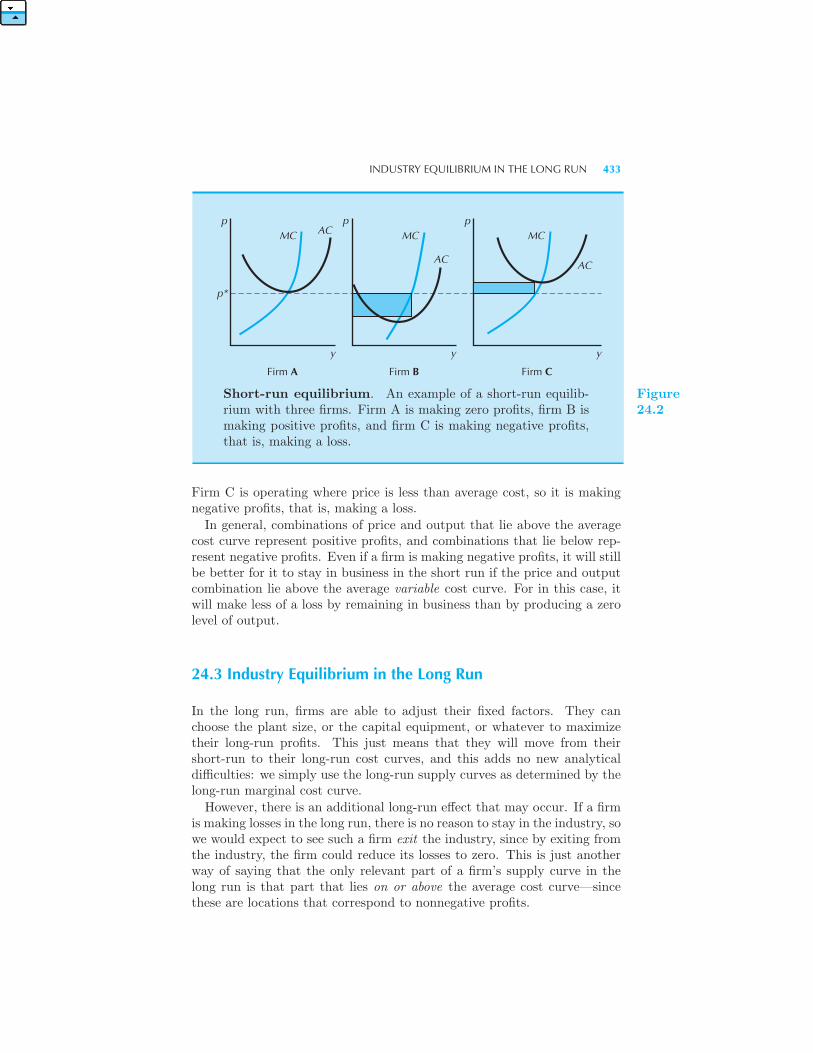
INDUSTRY EQUILIBRIUM IN THE LONG RUN 433
p p pACMC
p*
AC AC
MC MC
y y y
Firm A Firm B Firm C
Short-run equilibrium. An example of a short-run equilib-rium with three firms. Firm A is making zero profits, firm B ismaking positive profits, and firm C is making negative profits,that is, making a loss.
Figure24.2
Firm C is operating where price is less than average cost, so it is makingnegative profits, that is, making a loss.
In general, combinations of price and output that lie above the averagecost curve represent positive profits, and combinations that lie below rep-resent negative profits. Even if a firm is making negative profits, it will stillbe better for it to stay in business in the short run if the price and outputcombination lie above the average variable cost curve. For in this case, itwill make less of a loss by remaining in business than by producing a zerolevel of output.
24.3 Industry Equilibrium in the Long Run
In the long run, firms are able to adjust their fixed factors. They canchoose the plant size, or the capital equipment, or whatever to maximizetheir long-run profits. This just means that they will move from theirshort-run to their long-run cost curves, and this adds no new analyticaldifficulties: we simply use the long-run supply curves as determined by thelong-run marginal cost curve.
However, there is an additional long-run effect that may occur. If a firmis making losses in the long run, there is no reason to stay in the industry, sowe would expect to see such a firm exit the industry, since by exiting fromthe industry, the firm could reduce its losses to zero. This is just anotherway of saying that the only relevant part of a firm’s supply curve in thelong run is that part that lies on or above the average cost curve—sincethese are locations that correspond to nonnegative profits.
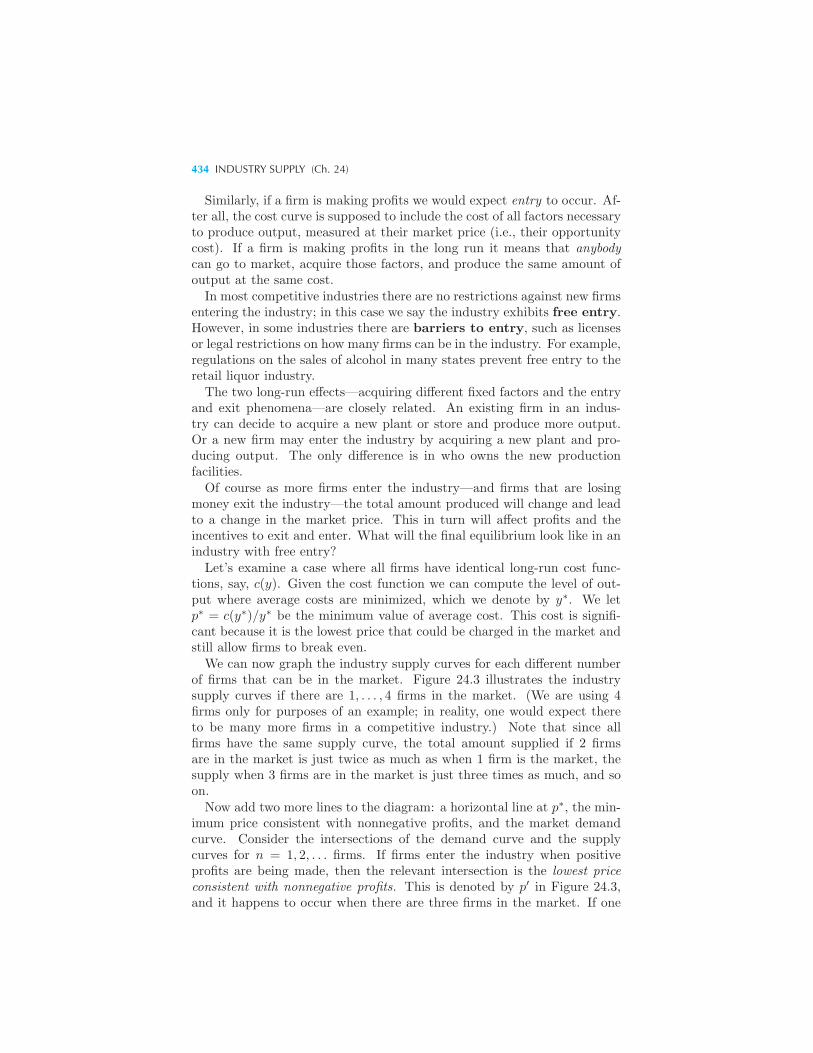
434 INDUSTRY SUPPLY (Ch. 24)
Similarly, if a firm is making profits we would expect entry to occur. Af-ter all, the cost curve is supposed to include the cost of all factors necessaryto produce output, measured at their market price (i.e., their opportunitycost). If a firm is making profits in the long run it means that anybodycan go to market, acquire those factors, and produce the same amount ofoutput at the same cost.In most competitive industries there are no restrictions against new firms
entering the industry; in this case we say the industry exhibits free entry.However, in some industries there are barriers to entry, such as licensesor legal restrictions on how many firms can be in the industry. For example,regulations on the sales of alcohol in many states prevent free entry to theretail liquor industry.The two long-run effects—acquiring different fixed factors and the entry
and exit phenomena—are closely related. An existing firm in an indus-try can decide to acquire a new plant or store and produce more output.Or a new firm may enter the industry by acquiring a new plant and pro-ducing output. The only difference is in who owns the new productionfacilities.Of course as more firms enter the industry—and firms that are losing
money exit the industry—the total amount produced will change and leadto a change in the market price. This in turn will affect profits and theincentives to exit and enter. What will the final equilibrium look like in anindustry with free entry?Let’s examine a case where all firms have identical long-run cost func-
tions, say, c(y). Given the cost function we can compute the level of out-put where average costs are minimized, which we denote by y∗. We letp∗ = c(y∗)/y∗ be the minimum value of average cost. This cost is signifi-cant because it is the lowest price that could be charged in the market andstill allow firms to break even.We can now graph the industry supply curves for each different number
of firms that can be in the market. Figure 24.3 illustrates the industrysupply curves if there are 1, . . . , 4 firms in the market. (We are using 4firms only for purposes of an example; in reality, one would expect thereto be many more firms in a competitive industry.) Note that since allfirms have the same supply curve, the total amount supplied if 2 firmsare in the market is just twice as much as when 1 firm is the market, thesupply when 3 firms are in the market is just three times as much, and soon.Now add two more lines to the diagram: a horizontal line at p∗, the min-
imum price consistent with nonnegative profits, and the market demandcurve. Consider the intersections of the demand curve and the supplycurves for n = 1, 2, . . . firms. If firms enter the industry when positiveprofits are being made, then the relevant intersection is the lowest priceconsistent with nonnegative profits. This is denoted by p′ in Figure 24.3,and it happens to occur when there are three firms in the market. If one
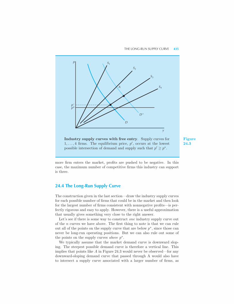
THE LONG-RUN SUPPLY CURVE 435
p
y
A
p'
D''
S3
S4
S1
S2
p*
D
Industry supply curves with free entry. Supply curves for1, . . . , 4 firms. The equilibrium price, p′, occurs at the lowestpossible intersection of demand and supply such that p′ ≥ p∗.
Figure24.3
more firm enters the market, profits are pushed to be negative. In thiscase, the maximum number of competitive firms this industry can supportis three.
24.4 The Long-Run Supply Curve
The construction given in the last section—draw the industry supply curvesfor each possible number of firms that could be in the market and then lookfor the largest number of firms consistent with nonnegative profits—is per-fectly rigorous and easy to apply. However, there is a useful approximationthat usually gives something very close to the right answer.Let’s see if there is some way to construct one industry supply curve out
of the n curves we have above. The first thing to note is that we can ruleout all of the points on the supply curve that are below p∗, since those cannever be long-run operating positions. But we can also rule out some ofthe points on the supply curves above p∗.We typically assume that the market demand curve is downward slop-
ing. The steepest possible demand curve is therefore a vertical line. Thisimplies that points like A in Figure 24.3 would never be observed—for anydownward-sloping demand curve that passed through A would also haveto intersect a supply curve associated with a larger number of firms, as
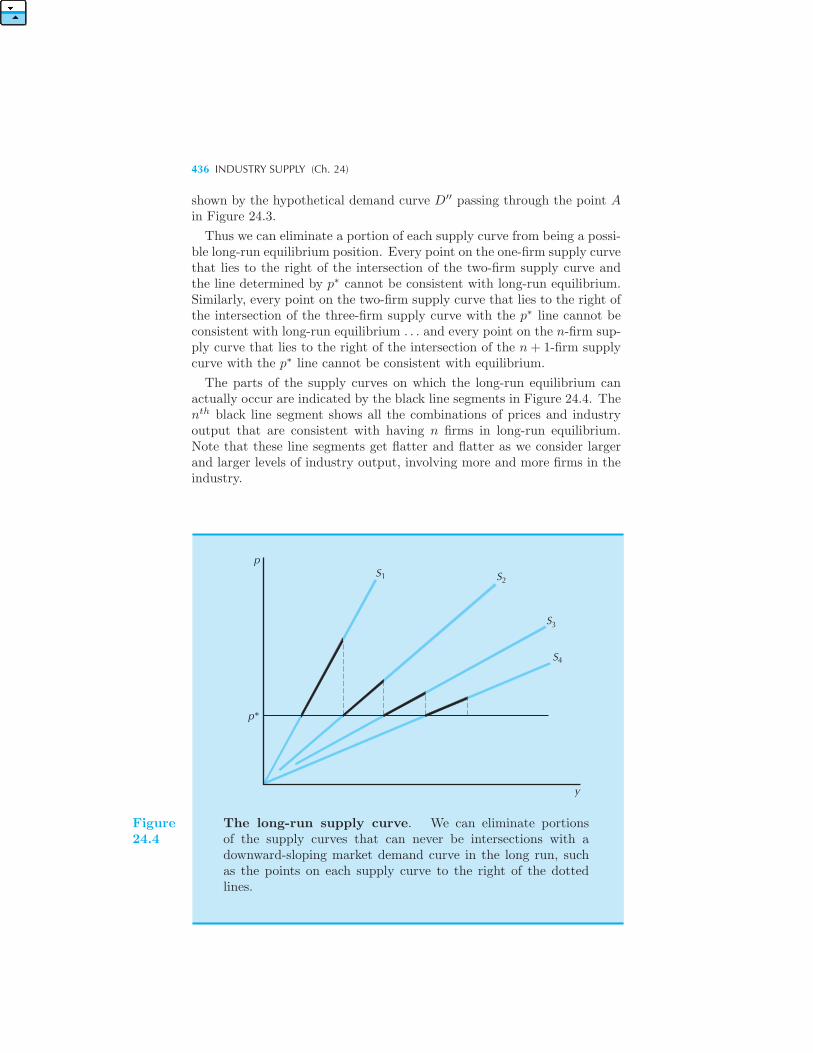
436 INDUSTRY SUPPLY (Ch. 24)
shown by the hypothetical demand curve D′′ passing through the point Ain Figure 24.3.
Thus we can eliminate a portion of each supply curve from being a possi-ble long-run equilibrium position. Every point on the one-firm supply curvethat lies to the right of the intersection of the two-firm supply curve andthe line determined by p∗ cannot be consistent with long-run equilibrium.Similarly, every point on the two-firm supply curve that lies to the right ofthe intersection of the three-firm supply curve with the p∗ line cannot beconsistent with long-run equilibrium . . . and every point on the n-firm sup-ply curve that lies to the right of the intersection of the n+ 1-firm supplycurve with the p∗ line cannot be consistent with equilibrium.
The parts of the supply curves on which the long-run equilibrium canactually occur are indicated by the black line segments in Figure 24.4. Thenth black line segment shows all the combinations of prices and industryoutput that are consistent with having n firms in long-run equilibrium.Note that these line segments get flatter and flatter as we consider largerand larger levels of industry output, involving more and more firms in theindustry.
Sp
p*
S
S
S
2
3
4
1
y
Figure24.4
The long-run supply curve. We can eliminate portionsof the supply curves that can never be intersections with adownward-sloping market demand curve in the long run, suchas the points on each supply curve to the right of the dottedlines.
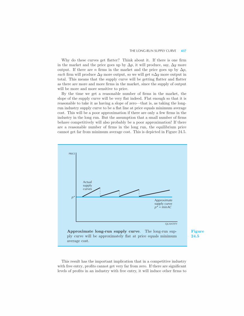
THE LONG-RUN SUPPLY CURVE 437
Why do these curves get flatter? Think about it. If there is one firmin the market and the price goes up by Δp, it will produce, say, Δy moreoutput. If there are n firms in the market and the price goes up by Δp,each firm will produce Δy more output, so we will get nΔy more output intotal. This means that the supply curve will be getting flatter and flatteras there are more and more firms in the market, since the supply of outputwill be more and more sensitive to price.By the time we get a reasonable number of firms in the market, the
slope of the supply curve will be very flat indeed. Flat enough so that it isreasonable to take it as having a slope of zero—that is, as taking the long-run industry supply curve to be a flat line at price equals minimum averagecost. This will be a poor approximation if there are only a few firms in theindustry in the long run. But the assumption that a small number of firmsbehave competitively will also probably be a poor approximation! If thereare a reasonable number of firms in the long run, the equilibrium pricecannot get far from minimum average cost. This is depicted in Figure 24.5.
PRICE
p*
Actualsupplycurves
Approximatesupply curvep* = minAC
QUANTITY
Approximate long-run supply curve. The long-run sup-ply curve will be approximately flat at price equals minimumaverage cost.
Figure24.5
This result has the important implication that in a competitive industrywith free entry, profits cannot get very far from zero. If there are significantlevels of profits in an industry with free entry, it will induce other firms to
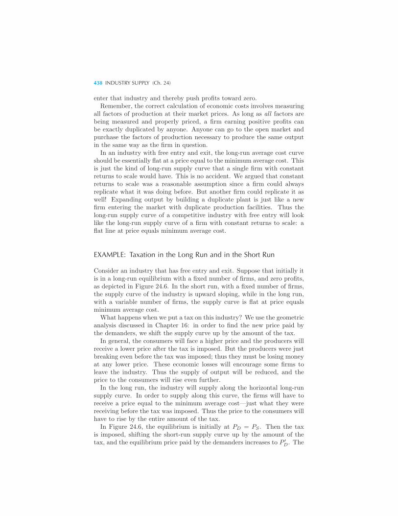
438 INDUSTRY SUPPLY (Ch. 24)
enter that industry and thereby push profits toward zero.Remember, the correct calculation of economic costs involves measuring
all factors of production at their market prices. As long as all factors arebeing measured and properly priced, a firm earning positive profits canbe exactly duplicated by anyone. Anyone can go to the open market andpurchase the factors of production necessary to produce the same outputin the same way as the firm in question.In an industry with free entry and exit, the long-run average cost curve
should be essentially flat at a price equal to the minimum average cost. Thisis just the kind of long-run supply curve that a single firm with constantreturns to scale would have. This is no accident. We argued that constantreturns to scale was a reasonable assumption since a firm could alwaysreplicate what it was doing before. But another firm could replicate it aswell! Expanding output by building a duplicate plant is just like a newfirm entering the market with duplicate production facilities. Thus thelong-run supply curve of a competitive industry with free entry will looklike the long-run supply curve of a firm with constant returns to scale: aflat line at price equals minimum average cost.
EXAMPLE: Taxation in the Long Run and in the Short Run
Consider an industry that has free entry and exit. Suppose that initially itis in a long-run equilibrium with a fixed number of firms, and zero profits,as depicted in Figure 24.6. In the short run, with a fixed number of firms,the supply curve of the industry is upward sloping, while in the long run,with a variable number of firms, the supply curve is flat at price equalsminimum average cost.What happens when we put a tax on this industry? We use the geometric
analysis discussed in Chapter 16: in order to find the new price paid bythe demanders, we shift the supply curve up by the amount of the tax.In general, the consumers will face a higher price and the producers will
receive a lower price after the tax is imposed. But the producers were justbreaking even before the tax was imposed; thus they must be losing moneyat any lower price. These economic losses will encourage some firms toleave the industry. Thus the supply of output will be reduced, and theprice to the consumers will rise even further.In the long run, the industry will supply along the horizontal long-run
supply curve. In order to supply along this curve, the firms will have toreceive a price equal to the minimum average cost—just what they werereceiving before the tax was imposed. Thus the price to the consumers willhave to rise by the entire amount of the tax.In Figure 24.6, the equilibrium is initially at PD = PS . Then the tax
is imposed, shifting the short-run supply curve up by the amount of thetax, and the equilibrium price paid by the demanders increases to P ′
D. The
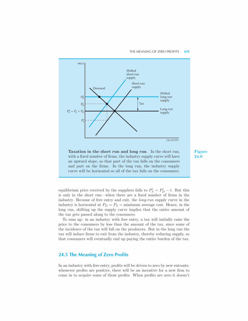
THE MEANING OF ZERO PROFITS 439
D
Demand
Shiftedshort-runsupply
Short-runsupply
Shiftedlong-runsupply
Long-runsupply
Tax
PRICE
QUANTITY
P"
P'
P'
P" = P = P
D
DS S
S
Taxation in the short run and long run. In the short run,with a fixed number of firms, the industry supply curve will havean upward slope, so that part of the tax falls on the consumersand part on the firms. In the long run, the industry supplycurve will be horizontal so all of the tax falls on the consumers.
Figure24.6
equilibrium price received by the suppliers falls to P ′S = P ′
D − t. But thisis only in the short run—when there are a fixed number of firms in theindustry. Because of free entry and exit, the long-run supply curve in theindustry is horizontal at PD = PS = minimum average cost. Hence, in thelong run, shifting up the supply curve implies that the entire amount ofthe tax gets passed along to the consumers.To sum up: in an industry with free entry, a tax will initially raise the
price to the consumers by less than the amount of the tax, since some ofthe incidence of the tax will fall on the producers. But in the long run thetax will induce firms to exit from the industry, thereby reducing supply, sothat consumers will eventually end up paying the entire burden of the tax.
24.5 The Meaning of Zero Profits
In an industry with free entry, profits will be driven to zero by new entrants:whenever profits are positive, there will be an incentive for a new firm tocome in to acquire some of those profits. When profits are zero it doesn’t
440 INDUSTRY SUPPLY (Ch. 24)
mean that the industry disappears; it just means that it stops growing,since there is no longer an inducement to enter.In a long-run equilibrium with zero profits, all of the factors of production
are being paid their market price—the same market price that these factorscould earn elsewhere. The owner of the firm, for example, is still collectinga payment for her labor time, or for the amount of money she investedin the firm, or for whatever she contributes to the operation of the firm.The same goes for all other factors of production. The firm is still makingmoney—it is just that all the money that it makes is being paid out topurchase the inputs that it uses. Each factor of production is earning thesame amount in this industry that it could earn elsewhere, so there areno extra rewards—no pure profits—to attract new factors of production tothis industry. But there is nothing to cause them to leave either. Industriesin long-run equilibrium with zero profits are mature industries; they’re notlikely to appear as the cover story in Business Week, but they form thebackbone of the economy.Remember, economic profits are defined using the market prices of all
factors of production. The market prices measure the opportunity costof those factors—what they could earn elsewhere. Any amount of moneyearned in excess of the payments to the factors of production is a pureeconomic profit. But whenever someone finds a pure economic profit, otherpeople will try to enter the industry and acquire some of that profit forthemselves. It is this attempt to capture economic profits that eventuallydrives them to zero in a competitive industry with free entry.In some quarters, the profit motive is regarded with some disdain. But
when you think about it purely on economic grounds, profits are providingexactly the right signals as far as resource allocation is concerned. If a firmis making positive profits, it means that people value the output of thefirm more highly than they value the inputs. Doesn’t it make sense to havemore firms producing that kind of output?
24.6 Fixed Factors and Economic Rent
If there is free entry, profits are driven to zero in the long run. But notevery industry has free entry. In some industries the number of firms inthe industry is fixed.A common reason for this is that there are some factors of production
that are available in fixed supply. We said that in the long run the fixedfactors could be bought or sold by an individual firm. But there are somefactors that are fixed for the economy as a whole even in the long run.The most obvious example of this is in resource-extraction industries:
oil in the ground is a necessary input to the oil-extraction industry, andthere is only so much oil around to be extracted. A similar statementcould be made for coal, gas, precious metals, or any other such resource.
FIXED FACTORS AND ECONOMIC RENT 441
Agriculture gives another example. There is only a certain amount of landthat is suitable for agriculture.A more exotic example of such a fixed factor is talent. There are only
a certain number of people who possess the necessary level of talent to beprofessional athletes or entertainers. There may be “free entry” into suchfields—but only for those who are good enough to get in!There are other cases where the fixed factor is fixed not by nature, but
by law. In many industries it is necessary to have a license or permit, andthe number of these permits may be fixed by law. The taxicab industry inmany cities is regulated in this way. Liquor licenses are another example.If there are restrictions such as the above on the number of firms in the
industry, so that firms cannot enter the industry freely, it may appear thatit is possible to have an industry with positive profits in the long run, withno economic forces to drive those profits to zero.This appearance is wrong. There is an economic force that pushes profits
to zero. If a firm is operating at a point where its profits appear to bepositive in the long run, it is probably because we are not appropriatelymeasuring the market value of whatever it is that is preventing entry.Here it is important to remember the economic definition of costs: we
should value each factor of production at its market price—its opportunitycost. If it appears that a farmer is making positive profits after we havesubtracted his costs of production, it is probably because we have forgottento subtract the cost of his land.Suppose that we manage to value all of the inputs to farming except for
the land cost, and we end up with π dollars per year for profits. How muchwould the land be worth on a free market? How much would someone payto rent that land for a year?The answer is: they would be willing to rent it for π dollars per year,
the “profits” that it brings in. You wouldn’t even have to know anythingabout farming to rent this land and earn π dollars—after all, we valuedthe farmer’s labor at its market price as well, and that means that you canhire a farmer and still make π dollars of profit. So the market value of thatland—its competitive rent—is just π. The economic profits to farming arezero.Note that the rental rate determined by this procedure may have nothing
whatsoever to do with the historical cost of the farm. What matters is notwhat you bought it for, but what you can sell it for—that’s what determinesopportunity cost.Whenever there is some fixed factor that is preventing entry into an
industry, there will be an equilibrium rental rate for that factor. Even withfixed factors, you can always enter an industry by buying out the positionof a firm that is currently in the industry. Every firm in the industry hasthe option of selling out—and the opportunity cost of not doing so is a costof production that it has to consider.Thus in one sense it is always the possibility of entry that drives profits to
442 INDUSTRY SUPPLY (Ch. 24)
zero. After all, there are two ways to enter an industry: you can form a newfirm, or you can buy out an existing firm that is currently in the industry.If a new firm can buy everything necessary to produce in an industry andstill make a profit, it will do so. But if there are some factors that are infixed supply, then competition for those factors among potential entrantswill bid the prices of these factors up to a point where the profit disappears.
EXAMPLE: Taxi Licenses in New York City
Earlier we said that licenses to operate New York City taxicabs sell forabout $100,000. Yet in 1986 taxicab drivers made only about $400 for a50-hour week; this translated into less than an $8 hourly wage. The NewYork Taxi and Limosine Commission argued that this wage was too lowto attract skilled drivers and that taxi fares should be raised in order toattract better drivers.An economist would argue that allowing the fares to increase would have
virtually no effect on the take-home pay of the drivers; all that wouldhappen is that the value of the taxicab license would increase. We can seewhy by examining the commission’s figures for the costs of operating a taxi.In 1986, the lease rate was $55 for a day shift and $65 for a night shift.The driver who leased the taxi paid for the gasoline and netted about $80a day in income.But note how much the owner of the taxicab license made. Assuming
that the cab could be rented for two shifts for 320 days a year, the leaseincome comes to $38,400. Insurance, depreciation, maintenance, and so onamounted to about $21,100 a year; this leaves a net profit of $17,300 peryear. Since the license cost about $100,000, this indicates a total return ofabout 17 percent.An increase in the rate that taxis were allowed to charge would be re-
flected directly in the value of the license. A fare increase that broughtin an extra $10,000 a year would result in a license’s value increasing byabout $60,000. The wage rate for the cab drivers—which is set in the labormarket—would not be affected by such a change.1
24.7 Economic Rent
The examples in the last section are instances of economic rent. Eco-nomic rent is defined as those payments to a factor of production that arein excess of the minimum payment necessary to have that factor supplied.
1 Figures are taken from an unsigned editorial in the New York Times, August 17,1986.
ECONOMIC RENT 443
Consider, for example, the case of oil discussed earlier. In order to pro-duce oil you need some labor, some machinery, and, most importantly,some oil in the ground! Suppose that it costs $1 a barrel to pump oil outof the ground from an existing well. Then any price in excess of $1 a barrelwill induce firms to supply oil from existing wells. But the actual price ofoil is much higher than $1 a barrel. People want oil for various reasons,and they are willing to pay more than its cost of production to get it. Theexcess of the price of oil over its cost of production is economic rent.Why don’t firms enter this industry? Well, they try. But there is only
a certain amount of oil available. Oil will sell for more than its cost ofproduction because of the limited supply.Now consider taxicab licenses. Viewed as pieces of paper, these cost
almost nothing to produce. But in New York City a taxicab license cansell for $100,000! Why don’t people enter this industry and produce moretaxicab licenses? The reason is that entry is illegal—the supply of taxicablicenses is controlled by the city.Farmland is yet another example of economic rent. In the aggregate, the
total amount of land is fixed. There would be just as much land suppliedat zero dollars an acre as at $1000 an acre. Thus in the aggregate, thepayments to land constitute economic rent.From the viewpoint of the economy as a whole, it is the price of agri-
cultural products that determines the value of agricultural land. But fromthe viewpoint of the individual farmer, the value of his land is a cost ofproduction that enters into the pricing of his product.This is depicted in Figure 24.7. Here AV C represents the average cost
curve for all factors of production excluding land costs. (We are assumingthat land is the only fixed factor.) If the price of the crop grown on thisland is p∗, then the “profits” attributable to the land are measured bythe area of the box: these are the economic rents. This is how much theland would rent for in a competitive market—whatever it took to drive theprofits to zero.The average cost curve including the value of the land is labeled AC. If
we measure the value of the land correctly, the economic profits to operatingthe farm will be exactly zero. Since the equilibrium rent for the land willbe whatever it takes to drive profits to zero, we have
p∗y∗ − cv(y∗)− rent = 0
or
rent = p∗y∗ − cv(y∗). (24.1)
This is precisely what we referred to as producer’s surplus earlier. Indeed,it is the same concept, simply viewed in a different light. Thus we can alsomeasure rent by taking the area to the left of the marginal cost curve, aswe saw earlier.
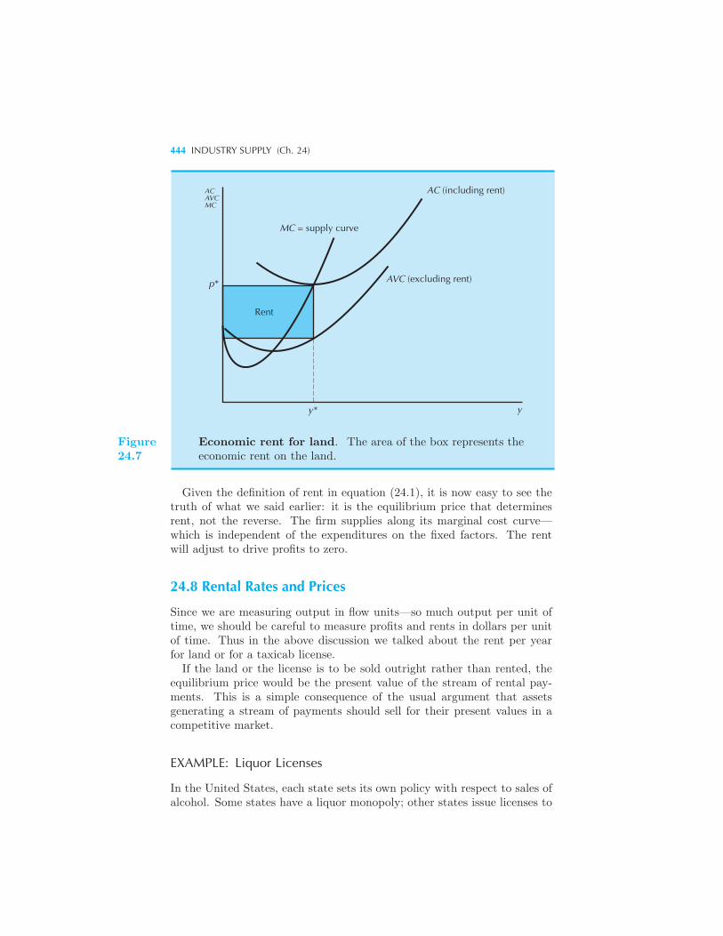
444 INDUSTRY SUPPLY (Ch. 24)
MC = supply curve
AC (including rent)
AVC (excluding rent)
ACAVCMC
yy*
p*
Rent
Figure24.7
Economic rent for land. The area of the box represents theeconomic rent on the land.
Given the definition of rent in equation (24.1), it is now easy to see thetruth of what we said earlier: it is the equilibrium price that determinesrent, not the reverse. The firm supplies along its marginal cost curve—which is independent of the expenditures on the fixed factors. The rentwill adjust to drive profits to zero.
24.8 Rental Rates and Prices
Since we are measuring output in flow units—so much output per unit oftime, we should be careful to measure profits and rents in dollars per unitof time. Thus in the above discussion we talked about the rent per yearfor land or for a taxicab license.If the land or the license is to be sold outright rather than rented, the
equilibrium price would be the present value of the stream of rental pay-ments. This is a simple consequence of the usual argument that assetsgenerating a stream of payments should sell for their present values in acompetitive market.
EXAMPLE: Liquor Licenses
In the United States, each state sets its own policy with respect to sales ofalcohol. Some states have a liquor monopoly; other states issue licenses to
THE POLITICS OF RENT 445
those who wish to sell alcohol. In some cases, licenses are issued on paymentof a fee; in other cases, the number of licenses is fixed. In Michigan, forexample, the number of licenses for sales of beer and wine for consumptionon premises is limited to one for every 1,500 residents.After each Federal census, a state liquor control board allocates licenses
to communities whose populations have grown. (Licenses are not takenaway from communities whose populations have fallen, however.) Thisartificial scarcity of licenses has created a vibrant market for licenses toserve liquor in many fast-growing communities. For example, in 1983 AnnArbor, Michigan, had sixty-six existing liquor licenses. Six new licenseswere allowed to be issued as a result of the 1980 census, and 33 applicantslined up to lobby for these licenses. At the time, the market value of a liquorlicense was about $80,000. The local newspaper ran a story asserting that“demand exceeds supply for liquor licenses.” It was hardly surprising to thelocal economists that giving away an $80,000 asset for a zero price resultedin excess demand!There have been many proposals to relax the liquor control laws in Michi-
gan by allowing the state to issue new licenses. However, these proposalshave never been enacted into law due to the opposition of various politicalgroups. Some of these groups are opposed to the consumption of alcoholon grounds of public health or religion. Others have somewhat differentmotives. For example, one of the most vociferous opponents of relaxedliquor laws is the Michigan Licensed Beverage Association, a group thatrepresents the sellers of alcoholic beverages in Michigan. Though at firstglance it appears paradoxical that this group would oppose liberalizationof the liquor laws, a little reflection indicates a possible reason: issuingmore liquor licenses would undoubtably lower the resale value of existinglicenses—imposing significant capital losses on current holders of such li-censes.
24.9 The Politics of Rent
Often economic rent exists because of legal restrictions on entry into theindustry. We mentioned two examples above: taxicab licenses and liquorlicenses. In each of these cases the number of licenses is fixed by law, thusrestricting entry to the industry and creating economic rents.Suppose that the New York City government wants to increase the num-
ber of operating taxicabs. What will happen to the market value of theexisting taxicab licenses? Obviously they will fall in value. This reductionin value hits the industry right in the pocketbook, and it is sure to createa lobbying force to oppose any such move.The federal government also artificially restricts output of some products
in such a way as to create a rent. For example, the federal government hasdeclared that tobacco can only be grown on certain lands. The value of
446 INDUSTRY SUPPLY (Ch. 24)
this land is then determined by the demand for tobacco products. Anyattempt to eliminate this licensing system has to contend with a seriouslobby. Once the government creates artificial scarcity, it is very hard toeliminate it. The beneficiaries of the artificial scarcity—the people whohave acquired the right to operate in the industry—will vigorously opposeany attempts to enlarge the industry.The incumbents in an industry in which entry is legally restricted may
well devote considerable resources to maintaining their favored position.Lobbying expenses, lawyers’ fees, public relations costs, and so on can besubstantial. From the viewpoint of society these kinds of expenses representpure social waste. They aren’t true costs of production; they don’t leadto any more output being produced. Lobbying and public relations effortsjust determine who gets the money associated with existing output.Efforts directed at keeping or acquiring claims to factors in fixed supplies
are sometimes referred to as rent seeking. From the viewpoint of societythey represent a pure deadweight loss since they don’t create any moreoutput, they just change the market value of existing factors of production.
EXAMPLE: Farming the Government
There is only one good thing to say about the U.S. program of farm sub-sidies: it produces a never-ending source of examples for economics text-books. Every new reform of the farm program brings new problems. “Ifyou want to find the holes in a program, just toss them out to farmers. Noone is more innovative in finding ways to use them,” says Terry Bar, thevice president of the National Council of Farm Cooperatives.2
Up until 1996 the basic structure of farm subsidies in the U.S. involvedprice supports: the Federal government guaranteed a support price for acrop and would make up the difference if the price fell below the supportprice. In order to qualify for this program, a farmer had to agree not tofarm a certain fraction of his land.By the very nature of this plan, most of the benefits accrued to the large
farmers. According to one calculation, 13 percent of the direct Federalsubsidies were going to the 1 percent of the farmers who had sales over$500,000 a year. The Food Security Act of 1985 significantly restricted thepayments to large farmers. As a result, the farmers broke up their holdingsby leasing the land to local investors. The investors would acquire parcelslarge enough to take advantage of the subsidies, but too small to run intothe restrictions aimed at large farmers. Once the land was acquired theinvestor would register it with a government program that would pay the
2 Quoted in William Robbins, “Limits on Subsidies to Big Farms Go Awry, SendingCosts Climbing,” New York Times, June 15, 1987, A1.
ENERGY POLICY 447
investor not to plant the land. This practice became known as “farmingthe government.”According to one study, the restriction on payments to the large farmers
in the 1985 farm act resulted in the creation of 31,000 new applicants forfarm subsidies. The cost of these subsidies was in the neighborhood of $2.3billion.Note that the ostensible goal of the program—restricting the amount of
government subsidies paid to large farmers—has not been achieved. Whenthe large farmers rent their land to small farmers, the market price of therents depends on the generosity of the Federal subsidies. The higher thesubsidies, the higher the equilibrium rent the large farmers receive. Thebenefits from the subsidy program still falls on those who initially ownthe land, since it is ultimately the value of what the land can earn—eitherfrom growing crops or farming the government—that determines its marketvalue.The Farm Act of 1996 promised a phaseout of most agricultural subsidies
by 2002. However, the 1998 federal budget restored over 6 billion dollarsof federal farm subsidies, illustrating once again how hard it is to reconcilepolitics and economics.
24.10 Energy Policy
We end this chapter with an extended example that uses some of the con-cepts we have developed.In 1974 the Organization of Petroleum Exporting Countries (OPEC)
levied a significant increase in the price of oil. Countries that had nodomestically produced petroleum had little choice about energy policy—the price of oil and goods produced using oil had to rise.At that time the United States produced about half of its domestic oil
consumption, and Congress felt that it was unfair that the domestic pro-ducers should receive “windfall profits” from an uncontrolled increase inprice. (The term windfall profits refers to an increase in profits due tosome outside event, as opposed to an increase in profits due to productiondecisions.) Consequently, Congress devised a bizarre plan to attempt tohold down the price of products that used oil. The most prominent ofthese products is gasoline, so we will analyze the effect of the program forthat market.
Two-Tiered Oil Pricing
The policy adopted by Congress was known as “two-tiered” oil pricing,and it went something like this. Imported oil would sell for whatever itsmarket price was, but domestic oil—oil produced from wells that were in
448 INDUSTRY SUPPLY (Ch. 24)
place before 1974—would sell for its old price: the price that it sold forbefore OPEC. Roughly speaking, we’ll say that imported oil sold for about$15 a barrel, while domestic oil sold for around $5. The idea was that theaverage price of oil would then be about $10 a barrel and this would helphold down the price of gasoline.Could such a scheme work? Let’s think about it from the viewpoint of
the gasoline producers. What would the supply curve of gasoline look like?In order to answer this question we have to ask what the marginal costcurve for gasoline looked like.What would you do if you were a gasoline refiner? Obviously you would
try to use the cheap domestic oil first. Only after you had exhausted yoursupplies of domestic oil would you turn to the more expensive imported oil.Thus the aggregate marginal cost curve—the industry supply curve—forgasoline would have to look something like that depicted in Figure 24.8.The curve takes a jump at the point where the U.S. production of domesticoil is exhausted and the imported oil begins to be used. Before that point,the domestic price of oil measures the relevant factor price for producinggasoline. After that point, it is the price of foreign oil that is the relevantfactor price.Figure 24.8 depicts the supply curve for gasoline if all oil were to sell for
the world price of $15 a barrel, and if all oil were to sell for the domesticprice of $5 a barrel. If domestic oil actually sells for $5 a barrel and foreignoil sells for $15 a barrel, then the supply curve for gasoline will coincidewith the $5-a-barrel supply curve until the cheaper domestic oil is used up,and then coincide with the $15-a-barrel supply curve.Now let’s find the intersection of this supply curve with the market de-
mand curve to find the equilibrium price in Figure 24.8. The diagramreveals an interesting fact: the price of gasoline is exactly the same in thetwo-tiered system as it would be if all oil sold at the price of foreign oil!The price of gasoline is determined by the marginal cost of production, andthe marginal cost is determined by the cost of the imported oil.
If you think about it a minute, this makes perfectly good sense. Thegasoline companies will sell their product at the price the market will bear.Just because you were lucky enough to get some cheap oil doesn’t meanyou won’t sell your gasoline for the same price that other firms are sellingtheirs for.Suppose for the moment that all oil did sell for one price, and that
equilibrium was reached at the price p∗. Then the government comes alongand lowers the price of the first 100 barrels of oil that each refiner used.Will this affect their supply decision? No way—in order to affect supplyyou have to change the incentives at the margin. The only way to get alower price of gasoline is to increase the supply, which means that you haveto make the marginal cost of oil cheaper.The two-tiered oil pricing policy was simply a transfer from the domestic
oil producers to the domestic oil refiners. The domestic producers got $10
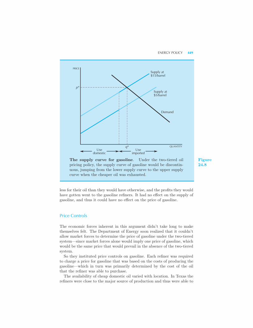
ENERGY POLICY 449
PRICE
p*
q* QUANTITY
Supply at$15/barrel
Supply at$5/barrel
Demand
Usedomestic
Useimported
The supply curve for gasoline. Under the two-tiered oilpricing policy, the supply curve of gasoline would be discontin-uous, jumping from the lower supply curve to the upper supplycurve when the cheaper oil was exhausted.
Figure24.8
less for their oil than they would have otherwise, and the profits they wouldhave gotten went to the gasoline refiners. It had no effect on the supply ofgasoline, and thus it could have no effect on the price of gasoline.
Price Controls
The economic forces inherent in this argument didn’t take long to makethemselves felt. The Department of Energy soon realized that it couldn’tallow market forces to determine the price of gasoline under the two-tieredsystem—since market forces alone would imply one price of gasoline, whichwould be the same price that would prevail in the absence of the two-tieredsystem.So they instituted price controls on gasoline. Each refiner was required
to charge a price for gasoline that was based on the costs of producing thegasoline—which in turn was primarily determined by the cost of the oilthat the refiner was able to purchase.The availability of cheap domestic oil varied with location. In Texas the
refiners were close to the major source of production and thus were able to
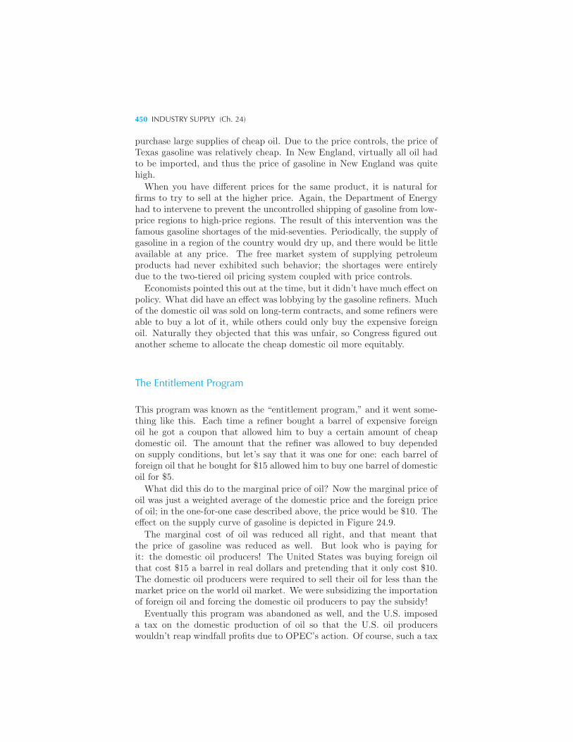
450 INDUSTRY SUPPLY (Ch. 24)
purchase large supplies of cheap oil. Due to the price controls, the price ofTexas gasoline was relatively cheap. In New England, virtually all oil hadto be imported, and thus the price of gasoline in New England was quitehigh.
When you have different prices for the same product, it is natural forfirms to try to sell at the higher price. Again, the Department of Energyhad to intervene to prevent the uncontrolled shipping of gasoline from low-price regions to high-price regions. The result of this intervention was thefamous gasoline shortages of the mid-seventies. Periodically, the supply ofgasoline in a region of the country would dry up, and there would be littleavailable at any price. The free market system of supplying petroleumproducts had never exhibited such behavior; the shortages were entirelydue to the two-tiered oil pricing system coupled with price controls.
Economists pointed this out at the time, but it didn’t have much effect onpolicy. What did have an effect was lobbying by the gasoline refiners. Muchof the domestic oil was sold on long-term contracts, and some refiners wereable to buy a lot of it, while others could only buy the expensive foreignoil. Naturally they objected that this was unfair, so Congress figured outanother scheme to allocate the cheap domestic oil more equitably.
The Entitlement Program
This program was known as the “entitlement program,” and it went some-thing like this. Each time a refiner bought a barrel of expensive foreignoil he got a coupon that allowed him to buy a certain amount of cheapdomestic oil. The amount that the refiner was allowed to buy dependedon supply conditions, but let’s say that it was one for one: each barrel offoreign oil that he bought for $15 allowed him to buy one barrel of domesticoil for $5.
What did this do to the marginal price of oil? Now the marginal price ofoil was just a weighted average of the domestic price and the foreign priceof oil; in the one-for-one case described above, the price would be $10. Theeffect on the supply curve of gasoline is depicted in Figure 24.9.
The marginal cost of oil was reduced all right, and that meant thatthe price of gasoline was reduced as well. But look who is paying forit: the domestic oil producers! The United States was buying foreign oilthat cost $15 a barrel in real dollars and pretending that it only cost $10.The domestic oil producers were required to sell their oil for less than themarket price on the world oil market. We were subsidizing the importationof foreign oil and forcing the domestic oil producers to pay the subsidy!
Eventually this program was abandoned as well, and the U.S. imposeda tax on the domestic production of oil so that the U.S. oil producerswouldn’t reap windfall profits due to OPEC’s action. Of course, such a tax
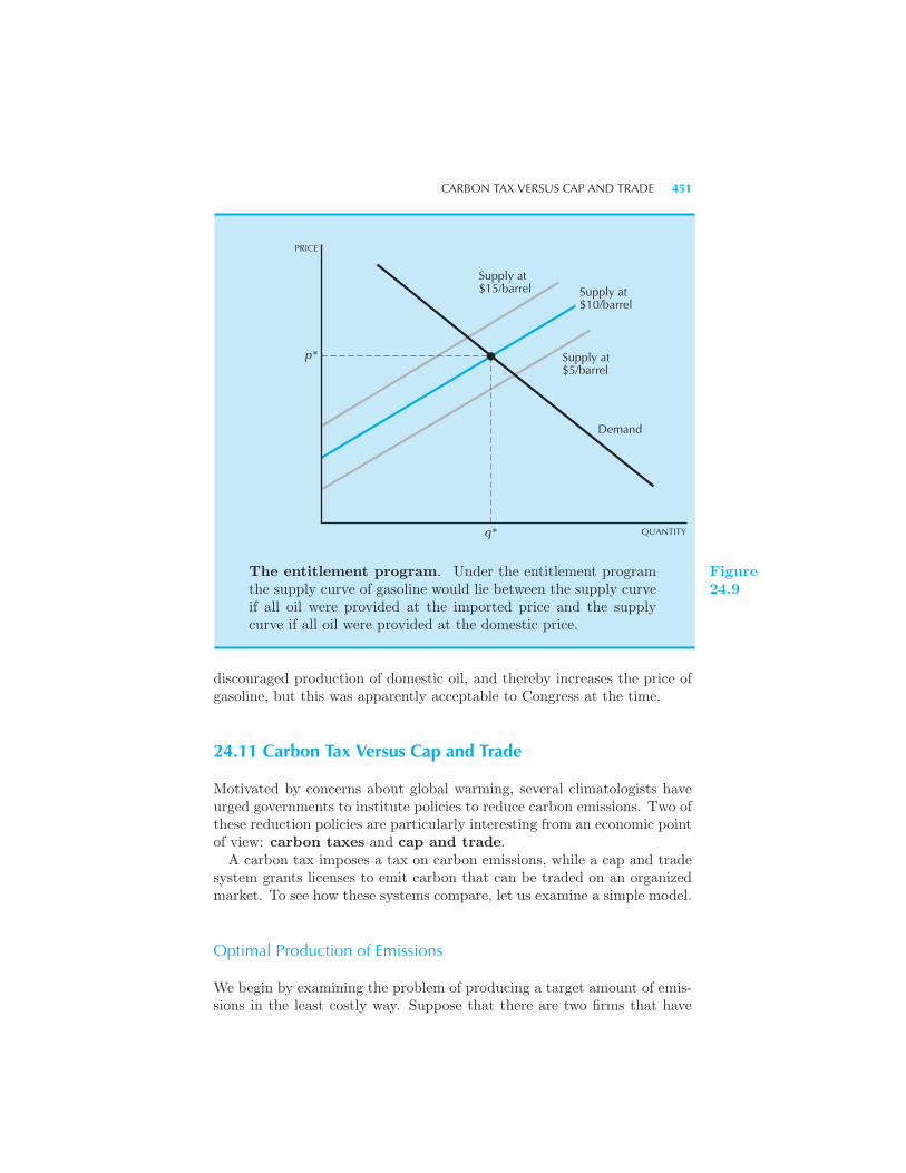
CARBON TAX VERSUS CAP AND TRADE 451
Supply at$10/barrel
Supply at$5/barrel
Supply at$15/barrel
Demand
PRICE
QUANTITYq*
p*
The entitlement program. Under the entitlement programthe supply curve of gasoline would lie between the supply curveif all oil were provided at the imported price and the supplycurve if all oil were provided at the domestic price.
Figure24.9
discouraged production of domestic oil, and thereby increases the price ofgasoline, but this was apparently acceptable to Congress at the time.
24.11 Carbon Tax Versus Cap and Trade
Motivated by concerns about global warming, several climatologists haveurged governments to institute policies to reduce carbon emissions. Two ofthese reduction policies are particularly interesting from an economic pointof view: carbon taxes and cap and trade.
A carbon tax imposes a tax on carbon emissions, while a cap and tradesystem grants licenses to emit carbon that can be traded on an organizedmarket. To see how these systems compare, let us examine a simple model.
Optimal Production of Emissions
We begin by examining the problem of producing a target amount of emis-sions in the least costly way. Suppose that there are two firms that have
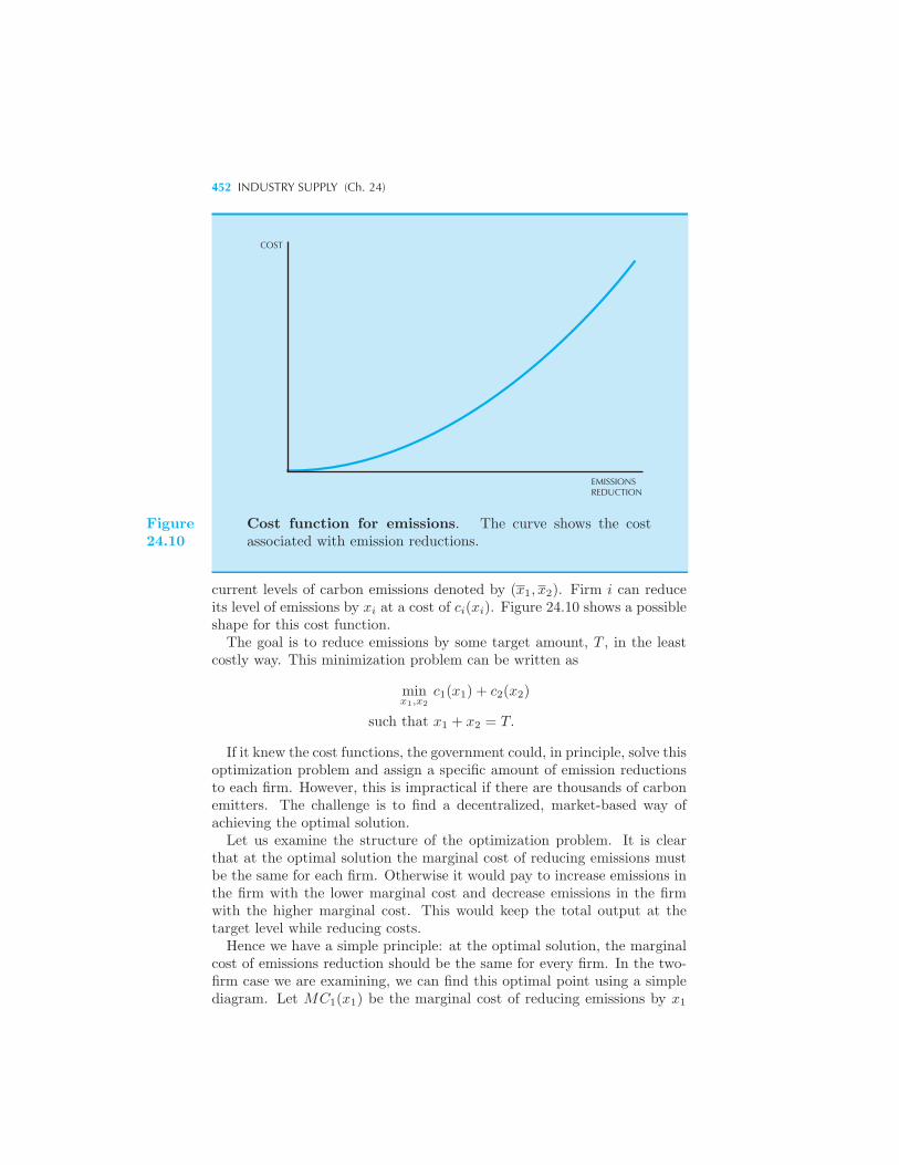
452 INDUSTRY SUPPLY (Ch. 24)
COST
EMISSIONSREDUCTION
Figure24.10
Cost function for emissions. The curve shows the costassociated with emission reductions.
current levels of carbon emissions denoted by (x1, x2). Firm i can reduceits level of emissions by xi at a cost of ci(xi). Figure 24.10 shows a possibleshape for this cost function.The goal is to reduce emissions by some target amount, T , in the least
costly way. This minimization problem can be written as
minx1,x2
c1(x1) + c2(x2)
such that x1 + x2 = T.
If it knew the cost functions, the government could, in principle, solve thisoptimization problem and assign a specific amount of emission reductionsto each firm. However, this is impractical if there are thousands of carbonemitters. The challenge is to find a decentralized, market-based way ofachieving the optimal solution.Let us examine the structure of the optimization problem. It is clear
that at the optimal solution the marginal cost of reducing emissions mustbe the same for each firm. Otherwise it would pay to increase emissions inthe firm with the lower marginal cost and decrease emissions in the firmwith the higher marginal cost. This would keep the total output at thetarget level while reducing costs.Hence we have a simple principle: at the optimal solution, the marginal
cost of emissions reduction should be the same for every firm. In the two-firm case we are examining, we can find this optimal point using a simplediagram. Let MC1(x1) be the marginal cost of reducing emissions by x1
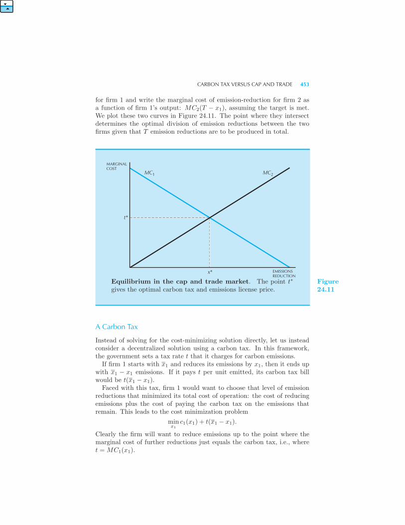
CARBON TAX VERSUS CAP AND TRADE 453
for firm 1 and write the marginal cost of emission-reduction for firm 2 asa function of firm 1’s output: MC2(T − x1), assuming the target is met.We plot these two curves in Figure 24.11. The point where they intersectdetermines the optimal division of emission reductions between the twofirms given that T emission reductions are to be produced in total.
MARGINALCOST
EMISSIONSREDUCTION
t*
x*
MC1 MC2
Equilibrium in the cap and trade market. The point t∗
gives the optimal carbon tax and emissions license price.Figure24.11
A Carbon Tax
Instead of solving for the cost-minimizing solution directly, let us insteadconsider a decentralized solution using a carbon tax. In this framework,the government sets a tax rate t that it charges for carbon emissions.
If firm 1 starts with x1 and reduces its emissions by x1, then it ends upwith x1 − x1 emissions. If it pays t per unit emitted, its carbon tax billwould be t(x1 − x1).Faced with this tax, firm 1 would want to choose that level of emission
reductions that minimized its total cost of operation: the cost of reducingemissions plus the cost of paying the carbon tax on the emissions thatremain. This leads to the cost minimization problem
minx1
c1(x1) + t(x1 − x1).
Clearly the firm will want to reduce emissions up to the point where themarginal cost of further reductions just equals the carbon tax, i.e., wheret = MC1(x1).
454 INDUSTRY SUPPLY (Ch. 24)
If the carbon tax is set to be the rate t∗, as determined in Figure 24.11,then the total amount of carbon emissions will be the targeted amount,T . Thus the carbon tax gives a decentralized way to achieve the optimaloutcome.
Cap and Trade
Suppose, alternatively that there is no carbon tax, but that the governmentissues tradable emissions licenses. Each license allows the firm thatholds it to produce a certain amount of carbon emissions. The governmentchooses the number of emissions licenses to achieve the target reduction.We imagine a market in these licenses so each firm can buy a license
to emit x units of carbon at a price of p per unit. The cost to firm 1 ofreducing its emissions by x1 is c1(x1) + p(x1 − x1). Clearly the firm willwant to operate where the price of an emissions license equals the marginalcost, p = MC1(x1). That is, it will choose the level of emissions at thepoint where the cost of reducing carbon emissions by one unit would justequal the cost saved by not having to purchase a license.Hence the marginal cost curve gives us the supply of emissions as a
function of the price. The equilibrium price is the price where the totalsupply of emissions equals the target amount T . The associated price isthe same as the optimal carbon tax rate t∗ in Figure 24.11.The question that remains is how to distribute the licenses. One way
would be to have the government sell the licenses to firms. This is essen-tially the same as the carbon tax system. The government could pick aprice and sell however many licenses are demanded at that price. Alter-natively, it could pick a target level of emissions and auction off permits,letting the firms themselves determine a price. This is one type of “cap andtrade” system. Both of these policies should lead to essentially the samemarket-clearing price.Another possibility would be for the government to hand out the licenses
to the firms according to some formula. This formula could be based ona variety of criteria, but presumably an important reason to award thesevaluable permits would be building political support for the program. Per-mits might be handed out based on objective criteria, such as which firmshave the most employees, or they might be handed out based on whichfirms have donated the most to some political causes.From the economic point of view, it doesn’t matter whether the gov-
ernment owns the licenses and sells them to the firms (which is basicallya carbon tax system) or whether the firms are given the licenses and sellthem to each other (which is basically cap and trade).If a cap and trade system is created, firms will find it attractive to invest
in ways to acquire the emission permits. For example, they would wantto lobby Congress for such licenses. These lobbying expenditures should

REVIEW QUESTIONS 455
be counted as part of the cost of the system, as described in our earlierdiscussion of rent seeking. Of course, the carbon tax system would also besubject to similar lobbying. Firms would undoubtedly seek special carbontax exemptions for one reason or another, but it has been argued that thecarbon tax system is less susceptible to political manipulation than a capand trade system.
Summary
1. The short-run supply curve of an industry is just the horizontal sum ofthe supply curves of the individual firms in that industry.
2. The long-run supply curve of an industry must take into account theexit and entry of firms in the industry.
3. If there is free entry and exit, then the long-run equilibrium will involvethe maximum number of firms consistent with nonnegative profits. Thismeans that the long-run supply curve will be essentially horizontal at aprice equal to the minimum average cost.
4. If there are forces preventing the entry of firms into a profitable industry,the factors that prevent entry will earn economic rents. The rent earned isdetermined by the price of the output of the industry.
REVIEW QUESTIONS
1. If S1(p) = p−10 and S2(p) = p−15, then at what price does the industrysupply curve have a kink in it?
2. In the short run the demand for cigarettes is totally inelastic. In the longrun, suppose that it is perfectly elastic. What is the impact of a cigarettetax on the price that consumers pay in the short run and in the long run?
3. True or false? Convenience stores near the campus have high pricesbecause they have to pay high rents.
4. True or false? In long-run industry equilibrium no firm will be losingmoney.
5. According to the model presented in this chapter, what determines theamount of entry or exit a given industry experiences?
6. The model of entry presented in this chapter implies that the more firmsin a given industry, the (steeper, flatter) is the long-run industry supplycurve.

456 INDUSTRY SUPPLY (Ch. 24)
7. A New York City cab operator appears to be making positive profits inthe long run after carefully accounting for the operating and labor costs.Does this violate the competitive model? Why or why not?
CHAPTER 25
MONOPOLY
In the preceding chapters we have analyzed the behavior of a competitiveindustry, a market structure that is most likely when there are a largenumber of small firms. In this chapter we turn to the opposite extremeand consider an industry structure when there is only one firm in theindustry—a monopoly.When there is only one firm in a market, that firm is very unlikely to
take the market price as given. Instead, a monopoly would recognize itsinfluence over the market price and choose that level of price and outputthat maximized its overall profits.Of course, it can’t choose price and output independently; for any given
price, the monopoly will be able to sell only what the market will bear. Ifit chooses a high price, it will be able to sell only a small quantity. Thedemand behavior of the consumers will constrain the monopolist’s choiceof price and quantity.We can view the monopolist as choosing the price and letting the con-
sumers choose how much they wish to buy at that price, or we can think ofthe monopolist as choosing the quantity, and letting the consumers decidewhat price they will pay for that quantity. The first approach is probablymore natural, but the second turns out to be analytically more convenient.Of course, both approaches are equivalent when done correctly.
458 MONOPOLY (Ch. 25)
25.1 Maximizing Profits
We begin by studying the monopolist’s profit-maximization problem. Letus use p(y) to denote the market inverse demand curve and c(y) to denotethe cost function. Let r(y) = p(y)y denote the revenue function of themonopolist. The monopolist’s profit-maximization problem then takes theform
maxy
r(y)− c(y).
The optimality condition for this problem is straightforward: at the op-timal choice of output we must have marginal revenue equal to marginalcost. If marginal revenue were less than marginal cost it would pay the firmto decrease output, since the savings in cost would more than make up forthe loss in revenue. If the marginal revenue were greater than the marginalcost, it would pay the firm to increase output. The only point where thefirm has no incentive to change output is where marginal revenue equalsmarginal cost.In terms of algebra, we can write the optimization condition as
MR = MC
orΔr
Δy=
Δc
Δy.
The same MR = MC condition has to hold in the case of a competitivefirm; in that case, marginal revenue is equal to the price and the conditionreduces to price equals marginal cost.In the case of a monopolist, the marginal revenue term is slightly more
complicated. If the monopolist decides to increase its output by Δy, thereare two effects on revenues. First it sells more output and receives a revenueof pΔy from that. But second, the monopolist pushes the price down byΔp and it gets this lower price on all the output it has been selling.Thus the total effect on revenues of changing output by Δy will be
Δr = pΔy + yΔp,
so that the change in revenue divided by the change in output—the mar-ginal revenue—is
Δr
Δy= p+
Δp
Δyy.
(This is exactly the same derivation we went through in our discussion ofmarginal revenue in Chapter 15. You might want to review that materialbefore proceeding.)
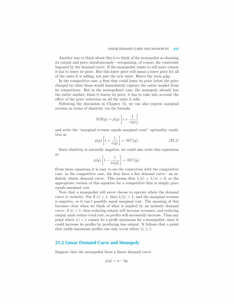
LINEAR DEMAND CURVE AND MONOPOLY 459
Another way to think about this is to think of the monopolist as choosingits output and price simultaneously—recognizing, of course, the constraintimposed by the demand curve. If the monopolist wants to sell more outputit has to lower its price. But this lower price will mean a lower price for allof the units it is selling, not just the new units. Hence the term yΔp.
In the competitive case, a firm that could lower its price below the pricecharged by other firms would immediately capture the entire market fromits competitors. But in the monopolistic case, the monopoly already hasthe entire market; when it lowers its price, it has to take into account theeffect of the price reduction on all the units it sells.Following the discussion in Chapter 15, we can also express marginal
revenue in terms of elasticity via the formula
MR(y) = p(y)
[1 +
1
ε(y)
]
and write the “marginal revenue equals marginal costs” optimality condi-tion as
p(y)
[1 +
1
ε(y)
]= MC(y). (25.1)
Since elasticity is naturally negative, we could also write this expressionas
p(y)
[1− 1
|ε(y)|
]= MC(y).
From these equations it is easy to see the connection with the competitivecase: in the competitive case, the firm faces a flat demand curve—an in-finitely elastic demand curve. This means that 1/|ε| = 1/∞ = 0, so theappropriate version of this equation for a competitive firm is simply priceequals marginal cost.Note that a monopolist will never choose to operate where the demand
curve is inelastic. For if |ε| < 1, then 1/|ε| > 1, and the marginal revenueis negative, so it can’t possibly equal marginal cost. The meaning of thisbecomes clear when we think of what is implied by an inelastic demandcurve: if |ε| < 1, then reducing output will increase revenues, and reducingoutput must reduce total cost, so profits will necessarily increase. Thus anypoint where |ε| < 1 cannot be a profit maximum for a monopolist, since itcould increase its profits by producing less output. It follows that a pointthat yields maximum profits can only occur where |ε| ≥ 1.
25.2 Linear Demand Curve and Monopoly
Suppose that the monopolist faces a linear demand curve
p(y) = a− by.
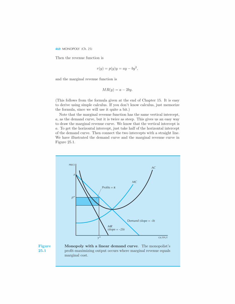
460 MONOPOLY (Ch. 25)
Then the revenue function is
r(y) = p(y)y = ay − by2,
and the marginal revenue function is
MR(y) = a− 2by.
(This follows from the formula given at the end of Chapter 15. It is easyto derive using simple calculus. If you don’t know calculus, just memorizethe formula, since we will use it quite a bit.)
Note that the marginal revenue function has the same vertical intercept,a, as the demand curve, but it is twice as steep. This gives us an easy wayto draw the marginal revenue curve. We know that the vertical intercept isa. To get the horizontal intercept, just take half of the horizontal interceptof the demand curve. Then connect the two intercepts with a straight line.We have illustrated the demand curve and the marginal revenue curve inFigure 25.1.
PRICE
Profits = π
Demand (slope = –b)
MR(slope = –2b)
y* OUTPUT
MC
AC
a
p*
Figure25.1
Monopoly with a linear demand curve. The monopolist’sprofit-maximizing output occurs where marginal revenue equalsmarginal cost.
MARKUP PRICING 461
The optimal output, y∗, is where the marginal revenue curve intersectsthe marginal cost curve. The monopolist will then charge the maximumprice it can get at this output, p(y∗). This gives the monopolist a revenueof p(y∗)y∗ from which we subtract the total cost c(y∗) = AC(y∗)y∗, leavinga profit area as illustrated.
25.3 Markup Pricing
We can use the elasticity formula for the monopolist to express its optimalpricing policy in another way. Rearranging equation (25.1) we have
p(y) =MC(y∗)
1− 1/|ε(y)| . (25.2)
This formulation indicates that the market price is a markup over marginalcost, where the amount of the markup depends on the elasticity of demand.The markup is given by
1
1− 1/|ε(y)| .
Since the monopolist always operates where the demand curve is elastic,we are assured that |ε| > 1, and thus the markup is greater than 1.
In the case of a constant-elasticity demand curve, this formula is espe-cially simple since ε(y) is a constant. A monopolist who faces a constant-elasticity demand curve will charge a price that is a constant markupon marginal cost. This is illustrated in Figure 25.2. The curve labeledMC/(1− 1/|ε|) is a constant fraction higher than the marginal cost curve;the optimal level of output occurs where p = MC/(1− 1/|ε|).
EXAMPLE: The Impact of Taxes on a Monopolist
Let us consider a firm with constant marginal costs and ask what happensto the price charged when a quantity tax is imposed. Clearly the marginalcosts go up by the amount of the tax, but what happens to the marketprice?Let’s first consider the case of a linear demand curve, as depicted in
Figure 25.3. When the marginal cost curve, MC, shifts up by the amountof the tax toMC+t, the intersection of marginal revenue and marginal costmoves to the left. Since the demand curve is half as steep as the marginalrevenue curve, the price goes up by half the amount of the tax.This is easy to see algebraically. The marginal revenue equals marginal
cost plus the tax condition is
a− 2by = c+ t.
462 MONOPOLY (Ch. 25)
PRICE
MC1 – 1/|ε|
MC
Demand
p*
y* OUTPUT
Figure25.2
Monopoly with constant elasticity demand. To locate theprofit-maximizing output level we find the output level wherethe curve MC/(1− 1/|ε|) crosses the demand curve.
Solving for y yields
y =a− c− t
2b.
Thus the change in output is given by
Δy
Δt= − 1
2b.
The demand curve isp(y) = a− by,
so price will change by −b times the change in output:
Δp
Δt= −b×− 1
2b=
1
2.
In this calculation the factor 1/2 occurs because of the assumptions ofthe linear demand curve and constant marginal costs. Together these as-sumptions imply that the price rises by less than the tax increase. Is thislikely to be true in general?The answer is no—in general a tax may increase the price by more or
less than the amount of the tax. For an easy example, consider the case ofa monopolist facing a constant-elasticity demand curve. Then we have
p =c+ t
1− 1/|ε| ,
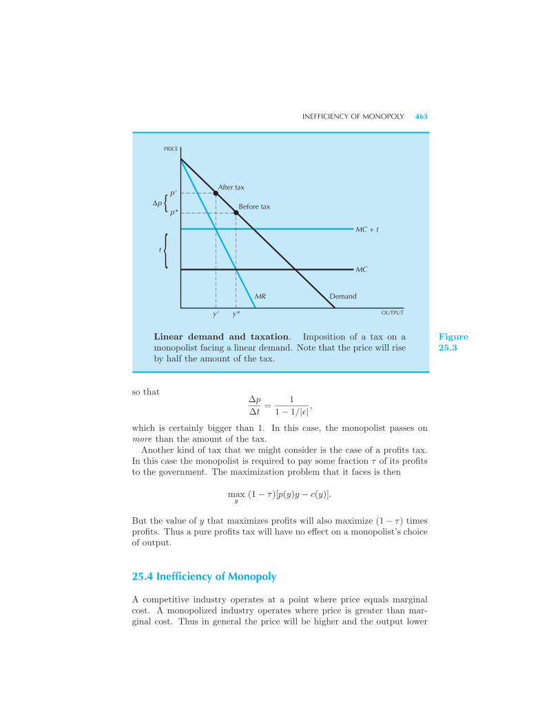
INEFFICIENCY OF MONOPOLY 463
{
{
p'
p*
t
Δp
PRICE
After tax
Before tax
MR Demand
OUTPUT
MC
MC + t
y' y*
Linear demand and taxation. Imposition of a tax on amonopolist facing a linear demand. Note that the price will riseby half the amount of the tax.
Figure25.3
so thatΔp
Δt=
1
1− 1/|ε| ,
which is certainly bigger than 1. In this case, the monopolist passes onmore than the amount of the tax.Another kind of tax that we might consider is the case of a profits tax.
In this case the monopolist is required to pay some fraction τ of its profitsto the government. The maximization problem that it faces is then
maxy
(1− τ)[p(y)y − c(y)].
But the value of y that maximizes profits will also maximize (1− τ) timesprofits. Thus a pure profits tax will have no effect on a monopolist’s choiceof output.
25.4 Inefficiency of Monopoly
A competitive industry operates at a point where price equals marginalcost. A monopolized industry operates where price is greater than mar-ginal cost. Thus in general the price will be higher and the output lower
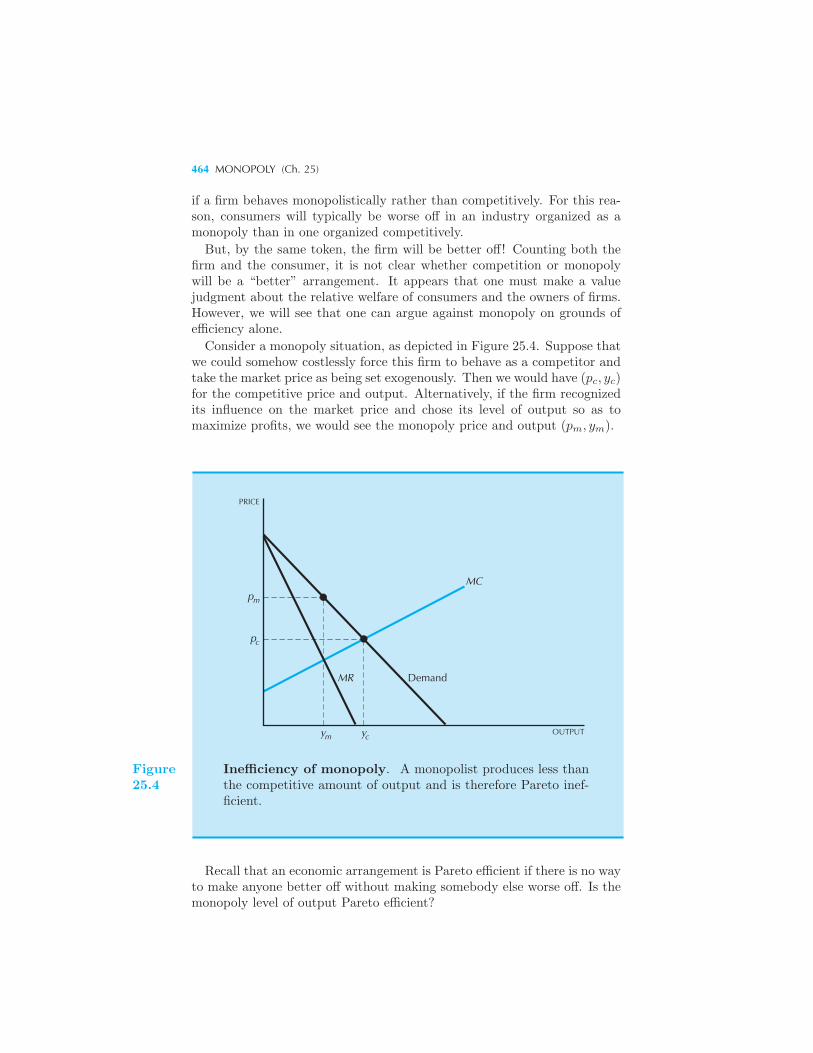
464 MONOPOLY (Ch. 25)
if a firm behaves monopolistically rather than competitively. For this rea-son, consumers will typically be worse off in an industry organized as amonopoly than in one organized competitively.
But, by the same token, the firm will be better off! Counting both thefirm and the consumer, it is not clear whether competition or monopolywill be a “better” arrangement. It appears that one must make a valuejudgment about the relative welfare of consumers and the owners of firms.However, we will see that one can argue against monopoly on grounds ofefficiency alone.
Consider a monopoly situation, as depicted in Figure 25.4. Suppose thatwe could somehow costlessly force this firm to behave as a competitor andtake the market price as being set exogenously. Then we would have (pc, yc)for the competitive price and output. Alternatively, if the firm recognizedits influence on the market price and chose its level of output so as tomaximize profits, we would see the monopoly price and output (pm, ym).
OUTPUTyym c
p
p
m
c
MR Demand
MC
PRICE
Figure25.4
Inefficiency of monopoly. A monopolist produces less thanthe competitive amount of output and is therefore Pareto inef-ficient.
Recall that an economic arrangement is Pareto efficient if there is no wayto make anyone better off without making somebody else worse off. Is themonopoly level of output Pareto efficient?
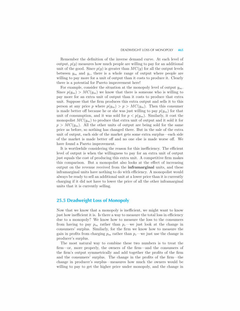
DEADWEIGHT LOSS OF MONOPOLY 465
Remember the definition of the inverse demand curve. At each level ofoutput, p(y) measures how much people are willing to pay for an additionalunit of the good. Since p(y) is greater than MC(y) for all the output levelsbetween ym and yc, there is a whole range of output where people arewilling to pay more for a unit of output than it costs to produce it. Clearlythere is a potential for Pareto improvement here!For example, consider the situation at the monopoly level of output ym.
Since p(ym) > MC(ym) we know that there is someone who is willing topay more for an extra unit of output than it costs to produce that extraunit. Suppose that the firm produces this extra output and sells it to thisperson at any price p where p(ym) > p > MC(ym). Then this consumeris made better off because he or she was just willing to pay p(ym) for thatunit of consumption, and it was sold for p < p(ym). Similarly, it cost themonopolist MC(ym) to produce that extra unit of output and it sold it forp > MC(ym). All the other units of output are being sold for the sameprice as before, so nothing has changed there. But in the sale of the extraunit of output, each side of the market gets some extra surplus—each sideof the market is made better off and no one else is made worse off. Wehave found a Pareto improvement.It is worthwhile considering the reason for this inefficiency. The efficient
level of output is when the willingness to pay for an extra unit of outputjust equals the cost of producing this extra unit. A competitive firm makesthis comparison. But a monopolist also looks at the effect of increasingoutput on the revenue received from the inframarginal units, and theseinframarginal units have nothing to do with efficiency. A monopolist wouldalways be ready to sell an additional unit at a lower price than it is currentlycharging if it did not have to lower the price of all the other inframarginalunits that it is currently selling.
25.5 Deadweight Loss of Monopoly
Now that we know that a monopoly is inefficient, we might want to knowjust how inefficient it is. Is there a way to measure the total loss in efficiencydue to a monopoly? We know how to measure the loss to the consumersfrom having to pay pm rather than pc—we just look at the change inconsumers’ surplus. Similarly, for the firm we know how to measure thegain in profits from charging pm rather than pc—we just use the change inproducer’s surplus.The most natural way to combine these two numbers is to treat the
firm—or, more properly, the owners of the firm—and the consumers ofthe firm’s output symmetrically and add together the profits of the firmand the consumers’ surplus. The change in the profits of the firm—thechange in producer’s surplus—measures how much the owners would bewilling to pay to get the higher price under monopoly, and the change in
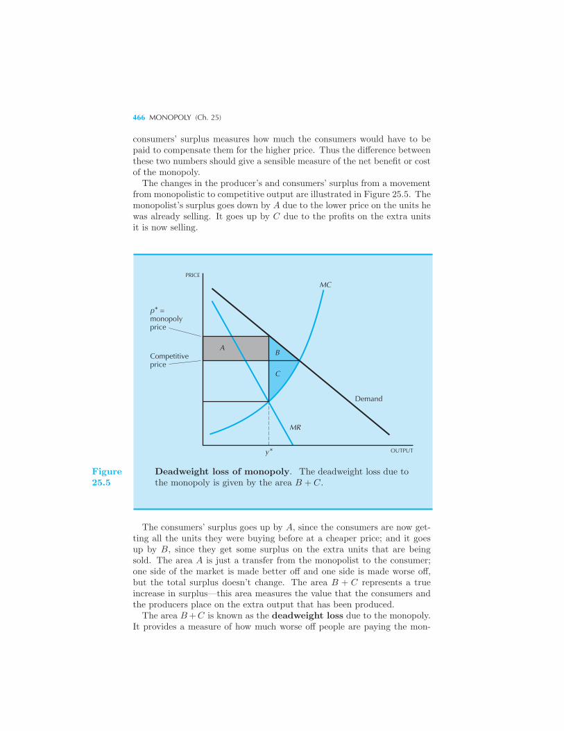
466 MONOPOLY (Ch. 25)
consumers’ surplus measures how much the consumers would have to bepaid to compensate them for the higher price. Thus the difference betweenthese two numbers should give a sensible measure of the net benefit or costof the monopoly.The changes in the producer’s and consumers’ surplus from a movement
from monopolistic to competitive output are illustrated in Figure 25.5. Themonopolist’s surplus goes down by A due to the lower price on the units hewas already selling. It goes up by C due to the profits on the extra unitsit is now selling.
PRICE
OUTPUT
Demand
MR
C
BA
Competitiveprice
p* =monopolyprice
y*
MC
Figure25.5
Deadweight loss of monopoly. The deadweight loss due tothe monopoly is given by the area B + C.
The consumers’ surplus goes up by A, since the consumers are now get-ting all the units they were buying before at a cheaper price; and it goesup by B, since they get some surplus on the extra units that are beingsold. The area A is just a transfer from the monopolist to the consumer;one side of the market is made better off and one side is made worse off,but the total surplus doesn’t change. The area B + C represents a trueincrease in surplus—this area measures the value that the consumers andthe producers place on the extra output that has been produced.The area B+C is known as the deadweight loss due to the monopoly.
It provides a measure of how much worse off people are paying the mon-
DEADWEIGHT LOSS OF MONOPOLY 467
opoly price than paying the competitive price. The deadweight loss due tomonopoly, like the deadweight loss due to a tax, measures the value of thelost output by valuing each unit of lost output at the price that people arewilling to pay for that unit.To see that the deadweight loss measures the value of the lost output,
think about starting at the monopoly point and providing one additinalunit of output. The value of that marginal unit of output is the marketprice. The cost of producing the additional unit of output is the marginalcost. Thus the “social value” of producing an extra unit will be simplythe price minus the marginal cost. Now consider the value of the nextunit of output; again its social value will be the gap between price andmarginal cost at that level of output. And so it goes. As we move fromthe monopoly level of output to the competitive level of output, we “sumup” the distances between the demand curve and the marginal cost curveto generate the value of the lost output due to the monopoly behavior.The total area between the two curves from the monopoly output to thecompetitive output is the deadweight loss.
EXAMPLE: The Optimal Life of a Patent
A patent offers inventors the exclusive right to benefit from their inven-tions for a limited period of time. Thus a patent offers a kind of limitedmonopoly. The reason for offering such patent protection is to encourageinnovation. In the absence of a patent system, it is likely that individualsand firms would be unwilling to invest much in research and development,since any new discoveries that they would make could be copied by com-petitors.In the United States the life of a patent is 17 years. During that period,
the holders of the patent have a monopoly on the invention; after thepatent expires, anyone is free to utilize the technology described in thepatent. The longer the life of a patent, the more gains can be accrued bythe inventors, and thus the more incentive they have to invest in researchand development. However, the longer the monopoly is allowed to exist, themore deadweight loss will be generated. The benefit from a long patent lifeis that it encourages innovation; the cost is that it encourages monopoly.The “optimal” patent life is the period that balances these two conflictingeffects.The problem of determining the optimal patent life has been examined
by William Nordhaus of Yale University.1 As Nordhaus indicates, the prob-lem is very complex and there are many unknown relationships involved.Nevertheless, some simple calculations can give some insight as to whether
1 William Nordhaus, Invention, Growth, and Welfare (Cambridge, Mass.: M.I.T. Press,1969).
468 MONOPOLY (Ch. 25)
the current patent life is wildly out of line with the estimated benefits andcosts described above.
Nordhaus found that for “run-of-the-mill” inventions, a patent life of 17years was roughly 90 percent efficient—meaning that it achieved 90 percentof the maximum possible consumers’ surplus. On the basis of these figures,it does not seem like there is a compelling reason to make drastic changesin the patent system.
EXAMPLE: Patent Thickets
The intellectual property protection offered by patents provides incentivesto innovate, but this right can be abused. Some observers have arguedthat the extensions of intellectual property rights to business processes,software, and other domains has resulted in lower patent quality.
One might think of patents as having three dimensions: length, width,and height. The “length” is the time that the patent protection applies.The “width” is how broadly the claims in the patent are interpreted. The“height” is the standard of novelty applied in determining whether thepatent really represents a new idea. Unfortunately, only the length is easilyquantified. The other aspects of patent quality, breadth, and novelty, canbe quite subjective.
Since it has become so easy to acquire patents in recent years, many firmshave invested in acquiring patent portfolios on nearly every aspect of theirbusiness. Any company that wants to enter a business and compete with anincumbent who owns a broad range of patents may find itself encumberedin a patent thicket.
Even firms that are already well established find it important to investin acquiring a patent portfolio. In 2004, Microsoft paid $440 million toInterTrust Technology to license a portfolio of patents related to computersecurity, and signed a 10-year pact with Sun Microsystems in which itpaid $900 million to resolve patent issues. During 2003–04, Microsoft wasgranted over 1,000 patents.
Why the emphasis on patent portfolios? For large companies like Mi-crosoft, their primary value is to be used as bargaining chips in cross-licenseagreements.
The patent thickets that each company sets up operate like the nuclearmissiles held by the U.S. and USSR during the Cold War. Each had enoughmissiles pointed at the other to create “mutually assured destruction” inthe case that one side attacked. Hence, neither side could risk an attack.
It’s the same issue with patent thickets. If IBM tries to sue HP forpatent infringement, HP would pull out a collection of its own patents andcountersue IBM for infringement in some other technology. Even companiesthat don’t particularly want to patent aspects of their business are forced
NATURAL MONOPOLY 469
to do so in order to acquire the ammunition necessary for defense againstother suits.The “nuclear bomb” option in patent thickets is a “preliminary injunc-
tion.” In certain circumstances, a judge might compel a company to stopselling an item that may be infringing on someone else’s patent. This canbe exceedingly costly. In 1986, Kodak had to completely shut down its in-stant photography business due to a court-ordered injunction. EventuallyKodak had to pay a billion-dollar judgment for patent infringement.An injunction to stop production can be a huge threat, but it has no force
against companies that don’t produce anything. InterTrust, for example,didn’t sell any products—all of its income came from licensing patents.Hence, it could threaten to sue other companies for patent infringementwithout much worry about the threat of countersuits.
EXAMPLE: Managing the Supply of Potatoes
Everyone is familiar with the Organization of Petroleum Exporting Coun-tries (OPEC), the international oil cartel that attempts to influence theprice of oil by setting production quota. Normally, coordinating produc-tion to push up prices is illegal in the United States, but there are someindustries that are exempt from antitrust rules.A notable example is agricultural producers. The 1922 Capper-Volstead
Act specifically exempts farmers from federal antitrust rules. The resulthas been the creation of a number of “agricultural marketing boards” thatattempt to voluntarily regulate the supply of agricultural products.For example, the United Potato Growers of America, formed in March
2005, has signed up potato farmers that represent over 60% of the potatoacreage in the United States. In 2005 it claimed to reduce production ofpotatoes by 6.8 million sacks of potatoes, each weighing about 100 poundsa piece. According to the Wall Street Journal this is equivalent to about1.3 billion orders of french fries.2
25.6 Natural Monopoly
We have seen earlier that the Pareto efficient amount of output in an indus-try occurs where price equals marginal cost. A monopolist produces wheremarginal revenue equals marginal cost and thus produces too little output.It would seem that regulating a monopoly to eliminate the inefficiency ispretty easy—all the regulator has to do is to set price equal to marginal
2 Timothy W. Martin, “This Spud’s Not for You,” Wall Street Journal, September 26,2009.
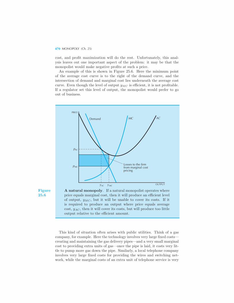
470 MONOPOLY (Ch. 25)
cost, and profit maximization will do the rest. Unfortunately, this anal-ysis leaves out one important aspect of the problem: it may be that themonopolist would make negative profits at such a price.An example of this is shown in Figure 25.6. Here the minimum point
of the average cost curve is to the right of the demand curve, and theintersection of demand and marginal cost lies underneath the average costcurve. Even though the level of output yMC is efficient, it is not profitable.If a regulator set this level of output, the monopolist would prefer to goout of business.
Demand MC AC
PRICE
pAC
pMC
yAC MCy OUTPUT
Losses to the firmfrom marginal costpricing
Figure25.6
A natural monopoly. If a natural monopolist operates whereprice equals marginal cost, then it will produce an efficient levelof output, yMC , but it will be unable to cover its costs. If itis required to produce an output where price equals averagecost, yAC , then it will cover its costs, but will produce too littleoutput relative to the efficient amount.
This kind of situation often arises with public utilities. Think of a gascompany, for example. Here the technology involves very large fixed costs—creating and maintaining the gas delivery pipes—and a very small marginalcost to providing extra units of gas—once the pipe is laid, it costs very lit-tle to pump more gas down the pipe. Similarly, a local telephone companyinvolves very large fixed costs for providing the wires and switching net-work, while the marginal costs of an extra unit of telephone service is very
NATURAL MONOPOLY 471
low. When there are large fixed costs and small marginal costs, you caneasily get the kind of situation described in Figure 25.6. Such a situationis referred to as a natural monopoly.If allowing a natural monopolist to set the monopoly price is undesir-
able due to the Pareto inefficiency, and forcing the natural monopoly toproduce at the competitive price is infeasible due to negative profits, whatis left? For the most part natural monopolies are regulated or operatedby governments. Different countries have adopted different approaches. Insome countries the telephone service is provided by the government and inothers it is provided by private firms that are regulated by the government.Both of these approaches have their advantages and disadvantages.For example, let us consider the case of government regulation of a nat-
ural monopoly. If the regulated firm is to require no subsidy, it must makenonnegative profits, which means it must operate on or above the averagecost curve. If it is to provide service to all who are willing to pay for it,it must also operate on the demand curve. Thus the natural operatingposition for a regulated firm is a point like (pAC , yAC) in Figure 25.6. Herethe firm is selling its product at the average cost of production, so it coversits costs, but it is producing too little output relative to the efficient levelof output.This solution is often adopted as a reasonable pricing policy for a natural
monopolist. Government regulators set the prices that the public utilityis allowed to charge. Ideally these prices are supposed to be prices thatjust allow the firm to break even—produce at a point where price equalsaverage costs.The problem facing the regulators is to determine just what the true
costs of the firm are. Usually there is a public utility commission thatinvestigates the costs of the monopoly in an attempt to determine the trueaverage cost and then sets a price that will cover costs. (Of course, one ofthese costs is the payment that the firm has to make to its shareholdersand other creditors in exchange for the money they have loaned to thefirm.)In the United States these regulatory boards operate at the state and
local level. Typically electricity, natural gas, and telephone service operatein this way. Other natural monopolies like cable TV are usually regulatedat the local level.The other solution to the problem of natural monopoly is to let the gov-
ernment operate it. The ideal solution here in this case is to operate theservice at price equals marginal cost and provide a lump-sum subsidy tokeep the firm in operation. This is often the practice for local public trans-portation systems such as buses and subways. The lump-sum subsidiesmay not reflect inefficient operation per se but rather, simply reflect thelarge fixed costs associated with such public utilities.Then again, the subsidies may just represent inefficiency! The problem
with government-run monopolies is that it is almost as difficult to mea-
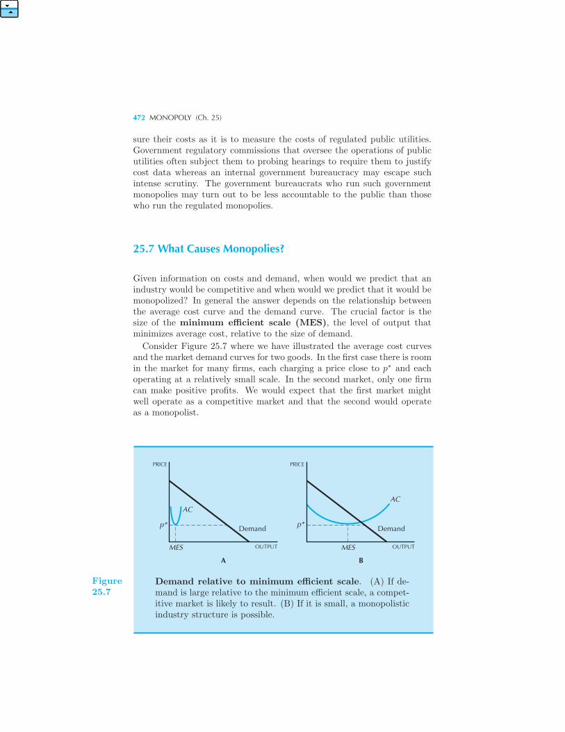
472 MONOPOLY (Ch. 25)
sure their costs as it is to measure the costs of regulated public utilities.Government regulatory commissions that oversee the operations of publicutilities often subject them to probing hearings to require them to justifycost data whereas an internal government bureaucracy may escape suchintense scrutiny. The government bureaucrats who run such governmentmonopolies may turn out to be less accountable to the public than thosewho run the regulated monopolies.
25.7 What Causes Monopolies?
Given information on costs and demand, when would we predict that anindustry would be competitive and when would we predict that it would bemonopolized? In general the answer depends on the relationship betweenthe average cost curve and the demand curve. The crucial factor is thesize of the minimum efficient scale (MES), the level of output thatminimizes average cost, relative to the size of demand.
Consider Figure 25.7 where we have illustrated the average cost curvesand the market demand curves for two goods. In the first case there is roomin the market for many firms, each charging a price close to p∗ and eachoperating at a relatively small scale. In the second market, only one firmcan make positive profits. We would expect that the first market mightwell operate as a competitive market and that the second would operateas a monopolist.
OUTPUT OUTPUTMESMES
Demand Demand
ACAC
PRICE PRICE
A B
p*p*
Figure25.7
Demand relative to minimum efficient scale. (A) If de-mand is large relative to the minimum efficient scale, a compet-itive market is likely to result. (B) If it is small, a monopolisticindustry structure is possible.
WHAT CAUSES MONOPOLIES? 473
Thus the shape of the average cost curve, which in turn is determined bythe underlying technology, is one important aspect that determines whethera market will operate competitively or monopolistically. If the minimumefficient scale of production—the level of output that minimizes averagecosts—is small relative to the size of the market, we might expect thatcompetitive conditions will prevail.
Note that this is a relative statement: what matters is the scale relative tothe market size. We can’t do too much about the minimum efficient scale—that is determined by the technology. But economic policy can influencethe size of the market. If a country chooses nonrestrictive foreign-tradepolicies, so that domestic firms face foreign competition, then the domesticfirms’ ability to influence prices will be much less. Conversely, if a countryadopts restrictive trade policies, so that the size of the market is limitedonly to that country, then monopolistic practices are more likely to takehold.
If monopolies arise because the minimum efficient scale is large relativeto the size of the market, and it is infeasible to increase the size of themarket, then the industry is a candidate for regulation or other sorts ofgovernment intervention. Of course such regulation and intervention arecostly too. Regulatory boards cost money, and the efforts of the firmto satisfy the regulatory boards can be quite expensive. From society’spoint of view, the question should be whether the deadweight loss of themonopoly exceeds the costs of regulation.
A second reason why monopoly might occur is that several different firmsin an industry might be able to collude and restrict output in order to raiseprices and thereby increase their profits. When firms collude in this wayand attempt to reduce output and increase price, we say the industry isorganized as a cartel.
Cartels are illegal. The Antitrust Division of the Justice Department andthe Bureau of Competition of the Federal Trade Commission are chargedwith searching for evidence of noncompetitive behavior on the part of firms.If the government can establish that a group of firms attempted to restrictoutput or engaged in certain other anticompetitive practices, the firms inquestion can be forced to pay heavy fines.
On the other hand, an industry may have one dominant firm purelyby historical accident. If one firm is first to enter some market, it mayhave enough of a cost advantage to be able to discourage other firms fromentering the industry. Suppose, for example, that there are very large“tooling-up” costs to entering an industry. Then the incumbent—the firmalready in the industry—may under certain conditions be able to convincepotential entrants that it will cut its prices drastically if they attemptto enter the industry. By preventing entry in this manner, a firm caneventually dominate a market. We will study an example of pricing toprevent entry in Chapter 29.
474 MONOPOLY (Ch. 25)
EXAMPLE: Diamonds Are Forever
The De Beers diamond cartel was formed by Sir Ernest Oppenheimer, aSouth African mine operator, in 1930. It has since grown into one of theworld’s most successful cartels. De Beers handles over 80% of the world’syearly production of diamonds and has managed to maintain this near-monopoly for several decades. Over the years, De Beers has developedseveral mechanism to maintain control of the diamond market.First, it maintains considerable stocks of diamonds of all types. If a
producer attempts to sell outside the cartel, De Beers can quickly flood themarket with the same type of diamond, thereby punishing the defector fromthe cartel. Second, large producers’ quotas are based on the proportionof total sales. When the market is weak, everyone’s production quotais reduced proportionally, thereby automatically increasing scarcity andraising prices.Third, De Beers is involved at both the mining and wholesaling levels of
diamond production. In the wholesale market diamonds are sold to cuttersin boxes of assorted diamonds: buyers take a whole box or nothing—theycannot choose individual stones. If the market is weak for a certain sizeof diamond, De Beers can reduce the number of those diamonds offered inthe boxes, thereby making them more scarce.Finally, De Beers can influence the direction of final demand for diamonds
by the $110 million a year it spends on advertising. Again, this advertisingcan be adjusted to encourage demand for the types and sizes of diamondsthat are in relatively scarce supply.3
EXAMPLE: Pooling in Auction Markets
Adam Smith once said “People of the same trade seldom meet together,even for merriment and diversion, but the conversation ends in a conspir-acy against the public, or in some contrivance to raise prices.” Biddingpools in auctions provide an illustrative example of Smith’s observation.In 1988 the Justice Department charged 12 Philadelphia antique dealerswith antitrust violations for their participation in this particular kind of“conspiracy against the public.”4
3 A short description of the diamond market can be found in “The cartel lives toface another threat,” The Economist, January 10, 1987, 58–60. A more detaileddescription can be found in Edward J. Epstein, Cartel (New York: Putnam, 1978).
4 See Meg Cox, “At Many Auctions, Illegal Bidding Thrives As a Longtime PracticeAmong Dealers,” Wall Street Journal, February 19, 1988, which served as the sourcefor this example.
WHAT CAUSES MONOPOLIES? 475
The dealers were accused of participating in “bidding rings,” or “pools,”at antique furniture auctions. The members of a pool would appoint onemember to bid on certain items. If this bidder succeeded in acquiringan item, the participating dealers would then hold a subsequent privateauction, called a “knockout,” in which the members of the pool bid amongthemselves for the item. This practice allowed the members of the pool toacquire the items at much lower prices than would have prevailed if theyhad bid separately; in many cases the prices in the knockout auctions were50 to 100 percent greater than the prices paid to the original sellers of thegoods.
The dealers were surprised by the Justice Department suit; they consid-ered pooling a common business practice in their trade and did not think itwas illegal. They thought of the pools as a tradition of cooperation amongthemselves; being invited to join a pool was considered a “mark of dis-tinction.” According to one dealer, “The day I was allowed to go into thepool was a banner day. If you weren’t in the pool, you weren’t consideredmuch of a dealer.” The dealers were so naive that they kept careful recordsof their payments in the knockout auctions, which were later used by theJustice Department in the suits against the dealers.
The Justice Department argued “if they are joining together to hold downthe price [received by the seller] that is illegal.” The Justice Departmentview prevailed over that of the dealers: 11 of the 12 dealers pleaded guiltyand settled the matter with fines of $1,000 to $50,000 and probation. Thedealer who held out for a jury trial was found guilty and sentenced to 30days of house arrest and a fine of $30,000.
EXAMPLE: Price Fixing in Computer Memory Markets
DRAM chips are the “dynamic random access memory” chips that go inyour computer. They are pretty much an undifferentiated commodity prod-uct and the market for DRAMs is (usually) highly competitive. However,there are allegations that several DRAM producers conspired to fix pricesand charge computer makers a higher price than would have obtained underpurely competitive conditions. Apple Computer, Compaq, Dell, Gateway,HP, and IBM were apparently affected by this conspiracy.
The Department of Justice started investigating these allegations in 2002.In September 2004, Infineon, a German DRAM manufacturer, pleadedguilty to charges of price fixing, and agreed to pay a $160 million fine.This was the third largest criminal fine ever imposed by the Departmentof Justice’s antitrust division.
According to the court documents, Infineon was charged with “Partic-ipating in meetings, conversations, and communications with competitorsto discuss the prices of DRAM to be sold to certain customers; Agreeing to
476 MONOPOLY (Ch. 25)
price levels of DRAM to be sold to certain customers; Exchanging informa-tion on sales of DRAM to certain customers, for the purpose of monitoringand enforcing the agreed-upon prices.”Subsequently, four executives at Infineon were sentenced to prison terms
and had to pay hefty fines. The antitrust authorities take price fixing veryseriously, and the consequences to companies and individuals that engagein such activities can be severe.
Summary
1. When there is only a single firm in an industry, we say that it is amonopoly.
2. A monopolist operates at a point where marginal revenue equals mar-ginal cost. Hence a monopolist charges a price that is a markup on marginalcost, where the size of the markup depends on the elasticity of demand.
3. Since a monopolist charges a price in excess of marginal cost, it willproduce an inefficient amount of output. The size of the inefficiency canbe measured by the deadweight loss—the net loss of consumers’ and theproducer’s surplus.
4. A natural monopoly occurs when a firm cannot operate at an efficientlevel of output without losing money. Many public utilities are naturalmonopolies of this sort and are therefore regulated by the government.
5. Whether an industry is competitive or monopolized depends in part onthe nature of technology. If the minimum efficient scale is large relative todemand, then the market is likely to be monopolized. But if the minimumefficient scale is small relative to demand, there is room for many firms inthe industry, and there is a hope for a competitive market structure.
REVIEW QUESTIONS
1. The market demand curve for heroin is said to be highly inelastic. Heroinsupply is also said to be monopolized by the Mafia, which we assume to beinterested in maximizing profits. Are these two statements consistent?
2. The monopolist faces a demand curve given by D(p) = 100−2p. Its costfunction is c(y) = 2y. What is its optimal level of output and price?
3. The monopolist faces a demand curve given by D(p) = 10p−3. Its costfunction is c(y) = 2y. What is its optimal level of output and price?
APPENDIX 477
4. If D(p) = 100/p and c(y) = y2, what is the optimal level of output ofthe monopolist? (Be careful.)
5. A monopolist with constant marginal cost is producing where |ε| = 3.The government imposes a quantity tax of $6 per unit of output. If thedemand curve facing the monopolist is linear, how much does the pricerise?
6. What is the answer to the above question if the demand curve facing themonopolist has constant elasticity?
7. If the demand curve facing the monopolist has a constant elasticity of 2,then what will be the monopolist’s markup on marginal cost?
8. The government is considering subsidizing the marginal costs of themonopolist described in the question above. What level of subsidy shouldthe government choose if it wants the monopolist to produce the sociallyoptimal amount of output?
9. Show mathematically that a monopolist always sets its price above mar-ginal cost.
10. True or false? Imposing a quantity tax on a monopolist will alwayscause the market price to increase by the amount of the tax.
11. What problems face a regulatory agency attempting to force a monop-olist to charge the perfectly competitive price?
12. What kinds of economic and technological conditions are conducive tothe formation of monopolies?
APPENDIX
Define the revenue function by r(y) = p(y)y. Then the monopolist’s profit-maximization problem is
max r(y)− c(y).
The first-order condition for this problem is simply
r′(y)− c′(y) = 0,
which implies that marginal revenue should equal marginal cost at the optimalchoice of output.
Differentiating the definition of the revenue function gives r′(y) = p(y)+p′(y)y,and substituting this into the monopolist’s first-order condition yields the alter-native form
p(y) + p′(y)y = c′(y).
478 MONOPOLY (Ch. 25)
The second-order condition for the monopolist’s profit-maximization problemis
r′′(y)− c′′(y) ≤ 0.
This implies thatc′′(y) ≥ r′′(y)
or that the slope of the marginal cost curve exceeds the slope of the marginalrevenue curve.
CHAPTER 26
MONOPOLYBEHAVIOR
In a competitive market there are typically several firms selling an identicalproduct. Any attempt by one of the firms to sell its product at more thanthe market price leads consumers to desert the high-priced firm in favor ofits competitors. In a monopolized market there is only one firm selling agiven product. When a monopolist raises its price it loses some, but notall, of its customers.In reality most industries are somewhere in between these two extremes.
If a gas station in a small town raises the price at which it sells gasolineand it loses most of its customers, it is reasonable to think that this firmmust behave as a competitive firm. If a restaurant in the same town raisesits price and loses only a few of its customers, then it is reasonable to thinkthat this restaurant has some degree of monopoly power.If a firm has some degree of monopoly power it has more options open
to it than a firm in a perfectly competitive industry. For example, it canuse more complicated pricing and marketing strategies than a firm in acompetitive industry. Or it can try to differentiate its product from theproducts sold by its competitors to enhance its market power even further.In this chapter we will examine how firms can enhance and exploit theirmarket power.
480 MONOPOLY BEHAVIOR (Ch. 26)
26.1 Price Discrimination
We have argued earlier that a monopoly operates at an inefficient level ofoutput since it restricts output to a point where people are willing to paymore for extra output than it costs to produce it. The monopolist doesn’twant to produce this extra output, because it would force down the pricethat it would be able to get for all of its output.
But if the monopolist could sell different units of output at differentprices, then we have another story. Selling different units of output atdifferent prices is called price discrimination. Economists generally con-sider the following three kinds of price discrimination:First-degree price discrimination means that the monopolist sells
different units of output for different prices and these prices may differfrom person to person. This is sometimes known as the case of perfectprice discrimination.Second-degree price discrimination means that the monopolist sells
different units of output for different prices, but every individual who buysthe same amount of the good pays the same price. Thus prices differ acrossthe units of the good, but not across people. The most common exampleof this is bulk discounts.Third-degree price discrimination occurs when the monopolist sells
output to different people for different prices, but every unit of output soldto a given person sells for the same price. This is the most common formof price discrimination, and examples include senior citizens’ discounts,student discounts, and so on.Let us look at each of these to see what economics can say about how
price discrimination works.
26.2 First-Degree Price Discrimination
Under first-degree price discrimination, or perfect price discrimi-nation, each unit of the good is sold to the individual who values it mosthighly, at the maximum price that this individual is willing to pay for it.Consider Figure 26.1, which illustrates two consumers’ demand curves
for a good. Think of a reservation price model for demand where the indi-viduals choose integer amounts of the goods and each step in the demandcurve represents a change in the willingness to pay for additional units ofthe good. We have also illustrated (constant) marginal cost curves for thegood.A producer who is able to perfectly price discriminate will sell each unit
of the good at the highest price it will command, that is, at each consumer’sreservation price. Since each unit is sold to each consumer at his or herreservation price for that unit, there is no consumers’ surplus generated in
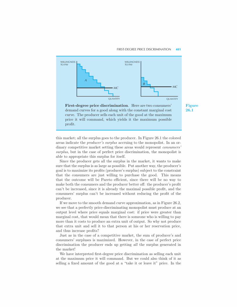
FIRST-DEGREE PRICE DISCRIMINATION 481
WILLINGNESSTO PAY
QUANTITY
MC
A
WILLINGNESSTO PAY
QUANTITY
MCB
First-degree price discrimination. Here are two consumers’demand curves for a good along with the constant marginal costcurve. The producer sells each unit of the good at the maximumprice it will command, which yields it the maximum possibleprofit.
Figure26.1
this market; all the surplus goes to the producer. In Figure 26.1 the coloredareas indicate the producer’s surplus accruing to the monopolist. In an or-dinary competitive market setting these areas would represent consumers’surplus, but in the case of perfect price discrimination, the monopolist isable to appropriate this surplus for itself.Since the producer gets all the surplus in the market, it wants to make
sure that the surplus is as large as possible. Put another way, the producer’sgoal is to maximize its profits (producer’s surplus) subject to the constraintthat the consumers are just willing to purchase the good. This meansthat the outcome will be Pareto efficient, since there will be no way tomake both the consumers and the producer better off: the producer’s profitcan’t be increased, since it is already the maximal possible profit, and theconsumers’ surplus can’t be increased without reducing the profit of theproducer.If we move to the smooth demand curve approximation, as in Figure 26.2,
we see that a perfectly price-discriminating monopolist must produce at anoutput level where price equals marginal cost: if price were greater thanmarginal cost, that would mean that there is someone who is willing to paymore than it costs to produce an extra unit of output. So why not producethat extra unit and sell it to that person at his or her reservation price,and thus increase profits?Just as in the case of a competitive market, the sum of producer’s and
consumers’ surpluses is maximized. However, in the case of perfect pricediscrimination the producer ends up getting all the surplus generated inthe market!We have interpreted first-degree price discrimination as selling each unit
at the maximum price it will command. But we could also think of it asselling a fixed amount of the good at a “take it or leave it” price. In the
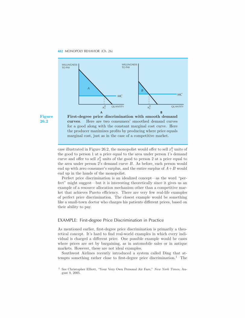
482 MONOPOLY BEHAVIOR (Ch. 26)
A
WILLINGNESSTO PAY
MC
A
QUANTITYx10
B
WILLINGNESSTO PAY
MC
B
QUANTITYx20
Figure26.2
First-degree price discrimination with smooth demandcurves. Here are two consumers’ smoothed demand curvesfor a good along with the constant marginal cost curve. Herethe producer maximizes profits by producing where price equalsmarginal cost, just as in the case of a competitive market.
case illustrated in Figure 26.2, the monopolist would offer to sell x01 units of
the good to person 1 at a price equal to the area under person 1’s demandcurve and offer to sell x0
2 units of the good to person 2 at a price equal tothe area under person 2’s demand curve B. As before, each person wouldend up with zero consumer’s surplus, and the entire surplus of A+B wouldend up in the hands of the monopolist.Perfect price discrimination is an idealized concept—as the word “per-
fect” might suggest—but it is interesting theoretically since it gives us anexample of a resource allocation mechanism other than a competitive mar-ket that achieves Pareto efficiency. There are very few real-life examplesof perfect price discrimination. The closest example would be somethinglike a small-town doctor who charges his patients different prices, based ontheir ability to pay.
EXAMPLE: First-degree Price Discrimination in Practice
As mentioned earlier, first-degree price discrimination is primarily a theo-retical concept. It’s hard to find real-world examples in which every indi-vidual is charged a different price. One possible example would be caseswhere prices are set by bargaining, as in automobile sales or in antiquemarkets. However, these are not ideal examples.Southwest Airlines recently introduced a system called Ding that at-
tempts something rather close to first-degree price discrimination.1 The
1 See Christopher Elliott, “Your Very Own Personal Air Fare,” New York Times, Au-gust 9, 2005.
SECOND-DEGREE PRICE DISCRIMINATION 483
system uses the Internet in a clever way. The user installs a program onher computer and the airline sends special fare offers to the user period-ically. The fares are announced with a “ding” sound, hence the systemname. According to one analyst, the fares offered by Ding were about 30percent lower than comparable fares.
But will these low fares persist? One might also use such a systemto offer higher fares. However, that possibility seems unlikely given theintensely competitive nature of the airline industry. It’s easy to switchback to standard ways of buying tickets if prices start creeping up.
26.3 Second-Degree Price Discrimination
Second-degree price discrimination is also known as the case of non-linear pricing, since it means that the price per unit of output is notconstant but depends on how much you buy. This form of price discrimi-nation is commonly used by public utilities; for example, the price per unitof electricity often depends on how much is bought. In other industriesbulk discounts for large purchases are sometimes available.
Let us consider the case depicted earlier in Figure 26.2. We saw that themonopolist would like to sell an amount x0
1 to person 1 at price A+ costand an amount x0
2 to person 2 at price B+ cost. To set the right prices,the monopolist has to know the demand curves of the consumers; that is,the monopolist has to know the exact willingness to pay of each person.Even if the monopolist knows something about the statistical distributionof willingness to pay—for example, that college students are willing to payless than yuppies for movie tickets—it might be hard to tell a yuppie froma college student when they are standing in line at the ticket booth.
Similarly, an airline ticket agent may know that business travelers arewilling to pay more than tourists for their airplane tickets, but it is oftendifficult to tell whether a particular person is a business traveler or a tourist.If switching from a grey flannel suit to Bermuda shorts would save $500 ontravel expenses, corporate dress codes could change quickly!
The problem with the first-degree price discrimination example depictedin Figure 26.2 is that person 1—the high-willingess-to-pay person—canpretend to be person 2, the low-willingess-to-pay person. The seller mayhave no effective way to tell them apart.
One way to get around this problem is to offer two different price-quantitypackages in the market. One package will be targeted toward the high-demand person, the other package toward the low-demand person. It canoften happen that the monopolist can construct price-quantity packagesthat will induce the consumers to choose the package meant for them; ineconomics jargon, the monopolist constructs price-quantity packages thatgive the consumers an incentive to self select.
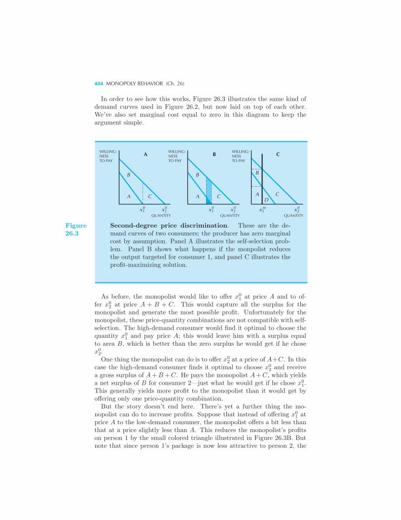
484 MONOPOLY BEHAVIOR (Ch. 26)
In order to see how this works, Figure 26.3 illustrates the same kind ofdemand curves used in Figure 26.2, but now laid on top of each other.We’ve also set marginal cost equal to zero in this diagram to keep theargument simple.
A C
B
AWILLING-NESSTO PAY
QUANTITYx1
0 x20
A C
B
CWILLING-NESSTO PAY
QUANTITYx1
m x20
A C
B
BWILLING-NESSTO PAY
QUANTITYx1
0 x20
D
Figure26.3
Second-degree price discrimination. These are the de-mand curves of two consumers; the producer has zero marginalcost by assumption. Panel A illustrates the self-selection prob-lem. Panel B shows what happens if the monpolist reducesthe output targeted for consumer 1, and panel C illustrates theprofit-maximizing solution.
As before, the monopolist would like to offer x01 at price A and to of-
fer x02 at price A + B + C. This would capture all the surplus for the
monopolist and generate the most possible profit. Unfortunately for themonopolist, these price-quantity combinations are not compatible with self-selection. The high-demand consumer would find it optimal to choose thequantity x0
1 and pay price A; this would leave him with a surplus equalto area B, which is better than the zero surplus he would get if he chosex02.One thing the monopolist can do is to offer x0
2 at a price of A+C. In thiscase the high-demand consumer finds it optimal to choose x0
2 and receivea gross surplus of A+B+C. He pays the monopolist A+C, which yieldsa net surplus of B for consumer 2—just what he would get if he chose x0
1.This generally yields more profit to the monopolist than it would get byoffering only one price-quantity combination.But the story doesn’t end here. There’s yet a further thing the mo-
nopolist can do to increase profits. Suppose that instead of offering x01 at
price A to the low-demand consumer, the monopolist offers a bit less thanthat at a price slightly less than A. This reduces the monopolist’s profitson person 1 by the small colored triangle illustrated in Figure 26.3B. Butnote that since person 1’s package is now less attractive to person 2, the
SECOND-DEGREE PRICE DISCRIMINATION 485
monopolist can now charge more to person 2 for x02! By reducing x0
1, themonopolist makes area A a little smaller (by the dark triangle) but makesarea C bigger (by the triangle plus the light trapezoid area). The net resultis that the monopolist’s profits increase.Continuing in this way, the monopolist will want to reduce the amount
offered to person 1 up to the point where the profit lost on person 1 dueto a further reduction in output just equals the profit gained on person 2.At this point, illustrated in Figure 26.3C, the marginal benefits and costsof quantity reduction just balance. Person 1 chooses xm
1 and is charged A;person 2 chooses x0
2 and is charged A + C +D. Person 1 ends up with azero surplus and person 2 ends up with a surplus of B—just what he wouldget if he chose to consume xm
1 .In practice, the monopolist often encourages this self-selection not by ad-
justing the quantity of the good, as in this example, but rather by adjustingthe quality of the good. The quantities in the model just examined can bere-interpreted as qualities, and everything works as before. In general, themonopolist will want to reduce the quality offered to the low end of itsmarket so as not to cannibalize sales at the high end. Without the high-end consumers, the low-end consumers would be offered higher quality, butthey would still end up with zero surplus. Without the low-end consumers,the high-end consumers would have zero surplus, so it is beneficial to thehigh-end consumers to have the low-end consumers present. This is be-cause the monopolist has to cut the price to the high-end consumers todiscourage them from choosing the product targeted to the low-end con-sumers.
EXAMPLE: Price Discrimination in Airfares
The airline industry has been very successful at price discrimination (al-though industry representatives prefer to use the term “yield manage-ment.”) The model described above applies reasonably well to the problemfaced by airlines: there are essentially two types of consumers, businesstravelers and individual travelers, who generally have quite different will-ingnesses to pay. Although there are several competing airlines in the U.S.market, it is quite common to see only one or two airlines serving specificcity pairs. This gives the airlines considerable freedom in setting prices.We have seen that the optimal pricing policy for a monopolist dealing
with two groups of consumers is to sell to the high-willingness-to-pay mar-ket at a high price and offer a reduced-quality product to the market withthe lower willingness to pay. The point of the reduced-quality product isto dissuade those with a high willingness to pay from purchasing the lowerpriced good.The way the airlines implement this is to offer an “unrestricted fare”
for business travel and a “restricted fare” for non-business travel. The
486 MONOPOLY BEHAVIOR (Ch. 26)
restricted fare often requires advanced purchase, a Saturday-night stayover,or other such impositions. The point of these impositions, of course, is tobe able to discriminate between the high-demand business travelers andthe more price sensitive individual travelers. By offering a “degraded”product—the restricted fares—the airlines can charge the customers whorequire flexible travel arrangements considerably more for their tickets.Such arrangements may well be socially useful; without the ability to
price discriminate, a firm may decide that it is optimal to sell only to thehigh-demand markets.Another way that airlines price discriminate is with first-class and coach-
class travel. First-class travelers pay substantially more for their tickets,but they receive an enhanced level of service: more space, better food, andmore attention. Coach-class travelers, on the other hand, receive a lowerlevel of service on all these dimensions. This sort of quality discriminationhas been a feature of transportation services for hundreds of years. Wit-ness, for example, this commentary on railroad pricing by Emile Dupuit, anineteenth century French economist:
It is not because of the few thousand francs which would have tobe spent to put a roof over the third-class carriage or to upholster thethird-class seats that some company or other has open carriages withwooden benches . . . What the company is trying to do is prevent thepassengers who can pay the second-class fare from traveling third class;it hits the poor, not because it wants to hurt them, but to frighten therich . . . And it is again for the same reason that the companies, havingproved almost cruel to the third-class passengers and mean to thesecond-class ones, become lavish in dealing with first-class customers.Having refused the poor what is necessary, they give the rich what issuperfluous.2
The next time you fly coach class, perhaps it will be of some solace toknow that rail travel in nineteenth century France was even more uncom-fortable!
EXAMPLE: Prescription Drug Prices
A month’s supply of the antidepressant Zoloft sells for $29.74 in Austria,$32.91 in Luxembourg, $40.97 in Mexico, and $64.67 in the United States.Why the difference? Drug makers, like other firms, charge what the market
2 Translation by R. B. Ekelund in “Price Discrimination and Product Differentiation inEconomic Theory: An Early Analysis,” Quarterly Journal of Economics, 84 (1970),268–78.
THIRD-DEGREE PRICE DISCRIMINATION 487
will bear. Poorer countries can’t pay as much as richer ones, so drug pricestend to be lower.But that’s not the whole story. Bargaining power also differs dramati-
cally from country to country. Canada, which has a national health plan,often has lower drug prices than the United States, where there is no cen-tralized provider of health care.It has been proposed that drug companies be forced to charge a single
price worldwide. Leaving aside the thorny question of enforcement, wemight well ask what the consequences of such a policy would be. Wouldthe world overall end up with lower prices or higher prices?The answer depends on the relative size of the market. A drug for malaria
would find most of its demand in poor countries. If forced to charge a singleprice, drug companies would likely sell such a drug at a low price. But adrug for diseases that afflicted those in wealthy countries would likely sellfor a high price, making it too expensive for those in poorer areas.Typically, moving from price discrimination to a single-price regime will
raise some prices and lower others, making some people better off and somepeople worse off. In some cases, a product may not be supplied at all tosome markets if a seller is forced to apply uniform pricing.
26.4 Third-Degree Price Discrimination
Recall that this means that the monopolist sells to different people at dif-ferent prices, but every unit of the good sold to a given group is sold at thesame price. Third-degree price discrimination is the most common formof price discrimination. Examples of this might be student discounts atthe movies, or senior citizens’ discounts at the drugstore. How does themonopolist determine the optimal prices to charge in each market?Let us suppose that the monopolist is able to identify two groups of
people and can sell an item to each group at a different price. We supposethat the consumers in each market are not able to resell the good. Let ususe p1(y1) and p2(y2) to denote the inverse demand curves of groups 1 and2, respectively, and let c(y1 + y2) be the cost of producing output. Thenthe profit-maximization problem facing the monopolist is
maxy1,y2
p1(y1)y1 + p2(y2)y2 − c(y1 + y2).
The optimal solution must have
MR1(y1) = MC(y1 + y2)
MR2(y2) = MC(y1 + y2).
That is, the marginal cost of producing an extra unit of output must beequal to the marginal revenue in each market. If the marginal revenue in
488 MONOPOLY BEHAVIOR (Ch. 26)
market 1 exceeded marginal cost, it would pay to expand output in market1, and similarly for market 2. Since marginal cost is the same in eachmarket, this means of course that marginal revenue in each market mustalso be the same. Thus a good should bring the same increase in revenuewhether it is sold in market 1 or in market 2.We can use the standard elasticity formula for marginal revenue and
write the profit-maximization conditions as
p1(y1)
[1− 1
|ε1(y1)|
]= MC(y1 + y2)
p2(y2)
[1− 1
|ε2(y2)|
]= MC(y1 + y2),
where ε1(y1) and ε2(y2) represent the elasticities of demand in the respec-tive markets, evaluated at the profit-maximizing choices of output.Now note the following. If p1 > p2, then we must have
1− 1
|ε1(y1)|< 1− 1
|ε2(y2)|,
which in turn implies that
1
|ε1(y1)|>
1
|ε2(y2)|.
This means that|ε2(y2)| > |ε1(y1)|.
Thus the market with the higher price must have the lower elasticity ofdemand. Upon reflection, this is quite sensible. An elastic demand is aprice-sensitive demand. A firm that price discriminates will therefore set alow price for the price-sensitive group and a high price for the group thatis relatively price insensitive. In this way it maximizes its overall profits.We suggested that senior citizens’ discounts and student discounts were
good examples of third-degree price discrimination. Now we can see whythey have discounts. It is likely that students and senior citizens are moresensitive to price than the average consumer and thus have more elasticdemands for the relevant region of prices. Therefore a profit-maximizingfirm will price discriminate in their favor.
EXAMPLE: Linear Demand Curves
Let us consider a problem where the firm faces two markets with lineardemand curves, x1 = a − bp1 and x2 = c − dp2. Suppose for simplicitythat marginal costs are zero. If the firm is allowed to price discriminate,
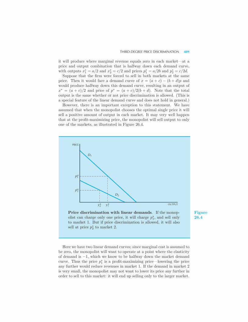
THIRD-DEGREE PRICE DISCRIMINATION 489
it will produce where marginal revenue equals zero in each market—at aprice and output combination that is halfway down each demand curve,with outputs x∗
1 = a/2 and x∗2 = c/2 and prices p∗1 = a/2b and p∗2 = c/2d.
Suppose that the firm were forced to sell in both markets at the sameprice. Then it would face a demand curve of x = (a + c) − (b + d)p andwould produce halfway down this demand curve, resulting in an output ofx∗ = (a + c)/2 and price of p∗ = (a + c)/2(b + d). Note that the totaloutput is the same whether or not price discrimination is allowed. (This isa special feature of the linear demand curve and does not hold in general.)However, there is an important exception to this statement. We have
assumed that when the monopolist chooses the optimal single price it willsell a positive amount of output in each market. It may very well happenthat at the profit-maximizing price, the monopolist will sell output to onlyone of the markets, as illustrated in Figure 26.4.
PRICE
D
p*
p*D
y *y * OUTPUT2
2
2
1
1
1
Price discrimination with linear demands. If the monop-olist can charge only one price, it will charge p∗1, and sell onlyto market 1. But if price discrimination is allowed, it will alsosell at price p∗2 to market 2.
Figure26.4
Here we have two linear demand curves; since marginal cost is assumed tobe zero, the monopolist will want to operate at a point where the elasticityof demand is −1, which we know to be halfway down the market demandcurve. Thus the price p∗1 is a profit-maximizing price—lowering the priceany further would reduce revenues in market 1. If the demand in market 2is very small, the monopolist may not want to lower its price any further inorder to sell to this market: it will end up selling only to the larger market.
490 MONOPOLY BEHAVIOR (Ch. 26)
In this case, allowing price discrimination will unambiguously increasetotal output, since the monopolist will find it in its interest to sell to bothmarkets if it can charge a different price in each one.
EXAMPLE: Calculating Optimal Price Discrimination
Suppose that a monopolist faces two markets with demand curves given by
D1(p1) = 100− p1
D2(p2) = 100− 2p2.
Assume that the monopolist’s marginal cost is constant at $20 a unit. If itcan price discriminate, what price should it charge in each market in orderto maximize profits? What if it can’t price discriminate? Then what priceshould it charge?To solve the price-discrimination problem, we first calculate the inverse
demand functions:p1(y1) = 100− y1
p2(y2) = 50− y2/2.
Marginal revenue equals marginal cost in each market yields the two equa-tions:
100− 2y1 = 20
50− y2 = 20.
Solving we have y∗1 = 40 and y∗2 = 30. Substituting back into the inversedemand functions gives us the prices p∗1 = 60 and p∗2 = 35.
If the monopolist must charge the same price in each market, we firstcalculate the total demand:
D(p) = D1(p1) +D2(p2) = 200− 3p.
The inverse demand curve is
p(y) =200
3− y
3.
Marginal revenue equals marginal cost gives us
200
3− 2
3y = 20,
which can be solved to give y∗ = 70 and p∗ = 43 13 .
In accord with the discussion in the previous section, it is importantto check that this price generates non-negative demands in each market.However, it is easily checked that this is the case.
THIRD-DEGREE PRICE DISCRIMINATION 491
EXAMPLE: Price Discrimination in Academic Journals
Most written scholarly communication takes place in academic journals.These journals are sold by subscription to libraries and to individual schol-ars. It is very common to see different subscription prices being charged tolibraries and individuals. In general, we would expect that the demand bylibraries would be much more inelastic than demand by individuals, and,just as economic analysis would predict, the prices for library subscriptionsare typically much higher than the prices for individual subscriptions. Of-ten library subscriptions are 2 to 3 times more expensive than subscriptionsto individuals.More recently, some publishers have begun to price discriminate by ge-
ography. During 1984, when the U.S. dollar was at an all-time high ascompared to the English pound, many British publishers began to chargedifferent prices to U.S. subscribers than to European subscribers. It wouldbe expected that the U.S. demand would be more inelastic. Since the dol-lar price of British journals was rather low due to the exchange rate, a 10percent increase in the U.S. price would result in a smaller percentage dropin demand than a similar increase in the British price. Thus, on groundsof profit maximization, it made sense for the British publishers to raise theprices of their journals to the group with the lower elasticity of demand—the U.S. subscribers. According to a 1984 study, North American librarieswere charged an average of 67 percent more for their journals than U.K.libraries, and 34 percent more than anyone else in the world.3
Further evidence for price discrimination can be found by examiningthe pattern of price increases. According to a study by the Universityof Michigan Library, “. . . publishers have carefully considered their newpricing strategy. There seems to be a direct correlation . . . between patternsof library usage and the magnitude of the pricing differential. The greaterthe use, the larger the differential.”4
By 1986 the exchange rate had turned in favor of the pound, and thedollar prices of the British journals had increased significantly. Along withthe price increase came some serious resistance to the higher prices. Theconcluding sentences of the Michigan report are illustrative: “One expectsthat a vendor with a monopoly on a product will charge according todemand. What the campus as a customer must determine is whether itwill continue to pay up to 114% more than its British counterparts for theidentical product.”
3 Hamaker, C. and Astle, D., “Recent Pricing Patterns in British Journal Publishing,”Library Acquisitions: Practice and Theory , 8, 4 (Spring 1984), 225–32.
4 The study was conducted by Robert Houbeck for the University of Michigan Library,and published in Vol. 2, No. 1 of the University Library Update, April 1986.
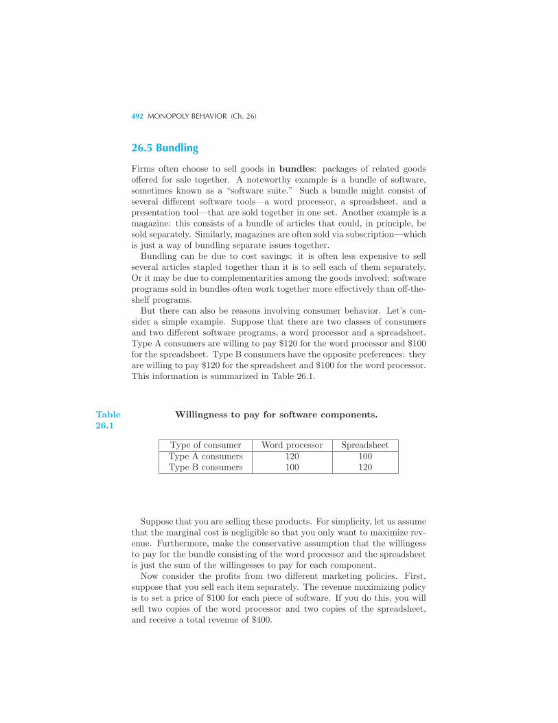
492 MONOPOLY BEHAVIOR (Ch. 26)
26.5 Bundling
Firms often choose to sell goods in bundles: packages of related goodsoffered for sale together. A noteworthy example is a bundle of software,sometimes known as a “software suite.” Such a bundle might consist ofseveral different software tools—a word processor, a spreadsheet, and apresentation tool—that are sold together in one set. Another example is amagazine: this consists of a bundle of articles that could, in principle, besold separately. Similarly, magazines are often sold via subscription—whichis just a way of bundling separate issues together.Bundling can be due to cost savings: it is often less expensive to sell
several articles stapled together than it is to sell each of them separately.Or it may be due to complementarities among the goods involved: softwareprograms sold in bundles often work together more effectively than off-the-shelf programs.But there can also be reasons involving consumer behavior. Let’s con-
sider a simple example. Suppose that there are two classes of consumersand two different software programs, a word processor and a spreadsheet.Type A consumers are willing to pay $120 for the word processor and $100for the spreadsheet. Type B consumers have the opposite preferences: theyare willing to pay $120 for the spreadsheet and $100 for the word processor.This information is summarized in Table 26.1.
Table26.1
Willingness to pay for software components.
Type of consumer Word processor SpreadsheetType A consumers 120 100Type B consumers 100 120
Suppose that you are selling these products. For simplicity, let us assumethat the marginal cost is negligible so that you only want to maximize rev-enue. Furthermore, make the conservative assumption that the willingessto pay for the bundle consisting of the word processor and the spreadsheetis just the sum of the willingesses to pay for each component.Now consider the profits from two different marketing policies. First,
suppose that you sell each item separately. The revenue maximizing policyis to set a price of $100 for each piece of software. If you do this, you willsell two copies of the word processor and two copies of the spreadsheet,and receive a total revenue of $400.
TWO-PART TARIFFS 493
But what if you bundle the items together? In this case, you could selleach bundle for $220, and receive a net revenue of $440. The bundlingstrategy is clearly more attractive!What is going on in this example? Recall that when you sell an item
to several different people, the price is determined by the purchaser whohas the lowest willingess to pay. The more diverse the valuations of theindividuals, the lower the price you have to charge to sell a given numberof items. In this case bundling the word processor and the spreadsheetreduces the dispersion of willingess to pay—allowing the monopolist to seta higher price for the bundle of goods.
EXAMPLE: Software Suites
Microsoft, Lotus, and other software manufacturers have taken to bundlingmuch of their applications software. For example, in 1993 Microsoft offereda spreadsheet, word processor, presentation tool, and database as the “Mi-crosoft Office” package at a suggested retail price of $750. (The discounted“street price” was about $450.) If bought separately, the individual soft-ware applications would total $1,565! Lotus offered its “Smart Suite” atessentially the same price; its separate components sold for a total of $1,730.According to an article by Steve Lohr in the October 15, 1993, New York
Times, 50 percent of Microsoft’s applications software was sold in bundles,and generated revenue of over $1 billion a year.These software suites fit the bundling model well. Tastes for software are
often very heterogeneous. Some people use a word processor every day anduse a spreadsheet only occasionally. Other people have the reverse patternof software use. If you wish to sell a spreadsheet to a large number ofusers, you have to sell it at a price that will be attractive to an occasionaluser. Similarly with the word processor: it is the willingness to pay of themarginal user that sets the market price. By bundling the two productstogether, the dispersion of willingnesses to pay is reduced and total profitscan increase.This is not to say that bundling is the whole story in software suites;
other phenomena are also at work. The individual components of thesuites are guaranteed to work well together; they are complementary goodsin this respect. Furthermore, the success of a piece of software tends todepend strongly on how many people use it, and bundling software helpsto build market share. We will investigate this phenomenon of networkexternalities in Chapter 36.
26.6 Two-Part Tariffs
Consider the pricing problem facing the owners of an amusement park.They can set one price for tickets to get into the park and another price for
494 MONOPOLY BEHAVIOR (Ch. 26)
the rides. How should they set these two prices if they want to maximizeprofits? Note that the demand for access and the demand for rides areinterrelated: the price that people are willing to pay to get into the parkwill depend on the price that they have to pay for the rides. This kind oftwo-part pricing scheme is known as a two-part tariff.5
Other applications of two-part tariffs abound: Polaroid sells its camerafor one price and its film for another. People who are deciding whetheror not to purchase the camera presumably consider the price of the film.A company that makes razor blades sells the razor for one price and theblades for another—again the price they set for the blades influences thedemand for razors and vice versa.Let us consider how to solve this pricing problem in the context of the
original example: the so-called Disneyland Dilemma. As usual we willmake some simplifying assumptions. First, we assume that there is onlyone kind of ride in Disneyland. Second, we assume that people only desireto go to Disneyland for the rides. Finally, we assume that everyone has thesame tastes for rides.In Figure 26.5 we have depicted the demand curve and the (constant)
marginal cost curve for rides. As usual the demand curve slopes down—ifDisney sets a high price for each ride, fewer rides will be taken. Supposethat they set a price of p∗, as in Figure 26.5, that leads to a demand forx∗ rides. How much will they be able to charge for admission to the park,given that the rides cost p∗?
The total willingness to pay for x∗ rides is measured by the consumers’surplus. Hence the most that the owners of the park can charge for admis-sion is the area labeled “consumer’s surplus” in Figure 26.5. The total prof-its to the monopolist is this area plus the profit on the rides, (p∗−MC)x∗.
It is not hard to see that total profits are maximized when price equalsmarginal cost: we’ve seen before that this price gives the largest possibleconsumer plus producer surplus. Since the monopolist gets to charge peopletheir consumers’ surplus, setting price equal to marginal cost and the entryfee to the resulting consumer’s surplus is the profit-maximizing policy.Indeed, this is the policy that Disneyland, and most other amusement
parks follow. There is one price for admission, but then the attractionsinside are free. It appears that the marginal cost of the rides is less thanthe transactions cost of collecting a separate payment for them.
26.7 Monopolistic Competition
We have described a monopolistic industry as being one in which there is asingle large producer. But we’ve been somewhat vague about exactly what
5 See the classic article by Walter Oi, “A Disneyland Dilemma: Two-Part Tariffs for aMickey Mouse Monopoly,” Quarterly Journal of Economics, 85 (1971), 77–96.
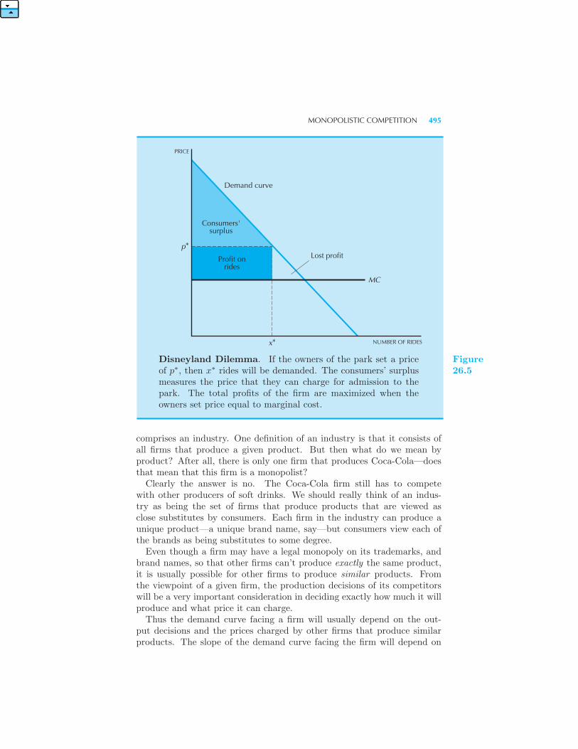
MONOPOLISTIC COMPETITION 495
Lost profitProfit onrides
Consumers'surplus
Demand curve
PRICE
p*
NUMBER OF RIDESx*
MC
Disneyland Dilemma. If the owners of the park set a priceof p∗, then x∗ rides will be demanded. The consumers’ surplusmeasures the price that they can charge for admission to thepark. The total profits of the firm are maximized when theowners set price equal to marginal cost.
Figure26.5
comprises an industry. One definition of an industry is that it consists ofall firms that produce a given product. But then what do we mean byproduct? After all, there is only one firm that produces Coca-Cola—doesthat mean that this firm is a monopolist?Clearly the answer is no. The Coca-Cola firm still has to compete
with other producers of soft drinks. We should really think of an indus-try as being the set of firms that produce products that are viewed asclose substitutes by consumers. Each firm in the industry can produce aunique product—a unique brand name, say—but consumers view each ofthe brands as being substitutes to some degree.Even though a firm may have a legal monopoly on its trademarks, and
brand names, so that other firms can’t produce exactly the same product,it is usually possible for other firms to produce similar products. Fromthe viewpoint of a given firm, the production decisions of its competitorswill be a very important consideration in deciding exactly how much it willproduce and what price it can charge.Thus the demand curve facing a firm will usually depend on the out-
put decisions and the prices charged by other firms that produce similarproducts. The slope of the demand curve facing the firm will depend on
496 MONOPOLY BEHAVIOR (Ch. 26)
how similar the other firms’ products are. If a large number of the firmsin the industry produce identical products, then the demand curve facingany one of them will be essentially flat. Each firm must sell its product forwhatever price the other firms are charging. Any firm that tried to raiseits price above the prices of the other firms selling identical products wouldsoon lose all of its customers.On the other hand, if one firm has the exclusive rights to sell a particular
product, then it may be able to raise its price without losing all of itscustomers. Some, but not all, of its customers may switch to competitors’products. Just how many customers switch depends on how similar thecustomers think the products are—that is, on the elasticity of the demandcurve facing the firm.
If a firm is making a profit selling a product in an industry, and otherfirms are not allowed to perfectly reproduce that product, they still mayfind it profitable to enter that industry and produce a similar but distinctiveproduct. Economists refer to this phenomenon as product differentia-tion—each firm attempts to differentiate its product from the other firmsin the industry. The more successful it is at differentiating its product fromother firms selling similar products, the more monopoly power it has—thatis, the less elastic is the demand curve for the product. For example,consider the soft drink industry. In this industry there are a number offirms producing similar, but not identical products. Each product has itsfollowing of consumers, and so has some degree of market power.
An industry structure such as that described above shares elements ofboth competition and monopoly; it is therefore referred to asmonopolisticcompetition. The industry structure is monopolistic in that each firmfaces a downward-sloping demand curve for its product. It therefore hassome market power in the sense that it can set its own price, rather thanpassively accept the market price as does a competitive firm. On the otherhand the firms must compete for customers in terms of both price and thekinds of products they sell. Furthermore, there are no restrictions againstnew firms entering into a monopolistically competitive industry. In theseaspects the industry is like a competitive industry.
Monopolistic competition is probably the most prevalent form of industrystructure. Unfortunately, it is also the most difficult form to analyze. Theextreme cases of pure monopoly and pure competition are much simplerand can often be used as first approximations to more elaborate models ofmonopolistic competition. In a detailed model of a monopolistically com-petitive industry, much depends on the specific details of the products andtechnology, as well as on the nature of the strategic choices available tofirms. It is unreasonable to model a monopolistically competitive industryin the abstract, as we have done with the simpler cases of pure competi-tion and pure monopoly. Rather, the institutional details of the particularindustry under consideration must be examined. We will describe somemethods that economists use to analyze strategic choice in the next two
MONOPOLISTIC COMPETITION 497
chapters, but a detailed study of monopolistic competition will have to waitfor more advanced courses.We can, however, describe an interesting feature of the free entry aspect
of monopolistic competition. As more and more firms enter the industryfor a particular kind of product, how would we expect the demand curveof an incumbent firm to change? First, we would expect the demand curveto shift inward since we would expect that at each price, it would sell fewerunits of output as more firms enter the industry. Second, we would expectthat the demand curve facing a given firm would become more elastic asmore firms produced more and more similar products. Thus entry into anindustry by new firms with similar products will tend to shift the demandcurves facing existing firms to the left and make them flatter.If firms continue to enter the industry as long as they expect to make a
profit, equilibrium must satisfy the following three conditions:
1. Each firm is selling at a price and output combination on its demandcurve.
2. Each firm is maximizing its profits, given the demand curve facing it.
3. Entry has forced the profits of each firm down to zero.
These facts imply a very particular geometrical relationship between thedemand curve and the average cost curve: the demand curve and the av-erage cost curve must be tangent to each other.The argument is illustrated in Figure 26.6. Fact 1 says that the output
and price combination must be somewhere on the demand curve, and fact3 says that the output and price combination must also be on the averagecost curve. Thus the operating position of the firm must be at a point thatlies on both curves. Could the demand curve cross the average cost curve?No, because then there would be some point on the demand curve abovethe average cost curve—but this would be a point yielding positive profits.6
And by fact 2, the zero profit point is a profit maximum.Another way to see this is to examine what would happen if the firm
depicted in Figure 26.6 charged any price other than the break-even price.At any other price, higher or lower, the firm would lose money, while at thebreak-even price, the firm makes zero profits. Thus the break-even price isthe profit-maximizing price.There are two worthwhile observations about the monopolistically com-
petitive equilibrium. First, although profits are zero, the situation is stillPareto inefficient. Profits have nothing to do with the efficiency question:when price is greater than marginal cost, there is an efficiency argumentfor expanding output.
6 If p > c(y)/y, then simple algebra shows that py − c(y) > 0.
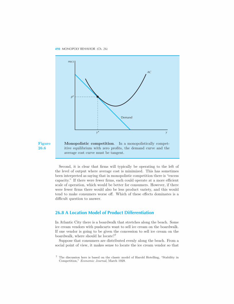
498 MONOPOLY BEHAVIOR (Ch. 26)
PRICE
p*
AC
Demand
y* y
Figure26.6
Monopolistic competition. In a monopolistically compet-itive equilibrium with zero profits, the demand curve and theaverage cost curve must be tangent.
Second, it is clear that firms will typically be operating to the left ofthe level of output where average cost is minimized. This has sometimesbeen interpreted as saying that in monopolistic competition there is “excesscapacity.” If there were fewer firms, each could operate at a more efficientscale of operation, which would be better for consumers. However, if therewere fewer firms there would also be less product variety, and this wouldtend to make consumers worse off. Which of these effects dominates is adifficult question to answer.
26.8 A Location Model of Product Differentiation
In Atlantic City there is a boardwalk that stretches along the beach. Someice cream vendors with pushcarts want to sell ice cream on the boardwalk.If one vendor is going to be given the concession to sell ice cream on theboardwalk, where should he locate?7
Suppose that consumers are distributed evenly along the beach. From asocial point of view, it makes sense to locate the ice cream vendor so that
7 The discussion here is based on the classic model of Harold Hotelling, “Stability inCompetition,” Economic Journal, March 1929.
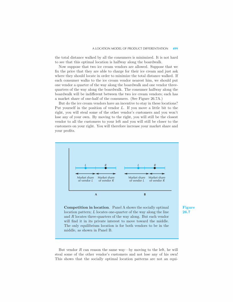
A LOCATION MODEL OF PRODUCT DIFFERENTIATION 499
the total distance walked by all the consumers is minimized. It is not hardto see that this optimal location is halfway along the boardwalk.Now suppose that two ice cream vendors are allowed. Suppose that we
fix the price that they are able to charge for their ice cream and just askwhere they should locate in order to minimize the total distance walked. Ifeach consumer walks to the ice cream vendor nearest him, we should putone vendor a quarter of the way along the boardwalk and one vendor three-quarters of the way along the boardwalk. The consumer halfway along theboardwalk will be indifferent between the two ice cream vendors; each hasa market share of one-half of the consumers. (See Figure 26.7A.)But do the ice cream vendors have an incentive to stay in these locations?
Put yourself in the position of vendor L. If you move a little bit to theright, you will steal some of the other vendor’s customers and you won’tlose any of your own. By moving to the right, you will still be the closestvendor to all the customers to your left and you will still be closer to thecustomers on your right. You will therefore increase your market share andyour profits.
L R L R
Market shareof vendor R
Market shareof vendor L
Market shareof vendor R
Market shareof vendor L
A B
Competition in location. Panel A shows the socially optimallocation pattern; L locates one-quarter of the way along the lineand R locates three-quarters of the way along. But each vendorwill find it in its private interest to move toward the middle.The only equilibrium location is for both vendors to be in themiddle, as shown in Panel B.
Figure26.7
But vendor R can reason the same way—by moving to the left, he willsteal some of the other vendor’s customers and not lose any of his own!This shows that the socially optimal location patterns are not an equi-
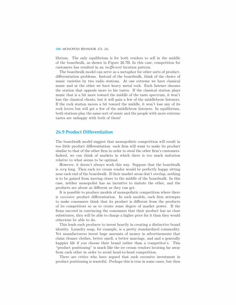
500 MONOPOLY BEHAVIOR (Ch. 26)
librium. The only equilibrium is for both vendors to sell in the middleof the boardwalk, as shown in Figure 26.7B. In this case, competition forcustomers has resulted in an inefficient location pattern.The boardwalk model can serve as a metaphor for other sorts of product-
differentiation problems. Instead of the boardwalk, think of the choice ofmusic varieties by two radio stations. At one extreme we have classicalmusic and at the other we have heavy metal rock. Each listener choosesthe station that appeals more to his tastes. If the classical station playsmusic that is a bit more toward the middle of the taste spectrum, it won’tlose the classical clients, but it will gain a few of the middlebrow listeners.If the rock station moves a bit toward the middle, it won’t lose any of itsrock lovers but will get a few of the middlebrow listeners. In equilibrium,both stations play the same sort of music and the people with more extremetastes are unhappy with both of them!
26.9 Product Differentiation
The boardwalk model suggest that monopolistic competition will result intoo little product differentiation: each firm will want to make its productsimilar to that of the other firm in order to steal the other firm’s customers.Indeed, we can think of markets in which there is too much imitationrelative to what seems to be optimal.However, it doesn’t always work this way. Suppose that the boardwalk
is very long. Then each ice cream vendor would be perfectly happy sittingnear each end of the boardwalk. If their market areas don’t overlap, nothingis to be gained from moving closer to the middle of the boardwalk. In thiscase, neither monopolist has an incentive to imitate the other, and theproducts are about as different as they can get.It is possible to produce models of monopolistic competition where there
is excessive product differentiation. In such models, each firm attemptsto make consumers think that its product is different from the productsof its competitors so as to create some degree of market power. If thefirms succeed in convincing the consumers that their product has no closesubstitutes, they will be able to charge a higher price for it than they wouldotherwise be able to do.This leads each producer to invest heavily in creating a distinctive brand
identity. Laundry soap, for example, is a pretty standardized commodity.Yet manufacturers invest huge amounts of money in advertisements thatclaim cleaner clothes, better smell, a better marriage, and and a generallyhappier life if you choose their brand rather than a competitor’s. This“product positioning” is much like the ice cream vendors locating far awayfrom each other in order to avoid head-to-head competition.There are critics who have argued that such excessive investment in
product positioning is wasteful. Perhaps this is true in some cases, but then
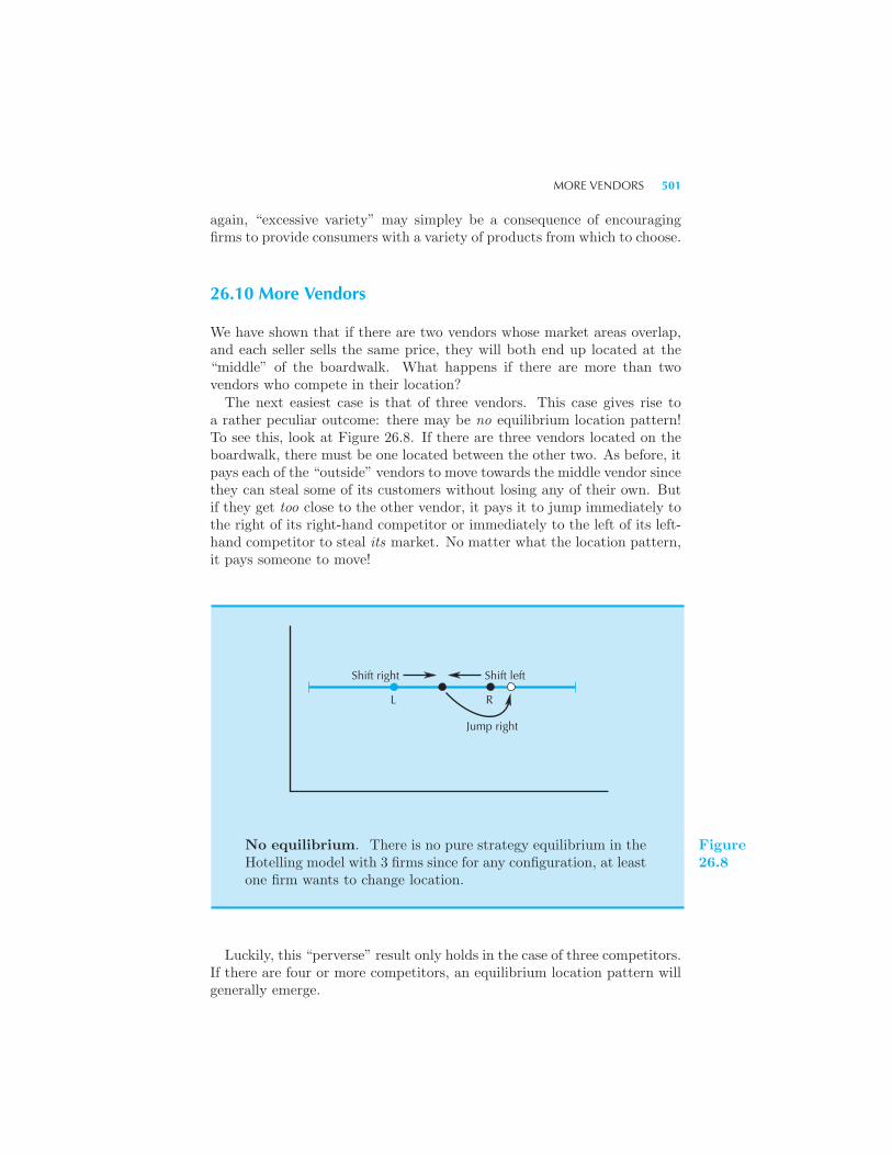
MORE VENDORS 501
again, “excessive variety” may simpley be a consequence of encouragingfirms to provide consumers with a variety of products from which to choose.
26.10 More Vendors
We have shown that if there are two vendors whose market areas overlap,and each seller sells the same price, they will both end up located at the“middle” of the boardwalk. What happens if there are more than twovendors who compete in their location?The next easiest case is that of three vendors. This case gives rise to
a rather peculiar outcome: there may be no equilibrium location pattern!To see this, look at Figure 26.8. If there are three vendors located on theboardwalk, there must be one located between the other two. As before, itpays each of the “outside” vendors to move towards the middle vendor sincethey can steal some of its customers without losing any of their own. Butif they get too close to the other vendor, it pays it to jump immediately tothe right of its right-hand competitor or immediately to the left of its left-hand competitor to steal its market. No matter what the location pattern,it pays someone to move!
L R
Shift right Shift left
Jump right
No equilibrium. There is no pure strategy equilibrium in theHotelling model with 3 firms since for any configuration, at leastone firm wants to change location.
Figure26.8
Luckily, this “perverse” result only holds in the case of three competitors.If there are four or more competitors, an equilibrium location pattern willgenerally emerge.
502 MONOPOLY BEHAVIOR (Ch. 26)
Summary
1. There will typically be an incentive for a monopolist to engage in pricediscrimination of some sort.
2. Perfect price discrimination involves charging each customer a differenttake-it-or-leave-it price. This will result in an efficient level of output.
3. If a firm can charge different prices in two different markets, it will tendto charge the lower price in the market with the more elastic demand.
4. If a firm can set a two-part tariff, and consumers are identical, then itwill generally want to set price equal to marginal cost and make all of itsprofits from the entry fee.
5. The industry structure known as monopolistic competition refers to asituation in which there is product differentiation, so each firm has somedegree of monopoly power, but there is also free entry so that profits aredriven to zero.
6. Monopolistic competition can result in too much or too little productdifferentiation in general.
REVIEW QUESTIONS
1. Will a monopoly ever provide a Pareto efficient level of output on itsown?
2. Suppose that a monopolist sells to two groups that have constant elas-ticity demand curves, with elasticity ε1 and ε2. The marginal cost of pro-duction is constant at c. What price is charged to each group?
3. Suppose that the amusement park owner can practice perfect first-degreeprice discrimination by charging a different price for each ride. Assume thatall rides have zero marginal cost and all consumers have the same tastes.Will the monopolist do better charging for rides and setting a zero pricefor admission, or better by charging for admission and setting a zero pricefor rides?
4. Disneyland also offers a discount on admissions to residents of SouthernCalifornia. (You show them your zip code at the gate.) What kind ofprice discrimination is this? What does this imply about the elasticity ofdemand for Disney attractions by Southern Californians?
CHAPTER 27
FACTORMARKETS
In our examination of factor demands in Chapter 20 we only consideredthe case of a firm that faced a competitive output market and a competi-tive factor market. Now that we have studied monopoly behavior, we canexamine some alternative specifications of factor demand behavior. For ex-ample, what happens to factor demands if a firm behaves as a monopolistin its output market? Or what happens to factor demands if a firm is thesole demander for the use of some factors? We investigate these questionsand some related questions in this chapter.
27.1 Monopoly in the Output Market
When a firm determines its profit-maximizing demand for a factor, it willalways want to choose a quantity such that the marginal revenue fromhiring a little more of that factor just equals the marginal cost of doingso. This follows from the standard logic: if the marginal revenue of someaction didn’t equal the marginal cost of that action, then it would pay forthe firm to change the action.
504 FACTOR MARKETS (Ch. 27)
This general rule takes various special forms depending on our assump-tions about the environment in which the firm operates. For example,suppose that the firm has a monopoly for its output. For simplicity we willsuppose that there is only one factor of production and write the produc-tion function as y = f(x). The revenue that the firm receives depends onits production of output so we write R(y) = p(y)y, where p(y) is the inversedemand function. Let us see how a marginal increase in the amount of theinput affects the revenues of the firm.Suppose that we increase the amount of the input a little bit, Δx. This
will result in a small increase in output, Δy. The ratio of the increase inoutput to the increase in the input is the marginal product of the factor:
MPx =Δy
Δx=
f(x+Δx)− f(x)
Δx. (27.1)
This increase in output will cause revenue to change. The change inrevenue is called the marginal revenue.
MRy =ΔR
Δy=
R(y +Δy)−R(y)
Δy. (27.2)
The effect on revenue due to the marginal increase in the input is calledthe marginal revenue product. Examining equations (27.1) and (27.2)we see that it is given by
MRPx =ΔR
Δx=
ΔR
Δy
Δy
Δx
= MRy ×MPx.
We can use our standard expression for marginal revenue to write this as
MRPx =
[p(y) +
Δp
Δyy
]MPx
= p(y)
[1 +
1
ε
]MPx
= p(y)
[1− 1
|ε|
]MPx.
The first expression is the usual expression for marginal revenue. Thesecond and third expressions use the elasticity form of marginal revenue,which was discussed in Chapter 15.Now it is easy to see how this generalizes the competitive case we ex-
amined earlier in Chapter 20. The elasticity of the demand curve facingan individual firm in a competitive market is infinite; consequently themarginal revenue for a competitive firm is just equal to price. Hence the
MONOPOLY IN THE OUTPUT MARKET 505
“marginal revenue product” of an input for a firm in a competitive marketis just the value of the marginal product of that input, pMPx.
How does the marginal revenue product (in the case of a monopoly)compare to the value of the marginal product? Since the demand curvehas a negative slope, we see that the marginal revenue product will alwaysbe less than the value of the marginal product:
MRPx = p
[1− 1
|ε|
]MPx ≤ pMPx.
As long as the demand function is not perfectly elastic, the MRPx will bestrictly less than pMPx. This means that at any level of employment ofthe factor, the marginal value of an additional unit is less for a monopolistthan for a competitive firm. In the rest of this section we will assume thatwe are dealing with this case—the case where the monopolist actually hassome monopoly power.At first encounter this statement seems paradoxical since a monopolist
makes higher profits than a competitive firm. In this sense the total factorinput is “worth more” to a monopolist than to a competitive firm.The resolution of this “paradox” is to note the difference between total
value and marginal value. The total amount employed of the factor isindeed worth more to the monopolist than to the competitive firm sincethe monopolist will make more profits from the factor than the competitivefirm. However, at a given level of output an increase in the employmentof the factor will increase output and reduce the price that a monopolistis able to charge. But an increase in a competitive firm’s output will notchange the price it can charge. Thus on the margin, a small increase inthe employment of the factor is worth less to the monopolist than to thecompetitive firm.Since increases in the factor employment are worth less to a monopo-
list than to a competitive firm on the margin in the short run, it makessense that the monopolist would usually want to employ less of the input.Indeed this is generally true: the monopolist increases its profits by reduc-ing its output, and so it will usually hire lower amounts of inputs than acompetitive firm.In order to determine how much of the factor a firm employs, we have
to compare the marginal revenue of an additional unit of the factor to themarginal cost of hiring that factor. Let us assume that the firm operatesin a competitive factor market, so that it can hire as much of the factor asit wants at a constant price of w. In this case, the competitive firm wantsto hire xc units of the factor, where
pMP (xc) = w.
The monopolist, on the other hand, wants to hire xm units of the factor,where
MRP (xm) = w.
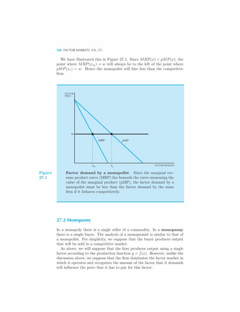
506 FACTOR MARKETS (Ch. 27)
We have illustrated this in Figure 27.1. Since MRP (x) < pMP (x), thepoint where MRP (xm) = w will always be to the left of the point wherepMP (xc) = w. Hence the monopolist will hire less than the competitivefirm.
FACTORPRICE
w
MRP pMP
x x FACTOR DEMANDm c
Figure27.1
Factor demand by a monopolist. Since the marginal rev-enue product curve (MRP) lies beneath the curve measuring thevalue of the marginal product (pMP), the factor demand by amonopolist must be less than the factor demand by the samefirm if it behaves competitively.
27.2 Monopsony
In a monopoly there is a single seller of a commodity. In a monopsonythere is a single buyer. The analysis of a monopsonist is similar to that ofa monopolist. For simplicity, we suppose that the buyer produces outputthat will be sold in a competitive market.As above, we will suppose that the firm produces output using a single
factor according to the production function y = f(x). However, unlike thediscussion above, we suppose that the firm dominates the factor market inwhich it operates and recognizes the amount of the factor that it demandswill influence the price that it has to pay for this factor.
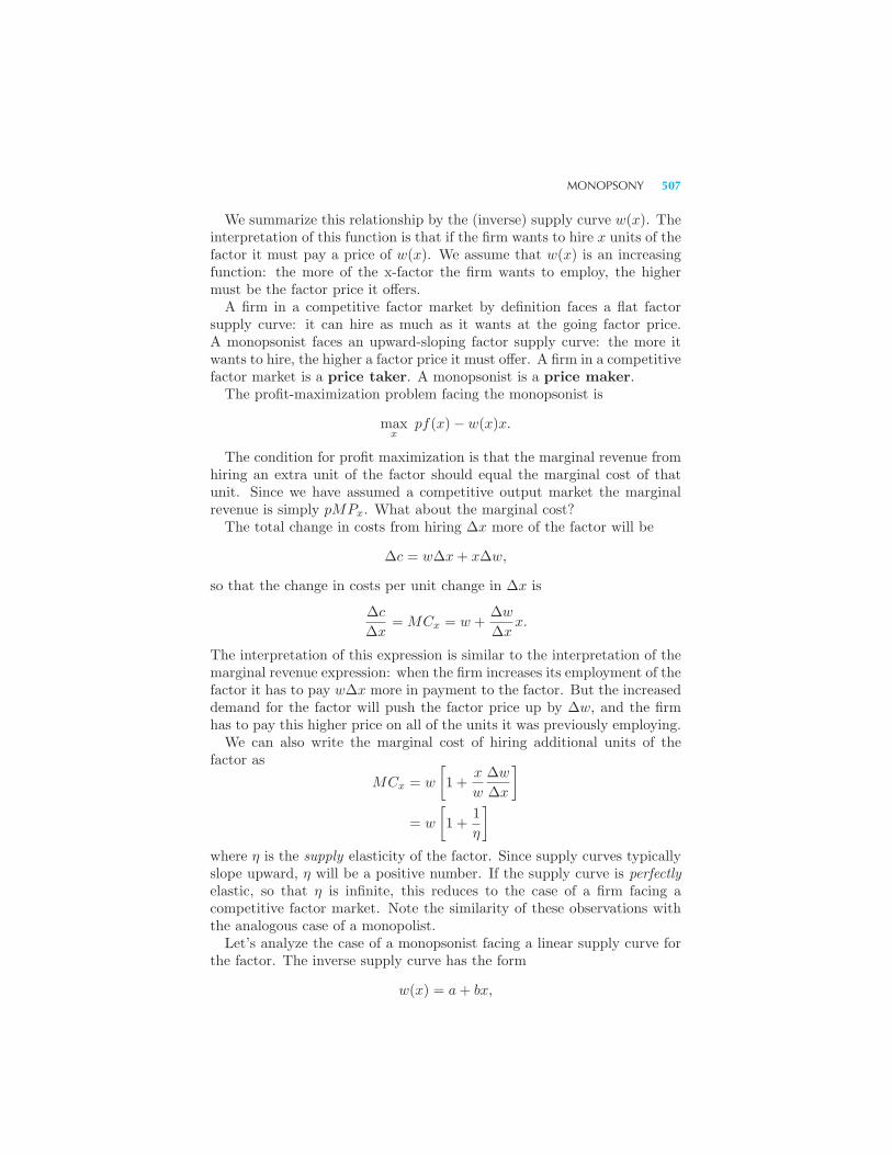
MONOPSONY 507
We summarize this relationship by the (inverse) supply curve w(x). Theinterpretation of this function is that if the firm wants to hire x units of thefactor it must pay a price of w(x). We assume that w(x) is an increasingfunction: the more of the x-factor the firm wants to employ, the highermust be the factor price it offers.A firm in a competitive factor market by definition faces a flat factor
supply curve: it can hire as much as it wants at the going factor price.A monopsonist faces an upward-sloping factor supply curve: the more itwants to hire, the higher a factor price it must offer. A firm in a competitivefactor market is a price taker. A monopsonist is a price maker.The profit-maximization problem facing the monopsonist is
maxx
pf(x)− w(x)x.
The condition for profit maximization is that the marginal revenue fromhiring an extra unit of the factor should equal the marginal cost of thatunit. Since we have assumed a competitive output market the marginalrevenue is simply pMPx. What about the marginal cost?The total change in costs from hiring Δx more of the factor will be
Δc = wΔx+ xΔw,
so that the change in costs per unit change in Δx is
Δc
Δx= MCx = w +
Δw
Δxx.
The interpretation of this expression is similar to the interpretation of themarginal revenue expression: when the firm increases its employment of thefactor it has to pay wΔx more in payment to the factor. But the increaseddemand for the factor will push the factor price up by Δw, and the firmhas to pay this higher price on all of the units it was previously employing.We can also write the marginal cost of hiring additional units of the
factor as
MCx = w
[1 +
x
w
Δw
Δx
]
= w
[1 +
1
η
]
where η is the supply elasticity of the factor. Since supply curves typicallyslope upward, η will be a positive number. If the supply curve is perfectlyelastic, so that η is infinite, this reduces to the case of a firm facing acompetitive factor market. Note the similarity of these observations withthe analogous case of a monopolist.Let’s analyze the case of a monopsonist facing a linear supply curve for
the factor. The inverse supply curve has the form
w(x) = a+ bx,
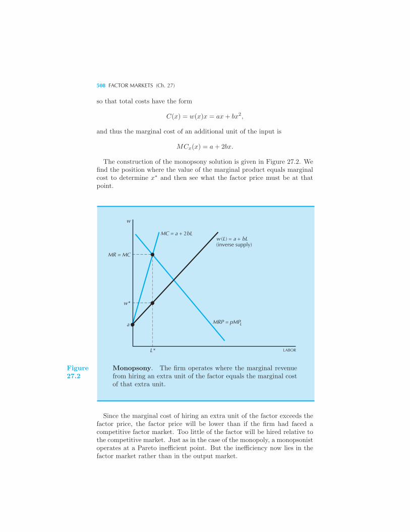
508 FACTOR MARKETS (Ch. 27)
so that total costs have the form
C(x) = w(x)x = ax+ bx2,
and thus the marginal cost of an additional unit of the input is
MCx(x) = a+ 2bx.
The construction of the monopsony solution is given in Figure 27.2. Wefind the position where the value of the marginal product equals marginalcost to determine x∗ and then see what the factor price must be at thatpoint.
MC = a + 2bL
MR = MC
w (L) = a + bL(inverse supply)
MRP = pMP
LABORL*
a
w*
L
w
Figure27.2
Monopsony. The firm operates where the marginal revenuefrom hiring an extra unit of the factor equals the marginal costof that extra unit.
Since the marginal cost of hiring an extra unit of the factor exceeds thefactor price, the factor price will be lower than if the firm had faced acompetitive factor market. Too little of the factor will be hired relative tothe competitive market. Just as in the case of the monopoly, a monopsonistoperates at a Pareto inefficient point. But the inefficiency now lies in thefactor market rather than in the output market.
MONOPSONY 509
EXAMPLE: The Minimum Wage
Suppose that the labor market is competitive and that the governmentsets a minimum wage that is higher than the prevailing equilibrium wage.Since demand equals supply at the equilibrium wage, the supply of laborwill exceed the demand for labor at the higher minimum wage. This isdepicted in Figure 27.3A.
WAGE
S
D
LABORLL
w
w
MCS
LABOR
D
w
w
LL
c
cmw m c
c
m
L
WAGE
A B
Minimum wage. Panel A shows the effect of a minimum wagein a competitive labor market. At the competitive wage, wc, em-ployment would be Lc. At the minimum wage, w, employmentis only Lmw. Panel B shows the effect of a minimum wage ina monopsonized labor market. Under monopsony, the wage iswm and employment is Lm, which is less than the employmentin the competitive labor market. If the minimum wage is set towc, employment will increase to Lc.
Figure27.3
Things are very different if the labor market is dominated by a monop-sonist. In this case, it is possible that imposing a minimum wage mayactually increase employment. This is depicted in Figure 27.3B. If thegovernment sets the minimum wage equal to the wage that would prevailin a competitive market, the “monopsonist” now perceives that it can hireworkers at a constant wage of wc. Since the wage rate it faces is now in-dependent of how many workers it hires, it will hire until the value of themarginal product equals wc. That is, it will hire just as many workers asif it faced a competitive labor market.Setting a wage floor for a monopsonist is just like setting a price ceiling
for a monopolist; each policy makes the firm behave as though it faced acompetitive market.
510 FACTOR MARKETS (Ch. 27)
27.3 Upstream and Downstream Monopolies
We have now examined two cases involving imperfect competition and fac-tor markets: the case of a firm with a monopoly in the output market butfacing a competitive factor market, and the case of a firm with a com-petitive output market that faces a monopolized factor market. Othervariations are possible. The firm could face a monopoly seller in its factormarket for example. Or it could face a monopsony buyer in its outputmarket. It doesn’t make much sense to plod through each possible case;they quickly become repetitive. However, we will examine one interestingmarket structure in which a monopoly produces output that is used as afactor of production by another monopolist.Suppose then that one monopolist produces output x at a constant mar-
ginal cost of c. We call this monopolist the upstream monopolist. Itsells the x-factor to another monopolist, the downstream monopolistat a price of k. The downstream monopolist uses the x-factor to produceoutput y according to the production function y = f(x). This output isthen sold in a monopolist market in which the inverse demand curve isp(y). For purposes of this example, we consider a linear inverse demandcurve p(y) = a− by.To make things simple, think of the production function as just being
y = x, so that for each unit of the x-input, the monopolist can produce oneunit of the y-output. We further suppose that the downstream monopolisthas no costs of production other than the unit price k that it must pay tothe upstream monopolist.In order to see how this market works, start with the downstream mo-
nopolist. Its profit-maximization problem is
maxy
p(y)y − ky = [a− by]y − ky.
Setting marginal revenue equal to marginal cost, we have
a− 2by = k,
which implies that
y =a− k
2b.
Since the monopolist demands one unit of the x-input for each y-outputthat it produces, this expression also determines the factor demand function
x =a− k
2b. (27.3)
This function tells us the relationship between the factor price k and theamount of the factor that the downstream monopolist will demand.
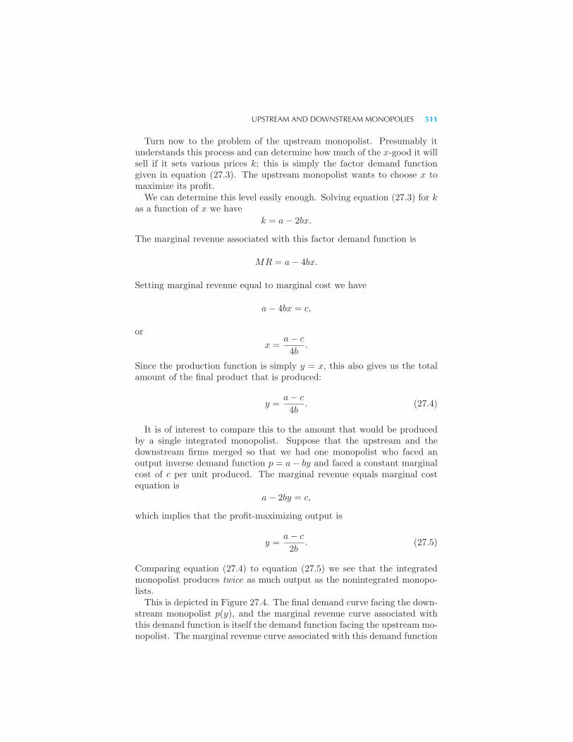
UPSTREAM AND DOWNSTREAM MONOPOLIES 511
Turn now to the problem of the upstream monopolist. Presumably itunderstands this process and can determine how much of the x-good it willsell if it sets various prices k; this is simply the factor demand functiongiven in equation (27.3). The upstream monopolist wants to choose x tomaximize its profit.We can determine this level easily enough. Solving equation (27.3) for k
as a function of x we have
k = a− 2bx.
The marginal revenue associated with this factor demand function is
MR = a− 4bx.
Setting marginal revenue equal to marginal cost we have
a− 4bx = c,
or
x =a− c
4b.
Since the production function is simply y = x, this also gives us the totalamount of the final product that is produced:
y =a− c
4b. (27.4)
It is of interest to compare this to the amount that would be producedby a single integrated monopolist. Suppose that the upstream and thedownstream firms merged so that we had one monopolist who faced anoutput inverse demand function p = a− by and faced a constant marginalcost of c per unit produced. The marginal revenue equals marginal costequation is
a− 2by = c,
which implies that the profit-maximizing output is
y =a− c
2b. (27.5)
Comparing equation (27.4) to equation (27.5) we see that the integratedmonopolist produces twice as much output as the nonintegrated monopo-lists.This is depicted in Figure 27.4. The final demand curve facing the down-
stream monopolist p(y), and the marginal revenue curve associated withthis demand function is itself the demand function facing the upstream mo-nopolist. The marginal revenue curve associated with this demand function
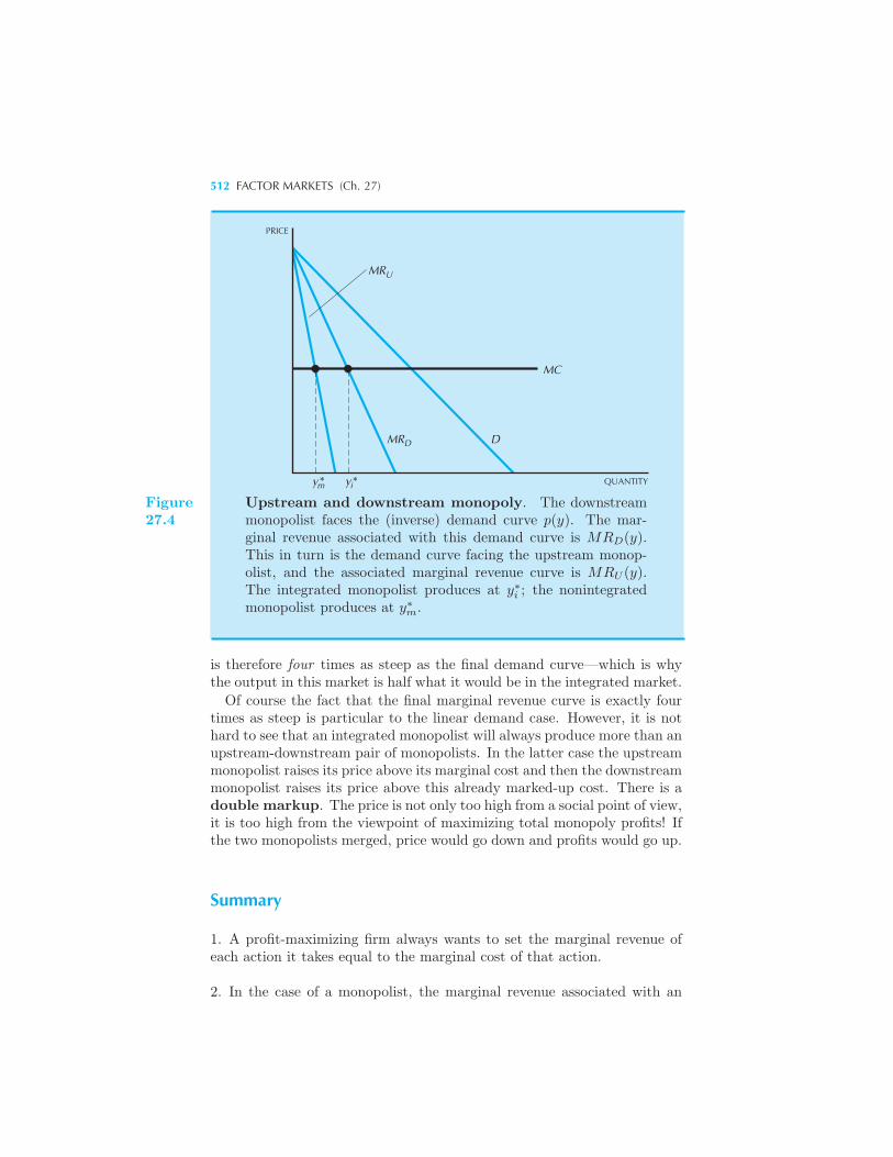
512 FACTOR MARKETS (Ch. 27)
PRICE
MR
MC
MR D
U
D
QUANTITYy ** ym i
Figure27.4
Upstream and downstream monopoly. The downstreammonopolist faces the (inverse) demand curve p(y). The mar-ginal revenue associated with this demand curve is MRD(y).This in turn is the demand curve facing the upstream monop-olist, and the associated marginal revenue curve is MRU (y).The integrated monopolist produces at y∗i ; the nonintegratedmonopolist produces at y∗m.
is therefore four times as steep as the final demand curve—which is whythe output in this market is half what it would be in the integrated market.
Of course the fact that the final marginal revenue curve is exactly fourtimes as steep is particular to the linear demand case. However, it is nothard to see that an integrated monopolist will always produce more than anupstream-downstream pair of monopolists. In the latter case the upstreammonopolist raises its price above its marginal cost and then the downstreammonopolist raises its price above this already marked-up cost. There is adouble markup. The price is not only too high from a social point of view,it is too high from the viewpoint of maximizing total monopoly profits! Ifthe two monopolists merged, price would go down and profits would go up.
Summary
1. A profit-maximizing firm always wants to set the marginal revenue ofeach action it takes equal to the marginal cost of that action.
2. In the case of a monopolist, the marginal revenue associated with an
APPENDIX 513
increase in the employment of a factor is called the marginal revenue prod-uct.
3. For a monopolist, the marginal revenue product will always be smallerthan the value of the marginal product due to the fact that the marginalrevenue from increasing output is always less than price.
4. Just as a monopoly consists of a market with a single seller, a monopsonyconsists of a market with a single buyer.
5. For a monopsonist the marginal cost curve associated with a factor willbe steeper than the supply curve of that factor.
6. Hence a monopsonist will hire an inefficiently small amount of the factorof production.
7. If an upstream monopolist sells a factor to a downstream monopolist,then the final price of output will be too high due to the double markupphenomenon.
REVIEW QUESTIONS
1. We saw that a monopolist never produced where the demand for outputwas inelastic. Will a monopsonist produce where a factor is inelasticallysupplied?
2. In our example of the minimum wage, what would happen if the labormarket was dominated by a monopsonist and the government set a wagethat was above the competitive wage?
3. In our examination of the upstream and downstream monopolists we de-rived expressions for the total output produced. What are the appropriateexpressions for the equilibrium prices, p and k?
APPENDIX
We can calculate marginal revenue product by using the chain rule. Let y = f(x)be the production function and p(y) be the inverse demand function. Revenueas a function of the factor employment is just
R(x) = p(f(x))f(x).
514 FACTOR MARKETS (Ch. 27)
Differentiating this expression with respect to x we have
dR(x)
dx= p(y)f ′(x) + f(x)p′(y)f ′(x)
= [p(y) + p′(y)y]f ′(x)
= MR×MP.
Let us examine the behavior of a firm that is a competitor in its output marketand a monopsonist in its factor market. Letting w(x) be the inverse factor supplyfunction, the profit-maximization problem is
maxx
pf(x)− w(x)x.
Differentiating with respect to x, we have
pf ′(x) = w(x) + w′(x)x = w(x)[1 +
x
w
dw
dx
]= w(x)
[1 +
1
η
].
Since the factor supply curve slopes upward, the right-hand side of this expressionwill be larger than w. Hence the monopsonist will choose to employ less of thefactor than would a firm that behaves competitively in the factor market.

CHAPTER 28
OLIGOPOLY
We have now investigated two important forms of market structure: purecompetition, where there are typically many small competitors, and puremonopoly, where there is only one large firm in the market. However,much of the world lies between these two extremes. Often there are anumber of competitors in the market, but not so many as to regard eachof them as having a negligible effect on price. This is the situation knownas oligopoly.The model of monopolistic competition described in Chapter 25 is a
special form of oligopoly that emphasizes issues of product differentiationand entry. However, the models of oligopoly that we will study in thischapter are more concerned with the strategic interactions that arise in anindustry with a small number of firms.There are several models that are relevant since there are several different
ways for firms to behave in an oligopolistic environment. It is unreason-able to expect one grand model since many different behavior patterns canbe observed in the real world. What we want is a guide to some of thepossible patterns of behavior and some indication of what factors might beimportant in deciding when the various models are applicable.
516 OLIGOPOLY (Ch. 28)
For simplicity, we will usually restrict ourselves to the case of two firms;this is called a situation of duopoly. The duopoly case allows us to cap-ture many of the important features of firms engaged in strategic interactionwithout the notational complications involved in models with a larger num-ber of firms. Also, we will limit ourselves to investigation of cases in whicheach firm is producing an identical product. This allows us to avoid theproblems of product differentiation and focus only on strategic interactions.
28.1 Choosing a Strategy
If there are two firms in the market and they are producing a homogeneousproduct, then there are four variables of interest: the price that each firmcharges and the quantities that each firm produces.When one firm decides about its choices for prices and quantities it may
already know the choices made by the other firm. If one firm gets to set itsprice before the other firm, we call it the price leader and the other firmthe price follower. Similarly, one firm may get to choose its quantity first,in which case it is a quantity leader and the other is a quantity follower.The strategic interactions in these cases form a sequential game.1
On the other hand, it may be that when one firm makes its choices itdoesn’t know the choices made by the other firm. In this case, it has toguess about the other firm’s choice in order to make a sensible decisionitself. This is a simultaneous game. Again there are two possibilities:the firms could each simultaneously choose prices or each simultaneouslychoose quantities.This classification scheme gives us four possibilities: quantity leadership,
price leadership, simultaneous quantity setting, and simultaneous price set-ting. Each of these types of interaction gives rise to a different set ofstrategic issues.There is also another possible form of interaction that we will examine.
Instead of the firms competing against each other in one form or anotherthey may be able to collude. In this case the two firms can jointly agreeto set prices and quantities that maximize the sum of their profits. Thissort of collusion is called a cooperative game.
EXAMPLE: Pricing Matching
It is common to see advertisements where the vendor offers to “meet orbeat” any price. These are generally considered to be a sign of intensely
1 We will examine game theory in more detail in the next chapter, but it seems appro-priate to introduce these specific examples here.
QUANTITY LEADERSHIP 517
competitive market. However, such offers can also be used as a way todampen competition.Suppose there are two tire stores, East Side Tires and West Side Tires,
that are advertising the same brand tire for $50.If East Side Tires cuts its advertised price to $45 while the West Side
price stays at $50, we would expect that some of those customers on thewest side of town would be willing to travel a few extra minutes in orderto save $5. East Side Tires would then sell more tires at a lower price. Ifthe increase in sales was large enough to overcome the price reduction, itsprofits would increase.That, in a nutshell, is the basic logic of competition: if customers are
sufficiently sensitive to price, then a seller that cuts its price enjoys a surgein sales and an increase in profit.But instead of actually cutting its price, suppose instead that West Side
Tires continued to charge $50 but added a promise to match any lowerprice. What happens now if East Side cuts its advertised price?In this case, those who find West Side Tires more convenient can just
bring in the East Side ad and get the discounted price. Then, East SideTires attracts no new customers from its price cut. In fact, it loses revenuesince it sells essentially the same number of tires at a lower price.The moral: a vendor that offers a low-price guarantee takes away much
of its competitors’ motivation for cutting prices.
28.2 Quantity Leadership
In the case of quantity leadership, one firm makes a choice before the otherfirm. This is sometimes called the Stackelberg model in honor of thefirst economist who systematically studied leader-follower interactions.2
The Stackelberg model is often used to describe industries in which thereis a dominant firm, or a natural leader. For example, IBM is often con-sidered to be a dominant firm in the computer industry. A commonlyobserved pattern of behavior is for smaller firms in the computer industryto wait for IBM’s announcements of new products and then adjust theirown product decisions accordingly. In this case we might want to modelthe computer industry with IBM playing the role of a Stackelberg leader,and the other firms in the industry being Stackelberg followers.Let us turn now to the details of the theoretical model. Suppose that
firm 1 is the leader and that it chooses to produce a quantity y1. Firm 2responds by choosing a quantity y2. Each firm knows that the equilibriumprice in the market depends on the total output produced. We use the
2 Heinrich von Stackelberg was a German economist who published his influential workon market organization, Marktform und Gleichgewicht, in 1934.
518 OLIGOPOLY (Ch. 28)
inverse demand function p(Y ) to indicate the equilibrium price as a functionof industry output, Y = y1 + y2.What output should the leader choose to maximize its profits? The
answer depends on how the leader thinks that the follower will react to itschoice. Presumably the leader should expect that the follower will attemptto maximize profits as well, given the choice made by the leader. In orderfor the leader to make a sensible decision about its own production, it hasto consider the follower’s profit-maximization problem.
The Follower’s Problem
We assume that the follower wants to maximize its profits
maxy2
p(y1 + y2)y2 − c2(y2).
The follower’s profit depends on the output choice of the leader, but fromthe viewpoint of the follower the leader’s output is predetermined—theproduction by the leader has already been made, and the follower simplyviews it as a constant.The follower wants to choose an output level such that marginal revenue
equals marginal cost:
MR2 = p(y1 + y2) +Δp
Δy2y2 = MC2.
The marginal revenue has the usual interpretation. When the followerincreases its output, it increases its revenue by selling more output at themarket price. But it also pushes the price down by Δp, and this lowers itsprofits on all the units that were previously sold at the higher price.The important thing to observe is that the profit-maximizing choice of
the follower will depend on the choice made by the leader. We write thisrelationship as
y2 = f2(y1).
The function f2(y1) tells us the profit-maximizing output of the followeras a function of the leader’s choice. This function is called the reactionfunction since it tells us how the follower will react to the leader’s choiceof output.Let’s derive a reaction curve in the simple case of linear demand. In this
case the (inverse) demand function takes the form p(y1+y2) = a−b(y1+y2).For convenience we’ll take costs to be zero.Then the profit function for firm 2 is
π2(y1, y2) = [a− b(y1 + y2)]y2
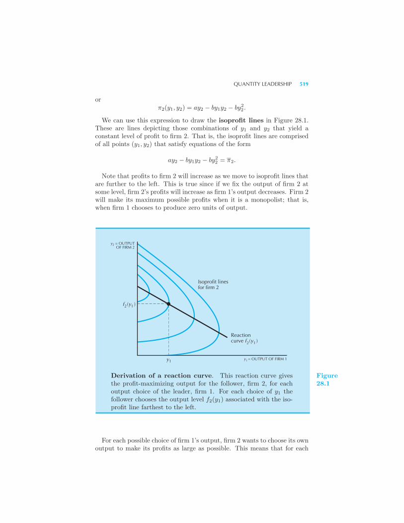
QUANTITY LEADERSHIP 519
orπ2(y1, y2) = ay2 − by1y2 − by22 .
We can use this expression to draw the isoprofit lines in Figure 28.1.These are lines depicting those combinations of y1 and y2 that yield aconstant level of profit to firm 2. That is, the isoprofit lines are comprisedof all points (y1, y2) that satisfy equations of the form
ay2 − by1y2 − by22 = π2.
Note that profits to firm 2 will increase as we move to isoprofit lines thatare further to the left. This is true since if we fix the output of firm 2 atsome level, firm 2’s profits will increase as firm 1’s output decreases. Firm 2will make its maximum possible profits when it is a monopolist; that is,when firm 1 chooses to produce zero units of output.
Reactioncurve f (y )
y = OUTPUT OF FIRM 11
2 1
y1
12f (y )
y2 = OUTPUTOF FIRM 2
Isoprofit linesfor firm 2
Derivation of a reaction curve. This reaction curve givesthe profit-maximizing output for the follower, firm 2, for eachoutput choice of the leader, firm 1. For each choice of y1 thefollower chooses the output level f2(y1) associated with the iso-profit line farthest to the left.
Figure28.1
For each possible choice of firm 1’s output, firm 2 wants to choose its ownoutput to make its profits as large as possible. This means that for each
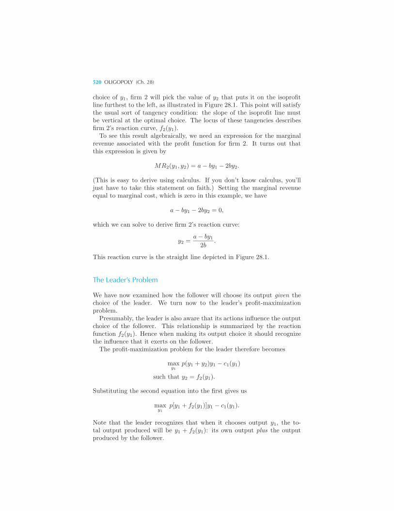
520 OLIGOPOLY (Ch. 28)
choice of y1, firm 2 will pick the value of y2 that puts it on the isoprofitline furthest to the left, as illustrated in Figure 28.1. This point will satisfythe usual sort of tangency condition: the slope of the isoprofit line mustbe vertical at the optimal choice. The locus of these tangencies describesfirm 2’s reaction curve, f2(y1).To see this result algebraically, we need an expression for the marginal
revenue associated with the profit function for firm 2. It turns out thatthis expression is given by
MR2(y1, y2) = a− by1 − 2by2.
(This is easy to derive using calculus. If you don’t know calculus, you’lljust have to take this statement on faith.) Setting the marginal revenueequal to marginal cost, which is zero in this example, we have
a− by1 − 2by2 = 0,
which we can solve to derive firm 2’s reaction curve:
y2 =a− by1
2b.
This reaction curve is the straight line depicted in Figure 28.1.
The Leader’s Problem
We have now examined how the follower will choose its output given thechoice of the leader. We turn now to the leader’s profit-maximizationproblem.Presumably, the leader is also aware that its actions influence the output
choice of the follower. This relationship is summarized by the reactionfunction f2(y1). Hence when making its output choice it should recognizethe influence that it exerts on the follower.The profit-maximization problem for the leader therefore becomes
maxy1
p(y1 + y2)y1 − c1(y1)
such that y2 = f2(y1).
Substituting the second equation into the first gives us
maxy1
p[y1 + f2(y1)]y1 − c1(y1).
Note that the leader recognizes that when it chooses output y1, the to-tal output produced will be y1 + f2(y1): its own output plus the outputproduced by the follower.
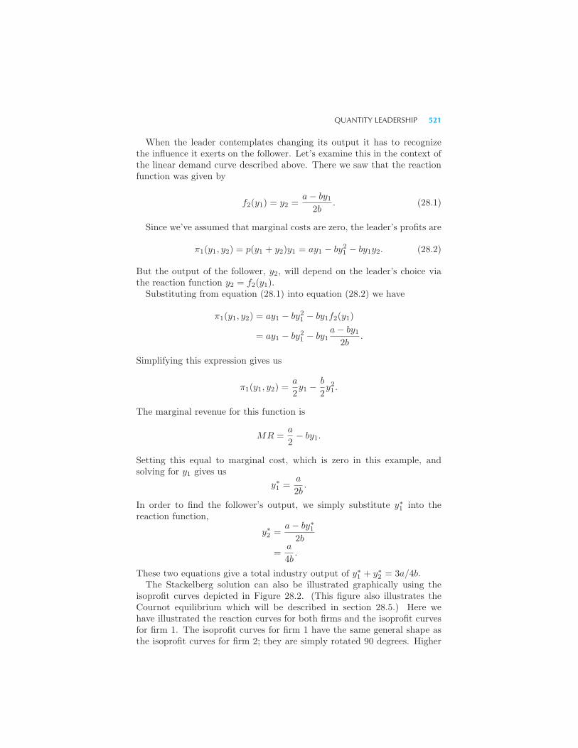
QUANTITY LEADERSHIP 521
When the leader contemplates changing its output it has to recognizethe influence it exerts on the follower. Let’s examine this in the context ofthe linear demand curve described above. There we saw that the reactionfunction was given by
f2(y1) = y2 =a− by1
2b. (28.1)
Since we’ve assumed that marginal costs are zero, the leader’s profits are
π1(y1, y2) = p(y1 + y2)y1 = ay1 − by21 − by1y2. (28.2)
But the output of the follower, y2, will depend on the leader’s choice viathe reaction function y2 = f2(y1).
Substituting from equation (28.1) into equation (28.2) we have
π1(y1, y2) = ay1 − by21 − by1f2(y1)
= ay1 − by21 − by1a− by1
2b.
Simplifying this expression gives us
π1(y1, y2) =a
2y1 −
b
2y21 .
The marginal revenue for this function is
MR =a
2− by1.
Setting this equal to marginal cost, which is zero in this example, andsolving for y1 gives us
y∗1 =a
2b.
In order to find the follower’s output, we simply substitute y∗1 into thereaction function,
y∗2 =a− by∗1
2b
=a
4b.
These two equations give a total industry output of y∗1 + y∗2 = 3a/4b.The Stackelberg solution can also be illustrated graphically using the
isoprofit curves depicted in Figure 28.2. (This figure also illustrates theCournot equilibrium which will be described in section 28.5.) Here wehave illustrated the reaction curves for both firms and the isoprofit curvesfor firm 1. The isoprofit curves for firm 1 have the same general shape asthe isoprofit curves for firm 2; they are simply rotated 90 degrees. Higher
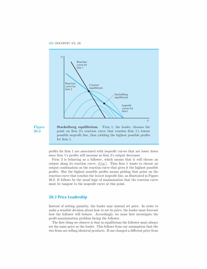
522 OLIGOPOLY (Ch. 28)
Cournotequilibrium
Stackelbergequilibrium
Reactioncurve forfirm 1
Reactioncurve forfirm 2
Isoprofitcurves forfirm1
y1
y2
Figure28.2
Stackelberg equilibrium. Firm 1, the leader, chooses thepoint on firm 2’s reaction curve that touches firm 1’s lowestpossible isoprofit line, thus yielding the highest possible profitsfor firm 1.
profits for firm 1 are associated with isoprofit curves that are lower downsince firm 1’s profits will increase as firm 2’s output decreases.Firm 2 is behaving as a follower, which means that it will choose an
output along its reaction curve, f2(y1). Thus firm 1 wants to choose anoutput combination on the reaction curve that gives it the highest possibleprofits. But the highest possible profits means picking that point on thereaction curve that touches the lowest isoprofit line, as illustrated in Figure28.2. It follows by the usual logic of maximization that the reaction curvemust be tangent to the isoprofit curve at this point.
28.3 Price Leadership
Instead of setting quantity, the leader may instead set price. In order tomake a sensible decision about how to set its price, the leader must forecasthow the follower will behave. Accordingly, we must first investigate theprofit-maximization problem facing the follower.The first thing we observe is that in equilibrium the follower must always
set the same price as the leader. This follows from our assumption that thetwo firms are selling identical products. If one charged a different price from
PRICE LEADERSHIP 523
the other, all of the consumers would prefer the producer with the lowerprice, and we couldn’t have an equilibrium with both firms producing.Suppose that the leader has set a price p. We will suppose that the
follower takes this price as given and chooses its profit-maximizing output.This is essentially the same as the competitive behavior we investigatedearlier. In the competitive model, each firm takes the price as being outsideof its control because it is such a small part of the market; in the price-leadership model, the follower takes the price as being outside of its controlsince it has already been set by the leader.The follower wants to maximize profits:
maxy2
py2 − c2(y2).
This leads to the familiar condition that the follower will want to choosean output level where price equals marginal cost. This determines a supplycurve for the follower, S(p), which we have illustrated in Figure 28.3.
PRICE
Market demand
Follower's supply
Demand curvefacing leader(residual demand)
MR facing leader
MC of leader
QUANTITYy*y*
p*
L r
Price leader. The demand curve facing the leader is themarket demand curve minus the follower’s supply curve. Theleader equates marginal revenue and marginal cost to find theoptimal quantity to supply, y∗L. The total amount supplied tothe market is y∗T and the equilibrium price is p∗.
Figure28.3
Turn now to the problem facing the leader. It realizes that if it setsa price p, the follower will supply S(p). That means that the amount of
524 OLIGOPOLY (Ch. 28)
output the leader will sell will be R(p) = D(p) − S(p). This is called theresidual demand curve facing the leader.Suppose that the leader has a constant marginal cost of production c.
Then the profits that it achieves for any price p are given by:
π1(p) = (p− c)[D(p)− S(p)] = (p− c)R(p).
In order to maximize profits the leader wants to choose a price and outputcombination where marginal revenue equals marginal cost. However, themarginal revenue should be the marginal revenue for the residual demandcurve—the curve that actually measures how much output it will be able tosell at each given price. In Figure 28.3 the residual demand curve is linear;therefore the marginal revenue curve associated with it will have the samevertical intercept and be twice as steep.Let’s look at a simple algebraic example. Suppose that the inverse de-
mand curve isD(p) = a−bp. The follower has a cost function c2(y2) = y22/2,and the leader has a cost function c1(y1) = cy1.For any price p the follower wants to operate where price equals marginal
cost. If the cost function is c2(y2) = y22/2, it can be shown that the marginalcost curve is MC2(y2) = y2. Setting price equal to marginal cost gives us
p = y2.
Solving for the follower’s supply curve gives y2 = S(p) = p.The demand curve facing the leader—the residual demand curve—is
R(p) = D(p)− S(p) = a− bp− p = a− (b+ 1)p.
From now on this is just like an ordinary monopoly problem. Solving forp as a function of the leader’s output y1, we have
p =a
b+ 1− 1
b+ 1y1. (28.3)
This is the inverse demand function facing the leader. The associatedmarginal revenue curve has the same intercept and is twice as steep. Thismeans that it is given by
MR1 =a
b+ 1− 2
b+ 1y1.
Setting marginal revenue equal to marginal cost gives us the equation
MR1 =a
b+ 1− 2
b+ 1y1 = c = MC1.
Solving for the leader’s profit-maximizing output, we have
y∗1 =a− c(b+ 1)
2.
We could go on and substitute this into equation (28.3) to get the equilib-rium price, but the equation is not particularly interesting.

SIMULTANEOUS QUANTITY SETTING 525
28.4 Comparing Price Leadership and Quantity Leadership
We’ve seen how to calculate the equilibrium price and output in the case ofquantity leadership and price leadership. Each model determines a differentequilibrium price and output combination; each model is appropriate indifferent circumstances.One way to think about quantity setting is to think of the firm as making
a capacity choice. When a firm sets a quantity it is in effect determininghow much it is able to supply to the market. If one firm is able to makean investment in capacity first, then it is naturally modeled as a quantityleader.On the other hand, suppose that we look at a market where capacity
choices are not important but one of the firms distributes a catalog ofprices. It is natural to think of this firm as a price setter. Its rivals maythen take the catalog price as given and make their own pricing and supplydecision accordingly.Whether the price-leadership or the quantity-leadership model is appro-
priate is not a question that can be answered on the basis of pure theory.We have to look at how the firms actually make their decisions in order tochoose the most appropriate model.
28.5 Simultaneous Quantity Setting
One difficulty with the leader-follower model is that it is necessarily asym-metric: one firm is able to make its decision before the other firm. In somesituations this is unreasonable. For example, suppose that two firms aresimultaneously trying to decide what quantity to produce. Here each firmhas to forecast what the other firm’s output will be in order to make asensible decision itself.In this section we will examine a one-period model in which each firm
has to forecast the other firm’s output choice. Given its forecast, each firmthen chooses a profit-maximizing output for itself. We then seek an equi-librium in forecasts—a situation where each firm finds its beliefs about theother firm to be confirmed. This model is known as the Cournot model,after the nineteenth-century French mathematician who first examined itsimplications.3
We begin by assuming that firm 1 expects that firm 2 will produce ye2units of output. (The e stands for expected output.) If firm 1 decides toproduce y1 units of output, it expects that the total output produced will
3 Augustin Cournot (pronounced “core-no”) was born in 1801. His book, Researchesinto the Mathematical Principles of the Theory of Wealth, was published in 1838.
526 OLIGOPOLY (Ch. 28)
be Y = y1 + ye2, and output will yield a market price of p(Y ) = p(y1 + ye2).The profit-maximization problem of firm 1 is then
maxy1
p(y1 + ye2)y1 − c(y1).
For any given belief about the output of firm 2, ye2, there will be someoptimal choice of output for firm 1, y1. Let us write this functional rela-tionship between the expected output of firm 2 and the optimal choice offirm 1 as
y1 = f1(ye2).
This function is simply the reaction function that we investigated earlierin this chapter. In our original treatment the reaction function gave thefollower’s output as a function of the leader’s choice. Here the reactionfunction gives one firm’s optimal choice as a function of its beliefs aboutthe other firm’s choice. Although the interpretation of the reaction functionis different in the two cases, the mathematical definition is exactly the same.Similarly, we can derive firm 2’s reaction curve:
y2 = f2(ye1),
which gives firm 2’s optimal choice of output for a given expectation aboutfirm 1’s output, ye1.Now, recall that each firm is choosing its output level assuming that the
other firm’s output will be at ye1 or ye2. For arbitrary values of ye1 and ye2this won’t happen—in general firm 1’s optimal level of output, y1, will bedifferent from what firm 2 expects the output to be, ye1.Let us seek an output combination (y∗1 , y
∗2) such that the optimal output
level for firm 1, assuming firm 2 produces y∗2 , is y∗1 and the optimal output
level for firm 2, assuming that firm 1 stays at y∗1 , is y∗2 . In other words, the
output choices (y∗1 , y∗2) satisfy
y∗1 = f1(y∗2)
y∗2 = f2(y∗1).
Such a combination of output levels is known as a Cournot equilib-rium. In a Cournot equilibrium, each firm is maximizing its profits, givenits beliefs about the other firm’s output choice, and, furthermore, thosebeliefs are confirmed in equilibrium: each firm optimally chooses to pro-duce the amount of output that the other firm expects it to produce. In aCournot equilibrium neither firm will find it profitable to change its outputonce it discovers the choice actually made by the other firm.An example of a Cournot equilibrium is given in Figure 28.2. The
Cournot equilibrium is simply the pair of outputs at which the two reactioncurves cross. At such a point, each firm is producing a profit-maximizinglevel of output given the output choice of the other firm.
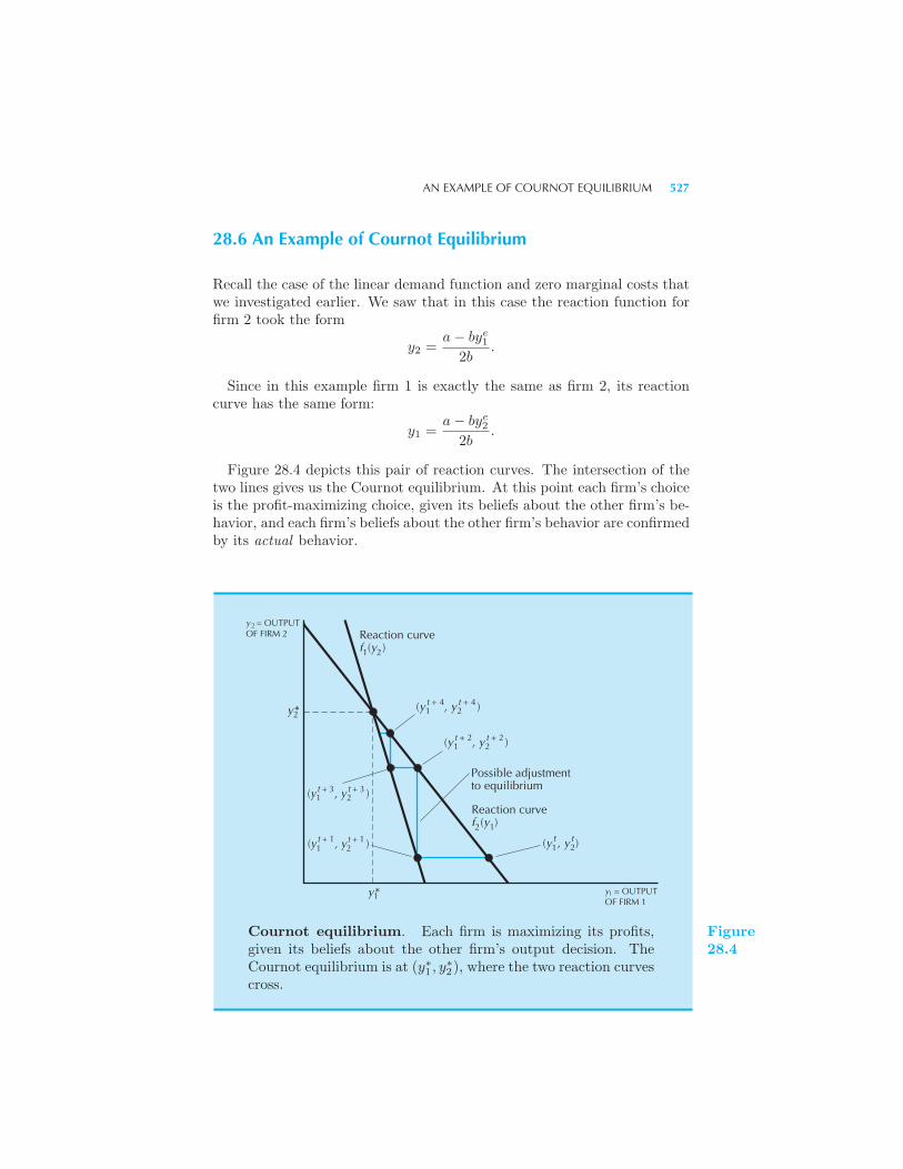
AN EXAMPLE OF COURNOT EQUILIBRIUM 527
28.6 An Example of Cournot Equilibrium
Recall the case of the linear demand function and zero marginal costs thatwe investigated earlier. We saw that in this case the reaction function forfirm 2 took the form
y2 =a− bye1
2b.
Since in this example firm 1 is exactly the same as firm 2, its reactioncurve has the same form:
y1 =a− bye2
2b.
Figure 28.4 depicts this pair of reaction curves. The intersection of thetwo lines gives us the Cournot equilibrium. At this point each firm’s choiceis the profit-maximizing choice, given its beliefs about the other firm’s be-havior, and each firm’s beliefs about the other firm’s behavior are confirmedby its actual behavior.
(y t + 41 , y t + 4
2 )
(y t + 21 , y t + 2
2 )
(y , y )t1 2
t
Possible adjustmentto equilibrium
Reaction curvef (y ) 1 2
Reaction curvef (y ) 12
y = OUTPUTOF FIRM 1
1
y = OUTPUTOF FIRM 2
2
y*
y*1
2
(y t + 31 , y t + 3
2 )
1(y t + 1, y 2t + 1 )
Cournot equilibrium. Each firm is maximizing its profits,given its beliefs about the other firm’s output decision. TheCournot equilibrium is at (y∗1 , y
∗2), where the two reaction curves
cross.
Figure28.4
528 OLIGOPOLY (Ch. 28)
In order to calculate the Cournot equilibrium algebraically, we look forthe point (y1, y2) where each firm is doing what the other firm expects it todo. We set y1 = ye1 and y2 = ye2, which gives us the following two equationsin two unknowns:
y1 =a− by2
2b
y2 =a− by1
2b.
In this example, both firms are identical, so each will produce the samelevel of output in equilibrium. Hence we can substitute y1 = y2 into one ofthe above equations to get
y1 =a− by1
2b.
Solving for y∗1 , we get
y∗1 =a
3b.
Since the two firms are identical, this implies that
y∗2 =a
3b
as well, and the total industry output is
y∗1 + y∗2 =2a
3b.
28.7 Adjustment to Equilibrium
We can use Figure 28.4 to describe a process of adjustment to equilibrium.Suppose that at time t the firms are producing outputs (yt1, y
t2), which are
not necessarily equilibrium outputs. If firm 1 expects that firm 2 is goingto continue to keep its output at yt2, then next period firm 1 would want tochoose the profit-maximizing output given that expectation, namely f1(y
t2).
Thus firm 1’s choice in period t+ 1 will be given by
yt+11 = f1(y
t2).
Firm 2 can reason the same way, so firm 2’s choice next period will be
yt+12 = f2(y
t1).
These equations describe how each firm adjusts its output in the faceof the other firm’s choice. Figure 28.4 illustrates the movement of the
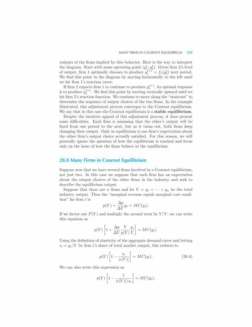
MANY FIRMS IN COURNOT EQUILIBRIUM 529
outputs of the firms implied by this behavior. Here is the way to interpretthe diagram. Start with some operating point (yt1, y
t2). Given firm 2’s level
of output, firm 1 optimally chooses to produce yt+11 = f1(y
t2) next period.
We find this point in the diagram by moving horizontally to the left untilwe hit firm 1’s reaction curve.If firm 2 expects firm 1 to continue to produce yt+1
1 , its optimal responseis to produce yt+1
2 . We find this point by moving vertically upward until wehit firm 2’s reaction function. We continue to move along the “staircase” todetermine the sequence of output choices of the two firms. In the exampleillustrated, this adjustment process converges to the Cournot equilibrium.We say that in this case the Cournot equilibrium is a stable equilibrium.Despite the intuitive appeal of this adjustment process, it does present
some difficulties. Each firm is assuming that the other’s output will befixed from one period to the next, but as it turns out, both firms keepchanging their output. Only in equilibrium is one firm’s expectation aboutthe other firm’s output choice actually satisfied. For this reason, we willgenerally ignore the question of how the equilibrium is reached and focusonly on the issue of how the firms behave in the equilibrium.
28.8 Many Firms in Cournot Equilibrium
Suppose now that we have several firms involved in a Cournot equilibrium,not just two. In this case we suppose that each firm has an expectationabout the output choices of the other firms in the industry and seek todescribe the equilibrium output.Suppose that there are n firms and let Y = y1 + · · · + yn be the total
industry output. Then the “marginal revenue equals marginal cost condi-tion” for firm i is
p(Y ) +Δp
ΔYyi = MC(yi).
If we factor out P (Y ) and multiply the second term by Y/Y , we can writethis equation as
p(Y )
[1 +
Δp
ΔY
Y
p(Y )
yiY
]= MC(yi).
Using the definition of elasticity of the aggregate demand curve and lettingsi = yi/Y be firm i’s share of total market output, this reduces to
p(Y )
[1− si
|ε(Y )|
]= MC(yi). (28.4)
We can also write this expression as
p(Y )
[1− 1
|ε(Y )|/si
]= MC(yi).
530 OLIGOPOLY (Ch. 28)
This looks just like the expression for the monopolist except for the siterm. We can think of |ε(Y )|/si as being the elasticity of the demandcurve facing the firm: the smaller the market share of the firm, the moreelastic the demand curve it faces.If its market share is 1—the firm is a monopolist—the demand curve
facing the firm is the market demand curve, so the condition just reducesto that of the monopolist. If the firm is a very small part of a large market,its market share is effectively zero, and the demand curve facing the firm iseffectively flat. Thus the condition reduces to that of the pure competitor:price equals marginal cost.This is one justification for the competitive model described in Chap-
ter 23. If there are a large number of firms, then each firm’s influence onthe market price is negligible, and the Cournot equilibrium is effectivelythe same as pure competition.
28.9 Simultaneous Price Setting
In the Cournot model described above we have assumed that firms werechoosing their quantities and letting the market determine the price. An-other approach is to think of firms as setting their prices and letting themarket determine the quantity sold. This model is known as Bertrandcompetition.4
When a firm chooses its price, it has to forecast the price set by the otherfirm in the industry. Just as in the case of Cournot equilibrium we wantto find a pair of prices such that each price is a profit-maximizing choicegiven the choice made by the other firm.What does a Bertrand equilibrium look like? When firms are selling
identical products, as we have been assuming, the Bertrand equilibriumhas a very simple structure indeed. It turns out to be the competitiveequilibrium, where price equals marginal cost!First we note that price can never be less than marginal cost since then
either firm would increase its profits by producing less. So let us considerthe case where price is greater than marginal cost. Suppose that both firmsare selling output at some price p greater than marginal cost. Consider theposition of firm 1. If it lowers its price by any small amount ε and if theother firm keeps its price fixed at p, all of the consumers will prefer topurchase from firm 1. By cutting its price by an arbitrarily small amount,it can steal all of the customers from firm 2.If firm 1 really believes that firm 2 will charge a price p that is greater
than marginal cost, it will always pay firm 1 to cut its price to p− ε. Butfirm 2 can reason the same way! Thus any price higher than marginal
4 Joseph Bertrand, also a French mathematician, presented his model in a review ofCournot’s work.
COLLUSION 531
cost cannot be an equilibrium; the only equilibrium is the competitiveequilibrium.This result seems paradoxical when you first encounter it: how can we
get a competitive price if there are only two firms in the market? If wethink of the Bertrand model as a model of competitive bidding it makesmore sense. Suppose that one firm “bids” for the consumers’ business byquoting a price above marginal cost. Then the other firm can always makea profit by undercutting this price with a lower price. It follows that theonly price that each firm cannot rationally expect to be undercut is a priceequal to marginal cost.It is often observed that competitive bidding among firms that are unable
to collude can result in prices that are much lower than can be achievedby other means. This phenomenon is simply an example of the logic ofBertrand competition.
28.10 Collusion
In the models we have examined up until now the firms have operatedindependently. But if the firms collude so as to jointly determine theiroutput, these models are not very reasonable. If collusion is possible, thefirms would do better to choose the output that maximizes total industryprofits and then divide up the profits among themselves. When firms gettogether and attempt to set prices and outputs so as to maximize totalindustry profits, they are known as a cartel. As we saw in Chapter 25, acartel is simply a group of firms that jointly collude to behave like a singlemonopolist and maximize the sum of their profits.Thus the profit-maximization problem facing the two firms is to choose
their outputs y1 and y2 so as to maximize total industry profits:
maxy1,y2
p(y1 + y2)[y1 + y2]− c1(y1)− c2(y2).
This will have the optimality conditions
p(y∗1 + y∗2) +Δp
ΔY[y∗1 + y∗2 ] = MC1(y
∗1)
p(y∗1 + y∗2) +Δp
ΔY[y∗1 + y∗2 ] = MC2(y
∗2).
The interpretation of these conditions is interesting. When firm 1 consid-ers expanding its output by Δy1, it will contemplate the usual two effects:the extra profits from selling more output and the reduction in profits fromforcing the price down. But in the second effect, it now takes into accountthe effect of the lower price on both its own output and the output of the
532 OLIGOPOLY (Ch. 28)
other firm. This is because it is now interested in maximizing total industryprofits, not just its own profits.The optimality conditions imply that the marginal revenue of an extra
unit of output must be the same no matter where it is produced. It followsthat MC1(y
∗1) = MC2(y
∗2), so that the two marginal costs will be equal in
equilibrium. If one firm has a cost advantage, so that its marginal cost curvealways lies below that of the other firm, then it will necessarily producemore output in equilibrium in the cartel solution.The problem with agreeing to join a cartel in real life is that there is
always a temptation to cheat. Suppose, for example, that the two firmsare operating at the outputs that maximize industry profits (y∗1 , y
∗2) and
firm 1 considers producing a little more output, Δy1. The marginal profitsaccruing to firm 1 will be
Δπ1
Δy1= p(y∗1 + y∗2) +
Δp
ΔYy∗1 −MC1(y
∗1). (28.5)
We saw earlier that the optimality condition for the cartel solution is
p(y∗1 + y∗2) +Δp
ΔYy∗1 +
Δp
ΔYy∗2 −MC1(y
∗1) = 0.
Rearranging this equation gives us
p(y∗1 + y∗2) +Δp
ΔYy∗1 −MC1(y
∗1) = − Δp
ΔYy∗2 > 0. (28.6)
The last inequality follows since Δp/ΔY is negative, since the market de-mand curve has a negative slope.Inspecting equations (28.5) and (28.6) we see that
Δπ1
Δy1> 0.
Thus, if firm 1 believes that firm 2 will keep its output fixed, then it willbelieve that it can increase profits by increasing its own production. In thecartel solution, the firms act together to restrict output so as not to “spoil”the market. They recognize the effect on joint profits from producing moreoutput in either firm. But if each firm believes that the other firm willstick to its output quota, then each firm will be tempted to increase itsown profits by unilaterally expanding its output. At the output levelsthat maximize joint profits, it will always be profitable for each firm tounilaterally increase its output—if each firm expects that the other firmwill keep its output fixed.The situation is even worse than that. If firm 1 believes that firm 2
will keep its output fixed, then it will find it profitable to increase itsown output. But if it thinks that firm 2 will increase its output, then
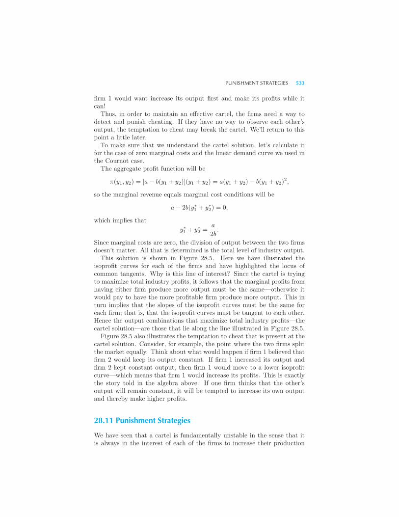
PUNISHMENT STRATEGIES 533
firm 1 would want increase its output first and make its profits while itcan!Thus, in order to maintain an effective cartel, the firms need a way to
detect and punish cheating. If they have no way to observe each other’soutput, the temptation to cheat may break the cartel. We’ll return to thispoint a little later.To make sure that we understand the cartel solution, let’s calculate it
for the case of zero marginal costs and the linear demand curve we used inthe Cournot case.The aggregate profit function will be
π(y1, y2) = [a− b(y1 + y2)](y1 + y2) = a(y1 + y2)− b(y1 + y2)2,
so the marginal revenue equals marginal cost conditions will be
a− 2b(y∗1 + y∗2) = 0,
which implies that
y∗1 + y∗2 =a
2b.
Since marginal costs are zero, the division of output between the two firmsdoesn’t matter. All that is determined is the total level of industry output.This solution is shown in Figure 28.5. Here we have illustrated the
isoprofit curves for each of the firms and have highlighted the locus ofcommon tangents. Why is this line of interest? Since the cartel is tryingto maximize total industry profits, it follows that the marginal profits fromhaving either firm produce more output must be the same—otherwise itwould pay to have the more profitable firm produce more output. This inturn implies that the slopes of the isoprofit curves must be the same foreach firm; that is, that the isoprofit curves must be tangent to each other.Hence the output combinations that maximize total industry profits—thecartel solution—are those that lie along the line illustrated in Figure 28.5.Figure 28.5 also illustrates the temptation to cheat that is present at the
cartel solution. Consider, for example, the point where the two firms splitthe market equally. Think about what would happen if firm 1 believed thatfirm 2 would keep its output constant. If firm 1 increased its output andfirm 2 kept constant output, then firm 1 would move to a lower isoprofitcurve—which means that firm 1 would increase its profits. This is exactlythe story told in the algebra above. If one firm thinks that the other’soutput will remain constant, it will be tempted to increase its own outputand thereby make higher profits.
28.11 Punishment Strategies
We have seen that a cartel is fundamentally unstable in the sense that itis always in the interest of each of the firms to increase their production
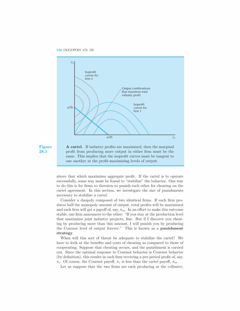
534 OLIGOPOLY (Ch. 28)
y2
Isoprofitcurves forfirm 2
Isoprofitcurves forfirm 1
Output combinationsthat maximize totalindustry profit
y1
a/2b
a/2b
Figure28.5
A cartel. If industry profits are maximized, then the marginalprofit from producing more output in either firm must be thesame. This implies that the isoprofit curves must be tangent toone another at the profit-maximizing levels of output.
above that which maximizes aggregate profit. If the cartel is to operatesuccessfully, some way must be found to “stabilize” the behavior. One wayto do this is for firms to threaten to punish each other for cheating on thecartel agreement. In this section, we investigate the size of punishmentsnecessary to stabilize a cartel.
Consider a duopoly composed of two identical firms. If each firm pro-duces half the monopoly amount of output, total profits will be maximizedand each firm will get a payoff of, say, πm. In an effort to make this outcomestable, one firm announces to the other: “If you stay at the production levelthat maximizes joint industry projects, fine. But if I discover you cheat-ing by producing more than this amount, I will punish you by producingthe Cournot level of output forever.” This is known as a punishmentstrategy.
When will this sort of threat be adequate to stabilize the cartel? Wehave to look at the benefits and costs of cheating as compared to those ofcooperating. Suppose that cheating occurs, and the punishment is carriedout. Since the optimal response to Cournot behavior is Cournot behavior(by definition), this results in each firm receiving a per-period profit of, say,πc. Of course, the Cournot payoff, πc is less than the cartel payoff, πm.
Let us suppose that the two firms are each producing at the collusive,
PUNISHMENT STRATEGIES 535
monopoly level of production. Put yourself in the place of one of thefirms trying to decide whether to continue to produce at your quota. Ifyou produce more output, deviating from your quota, you make profit πd,where πd > πm. This is the standard temptation facing a cartel memberdescribed above: if each firm restricts output and pushes the price up, theneach firm has an incentive to capitalize on the high price by increasing itsproduction.But this isn’t the end of the story because of the punishment for cheating.
By producing at the cartel amount, each firm gets a steady stream ofpayments of πm. The present value of this stream starting today is givenby
Present value of cartel behavior = πm +πm
r.
If the firm produces more than the cartel amount, it gets a one-time benefitof profits πd, but then has to live with the breakup of the cartel and thereversion to Cournot behavior:
Present value of cheating = πd +πc
r.
When will the present value of remaining at the cartel output be greaterthan the present value of cheating on the cartel agreement? Obviouslywhen
πm +πm
r> πd +
πc
r,
which can also be written as
r <πm − πc
πd − πm.
Note that the numerator of this fraction is positive, since the monopolyprofits are larger than the Cournot profits, and the denominator is positive,since deviation is even more profitable than sticking with the monopolyquota.The inequality says that as long as the interest rate is sufficiently small,
so that the prospect of future punishment is sufficiently important, it willpay the firms to stick to their quotas.The weakness of this model is that the threat to revert to Cournot be-
havior forever is not very believable. One firm certainly may believe thatthe other will punish it for deviating, but “forever” is a long time. A morerealistic model would consider shorter periods of retaliation, but the analy-sis then becomes much more complex. In the next chapter, we discuss somemodels of “repeated games” that illustrate some of the possible behaviors.
EXAMPLE: Price Matching and Competition
We have seen that there is always a temptation for each member of acartel to produce more than its quota. In order to maintain a successful

536 OLIGOPOLY (Ch. 28)
cartel, some way must be found to police members’ behavior by some formof punishment for deviations from the joint profit-maximizing output. Inparticular this means that firms must be able to keep track of the pricesand production levels of the other firms in the cartel.One easy way to acquire information about what the other firms in your
industry are charging is to use your customers to spy on the other firms.It is common to see retail firms announce that they will “beat any price.”In some cases, such an offer may indicate a highly competitive retail en-vironment. But in other cases, this same policy can be used to gatherinformation about other firms’ prices in order to maintain a cartel.Suppose, for example, that two firms agree, either explicitly or implicitly
to sell a certain model of refrigerator for $700. How can either of the storesbe sure that the other firm isn’t cheating on their agreement and sellingthe refrigerator for $675? One way is to offer to beat any price a customercan find. That way, the customers report any attempts to cheat on thecollusive arrangement.
EXAMPLE: Voluntary Export Restraints
During the 1980s, the Japanese automobile companies agreed to a “volun-tary export restraint (VER).” This meant that they would “voluntarily”reduce the exports of their automobiles to the United States. The typ-ical U.S. consumer thought that this was a great victory for U.S. tradenegotiators.But if you think about this for a minute, things look quite different. In
our examination of oligopoly we have seen that the problem facing firms inan industry is how to restrict output in order to support higher prices anddiscourage competition. As we’ve seen, there will always be a temptationto cheat on production agreements; every cartel must find a way to detectand prevent this cheating. It is especially convenient for the firms if a thirdparty, such as the government, can serve this role. This is exactly the rolethat the U.S. government played for the Japanese auto makers!According to one estimate Japanese imported cars were about $2500
more expensive in 1984 than they would have been without the VERs.Furthermore, the higher prices of imported cars allowed American produc-ers to sell their automobiles at about $1000 more than they would haveotherwise.5
Due to these higher prices the U.S. consumers paid about $10 billionmore for Japanese cars in 1985–86 than they would have otherwise. Thismoney has gone directly into the pockets of the Japanese automobile pro-ducers. Much of this additional profit appears to have been invested in
5 Robert Crandall, “Import Quotas and the Automobile Industry: the Costs of Pro-tectionism,” The Brookings Review, Summer, 1984.
SUMMARY 537
increasing productive capabilities, which allowed the Japanese auto pro-ducers to reduce the cost of producing new cars in subsequent years. TheVERs did succeed in saving American jobs; however, it appears that thecost per job saved was about $160,000 per year.If the goal of the VER policy was simply to increase the health of the
American automobile industry, there was a much simpler way to do this:just impose a $2500 tariff on each imported Japanese car. This way therevenues due to the restriction of trade would accrue to the U.S. governmentrather than to the Japanese automobile industry. Rather than send $10billion abroad during 1985–86, the U.S. government could have spent themoney on projects designed to increase the long-term health of the U.S.auto industry.
28.12 Comparison of the Solutions
We have now examined several models of duopoly behavior: quantityleadership (Stackelberg), price leadership, simultaneous quantity setting(Cournot), simultaneous price setting (Bertrand), and the collusive solu-tion. How do they compare?In general, collusion results in the smallest industry output and the high-
est price. Bertrand equilibrium—the competitive equilibrium—gives us thehighest output and the lowest price. The other models give results that arein between these two extremes.A variety of other models are possible. For example, we could look at a
model with differentiated products where the two goods produced were notperfect substitutes for each other. Or we could look at a model where thefirms make a sequence of choices over time. In this framework, the choicesthat one firm makes at one time can influence the choices that the otherfirm makes later on.We have also assumed that each firm knows the demand function and the
cost functions of the other firms in the industry. In reality these functionsare never known for sure. Each firm needs to estimate the demand andcost conditions facing its rivals when it makes its own decisions. All ofthese phenomena have been modeled by economists, but the models becomemuch more complex.
Summary
1. An oligopoly is characterized by a market with a few firms that rec-ognize their strategic interdependence. There are several possible waysfor oligopolies to behave depending on the exact nature of their interac-tion.
538 OLIGOPOLY (Ch. 28)
2. In the quantity-leader (Stackelberg) model one firm leads by setting itsoutput, and the other firm follows. When the leader chooses an output, itwill take into account how the follower will respond.
3. In the price-leader model, one firm sets its price, and the other firmchooses how much it wants to supply at that price. Again the leader hasto take into account the behavior of the follower when it makes its deci-sion.
4. In the Cournot model, each firm chooses its output so as to maximizeits profits given its beliefs about the other firm’s choice. In equilibriumeach firm finds that its expectation about the other firm’s choice is con-firmed.
5. A Cournot equilibrium in which each firm has a small market shareimplies that price will be very close to marginal cost—that is, the industrywill be nearly competitive.
6. In the Bertrand model each firm chooses its price given its beliefs aboutthe price that the other firm will choose. The only equilibrium price is thecompetitive equilibrium.
7. A cartel consists of a number of firms colluding to restrict output and tomaximize industry profit. A cartel will typically be unstable in the sensethat each firm will be tempted to sell more than its agreed upon output ifit believes that the other firms will not respond.
REVIEW QUESTIONS
1. Suppose that we have two firms that face a linear demand curve p(Y ) =a − bY and have constant marginal costs, c, for each firm. Solve for theCournot equilibrium output.
2. Consider a cartel in which each firm has identical and constant marginalcosts. If the cartel maximizes total industry profits, what does this implyabout the division of output between the firms?
3. Can the leader ever get a lower profit in a Stackelberg equilibrium thanhe would get in the Cournot equilibrium?
4. Suppose there are n identical firms in a Cournot equilibrium. Show thatthe absolute value of the elasticity of the market demand curve must begreater than 1/n. (Hint: in the case of a monopolist, n = 1, and thissimply says that a monopolist operates at an elastic part of the demandcurve. Apply the logic that we used to establish that fact to this problem.)

REVIEW QUESTIONS 539
5. Draw a set of reaction curves that result in an unstable equilibrium.
6. Do oligopolies produce an efficient level of output?
CHAPTER 29
GAMETHEORY
The previous chapter on oligopoly theory presented the classical economictheory of strategic interaction among firms. But that is really just the tipof the iceberg. Economic agents can interact strategically in a variety ofways, and many of these have been studied by using the apparatus of gametheory. Game theory is concerned with the general analysis of strategicinteraction. It can be used to study parlor games, political negotiation, andeconomic behavior. In this chapter we will briefly explore this fascinatingsubject to give you a flavor of how it works and how it can be used to studyeconomic behavior in oligopolistic markets.
29.1 The Payoff Matrix of a Game
Strategic interaction can involve many players and many strategies, butwe’ll limit ourselves to two-person games with a finite number of strategies.This will allow us to depict the game easily in a payoff matrix. It issimplest to examine this in the context of a specific example.Suppose that two people are playing a simple game. Person A will write
one of two words on a piece of paper, “top” or “bottom.” Simultaneously,
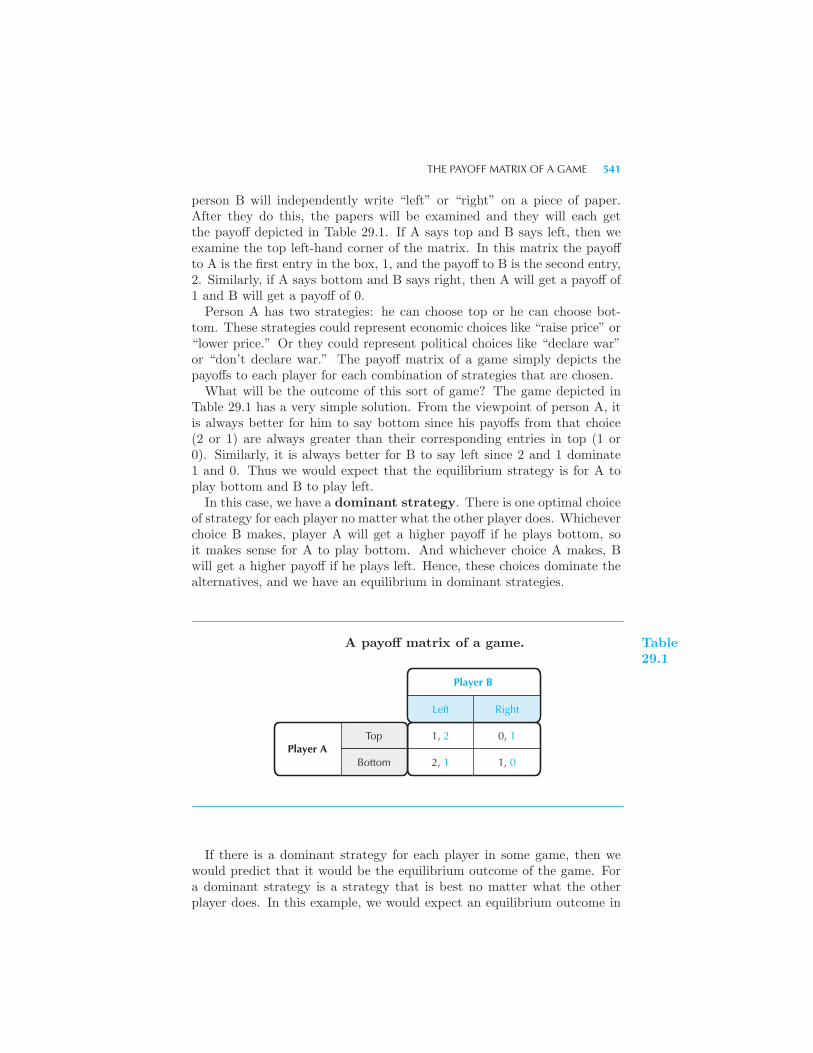
THE PAYOFF MATRIX OF A GAME 541
person B will independently write “left” or “right” on a piece of paper.After they do this, the papers will be examined and they will each getthe payoff depicted in Table 29.1. If A says top and B says left, then weexamine the top left-hand corner of the matrix. In this matrix the payoffto A is the first entry in the box, 1, and the payoff to B is the second entry,2. Similarly, if A says bottom and B says right, then A will get a payoff of1 and B will get a payoff of 0.Person A has two strategies: he can choose top or he can choose bot-
tom. These strategies could represent economic choices like “raise price” or“lower price.” Or they could represent political choices like “declare war”or “don’t declare war.” The payoff matrix of a game simply depicts thepayoffs to each player for each combination of strategies that are chosen.What will be the outcome of this sort of game? The game depicted in
Table 29.1 has a very simple solution. From the viewpoint of person A, itis always better for him to say bottom since his payoffs from that choice(2 or 1) are always greater than their corresponding entries in top (1 or0). Similarly, it is always better for B to say left since 2 and 1 dominate1 and 0. Thus we would expect that the equilibrium strategy is for A toplay bottom and B to play left.In this case, we have a dominant strategy. There is one optimal choice
of strategy for each player no matter what the other player does. Whicheverchoice B makes, player A will get a higher payoff if he plays bottom, soit makes sense for A to play bottom. And whichever choice A makes, Bwill get a higher payoff if he plays left. Hence, these choices dominate thealternatives, and we have an equilibrium in dominant strategies.
Player B
Player ATop
Bottom
1, 2
2, 1
0, 1
1, 0
Left Right
A payoff matrix of a game. Table29.1
If there is a dominant strategy for each player in some game, then wewould predict that it would be the equilibrium outcome of the game. Fora dominant strategy is a strategy that is best no matter what the otherplayer does. In this example, we would expect an equilibrium outcome in
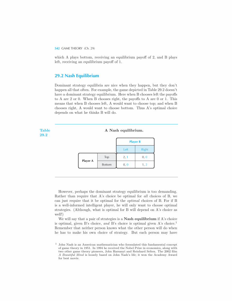
542 GAME THEORY (Ch. 29)
which A plays bottom, receiving an equilibrium payoff of 2, and B playsleft, receiving an equilibrium payoff of 1.
29.2 Nash Equilibrium
Dominant strategy equilibria are nice when they happen, but they don’thappen all that often. For example, the game depicted in Table 29.2 doesn’thave a dominant strategy equilibrium. Here when B chooses left the payoffsto A are 2 or 0. When B chooses right, the payoffs to A are 0 or 1. Thismeans that when B chooses left, A would want to choose top; and when Bchooses right, A would want to choose bottom. Thus A’s optimal choicedepends on what he thinks B will do.
Player B
Player ATop
Bottom
2, 1
0, 0
0, 0
1, 2
Left Right
Table29.2
A Nash equilibrium.
However, perhaps the dominant strategy equilibrium is too demanding.Rather than require that A’s choice be optimal for all choices of B, wecan just require that it be optimal for the optimal choices of B. For if Bis a well-informed intelligent player, he will only want to choose optimalstrategies. (Although, what is optimal for B will depend on A’s choice aswell!)We will say that a pair of strategies is a Nash equilibrium if A’s choice
is optimal, given B’s choice, and B’s choice is optimal given A’s choice.1
Remember that neither person knows what the other person will do whenhe has to make his own choice of strategy. But each person may have
1 John Nash is an American mathematician who formulated this fundamental conceptof game theory in 1951. In 1994 he received the Nobel Prize in economics, along withtwo other game theory pioneers, John Harsanyi and Reinhard Selten. The 2002 filmA Beautiful Mind is loosely based on John Nash’s life; it won the Academy Awardfor best movie.
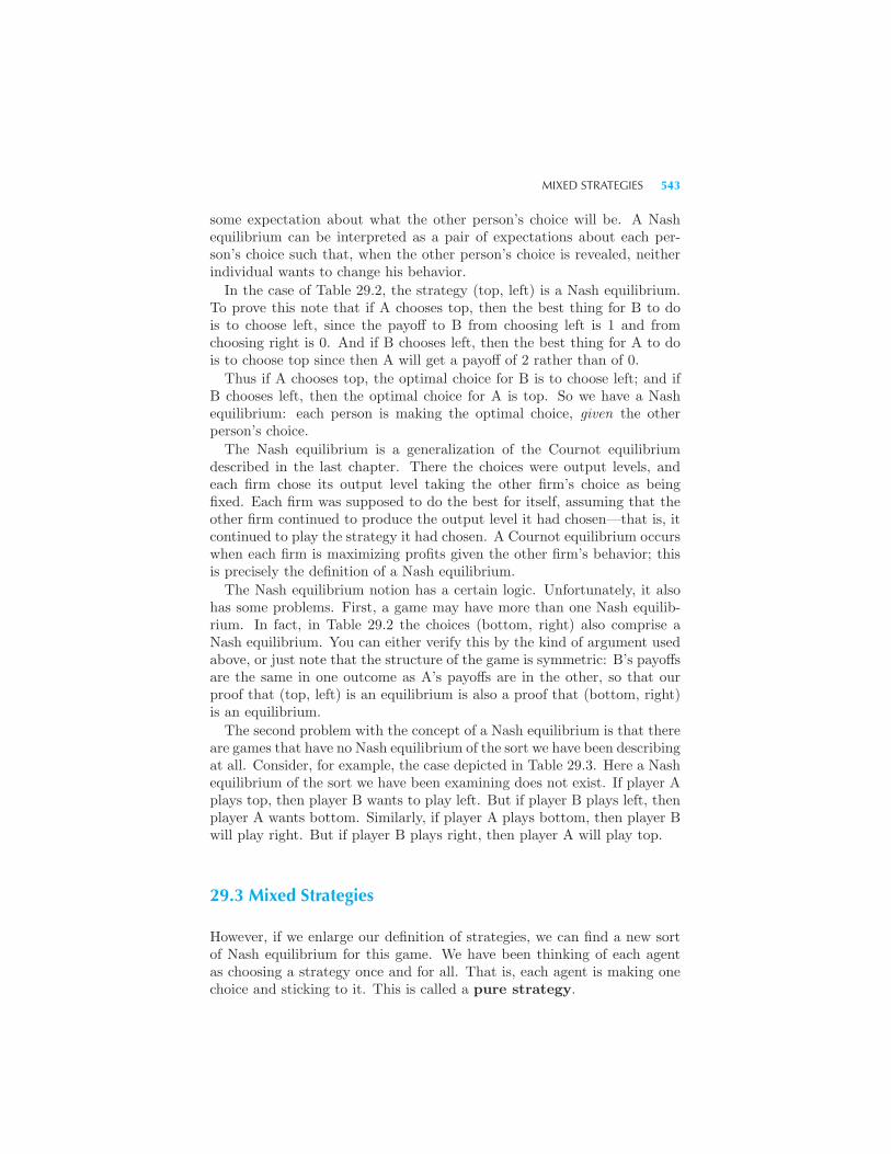
MIXED STRATEGIES 543
some expectation about what the other person’s choice will be. A Nashequilibrium can be interpreted as a pair of expectations about each per-son’s choice such that, when the other person’s choice is revealed, neitherindividual wants to change his behavior.
In the case of Table 29.2, the strategy (top, left) is a Nash equilibrium.To prove this note that if A chooses top, then the best thing for B to dois to choose left, since the payoff to B from choosing left is 1 and fromchoosing right is 0. And if B chooses left, then the best thing for A to dois to choose top since then A will get a payoff of 2 rather than of 0.
Thus if A chooses top, the optimal choice for B is to choose left; and ifB chooses left, then the optimal choice for A is top. So we have a Nashequilibrium: each person is making the optimal choice, given the otherperson’s choice.
The Nash equilibrium is a generalization of the Cournot equilibriumdescribed in the last chapter. There the choices were output levels, andeach firm chose its output level taking the other firm’s choice as beingfixed. Each firm was supposed to do the best for itself, assuming that theother firm continued to produce the output level it had chosen—that is, itcontinued to play the strategy it had chosen. A Cournot equilibrium occurswhen each firm is maximizing profits given the other firm’s behavior; thisis precisely the definition of a Nash equilibrium.
The Nash equilibrium notion has a certain logic. Unfortunately, it alsohas some problems. First, a game may have more than one Nash equilib-rium. In fact, in Table 29.2 the choices (bottom, right) also comprise aNash equilibrium. You can either verify this by the kind of argument usedabove, or just note that the structure of the game is symmetric: B’s payoffsare the same in one outcome as A’s payoffs are in the other, so that ourproof that (top, left) is an equilibrium is also a proof that (bottom, right)is an equilibrium.
The second problem with the concept of a Nash equilibrium is that thereare games that have no Nash equilibrium of the sort we have been describingat all. Consider, for example, the case depicted in Table 29.3. Here a Nashequilibrium of the sort we have been examining does not exist. If player Aplays top, then player B wants to play left. But if player B plays left, thenplayer A wants bottom. Similarly, if player A plays bottom, then player Bwill play right. But if player B plays right, then player A will play top.
29.3 Mixed Strategies
However, if we enlarge our definition of strategies, we can find a new sortof Nash equilibrium for this game. We have been thinking of each agentas choosing a strategy once and for all. That is, each agent is making onechoice and sticking to it. This is called a pure strategy.
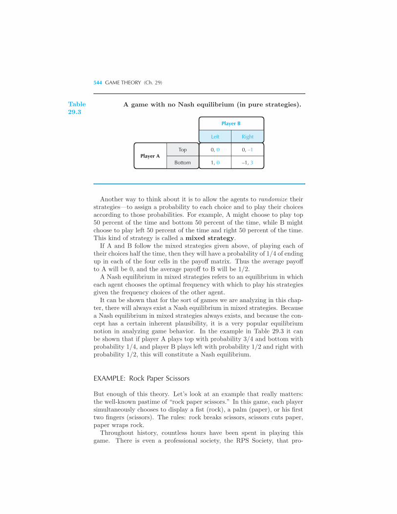
544 GAME THEORY (Ch. 29)
Player B
Player ATop
Bottom
0, 0
1, 0
0, –1
–1, 3
Left Right
Table29.3
A game with no Nash equilibrium (in pure strategies).
Another way to think about it is to allow the agents to randomize theirstrategies—to assign a probability to each choice and to play their choicesaccording to those probabilities. For example, A might choose to play top50 percent of the time and bottom 50 percent of the time, while B mightchoose to play left 50 percent of the time and right 50 percent of the time.This kind of strategy is called a mixed strategy.
If A and B follow the mixed strategies given above, of playing each oftheir choices half the time, then they will have a probability of 1/4 of endingup in each of the four cells in the payoff matrix. Thus the average payoffto A will be 0, and the average payoff to B will be 1/2.A Nash equilibrium in mixed strategies refers to an equilibrium in which
each agent chooses the optimal frequency with which to play his strategiesgiven the frequency choices of the other agent.It can be shown that for the sort of games we are analyzing in this chap-
ter, there will always exist a Nash equilibrium in mixed strategies. Becausea Nash equilibrium in mixed strategies always exists, and because the con-cept has a certain inherent plausibility, it is a very popular equilibriumnotion in analyzing game behavior. In the example in Table 29.3 it canbe shown that if player A plays top with probability 3/4 and bottom withprobability 1/4, and player B plays left with probability 1/2 and right withprobability 1/2, this will constitute a Nash equilibrium.
EXAMPLE: Rock Paper Scissors
But enough of this theory. Let’s look at an example that really matters:the well-known pastime of “rock paper scissors.” In this game, each playersimultaneously chooses to display a fist (rock), a palm (paper), or his firsttwo fingers (scissors). The rules: rock breaks scissors, scissors cuts paper,paper wraps rock.Throughout history, countless hours have been spent in playing this
game. There is even a professional society, the RPS Society, that pro-
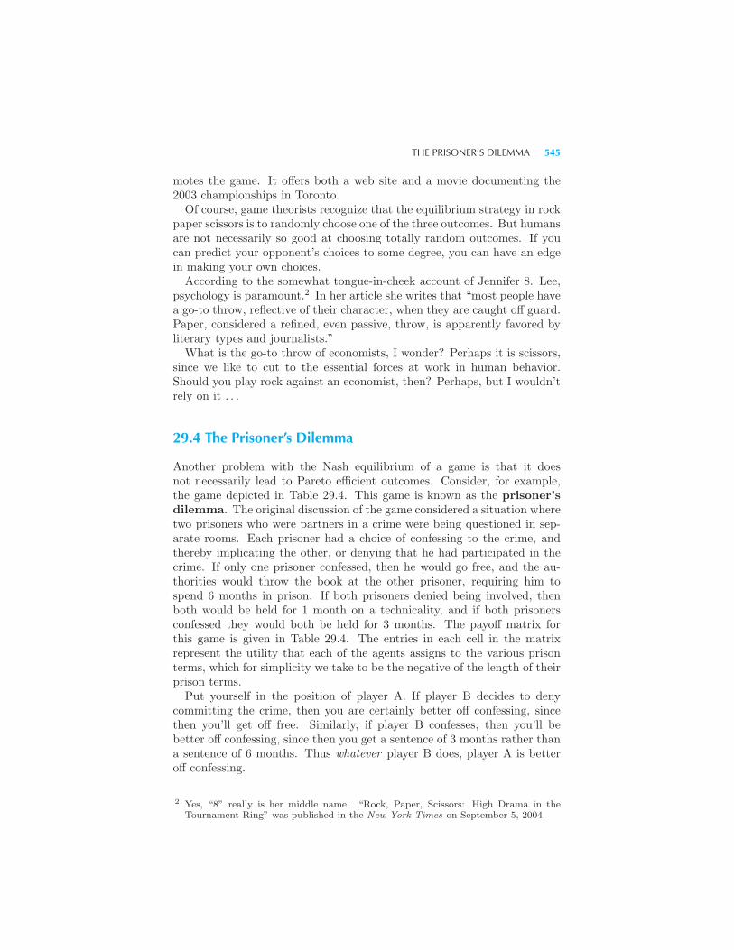
THE PRISONER’S DILEMMA 545
motes the game. It offers both a web site and a movie documenting the2003 championships in Toronto.Of course, game theorists recognize that the equilibrium strategy in rock
paper scissors is to randomly choose one of the three outcomes. But humansare not necessarily so good at choosing totally random outcomes. If youcan predict your opponent’s choices to some degree, you can have an edgein making your own choices.According to the somewhat tongue-in-cheek account of Jennifer 8. Lee,
psychology is paramount.2 In her article she writes that “most people havea go-to throw, reflective of their character, when they are caught off guard.Paper, considered a refined, even passive, throw, is apparently favored byliterary types and journalists.”What is the go-to throw of economists, I wonder? Perhaps it is scissors,
since we like to cut to the essential forces at work in human behavior.Should you play rock against an economist, then? Perhaps, but I wouldn’trely on it . . .
29.4 The Prisoner’s Dilemma
Another problem with the Nash equilibrium of a game is that it doesnot necessarily lead to Pareto efficient outcomes. Consider, for example,the game depicted in Table 29.4. This game is known as the prisoner’sdilemma. The original discussion of the game considered a situation wheretwo prisoners who were partners in a crime were being questioned in sep-arate rooms. Each prisoner had a choice of confessing to the crime, andthereby implicating the other, or denying that he had participated in thecrime. If only one prisoner confessed, then he would go free, and the au-thorities would throw the book at the other prisoner, requiring him tospend 6 months in prison. If both prisoners denied being involved, thenboth would be held for 1 month on a technicality, and if both prisonersconfessed they would both be held for 3 months. The payoff matrix forthis game is given in Table 29.4. The entries in each cell in the matrixrepresent the utility that each of the agents assigns to the various prisonterms, which for simplicity we take to be the negative of the length of theirprison terms.Put yourself in the position of player A. If player B decides to deny
committing the crime, then you are certainly better off confessing, sincethen you’ll get off free. Similarly, if player B confesses, then you’ll bebetter off confessing, since then you get a sentence of 3 months rather thana sentence of 6 months. Thus whatever player B does, player A is betteroff confessing.
2 Yes, “8” really is her middle name. “Rock, Paper, Scissors: High Drama in theTournament Ring” was published in the New York Times on September 5, 2004.
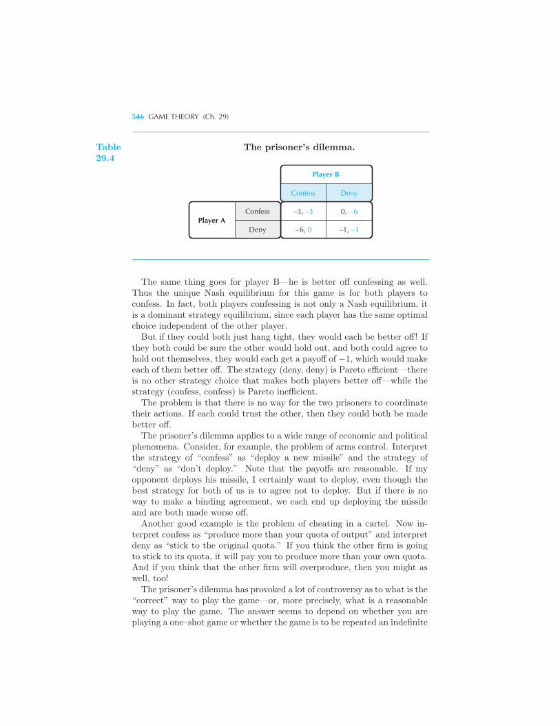
546 GAME THEORY (Ch. 29)
Player B
Player AConfess
Deny
–3, –3
–6, 0
0, –6
–1, –1
Confess Deny
Table29.4
The prisoner’s dilemma.
The same thing goes for player B—he is better off confessing as well.Thus the unique Nash equilibrium for this game is for both players toconfess. In fact, both players confessing is not only a Nash equilibrium, itis a dominant strategy equilibrium, since each player has the same optimalchoice independent of the other player.But if they could both just hang tight, they would each be better off! If
they both could be sure the other would hold out, and both could agree tohold out themselves, they would each get a payoff of −1, which would makeeach of them better off. The strategy (deny, deny) is Pareto efficient—thereis no other strategy choice that makes both players better off—while thestrategy (confess, confess) is Pareto inefficient.The problem is that there is no way for the two prisoners to coordinate
their actions. If each could trust the other, then they could both be madebetter off.The prisoner’s dilemma applies to a wide range of economic and political
phenomena. Consider, for example, the problem of arms control. Interpretthe strategy of “confess” as “deploy a new missile” and the strategy of“deny” as “don’t deploy.” Note that the payoffs are reasonable. If myopponent deploys his missile, I certainly want to deploy, even though thebest strategy for both of us is to agree not to deploy. But if there is noway to make a binding agreement, we each end up deploying the missileand are both made worse off.Another good example is the problem of cheating in a cartel. Now in-
terpret confess as “produce more than your quota of output” and interpretdeny as “stick to the original quota.” If you think the other firm is goingto stick to its quota, it will pay you to produce more than your own quota.And if you think that the other firm will overproduce, then you might aswell, too!The prisoner’s dilemma has provoked a lot of controversy as to what is the
“correct” way to play the game—or, more precisely, what is a reasonableway to play the game. The answer seems to depend on whether you areplaying a one–shot game or whether the game is to be repeated an indefinite
REPEATED GAMES 547
number of times.If the game is going to be played just one time, the strategy of defecting—
in this example, confessing—seems to be a reasonable one. After all, what-ever the other fellow does, you are better off, and you have no way ofinfluencing the other person’s behavior.
29.5 Repeated Games
In the preceding section, the players met only once and played the prisoner’sdilemma game a single time. However, the situation is different if the gameis to be played repeatedly by the same players. In this case there are newstrategic possibilities open to each player. If the other player chooses todefect on one round, then you can choose to defect on the next round. Thusyour opponent can be “punished” for “bad” behavior. In a repeated game,each player has the opportunity to establish a reputation for cooperation,and thereby encourage the other player to do the same.Whether this kind of strategy will be viable depends on whether the
game is going to be played a fixed number of times or an indefinite numberof times.Let us consider the first case, where both players know that the game
is going to be played 10 times, say. What will the outcome be? Supposewe consider round 10. This is the last time the game will be played, byassumption. In this case, it seems likely that each player will choose thedominant strategy equilibrium, and defect. After all, playing the game forthe last time is just like playing it once, so we should expect the sameoutcome.Now consider what will happen on round 9. We have just concluded that
each player will defect on round 10. So why cooperate on round 9? If youcooperate, the other player might as well defect now and exploit your goodnature. Each player can reason the same way, and thus each will defect.Now consider round 8. If the other person is going to defect on round
9 . . . and so it goes. If the game has a known, fixed number of rounds,then each player will defect on every round. If there is no way to enforcecooperation on the last round, there will be no way to enforce cooperationon the next to the last round, and so on.Players cooperate because they hope that cooperation will induce further
cooperation in the future. But this requires that there will always be thepossibility of future play. Since there is no possibility of future play inthe last round, no one will cooperate then. But then why should anyonecooperate on the next to the last round? Or the one before that? And soit goes—the cooperative solution “unravels” from the end in a prisoner’sdilemma with a known, fixed number of plays.But if the game is going to be repeated an indefinite number of times,
then you do have a way of influencing your opponent’s behavior: if he
548 GAME THEORY (Ch. 29)
refuses to cooperate this time, you can refuse to cooperate next time. Aslong as both parties care enough about future payoffs, the threat of non-cooperation in the future may be sufficient to convince people to play thePareto efficient strategy.This has been demonstrated in a convincing way in a series of experi-
ments run by Robert Axelrod.3 He asked dozens of experts on game theoryto submit their favorite strategies for the prisoner’s dilemma and then rana “tournament” on a computer to pit these strategies against each other.Every strategy was played against every other strategy on the computer,and the computer kept track of the total payoffs.The winning strategy—the one with the highest overall payoff—turned
out to be the simplest strategy. It is called “tit for tat” and goes like this.On the first round, you cooperate—play the “deny” strategy. On everyround thereafter, if your opponent cooperated on the previous round, youcooperate. If your opponent defected on the previous round, you defect.In other words, do whatever the other player did in the last round.The tit-for-tat strategy does very well because it offers an immediate
punishment for defection. It is also a forgiving strategy: it punishes theother player only once for each defection. If he falls into line and starts tocooperate, then tit for tat will reward the other player with cooperation.It appears to be a remarkably good mechanism for achieving the efficientoutcome in a prisoner’s dilemma that will be played an indefinite numberof times.
29.6 Enforcing a Cartel
In Chapter 28 we discussed the behavior of duopolists playing a price-setting game. We argued there that if each duopolist could choose hisprice, then the equilibrium outcome would be the competitive equilibrium.If each firm thought that the other firm would keep its price fixed, theneach firm would find it profitable to undercut the other. The only placewhere this would not be true was if each firm were charging the lowestpossible price, which in the case we examined was a price of zero, sincethe marginal costs were zero. In the terminology of this chapter, each firmcharging a zero price is a Nash equilibrium in pricing strategies—what wecalled a Bertrand equilibrium in Chapter 28.The payoff matrix for the duopoly game in pricing strategies has the
same structure as the prisoner’s dilemma. If each firm charges a high price,then they both get large profits. This is the situation where they are bothcooperating to maintain the monopoly outcome. But if one firm is charging
3 Robert Axelrod is a political scientist from the University of Michigan. For an ex-tended discussion, see his book The Evolution of Cooperation (New York: BasicBooks, 1984).
ENFORCING A CARTEL 549
a high price, then it will pay the other firm to cut its price a little, capturethe other fellow’s market, and thereby get even higher profits. But if bothfirms cut their prices, they both end up making lower profits. Whateverprice the other fellow is charging, it will always pay you to shave your pricea little bit. The Nash equilibrium occurs when each fellow is charging thelowest possible price.
However, if the game is repeated an indefinite number of times, theremay be other possible outcomes. Suppose that you decide to play tit fortat. If the other fellow cuts his price this week, you will cut yours nextweek. If each player knows that the other player is playing tit for tat,then each player would be fearful of cutting his price and starting a pricewar. The threat implicit in tit for tat may allow the firms to maintain highprices.
Real-life cartels sometimes appear to employ tit-for-tat strategies. Forexample, the Joint Executive Committee was a famous cartel that set theprice of railroad freight in the United States in the late 1800s. The forma-tion of this cartel preceded antitrust regulation in the United States, andat the time was perfectly legal.4
The cartel determined what market share each railroad could have ofthe freight shipped. Each firm set its rates individually, and the JEC kepttrack of how much freight each firm shipped. However, there were severaloccasions during 1881, 1884, and 1885 where some members of the cartelthought that other member firms were cutting rates so as to increase theirmarket share, despite their agreement. During these periods, there wereoften price wars. When one firm tried to cheat, all firms would cut theirprices so as to “punish” the defectors. This kind of tit-for-tat strategy wasapparently able to support the cartel arrangement for some time.
EXAMPLE: Tit for Tat in Airline Pricing
Airline pricing provides an interesting example of tit-for-tat behavior. Air-lines often offer special promotional fares of one sort or another; manyobservers of the airline industry claim that these promotions can be usedto signal competitors to refrain from cutting prices on key routes.
A senior director of marketing for a major U.S. airline described a case inwhich Northwest lowered fares on night flights from Minneapolis to variousWest Coast cities in an effort to fill empty seats. Continental Airlinesinterpreted this as an attempt to gain market share at its expense andresponded by cutting all its Minneapolis fares to Northwest’s night-fare
4 For a detailed analysis, see Robert Porter, “A Study of Cartel Stability: the JointExecutive Committee, 1880–1886,” The Bell Journal of Economics, 14, 2 (Autumn1983), 301–25.
550 GAME THEORY (Ch. 29)
level. However, the Continental fare cuts were set to expire one or twodays after they were introduced.Northwest interpreted this as a signal from Continental that it was not
serious about competing in this market, but simply wanted Northwest toretract its night-fare cuts. But Northwest decided to send a message of itsown to Continental: it instituted a set of cheap fares to the West Coastfor its flights departing from Houston, Continental’s home base! North-west thereby signaled that it felt its cuts were justified, while Continental’sresponse was inappropriate.All these fare cuts had very short expiration dates; this feature seems to
indicate that they were meant more as messages to the competition than asbids for larger market share. As the analyst explained, fares that an airlinedoesn’t want to offer “should almost always have an expiration date onthem in the hopes that the competition will eventually wake up and match.”The implicit rules of competition in duopoly airline markets seem to be
the following: if the other firm keeps its prices high, I will maintain myhigh prices; but if the other firm cuts its prices, I will play tit for tat andcut my prices in response. In other words, both firms “live by the GoldenRule”: do unto others as you would have them do unto you. This threatof retaliation then serves to keep all prices high.5
29.7 Sequential Games
Up until now we have been thinking about games in which both playersact simultaneously. But in many situations one player gets to move first,and the other player responds. An example of this is the Stackelberg modeldescribed in Chapter 28, where one player is a leader and the other playeris a follower.Let’s describe a game like this. In the first round, player A gets to choose
top or bottom. Player B gets to observe the first player’s choice and thenchooses left or right. The payoffs are illustrated in a game matrix in Table29.5.Note that when the game is presented in this form it has two Nash
equilibria: (top, left) and (bottom, right). However, we’ll show below thatone of these equilibria isn’t really reasonable. The payoff matrix hides thefact that one player gets to know what the other player has chosen beforehe makes his choice. In this case it is more useful to consider a diagramthat illustrates the asymmetric nature of the game.Figure 29.1 is a picture of the game in extensive form—a way to rep-
resent the game that shows the time pattern of the choices. First, player A
5 Facts taken from A. Nomani, “Fare Warning: How Airlines Trade Price Plans,” WallStreet Journal, October 9, 1990, B1.
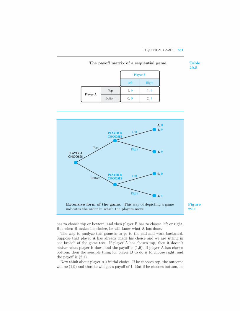
SEQUENTIAL GAMES 551
Player B
Player ATop
Bottom
1, 9
0, 0
1, 9
2, 1
Left Right
The payoff matrix of a sequential game. Table29.5
Bottom
TopRight
Left
Right
Left
1, 9
1, 9
0, 0
2, 1
PLAYER BCHOOSES
PLAYER BCHOOSES
PLAYER ACHOOSES
A, B
Extensive form of the game. This way of depicting a gameindicates the order in which the players move.
Figure29.1
has to choose top or bottom, and then player B has to choose left or right.But when B makes his choice, he will know what A has done.
The way to analyze this game is to go to the end and work backward.Suppose that player A has already made his choice and we are sitting inone branch of the game tree. If player A has chosen top, then it doesn’tmatter what player B does, and the payoff is (1,9). If player A has chosenbottom, then the sensible thing for player B to do is to choose right, andthe payoff is (2,1).
Now think about player A’s initial choice. If he chooses top, the outcomewill be (1,9) and thus he will get a payoff of 1. But if he chooses bottom, he
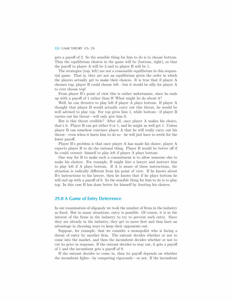
552 GAME THEORY (Ch. 29)
gets a payoff of 2. So the sensible thing for him to do is to choose bottom.Thus the equilibrium choices in the game will be (bottom, right), so thatthe payoff to player A will be 2 and to player B will be 1.The strategies (top, left) are not a reasonable equilibrium in this sequen-
tial game. That is, they are not an equilibrium given the order in whichthe players actually get to make their choices. It is true that if player Achooses top, player B could choose left—but it would be silly for player Ato ever choose top!From player B’s point of view this is rather unfortunate, since he ends
up with a payoff of 1 rather than 9! What might he do about it?Well, he can threaten to play left if player A plays bottom. If player A
thought that player B would actually carry out this threat, he would bewell advised to play top. For top gives him 1, while bottom—if player Bcarries out his threat—will only give him 0.But is this threat credible? After all, once player A makes his choice,
that’s it. Player B can get either 0 or 1, and he might as well get 1. Unlessplayer B can somehow convince player A that he will really carry out histhreat—even when it hurts him to do so—he will just have to settle for thelower payoff.Player B’s problem is that once player A has made his choice, player A
expects player B to do the rational thing. Player B would be better off ifhe could commit himself to play left if player A plays bottom.
One way for B to make such a commitment is to allow someone else tomake his choices. For example, B might hire a lawyer and instruct himto play left if A plays bottom. If A is aware of these instructions, thesituation is radically different from his point of view. If he knows aboutB’s instructions to his lawyer, then he knows that if he plays bottom hewill end up with a payoff of 0. So the sensible thing for him to do is to playtop. In this case B has done better for himself by limiting his choices.
29.8 A Game of Entry Deterrence
In our examination of oligopoly we took the number of firms in the industryas fixed. But in many situations, entry is possible. Of course, it is in theinterest of the firms in the industry to try to prevent such entry. Sincethey are already in the industry, they get to move first and thus have anadvantage in choosing ways to keep their opponents out.Suppose, for example, that we consider a monopolist who is facing a
threat of entry by another firm. The entrant decides whether or not tocome into the market, and then the incumbent decides whether or not tocut its price in response. If the entrant decides to stay out, it gets a payoffof 1 and the incumbent gets a payoff of 9.If the entrant decides to come in, then its payoff depends on whether
the incumbent fights—by competing vigorously—or not. If the incumbent
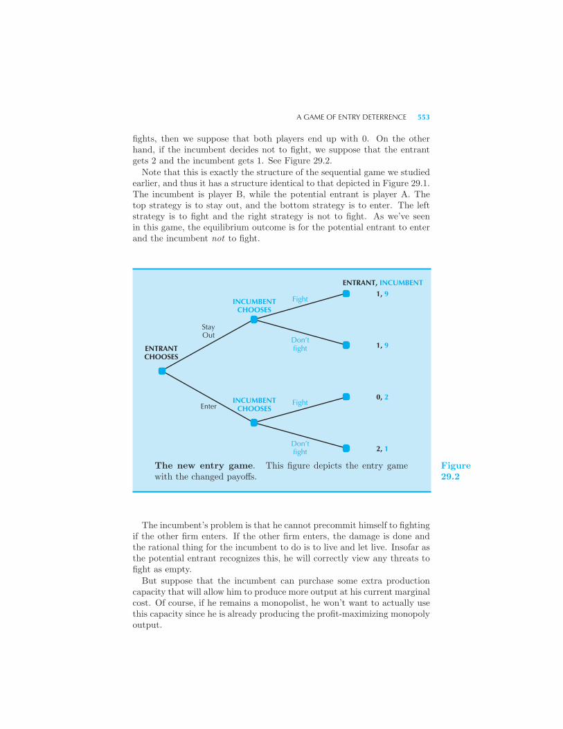
A GAME OF ENTRY DETERRENCE 553
fights, then we suppose that both players end up with 0. On the otherhand, if the incumbent decides not to fight, we suppose that the entrantgets 2 and the incumbent gets 1. See Figure 29.2.
Note that this is exactly the structure of the sequential game we studiedearlier, and thus it has a structure identical to that depicted in Figure 29.1.The incumbent is player B, while the potential entrant is player A. Thetop strategy is to stay out, and the bottom strategy is to enter. The leftstrategy is to fight and the right strategy is not to fight. As we’ve seenin this game, the equilibrium outcome is for the potential entrant to enterand the incumbent not to fight.
1, 9
1, 9
Enter
StayOut
Don’tfight
Fight
0, 2
2, 1 Don’tfight
Fight
INCUMBENTCHOOSES
INCUMBENTCHOOSES
ENTRANTCHOOSES
ENTRANT, INCUMBENT
The new entry game. This figure depicts the entry gamewith the changed payoffs.
Figure29.2
The incumbent’s problem is that he cannot precommit himself to fightingif the other firm enters. If the other firm enters, the damage is done andthe rational thing for the incumbent to do is to live and let live. Insofar asthe potential entrant recognizes this, he will correctly view any threats tofight as empty.
But suppose that the incumbent can purchase some extra productioncapacity that will allow him to produce more output at his current marginalcost. Of course, if he remains a monopolist, he won’t want to actually usethis capacity since he is already producing the profit-maximizing monopolyoutput.
554 GAME THEORY (Ch. 29)
But, if the other firm enters, the incumbent will now be able to produceso much output that he may well be able to compete much more successfullyagainst the new entrant. By investing in the extra capacity, he will lowerhis costs of fighting if the other firm tries to enter. Let us assume that ifhe purchases the extra capacity and if he chooses to fight, he will make aprofit of 2. This changes the game tree to the form depicted in .Now, because of the increased capacity, the threat of fighting is credible.
If the potential entrant comes into the market, the incumbent will get apayoff of 2 if he fights and 1 if he doesn’t; thus the incumbent will rationallychoose to fight. The entrant will therefore get a payoff of 0 if he enters, andif he stays out he will get a payoff of 1. The sensible thing for the potentialentrant to do is to stay out.But this means that the incumbent will remain a monopolist and never
have to use his extra capacity! Despite this, it is worthwhile for the mo-nopolist to invest in the extra capacity in order to make credible the threatof fighting if a new firm tries to enter the market. By investing in “excess”capacity, the monopolist has signaled to the potential entrant that he willbe able to successfully defend his market.
Summary
1. A game can be described by indicating the payoffs to each of the playersfor each configuration of strategic choices they make.
2. A dominant strategy equilibrium is a set of choices for which eachplayer’s choices are optimal regardless of what the other players choose.
3. A Nash equilibrium is a set of choices for which each player’s choice isoptimal, given the choices of the other players.
4. The prisoner’s dilemma is a particular game in which the Pareto efficientoutcome is strategically dominated by an inefficient outcome.
5. If a prisoner’s dilemma is repeated an indefinite number of times, thenit is possible that the Pareto efficient outcome may result from rationalplay.
6. In a sequential game, the time pattern of choices is important. In thesegames, it can often be advantageous to find a way to precommit to aparticular line of play.
REVIEW QUESTIONS 555
REVIEW QUESTIONS
1. Consider the tit-for-tat strategy in the repeated prisoner’s dilemma.Suppose that one player makes a mistake and defects when he meant tocooperate. If both players continue to play tit for tat after that, whathappens?
2. Are dominant strategy equilibria always Nash equilibria? Are Nashequilibria always dominant strategy equilibria?
3. Suppose your opponent is not playing her Nash equilibrium strategy.Should you play your Nash equilibrium strategy?
4. We know that the single-shot prisoner’s dilemma game results in a domi-nant Nash equilibrium strategy that is Pareto inefficient. Suppose we allowthe two prisoners to retaliate after their respective prison terms. Formally,what aspect of the game would this affect? Could a Pareto efficient outcomeresult?
5. What is the dominant Nash equilibrium strategy for the repeated pris-oner’s dilemma game when both players know that the game will end afterone million repetitions? If you were going to run an experiment with hu-man players for such a scenario, would you predict that players would usethis strategy?
6. Suppose that player B rather than player A gets to move first in thesequential game described in this chapter. Draw the extensive form of thenew game. What is the equilibrium for this game? Does player B prefer tomove first or second?

CHAPTER 30
GAMEAPPLICATIONS
In the last chapter we described a number of important concepts in gametheory and illustrated them using a few examples. In this chapter weexamine four important issues in game theory—cooperation, competition,coexistence, and commitment—and see how they work in various strategicinteractions.In order to do this, we first develop an important analytic tool, best
response curves, which can be used to solve for equilibria in games.
30.1 Best Response Curves
Consider a two-person game, and put yourself in the position of one of theplayers. For any choice the other player can make, your best responseis the choice that maximizes your payoff. If there are several choices thatmaximize your payoff, then your best response will be the set of all suchchoices.For example, consider the game depicted in Table 30.1, which we used to
illustrate the concept of a Nash equilibrium. If the column player choosesleft, row’s best response is to choose top; if column chooses right, then
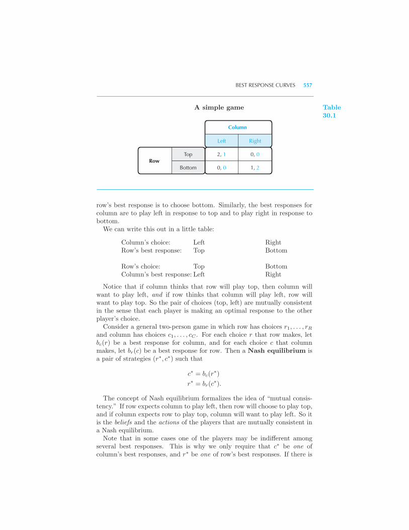
BEST RESPONSE CURVES 557
Column
RowTop
Bottom
2, 1
0, 0
0, 0
1, 2
Left Right
A simple game Table30.1
row’s best response is to choose bottom. Similarly, the best responses forcolumn are to play left in response to top and to play right in response tobottom.We can write this out in a little table:
Column’s choice: Left RightRow’s best response: Top Bottom
Row’s choice: Top BottomColumn’s best response: Left Right
Notice that if column thinks that row will play top, then column willwant to play left, and if row thinks that column will play left, row willwant to play top. So the pair of choices (top, left) are mutually consistentin the sense that each player is making an optimal response to the otherplayer’s choice.Consider a general two-person game in which row has choices r1, . . . , rR
and column has choices c1, . . . , cC . For each choice r that row makes, letbc(r) be a best response for column, and for each choice c that columnmakes, let br(c) be a best response for row. Then a Nash equilibrium isa pair of strategies (r∗, c∗) such that
c∗ = bc(r∗)
r∗ = br(c∗).
The concept of Nash equilibrium formalizes the idea of “mutual consis-tency.” If row expects column to play left, then row will choose to play top,and if column expects row to play top, column will want to play left. So itis the beliefs and the actions of the players that are mutually consistent ina Nash equilibrium.Note that in some cases one of the players may be indifferent among
several best responses. This is why we only require that c∗ be one ofcolumn’s best responses, and r∗ be one of row’s best responses. If there is
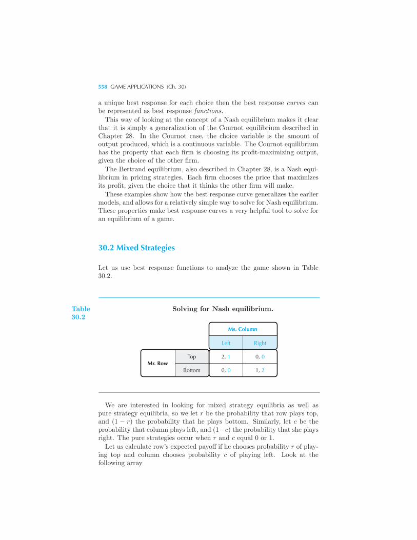
558 GAME APPLICATIONS (Ch. 30)
a unique best response for each choice then the best response curves canbe represented as best response functions.
This way of looking at the concept of a Nash equilibrium makes it clearthat it is simply a generalization of the Cournot equilibrium described inChapter 28. In the Cournot case, the choice variable is the amount ofoutput produced, which is a continuous variable. The Cournot equilibriumhas the property that each firm is choosing its profit-maximizing output,given the choice of the other firm.
The Bertrand equilibrium, also described in Chapter 28, is a Nash equi-librium in pricing strategies. Each firm chooses the price that maximizesits profit, given the choice that it thinks the other firm will make.
These examples show how the best response curve generalizes the earliermodels, and allows for a relatively simple way to solve for Nash equilibrium.These properties make best response curves a very helpful tool to solve foran equilibrium of a game.
30.2 Mixed Strategies
Let us use best response functions to analyze the game shown in Table30.2.
Ms. Column
Mr. RowTop
Bottom
2, 1
0, 0
0, 0
1, 2
Left Right
Table30.2
Solving for Nash equilibrium.
We are interested in looking for mixed strategy equilibria as well aspure strategy equilibria, so we let r be the probability that row plays top,and (1 − r) the probability that he plays bottom. Similarly, let c be theprobability that column plays left, and (1−c) the probability that she playsright. The pure strategies occur when r and c equal 0 or 1.
Let us calculate row’s expected payoff if he chooses probability r of play-ing top and column chooses probability c of playing left. Look at thefollowing array
MIXED STRATEGIES 559
Combination Probability Payoff to RowTop, Left rc 2Bottom, Left (1− r)c 0Top, Right r(1− c) 0Bottom, Right (1− r)(1− c) 1
To calculate the expected payoff to row, we weight row’s payoffs in thethird column by the probability that they occur, given in the second col-umn, and add these up. The answer is
Row’s payoff = 2rc+ (1− r)(1− c),
which we can multiply out to be
Row’s payoff = 2rc+ 1− r − c+ rc.
Now suppose that row contemplates increasing r by Δr. How will hispayoff change?
Δpayoff to row = 2cΔr −Δr + cΔr
= (3c− 1)Δr.
This expression will be positive when 3c > 1 and negative when 3c < 1.Hence, row will want to increase r whenever c > 1/3, decrease r whenc < 1/3, and be happy with any value of 0 ≤ r ≤ 1 when c = 1/3.
Similarly, the payoff to column is given by
Column’s payoff = cr + 2(1− c)(1− r).
Column’s payoff will change when c changes by Δc according to
Δpayoff to column = rΔc+ 2rΔc− 2Δc
= (3r − 2)Δc.
Hence column will want to increase c whenever r > 2/3, decrease c whenr < 2/3, and be happy with any value of 0 ≤ c ≤ 1 when r = 2/3.
We can use this information to plot the best response curves. Start withrow. If column choses c = 0, row will want to make r as small as possible,so r = 0 is the best response to c = 0. This choice will continue to be thebest response up until c = 1/3, at which point any value of r between 0and 1 is a best response. For all c > 1/3, the best response row can makeis r = 1.These curves are depicted in Figure 30.1. It is easy to see that they cross
in three places: (0, 0), (2/3, 1/3), and (1, 1), which correspond to the threeNash equilibria of this game. Two of these strategies are pure strategies,and one is a mixed strategy.

560 GAME APPLICATIONS (Ch. 30)
0 2/3 1
1c
1/3
Row’s bestresponse
Column’s bestresponse
r
Figure30.1
Best response curves. The two curves depict the best re-sponse of row and column to each other’s choices. The inter-sections of the curves are Nash equilibria. In this case there arethree equilibria, two with pure strategies and one with mixedstrategies.
30.3 Games of Coordination
Armed with the tools of the last section we can examine our first class ofgames, coordination games. These are games where the payoffs to theplayers are highest when they can coordinate their strategies. The problem,in practice, is to develop mechanisms that enable this coordination.
Battle of the Sexes
The classic example of a coordination game is the so-called battle of thesexes. In this game, a boy and a girl want to meet at a movie but haven’thad a chance to arrange which one. Alas, they forgot their cell phones,so they have no way to coordinate their meeting and have to guess whichmovie the other will want to attend.The boy wants to see the latest action flick, while the girl would rather
go to an art film, but they would both rather go to the same movie thannot meet up at all. Payoffs consistent with these preferences are shown in
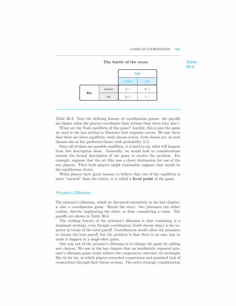
GAMES OF COORDINATION 561
Girl
BoyAction
Art
2, 1
0, 0
0, 0
1, 2
Action Art
The battle of the sexes. Table30.3
Table 30.3. Note the defining feature of coordination games: the payoffsare higher when the players coordinate their actions than when they don’t.What are the Nash equilibria of this game? Luckily, this is just the game
we used in the last section to illustrate best response curves. We saw therethat there are three equilibria: both choose action, both choose art, or eachchooses his or her preferred choice with probability 2/3.Since all of these are possible equilibria, it is hard to say what will happen
from this description alone. Generally, we would look to considerationsoutside the formal description of the game to resolve the problem. Forexample, suppose that the art film was a closer destination for one of thetwo players. Then both players might reasonably suppose that would bethe equilibrium choice.When players have good reasons to believe that one of the equilibria is
more “natural” than the others, it is called a focal point of the game.
Prisoner’s Dilemma
The prisoner’s dilemma, which we discussed extensively in the last chapter,is also a coordination game. Recall the story: two prisoners can eitherconfess, thereby implicating the other, or deny committing a crime. Thepayoffs are shown in Table 30.4.The striking feature of the prisoner’s dilemma is that confessing is a
dominant strategy, even though coordination (both choose deny) is far su-perior in terms of the total payoff. Coordination would allow the prisonersto choose the best payoff, but the problem is that there is no easy way tomake it happen in a single-shot game.One way out of the prisoner’s dilemma is to enlarge the game by adding
new choices. We saw in the last chapter that an indefinitely repeated pris-oner’s dilemma game could achieve the cooperative outcome via strategieslike tit for tat, in which players rewarded cooperation and punished lack ofcooperation through their future actions. The extra strategic consideration
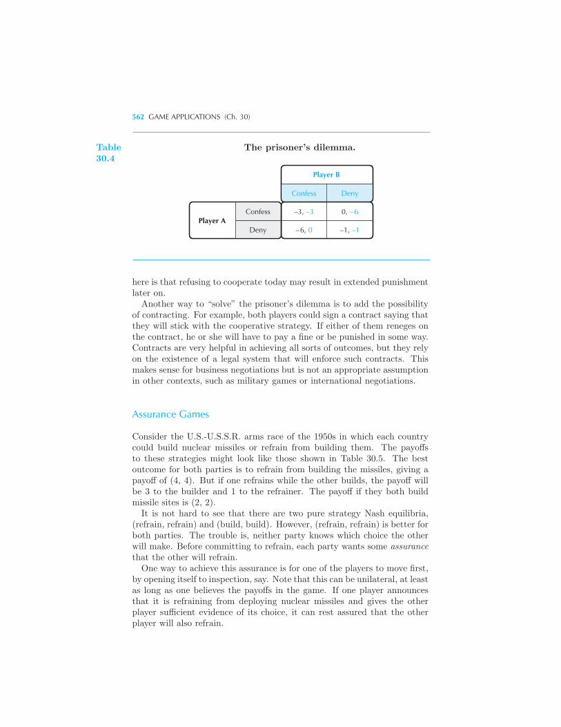
562 GAME APPLICATIONS (Ch. 30)
Player B
Player AConfess
Deny
–3, –3
–6, 0
0, –6
–1, –1
Confess Deny
Table30.4
The prisoner’s dilemma.
here is that refusing to cooperate today may result in extended punishmentlater on.Another way to “solve” the prisoner’s dilemma is to add the possibility
of contracting. For example, both players could sign a contract saying thatthey will stick with the cooperative strategy. If either of them reneges onthe contract, he or she will have to pay a fine or be punished in some way.Contracts are very helpful in achieving all sorts of outcomes, but they relyon the existence of a legal system that will enforce such contracts. Thismakes sense for business negotiations but is not an appropriate assumptionin other contexts, such as military games or international negotiations.
Assurance Games
Consider the U.S.-U.S.S.R. arms race of the 1950s in which each countrycould build nuclear missiles or refrain from building them. The payoffsto these strategies might look like those shown in Table 30.5. The bestoutcome for both parties is to refrain from building the missiles, giving apayoff of (4, 4). But if one refrains while the other builds, the payoff willbe 3 to the builder and 1 to the refrainer. The payoff if they both buildmissile sites is (2, 2).It is not hard to see that there are two pure strategy Nash equilibria,
(refrain, refrain) and (build, build). However, (refrain, refrain) is better forboth parties. The trouble is, neither party knows which choice the otherwill make. Before committing to refrain, each party wants some assurancethat the other will refrain.One way to achieve this assurance is for one of the players to move first,
by opening itself to inspection, say. Note that this can be unilateral, at leastas long as one believes the payoffs in the game. If one player announcesthat it is refraining from deploying nuclear missiles and gives the otherplayer sufficient evidence of its choice, it can rest assured that the otherplayer will also refrain.
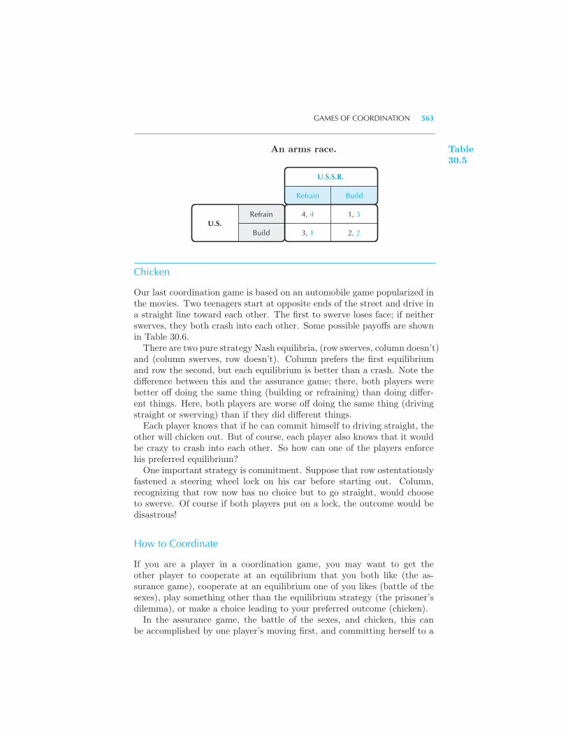
GAMES OF COORDINATION 563
U.S.S.R.
U.S.Refrain
Build
4, 4
3, 1
1, 3
2, 2
Refrain Build
An arms race. Table30.5
Chicken
Our last coordination game is based on an automobile game popularized inthe movies. Two teenagers start at opposite ends of the street and drive ina straight line toward each other. The first to swerve loses face; if neitherswerves, they both crash into each other. Some possible payoffs are shownin Table 30.6.There are two pure strategy Nash equilibria, (row swerves, column doesn’t)
and (column swerves, row doesn’t). Column prefers the first equilibriumand row the second, but each equilibrium is better than a crash. Note thedifference between this and the assurance game; there, both players werebetter off doing the same thing (building or refraining) than doing differ-ent things. Here, both players are worse off doing the same thing (drivingstraight or swerving) than if they did different things.Each player knows that if he can commit himself to driving straight, the
other will chicken out. But of course, each player also knows that it wouldbe crazy to crash into each other. So how can one of the players enforcehis preferred equilibrium?One important strategy is commitment. Suppose that row ostentatiously
fastened a steering wheel lock on his car before starting out. Column,recognizing that row now has no choice but to go straight, would chooseto swerve. Of course if both players put on a lock, the outcome would bedisastrous!
How to Coordinate
If you are a player in a coordination game, you may want to get theother player to cooperate at an equilibrium that you both like (the as-surance game), cooperate at an equilibrium one of you likes (battle of thesexes), play something other than the equilibrium strategy (the prisoner’sdilemma), or make a choice leading to your preferred outcome (chicken).In the assurance game, the battle of the sexes, and chicken, this can
be accomplished by one player’s moving first, and committing herself to a
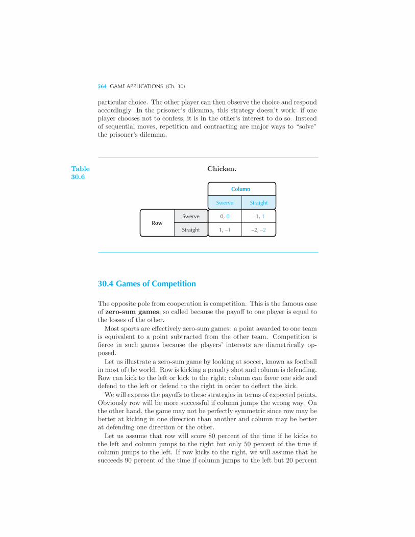
564 GAME APPLICATIONS (Ch. 30)
particular choice. The other player can then observe the choice and respondaccordingly. In the prisoner’s dilemma, this strategy doesn’t work: if oneplayer chooses not to confess, it is in the other’s interest to do so. Insteadof sequential moves, repetition and contracting are major ways to “solve”the prisoner’s dilemma.
Column
RowSwerve
Straight
0, 0
1, –1
–1, 1
–2, –2
Swerve Straight
Table30.6
Chicken.
30.4 Games of Competition
The opposite pole from cooperation is competition. This is the famous caseof zero-sum games, so called because the payoff to one player is equal tothe losses of the other.
Most sports are effectively zero-sum games: a point awarded to one teamis equivalent to a point subtracted from the other team. Competition isfierce in such games because the players’ interests are diametrically op-posed.
Let us illustrate a zero-sum game by looking at soccer, known as footballin most of the world. Row is kicking a penalty shot and column is defending.Row can kick to the left or kick to the right; column can favor one side anddefend to the left or defend to the right in order to deflect the kick.
We will express the payoffs to these strategies in terms of expected points.Obviously row will be more successful if column jumps the wrong way. Onthe other hand, the game may not be perfectly symmetric since row may bebetter at kicking in one direction than another and column may be betterat defending one direction or the other.
Let us assume that row will score 80 percent of the time if he kicks tothe left and column jumps to the right but only 50 percent of the time ifcolumn jumps to the left. If row kicks to the right, we will assume that hesucceeds 90 percent of the time if column jumps to the left but 20 percent
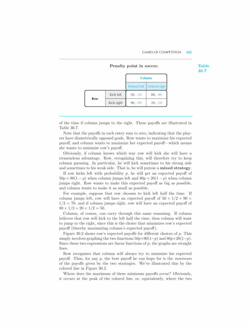
GAMES OF COMPETITION 565
Column
RowKick left
Kick right
50, –50
90, –90
80, –80
20, –20
Defend left Defend right
Penalty point in soccer. Table30.7
of the time if column jumps to the right. These payoffs are illustrated inTable 30.7.
Note that the payoffs in each entry sum to zero, indicating that the play-ers have diametrically opposed goals. Row wants to maximize his expectedpayoff, and column wants to maximize her expected payoff—which meansshe wants to minimize row’s payoff.
Obviously, if column knows which way row will kick she will have atremendous advantage. Row, recognizing this, will therefore try to keepcolumn guessing. In particular, he will kick sometimes to his strong sideand sometimes to his weak side. That is, he will pursue a mixed strategy.
If row kicks left with probability p, he will get an expected payoff of50p+ 90(1− p) when column jumps left and 80p+ 20(1− p) when columnjumps right. Row wants to make this expected payoff as big as possible,and column wants to make it as small as possible.
For example, suppose that row chooses to kick left half the time. Ifcolumn jumps left, row will have an expected payoff of 50 × 1/2 + 90 ×1/2 = 70, and if column jumps right, row will have an expected payoff of80× 1/2 + 20× 1/2 = 50.
Column, of course, can carry through this same reasoning. If columnbelieves that row will kick to the left half the time, then column will wantto jump to the right, since this is the choice that minimizes row’s expectedpayoff (thereby maximizing column’s expected payoff).
Figure 30.2 shows row’s expected payoffs for different choices of p. Thissimply involves graphing the two functions 50p+90(1−p) and 80p+20(1−p).Since these two expressions are linear functions of p, the graphs are straightlines.
Row recognizes that column will always try to minimize his expectedpayoff. Thus, for any p, the best payoff he can hope for is the minimumof the payoffs given by the two strategies. We’ve illustrated this by thecolored line in Figure 30.2.
Where does the maximum of these minimum payoffs occur? Obviously,it occurs at the peak of the colored line, or, equivalently, where the two
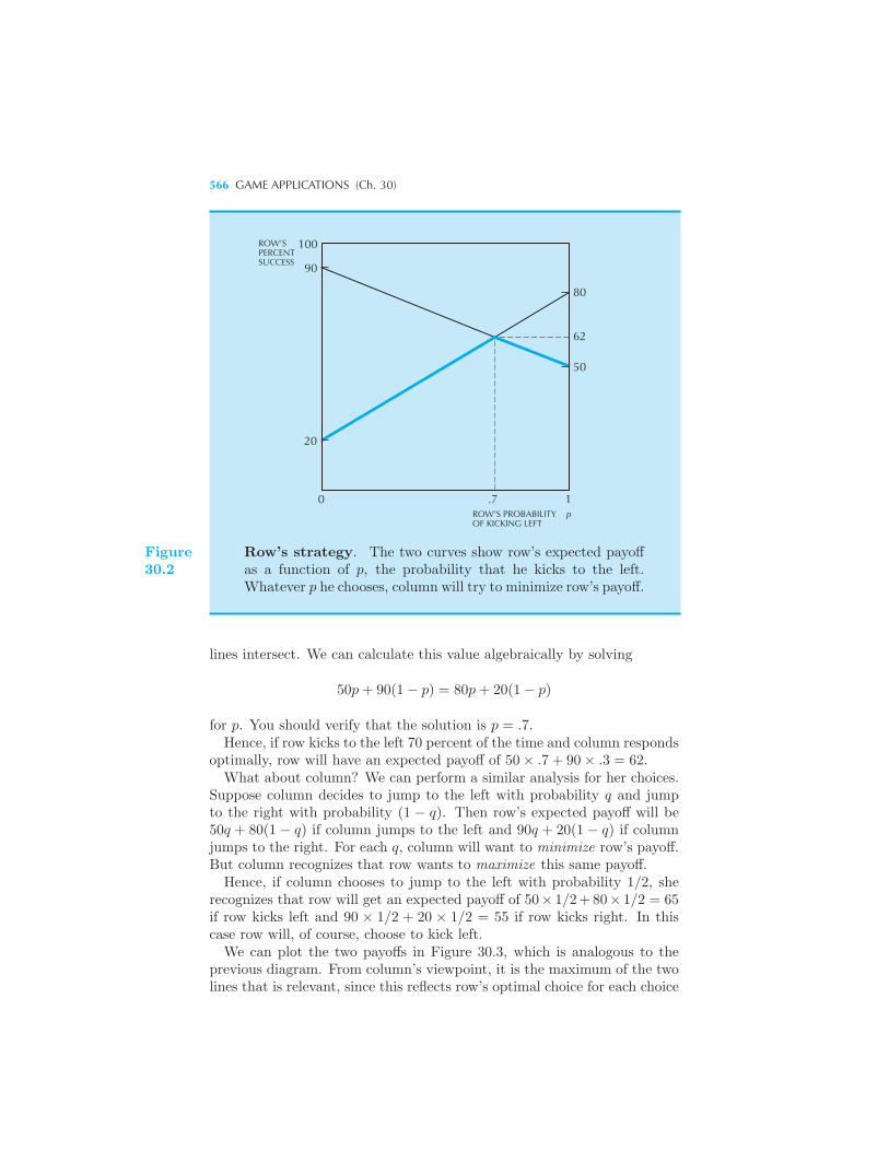
566 GAME APPLICATIONS (Ch. 30)
0 .7 1ROW’S PROBABILITY p OF KICKING LEFT
100
90
ROW’SPERCENTSUCCESS
20
80
62
50
Figure30.2
Row’s strategy. The two curves show row’s expected payoffas a function of p, the probability that he kicks to the left.Whatever p he chooses, column will try to minimize row’s payoff.
lines intersect. We can calculate this value algebraically by solving
50p+ 90(1− p) = 80p+ 20(1− p)
for p. You should verify that the solution is p = .7.Hence, if row kicks to the left 70 percent of the time and column responds
optimally, row will have an expected payoff of 50× .7 + 90× .3 = 62.What about column? We can perform a similar analysis for her choices.
Suppose column decides to jump to the left with probability q and jumpto the right with probability (1 − q). Then row’s expected payoff will be50q + 80(1 − q) if column jumps to the left and 90q + 20(1 − q) if columnjumps to the right. For each q, column will want to minimize row’s payoff.But column recognizes that row wants to maximize this same payoff.Hence, if column chooses to jump to the left with probability 1/2, she
recognizes that row will get an expected payoff of 50× 1/2+80× 1/2 = 65if row kicks left and 90 × 1/2 + 20 × 1/2 = 55 if row kicks right. In thiscase row will, of course, choose to kick left.We can plot the two payoffs in Figure 30.3, which is analogous to the
previous diagram. From column’s viewpoint, it is the maximum of the twolines that is relevant, since this reflects row’s optimal choice for each choice
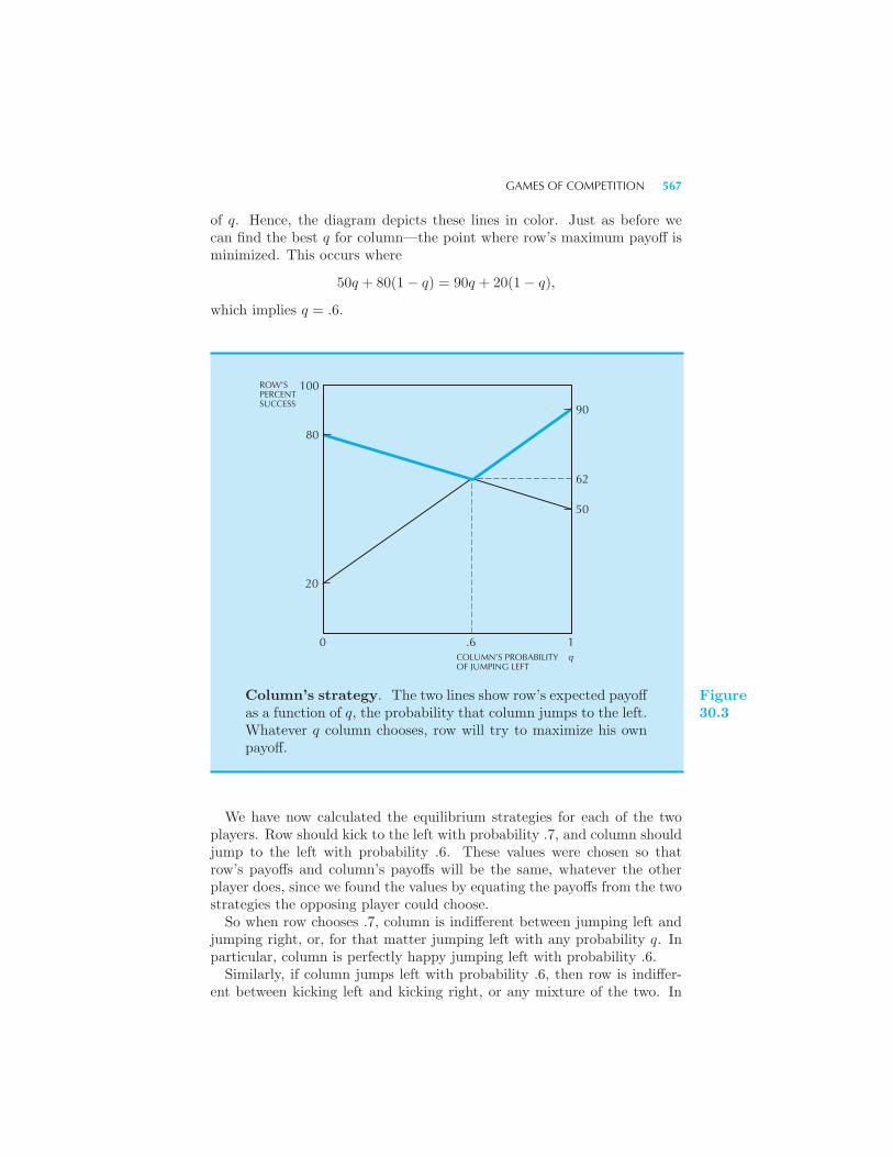
GAMES OF COMPETITION 567
of q. Hence, the diagram depicts these lines in color. Just as before wecan find the best q for column—the point where row’s maximum payoff isminimized. This occurs where
50q + 80(1− q) = 90q + 20(1− q),
which implies q = .6.
0 .6 1
ROW’SPERCENTSUCCESS
20
62
50
100
80
90
COLUMN’S PROBABILITY q OF JUMPING LEFT
Column’s strategy. The two lines show row’s expected payoffas a function of q, the probability that column jumps to the left.Whatever q column chooses, row will try to maximize his ownpayoff.
Figure30.3
We have now calculated the equilibrium strategies for each of the twoplayers. Row should kick to the left with probability .7, and column shouldjump to the left with probability .6. These values were chosen so thatrow’s payoffs and column’s payoffs will be the same, whatever the otherplayer does, since we found the values by equating the payoffs from the twostrategies the opposing player could choose.So when row chooses .7, column is indifferent between jumping left and
jumping right, or, for that matter jumping left with any probability q. Inparticular, column is perfectly happy jumping left with probability .6.Similarly, if column jumps left with probability .6, then row is indiffer-
ent between kicking left and kicking right, or any mixture of the two. In
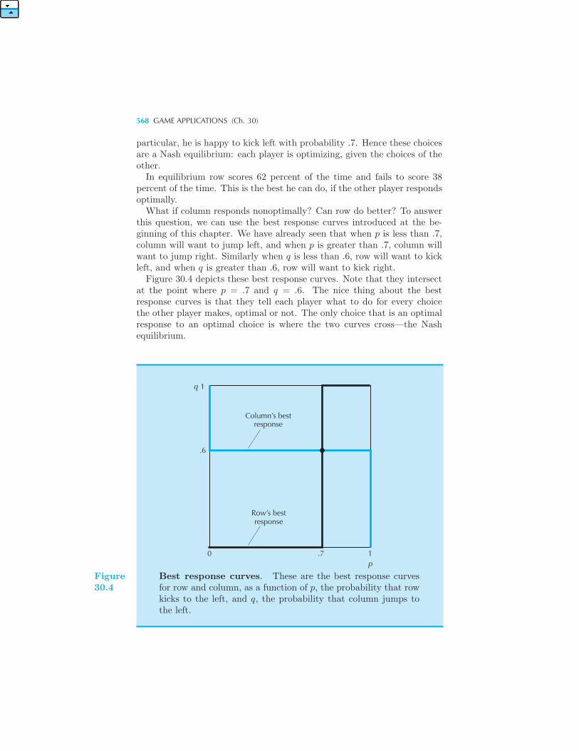
568 GAME APPLICATIONS (Ch. 30)
particular, he is happy to kick left with probability .7. Hence these choicesare a Nash equilibrium: each player is optimizing, given the choices of theother.In equilibrium row scores 62 percent of the time and fails to score 38
percent of the time. This is the best he can do, if the other player respondsoptimally.What if column responds nonoptimally? Can row do better? To answer
this question, we can use the best response curves introduced at the be-ginning of this chapter. We have already seen that when p is less than .7,column will want to jump left, and when p is greater than .7, column willwant to jump right. Similarly when q is less than .6, row will want to kickleft, and when q is greater than .6, row will want to kick right.
Figure 30.4 depicts these best response curves. Note that they intersectat the point where p = .7 and q = .6. The nice thing about the bestresponse curves is that they tell each player what to do for every choicethe other player makes, optimal or not. The only choice that is an optimalresponse to an optimal choice is where the two curves cross—the Nashequilibrium.
Column’s bestresponse
Row’s bestresponse
0 .7 1p
.6
1q
Figure30.4
Best response curves. These are the best response curvesfor row and column, as a function of p, the probability that rowkicks to the left, and q, the probability that column jumps tothe left.
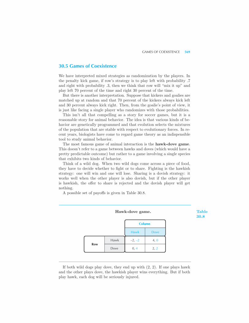
GAMES OF COEXISTENCE 569
30.5 Games of Coexistence
We have interpreted mixed strategies as randomization by the players. Inthe penalty kick game, if row’s strategy is to play left with probability .7and right with probability .3, then we think that row will “mix it up” andplay left 70 percent of the time and right 30 percent of the time.But there is another interpretation. Suppose that kickers and goalies are
matched up at random and that 70 percent of the kickers always kick leftand 30 percent always kick right. Then, from the goalie’s point of view, itis just like facing a single player who randomizes with those probabilities.This isn’t all that compelling as a story for soccer games, but it is a
reasonable story for animal behavior. The idea is that various kinds of be-havior are genetically programmed and that evolution selects the mixturesof the population that are stable with respect to evolutionary forces. In re-cent years, biologists have come to regard game theory as an indispensibletool to study animal behavior.The most famous game of animal interaction is the hawk-dove game.
This doesn’t refer to a game between hawks and doves (which would have apretty predictable outcome) but rather to a game involving a single speciesthat exhibits two kinds of behavior.Think of a wild dog. When two wild dogs come across a piece of food,
they have to decide whether to fight or to share. Fighting is the hawkishstrategy: one will win and one will lose. Sharing is a dovish strategy: itworks well when the other player is also dovish, but if the other playeris hawkish, the offer to share is rejected and the dovish player will getnothing.A possible set of payoffs is given in Table 30.8.
Column
RowHawk
Dove
–2, –2
0, 4
4, 0
2, 2
Hawk Dove
Hawk-dove game. Table30.8
If both wild dogs play dove, they end up with (2, 2). If one plays hawkand the other plays dove, the hawkish player wins everything. But if bothplay hawk, each dog will be seriously injured.
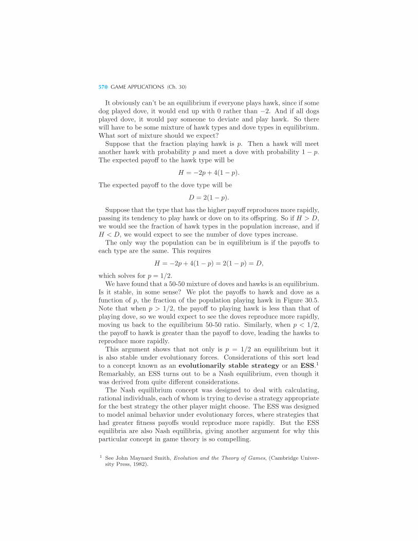
570 GAME APPLICATIONS (Ch. 30)
It obviously can’t be an equilibrium if everyone plays hawk, since if somedog played dove, it would end up with 0 rather than −2. And if all dogsplayed dove, it would pay someone to deviate and play hawk. So therewill have to be some mixture of hawk types and dove types in equilibrium.What sort of mixture should we expect?Suppose that the fraction playing hawk is p. Then a hawk will meet
another hawk with probability p and meet a dove with probability 1 − p.The expected payoff to the hawk type will be
H = −2p+ 4(1− p).
The expected payoff to the dove type will be
D = 2(1− p).
Suppose that the type that has the higher payoff reproduces more rapidly,passing its tendency to play hawk or dove on to its offspring. So if H > D,we would see the fraction of hawk types in the population increase, and ifH < D, we would expect to see the number of dove types increase.The only way the population can be in equilibrium is if the payoffs to
each type are the same. This requires
H = −2p+ 4(1− p) = 2(1− p) = D,
which solves for p = 1/2.We have found that a 50-50 mixture of doves and hawks is an equilibrium.
Is it stable, in some sense? We plot the payoffs to hawk and dove as afunction of p, the fraction of the population playing hawk in Figure 30.5.Note that when p > 1/2, the payoff to playing hawk is less than that ofplaying dove, so we would expect to see the doves reproduce more rapidly,moving us back to the equilibrium 50-50 ratio. Similarly, when p < 1/2,the payoff to hawk is greater than the payoff to dove, leading the hawks toreproduce more rapidly.This argument shows that not only is p = 1/2 an equilibrium but it
is also stable under evolutionary forces. Considerations of this sort leadto a concept known as an evolutionarily stable strategy or an ESS.1
Remarkably, an ESS turns out to be a Nash equilibrium, even though itwas derived from quite different considerations.The Nash equilibrium concept was designed to deal with calculating,
rational individuals, each of whom is trying to devise a strategy appropriatefor the best strategy the other player might choose. The ESS was designedto model animal behavior under evolutionary forces, where strategies thathad greater fitness payoffs would reproduce more rapidly. But the ESSequilibria are also Nash equilibria, giving another argument for why thisparticular concept in game theory is so compelling.
1 See John Maynard Smith, Evolution and the Theory of Games, (Cambridge Univer-sity Press, 1982).
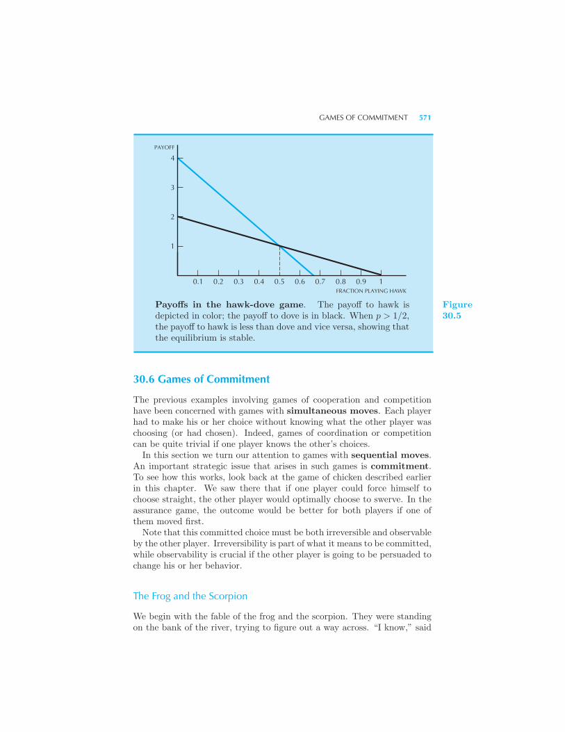
GAMES OF COMMITMENT 571
PAYOFF
FRACTION PLAYING HAWK
4
3
0.20.1 0.4 0.6 0.80.3 0.5 0.7 0.9 1
2
1
Payoffs in the hawk-dove game. The payoff to hawk isdepicted in color; the payoff to dove is in black. When p > 1/2,the payoff to hawk is less than dove and vice versa, showing thatthe equilibrium is stable.
Figure30.5
30.6 Games of Commitment
The previous examples involving games of cooperation and competitionhave been concerned with games with simultaneous moves. Each playerhad to make his or her choice without knowing what the other player waschoosing (or had chosen). Indeed, games of coordination or competitioncan be quite trivial if one player knows the other’s choices.In this section we turn our attention to games with sequential moves.
An important strategic issue that arises in such games is commitment.To see how this works, look back at the game of chicken described earlierin this chapter. We saw there that if one player could force himself tochoose straight, the other player would optimally choose to swerve. In theassurance game, the outcome would be better for both players if one ofthem moved first.Note that this committed choice must be both irreversible and observable
by the other player. Irreversibility is part of what it means to be committed,while observability is crucial if the other player is going to be persuaded tochange his or her behavior.
The Frog and the Scorpion
We begin with the fable of the frog and the scorpion. They were standingon the bank of the river, trying to figure out a way across. “I know,” said
572 GAME APPLICATIONS (Ch. 30)
the scorpion “I will climb on your back and you can swim across the river.”The frog said, “But what if you sting me with your stinger?” The scorpionsaid, “Why would I do that? Then we would both die.”The frog found this convincing, so the scorpion climbed on his back and
they started across the river. Halfway across, at the deepest point, thescorpion stung the frog. Writhing in pain, the frog cried out, “Why didyou do that? Now we are both doomed!” “Alas,” said the scorpion, as hesank into the river, “it is my nature.”Let’s look at the frog and the scorpion from the viewpoint of game theory.
Figure 30.6 depicts a sequential game with payoffs consistent with the story.Start at the bottom of the game tree. If the frog refuses the scorpion,both get nothing. Looking up one line, we see that if the frog carries thescorpion, he receives utility 5, for doing a good deed, and the scorpionreceives a payoff of 3, for getting across the river. In line where the frogis stung, he receives a payoff of −10, and the scorpion gets a payoff of 5,representing the satisfaction from fulfilling his natural instincts.
FROG, SCORPION
–10, 5
5, 3
SCORPIONCHOOSES
Carry
FROGCHOOSES
Refrain
Sting
0, 0
Refuse
Figure30.6
The frog and the scorpion. If the frog chooses to carry thescorpion, the scorpion will choose to sting him and both willdie.
It is best to start with the final move of the game: the scorpion’s choiceof sting or refrain. Stinging has a higher payoff to the scorpion because“it is his nature” to sting. Hence the frog should rationally choose torefuse to carry the scorpion. Unfortunately, the frog didn’t understandthe scorpion’s payoffs; apparently, he thought that the scorpion’s payoffs
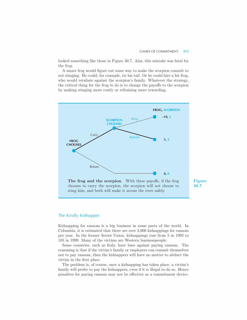
GAMES OF COMMITMENT 573
looked something like those in Figure 30.7. Alas, this mistake was fatal forthe frog.A smart frog would figure out some way to make the scorpion commit to
not stinging. He could, for example, tie his tail. Or he could hire a hit frog,who would retaliate against the scorpion’s family. Whatever the strategy,the critical thing for the frog to do is to change the payoffs to the scorpionby making stinging more costly or refraining more rewarding.
FROG, SCORPION
–10, 2
5, 3
SCORPIONCHOOSES
Refuse
Carry
FROGCHOOSES
Refrain
Sting
0, 0
The frog and the scorpion. With these payoffs, if the frogchooses to carry the scorpion, the scorpion will not choose tosting him, and both will make it across the river safely.
Figure30.7
The Kindly Kidnapper
Kidnapping for ransom is a big business in some parts of the world. InColumbia, it is estimated that there are over 2,000 kidnappings for ransomper year. In the former Soviet Union, kidnappings rose from 5 in 1992 to105 in 1999. Many of the victims are Western businesspeople.Some countries, such as Italy, have laws against paying ransom. The
reasoning is that if the victim’s family or employers can commit themselvesnot to pay ransom, then the kidnappers will have no motive to abduct thevictim in the first place.The problem is, of course, once a kidnapping has taken place, a victim’s
family will prefer to pay the kidnappers, even if it is illegal to do so. Hencepenalties for paying ransom may not be effective as a commitment device.
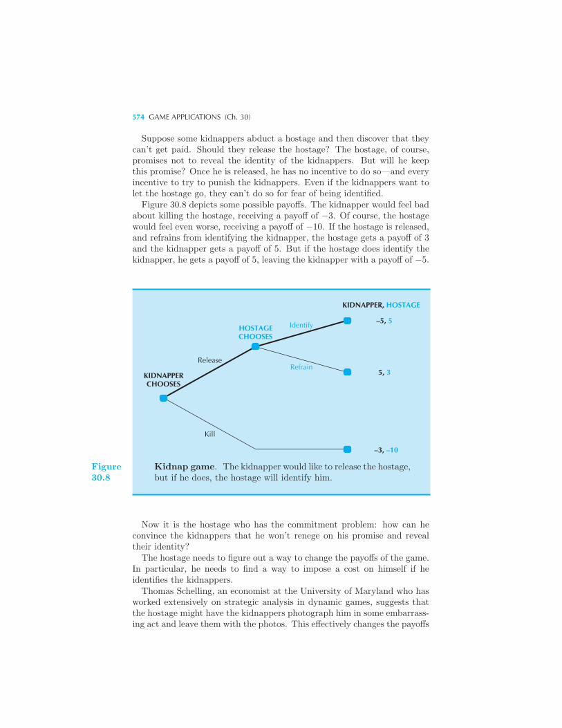
574 GAME APPLICATIONS (Ch. 30)
Suppose some kidnappers abduct a hostage and then discover that theycan’t get paid. Should they release the hostage? The hostage, of course,promises not to reveal the identity of the kidnappers. But will he keepthis promise? Once he is released, he has no incentive to do so—and everyincentive to try to punish the kidnappers. Even if the kidnappers want tolet the hostage go, they can’t do so for fear of being identified.Figure 30.8 depicts some possible payoffs. The kidnapper would feel bad
about killing the hostage, receiving a payoff of −3. Of course, the hostagewould feel even worse, receiving a payoff of −10. If the hostage is released,and refrains from identifying the kidnapper, the hostage gets a payoff of 3and the kidnapper gets a payoff of 5. But if the hostage does identify thekidnapper, he gets a payoff of 5, leaving the kidnapper with a payoff of −5.
KIDNAPPER, HOSTAGE
–5, 5
5, 3
HOSTAGECHOOSES
Kill
Release
KIDNAPPERCHOOSES
Refrain
Identify
–3, –10
Figure30.8
Kidnap game. The kidnapper would like to release the hostage,but if he does, the hostage will identify him.
Now it is the hostage who has the commitment problem: how can heconvince the kidnappers that he won’t renege on his promise and revealtheir identity?The hostage needs to figure out a way to change the payoffs of the game.
In particular, he needs to find a way to impose a cost on himself if heidentifies the kidnappers.Thomas Schelling, an economist at the University of Maryland who has
worked extensively on strategic analysis in dynamic games, suggests thatthe hostage might have the kidnappers photograph him in some embarrass-ing act and leave them with the photos. This effectively changes the payoffs
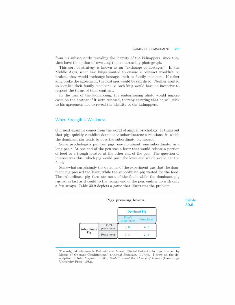
GAMES OF COMMITMENT 575
from his subsequently revealing the identity of the kidnappers, since theythen have the option of revealing the embarrassing photograph.
This sort of strategy is known as an “exchange of hostages.” In theMiddle Ages, when two kings wanted to ensure a contract wouldn’t bebroken, they would exchange hostages such as family members. If eitherking broke the agreement, the hostages would be sacrificed. Neither wantedto sacrifice their family members, so each king would have an incentive torespect the terms of their contract.
In the case of the kidnapping, the embarrassing photo would imposecosts on the hostage if it were released, thereby ensuring that he will stickto his agreement not to reveal the identity of the kidnappers.
When Strength Is Weakness
Our next example comes from the world of animal psychology. It turns outthat pigs quickly establish dominance-subordinateness relations, in whichthe dominant pig tends to boss the subordinate pig around.
Some psychologists put two pigs, one dominant, one subordinate, in along pen.2 At one end of the pen was a lever that would release a portionof food to a trough located at the other end of the pen. The question ofinterest was this: which pig would push the lever and which would eat thefood?
Somewhat surprisingly the outcome of the experiment was that the dom-inant pig pressed the lever, while the subordinate pig waited for the food.The subordinate pig then ate most of the food, while the dominant pigrushed as fast as it could to the trough end of the pen, ending up with onlya few scraps. Table 30.9 depicts a game that illustrates the problem.
Dominant Pig
SubordinatePig
Don’t press lever
Press lever
0, 0
0, 5
4, 1
2, 3
Don’t press lever Press lever
Pigs pressing levers. Table30.9
2 The original reference is Baldwin and Meese, “Social Behavior in Pigs Studied byMeans of Operant Conditioning,” (Animal Behavior, (1979)). I draw on the de-scription of John Maynard Smith, Evolution and the Theory of Games (CambridgeUniversity Press, 1982).
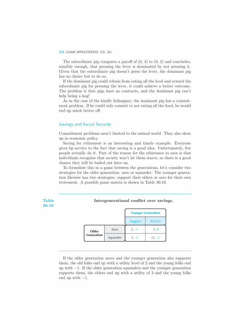
576 GAME APPLICATIONS (Ch. 30)
The subordinate pig compares a payoff of (0, 4) to (0, 2) and concludes,sensibly enough, that pressing the lever is dominated by not pressing it.Given that the subordinate pig doesn’t press the lever, the dominant pighas no choice but to do so.If the dominant pig could refrain from eating all the food and reward the
subordinate pig for pressing the lever, it could achieve a better outcome.The problem is that pigs have no contracts, and the dominant pig can’thelp being a hog!As in the case of the kindly kidnapper, the dominant pig has a commit-
ment problem. If he could only commit to not eating all the food, he wouldend up much better off.
Savings and Social Security
Commitment problems aren’t limited to the animal world. They also showup in economic policy.Saving for retirement is an interesting and timely example. Everyone
gives lip service to the fact that saving is a good idea. Unfortunately, fewpeople actually do it. Part of the reason for the reluctance to save is thatindividuals recognize that society won’t let them starve, so there is a goodchance they will be bailed out later on.To formulate this in a game between the generations, let’s consider two
strategies for the older generation: save or squander. The younger genera-tion likewise has two strategies: support their elders or save for their ownretirement. A possible game matrix is shown in Table 30.10.
Younger Generation
OlderGeneration
Save
Squander
2, –1
–2, –2
1, 0
3, –1
Support Refrain
Table30.10
Intergenerational conflict over savings.
If the older generation saves and the younger generation also supportsthem, the old folks end up with a utility level of 2 and the young folks endup with −1. If the older generation squanders and the younger generationsupports them, the elders end up with a utility of 3 and the young folksend up with −1.
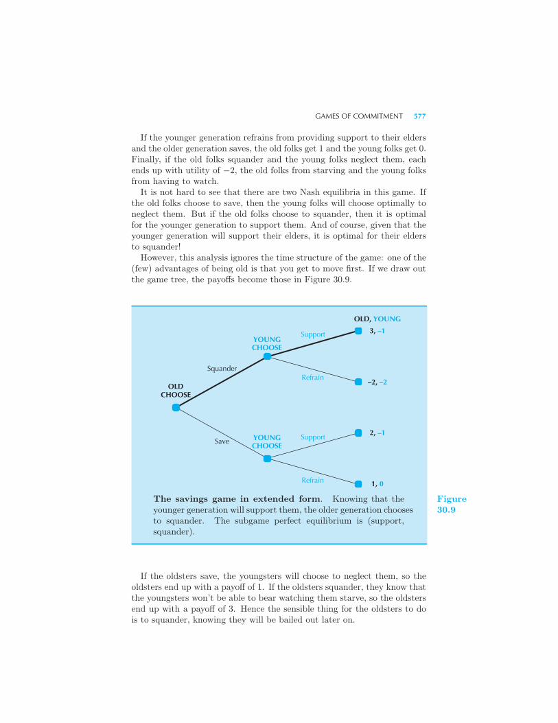
GAMES OF COMMITMENT 577
If the younger generation refrains from providing support to their eldersand the older generation saves, the old folks get 1 and the young folks get 0.Finally, if the old folks squander and the young folks neglect them, eachends up with utility of −2, the old folks from starving and the young folksfrom having to watch.It is not hard to see that there are two Nash equilibria in this game. If
the old folks choose to save, then the young folks will choose optimally toneglect them. But if the old folks choose to squander, then it is optimalfor the younger generation to support them. And of course, given that theyounger generation will support their elders, it is optimal for their eldersto squander!However, this analysis ignores the time structure of the game: one of the
(few) advantages of being old is that you get to move first. If we draw outthe game tree, the payoffs become those in Figure 30.9.
3, –1
–2, –2
Save
Squander
Refrain
Support
YOUNGCHOOSE
YOUNGCHOOSE
OLDCHOOSE
2, –1
1, 0
Refrain
Support
OLD, YOUNG
The savings game in extended form. Knowing that theyounger generation will support them, the older generation choosesto squander. The subgame perfect equilibrium is (support,squander).
Figure30.9
If the oldsters save, the youngsters will choose to neglect them, so theoldsters end up with a payoff of 1. If the oldsters squander, they know thatthe youngsters won’t be able to bear watching them starve, so the oldstersend up with a payoff of 3. Hence the sensible thing for the oldsters to dois to squander, knowing they will be bailed out later on.
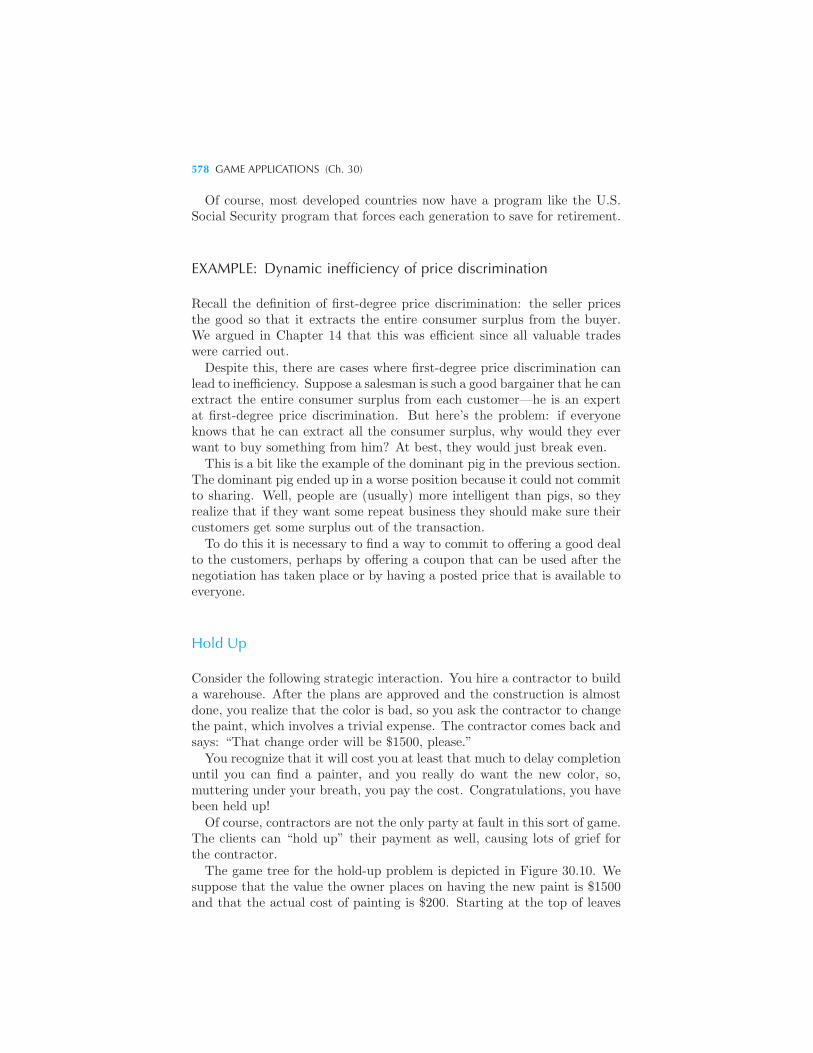
578 GAME APPLICATIONS (Ch. 30)
Of course, most developed countries now have a program like the U.S.Social Security program that forces each generation to save for retirement.
EXAMPLE: Dynamic inefficiency of price discrimination
Recall the definition of first-degree price discrimination: the seller pricesthe good so that it extracts the entire consumer surplus from the buyer.We argued in Chapter 14 that this was efficient since all valuable tradeswere carried out.Despite this, there are cases where first-degree price discrimination can
lead to inefficiency. Suppose a salesman is such a good bargainer that he canextract the entire consumer surplus from each customer—he is an expertat first-degree price discrimination. But here’s the problem: if everyoneknows that he can extract all the consumer surplus, why would they everwant to buy something from him? At best, they would just break even.This is a bit like the example of the dominant pig in the previous section.
The dominant pig ended up in a worse position because it could not committo sharing. Well, people are (usually) more intelligent than pigs, so theyrealize that if they want some repeat business they should make sure theircustomers get some surplus out of the transaction.To do this it is necessary to find a way to commit to offering a good deal
to the customers, perhaps by offering a coupon that can be used after thenegotiation has taken place or by having a posted price that is available toeveryone.
Hold Up
Consider the following strategic interaction. You hire a contractor to builda warehouse. After the plans are approved and the construction is almostdone, you realize that the color is bad, so you ask the contractor to changethe paint, which involves a trivial expense. The contractor comes back andsays: “That change order will be $1500, please.”You recognize that it will cost you at least that much to delay completion
until you can find a painter, and you really do want the new color, so,muttering under your breath, you pay the cost. Congratulations, you havebeen held up!Of course, contractors are not the only party at fault in this sort of game.
The clients can “hold up” their payment as well, causing lots of grief forthe contractor.The game tree for the hold-up problem is depicted in Figure 30.10. We
suppose that the value the owner places on having the new paint is $1500and that the actual cost of painting is $200. Starting at the top of leaves
GAMES OF COMMITMENT 579
of the tree, if the contractor charges $1500, it will realize a profit of $1300,and the client gets a net utility of zero.
If the client looks for another painter, it will cost him $200 to pay thepainter and, say, $1400 in lost time. He gets the color he wants which isworth $1500, buy has to pay $1600 in direct costs and delay costs, leavinghim with a net loss of $100.
If the contractor charges the client the actual cost of $200, he breakseven and the client gets a $1500 value for $200, leaving him with a netpayoff of $1300.
As can be seen, the optimal choice for the contractor is to extort the pay-ment, and the optimal choice for the customer is to give in. But a sensibleclient will recognize that change orders will occur in any project. Becauseof this, the client will be reluctant to hire contractors with a reputation forextortion which is, of course, bad for the contractor.
1300, 0
0, –100
0, 1300
Extort
Chargeactualcost
Find apainter
Givein
CONTRACTORCHOOSES
CLIENTCHOOSES
CONTRACTOR, CLIENT
The hold-up problem. The contractor charges a high pricefor the change since the client has no alternative.
Figure30.10
How do firms solve the hold-up problem? The basic answer is contracts.Normally, contractors negotiate a contract specifying what kinds of changeorders are appropriate and how their costs will be determined. Sometimesthere are even arbitration or other dispute resolution procedures built intothe contracts. A lot of time, energy, and money goes into writing contractsjust to make certain that hold up won’t occur.
But contracts aren’t the only solution. Another way to solve the problemis through commitment. For example, the contractor might post a bond
580 GAME APPLICATIONS (Ch. 30)
guaranteeing timely completion of the project. Again, there will generallybe some objectively specified terms about what constitutes completion.Another important factor is reputation. Obviously, a contractor who
persistently tries to extort his customers will get a bad reputation. Hewon’t be hired again by this customer, and he certainly won’t get goodrecommendations. This reputation effect can be examined in a repeatedgame context in which hold up today will cost the contractor in the future.
30.7 Bargaining
The classical bargaining problem is divide the dollar. Two players have adollar that they want to divide between them. How do they do it?The problem, as stated, has no answer since there is too little information
to construct a reasonable model. The challenge in modeling bargaining isto find some other dimensions on which the players can negotiate.One solution, the Nash bargaining model, takes an axiomatic ap-
proach by specifying certain properties that a reasonable bargaining so-lution should have and then proving that there is only one outcome thatsatisfies these axioms.The outcome ends up depending on how risk averse the players are and
what will happen if no bargain is made. Unfortunately, a full treatment ofthis model is beyond the scope of this book.An alternative approach, the Rubinstein bargaining model, looks at
a sequence of choices and then solves for the subgame perfect equilibrium.Luckily the basic insight of this model is easy to illustrate in simple cases.Two players, Alice and Bob, have $1 to divide between them. They
agree to spend at most three days negotiating over the division. The firstday, Alice will make an offer, Bob either accepts or comes back with acounteroffer the next day, and on the third day Alice gets to make one finaloffer. If they cannot reach an agreement in three days, both players getzero.We assume Alice and Bob differ in their degree of impatience: Alice
discounts payoffs in the future at a rate of α per day, and Bob discountspayoffs at a rate of β per day. Finally, we assume that if a player isindifferent between two offers, he will accept the one that is most preferredby his opponent. This idea is that the opponent could offer some arbitrarilysmall amount that would make the player strictly prefer one choice andthat this assumption allows us to approximate such an “arbitrarily smallamount” by zero. It turns out that there is a unique subgame perfectequilibrium of this bargaining game.We start our analysis at the end of the game, right before the last day.
At this point Alice can make a take-it-or-leave-it offer to Bob. Clearly,the optimal thing for Alice to do at this point is to offer Bob the smallestpossible amount that he would accept, which, by assumption, is zero. So if
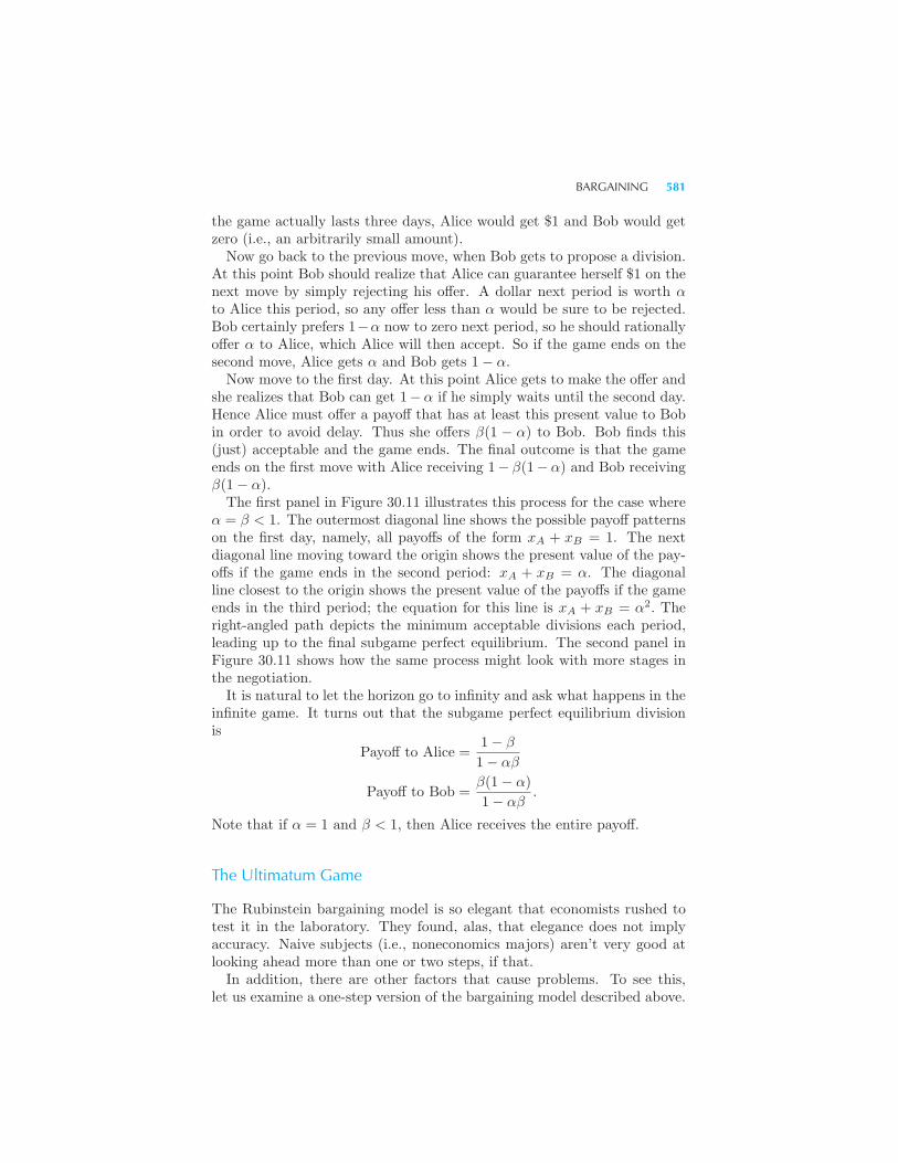
BARGAINING 581
the game actually lasts three days, Alice would get $1 and Bob would getzero (i.e., an arbitrarily small amount).Now go back to the previous move, when Bob gets to propose a division.
At this point Bob should realize that Alice can guarantee herself $1 on thenext move by simply rejecting his offer. A dollar next period is worth αto Alice this period, so any offer less than α would be sure to be rejected.Bob certainly prefers 1−α now to zero next period, so he should rationallyoffer α to Alice, which Alice will then accept. So if the game ends on thesecond move, Alice gets α and Bob gets 1− α.Now move to the first day. At this point Alice gets to make the offer and
she realizes that Bob can get 1−α if he simply waits until the second day.Hence Alice must offer a payoff that has at least this present value to Bobin order to avoid delay. Thus she offers β(1 − α) to Bob. Bob finds this(just) acceptable and the game ends. The final outcome is that the gameends on the first move with Alice receiving 1− β(1−α) and Bob receivingβ(1− α).The first panel in Figure 30.11 illustrates this process for the case where
α = β < 1. The outermost diagonal line shows the possible payoff patternson the first day, namely, all payoffs of the form xA + xB = 1. The nextdiagonal line moving toward the origin shows the present value of the pay-offs if the game ends in the second period: xA + xB = α. The diagonalline closest to the origin shows the present value of the payoffs if the gameends in the third period; the equation for this line is xA + xB = α2. Theright-angled path depicts the minimum acceptable divisions each period,leading up to the final subgame perfect equilibrium. The second panel inFigure 30.11 shows how the same process might look with more stages inthe negotiation.It is natural to let the horizon go to infinity and ask what happens in the
infinite game. It turns out that the subgame perfect equilibrium divisionis
Payoff to Alice =1− β
1− αβ
Payoff to Bob =β(1− α)
1− αβ.
Note that if α = 1 and β < 1, then Alice receives the entire payoff.
The Ultimatum Game
The Rubinstein bargaining model is so elegant that economists rushed totest it in the laboratory. They found, alas, that elegance does not implyaccuracy. Naive subjects (i.e., noneconomics majors) aren’t very good atlooking ahead more than one or two steps, if that.In addition, there are other factors that cause problems. To see this,
let us examine a one-step version of the bargaining model described above.
582 GAME APPLICATIONS (Ch. 30)
BOB’SPAYOFF
BOB’SPAYOFF
ALICE’S PAYOFF
ALICE’S PAYOFF
Subgame perfectequilibrium Subgame perfect
equilibrium
Day 3
a
a2
1
Day 2 Day 1
Figure30.11
A bargaining game. The heavy line connects together theequilibrium outcomes in the subgames. The point on the linethat is furthest out is the subgame perfect equilibrium.
Alice and Bob still have $1 to divide between them. Alice proposes adivision, and, if Bob agrees, the game ends. The question is, what shouldAlice say?
According to the theory, she should propose something like 99 cents forAlice, 1 cent for Bob. Bob, figuring that 1 cent is better than nothing,accepts, and Alice goes home happy that she studied economics.
Unfortunately, it doesn’t work out like that. A more likely outcome isthat Bob, disgusted by the paltry 1 cent, says “No way,” and Alice endsup with nothing. Alice, recognizing this possibility, will tend to sweetenthe offer. In actual experiments, the average offer for U.S. undergraduatesis about 45 cents, and this offer tends to be accepted most of the time.
The offering players are behaving rationally, in the sense that the 45 centoffer is pretty close to maximizing the expected payoff, given the observedfrequency of rejection. It is the receiving players who behave differentlythan the theory predicts, since they reject small offers, even though thismakes them worse off.
There are many proposed explanations for this. One view is that toosmall an offer violates social norms of behavior. Indeed, economists havefound quite significant cross-cultural differences in behavior in ultimatumgames. Another, not inconsistent view, is that receivers get some utilitypayoff from hurting the offerers, in retaliation for the small offer. After all,if all you are losing is a penny, the satisfaction of striking back at the otherplayer is pretty attractive by comparison. We will the ultimatum game inmore detail in the next chapter.

REVIEW QUESTIONS 583
Summary
1. A player’s best response function gives the optimal choice for him as afunction of the choices the other player(s) might make.
2. A Nash equilibrium in a two-person game is a pair of strategies, one foreach player, each of which is a best response to the other.
3. A mixed strategy Nash equilibrium involves randomizing among severalstrategies.
4. Common games of coordination are the battle of the sexes, where bothplayers want to do the same thing rather than different things; the pris-oner’s dilemma, where the dominant strategy ends up hurting both players;the assurance game, where both players want to cooperate as long as theythink the other will cooperate; and chicken, where players want to avoiddoing the same thing.
5. A two-person zero-sum game is one where the payoffs to one player arethe negative of the payoffs to the other.
6. Evolutionary games are concerned with outcomes that are stable underpopulation reproduction.
7. In sequential games, players move in turn. Each player therefore has toreason about what the other will do in response to his or her choices.
8. In many sequential games, commitment is an important issue. Findingways to force commitment to play particular strategies can be important.
REVIEW QUESTIONS
1. In a two-person Nash equilibrium, each player is making a best responseto what? In a dominant strategy equilibrium, each player is making a bestresponse to what?
2. Look at the best responses for row and column in the section on mixedstrategies. Do these give rise to best response functions?
3. If both players make the same choice in a coordination game, all will bewell.
4. The text claims that row scores 62 percent of the time in equilibrium.Where does this number come from?

584 GAME APPLICATIONS (Ch. 30)
5. A contractor says that he intends to “low-ball the bid and make up forit on change orders.” What does he mean?
CHAPTER 31
BEHAVIORALECONOMICS
The economic model of consumer choice that we have studied is simpleand elegant, and is a reasonable starting place for many sorts of analy-sis. However, it is most definitely not the whole story, and in many casesa deeper model of consumer behavior is necessary to accurately describechoice behavior.The field of behavioral economics is devoted to studying how con-
sumers actually make choices. It uses some of the insights from psychologyto develop predictions about choices people will make and many of thesepredictions are at odds with the conventional economic model of “rational”consumers.In this chapter we will look at some of the most important phenomena
that have been identified by behavioral economists, and contrast the pre-dictions of these behavioral theories with those presented earlier in thisbook.1
1 In writing this chapter, I have found Colin F. Camerer, George Loewenstein, andMatthew Rabin’s book Advances in Behavioral Economics, Princeton UniversityPress, 2003, to be very useful, particularly the introductory survey by Camerer andLoewenstein. Other works will be noted as the relevant topics are discussed.
586 BEHAVIORAL ECONOMICS (Ch. 31)
31.1 Framing Effects in Consumer Choice
In the basic model of consumer behavior, the choices were described in theabstract: red pencils or blue pencils, hamburgers and french fries, and soon. However, in real life, people are strongly affected by how choices arepresented to them or framed.A faded pair of jeans in a thrift shop may be perceived very differently
than the same jeans sold in an exclusive store. The decision to buy astock may feel quite different than the decision to sell a stock, even if bothtransactions end up with the same portfolio. A store might sell dozens ofcopies of a book priced at $29.95, whereas the same book priced at $29.00would have substantially fewer sales.These are all examples of framing effects, and they are clearly a pow-
erful force in choice behavior. Indeed, much of marketing practice is basedon understanding and utilizing such biases in consumer choice.
The Disease Dilemma
Framing effects are particularly common in choices involving uncertainty.For example, consider the following decision problem:2
A serious disease threatens 600 people. You are offered a choice betweentwo treatments, A and B, which will yield the following outcomes.
Treatment A. Saving 200 lives for certain.
Treatment B. A 1/3 chance of saving 600 lives and a 2/3 chance of savingno one.
Which would you choose? Now consider the choices between these treat-ments.
Treatment C. Having 400 people die for certain.
Treatment D. A 2/3 chance of 600 people dying and a 1/3 chance of noone dying.
Now which treatment would you choose?
2 A. Tversky and D. Kahneman, 1981, “The framing of decisions and the psychologyof choice,” Science, 211, 453–458.
FRAMING EFFECTS IN CONSUMER CHOICE 587
In the positive framing comparison—which describes how many peoplewill live—most individuals choose A over B, but in the negative framingcomparison most people choose D over C even though the outcomes in A-Cand B-D are exactly the same. Apparently, framing the question positively(in terms of lives saved) makes a treatment much more attractive thanframing the choice negatively (in terms of lives lost).Even expert decisions makers can fall into this trap. When psychologists
tried this question on a group of physicians, 72 percent of them chose thesafe treatment A over the risky treatment B. But when the question wasframed negatively, only 22 percent chose the risky treatment C while 72percent chose the safe treatment.Though few of us are faced with life-or-death decisions, there are similar
examples for more mundane choices, such as buying or selling stocks. Arational choice of an investment portfolio would, ideally, depend on anassessment of the possible outcomes of the investments rather than howone acquired those investments.For example, suppose that you are given 100 shares of stock in Concrete-
Blocks.com (whose slogan is “We give away the blocks, you pay for packingand shipping”). You might be reluctant to sell shares you received as a giftdespite the fact that you would never consider buying them yourself.People are often reluctant to sell losing stocks, thinking that they will
“come back.” Maybe they will, maybe they won’t. But ultimately youshouldn’t let history determine your investment portfolio—the right ques-tion to ask is whether you have the portfolio choices today that you want.
Anchoring Effects
The hypothetical ConcreteBlocks.com example described above is relatedto the so-called anchoring effect. The idea here is that people’s choicescan be influenced by completely spurious information. In a classic studythe experimenter spun a wheel of fortune and pointed out the number thatcame up to a subject.3 The subject was then asked whether the numberof African countries in the United Nations was greater or less than thenumber on the wheel of fortune.After they responded, the subjects were asked for their best guess about
how many African countries were in the United Nations. Even though thenumber shown on the wheel of fortune was obviously random, it exerted asignificant influence on the subjects’ reported guesses.In a similar experimental design, MBA students were given an expensive
bottle of wine and then asked if they would pay an amount for that bottleequal to the last two digits of their Social Security number. For example,
3 D. Kahneman and A. Tversky, 1974, “Judgment under uncertainty: Heuristics andbiases,” Science, 185: 1124–1131.
588 BEHAVIORAL ECONOMICS (Ch. 31)
if the last two digits were 29, the question was “Would you pay $29 for thisbottle of wine?”After answering that question, the students were asked what the maxi-
mum amount is that they were willing to pay for the wine. Their answersto this latter question were strongly influenced by the price determined bythe last two digits of their Social Security number. For example, those withSocial Security digits of 50 or under were willing to pay $11.62 on average,while those with digits in the upper half of the distribution were willing topay $19.95 on average.Again, these choices seem like mere laboratory games. However, there
are very serious economic decisions that can also be influenced by minorvariations in the way the choice is framed.Consider, for example, choices of pension plans.4
Some economists looked at data from three employers that offered au-tomatic enrollment in 401(k) plans. Employees could opt out, but theyhad to make an explicit choice to do so. The economists found that theparticipation rate in these programs with automatic enrollment was spec-tacularly high, with over 85 percent of workers accepting the default choiceof enrolling in the 401(k) plans.That’s the good news. The bad news is that almost all of these workers
also chose the default investment, typically a money market fund with verylow returns and a low monthly contribution. Presumably, the employersmade the default investment highly conservative to eliminate downside riskand possible employee lawsuits.In subsequent work, these economists examined the experience at a com-
pany where there was no default choice of pension plan: within a monthof starting work, employees were required to choose either to enroll in the401(k) plan or to postpone enrollment.By eliminating the standard default choices of non-enrollment, and of
enrollment in a fund that had low rates of return, this “active decision”approach raised participation rates from 35 percent to 70 percent for newlyhired employees. Moreover, employees who enrolled in the 401(k) planoverwhelmingly chose high savings rates.As this example illustrates, careful design of human resources benefits
programs can make a striking difference in which programs are chosen,potentially having a large effect on consumer savings behavior.
Bracketing
People often have trouble understanding their own behavior, finding it toodifficult to predict what they will actually choose in different circumstances.
4 James Choi, David Laibson, Brigitte Madrian, and Andrew Metrick, “For Betteror for Worse: Default Effects and 401(k) Savings Behavior,” NBER working paper,W8651, 2001.
FRAMING EFFECTS IN CONSUMER CHOICE 589
For example, a marketing professor gave students a choice of six differentsnacks that they could consume in each of three successive weeks duringclass.5 (You should be so lucky!) In one treatment, the students had tochoose the snacks in advance; in the other treatment, they chose the snackson each day then immediately consumed them.When the students had to choose in advance, they chose a much more
diverse set of snacks. In fact, 64 percent chose a different snack each week inthis treatment compared to only 9 percent in the other group. When facedwith making the choices all at once, people apparently preferred varietyto exclusivity. But when it came down to actually choosing, they madethe choice with which they were most comfortable. We are all creatures ofhabit, even in our choice of snacks.
Too Much Choice
Conventional theory argues that more choice is better. However, this claimignores the costs of making choices. In affluent countries, consumers caneasily become overwhelmed with choices, making it difficult for them toarrive at a decision.In one experiment, two marketing researchers set up sampling booths
for jam in a supermarket.6 One booth offered 24 flavors and one offeredonly 6. More people stopped at the larger display, but substantially morepeople actually bought jam at the smaller display. More choice seemed tobe attractive to shoppers, but the profusion of choices in the larger displayappeared to make it more difficult for the shoppers to reach a decision.Two experts in behavioral finance wondered whether the same problem
with “excessive choice” showed up in investor decisions. They found thatpeople who designed their own retirement portfolios tended to be just ashappy with the average portfolio chosen by their co-workers as they werewith their own choice. Having the flexibility to construct their own retire-ment portfolios didn’t seem to make investors feel better off.7
Constructed Preferences
How are we to interpret these examples? Psychologists and behavioraleconomists argue that preferences are not a guide to choice; rather, prefer-ences are “discovered” in part through the experiences of choice.
5 I. Simonson, 1990, “The effect of purchase quantity and timing on variety-seekingbehavior,” Journal of Marketing Research, 17: 150–164.
6 Sheena S. Iyengar and Mark R. Lepper, “When choice is demotivating: can one desiretoo much of a good thing?” Journal of Personality and Social Psychology, 2000.
7 Shlomo Benartzi and Richard Thaler, “How Much Is Investor Autonomy Worth?”UCLA working paper, 2001.
590 BEHAVIORAL ECONOMICS (Ch. 31)
Imagine watching someone in the supermarket picking up a tomato,putting it down, then picking it up again. Do they want it or not? Isthe price-quality combination offered acceptable? When you watch suchbehavior, you are seeing someone who is “on the margin” in terms of mak-ing the choice. They are, in the psychologists’ interpretation, discoveringtheir preferences.Conventional theory treats preferences as preexisting. In this view, pref-
erences explain behavior. Psychologists instead think of preferences asbeing constructed—people develop or create preferences through the act ofchoosing and consuming.It seems likely that the psychological model is a better description of what
actually happens. However, the two viewpoints are not entirely incompat-ible. As we have seen, once preferences have been discovered, albeit bysome mysterious process, they tend to become built-in to choices. Choices,once made, tend to anchor decisions. If you tried to buy that tomato fromthat consumer once they have finally decided to choose it, you would likelyhave to pay more than it cost them.
31.2 Uncertainty
Ordinary choice is complicated enough, but choice under uncertainty tendsto be particularly tricky. We’ve already seen that people’s decisions maydepend on how choice alternatives are phrased. But there are many otherbiases in behavior in this domain.
Law of Small Numbers
If you have taken a course in statistics, you might be familiar with the Lawof Large Numbers. This is a mathematical principle that says (roughly)that the average of a large sample from a population tends to be close tothe mean of that population.The Law of Small Numbers is a psychological statement that says that
people tend to be overly influenced by small samples, particularly if theyexperience them themselves.8
Consider the following question:9
8 The term originated with A. Tversky and D. Kahneman, 1971, “Belief in the law ofsmall numbers,” Psychological Bulletin,76, 2: 105–110. Much of the following discus-sion is based on a working paper by Matthew Rabin of the University of Californiaat Berkeley entitled “Inference by Believers in the Law of Small Numbers.”
9 A. Tversky and D. Kahneman, 1982, “Judgments of and by Representativeness,” inJudgment under Uncertainty: Heuristics and Biases, D. Kahneman, P. Slovic, andA. Tversky, Cambridge University Press, 84–98.
UNCERTAINTY 591
“A certain town is served by two hospitals. In the larger hospital about45 babies are born each day, and in the smaller hospital about 15 babiesare born each day. As you know, about 50 percent of all babies are boys.However, the exact percentage varies from day to day. Sometimes it maybe higher than 50 percent, sometimes lower. For a period of 1 year, eachhospital recorded the days on which more than 60 percent of the babiesborn were boys. Which hospital do you think recorded more such days?”
In a survey of college students, 22 percent of the subjects said that theythought that it was more likely that the larger hospital recorded more suchdays, while 56 percent said that they thought the number of days would beabout the same. Only 22 percent correctly said that the smaller hospitalwould report more days.If the correct account seems peculiar to you, suppose the smaller hospi-
tal recorded 2 births per day and the larger hospital 100 births per day.Roughly 25 percent of the time the smaller hospital would have 100 percentmale births, while this would be very rare for the large hospital.It appears that people expect samples to look like the distribution from
which they are drawn. Or, saying this another way, people underestimatethe actual magnitude of the fluctuations in a sample.A related issue is that people find it difficult to recognize randomness. In
one experiment, subjects were asked to write down a series of 150 “random”coin tosses. About 15 percent of the sequences they produced had headsor tails three times in a row, but this pattern would occur randomly about25 percent of the time. Only 3 percent of the subjects’ sequences had 4heads or 4 tails in a row, while probability theory says that this shouldoccur about 12 percent of the time.This has important implications for game theory, for example. We saw
that in many cases people should try to randomize their strategy choicesso as to keep their opponents guessing. But, as the psychological literatureshows, people aren’t very good at randomizing. On the other hand, peoplearen’t very good at detecting non-random behavior either, at least withoutsome training in statistics. The point of mixed strategy equilibria is notthat choices are mathematically unpredictable, but rather that they shouldbe unpredictable by the players in the game.Some economic researchers studied final and semi-final tennis matches at
Wimbledon.10 Ideally, tennis players should switch their serves from sideto side so that their opponent can’t guess which side the serve is comingfrom. However, even very accomplished players can’t do this quite as wellas one might expect. According to the authors:
“Our tests indicate that the tennis players are not quite playing ran-
10 M. Walker and J. Wooders, 1999, “Minimax Play at Wimbledon,” University of Ari-zona working paper.
592 BEHAVIORAL ECONOMICS (Ch. 31)
domly: they switch their serves from left to right and vice versa somewhattoo often to be consistent with random play. This is consistent with ex-tensive experimental research in psychology and economics which indicatesthat people who are attempting to behave truly randomly tend to “switchtoo often.”
Asset Integration and Loss Aversion
In our study of expected utility we made an implicit assumption that whatindividuals cared about was the total amount of wealth that they endedup with in various outcomes. This is known as the asset integrationhypothesis.
Even though most people would accept this as a reasonable thing to do,it is hard to put into practice (even for economists). In general, peopletend to avoid too many small risks and accept too many large risks.Suppose that you make $100,000 a year and that you are offered a coin
flip. If heads comes up you get $14 and if tails comes up you lose $10. Thisbet has an expected value of $12 and has a minuscule effect on your totalincome in a given year. Unless you have moral scruples about gambling,this would be a very attractive bet and you should almost certainly takeit. However, a surprisingly large number of people won’t take such a bet.This excess risk aversion shows up in insurance markets where people
tend to over-insure themselves against various small events. For example,people buy insurance against loosing their cell phone, even though theycan often replace it at quite a low cost. People also buy auto insurancewith deductibles that are much too low to make economic sense.In general, when making insurance decisions you should look at the
“house odds.” If cell phone insurance costs you $3 a month, or $36 ayear, and a new cell phone costs $180, then the house odds are 36/180,or 20 percent. The cell phone insurance would pay off in expected valueonly if you have more than a 20 percent chance of losing your phone or ifit would be an extreme financial hardship to replace it.It appears that people aren’t really risk averse as much as they are
loss averse. That is, people put seemingly excessive weight on the statusquo—where they start—as opposed to where they end up.In an experiment that has been replicated many times, two researchers
gave half of the subjects in a group coffee mugs.11 They asked this group toreport the lowest price at which they would sell the mugs. Then they askedthe group that didn’t have mugs the highest price at which they would buya mug. Since the groups were chosen randomly, the buying and sellingprices should be about equal. However, in the experiment, the median
11 D. Kahneman, J. L. Kitsch, and R. Thaler, 1990, “Experimental tests of the endow-ment effect and the Coase theorem,” Journal of Political Economy, 98, 1325–1348.
TIME 593
selling price was $5.79 and the median buying price was $2.25, a substantialdifference. Apparently, the subjects with coffee mugs were more reluctantto part with them than subjects without mugs. Their preferences seemed tobe influenced by their endowment, contrary to standard consumer theory.A similar effect shows up in what is known as the sunk cost fallacy.
Once you have bought something, the amount you paid is “sunk,” or nolonger recoverable. So future behavior should not be influenced by sunkcosts.But, alas, real people tend to care about how much they paid for some-
thing. Researchers have found that the price at which owners listed con-dominiums in Boston was highly correlated with the buying price.12 Aspointed out earlier, owners of stock are very reluctant to realize losses, evenwhen it would be advantageous for tax reasons.The fact that ordinary people are subject to the sunk cost fallacy is in-
teresting, but perhaps it is even more interesting that professionals are lesssusceptible to this problem. For example, the authors of the condominiumexample mentioned above found that individuals who bought condos forinvestment purposes were less likely to be influenced by sunk costs thanindividuals who lived in the condos.Similarly, financial advisers are seldom reluctant to realize losses, partic-
ularly when there is a tax advantage to do so. It appears that one reasonto hire professional advisers is to draw on their dispassionate analysis ofdecisions.
31.3 Time
Just as behavior involving uncertainty is subject to various forms of anoma-lous behavior, behavior involving time has its own set of anomalies.
Discounting
Consider, for example, time discounting. A standard model in economics,exponential discounting, posits that people discount the future at aconstant fraction. If u(c) is the utility of consumption today, then theutility of consumption t years in the future looks like δtu(c), where δ < 1.
This is a mathematically convenient specification, but there are otherforms of discounting that seem to fit the data better.One economist auctioned off bonds that paid off at various times in the
future and found that people valued payment at future times less than the
12 David Genesove and Christopher Mayer, 2001, “Loss aversion and seller behavior:Evidence from the housing market,” Quarterly Journal of Economics, 116, 4, 1233–1260.
594 BEHAVIORAL ECONOMICS (Ch. 31)
exponential discounting theory would predict. An alternative theory, calledhyperbolic discounting, suggests that the discount factor does not takethe form δt but rather takes the form 1/(1 + kt).
One particularly attractive feature of exponential discounting is thatbehavior is “time consistent.” Think about a person with a three-periodplanning horizon with utility function of the form
u(c1) + δu(c2) + δ2u(c3).
The marginal rate of substitution between periods 1 and 2 is
MRS12 =δMU(c2)
MU(c1),
while the MRS between periods 2 and 3 is
MRS23 =δ2MU(c3)
δMU(c2)=
δMU(c3)
MU(c2).
This last expression shows that the rate at which the individual is will-ing to substitute consumption in period 2 for consumption in period 3 isthe same whether viewed from the perspective of period 1 or of period 2.This is not true for hyperbolic discounting. An individual with hyperbolicdiscounting discounts the long-term future more heavily than he discountsthe short-term future.Such a person will exhibit time inconsistency: he may make a plan
today about his future behavior, but when the future arrives he will wantto do something different. Think of a couple who decide to spend $5,000on a trip to Europe rather than save their money. They rationalize theirdecision on the grounds that they will start saving next summer. But whennext summer arrives, they decide to spend their money on a cruise.
Self-control
A closely related issue to the time consistency problem is the problem ofself-control. Almost everyone faces this issue to some degree. We mightvow to count our calories and eat less while standing on the bathroomscale, but our resolve can easily vanish when we sit down to a nice meal.Rational people are apparently slim and healthy, unlike the rest of us.One important question is whether people are aware of their own diffi-
culties with self-control. If I know that I have a tendency to procrastinate,perhaps I should realize that when an important task comes along I shoulddo it right away. Or if I have a tendency to overcommit myself, perhaps Ishould learn to say no more often.
STRATEGIC INTERACTION AND SOCIAL NORMS 595
But there is the other possibility. If I know that I am likely to yieldto the temptation to have another desert tomorrow, I may as well haveanother desert today. The flesh is weak, but the spirit may be weak too.One way to deal with self-control is to find ways to commit yourself to
future actions. That is, you can try to find a way to make it more costlyto deviate from the desired action in the future. For example, peoplewho make a public pronouncement about their future behavior might beless likely to deviate from their intended behavior. There are pills foralcoholics that make them violently sick if they drink alcohol. There arealso commitment devices for dieters: someone who has his stomachstapled will be less likely to overeat.Contracts between individuals are there to ensure that people carry out
their future intentions—even when it might not be attractive for them todo so due to changed conditions. In a similar way, people can hire othersto impose costs on them if they deviate from intended actions, making, ineffect, a contract with themselves. Dieting spas, exercise instructors, andtutors are forms of “purchased self-control.”
EXAMPLE: Overconfidence
An interesting variation on self-control is the phenomenon of overconfi-dence. Two financial economists, Brad Barber and Terrance Odean, stud-ied the performance of 66,465 households with discount brokerage accounts.During the period they studied, households that traded infrequently re-ceived an 18 percent return on their investments, while the return for thehouseholds that traded most actively was 11.3 percent.One of the most important factors that apparently influenced this exces-
sive trading was gender: the men traded a lot more than women. Psychol-ogists commonly find that men tend to have excessive confidence in theirown abilities, while women, for the most part, tend to be more realistic.Psychologists refer to men’s behavior as self-serving attribution bias. Basi-cally, men (or at least some men) tend to think their successes are a resultof their own skill, rather than dumb luck, and so become overconfident.This overconfidence can have financial repercussions. In the sample of
brokerage accounts, men traded 45 percent more than women. This exces-sive trading resulted in the average return to men that was a full percentagepoint lower than the return to women. As Barber and Odean put it, “trad-ing can be hazardous to your wealth.”
31.4 Strategic Interaction and Social Norms
A particularly interesting set of psychological, or perhaps sociological, be-haviors arise in strategic interaction. We have studied game theory, which
596 BEHAVIORAL ECONOMICS (Ch. 31)
attempts to predict how rational players should interact. But there is alsoa subject known as behavioral game theory that examines how actualpeople interact. Indeed, there are systematic and strong deviations fromthe pure theory.
Ultimatum Game
Consider the ultimatum game, which was discussed briefly in the lastchapter. As you will recall, this is a game with two players, the proposerand the responder. The proposer is given $10 and asked to propose adivision between himself and the responder. The responder is then shownthe division and asked whether or not he wishes to accept it. If he accepts,the division is carried out; if he refuses the division, both people walk awaywith nothing.Let’s first think about how fully rational players might act. Once the
responder sees the division, he has a dominant strategy: accept the moneyas long as he gets anything at all. After all, suppose I offer you the choicebetween 10 cents and nothing. Wouldn’t you rather have 10 cents thannothing at all?Given that a rational responder will choose any amount, the divider
should choose the minimal amount to give him—say, a penny. So theoutcome predicted by game theory is an extreme split: the divider will endup with almost everything.This isn’t the way things turn out when the game is actually played. In
fact, responders tend to reject offers that they perceive as unfair. Offersthat give the responder less than 30 percent of the amount to be dividedare rejected more than 50 percent of the time.Of course, if the divider recognizes that the responder will reject “unfair”
offers, the divider will rationally want to make a division that is closer toequal. The average division tends to be about 45 percent to the responderand 55 percent to the divider, with about 16 percent of the offers beingrejected.There has been a considerable amount of literature examining how the
characteristics of the players affect the outcome of the game. One exampleis gender differences: it appears that men tend to receive more favorabledivisions, particularly when the divisions are made by women.Cultural differences can also be important. It appears that some cul-
tures value fairness more than others, inducing people to reject offers thatare perceived as unfair.13 Interestingly enough, the offered amounts don’tvary much from region to region and culture to culture, while there are
13 See Swee-Hoon Chuah, Robert Hoffman, Martin Jones, and Geoffrey Williams, “DoCultures Clash? Evidence from Cross-National Ultimatum Game Experiments,” Not-tingham University Business School working paper.
ASSESSMENT OF BEHAVIORAL ECONOMICS 597
systematic differences in the divisions that are acceptable. The size of thepie is also important. If the size of the pie is $10, you might be reluctantto accept $1. But if the size of the pie is $1,000, would you be willing toreject $100? Apparently, responders do find it difficult to turn down largeramounts of money.Another variation is in the design of the game. In one variant, the so-
called strategy method, the responders are asked to name the minimaldivision that they will accept before seeing the amount they are offered. Theproposers are aware that the decision will be made in advance but, of course,don’t know what the minimum acceptable division is. This experimentaldesign tends to increase the amounts that the proposers offer; that is, ittends to make the divisions more equal.
Fairness
One effect at work in the ultimatum game seems to be a concern for fairness.Most people seem to have a natural bias towards equal (or at least not toounequal) division. This is not simply an individual phenomenon, but asocial phenomenon. People will enforce fairness norms even when it isnot directly in their interest to do so.Consider, for example, punishment games, which are a generalization
of ultimatum games with a third party who observes the choices made bythe proposer/divider. The third party can choose, at some cost to himself,to deduct some of the proposer’s profits.14
Experimenters have found that around 60 percent of these third-partyobservers will actually punish those who make unfair divisions. There seemsto be something in the human makeup—whether innate or learned—thatfinds unfair behavior objectionable.Indeed, there are differences across cultures with respect to social norms
for fairness; individuals in some societies seem to value it highly, while inother societies fairness is less strongly valued. However, the urge to punishthose who are unfair is widely felt. It has been suggested that a predilec-tion towards “fair” outcomes is part of human nature, perhaps becauseindividuals that behaved fairly towards each other had higher chances ofsurviving and reproducing.
31.5 Assessment of Behavioral Economics
Psychologists, marketers, and behavioral economists have amassed a vari-ety of examples showing how the basic theory of economic choice is wrong,or, at least, incomplete.
14 See Ernst Fehr and Urs Fischbacher, 2004, “Third-party punishment and socialnorms,” Evolution and Human Behavior, 25, 63–87.
598 BEHAVIORAL ECONOMICS (Ch. 31)
Some of these examples appear to be “optical illusions.” For example,the fact that framing a choice problem differently can affect decisions issimilar to the fact that human judgment of sizes and distances can beaffected by how figures are drawn. If people took the time to consider thechoices carefully—applying a measuring stick of dispassionate reasoning—they would reach the right conclusion.Though it is undoubtedly true that people don’t behave completely in
accord with the simplest theories of economic behavior, one still mightrespond that no theory is 100 percent correct. Psychologists have also doc-umented that people don’t really understand simple principles of physics.Example: If you tie a weight to the end of a rope, swing it around yourhead in a circle and then let go, which way will the weight fly?Many people say that the weight will fly radially outward rather than
the correct response that the weight will move tangentially to the circle.15
Of course, people have lived in the physical world their entire lives. If theyoccasionally misunderstand how it works, we shouldn’t be too surprisedwhen people misunderstand the economic world.Apparently our intuitive understanding of physics is good enough for
everyday life, and even the demands of amateur and professional sports: abaseball player may not be able to describe how a ball will travel, despitethe fact that he can throw it well. Similarly, one might argue that peopletend to be pretty good at the sorts of day-to-day decisions they are forcedto make, even if they aren’t very good at abstract reasoning about them.Another reaction to behavioral anomalies is that markets tend to reward
rational behavior, while punishing irrationality. Even if many participantsdo not behave rationally, those who do behave sensibly will have the biggesteffect on prices and outcomes. There is likely some truth to this viewas well. Recall the example that real estate investors seemed to be lessinfluenced by sunk costs than ordinary individuals.In addition, you can hire experts to help you make better decisions. Diet
consultants and financial advisers can offer objective advice about how toeat and how to invest. If you are worried about being too fair, you canalways hire a tough negotiator.Returning to the optical illusion example, the reason that we use rulers
and yardsticks is that we learn not to trust our own eyes. Similarly, inmaking important decisions it is prudent to consult the views of objectiveexperts.
15 See M. McCloskey, 1983, “Intuitive Physics,” Scientific American, April, 114–123.
REVIEW QUESTIONS 599
Summary
1. Behavioral economics is concerned with how consumers make choices inreality.
2. In many cases, actual consumer behavior is different from that predictedby the simple model of the rational consumer.
3. Consumers make different choices depending on how a problem is framedor presented.
4. The default matters a lot.
5. People find it difficult to predict their own choice behavior.
6. Too many choices may be overwhelming and make it difficult to make adecision.
7. Choice behavior can be particularly problematic in choices involvinguncertainty.
8. Peole tend to exhibit excess risk aversion in experimental settings.
9. People may discount the future more heavily than conventional theoryassumes.
10. Time inconsistency means that actual choices may end up being dif-ferent than planned choices.
11. The ultimatum game involves one player proposing a division of somemoney and the other player either accepting that division or ending thegame. Conventional game theory predicts very unfairm divisions.
12. However, consumers seem to have a preference for “fair” divisions andwill punish those who behave unfairly, even if harms themselves.
REVIEW QUESTIONS
1. Subjects are allowed to buy tickets in a lottery. One group is told thatthey have a 55 percent chance of winning, the other group is told that theyhave a 45 percent chance of not winning. Which group is more likely tobuy lottery tickets? What is the name for this effect?
600 BEHAVIORAL ECONOMICS (Ch. 31)
2. Mary plans the entire week’s meals for her family, while Fred shops eachday. Which is likely to produce more varied meals? What is this effectcalled?
3. You are the human resources director for a medium-size company andare trying to decide how many mutual funds to offer in your employees’pension plan. Would it be better to offer 10 choices or 50 choices?
4. What is the probability that a fair coin will come up heads three timesin a row when tossed?
5. John decides that he will save $5 this week and $10 next week. Butwhen next week arrives, he decides to save only $8. What is the term usedto describe this sort of inconsistent behavior?

CHAPTER 32
EXCHANGE
Up until now we have generally considered the market for a single good inisolation. We have viewed the demand and supply functions for a good asdepending on its price alone, disregarding the prices of other goods. But ingeneral the prices of other goods will affect people’s demands and suppliesfor a particular good. Certainly the prices of substitutes and complementsfor a good will influence the demand for it, and, more subtly, the pricesof goods that people sell will affect the amount of income they have andthereby influence how much of other goods they will be able to buy.Up until now we have been ignoring the effect of these other prices on
the market equilibrium. When we discussed the equilibrium conditions in aparticular market, we only looked at part of the problem: how demand andsupply were affected by the price of the particular good we were examining.This is called partial equilibrium analysis.In this chapter we will begin our study of general equilibrium analysis:
how demand and supply conditions interact in several markets to determinethe prices of many goods. As you might suspect, this is a complex problem,and we will have to adopt several simplifications in order to deal with it.First, we will limit our discussion to the behavior of competitive markets,
so that each consumer or producer will take prices as given and optimize
602 EXCHANGE (Ch. 32)
accordingly. The study of general equilibrium with imperfect competitionis very interesting but too difficult to examine at this point.Second, we will adopt our usual simplifying assumption of looking at the
smallest number of goods and consumers that we possibly can. In this case,it turns out that many interesting phenomena can be depicted using onlytwo goods and two consumers. All of the aspects of general equilibriumanalysis that we will discuss can be generalized to arbitrary numbers ofconsumers and goods, but the exposition is simpler with two of each.Third, we will look at the general equilibrium problem in two stages.
We will start with an economy where people have fixed endowments ofgoods and examine how they might trade these goods among themselves;no production will be involved. This case is naturally known as the caseof pure exchange. Once we have a clear understanding of pure exchangemarkets we will examine production behavior in the general equilibriummodel.
32.1 The Edgeworth Box
There is a convenient graphical tool known as the Edgeworth box thatcan be used to analyze the exchange of two goods between two people.1 TheEdgeworth box allows us to depict the endowments and preferences of twoindividuals in one convenient diagram, which can be used to study variousoutcomes of the trading process. In order to understand the constructionof an Edgeworth box it is necessary to examine the indifference curves andthe endowments of the people involved.Let us call the two people involved A and B and the two goods involved
1 and 2. We will denote A’s consumption bundle by XA = (x1A, x
2A), where
x1A represents A’s consumption of good 1 and x2
A represents A’s consump-tion of good 2. Then B’s consumption bundle is denoted byXB = (x1
B , x2B).
A pair of consumption bundles, XA and XB , is called an allocation. Anallocation is a feasible allocation if the total amount of each good con-sumed is equal to the total amount available:
x1A + x1
B = ω1A + ω1
B
x2A + x2
B = ω2A + ω2
B .
A particular feasible allocation that is of interest is the initial endow-ment allocation, (ω1
A, ω2A) and (ω1
B , ω2B). This is the allocation that the
consumers start with. It consists of the amount of each good that con-sumers bring to the market. They will exchange some of these goods witheach other in the course of trade to end up at a final allocation.
1 The Edgeworth box is named in honor of Francis Ysidro Edgeworth (1845–1926), anEnglish economist who was one of the first to use this analytical tool.
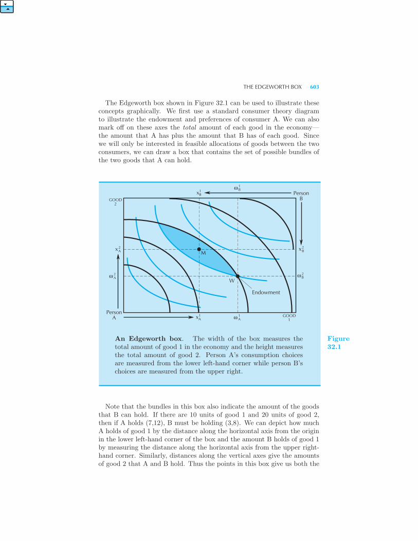
THE EDGEWORTH BOX 603
The Edgeworth box shown in Figure 32.1 can be used to illustrate theseconcepts graphically. We first use a standard consumer theory diagramto illustrate the endowment and preferences of consumer A. We can alsomark off on these axes the total amount of each good in the economy—the amount that A has plus the amount that B has of each good. Sincewe will only be interested in feasible allocations of goods between the twoconsumers, we can draw a box that contains the set of possible bundles ofthe two goods that A can hold.
x1A
1Aω GOOD
1
2Ax
1Bx
2Bx
ω 2B
ω 1B
ω 2A
PersonA
M
Endowment
PersonBGOOD
2
W
An Edgeworth box. The width of the box measures thetotal amount of good 1 in the economy and the height measuresthe total amount of good 2. Person A’s consumption choicesare measured from the lower left-hand corner while person B’schoices are measured from the upper right.
Figure32.1
Note that the bundles in this box also indicate the amount of the goodsthat B can hold. If there are 10 units of good 1 and 20 units of good 2,then if A holds (7,12), B must be holding (3,8). We can depict how muchA holds of good 1 by the distance along the horizontal axis from the originin the lower left-hand corner of the box and the amount B holds of good 1by measuring the distance along the horizontal axis from the upper right-hand corner. Similarly, distances along the vertical axes give the amountsof good 2 that A and B hold. Thus the points in this box give us both the
604 EXCHANGE (Ch. 32)
bundles that A can hold and the bundles that B can hold—just measuredfrom different origins. The points in the Edgeworth box can represent allfeasible allocations in this simple economy.We can depict A’s indifference curves in the usual manner, but B’s indif-
ference curves take a somewhat different form. To construct them we takea standard diagram for B’s indifference curves, turn it upside down, and“overlay” it on the Edgeworth box. This gives us B’s indifference curveson the diagram. If we start at A’s origin in the lower left-hand corner andmove up and to the right, we will be moving to allocations that are morepreferred by A. As we move down and to the left we will be moving toallocations that are more preferred by B. (If you rotate your book and lookat the diagram, this discussion may seem clearer.)The Edgeworth box allows us to depict the possible consumption bundles
for both consumers—the feasible allocations—and the preferences of bothconsumers. It thereby gives a complete description of the economicallyrelevant characteristics of the two consumers.
32.2 Trade
Now that we have both sets of preferences and endowments depicted wecan begin to analyze the question of how trade takes place. We startat the original endowment of goods, denoted by the point W in Figure32.1. Consider the indifference curves of A and B that pass through thisallocation. The region where A is better off than at her endowment consistsof all the bundles above her indifference curve through W . The regionwhere B is better off than at his endowment consists of all the allocationsthat are above—from his point of view—his indifference curve through W .(This is below his indifference curve from our point of view . . . unless you’vestill got your book upside down.)Where is the region of the box where A and B are both made better
off? Clearly it is in the intersection of these two regions. This is the lens-shaped region illustrated in Figure 32.1. Presumably in the course of theirnegotiations the two people involved will find some mutually advantageoustrade—some trade that will move them to some point inside the lens-shapedarea such as the point M in Figure 32.1.The particular movement to M depicted in Figure 32.1 involves person
A giving up |x1A−ω1
A| units of good 1 and acquiring in exchange |x2A−ω2
A|units of good 2. This means that B acquires |x1
B −ω1B | units of good 1 and
gives up |x2B − ω2
B | units of good 2.There is nothing particularly special about the allocation M . Any allo-
cation inside the lens-shaped region would be possible—for every allocationof goods in this region is an allocation that makes each consumer better offthan he or she was at the original endowment. We only need to supposethat the consumers trade to some point in this region.
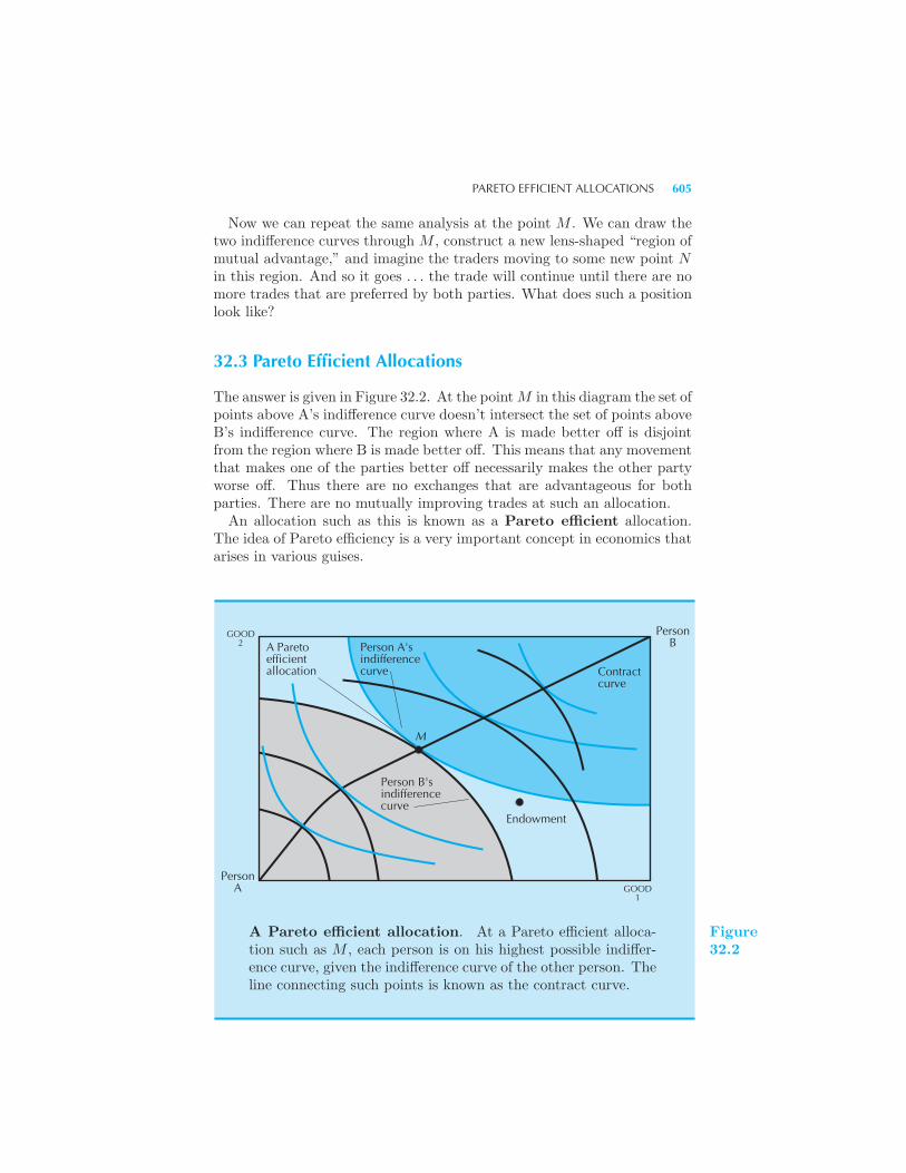
PARETO EFFICIENT ALLOCATIONS 605
Now we can repeat the same analysis at the point M . We can draw thetwo indifference curves through M , construct a new lens-shaped “region ofmutual advantage,” and imagine the traders moving to some new point Nin this region. And so it goes . . . the trade will continue until there are nomore trades that are preferred by both parties. What does such a positionlook like?
32.3 Pareto Efficient Allocations
The answer is given in Figure 32.2. At the pointM in this diagram the set ofpoints above A’s indifference curve doesn’t intersect the set of points aboveB’s indifference curve. The region where A is made better off is disjointfrom the region where B is made better off. This means that any movementthat makes one of the parties better off necessarily makes the other partyworse off. Thus there are no exchanges that are advantageous for bothparties. There are no mutually improving trades at such an allocation.An allocation such as this is known as a Pareto efficient allocation.
The idea of Pareto efficiency is a very important concept in economics thatarises in various guises.
Endowment
M
Person B'sindifferencecurve
Person A'sindifferencecurve
A Paretoefficientallocation Contract
curve
GOOD2
GOOD1
PersonB
PersonA
A Pareto efficient allocation. At a Pareto efficient alloca-tion such as M , each person is on his highest possible indiffer-ence curve, given the indifference curve of the other person. Theline connecting such points is known as the contract curve.
Figure32.2
606 EXCHANGE (Ch. 32)
A Pareto efficient allocation can be described as an allocation where:
1. There is no way to make all the people involved better off; or
2. there is no way to make some individual better off without makingsomeone else worse off; or
3. all of the gains from trade have been exhausted; or
4. there are no mutually advantageous trades to be made, and so on.
Indeed we have mentioned the concept of Pareto efficiency several timesalready in the context of a single market: we spoke of the Pareto efficientlevel of output in a single market as being that amount of output wherethe marginal willingness to buy equaled the marginal willingness to sell.At any level of output where these two numbers differed, there would be away to make both sides of the market better off by carrying out a trade.In this chapter we will examine more deeply the idea of Pareto efficiencyinvolving many goods and many traders.Note the following simple geometry of Pareto efficient allocations: the
indifference curves of the two agents must be tangent at any Pareto efficientallocation in the interior of the box. It is easy to see why. If the twoindifference curves are not tangent at an allocation in the interior of the box,then they must cross. But if they cross, then there must be some mutuallyadvantageous trade—so that point cannot be Pareto efficient. (It is possibleto have Pareto efficient allocations on the sides of the box—where oneconsumer has zero consumption of some good—in which the indifferencecurves are not tangent. These boundary cases are not important for thecurrent discussion.)From the tangency condition it is easy to see that there are a lot of Pareto
efficient allocations in the Edgeworth box. In fact, given any indifferencecurve for person A, for example, there is an easy way to find a Paretoefficient allocation. Simply move along A’s indifference curve until youfind the point that is the best point for B. This will be a Pareto efficientpoint, and thus both indifference curves must be tangent at this point.The set of all Pareto efficient points in the Edgeworth box is known as
the Pareto set, or the contract curve. The latter name comes fromthe idea that all “final contracts” for trade must lie on the Pareto set—otherwise they wouldn’t be final because there would be some improvementthat could be made!In a typical case the contract curve will stretch from A’s origin to B’s
origin across the Edgeworth box, as shown in Figure 32.2. If we start at A’sorigin, A has none of either good and B holds everything. This is Paretoefficient since the only way A can be made better off is to take somethingaway from B. As we move up the contract curve A is getting more andmore well-off until we finally get to B’s origin.
MARKET TRADE 607
The Pareto set describes all the possible outcomes of mutually advanta-geous trade from starting anywhere in the box. If we are given the startingpoint—the initial endowments for each consumer—we can look at the sub-set of the Pareto set that each consumer prefers to his initial endowment.This is simply the subset of the Pareto set that lies in the lens-shaped re-gion depicted in Figure 32.1. The allocations in this lens-shaped region arethe possible outcomes of mutual trade starting from the particular initialendowment depicted in that diagram. But the Pareto set itself doesn’tdepend on the initial endowment, except insofar as the endowment de-termines the total amounts of both goods that are available and therebydetermines the dimensions of the box.
32.4 Market Trade
The equilibrium of the trading process described above—the set of Paretoefficient allocations—is very important, but it still leaves a lot of ambiguityabout where the agents end up. The reason is that the trading process wehave described is very general. Essentially we have only assumed that thetwo parties will move to some allocation where they are both made betteroff.If we have a particular trading process, we will have a more precise
description of equilibrium. Let’s try to describe a trading process thatmimics the outcome of a competitive market.Suppose that we have a third party who is willing to act as an “auction-
eer” for the two agents A and B. The auctioneer chooses a price for good 1and a price for good 2 and presents these prices to the agents A and B.Each agent then sees how much his or her endowment is worth at the prices(p1, p2) and decides how much of each good he or she would want to buyat those prices.One warning is in order here. If there are really only two people involved
in the transaction, then it doesn’t make much sense for them to behave ina competitive manner. Instead they would probably attempt to bargainover the terms of trade. One way around this difficulty is to think of theEdgeworth box as depicting the average demands in an economy with onlytwo types of consumers, but with many consumers of each type. Anotherway to deal with this is to point out that the behavior is implausible inthe two-person case, but it makes perfect sense in the many-person case,which is what we are really concerned with.Either way, we know how to analyze the consumer-choice problem in this
framework—it is just the standard consumer-choice problem we describedin Chapter 5. In Figure 32.3 we illustrate the two demanded bundles ofthe two agents. (Note that the situation depicted in Figure 32.3 is not anequilibrium configuration since the demand by one agent is not equal tothe supply of the other agent.)
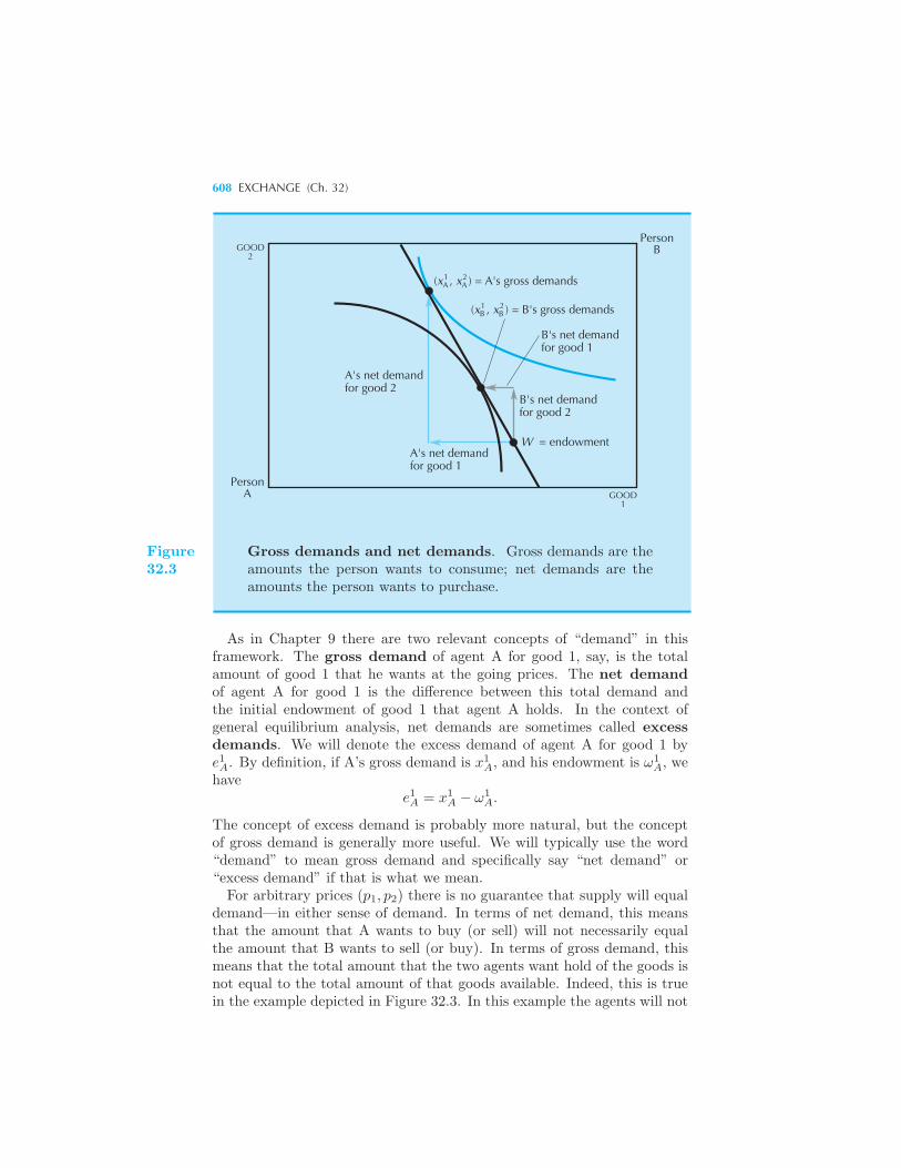
608 EXCHANGE (Ch. 32)
(x , x ) = A's gross demands1 2A A
A's net demandfor good 2
A's net demandfor good 1
B's net demandfor good 2
W = endowment
B's net demandfor good 1
PersonB
GOOD1
PersonA
GOOD2
B21
B(x , x ) = B's gross demands
Figure32.3
Gross demands and net demands. Gross demands are theamounts the person wants to consume; net demands are theamounts the person wants to purchase.
As in Chapter 9 there are two relevant concepts of “demand” in thisframework. The gross demand of agent A for good 1, say, is the totalamount of good 1 that he wants at the going prices. The net demandof agent A for good 1 is the difference between this total demand andthe initial endowment of good 1 that agent A holds. In the context ofgeneral equilibrium analysis, net demands are sometimes called excessdemands. We will denote the excess demand of agent A for good 1 bye1A. By definition, if A’s gross demand is x1
A, and his endowment is ω1A, we
havee1A = x1
A − ω1A.
The concept of excess demand is probably more natural, but the conceptof gross demand is generally more useful. We will typically use the word“demand” to mean gross demand and specifically say “net demand” or“excess demand” if that is what we mean.For arbitrary prices (p1, p2) there is no guarantee that supply will equal
demand—in either sense of demand. In terms of net demand, this meansthat the amount that A wants to buy (or sell) will not necessarily equalthe amount that B wants to sell (or buy). In terms of gross demand, thismeans that the total amount that the two agents want hold of the goods isnot equal to the total amount of that goods available. Indeed, this is truein the example depicted in Figure 32.3. In this example the agents will not
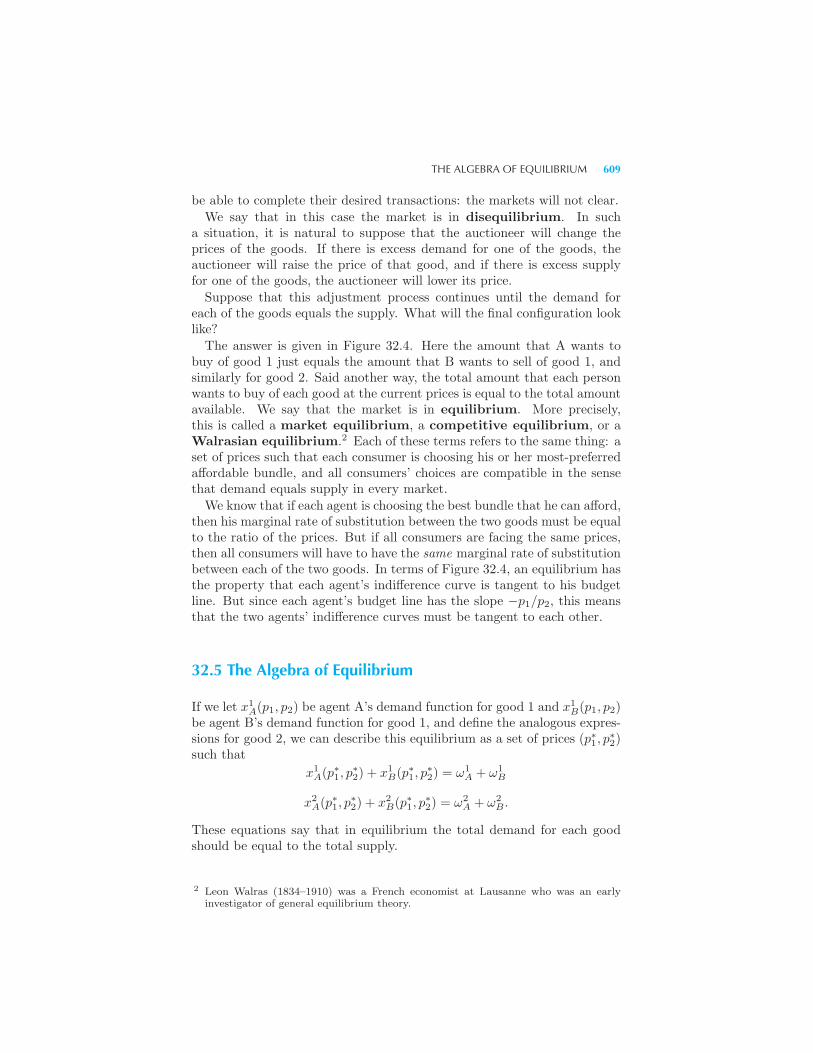
THE ALGEBRA OF EQUILIBRIUM 609
be able to complete their desired transactions: the markets will not clear.
We say that in this case the market is in disequilibrium. In sucha situation, it is natural to suppose that the auctioneer will change theprices of the goods. If there is excess demand for one of the goods, theauctioneer will raise the price of that good, and if there is excess supplyfor one of the goods, the auctioneer will lower its price.
Suppose that this adjustment process continues until the demand foreach of the goods equals the supply. What will the final configuration looklike?
The answer is given in Figure 32.4. Here the amount that A wants tobuy of good 1 just equals the amount that B wants to sell of good 1, andsimilarly for good 2. Said another way, the total amount that each personwants to buy of each good at the current prices is equal to the total amountavailable. We say that the market is in equilibrium. More precisely,this is called a market equilibrium, a competitive equilibrium, or aWalrasian equilibrium.2 Each of these terms refers to the same thing: aset of prices such that each consumer is choosing his or her most-preferredaffordable bundle, and all consumers’ choices are compatible in the sensethat demand equals supply in every market.
We know that if each agent is choosing the best bundle that he can afford,then his marginal rate of substitution between the two goods must be equalto the ratio of the prices. But if all consumers are facing the same prices,then all consumers will have to have the same marginal rate of substitutionbetween each of the two goods. In terms of Figure 32.4, an equilibrium hasthe property that each agent’s indifference curve is tangent to his budgetline. But since each agent’s budget line has the slope −p1/p2, this meansthat the two agents’ indifference curves must be tangent to each other.
32.5 The Algebra of Equilibrium
If we let x1A(p1, p2) be agent A’s demand function for good 1 and x1
B(p1, p2)be agent B’s demand function for good 1, and define the analogous expres-sions for good 2, we can describe this equilibrium as a set of prices (p∗1, p
∗2)
such that
x1A(p
∗1, p
∗2) + x1
B(p∗1, p
∗2) = ω1
A + ω1B
x2A(p
∗1, p
∗2) + x2
B(p∗1, p
∗2) = ω2
A + ω2B .
These equations say that in equilibrium the total demand for each goodshould be equal to the total supply.
2 Leon Walras (1834–1910) was a French economist at Lausanne who was an earlyinvestigator of general equilibrium theory.
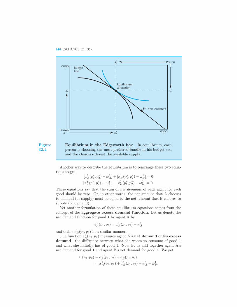
610 EXCHANGE (Ch. 32)
PersonB
xB1
B2x
W = endowment
Equilibriumallocation
Budgetline
GOOD2
Ax2
PersonA
1xAGOOD
1
Figure32.4
Equilibrium in the Edgeworth box. In equilibrium, eachperson is choosing the most-preferred bundle in his budget set,and the choices exhaust the available supply.
Another way to describe the equilibrium is to rearrange these two equa-tions to get
[x1A(p
∗1, p
∗2)− ω1
A] + [x1B(p
∗1, p
∗2)− ω1
B ] = 0
[x2A(p
∗1, p
∗2)− ω2
A] + [x2B(p
∗1, p
∗2)− ω2
B ] = 0.
These equations say that the sum of net demands of each agent for eachgood should be zero. Or, in other words, the net amount that A choosesto demand (or supply) must be equal to the net amount that B chooses tosupply (or demand).Yet another formulation of these equilibrium equations comes from the
concept of the aggregate excess demand function. Let us denote thenet demand function for good 1 by agent A by
e1A(p1, p2) = x1A(p1, p2)− ω1
A
and define e1B(p1, p2) in a similar manner.The function e1A(p1, p2) measures agent A’s net demand or his excess
demand—the difference between what she wants to consume of good 1and what she initially has of good 1. Now let us add together agent A’snet demand for good 1 and agent B’s net demand for good 1. We get
z1(p1, p2) = e1A(p1, p2) + e1B(p1, p2)
= x1A(p1, p2) + x1
B(p1, p2)− ω1A − ω1
B ,
WALRAS’ LAW 611
which we call the aggregate excess demand for good 1. There is asimilar aggregate excess demand for good 2, which we denote by z2(p1, p2).
Then we can describe an equilibrium (p∗1, p∗2) by saying that the aggregate
excess demand for each good is zero:
z1(p∗1, p
∗2) = 0
z2(p∗1, p
∗2) = 0.
Actually, this definition is stronger than necessary. It turns out that ifthe aggregate excess demand for good 1 is zero, then the aggregate excessdemand for good 2 must necessarily be zero. In order to prove this, itis convenient to first establish a property of the aggregate excess demandfunction known as Walras’ law.
32.6 Walras’ Law
Using the notation established above, Walras’ law states that
p1z1(p1, p2) + p2z2(p1, p2) ≡ 0.
That is, the value of aggregate excess demand is identically zero. To saythat the value of aggregate demand is identically zero means that it is zerofor all possible choices of prices, not just equilibrium prices.The proof of this follows from adding up the two agents’ budget con-
straints. Consider first agent A. Since her demand for each good satisfiesher budget constraint, we have
p1x1A(p1, p2) + p2x
2A(p1, p2) ≡ p1ω
1A + p2ω
2A
orp1[x
1A(p1, p2)− ω1
A] + p2[x2A(p1, p2)− ω2
A] ≡ 0
p1e1A(p1, p2) + p2e
2A(p1, p2) ≡ 0.
This equation says that the value of agent A’s net demand is zero. Thatis, the value of how much A wants to buy of good 1 plus the value of howmuch she wants to buy of good 2 must equal zero. (Of course the amountthat she wants to buy of one of the goods must be negative—that is, sheintends to sell some of one of the goods to buy more of the other.)We have a similar equation for agent B:
p1[x1B(p1, p2)− ω1
B ] + p2[x2B(p1, p2)− ω2
B ] ≡ 0
p1e1B(p1, p2) + p2e
2B(p1, p2) ≡ 0.
Adding the equations for agent A and agent B together and using thedefinition of aggregate excess demand, z1(p1, p2) and z2(p1, p2), we have
p1[e1A(p1, p2) + e1B(p1, p2)] + p2[e
2A(p1, p2) + e2B(p1, p2)] ≡ 0
p1z1(p1, p2) + p2z2(p1, p2) ≡ 0.
612 EXCHANGE (Ch. 32)
Now we can see where Walras’ law comes from: since the value of eachagent’s excess demand equals zero, the value of the sum of the agents’excess demands must equal zero.We can now demonstrate that if demand equals supply in one market,
demand must also equal supply in the other market. Note that Walras’law must hold for all prices, since each agent must satisfy his or her budgetconstraint for all prices. Since Walras’ law holds for all prices, in particular,it holds for a set of prices where the excess demand for good 1 is zero:
z1(p∗1, p
∗2) = 0.
According to Walras’ law it must also be true that
p∗1z1(p∗1, p
∗2) + p∗2z2(p
∗1, p
∗2) = 0.
It easily follows from these two equations that if p2 > 0, then we must have
z2(p∗1, p
∗2) = 0.
Thus, as asserted above, if we find a set of prices (p∗1, p∗2) where the
demand for good 1 equals the supply of good 1, we are guaranteed thatthe demand for good 2 must equal the supply of good 2. Alternatively, ifwe find a set of prices where the demand for good 2 equals the supply ofgood 2, we are guaranteed that market 1 will be in equilibrium.In general, if there are markets for k goods, then we only need to find
a set of prices where k − 1 of the markets are in equilibrium. Walras’ lawthen implies that the market for good k will automatically have demandequal to supply.
32.7 Relative Prices
As we’ve seen above, Walras’ law implies that there are only k−1 indepen-dent equations in a k-good general equilibrium model: if demand equalssupply in k − 1 markets, demand must equal supply in the final market.But if there are k goods, there will be k prices to be determined. How canyou solve for k prices with only k − 1 equations?The answer is that there are really only k − 1 independent prices. We
saw in Chapter 2 that if we multiplied all prices and income by a positivenumber t, then the budget set wouldn’t change, and thus the demandedbundle wouldn’t change either. In the general equilibrium model, eachconsumer’s income is just the value of his or her endowment at the marketprices. If we multiply all prices by t > 0, we will automatically multiplyeach consumer’s income by t. Thus, if we find some equilibrium set ofprices (p∗1, p
∗2), then (tp∗1, tp
∗2) are equilibrium prices as well, for any t > 0.
RELATIVE PRICES 613
This means that we are free to choose one of the prices and set it equal toa constant. In particular it is often convenient to set one of the prices equalto 1 so that all of the other prices can be interpreted as being measuredrelative to it. As we saw in Chapter 2, such a price is called a numeraireprice. If we choose the first price as the numeraire price, then it is just likemultiplying all prices by the constant t = 1/p1.
The requirement that demand equal supply in every market can only beexpected to determine the equilibrium relative prices, since multiplying allprices by a positive number will not change anybody’s demand and supplybehavior.
EXAMPLE: An Algebraic Example of Equilibrium
The Cobb-Douglas utility function described in Chapter 6 has the formuA(x
1A, x
2A) = (x1
A)a(x2
A)1−a for person A, and a similar form for person B.
We saw there that this utility function gave rise to the following demandfunctions:
x1A(p1, p2,mA) = a
mA
p1
x2A(p1, p2,mA) = (1− a)
mA
p2
x1B(p1, p2,mB) = b
mB
p1
x2B(p1, p2,mB) = (1− b)
mB
p2,
where a and b are the parameters of the two consumers’ utility functions.We know that in equilibrium, the money income of each individual is
given by the value of his or her endowment:
mA = p1ω1A + p2ω
2A
mB = p1ω1B + p2ω
2B .
Thus the aggregate excess demands for the two goods are
z1(p1, p2) = amA
p1+ b
mB
p1− ω1
A − ω1B
= ap1ω
1A + p2ω
2A
p1+ b
p1ω1B + p2ω
2B
p1− ω1
A − ω1B
and
z2(p1, p2) = (1− a)mA
p2+ (1− b)
mB
p2− ω2
A − ω2B
= (1− a)p1ω
1A + p2ω
2A
p2+ (1− b)
p1ω1B + p2ω
2B
p2− ω2
A − ω2B .
614 EXCHANGE (Ch. 32)
You should verify that these aggregate demand functions satisfy Walras’law.Let us choose p2 as the numeraire price, so that these equations become
z1(p1, 1) = ap1ω
1A + ω2
A
p1+ b
p1ω1B + ω2
B
p1− ω1
A − ω1B
z2(p1, 1) = (1− a)(p1ω1A + ω2
A) + (1− b)(p1ω1B + ω2
B)− ω2A − ω2
B .
All we’ve done here is set p2 = 1.We now have an equation for the excess demand for good 1, z1(p1, 1),
and an equation for the excess demand for good 2, z2(p1, 1), with eachequation expressed as a function of the relative price of good 1, p1. Inorder to find the equilibrium price, we set either of these equations equalto zero and solve for p1. According to Walras’ law, we should get the sameequilibrium price, no matter which equation we solve.The equilibrium price turns out to be
p∗1 =aω2
A + bω2B
(1− a)ω1A + (1− b)ω1
B
.
(Skeptics may want to insert this value of p1 into the demand equals supplyequations to verify that the equations are satisfied.)
32.8 The Existence of Equilibrium
In the example given above, we had specific equations for each consumer’sdemand function and we could explicitly solve for the equilibrium prices.But in general, we don’t have explicit algebraic formulas for each con-sumer’s demands. We might well ask how do we know that there is any setof prices such that demand equals supply in every market? This is knownas the question of the existence of a competitive equilibrium.The existence of a competitive equilibrium is important insofar as it
serves as a “consistency check” for the various models that we have ex-amined in previous chapters. What use would it be to build up elaboratetheories of the workings of a competitive equilibrium if such an equilibriumcommonly did not exist?Early economists noted that in a market with k goods there were k − 1
relative prices to be determined, and there were k−1 equilibrium equationsstating that demand should equal supply in each market. Since the numberof equations equaled the number of unknowns, they asserted that therewould be a solution where all of the equations were satisfied.Economists soon discovered that such arguments were fallacious. Merely
counting the number of equations and unknowns is not sufficient to provethat an equilibrium solution will exist. However, there are mathematical
EQUILIBRIUM AND EFFICIENCY 615
tools that can be used to establish the existence of a competitive equilib-rium. The crucial assumption turns out to be that the aggregate excessdemand function is a continuous function. This means, roughly speak-ing, that small changes in prices should result in only small changes inaggregate demand: a small change in prices should not result in a big jumpin the quantity demanded.Under what conditions will the aggregate demand functions be continu-
ous? Essentially there are two kinds of conditions that will guarantee con-tinuity. One is that each individual’s demand function be continuous—thatsmall changes in prices will lead to only small changes in demand. Thisturns out to require that each consumer have convex preferences, whichwe discussed in Chapter 3. The other condition is more general. Evenif consumers themselves have discontinuous demand behavior, as long asall consumers are small relative to the size of the market, the aggregatedemand function will be continuous.This latter condition is quite nice. After all, the assumption of competi-
tive behavior only makes sense when there are a lot of consumers who aresmall relative to the size of the market. This is exactly the condition thatwe need in order to get the aggregate demand functions to be continuous.And continuity is just the ticket to ensure that a competitive equilibriumexists. Thus the very assumptions that make the postulated behavior rea-sonable will ensure that the equilibrium theory will have content.
32.9 Equilibrium and Efficiency
We have now analyzed market trade in a pure exchange model. This givesus a specific model of trade that we can compare to the general model oftrade that we discussed in the beginning of this chapter. One questionthat might arise about the use of a competitive market is whether thismechanism can really exhaust all of the gains from trade. After we havetraded to a competitive equilibrium where demand equals supply in everymarket, will there be any more trades that people will desire to carry out?This is just another way to ask whether the market equilibrium is Paretoefficient: will the agents desire to make any more trades after they havetraded at the competitive prices?We can see the answer by inspecting Figure 32.4: it turns out that the
market equilibrium allocation is Pareto efficient. The proof is this: anallocation in the Edgeworth box is Pareto efficient if the set of bundlesthat A prefers doesn’t intersect the set of bundles that B prefers. But atthe market equilibrium, the set of bundles preferred by A must lie above herbudget set, and the same thing holds for B, where “above” means “abovefrom B’s point of view.” Thus the two sets of preferred allocations can’tintersect. This means that there are no allocations that both agents preferto the equilibrium allocation, so the equilibrium is Pareto efficient.
616 EXCHANGE (Ch. 32)
32.10 The Algebra of Efficiency
We can also show this algebraically. Suppose that we have a market equi-librium that is not Pareto efficient. We will show that this assumptionleads to a logical contradiction.To say that the market equilibrium is not Pareto efficient means that
there is some other feasible allocation (y1A, y2A, y
1B , y
2B) such that
y1A + y1B = ω1A + ω1
B (32.1)
y2A + y2B = ω2A + ω2
B (32.2)
and
(y1A, y2A) �A (x1
A, x2A) (32.3)
(y1B , y2B) �B (x1
B , x2B). (32.4)
The first two equations say that the y–allocation is feasible, and the nexttwo equations say that it is preferred by each agent to the x–allocation.(The symbols �A and �B refer to the preferences of agents A and B.)But by hypothesis, we have a market equilibrium where each agent is
purchasing the best bundle he or she can afford. If (y1A, y2A) is better than
the bundle that A is choosing, then it must cost more than A can afford,and similarly for B:
p1y1A + p2y
2A > p1ω
1A + p2ω
2A
p1y1B + p2y
2B > p1ω
1B + p2ω
2B .
Now add these two equations together to get
p1(y1A + y1B) + p2(y
2A + y2B) > p1(ω
1A + ω1
B) + p2(ω2A + ω2
B).
Substitute from equations (32.1) and (32.2) to get
p1(ω1A + ω1
B) + p2(ω2A + ω2
B) > p1(ω1A + ω1
B) + p2(ω2A + ω2
B),
which is clearly a contradiction, since the left-hand side and the right-handside are the same.We derived this contradiction by assuming that the market equilibrium
was not Pareto efficient. Therefore, this assumption must be wrong. Itfollows that all market equilibria are Pareto efficient: a result known as theFirst Theorem of Welfare Economics.The First Welfare Theorem guarantees that a competitive market will
exhaust all of the gains from trade: an equilibrium allocation achieved by a
THE ALGEBRA OF EFFICIENCY 617
set of competitive markets will necessarily be Pareto efficient. Such an al-location may not have any other desirable properties, but it will necessarilybe efficient.
In particular, the First Welfare Theorem says nothing about the distri-bution of economic benefits. The market equilibrium might not be a “just”allocation—if person A owned everything to begin with, then she wouldown everything after trade. That would be efficient, but it would probablynot be very fair. But, after all, efficiency does count for something, andit is reassuring to know that a simple market mechanism like the one wehave described is capable of achieving an efficient allocation.
EXAMPLE: Monopoly in the Edgeworth Box
In order to understand the First Welfare Theorem better, it is useful toconsider another resource allocation mechanism that does not lead to effi-cient outcomes. A nice example of this occurs when one consumer attemptsto behave as a monopolist. Suppose now that there is no auctioneer andthat instead, agent A is going to quote prices to agent B, and agent B willdecide how much he wants to trade at the quoted prices. Suppose furtherthat A knows B’s “demand curve” and will attempt to choose the set ofprices that makes A as well-off as possible, given the demand behavior of B.
In order to examine the equilibrium in this process, it is appropriateto recall the definition of a consumer’s price offer curve. The price offercurve, which we discussed in Chapter 6, represents all of the optimal choicesof the consumer at different prices. B’s offer curve represents the bundlesthat he will purchase at different prices; that is, it describes B’s demandbehavior. If we draw a budget line for B, then the point where that budgetline intersects his offer curve represents B’s optimal consumption.
Thus, if agent A wants to choose the prices to offer to B that make A aswell-off as possible, she should find that point on B’s offer curve where Ahas the highest utility. Such a choice is depicted in Figure 32.5.
This optimal choice will be characterized by a tangency condition asusual: A’s indifference curve will be tangent to B’s offer curve. If B’s offercurve cut A’s indifference curve, there would be some point on B’s offercurve that A preferred—so we couldn’t be at the optimal point for A.
Once we have identified this point—denoted by X in Figure 32.5—wejust draw a budget line to that point from the endowment. At the pricesthat generate this budget line, B will choose the bundle X, and A will beas well-off as possible.
Is this allocation Pareto efficient? In general the answer is no. To see thissimply note that A’s indifference curve will not be tangent to the budgetline at X, and therefore A’s indifference curve will not be tangent to B’sindifference curve. A’s indifference curve is tangent to B’s offer curve,
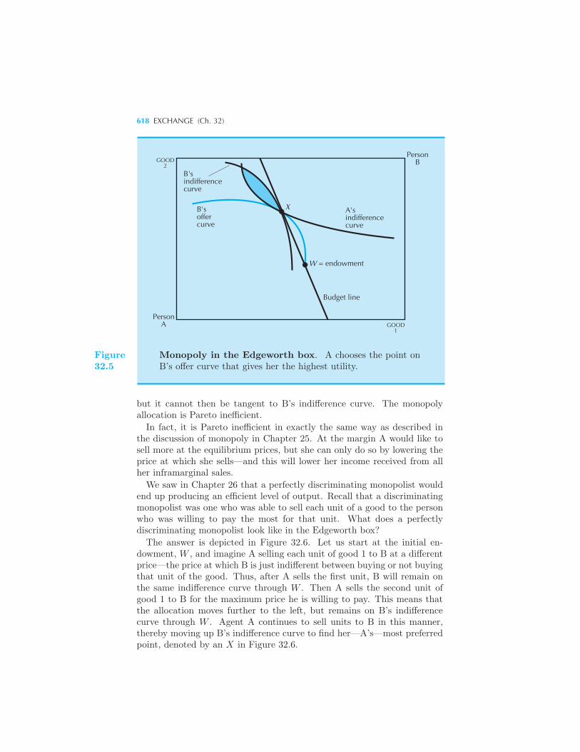
618 EXCHANGE (Ch. 32)
GOOD1
GOOD2
PersonA
PersonB
X
W = endowment
Budget line
A'sindifferencecurve
B'soffercurve
B'sindifferencecurve
Figure32.5
Monopoly in the Edgeworth box. A chooses the point onB’s offer curve that gives her the highest utility.
but it cannot then be tangent to B’s indifference curve. The monopolyallocation is Pareto inefficient.
In fact, it is Pareto inefficient in exactly the same way as described inthe discussion of monopoly in Chapter 25. At the margin A would like tosell more at the equilibrium prices, but she can only do so by lowering theprice at which she sells—and this will lower her income received from allher inframarginal sales.
We saw in Chapter 26 that a perfectly discriminating monopolist wouldend up producing an efficient level of output. Recall that a discriminatingmonopolist was one who was able to sell each unit of a good to the personwho was willing to pay the most for that unit. What does a perfectlydiscriminating monopolist look like in the Edgeworth box?
The answer is depicted in Figure 32.6. Let us start at the initial en-dowment, W , and imagine A selling each unit of good 1 to B at a differentprice—the price at which B is just indifferent between buying or not buyingthat unit of the good. Thus, after A sells the first unit, B will remain onthe same indifference curve through W . Then A sells the second unit ofgood 1 to B for the maximum price he is willing to pay. This means thatthe allocation moves further to the left, but remains on B’s indifferencecurve through W . Agent A continues to sell units to B in this manner,thereby moving up B’s indifference curve to find her—A’s—most preferredpoint, denoted by an X in Figure 32.6.
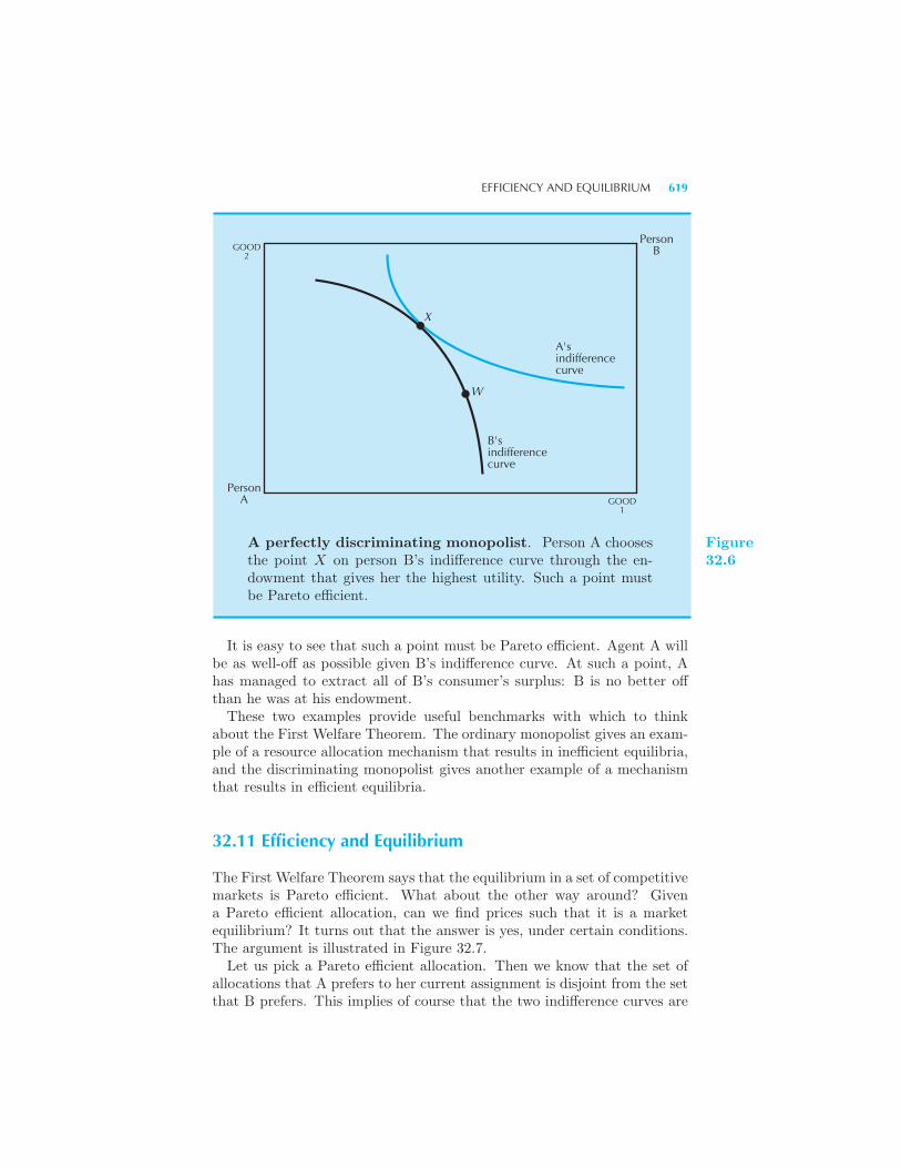
EFFICIENCY AND EQUILIBRIUM 619
GOOD2
X
W
PersonB
PersonA GOOD
1
A'sindifferencecurve
B'sindifferencecurve
A perfectly discriminating monopolist. Person A choosesthe point X on person B’s indifference curve through the en-dowment that gives her the highest utility. Such a point mustbe Pareto efficient.
Figure32.6
It is easy to see that such a point must be Pareto efficient. Agent A willbe as well-off as possible given B’s indifference curve. At such a point, Ahas managed to extract all of B’s consumer’s surplus: B is no better offthan he was at his endowment.These two examples provide useful benchmarks with which to think
about the First Welfare Theorem. The ordinary monopolist gives an exam-ple of a resource allocation mechanism that results in inefficient equilibria,and the discriminating monopolist gives another example of a mechanismthat results in efficient equilibria.
32.11 Efficiency and Equilibrium
The First Welfare Theorem says that the equilibrium in a set of competitivemarkets is Pareto efficient. What about the other way around? Givena Pareto efficient allocation, can we find prices such that it is a marketequilibrium? It turns out that the answer is yes, under certain conditions.The argument is illustrated in Figure 32.7.Let us pick a Pareto efficient allocation. Then we know that the set of
allocations that A prefers to her current assignment is disjoint from the setthat B prefers. This implies of course that the two indifference curves are
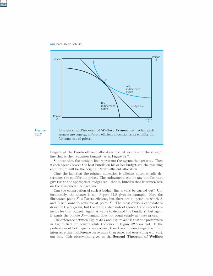
620 EXCHANGE (Ch. 32)
GOOD2
PersonB
GOOD1
X
A'sindifferencecurve
Budget lineB'sindifferencecurve
PersonA
Figure32.7
The Second Theorem of Welfare Economics. When pref-erences are convex, a Pareto efficient allocation is an equilibriumfor some set of prices.
tangent at the Pareto efficient allocation. So let us draw in the straightline that is their common tangent, as in Figure 32.7.
Suppose that the straight line represents the agents’ budget sets. Thenif each agent chooses the best bundle on his or her budget set, the resultingequilibrium will be the original Pareto efficient allocation.
Thus the fact that the original allocation is efficient automatically de-termines the equilibrium prices. The endowments can be any bundles thatgive rise to the appropriate budget set—that is, bundles that lie somewhereon the constructed budget line.
Can the construction of such a budget line always be carried out? Un-fortunately, the answer is no. Figure 32.8 gives an example. Here theillustrated point X is Pareto efficient, but there are no prices at which Aand B will want to consume at point X. The most obvious candidate isdrawn in the diagram, but the optimal demands of agents A and B don’t co-incide for that budget. Agent A wants to demand the bundle Y , but agentB wants the bundle X—demand does not equal supply at these prices.
The difference between Figure 32.7 and Figure 32.8 is that the preferencesin Figure 32.7 are convex while the ones in Figure 32.8 are not. If thepreferences of both agents are convex, then the common tangent will notintersect either indifference curve more than once, and everything will workout fine. This observation gives us the Second Theorem of Welfare
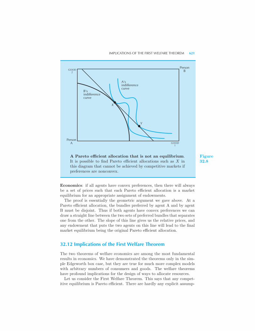
IMPLICATIONS OF THE FIRST WELFARE THEOREM 621
X
Y
PersonA GOOD
1
PersonB
A's indifferencecurve
B's indifferencecurve
GOOD2
A Pareto efficient allocation that is not an equilibrium.It is possible to find Pareto efficient allocations such as X inthis diagram that cannot be achieved by competitive markets ifpreferences are nonconvex.
Figure32.8
Economics: if all agents have convex preferences, then there will alwaysbe a set of prices such that each Pareto efficient allocation is a marketequilibrium for an appropriate assignment of endowments.The proof is essentially the geometric argument we gave above. At a
Pareto efficient allocation, the bundles preferred by agent A and by agentB must be disjoint. Thus if both agents have convex preferences we candraw a straight line between the two sets of preferred bundles that separatesone from the other. The slope of this line gives us the relative prices, andany endowment that puts the two agents on this line will lead to the finalmarket equilibrium being the original Pareto efficient allocation.
32.12 Implications of the First Welfare Theorem
The two theorems of welfare economics are among the most fundamentalresults in economics. We have demonstrated the theorems only in the sim-ple Edgeworth box case, but they are true for much more complex modelswith arbitrary numbers of consumers and goods. The welfare theoremshave profound implications for the design of ways to allocate resources.Let us consider the First Welfare Theorem. This says that any compet-
itive equilibrium is Pareto efficient. There are hardly any explicit assump-
622 EXCHANGE (Ch. 32)
tions in this theorem—it follows almost entirely from the definitions. Butthere are some implicit assumptions. One major assumption is that agentsonly care about their own consumption of goods, and not about what otheragents consume. If one agent does care about another agent’s consumption,we say that there is a consumption externality. We shall see that whenconsumption externalities are present, a competitive equilibrium need notbe Pareto efficient.To take a simple example, suppose that agent A cares about agent B’s
consumption of cigars. Then there is no particular reason why each agentchoosing his or her own consumption bundle at the market prices will resultin a Pareto efficient allocation. After each person has purchased the bestbundle he or she can afford, there may still be ways to make both of thembetter off—such as A paying B to smoke fewer cigars. We will discussexternalities in more detail in Chapter 35.Another important implicit assumption in the First Welfare Theorem
is that agents actually behave competitively. If there really were onlytwo agents, as in the Edgeworth box example, then it is unlikely thatthey would each take price as given. Instead, the agents would probablyrecognize their market power and would attempt to use their market powerto improve their own positions. The concept of competitive equilibriumonly makes sense when there are enough agents to ensure that each behavescompetitively.Finally, the First Welfare Theorem is only of interest if a competitive
equilibrium actually exists. As we have argued above, this will be the caseif the consumers are sufficiently small relative to the size of the market.Given these provisos, the First Welfare Theorem is a pretty strong result:
a private market, with each agent seeking to maximize his or her own utility,will result in an allocation that achieves Pareto efficiency.The importance of the First Welfare Theorem is that it gives a general
mechanism—the competitive market—that we can use to ensure Paretoefficient outcomes. If there are only two agents involved, this doesn’t mat-ter very much; it is easy for two people to get together and examine thepossibilities for mutual trades. But if there are thousands, or even mil-lions, of people involved there must be some kind of structure imposed onthe trading process. The First Welfare Theorem shows that the particularstructure of competitive markets has the desirable property of achieving aPareto efficient allocation.If we are dealing with a resource problem involving many people, it is
important to note that the use of competitive markets economizes on theinformation that any one agent needs to possess. The only things that aconsumer needs to know to make his consumption decisions are the pricesof the goods he is considering consuming. Consumers don’t need to knowanything about how the goods are produced, or who owns what goods, orwhere the goods come from in a competitive market. If each consumerknows only the prices of the goods, he can determine his demands, and if
IMPLICATIONS OF THE SECOND WELFARE THEOREM 623
the market functions well enough to determine the competitive prices, weare guaranteed an efficient outcome. The fact that competitive marketseconomize on information in this way is a strong argument in favor of theiruse as a way to allocate resources.
32.13 Implications of the Second Welfare Theorem
The Second Theorem of Welfare Economics asserts that under certain con-ditions, every Pareto efficient allocation can be achieved as a competitiveequilibrium.What is the meaning of this result? The Second Welfare Theorem implies
that the problems of distribution and efficiency can be separated. What-ever Pareto efficient allocation you want can be supported by the marketmechanism. The market mechanism is distributionally neutral; whateveryour criteria for a good or a just distribution of welfare, you can use com-petitive markets to achieve it.Prices play two roles in the market system: an allocative role and a
distributive role. The allocative role of prices is to indicate relative scarcity;the distributive role is to determine how much of different goods differentagents can purchase. The SecondWelfare Theorem says that these two rolescan be separated: we can redistribute endowments of goods to determinehow much wealth agents have, and then use prices to indicate relativescarcity.Policy discussions often become confused on this point. One often hears
arguments for intervening in pricing decisions on grounds of distributionalequity. However, such intervention is typically misguided. As we have seenabove, a convenient way to achieve efficient allocations is for each agentto face the true social costs of his or her actions and to make choices thatreflect those costs. Thus in a perfectly competitive market the marginaldecision of whether to consume more or less of some good will dependon the price—which measures how everyone else values this good on themargin. The considerations of efficiency are inherently marginal decisions—each person should face the correct marginal tradeoff in making his or herconsumption decisions.The decision about how much different agents should consume is a totally
different issue. In a competitive market this is determined by the value ofthe resources that a person has to sell. From the viewpoint of the puretheory, there is no reason why the state can’t transfer purchasing power—endowments—among consumers in any way that is seen fit.In fact the state doesn’t need to transfer the physical endowments them-
selves. All that is necessary is to transfer the purchasing power of theendowment. The state could tax one consumer on the basis of the value ofhis endowment and transfer this money to another. As long as the taxesare based on the value of the consumer’s endowment of goods there will
624 EXCHANGE (Ch. 32)
be no loss of efficiency. It is only when taxes depend on the choices that aconsumer makes that inefficiencies result, since in this case, the taxes willaffect the consumer’s marginal choices.It is true that a tax on endowments will generally change people’s behav-
ior. But, according to the First Welfare Theorem, trade from any initialendowments will result in a Pareto efficient allocation. Thus no matter howone redistributes endowments, the equilibrium allocation as determined bymarket forces will still be Pareto efficient.However, there are practical matters involved. It would be easy to have
a lump-sum tax on consumers. We could tax all consumers with blue eyes,and redistribute the proceeds to consumers with brown eyes. As long aseye color can’t be changed, there would be no loss in efficiency. Or we couldtax consumers with high IQs and redistribute the funds to consumers withlow IQs. Again, as long as IQ can be measured, there is no efficiency lossin this kind of tax.But there’s the problem. How do we measure people’s endowment of
goods? For most people, the bulk of their endowment consists of theirown labor power. People’s endowments of labor consist of the labor thatthey could consider selling, not the amount of labor that they actuallyend up selling. Taxing labor that people decide to sell to the market is adistortionary tax. If the sale of labor is taxed, the labor supply decisionof consumers will be distorted—they will likely supply less labor than theywould have supplied in the absence of a tax. Taxing the potential value oflabor—the endowment of labor—is not distortionary. The potential valueof labor is, by definition, something that is not changed by taxation. Taxingthe value of the endowment sounds easy until we realize that it involvesidentifying and taxing something that might be sold, rather than taxingsomething that is sold.We could imagine a mechanism for levying this kind of tax. Suppose
that we considered a society where each consumer was required to givethe money earned in 10 hours of his labor time to the state each week.This kind of tax would be independent of how much the person actuallyworked—it would only depend on the endowment of labor, not on howmuch was actually sold. Such a tax is basically transferring some part ofeach consumer’s endowment of labor time to the state. The state couldthen use these funds to provide various goods, or it could simply transferthese funds to other agents.According to the Second Welfare Theorem, this kind of lump-sum taxa-
tion would be nondistortionary. Essentially any Pareto efficient allocationcould be achieved by such lump-sum redistribution.However, no one is advocating such a radical restructuring of the tax
system. Most people’s labor supply decisions are relatively insensitive tovariations in the wage rate, so the efficiency loss from taxing labor may notbe too large anyway. But the message of the Second Welfare Theorem isimportant. Prices should be used to reflect scarcity. Lump-sum transfers of
SUMMARY 625
wealth should be used to adjust for distributional goals. To a large degree,these two policy decisions can be separated.People’s concern about the distribution of welfare can lead them to ad-
vocate various forms of manipulation of prices. It has been argued, forexample, that senior citizens should have access to less expensive telephoneservice, or that small users of electricity should pay lower rates than largeusers. These are basically attempts to redistribute income through theprice system by offering some people lower prices than others.When you think about it this is a terribly inefficient way to redistribute
income. If you want to redistribute income, why don’t you simply redis-tribute income? If you give a person an extra dollar to spend, then he canchoose to consume more of any of the goods that he wants to consume—notnecessarily just the good being subsidized.
Summary
1. General equilibrium refers to the study of how the economy can adjustto have demand equal supply in all markets at the same time.
2. The Edgeworth box is a graphical tool to examine such a general equi-librium with 2 consumers and 2 goods.
3. A Pareto efficient allocation is one in which there is no feasible reallo-cation of the goods that would make all consumers at least as well-off andat least one consumer strictly better off.
4. Walras’ law states that the value of aggregate excess demand is zero forall prices.
5. A general equilibrium allocation is one in which each agent chooses amost preferred bundle of goods from the set of goods that he or she canafford.
6. Only relative prices are determined in a general equilibrium system.
7. If the demand for each good varies continuously as prices vary, thenthere will always be some set of prices where demand equals supply inevery market; that is, a competitive equilibrium.
8. The First Theorem of Welfare Economics states that a competitive equi-librium is Pareto efficient.
9. The Second Theorem of Welfare Economics states that as long as pref-erences are convex, then every Pareto efficient allocation can be supportedas a competitive equilibrium.
626 EXCHANGE (Ch. 32)
REVIEW QUESTIONS
1. Is it possible to have a Pareto efficient allocation where someone is worseoff than he is at an allocation that is not Pareto efficient?
2. Is it possible to have a Pareto efficient allocation where everyone is worseoff than they are at an allocation that is not Pareto efficient?
3. True or false? If we know the contract curve, then we know the outcomeof any trading.
4. Can some individual be made better off if we are at a Pareto efficientallocation?
5. If the value of excess demand in 8 out of 10 markets is equal to zero,what must be true about the remaining two markets?
APPENDIX
Let us examine the calculus conditions describing Pareto efficient allocations. Bydefinition, a Pareto efficient allocation makes each agent as well-off as possible,given the utility of the other agent. So let us pick u as the utility level for agentB, say, and see how we can make agent A as well-off as possible.
The maximization problem is
maxx1A,x2
A,x1
B,x2
B
uA(x1A, x
2A)
such that uB(x1B , x
2B) = u
x1A + x1
B = ω1
x2A + x2
B = ω2.
Here ω1 = ω1A+ω1
B is the total amount of good 1 available and ω2 = ω2A+ω2
B isthe total amount of good 2 available. This maximization problem asks us to findthe allocation (x1
A, x2A, x
1B , x
2B) that makes person A’s utility as large as possible,
given a fixed level for person B’s utility, and given that the total amount of eachgood used is equal to the amount available.
We can write the Lagrangian for this problem as
L = uA(x1A, x
2A)− λ(uB(x
1B , x
2B)− u)
− μ1(x1A + x1
B − ω1)− μ2(x2A + x2
B − ω2).
Here λ is the Lagrange multiplier on the utility constraint, and the μ’s arethe Lagrange multipliers on the resource constraints. When we differentiate with
APPENDIX 627
respect to each of the goods, we have four first-order conditions that must holdat the optimal solution:
∂L
∂x1A
=∂uA
∂x1A
− μ1 = 0
∂L
∂x2A
=∂uA
∂x2A
− μ2 = 0
∂L
∂x1B
= −λ∂uB
∂x1B
− μ1 = 0
∂L
∂x2B
= −λ∂uB
∂x2B
− μ2 = 0.
If we divide the first equation by the second, and the third equation by thefourth, we have
MRSA =∂uA/∂x
1A
∂uA/∂x2A
=μ1
μ2(32.5)
MRSB =∂uB/∂x
1B
∂uB/∂x2B
=μ1
μ2. (32.6)
The interpretation of these conditions is given in the text: at a Pareto efficientallocation, the marginal rates of substitution between the two goods must be thesame. Otherwise, there would be some trade that would make each consumerbetter off.
Let us recall the conditions that must hold for optimal choice by consumers. Ifconsumer A is maximizing utility subject to her budget constraint and consumerB is maximizing utility subject to his budget constraint, and both consumers facethe same prices for goods 1 and 2, we must have
∂uA/∂x1A
∂uA/∂x2A
=p1p2
(32.7)
∂uB/∂x1B
∂uB/∂x2B
=p1p2
. (32.8)
Note the similarity with the efficiency conditions. The Lagrange multipliers in theefficiency conditions, μ1 and μ2, are just like the prices p1 and p2 in the consumerchoice conditions. In fact the Lagrange multipliers in this kind of problem aresometimes known as shadow prices or efficiency prices.
Every Pareto efficient allocation has to satisfy conditions like those in equations(32.5) and (32.6). Every competitive equilibrium has to satisfy conditions likethose in equations (32.7) and (32.8). The conditions describing Pareto efficiencyand the conditions describing individual maximization in a market environmentare virtually the same.
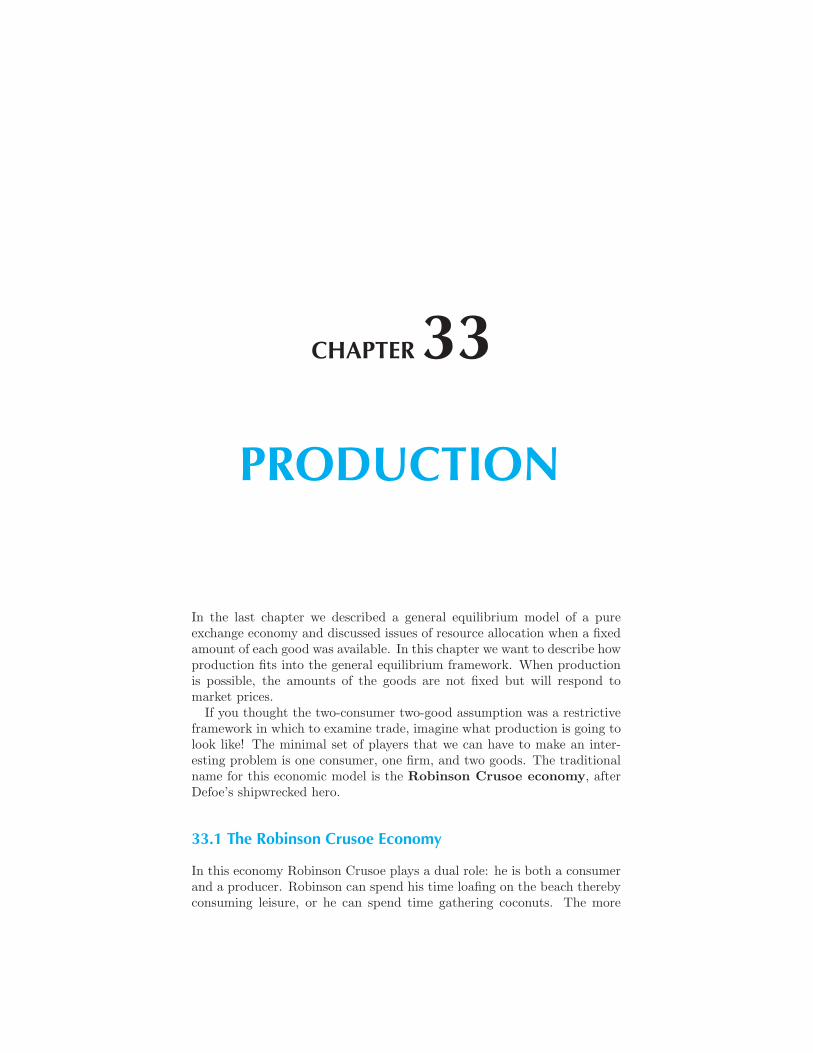
CHAPTER 33
PRODUCTION
In the last chapter we described a general equilibrium model of a pureexchange economy and discussed issues of resource allocation when a fixedamount of each good was available. In this chapter we want to describe howproduction fits into the general equilibrium framework. When productionis possible, the amounts of the goods are not fixed but will respond tomarket prices.If you thought the two-consumer two-good assumption was a restrictive
framework in which to examine trade, imagine what production is going tolook like! The minimal set of players that we can have to make an inter-esting problem is one consumer, one firm, and two goods. The traditionalname for this economic model is the Robinson Crusoe economy, afterDefoe’s shipwrecked hero.
33.1 The Robinson Crusoe Economy
In this economy Robinson Crusoe plays a dual role: he is both a consumerand a producer. Robinson can spend his time loafing on the beach therebyconsuming leisure, or he can spend time gathering coconuts. The more
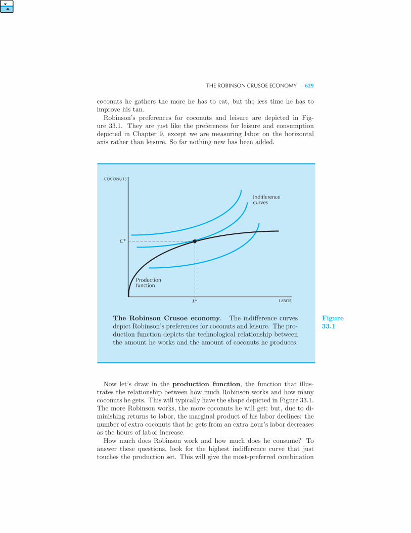
THE ROBINSON CRUSOE ECONOMY 629
coconuts he gathers the more he has to eat, but the less time he has toimprove his tan.Robinson’s preferences for coconuts and leisure are depicted in Fig-
ure 33.1. They are just like the preferences for leisure and consumptiondepicted in Chapter 9, except we are measuring labor on the horizontalaxis rather than leisure. So far nothing new has been added.
COCONUTS
C*
Productionfunction
L* LABOR
Indifferencecurves
The Robinson Crusoe economy. The indifference curvesdepict Robinson’s preferences for coconuts and leisure. The pro-duction function depicts the technological relationship betweenthe amount he works and the amount of coconuts he produces.
Figure33.1
Now let’s draw in the production function, the function that illus-trates the relationship between how much Robinson works and how manycoconuts he gets. This will typically have the shape depicted in Figure 33.1.The more Robinson works, the more coconuts he will get; but, due to di-minishing returns to labor, the marginal product of his labor declines: thenumber of extra coconuts that he gets from an extra hour’s labor decreasesas the hours of labor increase.How much does Robinson work and how much does he consume? To
answer these questions, look for the highest indifference curve that justtouches the production set. This will give the most-preferred combination
630 PRODUCTION (Ch. 33)
of labor and consumption that Robinson can get, given the technology forgathering coconuts that he is using.At this point, the slope of the indifference curve must equal the slope of
the production function by the standard argument: if they crossed, therewould be some other feasible point that was preferred. This means that themarginal product of an extra hour of labor must equal the marginal rateof substitution between leisure and coconuts. If the marginal product weregreater than the marginal rate of substitution, it would pay for Robinsonto give up a little leisure in order to get the extra coconuts. If the marginalproduct were less than the marginal rate of substitution, it would pay forRobinson to work a little less.
33.2 Crusoe, Inc.
So far this story is only a slight extension of models we have already seen.But now let’s add a new feature. Suppose that Robinson is tired of si-multaneously being a producer and consumer and that he decides to al-ternate roles. One day he will behave entirely as a producer, and thenext day he will behave entirely as a consumer. In order to coordinatethese activities, he decides to set up a labor market and a coconut mar-ket.He also sets up a firm, Crusoe, Inc., and becomes its sole shareholder.
The firm is going to look at the prices for labor and coconuts and decidehow much labor to hire and how many coconuts to produce, guided bythe principle of profit maximization. Robinson, in his role as a worker,is going to collect income from working at the firm; in his role as share-holder in the firm he will collect profits; and, in his role as consumer hewill decide how much to purchase of the firm’s output. (No doubt thissounds peculiar, but there really isn’t that much else to do on a desertisland.)In order to keep track of his transactions, Robinson invents a currency
he calls “dollars,” and he chooses, somewhat arbitrarily, to set the price ofcoconuts at one dollar apiece. Thus coconuts are the numeraire good forthis economy; as we’ve seen in Chapter 2, a numeraire good is one whoseprice has been set to one. Since the price of coconuts is normalized at one,we have only to determine the wage rate. What should his wage rate be inorder to make this market work?We’re going to think about this problem first from the viewpoint of
Crusoe, Inc., and then from the viewpoint of Robinson, the consumer. Thediscussion is a little schizophrenic at times, but that’s what you have toput up with if you want to have an economy with only one person. We’regoing to look at the economy after it has been running along for some time,and everything is in equilibrium. In equilibrium, the demand for coconutswill equal the supply of coconuts and the demand for labor will equal the
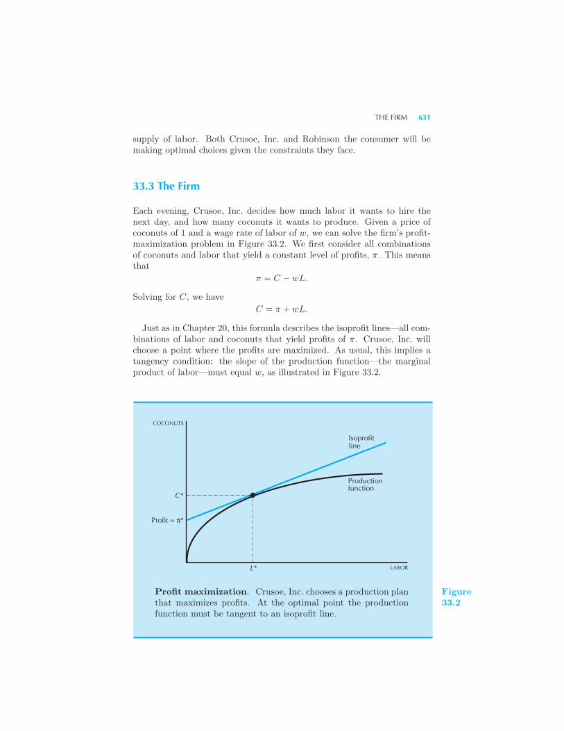
THE FIRM 631
supply of labor. Both Crusoe, Inc. and Robinson the consumer will bemaking optimal choices given the constraints they face.
33.3 The Firm
Each evening, Crusoe, Inc. decides how much labor it wants to hire thenext day, and how many coconuts it wants to produce. Given a price ofcoconuts of 1 and a wage rate of labor of w, we can solve the firm’s profit-maximization problem in Figure 33.2. We first consider all combinationsof coconuts and labor that yield a constant level of profits, π. This meansthat
π = C − wL.
Solving for C, we have
C = π + wL.
Just as in Chapter 20, this formula describes the isoprofit lines—all com-binations of labor and coconuts that yield profits of π. Crusoe, Inc. willchoose a point where the profits are maximized. As usual, this implies atangency condition: the slope of the production function—the marginalproduct of labor—must equal w, as illustrated in Figure 33.2.
C*
Profit = π*
LABOR
COCONUTS
Isoprofitline
Productionfunction
L*
Profit maximization. Crusoe, Inc. chooses a production planthat maximizes profits. At the optimal point the productionfunction must be tangent to an isoprofit line.
Figure33.2
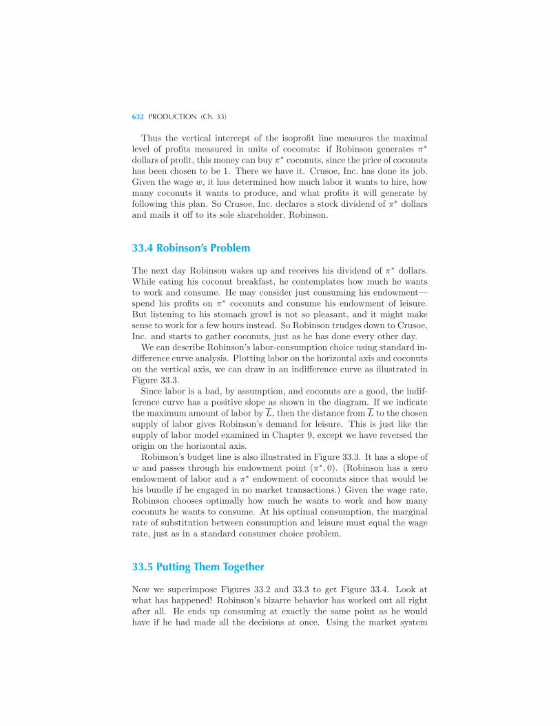
632 PRODUCTION (Ch. 33)
Thus the vertical intercept of the isoprofit line measures the maximallevel of profits measured in units of coconuts: if Robinson generates π∗
dollars of profit, this money can buy π∗ coconuts, since the price of coconutshas been chosen to be 1. There we have it. Crusoe, Inc. has done its job.Given the wage w, it has determined how much labor it wants to hire, howmany coconuts it wants to produce, and what profits it will generate byfollowing this plan. So Crusoe, Inc. declares a stock dividend of π∗ dollarsand mails it off to its sole shareholder, Robinson.
33.4 Robinson’s Problem
The next day Robinson wakes up and receives his dividend of π∗ dollars.While eating his coconut breakfast, he contemplates how much he wantsto work and consume. He may consider just consuming his endowment—spend his profits on π∗ coconuts and consume his endowment of leisure.But listening to his stomach growl is not so pleasant, and it might makesense to work for a few hours instead. So Robinson trudges down to Crusoe,Inc. and starts to gather coconuts, just as he has done every other day.We can describe Robinson’s labor-consumption choice using standard in-
difference curve analysis. Plotting labor on the horizontal axis and coconutson the vertical axis, we can draw in an indifference curve as illustrated inFigure 33.3.Since labor is a bad, by assumption, and coconuts are a good, the indif-
ference curve has a positive slope as shown in the diagram. If we indicatethe maximum amount of labor by L, then the distance from L to the chosensupply of labor gives Robinson’s demand for leisure. This is just like thesupply of labor model examined in Chapter 9, except we have reversed theorigin on the horizontal axis.Robinson’s budget line is also illustrated in Figure 33.3. It has a slope of
w and passes through his endowment point (π∗, 0). (Robinson has a zeroendowment of labor and a π∗ endowment of coconuts since that would behis bundle if he engaged in no market transactions.) Given the wage rate,Robinson chooses optimally how much he wants to work and how manycoconuts he wants to consume. At his optimal consumption, the marginalrate of substitution between consumption and leisure must equal the wagerate, just as in a standard consumer choice problem.
33.5 Putting Them Together
Now we superimpose Figures 33.2 and 33.3 to get Figure 33.4. Look atwhat has happened! Robinson’s bizarre behavior has worked out all rightafter all. He ends up consuming at exactly the same point as he wouldhave if he had made all the decisions at once. Using the market system
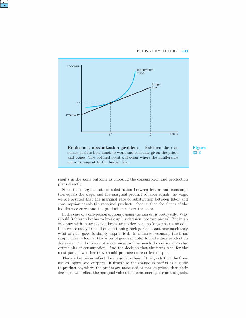
PUTTING THEM TOGETHER 633
LABORLL*
Profit = π*
C*
Budgetline
Indifferencecurve
COCONUTS
Robinson’s maximization problem. Robinson the con-sumer decides how much to work and consume given the pricesand wages. The optimal point will occur where the indifferencecurve is tangent to the budget line.
Figure33.3
results in the same outcome as choosing the consumption and productionplans directly.
Since the marginal rate of substitution between leisure and consump-tion equals the wage, and the marginal product of labor equals the wage,we are assured that the marginal rate of substitution between labor andconsumption equals the marginal product—that is, that the slopes of theindifference curve and the production set are the same.
In the case of a one-person economy, using the market is pretty silly. Whyshould Robinson bother to break up his decision into two pieces? But in aneconomy with many people, breaking up decisions no longer seems so odd.If there are many firms, then questioning each person about how much theywant of each good is simply impractical. In a market economy the firmssimply have to look at the prices of goods in order to make their productiondecisions. For the prices of goods measure how much the consumers valueextra units of consumption. And the decision that the firms face, for themost part, is whether they should produce more or less output.
The market prices reflect the marginal values of the goods that the firmsuse as inputs and outputs. If firms use the change in profits as a guideto production, where the profits are measured at market prices, then theirdecisions will reflect the marginal values that consumers place on the goods.
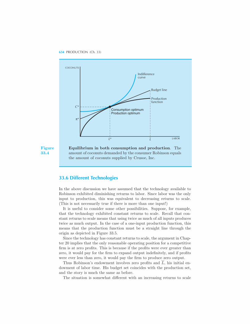
634 PRODUCTION (Ch. 33)
C*
COCONUTS
Indifferencecurve
Budget line
Productionfunction
Consumption optimumProduction optimum
L* L LABOR
π*
Figure33.4
Equilibrium in both consumption and production. Theamount of coconuts demanded by the consumer Robinson equalsthe amount of coconuts supplied by Crusoe, Inc.
33.6 Different Technologies
In the above discussion we have assumed that the technology available toRobinson exhibited diminishing returns to labor. Since labor was the onlyinput to production, this was equivalent to decreasing returns to scale.(This is not necessarily true if there is more than one input!)It is useful to consider some other possibilities. Suppose, for example,
that the technology exhibited constant returns to scale. Recall that con-stant returns to scale means that using twice as much of all inputs producestwice as much output. In the case of a one-input production function, thismeans that the production function must be a straight line through theorigin as depicted in Figure 33.5.Since the technology has constant returns to scale, the argument in Chap-
ter 20 implies that the only reasonable operating position for a competitivefirm is at zero profits. This is because if the profits were ever greater thanzero, it would pay for the firm to expand output indefinitely, and if profitswere ever less than zero, it would pay the firm to produce zero output.Thus Robinson’s endowment involves zero profits and L, his initial en-
dowment of labor time. His budget set coincides with the production set,and the story is much the same as before.The situation is somewhat different with an increasing returns to scale
DIFFERENT TECHNOLOGIES 635
COCONUTS
C*
L* L
Indifferencecurve
Budget line =productionfunction
LABOR
Constant returns to scale. If the technology exhibits con-stant returns to scale, Crusoe, Inc., makes zero profits.
Figure33.5
technology, as depicted in Figure 33.6. There is no difficulty in this simpleexample in exhibiting the optimal choice of consumption and leisure forRobinson. The indifference curve will be tangent to the production setas usual. The problem arises in trying to support this point as a profit-maximizing point. For if the firm were faced with the prices given byRobinson’s marginal rate of substitution, it would want to produce moreoutput than Robinson would demand.
If the firm exhibits increasing returns to scale at the optimal choice,then the average costs of production will exceed the marginal costs ofproduction—and that means that the firm will be making negative profits.The goal of profit maximization would lead the firm to want to increaseits output—but this would be incompatible with the demands for outputand the supplies of inputs from the consumers. In the case depicted, thereis no price at which the utility-maximizing demand by the consumer willequal the profit-maximizing supply from the firm.
Increasing returns to scale is an example of a nonconvexity. In thiscase the production set—the set of coconuts and labor that are feasiblefor the economy—is not a convex set. Thus the common tangent to theindifference curve and the production function at the point (L∗, C∗) inFigure 33.6 will not separate the preferred points from the feasible pointsas it does in Figure 33.4.
Nonconvexities such as this pose grave difficulties for the functioning ofcompetitive markets. In a competitive market consumers and firms look
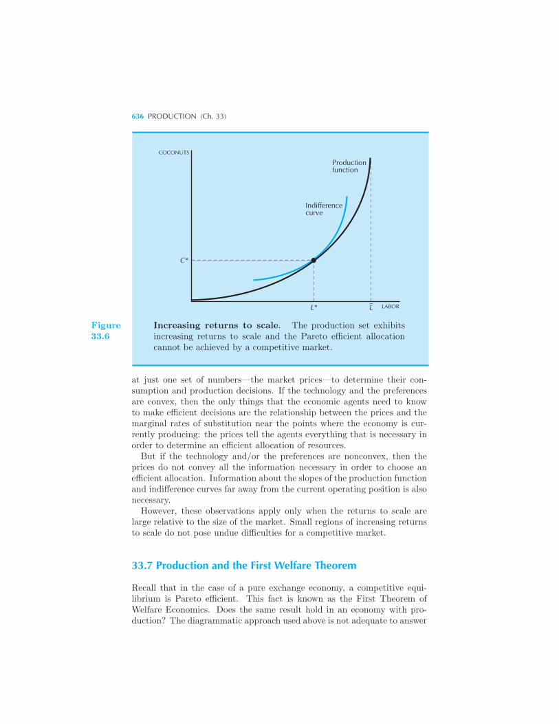
636 PRODUCTION (Ch. 33)
COCONUTS
C*
L* L LABOR
Productionfunction
Indifferencecurve
Figure33.6
Increasing returns to scale. The production set exhibitsincreasing returns to scale and the Pareto efficient allocationcannot be achieved by a competitive market.
at just one set of numbers—the market prices—to determine their con-sumption and production decisions. If the technology and the preferencesare convex, then the only things that the economic agents need to knowto make efficient decisions are the relationship between the prices and themarginal rates of substitution near the points where the economy is cur-rently producing: the prices tell the agents everything that is necessary inorder to determine an efficient allocation of resources.But if the technology and/or the preferences are nonconvex, then the
prices do not convey all the information necessary in order to choose anefficient allocation. Information about the slopes of the production functionand indifference curves far away from the current operating position is alsonecessary.However, these observations apply only when the returns to scale are
large relative to the size of the market. Small regions of increasing returnsto scale do not pose undue difficulties for a competitive market.
33.7 Production and the First Welfare Theorem
Recall that in the case of a pure exchange economy, a competitive equi-librium is Pareto efficient. This fact is known as the First Theorem ofWelfare Economics. Does the same result hold in an economy with pro-duction? The diagrammatic approach used above is not adequate to answer
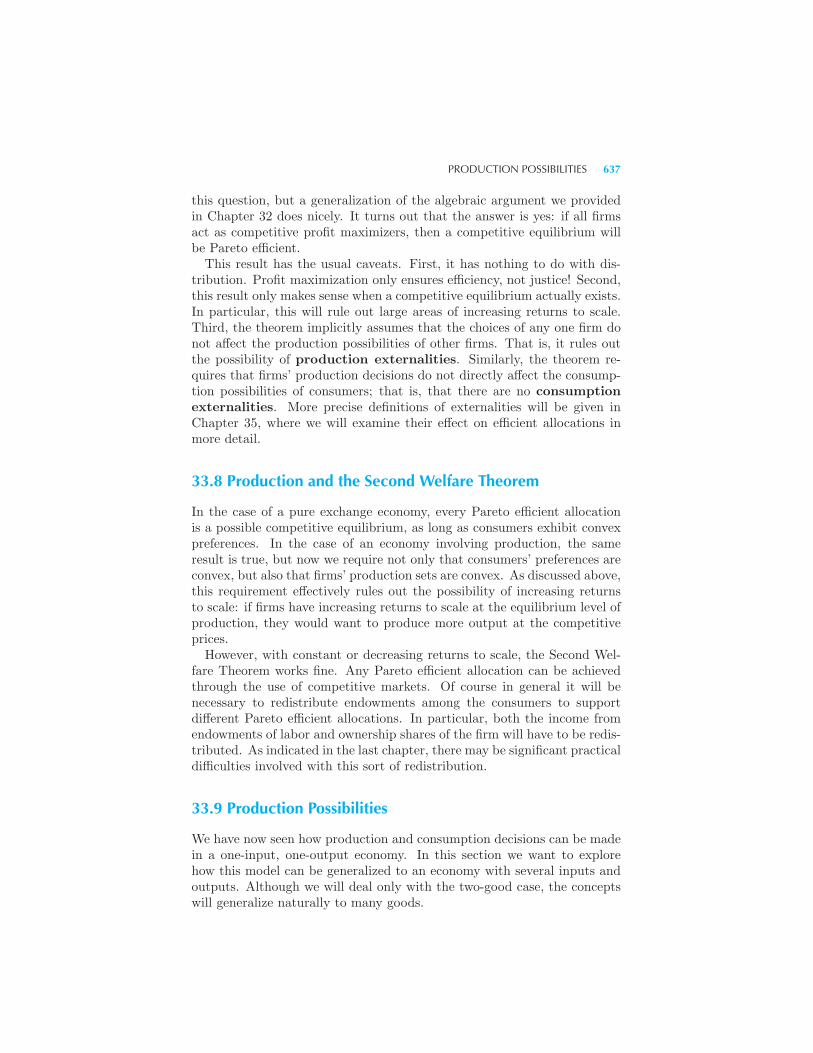
PRODUCTION POSSIBILITIES 637
this question, but a generalization of the algebraic argument we providedin Chapter 32 does nicely. It turns out that the answer is yes: if all firmsact as competitive profit maximizers, then a competitive equilibrium willbe Pareto efficient.This result has the usual caveats. First, it has nothing to do with dis-
tribution. Profit maximization only ensures efficiency, not justice! Second,this result only makes sense when a competitive equilibrium actually exists.In particular, this will rule out large areas of increasing returns to scale.Third, the theorem implicitly assumes that the choices of any one firm donot affect the production possibilities of other firms. That is, it rules outthe possibility of production externalities. Similarly, the theorem re-quires that firms’ production decisions do not directly affect the consump-tion possibilities of consumers; that is, that there are no consumptionexternalities. More precise definitions of externalities will be given inChapter 35, where we will examine their effect on efficient allocations inmore detail.
33.8 Production and the Second Welfare Theorem
In the case of a pure exchange economy, every Pareto efficient allocationis a possible competitive equilibrium, as long as consumers exhibit convexpreferences. In the case of an economy involving production, the sameresult is true, but now we require not only that consumers’ preferences areconvex, but also that firms’ production sets are convex. As discussed above,this requirement effectively rules out the possibility of increasing returnsto scale: if firms have increasing returns to scale at the equilibrium level ofproduction, they would want to produce more output at the competitiveprices.However, with constant or decreasing returns to scale, the Second Wel-
fare Theorem works fine. Any Pareto efficient allocation can be achievedthrough the use of competitive markets. Of course in general it will benecessary to redistribute endowments among the consumers to supportdifferent Pareto efficient allocations. In particular, both the income fromendowments of labor and ownership shares of the firm will have to be redis-tributed. As indicated in the last chapter, there may be significant practicaldifficulties involved with this sort of redistribution.
33.9 Production Possibilities
We have now seen how production and consumption decisions can be madein a one-input, one-output economy. In this section we want to explorehow this model can be generalized to an economy with several inputs andoutputs. Although we will deal only with the two-good case, the conceptswill generalize naturally to many goods.
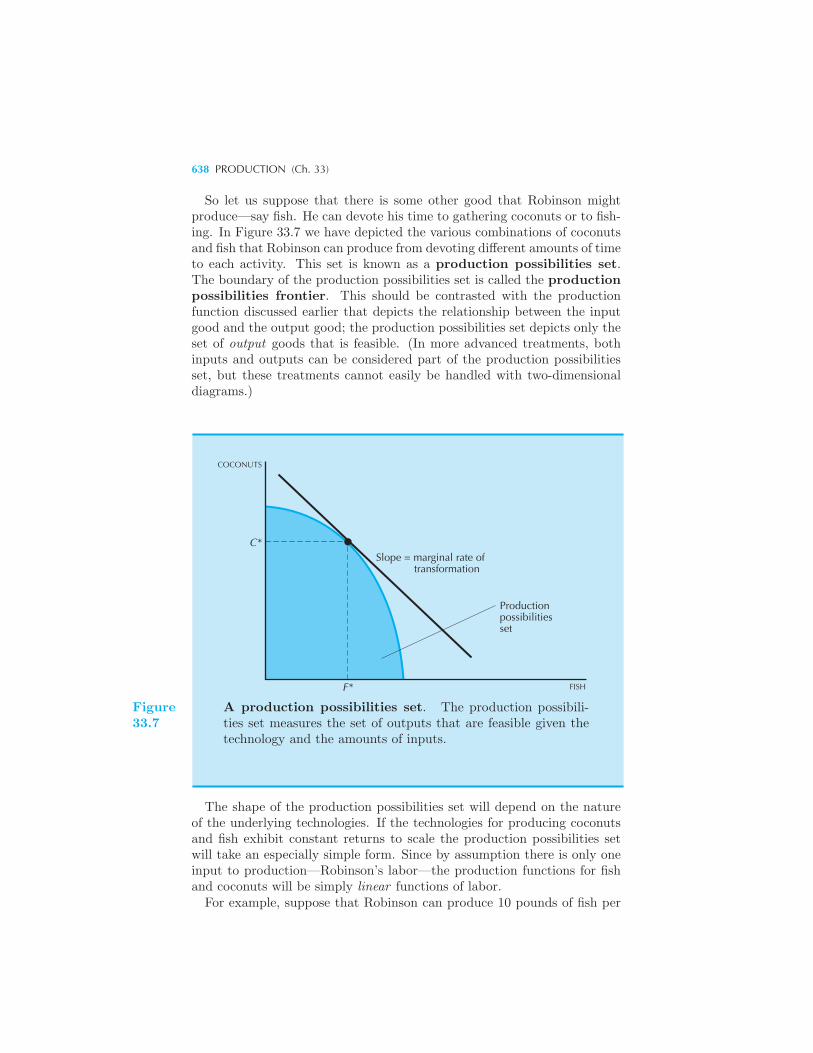
638 PRODUCTION (Ch. 33)
So let us suppose that there is some other good that Robinson mightproduce—say fish. He can devote his time to gathering coconuts or to fish-ing. In Figure 33.7 we have depicted the various combinations of coconutsand fish that Robinson can produce from devoting different amounts of timeto each activity. This set is known as a production possibilities set.The boundary of the production possibilities set is called the productionpossibilities frontier. This should be contrasted with the productionfunction discussed earlier that depicts the relationship between the inputgood and the output good; the production possibilities set depicts only theset of output goods that is feasible. (In more advanced treatments, bothinputs and outputs can be considered part of the production possibilitiesset, but these treatments cannot easily be handled with two-dimensionaldiagrams.)
COCONUTS
Slope = marginal rate of transformation
Productionpossibilitiesset
FISHF*
C*
Figure33.7
A production possibilities set. The production possibili-ties set measures the set of outputs that are feasible given thetechnology and the amounts of inputs.
The shape of the production possibilities set will depend on the natureof the underlying technologies. If the technologies for producing coconutsand fish exhibit constant returns to scale the production possibilities setwill take an especially simple form. Since by assumption there is only oneinput to production—Robinson’s labor—the production functions for fishand coconuts will be simply linear functions of labor.
For example, suppose that Robinson can produce 10 pounds of fish per
COMPARATIVE ADVANTAGE 639
hour or 20 pounds of coconuts per hour. Then if he devotes Lf hoursto fish production and Lc hours to coconut production, he will produce10Lf pounds of fish and 20Lc pounds of coconuts. Suppose that Robinsondecides to work 10 hours a day. Then the production possibilities set willconsist of all combinations of coconuts, C, and fish, F , such that
F = 10Lf
C = 20Lc
Lc + Lf = 10.
The first two equations measure the production relationships, and thethird measures the resource constraint. To determine the production pos-sibilities frontier solve the first two equations for Lf and Lc to get
Lf =F
10
Lc =C
20.
Now add these two equations together, and use the fact that Lf +Lc = 10to find
F
10+
C
20= 10.
This equation gives us all the combinations of fish and coconuts that Robin-son can produce if he works 10 hours a day. It is depicted in Figure 33.8A.The slope of this production possibilities set measures the marginal
rate of transformation—how much of one good Robinson can get if hedecides to sacrifice some of the other good. If Robinson gives up enoughlabor to produce 1 less pound of fish, he will be able to get 2 more poundsof coconuts. Think about it: if Robinson works one hour less on fishproduction, he will get 10 pounds less fish. But then if he devotes thattime to coconuts, he will get 20 pounds more coconuts. The tradeoff is ata ratio of 2 to 1.
33.10 Comparative Advantage
The construction of the production possibilities set given above was quitesimple since there was only one way to produce fish and one way to producecoconuts. What if there is more than one way to produce each good? Sup-pose that we add another worker to our island economy, who has differentskills in producing fish and coconuts.To be specific, let us call the new worker Friday, and suppose that he
can produce 20 pounds of fish per hour, or 10 pounds of coconuts per hour.
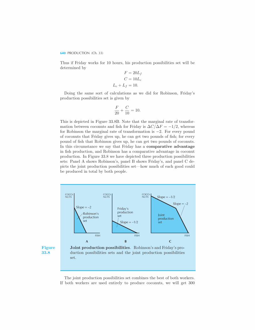
640 PRODUCTION (Ch. 33)
Thus if Friday works for 10 hours, his production possibilities set will bedetermined by
F = 20Lf
C = 10Lc
Lc + Lf = 10.
Doing the same sort of calculations as we did for Robinson, Friday’sproduction possibilities set is given by
F
20+
C
10= 10.
This is depicted in Figure 33.8B. Note that the marginal rate of transfor-mation between coconuts and fish for Friday is ΔC/ΔF = −1/2, whereasfor Robinson the marginal rate of transformation is −2. For every poundof coconuts that Friday gives up, he can get two pounds of fish; for everypound of fish that Robinson gives up, he can get two pounds of coconuts.In this circumstance we say that Friday has a comparative advantagein fish production, and Robinson has a comparative advantage in coconutproduction. In Figure 33.8 we have depicted three production possibilitiessets: Panel A shows Robinson’s, panel B shows Friday’s, and panel C de-picts the joint production possibilities set—how much of each good couldbe produced in total by both people.
FISH FISH FISH
COCO-NUTS
COCO-NUTS
COCO-NUTS
Slope = –2
Robinson'sproductionset
Friday'sproductionset Joint
productionset
Slope = –2
Slope = –1/2
Slope = –1/2
A B C
Figure33.8
Joint production possibilities. Robinson’s and Friday’s pro-duction possibilities sets and the joint production possibilitiesset.
The joint production possibilities set combines the best of both workers.If both workers are used entirely to produce coconuts, we will get 300
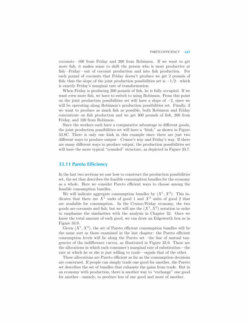
PARETO EFFICIENCY 641
coconuts—100 from Friday and 200 from Robinson. If we want to getmore fish, it makes sense to shift the person who is most productive atfish—Friday—out of coconut production and into fish production. Foreach pound of coconuts that Friday doesn’t produce we get 2 pounds offish; thus the slope of the joint production possibilities set is −1/2—whichis exactly Friday’s marginal rate of transformation.When Friday is producing 200 pounds of fish, he is fully occupied. If we
want even more fish, we have to switch to using Robinson. From this pointon the joint production possibilities set will have a slope of −2, since wewill be operating along Robinson’s production possibilities set. Finally, ifwe want to produce as much fish as possible, both Robinson and Fridayconcentrate on fish production and we get 300 pounds of fish, 200 fromFriday, and 100 from Robinson.Since the workers each have a comparative advantage in different goods,
the joint production possibilities set will have a “kink,” as shown in Figure33.8C. There is only one kink in this example since there are just twodifferent ways to produce output—Crusoe’s way and Friday’s way. If thereare many different ways to produce output, the production possibilities setwill have the more typical “rounded” structure, as depicted in Figure 33.7.
33.11 Pareto Efficiency
In the last two sections we saw how to construct the production possibilitiesset, the set that describes the feasible consumption bundles for the economyas a whole. Here we consider Pareto efficient ways to choose among thefeasible consumption bundles.We will indicate aggregate consumption bundles by (X1, X2). This in-
dicates that there are X1 units of good 1 and X2 units of good 2 thatare available for consumption. In the Crusoe/Friday economy, the twogoods are coconuts and fish, but we will use the (X1, X2) notation in orderto emphasize the similarities with the analysis in Chapter 32. Once weknow the total amount of each good, we can draw an Edgeworth box as inFigure 33.9.Given (X1, X2), the set of Pareto efficient consumption bundles will be
the same sort as those examined in the last chapter: the Pareto efficientconsumption levels will lie along the Pareto set—the line of mutual tan-gencies of the indifference curves, as illustrated in Figure 33.9. These arethe allocations in which each consumer’s marginal rate of substitution—therate at which he or she is just willing to trade—equals that of the other.These allocations are Pareto efficient as far as the consumption decisions
are concerned. If people can simply trade one good for another, the Paretoset describes the set of bundles that exhausts the gains from trade. But inan economy with production, there is another way to “exchange” one goodfor another—namely, to produce less of one good and more of another.
642 PRODUCTION (Ch. 33)
Slope = MRT
Paretoset
GOOD2
Slope = MRSProductionpossibilitiesset
GOOD1
Equilibriumproduction2x
Equilibriumconsumption
x1
Figure33.9
Production and the Edgeworth box. At each point on theproduction possibilities frontier, we can draw an Edgeworth boxto illustrate the possible consumption allocations.
The Pareto set describes the set of Pareto efficient bundles given theamounts of goods 1 and 2 available, but in an economy with productionthose amounts can themselves be chosen out of the production possibilitiesset. Which choices from the production possibilities set will be Paretoefficient choices?Let us think about the logic underlying the marginal rate of substitution
condition. We argued that in a Pareto efficient allocation, the MRS ofconsumer A had to be equal to the MRS of consumer B: the rate at whichconsumer A would just be willing to trade one good for the other shouldbe equal to the rate at which consumer B would just be willing to tradeone good for the other. If this were not true, then there would be sometrade that would make both consumers better off.Recall that the marginal rate of transformation (MRT) measures the
rate at which one good can be “transformed” into the other. Of course,one good really isn’t being literally transformed into the other. Rather thefactors of production are being moved around so as to produce less of onegood and more of the other.Suppose that the economy were operating at a position where the mar-
ginal rate of substitution of one of the consumers was not equal to themarginal rate of transformation between the two goods. Then such a po-sition cannot be Pareto efficient. Why? Because at this point, the rate at
CASTAWAYS, INC. 643
which the consumer is willing to trade good 1 for good 2 is different fromthe rate at which good 1 can be transformed into good 2—there is a wayto make the consumer better off by rearranging the pattern of production.Suppose, for example, that the consumer’s MRS is 1; the consumer is
just willing to substitute good 1 for good 2 on a one-to-one basis. Supposethat the MRT is 2, which means that giving up one unit of good 1 willallow society to produce two units of good 2. Then clearly it makes senseto reduce the production of good 1 by one unit; this will generate two extraunits of good 2. Since the consumer was just indifferent between giving upone unit of good 1 and getting one unit of the other good in exchange, heor she will now certainly be better off by getting two extra units of good 2.The same argument can be made whenever one of the consumers has a
MRS that is different from the MRT—there will always be a rearrangementof consumption and production that will make that consumer better off. Wehave already seen that for Pareto efficiency each consumer’s MRS shouldbe the same, and the argument given above implies that each consumer’sMRS should in fact be equal to the MRT.Figure 33.9 illustrates a Pareto efficient allocation. The MRSs of each
consumer are the same, since their indifference curves are tangent in theEdgeworth box. And each consumer’s MRS is equal to the MRT—the slopeof the production possibilities set.
33.12 Castaways, Inc.
In the last section we derived the necessary conditions for Pareto effi-ciency: the MRS of each consumer must equal the MRT. Any way ofdistributing resources that results in Pareto efficiency must satisfy thiscondition. Earlier in this chapter, we claimed that a competitive economywith profit-maximizing firms and utility-maximizing consumers would re-sult in a Pareto efficient allocation. In this section we explore the detailsof how this works.Our economy now contains two individuals, Robinson and Friday. There
are four goods: two factors of production (Robinson’s labor and Friday’slabor) and two output goods (coconuts and fish). Let us suppose thatRobinson and Friday are both shareholders of the firm, which we will nowrefer to as Castaways, Inc. Of course, they are also the sole employeesand customers, but as usual we shall examine each role in turn, and notallow the participants to see the wider picture. After all, the object of theanalysis is to understand how a decentralized resource allocation systemworks—one in which each person only has to determine his or her owndecisions, without regard for the functioning of the economy as a whole.Start first with Castaways, Inc., and consider the profit-maximization
problem. Castaways, Inc., produces two outputs, coconuts (C) and fish(F ), and it uses two kinds of labor, Crusoe’s labor (LC) and Friday’s labor
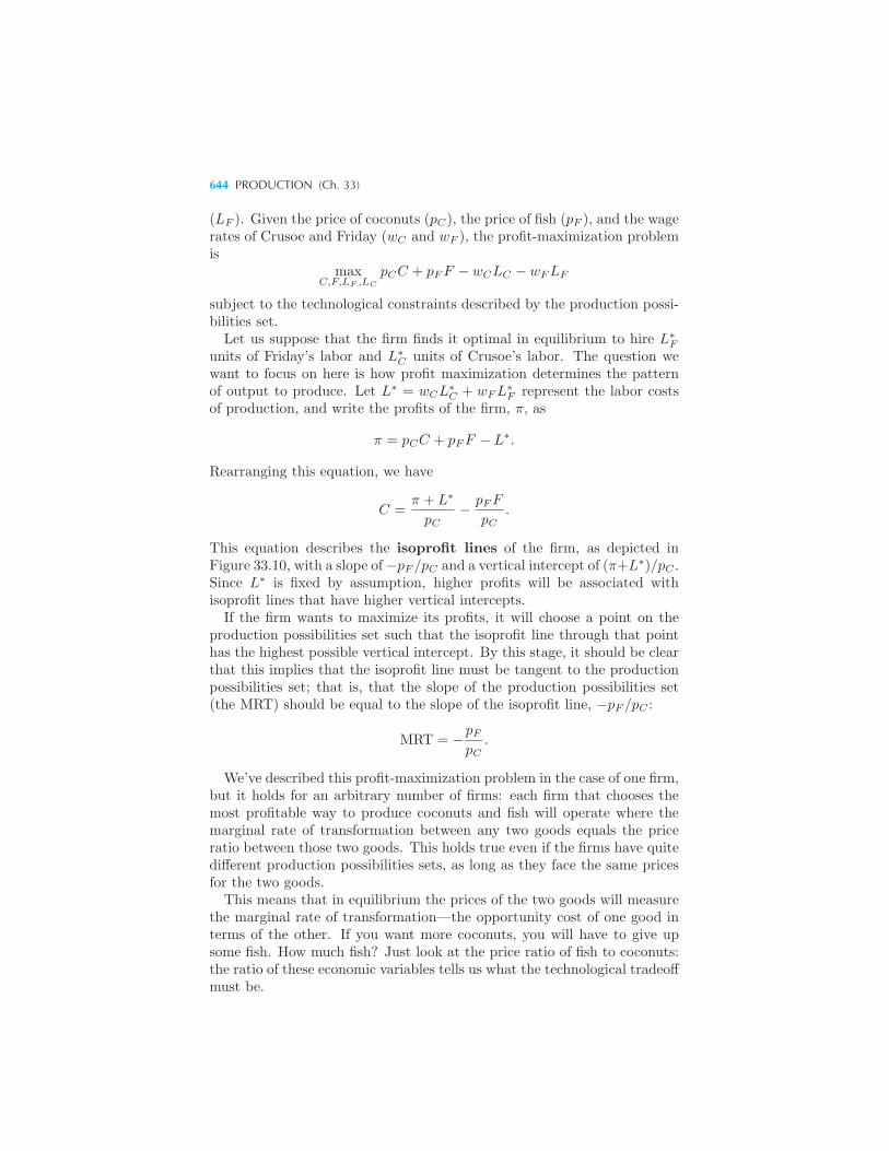
644 PRODUCTION (Ch. 33)
(LF ). Given the price of coconuts (pC), the price of fish (pF ), and the wagerates of Crusoe and Friday (wC and wF ), the profit-maximization problemis
maxC,F,LF ,LC
pCC + pFF − wCLC − wFLF
subject to the technological constraints described by the production possi-bilities set.Let us suppose that the firm finds it optimal in equilibrium to hire L∗
F
units of Friday’s labor and L∗C units of Crusoe’s labor. The question we
want to focus on here is how profit maximization determines the patternof output to produce. Let L∗ = wCL
∗C + wFL
∗F represent the labor costs
of production, and write the profits of the firm, π, as
π = pCC + pFF − L∗.
Rearranging this equation, we have
C =π + L∗
pC− pFF
pC.
This equation describes the isoprofit lines of the firm, as depicted inFigure 33.10, with a slope of−pF /pC and a vertical intercept of (π+L∗)/pC .Since L∗ is fixed by assumption, higher profits will be associated withisoprofit lines that have higher vertical intercepts.If the firm wants to maximize its profits, it will choose a point on the
production possibilities set such that the isoprofit line through that pointhas the highest possible vertical intercept. By this stage, it should be clearthat this implies that the isoprofit line must be tangent to the productionpossibilities set; that is, that the slope of the production possibilities set(the MRT) should be equal to the slope of the isoprofit line, −pF /pC :
MRT = −pFpC
.
We’ve described this profit-maximization problem in the case of one firm,but it holds for an arbitrary number of firms: each firm that chooses themost profitable way to produce coconuts and fish will operate where themarginal rate of transformation between any two goods equals the priceratio between those two goods. This holds true even if the firms have quitedifferent production possibilities sets, as long as they face the same pricesfor the two goods.This means that in equilibrium the prices of the two goods will measure
the marginal rate of transformation—the opportunity cost of one good interms of the other. If you want more coconuts, you will have to give upsome fish. How much fish? Just look at the price ratio of fish to coconuts:the ratio of these economic variables tells us what the technological tradeoffmust be.
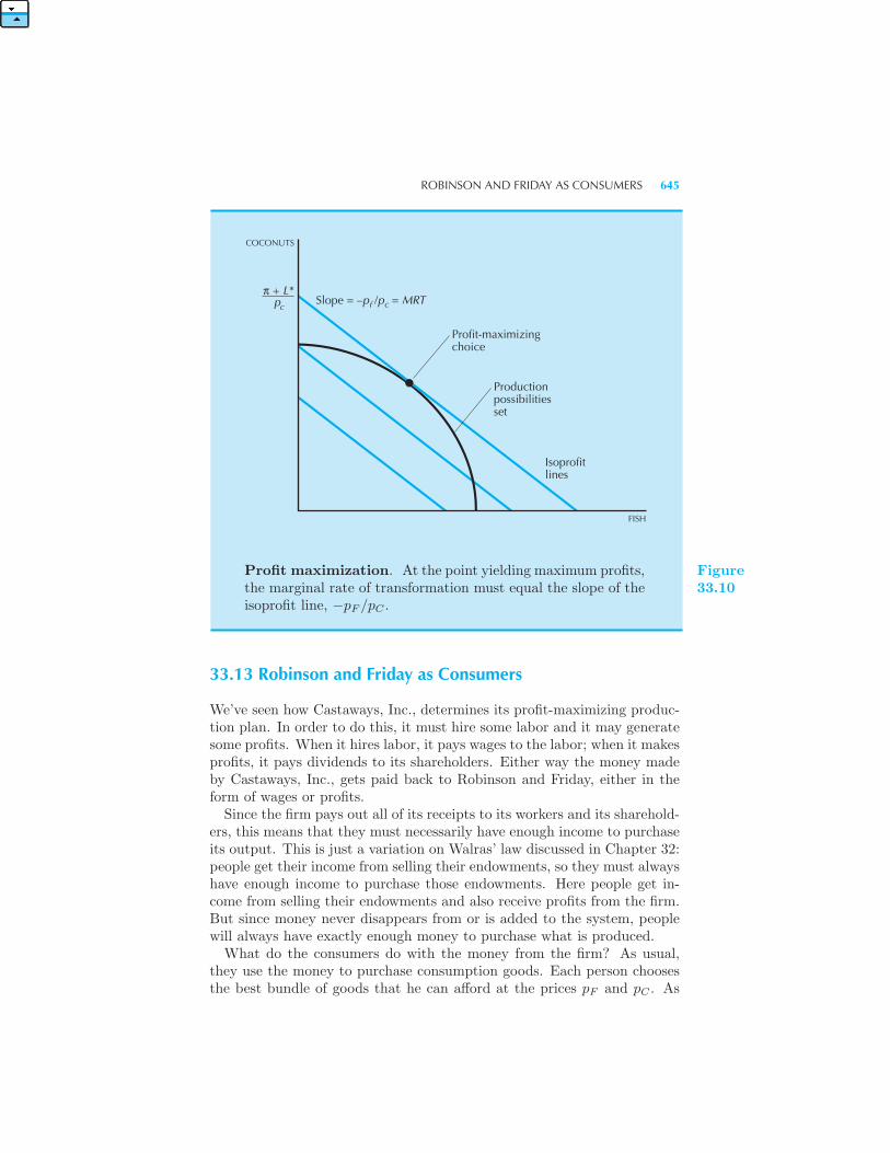
ROBINSON AND FRIDAY AS CONSUMERS 645
FISH
Productionpossibilitiesset
Profit-maximizingchoice
Slope = –p /p = MRT
COCONUTS
π + L*p f c
Isoprofitlines
c
Profit maximization. At the point yielding maximum profits,the marginal rate of transformation must equal the slope of theisoprofit line, −pF /pC .
Figure33.10
33.13 Robinson and Friday as Consumers
We’ve seen how Castaways, Inc., determines its profit-maximizing produc-tion plan. In order to do this, it must hire some labor and it may generatesome profits. When it hires labor, it pays wages to the labor; when it makesprofits, it pays dividends to its shareholders. Either way the money madeby Castaways, Inc., gets paid back to Robinson and Friday, either in theform of wages or profits.Since the firm pays out all of its receipts to its workers and its sharehold-
ers, this means that they must necessarily have enough income to purchaseits output. This is just a variation on Walras’ law discussed in Chapter 32:people get their income from selling their endowments, so they must alwayshave enough income to purchase those endowments. Here people get in-come from selling their endowments and also receive profits from the firm.But since money never disappears from or is added to the system, peoplewill always have exactly enough money to purchase what is produced.What do the consumers do with the money from the firm? As usual,
they use the money to purchase consumption goods. Each person choosesthe best bundle of goods that he can afford at the prices pF and pC . As
646 PRODUCTION (Ch. 33)
we’ve seen earlier, the optimal consumption bundle for each consumer mustsatisfy the condition that the marginal rate of substitution between the twogoods must be equal to the common price ratio. But this price ratio is alsoequal to the marginal rate of transformation, due to profit maximizationby the firm. Thus the necessary conditions for Pareto efficiency are met:the MRS of each consumer equals the MRT.In this economy, the prices of the goods serve as a signal of relative
scarcity. They indicate the technological scarcity—how much the produc-tion of one good must be reduced in order to produce more of the other;and they indicate the consumption scarcity—how much people are willingto reduce their consumption of one good in order to acquire some of theother good.
33.14 Decentralized Resource Allocation
The Crusoe-Friday economy is a drastically simplified picture. In orderto make a start on a larger model of the functioning of an economy, oneneeds to use substantially more elaborate mathematics. However, even thissimple model contains some useful insights.The most important of these is the relationship between individuals’
private goals of utility maximization and the social goals of efficient useof resources. Under certain conditions, the individuals’ pursuit of privategoals will result in an allocation that is Pareto efficient overall. Further-more, any Pareto efficient allocation can be supported as an outcome ofa competitive market, if initial endowments—including the ownership offirms—can be suitably redistributed.The great virtue of a competitive market is that each individual and each
firm only has to worry about its own maximization problem. The only factsthat need to be communicated among the firms and the consumers are theprices of the goods. Given these signals of relative scarcity, consumers andfirms have enough information to make decisions that achieve an efficientallocation of resources. In this sense, the social problems involved in effi-ciently utilizing resources can be decentralized, and solved at the individuallevel.Each individual can solve his or her own problem of what to consume.
The firms face the prices of the goods the consumers consume and decidehow much to produce of each of them. In making this decision, they areguided by profit signals. In this context, profits serve as exactly the rightguide. To say that a production plan is profitable is to say that peopleare willing to pay more for some good than it costs to produce it—so it isnatural to expand the production of such goods. If all firms pursue a com-petitive profit-maximizing policy, and all consumers choose consumptionbundles to maximize their own utility, then resulting competitive equilib-rium must be a Pareto efficient allocation.
REVIEW QUESTIONS 647
Summary
1. The general equilibrium framework can be extended by allowing com-petitive, profit-maximizing firms to produce goods destined for exchangein the economy.
2. Under certain conditions there exists a set of prices for all of the inputand output goods in the economy such that the profit-maximizing actionsof firms along with the utility-maximizing behavior of individuals resultsin the demand for each good equaling the supply in all markets—that is, acompetitive equilibrium exists.
3. Under certain conditions the resulting competitive equilibrium will bePareto efficient: the First Welfare Theorem holds in an economy with pro-duction.
4. With the addition of convex production sets, the Second Welfare Theo-rem also holds in the case of production.
5. When goods are being produced as efficiently as possible, the marginalrate of transformation between two goods indicates the number of units ofone good the economy must give up to obtain additional units of the othergood.
6. Pareto efficiency requires that each individual’s marginal rate of substi-tution be equal to the marginal rate of transformation.
7. The virtue of competitive markets is that they provide a way to achievean efficient allocation of resources by decentralizing production and con-sumption decisions.
REVIEW QUESTIONS
1. The competitive price of coconuts is $6 per pound and the price of fishis $3 per pound. If society were to give up 1 pound of coconuts, how manymore pounds of fish could be produced?
2. What would happen if the firm depicted in Figure 33.2 decided to pay ahigher wage?
3. In what sense is a competitive equilibrium a good or bad thing for agiven economy?
648 PRODUCTION (Ch. 33)
4. If Robinson’s marginal rate of substitution between coconuts and fish is−2 and the marginal rate of transformation between the two goods is −1,what should he do if he wants to increase his utility?
5. Suppose that Robinson and Friday both want 60 pounds of fish and60 pounds of coconuts per day. Using the production rates given in thechapter, how many hours must Robinson and Friday work per day if theydon’t help each other? Suppose they decide to work together in the mostefficient manner possible. Now how many hours each day do they have towork? What is the economic explanation for the reduction in hours?
APPENDIX
Let us derive the calculus conditions for Pareto efficiency in an economy withproduction. We let X1 and X2 represent the total amount of good 1 and good 2produced and consumed, as in the body of this chapter:
X1 = x1A + x1
B
X2 = x2A + x2
B .
The first thing we need is a convenient way to describe the production pos-sibilities frontier—all the combinations of X1 and X2 that are technologicallyfeasible. The most useful way to do this for our purposes is by use of the trans-formation function. This is a function of the aggregate amounts of the twogoods T (X1, X2), such that the combination (X1, X2) is on the production pos-sibilities frontier (the boundary of the production possibilities set) if and onlyif
T (X1, X2) = 0.
Once we have described the technology, we can calculate the marginal rateof transformation: the rate at which we have to sacrifice good 2 in order toproduce more of good 1. Although the name evokes an image of one good being“transformed” into another, that is a somewhat misleading picture. What reallyhappens is that other resources are moved from producing good 2 to producinggood 1. Thus, by devoting fewer resources to good 2 and more to good 1, wemove from one point on the production possibilities frontier to another. Themarginal rate of transformation is just the slope of the production possibilitiesset, which we denote by dX2/dX1.
Consider a small change in production (dX1, dX2) that remains feasible. Thuswe have
∂T (X1, X2)
∂X1dX1 +
∂T (X1, X2)
∂X2dX2 = 0.
Solving for the marginal rate of transformation:
dX2
dX1= −∂T/∂X1
∂T/∂X2.
APPENDIX 649
We’ll use this formula in a moment.A Pareto efficient allocation is one that maximizes any one person’s utility,
given the level of the other people’s utility. In the two-person case, we can writethis maximization problem as
maxx1A,x2
A,x1
B,x2
B
uA(x1A, x
2A)
such that uB(x1B , x
2B) = u
T (X1, X2) = 0.
The Lagrangian for this problem is
L = uA(x1A, x
2A)− λ(uB(x
1B , x
2B)− u)
− μ(T (X1, X2)− 0),
and the first-order conditions are
∂L
∂x1A
=∂uA
∂x1A
− μ∂T
∂X1= 0
∂L
∂x2A
=∂uA
∂x2A
− μ∂T
∂X2= 0
∂L
∂x1B
= −λ∂uB
∂x1B
− μ∂T
∂X1= 0
∂L
∂x2B
= −λ∂uB
∂x2B
− μ∂T
∂X2= 0.
Rearranging and dividing the first equation by the second gives
∂uA/∂x1A
∂uA/∂x2A
=∂T/∂X1
∂T/∂X2.
Performing the same operation on the third and fourth equations gives
∂uB/∂x1B
∂uB/∂x2B
=∂T/∂X1
∂T/∂X2.
The left-hand sides of these equations are our old friends, the marginal ratesof substitution. The right-hand side is the marginal rate of transformation. Thusthe equations require that each person’s marginal rate of substitution betweenthe goods must equal the marginal rate of transformation: the rate at which eachperson is just willing to substitute one good for the other must be the same as therate at which it is technologically feasible to transform one good into the other.
The intuition behind this result is straightforward. Suppose that the MRS forsome individual was not equal to the MRT. Then the rate at which the individualwould be willing to sacrifice one good to get more of the other would be differentthan the rate that was technologically feasible—but this means that there wouldbe some way to increase that individual’s utility while not affecting anyone else’sconsumption.

CHAPTER 34
WELFARE
Up until now we have focused on considerations of Pareto efficiency in eval-uating economic allocations. But there are other important considerations.It must be remembered that Pareto efficiency has nothing to say about thedistribution of welfare across people; giving everything to one person willtypically be Pareto efficient. But the rest of us might not consider this areasonable allocation. In this chapter we will investigate some techniquesthat can be used to formalize ideas related to the distribution of welfare.Pareto efficiency is in itself a desirable goal—if there is some way to make
some group of people better off without hurting other people, why not doit? But there will usually be many Pareto efficient allocations; how cansociety choose among them?The major focus of this chapter will be the idea of a welfare function,
which provides a way to “add together” different consumers’ utilities. Moregenerally, a welfare function provides a way to rank different distributionsof utility among consumers. Before we investigate the implications of thisconcept, it is worthwhile considering just how one might go about “addingtogether” the individual consumers’ preferences to construct some kind of“social preferences.”
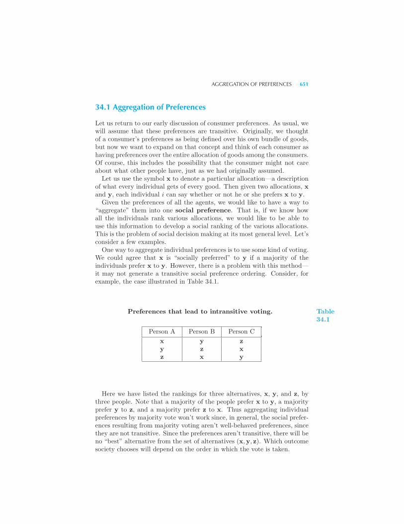
AGGREGATION OF PREFERENCES 651
34.1 Aggregation of Preferences
Let us return to our early discussion of consumer preferences. As usual, wewill assume that these preferences are transitive. Originally, we thoughtof a consumer’s preferences as being defined over his own bundle of goods,but now we want to expand on that concept and think of each consumer ashaving preferences over the entire allocation of goods among the consumers.Of course, this includes the possibility that the consumer might not careabout what other people have, just as we had originally assumed.Let us use the symbol x to denote a particular allocation—a description
of what every individual gets of every good. Then given two allocations, xand y, each individual i can say whether or not he or she prefers x to y.Given the preferences of all the agents, we would like to have a way to
“aggregate” them into one social preference. That is, if we know howall the individuals rank various allocations, we would like to be able touse this information to develop a social ranking of the various allocations.This is the problem of social decision making at its most general level. Let’sconsider a few examples.One way to aggregate individual preferences is to use some kind of voting.
We could agree that x is “socially preferred” to y if a majority of theindividuals prefer x to y. However, there is a problem with this method—it may not generate a transitive social preference ordering. Consider, forexample, the case illustrated in Table 34.1.
Preferences that lead to intransitive voting.
Person A Person B Person C
x y zy z xz x y
Table34.1
Here we have listed the rankings for three alternatives, x, y, and z, bythree people. Note that a majority of the people prefer x to y, a majorityprefer y to z, and a majority prefer z to x. Thus aggregating individualpreferences by majority vote won’t work since, in general, the social prefer-ences resulting from majority voting aren’t well-behaved preferences, sincethey are not transitive. Since the preferences aren’t transitive, there will beno “best” alternative from the set of alternatives (x,y, z). Which outcomesociety chooses will depend on the order in which the vote is taken.
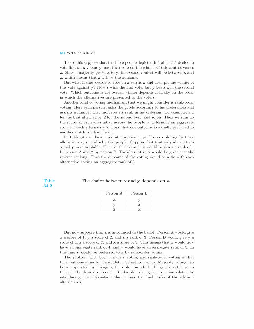
652 WELFARE (Ch. 34)
To see this suppose that the three people depicted in Table 34.1 decide tovote first on x versus y, and then vote on the winner of this contest versusz. Since a majority prefer x to y, the second contest will be between x andz, which means that z will be the outcome.
But what if they decide to vote on z versus x and then pit the winner ofthis vote against y? Now z wins the first vote, but y beats z in the secondvote. Which outcome is the overall winner depends crucially on the orderin which the alternatives are presented to the voters.Another kind of voting mechanism that we might consider is rank-order
voting. Here each person ranks the goods according to his preferences andassigns a number that indicates its rank in his ordering: for example, a 1for the best alternative, 2 for the second best, and so on. Then we sum upthe scores of each alternative across the people to determine an aggregatescore for each alternative and say that one outcome is socially preferred toanother if it has a lower score.In Table 34.2 we have illustrated a possible preference ordering for three
allocations x, y, and z by two people. Suppose first that only alternativesx and y were available. Then in this example x would be given a rank of 1by person A and 2 by person B. The alternative y would be given just thereverse ranking. Thus the outcome of the voting would be a tie with eachalternative having an aggregate rank of 3.
Table34.2
The choice between x and y depends on z.
Person A Person B
x yy zz x
But now suppose that z is introduced to the ballot. Person A would givex a score of 1, y a score of 2, and z a rank of 3. Person B would give y ascore of 1, z a score of 2, and x a score of 3. This means that x would nowhave an aggregate rank of 4, and y would have an aggregate rank of 3. Inthis case y would be preferred to x by rank-order voting.The problem with both majority voting and rank-order voting is that
their outcomes can be manipulated by astute agents. Majority voting canbe manipulated by changing the order on which things are voted so asto yield the desired outcome. Rank-order voting can be manipulated byintroducing new alternatives that change the final ranks of the relevantalternatives.
SOCIAL WELFARE FUNCTIONS 653
The question naturally arises as to whether there are social decisionmechanisms—ways of aggregating preferences—that are immune to thiskind of manipulation? Are there ways to “add up” preferences that don’thave the undesirable properties described above?Let’s list some things that we would want our social decision mechanism
to do:
1. Given any set of complete, reflexive, and transitive individual prefer-ences, the social decision mechanism should result in social preferencesthat satisfy the same properties.
2. If everybody prefers alternative x to alternative y, then the social pref-erences should rank x ahead of y.
3. The preferences between x and y should depend only on how people rankx versus y, and not on how they rank other alternatives.
All three of these requirements seem eminently plausible. Yet it canbe quite difficult to find a mechanism that satisfies all of them. In fact,Kenneth Arrow has proved the following remarkable result:1
Arrow’s Impossibility Theorem. If a social decision mechanism satis-fies properties 1, 2, and 3, then it must be a dictatorship: all social rankingsare the rankings of one individual.
Arrow’s Impossibility Theorem is quite surprising. It shows that threevery plausible and desirable features of a social decision mechanism areinconsistent with democracy: there is no “perfect” way to make socialdecisions. There is no perfect way to “aggregate” individual preferences tomake one social preference. If we want to find a way to aggregate individualpreferences to form social preferences, we will have to give up one of theproperties of a social decision mechanism described in Arrow’s theorem.
34.2 Social Welfare Functions
If we were to drop any of the desired features of a social welfare functiondescribed above, it would probably be property 3—that the social prefer-ence between two alternatives only depends on the ranking of those twoalternatives. If we do that, certain kinds of rank-order voting become pos-sibilities.
1 See Kenneth Arrow, Social Choice and Individual Values (New York: Wiley, 1963).Arrow, a professor at Stanford University, was awarded the Nobel Prize in economicsfor his work in this area.
654 WELFARE (Ch. 34)
Given the preferences of each individual i over the allocations, we canconstruct utility functions, ui(x), that summarize the individuals’ valuejudgments: person i prefers x to y if and only if ui(x) > ui(y). Of course,these are just like all utility functions—they can be scaled in any way thatpreserves the underlying preference ordering. There is no unique utilityrepresentation.But let us pick some utility representation and stick with it. Then one
way of getting social preferences from individuals’ preferences is to add upthe individual utilities and use the resulting number as a kind of social util-ity. That is, we will say that allocation x is socially preferred to allocationy if
n∑i=1
ui(x) >
n∑i=1
ui(y),
where n is the number of individuals in the society.This works—but of course it is totally arbitrary, since our choice of utility
representation is totally arbitrary. The choice of using the sum is alsoarbitrary. Why not use a weighted sum of utilities? Why not use theproduct of utilities, or the sum of the squares of utilities?One reasonable restriction that we might place on the “aggregating func-
tion” is that it be increasing in each individual’s utility. That way we areassured that if everybody prefers x to y, then the social preferences willprefer x to y.There is a name for this kind of aggregating function; it is called a social
welfare function. A social welfare function is just some function of theindividual utility functions: W (u1(x), . . . , un(x)). It gives a way to rankdifferent allocations that depends only on the individual preferences, andit is an increasing function of each individual’s utility.Let’s look at some examples. One special case mentioned above is the
sum of the individual utility functions
W (u1, . . . , un) =
n∑i=1
ui.
This is sometimes referred to as a classical utilitarian or Benthamitewelfare function.2 A slight generalization of this form is the weighted-sum-of-utilities welfare function:
W (u1, . . . , un) =n∑
i=1
aiui.
2 Jeremy Bentham (1748–1832) was the founder of the utilitarian school of moral phi-losophy, a school that considers the highest good to be the greatest happiness for thegreatest number.
WELFARE MAXIMIZATION 655
Here the weights, a1, . . . , an, are supposed to be numbers indicating howimportant each agent’s utility is to the overall social welfare. It is naturalto take each ai as being positive.Another interesting welfare function is the minimax or Rawlsian social
welfare function:
W (u1, . . . , un) = min{u1, . . . , un}.
This welfare function says that the social welfare of an allocation dependsonly on the welfare of the worst off agent—the person with the minimalutility.3
Each of these is a possible way to compare individual utility functions.Each of them represents different ethical judgments about the comparisonbetween different agents’ welfares. About the only restriction that we willplace on the structure of the welfare function at this point is that it beincreasing in each consumer’s utility.
34.3 Welfare Maximization
Once we have a welfare function we can examine the problem of welfaremaximization. Let us use the notation xj
i to indicate how much individuali has of good j, and suppose that there are n consumers and k goods. Thenthe allocation x consists of the list of how much each of the agents has ofeach of the goods.If we have a total amount X1, . . . , Xk of goods 1, . . . , k to distribute
among the consumers, we can pose the welfare maximization problem:
max W (u1(x), . . . , un(x))
such that
n∑i=1
x1i = X1
...n∑
i=1
xki = Xk.
Thus we are trying to find the feasible allocation that maximizes socialwelfare. What properties does such an allocation have?The first thing that we should note is that a maximal welfare allocation
must be a Pareto efficient allocation. The proof is easy: suppose that
3 John Rawls (1931–2002) was a philosopher at Harvard who has argued for this prin-ciple of justice.
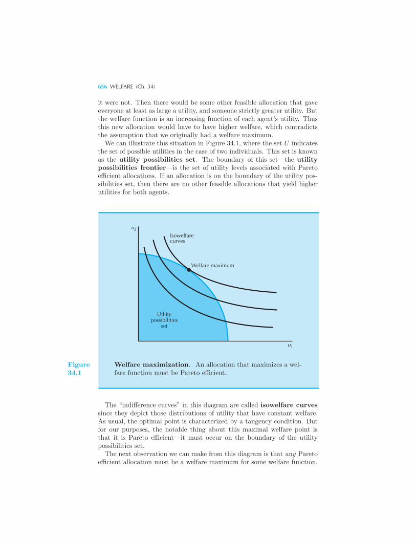
656 WELFARE (Ch. 34)
it were not. Then there would be some other feasible allocation that gaveeveryone at least as large a utility, and someone strictly greater utility. Butthe welfare function is an increasing function of each agent’s utility. Thusthis new allocation would have to have higher welfare, which contradictsthe assumption that we originally had a welfare maximum.We can illustrate this situation in Figure 34.1, where the set U indicates
the set of possible utilities in the case of two individuals. This set is knownas the utility possibilities set. The boundary of this set—the utilitypossibilities frontier—is the set of utility levels associated with Paretoefficient allocations. If an allocation is on the boundary of the utility pos-sibilities set, then there are no other feasible allocations that yield higherutilities for both agents.
Welfare maximum
Isowelfarecurves
u2
Utilitypossibilities
set
1u
Figure34.1
Welfare maximization. An allocation that maximizes a wel-fare function must be Pareto efficient.
The “indifference curves” in this diagram are called isowelfare curvessince they depict those distributions of utility that have constant welfare.As usual, the optimal point is characterized by a tangency condition. Butfor our purposes, the notable thing about this maximal welfare point isthat it is Pareto efficient—it must occur on the boundary of the utilitypossibilities set.The next observation we can make from this diagram is that any Pareto
efficient allocation must be a welfare maximum for some welfare function.
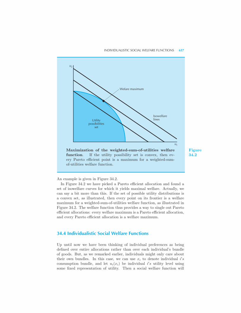
INDIVIDUALISTIC SOCIAL WELFARE FUNCTIONS 657
u1
Utilitypossibilities
set
u2
Wefare maximum
Isowelfarelines
Maximization of the weighted-sum-of-utilities welfarefunction. If the utility possibility set is convex, then ev-ery Pareto efficient point is a maximum for a weighted-sum-of-utilities welfare function.
Figure34.2
An example is given in Figure 34.2.
In Figure 34.2 we have picked a Pareto efficient allocation and found aset of isowelfare curves for which it yields maximal welfare. Actually, wecan say a bit more than this. If the set of possible utility distributions isa convex set, as illustrated, then every point on its frontier is a welfaremaximum for a weighted-sum-of-utilities welfare function, as illustrated inFigure 34.2. The welfare function thus provides a way to single out Paretoefficient allocations: every welfare maximum is a Pareto efficient allocation,and every Pareto efficient allocation is a welfare maximum.
34.4 Individualistic Social Welfare Functions
Up until now we have been thinking of individual preferences as beingdefined over entire allocations rather than over each individual’s bundleof goods. But, as we remarked earlier, individuals might only care abouttheir own bundles. In this case, we can use xi to denote individual i′sconsumption bundle, and let ui(xi) be individual i′s utility level usingsome fixed representation of utility. Then a social welfare function will
658 WELFARE (Ch. 34)
have the formW = W (u1(x1), . . . , un(xn)).
The welfare function is directly a function of the individuals’ utility levels,but it is indirectly a function of the individual agents’ consumption bun-dles. This special form of welfare function is known as an individualisticwelfare function or a Bergson-Samuelson welfare function.4
If each agent’s utility depends only on his or her own consumption, thenthere are no consumption externalities. Thus the standard results of Chap-ter 32 apply and we have an intimate relationship between Pareto efficientallocations and market equilibria: all competitive equilibria are Pareto ef-ficient, and, under appropriate convexity assumptions, all Pareto efficientallocations are competitive equilibria.Now we can carry this categorization one step further. Given the rela-
tionship between Pareto efficiency and welfare maxima described above, wecan conclude that all welfare maxima are competitive equilibria and thatall competitive equilibria are welfare maxima for some welfare function.
34.5 Fair Allocations
The welfare function approach is a very general way to describe socialwelfare. But because it is so general it can be used to summarize theproperties of many kinds of moral judgments. On the other hand, it isn’tmuch use in deciding what kinds of ethical judgments might be reasonableones.Another approach is to start with some specific moral judgments and
then examine their implications for economic distribution. This is theapproach taken in the study of fair allocations. We start with a definitionof what might be considered a fair way to divide a bundle of goods, and thenuse our understanding of economic analysis to investigate its implications.Suppose that you were given some goods to divide fairly among n equally
deserving people. How would you do it? It is probably safe to say thatin this problem most people would divide the goods equally among the nagents. Given that they are by hypothesis equally deserving, what elsecould you do?What is appealing about this idea of equal division? One appealing
feature is that it is symmetric. Each agent has the same bundle of goods;no agent prefers any other agent’s bundle of goods to his or her own, sincethey all have exactly the same thing.Unfortunately, an equal division will not necessarily be Pareto efficient.
If agents have different tastes they will generally desire to trade away from
4 Abram Bergson (1914–2002) and Paul Samuelson (1915–2009) were economists whoinvestigated properties of this kind of welfare function in the early 1940s. Samuelsonwas awarded a Nobel Prize in economics for his many contributions.
ENVY AND EQUITY 659
equal division. Let us suppose that this trade takes place and that it movesus to a Pareto efficient allocation.The question arises: is this Pareto efficient allocation still fair in any
sense? Does trade from equal division inherit any of the symmetry of thestarting point?The answer is: not necessarily. Consider the following example. We
have three people, A, B, and C. A and B have the same tastes, and C hasdifferent tastes. We start from an equal division and suppose that A andC get together and trade. Then they will typically both be made betteroff. Now B, who didn’t have the opportunity to trade with C, will envyA—that is, he would prefer A’s bundle to his own. Even though A andB started with the same allocation, A was luckier in her trading, and thisdestroyed the symmetry of the original allocation.This means that arbitrary trading from an equal division will not nec-
essarily preserve the symmetry of the starting point of equal division. Wemight well ask if there is any allocation that preserves this symmetry? Isthere any way to get an allocation that is both Pareto efficient and equitableat the same time?
34.6 Envy and Equity
Let us now try to formalize some of these ideas. What do we mean by“symmetric” or “equitable” anyway? One possible set of definitions is asfollows.We say an allocation is equitable if no agent prefers any other agent’s
bundle of goods to his or her own. If some agent i does prefer some otheragent j′s bundle of goods, we say that i envies j. Finally, if an allocationis both equitable and Pareto efficient, we will say that it is a fair allocation.These are ways of formalizing the idea of symmetry alluded to above. An
equal division allocation has the property that no agent envies any otheragent—but there are many other allocations that have this same property.Consider Figure 34.3. To determine whether any allocation is equitable
or not, just look at the allocation that results if the two agents swap bun-dles. If this swapped allocation lies “below” each agent’s indifference curvethrough the original allocation, then the original allocation is an equitableallocation. (Here “below” means below from the point of view of eachagent; from our point of view the swapped allocation must lie between thetwo indifference curves.)Note also that the allocation in Figure 34.3 is also Pareto efficient. Thus
it is not only equitable, in the sense that we defined the term, but it is alsoefficient. By our definition, it is a fair allocation. Is this kind of allocationa fluke, or will fair allocations typically exist?It turns out that fair allocations will generally exist, and there is an easy
way to see that this is so. We start as we did in the last section, where
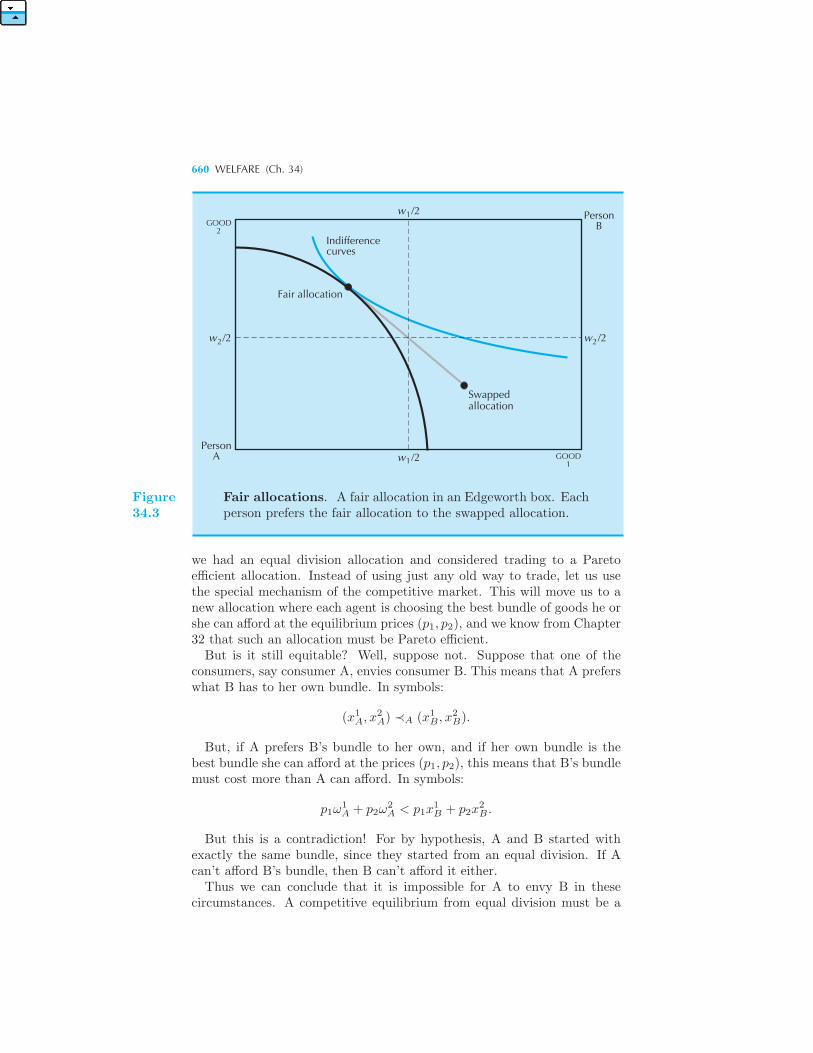
660 WELFARE (Ch. 34)
PersonA w /21 GOOD
1
PersonB
w /21GOOD
2Indifferencecurves
Fair allocation
w /22 2w /2
Swappedallocation
Figure34.3
Fair allocations. A fair allocation in an Edgeworth box. Eachperson prefers the fair allocation to the swapped allocation.
we had an equal division allocation and considered trading to a Paretoefficient allocation. Instead of using just any old way to trade, let us usethe special mechanism of the competitive market. This will move us to anew allocation where each agent is choosing the best bundle of goods he orshe can afford at the equilibrium prices (p1, p2), and we know from Chapter32 that such an allocation must be Pareto efficient.But is it still equitable? Well, suppose not. Suppose that one of the
consumers, say consumer A, envies consumer B. This means that A preferswhat B has to her own bundle. In symbols:
(x1A, x
2A) ≺A (x1
B , x2B).
But, if A prefers B’s bundle to her own, and if her own bundle is thebest bundle she can afford at the prices (p1, p2), this means that B’s bundlemust cost more than A can afford. In symbols:
p1ω1A + p2ω
2A < p1x
1B + p2x
2B .
But this is a contradiction! For by hypothesis, A and B started withexactly the same bundle, since they started from an equal division. If Acan’t afford B’s bundle, then B can’t afford it either.Thus we can conclude that it is impossible for A to envy B in these
circumstances. A competitive equilibrium from equal division must be a
REVIEW QUESTIONS 661
fair allocation. Thus the market mechanism will preserve certain kinds ofequity: if the original allocation is equally divided, the final allocation mustbe fair.
Summary
1. Arrow’s Impossibility Theorem shows that there is no ideal way to ag-gregate individual preferences into social preferences.
2. Nevertheless, economists often use welfare functions of one sort or an-other to represent distributional judgments about allocations.
3. As long as the welfare function is increasing in each individual’s utility,a welfare maximum will be Pareto efficient. Furthermore, every Paretoefficient allocation can be thought of as maximizing some welfare function.
4. The idea of fair allocations provides an alternative way to make distribu-tional judgments. This idea emphasizes the idea of symmetric treatment.
5. Even when the initial allocation is symmetric, arbitrary methods of tradewill not necessarily produce a fair allocation. However, it turns out thatthe market mechanism will provide a fair allocation.
REVIEW QUESTIONS
1. Suppose that we say that an allocation x is socially preferred to anallocation y only if everyone prefers x to y. (This is sometimes called thePareto ordering, since it is closely related to the idea of Pareto efficiency.)What shortcoming does this have as a rule for making social decisions?
2. A Rawlsian welfare function counts only the welfare of the worst offagent. The opposite of the Rawlsian welfare function might be called the“Nietzschean” welfare function—a welfare function that says the value ofan allocation depends only on the welfare of the best off agent. Whatmathematical form would the Nietzschean welfare function take?
3. Suppose that the utility possibilities set is a convex set and that con-sumers care only about their own consumption. What kind of allocationsrepresent welfare maxima of the Nietzschean welfare function?
4. Suppose that an allocation is Pareto efficient, and that each individualonly cares about his own consumption. Prove that there must be someindividual that envies no one, in the sense described in the text. (Thispuzzle requires some thought, but it is worth it.)
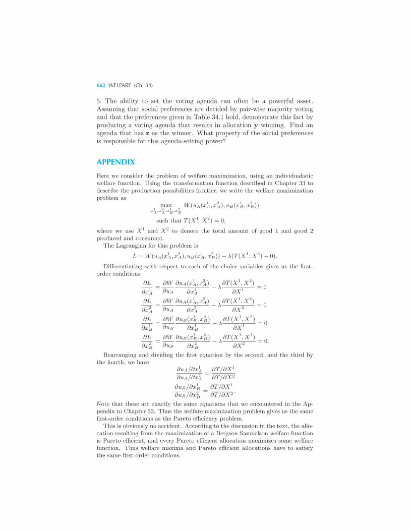
662 WELFARE (Ch. 34)
5. The ability to set the voting agenda can often be a powerful asset.Assuming that social preferences are decided by pair-wise majority votingand that the preferences given in Table 34.1 hold, demonstrate this fact byproducing a voting agenda that results in allocation y winning. Find anagenda that has z as the winner. What property of the social preferencesis responsible for this agenda-setting power?
APPENDIX
Here we consider the problem of welfare maximization, using an individualisticwelfare function. Using the transformation function described in Chapter 33 todescribe the production possibilities frontier, we write the welfare maximizationproblem as
maxx1A,x2
A,x1
B,x2
B
W (uA(x1A, x
2A), uB(x
1B , x
2B))
such that T (X1, X2) = 0,
where we use X1 and X2 to denote the total amount of good 1 and good 2produced and consumed.
The Lagrangian for this problem is
L = W (uA(x1A, x
2A), uB(x
1B , x
2B))− λ(T (X1, X2)− 0).
Differentiating with respect to each of the choice variables gives us the first-order conditions
∂L
∂x1A
=∂W
∂uA
∂uA(x1A, x
2A)
∂x1A
− λ∂T (X1, X2)
∂X1= 0
∂L
∂x2A
=∂W
∂uA
∂uA(x1A, x
2A)
∂x2A
− λ∂T (X1, X2)
∂X2= 0
∂L
∂x1B
=∂W
∂uB
∂uB(x1B , x
2B)
∂x1B
− λ∂T (X1, X2)
∂X1= 0
∂L
∂x2B
=∂W
∂uB
∂uB(x1B , x
2B)
∂x2B
− λ∂T (X1, X2)
∂X2= 0.
Rearranging and dividing the first equation by the second, and the third bythe fourth, we have
∂uA/∂x1A
∂uA/∂x2A
=∂T/∂X1
∂T/∂X2
∂uB/∂x1B
∂uB/∂x2B
=∂T/∂X1
∂T/∂X2.
Note that these are exactly the same equations that we encountered in the Ap-pendix to Chapter 33. Thus the welfare maximization problem gives us the samefirst-order conditions as the Pareto efficiency problem.
This is obviously no accident. According to the discussion in the text, the allo-cation resulting from the maximization of a Bergson-Samuelson welfare functionis Pareto efficient, and every Pareto efficient allocation maximizes some welfarefunction. Thus welfare maxima and Pareto efficient allocations have to satisfythe same first-order conditions.
CHAPTER 35
EXTERNALITIES
We say that an economic situation involves a consumption externality ifone consumer cares directly about another agent’s production or consump-tion. For example, I have definite preferences about my neighbor playingloud music at 3 in the morning, or the person next to me in a restaurantsmoking a cheap cigar, or the amount of pollution produced by local auto-mobiles. These are all examples of negative consumption externalities. Onthe other hand, I may get pleasure from observing my neighbor’s flowergarden—this is an example of a positive consumption externality.Similarly, a production externality arises when the production pos-
sibilities of one firm are influenced by the choices of another firm or con-sumer. A classic example is that of an apple orchard located next to abeekeeper, where there are mutual positive production externalities—eachfirm’s production positively affects the production possibilities of the otherfirm. Similarly, a fishery cares about the amount of pollutants dumpedinto its fishing area, since this will negatively influence its catch.The crucial feature of externalities is that there are goods people care
about that are not sold on markets. There is no market for loud music at 3in the morning, or drifting smoke from cheap cigars, or a neighbor who
664 EXTERNALITIES (Ch. 35)
keeps a beautiful flower garden. It is this lack of markets for externalitiesthat causes problems.
Up until now we have implicitly assumed that each agent could makeconsumption or production decisions without worrying about what otheragents were doing. All interactions between consumers and producers tookplace via the market, so that all the economic agents needed to know werethe market prices and their own consumption or production possibilities.In this chapter we will relax this assumption and examine the economicconsequences of externalities.
In earlier chapters we saw that the market mechanism was capable ofachieving Pareto efficient allocations when externalities were not present.If externalities are present, the market will not necessarily result in a Paretoefficient provision of resources. However, there are other social institutionssuch as the legal system, or government intervention, that can “mimic” themarket mechanism to some degree and thereby achieve Pareto efficiency.In this chapter we’ll see how these institutions work.
35.1 Smokers and Nonsmokers
It is convenient to start with an example to illustrate some of the mainconsiderations. We’ll imagine two roommates, A and B, who have prefer-ences over “money” and “smoke.” We suppose that both consumers likemoney, but that A likes to smoke and B likes clean air.
We can depict the consumption possibilities for the two consumers inan Edgeworth box. The length of the horizontal axis will represent thetotal amount of money the two agents have, and the height of the verticalaxis will represent the total amount of smoke that can be generated. Thepreferences of agent A are increasing in both money and smoke, whileagent B’s preferences are increasing in money and clean air—the absenceof smoke. We’ll measure smoke on a scale from 0 to 1, where 0 is no smokeat all, and 1 is the proverbial smoke-filled room.
This setup gives us a diagram like that depicted in Figure 35.1. Notethat the picture looks very much like the standard Edgeworth box, but theinterpretation is quite different. The amount of smoke is a good for A anda bad for B, so that B is moved to a more preferred position as A consumesless smoke. Be sure to note the difference in the way things are measuredon the horizontal and vertical axes. We measure A’s money horizontallyfrom the lower left-hand corner of the box, and B’s money horizontally fromthe upper right-hand corner. But the total amount of smoke is measuredvertically from the lower left-hand corner. The difference occurs becausemoney can be divided between the two consumers, so there will always betwo amounts of money to measure, but there is only one amount of smokethat they must both consume.
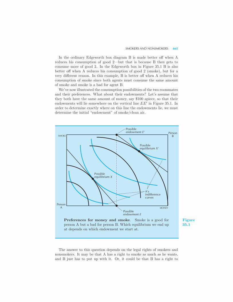
SMOKERS AND NONSMOKERS 665
In the ordinary Edgeworth box diagram B is made better off when Areduces his consumption of good 2—but that is because B then gets toconsume more of good 2. In the Edgeworth box in Figure 35.1 B is alsobetter off when A reduces his consumption of good 2 (smoke), but for avery different reason. In this example, B is better off when A reduces hisconsumption of smoke since both agents must consume the same amountof smoke and smoke is a bad for agent B.
We’ve now illustrated the consumption possibilities of the two roommatesand their preferences. What about their endowments? Let’s assume thatthey both have the same amount of money, say $100 apiece, so that theirendowments will lie somewhere on the vertical line EE′ in Figure 35.1. Inorder to determine exactly where on this line the endowments lie, we mustdetermine the initial “endowment” of smoke/clean air.
Possibleendowment E
Possibleendowment E'
Possible equilibrium X
Possible equilibrium X'
A'sindifferencecurves
MONEYPerson
A
SMOKEPerson
B
MONEY
Preferences for money and smoke. Smoke is a good forperson A but a bad for person B. Which equilibrium we end upat depends on which endowment we start at.
Figure35.1
The answer to this question depends on the legal rights of smokers andnonsmokers. It may be that A has a right to smoke as much as he wants,and B just has to put up with it. Or, it could be that B has a right to
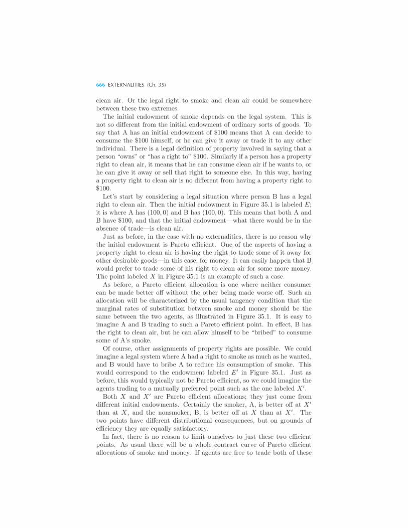
666 EXTERNALITIES (Ch. 35)
clean air. Or the legal right to smoke and clean air could be somewherebetween these two extremes.The initial endowment of smoke depends on the legal system. This is
not so different from the initial endowment of ordinary sorts of goods. Tosay that A has an initial endowment of $100 means that A can decide toconsume the $100 himself, or he can give it away or trade it to any otherindividual. There is a legal definition of property involved in saying that aperson “owns” or “has a right to” $100. Similarly if a person has a propertyright to clean air, it means that he can consume clean air if he wants to, orhe can give it away or sell that right to someone else. In this way, havinga property right to clean air is no different from having a property right to$100.Let’s start by considering a legal situation where person B has a legal
right to clean air. Then the initial endowment in Figure 35.1 is labeled E;it is where A has (100, 0) and B has (100, 0). This means that both A andB have $100, and that the initial endowment—what there would be in theabsence of trade—is clean air.Just as before, in the case with no externalities, there is no reason why
the initial endowment is Pareto efficient. One of the aspects of having aproperty right to clean air is having the right to trade some of it away forother desirable goods—in this case, for money. It can easily happen that Bwould prefer to trade some of his right to clean air for some more money.The point labeled X in Figure 35.1 is an example of such a case.As before, a Pareto efficient allocation is one where neither consumer
can be made better off without the other being made worse off. Such anallocation will be characterized by the usual tangency condition that themarginal rates of substitution between smoke and money should be thesame between the two agents, as illustrated in Figure 35.1. It is easy toimagine A and B trading to such a Pareto efficient point. In effect, B hasthe right to clean air, but he can allow himself to be “bribed” to consumesome of A’s smoke.Of course, other assignments of property rights are possible. We could
imagine a legal system where A had a right to smoke as much as he wanted,and B would have to bribe A to reduce his consumption of smoke. Thiswould correspond to the endowment labeled E′ in Figure 35.1. Just asbefore, this would typically not be Pareto efficient, so we could imagine theagents trading to a mutually preferred point such as the one labeled X ′.
Both X and X ′ are Pareto efficient allocations; they just come fromdifferent initial endowments. Certainly the smoker, A, is better off at X ′
than at X, and the nonsmoker, B, is better off at X than at X ′. Thetwo points have different distributional consequences, but on grounds ofefficiency they are equally satisfactory.In fact, there is no reason to limit ourselves to just these two efficient
points. As usual there will be a whole contract curve of Pareto efficientallocations of smoke and money. If agents are free to trade both of these
QUASILINEAR PREFERENCES AND THE COASE THEOREM 667
goods, we know that they will end up somewhere on this contract curve.The exact position will depend on their property rights involving smokeand money and on the precise mechanism that they use to trade.One mechanism that they could use to trade is the price mechanism.
Just as before we could imagine an auctioneer calling out prices and askinghow much each agent would be willing to buy at those prices. If the initialendowment point gave A the property rights to smoke, he could considerselling some of his smoking rights to B in exchange for B’s money. Similarly,if the property rights for clean air were given to B, he could sell some ofhis clean air to A.When the auctioneer manages to find a set of prices where supply equals
demand everything is fine: we have a nice Pareto efficient outcome. Ifthere is a market for smoke, a competitive equilibrium will be Pareto effi-cient. Furthermore, the competitive prices will measure the marginal rateof substitution between the two goods, just as in the standard case.This is just like the usual Edgeworth box analysis, but described in
a slightly different framework. As long as we have well-defined propertyrights in the good involving the externality—no matter who holds the prop-erty rights—the agents can trade from their initial endowment to a Paretoefficient allocation. If we want to set up a market in the externality toencourage trade, that will work as well.The only problem arises if the property rights are not well defined. If A
believes that he has the right to smoke and B believes that he has the rightto clean air, we have difficulties. The practical problems with externalitiesgenerally arise because of poorly defined property rights.My neighbor may believe that he has the right to play his trumpet at 3 in
the morning, and I may believe that I have the right to silence. A firm maybelieve that it has the right to dump pollutants into the atmosphere that Ibreathe, while I may believe that it doesn’t. Cases where property rights arepoorly defined can lead to an inefficient production of externalities—whichmeans that there would be ways to make both parties involved better off bychanging the production of externalities. If property rights are well defined,and mechanisms are in place to allow for negotiation between people, thenpeople can trade their rights to produce externalities in the same way thatthey trade rights to produce and consume ordinary goods.
35.2 Quasilinear Preferences and the Coase Theorem
We argued above that as long as property rights were well defined, tradebetween agents would result in an efficient allocation of the externality. Ingeneral, the amount of the externality that will be generated in the efficientsolution will depend on the assignment of property rights. In the case of thetwo roommates, the amount of smoke generated will depend on whetherthe smoker has the property rights or the nonsmoker has them.
668 EXTERNALITIES (Ch. 35)
But there is a special case where the outcome of the externality is inde-pendent of the assignment of property rights. If the agents’ preferences arequasilinear, then every efficient solution must have the same amount ofthe externality.
This case is illustrated in Figure 35.2 for the Edgeworth box case ofthe smoker versus the nonsmoker. Since the indifference curves are allhorizontal translates of each other, the locus of mutual tangencies—the setof Pareto efficient allocations—will be a horizontal line. This means thatthe amount of smoke is the same in every Pareto efficient allocation; onlythe dollar amounts held by the agents differ across the efficient allocations.
SMOKE
MONEY
A's indifference curves
Paretoefficientallocations
B's indifference curves
PersonB
PersonA
Figure35.2
Quasilinear preferences and the Coase theorem. If eachconsumer’s preferences are quasilinear, so that they are all hor-izontal translates of each other, the set of Pareto efficient allo-cations will be a horizontal line. Thus there will be a uniqueamount of the externality, in this case smoke, at each Paretoefficient allocation.
The result that under certain conditions the efficient amount of the goodinvolved in the externality is independent of the distribution of propertyrights is sometimes known as the Coase Theorem. However, it should beemphasized just how special these conditions are. The quasilinear prefer-ence assumption implies that the demands for the good causing the exter-
PRODUCTION EXTERNALITIES 669
nality doesn’t depend on the distribution of income. Therefore a realloca-tion of endowments doesn’t affect the efficient amount of the externalities.This is sometimes expressed by saying that the Coase theorem is valid ifthere are no “income effects.”1
In this case, the Pareto efficient allocations will involve a unique amountof the externality being generated. The different Pareto efficient allocationswill involve different amounts of money being held by the consumers; butthe amount of the externality—the amount of smoke—will be independentof the distribution of wealth.
35.3 Production Externalities
Let us now consider a situation involving production externalities. FirmS produces some amount of steel, s, and also produces a certain amountof pollution, x, which it dumps into a river. Firm F, a fishery, is locateddownstream and is adversely affected by S’s pollution.Suppose that firm S’s cost function is given by cs(s, x), where s is the
amount of steel produced and x is the amount of pollution produced. FirmF’s cost function is given by cf (f, x), where f indicates the production offish and x is the amount of pollution. Note that F’s costs of producing agiven amount of fish depend on the amount of pollution produced by thesteel firm. We will suppose that pollution increases the cost of providingfish Δcf/Δx > 0, and that pollution decreases the cost of steel production,Δcs/Δx ≤ 0. This last assumption says that increasing the amount ofpollution will decrease the cost of producing steel—that reducing pollutionwill increase the cost of steel production, at least over some range.The steel firm’s profit-maximization problem is
maxs,x
pss− cs(s, x)
and the fishery’s profit-maximization problem is
maxf
pff − cf (f, x).
Note that the steel mill gets to choose the amount of pollution that itgenerates, but the fishery must take the level of pollution as outside of itscontrol.
1 Ronald Coase is an emeritus professor at the University of Chicago Law School. Hisfamous paper, “The Problem of Social Costs,” The Journal of Law & Economics, 3(October 1960), has been given a variety of interpretations. Some authors suggestthat Coase only asserted that costless bargaining over externalities achieves a Paretoefficient outcome, not that the outcome will be independent of the assignment ofproperty rights. Coase received the 1991 Nobel Prize in Economics for this work.
670 EXTERNALITIES (Ch. 35)
The conditions characterizing profit maximization will be
ps =Δcs(s
∗, x∗)
Δs
0 =Δcs(s
∗, x∗)
Δx
for the steel firm and
pf =Δcf (f
∗, x∗)
Δf
for the fishery. These conditions say that at the profit-maximizing point,the price of each good—steel and pollution—should equal its marginal cost.In the case of the steel firm, one of its products is pollution, which, byassumption, has a zero price. So the condition determining the profit-maximizing supply of pollution says to produce pollution until the cost ofan extra unit is zero.
It is not hard to see the externality here: the fishery cares about theproduction of pollution but has no control over it. The steel firm looksonly at the cost of producing steel when it makes its profit-maximizingcalculation; it doesn’t consider the cost it imposes on the fishery. Theincrease in the cost of fishing associated with an increase in pollution ispart of the social cost of steel production, and it is being ignored by thesteel firm. In general, we expect that the steel firm will produce too muchpollution from a social point of view since it ignores the impact of thatpollution on the fishery.
What does a Pareto efficient production plan for steel and fish look like?There is an easy way to see what it should be. Suppose that the fisheryand the steel firm merged and formed one firm that produced both fishand steel (and possibly pollution). Then there is no externality! For aproduction externality only arises when one firm’s actions affect anotherfirm’s production possibilities. If there is only one firm, then it will take theinteractions between its different “divisions” into account when it choosesthe profit-maximizing production plan. We say that the externality hasbeen internalized by this reassignment of property rights. Before themerger, each firm had the right to produce whatever amount of steel or fishor pollution that it wanted, regardless of what the other firm did. Afterthe merger, the combined firm has the right to control the production ofboth the steel mill and the fishery.
The merged firm’s profit-maximization problem is
maxs,f,x
pss+ pff − cs(s, x)− cf (f, x),
PRODUCTION EXTERNALITIES 671
which yields optimality conditions of
ps =Δcs(s, x)
Δs
pf =Δcf (f , x)
Δf
0 =Δcs(s, x)
Δx+
Δcf (f , x)
Δx.
The crucial term is the last one. This shows that the merged firm willtake into account the effect of pollution on the marginal costs of boththe steel firm and the fishery. When the steel division decides how muchpollution to produce, it considers the effect of this action on the profits ofthe fish division; that is, it takes the social cost of its production plan intoaccount.What does this imply about the amount of pollution produced? When
the steel firm acted independently, the amount of pollution was determinedby the condition
Δcs(s∗, x∗)
Δx= 0. (35.1)
That is, the steel mill produced pollution until the marginal cost was zero:
MCS(s∗, x∗) = 0.
In the merged firm, the amount of pollution is determined by the condition
Δcs(s, x)
Δx+
Δcf (f , x)
Δx= 0. (35.2)
That is, the merged firm produces pollution until the sum of the marginalcost to the steel mill and the marginal cost to the fishery is zero. Thiscondition can also be written as
−Δcs(s, x)
Δx=
Δcf (f , x)
Δx> 0 (35.3)
or−MCS(s, x) = MCF (f , x).
In this latter expression MCF (f , x) is positive, since more pollution in-creases the cost of producing a given amount of fish. Hence the mergedfirm will want to produce where −MCS(s, x) is positive; that is, it willwant to produce less pollution than the independent steel firm. When thetrue social cost of the externality involved in the steel production is takeninto account, the optimal production of pollution will be reduced.When the steel firm considers minimizing its private costs of producing
steel, it produces where the marginal cost of extra pollution equals zero;
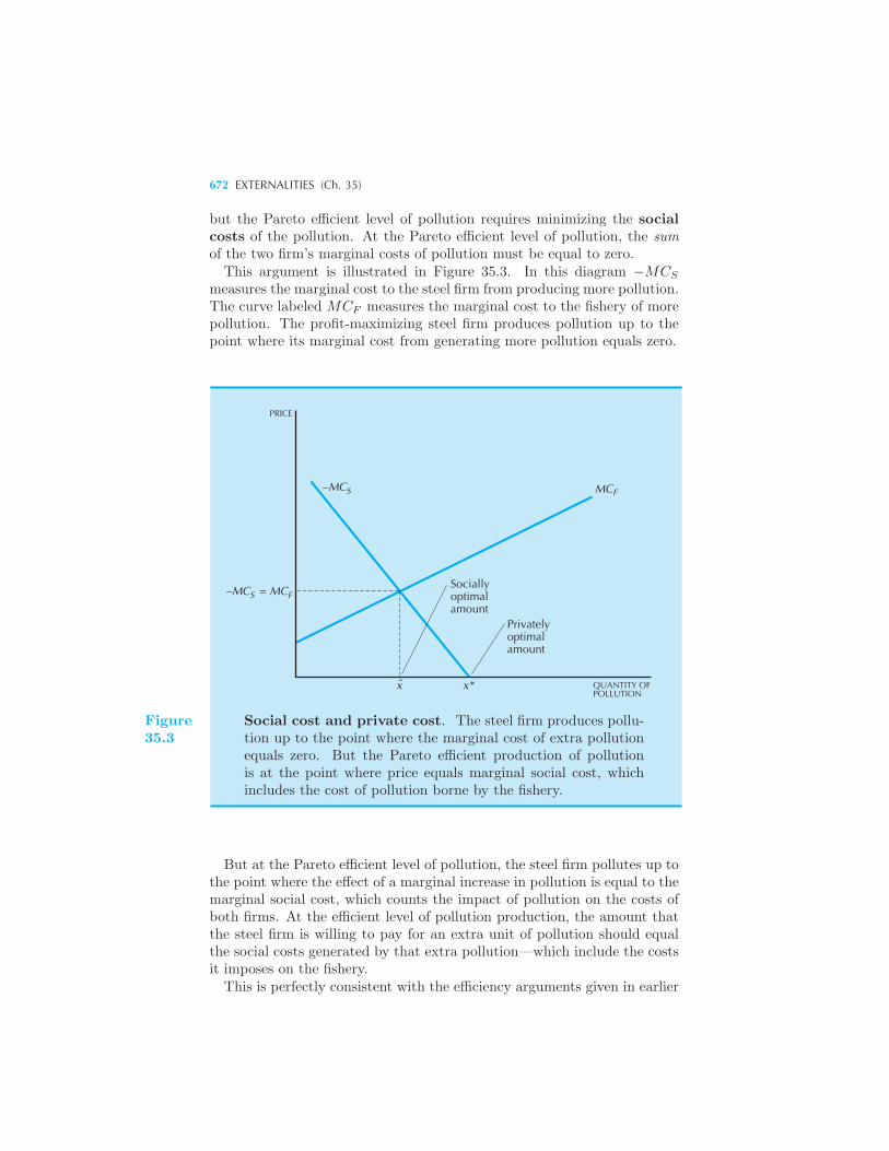
672 EXTERNALITIES (Ch. 35)
but the Pareto efficient level of pollution requires minimizing the socialcosts of the pollution. At the Pareto efficient level of pollution, the sumof the two firm’s marginal costs of pollution must be equal to zero.This argument is illustrated in Figure 35.3. In this diagram −MCS
measures the marginal cost to the steel firm from producing more pollution.The curve labeled MCF measures the marginal cost to the fishery of morepollution. The profit-maximizing steel firm produces pollution up to thepoint where its marginal cost from generating more pollution equals zero.
PRICE
–MC MC
–MC = MCS F
x x* QUANTITY OFPOLLUTION
Privatelyoptimalamount
Sociallyoptimalamount
S F
ˆ
Figure35.3
Social cost and private cost. The steel firm produces pollu-tion up to the point where the marginal cost of extra pollutionequals zero. But the Pareto efficient production of pollutionis at the point where price equals marginal social cost, whichincludes the cost of pollution borne by the fishery.
But at the Pareto efficient level of pollution, the steel firm pollutes up tothe point where the effect of a marginal increase in pollution is equal to themarginal social cost, which counts the impact of pollution on the costs ofboth firms. At the efficient level of pollution production, the amount thatthe steel firm is willing to pay for an extra unit of pollution should equalthe social costs generated by that extra pollution—which include the costsit imposes on the fishery.This is perfectly consistent with the efficiency arguments given in earlier
PRODUCTION EXTERNALITIES 673
chapters. There we assumed that there were no externalities, so that privatecosts and social costs coincided. In this case the free market will determinea Pareto efficient amount of output of each good. But if the private costsand the social costs diverge, the market alone may not be sufficient toachieve Pareto efficiency.
EXAMPLE: Pollution Vouchers
Everyone wants a clean environment . . . as long as someone else pays forit. Even if we reach a consensus on how much we should reduce pollution,there is still the problem of determining the most cost-effective way toachieve the targeted reduction.Take the case of nitrogen oxide emissions. One emitter may find it rela-
tively inexpensive to reduce its emissions of this pollutant, whereas anothermay find it very expensive. Should they both be required to reduce theiremission of pollutants by the same physical amount, by the same propor-tional amount, or by some other rule?Let’s look at a simple economic model. Suppose that there are only
two firms. Firm 1’s emission quota is x1 and firm 2’s is x2. The cost ofachieving an emission quota x1 is c1(x1) and similarly for firm 2. The totalamount of emission is fixed at some target level X. If we want to minimizethe total costs of achieving the emissions target, subject to the aggregateconstraint, we need to solve the following problem:
minx1,x2
c1(x1) + c2(x2)
such that x1 + x2 = X.
A by now standard economic argument shows that the marginal cost ofemission control must be equalized across the firms. If one firm had ahigher marginal cost of emission control than the other, then we couldlower total costs by reducing its quota and increasing the quota of theother firm.How can we achieve this outcome? If the government regulators had
information on the cost of emissions for all firms, they could calculate theappropriate pattern of production and impose it on all the relevant parties.But the cost of gathering all this information, and keeping it up-to-date, isstaggering. It is much easier to characterize the optimal solution than toactually implement it!Many economists have argued that the best way to implement the effi-
cient solution to the emission control problem is to use a market. It appearsthat such a market based emissions control system will soon be put intoeffect in Southern California. Here is how the California plan works.2
2 See Richard Stevenson, “Trying a Market Approach to Smog,” New York Times,March 25, 1992, C1.
674 EXTERNALITIES (Ch. 35)
Each of the 2700 largest polluters in Southern California is assigned aquota for their emissions of nitrogen oxide. This quota is initially set to be8 percent less than their previous year’s emission. If the firm exactly meetsits emissions quota it faces no fines or penalties. However, if it reduces itsemissions by more than its emissions quota, it can sell the extra “right toemit” on the open market.Suppose that a firm’s quota is 95 tons of nitrogen oxide emissions per
year. If it manages to produce only 90 tons in a given year, then it can sellthe right to emit 5 tons of nitrogen oxide to some other firm. Each firm cancompare the market price of an emission credit to the cost of reducing itsemissions and decide whether it was more cost-effective to reduce emissionsfurther or purchase emission credits from other firms.Firms that find it easy to reduce emissions will sell credits to firms that
find it costly to reduce emissions. In equilibrium, the market price of theright to emit one ton of pollution should just equal the marginal cost ofreducing emissions by one ton. But this is exactly the condition character-izing the optimal pattern of emissions! The market for emission permitsproduces the efficient pattern of emissions automatically.
35.4 Interpretation of the Conditions
There are several useful interpretations of the conditions for Pareto effi-ciency derived above. Each of these interpretations suggests a scheme tocorrect the efficiency loss created by the production externality.The first interpretation is that the steel firm faces the wrong price for
pollution. As far as the steel firm is concerned, its production of pollutioncosts it nothing. But that neglects the costs that the pollution imposeson the fishery. According to this view, the situation can be rectified bymaking sure that the polluter faces the correct social cost of its actions.One way to do this is to place a tax on the pollution generated by the
steel firm. Suppose that we put a tax of t dollars per unit of pollutiongenerated by the steel firm. Then the profit-maximization problem of thesteel firm becomes
maxs,x
pss− cs(s, x)− tx.
The profit-maximization conditions for this problem will be
ps −Δcs(s, x)
Δs= 0
−Δcs(s, x)
Δx− t = 0.
Comparing these conditions to equation (35.3), we see that setting
t =Δcf (f , x)
Δx
INTERPRETATION OF THE CONDITIONS 675
will make these conditions the same as the conditions characterizing thePareto efficient level of pollution.This kind of a tax is known as a Pigouvian tax.3 The problem with
Pigouvian taxes is that we need to know the optimal level of pollution inorder to impose the tax. But if we knew the optimal level of pollution wecould just tell the steel firm to produce exactly that much and not have tomess with this taxation scheme at all.Another interpretation of the problem is that there is a missing market—
the market for the pollutant. The externality problem arises because thepolluter faces a zero price for an output good that it produces, even thoughpeople would be willing to pay money to have that output level reduced.From a social point of view, the output of pollution should have a negativeprice.We could imagine a world where the fishery had the right to clean water,
but could sell the right to allow pollution. Let q be the price per unit ofpollution, and let x be the amount of pollution that the steel mill produces.Then the steel mill’s profit-maximization problem is
maxs,x
pss− qx− cs(s, x),
and the fishery’s profit-maximization problem is
maxf,x
pff + qx− cf (f, x).
The term qx enters with a negative sign in the profit expression for thesteel firm since it represents a cost—the steel firm must buy the right togenerate x units of pollution. But it enters with a positive sign in theexpression for the profits of the fishery, since the fishery gets revenue fromselling this right.The profit-maximization conditions are
ps =Δcs(s, x)
Δs(35.4)
q = −Δcs(s, x)
Δx(35.5)
pf =Δcf (f, x)
Δf(35.6)
q =Δcf (f, x)
Δx. (35.7)
3 Arthur Pigou (1877–1959), an economist at Cambridge University, suggested suchtaxes in his influential book The Economics of Welfare.
676 EXTERNALITIES (Ch. 35)
Thus each firm is facing the social marginal cost of each of its actionswhen it chooses how much pollution to buy or sell. If the price of pollutionis adjusted until the demand for pollution equals the supply of pollution,we will have an efficient equilibrium, just as with any other good.Note that at the optimal solution, equations (35.5) and (35.7) imply that
−Δcs(s, x)
Δx=
Δcf (f, x)
Δx.
This says that the marginal cost to the steel firm of reducing pollutionshould equal the marginal benefit to the fishery of that pollution reduction.If this condition were not satisfied, we couldn’t have the optimal level ofpollution. This is, of course, the same condition we encountered in equation(35.3).In analyzing this problem we have stated that the fishery had a right to
clean water and that the steel mill had to purchase the right to pollute.But we could have assigned the property rights in the opposite way: thesteel mill could have the right to pollute and the fishery would have to payto induce the steel mill to pollute less. Just as in the case of the smokerand nonsmoker, this would also give an efficient outcome. In fact, it wouldgive precisely the same outcome, since exactly the same equations wouldhave to be satisfied.To see this, we now suppose that the steel mill has the right to pollute
up to some amount x, say, but the fishery is willing to pay it to reduce itspollution. The profit-maximization problem for the steel mill is then
maxs,x
pss+ q(x− x)− cs(s, x).
Now the steel mill has two sources of income: it can sell steel, and it cansell pollution relief. The price equals marginal cost conditions become
ps −Δcs(s, x)
Δs= 0 (35.8)
−q − Δcs(s, x)
Δx= 0. (35.9)
The fishery’s maximization problem is now
maxf,x
pff − q(x− x)− cf (f, x),
which has optimality conditions
pf − Δcf (f, x)
Δf= 0 (35.10)
q − Δcf (f, x)
Δx= 0. (35.11)
MARKET SIGNALS 677
Now observe: the four equations (35.8)–(35.11) are precisely the same asthe four equations (35.4)–(35.7). In the case of production externalities, theoptimal pattern of production is independent of the assignment of propertyrights. Of course, the distribution of profits will generally depend on theassignment of property rights. Even though the social outcome will beindependent of the distribution of property rights, the owners of the firms inquestion may have strong views about what is an appropriate distribution.
35.5 Market Signals
Finally we turn to the third interpretation of externalities, which in somerespects is the most profound. In the case of the steel mill and the fisherythere is no problem if both firms merge—so why don’t they merge? In fact,when you think about it, there is a definite incentive for the two firms tomerge: if the actions of one affect the other, then they can make higherprofits together by coordinating their behavior than by each going alone.The objective of profit maximization itself should encourage the internal-ization of production externalities.Said another way: if the joint profits of the firms with coordination
exceed the sum of the profits without coordination, then the current ownerscould each be bought out for an amount equal to the present value of thestream of profits for their firm, the two firms could be coordinated, and thebuyer could retain the excess profits. The new buyer could be either of theold firms, or anybody else for that matter.The market itself provides a signal to internalize production externalities,
which is one reason this kind of production externality is rarely observed.Most firms have already internalized the externalities between units thataffect each other’s production. The case of the apple orchard and thebeekeeper mentioned earlier is a case in point. Here there would be anexternality if the two firms ignored their interaction . . . but why wouldthey be so foolish as to do so? It is more likely that one or both of thefirms would realize that more profits could be made by coordinating theiractivities, either by mutual agreement or by the sale of one of the firms tothe other. Indeed, it is very common for apple orchards to keep honey beesfor the purpose of fertilizing the trees. That particular externality is easilyinternalized.
EXAMPLE: Bees and Almonds
Many varieties of fruit and nut trees need bees to pollinate their blossoms,thereby allowing the trees to produce crops.According to the Carl Hayden Bee Research Center in Tucson, Arizona,
honeybees pollinate about one-third of the human diet and more than 50
678 EXTERNALITIES (Ch. 35)
different agricultural crops valued at more than $20 billion a year in theUnited States.4
Some owners of orchards keep their own bees; some rely on their neigh-bors’ bees or wild bees. However, as the theory of externalities suggests,the most natural solution to the problem of inadequate bee supply is amarket for bee services.
Consider, for example, the California almond market. There are 530,000acres of almond trees in California, and every year, more than 1 millionhoneybee hives are needed to pollinate the trees. But California only has440,000 resident bee hives. There aren’t enough California bees to pollinateall those almond trees!
The solution is to import bees from other nearby states. There is, infact, a ready market for such services, with beekeepers bringing hives fromNorth Dakota, Washington, and Colorado to supplement the native Cali-fornia bees. The almond growers pay well for these services: in 2004, beepollination services sold for $54 per hive.
35.6 The Tragedy of the Commons
We have argued above that if property rights are well defined, there will beno problem with production externalities. But if property rights are notwell defined, the outcome of the economic interactions will undoubtedlyinvolve inefficiencies.
In this section we will examine a particularly well-known inefficiencycalled “the tragedy of the commons.”5 We will pose this problem in theoriginal context of a common grazing land, although there are many otherpossible illustrations.
Consider an agricultural village in which the villagers graze their cowson a common field. We want to compare two allocation mechanisms: thefirst is the private ownership solution where someone owns the field anddecides how many cows should graze there; the second is the solution wherethe field is owned in common by the villagers and access to it is free andunrestricted.
Suppose that it costs a dollars to buy a cow. How much milk the cowproduces will depend on how many other cows are grazed on the commonland. We’ll let f(c) be the value of the milk produced if there are c cowsgrazed on the common. Thus the value of the milk per cow is just theaverage product, f(c)/c.
4 Anna Oberthur, “Almond Growers Face Need for Bees,” Associated Press, February29, 2004.
5 See G. Hardin, “The Tragedy of the Commons,” Science, 1968, 1243–47.
THE TRAGEDY OF THE COMMONS 679
How many cows would be grazed on the common if we wanted to maxi-mize the total wealth of the village? In order to maximize the total amountof wealth, we set up the following problem:
maxc
f(c)− ac.
It should be clear by now that the maximal production will occur whenthe marginal product of a cow equals its cost, a:
MP (c∗) = a.
If the marginal product of a cow were greater than a, it would pay to putanother cow on the commons; and if it were less than a, it would pay totake one off.If the common grazing ground were owned by someone who could restrict
access to it, this is indeed the solution that would result. For in this case,the owner of the grazing grounds would purchase just the right amount ofcows to maximize his profits.Now what would happen if the individual villagers decided whether or
not to use the common field? Each villager has a choice of grazing a cowor not grazing one, and it will be profitable to graze a cow as long as theoutput generated by the cow is greater than the cost of a cow. Suppose thatthere are c cows currently being grazed, so that the current output per cowis f(c)/c. When a villager contemplates adding a cow, the total output willbe f(c+ 1), and the total number of cows will be c+ 1. Thus the revenuethat the cow generates for the villager will be f(c + 1)/(c + 1). He mustcompare this revenue to the cost of the cow, a. If f(c + 1)/(c + 1) > a, itis profitable to add the cow since the value of the output exceeds the cost.Hence the villagers will choose to graze cows until the average product ofa cow is driven to a. It follows that the total number of cows grazed willbe c, where
f(c)
c= a.
Another way to derive this result is to appeal to free entry. If it isprofitable to graze a cow on the common field, villagers will purchase cows.They will stop adding cows to the common only when the profits have beendriven to zero, that is, when
f(c)− ac = 0,
which is just a rearrangement of the condition in the last paragraph.When an individual decides whether or not to purchase a cow, he looks
at the extra value he will get f(c)/c and compares this to the cost of thecow, a. This is fine for him, but what has been left out of this calculation isthe fact that his extra cow will reduce the output of milk from all the other
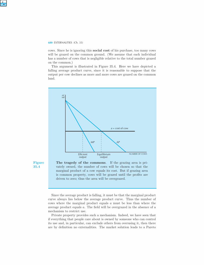
680 EXTERNALITIES (Ch. 35)
cows. Since he is ignoring this social cost of his purchase, too many cowswill be grazed on the common ground. (We assume that each individualhas a number of cows that is negligible relative to the total number grazedon the common.)This argument is illustrated in Figure 35.4. Here we have depicted a
falling average product curve, since it is reasonable to suppose that theoutput per cow declines as more and more cows are grazed on the commonland.
APMP
a = cost of cow
MP AP
Efficientoutput
Equilibriumoutput
NUMBER OF COWS
Figure35.4
The tragedy of the commons. If the grazing area is pri-vately owned, the number of cows will be chosen so that themarginal product of a cow equals its cost. But if grazing areais common property, cows will be grazed until the profits aredriven to zero; thus the area will be overgrazed.
Since the average product is falling, it must be that the marginal productcurve always lies below the average product curve. Thus the number ofcows where the marginal product equals a must be less than where theaverage product equals a. The field will be overgrazed in the absence of amechanism to restrict use.Private property provides such a mechanism. Indeed, we have seen that
if everything that people care about is owned by someone who can controlits use and, in particular, can exclude others from overusing it, then thereare by definition no externalities. The market solution leads to a Pareto
THE TRAGEDY OF THE COMMONS 681
efficient outcome. Inefficiencies can only result from situations where thereis no way to exclude others from using something, a topic that we willinvestigate in the next chapter.Of course, private property is not the only social institution that can
encourage efficient use of resources. For example, rules could be formulatedabout how many cows can be grazed on the village common. If there is alegal system to enforce those rules, this may be a cost-effective solution toproviding an efficient use of the common resource. However, in situationswhere the law is ambiguous or nonexistent, the tragedy of the commonscan easily arise. Overfishing in international waters and the exterminationof several species of animals due to overhunting are sobering examples ofthis phenomenon.
EXAMPLE: Overfishing
According to a report in the New York Times, “. . . overfishing has deci-mated the stocks of cod, haddock and flounder that have sustained NewEnglanders for centuries.”6 According to one expert, fishermen in NewEngland are taking 50 to 70 percent of the available stock, over twice thesustainable amount.This overfishing is a prime example of the problem of the commons:
each fisherman has a negligible impact on the total stock of fish, but theaccumulated efforts of thousands of fishermen results in serious depletion.The New England Fisheries Management Council is attempting to alleviatethe problem by banning new entry to the industry, requiring fishermen tolimit their days at sea, and increasing the mesh size of their nets.It appears that the supplies of fish could be restocked in as little as 5
years if conservation measures were undertaken. The present value of prof-its to the industry as a whole would be larger with regulation to preventoverfishing. However, such measures would almost certainly imply a sub-stantial reduction in the number of fishing boats in the industry, which ishighly unpopular with the small fishermen, who would likely be forced toleave the industry.
EXAMPLE: New England Lobsters
Some fishing industries have already applied stringent rules to avoid over-fishing. For example, lobster fishermen work under carefully designed rulesto ensure that they do not fish themselves out of a livelihood. For example,they are required to toss back any female lobster bearing eggs, any lobster
6 “Plenty of Fish in the Sea? Not Anymore,” New York Times, March 25, 1992, A15.
682 EXTERNALITIES (Ch. 35)
shorter than a minimum size, and any lobsters bigger than a maximumsize.The “eggers” give birth to more lobsters and the small “tiddlers” grow
up to mate. But why throw back the big lobsters? According to marinebiologists, large lobsters produce more offspring and larger offspring. Iffishermen always took the largest lobsters, the remaining small lobsterswould pass their genes onto their progeny, resulting in smaller and smallerlobsters in each generation.With lobsters there is good news and bad news. First the good news.
The 2003 Maine lobster harvest was 5.4 million pounds, more than 2.5 timesthe 1945–85 average. This suggests that the careful husbandry practicedby the industry has yielded a significant growth in the lobster population.However, it appears that conservation isn’t the only factor. There have
also been considerable changes in the population of other species of marinelife off the Maine coast, such as sea urchins, and some observers believe thatthese changes are the primary driver of change in the lobster population.7
This leads to the bad news. Further south, in Massachusetts and NewYork, the lobster catch has fallen dramatically. No one is quite sure whyone region is doing so well and the other so poorly. Ironically, Maine maybe doing well due to increased harvesting of finned fish and of sea urchins,both of which eat young lobsters. Massachusetts’ problems may be dueto specific factors, such as a large oil spill and a disfiguring shell disease.Another culprit is warming water: Narragansett Bay temperatures haverisen almost two degrees Celsius in the last 20 years.Ecologies can be very complex and can change rapidly. The efforts to
avoid overfishing are to be applauded, but they are only part of the story.
35.7 Automobile Pollution
As suggested above, pollution is a prime example of an economic external-ity. The activity of one consumer operating an automobile will typicallylower the quality of the air that other consumers breathe. It seems unlikelythat an unregulated free market would generate the optimal amount of pol-lution; more likely, if the consumer bears no cost in generating pollution,too much pollution would be produced.One approach to controlling the amount of automobile pollution is to re-
quire that automobiles meet certain standards in the amount of pollutionthat they generate. This has been the basic thrust of U.S. antipollutionpolicy since the Clean Air Act of 1963. That act, or, more properly, thesubsequent amendments, set automobile emission standards for the manu-facturers of vehicles in the United States.
7 See The Economist, “Claws!” August 19, 2004, and Cornelia Dean, “Lobster Boomand Bust,” New York Times, August 9, 2004.
AUTOMOBILE POLLUTION 683
Lawrence White has examined the benefits and costs of this program;most of the following discussion is drawn from this work.8
White estimates that the cost of emission control equipment is about$600 per car, the extra maintenance costs are about $180 per car, andthe costs of the reduced gasoline mileage and the necessity for unleadedgasoline come to about $670 per car. Thus the total cost per car of theemission control standards is about $1450 over the lifetime of the car. (Allfigures are in 1981 dollars.)He argues that there are several problems with the current approach to
the regulation of automobile emissions. First, it requires that all automo-biles meet the same standards. (California is the only state with differentstandards for emission control.) This means that everyone who buys a carmust pay an extra $1450 whether they live in a high pollution area or not.A 1974 National Academy of Sciences study concluded that 63 percent ofall U.S. cars did not require the stringent standards now in effect. Accord-ing to White, “almost two-thirds of car buyers are spending . . . substantialsums for unnecessary systems.”Secondly, most of the responsibility for meeting the standards falls on
the manufacturer, and little falls on the user. Owners of cars have littleincentive to keep their pollution control equipment in working order unlessthey live in a state with required inspections.More significantly, motorists have no incentive to economize on their
driving. In cities such as Los Angeles, where pollution is a significanthazard, it makes good economic sense to encourage people to drive less.Under the current system, people who drive 2000 miles a year in NorthDakota pay exactly the same amount for pollution control as people whodrive 50,000 miles a year in Los Angeles.An alternative solution to pollution would be effluent fees. As described
by White, effluent fees would require an annual inspection of all vehiclesalong with an odometer reading and tests that would estimate the likelyemissions of the vehicle during the past year. Different communities couldthen levy fees based on the estimated amount of pollution that had actu-ally been generated by the operation of the vehicle. This method wouldensure that people would face the true cost of generating pollution andwould encourage them to choose to generate the socially optimal amountof pollution.Such a system of effluent fees would encourage the vehicle owners them-
selves to find low-cost ways of reducing their emissions—investing in pol-lution control equipment, changing their driving habits, and changing thekinds of vehicles that they operate. A system of effluent fees could im-pose even higher standards than are now in effect in communities wherepollution is a serious problem. Any desired level of pollution control can
8 See Lawrence White, The Regulation of Air Pollutant Emissions from Motor Vehicles(Washington, D.C.: American Enterprise Institute for Public Policy Research, 1982).
684 EXTERNALITIES (Ch. 35)
be achieved by appropriate effluent fees . . . and it can be achieved at asubstantially lower cost than the current system of mandated standards.Of course, there is no reason why there might not also be some federally
mandated standards for the two-thirds of the vehicles that are operated inlocalities where pollution is not a serious problem. If it is cheaper to imposestandards than to require inspections, then by all means that should be theproper choice. The appropriate method of pollution control for automobilesshould depend on a rational analysis of benefits and costs—as should allsocial policies of this nature.
Summary
1. The First Theorem of Welfare Economics shows that a free, competitivemarket will provide an efficient outcome in the absence of externalities.
2. However, if externalities are present, the outcome of a competitive mar-ket is unlikely to be Pareto efficient.
3. However, in this case, the state can sometimes “mimic” the role of themarket by using prices to provide correct signals about the social cost ofindividual actions.
4. More importantly, the legal system can ensure that property rights arewell defined, so that efficiency-enhancing trades can be made.
5. If preferences are quasilinear, the efficient amount of a consumptionexternality will be independent of the assignment of property rights.
6. Cures for production externalities include the use of Pigouvian taxes,setting up a market for the externality, simply allowing firms to merge, ortransferring property rights in other ways.
7. The tragedy of the commons refers to the tendency for common propertyto be overused. This is a particularly prevalent form of externality.
REVIEW QUESTIONS
1. True or false? An explicit delineation of property rights usually elimi-nates the problem of externalities.
2. True or false? The distributional consequences of the delineation ofproperty rights are eliminated when preferences are quasilinear.
REVIEW QUESTIONS 685
3. List some other examples of positive and negative consumption andproduction externalities.
4. Suppose that the government wants to control the use of the commons,what methods exist for achieving the efficient level of use?

CHAPTER 36
INFORMATIONTECHNOLOGY
One of the most radical changes in the economy in the last 15 years hasbeen the emergence of the information economy. The popular press isfilled with stories about advances in computer technology, the Internet, andnew software. Not surprisingly, many of these stories are on the businesspages of the newspaper, for this technological revolution is also an economicrevolution.Some observers have gone so far as to put the Information Revolution
on a par with the Industrial Revolution. Just as the Industrial Revolutiontransformed the way goods were produced, distributed, and consumed, theInformation Revolution is transforming the way information is produced,distributed, and consumed.It has been claimed that these dramatically new technologies will require
a fundamentally different form of economics. Bits, it is argued, are fun-damentally different than atoms. Bits can be reproduced costlessly anddistributed around the world at the speed of light, and they never deterio-rate. Material goods, made of atoms, have none of these properties: theyare costly to produce and transport, and they inevitably deteriorate.It is true that the unusual properties of bits require new economic anal-
ysis, but I would argue that they do not require a new kind of economic
THE PROBLEM OF COMPLEMENTS 687
analysis. After all, economics is primarily about people not goods. Themodels we have analyzed in this book have had to do with how peoplemake choices and interact with each other. We have rarely had occasionto refer to the specific goods that were involved in the transactions. Thefundamental concerns were the tastes of the individuals, the technology ofproduction, and the structure of the market, and these same factors willdetermine how markets for information will work . . . or not work.In this chapter we will investigate a few economic models relevant to the
information revolution. The first has to do with the economics of networks,the second with switching costs, and the third with rights management forinformation goods. These examples will illustrate how the fundamentaltools of economic analysis can help us to understand the world of bits aswell as the world of atoms.
36.1 Systems Competition
Information technology is generally used in systems. Such systems involveseveral components, often provided by different firms, that only have valueif they work together. Hardware is useless without software, a DVD playeris useless without DVD disks, an operating system is worthless withoutapplications, and a web browser is useless without web servers. All of theseare examples of complements: goods where the value of one componentis significantly enhanced by the presence of another component.In our discussion of consumer theory, we described left shoes and right
shoes as complements. The cases above are equally extreme: the bestcomputer hardware in the world can’t function unless there is softwarewritten for it. But unlike shoes, the more software that is available for it,the more valuable it becomes.Competition among the providers of these components often have to
worry just as much about their “complementors” as their competitors.A key part of Apple’s competitive strategy has to involve their relationswith software developers. This gives competitive strategy in informationtechnology (IT) industries a different flavor than strategy in traditionalindustries.1
36.2 The Problem of Complements
To illustrate these points, let us consider the case of a Central Process-ing Unit (CPU) and an Operating System (OS). A CPU is an integrated
1 See Shapiro, Carl and Hal R. Varian, Information Rules: A Strategic Guide to theNetwork Economy, Harvard Business School Press, 1998, for a guide to competitivestrategy in IT industries.
688 INFORMATION TECHNOLOGY (Ch. 36)
circuit that is the “brain” of a computer. Two familiar manufacturers ofCPUs are Intel and Motorola. An OS is the software that allows usersand applications to access the functions of the CPU. Apple and Microsoftboth make operating systems. Normally, a special version of an operatingsystem has to be created for each CPU.From the viewpoint of the end user, the CPU can only be used if there
is a compatible operating system. The CPU and the OS are complements,just as left shoes and right shoes are complements.The most popular CPUs and OSs in the world today are made by Intel
and Microsoft, respectively. These are, of course, two separate companiesthat set the prices of their products independently. The PowerPC, anotherpopular CPU, was designed by a consortium consisting of IBM, Motorola,and Apple. Two commercial operating systems for the PowerPC are theApple OS and IBM’s AIX. In addition to these commercial operating sys-tems, there are free systems like BSD and GNU-Linux that are providedby groups of programmers working on a volunteer basis.Let us consider the pricing problem facing sellers of complementary prod-
ucts. The critical feature is that the demand for either product dependson the price of both products. If p1 is the price of the CPU and p2 is theprice of the OS, the cost to the end user depends on p1 + p2. Of course,you need more than just a CPU and an OS to make a useful system, butthat just adds more prices to the sum; we’ll keep things simple by stickingwith two components.The demand for CPUs depends on the price of the total system, so we
write D(p1+p2). If we let c1 be the marginal cost of a CPU and F the fixedcost, the profit-maximization problem of the CPU maker can be written
maxp1
(p1 − c1)D(p1 + p2)− F1.
Similarly, the profit-maximization problem of the OS maker can be written
maxp2
(p2 − c2)D(p1 + p2)− F2.
In order to analyze this problem, let us assume that the demand functionhas the linear form
D(p) = a− bp.
Let us also assume, for simplicity, that the marginal costs are so small thatthey can be ignored. Then the CPU profit-maximization problem becomes
maxp1
p1[a− b(p1 + p2)]− F1,
ormaxp1
ap1 − bp21 − bp1p2 − F1.
THE PROBLEM OF COMPLEMENTS 689
It turns out that the marginal revenue from a price increase Δp1 is
(a− 2bp1 − bp2)Δp1.
If profit is maximized, then the change in revenue from an increase in p1must be zero:
a− 2bp1 − bp2 = 0.
Solving this equation we have
p1 =a− bp2
2b.
In exactly the same way, we can solve for the profit-maximizing choice ofthe OS price:
p2 =a− bp1
2b.
Note that the optimal choice of each firm’s price depends on what it expectsthe other firm to charge for its component. As usual, we are interested ina Nash equilibrium, where each firm’s expectations about the other’sbehavior are satisfied.Solving the system of two equations in two unknowns, we have
p1 = p2 =a
3b.
This gives us the profit-maximizing prices if each firm unilaterally andindependently sets the price of its component of the system. The price ofthe total system is
p1 + p2 =2a
3b.
Now let us consider the following experiment. Suppose that the twofirms merge to form an integrated firm. Instead of setting the prices of thecomponents, the integrated firm sets the price of the final system, whichwe denote by p. Its profit-maximization problem is therefore
maxp
p(a− bp).
The marginal revenue from increasing the system price by Δp is
(a− 2bp)Δp.
Setting this equal to zero and solving, we find that the price that theintegrated firm will set for the final system is
p =a
2b.
690 INFORMATION TECHNOLOGY (Ch. 36)
Note the following interesting fact: the profit-maximizing price set bythe integrated firm is less than the profit-maximizing price set by the twoindependent firms. Since the price of the system is lower, consumers willbuy more of them and be better off. Furthermore, the profits of the inte-grated firm are larger than the sum of the equilibrium profits of the twoindependent firms. Everyone has been made better off by coordinating thepricing decision!This turns out to be true in general: a merger of two monopolies that
produce complementary products results in lower prices and higher profitsthan if the two firms set their prices independently.2
The intuition is not hard to see. When firm 1 contemplates a pricedecrease for the CPU, it will increase demand for CPUs and OSs. But itonly takes into account the impact on its own profit from cutting price,ignoring the profits that will accrue to the other firm. This leads it to cutprices less than it would if it were interested in maximizing joint profit.The same analysis applies to firm 2, leading to prices that are “too high”from the viewpoint of both profit-maximization and consumer surplus.
Relationships among Complementors
The “merger of complementors” analysis is provocative, but we shouldn’timmediately leap to the conclusion that mergers of OS and CPU manu-facturers are a good idea. What the result says is that independent pricesetting will lead to prices that are too high from the viewpoint of jointprofitability, but there are lots of intermediate cases between totally inde-pendent and fully integrated.For example, one of the firms can negotiate prices for components and
then sell an integrated bundle. This is, more or less, what Apple does. Theybuy PowerPC CPUs in bulk fromMotorola, build them into computers, andthen bundle the operating system and computers together for sale to theend customers.Another model for dealing with the systems pricing problem is to use
revenue sharing. Boeing builds airplane bodies and GE builds airplaneengines. The end user generally wants both a body and an engine. IfGE and Boeing each set their prices independently, they could decide toset their prices too high. So what they do instead is to negotiate a dealin which GE will receive a fraction of the revenue from the sale of theassembled aircraft. Then GE is happy to have Boeing negotiate to get ashigh a price as possible for the package, confident that it will receive itsspecified share.
2 This rather remarkable fact was discovered by Augustin Cournot, whom we previouslymet in Chapter 28.
THE PROBLEM OF COMPLEMENTS 691
There are other mechanisms that work in different industries. Consider,for example, the DVD industry mentioned in the introduction. This hasbeen a very successful new product, but making it work was tricky. Con-sumer electronics firms didn’t want to produce players unless they were as-sured that there would be plenty of content available, and content providersdidn’t want to produce content unless they were sure that would be lots ofDVD players out there.On top of this, both the consumer electronics firms and the content
producers would have to worry about the pricing of complements problem:if there were only a few providers of players and only a few providers ofcontent, then they would each want to price their products “too high,”reducing the total profit available in the industry and making consumersworse off.Sony and Philips, who held the basic patents on the DVD technology,
helped solve this problem by licensing the technology widely at attractiveprices. They also realized that there had to be a lot of competition to keepthe prices down and kick start the industry. They recognized that it wasmuch better to have a small share of a large, successful industry than tohave a large share of a nonexistent industry.Yet another model for relationships among complementors might be
called “commoditize the complement.” Look back at firm 1’s profit maxi-mization problem:
maxp1
p1D(p1 + p2)− F1.
At any given configuration of prices, reducing p1 may or may not increasefirm 1’s revenues, depending on the demand elasticity. But lowering p2 willalways increase firm 1’s revenue. The challenge facing firm 1 is then: howcan I get firm 2 to cut its price?One way is to try to make competition for firm 2 more intense. Vari-
ous strategies are possible here, depending on the nature of the industry.In technology-intensive industries, standardization becomes an importanttool. An OS producer, for example, would want to encourage standardizedhardware. This not only makes its job easier, but it also ensures that thehardware industry will be highly competitive. This will ensure that com-petitive forces push down the price of hardware and reduce the total systemprice to end users, thereby increasing the demand for operating systems.3
EXAMPLE: Apple’s iPod and iTunes
Apple’s iPod music player is hugely popular. As of January 2009, Applehad sold 6 billion songs, accounting for an estimated 70% of online musicsales and an 88% market share in the United States.
3 See Brandenburger, Adam and Barry Nalebuff, Co-opetition, Doubleday, 1997 forfurther analysis of strategy for complementors.
692 INFORMATION TECHNOLOGY (Ch. 36)
There is an obvious complementary relationship between the music playerand the music. The classic business model for complements comes fromGillette: “Give away the razor and sell the blades.” But in this case themodel is reversed: most of Apple’s profit comes from selling the iPod, withonly a small fraction coming from selling the music.
This is primarily due to the fact that Apple does not own the music,so the revenue from music sold on iTunes must be shared between theproducers of the music and Apple. Since Apple makes most of its moneyfrom the player, it wants to have cheap music. Since the studios make mostof their money from the songs, they want to have expensive music. Thishas led to some conflicts between Apple and the music studios.
Originally, all songs on iTunes sold for 99 cents. Some music publishersfelt that prices should be higher for new releases. After much back andforth, Apple announced a new policy in March of 2009, where some newreleases would sell for $1.29. This is a form of differential pricing, or “ver-sioning,” which is common in media markets. Those who are enthused andimpatient pay the higher price, while those who are more patient can waitfor the price reduction.
EXAMPLE: Who Makes an iPod?
Hint: it’s not Apple. In fact, iPods are assembled in a number of Asiancountries, by a variety of assemblers, including Asustek, Inventec Appli-ances, and Foxconn.
But that’s not the end of the story. These companies merely assemble theparts that are purchased from other companies. In 2009, some economiststried to track down the origin of the 451 parts that go into an iPod.4
The retail value of the 30-gigabyte video iPod that the authors examinedwas $299. The most expensive component in it was the hard drive, whichwas manufactured by Toshiba and costs about $73. The next most costlycomponents were the display module (about $20), the video/multimediaprocessor chip ($8), and the controller chip ($5). They estimated that thefinal assembly, done in China, cost only about $4 a unit.
The authors of the report tried to track down where the major partswere manufactured and how much value was added at each stage of theproduction process. The researchers estimated that $163 of the iPod’s $299retail value in the United States was captured by American companies andworkers, breaking it down to $75 for distribution and retail costs, $80 toApple, and $8 to various domestic component makers. Japan contributed
4 Greg Linden, Kenneth L. Kraemer, and Jason Dedrick, “Who Captures Value ina Global Innovation Network,” Communications of the ACM, 52 (3), March 2009,140–144.
LOCK-IN 693
about $26 to the value added (mostly via the Toshiba disk drive), whileKorea contributed less than $1.Ideally, each component was purchased from the lowest-cost provider,
and to a large extent these decisions reflected the comparative advantageof the different providers.Even though the assembly in China only contributed about 1% of the
value of the iPod, each imported iPod contributed about $150 of the bilat-eral trade deficit between China and the United States. What this showsis that the bilateral trade deficit makes no sense. Most of the high-valueparts in the iPod were in fact imported into China from other countries inthe first place. The highest-value component of the iPod—the design andengineering that went into it—came from the United States.
EXAMPLE: AdWords and AdSense
Two of Google’s advertising programs are AdWords, which shows ads tar-geted to search queries, and AdSense, which shows ads based on the con-tents of a web page. AdWords shows “search targeted ads” and AdSenseshows “contextually targeted ads.”When a user clicks on a contextually targeted ad on a particular site, the
advertiser pays a price per click determined by an auction, similar to thatdescribed in Chapter 18. The revenue from this ad click is divided betweenthe publisher and Google according to a revenue-sharing formula. Hencethe AdSense program provides a simple way for a publisher to generateadvertising revenue without having to manage an advertising program onits own.There is a strong complementarity between the AdWords and AdSense
programs. By providing a way for publishers to make money from theircontent, AdSense encourages the production of content. This means thatthere is more useful information available on the web and therefore contentfor Google to index and search. By creating a business model for contentcreation, Google makes its search service more valuable.
36.3 Lock-In
Since IT components often work together as systems, switching any onecomponent often involves switching others as well. This means that theswitching costs associated with one component in IT industries may bequite substantial. For example, switching from a Macintosh to a Windows-based PC involves not only the hardware costs of the computer itself, butalso involves purchasing of a whole new library of software, and, even moreimportantly, learning how to use a brand new system.
694 INFORMATION TECHNOLOGY (Ch. 36)
When switching costs are very high, users may find themselves experi-encing lock-in, a situation where the cost of changing to a different systemis so high that switching is virtually inconceivable. This is bad for the con-sumers, but is, of course, quite attractive for the seller of the componentsthat make up the system in question. Since the locked-in user has a veryinelastic demand, the seller(s) can jack up the prices of their componentsto extract consumer surplus from the user.
Of course, wary consumers will try to avoid such lock-in, or, at the veryleast, bargain hard to be compensated for being locked in. Even if theconsumers themselves are poor at bargaining, competition among sellers ofsystems will force prices down for the initial purchase, since the locked-inconsumers can provide them with a steady revenue stream afterwords.
Consider, for example, choosing an Internet service provider (ISP). Onceyou have committed to such a choice, it may be inconvenient to switchdue to the cost of notifying all of your correspondents about your new e-mail address, reconfiguring your Internet access programs, and so on. Themonopoly power due to these switching costs means that the ISP can chargemore than the marginal cost of providing service, once it has acquired youas a customer. But the flip side of this effect is that the stream of profits ofthe locked-in customers is a valuable asset, and ISPs will compete up frontto acquire such customers by offering discounts and other inducements tosign up with them.
A Model of Competition with Switching Costs
Let’s examine a model of this phenomenon. We assume that the cost ofproviding a customer with Internet access is c per month. We also assumea perfectly competitive market, with many identical firms, so that in theabsence of any switching costs, the price of Internet service would simplybe p = c.
But now suppose that there is a cost s of switching ISPs and that ISPscan offer a discount of size d for the first month to attract new customers.At the start of a given month, a consumer contemplates switching to a newISP. If he does so, he only has to pay the discounted price, p − d, but healso has to endure the switching costs s. If he stays with his old provider,he has to pay the price p forever. After the first month, we assume thatboth providers continue to charge the same price p forever.
The consumer will switch if the present value of the payments to thenew provider plus the switching cost is less than the present value of thepayments to the original ISP. Letting r be the (monthly) interest rate, theconsumer will switch if
(p− d) +p
r+ s < p+
p
r.
LOCK-IN 695
Competition between providers ensures that the consumer is indifferentbetween switching or not switching, which implies
(p− d) + s = p.
It follows that d = s, which means the discount offered just covers theswitching cost of the consumer.On the producer side, we suppose that competition forces the present
value of profits to be zero. The present value of profit associated with asingle customer is the price minus the initial discount, plus the presentvalue of the profits in future months. Letting r be the (monthly) interestrate, and using the fact that d = s, the zero-profit condition can be writtenas
(p− s)− c+p− c
r= 0. (36.1)
Rearranging this equation gives us two equivalent ways to describe theequilibrium price:
p− c+p− c
r= s, (36.2)
orp = c+
r
1 + rs. (36.3)
Equation (36.2) says that the present value of the future profits from theconsumer must just equal the consumer’s switching cost. Equation (36.3)says that the price of service is a markup on marginal cost, where theamount of the markup is proportional to the switching costs.Adding switching costs to the model raises the monthly price of service
above cost, but competition for this profit flow forces the initial price down.Effectively, the producer is investing in the discount d = s in order toacquire the flow of markups in the future.In reality many ISPs have other sources of revenue than just the monthly
income from their customers. America Online, for example, derives a sub-stantial part of its operating revenue from advertising. It makes sense forthem to offer large up-front discounts, in order to capture advertising rev-enue, even if they have to provide Internet connections at rates at or belowcost.We can easily add this effect to the model. If a is the advertising revenue
generated by the consumer each month, the zero-profit condition requires
(p− s) + a− c+p+ a− c
r= 0. (36.4)
Solving for p we have
p = c− a+r
1 + rs.
This equation shows that what is relevant is the net cost of servicing thecustomer, c − a, which involves both the service cost and the advertisingrevenues.
696 INFORMATION TECHNOLOGY (Ch. 36)
EXAMPLE: Online Bill Payment
Many banks offer low-cost or even free bill payment services. Some bankswill even pay customers who start using their online bill payment services.Why the big rush to pay bills online? The answer is that banks have
found that once a customer goes to the trouble of setting up the bill-payingservice, he or she is much less likely to switch banks. According to a Bankof America study, the frequency of switching goes down by 80 percent forsuch customers.5
It’s true that once you get online bill payment up and running, it’s hardto give it up. Switching to another bank to get an extra tenth of a percentof interest on your checking account doesn’t seem very attractive. As inthe analysis of lock-in presented above, investing in services that createswitching costs can be very profitable for businesses.
EXAMPLE: Number Portability on Cell Phones
At one time, cell phone providers prevented individuals from transferringtheir phone numbers when they switched carriers. This prohibition in-creases individual switching costs significantly, since anyone who switchedwould have to notify all of his or her friends about the new number.As the model presented in this chapter describes, the fact that customers
could be charged more when they faced high switching costs meant thatthe phone providers would compete even more aggressively to sign up suchhighly profitable customers. This competition took the form of providinglow-cost or even free phones, along with offers of “free minutes,” “rolloverplans,” “cell-to-cell discounts,” and other marketing gimmicks.The cell phone industry was united in its efforts to block number porta-
bility and lobbied regulatory agencies and Congress to maintain the statusquo.Slowly but surely, the tide started to turn against the cell phone industry
as consumers demanded number portability. The Federal CommunicationsCommission, which regulates the telephone business, started dropping hintsthat cell phone providers should consider ways in which they could imple-ment number portability.In June 2003, Verizon Wireless said it would drop opposition to number
portability. Their decision appeared to rest on two considerations. First,it was becoming clear that they were fighting a losing battle: eventuallycell-number portability would win out. Perhaps more significantly, severalrecent consumer surveys showed that Verizon led the industry in terms of
5 Michelle Higgins, “Banks Use Online Bill Payment In Effort to Lock In Customers,”Wall Street Journal, September 4, 2002.
MARKETS WITH NETWORK EXTERNALITIES 697
customer satisfaction. It appeared quite possible that Verizon would gainmore customers than it lost if switching costs were reduced. Indeed, itappears that ultimately Verizon benefited from number portability.This episode provides a good lesson in business strategy: tactics to in-
crease customer switching costs may be valuable for a while. But ultimatelyservice quality plays a decisive role in attracting and retaining customers.
36.4 Network Externalities
We have already examined the idea of externalities in Chapter 35. Recallthat economists use this term to describe situations in which one person’sconsumption directly influences another person’s utility. Network exter-nalities are a special kind of externalities in which one person’s utility fora good depends on the number of other people who consume this good.6
Take for example a consumer’s demand for a fax machine. People wantfax machines so they can communicate with each other. If no one else hasa fax machine, it certainly isn’t worthwhile for you to buy one. Modemshave a similar property: a modem is only useful if there is another modemsomewhere that you can communicate with.Another more indirect effect for network externalities arises with com-
plementary goods. There is no reason for a video store to locate in acommunity where no one owns a video player; but then again, there islittle reason to buy a video player unless you have access to pre-recordedvideo tapes to play in the machine. In this case the demand for video tapesdepends on the number of VCRs, and the demand for VCRs depends onthe number of video tapes available, resulting in a slightly more generalform of network externalities.
36.5 Markets with Network Externalities
Let us try to model network externalities using a simple demand and supplymodel. Suppose that there are 1000 people in a market for some good andwe index the people by v = 1, . . . , 1000. Think of v as measuring thereservation price for the good by person v. Then if the price of the goodis p, the number of people who think that the good is worth at least p is1000 − p. For example, if the price of the good is $200, then there are800 people who are willing to pay at least $200 for the good, so the totalnumber of units sold would be 800. This structure generates a standard,downward-sloping demand curve.
6 More generally, a person’s utility could depend on the identity of other users; it iseasy to add this to the analysis.
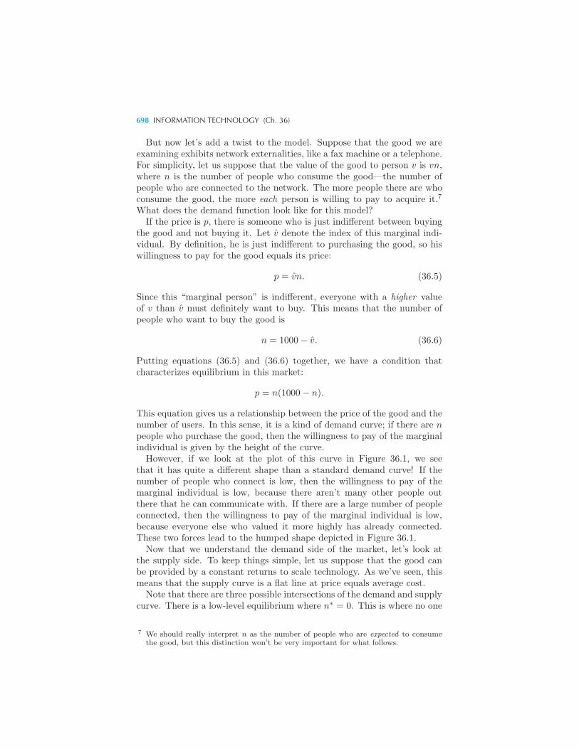
698 INFORMATION TECHNOLOGY (Ch. 36)
But now let’s add a twist to the model. Suppose that the good we areexamining exhibits network externalities, like a fax machine or a telephone.For simplicity, let us suppose that the value of the good to person v is vn,where n is the number of people who consume the good—the number ofpeople who are connected to the network. The more people there are whoconsume the good, the more each person is willing to pay to acquire it.7
What does the demand function look like for this model?If the price is p, there is someone who is just indifferent between buying
the good and not buying it. Let v denote the index of this marginal indi-vidual. By definition, he is just indifferent to purchasing the good, so hiswillingness to pay for the good equals its price:
p = vn. (36.5)
Since this “marginal person” is indifferent, everyone with a higher valueof v than v must definitely want to buy. This means that the number ofpeople who want to buy the good is
n = 1000− v. (36.6)
Putting equations (36.5) and (36.6) together, we have a condition thatcharacterizes equilibrium in this market:
p = n(1000− n).
This equation gives us a relationship between the price of the good and thenumber of users. In this sense, it is a kind of demand curve; if there are npeople who purchase the good, then the willingness to pay of the marginalindividual is given by the height of the curve.However, if we look at the plot of this curve in Figure 36.1, we see
that it has quite a different shape than a standard demand curve! If thenumber of people who connect is low, then the willingness to pay of themarginal individual is low, because there aren’t many other people outthere that he can communicate with. If there are a large number of peopleconnected, then the willingness to pay of the marginal individual is low,because everyone else who valued it more highly has already connected.These two forces lead to the humped shape depicted in Figure 36.1.Now that we understand the demand side of the market, let’s look at
the supply side. To keep things simple, let us suppose that the good canbe provided by a constant returns to scale technology. As we’ve seen, thismeans that the supply curve is a flat line at price equals average cost.Note that there are three possible intersections of the demand and supply
curve. There is a low-level equilibrium where n∗ = 0. This is where no one
7 We should really interpret n as the number of people who are expected to consumethe good, but this distinction won’t be very important for what follows.
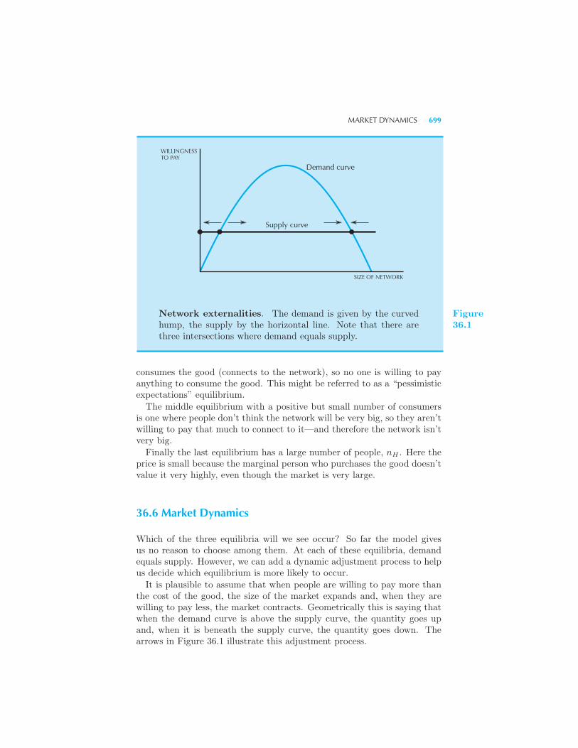
MARKET DYNAMICS 699
Supply curve
WILLINGNESSTO PAY
SIZE OF NETWORK
Demand curve
Network externalities. The demand is given by the curvedhump, the supply by the horizontal line. Note that there arethree intersections where demand equals supply.
Figure36.1
consumes the good (connects to the network), so no one is willing to payanything to consume the good. This might be referred to as a “pessimisticexpectations” equilibrium.
The middle equilibrium with a positive but small number of consumersis one where people don’t think the network will be very big, so they aren’twilling to pay that much to connect to it—and therefore the network isn’tvery big.
Finally the last equilibrium has a large number of people, nH . Here theprice is small because the marginal person who purchases the good doesn’tvalue it very highly, even though the market is very large.
36.6 Market Dynamics
Which of the three equilibria will we see occur? So far the model givesus no reason to choose among them. At each of these equilibria, demandequals supply. However, we can add a dynamic adjustment process to helpus decide which equilibrium is more likely to occur.
It is plausible to assume that when people are willing to pay more thanthe cost of the good, the size of the market expands and, when they arewilling to pay less, the market contracts. Geometrically this is saying thatwhen the demand curve is above the supply curve, the quantity goes upand, when it is beneath the supply curve, the quantity goes down. Thearrows in Figure 36.1 illustrate this adjustment process.
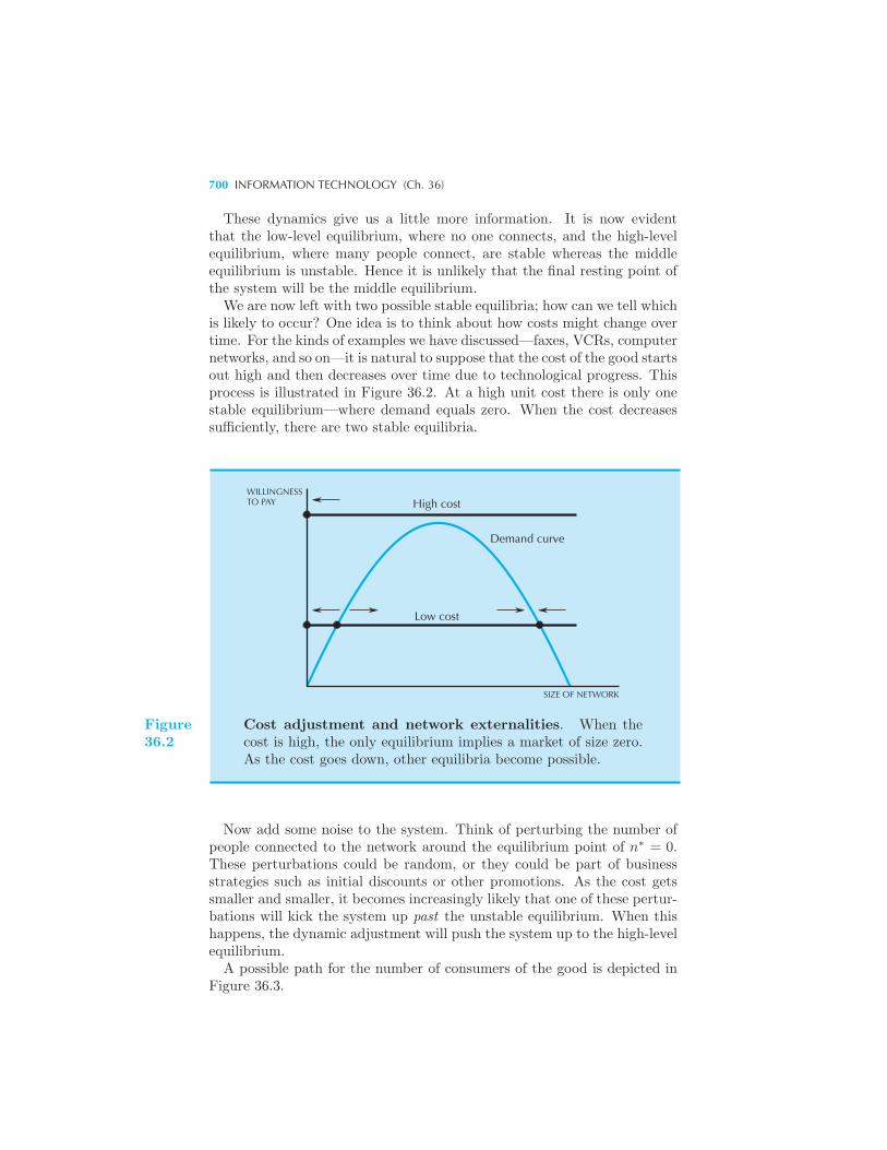
700 INFORMATION TECHNOLOGY (Ch. 36)
These dynamics give us a little more information. It is now evidentthat the low-level equilibrium, where no one connects, and the high-levelequilibrium, where many people connect, are stable whereas the middleequilibrium is unstable. Hence it is unlikely that the final resting point ofthe system will be the middle equilibrium.We are now left with two possible stable equilibria; how can we tell which
is likely to occur? One idea is to think about how costs might change overtime. For the kinds of examples we have discussed—faxes, VCRs, computernetworks, and so on—it is natural to suppose that the cost of the good startsout high and then decreases over time due to technological progress. Thisprocess is illustrated in Figure 36.2. At a high unit cost there is only onestable equilibrium—where demand equals zero. When the cost decreasessufficiently, there are two stable equilibria.
Low cost
WILLINGNESSTO PAY
SIZE OF NETWORK
Demand curve
High cost
Figure36.2
Cost adjustment and network externalities. When thecost is high, the only equilibrium implies a market of size zero.As the cost goes down, other equilibria become possible.
Now add some noise to the system. Think of perturbing the number ofpeople connected to the network around the equilibrium point of n∗ = 0.These perturbations could be random, or they could be part of businessstrategies such as initial discounts or other promotions. As the cost getssmaller and smaller, it becomes increasingly likely that one of these pertur-bations will kick the system up past the unstable equilibrium. When thishappens, the dynamic adjustment will push the system up to the high-levelequilibrium.A possible path for the number of consumers of the good is depicted in
Figure 36.3.
MARKET DYNAMICS 701
It starts out at essentially zero, with a few small perturbations over time.The cost decreases, and at some point we reach a critical mass that kicksus up past the low-level equilibrium and the system then zooms up to thehigh-level equilibrium.
Criticalmass
SIZE OFNETWORK
TIME
Possible adjustment to equilibrium. The number of usersconnected to the network is initially small, and increases onlygradually as costs fall. When a critical mass is reached, thenetwork growth takes off dramatically.
Figure36.3
A real-life example of this kind of adjustment is the market for fax ma-chines. Figure 36.4 illustrates the price and number of fax machines shippedover a period of 12 years.8
EXAMPLE: Network Externalities in Computer Software
Network externalities arise naturally in the provision of computer software.It is very convenient to be able to exchange data files and tips with other
8 This diagram is taken from “Critical Mass and Network Size with Applications tothe US Fax Market,” by Nicholas Economides and Charles Himmelberg (DiscussionPaper no. EC-95-11, Stern School of Business, N.Y.U., 1995). See also MichaelL. Katz and Carl Shapiro, “Systems Competition and Network Effects,” Journal ofEconomic Perspectives, 8 (1994), 93–116, for a nice overview of network externalitiesand their implications.
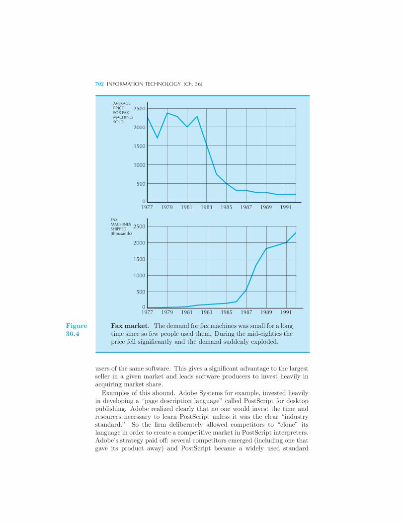
702 INFORMATION TECHNOLOGY (Ch. 36)
2500
2000
1500
1000
500
0
AVERAGE PRICEFOR FAXMACHINESSOLD
1977 1979 1981 1983 1985 1987 1989 1991
2500
2000
1500
1000
500
0
FAX MACHINESSHIPPED(thousands)
1977 1979 1981 1983 1985 1987 1989 1991
Figure36.4
Fax market. The demand for fax machines was small for a longtime since so few people used them. During the mid-eighties theprice fell significantly and the demand suddenly exploded.
users of the same software. This gives a significant advantage to the largestseller in a given market and leads software producers to invest heavily inacquiring market share.
Examples of this abound. Adobe Systems for example, invested heavilyin developing a “page description language” called PostScript for desktoppublishing. Adobe realized clearly that no one would invest the time andresources necessary to learn PostScript unless it was the clear “industrystandard.” So the firm deliberately allowed competitors to “clone” itslanguage in order to create a competitive market in PostScript interpreters.Adobe’s strategy paid off: several competitors emerged (including one thatgave its product away) and PostScript became a widely used standard
IMPLICATIONS OF NETWORK EXTERNALITIES 703
for desktop publishing. Adobe kept a few things proprietary—for instance,techniques for displaying fonts at low resolution—and managed to dominatethe high end of the market. Ironically, Adobe’s market success was due toits ability to encourage entry by its competitors!In recent years, many software producers have followed this model. Adobe
itself gives away several software products, such as the Adobe Acrobatreader. One of the hot new stock issues of 1995, Netscape Communica-tions Corporation, acquired the lion’s share of the Web browser market bygiving away its main product, making it a prime example of a companythat “lost money on every sale, but made up for it in volume.”
36.7 Implications of Network Externalities
The model described above, simple though it is, still yields a number ofinsights. For example, the critical mass issue is very important: if one user’sdemand depends on how many other users there are, it is very importantto try to stimulate growth early in the life cycle of a product. Nowadays itis quite common to see producers offering very cheap access to a piece ofsoftware or a communications service in order to “create a market” wherenone existed before.Of course, the critical question is how big does the market have to be
before it can take off on its own? Theory can provide little guidance here;everything depends on the nature of the good and the costs and benefitsthe users face in adopting it.Another important implication of network externalities is the role played
by governmental policy. The Internet is a prime example. The Internetwas originally used only by a few small research labs to exchange datafiles. In the mid-eighties the National Science Foundation used the Inter-net technology to connect several large universities to 12 supercomputersdeployed at various locations. The original vision was that researchersat the universities would send data back and forth to the supercomput-ers. But a fundamental property of communications networks is that ifyou are all connected to the same thing, you are all connected to eachother. This allowed researchers to send email to each other that hadnothing to do with the supercomputers. Once a critical mass of usershad been connected to the Internet, its value to new users increased dra-matically. Most of these new users had no interest in the supercomputercenters, even though this was the original motivation for providing thenetwork.
EXAMPLE: The Yellow Pages
The familiar local yellow pages phone directories are a $14 billion business.
704 INFORMATION TECHNOLOGY (Ch. 36)
Ten years ago, it was dominated by telephone companies, who had about95 percent of the market. Nowadays, they have only 85 percent.The difference is due to competition. Several small upstarts entered
the market in recent years, taking business away from the local phonecompanies. This is no easy task, as the local business directories exhibita classic form of network effects: it used to be that consumers all usedthe yellow page directory provided by their local phone companies, so localmerchants were forced to advertise in them.One upstart, Yellow Book, managed to overcome the network effects
by using clever business strategies, such as dramatically undercutting thephone companies’ ad rates and distributing its directory just before the lo-cal phone company’s directory came out. The incumbent providers, think-ing that their market was secure, dismissed the threat of aggressive new-comers until it was nearly too late. In the last few years, competitionhas heated up in this industry. This example goes to show that even in-dustries with strong network effects aren’t immune to competitive forces,particularly when the incumbents become overconfident.
EXAMPLE: Radio Ads
The “killer app” for radio in 1910 was ship-to-shore communication. Un-fortunately, radio conversations were not private since they were broadcastto anyone who tuned into the right frequency. At some point David Sarnoffrecognized that this bug might be a feature and offered a “radio music box”that sent music over the airwaves. His colleagues were skeptical, saying,“The wireless music box has no imaginable commercial value. Who wouldpay for a message sent to nobody in particular?”They had a point. Even though people found broadcast radio attractive,
the industry did not have a business model. How would they make money?The magazine Wireless World held a contest in which it proposed 5
business models for broadcast radio and people voted for their favorite.The business models were:
• support from general taxation;
• donations from the public;
• radio hardware makers subsidized the production of radio content;
• advertising-supported radio;
• vacuum tube tax used to support content production.
The winner was the last model: a tax on vacuum tubes. Some of theother models are still used today. BBC Radio and TV is supported by a tax
TWO-SIDED MARKETS 705
on TVs, and National Public Radio in the United States is supported bydonations from the public at large. However, in most countries advertisinghas become the most popular business model.In 1922, 30 radio stations were in operation in the United States, and
a hundred thousand radios were sold. By the next year there were 556stations with half-a-million receivers being sold. Radio was on its way.
36.8 Two-sided Markets
A two-sided market is a special kind of network effect. Think about thecase of a new technology, like Blu-ray DVDs. I don’t really care what sortof DVD player other people have, so there is no direct network effect. Butthere is a kind of indirect network effect: the more Blu-ray players that aresold, the more disks that will become available, and the more disks thereare available, the more attractive it will be to buy a Blu-ray player.One can think of many other examples. Consider a new credit card: the
more merchants accept the credit card, the more attractive the credit cardwill be to consumers. But the more consumers who adopt the card, themore attractive it will be to merchants.Or think about Adobe’s PDF platform. The more users who have the
PDF-viewing software (Acrobat Reader) the more graphics designers willwant to distribute content in this format, and the more demand there willbe for the Acrobat Distiller, the software used to create PDF files.This last example illustrates an important point: it may pay Adobe to
give away one product (Reader) in order to encourage demand for anotherproduct (Distiller). This is as old as “giving away the razor to sell theblades,” but since the combination of digital goods and the Internet hasmade distribution so cheap, the strategy has become very common.Apple, for example, sells the popular iPod music player. They also dis-
tribute music for the iPod on their iTunes store. According to industryreports, Apple makes very little money on the music—most of the profitsgo to the music studios. However, from Apple’s point of view it makessense to give away the blades (songs) to sell the razors (iPods).
A Model of Two-sided Markets
Let us generalize the model used in section 34.5 to apply to two-sidedmarkets.Suppose now that there are two goods. The reservation price for good
1 is v1 and it takes on values v1 = 1, . . . , 1000. Similarly the reservationprice for good 2 takes on values v2 = 1, . . . , 1000.
The total value for good 1 depends on how many people adopt good2, and the total value for good 2 depends on how many people adopt
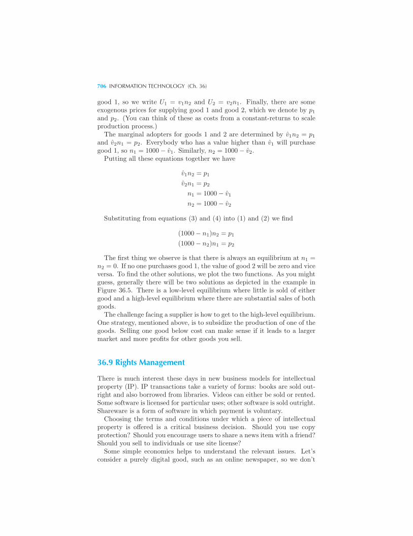
706 INFORMATION TECHNOLOGY (Ch. 36)
good 1, so we write U1 = v1n2 and U2 = v2n1. Finally, there are someexogenous prices for supplying good 1 and good 2, which we denote by p1and p2. (You can think of these as costs from a constant-returns to scaleproduction process.)The marginal adopters for goods 1 and 2 are determined by v1n2 = p1
and v2n1 = p2. Everybody who has a value higher than v1 will purchasegood 1, so n1 = 1000− v1. Similarly, n2 = 1000− v2.
Putting all these equations together we have
v1n2 = p1
v2n1 = p2
n1 = 1000− v1
n2 = 1000− v2
Substituting from equations (3) and (4) into (1) and (2) we find
(1000− n1)n2 = p1
(1000− n2)n1 = p2
The first thing we observe is that there is always an equilibrium at n1 =n2 = 0. If no one purchases good 1, the value of good 2 will be zero and viceversa. To find the other solutions, we plot the two functions. As you mightguess, generally there will be two solutions as depicted in the example inFigure 36.5. There is a low-level equilibrium where little is sold of eithergood and a high-level equilibrium where there are substantial sales of bothgoods.The challenge facing a supplier is how to get to the high-level equilibrium.
One strategy, mentioned above, is to subsidize the production of one of thegoods. Selling one good below cost can make sense if it leads to a largermarket and more profits for other goods you sell.
36.9 Rights Management
There is much interest these days in new business models for intellectualproperty (IP). IP transactions take a variety of forms: books are sold out-right and also borrowed from libraries. Videos can either be sold or rented.Some software is licensed for particular uses; other software is sold outright.Shareware is a form of software in which payment is voluntary.Choosing the terms and conditions under which a piece of intellectual
property is offered is a critical business decision. Should you use copyprotection? Should you encourage users to share a news item with a friend?Should you sell to individuals or use site license?Some simple economics helps to understand the relevant issues. Let’s
consider a purely digital good, such as an online newspaper, so we don’t
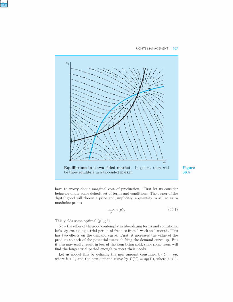
RIGHTS MANAGEMENT 707
n2
n1
Equilibrium in a two-sided market. In general there willbe three equilibria in a two-sided market.
Figure36.5
have to worry about marginal cost of production. First let us considerbehavior under some default set of terms and conditions. The owner of thedigital good will choose a price and, implicitly, a quantity to sell so as tomaximize profit:
maxy
p(y)y (36.7)
This yields some optimal (p∗, y∗).
Now the seller of the good contemplates liberalizing terms and conditions:let’s say extending a trial period of free use from 1 week to 1 month. Thishas two effects on the demand curve. First, it increases the value of theproduct to each of the potential users, shifting the demand curve up. Butit also may easily result in less of the item being sold, since some users willfind the longer trial period enough to meet their needs.
Let us model this by defining the new amount consumed by Y = by,where b > 1, and the new demand curve by P (Y ) = ap(Y ), where a > 1.
708 INFORMATION TECHNOLOGY (Ch. 36)
The new profit-maximization problem now becomes
maxY
P (Y )y.
Note that we multiply price times the amount sold, y, not the amountconsumed, Y .Applying the definitions Y = by and P (Y ) = ap(Y ), we can write this
as
maxY
ap(Y )Y
b= max
Y
a
bp(Y )Y.
This maximization problem looks like problem (36.7) except for the con-stant a/b in front of the max. This will not affect the optimal choice, sowe can conclude that Y ∗ = y∗.This simple analysis allows us to make several conclusions:
• The amount of the good consumed, Y ∗, is independent of the terms andconditions.
• The amount of the good produced is y∗/b which is less than y∗.
• The profits could go up or down depending on whether a/b is greater orless than 1. Profits go up if the increase in value to the consumers whobuy the product compensates for the reduced number of buyers.
EXAMPLE: Video Rental
Video stores can choose the terms and conditions under which they rentvideos. The longer you can keep the video, the more valuable it is to you,since you have a longer period of time during which you can watch it. Butthe longer you keep the video, the less profit the store makes from it, sinceit is unable to rent it to someone else. The optimal choice for the rentalperiod involves trading off these two effects.In practice, this has tended to lead to a form of product differentiation.
New releases are rented for short periods, since the the profits from otherrenters being excluded are very substantial. Older videos are rented forlonger periods, since there is less cost to the store from the video beingunavailable.
36.10 Sharing Intellectual Property
Intellectual property is often shared. Libraries, for example, facilitate thesharing of books. Video stores help people to “share” videos—and chargea price for doing so. Interlibrary loan helps libraries share books among
SHARING INTELLECTUAL PROPERTY 709
themselves. Even textbooks—such as the one you are holding—are sharedamong students from one term to the next via the resale market.
There is considerable debate in the publishing and library communitiesabout the proper role of sharing. Librarians have established an informal“rule of five” for interlibrary loan: an item may be loaned out up to fivetimes before additional royalty payments should be made to the publisher.Publishers and authors have traditionally been unenthusiastic about theresale market for books.
The advent of digital information has made this situation even moreacute. Digital information can be perfectly reproduced, and “sharing” canbe taken to new extremes. Recently, a well-known country music singerengaged in a vociferous public relations campaign against stores sellingused CDs. The problem was that CDs do not deteriorate with replay andit is possible to buy a CD, tape it, and then sell the CD to the used-CDstore.
Let us try to construct a model of this sort of sharing phenomenon. Webegin with the baseline case in which there is no sharing. In this case avideo maker chooses to produce y copies of a video to maximize profit:
maxy
p(y)y − cy − F. (36.8)
As usual, p(y) is the inverse demand function, c is the (constant) marginalcost, and F is the fixed cost. Let the profit maximizing output be denotedby yn, where the n stands for “no sharing.”
Now suppose that a video rental market is allowed. In this case the num-ber of videos viewed will be distinct from the number of copies produced.If y is the number of videos produced and each video is shared among kviewers, then the number of viewings will be x = ky. (For simplicity weare assuming that all copies of the video are rented in this case.)
We need to specify how the consumers sort themselves into the “clubs”that share the videos. The simplest assumption is that the consumers withhigh values associate with each other, and the consumers with low-valuesassociate with each other. That is, one club consists of consumers with thek highest values, another club consists of the consumers with the next khighest values, and so on. (Other assumptions could be used, but this onegives a very simple analysis.)
If y copies of the video are produced, x = ky copies will be viewed, so thewillingness to pay of the marginal individual will be p(x) = p(ky). However,it is clearly the case that there is some inconvenience cost to renting a videorather than owning it yourself. Let us denote this “transactions cost” by t,so that the willingness to pay of the marginal individual becomes p(x)− t.
Recall that we have assumed that all copies of the video are sharedamong k users. Therefore the willingness to pay of a video store will justbe k times the willingness to pay of the marginal individual. That is, if y
710 INFORMATION TECHNOLOGY (Ch. 36)
copies are produced, the willingness to pay of the video store will be
P (y) = k[p(ky)− t]. (36.9)
Equation (36.9) contains the two key effects that arise from sharing: thewillingness to pay goes down since more videos are viewed than are pro-duced; but the willingness to pay also goes up since the cost of a singlevideo is shared among several individuals.The profit maximization problem of the producer now becomes
maxy
P (y)y − cy − F,
which can be written as
maxy
k[p(ky)− t]y − cy − F,
ormax
yp(ky)ky −
( c
k+ t
)ky − F.
Recalling that the number of viewings, x, is related to the number pro-duced, y, via x = ky, we can also write the maximization problem as
maxx
p(x)x−( c
k+ t
)x− F.
Note that this problem is identical to problem (36.8), with the exceptionthat the marginal cost is now (c/k + t) rather than c.The close relationship between the two problems is very useful since it
allows us to make the following observation: profits will be larger whenrental is possible than when it is not if and only if
c
k+ t < c.
Rearranging this condition, we have(
k
k + 1
)t < c.
For large k, the fraction on the left is about 1. Hence the critical issueis the relationship between the marginal cost of production, c, and thetransactions cost of renting, t.If the cost of production is large and the cost of renting is small, then
the most profitable thing for a producer to do is to produce a few copies,sell them at a high price, and let the consumers rent. On the other hand,if the transactions cost of renting is larger than the cost of production, it ismore profitable for a producer to have renting prohibited: since renting isso inconvenient for the consumers, video stores aren’t willing to pay muchmore for the “shared” videos, and so the producer is better off selling.
SUMMARY 711
EXAMPLE: Online Two-sided Markets
There are several examples of two-sided markets on the Internet. For ex-ample, eBay serves as a meeting place for those who wish to buy and sellcollectibles. If you are selling rare coins, for example, you want to offerthem on a market where there are many potential buyers. Similarly, if youare a buyer, you want to go to a market where there are several competingsellers. This two-sided network effect tends to lead to a single meetingplace. In the last several years, eBay has expanded beyond collectibles andnow sells a variety of mechandise.Another set of interesting examples are social networking sites, such as
Facebook, MySpace, LinkedIn, and others. Participants want to registeron sites where their friends have registered. This again leads to a networkeffect—the largest network attracts the most new participants.Facebook has seen particularly rapid growth. It was launched in Febru-
ary of 2004 and by December of that year had 1 million active users. InSeptember of 2009, Facebook had over 300 million active users worldwide,according to statistics from its website.
Summary
1. Because information technology works together in systems, it is costlyto consumers to switch any one component.
2. If two monopoly providers of complementary products coordinate theirprice setting, then they will both set their prices lower than they wouldthan if they set them independently.
3. This will increase profit for the two monopolists and make consumersbetter off.
4. There are many ways to achieve this coordination, including merger,negotiation, revenue sharing, and commoditization.
5. In a lock-in equilibrium the discount offered first period is paid for byincreased prices in future periods.
6. Network externalities arise when one person’s willingness to pay for agood depends on the number of other users of that good.
7. Models with network externalities typically exhibit multiple equilibria.The ultimate outcome often depends on the history of the industry.
8. Rights management involves a tradeoff between increased value andprices versus reduced sales.

712 INFORMATION TECHNOLOGY (Ch. 36)
9. Information goods like books and videos are often rented or shared aswell as purchased. Rental or purchase can be more profitable dependingon how transactions costs compare with production costs.
REVIEW QUESTIONS
1. If the cost to a customer from switching long-distance carriers is on theorder of $50, how much should a long-distance carrier be willing to pay toacquire a new customer?
2. Describe how the demand for a word processing package might exhibitnetwork externalities.
3. Suppose that the marginal cost of producing an extra video is zero andthe transactions cost of renting a video is zero. Does a producer make moremoney by selling the video or by renting it?
CHAPTER 37
PUBLIC GOODS
In Chapter 35 we argued that for certain kinds of externalities, it was notdifficult to eliminate the inefficiencies. In the case of a consumption exter-nality between two people, for example, all one had to do was to ensure thatinitial property rights were clearly specified. People could then trade theright to generate the externality in the normal way. In the case of produc-tion externalities, the market itself provided profit signals to sort out theproperty rights in the most efficient way. In the case of common property,assigning property rights to someone would eliminate the inefficiency.Unfortunately, not all externalities can be handled in that manner. As
soon as there are more than two economic agents involved things becomemuch more difficult. Suppose, for example, that instead of the two room-mates examined in the last chapter, we had three roommates—one smokerand two nonsmokers. Then the amount of smoke would be a negativeexternality for both of the nonsmokers.Let’s suppose that property rights are well defined—say the nonsmokers
have the right to demand clean air. Just as before, although they have theright to clean air, they also have the right to trade some of that clean airaway in return for appropriate compensation. But now there is a prob-lem involved—the nonsmokers have to agree among themselves how muchsmoke should be allowed and what the compensation should be.

714 PUBLIC GOODS (Ch. 37)
Perhaps one of the nonsmokers is much more sensitive than the other, orone of them is much richer than the other. They may have very differentpreferences and resources, and yet they both have to reach some kind ofagreement to allow for an efficient allocation of smoke.Instead of roommates, we can think of inhabitants of a whole country.
How much pollution should be allowed in the country? If you think thatreaching an agreement is difficult with only three roommates, imagine whatit is like with millions of people!The smoke externality with three people is an example of a public
good—a good that must be provided in the same amount to all the af-fected consumers. In this case the amount of smoke generated will be thesame for all consumers—each person may value it differently, but they allhave to face the same amount.Many public goods are provided by the government. For example, streets
and sidewalks are provided by local municipalities. There are a certainnumber and quality of streets in a town, and everyone has that numberavailable to use. National defense is another good example; there is onelevel of national defense provided for all the inhabitants of a country. Eachcitizen may value it differently—some may want more, some may wantless—but they are all provided with the same amount.Public goods are an example of a particular kind of consumption exter-
nality: everyone must consume the same amount of the good. They are aparticularly troublesome kind of externality, for the decentralized marketsolutions that economists are fond of don’t work very well in allocatingpublic goods. People can’t purchase different amounts of public defense;somehow they have to decide on a common amount.The first issue to examine is what the ideal amount of the public good
should be. Then we’ll discuss some ways that might be used to make socialdecisions about public goods.
37.1 When to Provide a Public Good?
Let us start with a simple example. Suppose that there are two roommates,1 and 2. They are trying to decide whether or not to purchase a TV. Giventhe size of their apartment, the TV will necessarily go in the living room,and both roommates will be able to watch it. Thus it will be a publicgood, rather than a private good. The question is, is it worth it for themto acquire the TV?Let’s use w1 and w2 to denote each person’s initial wealth, g1 and g2 to
denote each person’s contribution to the TV, and x1 and x2 to denote eachperson’s money left over to spend on private consumption. The budgetconstraints are given by
x1 + g1 = w1
x2 + g2 = w2.
WHEN TO PROVIDE A PUBLIC GOOD? 715
We also suppose that the TV costs c dollars, so that in order to purchaseit, the sum of the two contributions must be at least c:
g1 + g2 ≥ c.
This equation summarizes the technology available to provide the publicgood: the roommates can acquire one TV if together they pay the cost c.The utility function of person 1 will depend on his or her private con-
sumption, x1, and the availability of the TV—the public good. We’ll writeperson 1’s utility function as u1(x1, G), where G will either be 0, indicatingno TV, or 1, indicating that a TV is present. Person 2 will have utilityfunction u2(x2, G). Each person’s private consumption has a subscript toindicate that the good is consumed by person 1 or person 2, but the publicgood has no subscript. It is “consumed” by both people. Of course, it isn’treally consumed in the sense of being “used up”; rather, it is the servicesof the TV that are consumed by the two roommates.The roommates may value the services of the TV quite differently. We
can measure the value that each person places on the TV by asking howmuch each person would be willing to pay to have the TV available. To dothis, we’ll use the concept of the reservation price, introduced in Chapter15.The reservation price of person 1 is the maximum amount that person 1
would be willing to pay to have the TV present. That is, it is that price,r1, such that person 1 is just indifferent between paying r1 and havingthe TV available, and not having the TV at all. If person 1 pays thereservation price and gets the TV, he will have w1−r1 available for privateconsumption. If he doesn’t get the TV, he will have w1 available for privateconsumption. If he is to be just indifferent between these two alternatives,we must have
u1(w1 − r1, 1) = u1(w1, 0).
This equation defines the reservation price for person 1—the maximumamount that he would be willing to pay to have the TV present. A similarequation defines the reservation price for person 2. Note that in generalthe reservation price of each person will depend on that person’s wealth:the maximum amount that an individual will be willing to pay will dependto some degree on how much that individual is able to pay.
Recall that an allocation is Pareto efficient if there is no way to makeboth people better off. An allocation is Pareto inefficient if there is someway to make both people better off; in this case, we say that a Paretoimprovement is possible. In the TV problem there are only two sorts ofallocations that are of interest. One is an allocation where the TV is notprovided. This allocation takes the simple form (w1, w2, 0); that is, eachperson spends his wealth only on his private consumption.The other kind of allocation is the one where the public good is provided.
This will be an allocation of the form (x1, x2, 1), where
x1 = w1 − g1
716 PUBLIC GOODS (Ch. 37)
x2 = w2 − g2.
These two equations come from rewriting the budget constraints. They saythat each individual’s private consumption is determined by the wealth thathe has left over after making his contribution to the public good.Under what conditions should the TV be provided? That is, when is
there a payment scheme (g1, g2) such that both people will be better offhaving the TV and paying their share than not having the TV? In thelanguage of economics, when will it be a Pareto improvement to providethe TV?It will be a Pareto improvement to provide the allocation (x1, x2, 1) if
both people would be better off having the TV provided than not havingit provided. This means
u1(w1, 0) < u1(x1, 1)
u2(w2, 0) < u2(x2, 1).
Now use the definition of the reservation prices r1 and r2 and the budgetconstraint to write
u1(w1 − r1, 1) = u1(w1, 0) < u1(x1, 1) = u1(w1 − g1, 1)
u2(w2 − r2, 1) = u2(w2, 0) < u2(x2, 1) = u2(w2 − g2, 1).
Looking at the left- and the right-hand sides of these inequalities, andremembering that more private consumption must increase utility, we canconclude that
w1 − r1 < w1 − g1
w2 − r2 < w2 − g2,
which in turn impliesr1 > g1
r2 > g2.
This is a condition that must be satisfied if an allocation (w1, w2, 0)is Pareto inefficient: it must be that the contribution that each personis making to the TV is less than his willingness to pay for the TV. If aconsumer can acquire the good for less than the maximum that he wouldbe willing to pay, then the acquisition would be to his benefit. Thus thecondition that the reservation price exceeds the cost share simply says thata Pareto improvement will result when each roommate can acquire theservices of the TV for less than the maximum that he would be willing topay for it. This is clearly a necessary condition for purchase of the TV tobe a Pareto improvement.If each roommate’s willingness to pay exceeds his cost share, then the
sum of the willingnesses to pay must be greater than the cost of the TV:
r1 + r2 > g1 + g2 = c. (37.1)
WHEN TO PROVIDE A PUBLIC GOOD? 717
This condition is a sufficient condition for it to be a Pareto improvementto provide the TV. If the condition is satisfied, then there will be somepayment plan such that both people will be made better off by providingthe public good. If r1 + r2 ≥ c, then the total amount that the roommateswill be willing to pay is at least as large as the cost of purchase, so theycan easily find a payment plan (g1, g2) such that r1 ≥ g1, r2 ≥ g2, andg1 + g2 = c. This condition is so simple that you might wonder why wewent through all the detail in deriving it. Well, there are a few subtletiesinvolved.First, it is important to note that the condition describing when pro-
vision of the public good will be a Pareto improvement only depends oneach agent’s willingness to pay and on the total cost. If the sum of thereservation prices exceeds the cost of the TV, then there will always exist apayment scheme such that both people will be better off having the publicgood than not having it.Second, whether or not it is Pareto efficient to provide the public good
will, in general, depend on the initial distribution of wealth (w1, w2). Thisis true because, in general, the reservation prices r1 and r2 will depend onthe distribution of wealth. It perfectly possible that for some distributionsof wealth r1 + r2 > c, and for other distributions of wealth r1 + r2 < c.
To see how this can be, imagine a situation where one roommate reallyloves the TV and the other roommate is nearly indifferent about acquiringit. Then if the TV-loving roommate had all of the wealth, he would bewilling to pay more than the cost of the TV all by himself. Thus it would bea Pareto improvement to provide the TV. But if the indifferent roommatehad all of the wealth, then the TV lover wouldn’t have much money tocontribute toward the TV, and it would be Pareto efficient not to providethe TV.Thus, in general, whether or not the public good should be provided will
depend on the distribution of wealth. But in specific cases the provision ofthe public good may be independent of the distribution of wealth. For ex-ample, suppose that the preferences of the two roommates were quasilinear.This means that the utility functions take the form
u1(x1, G) = x1 + v1(G)
u2(x2, G) = x2 + v2(G),
where G will be 0 or 1, depending on whether or not the public good isavailable. For simplicity, suppose that v1(0) = v2(0) = 0. This says thatno TV provides zero utility from watching TV.1
In this case the definitions of the reservation prices become
u1(w1 − r1, 1) = w1 − r1 + v1(1) = u1(w1, 0) = w1
u2(w2 − r2, 1) = w2 − r2 + v2(1) = u2(w2, 0) = w2,
1 Perhaps watching TV should be assigned a negative utility.
718 PUBLIC GOODS (Ch. 37)
which implies that the reservation prices are given by
r1 = v1(1)
r2 = v2(1).
Thus the reservation prices are independent of the amount of wealth, andhence the optimal provision of the public good will be independent ofwealth, at least over some range of wealths.2
37.2 Private Provision of the Public Good
We have seen above that acquiring the TV will be Pareto efficient for thetwo roommates if the sum of their willingnesses to pay exceeds the cost ofproviding the public good. This answers the question about efficient allo-cation of the good, but it does not necessarily follow that they will actuallydecide to acquire the TV. Whether they actually decide to acquire the TVdepends on the particular method they adopt to make joint decisions.If the two roommates cooperate and truthfully reveal how much they
value the TV, then it should not be difficult for them to agree on whetheror not they should buy the TV. But under some circumstances, they maynot have incentives to tell the truth about their values.For example, suppose that each person valued the TV equally, and that
each person’s reservation price was greater than the cost, so that r1 > cand r2 > c. Then person 1 might think that if he said he had 0 value forthe TV, the other person would acquire it anyway. But person 2 couldreason the same way! One can imagine other situations where both peoplewould refuse to contribute in the hopes that the other person would go outand unilaterally purchase the TV.In this kind of situation, economists say that the people are attempting
to free ride on each other: each person hopes that the other person willpurchase the public good on his own. Since each person will have full useof the services of the TV if it is acquired, each person has an incentive totry to pay as little as possible toward the provision of the TV.
37.3 Free Riding
Free riding is similar, but not identical, to the prisoner’s dilemma that weexamined in Chapter 29. To see this, let us construct a numerical exampleof the TV problem described above. Suppose that each person has a wealthof $500, that each person values the TV at $100, and that the cost of the
2 Even this will only be true for some ranges of wealth, since we must always requirethat r1 ≤ w1 and r2 ≤ w2—i.e., the willingness to pay is less than the ability to pay.
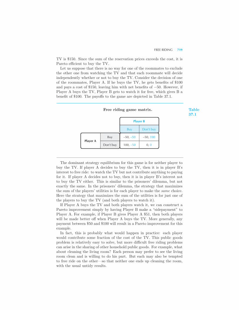
FREE RIDING 719
TV is $150. Since the sum of the reservation prices exceeds the cost, it isPareto efficient to buy the TV.Let us suppose that there is no way for one of the roommates to exclude
the other one from watching the TV and that each roommate will decideindependently whether or not to buy the TV. Consider the decision of oneof the roommates, Player A. If he buys the TV, he gets benefits of $100and pays a cost of $150, leaving him with net benefits of −50. However, ifPlayer A buys the TV, Player B gets to watch it for free, which gives B abenefit of $100. The payoffs to the game are depicted in Table 37.1.
Player B
Player ABuy
Don’t buy
–50, –50
100, –50
–50, 100
0, 0
Buy Don’t buy
Free riding game matrix. Table37.1
The dominant strategy equilibrium for this game is for neither player tobuy the TV. If player A decides to buy the TV, then it is in player B’sinterest to free ride: to watch the TV but not contribute anything to payingfor it. If player A decides not to buy, then it is in player B’s interest notto buy the TV either. This is similar to the prisoners’ dilemma, but notexactly the same. In the prisoners’ dilemma, the strategy that maximizesthe sum of the players’ utilities is for each player to make the same choice.Here the strategy that maximizes the sum of the utilities is for just one ofthe players to buy the TV (and both players to watch it).If Player A buys the TV and both players watch it, we can construct a
Pareto improvement simply by having Player B make a “sidepayment” toPlayer A. For example, if Player B gives Player A $51, then both playerswill be made better off when Player A buys the TV. More generally, anypayment between $50 and $100 will result in a Pareto improvement for thisexample.In fact, this is probably what would happen in practice: each player
would contribute some fraction of the cost of the TV. This public goodsproblem is relatively easy to solve, but more difficult free riding problemscan arise in the sharing of other household public goods. For example, whatabout cleaning the living room? Each person may prefer to see the livingroom clean and is willing to do his part. But each may also be temptedto free ride on the other—so that neither one ends up cleaning the room,with the usual untidy results.
720 PUBLIC GOODS (Ch. 37)
The situation becomes even worse if there are more than just two peopleinvolved—since there are more people on whom to free ride! Letting theother guy do it may be optimal from an individual point of view, but it isPareto inefficient from the viewpoint of society as a whole.
37.4 Different Levels of the Public Good
In the above example, we had an either/or decision: either provide the TVor not. But the same kind of phenomena occurs when there is a choice ofhow much of the public good to provide. Suppose, for example, that thetwo roommates have to decide how much money to spend on the TV. Themore money they decide to spend, the better the TV they can get.As before we’ll let x1 and x2 measure the private consumption of each
person and g1 and g2 be their contributions to the TV. Let G now measurethe “quality” of the TV they buy, and let the cost function for quality begiven by c(G). This means that if the two roommates want to purchase aTV of quality G, they have to spend c(G) dollars to do so.The constraint facing the roommates is that the total amount that they
spend on their public and private consumption has to add up to how muchmoney they have:
x1 + x2 + c(G) = w1 + w2.
A Pareto efficient allocation is one where consumer 1 is as well-off aspossible given consumer 2’s level of utility. If we fix the utility of consumer2 at u2, we can write this problem as
maxx1,x2,G
u1(x1, G)
such that u2(x2, G) = u2
x1 + x2 + c(G) = w1 + w2.
It turns out that the appropriate optimality condition for this problemis that the sum of the absolute values of the marginal rates of substitutionbetween the private good and the public good for the two consumers equalsthe marginal cost of providing an extra unit of the public good:
|MRS1|+ |MRS2| = MC(G)
or, spelling out the definitions of the marginal rates of substitution,
∣∣∣∣Δx1
ΔG
∣∣∣∣+∣∣∣∣Δx2
ΔG
∣∣∣∣ = MUG
MUx1
+MUG
MUx2
= MC(G).
In order to see why this must be the right efficiency condition, let usapply the usual trick and think about what would be the case if it were
DIFFERENT LEVELS OF THE PUBLIC GOOD 721
violated. Suppose, for example, that the sum of the marginal rates ofsubstitution were less than the marginal cost: say MC = 1, |MRS1| = 1/4,and |MRS2| = 1/2. We need to show that there is some way to make bothpeople better off.Given his marginal rate of substitution, we know that person 1 would be
willing to accept 1/4 more dollars of the private good for the loss of 1 dollarof the public good (since both goods cost $1 per unit). Similarly, person 2would accept 1/2 more dollars of the private good for a 1-dollar decreasein the public good. Suppose we reduce the amount of the public good andoffer to compensate both individuals. When we reduce the public good byone unit we save a dollar. After we pay each individual the amount herequires to allow this change (3/4 = 1/4 + 1/2), we find that we still have1/4 of a dollar left over. This remaining money could be shared betweenthe two individuals, thereby making them both better off.Similarly, if the sum of the marginal rates of substitution were greater
than 1, we could increase the amount of the public good to make themboth better off. If |MRS1| = 2/3 and |MRS2| = 1/2, say, this means thatperson 1 would give up 2/3 of a dollar of private consumption to get 1unit more of the public good and person 2 would give up 1/2 of a dollar ofprivate consumption to get 1 unit more of the public good. But if person 1gave up his 2/3 units, and person 2 gave up his 1/2 unit, we would havemore than enough to produce the extra unit of the public good, since themarginal cost of providing the public good is 1. Thus we could give theleft-over amount back to both people, thereby making them both better off.What does the condition for Pareto efficiency mean? One way to inter-
pret it is to think of the marginal rate of substitution as measuring themar-ginal willingness to pay for an extra unit of the public good. Then the effi-ciency condition just says that the sum of the marginal willingnesses to paymust equal the marginal cost of providing an extra unit of the public good.In the case of a discrete good that was either provided or not provided,
we said that the efficiency condition was that the sum of the willingnessesto pay should be at least as large as the cost. In the case we’re consideringhere, where the public good can be provided at different levels, the efficiencycondition is that the sum of the marginal willingnesses to pay should equalthe marginal cost at the optimal amount of the public good. For wheneverthe sum of the marginal willingnesses to pay for the public good exceedsthe marginal cost, it is appropriate to provide more of the public good.It is worthwhile comparing the efficiency condition for a public good
to the efficiency condition for a private good. For a private good, eachperson’s marginal rate of substitution must equal the marginal cost; for apublic good, the sum of the marginal rates of substitution must equal themarginal cost. In the case of a private good, each person can consume adifferent amount of the private good, but they all must value it the sameat the margin—otherwise they would want to trade. In the case of a publicgood, each person must consume the same amount of the public good, but
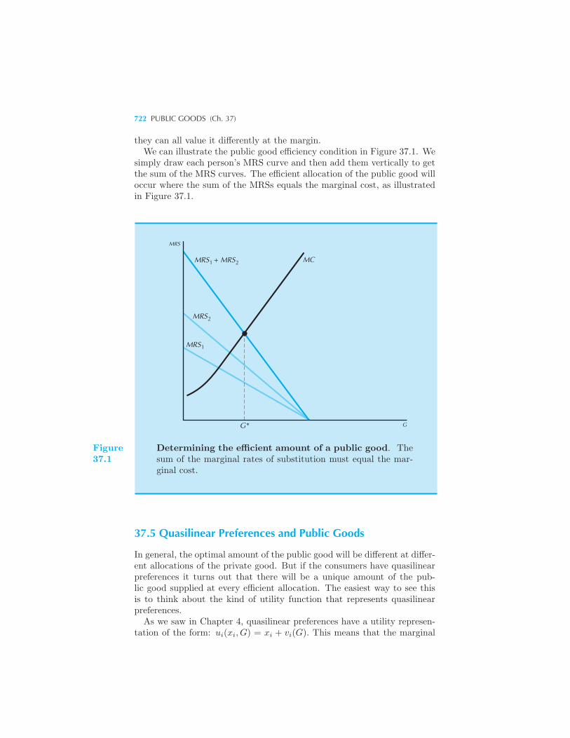
722 PUBLIC GOODS (Ch. 37)
they can all value it differently at the margin.We can illustrate the public good efficiency condition in Figure 37.1. We
simply draw each person’s MRS curve and then add them vertically to getthe sum of the MRS curves. The efficient allocation of the public good willoccur where the sum of the MRSs equals the marginal cost, as illustratedin Figure 37.1.
MRS
MCMRS + MRS
MRS
MRS
G* G
2
1
1 2
Figure37.1
Determining the efficient amount of a public good. Thesum of the marginal rates of substitution must equal the mar-ginal cost.
37.5 Quasilinear Preferences and Public Goods
In general, the optimal amount of the public good will be different at differ-ent allocations of the private good. But if the consumers have quasilinearpreferences it turns out that there will be a unique amount of the pub-lic good supplied at every efficient allocation. The easiest way to see thisis to think about the kind of utility function that represents quasilinearpreferences.As we saw in Chapter 4, quasilinear preferences have a utility represen-
tation of the form: ui(xi, G) = xi + vi(G). This means that the marginal
QUASILINEAR PREFERENCES AND PUBLIC GOODS 723
utility of the private good is always 1, and thus the marginal rate of substi-tution between the private and the public good—the ratio of the marginalutilities—will depend only on G. In particular:
|MRS1| =Δu1(x1, G)/ΔG
Δu1/Δx1=
Δv1(G)
ΔG
|MRS2| =Δu2(x2, G)/ΔG
Δu2/Δx2=
Δv2(G)
ΔG.
We already know that a Pareto efficient level of the public good mustsatisfy the condition
|MRS1|+ |MRS2| = MC(G).
Using the special form of the MRSs in the case of quasilinear utility, wecan write this condition as
Δv1(G)
ΔG+
Δv2(G)
ΔG= MC(G).
Note that this equation determines G without any reference to x1 or x2.Thus there is a unique efficient level of provision of the public good.Another way to see this is to think about the behavior of the indifference
curves. In the case of quasilinear preferences, all of the indifference curvesare just shifted versions of each other. This means, in particular, that theslope of the indifference curves—the marginal rate of substitution—doesn’tchange as we change the amount of the private good. Suppose that we findone efficient allocation of the public and private goods, where the sum of theabsolute value of the MRSs equals MC(G). Now if we take some amountof the private good away from one person and give it to another, the slopesof both indifference curves stay the same, so the sum of the absolute valueof the MRSs is still equal to MC(G) and we have another Pareto efficientallocation.In the case of quasilinear preferences, all Pareto efficient allocations are
found by just redistributing the private good. The amount of the publicgood stays fixed at the efficient level.
EXAMPLE: Pollution Revisited
Recall the model of the steel firm and the fishery described in Chapter 35.There we argued that the efficient provision of pollution was one whichinternalized the pollution costs borne by the steel firm and the fishery.Suppose now that there are two fisheries, and that the amount of pollutionproduced by the steel firm is a public good. (Or, perhaps more appropri-ately, is a public bad!)
724 PUBLIC GOODS (Ch. 37)
Then the efficient provision of pollution will involve maximizing the sumof the profits of all three firms—that is, minimizing the total social cost ofthe pollution. Formally, let cs(s, x) be the cost to the steel firm of producings units of steel and x units of pollution, and write c1f (f1, x) for the costs
for firm 1 to catch f1 fish when the pollution level is x, and c2f (f2, x) asthe analogous expression for firm 2. Then to compute the Pareto efficientamount of pollution, we maximize the sum of the three firms’ profits:
maxs,f1,f2,x
pss+ pff1 + pff2 − cs(s, x)− c1f (f1, x)− c2f (f2, x).
The interesting effect for our purposes is the effect on aggregate profitsof increasing pollution. Increasing pollution lowers the cost of producingsteel but raises the costs of producing fish for each of the fisheries. Theappropriate optimality condition from the profit-maximization problem is
Δcs(s, x)
Δx+
Δc1f (f1, x)
Δx+
Δc2f (f2, x)
Δx= 0,
which simply says that the sum of the marginal costs of pollution over thethree firms should equal zero. Just as in the case of a public consumptiongood, it is the sum of the marginal benefits or costs over the economicagents that is relevant for determining the Pareto efficient provision of apublic good.
37.6 The Free Rider Problem
Now that we know what the Pareto efficient allocations of public goodsare, we can turn our attention to asking how to get there. In the case ofprivate goods with no externalities we saw that the market mechanism willgenerate an efficient allocation. Will the market work in the case of publicgoods?We can think of each person as having some endowment of a private
good, wi. Each person can spend some fraction of this private good onhis own private consumption, or he or she can contribute some of it topurchase the public good. Let’s use x1 for 1’s private consumption, and letg1 denote the amount of the public good he buys, and similarly for person 2.Suppose for simplicity that c(G) ≡ G, which implies that the marginal costof providing a unit of the public good is constant at 1. The total amountof the public good provided will be G = g1 + g2. Since each person caresabout the total amount of the public good provided, the utility function ofperson i will have the form ui(xi, g1 + g2) = ui(xi, G).
In order for person 1 to decide how much he should contribute to thepublic good, he has to have some forecast of how much person 2 will con-tribute. The simplest thing to do here is to adopt the Nash equilibrium
THE FREE RIDER PROBLEM 725
model described in Chapter 29, and suppose that person 2 will make somecontribution g2. We assume that person 2 also makes a guess about per-son 1’s contribution, and we look for an equilibrium where each person ismaking an optimal contribution given the other person’s behavior.Thus person 1’s maximization problem takes the form
maxx1,g1
u1(x1, g1 + g2)
such that x1 + g1 = w1.
This is just like an ordinary consumer maximization problem. The op-timization condition is therefore the same: if both people purchase bothgoods the marginal rate of substitution between the public and the privategoods should be 1 for each consumer:
|MRS1| = 1
|MRS2| = 1.
However, we have to be careful here. It is true that if person 2 purchasesany amount of the public good at all, he will purchase it until the marginalrate of substitution equals one. But it can easily happen that person 2 de-cides that the amount already contributed by person 1 is sufficient and thatit would therefore be unnecessary for him to contribute anything towardthe public good at all.Formally, we are assuming that the individuals can only make positive
contributions to the public good—they can put money into the collectionplate, but they can’t take money out. Thus there is an extra constrainton each person’s contributions, namely, that g1 ≥ 0 and g2 ≥ 0. Eachperson can only decide whether or not he wants to increase the amountof the public good. But then it may well be that one person decides thatthe amount provided by the other is just fine and would prefer to make nocontribution at all.A case like this is depicted in Figure 37.2. Here we have illustrated
each person’s private consumption on the horizontal axis and his or herpublic consumption on the vertical axis. The “endowment” of each personconsists of his or her wealth, wi, along with the amount of the public goodcontribution of the other person—since this is how much of the public goodwill be available if the person in question decides not to contribute. Figure37.2A shows a case where person 1 is the only contributor to the publicgood, so that g1 = G. If person 1 contributes G units to the public good,then person 2’s endowment will consist of her private wealth, w2, and theamount of the public good G—since person 2 gets to consume the publicgood whether or not she contributes to it. Since person 2 cannot reduce theamount of the public good, but can only increase it, her budget constraintis the bold line in Figure 37.2B. Given the shape of 2’s indifference curve,
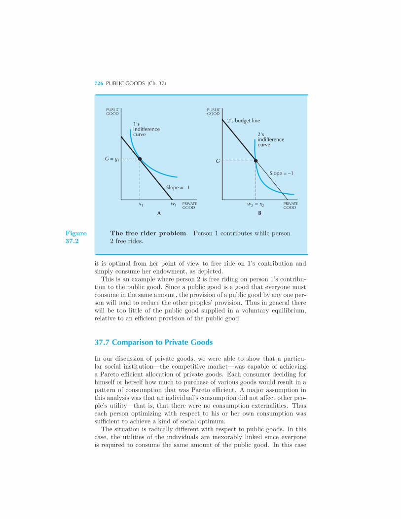
726 PUBLIC GOODS (Ch. 37)
PUBLICGOOD
PUBLICGOOD
1'sindifferencecurve 2's
indifferencecurve
G = g
Slope = –1
2's budget line
Slope = –1
G
x w w = x
A B
PRIVATEGOOD
PRIVATEGOOD1 1
1
2 2
Figure37.2
The free rider problem. Person 1 contributes while person2 free rides.
it is optimal from her point of view to free ride on 1’s contribution andsimply consume her endowment, as depicted.This is an example where person 2 is free riding on person 1’s contribu-
tion to the public good. Since a public good is a good that everyone mustconsume in the same amount, the provision of a public good by any one per-son will tend to reduce the other peoples’ provision. Thus in general therewill be too little of the public good supplied in a voluntary equilibrium,relative to an efficient provision of the public good.
37.7 Comparison to Private Goods
In our discussion of private goods, we were able to show that a particu-lar social institution—the competitive market—was capable of achievinga Pareto efficient allocation of private goods. Each consumer deciding forhimself or herself how much to purchase of various goods would result in apattern of consumption that was Pareto efficient. A major assumption inthis analysis was that an individual’s consumption did not affect other peo-ple’s utility—that is, that there were no consumption externalities. Thuseach person optimizing with respect to his or her own consumption wassufficient to achieve a kind of social optimum.The situation is radically different with respect to public goods. In this
case, the utilities of the individuals are inexorably linked since everyoneis required to consume the same amount of the public good. In this case
VOTING 727
the market provision of public goods would be very unlikely to result in aPareto efficient provision.Indeed, for the most part we use different social institutions to determine
the provision of public goods. Sometimes people use a command mech-anism, where one person or small group of people determines the amountof various public goods that will be provided by the populace. Other timespeople use a voting system where individuals vote on the provision ofpublic goods. One can well ask the same sorts of questions about voting,or other social mechanisms for decision making, that we asked about theprivate market: are they capable of achieving a Pareto efficient allocationof public goods? Can any Pareto efficient allocation of public goods beachieved by such mechanisms? A complete analysis of these questions isbeyond the scope of this book, but we will be able to shed a little light onhow some methods work below.
37.8 Voting
Private provision of a public good doesn’t work very well, but there areseveral other mechanisms for social choice. One of the most common mech-anisms in democratic countries is voting. Let’s examine how well it worksfor the provision of public goods.Voting isn’t very interesting in the case of two consumers, so we will sup-
pose that we have n consumers. Furthermore, so as not to worry about ties,we’ll suppose that n is an odd number. Let’s imagine that the consumersare voting about the size of some public good—say the magnitude of ex-penditures on public defense. Each consumer has a most-preferred level ofexpenditure, and his valuation of other levels of expenditure depends onhow close they are to his preferred level of expenditure.The first problem with voting as a way of determining social outcomes
has already been examined in Chapter 34. Suppose that we are consideringthree levels of expenditure, A, B, and C. It is perfectly possible that thereis a majority of the consumers who prefer A to B, a majority who prefer Bto C . . . and a majority who prefer C to A!Using the terminology of Chapter 34, the social preferences generated by
these consumers are not transitive. This means that the outcome of votingon the level of public good may not be well defined—there is always a levelof expenditure that beats every expenditure. If a society is allowed to votemany times on an issue, this means that it may “cycle” around variouschoices. Or if a society votes only once on an issue, the outcome dependson the order in which the choices are presented.If first you vote on A versus B and then on A versus C, C will be the
outcome. But if you vote on C versus A and then C versus B, B will bethe outcome. You can get any of the three outcomes by choosing how thealternatives are presented!
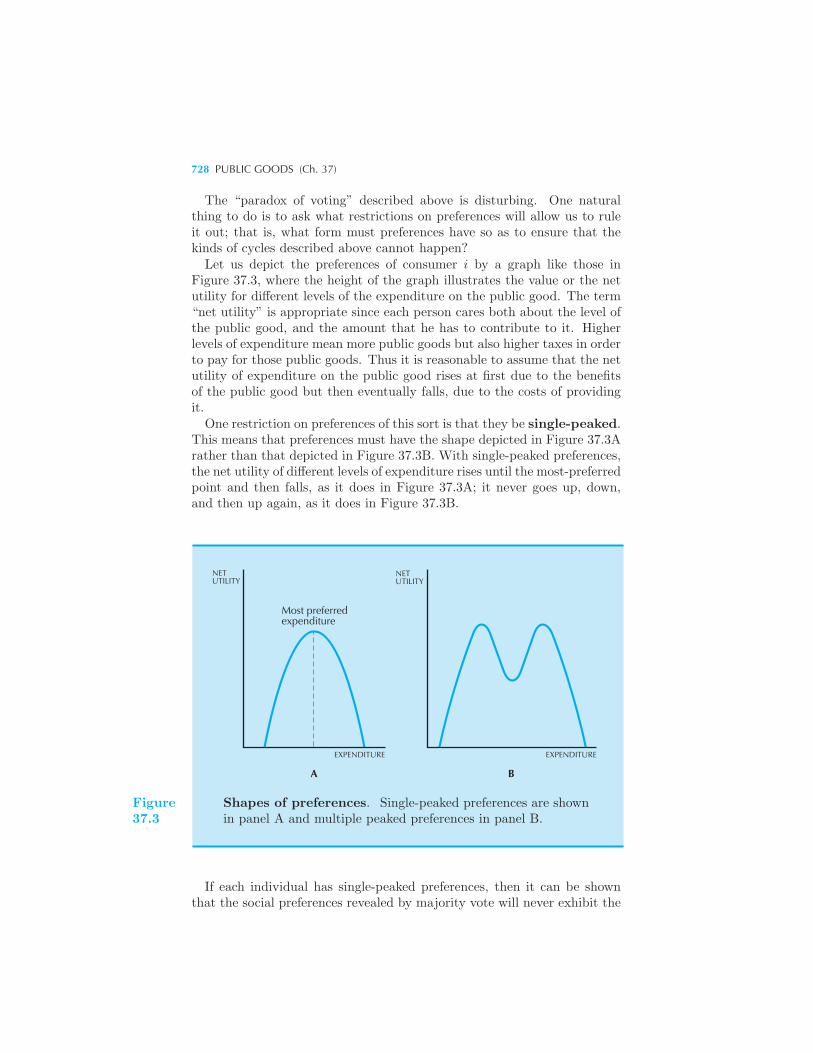
728 PUBLIC GOODS (Ch. 37)
The “paradox of voting” described above is disturbing. One naturalthing to do is to ask what restrictions on preferences will allow us to ruleit out; that is, what form must preferences have so as to ensure that thekinds of cycles described above cannot happen?Let us depict the preferences of consumer i by a graph like those in
Figure 37.3, where the height of the graph illustrates the value or the netutility for different levels of the expenditure on the public good. The term“net utility” is appropriate since each person cares both about the level ofthe public good, and the amount that he has to contribute to it. Higherlevels of expenditure mean more public goods but also higher taxes in orderto pay for those public goods. Thus it is reasonable to assume that the netutility of expenditure on the public good rises at first due to the benefitsof the public good but then eventually falls, due to the costs of providingit.One restriction on preferences of this sort is that they be single-peaked.
This means that preferences must have the shape depicted in Figure 37.3Arather than that depicted in Figure 37.3B. With single-peaked preferences,the net utility of different levels of expenditure rises until the most-preferredpoint and then falls, as it does in Figure 37.3A; it never goes up, down,and then up again, as it does in Figure 37.3B.
NETUTILITY
EXPENDITURE
NETUTILITY
EXPENDITURE
A B
Most preferredexpenditure
Figure37.3
Shapes of preferences. Single-peaked preferences are shownin panel A and multiple peaked preferences in panel B.
If each individual has single-peaked preferences, then it can be shownthat the social preferences revealed by majority vote will never exhibit the
VOTING 729
kind of intransitivity we described above. Accepting this result for the mo-ment, we can ask which level of expenditure will be chosen if everyone hassingle-peaked preferences. The answer turns out to be the median ex-penditure—that expenditure such that one-half of the population wantsto spend more, and one-half wants to spend less. This result is reasonablyintuitive: if more than one-half wanted more expenditure on the publicgood, they would vote for more, so the only possible equilibrium votingoutcome is when the votes for increasing and decreasing expenditure onthe public good are just balanced.Will this be an efficient level of the public good? In general, the answer is
no. The median outcome just means that half the population wants moreand half wants less; it doesn’t say anything about how much more theywant of the public good. Since efficiency takes this kind of informationinto account, voting will not in general lead to an efficient outcome.Furthermore, even if peoples’ true preferences are single-peaked, so that
voting may lead to a reasonable outcome, individuals may choose to mis-represent their true preferences when they vote. Thus people will have anincentive to vote differently than their true preferences would indicate inorder to manipulate the final outcome.
EXAMPLE: Agenda Manipulation
We have seen that the outcome of a sequence of votes may depend on theorder in which the votes are taken. Experienced politicians are well awareof this possibility. In the U.S. Congress, amendments to a bill must bevoted on before the bill itself, and this provides a commonly used way toinfluence the legislative process.In 1956 the House of Representatives considered a bill calling for Fed-
eral aid to school construction. One representative offered an amendmentrequiring that the bill would only provide Federal aid to states with in-tegrated schools. There were three more-or-less equally sized groups ofrepresentatives with strongly held views on this issue.
• Republicans. They were opposed to Federal aid to education, but pre-ferred the amended bill to the original. Their ranking of the alternativeswas no bill, amended bill, original bill.
• Northern Democrats. They wanted Federal aid to education and sup-ported integrated schools, so they ranked the alternatives amended bill,original bill, no bill.
• Southern Democrats. This group wanted Federal aid to education, butwould not get any aid under the amended bill due to the segregated schoolsin the South. Their ranking was original bill, no bill, amended bill.
730 PUBLIC GOODS (Ch. 37)
In the vote on the amendment, the Republicans and the Northern Dem-ocrats were in the majority, thereby substituting the amended bill for theoriginal. In the vote on the amended bill, the Republicans and the South-ern Democrats were in the majority, and the amended bill was defeated.However, before being amended the original bill had a majority of the votes!
37.9 The Vickrey-Clarke-Groves Mechanism
Let us think about the public good problem in a very general framework.The goal is to choose some outcome (for example, whether or not to providea streetlight) so as to maximize the sum of utilities of the agents involved.The challenge is to determine just what those individual utility functionsare, since consumers may not have good incentives to report true values.In the simplest case the choice might be a zero-one decision: if x = 1
the streetlight is built, if x = 0 it is not. In a more general case, the choicemight be how much of something to provide—how many streetlights, orhow bright they are, or where they are located. We will use x to representthe possible choices, whatever they may be. We suppose that there are nagents, and let ui(x) be the utility of agent i. The goal is to choose x tomaximize the sum of the agents’ utility,
∑i ui(x).
This would be easy if the decision maker knew the utility functions. Un-fortunately, in any realistic situation, the decision maker won’t know this.And, as we’ve seen, the agents may well have an incentive to misrepresenttheir true utility functions.Somewhat surprisingly, there is a clever way to get the agents to tell the
truth and achieve an efficient outcome. This economic mechanism isknown as the Vickrey-Clarke-Groves mechanism, or VCG mecha-nism.
Groves Mechanism
We will describe the VCG mechanism in two stages. First, we describewhat is known as a Groves mechanism.
1. The center asks each agent i to report how much he is willing to pay tohave x units of the public good provided. We denote this reported utilityfor x units of the public good by ri(x).
2. The center chooses the level of the public good x∗ that maximizes thesum of the reported utilities, R =
∑ni=1 ri(x).
3. Each agent i receives a sidepayment which is the sum of the reportedutilities of everyone else, evaluated at the level of x determined in step 2.Denote this sidepayment by Ri =
∑j �=i rj(x
∗).
THE VICKREY-CLARKE-GROVES MECHANISM 731
It turns out that in this mechanism it is a dominant strategy for eachagent to report his true utility function. To see why, consider the totalpayoff to agent i, which is his utility plus his sidepayment
ui(x) +∑j �=i
rj(x).
Note that agent i cares about his true utility function but his sidepaymentdepends on the sum of the others’ reported utility functions.
Agent i recognizes that the decision maker will maximize the sum ofutilities using his reported utility,
ri(x) +∑j �=i
rj(x).
However, agent i wants the decision maker to maximize his own true utilityplus sidepayment,
ui(x) +∑j �=i
rj(x).
Agent i can ensure that the decision maker makes a choice that will maxi-mize this expression by reporting his true utility; that is, by setting ri(x) =ui(x).The Groves mechanism essentially “internalizes the externality” among
the agents. It makes each agent face the costs and benefits that his reportimposes on the other agents. Each agent wants to report his true utility,since that is what he wants to be maximized.
The VCG Mechanism
The trouble with the Groves mechanism alone is it is potentially very costly:the center has to pay every agent an amount equal to the sum of the others’reported utilities. How can the magnitude of the sidepayments be reduced?One important observation is that we can impose a “tax” on each agent
as long as this tax is independent of the agent’s choice. If the tax isindependent of i’s choice, then it can’t affect his decision.3 We will choosethe tax in a way that guarantees that the net payments the center willreceive are either positive or zero. Thus the center will always have at leastas much money as necessary to pay for the public good.A particularly convenient tax is to charge agent i an amount equal to the
maximum sum of reported utilities excluding agent i. That is, we charge
3 This is where the quasilinear assumption about utility is important.
732 PUBLIC GOODS (Ch. 37)
each agent the sum of the reported utilities that would occur if he were notpresent. The net tax imposed on agent i is then
Wi −Ri =∑j �=i
rj(x)−maxz
∑j �=i
rj(z).
Note that this number is either positive or zero. Why? Because the max-imum sum of the n − 1 reported utilities has to be larger than any othervalue for that sum.What we are computing here is the difference between what would hap-
pen with agent i present, and what would happen with him absent. Thusit measures the net cost that agent i imposes on the other agents. Aslong as i faces the cost that he imposes on the other agents, he will haveappropriate incentives to report his true utility.Now we can complete the description of the VCG mechanism. We use
steps 1 and 2 above, but then substitute the following steps for step 3above.
3. The center also calculates the outcome that maximizes the sum of then− 1 reported utilities if agent 1, 2, . . . , n were not present. Let Wi be themaximum sum of reported utilities that results without agent i.
4. Each agent i pays a tax equal to Wi −Ri.
37.10 Examples of VCG
The discussion in the last section was admittedly abstract, so it is helpfulto examine some specific cases.
Vickrey Auction
The first case we look at is the Vickrey auction, as described in Chapter18. Here the outcome is simple: which person should get the item beingauctioned. Let v1 > v2 be the true values of two bidders and r1 > r2 bethe reported values.If agent 1 is present, he gets a utility of v1. If he is absent, the item is
awarded to the other agent so agent 1’s total payoff is v1− r2. Agent 2 getsa payoff of zero no matter what. Each agent has an incentive to report itstrue value, so we end up with the optimal outcome.
Clarke-Groves Mechanism
The next example is a public goods problem along the lines of the TV-buying game described in Table 37.1. As in that example, suppose that
PROBLEMS WITH THE VCG 733
there are two roommates who are trying to decide whether they will buya TV. Let ci be how much agent i will pay if the TV is purchased. Sincethe total cost of the TV is $150, we must have c1 + c2 = 150.
According to the VCG mechanism, each agent reports a value for theTV, denoted by ri. If r1 + r2 > 150 the TV will be purchased and theagents will make the payments according to the mechanism. Let x = 1 ifthe TV is purchased and x = 0 if it is not.
Before we look at the VCG mechanism, let us think about what wouldhappen if we followed a naive mechanism: ask each agent to report hisvalue and then acquire the TV if the sum of the reported values exceedsthe cost of the TV.Suppose person 1’s value exceeds his cost share, so that v1 − c1 > 0.
Then person 1 may as well report a million dollars; this will ensure the TVget purchased, which is what he wants to see. On the other hand if v1 < c1person 1 may as well report a negative million dollars.The problem is that each agent, acting independently, has no reason
to take into account the other agent’s values. The agents have a strongincentive to exaggerate their reported values one way or the other.Let’s see how the VCG mechanism solves this problem. The payoff to
agent 1 is(v1 − c1)x+ (r2 − c2)x−maxy(r2 − c2)y.
The first term is his net utility from the TV: the value to him minus thecost he has to pay. The second term is the reported net utility to hisroommate. The last term is the maximum utility his roommate would getif agent 1 were not present. Since agent 1 can’t influence this, we can justignore it for now.Rearranging the first 2 terms we have agent’s payoff as
[(v1 + r2)− (c1 + c2)]x.
If this is positive then he can ensure the TV is purchased if he reportsr1 = v1, since then the sum of the reported values will exceed the totalcost. If this is negative he can ensure that the TV is not purchased byreporting r1 = v1. Either way, it is optimal to report the true value. Thesame thing is true for agent 2. If both report the truth, the TV will bepurchased only when v1 + v2 > 150, which is the optimal thing to do.
Note that agent i will have to make a payment only if he changes thesocial decision. In this case we say agent i is pivotal. The amount of thepayment a pivotal agent makes is simply the cost that he imposes on theother agents.
37.11 Problems with the VCG
The VCG mechanism leads to truthtelling and leads to the optimal levelof the public good. However, it is not without problems.
734 PUBLIC GOODS (Ch. 37)
The first problem is that it only works with quasilinear preferences. Thisis because we can’t have the amount that you have to pay influence yourdemand for the public good. It is important that there is a unique optimallevel of the public good.The second problem is that the VCG mechanism doesn’t really generate
a Pareto efficient outcome. The level of the public good will be optimal,but the private consumption could be greater. This is because of the taxcollection. Remember that in order to have the correct incentives, thepivotal people must actually pay some taxes that reflect the harm thatthey do to the other people. And these taxes cannot go to anybody elseinvolved in the decision process, since that might affect their decisions. Thetaxes have to disappear from the system. And that’s the problem—if thetaxes actually have to be paid, the private consumption will end up beinglower than it could be otherwise, and therefore be Pareto inefficient.However, the taxes only have to be paid if someone is pivotal. If there are
many people involved in the decision, the probability that any one personis pivotal may not be very large; thus the tax collections might typicallybe expected to be rather small.A third problem with VCG is that it is susceptible to collusion. Consider,
for example, the public goods problem described above. Suppose that thereare 3 roommates participating in the TV auction, but two of them collude.The colluders agree to each state $1 million as their net benefit from theTV. This ensures that the TV will be purchased but since neither of theagents is pivotal (i.e., neither of the colluding agents changed the decision)then neither one has to pay the tax.The final problem concerns the equity and efficiency tradeoff inherent in
the VCG mechanism. Since the payment scheme must be fixed in advance,there will generally be situations where some people will be made worse offby providing the public good, even though the Pareto efficient amount ofthe public good will be provided. To say that it is Pareto efficient to providethe public good is to say that there is some payment scheme under whicheveryone is better off having the public good provided than not having it.But this doesn’t mean that for an arbitrary payment scheme everyone willbe better off. The VCG mechanism ensures that if everyone could be betteroff having the good provided, then it will be provided. But that doesn’timply that everyone will actually be better off.It would be nice if there were a scheme that determined not only whether
or not to provide the public good, but also a Pareto efficient way to payfor it—that is, a payment plan that makes everyone better off. However,it does not appear that such a general plan is available.
Summary
1. Public goods are goods for which everyone must “consume” the same
APPENDIX 735
amount, such as national defense, air pollution, and so on.
2. If a public good is to be provided in some fixed amount or not providedat all, then a necessary and sufficient condition for provision to be Paretoefficient is that the sum of the willingnesses to pay (the reservation prices)exceeds the cost of the public good.
3. If a public good can be provided in a variable amount, then the necessarycondition for a given amount to be Pareto efficient is that the sum of themarginal willingnesses to pay (the marginal rates of substitution) shouldequal the marginal cost.
4. The free rider problem refers to the temptation of individuals to let oth-ers provide the public goods. In general, purely individualistic mechanismswill not generate the optimal amount of a public good because of the freerider problem.
5. Various collective decision methods have been proposed to determine thesupply of a public good. Such methods include the command mechanism,voting, and the VCG mechanism.
REVIEW QUESTIONS
1. Suppose that 10 people live on a street and that each of them is willingto pay $2 for each extra streetlight, regardless of the number of streetlightsprovided. If the cost of providing x streetlights is given by c(x) = x2, whatis the Pareto efficient number of streetlights to provide?
APPENDIX
Let’s solve the maximization problem that determines the Pareto efficient allo-cations of the public good:
maxx1,x2,G
u1(x1, G)
such that u2(x2, G) = u2
x1 + x2 + c(G) = w1 + w2.
We set up the Lagrangian:
L = u1(x1, G)− λ[u2(x2, G)− u2]− μ[x1 + x2 + c(G)− w1 − w2]
and differentiate with respect to x1, x2, and G to get
∂L
∂x1=
∂u1(x1, G)
∂x1− μ = 0
∂L
∂x2= −λ
∂u2(x2, G)
∂x2− μ = 0
∂L
∂G=
∂u1(x1, G)
∂G− λ
∂u2(x2, G)
∂G− μ
∂c(G)
∂G= 0.
736 PUBLIC GOODS (Ch. 37)
If we divide the third equation by μ and rearrange, we get
1
μ
∂u1(x1, G)
∂G− λ
μ
∂u2(x2, G)
∂G=
∂c(G)
∂G. (37.2)
Now solve the first equation for μ to get
μ =∂u1(x1, G)
∂x1,
and solve the second equation for μ/λ to get
μ
λ= −∂u2(x2, G)
∂x2.
Substitute these two equations into equation (37.2) to find
∂u1(x1, G)/∂G
∂u1(x1, G)/∂x1+
∂u2(x2, G)/∂G
∂u2(x2, G)/∂x2=
∂c(G)
∂G,
which is justMRS1 +MRS2 = MC(G)
as given in the text.
CHAPTER 38
ASYMMETRICINFORMATION
So far in our study of markets we have not examined the problems raisedby differences in information: by assumption buyers and sellers were bothperfectly informed about the quality of the goods being sold in the market.This assumption can be defended if it is easy to verify the quality of anitem. If it is not costly to tell which goods are high-quality goods and whichare low-quality goods, then the prices of the goods will simply adjust toreflect the quality differences.But if information about quality is costly to obtain, then it is no longer
plausible that buyers and sellers have the same information about goodsinvolved in transactions. There are certainly many markets in the realworld in which it may be very costly or even impossible to gain accurateinformation about the quality of the goods being sold.One obvious example is the labor market. In the simple models described
earlier, labor was a homogeneous product—everyone had the same “kind”of labor and supplied the same amount of effort per hour worked. This isclearly a drastic simplification! In reality, it may be very difficult for a firmto determine how productive its employees are.Costly information is not just a problem with labor markets. Similar
problems arise in markets for consumer products. When a consumer buys
738 ASYMMETRIC INFORMATION (Ch. 38)
a used car it may be very difficult for him to determine whether or not it isa good car or a lemon. By contrast, the seller of the used car probably has apretty good idea of the quality of the car. We will see that this asymmetricinformation may cause significant problems with the efficient functioningof a market.
38.1 The Market for Lemons
Let us look at a model of a market where the demanders and suppliers havedifferent information about the qualities of the goods being sold.1
Consider a market with 100 people who want to sell their used cars and100 people who want to buy a used car. Everyone knows that 50 of the carsare “plums” and 50 are “lemons.”2 The current owner of each car knowsits quality, but the prospective purchasers don’t know whether any givencar is a plum or a lemon.The owner of a lemon is willing to part with it for $1000 and the owner
of a plum is willing to part with it for $2000. The buyers of the car arewilling to pay $2400 for a plum and $1200 for a lemon.If it is easy to verify the quality of the cars there will be no problems in
this market. The lemons will sell at some price between $1000 and $1200and the plums will sell at some price between $2000 and $2400. But whathappens to the market if the buyers can’t observe the quality of the car?In this case the buyers have to guess about how much each car is worth.
We’ll make a simple assumption about the form that this guess takes: weassume that if a car is equally likely to be a plum as a lemon, then atypical buyer would be willing to pay the expected value of the car. Usingthe numbers described above this means that the buyer would be willingto pay 1
21200 +122400 = $1800.
But who would be willing to sell their car at that price? The owners ofthe lemons certainly would, but the owners of the plums wouldn’t be willingto sell their cars—by assumption they need at least $2000 to part with theircars. The price that the buyers are willing to pay for an “average” car isless than the price that the sellers of the plums want in order to part withtheir cars. At a price of $1800 only lemons would be offered for sale.But if the buyer was certain that he would get a lemon, then he wouldn’t
be willing to pay $1800 for it! In fact, the equilibrium price in this marketwould have to be somewhere between $1000 and $1200. For a price in thisrange only owners of lemons would offer their cars for sale, and buyers
1 The first paper to point out some of the difficulties in markets of this sort was GeorgeAkerlof, “The Market for Lemons: Quality Uncertainty and the Market Mechanism,”The Quarterly Journal of Economics, 84, 1970, pp. 488-500. He was awarded the2001 Nobel Prize in economics for this work.
2 A “plum” is slang for a good car; a “lemon” is slang for a bad car.
QUALITY CHOICE 739
would therefore (correctly) expect to get a lemon. In this market, none ofthe plums ever get sold! Even though the price at which buyers are willingto buy plums exceeds the price at which sellers are willing to sell them, nosuch transactions will take place.It is worth contemplating the source of this market failure. The problem
is that there is an externality between the sellers of good cars and badcars; when an individual decides to try to sell a bad car, he affects thepurchasers’ perceptions of the quality of the average car on the market.This lowers the price that they are willing to pay for the average car, andthus hurts the people who are trying to sell good cars. It is this externalitythat creates the market failure.The cars that are most likely to be offered for sale are the ones that
people want most to get rid of. The very act of offering to sell somethingsends a signal to the prospective buyer about its quality. If too manylow-quality items are offered for sale it makes it difficult for the owners ofhigh-quality items to sell their products.
38.2 Quality Choice
In the lemons model there were a fixed number of cars of each quality. Herewe consider a variation on that model where quality may be determinedby the producers. We will show how the equilibrium quality is determinedin this simple market.Suppose that each consumer wants to buy a single umbrella and that
there are two different qualities available. Consumers value high-qualityumbrellas at $14 and low-quality umbrellas at $8. It is impossible to tellthe quality of the umbrellas in the store; this can only be determined aftera few rainstorms.Suppose that some manufacturers produce high-quality umbrellas and
some produce low-quality umbrellas. Suppose further that both high-quality and low-quality umbrellas cost $11.50 to manufacture and thatthe industry is perfectly competitive. What would we expect to be theequilibrium quality of umbrellas produced?We suppose that consumers judge the quality of the umbrellas available
in the market by the average quality sold, just as in the case of the lemonsmarket. If the fraction of high-quality umbrellas is q, then the consumerwould be willing to pay p = 14q + 8(1− q) for an umbrella.There are three cases to consider.
Only low-quality manufacturers produce. In this case then the consumerswould be willing to pay only $8 for an average umbrella. But it costs $11.50to produce an umbrella, so none would be sold.
Only high-quality manufacturers produce. In this case the producers wouldcompete the price of an umbrella down to marginal cost, $11.50. The
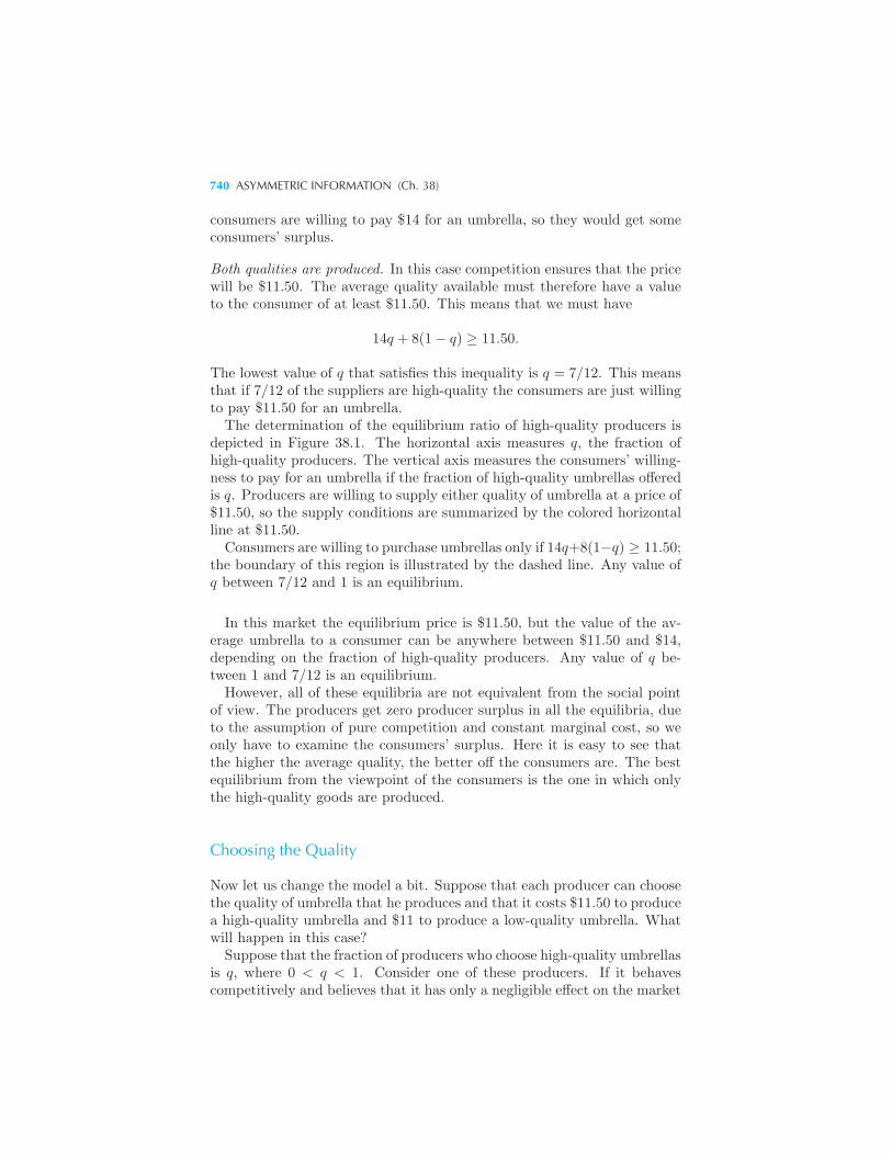
740 ASYMMETRIC INFORMATION (Ch. 38)
consumers are willing to pay $14 for an umbrella, so they would get someconsumers’ surplus.
Both qualities are produced. In this case competition ensures that the pricewill be $11.50. The average quality available must therefore have a valueto the consumer of at least $11.50. This means that we must have
14q + 8(1− q) ≥ 11.50.
The lowest value of q that satisfies this inequality is q = 7/12. This meansthat if 7/12 of the suppliers are high-quality the consumers are just willingto pay $11.50 for an umbrella.The determination of the equilibrium ratio of high-quality producers is
depicted in Figure 38.1. The horizontal axis measures q, the fraction ofhigh-quality producers. The vertical axis measures the consumers’ willing-ness to pay for an umbrella if the fraction of high-quality umbrellas offeredis q. Producers are willing to supply either quality of umbrella at a price of$11.50, so the supply conditions are summarized by the colored horizontalline at $11.50.Consumers are willing to purchase umbrellas only if 14q+8(1−q) ≥ 11.50;
the boundary of this region is illustrated by the dashed line. Any value ofq between 7/12 and 1 is an equilibrium.
In this market the equilibrium price is $11.50, but the value of the av-erage umbrella to a consumer can be anywhere between $11.50 and $14,depending on the fraction of high-quality producers. Any value of q be-tween 1 and 7/12 is an equilibrium.
However, all of these equilibria are not equivalent from the social pointof view. The producers get zero producer surplus in all the equilibria, dueto the assumption of pure competition and constant marginal cost, so weonly have to examine the consumers’ surplus. Here it is easy to see thatthe higher the average quality, the better off the consumers are. The bestequilibrium from the viewpoint of the consumers is the one in which onlythe high-quality goods are produced.
Choosing the Quality
Now let us change the model a bit. Suppose that each producer can choosethe quality of umbrella that he produces and that it costs $11.50 to producea high-quality umbrella and $11 to produce a low-quality umbrella. Whatwill happen in this case?Suppose that the fraction of producers who choose high-quality umbrellas
is q, where 0 < q < 1. Consider one of these producers. If it behavescompetitively and believes that it has only a negligible effect on the market
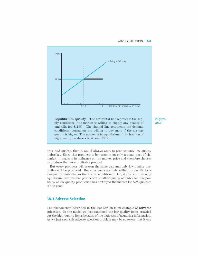
ADVERSE SELECTION 741
PRICE
FRACTION OF HIGH-QUALITY FIRMS1
11.50
p = 14 q + 8(1 – q)
7/12
Equilibrium quality. The horizontal line represents the sup-ply conditions: the market is willing to supply any quality ofumbrella for $11.50. The slanted line represents the demandconditions: consumers are willing to pay more if the averagequality is higher. The market is in equilibrium if the fraction ofhigh-quality producers is at least 7/12.
Figure38.1
price and quality, then it would always want to produce only low-qualityumbrellas. Since this producer is by assumption only a small part of themarket, it neglects its influence on the market price and therefore choosesto produce the more profitable product.
But every producer will reason the same way and only low-quality um-brellas will be produced. But consumers are only willing to pay $8 for alow-quality umbrella, so there is no equilibrium. Or, if you will, the onlyequilibrium involves zero production of either quality of umbrella! The pos-siblity of low-quality production has destroyed the market for both qualitiesof the good!
38.3 Adverse Selection
The phenomenon described in the last section is an example of adverseselection. In the model we just examined the low-quality items crowdedout the high-quality items because of the high cost of acquiring information.As we just saw, this adverse selection problem may be so severe that it can
742 ASYMMETRIC INFORMATION (Ch. 38)
completely destroy the market. Let’s consider a few other examples ofadverse selection.Consider first an example from the insurance industry. Suppose that
an insurance company wants to offer insurance for bicycle theft. They doa careful market survey and find that the incident of theft varies widelyacross communities. In some areas there is a high probability that a bicyclewill be stolen, and in other areas thefts are quite rare. Suppose that theinsurance company decides to offer the insurance based on the average theftrate. What do you think will happen?Answer: the insurance company is likely to go broke quickly! Think
about it. Who is going to buy the insurance at the average rate? Not thepeople in the safe communities—they don’t need much insurance anyway.Instead the people in the communities with a high incidence of theft willwant the insurance—they’re the ones who need it.But this means that the insurance claims will mostly be made by the
consumers who live in the high-risk areas. Rates based on the averageprobability of theft will be a misleading indication of the actual experi-ence of claims filed with the insurance company. The insurance companywill not get an unbiased selection of customers; rather they will get anadverse selection. In fact the term “adverse selection” was first used in theinsurance industry to describe just this sort of problem.It follows that in order to break even the insurance company must base
their rates on the “worst-case” forecasts and that consumers with a low,but not negligible, risk of bicycle theft will be unwilling to purchase theresulting high-priced insurance.A similar problem arises with health insurance—insurance companies
can’t base their rates on the average incidence of health problems in thepopulation. They can only base their rates on the average incidence ofhealth problems in the group of potential purchasers. But the people whowant to purchase health insurance the most are the ones who are likely toneed it the most and thus the rates must reflect this disparity.In such a situation it is possible that everyone can be made better off
by requiring the purchase of insurance that reflects the average risk in thepopulation. The high-risk people are better off because they can purchaseinsurance at rates that are lower than the actual risk they face and the low-risk people can purchase insurance that is more favorable to them than theinsurance offered if only high-risk people purchased it.A situation like this, where the market equilibrium is dominated by a
compulsary purchase plan, is quite surprising to most economists. Weusually think that “more choice is better,” so it is peculiar that restrictingchoice can result in a Pareto improvement. But it should be emphasizedthat this paradoxical result is due to the externality between the low-riskand high-risk people.In fact there are social institutions that help to solve this market ineffi-
ciency. It is commonly the case that employers offer health plans to their
MORAL HAZARD 743
employees as part of the package of fringe benefits. The insurance companycan base its rates on the averages over the set of employees and is assuredthat all employees must participate in the program, thus eliminating theadverse selection.
38.4 Moral Hazard
Another interesting problem that arises in the insurance industry is knownas the moral hazard problem. The term is somewhat peculiar, but thephenomenon is not hard to describe. Consider the bicycle-theft insurancemarket again and suppose for simplicity that all of the consumers live inareas with identical probabilities of theft, so that there is no problem ofadverse selection. On the other hand, the probability of theft may beaffected by the actions taken by the bicycle owners.For example, if the bicycle owners don’t bother to lock their bikes or use
only a flimsy lock, the bicycle is much more likely to be stolen than if theyuse a secure lock. Similar examples arise in other sorts of insurance. Inthe case of health insurance, for example, the consumers are less likely toneed the insurance if they take actions associated with a healthy lifestyle.We will refer to actions that affect the probability that some event occursas taking care.
When it sets its rates the insurance company has to take into accountthe incentives that the consumers have to take an appropriate amount ofcare. If no insurance is available consumers have an incentive to take themaximum possible amount of care. If it is impossible to buy bicycle-theftinsurance, then all bicyclists would use large expensive locks. In this casethe individual bears the full cost of his actions and accordingly he wantsto “invest” in taking care until the marginal benefit from more care justequals the marginal cost of doing so.But if a consumer can purchase bicycle insurance, then the cost inflicted
on the individual of having his bicycle stolen is much less. After all, if thebicycle is stolen then the person simply has to report it to the insurancecompany and he will get insurance money to replace it. In the extremecase, where the insurance company completely reimburses the individualfor the theft of his bicycle, the individual has no incentive to take care atall. This lack of incentive to take care is called moral hazard.Note the tradeoff involved: too little insurance means that people bear
a lot of risk, too much insurance means that people will take inadequatecare.If the amount of care is observable, then there is no problem. The insur-
ance company can base its rates on the amount of care taken. In real life itis common for insurance companies to give different rates to businesses thathave a fire sprinkler system in their building, or to charge smokers differentrates than nonsmokers for health insurance. In these cases the insurance
744 ASYMMETRIC INFORMATION (Ch. 38)
firm attempts to discriminate among users depending on the choices theyhave made that influence the probability of damage.
But insurance companies can’t observe all the relevant actions of thosethey insure. Therefore we will have the tradeoff described above: fullinsurance means too little care will be undertaken because the individualsdon’t face the full costs of their actions.
What does this imply about the types of insurance contracts that willbe offered? In general, the insurance companies will not want to offer theconsumers “complete” insurance. They will always want the consumer toface some part of the risk. This is why most insurance policies include a“deductible,” an amount that the insured party has to pay in any claim.By making the consumers pay part of a claim, the insurance companies canmake sure that the consumer always has an incentive to take some amountof care. Even though the insurance company would be willing to insurea consumer completely if they could verify the amount of care taken, thefact that the consumer can choose the amount of care he takes implies thatthe insurance company will not allow the consumer to purchase as muchinsurance as he wants if the company cannot observe the level of care.
This is also a paradoxical result when compared with the standard mar-ket analysis. Typically the amount of a good traded in a competitive marketis determined by the condition that demand equals supply—the marginalwillingness to pay equals the marginal willingness to sell. In the case ofmoral hazard, a market equilibrium has the property that each consumerwould like to buy more insurance, and the insurance companies would bewilling to provide more insurance if the consumers continued to take thesame amount of care . . . but this trade won’t occur because if the consumerswere able to purchase more insurance they would rationally choose to takeless care!
38.5 Moral Hazard and Adverse Selection
Moral hazard refers to situations where one side of the market can’t observethe actions of the other. For this reason it is sometimes called a hiddenaction problem.
Adverse selection refers to situations where one side of the market can’tobserve the “type” or quality of the goods on other side of the market. Forthis reason it is sometimes called a hidden information problem.
Equilibrium in a market involving hidden action typically involves someform of rationing—firms would like to provide more than they do, but theyare unwilling to do so since it will change the incentives of their customers.Equilibrium in a market involving hidden information will typically involvetoo little trade taking place because of the externality between the “good”and “bad” types.
SIGNALING 745
Equilibrium outcomes in this market appear to be inefficient, but one hasto be careful in making such a claim. The question to ask is “inefficientrelative to what?” The equilibrium will always be inefficient relative tothe equilibrium with full information. But this is of little help in makingpolicy decisions: if the firms in the industry find it too costly to collectmore information the government would probably find it too costly as well.The real question to ask is whether some sort of governmental interven-
tion in the market could improve efficiency even if the government had thesame information problems as the firms.In the case of hidden action considered above, the answer is usually
“no.” If the government can’t observe the care taken by the consumers,then it can do no better than the insurance companies. Of course thegovernment might have other tools at its disposal that are not available tothe insurance company—it could compel a particular level of care, and itcould set criminal punishments for those who did not take due care. But ifthe government can only set prices and quantities, then it can do no betterthan the private market can do.Similar issues arise in the case of hidden information. We have already
seen that if the government can compel people of all risk classes to purchaseinsurance, it is possible for everyone to be made better off. This is, on theface of it, a good case for intervention. On the other hand, there are costs togovernment intervention as well; economic decisions made by governmentaldecree may not be as cost-effective as those made by private firms. Justbecause there are governmental actions that can improve social welfaredoesn’t mean that these actions will be taken!Furthermore, there may be purely private solutions to the adverse selec-
tion problems. For example, we have already seen how providing healthinsurance as a fringe benefit can help to eliminate the adverse selectionproblem.
38.6 Signaling
Recall our model of the used-car market: the owners of the used cars knewthe quality, but the purchasers had to guess at the quality. We saw thatthis asymmetric information could cause problems in the market; in somecases, the adverse selection problem would result in too few transactionsbeing made.However, the story doesn’t end there. The owners of the good used cars
have an incentive to try to convey the fact that they have a good car tothe potential purchasers. They would like to choose actions that signalthe quality of their car to those who might buy it.One sensible signal in this context would be for the owner of a good used
car to offer a warranty. This would be a promise to pay the purchasersome agreed upon amount if the car turned out to be a lemon. Owners of
746 ASYMMETRIC INFORMATION (Ch. 38)
the good used cars can afford to offer such a warranty while the owners ofthe lemons can’t afford this. This is a way for the owners of the good usedcars to signal that they have good cars.
In this case signaling helps to make the market perform better. By offer-ing the warranty—the signal—the sellers of the good cars can distinguishthemselves from the sellers of the bad used cars. But there are other caseswhere signaling can make a market perform less well.
Let’s consider a very simplified model of the education market first ex-amined by Michael Spence.3 Suppose that we have two types of workers,able and unable. The able workers have a marginal product of a2, and theunable workers have a marginal product of a1, where a2 > a1. Supposethat a fraction b of the workers are able and 1− b of them are unable.
For simplicity we assume a linear production function so that the totaloutput produced by L2 able workers and L1 unable workers is a1L1+a2L2.We also assume a competitive labor market.
If worker quality is easily observable, then firms would just offer a wageof w2 = a2 to the able workers and of w1 = a1 to the unable workers. Thatis, each worker would be paid his marginal product and we would have anefficient equilibrium.
But what if the firm can’t observe the marginal products? If a firm can’tdistinguish the types of workers, then the best that it can do is to offer theaverage wage, which is w = (1−b)a1+ba2. As long as the good and the badworkers both agree to work at this wage there is no problem with adverseselection. And, given our assumption about the production function, thefirm produces just as much output and makes just as much profit as itwould if it could perfectly observe the type of the worker.
However, suppose now that there is some signal that the workers canacquire that will distinguish the two types. For example, suppose that theworkers can acquire education. Let e1 be the amount of education attainedby the type 1 workers and e2 the amount attained by the type 2 workers.Suppose that the workers have different costs of acquiring education, sothat the total cost of education for the able workers is c2e2 and the totalcost of education for the unable workers is c1e1. These costs are meant toinclude not only the dollar costs of attending school, but also includes theopportunity costs, the costs of the effort required, and so on.
Now we have two decisions to consider. The workers have to decide howmuch education to acquire and the firms have to decide how much to payworkers with different amounts of education. Let us make the extremeassumption that the education doesn’t affect worker productivity at all.Of course this isn’t true in real life—especially for economics courses—butit helps to keep the model simple.
3 Michael Spence, Market Signaling (Cambridge, Mass: Harvard University Press,1974).
SIGNALING 747
It turns out that the nature of the equilibrium in this model dependscrucially on the cost of acquiring education. Suppose that c2 < c1. Thissays that the marginal cost of acquiring education is less for the able workersthan the unable workers. Let e∗ be an education level that satisfies thefollowing inequalities:
a2 − a1c1
< e∗ <a2 − a1
c2.
Given our assumption that a2 > a1 and that c2 < c1 there must be suchan e∗.Now consider the following set of choices: the able workers all acquire
education level e∗ and the unable workers all acquire education level 0, andthe firm pays workers with education level e∗ a wage of a2 and workerswith less education than this a wage of a1. Note that the choice of theeducation level of a worker perfectly signals his type.But is this an equilibrium? Does anyone have an incentive to change
his or her behavior? Each firm is paying each worker his or her marginalproduct, so the firms have no incentive to do anything differently. Theonly question is whether the workers are behaving rationally given thewage schedule they face.Would it be in the interest of an unable worker to purchase education
level e∗? The benefit to the worker would be the increase in wages a2−a1.The cost to the unable worker would be c1e
∗. The benefits are less thanthe costs if
a2 − a1 < c1e∗.
But we are guaranteed that this condition holds by the choice of e∗. Hencethe unable workers find it optimal to choose a zero educational level.Is it actually in the interest of the able workers to acquire the level of
education e∗? The condition for the benefits to exceed the costs is
a2 − a1 > c2e∗,
and this condition also holds due to the choice of e∗.Hence this pattern of wages is indeed an equilibrium: if each able worker
chooses education level e∗ and each unable worker chooses a zero educa-tional level, then no worker has any reason to change his or her behavior.Due to our assumption about the cost differences, the education level ofa worker can, in equilibrium, serve as a signal of the different productivi-ties. This type of signaling equilibrium is sometimes called a separatingequilibrium since the equilibrium involves each type of worker making achoice that allows him to separate himself from the other type.Another possibility is a pooling equilibrium, in which each type of
worker makes the same choice. For example, suppose that c2 > c1, so thatthe able workers have a higher cost of acquiring education than the unable
748 ASYMMETRIC INFORMATION (Ch. 38)
workers. In this case it can be shown that the only equilibrium involvesthe workers all getting paid a wage based on their average ability, and sono signaling occurs.
The separating equilibrium is especially interesting since it is inefficientfrom a social point of view. Each able worker finds it in his interest to payfor acquiring the signal, even though it doesn’t change his productivityat all. The able workers want to acquire the signal not because it makesthem any more productive, but just because it distinguishes them from theunable workers. Exactly the same amount of output is produced in the(separating) signaling equilibrium as would be if there were no signalingat all. In this model the acquisition of the signal is a total waste from thesocial point of view.
It is worth thinking about the nature of this inefficiency. As before, itarises because of an externality. If both able and unable workers were paidtheir average product, the wage of the able workers would be depressedbecause of the presence of the unable workers. Thus they would have anincentive to invest in signals that will distinguish them from the less able.This investment offers a private benefit but no social benefit.
Of course signaling doesn’t always lead to inefficiencies. Some types ofsignals, such as the used-car warranties described above, help to facilitatetrade. In that case the equilibrium with signals is preferred to the equilib-rium without signals. So signaling can make things better or worse; eachcase has to be examined on its own merits.
EXAMPLE: The Sheepskin Effect
In the extreme form of the educational signaling model described aboveeducation has no effect on productivity: the years spent in school serveonly to signal the fixed ability of an individual. This is obviously an ex-aggeration: a student with 11 years of schooling almost certainly is moreproductive than one with 10 years of schooling due to the fact that he hasacquired more useful skills during the additional year. Presumably partof the returns to schooling are due to signaling, and part are due to theacquisition of useful skills while in school. How can we separate these twofactors?
Labor economists who have studied the returns to education have ob-served the following suggestive fact: the earnings of people who have grad-uated from high school are much higher than the incomes of people whohave only completed 3 years of high school. One study found that gradu-ating from high school increases earnings by 5 to 6 times as much as doescompleting a year in high school that does not result in graduation. Thesame discontinuous jump occurs for people who graduate from college. Ac-cording to one estimate, the economic return to the 16th year of schooling
INCENTIVES 749
are about three times as high as the return to the 15th year of schooling.4
If education imparts productive skills, we might well expect that peoplewith 11 years of education are paid more than people with 10 years ofeducation. What is surprising is that there is a huge jump in earningsassociated with high school graduation. Economists have termed this thesheepskin effect, in reference to the fact that diplomas were often writtenon sheepskins. Presumably, graduation from high school is some kind ofsignal. But what is it a signal of? In the educational signaling modeldescribed earlier, educational attainment was a signal of ability. Is thatwhat high school graduation signals? Or is it something else?Andrew Weiss, a Boston University economist, attempted to answer
these questions.5 He looked at a set of data describing how workers as-sembled equipment and was able to obtain a measure of how much outputthey produced in their first month on the job. He found that there wasa very small effect of education on output: each year of secondary educa-tion increased a worker’s output by about 1.3 percent. Furthermore, highschool graduates produced essentially the same amount of output as non-graduates. Apparently education contributed only a small amount to theinitial productivity of these workers.Weiss then looked at another data set that described various character-
istics of workers in a variety of occupations. He found that high schoolgraduates had significantly lower quit and absentee rates than nongrad-uates. It seems that high school graduates receive higher wages becausethey are more productive—but the reason that they are more productiveis because they stay with the firm longer and have fewer absences. Thissuggests that the signaling model does give us insight into real-world labormarkets. However, the actual signal sent by educational attainment is con-siderably more complex than the simplest version of the signaling modelsuggests.
38.7 Incentives
We turn now to a slightly different topic, the study of incentive sys-tems. As it turns out, our investigation of this topic will naturally involveasymmetric information. But it is useful to start with the case of fullinformation.The central question in the design of incentive systems is “How can I get
someone to do something for me?” Let’s pose this question in a specific
4 See Thomas Hungerford and Gary Solon, “Sheepskin Effects in the Returns to Edu-cation,” Review of Economics and Statistics, 69, 1987, 175–77.
5 “High School Graduation, Performance and Wages,” Journal of Political Economy,96, 4, 1988, 785–820.
750 ASYMMETRIC INFORMATION (Ch. 38)
context. Suppose that you own a plot of land but you are unable to workon the land yourself. So you try to hire someone to do the farming for you.What sort of compensation system should you set up?One plan might involve paying the worker a lump-sum fee independent of
how much he produces. But then he would have little incentive to work. Ingeneral a good incentive plan will make the payment of the worker dependin some way on the output he produces. The problem of incentive design isto determine exactly how sensitive the payment should be to the producedoutput.Let x be the amount of “effort” that the worker expends, and let y = f(x)
be the amount of output produced; for simplicity we suppose that the priceof output is 1 so that y also measures the value of the output. Let s(y)be the amount that you pay the worker if he produces y dollars worth ofoutput. Presumably you would like to choose the function s(y) to maximizeyour profits y − s(y).
What are the constraints that you face? In order to answer this questionwe have to look at things from the worker’s perspective.We assume that the worker finds effort costly, and write c(x) for the
cost of effort x. We assume that this cost function has the usual shape:both total and marginal costs increase as effort increases. The utility of theworker who chooses effort level x is then simply s(y)−c(x) = s(f(x))−c(x).The worker may have other alternatives available that give him some utilityu. This could come from working at other jobs or from not working at all.All that is relevant for the design of the incentive scheme is that the utilitythat the worker gets from this job must be at least as great as the utilityhe could get elsewhere. This gives us the participation constraint:
s(f(x))− c(x) ≥ u.
Given this constraint we can determine how much output we can getfrom the worker. You want to induce the worker to choose an effort levelx that yields you the greatest surplus given the constraint that the workeris willing to work for you:
maxx
f(x)− s(f(x))
such that s(f(x))− c(x) ≥ u.
In general, you will want the worker to choose x to just satisfy the constraintso that s(f(x)) − c(x) = u. Substituting this into the objective functionwe have the unconstrained maximization problem
maxx
f(x)− c(x)− u.
But it is easy to solve this problem! Just choose x∗ so that the marginalproduct equals the marginal cost:
MP (x∗) = MC(x∗).
INCENTIVES 751
Any choice of x∗ where the marginal benefit is not equal to the marginalcost cannot maximize profits.This tells us what level of effort the owner wants to achieve; now we have
to ask what he has to pay the worker to achieve that effort. That is, whatdoes the function s(y) have to look like to induce the worker to choose tomake x∗ the optimal choice?Suppose that you decide that you want to induce the worker to put in
x∗ amount of effort. Then you must make it in his interest to do so; thatis, you must design your incentive scheme s(y) so that the utility fromchoosing to work x∗ is larger than the utility of worker any other amountx. This gives us the constraint
s(f(x∗))− c(x∗) ≥ s(f(x))− c(x) for all x.
This constraint is called the incentive compatibility constraint. Itsimply says that the utility to the worker from choosing x∗ must be greaterthan the utility of any other choice of effort.So we have two conditions that the incentive scheme must satisfy: first,
it must give total utility to the worker of u, and second, it must make themarginal product of effort equal to the marginal cost of effort at the effortlevel x∗. There are several ways to do this.
Rent. The landowner could simply rent the land to the worker for someprice R, so that the worker gets all the output he produces after he paysthe owner R. For this scheme
s(f(x)) = f(x)−R.
If the worker maximizes s(f(x)) − c(x) = f(x) − R − c(x), he will choosethe effort level where MP (x∗) = MC(x∗), which is exactly what the ownerwants. The rental rate R is determined from the participation condition.Since the total utility to the worker must be u we have
f(x∗)− c(x∗)−R = u,
which says R = f(x∗)− c(x∗)− u.
Wage labor. In this scheme the landowner pays the worker a constant wageper unit of effort along with a lump sum K. This means that the incentivepayment takes the form
s(x) = wx+K.
The wage rate w is equal to the marginal product of the worker at the opti-mal choice x∗, MP (x∗). The constant K is chosen to just make the workerindifferent between working for the landowner and working elsewhere; thatis, it is chosen to satisfy the participation constraint.
752 ASYMMETRIC INFORMATION (Ch. 38)
The problem of maximizing s(f(x))− c(x) then becomes
maxx
wx+K − c(x),
which means that the worker will choose x so as to set his marginal costequal to the wage: w = MC(x). Since the wage isMP (x∗), this means thatthe optimal choice of the worker will be x∗ such that MP (x∗) = MC(x∗)which is just what the firm wants.
Take-it-or-leave-it. In this scheme the landowner pays the worker B∗ ifhe works x∗ and zero otherwise. The amount B∗ is determined by theparticipation constraint B∗ − c(x∗) = u, so B∗ = u + c(x∗). If the workerchooses any level of effort x �= x∗, he gets a utility of −c(x). If he choosesx∗, he gets a utility of u. Hence the optimal choice for the worker is to setx = x∗.
Each of these schemes is equivalent as far as the analysis goes: each onegives the worker a utility of u, and each one gives the worker an incentive towork the optimal amount x∗. At this level of generality there is no reasonto choose between them.If all of these schemes are optimal, what could a nonoptimal scheme look
like? Here is an example.
Sharecropping. In sharecropping the worker and the landowner each getsome fixed percentage of the output. Suppose that the worker’s share takesthe form s(x) = αf(x) + F , where F is some constant and α < 1. This isnot an efficient scheme for the problem under consideration. It is easy tosee why. The worker’s maximization problem is
maxx
αf(x) + F − c(x),
which means that he would choose a level of effort x where
αMP (x) = MC(x).
Such an effort level clearly cannot satisfy the efficiency condition thatMP (x) = MC(x).
Here is a way to summarize this analysis. In order to design an efficientincentive scheme it is necessary to ensure that the person who makes theeffort decision is the residual claimant to the output. The way the ownercan make himself as well off as possible is to make sure that he gets theworker to produce the optimal amount of output. This is the output levelwhere the marginal product of the worker’s extra effort equals the marginalcost of putting forth that effort. It follows that the incentive scheme mustprovide a marginal benefit to the worker equal to his marginal product.
INCENTIVES 753
EXAMPLE: Voting Rights in the Corporation
Normally shareholders in a corporation have the right to vote on variousissues related to the management of the corporation while bondholders donot. Why is this? The answer comes from looking at the structure of payoffsto stockholders and bondholders. If a corporation produces X dollars ofprofit in a given years, the bondholders have first claim on these profits,while the amount that is left over goes to the stockholders. If the total claimby the bondholders is B, then the amount that goes to the stockholders isX −B. This makes the stockholders the residual claimants—so they havean incentive to make X as large as possible. The bondholders on the otherhand only have an incentive to make sure that X is at least B, since that isthe most that they are entitled to. Hence giving the stockholders the rightto make decisions will generally result in larger profits.
EXAMPLE: Chinese Economic Reforms
Prior to 1979 Chinese rural communes were organized along orthodoxMarxist lines. Workers were paid according to a rough estimate of howmuch they contributed to the commune income. Five percent of the com-mune’s land was set aside for private plots, but peasants were not allowedto travel to cities to sell the output from their private farms. All trade hadto take place through a highly regulated government market.
At the end of 1978 the Chinese central government instituted a majorreform in the structure of agriculture, known as the “responsibility system.”In the responsibility system, any production in excess of a fixed quotawas kept by the household and could be sold on private markets. Thegovernment removed restrictions on private plots and increased the amountof land devoted to private farming. By the end of 1984, 97 percent of thefarmers operated under this responsibility system.
Note that the structure of the system is very much like the optimal in-centive mechanism described above: each household makes a lump-sumpayment to the commune but can keep anything in excess of this quota.Hence the marginal incentives for household production are the economi-cally appropriate ones.
The effect of this new system on agricultural output was phenomenal:between 1978 and 1984, the output of Chinese agriculture increased by over61 percent! However, not all of this increase is due to better incentives; atthe same time these reforms were going on, the Chinese government alsochanged the controlled prices of agricultural goods, and even allowed someof these prices to be determined on private markets.
Three economists attempted to divide the increase in output into the part
754 ASYMMETRIC INFORMATION (Ch. 38)
due to better incentives and the part due to the change in prices.6 Theyfound that over three-fourths of the increase was due to the improvementin incentives, and only one-fourth was due to the price reforms.
38.8 Asymmetric Information
The above analysis provides some insights about the use of different sortsof incentive schemes. For example, it shows that renting the land to aworker is better than sharecropping. But this really proves too much. Ifour analysis is a good description of the world, then we would expect tosee rental or wage labor used in agriculture and never see sharecroppingused, except by mistake.Clearly this isn’t right. Sharecropping has been used for thousands of
years in some parts of the world, so it is likely that it fulfills some kind ofneed. What have we left out of our model?Given the title of this section it is not hard to guess the answer: we’ve
left out problems involving imperfect information. We assumed that theowner of the firm could perfectly observe the effort of the worker. In manysituations of interest it may be impossible to observe the effort. At best theowner may observe some signal of the effort such as the resulting productionof output. The amount of output produced by a farmer may depend inpart on his effort, but it may also depend on the weather, the quality ofthe inputs, and many other factors. Because of this kind of “noise,” apayment from the owner to the worker based on output will not in generalbe equivalent to a payment based on effort alone.This is essentially a problem of asymmetric information: the worker can
choose his effort level, but the owner cannot perfectly observe it. Theowner has to guess the effort from the observed output, and the design ofthe optimal incentive scheme has to reflect this inference problem.Consider the four incentive schemes described above. What goes wrong
if effort is not perfectly correlated with output?
Rent. If the firm rents the technology to the worker, then the worker canget all of the output that remains after paying the fixed rental fee. If outputhas a random component, this means that the worker will have to bear allthe risk from the random factors. If the worker is more risk averse thanthe owner—which is the likely case—this will be inefficient. In general, theworker would be willing to give up some of the residual profits in order tohave a less risky income stream.
6 J. McMillan, J. Whalley, and L. Zhu, “The Impact of China’s Economic Reformson Agricultural Productivity Growth,” Journal of Political Economy, 97, 4, 1989,781–807.
ASYMMETRIC INFORMATION 755
Wage labor. The problem with wage labor is that it requires observationof the amount of labor input. The wage has to be based on the effort putin to production, not just the hours spent in the firm. If the owner can’tobserve the amount of labor input, then it will be impossible to implementthis kind of incentive scheme.
Take-it-or-leave-it. If the incentive payment is based on the labor input,then we have the same problem with this scheme as with wage labor. If thepayment is based on output, then the scheme involves the worker bearingall the risk. Even missing the “target output” by a small amount resultsin a zero payment.
Sharecropping. This is something of a happy medium. The payment to theworker depends in part on observed output, but the worker and the ownershare the risk of output fluctuations. This gives the worker an incentive toproduce output but it doesn’t leave him bearing all the risk.
The introduction of asymmetric information has made a drastic changein our evaluation of the incentive methods. If the owner can’t observe effort,then wage labor is infeasible. Rent and the take-it-or-leave-it scheme leavethe worker bearing too much risk. Sharecropping is a compromise betweenthe two extremes: it gives the worker some incentive to produce, but itdoesn’t leave him with all the risk.
EXAMPLE: Monitoring Costs
It is not always easy to observe the amount of effort an employee puts intohis or her job. Consider, for example, a job as a clerk in a 24-hour con-venience store. How can the manager observe the employees’ performancewhen the manager isn’t around? Even if there are ways to observe thephysical output of the employee (shelves stocked, sales rung up) it is muchharder to observe things like politeness to customers.There is little doubt that some of the worst service in the world was
provided in the formerly Communist countries in Eastern Europe: onceyou managed to attract the attention of a clerk, you were more likely to begreeted by a scowl than a smile. Nevertheless, a Hungarian entrepreneur,Gabor Varszegi, has made millions by providing high-quality service in hisphoto developing shops in Budapest.7
Varszegi says that he got his start as a businessman in the mid-sixtiesby playing bass guitar and managing a rock group. “Back then,” he says,“the only private businessmen in Eastern Europe were rock musicians.”
7 See Steven Greenhouse, “A New Formula in Hungary: Speed Service and Grow Rich,”New York Times, June 5, 1990, A1.
756 ASYMMETRIC INFORMATION (Ch. 38)
He introduced one-hour film developing to Hungary in 1985; the next bestalternative to his one-hour developing shops was the state-run agency thattook one month.Varszegi follows two rules in labor relations: he never hires anyone who
worked under Communism, and he pays his workers four times the marketwage. This makes perfect sense in light of the above remarks about mon-itoring costs: there are very few employees per store and monitoring theirbehavior is very costly. If there were only a small penalty to being fired,there would be great temptation to slack off. By paying the workers muchmore than they could get elsewhere, Varszegi makes it very costly for themto be fired—and reduces his monitoring costs significantly.
EXAMPLE: The Grameen Bank
A village moneylender in Bangladesh charges over 150 percent interest ayear. Any American banker would love a return of that size: why isn’tCitibank installing money machines in Bangladesh? To ask the question isto answer it: Citibank would probably not do as well as the moneylender.The village moneylender has a comparative advantage in these small-scaleloans for several reasons.
• The village moneylender can deal more effectively with the small scale oflending involved;
• The moneylender has better access to information about who are goodand bad credit risks than an outsider does.
• The moneylender is in a better position to monitor the progress of theloan payments to insure repayment.
These three problems—returns to scale, adverse selection and moralhazard—allow the village moneylender to maintain a local monopoly inthe credit market.Such a local monopoly is especially pernicious in an underdeveloped
country such as Bangladesh. At an interest rate of 150 percent there aremany profitable projects that are not being undertaken by the peasants.Improved access to credit could lead to a major increase in investment, anda corresponding increase in the standards of living.Muhammad Yunus, an American-trained economist from Bangladesh,
has developed an ingenious institution known as the Grameen Bank (vil-lage bank) to address some of these problems. In the Grameen plan, en-trepreneurs with separate projects get together and apply for a loan as agroup. If the loan is approved, two members of the group get their loanand commence their investment activity. If they are successful in meeting
SUMMARY 757
the repayment schedule, two more members get loans. If they are alsosuccessful the last member, the group leader, will get a loan.The Grameen bank addresses each of the three problems described above.
Since the quality of the group influences whether or not individual memberswill get loans, potential members are highly selective about who they willjoin with. Since members of the group can only get loans if other memberssucceed in their investments, there are strong incentives to help each otherout and share expertise. Finally, these activities of choosing candidates forloans and monitoring the progress of the repayments are all done by thepeasants themselves, not directly by the loan officers at the bank.The Grameen bank has been very successful. It makes about 475,000
loans a month with an average size of $70. Their loan-recovery rate isabout 98 percent, while conventional lenders in Bangladesh achieve a loan-recovery rate of about 30 to 40 percent. The success of the group respon-sibility program in encouraging investment has led to its adoption in anumber of other poverty-stricken areas in North and South America.
Summary
1. Imperfect and asymmetric information can lead to drastic differences inthe nature of market equilbrium.
2. Adverse selection refers to situations where the type of the agents is notobservable so that one side of the market has to guess the type or qualityof a product based on the behavior of the other side of the market.
3. In markets involving adverse selection too little trade may take place.In this case it is possible that everyone can be made better off by forcingthem to transact.
4. Moral hazard refers to a situation where one side of the market can’tobserve the actions of the other side.
5. Signaling refers to the fact that when adverse selection or moral hazardare present some agents will want to invest in signals that will differentiatethem from other agents.
6. Investment in signals may be privately beneficial but publically wasteful.On the other hand, investment in signals may help to solve problems dueto asymmetric information.
7. Efficient incentive schemes (with perfect observability of effort) leave theworker as the residual claimant. This means that the worker will equatemarginal benefits and marginal costs.

758 ASYMMETRIC INFORMATION (Ch. 38)
8. But if information is imperfect this is no longer true. In general, anincentive scheme that shares risks as well as providing incentives will beappropriate.
REVIEW QUESTIONS
1. Consider the model of the used-car market presented in this chapter.What is the maximum amount of consumers’ surplus that is created bytrade in the market equilibrium?
2. In the same model, how much consumers’ surplus would be createdby randomly assigning buyers to sellers? Which method gives the largersurplus?
3. A worker can produce x units of output at a cost of c(x) = x2/2. Hecan achieve a utility level of u = 0 working elsewhere. What is the optimalwage-labor incentive scheme s(x) for this worker?
4. Given the setup of the previous problem, what would the worker bewilling to pay to rent the production technology?
5. How would your answer to the last problem change if the worker’s alter-native employment gave him u = 1?
MATHEMATICALAPPENDIX
In this Appendix we will provide a brief review of some of the mathematicalconcepts that are used in the text. This material is meant to serve as areminder of the definitions of various terms used in the text. It is emphat-ically not a tutorial in mathematics. The definitions given will generallybe the simplest, not the most rigorous.
A.1 Functions
A function is a rule that describes a relationship between numbers. Foreach number x, a function assigns a unique number y according to somerule. Thus a function can be indicated by describing the rule, as “take anumber and square it,” or “take a number and multiply it by 2,” and soon. We write these particular functions as y = x2, y = 2x. Functions aresometimes referred to as transformations.Often we want to indicate that some variable y depends on some other
variable x, but we don’t know the specific algebraic relationship between thetwo variables. In this case we write y = f(x), which should be interpretedas saying that the variable y depends on x according to the rule f .Given a function y = f(x), the number x is often called the indepen-
dent variable, and the number y is often called the dependent variable.
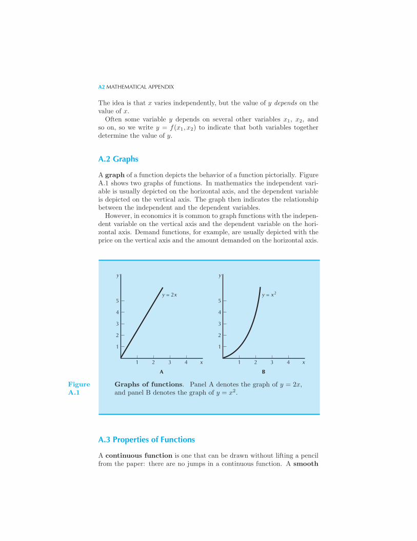
A2 MATHEMATICAL APPENDIX
The idea is that x varies independently, but the value of y depends on thevalue of x.Often some variable y depends on several other variables x1, x2, and
so on, so we write y = f(x1, x2) to indicate that both variables togetherdetermine the value of y.
A.2 Graphs
A graph of a function depicts the behavior of a function pictorially. FigureA.1 shows two graphs of functions. In mathematics the independent vari-able is usually depicted on the horizontal axis, and the dependent variableis depicted on the vertical axis. The graph then indicates the relationshipbetween the independent and the dependent variables.However, in economics it is common to graph functions with the indepen-
dent variable on the vertical axis and the dependent variable on the hori-zontal axis. Demand functions, for example, are usually depicted with theprice on the vertical axis and the amount demanded on the horizontal axis.
5
4
3
2
1
y
x1 2 3 4
A
5
4
3
2
1
y
x1 2 3 4
B
y = 2x y = x2
FigureA.1
Graphs of functions. Panel A denotes the graph of y = 2x,and panel B denotes the graph of y = x2.
A.3 Properties of Functions
A continuous function is one that can be drawn without lifting a pencilfrom the paper: there are no jumps in a continuous function. A smooth
EQUATIONS AND IDENTITIES A3
function is one that has no “kinks” or corners. A monotonic functionis one that always increases or always decreases; a positive monotonicfunction always increases as x increases, while a negative monotonicfunction always decreases as x increases.
A.4 Inverse Functions
Recall that a function has the property that for each value of x there isa unique value of y associated with it and that a monotonic function isone that is always increasing or always decreasing. This implies that for amonotonic function there will be a unique value of x associated with eachvalue of y.We call the function that relates x to y in this way an inverse function.
If you are given y as a function of x, you can calculate the inverse functionjust by solving for x as a function of y. If y = 2x, then the inverse functionis x = y/2. If y = x2, then there is no inverse function; given any y, bothx = +
√y and x = −√
y have the property that their square is equal to y.Thus there is not a unique value of x associated with each value of y, as isrequired by the definition of a function.
A.5 Equations and Identities
An equation asks when a function is equal to some particular number.Examples of equations are
2x = 8
x2 = 9
f(x) = 0.
The solution to an equation is a value of x that satisfies the equation.The first equation has a solution of x = 4. The second equation has twosolutions, x = 3 and x = −3. The third equation is just a general equation.We don’t know its solution until we know the actual rule that f stands for,but we can denote its solution by x∗. This simply means that x∗ is a numbersuch that f(x∗) = 0. We say that x∗ satisfies the equation f(x) = 0.An identity is a relationship between variables that holds for all values
of the variables. Here are some examples of identities:
(x+ y)2 ≡ x2 + 2xy + y2
2(x+ 1) ≡ 2x+ 2.
The special symbol ≡ means that the left-hand side and the right-handside are equal for all values of the variables. An equation only holds forsome values of the variables, whereas an identity is true for all values of thevariables. Often an identity is true by the definition of the terms involved.
A4 MATHEMATICAL APPENDIX
A.6 Linear Functions
A linear function is a function of the form
y = ax+ b,
where a and b are constants. Examples of linear functions are
y = 2x+ 3
y = x− 99.
Strictly speaking, a function of the form y = ax + b should be called anaffine function, and only functions of the form y = ax should be calledlinear functions. However, we will not insist on this distinction.Linear functions can also be expressed implicitly in forms like ax+by = c.
In such a case, we often like to solve for y as a function of x to convert thisto the “standard” form:
y =c
b− a
bx.
A.7 Changes and Rates of Change
The notation Δx is read as “the change in x.” It does not mean Δ timesx. If x changes from x∗ to x∗∗, then the change in x is just
Δx = x∗∗ − x∗.
We can also writex∗∗ = x∗ +Δx
to indicate that x∗∗ is x∗ plus a change in x.Typically Δx will refer to a small change in x. We sometimes express
this by saying that Δx represents a marginal change.A rate of change is the ratio of two changes. If y is a function of x
given by y = f(x), then the rate of change of y with respect to x is denotedby
Δy
Δx=
f(x+Δx)− f(x)
Δx.
The rate of change measures how y changes as x changes.A linear function has the property that the rate of change of y with
respect to x is constant. To prove this, note that if y = a+ bx, then
Δy
Δx=
a+ b(x+Δx)− a− bx
Δx=
bΔx
Δx= b.
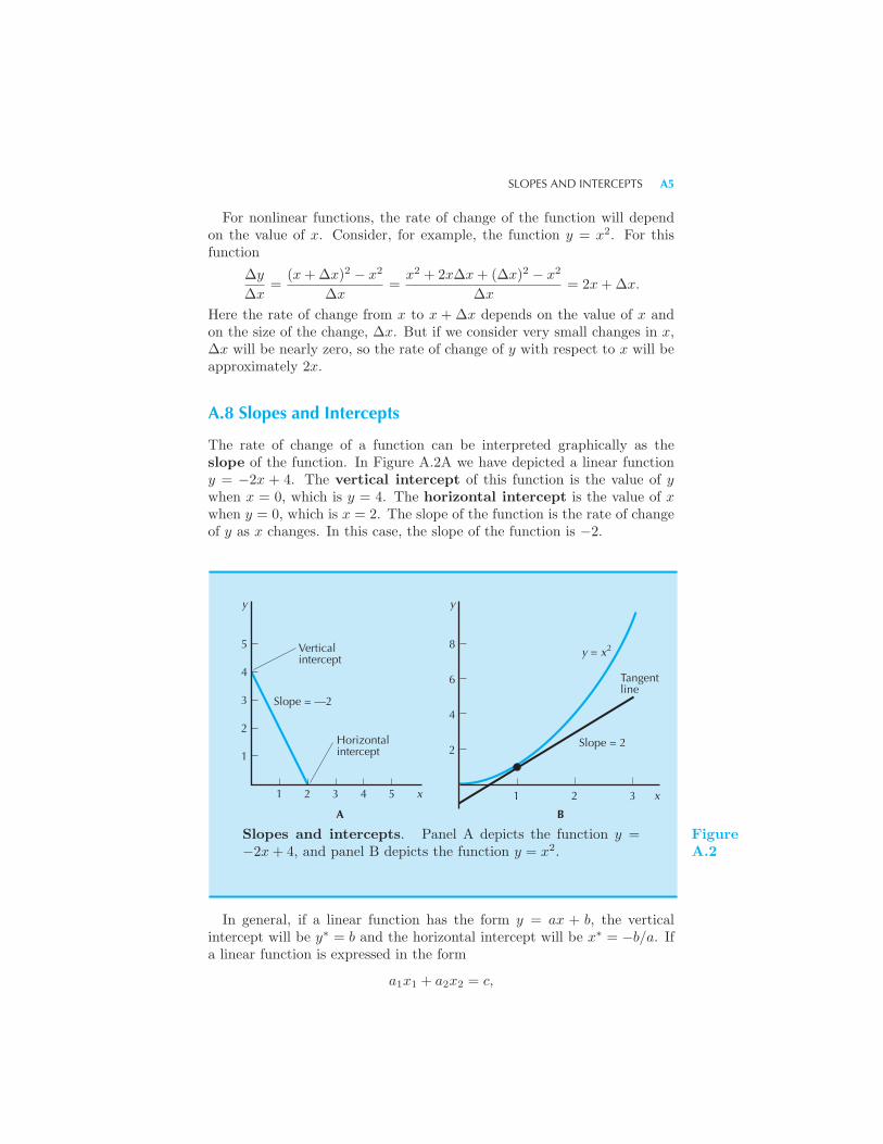
SLOPES AND INTERCEPTS A5
For nonlinear functions, the rate of change of the function will dependon the value of x. Consider, for example, the function y = x2. For thisfunction
Δy
Δx=
(x+Δx)2 − x2
Δx=
x2 + 2xΔx+ (Δx)2 − x2
Δx= 2x+Δx.
Here the rate of change from x to x + Δx depends on the value of x andon the size of the change, Δx. But if we consider very small changes in x,Δx will be nearly zero, so the rate of change of y with respect to x will beapproximately 2x.
A.8 Slopes and Intercepts
The rate of change of a function can be interpreted graphically as theslope of the function. In Figure A.2A we have depicted a linear functiony = −2x + 4. The vertical intercept of this function is the value of ywhen x = 0, which is y = 4. The horizontal intercept is the value of xwhen y = 0, which is x = 2. The slope of the function is the rate of changeof y as x changes. In this case, the slope of the function is −2.
5
4
3
2
1
y
x
Slope = —2
Horizontalintercept
Verticalintercept
1 2 3 4 5
A
y
Slope = 2
8
6
4
2
B
21 3 x
Tangentline
y = x2
Slopes and intercepts. Panel A depicts the function y =−2x+ 4, and panel B depicts the function y = x2.
FigureA.2
In general, if a linear function has the form y = ax + b, the verticalintercept will be y∗ = b and the horizontal intercept will be x∗ = −b/a. Ifa linear function is expressed in the form
a1x1 + a2x2 = c,
A6 MATHEMATICAL APPENDIX
then the horizontal intercept will be the value of x1 when x2 = 0, which isx∗1 = c/a1, and the vertical intercept will occur when x1 = 0, which means
x∗2 = c/a2. The slope of this function is −a1/a2.A nonlinear function has the property that its slope changes as x changes.
A tangent to a function at some point x is a linear function that has thesame slope. In Figure A.2B we have depicted the function x2 and thetangent line at x = 1.
If y increases whenever x increases, then Δy will always have the samesign as Δx, so that the slope of the function will be positive. If on theother hand y decreases when x increases, or y increases when x decreases,Δy and Δx will have opposite signs, so that the slope of the function willbe negative.
A.9 Absolute Values and Logarithms
The absolute value of a number is a function f(x) defined by the followingrule:
f(x) ={
x if x ≥ 0−x if x < 0.
Thus the absolute value of a number can be found by dropping the sign ofthe number. The absolute value function is usually written as |x|.The (natural) logarithm or log of x describes a particular function of
x, which we write as y = lnx or y = ln(x). The logarithm function is theunique function that has the properties
ln(xy) = ln(x) + ln(y)
for all positive numbers x and y and
ln(e) = 1.
(In this last equation, e is the base of natural logarithms which is equal to2.7183 . . .) In words, the log of the product of two numbers is the sum ofthe individual logs. This property implies another important property oflogarithms:
ln(xy) = yln(x),
which says that the log of x raised to the power y is equal to y times thelog of x.
A.10 Derivatives
The derivative of a function y = f(x) is defined to be
df(x)
dx= lim
Δx→0
f(x+Δx)− f(x)
Δx.
SECOND DERIVATIVES A7
In words, the derivative is the limit of the rate of change of y with respectto x as the change in x goes to zero. The derivative gives precise meaningto the phrase “the rate of change of y with respect to x for small changesin x.” The derivative of f(x) with respect to x is also denoted by f ′(x).
We have already seen that the rate of change of a linear function y =ax+ b is constant. Thus for this linear function
df(x)
dx= a.
For a nonlinear function the rate of change of y with respect to x willusually depend on x. We saw that in the case of f(x) = x2, we hadΔy/Δx = 2x+Δx. Applying the definition of the derivative
df(x)
dx= lim
Δx→02x+Δx = 2x.
Thus the derivative of x2 with respect to x is 2x.It can be shown by more advanced methods that if y = lnx, then
df(x)
dx=
1
x.
A.11 Second Derivatives
The second derivative of a function is the derivative of the derivative ofthat function. If y = f(x), the second derivative of f(x) with respect to xis written as d2f(x)/dx2 or f ′′(x). We know that
d(2x)
dx= 2
d(x2)
dx= 2x.
Thusd2(2x)
dx2=
d(2)
dx= 0
d2(x2)
dx2=
d(2x)
dx= 2.
The second derivative measures the curvature of a function. A functionwith a negative second derivative at some point is concave near that point;its slope is decreasing. A function with a positive second derivative at apoint is convex near that point; its slope is increasing. A function with azero second derivative at a point is flat near that point.
A8 MATHEMATICAL APPENDIX
A.12 The Product Rule and the Chain Rule
Suppose that g(x) and h(x) are both functions of x. We can define thefunction f(x) that represents their product by f(x) = g(x)h(x). Then thederivative of f(x) is given by
df(x)
dx= g(x)
dh(x)
dx+ h(x)
dg(x)
dx.
Given two functions y = g(x) and z = h(y), the composite function is
f(x) = h(g(x)).
For example, if g(x) = x2 and h(y) = 2y + 3, then the composite functionis
f(x) = 2x2 + 3.
The chain rule says that the derivative of a composite function, f(x),with respect to x is given by
df(x)
dx=
dh(y)
dy
dg(x)
dx.
In our example, dh(y)/dy = 2, and dg(x)/dx = 2x, so the chain rule saysthat df(x)/dx = 2 × 2x = 4x. Direct calculation verifies that this is thederivative of the function f(x) = 2x2 + 3.
A.13 Partial Derivatives
Suppose that y depends on both x1 and x2, so that y = f(x1, x2). Thenthe partial derivative of f(x1, x2) with respect to x1 is defined by
∂f(x1, x2)
∂x1= lim
Δx1→0
f(x1 +Δx1, x2)− f(x1, x2)
Δx1.
The partial derivative of f(x1, x2) with respect to x1 is just the derivativeof the function with respect to x1, holding x2 fixed. Similarly, the partialderivative with respect to x2 is
∂f(x1, x2)
∂x2= lim
Δx2→0
f(x1, x2 +Δx2)− f(x1, x2)
Δx2.
Partial derivatives have exactly the same properties as ordinary derivatives;only the name has been changed to protect the innocent (that is, peoplewho haven’t seen the ∂ symbol).
OPTIMIZATION A9
In particular, partial derivatives obey the chain rule, but with an extratwist. Suppose that x1 and x2 both depend on some variable t and thatwe define the function g(t) by
g(t) = f(x1(t), x2(t)).
Then the derivative of g(t) with respect to t is given by
dg(t)
dt=
∂f(x1, x2)
∂x1
dx1(t)
dt+
∂f(x1, x2)
∂x2
dx2(t)
dt.
When t changes, it affects both x1(t) and x2(t). Therefore, we need tocalculate the derivative of f(x1, x2) with respect to each of those changes.
A.14 Optimization
If y = f(x), then f(x) achieves a maximum at x∗ if f(x∗) ≥ f(x) forall x. It can be shown that if f(x) is a smooth function that achieves itsmaximum value at x∗, then
df(x∗)
dx= 0
d2f(x∗)
dx2≤ 0.
These expressions are referred to as the first-order condition and thesecond-order condition for a maximum. The first-order condition saysthat the function is flat at x∗, while the second-order condition says thatthe function is concave near x∗. Clearly both of these properties have tohold if x∗ is indeed a maximum.We say that f(x) achieves its minimum value at x∗ if f(x∗) ≤ f(x) for
all x. If f(x) is a smooth function that achieves its minimum at x∗, then
df(x∗)
dx= 0
d2f(x∗)
dx2≥ 0.
The first-order condition again says that the function is flat at x∗, whilethe second-order condition now says that the function is convex near x∗.
If y = f(x1, x2) is a smooth function that achieves its maximum orminimum at some point (x∗
1, x∗2), then we must satisfy
∂f(x∗1, x
∗2)
∂x1= 0
∂f(x∗1, x
∗2)
∂x2= 0.
These are referred to as the first-order conditions. There are also second-order conditions for this problem, but they are more difficult to describe.
A10 MATHEMATICAL APPENDIX
A.15 Constrained Optimization
Often we want to consider the maximum or minimum of some function oversome restricted values of (x1, x2). The notation
maxx1,x2
f(x1, x2)
such that g(x1, x2) = c.
means
find x∗1 and x∗
2 such that f(x∗1, x
∗2) ≥ f(x1, x2) for all values of x1 and x2
that satisfy the equation g(x1, x2) = c.
The function f(x1, x2) is called the objective function, and the equa-tion g(x1, x2) = c is called the constraint. Methods for solving this kindof constrained maximization problem are described in the Appendix toChapter 5.
ANSWERS
1 The Market
1.1. It would be constant at $500 for 25 apartments and then drop to $200.
1.2. In the first case, $500, and in the second case, $200. In the third case,the equilibrium price would be any price between $200 and $500.
1.3. Because if we want to rent one more apartment, we have to offer a lowerprice. The number of people who have reservation prices greater than pmust always increase as p decreases.
1.4. The price of apartments in the inner ring would go up since demandfor apartments would not change but supply would decrease.
1.5. The price of apartments in the inner ring would rise.
1.6. A tax would undoubtedly reduce the number of apartments suppliedin the long run.
1.7. He would set a price of 25 and rent 50 apartments. In the second casehe would rent all 40 apartments at the maximum price the market wouldbear. This would be given by the solution to D(p) = 100− 2p = 40, whichis p∗ = 30.
1.8. Everyone who had a reservation price higher than the equilibriumprice in the competitive market, so that the final outcome would be Paretoefficient. (Of course in the long run there would probably be fewer newapartments built, which would lead to another kind of inefficiency.)
2 Budget Constraint
2.1. The new budget line is given by 2p1x1 + 8p2x2 = 4m.
2.2. The vertical intercept (x2 axis) decreases and the horizontal intercept(x1 axis) stays the same. Thus the budget line becomes flatter.
A12 ANSWERS
2.3. Flatter. The slope is −2p1/3p2.
2.4. A good whose price has been set to 1; all other goods’ prices aremeasured relative to the numeraire good’s price.
2.5. A tax of 8 cents a gallon.
2.6. (p1 + t)x1 + (p2 − s)x2 = m− u.
2.7. Yes, since all of the bundles the consumer could afford before areaffordable at the new prices and income.
3 Preferences
3.1. No. It might be that the consumer was indifferent between the twobundles. All we are justified in concluding is that (x1, x2) � (y1, y2).
3.2. Yes to both.
3.3. It is transitive, but it is not complete—two people might be the sameheight. It is not reflexive since it is false that a person is strictly taller thanhimself.
3.4. It is transitive, but not complete. What if A were bigger but slowerthan B? Which one would he prefer?
3.5. Yes. An indifference curve can cross itself, it just can’t cross anotherdistinct indifference curve.
3.6. No, because there are bundles on the indifference curve that havestrictly more of both goods than other bundles on the (alleged) indifferencecurve.
3.7. A negative slope. If you give the consumer more anchovies, you’vemade him worse off, so you have to take away some pepperoni to get himback on his indifference curve. In this case the direction of increasing utilityis toward the origin.
3.8. Because the consumer weakly prefers the weighted average of two bun-dles to either bundle.
3.9. If you give up one $5 bill, how many $1 bills do you need to compen-sate you? Five $1 bills will do nicely. Hence the answer is −5 or −1/5,depending on which good you put on the horizontal axis.
3.10. Zero—if you take away some of good 1, the consumer needs zero unitsof good 2 to compensate him for his loss.
ANSWERS A13
3.11. Anchovies and peanut butter, scotch and Kool Aid, and other similarrepulsive combinations.
4 Utility
4.1. The function f(u) = u2 is a monotonic transformation for positive u,but not for negative u.
4.2. (1) Yes. (2) No (works for v positive). (3) No (works for v negative).(4) Yes (only defined for v positive). (5) Yes. (6) No. (7) Yes. (8) No.
4.3. Suppose that the diagonal intersected a given indifference curve attwo points, say (x, x) and (y, y). Then either x > y or y > x, whichmeans that one of the bundles has more of both goods. But if preferencesare monotonic, then one of the bundles would have to be preferred to theother.
4.4. Both represent perfect substitutes.
4.5. Quasilinear preferences. Yes.
4.6. The utility function represents Cobb-Douglas preferences. No. Yes.
4.7. Because the MRS is measured along an indifference curve, and utilityremains constant along an indifference curve.
5 Choice
5.1. x2 = 0 when p2 > p1, x2 = m/p2 when p2 < p1, and anything between0 and m/p2 when p1 = p2.
5.2. The optimal choices will be x1 = m/p1 and x2 = 0 if p1/p2 < b,x1 = 0 and x2 = m/p2 if p1/p2 > b, and any amount on the budget line ifp1/p2 = b.
5.3. Let z be the number of cups of coffee the consumer buys. Then weknow that 2z is the number of teaspoons of sugar he or she buys. We mustsatisfy the budget constraint
2p1z + p2z = m.
Solving for z we have
z =m
2p1 + p2.

A14 ANSWERS
5.4. We know that you’ll either consume all ice cream or all olives. Thusthe two choices for the optimal consumption bundles will be x1 = m/p1,x2 = 0, or x1 = 0, x2 = m/p2.
5.5. This is a Cobb-Douglas utility function, so she will spend 4/(1 + 4) =4/5 of her income on good 2.
5.6. For kinked preferences, such as perfect complements, where the changein price doesn’t induce any change in demand.
6 Demand
6.1. No. If her income increases, and she spends it all, she must be pur-chasing more of at least one good.
6.2. The utility function for perfect substitutes is u(x1, x2) = x1 + x2.Thus if u(x1, x2) > u(y1, y2), we have x1 + x2 > y1 + y2. It follows thattx1 + tx2 > ty1 + ty2, so that u(tx1, tx2) > u(ty1, ty2).
6.3. The Cobb-Douglas utility function has the property that
u(tx1, tx2) = (tx1)a(tx2)
1−a = tat1−axa1x
1−a2 = txa
1x1−a2 = tu(x1, x2).
Thus if u(x1, x2) > u(y1, y2), we know that u(tx1, tx2) > u(ty1, ty2), sothat Cobb-Douglas preferences are indeed homothetic.
6.4. The demand curve.
6.5. No. Concave preferences can only give rise to optimal consumptionbundles that involve zero consumption of one of the goods.
6.6. Normally they would be complements, at least for non-vegetarians.
6.7. We know that x1 = m/(p1 + p2). Solving for p1 as a function of theother variables, we have
p1 =m
x1− p2.
6.8. False.
7 Revealed Preference
7.1. No. This consumer violates the Weak Axiom of Revealed Preferencesince when he bought (x1, x2) he could have bought (y1, y2) and vice versa.In symbols:
p1x1 + p2x2 = 1× 1 + 2× 2 = 5 > 4 = 1× 2 + 2× 1 = p1y1 + p2y2
ANSWERS A15
and
q1y1 + q2y2 = 2× 2 + 1× 1 = 5 > 4 = 2× 1 + 1× 2 = q1x1 + q2x2.
7.2. Yes. No violations of WARP are present, since the y-bundle is notaffordable when the x-bundle was purchased and vice versa.
7.3. Since the y-bundle was more expensive than the x-bundle when thex-bundle was purchased and vice versa, there is no way to tell which bundleis preferred.
7.4. If both prices changed by the same amount. Then the base-year bundlewould still be optimal.
7.5. Perfect complements.
8 Slutsky Equation
8.1. Yes. To see this, use our favorite example of red pencils and bluepencils. Suppose red pencils cost 10 cents a piece, and blue pencils cost5 cents a piece, and the consumer spends $1 on pencils. She would thenconsume 20 blue pencils. If the price of blue pencils falls to 4 cents a piece,she would consume 25 blue pencils, a change which is entirely due to theincome effect.
8.2. Yes.
8.3. Then the income effect would cancel out. All that would be left wouldbe the pure substitution effect, which would automatically be negative.
8.4. They are receiving tx′ in revenues and paying out tx, so they are losingmoney.
8.5. Since their old consumption is affordable, the consumers would have tobe at least as well-off. This happens because the government is giving themback more money than they are losing due to the higher price of gasoline.
9 Buying and Selling
9.1. Her gross demands are (9, 1).
9.2. The bundle (y1, y2) = (3, 5) costs more than the bundle (4, 4) at thecurrent prices. The consumer will not necessarily prefer consuming this
A16 ANSWERS
bundle, but would certainly prefer to own it, since she could sell it andpurchase a bundle that she would prefer.
9.3. Sure. It depends on whether she was a net buyer or a net seller of thegood that became more expensive.
9.4. Yes, but only if the U.S. switched to being a net exporter of oil.
9.5. The new budget line would shift outward and remain parallel to theold one, since the increase in the number of hours in the day is a pureendowment effect.
9.6. The slope will be positive.
10 Intertemporal Choice
10.1. According to Table 10.1, $1 20 years from now is worth 3 cents todayat a 20 percent interest rate. Thus $1 million is worth .03 × 1, 000, 000 =$30, 000 today.
10.2. The slope of the intertemporal budget constraint is equal to −(1+ r).Thus as r increases the slope becomes more negative (steeper).
10.3. If goods are perfect substitutes, then consumers will only purchase thecheaper good. In the case of intertemporal food purchases, this implies thatconsumers only buy food in one period, which may not be very realistic.
10.4. In order to remain a lender after the change in interest rates, theconsumer must be choosing a point that he could have chosen under theold interest rates, but decided not to. Thus the consumer must be worseoff. If the consumer becomes a borrower after the change, then he is choos-ing a previously unavailable point that cannot be compared to the initialpoint (since the initial point is no longer available under the new budgetconstraint), and therefore the change in the consumer’s welfare is unknown.
10.5. At an interest rate of 10%, the present value of $100 is $90.91. At arate of 5% the present value is $95.24.
11 Asset Markets
11.1. Asset A must be selling for 11/(1 + .10) = $10.
11.2. The rate of return is equal to (10, 000 + 10, 000)/100, 000 = 20%.
ANSWERS A17
11.3. We know that the rate of return on the nontaxable bonds, r, must besuch that (1− t)rt = r, therefore (1− .40).10 = .06 = r.
11.4. The price today must be 40/(1 + .10)10 = $15.42.
12 Uncertainty
12.1. We need a way to reduce consumption in the bad state and increaseconsumption in the good state. To do this you would have to sell insuranceagainst the loss rather than buy it.
12.2. Functions (a) and (c) have the expected utility property (they areaffine transformations of the functions discussed in the chapter), while (b)does not.
12.3. Since he is risk-averse, he prefers the expected value of the gamble,$325, to the gamble itself, and therefore he would take the payment.
12.4. If the payment is $320 the decision will depend on the form of theutility function; we can’t say anything in general.
12.5. Your picture should show a function that is initially convex, but thenbecomes concave.
12.6. In order to self-insure, the risks must be independent. However, thisdoes not hold in the case of flood damage. If one house in the neighborhoodis damaged by a flood it is likely that all of the houses will be damaged.
13 Risky Assets
13.1. To achieve a standard deviation of 2% you will need to invest x =σx/σm = 2/3 of your wealth in the risky asset. This will result in a rate ofreturn equal to (2/3).09 + (1− 2/3).06 = 8%.
13.2. The price of risk is equal to (rm − rf )/σm = (9 − 6)/3 = 1. Thatis, for every additional percent of standard deviation you can gain 1% ofreturn.
13.3. According to the CAPM pricing equation, the stock should offer anexpected rate of return of rf + β(rm − rf ) = .05 + 1.5(.10− .05) = .125 or12.5%. The stock should be selling for its expected present value, which isequal to 100/1.125 = $88.89.
A18 ANSWERS
14 Consumer’s Surplus
14.1. The equilibrium price is $10 and the quantity sold is 100 units. If thetax is imposed, the price rises to $11, but 100 units of the good will stillbe sold, so there is no deadweight loss.
14.2. We want to compute the area under the demand curve to the left ofthe quantity 6. Break this up into the area of a triangle with a base of6 and a height of 6 and a rectangle with base 6 and height 4. Applyingthe formulas from high school geometry, the triangle has area 18 and therectangle has area 24. Thus gross benefit is 42.
14.3. When the price is 4, the consumer’s surplus is given by the area ofa triangle with a base of 6 and a height of 6; i.e., the consumer’s surplusis 18. When the price is 6, the triangle has a base of 4 and a height of 4,giving an area of 8. Thus the price change has reduced consumer’s surplusby $10.
14.4. Ten dollars. Since the demand for the discrete good hasn’t changed,all that has happend is that the consumer has had to reduce his expenditureon other goods by ten dollars.
15 Market Demand
15.1. The inverse demand curve is P (q) = 200− 2q.
15.2. The decision about whether to consume the drug at all could wellbe price sensitive, so the adjustment of market demand on the extensivemargin would contribute to the elasticity of the market demand.
15.3. Revenue is R(p) = 12p− 2p2, which is maximized at p = 3.
15.4. Revenue is pD(p) = 100, regardless of the price, so all prices maximizerevenue.
15.5. True. The weighted average of the income elasticities must be 1, soif one good has a negative income elasticity, the other good must have anelasticity greater than 1 to get the average to be 1.
16 Equilibrium
16.1. The entire subsidy gets passed along to the consumers if the supplycurve is flat, but the subsidy is totally received by the producers when thesupply curve is vertical.
ANSWERS A19
16.2. The consumer.
16.3. In this case the demand curve for red pencils is horizontal at the pricepb, since that is the most that they would be willing to pay for a red pencil.Thus, if a tax is imposed on red pencils, consumers will end up paying pbfor them, so the entire amount of the tax will end up being borne by theproducers (if any red pencils are sold at all—it could be that the tax wouldinduce the producer to get out of the red pencil business).
16.4. Here the supply curve of foreign oil is flat at $25. Thus the priceto the consumers must rise by the $5 amount of the tax, so that the netprice to the consumers becomes $30. Since foreign oil and domestic oilare perfect substitutes as far as the consumers are concerned, the domesticproducers will sell their oil for $30 as well and get a windfall gain of $5 perbarrel.
16.5. Zero. The deadweight loss measures the value of lost output. Sincethe same amount is supplied before and after the tax, there is no deadweightloss. Put another way: the suppliers are paying the entire amount of thetax, and everything they pay goes to the government. The amount thatthe suppliers would pay to avoid the tax is simply the tax revenue thegovernment receives, so there is no excess burden of the tax.
16.6. Zero revenue.
16.7. It raises negative revenue, since in this case we have a net subsidy ofborrowing.
17 Measurement
17.1. This is an example of Simpson’s paradox.
17.2. If the coin is fair, then it has a probability 1/2 of coming up headsthe first time, 1/2 of coming up heads the second time, and so on. Theprobability of coming up heads 5 times in a row would be 1/25 = 1/32 ∼.03.
17.3. If you take the natural log of each side, you see that log (x) = c+ bpwhich is a semi-log demand function.
18 Auctions
18.1. Since the collectors likely have their own values for the quilts, anddon’t particularly care about the other bidders’ values, it is a private-valueauction.
A20 ANSWERS
18.2. Following the analysis in the text, there are four equally likely config-urations of bidders: (8,8), (8,10), (10,8), and (10,10). With zero reservationprice, the optimal bids will be (8,9,9,10), resulting in expected profit of $9.The only candidate for a reservation price is $10, which yields expectedprofit of 30/4 = $7.50. Hence zero is a profit-maximizing reservation pricein this auction.
18.3. Have each person write down a value, then award the two books tothe students with the two highest values, but just charge them the bid ofthe third highest student.
18.4. It was efficient in the sense that it awarded the license to the firmthat valued it most highly. But it took a year for this to happen, which isinefficient. A Vickrey auction or an English auction would have achievedthe same result more quickly.
18.5. This is a common-value auction since the value of the prize is the sameto all bidders. Normally, the winning bidder overestimates the number ofpennies in the jar, illustrating the winner’s curse.
19 Technology
19.1. Increasing returns to scale.
19.2. Decreasing returns to scale.
19.3. If a + b = 1, we have constant returns to scale, a + b < 1 givesdecreasing returns to scale, and a+ b > 1 gives increasing returns to scale.
19.4. 4× 3 = 12 units.
19.5. True.
19.6. Yes.
20 Profit Maximization
20.1. Profits will decrease.
20.2. Profit would increase, since output would go up more than the costof the inputs.
20.3. If the firm really had decreasing returns to scale, dividing the scaleof all inputs by 2 would produce more than half as much output. Thus the
ANSWERS A21
subdivided firm would make more profits than the big firm. This is oneargument why having everywhere decreasing returns to scale is implausible.
20.4. The gardener has ignored opportunity costs. In order to accuratelyaccount for the true costs, the gardener must include the cost of her owntime used in the production of the crop, even if no explicit wage was paid.
20.5. Not in general. For example, consider the case of uncertainty.
20.6. Increase.
20.7. The use of x1 does not change, and profits will increase.
20.8. May not.
21 Cost Minimization
21.1. Since profit is equal to total revenue minus total costs, if a firm is notminimizing costs then there exists a way for the firm to increase profits;however, this contradicts the fact that the firm is a profit maximizer.
21.2. Increase the use of factor 1 and decrease the use of factor 2.
21.3. Since the inputs are identically priced perfect substitutes, the firmwill be indifferent between which of the inputs it uses. Thus the firm willuse any amounts of the two inputs such that x1 + x2 = y.
21.4. The demand for paper either goes down or stays constant.
21.5. It implies that∑n
i=1 ΔwiΔxi ≤ 0, where Δwi = wti − ws
i and Δxi =xti − xs
i .
22 Cost Curves
22.1. True, true, false.
22.2. By simultaneously producing more output at the second plant andreducing production at the first plant, the firm can reduce costs.
22.3. False.
A22 ANSWERS
23 Firm Supply
23.1. The inverse supply curve is p = 20y, so the supply curve is y = p/20.
23.2. Set AC = MC to find 10y + 1000/y = 20y. Solve to get y∗ = 10.
23.3. Solve for p to get Ps(y) = (y − 100)/20.
23.4. At 10 the supply is 40 and at 20 the supply is 80. The producer’ssurplus is composed of a rectangle of area 10 × 40 plus a triangle of area12 × 10× 40, which gives a total change in producer’s surplus of 600. Thisis the same as the change in profits, since the fixed costs don’t change.
23.5. The supply curve is given by y = p/2 for all p ≥ 2, and y = 0 for allp ≤ 2. At p = 2 the firm is indifferent between supplying 1 unit of outputor not supplying it.
23.6. Mostly technical (in more advanced models this could be market),market, could be either market or technical, technical.
23.7. That all firms in the industry take the market price as given.
23.8. The market price. A profit-maximizing firm will set its output suchthat the marginal cost of producing the last unit of output is equal to itsmarginal revenue, which in the case of pure competition is equal to themarket price.
23.9. The firm should produce zero output (with or without fixed costs).
23.10. In the short run, if the market price is greater than the averagevariable cost, a firm should produce some output even though it is losingmoney. This is true because the firm would have lost more had it notproduced since it must still pay fixed costs. However, in the long run thereare no fixed costs, and therefore any firm that is losing money can producezero output and lose a maximum of zero dollars.
23.11. The market price must be equal to the marginal cost of productionfor all firms in the industry.
24 Industry Supply
24.1. The inverse supply curves are P1(y1) = 10+ y1 and P2(y2) = 15+ y2.When the price is below 10 neither firm supplies output. When the priceis 15 firm 2 will enter the market, and at any price above 15, both firmsare in the market. Thus the kink occurs at a price of 15.
ANSWERS A23
24.2. In the short run, the consumers pay the entire amount of the tax. Inthe long run it is paid by the producers.
24.3. False. A better statement would be: convenience stores can chargehigh prices because they are near the campus. Because of the high pricesthe stores are able to charge, the landowners can in turn charge high rentsfor the use of the convenient location.
24.4. True.
24.5. The profits or losses of the firms that are currently operating in theindustry.
24.6. Flatter.
24.7. No, it does not violate the model. In accounting for the costs wefailed to value the rent on the license.
25 Monopoly
25.1. No. A profit-maximizing monopolist would never operate where thedemand for its product was inelastic.
25.2. First solve for the inverse demand curve to get p(y) = 50 − y/2.Thus the marginal revenue is given by MR(y) = 50 − y. Set this equalto marginal cost of 2, and solve to get y = 48. To determine the price,substitute into the inverse demand function, p(48) = 50− 48/2 = 26.
25.3. The demand curve has a constant elasticity of −3. Using the formulap[1 + 1/ε] = MC, we substitute to get p[1 − 1/3] = 2. Solving, we getp = 3. Substitute back into the demand function to get the quantityproduced: D(3) = 10× 3−3.
25.4. The demand curve has a constant elasticity of −1. Thus marginalrevenue is zero for all levels of output. Hence it can never be equal tomarginal cost.
25.5. For a linear demand curve the price rises by half the change in cost.In this case, the answer is $3.
25.6. In this case p = kMC, where k = 1/(1− 1/3) = 3/2. Thus the pricerises by $9.
25.7. Price will be two times marginal cost.
A24 ANSWERS
25.8. A subsidy of 50 percent, so the marginal costs facing the monopo-list are half the actual marginal costs. This will ensure that price equalsmarginal cost at the monopolist’s choice of output.
25.9. A monopolist operates where p(y)+yΔp/Δy = MC(y). Rearranging,we have p(y) = MC(y) − yΔp/Δy. Since demand curves have a negativeslope, we know that Δp/Δy < 0, which proves that p(y) > MC(y).
25.10. False. Imposing a tax on a monopolist may cause the market priceto rise more than, the same as, or less than the amount of the tax.
25.11. A number of problems arise, including: determining the true mar-ginal costs for the firm, making sure that all customers will be served, andensuring that the monopolist will not make a loss at the new price andoutput level.
25.12. Some appropriate conditions are: large fixed costs and small mar-ginal costs, large minimum efficient scale relative to the market, ease ofcollusion, etc.
26 Monopoly Behavior
26.1. Yes, if it can perfectly price discriminate.
26.2. pi = εic/(1 + εi) for i = 1, 2.
26.3. If he can perfectly price discriminate, he can extract the entire con-sumers’ surplus; if he can charge for admission, he can do the same. Hence,the monopolist does equally well under either pricing policy. (In practice,it is much easier to charge for admission than to charge a different pricefor every ride.)
26.4. This is third-degree price discrimination. Apparently the Disneylandadministrators believe that residents of Southern California have more elas-tic demands than other visitors to their park.
27 Factor Markets
27.1. Sure. A monopsonist can produce at any level of supply elasticity.
27.2. Since the supply of labor would exceed the demand for labor at sucha wage, we would presumably see unemployment.

ANSWERS A25
27.3. We find the equilibrium prices by substituting into the demand func-tions. Since p = a− by, we can use the solution for y to find
p =3a+ c
4.
Since k = a− 2bx, we can use the solution for x to find
k =a+ c
2.
28 Oligopoly
28.1. In equilibrium each firm will produce (a− c)/3b, so the total industryoutput is 2(a− c)/3b.
28.2. Nothing. Since all firms have the same marginal cost, it doesn’tmatter which of them produces the output.
28.3. No, because one of the choices open to the Stackelberg leader is tochoose the level of output it would have in the Cournot equilibrium. So italways has to be able to do at least this well.
28.4. We know from the text that we must have p[1− 1/n|ε|] = MC. SinceMC > 0, and p > 0, we must have 1 − 1/n|ε| > 0. Rearranging thisinequality gives the result.
28.5. Make f2(y1) steeper than f1(y2).
28.6. In general, no. Only in the case of the Bertrand solution does priceequal the marginal cost.
29 Game Theory
29.1. The second player will defect in response to the first player’s (mis-taken) defection. But then the first player will defect in response to that,and each player will continue to defect in response to the other’s defection!This example shows that tit-for-tat may not be a very good strategy whenplayers can make mistakes in either their actions or their perceptions of theother player’s actions.
29.2. Yes and no. A player prefers to play a dominant strategy regardless ofthe strategy of the opponent (even if the opponent plays her own dominant
A26 ANSWERS
strategy). Thus, if all of the players are using dominant strategies then itis the case that they are all playing a strategy that is optimal given thestrategy of their opponents, and therefore a Nash equilibrium exists. How-ever, not all Nash equilibria are dominant strategy equilibria; for example,see Table 29.2.
29.3. Not necessarily. We know that your Nash equilibrium strategy isthe best thing for you to do as long as your opponent is playing her Nashequilibrium strategy, but if she is not then perhaps there is a better strategyfor you to pursue.
29.4. Formally, if the prisoners are allowed to retaliate the payoffs in thegame may change. This could result in a Pareto efficient outcome forthe game (for example, think of the case where the prisoners both agreethat they will kill anyone who confesses, and assume death has a very lowutility).
29.5. The dominant Nash equilibrium strategy is to defect in every round.This strategy is derived via the same backward induction process that wasused to derive the finite 10-round case. The experimental evidence usingmuch smaller time periods seems to indicate that players rarely use thisstrategy.
29.6. The equilibrium has player B choosing left and player A choosing top.Player B prefers to move first since that results in a payoff of 9 versus apayoff of 1. (Note, however, that moving first is not always advantageousin a sequential game. Can you think of an example?)
30 Game Applications
30.1. In a Nash equilibrium, each player is making a best response to theother player’s best response. In a dominant strategy equilibrium, eachplayer’s choice is a best response to any choice the other player makes.
30.2. No, because when r = 1/3 there is an infinity of best responses, nota single one, as is required for the mathematical definition of a function.
30.3. Not necessarily; it depends on the payoffs of the game. In chicken ifboth choose to drive straight they receive the worst payoff.
30.4. It is row’s expected payoff in the equilibrium strategy of kicking tothe left with probability .7, while column jumps to the left with probability.6. We have to sum the payoffs to row over four events: the probability rowkicks left and column defends left × row’s payoff in this case + probability
ANSWERS A27
row kicks right and column defends left × row’s payoff in this case, and soon. The numbers are (.7)(.6)50 + (.7)(.4)80 + (.3)(.6)90 + (.3)(.4)20 = 62.
30.5. He means that he will bid low in order to get the contract, but thencharge high prices subsequently for any changes. The client has to go along,since it is costly for him to switch in the middle of a job.
31 Behavioral Economics
31.1. The first group is more likely to buy, due to the “framing effect.”
31.2. The “bracketing effect” makes it likely that the meals chosen by Marywill have more variety.
31.3. From the viewpoint of classical consumer theory, more choice is bet-ter. But it is certainly possible that too much choice could confuse theemployees, so 10 might be a safer choice. If you did decide to offer 50 mu-tual funds, it would be a good idea to group them into a relatively smallnumber of categories.
31.4. The probability of heads coming up 3 times in a row is 12 × 1
2 × 12 =
18 = .125. The probability of tails coming up in a row is also .125, so theprobability of a run of 3 heads or tails is .25.
31.5. It is called “time inconsistency.”
32 Exchange
32.1. Yes. For example, consider the allocation where one person has every-thing. Then the other person is worse off at this allocation than he wouldbe at an allocation where he had something.
32.2. No. For this would mean that at the allegedly Pareto efficient al-location there is some way to make everyone better off, contradicting theassumption of Pareto efficiency.
32.3. If we know the contract curve, then any trading should end up some-where on the curve; however, we don’t know where.
32.4. Yes, but not without making someone else worse off.
32.5. The value of excess demand in the remaining two markets must sumto zero.
A28 ANSWERS
33 Production
33.1. Giving up 1 coconut frees up $6 worth of resources that could be usedto produce 2 pounds (equals $6 worth) of fish.
33.2. A higher wage would produce a steeper isoprofit line, implying thatthe profit maximizing level for the firm would occur at a point to the left ofthe current equilibrium, entailing a lower level of labor demand. However,under this new budget constraint Robinson will want to supply more thanthe required level of labor (why?) and therefore the labor market will notbe in equilibrium.
33.3. Given a few assumptions, an economy that is in competitive equilib-rium is Pareto efficient. It is generally recognized that this is a good thingfor a society since it implies that there are no opportunities to make any in-dividual in the economy better off without hurting someone else. However,it may be that the society would prefer a different distribution of welfare;that is, it may be that society prefers making one group better off at theexpense of another group.
33.4. He should produce more fish. His marginal rate of substitution indi-cates that he is willing to give up two coconuts for an additional fish. Themarginal rate of transformation implies that he only has to give up onecoconut to get an additional fish. Therefore, by giving up a single coconut(even though he would have been willing to give up two) he can have anadditional fish.
33.5. Both would have to work 9 hours per day. If they both work for6 hours per day (Robinson producing coconuts, and Friday catching fish)and give half of their total production to the other, they can produce thesame output. The reduction in the hours of work from 9 to 6 hours per dayis due to rearranging production based on each individual’s comparativeadvantage.
34 Welfare
34.1. The major shortcoming is that there are many allocations that cannotbe compared—there is no way to decide between any two Pareto efficientallocations.
34.2. It would have the form: W (u1, . . . , un) = max{u1, . . . , un}.
34.3. Since the Nietzschean welfare function cares only about the best offindividual, welfare maxima for this allocation would typically involve oneperson getting everything.
ANSWERS A29
34.4. Suppose that this is not the case. Then each individual envies someoneelse. Let’s construct a list of who envies whom. Person A envies someone—call him person B. Person B in turn envies someone—say person C. Andso on. But eventually we will find someone who envies someone who cameearlier in the list. Suppose the cycle is “C envies D envies E envies C.”Then consider the following swap: C gets what D has, D gets what E has,and E gets what C has. Each person in the cycle gets a bundle that heprefers, and thus each person is made better off. But then the originalallocation couldn’t have been Pareto efficient!
34.5. First vote between x and z, and then vote between the winner (z)and y. First pair x and y, and then vote between the winner (x) and z.The fact that the social preferences are intransitive is responsible for thisagenda-setting power.
35 Externalities
35.1. True. Usually, efficiency problems can be eliminated by the delin-eation of property rights. However, when we impose property rights weare also imposing an endowment, which may have important distributionalconsequences.
35.2. False.
35.3. Come on, your roommates aren’t all bad . . .
35.4. The government could just give away the optimal number of grazingrights. Another alternative would be to sell the grazing rights. (Question:how much would these rights sell for? Hint: think about rents.) Thegovernment could also impose a tax, t per cow, such that f(c∗)/c∗ + t = a.
36 Information Technology
36.1. They should be willing to pay up to $50, since this is the present valueof the profit they can hope to get from that customer in the long run.
36.2. Users would gravitate toward packages with the most users, since thatwould make it more convenient for them to exchange files and informationabout how to use the program.
36.3. In this case the profit maximization conditions are identical. If twopeople share a video, the producer would just double the price and makeexactly the same profits.
A30 ANSWERS
37 Public Goods
37.1. We want the sum of the marginal rates of substitution to equal themarginal cost of providing the public good. The sum of the MRSs is 20(= 10×2), and the marginal cost is 2x. Thus we have the equation 2x = 20,which implies that x = 10. So the Pareto efficient number of streetlights is10.
38 Asymmetric Information
38.1. Since only the low-quality cars get exchanged in equilibrium and thereis a surplus of $200 per transaction, the total surplus created is 50× 200 =$10, 000.
38.2. If the cars were assigned randomly, the average surplus per trans-action would be the average willingness to pay, $1800, minus the averagewillingness to sell, $1500. This gives an average surplus of $300 per trans-action and there are 100 transactions, so we get a total surplus of $30,000,which is much better than the market solution.
38.3. We know from the text that the optimal incentive plan takes theform s(x) = wx + K. The wage w must equal the marginal product ofthe worker, which in this case is 1. The constant K is chosen so that theworker’s utility at the optimal choice is u = 0. The optimal choice of xoccurs where price, 1, equals marginal cost, x, so x∗ = 1. At this point theworker gets a utility of x∗ +K − c(x∗) = 1 +K − 1/2 = 1/2 +K. Sincethe worker’s utility must equal 0, it follows that K = −1/2.
38.4. We saw in the last answer that the profits at the optimal level ofproduction are 1/2. Since u = 0, the worker would be willing to pay 1/2to rent the technology.
38.5. If the worker is to achieve a utility level of 1, the firm would have togive the worker a lump-sum payment of 1/2.

INDEX
absolute value, A6active decision, 588ad valorem subsidy, 27, 29ad valorem tax, 27, 298Adobe, 705Adobe Systems, 702AdSense, 693adverse selection, 741AdWords, 693affine function, A4after-tax interest rate, 200, 307aggregate demand, 270–272aggregate excess demand, 611aggregate excess demand function, 610airline industry, 485all other goods, 34allocation, 602, 655
fair, 658–661feasible, 602final, 602initial endowment, 602
allocation of resources, 12, 14anchoring effect., 587Apple, 692appreciation, 206arbitrage, 205, 214
rule, 208Arrow’s Impossibility Theorem, 653, 661Arrow, Kenneth, 222asset bubble, 209asset integration hypothesis, 592assets, 203assurance games, 562asymmetric information, 738, 755auction, 347auctions, 330–349, 474average cost, 396–398, 428
curve, 399fixed, 397long-run, 406pricing, 471
short-run, 406variable, 397, 399, 428
average cost function, 388axioms, 35
backward-bending labor supply curve,176
bad, 41, 81Bangladesh, 756barriers to entry, 434battle of the sexes, 560behavioral economics, 585behavioral game theory, 596Benthamite welfare function, 654Bergson-Samuelson welfare function, 658Bertrand competition, 530Bertrand equilibrium, 548best response, 556best response curves, 556beta, 242, 249bid, 348bid increment, 331bidding agent, 336bidding pools, 474bliss, 43bond, 198borrower, 186boundary optimum, 76bracketing, 589budget
constraint, 20, 21, 161, 179, 183, 184,202
line, 22, 31set, 21, 31
bulk discounts, 483bundles, 492
cap and trade, 451capital, 351
financial, 351
A32 INDEX
physical, 351Capital Asset Pricing Model (CAPM),
245capital gains, 207capital goods, 351carbon taxes, 451cardinal utility, 57cartel, 473, 531, 538, 546, 549catastrophe bonds, 221cell phone industry, 696chain rule, A8chicken, 563Chinese economic reforms, 753choice behavior, 586choice under uncertainty, 232, 590classical utilitarian, 654Coase Theorem, 667, 668Cobb-Douglas, 63, 82
demand, 113preferences, 64, 72, 100production function, 353technology, 386utility, 64, 93, 613
collusion, 516, 531command mechanism, 727commitment, 571commitment devices, 595common-value auctions, 331, 344commons
tragedy of, 678commuting behavior, 68comparative advantage, 640comparative statics, 9, 11, 18, 95, 186,
297, 313, 370compensated demand, 140compensated demand curve., 156compensating variation, 258–262, 266,
269competitive, 607
behavior, 622equilibrium, 609, 647market, 5, 12, 14, 293, 363market and Pareto efficiency, 310
complement, 111, 112, 115gross, 112
complementarity, 693complementary goods, 493, 697complements, 687complete preferences, 35, 653composite commodity, 322composite function, A8composite good, 21, 182computer chips, 361concave
preferences, 82utility function, 227
conditional factor demand, 385, 392
conditional means, 316condominiums, 10confounding effect, 324confounding variable, 326Congress, 197consols, 198constant average cost, 427constant returns to scale, 359, 362, 373,
379, 438constant-elasticity demand curve, 280,
461constrained maximization, 91constraint, A10
economic, 414market, 414
consumer behavior, 585consumer choice, 585consumer preferences, 54consumer’s surplus, 253, 313, 481
change in, 257gross, 253
consumers’ surplus, 255, 476consumption
bundle, 21, 33contingent, 219externality, 622, 637returns, 206
contextually targeted ads, 693continuous function, 615, A2contract curve, 605, 606control group, 321convex, 52, 227
indifference curves, 52isoquant, 361preferences, 77, 615, 621set, 47technology, 354–355
cooperative game, 516cooperative insurance, 231coordination games, 560copyright, 197corporation, 365, 753cost, 383, 392, 396
average, 396–399, 428average, fixed, 397average, long-run, 406average, variable, 397, 399, 428fixed, 391long run, 389long run, average, 409long run, marginal, 408marginal, 398–400, 428, 458private, 672short run, average, 409variable, 397, 400
costly information, 737counterparty risk, 243
INDEX A33
coupon, 198Cournot
equilibrium, 526, 543model, 525–530
data generation process, 322datacenter, 361deadweight loss, 312, 446, 476
due to monopoly, 465, 467due to tax, 304–306, 313
decentralized resource allocation, 643decreasing returns to scale, 360deferred acceptance algorithm, 346demand
curve, 3, 4, 10, 18, 107, 112, 167curve facing the firm, 414, 415, 428elastic, 276, 286function, 13, 78, 95, 114inelastic, 276unit elastic, 276
demand curve facing the firm, 414demanded bundle, 78dependent variable, A1depletable resources, 210derivative, A6derived factor demands, 385diminishing marginal rate of substitu-
tion, 52diminishing technical rate of substitu-
tion, 357Ding, 482direct revelation mechanism, 348directly revealed preferred, 120discrete good, 44, 109, 252discriminating monopolist, 12, 14, 473–
491, 618disequilibrium, 609Disney, 197Disneyland Dilemma, 494distortionary tax, 624distributional consequences, 666diversification, 230dividend, 207dominant strategy, 339, 541, 719, 731
equilibrium, 554dominates, 192double markup, 512downstream monopolist, 510duopoly, 516, 550
game, 548Dupuit, Emile, 486Dutch auction, 331
eBay, 336, 344, 711econometrics, 315economic mechanism, 730
economic mechanism design, 332economic mechanisms, 346economic rent, 440–444, 455Edgeworth box, 602, 625, 664effective price, 264efficiency, 15, 666efficiency prices, 627effluent fees, 683elasticity, 274–276, 459
and revenue, 277demand, 286
electricity, 152emission standards, 682emissions licenses, 454endogenous variable, 2endowment, 160, 163–164, 178, 624, 666
of consumption, 173of time, 174
endowment income effect, 169, 171, 172,176
Engel curve, 97, 99, 102English auction, 331entitlement program, 450entry, 433–435, 455, 552
deterrence, 552envy, 659equation, A3equilibrium, 3, 7, 294, 609
analysis, 292, 295in loan market, 307price, 6–8, 10, 18, 293–294, 313principle, 3, 18with taxes, 300–309
equilibrium principle, 292equilibrium strategy, 545equitable, 659equivalent variation, 258–262, 266, 269error term, 323escalation auction, 336ESS, 570estimation of preferences, 135everyone pays auction, 337evolutionarily stable strategy, 570excess burden, 306excess demand, 14, 608, 610excess risk aversion, 592excessive choice, 589existence of a competitive equilibrium,
614exit, 433, 434, 455exogenous variable, 2expected return, 234, 238, 239expected utility, 225, 226, 592expected utility function, 224, 232expected value, 223, 226expenditure share, 285experimental data, 322, 324
A34 INDEX
exponential discounting, 593extensive form, 550extensive margin, 273external monopolist, 367externalities, 664, 667, 684, 697, 713, 724
consumption, 663production, 637, 663
externality, 347
fab plants, 361face value, 198Facebook, 711factor demand, 372, 379
inverse function, 372factors of production, 350fair, 659fair allocations, 658fairness norms, 597FCC, 330feasible allocation, 602Federal Communications Commission
(FCC), 330final allocation, 602financial assets, 203financial capital, 351financial contagion, 243financial institutions, 213financial instruments, 198financial markets, 198, 366First Theorem of Welfare Economics,
616, 622, 625, 636, 637, 684first-degree price discrimination, 480, 482first-order condition, A9fixed cost, 391fixed factor, 368, 378, 405, 441fixed proportions, 40fixed supply, 294focal point, 561food stamps, 29food subsidy, 309forest, 211framed, 586framing
negative, 587positive, 587
framing effects, 586free disposal, 354free entry, 434, 437free rider, 718, 725, 735full income, 174function, A1
continuous, 615future value, 184, 192, 202
game theory, 347, 540, 591gasoline tax, 148
general equilibrium, 601, 625, 647generalized second price auction, 338Georgia Power Company, 152Giffen good, 103–105, 114, 136, 144Google, 338, 693government-run monopolies, 471Grameen Bank, 756graph, A2gross benefit, 253gross complements, 112gross consumer’s surplus, 253gross demand, 167, 178, 608gross demands, 161gross substitutes, 112Groves mechanism, 730
hawk-dove game, 569Hicks substitution effect, 153–155, 158hidden action, 744hidden information, 744homothetic preferences, 101horizontal intercept, A5horizontal supply curve, 294housing
rate of return on, 206rental rate on, 206tax treatment of, 267
hyperbolic discounting, 594
identification problem, 325identity, A3implicit functions, 71implicit income, 174implicit rental rate, 206incentive compatibility constraint, 347,
751incentive systems, 749income
distribution, 271effect, 102, 137, 141–142, 156, 179, 256expansion paths, 97–103offer curves, 97–103tax, 87
income elasticity of demand, 285increasing returns to scale, 359independence assumption, 225independent variable, A1index fund, 248index numbers, 131indexing, 133indifference, 34indifference curve, 36–44, 52, 604
construction of, 604indirect revealed preference, 121, 128,
130individualistic welfare function, 658, 662
INDEX A35
industry equilibriumlong run, 433short run, 432
industry supply curve, 431inelastic, 286inferior good, 96, 106, 114, 144, 156,
163, 285inflation
expected rate of, 191inflation rate, 190–191information economy, 686inframarginal, 465initial endowment, 602, 666installment loans, 199insurance, 227, 742, 744Intel, 361intellectual property, 709intensive margin, 273interest rate, 183–185, 200, 207
nominal, 190, 201real, 190, 201
interior optimum, 76internal monopolist, 367internalization of production externali-
ties, 677internalized, 670intertemporal
budget constraint, 185choice, 182
intertemporal choices, 182InterTrust Technology, 468intransitive preferences, 58intransitivity, 729inverse demand function, 112, 113, 115,
272, 295inverse function, A3inverse supply function, 295, 296, 421iPod, 691, 705iPods, 692Iraq, 310isocost lines, 383isoprofit curves, 521, 533isoprofit lines, 369, 519, 631, 644isoquant, 352, 361, 383isowelfare curves, 656iTunes, 692, 705
jewelry, 344joint production possibilities set, 640
kinky tastes, 76Kodak, 469
labormarket, 288supply, 172–179
supply curve, backward bending, 177Laffer
curve, 288effect, 288, 289
Lagrange multiplier, 92Lagrangian, 626, 649, 662, 735Laspeyres
price index, 132quantity index, 131
Law of Demand, 147, 156law of diminishing marginal product, 357Law of Large Numbers, 590leisure, 175lender, 186level set, 59linear demand, 461linear function, A4LinkedIn, 711liquidity, 202, 205, 208liquor licenses, 445loans, 306lock-in, 694logarithm, A6long run, 17, 358, 362, 368, 379
average cost, 406, 409marginal costs, 408
long-runcost function, 389equilibrium, 436supply curve, 427, 435, 455supply function, 425
loss averse, 592lower envelope, 407lump sum
subsidy, 27, 31tax, 27
luxury good, 101luxury goods, 285
maintained hypothesis, 175majority voting, 651marginal change, A4marginal cost, 398–400, 409, 428, 458marginal product, 356, 361, 379, 504marginal rate of substitution, 48–52, 66,
70–72, 89, 609, 641, 647marginal rate of transformation, 639,
647marginal revenue, 281–286, 458–459, 504marginal revenue product, 504marginal utility, 65–67, 70marginal willingness to pay, 51, 114market
constraint, 414demand, 270–272, 285, 293, 415environment, 414
A36 INDEX
equilibrium, 609line, 245portfolio, 244supply, 293system, 14
market supply curve, 431markup pricing, 461, 476maturity date, 198maximum, A9mean, 237, 316mean-variance model, 236measured income, 174median expenditure, 729Mickey Mouse, 197Microsoft, 338, 468Microsoft Corporation, 420minimax social welfare function, 655minimum, A9minimum efficient scale, 472, 476minimum wage, 509missing variable bias, 327mixed strategies, 560mixed strategy, 544, 565model, 2, 8, 11monitoring costs, 756monopolist, 12, 14, 617
discriminating, 12, 14, 473–491, 618monopolistic competition, 491–498, 502,
515monopoly, 12, 457, 476, 503
deadweight loss, 467government-run, 471ineffiency, 464natural, 471, 476Pareto efficiency, 17
monopsony, 506–508, 513monotonic, 52, 354, 361, A3
transformation, 55, 67, 69, 223monotonicity, 45moral hazard, 743MS-DOS, 420municipal bonds, 208mutual fund, 247–249mutually assured destruction, 468MySpace, 711
Nash bargaining model, 580Nash equilibria, 562Nash equilibrium, 542, 550, 554, 557,
689natural experiment, 327natural monopoly, 471, 476necessary condition, 77necessary good, 101negative correlation, 242negative framing, 587
negative monotonic function, A3net buyer, 161net consumer’s surplus, 253net demand, 161, 167, 178, 608, 610net present value, 195net producer’s surplus, 264net seller, 161net supplier, 161Netscape Communications Corporation,
703network effect, 711network externalities, 493, 697, 702neutral good, 41, 81no arbitrage condition, 205nominal rate of interest, 190nonconvex preferences, 82nonconvexity, 635nonlabor income, 173nonlinear pricing, 483normal good, 96, 114, 156, 163, 285number portability, 696numeraire, 26, 613, 630
objective function, A10observational data, 322, 324offer curves, 97–103oil, 210oligopoly, 515, 537, 552OLS, 322online bill payment services, 696OPEC, 148, 330, 447opportunity cost, 23, 174, 202, 364, 434,
441optimal choice, 73–78, 89optimality condition, 162optimization principle, 3, 18, 292ordinal utility, 55ordinary good, 103–105, 114ordinary income effect, 169ordinary least squares, 322Organization of Petroleum Exporting
Countries (OPEC), 469overconfidence., 595overtime wage, 177
Paascheprice index, 132quantity index, 131
paradox of voting, 728Pareto efficiency, competitive market,
310Pareto efficient, 15–16, 18, 310–313, 332,
464, 481, 545, 554, 615–621, 626,641, 647, 664, 684, 715
allocation, 16, 605, 620, 625, 626competitive market, 16
INDEX A37
discriminating monopolist, 16monopoly, 17rent control, 17
Pareto improvement, 15, 17, 715, 716Pareto inefficient, 15, 716Pareto set, 606partial derivative, A8partial equilibrium, 601participation constraint, 750partnership, 365passing along a tax, 302patent, 197, 467patent portfolios, 468patent thicket, 468patents, 468payoff matrix, 540perfect complements, 40, 62, 79, 99, 107,
147, 353perfect price discrimination, 480, 618perfect substitutes, 38, 39, 61, 78, 99,
107, 147, 353perfectly elastic, 302perfectly inelastic, 302perpetuities, 198philatelist auction, 332physical capital, 351Pigouvian tax, 675, 684pivotal, 733pivoted and shifted budget lines, 138pollution, 682, 723Polonius point, 184pooling equilibrium, 747portfolio, 238position auction, 338positive affine transformation, 224positive framing, 587positive monotonic function, A3preference
ordering, 58, 69strict, 34
preference(s), 34, 35, 651axioms, 35complete, 35concave, 82convex, 47estimation, 135maximization, 90nonconvex, 82over probability distributions, 219reflexive, 35single peaked, 728strict, 34transitive, 35weak, 34
preferencesrecovering, 122
preliminary injunction, 469
present value, 184, 192–194, 197, 202,215
of consumption, 192of income, 192of profits, 365of the firm, 366
priceallocative role of, 623controls, 449discrimination, 480, 485, 502distributive role, 623elasticity of demand, 274, 284follower, 516leader, 516, 522, 525maker, 507of risk, 240, 244offer curve, 106, 167, 617supports, 378taker, 415, 507
price discrimination, 487Principle of Revealed Preference, 121prisoner’s dilemma, 545, 548, 554, 562,
718private costs, 671private-value auctions, 331probability distribution, 217producer’s surplus, 263–264, 421, 428,
443, 476, 481producers’ surplus, 313product differentiation, 496production
externalities, 637, 663function, 351, 361, 629possibilities frontier, 638possibilities set, 638, 640set, 351, 361techniques, 355
profit, 363–364, 378, 421economic, 364long run, 371–372maximization, long run, 371short run, 369–370
property rights, 666, 667, 684proprietorship, 365proxy bidder, 336public good, 714, 735public goods, 347punishment games, 597punishment strategy, 534purchasing power, 137, 141, 156pure competition, 414pure exchange, 602pure strategy, 543purely competitive, 414
quality, 738
A38 INDEX
quality choice, 739quality score, 341quantity
follower, 516leader, 516, 525subsidy, 27tax, 27, 87, 298
quantity index, 322quasi-fixed cost, 391quasi-fixed factors, 368quasilinear
preferences, 63, 102, 115, 148, 668,684, 717, 722
utility, 63, 256, 262
randomize, 544randomized treatment, 321randomizing, 591rank-order voting, 652rate of change, A4rate of exchange, 67, 77rate of return, 215rationing, 28, 32Rawlsian social welfare function, 655reaction function, 518, 520real interest rate, 190, 202Real Time Pricing (RTP), 152real wage, 174recovering preferences, 122reflexive, 35reflexive preferences, 653regression, 322regulatory boards, 471reinsurance market., 221relative prices, 612–613, 625rent, 751, 754
control, 14control and Pareto efficiency, 17economic, 440–444, 455seeking, 446
rent seeking, 455rental rate, 364repeated games, 554representative consumer, 271reservation price, 4, 16, 109, 253, 273,
286, 697, 705, 715reserve price, 331residual claimant, 752residual demand curve, 524resource allocation, 18
decentralized, 643, 646returns to scale, 359, 392
and the cost function, 387constant, 359, 373, 379, 438decreasing, 360increasing, 359
revealed preference, 120–122, 135, 154,165, 187
revealed profitability, 374revenue, 277rights management, 706risk, 241
adjusted return, 246adjustment, 244averse, 227averter, 232lover, 227, 232neutral, 227premium, 245spreading, 231
risk averse, 592risk-free asset, 238, 241riskless arbitrage, 205risky asset, 233–234, 238
taxation, 235Robinson Crusoe economy, 628rock paper scissors, 544Rubinstein bargaining model, 580
sales tax, 27, 299satiation, 43sealed-bid auction, 332search targeted ads, 693second derivative, A7second order statistic, 342Second Theorem of Welfare Economics,
621, 623–625, 637second-degree price discrimination, 480,
483second-order condition, A9security, 198self select, 483self-control, 594self-serving attribution bias, 595separating equilibrium, 747sequential game, 516, 550, 552, 554sequential moves, 571shadow prices, 627sharecropping, 755shareholder voting rights, 753sheepskin effect, 749short run, 17, 358, 362, 368, 379
average cost, 409cost function, 389supply curve, 455
shutdown condition, 419signaling, 745Simpson’s paradox, 318simultaneous game, 516simultaneous moves, 571single peaked preferences, 728slope, A5
INDEX A39
Slutskydemand function, 157equation, 156–158, 169, 170, 179, 180,
187, 188equation, with endowment, 171identity, 143–145identity, rates of change, 145income effect, 141–142substitution effect, 152, 153
Smith, Adam, 474smooth function, A3social cost, 304, 670, 672, 680, 684social norms, 582social preference, 651, 727Social Security, 133social welfare function, 654software suite, 492, 493solution, A3Southwest Airlines, 482stable equilibrium, 529Stackelberg
follower, 518leader, 520model, 517–522, 550
standard deviation, 237state contingent security, 222states of nature, 219, 220, 232stock market, 214, 231, 366
value, 366strategic choices, 554strategic interaction, 515, 540, 595strategy method, 597strict convexity, 48, 120strict preference, 34Strong Axiom of Revealed Preference
(SARP), 128subsidies, 310subsidy, 27, 32, 378
ad valorem, 27, 29food, 309lump sum, 27, 31quantity, 27
substitute, 111, 115gross, 112
substitution effect, 137, 139, 142, 153,156
sufficient condition, 77summary statistics, 316Sun Microsystems, 468sunk cost, 391sunk cost fallacy, 593supply curve, 5–6, 10, 17, 18, 161, 168,
262, 293, 313, 428competitive firm, 417horizontal, 294industry, 431inverse, 421
long run, 425, 427, 435, 436, 455market, 293, 431vertical, 294
supply function, 379inverse, 295, 296
switching costs, 693, 697symmetric treatment, 661systemic risk, 243
take-it-or-leave-it, 752, 755taking bids off the wall, 344tangent, A6tax, 11, 32, 87, 200, 298, 313, 438
ad valorem, 27, 298capital gains, 207deadweight loss, 304–306, 313gasoline, 148lump sum, 27on asset returns, 207policy, 288quantity, 27, 298reforms, 267sales, 27, 299value, 298welfare implications, 623
taxi licenses, 442technical rate of substitution, 362, 383technical rate of substitution (TRS), 356technological constraints, 350, 351, 361,
413technology
convex, 354–355perfect complements, 386perfect substitutes, 386
third-degree price discrimination, 480,487
timebehavior over, 593
time discounting, 593time inconsistency:, 594tit for tat, 548, 549tragedy of the commons, 684transformation function, 648transformations, A1transitive, 35, 121, 651, 653, 727treatment group, 321two-good assumption, 21two-part tariff, 494two-sided market, 705two-sided matching, 346two-sided matching models, 345two-sided network effect, 711two-tiered pricing, 447
U.S. Constitution, 197ultimatum game, 596
A40 INDEX
uncertainty, 217choice under, 232
uniform pricing, 487unit cost function, 387unit elastic demand, 281, 286upstream monopolist, 510utility, 54
function, 55, 58, 61, 69possibilities frontier, 656possibilities set, 656
utility functionconcave, 227
value, 27value at risk, 246value of the marginal product, 505value tax, 27, 298VaR, 246variable cost, 397variable factor, 368, 378variance, 237VCG mechanism, 730Verizon Wireless, 696vertical intercept, A5Vickrey auction, 332, 334, 336, 338, 341,
348, 732Vickrey-Clarke-Groves mechanism, 730von Neumann-Morgenstern utility func-
tion, 224voting mechanisms, 347voting system, 727
wage labor, 751, 755waiting in line, 312Walras’ law, 611, 612, 625Walrasian equilibrium, 609warranty, 745Weak Axiom of Cost Minimization
(WACM), 386Weak Axiom of Profit Maximization
(WAPM), 375Weak Axiom of Revealed Preference, 124weak preference, 34, 47weakly preferred set, 36web page, 338weighted-sum-of-utilities welfare func-
tion, 654welfare function, 650, 661
Bergson-Samuelson, 658individualistic, 658, 662Rawlsian (minimax), 655
welfare maximization, 662well-behaved indifference curves, 45well-behaved preferences, 45, 47, 52, 186windfall profits, 447
tax, 451
Winner’s Curse, 345winner’s curse, 345
Yahoo, 338
zero profits, 634zero-sum games, 564


