UPR-0750-T, IEM-FT-155/97, hep-ph/9705391

Intermediate Scales, µ Parameter, and Fermion Masses fromString Models

Gerald Cleaver, Mirjam Cvetic, Jose R. Espinosa, Lisa Everett and Paul LangackerDepartment of Physics and Astronomy

University of Pennsylvania, Philadelphia PA 19104-6396

(January 6, 1998)

Abstract

We address intermediate scales within a class of string models. The inter-

mediate scales occur due to the SM singlets Si acquiring non-zero VEVs due

to radiative breaking; the mass-square m2i of Si is driven negative at µRAD

due to O(1) Yukawa couplings of Si to exotic particles (calculable in a class

of string models). The actual VEV of Si depends on the relative magnitude

of the non-renormalizable terms of the type SK+3i /MK in the superpotential.

We mainly consider the case in which the Si are charged under an additional

non-anomalous U(1)′ gauge symmetry and the VEVs occur along F - and D-

flat directions. We explore various scenarios in detail, depending on the type

of Yukawa couplings to the exotic particles and on the initial boundary values

of the soft SUSY breaking parameters. We then address the implications of

these scenarios for the µ parameter and the fermionic masses of the standard

model.

Typeset using REVTEX

1

I. INTRODUCTION

One prediction of the weakly coupled heterotic string is the tree level gauge couplingunification at Mstring ∼ gU × 5× 1017 GeV [1], where gU is the gauge coupling at the stringscale. Mstring is the only mass scale that appears in the effective Lagrangian of such stringvacua, and thus is one mass scale naturally provided by string theory.

However, one of the major obstacles to connecting string theory to the low energy worldis the absence of a fully satisfactory scenario for supersymmetry (SUSY) breaking, either atthe level of world-sheet dynamics or at the level of the effective theory. The SUSY breakinginduces soft mass parameters which provide another scale in the theory that can hopefullyprovide a link between Mstring and MZ , the scale of electroweak symmetry breaking. Forexample, in models with radiative breaking one of the Higgs mass-squares runs from aninitial positive value m2

0 at Mstring to a negative value, of O(−m20), at low energies, so that

the electroweak scale is set by the soft supersymmetry breaking scale m0 (and not by theintermediate scale at which the mass-square goes through zero).

In spite of this difficulty, string theory does provide certain generic and, for a certain classof string vacua, definite predictions. With the assumption of soft supersymmetry breakingmasses as free parameters, the features of the string models, such as the explicitly calculablestructure of the superpotential, provide specific predictions for the low energy physics.

For example, one can restrict the analysis to a set of string vacua which have N = 1supersymmetry, the standard model (SM) gauge group as a part of the gauge structure, anda particle content that includes three SM families and at least two SM Higgs doublets, i.e.,the string vacua which have at least the ingredients of the MSSM and thus the potential tobe realistic1. Such vacua often predict an additional nonanomalous U(1)′ gauge symmetryin the observable sector. It has been argued [9] that for this class of string vacua with anadditional U(1)′ broken by a single standard model singlet S, the mass scale of the U(1)′

breaking should be in the electroweak range (and not larger than a TeV). That is, if theU(1)′ is not broken at a large scale through string dynamics, the U(1)′ breaking may beradiative if there are Yukawa couplings of O(1) of S to exotic particles. The scale of thesymmetry breaking is then set by the soft supersymmetry breaking scale m0, in analogy tothe radiative breaking of the electroweak symmetry described above.

Recently, a model was considered [10] in which the two SM Higgs doublets couple to theSM singlet, and the gauge symmetry breaking scenarios and mass spectrum were analyzedin detail. A major conclusion of this analysis was that a large class of string models notonly predicts the existence of additional gauge bosons and exotic matter particles, but canoften ensure that their masses are in the electroweak range. Depending on the values of theassumed soft supersymmetry breaking mass parameters at Mstring, each specific model leadsto calculable predictions, which can satisfy the phenomenological bounds. In addition, themodel considered in [10,11] forbids an elementary µ term for appropriate U(1)′ charges, but

1A number of such models (not necessarily consistent with gauge unification) were constructed as

orbifold models [2,3] with Wilson lines, as well as models based on the free (world-sheet) fermionic

constructions [4–7]. For review and references see [8].

2

an effective µ is generated by the electroweak scale VEV of the singlet, thus providing anatural solution to the µ problem.

However, the qualitative picture changes if there are couplings in the renormalizablesuperpotential of exotic particles to two or more mirrorlike singlets Si charged under theU(1)′. In this case, the potential may have D and F -flat directions, along which it consistsonly of the quadratic mass terms due to the soft supersymmetry breaking mass squaredparameters m2

i . If there is a mechanism to drive the linear combination m2 that is relevantalong the flat directions negative at µRAD � MZ , the U(1)′ breaking is at an intermediatescale. On the other hand, if some individual m2

i are negative but m2 remains positive,then the D-flat direction is not relevant and the breaking occurs near the electroweak scale,similar to the case of only one singlet.

A large number of string models have the ingredients that can lead to such scenarios:

• SM singlets Si which do not have renormalizable self-interactions of the superpotential(F -flatness).

• If such singlets Si are charged under additional nonanomalous U(1)′ factors, morethan one Si with opposite relative signs for the additional U(1)′ charges may ensureD-flat directions. This is the case that we focus on in this paper. However, similarconsiderations hold for a single scalar S which carries no gauge quantum numbers andtherefore has no D-terms.

• Most importantly, in a large class of models such Si can couple to additional exoticparticles via Yukawa couplings of O(1). Such Yukawa couplings can then lead toradiative breaking, by driving some or all of the softm2

i parameters negative at µRAD �MZ .

In the case of pure radiative breaking, the minimum of the potential occurs near thescale µRAD, and so the nonzero VEV of Si’s is at an intermediate scale. In principle, non-renormalizable terms in the superpotential compete with the radiative breaking. Theseterms are generically present in most string models. If such terms dominate at scales belowµRAD, they will determine the VEV of Si. In this case, the order of magnitude of the VEVdepends on the order of the non-renormalizable terms, but is also at an intermediate scale.

The purpose of this paper is to investigate the nature of intermediate scales in a classof string models. Intermediate scales are of importance, as they are often utilized in phe-nomenological models (e.g., for neutrino masses), and may also have important cosmologicalimplications (e.g., in the inflationary scenarios [12]). In this paper, we also investigate theimplications of intermediate scales for the standard model sector of the theory, specificallyfor the µ parameter, ordinary fermion masses, and Majorana and Dirac neutrino masses.

In Section II, we give a general discussion of radiative breaking along a flat direction andstudy two different mechanisms (radiative corrections and non-renormalizable terms) thatstabilize the potential and fix an intermediate scale VEV. We also examine the implicationsfor the low energy particle spectrum of such type of scenarios.

In Section III, we explore the range of µRAD that can arise assuming that the flat directionhas large Yukawa couplings to exotic fields (as is typically expected in string models) [13].We consider three different models, with varied quantum numbers for the exotic fields, and

3

in each case we examine the effect on µRAD of different choices of boundary conditions forthe soft masses. The relevant renormalization group equations, with exact analytic solutionsand useful simplified approximations are given in Appendix A.

In Section IV, we discuss the size and structure of non-renormalizable contributions[30] to the superpotential expected in string models [32,29,31]. These terms are relevantto fix the intermediate scale and can also play an important role in connection with thephysics of the effective low-energy theory. In particular, in Section V we study how thesecontributions may offer a natural solution to the µ problem and generate a hierarchy ofstandard model ordinary fermion masses in rough agreement with observation. We alsoindicate that interesting neutrino masses can arise from such terms. Both the ordinaryseesaw mechanism for Majorana masses, or naturally small (non-seesaw) Dirac or Majoranamasses can be generated.

Finally, in Section VI we draw some conclusions.

II. INTERMEDIATE SCALE VEV

A well known mechanism to generate intermediate scale VEVs in supersymmetric theoriesutilizes the flat directions generically present in these models [14]. The discussion in thissection applies to a general class of supersymmetric models with flat directions; string models[15] discussed subsequently in general possess these features.

For example, consider a model with two chiral multiplets S1 and S2 that are singletsunder the standard model gauge group, but carry charges Q1 and Q2 under an extra U(1)′2.If these charges have opposite signs (Q1Q2 < 0), the scalar field direction S with

〈S1〉 = cosαQ〈S〉, 〈S2〉 = sinαQ〈S〉, (1)

with

tan2 αQ ≡|Q1|

|Q2|, (2)

is D-flat. If S1 and S2 do not couple among themselves in the renormalizable superpotentialthe direction (1) is also F -flat and the only contribution to the scalar potential along S isgiven by the soft mass terms m2

1|S1|2 +m22|S2|2. If we concentrate on the (real) component

s =√

2ReS along the flat direction:

s = s1 cosαQ + s2 sinαQ, (3)

the potential is simply

2We assume that the supersymmetry breaking is due to hidden sector fields that are not charged

under the additional U(1)′, i.e., the U(1)′ belongs to the observable sector. Thus, the mixing of the

U(1)Y and U(1)′ gauge kinetic energy terms, which can arise due to the one-loop (field theoretical)

corrections or genus-one corrections in string theory [16], can be neglected in the analysis of the

soft supersymmetry breaking mass parameters.

4

V (s) =1

2m2s2, (4)

where

m2 = m21 cos2 αQ +m2

2 sin2 αQ =

(m2

1

|Q1|+

m22

|Q2|

)|Q1Q2|

|Q1|+ |Q2|, (5)

which is evaluated at the scale µ = s. We assume that m2 is positive at the string scale3

(m2 = m20 if we assume universality.) However, m2 can be driven to negative values at

the electroweak scale if S1 and/or S2 have a large Yukawa coupling to other fields in thesuperpotential4. In this case, the potential develops a minimum along the flat direction andS acquires a VEV. From the minimization condition

dV

ds=(m2 +

1

2βm2

)∣∣∣∣µ=s

s = 0, (6)

(where βm2 = µdm2

dµ) one sees that the VEV 〈s〉 is determined by

m2(µ = 〈s〉) = −1

2βm2 , (7)

which is satisfied very close to the scale µRAD at which m2 crosses zero. This scale is fixedby the renormalization group evolution of parameters from Mstring down to the electroweakscale and will lie at some intermediate scale. The precise value depends on the couplings ofS1,2 and the particle content of the model, as we discuss in the next section.

The stabilization of the minimum along the flat direction can also be due to non-renormalizable terms in the superpotential, which lift the flat direction for sufficiently largevalues of s. If these terms are important below the scale µRAD, they will determine 〈s〉. Therelevant non-renormalizable terms5 are of the form6

WNR =(αK

MP l

)KS3+K , (8)

where K = 1, 2... and MP l is the Planck scale. The coefficients αK will be discussed inSection IV. Depending on the U(1)′ charges, not all values of K are allowed. For example,

3In some string models it is in principle possible to obtain m2 < 0 for some scalar field, depending

on its modular weight [17].

4Another case which often occurs is that in which, e.g., m21 goes negative but m2 remains positive.

In that case the D-flatness is not important: S1 acquires an electroweak scale VEV while 〈S2〉 = 0,

so that the U(1)′ is broken at or near the electroweak scale, similar to the case discussed in [9,10].

5The notation for superfields and their bosonic and fermionic components follows that of [10].

6One can also have terms of the form αKK S2+KΦ/MK

Pl, where Φ is a standard model singlet that

does not acquire a VEV. These have similar implications as the terms in (8).

5

if Q1 = −Q2, U(1)′ invariance dictates WNR ∼ (S1S2)n ∼ S2n and only odd values of Kshould be considered. If Q1 = 4

5, Q2 = −1

5, WNR ∼ (S1S

42)n ∼ S5n, and so on.

Including the F -term from (8), the potential along s is

V (s) =1

2m2s2 +

1

2(K + 2)

(s2+K

MK

)2

, (9)

where M = CKMP l/αK , and the coefficient CK = [2K+1/((K + 2)(K + 3)2)]1/(2K) takes thevalues (0.29, 0.53, 0.67, 0.76, 0.82) for K = (1, 2, 3, 4, 5). The VEV of s is then7

〈s〉 =[√

(−m2)MK] 1K+1

= µK ∼ (msoftMK)

1K+1 , (10)

where msoft = O(|m|) = O(MZ) is a typical soft supersymmetry breaking scale. In thisequation, −m2 is evaluated at the scale µK = 〈s〉 and has to satisfy the necessary conditionm2(µK) < 0. If non-renormalizable terms are negligible below µRAD, no solution to (10)exists and 〈s〉 is fixed solely by the running m2.

The mass MS of the physical field s in the vacuum 〈s〉 can be obtained easily in bothtypes of breaking scenarios. In both cases, MS is of the soft breaking scale or smaller andnot of the intermediate scale 〈s〉. For pure radiative breaking,

M2S ≡

d2V

ds2

∣∣∣∣∣s=〈s〉

=

(βm2 +

1

2µd

dµβm2

)∣∣∣∣∣µ=〈s〉

' βm2 ∼m2soft

16π2. (11)

In the last expression we give an order of magnitude estimate: the RG beta function for m2

is the sum of several terms of order m2soft (multiplied by some coupling constants), and part

of the 16π2 suppression can be compensated when all the terms are included.In the case of stabilization by non-renormalizable terms,

M2S = 2(K + 1)(−m2) ∼ m2

soft. (12)

In the preceding discussion, we have ignored the presence of scalar fields other than s1

and s2 in the potential. In addition, there are extra degrees of freedom from the two singlets.The real field transverse to the flat direction eqn. (3) is forced to take a very small VEV oforder m2

soft/〈s〉. The physical excitations along that transverse direction have (up to softmass corrections) an intermediate scale mass

M2I = g′1

2(Q2

1〈s1〉2 +Q2

2〈s2〉2). (13)

The two pseudoscalar degrees of freedom Im S1, Im S2 are massless: the potential is invariantunder independent rotations of the phases of S1 and S2 so that the spontaneous breakingof this U(1) × U(1) symmetry gives two Goldstone bosons. One of the U(1)’s is identified

7For simplicity, we do not include in (9) soft-terms of the type (AWNR + H.c.) with A ∼ msoft.

Such terms do not affect the order of magnitude estimates that follow.

6

with the gauged U(1)′ and the corresponding Goldstone boson is eaten by the Z ′, which hasprecisely the same intermediate mass given by eqn. (13). The other massless pseudoscalarremains in the physical spectrum and can acquire a mass if there are terms in the potentialthat break the other U(1) symmetry explicitly (e.g., in the presence of AWNR terms.). Thefermionic part of the Z ′ − S1 − S2 sector consists of three neutralinos (B′, S1, S2). Thecombination

S = cosαQS1 + sinαQS2 (14)

is light, with mass of order msoft if the minimum is fixed by non-renormalizable terms. Ifthe minimum is instead determined by the running of m2, S is massless at tree-level butacquires a mass at one-loop of order msoft/(4π). The two other neutralinos have massesMI ±

12M ′1, where M ′1 is the U(1)′ soft gaugino mass.

This pattern of masses can be easily understood; in the absence of supersymmetry break-ing, a nonzero VEV along the flat direction breaks the U(1)′ gauge symmetry but leavessupersymmetry unbroken. Thus, the resulting spectrum is arranged in supersymmetric mul-tiplets: one massive vector multiplet (consisting of the Z ′ gauge vector boson, one real scalarand one Dirac fermion) has mass MI , and one chiral multiplet (consisting of the complexscalar S and its Weyl fermion partner S) remains massless. The presence of soft super-symmetry breaking terms modifies the picture slightly, lifting the mass degeneracy of thecomponents in a given multiplet by amounts proportional to the soft breaking.

The rest of the fields that may be present in the model can be classified into two types;those that couple directly in the renormalizable superpotential to S1,2 will acquire interme-diate scale masses, and those which do not can be kept light. In particular, all the usualMSSM fields should belong to the latter class. The particle spectrum at the electroweakscale thus contains the usual MSSM fields and one extra chiral multiplet (S, S) remnant ofthe U(1)′ breaking along the flat direction8. The interactions among the light multiplet Sand MSSM fields are suppressed by powers of the intermediate scale. At the renormalizablelevel, the only interaction between the MSSM fields and the intermediate scale fields arisesfrom the U(1)′ D-terms in the scalar potential. The resulting effect after integrating out thefields which have heavy intermediate scale masses [18] is a shift of the soft masses of MSSMfields charged under the extra U(1)′:

δm2i = −Qi

m21 −m

22

Q1 −Q2. (15)

The U(1)′ D-term contribution to the scalar quartic coupling of light fields charged underthe U(1)′ drops out after decoupling these intermediate scale particles.

Non-renormalizable interactions between MSSM fields and the S1,2 fields, which can playan important role (e.g., for the generation of the µ parameter and fermion masses) arediscussed separately in Section IV.

8In the case of a single S and no additional U(1)′ there is also one extra chiral multiplet at the

electroweak scale.

7

Before closing this section, we remark in passing that a similar intermediate scale break-ing can occur in the H1,2 sector of the theory, where, in the absence of a fundamental µparameter, the direction H0

1 = H02 is also flat. The condition m2

H1+ m2

H2> 0 on the Higgs

soft masses would prevent the formation of such a dangerous intermediate scale minimum.This is however not a necessary condition; the breaking could well occur first along the Sflat direction generating an effective µ parameter that can lift the H0

1 = H02 flat direction.

The determination of which breaking occurs first would require an analysis of the effectivepotential in the early Universe.

III. RADIATIVE BREAKING

Both mechanisms for fixing an intermediate VEV (purely radiative or by non-renormalizable terms) depend on the scale µRAD at which some combination of squaredsoft masses is driven to negative values in the infrared. In this section we present several ex-amples in which the breaking of the extra U(1)′ can take place naturally at an intermediatescale and examine the range of the scale µRAD.

For the sake of concreteness, we consider three models in which one or both of the singletscouples to exotic superfields in the renormalizable superpotential:

• Model (I): S1 couples to exotic SU(3) triplets D1, D2 in the superpotential

W = hD1D2S1. (16)

• Model (II): S1 couples to exotic SU(3) triplets D1, D2 and S2 to exotic SU(2) doubletsL1, L2 in the superpotential

W = hDD1D2S1 + hLL1L2S2. (17)

• Model (III): S1 couples to Np identical pairs of MSSM singlets, charged under U(1)′,in the superpotential

W = hNp∑i=1

SaiSbiS1. (18)

We have analyzed the renormalization group equations (RGEs) of each model to deter-mine the range of µRAD as a function of the values of the parameters at the string scale. Inprinciple, we could consider other models, such as a variation of Model (II) in which the samesinglet couples to the exotic triplets and doublets through W = hDD1D2S1 + hLL1L2S1, ora variation of Model (III) in which the singlet couples to additional singlets that are nota set of Np identical pairs through W =

∑i,j Ci,jSiSjS1. For simplicity, we restrict our

consideration to these three models, because they can be analyzed analytically9.

9Even simpler analytic examples, neglecting trilinear A-terms, gaugino masses, and the running

of the Yukawas, are given in the Appendix of [9].

8

We assume gauge coupling unification at Mstring, such that

g03 = g0

2 = g01 = g′01 = g0, (19)

which is approximately consistent with the observed gauge coupling unification10. At theone-loop level, the singlets in Model (III) do not affect the gauge coupling unification ofthe MSSM. Model (II) is also consistent with gauge coupling unification if the Di, Li areapproximately degenerate in mass, because they have the appropriate quantum numbersto fit into multiplets of SU(5). However, the presence of the exotic triplets not part of anSU(5) multiplet violates the gauge coupling unification in Model (I). This problem can beresolved if there are other exotics which do not couple to S1 but contribute to the runningof the gauge couplings (e.g., additional SU(2) doublets; i.e., Model (I) is a limiting caseof Model (II) as hL goes to zero). The additional exotics will generally have electroweakscale masses so they will not precisely cancel the effects of the triplets except by accident.However, Model (I) is still useful to illustrate the basic ideas.

For the sake of simplicity, we assume that the boundary conditions for the Yukawacouplings are given by

h0 = g0

√2, (20)

as calculated in string models based on fermionic (Z2×Z2) orbifold constructions at a specialpoint in moduli space11. Thus, the analysis presented below relies on large Yukawa couplingsto exotic fields, which are a generic feature of a class of string models considered. However,the specific choice of exotic couplings in (16), (17), and (18) is chosen for concreteness inorder to illustrate different symmetry breaking scenarios.

In the analysis, we assume unification of gaugino masses at Mstring,

M03 = M0

2 = M01 = M ′01 = M1/2 (21)

and universal12 scalar soft mass-squared parameters,

m0 2i = m2

0. (22)

10We assume a GUT normalization for the Abelian gauge couplings, such that g1 =√kgY , where

gY is the coupling usually called g′ in the Standard Model and k = 53 . In general, string models

considered could have k 6= 53 .

11An overall normalization factor of g0

√2 at the string scale is required if the three-gauge-boson

coupling is to be g0. In this class of string models, cubic couplings in a superpotential can contain

additional factors of ( 1√2)n, with n ∈ {0, 1, 2, 3}. The power n corresponds to the number of

Ising fermion oscillator excitations paired with σ+σ− factors (i.e., sets of order/disorder operators)

present in the product of vertex operators associated with the multiplets in the superpotential

term.

12We do not consider nonuniversal soft mass-squared parameters, because it is possible to explore

the range of µRAD without this additional complication.

9

The first and third models have only one trilinear coupling, with initial value A0. We doconsider the possibility of nonuniversal trilinear couplings A0

D, A0L in the analysis of the

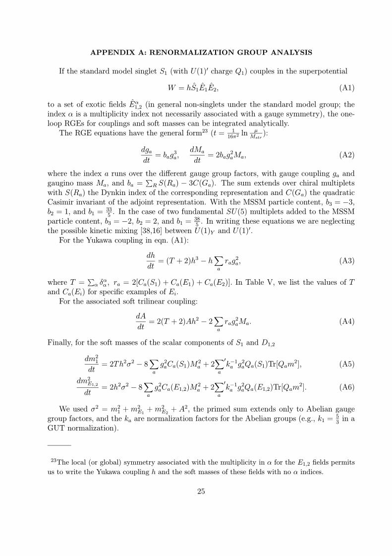
second model.The RGEs of the models (16)-(18) are presented in a general form in the Appendix13.

We have solved the RGEs in each case for a range of boundary conditions to determine therange of µRAD. Each of the models considered has the advantage that it is possible to obtainexact analytical solutions to the RGEs, which yield insight into the nature of the dependenceof the parameters on their initial values. Exact solutions [19] are possible in these modelsbecause the RGEs for the Yukawa couplings are decoupled. In more complicated cases, e.g.,if the same singlet couples to both triplets and doublets, no simple exact solutions exist. Itis also useful to consider simpler semi-analytic solutions to the RGEs, in which the runningof the gauge couplings and gaugino masses is neglected in the solutions of the RGEs of theother parameters. The exact and semi-analytic solutions are presented in Appendix A. Theresults of the renormalization group analysis are presented in Tables I-III for Models (I)-(III),respectively. The evolution of the parameters of Model (I) is shown in some representativegraphs.

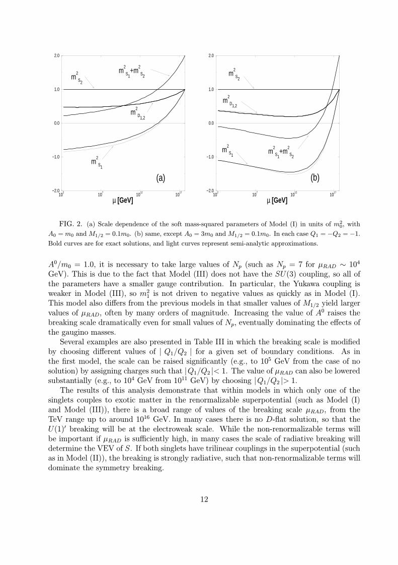
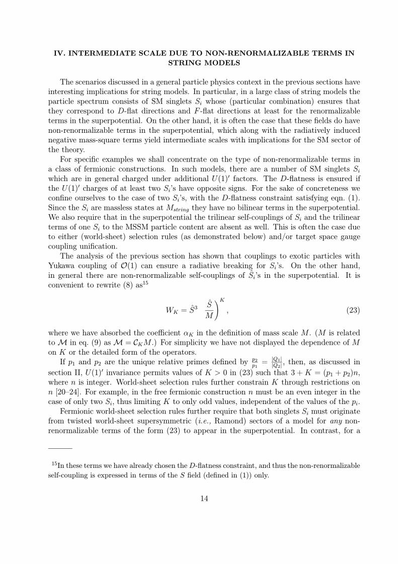
Model (I): In Table I, we present the results of the analysis of Model (I). We first choosethe U(1)′ charge assignment Q1 = −Q2 = −1 for the singlets S1 and S2 and investigate thenature of µRAD as a function of the initial values of the dimensionless ratios A0/m0 andM1/2/m0. The scale dependence of the Yukawa coupling14 and the trilinear coupling areshown in Figure 1. With this choice of U(1)′ charges and A0 = m0, the breaking scale isof the order 1010 GeV for values of M1/2 = O(m0). However, radiative breaking (along theD-flat direction) is not achieved for small values of the initial gaugino masses, as is alsoshown in Figure 2 (a). The gaugino mass parameter M1/2 governs the fixed point behaviorof the soft mass-squared parameters (as was also found in [10]), such that small gauginomasses do not drive m2

1 sufficiently negative to overcome the fact that m22 does not run

significantly because it does not have any couplings in the superpotential. S1 will acquirean electroweak scale VEV in this case, as was described in Section I. Increasing the valueof A0 increases µRAD dramatically (up to 1017 GeV), for it drives m2

1 negative at a higherscale; this behavior is also shown for the case of A0/m0 = 3.0, M1/2/m0 = 0.1 in Figure2 (b). The breaking scale decreases significantly (in some cases, all the way to the TeVrange) when both A0/m0 and M1/2/m0 are lowered simultaneously. This is to be expected,for this is equivalent to raising the initial value of the soft mass-squared parameters andkeeping A0 = M1/2, in which case m2

1 is driven negative at a lower scale.For a given set of boundary conditions, it is also possible to raise or lower µRAD by

choosing different values of the ratio of |Q1/Q2 |, as can be seen from (5). In particular,

13The running of the U(1)′ gauge coupling depends on the charge assignments of all of the fields

in the theory, and so is highly model dependent. For simplicity, we assume that the U(1)′ charge

assignments are such that the evolution of g′1 is identical to that of g1.

14The evolution of the Yukawa coupling for large initial values demonstrates the fixed point

behavior, as discussed in the Appendix.

10

102

107

1012

1017

µ [GeV]0.0

0.5

1.0

1.5

2.0

h

(a)

102

107

1012

1017

µ [GeV]0.0

0.2

0.4

0.6

0.8

1.0

A

(b)

FIG. 1. (a) Scale dependence of the Yukawa coupling of Model (I) for h0 = g0

√2 and h0 = 10. (b)

Scale dependence of the trilinear coupling of Model (I) in units of m0, with M1/2 = 0.1m0. In each case

Q1 = −Q2 = −1. Bold curves are for exact solutions, and light curves represent semi-analytic approxima-

tions.

|Q1/Q2 |> 1 will increase the relative weight of m22 and so decrease µRAD, while |Q1/Q2 |< 1

will increase the relative weight of m21 and thus increase µRAD. Several examples of this type

are presented in Table I. The values of µRAD for the examples with M1/2/m0 = 1.0 shouldbe contrasted with the value of 1010 GeV obtained with Q1 = −Q2 = −1, and the valueswith M1/2/m0 = 0.1 should be compared with the result that radiative breaking does notoccur in the case with equal and opposite U(1)′ charges.

Model (II): The results of the analysis of Model (II) are presented in Table II. Inthis case, both m2

1 and m22 are driven negative due to the large Yukawa couplings in the

superpotential. Thus, µRAD is generally much higher than in the case of the model previouslydiscussed, of order 1013 to 1017 GeV for Q1 = −Q2 = −1. The breaking scale increaseswith larger values of M1/2 and A0, and the effects of the gaugino masses are negligible forsufficiently large values of A0/m0. The breaking scale can be lowered to the range of 1011

GeV by decreasing the values of A0/m0 and M1/2/m0. In this model, changing the value of|Q1/Q2 | does not have a significant effect on µRAD, as the soft mass-squared parameters ofboth singlets are driven to negative values.

Model (III): In Table III, we present the results of the analysis of Model (III), in whichS1 couples to identical pairs of singlets charged under the U(1)′, and S2 has no couplings inthe renormalizable superpotential. In this case, the number of pairs of singlets is analogousto the group theoretical weight in the RGEs, such that m2

1 is driven negative at some scale.While Np = 3 gives the same weight as that of the first model with exotic triplets, the valuesof µRAD shown in the first two entries of Table III demonstrate that this model does notmimic the first model. For example, the results show that to obtain radiative breaking for

11

102

107

1012

1017

µ [GeV]−2.0

−1.0

0.0

1.0

2.0

m2

S2

m2

D1,2

m2

S1

m2

S1+m

2

S2

(a)

102

107

1012

1017

µ [GeV]−2.0

−1.0

0.0

1.0

2.0

m2

S1+m

2

S2m

2

S1

m2

D1,2

m2

S2

(b)

FIG. 2. (a) Scale dependence of the soft mass-squared parameters of Model (I) in units of m20, with

A0 = m0 and M1/2 = 0.1m0. (b) same, except A0 = 3m0 and M1/2 = 0.1m0. In each case Q1 = −Q2 = −1.

Bold curves are for exact solutions, and light curves represent semi-analytic approximations.

A0/m0 = 1.0, it is necessary to take large values of Np (such as Np = 7 for µRAD ∼ 104

GeV). This is due to the fact that Model (III) does not have the SU(3) coupling, so all ofthe parameters have a smaller gauge contribution. In particular, the Yukawa coupling isweaker in Model (III), so m2

1 is not driven to negative values as quickly as in Model (I).This model also differs from the previous models in that smaller values of M1/2 yield largervalues of µRAD, often by many orders of magnitude. Increasing the value of A0 raises thebreaking scale dramatically even for small values of Np, eventually dominating the effects ofthe gaugino masses.

Several examples are also presented in Table III in which the breaking scale is modifiedby choosing different values of | Q1/Q2 | for a given set of boundary conditions. As inthe first model, the scale can be raised significantly (e.g., to 105 GeV from the case of nosolution) by assigning charges such that |Q1/Q2 |< 1. The value of µRAD can also be loweredsubstantially (e.g., to 104 GeV from 1011 GeV) by choosing |Q1/Q2 |> 1.

The results of this analysis demonstrate that within models in which only one of thesinglets couples to exotic matter in the renormalizable superpotential (such as Model (I)and Model (III)), there is a broad range of values of the breaking scale µRAD, from theTeV range up to around 1016 GeV. In many cases there is no D-flat solution, so that theU(1)′ breaking will be at the electroweak scale. While the non-renormalizable terms willbe important if µRAD is sufficiently high, in many cases the scale of radiative breaking willdetermine the VEV of S. If both singlets have trilinear couplings in the superpotential (suchas in Model (II)), the breaking is strongly radiative, such that non-renormalizable terms willdominate the symmetry breaking.

12

Q1,Q2 A0/m0 M1/2/m0 µRAD(GeV) Q1,Q2 A0/m0 M1/2/m0 µRAD(GeV)

−1,1 1.0 1.0 2.7× 1010 −1,1 0.3 0.3 2.0× 103

−1,1 1.0 0.1 – −54 ,3

4 1.0 1.0 3.3× 108

−1,1 3.0 1.0 1.5× 1015 −54 ,1

3 1.0 1.0 2.1× 104

−1,1 3.0 0.1 1.1× 1015 −1,13 1.0 1.0 2.3× 105

−1,1 5.0 1.0 8.8× 1016 −1,14 1.0 1.0 2.1× 103

−1,1 1.0 0.5 2.6 × 107 −12 ,1 1.0 0.1 6.0× 108

−1,1 0.5 0.5 2.4 × 106 −13 ,1 1.0 0.1 1.5 × 1011

−1,1 0.7 0.7 3.2 × 108 −13 ,1

2 1.0 0.1 2.3× 105

TABLE I. Model (I). Singlet coupled to triplets: W = hD1D2S1.

Q1,Q2 A0D/m0,A0

L/m0 M1/2/m0 µRAD(GeV) Q1,Q2 A0D/m0,A0

L/m0 M1/2/m0 µRAD(GeV)

−1,1 1.0,1.0 1.0 1.0× 1014 −1,1 1.0,3.0 0.1 4.4 × 1015

−1,1 1.0,1.0 0.1 1.1× 1013 −1,1 3.0,3.0 1.0 4.0 × 1016

−1,1 3.0,1.0 1.0 1.1× 1016 −1,1 5.0,5.0 1.0 1.9 × 1017

−1,1 3.0,1.0 0.1 1.1× 1016 −1,1 0.3,0.3 0.3 1.9 × 1012

−1,1 1.0,3.0 1.0 4.4× 1015 −1,1 0.1,0.1 0.1 7.4 × 1011

TABLE II. Model (II). Singlets coupled to triplets and doublets: W = hDD1D2S1 + hLL1L2S2.

Q1,Q2,Np A0/m0 M1/2/m0 µRAD(GeV) Q1,Q2,Np A0/m0 M1/2/m0 µRAD(GeV)

−1,1,3 1.0 1.0 – −1,1,8 1.5 0.1 3.9 × 1011

−1,1,3 1.0 0.1 – −1,1,10 1.5 1.0 8.7 × 1011

−1,1,7 1.0 1.0 – −1,1,3 3.0 1.0 7.9 × 1012

−1,1,7 1.0 0.1 3.4× 104 −1,1,3 3.0 0.1 3.8 × 1013

−1,1,8 1.0 1.0 – −1,1,4 3.0 1.0 4.8 × 1014

−1,1,8 1.0 0.1 3.5× 107 −1,1,4 3.0 0.1 4.2 × 1015

−1,1,10 1.0 1.0 1.4× 107 −13 ,1,3 1.0 0.1 6.4× 104

−1,1,10 1.0 0.1 1.1 × 1010 −12 ,1,3 1.5 0.1 1.0× 105

−1,1,3 1.5 1.0 – −1, 45 ,8 1.5 0.1 4.4× 104

−1,1,8 1.5 1.0 3.2× 108 −1, 23 ,4 3.0 0.1 3.6 × 1012

TABLE III. Model (III). Singlet coupled to singlet pairs: W = h∑Npi=1 SaiSbiS1.

13

IV. INTERMEDIATE SCALE DUE TO NON-RENORMALIZABLE TERMS IN

STRING MODELS

The scenarios discussed in a general particle physics context in the previous sections haveinteresting implications for string models. In particular, in a large class of string models theparticle spectrum consists of SM singlets Si whose (particular combination) ensures thatthey correspond to D-flat directions and F -flat directions at least for the renormalizableterms in the superpotential. On the other hand, it is often the case that these fields do havenon-renormalizable terms in the superpotential, which along with the radiatively inducednegative mass-square terms yield intermediate scales with implications for the SM sector ofthe theory.

For specific examples we shall concentrate on the type of non-renormalizable terms ina class of fermionic constructions. In such models, there are a number of SM singlets Siwhich are in general charged under additional U(1)′ factors. The D-flatness is ensured ifthe U(1)′ charges of at least two Si’s have opposite signs. For the sake of concreteness weconfine ourselves to the case of two Si’s, with the D-flatness constraint satisfying eqn. (1).Since the Si are massless states at Mstring they have no bilinear terms in the superpotential.We also require that in the superpotential the trilinear self-couplings of Si and the trilinearterms of one Si to the MSSM particle content are absent as well. This is often the case dueto either (world-sheet) selection rules (as demonstrated below) and/or target space gaugecoupling unification.

The analysis of the previous section has shown that couplings to exotic particles withYukawa coupling of O(1) can ensure a radiative breaking for Si’s. On the other hand,in general there are non-renormalizable self-couplings of Si’s in the superpotential. It isconvenient to rewrite (8) as15

WK = S3

(S

M

)K, (23)

where we have absorbed the coefficient αK in the definition of mass scale M . (M is relatedto M in eq. (9) asM = CKM .) For simplicity we have not displayed the dependence of Mon K or the detailed form of the operators.

If p1 and p2 are the unique relative primes defined by p2

p1= |Q1||Q2|

, then, as discussed in

section II, U(1)′ invariance permits values of K > 0 in (23) such that 3 + K = (p1 + p2)n,where n is integer. World-sheet selection rules further constrain K through restrictions onn [20–24]. For example, in the free fermionic construction n must be an even integer in thecase of only two Si, thus limiting K to only odd values, independent of the values of the pi.

Fermionic world-sheet selection rules further require that both singlets Si must originatefrom twisted world-sheet supersymmetric (i.e., Ramond) sectors of a model for any non-renormalizable terms of the form (23) to appear in the superpotential. In contrast, for a

15In these terms we have already chosen the D-flatness constraint, and thus the non-renormalizable

self-coupling is expressed in terms of the S field (defined in (1)) only.

14

renormalizable trilinear self-coupling S3 term to appear, one of the two Si must have itsorigin in the untwisted Neveu-Schwarz sector while the other comes from a Ramond sector[22,23]. Thus, renormalizable (K = 0) and non-renormalizable (K > 0) terms of the form(23) are mutually exclusive.

The coefficients of the non-renormalizable couplings can be calculated in a large class ofstring models. For the free fermionic construction, coefficient values can be cast in terms ofthe K + 3–point string amplitude, AK+3, in the the following form:16

(1

M

)K≡(αKMP l

)K, (24)

= (2α′)K/2

AK+3 (25)

= (2α′)K/2

(g

2π

)KgηCKIK (26)

= M−KPl

(4√π

)KgηCKIK (27)

(28)

where g is the gauge coupling at Mstring, η =√

2 is a normalization factor (defined so thatthe three-gauge-boson and two-fermion–one-gauge-boson couplings are simply g), 2α′ ≡(64π)/(M2

P lg2) is the string tension [1], CK is the coefficient of O(1) that encompasses

different renormalization factors in the operator product expansion (OPE) of the stringvertex operators (including the target space gauge group Clebsch-Gordon coefficients), andαK ≡ (4/

√π)KgηCKIK . IK is the world-sheet integral of the type:

IK =∫d2z3 · · · d

2zK+2fK(z1 =∞, z2 = 1, z3, · · · , zK+2, zK+3 = 0), (29)

where zi is the world-sheet coordinate of the vertex operator of the ith string state. Asa function of the world-sheet coordinates, fK is a product of correlation functions formedrespectively from the spacetime kinematics, Lorentz symmetry, ghost charge, local non-Abelian symmetries, local and global U(1) symmetries, and (non)-chiral Ising model factorsin each of the vertex operators for the 3 + K fields. All correlators but the Lorentz andIsing ones are of exponential form. For non-Abelian symmetries and for U(1) symmetriesand ghost systems these exponential correlators have the respective generic forms

〈∏i

ei~Qi· ~J〉 =

∏i<j

z~Qi· ~Qjij and 〈

∏i

eiQiH〉 =∏i<j

zQiQjij (30)

where zij = zi − zj . In this language, Qi is imaginary for ghost systems.While the Lorentz correlator is non-exponential, it is nevertheless trivial and contributes

a simple factor of z−1/212 to fK . On the other hand, the various Ising correlators are gener-

ically non-trivial. This makes IK difficult to compute. In fact, Ising correlators generally

16For the explicit calculation of the non-renormalizable terms in a class of fermionic models, see

[23,25].

15

prevent a closed form expression for an integral IK [23]. Nevertheless, Ising fermions maybe necessary in fermionic models for obtaining realistic gauge groups and (quasi)-realisticphenomenology [23,7]. Thus, although the Ising correlation functions make IK increasinglydifficult to compute as K grows in value, Ising correlation functions generally enter stringamplitudes.

From [23,25] we infer that I1 ∼ 70 and I2 ∼ 400. In [23,25], the non-renormalizableterms for which I1 and I2 were calculated involved only one and two MSSM singlets, re-spectively. However, we do not expect that the values of Isinglets1 or Isinglets2 associated withterms composed totally of S-type singlets will generically vary significantly from the valuesobtained when some non-singlets are involved.

For a K = 1 term composed solely of non-Abelian singlets17 carrying U(1)′ charge [6],we have explicitly calculated a value for Isinglets1 . For comparative purposes we relate ourIsinglets1 to the associated four-point string amplitude Asinglets4 via the normalization,

Asinglets4 =g

2π

1

4Isinglets1 . (31)

This is the same normalization as in [25], where the value of I1 was 77.7. The four singletcase produces

Isinglets1 = 2√

2∫d2z |z|−1|1− z|−3/2. (32)

By shifting z → z + 1 and converting the world-sheet coordinate z to polar coordinates(r, θ), the integral can be expressed as

Isinglets1 = 4√

2∫ ∞

0dr∫ π

0dθ

1

1 + r2 − 2r cos θ. (33)

Integrating over the angle θ results in

Isinglets1 = 4√

2∫ ∞

0dr

1

r

2√r

r + 1K

(2√r

r + 1

)(34)

= 8√

2∫ ∞

0dl

2

l2 + 1K

(2l

l2 + 1

), (35)

where K is the complete elliptic integral of the first kind.Numerical approximation of (33) (after splitting integration over r into two separate

regions 0 ≤ r ≤ 1 and 0 ≤ r ≤ ∞) via Mathematica yields a value of Isinglets = 63.7. As a

test of the numerical approximation, we can also expand K in powers of 2√r

r+1(or in powers

of 2ll2+1

) and then integrate the first two (or more) terms in this series. This latter approach

yields (for two terms) Isinglets1 ≈ (9/√

2)π2 ≈ 62.8±10%, in excellent agreement with the our

17The four states forming this K = 1 superpotential term were denoted H30, H32, H37, and H39

in Table 2 of [6]. The first two of these states originate in one sector of the model, while the latter

two reside in a second sector. This is the general pattern also followed in [23,25].

16

numerical approximation.18 Thus the non-singlet factor in the four-point string amplitudeof [25] causes I1 to be about 20% larger than Isinglets1 .

It is expected that the interference terms in IK are generically such that IK < IK1 , andthus M > M1. In particular, for K = 1 we obtain: M1 ∼ 3× 1017 GeV using I1 ∼ 70 andfor K = 2: M2 ∼ 7× 1017 GeV using I2 ∼ 400.

V. NON-RENORMALIZABLE COUPLING TO THE MSSM PARTICLES

The flat direction S can have a set of non-renormalizable couplings to MSSM states thatoffer solutions to the µ problem [26] and yield mass hierarchies between generations [28].The non-renormalizable µ-generating terms are of the form,

Wµ ∼ H1H2S

(S

M

)P. (37)

In addition, the effective soft SUSY-breaking B-term, BH1H2 + H.c. in the Higgs potential,which is necessary for a correct electroweak symmetry breaking, can appear via mixed F -terms from a superpotential19

WB ∼ H1H2S

(S

M

)P+ S3

(S

M

)K, (38)

or from supersymmetry breaking terms [27] in the potential of the type

V ∼ AH1H2S(S

M

)P+ H.c., (39)

where A ∼ msoft. In both cases, when the effective µ parameter is of the order of theelectroweak scale, B ∼ m2

soft automatically.Generational up, down, and electron mass terms appear, respectively, via

Wui ∼ H2QiUci

(S

M

)P ′ui; Wdi ∼ H1QiD

ci

(S

M

)P ′di

; Wei ∼ H1LiEci

(S

M

)P ′ei, (40)

18x ≡ 2√r/(r + 1) is within the range of convergence 0 ≤ x < 1 of the series expansion,

K(x) =π

2

{1 + (

1

2)x+ (

1 · 3

2 · 4)2x2 + · · ·

}, (36)

for all values of r except for r = 1. At r = 1, x reaches the endpoint of convergence, x = 1, for

which limx→1K(x)→∞. As consistency between our two estimates of Isinglets1 indicates, inclusion

of this endpoint in the range of integration of the series expansion still permits using the series

expansion.

19Although the values of the M in the two terms of eqn. (38) are expected to be of the same order

of magnitude, they may vary somewhat. For simplicity, we ignore the distinction.

17

with i denoting generation number20.Majorana and Dirac neutrino terms may also be present via,

W(Maj)LiLi

∼

(H2Li

)2

M

(S

M

)P ′′LiLi; W

(Dir)Liν

ci∼ H2Liν

ci

(S

M

)P ′Liν

ci

;

W(Maj)νci ν

ci∼ νci ν

ci S

(S

M

)Pνciνci

. (41)

(ν ∈ L represents the neutrino doublet component and we have introduced neutrino singletsνc.)

When the VEV 〈S〉 is fixed solely by the running of m2, the size of the µ parameter

will be determined by the scale µRAD and the value of P in eqn. (37), µeff ∼µP+1RAD

MP . Forexample, for P = 1 a reasonable µeff ∼ 1 TeV would correspond to µRAD ∼ 1010 GeV. Onthe other hand, concrete order of magnitude estimates can be made when the VEV is fixedby non-renormalizable self-interactions of S. Generally, if µRAD � 1012 GeV running is thedominant factor; whereas, if µRAD � 1012 GeV the non-renormalizable operators (NRO)

dominate instead. With NRO-dominated 〈S〉 ∼ (msoftMK)

1K+1 , the effective Higgs µ-term

takes the form,

µeff ∼ msoft

(msoft

M

)P−KK+1

. (42)

The phenomenologically preferred choice among such terms is clearly P = K, yielding aK−independent µeff ∼ msoft. Both of these intermediate scale scenarios are to be con-trasted to the case in which 〈S〉 is at the electroweak scale. Then, µeff ∼ msoft can begenerated by a renormalizable (P = 0) term [10].

Quark and lepton masses can have hierarchical patterns generated through

mui ∼ 〈H2〉(msoft

M

) P′ui

K+1

; mdi ∼ 〈H1〉(msoft

M

) P′

diK+1

; mei ∼ 〈H1〉(msoft

M

) P′ei

K+1

. (43)

In (43) we ignore the running of the effective Yukawas below 〈S〉 (or below MP l for mt)because such effects are small compared to the uncertainties in M .

Comparison of the physical fermion mass ratios [33] in Table IV with theoretical K andP dependent mass values in Table V suggests that the set

P′

1 ≡ P′

u1= P

′

d1= P

′

e1= 2;

P′

2 ≡ P′

u2= P

′

d2= P

′

e2= 1; (44)

20Alternatively, non-renormalizable chiral supermultiplet mass terms can be generated through

anomalous U(1)′ breaking [29,30]. Typically, in that case the analogue of 〈s〉/M ∼ 1/10, so that

larger values of P ′ are required.

18

mu : mc : mt = 3× 10−5 : 7× 10−3 : 1

md : ms : mb = 6× 10−5 : 1× 10−3 : 3× 10−2

me : mµ : mτ = 0.3× 10−5 : 0.6 × 10−3 : 1× 10−2

mνe : mνµ : mντ = < 6× 10−11 : < 1× 10−6 : < 1× 10−4

TABLE IV. Fermion mass ratios with the top quark mass normalized to 1. The values of u−,

d−, and s-quark masses used in the ratios (with the t-quark mass normalized to 1 from an assumed

mass of 170 GeV) are estimates of the MS scheme current-quark masses at a scale µ ≈ 1 GeV. The

c- and b-quark masses are pole masses. An additional mass constraint for stable light neutrinos is∑imνi ≤ 6 × 10−11 (i.e., 10 eV), based on the neutrino contributions to the mass density of the

universe and the growth of structure [34].

when used in tandem with K = 5 or K = 6, could produce a fairly realistic hierarchy forthe first two generations in the tanβ ≡ 〈H2〉

〈H1〉∼ 1 limit21. Alternatively, taking the tanβ ∼ 50

limit would suggest slightly higher values for K (while keeping the same set of P ′ values).Presumably mt is associated with a renormalizable coupling (P ′u3

= 0). The other thirdfamily masses do not fit quite as well: they are too small to be associated with renormalizablecouplings, but somewhat larger than is expected for P ′d3

= P ′e3 = 1 for K = 5 or K = 6.However, given the roughness of the estimates and the simplicity of the model, the overallpattern of the masses is quite encouraging. It is also possible that mb and mτ are associatedwith some other mechanism, such as non-renormalizable operators involving the VEV of anentirely different singlet.

There is an obvious constraint on a string model that could produce a generational masshierarchy along these lines, containing P ′1 − 1 = P ′2 = P ′u3

+ 1 = 1 fermion mass terms, intandem with a P = K = 5 or 6 µ-term. A combination of world-sheet selection rules andU(1)′ charges must prevent µ-generating terms with P < 5 from appearing, while allowingthe low order P ′i fermion mass terms. If U(1)′ charges could be assigned by fiat to eachstate, then the U(1)′ symmetry should be able to accomplish this by itself. However, U(1)′

charge assignments are related to modular invariance and thus they cannot be freely chosenfor many states. World-sheet selection rules must likely play a role in constraining P .

The neutrino mass terms in (41) offer various possibilities22 for achieving small neutrinomasses [34], some not involving a traditional seesaw mechanism [35]. Very light non-seesaw

21In Table V we have used the computed value of M1 ∼ 3× 1017 GeV as the value for all M . To

test the validity of this approximation, we have also determinedmQ,L〈Hi〉

andµeffmsoft

for K = 2 using

M2 ∼ 7 × 1017 GeV and for K = 3 using an extrapolated M3 value of 11 × 1017 GeV. For P < 5

and P ′ < K + 5, the better estimates of M2 and M3 reducemQ,L〈Hi〉

andµeffmsoft

, respectively, only by

factors of O(1) in comparison to the values ofmQ,L〈Hi〉

(µeffmsoft

) given in the K = 2- and K = 3-columns

of Table V. However, larger values of P and P ′ yield increasing significant reductions inmQ,L〈Hi〉

andµeffmsoft

, respectively, when the better estimates of M2 and M3 are used.

22Other applications of non-renormalizable operators to neutrino mass include [36] and [37].

19

P or P ′ K = 1 K = 2 K = 3 K = 4 K = 5 K = 6 K = 7(msoftM

) 1K+1 2× 10−8 7× 10−6 1× 10−4 8× 10−4 3× 10−3 6× 10−3 1× 10−2

〈S〉 (GeV) 5× 109 2× 1012 4× 1013 2× 1014 8× 1014 2× 1015 3× 1015

K − 1 5× 107 1× 105 7× 103 1× 103 400 200 90µeffmsoft

K 1 1 1 1 1 1 1

K + 1 2× 10−8 7× 10−6 1× 10−4 8× 10−4 3× 10−3 6× 10−3 1× 10−2

0 1 1 1 1 1 1 1

1 2× 10−8 7× 10−6 1× 10−4 8× 10−4 3× 10−3 6× 10−3 1× 10−2

2 3× 10−16 5× 10−11 2× 10−8 6× 10−7 7× 10−6 4× 10−5 1× 10−4

mQ,L〈Hi〉

3 6× 10−24 3× 10−16 2× 10−12 5× 10−10 2× 10−8 2× 10−7 2× 10−6

4 1× 10−31 2× 10−21 3× 10−16 4× 10−13 5× 10−11 1× 10−9 2× 10−8

5 2× 10−39 2× 10−26 5× 10−20 3× 10−16 1× 10−13 9× 10−12 2× 10−10

TABLE V. Non-Renormalizable MSSM mass terms via 〈S〉. For msoft ∼ 100 GeV,

M ∼ 3× 1017 GeV.

doublet neutrino Majorana masses are possible via W(Maj)LiLi

of the form,

mLiLi ∼〈H2〉2

M

(msoft

M

)P′′

LiLiK+1

∼ 〈H2〉(msoft

M

)×(msoft

M

)P′′

LiLiK+1

� 1 eV (45)

The upper bound on neutrino masses from this term (i.e., the case of P′′

LiLi= 0) is around

10−4 eV (using 〈H2〉 ∼ msoft = 100 GeV and M = 3× 1017 GeV), which is too small to berelevant to dark matter or MSW conversions in the sun [34].

If W(Maj)LiLi

is not present, a superpotential term like W(Dir)Liν

ci

can naturally yield heavierphysical Dirac neutrino masses of the form

mLiνci∼ 〈H2〉

(msoft

M

)P ′Liν

ci

K+1

. (46)

For example, for K = 5 the experimental neutrino upper mass limits given in Table IV allowP ′L1νc1

≥ 4, P ′L2νc2≥ 3, and P ′L3νc3

≥ 2. Masses corresponding to P ′Liνci = 4 or 5 (mLiνci

= 0.9

eV or 10−2 eV, respectively) are in the range interesting for solar and atmospheric neutrinos,oscillation experiments, and dark matter.

Neutrino singlets can acquire a Majorana mass through W(Maj)νci

,

mνci νci∼ msoft

(msoft

M

) Pνciνci−K

K+1

, (47)

which can be very large or small, depending on the sign of Pνci νci − K. Laboratory andcosmological constraints depend on the νci lifetimes (if it decays), cosmological productionand annihilation rates, and mixings with each other and with doublet neutrinos. These inturn depend on other couplings, such as W

(Dir)Liν

ci

or renormalizable couplings not associated

20

with the mass. Generally, however, the constraints are very weak due to the absence ofnormal weak interactions, especially for heavy νci (Pνci νci ≤ K).

If bothW(Dir)Liν

ci

and W(Maj)νci ν

ci

terms are present, the standard seesaw mechanism can produce

light neutrinos via diagonalization of the mass matrix for eqs. (46,47). The light masseigenstate is

mlightseesaw ∼ m2

Liνci/mνci ν

ci∼ msoft

(msoft

M

) 2P ′Liν

ci

+K−Pνciνci

K+1

, (48)

while the heavy mass eigenstate is to first order mνci νci

as given by (47). Various combinationsof K, P ′Liνci and Pνci νci produce viable masses for three generations of light neutrinos. For

example, with K = 5 and P ′Liνci = P ′i = {2, 1} for i = 1, 2, respectively (the values of

K and P ′i=1,2 discussed above for the quarks and electrons), and with either P ′L3νc3= 1 or

P ′L3νc= P ′u3

= 0 (involving a renormalizable Dirac neutrino term), the light eigenvaluesof the three generations fall into the hierarchy of 3 × 10−5 eV, 1 × 10−2 eV, and either1× 10−2 eV or 5 eV for Pνci νci = P ′Liνci + 1. This range is again of interest for laboratory andnon-accelerator experiments.

VI. CONCLUSIONS

We have explored the nature of intermediate scale scenarios for effective supergravitymodels as derived within a class of string vacua. In particular, we explored a class of stringmodels which, along with the SM gauge group and the MSSM particle content, containmassless SM singlet(s) Si. In addition, we assumed that the effects of supersymmetrybreaking are parameterized by soft mass parameters.

The necessary condition for the intermediate mass scenario is the existence of D-flatand F -flat directions in the renormalizable part of the Si sector. In this case, the onlyrenormalizable terms of the potential are due to the soft mass-square parameters m2

i . Ifthe running of the soft mass parameters is such that the effective mass-square, along theflat direction, becomes negative at µRAD � MZ , the Si’s acquire a non-zero VEV at anintermediate scale. (Another possibility is that individual mass squares, but not the effectivecombination for the D-flat direction, are negative. Then the VEV is of the order of theelectroweak scale.)

Importantly, in a large number of string models, in particular for a class of fermionicconstructions, there exist SM singlets Si with flat directions at the renormalizable level,which couple to additional exotic particles via Yukawa couplings of O(1). Such Yukawacouplings in turn ensure the radiative breaking, by driving the soft m2

i parameters negativeat µRAD �MZ .

For simplicity we confined the concrete analysis to the case in which there is an additionalU(1)′ symmetry, and two SM singlets S1,2 have opposite signs of the U(1)′ charges, thusensuring D-flatness for |Q1||S1|2 = |Q2||S2|2 (similar results are expected for the case of asingle standard model singlet and no additional U(1)′). In the analysis of radiative breakingwe considered three types of Yukawa couplings (of O(1)) of Si to the exotic particles and a

21

range of the boundary conditions on soft mass parameters at Mstring. For a large range ofparameters we obtained µRAD in the range 105 GeV to 1016 GeV (or at µRAD ∼MZ).

In addition, we discussed the competition between the effects of the pure radiative break-ing (〈S〉 ∼ µRAD) and the stabilization of vacuum due to the non-renormalizable terms in the

superpotential of the type SK+3/MK (〈S〉 ∼ (msoftMK)1

K+1 ). Non-renormalizable termsin the superpotential are generic (and calculable) in string models. For a class of fermionic

constructions M ∼Mstring. These terms are dominant for (msoftMK)1

K+1 < µRAD.In the case of the pure radiative breaking, the mass of the Higgs field (and its fermionic

partner) associated with non-zero VEV of S is light and of order MZ/(4π). On the otherhand, the breaking due to the non-renormalizable terms implies a light Higgs field and thesupersymmetric partner both with the mass of order MZ .

The non-renormalizable couplings of Si’s to the MSSM particles in the superpotential inturn provide a mechanism to obtain an effective µ parameter and the masses for quarks andleptons. In the case of the pure radiative breaking the precise values of the µ parameter andthe lepton-quark masses crucially depends on µRAD. When the non-renormalizable termsdominate, these parameters assume specific values in terms of K and the order P of the non-renormalizable term by which they are induced. In particular, µ = O(msoft) for K = P , thusproviding a phenomenologically acceptable value for the µ parameter. (Another possibilityis that in which the U(1)′ is broken at the electroweak scale and the effective µ is generatedby a renormalizable term.) We are able to obtain interesting hierarchies for the quark andlepton masses for appropriate values of P . Also, small (non-seesaw) Dirac or Majorananeutrino masses can be obtained, or the traditional seesaw mechanism can be incorporated,depending on the nature of the non-renormalizable operators.

In conclusion, the string models provide an important framework in which the interme-diate scales can naturally occur and provide interesting implications for the µ parameterand the fermion mass hierarchy of the MSSM sector.

ACKNOWLEDGMENTS

This work was supported in part by U.S. Department of Energy Grant No. DOE-EY-76-02-3071. We thank P. Steinhardt and I. Zlatev for useful discussions.

22

REFERENCES

[1] V. Kaplunovsky, Nucl. Phys. B307, 145 (1988), [E-B383, 436 (1992)].[2] L. Dixon, J. A. Harvey, C. Vafa and E. Witten, Nucl. Phys. B261, 678 (1985); B274,

285 (1986).[3] A. Font, L. E. Ibanez, F. Quevedo and A. Sierra, Nucl. Phys. B331, 421 (1991).[4] I. Antoniadis, C. Bachas and C. Kounnas, Nucl. Phys. B289, 87 (1987); H. Kawai, D.

Lewellen and S.H.-H. Tye, Phys. Rev. Lett. 57, 1832 (1986); Phys. Rev. D34, 3794(1986).

[5] I. Antoniadis, J. Ellis, J. Hagelin and D. Nanopoulos, Phys. Lett. B231, 65 (1989).[6] A. Faraggi, D.V. Nanopoulos and K. Yuan, Nucl. Phys. B335, 347 (1990); A. Faraggi,

Phys. Lett. B278, 131 (1992).[7] S. Chaudhuri, S.-W. Chung, G. Hockney and J. Lykken, Nucl. Phys. B456, 89 (1995);

S. Chaudhuri, G. Hockney and J. Lykken, Nucl. Phys. B469, 357 (1996).[8] K.R. Dienes, [hep-th/9602045].[9] M. Cvetic and P. Langacker, Phys. Rev. D54, 3570 (1996), and Mod. Phys. Lett. 11A,

1247 (1996).[10] M. Cvetic, D.A. Demir, J.R. Espinosa, L. Everett and P. Langacker, Phys. Rev. D56,

2861 (1997).[11] D. Suematsu and Y. Yamagishi, Int. J. Mod. Phys. A10, 4521 (1995); E. Keith and E.

Ma, preprint UCRHEP-T-176 [hep-ph/9704441].[12] J.A. Adams, G.G. Ross and S. Sarkar, Oxford preprint OUTP-96-58P [hep-ph/9704286].[13] See K.R. Dienes and A. Faraggi, Nucl. Phys. B457, 409 (1995), and references therein;

P. Binetruy and P. Langacker, in preparation.[14] M. Dine, V. Kaplunovsky, M. Mangano, C. Nappi and N. Seiberg, Nucl. Phys. B259,

549 (1985); G. Costa, F. Feruglio, F. Gabbiani and F. Zwirner, Nucl. Phys. B286, 325(1987); J. Ellis, K. Enqvist, D.V. Nanopoulos and K. Olive, Phys. Lett. 188B, 415(1987); R. Arnowit and P. Nath, Phys. Rev. Lett. 60, 1817 (1988).

[15] L. Ibanez, CERN-TH-5157/88, Strings ’88; Y. Kawamura and T. Kobayashi, Nucl.Phys. B481 539 (1996).

[16] K. Dienes, C. Kolda and J. March-Russell, Nucl. Phys. B492 104 (1997).[17] B. de Carlos, J.A. Casas and C. Munoz, Phys. Lett. B299, 234 (1993); A. Brignole,

L. Ibanez and C. Munoz, Nucl. Phys. B422, 125 (1994).[18] M. Drees, Phys. Lett. B181, 279 (1986); H.-C. Cheng and L. Hall, Phys. Rev. D51, 1337

(1995); C. Kolda and S. Martin, Phys. Rev. D53, 3871 (1996); J.D. Lykken, preprintFERMILAB-CONF-96/344-T, [hep-ph/9610218].

[19] L. Ibanez and C. Lopez, Nucl. Phys. B233, 511 (1984); L. Ibanez, C. Lopez and C.Munoz, Nucl. Phys. B256, 218 (1985).

[20] M. Cvetic, Phys. Rev. Lett. 59 (1987) 1795; Phys. Rev. D37 (1988) 2366.[21] A. Font, L. E. Ibanez, H.P. Nilles and F. Quevado, Nucl. Phys. B307 109 (1988); Phys.

Lett. B210 101 (1988); Phys. Lett. B213 274 (1988).[22] J. Rizos and K. Tamvakis, Phys. Lett. B262, 227 (1991).[23] S. Kalara, J. Lopez, and D. Nanopoulos, Nucl. Phys. B353, 650 (1991).[24] T. Kobayashi, Phys. Lett. B354, 264 (1995).[25] A. Faraggi, Nucl. Phys. B487, 55 (1997).

23

[26] J.E. Kim and H.P. Nilles, Phys. Lett. B138, 150 (1984).[27] Y. Kawamura, T. Kobayashi, and M. Watanabe, preprint DPSU-97-5 [hep-ph/9705272].[28] T. Kobayashi, Phys. Lett. B358, 253 (1995);[29] A. Faraggi, Nucl. Phys. B403, 101 (1993); Phys. Lett. B274, 47 (1992).[30] P. Ramond, Toyonaka 1995 [hep-ph/9604251]; P. Binetruy, N. Irges, S. Lavignac and

P. Ramond, Phys. Lett. B403, 38 (1997); J.K. Elwood, N. Irges and P. Ramond, [hep-ph/9705270].

[31] A. Faraggi, Nucl. Phys. B387 239 (1992); Nucl. Phys. B407 57 (1993).[32] S. Kalara, J. Lopez, and D.V. Nanopoulos, Phys. Lett. B245 421 (1990); Ibid, Phys.

Lett. B287 82, (1992); J. Lopez and D.V. Nanopoulos, Phys. Lett. B251 73 (1990).[33] R. Barnett et al., Reviews of Particle Properties, Phys. Rev. D54, 1 (1996).[34] For detailed reviews, see G. Gelmini and E. Roulet, Rept. Prog. Phys. 58, 1207 (1995);

P. Langacker in Testing The Standard Model, ed. M. Cvetic and P. Langacker (World,Singapore, 1991) p. 863.

[35] M. Gell-Mann, P. Ramond, and R. Slansky, in Supergravity, ed. F. van Nieuwenhuizenand D. Freedman, (North Holland, Amsterdam, 1979) p. 315; T. Yanagida, Proc. of theWorkshop on Unified Theory and the Baryon Number of the Universe, KEK, Japan,1979; S. Weinberg, Phys. Rev. Lett. 43, 1566 (1979).

[36] E. K. Akhmedov, Z. G. Berezhiani, and G. Senjanovic, Phys. Rev. Lett 69, 3013 (1992),Phys. Rev. D47 3245 (1993).

[37] M. Cvetic and P. Langacker, Phys. Rev. D46, R2759 (1992).[38] F. del Aguila, G.D. Coughlan and M. Quiros; Nucl. Phys. B307, 633 (1988), [E-B312,

751 (1989)]; F. del Aguila, M. Masip and M. Perez-Victoria, Nucl. Phys. B456, 531(1995).

24

APPENDIX A: RENORMALIZATION GROUP ANALYSIS

If the standard model singlet S1 (with U(1)′ charge Q1) couples in the superpotential

W = hS1E1E2, (A1)

to a set of exotic fields Eα1,2 (in general non-singlets under the standard model group; the

index α is a multiplicity index not necessarily associated with a gauge symmetry), the one-loop RGEs for couplings and soft masses can be integrated analytically.

The RGE equations have the general form23 (t = 116π2 ln µ

Mstr):

dga

dt= bag

3a,

dMa

dt= 2bag

2aMa, (A2)

where the index a runs over the different gauge group factors, with gauge coupling ga andgaugino mass Ma, and ba =

∑R S(Ra) − 3C(Ga). The sum extends over chiral multiplets

with S(Ra) the Dynkin index of the corresponding representation and C(Ga) the quadraticCasimir invariant of the adjoint representation. With the MSSM particle content, b3 = −3,b2 = 1, and b1 = 33

5. In the case of two fundamental SU(5) multiplets added to the MSSM

particle content, b3 = −2, b2 = 2, and b1 = 385

. In writing these equations we are neglectingthe possible kinetic mixing [38,16] between U(1)Y and U(1)′.

For the Yukawa coupling in eqn. (A1):

dh

dt= (T + 2)h3 − h

∑a

rag2a, (A3)

where T =∑α δ

αα , ra = 2[Ca(S1) + Ca(E1) + Ca(E2)]. In Table V, we list the values of T

and Ca(Ei) for specific examples of Ei.For the associated soft trilinear coupling:

dA

dt= 2(T + 2)Ah2 − 2

∑a

rag2aMa. (A4)

Finally, for the soft masses of the scalar components of S1 and D1,2

dm21

dt= 2Th2σ2 − 8

∑a

g2aCa(S1)M2

a + 2∑a

′k−1a g2

aQa(S1)Tr[Qam2], (A5)

dm2E1,2

dt= 2h2σ2 − 8

∑a

g2aCa(E1,2)M2

a + 2∑a

′k−1a g2

aQa(E1,2)Tr[Qam2]. (A6)

We used σ2 = m21 + m2

E1+ m2

E2+ A2, the primed sum extends only to Abelian gauge

group factors, and the ka are normalization factors for the Abelian groups (e.g., k1 = 53

in aGUT normalization).

23The local (or global) symmetry associated with the multiplicity in α for the E1,2 fields permits

us to write the Yukawa coupling h and the soft masses of these fields with no α indices.

25

Ei ∼ (SU(3), SU(2), U(1)Y , U(1)′) T C3(Ei) C2(Ei) C1(Ei) C1′(Ei)

D ∼ (3, 0, YD , QD) 3 43 0 3Y 2

D/5 Q2D/k1′

L ∼ (0, 2, YL, QL) 2 0 34 3Y 2

L/5 Q2L/k1′

Si ∼ (0, 0, 0, QSi ) Np 0 0 0 Q2Si/k1′

TABLE VI. Coefficients in RGEs for coupling of S1 to triplets, doublets, and Np pairs of identical

MSSM singlets, via the superpotential W = hS1E1E2. For the numerical work we chose k1′ = 53 .

The solutions for this set of equations24 are:

g2a(t) =

g20

1− 2bag20t, (A7)

Ma(t) = M1/2g2a(t)

g20

, (A8)

h2(t) =E(t)h2

0

1 + (T + 2)h20F (t)

, (A9)

A(t) = A0εf (t) +M1/2

[H2(t)− (T + 2)h2

0H3(t)εf (t)], (A10)

m21(t) = [1− 3TRf(t)]m

20 − TRf(t)εf (t)A2

0 − 2TRf(t)εf (t)H3(t)

F (t)A0M1/2

+ M21/2

I1(t)− TRf(t)J(t)

F (t)+ T (T + 2)

[H3(t)

F (t)

]2

R2f (t)

, (A11)

m2E1,2

(t) = [1− 3Rf (t)]m20 −Rf (t)εf(t)A

20 − 2Rf(t)εf (t)

H3(t)

F (t)A0M1/2

+ M21/2

IE1,2(t)−Rf (t)J(t)

F (t)+ (T + 2)

[H3(t)

F (t)

]2

R2f (t)

, (A12)

where

E(t) =∏a

[1− 2bag20t]

ra/ba , (A13)

F (t) = 2∫ 0

tE(t′)dt′, (A14)

εf(t) =1

1 + (T + 2)h20F (t)

, (A15)

Rf(t) = h20F (t)εf (t), (A16)

H2(t) = −2∑a

rag2a(t)t, (A17)

24Assuming universality of the soft masses at the string scale, Tr[Qam2] = 0 at all scales for

non-anomalous Abelian groups.

26

H3(t) = −2tE(t)− F (t), (A18)

Ik(t) = 2∑a

Ca(k)1

ba

[1−

1

(1− 2bag20t)

2

](A19)

J(t) = 2∫ 0

tE(t′)

[H2

2 (t′) + I1(t′) + IE1(t′) + IE2(t

′)]dt′. (A20)

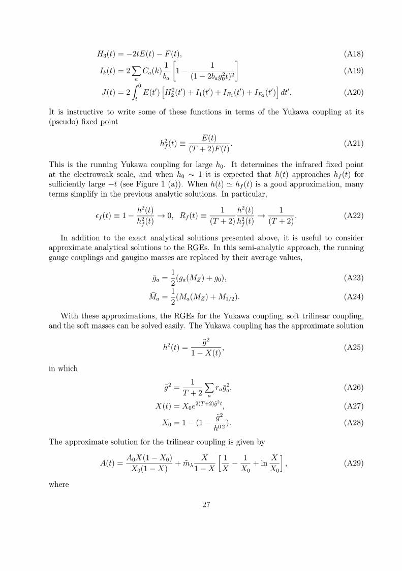
It is instructive to write some of these functions in terms of the Yukawa coupling at its(pseudo) fixed point

h2f(t) ≡

E(t)

(T + 2)F (t). (A21)

This is the running Yukawa coupling for large h0. It determines the infrared fixed pointat the electroweak scale, and when h0 ∼ 1 it is expected that h(t) approaches hf (t) forsufficiently large −t (see Figure 1 (a)). When h(t) ' hf (t) is a good approximation, manyterms simplify in the previous analytic solutions. In particular,

εf(t) ≡ 1−h2(t)

h2f(t)→ 0, Rf (t) ≡

1

(T + 2)

h2(t)

h2f (t)→

1

(T + 2). (A22)

In addition to the exact analytical solutions presented above, it is useful to considerapproximate analytical solutions to the RGEs. In this semi-analytic approach, the runninggauge couplings and gaugino masses are replaced by their average values,

ga =1

2(ga(MZ) + g0), (A23)

Ma =1

2(Ma(MZ) +M1/2). (A24)

With these approximations, the RGEs for the Yukawa coupling, soft trilinear coupling,and the soft masses can be solved easily. The Yukawa coupling has the approximate solution

h2(t) =g2

1−X(t), (A25)

in which

g2 =1

T + 2

∑a

rag2a, (A26)

X(t) = X0e2(T+2)g2t, (A27)

X0 = 1− (1−g2

h0 2). (A28)

The approximate solution for the trilinear coupling is given by

A(t) =A0X(1−X0)

X0(1−X)+ mλ

X

1−X

[1

X−

1

X0+ ln

X

X0

], (A29)

where

27

mλ =1

(T + 2)g2

∑a

rag2aMa, (A30)

and the other quantities are defined above.If the U(1)′ factors are neglected, the soft scalar mass-squared parameters have the

following approximate solutions:

m21 = (1−

T

T + 2)m2

0 +T

T + 2Σ(t) + 2T g2m2 ln

X

X0, (A31)

m2E1,2

= (1−1

T + 2)m2

0 +1

T + 2Σ(t) + (2g2m2 − 8

∑a

Ca(E1,2)M2a g

2a) ln

X

X0, (A32)

in which

m2 =4

(T + 2)g2

∑a

Ca(E1,2)M2a g

2a, (A33)

and

Σ(t) = (m2 − m2λ)

1− XX0

1−X+X(1−X0)

X0(1−X)Σ0 −

X(1−X0)

X0(A0 − mλ)

2 1− XX0

(1−X)2

+X(1−X0)

X0(1−X)2 2(A0 − mλ)mλ lnX

X0+

X

1−XlnX

X0(m2 + m2

λ

1

1−XlnX

X0). (A34)

The semi-analytic solutions are valid in the limit of small initial gaugino masses, such thatthe contribution of the gauginos to the evolution of the trilinear coupling and the soft mass-squared parameters is small.

28