Intermittency and Premixed Turbulent Reacting Flows
Peter E. Hamlington, Alexei Y. Poludnenko, and Elaine S. Oran
Laboratory for Computational Physics and Fluid Dynamics
Naval Research Laboratory, Washington, DC, 20375, USA
Probability density functions (pdfs) of the magnitudes of the vorticity, strain rate, andscalar (reactant mass fraction) gradient are examined in premixed reacting flows usingdirect numerical simulations of stoichiometric hydrogen-air combustion at a range of tur-bulence intensities. Simulations of nonreacting passive scalar evolution in homogeneousisotropic turbulence are also performed in order to validate the numerical method andprovide a baseline against which the reacting flow results can be compared. In the reactingsimulations, conditional analyses based on the local, instantaneous values of the scalar areused to study the variation of the pdfs through the flame, and particular emphasis is placedon the degree of intermittency associated with these pdfs. For small intensities, the pdfsof the vorticity vary substantially through the flame, with stronger intermittency near theproducts. The strain rate pdfs are also intermittent, but undergo less pronounced changesthrough the flame. For high intensities, both the vorticity and strain rate pdfs becomeessentially independent of flame position and remain close to their nonreacting forms. Thescalar gradient intermittency is found to be strongest near the reactants and increases atall flame locations with increased turbulence intensity. For small intensities and in thereaction zone, however, the scalar gradient pdfs approximately follow a Gaussian distribu-tion, resulting in substantially reduced intermittency. Deviations from log-normality areobserved in the pdfs of all quantities, even for intensities and flame locations characterizedby large intermittency.
I. Introduction
Developing a detailed understanding of turbulence-flame interactions in premixed combustion is impor-tant for a number of problems, such as the design of improved spark-ignition and gas turbine engines.1–3
Properties of both the turbulent fluid and the premixed flame in these applications depend on the relativestrength of turbulent and chemical processes at each point in the flow. These processes are nonlinearlycoupled,4 and their interactions vary with both the intensity of the turbulence in the unburned reactantsand location in the flame. The nature of this variation, and the associated changes in the turbulence and theflame, remains a topic of considerable interest in combustion research. Many recent efforts have been aimedat determining the speed and internal structure of turbulent premixed flames, and a number of studies5–8
have begun to investigate these properties in the limit of very intense turbulence.In the present study, we consider turbulence-flame interactions by examining the probability density
functions (pdfs) of the magnitudes of the vorticity, strain rate, and scalar (reactant mass fraction) gradient.Emphasis is placed on understanding the intermittency associated with these pdfs, which can have signifi-cant implications for flame properties.9–11 The analysis is based on direct numerical simulations (DNS) ofstatistically-planar, stoichiometric H2-air premixed flames at a range of turbulence intensities. The intensityis characterized by IT = Urms/SL, where Urms is the rms turbulent velocity in the unburned reactants andSL is the laminar flame speed. Conditional statistics based on the local, instantaneous value of the reactantmass fraction are used to examine the variation of the pdfs through the flame itself. This approach allowsthe pdfs to be studied as a function of both IT and location in the flame.
The present focus on the vorticity, strain rate, and scalar gradient is motivated by the fact that thesequantities provide field representations of both the turbulence and the flame, and allow turbulence-flameinteractions to be quantitatively assessed. The vorticity, ωi, and strain rate, Sij , reflect the small-scale
1 of 13
American Institute of Aeronautics and Astronautics
49th AIAA Aerospace Sciences Meeting including the New Horizons Forum and Aerospace Exposition4 - 7 January 2011, Orlando, Florida
structure of turbulent flows,12 and are given in terms of gradients of the velocity, ui, as
ωi = ǫijk∂uk
∂xj, Sij =
1
2
(
∂ui
∂xj+
∂uj
∂xi
)
, (1)
where ǫijk is the Levi-Civita symbol. Properties of the flame are reflected in the scalar gradient, χi, givenby
χi =∂Y
∂xi, (2)
where Y is the reactant mass fraction. This scalar can be used to parameterize the location in the flame.In the reactants (products), Y = 1 (Y = 0), and for the reaction-diffusion model used here, the Y = 0.6isosurface approximately separates the preheat (Y > 0.6) and reaction (Y < 0.6) zones.7 The direction ofχi in Eq. (2) gives the local flame orientation (its distribution is related to wrinkling of the flame), and themagnitude χ = [χiχi]
1/2 reflects the local flame width.13, 14 Large (small) χ is indicative of a locally thinner(broader) flame.
A prior analysis14 of the first-order statistics – such as conditional averages and relative alignments – ofωi, Sij , and χi has revealed several aspects of the changes in turbulence-flame coupling with IT . It was foundthat for small IT within the reaction zone, ωi and Sij are, on average, suppressed, and χi has propertiessimilar to those of a laminar flame. At small IT within the preheat zone, however, as well as at large ITthroughout the flame, ωi and Sij are only weakly affected by the flame, and the statistics of χi begin toresemble those of a passive scalar gradient. Similar results have also been observed in other studies13, 15–17
of the interactions between χi and Sij .Here we extend these prior analyses and examine the pdfs of the magnitudes ω2 = ωiωi, S
2 = SijSij ,and χ2 = χiχi. These magnitudes are related to the local enstrophy, energy dissipation rate, and scalar dis-sipation, 2Dχ2, where D is the molecular diffusivity. The pdfs of these quantities have received considerableattention in the context of nonreacting turbulent flows (where the scalar is a conserved, passive quantity), butare still not completely understood in premixed reacting flows. In particular, the intermittency associatedwith these pdfs in premixed flames has yet to receive much attention.9, 10 Intermittency is strictly definedas departures from Gaussianity,10, 12, 18, 19 and previous experimental20–22 and computational23–28 studies ofnonreacting turbulence have shown that large magnitudes of ω2, S2, and χ2 occur with substantially higherprobability than predicted by Gaussian statistics. Karpetis and Barlow29 have examined pdfs of 2Dχ2 inpartially-premixed methane-air jet flames, again finding that the pdfs are intermittent.
In reacting flows, intermittency can have a significant effect on fluid properties and flame structure.9
The dissipation rate, 2Dχ2, is connected to the chemical reaction rate,9, 10, 30, 31 and is also used in pdf andconditional moment closure models of turbulent combustion.9, 32 The turbulent vorticity and strain rate fieldsare responsible, in part, for the stretching, wrinkling, and broadening of premixed flames, particularly whenIT is large.14 Large values of ω2 and S2 can thus lead to a substantially altered premixed flame structure.It has also been suggested that turbulence intermittency effects are important in deflagration-to-detonationtransitions, for example in astrophysical explosions involving type Ia supernovae.11
In the following we examine the pdfs and intermittency of ω2, S2, and χ2 using DNS of H2-air premixedcombustion with turbulence intensities IT = 2.45, 9.81, and 30.6. In addition to the reacting flow simula-tions, nonreacting simulations of homogeneous isotropic turbulence with a passive, conserved scalar are alsoexamined. These simulations serve as a validation of the numerical approach and provide a baseline againstwhich the reacting flow results can be compared. In all cases, measured pdfs are compared with log-normaldistributions, which have been studied previously as a potential model for intermittent turbulence.33
II. Numerical Simulations
The numerical simulations represent premixed H2-air combustion in an unconfined domain, and arecarried out using Athena-RFX,7, 8 which is based on the magnetohydrodynamic code Athena.34, 35 Athena-
2 of 13
American Institute of Aeronautics and Astronautics
Table 1. Laminar flame properties and input model parameters common to all numerical simulations.
Simulation (Nonreacting) IT Da τed (s)
F1 (NR1) 2.45 0.387 2.14 × 10⁻⁴
F3 (NR3) 9.81 0.0965 5.36 × 10⁻⁵
F5 (NR5) 30.6 0.0310 1.71 × 10⁻⁵
Table 2. Initial normalized turbulent intensity IT ≡ Urms/SL, Damkohler number, Da = (l/Urms)/(lF /SL), and eddyturnover time, τed = L/UL, in the unburned mixture at ignition for the three reacting simulations, denoted F1, F3, andF5. The corresponding nonreacting simulations with the same IT are denoted NR1, NR3, and NR5.
RFX solves the compressible, inviscid, reactive flow Navier-Stokes equations given by7, 8
∂ρ
∂t+
∂(ρui)
∂xi= 0 , (3)
∂(ρui)
∂t+
∂(ρuiuj)
∂xj+
∂P
∂xi= 0 , (4)
∂E
∂t+
∂[(E + P )uj ]
∂xj−
∂
∂xj
(
K∂T
∂xj
)
= −ρqw , (5)
∂(ρY )
∂t+
∂(ρY uj)
∂xj−
∂
∂xj
(
ρD∂Y
∂xj
)
= ρw , (6)
where ρ is the density, P is the pressure, E is the energy density, T is the temperature, and q is the chemicalenergy release. First-order Arrhenius kinetics7, 8 are used to write the reaction rate w in Eqs. (5) and (6) as
w = −AρY exp
(
−Q
RT
)
, (7)
where A is the pre-exponential factor, Q is the activation energy, and R is the universal gas constant. Thecoefficients of molecular diffusion, D, and thermal conduction, K, are modeled as
D = D0T n
ρ, K = Cpκ0T
n , (8)
where D0, κ0, and n are constants and Cp = γR/M(γ − 1). The ideal gas equation of state is used for P ,and the Lewis number, Le = κ0/D0, is unity for all simulations. The values of the model parameters inEqs. (3)–(8), summarized in Table 1, are based on the reaction model of Gamezo et al.36 and represent astoichiometric H2-air mixture.
A higher-order, fully conservative Godunov-type method35, 37, 38 is used to solve Eqs. (3)–(8). Numericalviscosity is used for energy dissipation, which allows the inertial range to be properly modeled without re-
3 of 13
American Institute of Aeronautics and Astronautics
quiring prohibitively large computational resources.7 A detailed study7, 8 has shown that numerical viscosityallows the properties and dynamics of the turbulent flame to be accurately captured.
Turbulence is sustained in the simulations by introducing isotropic, divergence-free perturbations to thevelocity field at the largest scale of the flow.7 This approach generates fully-developed homogeneous isotropicturbulence with Kolmogorov (k−5/3) scaling in the inertial range of the kinetic energy spectrum.7, 8, 14 Injec-tion of the perturbations is continued even after flame ignition, resulting in sustained interactions betweenthe turbulence and the flame. The time interval between regenerations of the perturbation field is maintainedat τed/200 for all simulations, where τed = L/UL is the eddy-turnover time, L is the physical width of thecomputational domain, and UL is the velocity at scale L.
Three different simulations are examined here, denoted F1, F3, and F5 in Table 2, corresponding toIT = 2.45, 9.81, and 30.6, respectively. These simulations have been studied previously14 as part of aset of five simulations with additional intermediate intensities IT = 4.90 and 18.4 (denoted F2 and F4in Ref. [14]), which are not included in the present analysis. The present simulations are sufficient todetermine trends in the variation of the statistics with IT , and correspond to Damkohler numbers Da ≡(l/Urms)/(lF /SL) = 0.387 − 0.0310, where l is the turbulence integral scale, lF = D(Y = 0.5)/SL ≈ 2δL,δL ≡ (Tb−Tu)/(dT/dx)L,max is the thermal width of the laminar flame, and l/δL = 1.90. The computationaldomain for all simulations has a length-to-width ratio of Lx : (Ly, Lz) = 16 : 1, and the size of the grid isnx × ny × nz = 2048× 128× 128. This gives 16 computational cells per δL, and examination7 of both lower(8 cells per δL) and higher (32 cells per δL) resolutions has shown that the present resolution is sufficient toaccurately capture properties of the flame.
After letting homogeneous isotropic turbulence develop for 2τed, the flame is initialized near the centerof the domain along the x-axis using an exact laminar flame profile. Periodic boundary conditions are usedin the spanwise directions, giving a statistically-planar flame in the y − z plane, with a mean flow in thex-direction. Periodic boundary conditions are used on the x-boundaries prior to the moment of ignition, atwhich time they are switched to zero-order extrapolation boundary conditions to prevent pressure build-upinside the domain. The analysis of the simulations begins 2τed after ignition, and extends for 5τed in eachcase. During the analysis phase, ten snapshots are retained per τed in order to obtain sufficient statisticswhile preserving temporal-independence of the data, giving a total of 50 snapshots in the analysis of eachIT .
In addition to the reacting flow cases, simulations of nonreacting homogeneous isotropic turbulence(with fluid properties identical to those of the unburned reactant mixture) are also carried out. Again threesimulations are performed, denoted NR1, NR3, and NR5 (Table 2), with turbulence intensities correspondingto those used in F1, F3, and F5. The resolution of the nonreacting simulations is the same as that usedfor the reacting cases, with computational dimensions 1283 and periodic boundaries in all directions. Thefluid equations (3)–(6) are solved with D and K again given by Eq. (8) and with w = 0, causing the scalarto be passive and conserved. To avoid confusion with the nonconserved Y in Eq. (6) and χi in Eq. (2),the passive scalar in the nonreacting simulations is denoted ξ and its gradient ζi = ∂ξ/∂xi. The analysisof the nonreacting simulations is carried out for one τed in each case, again with 10 snapshots per τed.Reasonably high statistical convergence is maintained since the entire 1283 spatial domain can be used inthe analysis at each time. This is in contrast to the reacting flow results which must be examined ona conditional basis, resulting in significantly fewer spatial points included in each of the conditional pdfs.Through comparisons with previous experimental studies20 and DNS23–25, 28 of passive scalar evolution, thesenonreacting simulations serve as a validation of the current computational method. They can also be usedfor understanding the effects of turbulence-flame interactions on the pdfs of ω2, S2, and χ2 in the reactingflow results.
III. Results
III.A. Homogeneous Isotropic Turbulence with a Nonreacting Passive Scalar
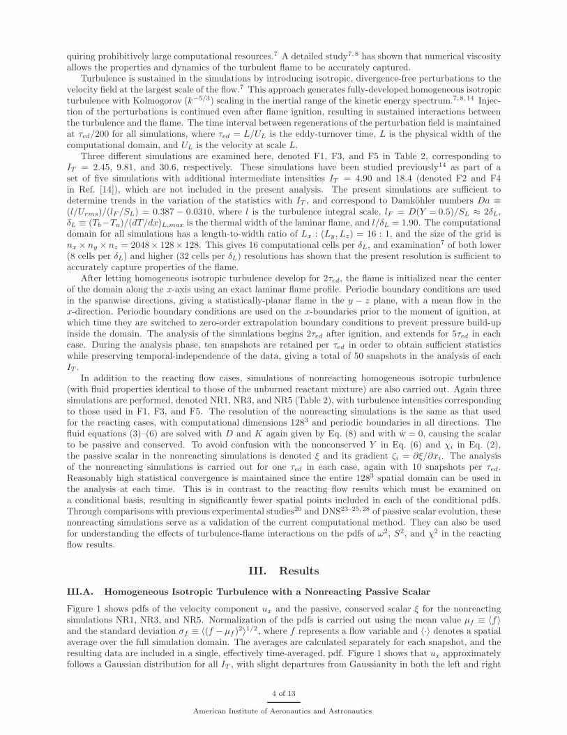
Figure 1 shows pdfs of the velocity component ux and the passive, conserved scalar ξ for the nonreactingsimulations NR1, NR3, and NR5. Normalization of the pdfs is carried out using the mean value µf ≡ 〈f〉and the standard deviation σf ≡ 〈(f − µf )
2〉1/2, where f represents a flow variable and 〈·〉 denotes a spatialaverage over the full simulation domain. The averages are calculated separately for each snapshot, and theresulting data are included in a single, effectively time-averaged, pdf. Figure 1 shows that ux approximatelyfollows a Gaussian distribution for all IT , with slight departures from Gaussianity in both the left and right
4 of 13
American Institute of Aeronautics and Astronautics
−6 −4 −2 0 2 4 610
−7
10−6
10−5
10−4
10−3
10−2
10−1
100
pd
f
(ux − µu)/σu
NR1
NR3
(a)
NR5
−6 −4 −2 0 2 4 610
−7
10−6
10−5
10−4
10−3
10−2
10−1
100
( ξ − µξ)/σ ξ
(b )
Figure 1. Pdfs of (a) (ux − µu)/σu and (b) (ξ − µξ)/σξ for nonreacting simulations NR1, NR3, and NR5. Dashed blacklines show Gaussian distributions.
tails. Similar results are observed for ξ in Figure 1, again with deviations from the Gaussian distribution inthe tails. The approximate Gaussianity of both ux and ξ for all IT in Figure 1, including the departures fromGaussianity at the tails, is consistent with prior studies23, 24 of passive scalars in nonreacting turbulence.
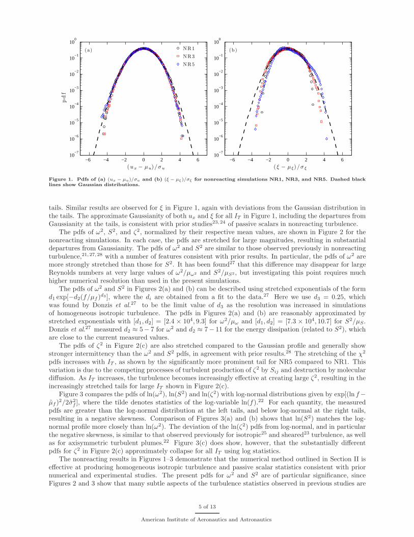
The pdfs of ω2, S2, and ζ2, normalized by their respective mean values, are shown in Figure 2 for thenonreacting simulations. In each case, the pdfs are stretched for large magnitudes, resulting in substantialdepartures from Gaussianity. The pdfs of ω2 and S2 are similar to those observed previously in nonreactingturbulence,21, 27, 28 with a number of features consistent with prior results. In particular, the pdfs of ω2 aremore strongly stretched than those for S2. It has been found27 that this difference may disappear for largeReynolds numbers at very large values of ω2/µω2 and S2/µS2 , but investigating this point requires muchhigher numerical resolution than used in the present simulations.
The pdfs of ω2 and S2 in Figures 2(a) and (b) can be described using stretched exponentials of the formd1 exp[−d2(f/µf )
d3 ], where the di are obtained from a fit to the data.27 Here we use d3 = 0.25, whichwas found by Donzis et al.27 to be the limit value of d3 as the resolution was increased in simulationsof homogeneous isotropic turbulence. The pdfs in Figures 2(a) and (b) are reasonably approximated bystretched exponentials with [d1, d2] = [2.4 × 10⁴, 9.3] for ω2/µω and [d1, d2] = [7.3 × 10⁴, 10.7] for S2/µS .Donzis et al.27 measured d2 ≈ 5− 7 for ω2 and d2 ≈ 7− 11 for the energy dissipation (related to S2), whichare close to the current measured values.
The pdfs of ζ2 in Figure 2(c) are also stretched compared to the Gaussian profile and generally showstronger intermittency than the ω2 and S2 pdfs, in agreement with prior results.28 The stretching of the χ2
pdfs increases with IT , as shown by the significantly more prominent tail for NR5 compared to NR1. Thisvariation is due to the competing processes of turbulent production of ζ2 by Sij and destruction by moleculardiffusion. As IT increases, the turbulence becomes increasingly effective at creating large ζ2, resulting in theincreasingly stretched tails for large IT shown in Figure 2(c).
Figure 3 compares the pdfs of ln(ω2), ln(S2) and ln(ζ2) with log-normal distributions given by exp[(ln f−µf )
2/2σ2f ], where the tilde denotes statistics of the log-variable ln(f).22 For each quantity, the measured
pdfs are greater than the log-normal distribution at the left tails, and below log-normal at the right tails,resulting in a negative skewness. Comparison of Figures 3(a) and (b) shows that ln(S2) matches the log-normal profile more closely than ln(ω2). The deviation of the ln(ζ2) pdfs from log-normal, and in particularthe negative skewness, is similar to that observed previously for isotropic25 and sheared23 turbulence, as wellas for axisymmetric turbulent plumes.22 Figure 3(c) does show, however, that the substantially differentpdfs for ζ2 in Figure 2(c) approximately collapse for all IT using log statistics.
The nonreacting results in Figures 1–3 demonstrate that the numerical method outlined in Section II iseffective at producing homogeneous isotropic turbulence and passive scalar statistics consistent with priornumerical and experimental studies. The present pdfs for ω2 and S2 are of particular significance, sinceFigures 2 and 3 show that many subtle aspects of the turbulence statistics observed in previous studies are
5 of 13
American Institute of Aeronautics and Astronautics
0 20 40 60 80
10−6
10−4
10−2
100
pd
f
ω2/µω 2
(a)
0 20 40 60 80
10−6
10−4
10−2
100
S 2/µS2
NR1
NR3
(b )
NR5
0 20 40 60 80
10−6
10−4
10−2
100
ζ 2/µζ
(c )
Figure 2. Pdfs of (a) ω2/µω2 , (b) S2/µ
S2 , and (c) ζ2/µζ2
for NR1, NR3, and NR5. Stretched exponentials
d1 exp[−d2(f/µf )0.25] are shown by green dashed lines in (a) and (b).
black lines show Gaussian distributions of log variables.
reproduced by solving Eqs. (3)–(6) with numerical viscosity and the grid resolution used in this work. Thequalitative agreement with prior results supports the use of the present numerical method in examiningintermittency effects in premixed flames, and the pdfs in Figures 1–3 are used for comparison with thereacting flow results in the next section.
III.B. Premixed Turbulent Combustion
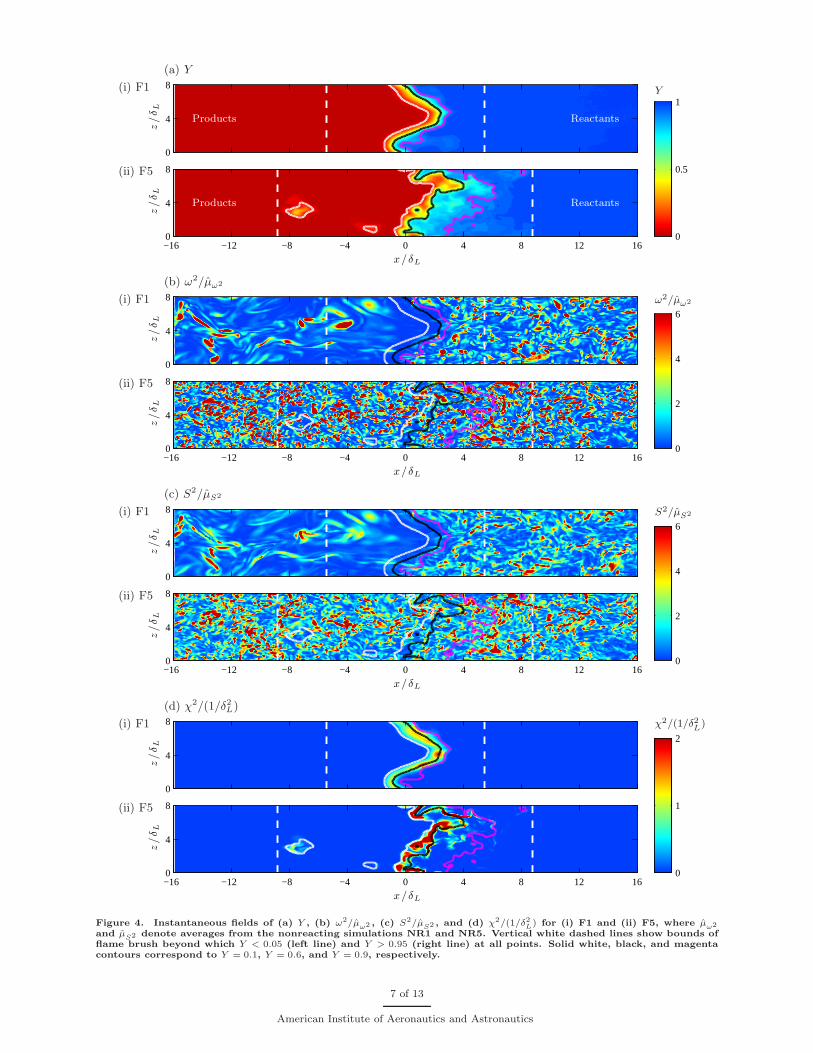
Figure 4 shows instantaneous fields of Y , ω2, S2, and χ2 for F1 and F5. The contours of Y in Figure 4(a)indicate that the flame is more wrinkled near the reactants than the products, and the degree of wrinklingthroughout the flame increases with IT . The separation between the Y = 0.6 and Y = 0.9 contours increasesfrom F1 to F5, which is indicative of increased flame broadening in the preheat zone. The width of thereaction zone (given by the separation between the Y = 0.1 and Y = 0.6 contours) remains relativelyunchanged as IT increases, in agreement with previous studies.7, 8, 14
Figures 4(b) and (c) show that ω2 and S2 are both suppressed within the flame brush for F1, but as ITincreases, this suppression is lost. The bounds of the flame brush are defined as the maximum (minimum)x locations to the left (right) of which Y < 0.05 (Y > 0.95) at all points. The suppression of ω2 and S2
extends beyond the flame brush into the products for F1. These fields are characterized at all locations andfor both F1 and F5 by localized regions of large magnitudes, although these magnitudes are larger comparedto the mean for ω2 than S2. Figure 4(c) shows that χ2 is zero in the reactants and products, since Y isconstant in these regions. Within the flame brush, there are thin regions of large χ2 inside the reaction zone(between the Y = 0.6 and Y = 0.1 contours).
Quantitative analysis of the fields in Figure 4 is complicated by the substantial spatial inhomogeneityof the flame brush. In particular, comparison of the intermittency at different locations within the flame,which is seen in Figure 4(a) to be highly wrinkled for large IT , requires calculation of conditional pdfs based
6 of 13
American Institute of Aeronautics and Astronautics
z/δ
L0
4
8
z/δ
L
x/δL
−16 −12 −8 −4 0 4 8 12 160
4
8
0
0.5
1
(a) Y
(i) F1
(ii) F5
Y
Products Reactants
Products Reactants
z/δ
L
0
4
8
z/δ
L
x/δL
−16 −12 −8 −4 0 4 8 12 160
4
8
0
2
4
6
(b) ω2/µω2
(i) F1
(ii) F5
ω2/µω2
z/δ
L
0
4
8
z/δ
L
x/δL
−16 −12 −8 −4 0 4 8 12 160
4
8
0
2
4
6
(c) S2/µS2
(i) F1
(ii) F5
S2/µS2
z/δ
L
0
4
8
z/δ
L
x/δL
−16 −12 −8 −4 0 4 8 12 160
4
8
0
1
2
(d) χ2/(1/δ2L)
(i) F1
(ii) F5
χ2/(1/δ2L)
Figure 4. Instantaneous fields of (a) Y , (b) ω2/µω2 , (c) S2/µ
S2 , and (d) χ2/(1/δ2L) for (i) F1 and (ii) F5, where µω2
and µS2 denote averages from the nonreacting simulations NR1 and NR5. Vertical white dashed lines show bounds of
flame brush beyond which Y < 0.05 (left line) and Y > 0.95 (right line) at all points. Solid white, black, and magentacontours correspond to Y = 0.1, Y = 0.6, and Y = 0.9, respectively.
7 of 13
American Institute of Aeronautics and Astronautics
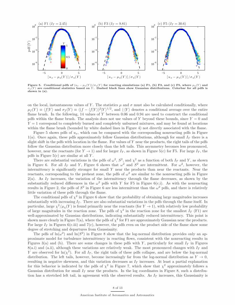
−5 0 5
10−6
10−4
10−2
100
[ux − µu(Y ) ] /σu(Y )
Y
0
0.5
1
(a) F1 (IT = 2.45)
pdf(Y)
−5 0 5
10−6
10−4
10−2
100
[ux − µu(Y ) ] /σu(Y )
(b) F3 (IT = 9.81)
−5 0 5
10−6
10−4
10−2
100
[ux − µu(Y ) ] /σu(Y )
(c) F5 (IT = 30.6)
Figure 5. Conditional pdfs of (ux − µu(Y ))/σu(Y ) for reacting simulations (a) F1, (b) F3, and (c) F5, where µu(Y ) andσu(Y ) are conditional statistics based on Y . Dashed black lines show Gaussian distributions. Colorbar for all pdfs isshown in (a).
on the local, instantaneous values of Y . The statistics µ and σ must also be calculated conditionally, whereµf (Y ) ≡ 〈f |Y 〉 and σf (Y ) ≡ 〈(f − 〈f |Y 〉)2|Y 〉1/2, and 〈·|Y 〉 denotes a conditional average over the entireflame brush. In the following, 14 values of Y between 0.06 and 0.94 are used to construct the conditionalpdfs within the flame brush. The analysis does not use values of Y beyond these bounds, since Y = 0 andY = 1 correspond to completely burned and completely unburned mixtures, and may be found at locationswithin the flame brush (bounded by white dashed lines in Figure 4) not directly associated with the flame.
Figure 5 shows pdfs of ux, which can be compared with the corresponding nonreacting pdfs in Figure1(a). Once again, these pdfs approximately follow Gaussian distributions, although for small IT there is aslight shift in the pdfs with location in the flame. For values of Y near the products, the right tails of the pdfsfollow the Gaussian distribution more closely than the left tails. This asymmetry becomes less pronounced,however, near the reactants (for Y → 1) and for larger IT , as shown in Figure 5(c) for F5. For large IT , thepdfs in Figure 5(c) are similar at all Y .
There are substantial variations in the pdfs of ω2, S2, and χ2 as a function of both IT and Y , as shownin Figure 6. For all IT and Y , Figure 6 shows that ω2 and S2 are intermittent. For ω2, however, theintermittency is significantly stronger for small Y near the products than near the reactants. Near thereactants, corresponding to the preheat zone, the pdfs of ω2 are similar to the nonreacting pdfs in Figure2(a). As IT increases, the variation of the intermittency through the flame decreases, as shown by thesubstantially reduced differences in the ω2 pdfs with Y for F5 in Figure 6(c.i). As with the nonreactingresults in Figure 2, the pdfs of S2 in Figure 6 are less intermittent than the ω2 pdfs, and there is relativelylittle variation of these pdfs through the flame.
The conditional pdfs of χ2 in Figure 6 show that the probability of obtaining large magnitudes increasessubstantially with increasing IT . There are also substantial variations in the pdfs through the flame itself. Inparticular, large χ2/µχ(Y ) is found primarily near the reactants (for Y → 1), with relatively low probabilityof large magnitudes in the reaction zone. The pdfs of χ2 in the reaction zone for the smallest IT (F1) arewell-approximated by Gaussian distributions, indicating substantially reduced intermittency. This point isshown more clearly in Figure 7(a), where the pdfs of χ2 for F1 are approximately Gaussian near the products.For large IT in Figures 6(c.iii) and 7(c), however, the pdfs even on the product side of the flame show somedegree of stretching and departures from Gaussianity.
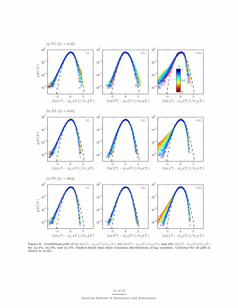
The pdfs of ln(ω2) and ln(S2) in Figure 8 show that the log-normal distribution provides only an ap-proximate model for turbulence intermittency in reacting flows, consistent with the nonreacting results inFigures 3(a) and (b). There are some changes in these pdfs with Y , particularly for small IT in Figures8(a.i) and (a.ii), although these variations are relatively weak. The most pronounced changes with IT andY are observed for ln(χ2). For all IT , the right tails of these pdfs collapse, and are below the log-normaldistribution. The left tails, however, become increasingly far from the log-normal distribution as Y → 0,resulting in negative skewness, and this variation decreases as IT increases. At least a partial explanationfor this behavior is indicated by the pdfs of χ2 in Figure 7, which show that χ2 approximately follows aGaussian distribution for small IT near the products. In the log coordinates in Figure 8, such a distribu-tion has a stretched left tail, in agreement with the observed results. As IT increases, this Gaussianity is
8 of 13
American Institute of Aeronautics and Astronautics
0 20 40 60 80
10−6
10−4
10−2
100
pd
f(Y
)
ω2/µω 2(Y )
( i )
0 20 40 60 80
10−6
10−4
10−2
100
S 2/µS2(Y )
( i i )
0 20 40 60 80
10−6
10−4
10−2
100
χ2/µχ2(Y )
( i i i )
Y
0
0.5
1
(a) F1 (IT = 2.45)
0 20 40 60 80
10−6
10−4
10−2
100
pd
f(Y
)
ω2/µω 2(Y )
( i )
0 20 40 60 80
10−6
10−4
10−2
100
S 2/µS2(Y )
( i i )
0 20 40 60 80
10−6
10−4
10−2
100
χ2/µχ2(Y )
( i i i )
(b) F3 (IT = 9.81)
0 20 40 60 80
10−6
10−4
10−2
100
pd
f(Y
)
ω2/µω 2(Y )
( i )
0 20 40 60 80
10−6
10−4
10−2
100
S 2/µS2(Y )
( i i )
0 20 40 60 80
10−6
10−4
10−2
100
χ2/µχ2(Y )
( i i i )
(c) F5 (IT = 30.6)
Figure 6. Conditional pdfs of (i) ω2/µω2 (Y ), (ii) S2/µ
S2 (Y ), and (iii) ζ2/µζ2
(Y ) for (a) F1, (b) F3, and (c) F5. The
stretched exponentials d1 exp[−d2(f/µf )0.25] from the nonreacting results in Figure 2 are shown by black dashed lines in
(i) and (ii). Colorbar for all pdfs is shown in (a.iii).
9 of 13
American Institute of Aeronautics and Astronautics
−5 0 5
10−6
10−4
10−2
100
[χ2− µχ2(Y ) ] /σχ2(Y )
Y
0
0.5
1
(a) F1 (IT = 2.45)
pdf(Y)
−5 0 5
10−6
10−4
10−2
100
[χ2− µχ2(Y ) ] /σχ2(Y )
(b) F3 (IT = 9.81)
−5 0 5
10−6
10−4
10−2
100
[χ2− µχ2(Y ) ] /σχ2(Y )
(c) F5 (IT = 30.6)
Figure 7. Conditional pdfs of (χ2− µ
χ2 (Y ))/σχ2 (Y ) for reacting simulations (a) F1, (b) F3, and (c) F5. Dashed black
lines show Gaussian distributions. Colorbar for all pdfs is shown in (a).
lost and the left tails increasingly conform to the nonreacting distribution shown in Figure 3. It should beemphasized, however, that the log-normal distribution is in general not an accurate representation of the χ2
pdfs in premixed flames. For all IT , the log pdfs are characterized by negative skewness and departures fromlog-normality, consistent with previous observations in both nonreacting22, 23, 25, 39 and reacting29 flows.
IV. Discussion and Conclusions
The present study has examined the pdfs of ω2, S2, and χ2 in premixed H2-air flames. These pdfsare studied as a function of turbulence intensity, IT , and location in the flame using conditional statisticsbased on the local, instantaneous values of Y . The analysis is based on DNS of statistically-planar flames atthree different values of IT . Simulations of nonreacting homogeneous isotropic turbulence with a conserved,passive scalar have also been carried out in order to validate the numerical method and allow comparisonswith the reacting flow results. The qualitative properties of the nonreacting ω2, S2, and ζ2 pdfs are foundto be consistent with prior numerical23–28 and experimental20–22 studies.
The reacting flow results in Figures 6–8 show that there are substantial variations in the pdfs of ω2 andS2 with both IT and location in the flame. For large IT , the pdfs of ω
2 and S2 are similar to the nonreactingpdfs in Figures 2 and 3. This suggests that the turbulence intermittency is relatively unaffected by the flamewhen IT is large, consistent with prior observations of premixed turbulence-flame interactions.14, 40 Forsmall IT , however, the pdfs of ω2 undergo substantial variations through the flame, with more pronouncedstretching of the pdf tails near the products. The suppression of average ω2 in flames for small IT hasbeen observed previously,14, 40–42 and is due to dilatational effects resulting from chemical energy release.The present results further suggest that the fluctuations about the mean, and the associated intermittency,increase from the reactants to the products. In general, weaker variations were observed in the pdfs of S2,possibly due to the presence of a mean velocity gradient along the mean flow direction (x) caused by fluidexpansion.
Figures 6–8 show that the pdfs of χ2 also undergo substantial changes with IT and position in the flame.For all IT , the pdfs are stretched to larger values of χ2/µχ2(Y ) near the reactants, and for moderate andlarge values of IT , the pdfs near the products are also intermittent. The range of observed χ2/µχ2(Y )increases with IT for all Y , consistent with the increases observed in Figure 2 for the nonreacting turbulencesimulations. As with the nonreacting simulations, this increase is associated with greater dominance ofturbulence over chemical and molecular diffusion processes when IT is large. For small IT , Figures 6–8 showthat the pdfs of χ2 approach a Gaussian distribution in the reaction zone, indicative of substantially reducedintermittency. The pdfs of χ2 for the smallest value of IT examined in the present study (F1) thus vary froman essentially non-intermittent Gaussian distribution near the products to an intermittent distribution nearthe reactants. The source and physical meaning of this Gaussianity requires further investigation.
It should be noted that the pdfs of ω2, S2, and χ2 (or ζ2 in the passive scalar case) are, in general, relativelypoorly approximated by log-normal distributions for all IT and Y . Log-normality is only one of severalpossible models for intermittent pdfs,11, 18 however, and comparisons with different modeled forms deserve
10 of 13
American Institute of Aeronautics and Astronautics
−5 0 5
10−6
10−4
10−2
100
pd
f(Y
)
[ l n(ω2) − µω 2(Y ) ] / σω 2(Y )
( i )
−5 0 5
10−6
10−4
10−2
100
[ l n(S 2) − µS2(Y ) ] / σS2(Y )
( i i )
−5 0 5
10−6
10−4
10−2
100
[ l n(χ2) − µχ2(Y ) ] / σχ2(Y )
( i i i )
Y
0
0.5
1
(a) F1 (IT = 2.45)
−5 0 5
10−6
10−4
10−2
100
pd
f(Y
)
[ l n(ω2) − µω 2(Y ) ] / σω 2(Y )
( i )
−5 0 5
10−6
10−4
10−2
100
[ l n(S 2) − µS2(Y ) ] / σS2(Y )
( i i )
−5 0 5
10−6
10−4
10−2
100
[ l n(χ2) − µχ2(Y ) ] / σχ2(Y )
( i i i )
(b) F3 (IT = 9.81)
−5 0 5
10−6
10−4
10−2
100
pd
f(Y
)
[ l n(ω2) − µω 2(Y ) ] / σω 2(Y )
( i )
−5 0 5
10−6
10−4
10−2
100
[ l n(S 2) − µS2(Y ) ] / σS2(Y )
( i i )
−5 0 5
10−6
10−4
10−2
100
[ l n(χ2) − µχ2(Y ) ] / σχ2(Y )
( i i i )
(c) F5 (IT = 30.6)
Figure 8. Conditional pdfs of (i) [ln(ω2)− µω2 (Y )]/σ
ω2 (Y ), (ii) [ln(S2)− µS2(Y )]/σ
S2(Y ), and (iii) [ln(χ2)− µχ2 (Y )]/σ
χ2 (Y )
for (a) F1, (b) F3, and (c) F5. Dashed black lines show Gaussian distributions of log variables. Colorbar for all pdfs isshown in (a.iii).
11 of 13
American Institute of Aeronautics and Astronautics
future consideration. The pronounced negative skewness of the ln(χ2) pdfs shown in Figures 3(c) and 6(iii)has received particular attention in previous studies of the scalar dissipation, including for planar turbulentjets,39 axisymmetric plumes,22 and piloted jet flames.29 Su and Clemens39 have provided a systematicanalysis of this skewness, and ultimately conclude that it is a physical feature of scalar dissipation pdfs.This skewness has been represented previously22, 29 using exponential distributions for the left tails of theln(χ2) pdfs, and future work will determine the conformity of the present premixed flame results to thesedistributions.
Acknowledgments
This work was supported by the National Research Council Research Associateship Program, the NavalResearch Laboratory through the Office of Naval Research, and by the Air Force Office of Scientific Re-search. Computing facilities were provided by the Department of Defense High Performance ComputingModernization Program.
References
1Pope, S., “Turbulent premixed flames.” Ann. Rev. Fluid Mech., Vol. 19, 1987, pp. 237–270.2Bilger, R. W., “Future progress in turbulent combustion research.” Prog. Ener. Comb. Sci., Vol. 26, 2000, pp. 367–380.3Chakraborty, N., Rogerson, J. W., and Swaminathan, N., “The scalar gradient alignment statistics of flame kernels and
its modelling implications for turbulent premixed combustion.” Flow Turb. Combust., Vol. 85, 2010, pp. 25–55.4Poinsot, T. and Veynante, D., Theoretical and numerical combustion, Edwards, 2005.5Dunn, M. J., Masri, A. R., and Bilger, R. W., “A new piloted premixed jet burner to study strong finite-rate chemistry
effects.” Combust. Flame, Vol. 151, 2007, pp. 46–60.6Aspden, A. J., Bell, J. B., Day, M. S., Woosley, S. E., and Zingale, M., “Turbulence-Flame Interactions in Type Ia
Supernovae.” Astrophys. J., Vol. 689, 2008, pp. 1173–1185.7Poludnenko, A. Y. and Oran, E. S., “The interaction of high-speed turbulence with flames: Global properties and internal
flame structure.” Comb. Flame, Vol. 157, 2010, pp. 995–1011.8Poludnenko, A. Y. and Oran, E. S., “The interaction of high-speed turbulence with flames: Turbulent flame speed.”
Comb. Flame, In Press, ISSN 0010-2180, DOI: 10.1016/j.combustflame.2010.09.002 , 2010.9Bilger, R. W., “Some aspects of scalar dissipation.” Flow Turb. Combust., Vol. 72, 2004, pp. 93–114.
10Sreenivasan, K., “Possible effects of small-scale intermittency in turbulent reacting flows.” Flow Turb. Combust., Vol. 72,2004, pp. 115–131.
11Pan, L., Wheeler, J. C., and Scalo, J., “The effect of turbulent intermittency on the deflagration to detonation transitionin supernova Ia explosions.” Astrophys. J., Vol. 681, 2008, pp. 470–481.
12Tsinober, A., An Informal Conceptual Introduction to Turbulence, Springer, 2009.13Kim, S. H. and Pitsch, H., “Scalar gradient and small-scale structure in turbulent premixed combustion.” Phys. Fluids,
Vol. 19, 2007, 115104.14Hamlington, P. E., Poludnenko, A. Y., and Oran, E. S., “Turbulence and scalar gradient dyanmics in premixed reacting
flows.” AIAA Paper 2010-5027 , 2010.15Swaminathan, N. and Grout, R. W., “Interaction of turbulence and scalar fields in premixed flames.” Phys. Fluids,
Vol. 18, 2006, 045102.16Chakraborty, N. and Swaminathan, N., “Influence of the Damkohler number on turbulence-scalar ineraction in premixed
flames. I. Physical insight.” Phys. Fluids, Vol. 19, 2007, 045103.17Hartung, G., Hult, J., Kaminski, C. F., Rogerson, J. W., and Swaminathan, N., “Effect of heat release on turbulence
and scalar-turbulence interaction in premixed combustion.” Phys. Fluids, Vol. 20, 2008, 035110.18Frisch, U., Turbulence: The Legacy of A.N. Kolmogorov , Cambridge University Press, 1995.19Davidson, P. A., Turbulence: An Introduction for Scientists and Engineers, Oxford University Press, 2004.20Su, L. K. and Dahm, W. J. A., “Scalar imaging velocimetry measurements of the velocity gradient tensor field in turbulent
flows. II. Experimental results,” Phys. Fluids, Vol. 8, 1996, pp. 1883–1906.21Zeff, B. W., Lanterman, D. D., McAllister, R., R. Roy, E. J. K., and Lathrop, D. P., “Measuring intense rotation and
dissipation in turbulent flows,” Nature, Vol. 421, 2003, pp. 146–149.22Markides, C. N. and Mastorakos, E., “Measurements of the statistical distribution of the scalar dissipation rate in
turbulent axisymmetric plumes.” Flow. Turb. Combust., Vol. 81, 2008, pp. 221–234.23Miller, R. S., Jaberi, F. A., Madnia, C. K., and Givi, P., “The structure and small-scale intermittency of passive scalars
in homogeneous turbulence.” J. Sci. Comp., Vol. 10, 1995, pp. 151–180.24Overholt, M. R. and Pope, S. B., “Direct numerical simulation of a passive scalar with improsed mean gradient in isotropic
turbulence.” Phys. Fluids, Vol. 8 (11), 1996, pp. 3128–3148.25Vedula, P., Yeung, P. K., and Fox, R. O., “Dynamics of scalar dissipation in isotropic turbulence: a numerical and
modelling study.” J. Fluid Mech., Vol. 433, 2001, pp. 29–60.26Schumacher, J., Sreenivasan, K. R., and Yeung, P. K., “Very fine structures in scalar mixing.” J. Fluid Mech., Vol. 531,
2005, pp. 113–122.
12 of 13
American Institute of Aeronautics and Astronautics
27Donzis, D. A., Yeung, P. K., and Sreenivasan, K. R., “Dissipation and enstrophy in isotropic turbulence: Resolutioneffects and scaling in direct numerical simulations,” Phys. Fluids, Vol. 20, 2008, 045108.
28Donzis, D. A. and Yeung, P. K., “Resolution effects and scaling in numerical simulations of passive scalar mixing inturbulence.” Physica D , Vol. 239, 2010, pp. 1278–1287.
29Karpetis, A. N. and Barlow, R. S., “Measurements of scalar dissipation in a turbulent piloted methane/air jet flame.”Proc. Comb. Inst., Vol. 29, 2002, pp. 1929–1936.
30Bilger, R. W., “Turbulent jet diffusion flames.” Prog. Energy. Combust. Sci., Vol. 1, 1976, pp. 87–109.31Bray, K. N. C., in: P. A. Libby and F. A. Williams (Eds.), Turbulent Reacting Flows, Springer-Verlag, New York, 1980.32Swaminathan, N. and Bray, K. N. C., “Effect of dilatation on scalar dissipation in turbulent premixed flames.” Comb.
Flame, Vol. 143, 2005, pp. 549–565.33Pope, S. B., Turbulent Flows, Cambridge University Press., 2000.34Stone, J. M., Gardiner, T. A., Teuben, P., Hawley, J. F., and Simon, J. B., “Athena: A New Code for Astrophysical
MHD.” Astrophys. J. Supp., Vol. 178, 2008, pp. 137–177.35Gardiner, T. A. and Stone, J. M., “An unsplit Godunov method for ideal MHD via constrained transport in three
dimensions.” J. Comp. Phys., Vol. 227, 2008, pp. 4123–4141.36Gamezo, V., Ogawa, T., and Oran, E., “Flame acceleration and DDT in channels with obstacles: Effect of obstacle
spacing.” Comb. Flame, Vol. 155, 2008, pp. 302–315.37Colella, P., “Multidimensional upwind methods for hyperbolic conservation-laws.” J. Comp. Phys., Vol. 87, 1990, pp. 171–
200.38Saltzman, J., “An Unsplit 3D Upwind Method for Hyperbolic Conservation-Laws.” J. Comp. Phys., Vol. 115, 1994,
pp. 153–168.39Su, L. K. and Clemens, N. T., “The structure of fine-scale scalar mixing in gas-phase planar turbulent jets.” J. Fluid
Mech., Vol. 488, 2003, pp. 1–29.40Mueller, C., Driscoll, J., Reuss, D., Drake, M., and Rosalik, M., “Vorticity generation and attenuation as vortices convect
through a premixed flame,” Comb. Flame, Vol. 112, 1998, pp. 342–358.41McMurtry, P., Riley, J., and Metcalfe, R., “Effects of heat release on the large-scale structure in turbulent mixing layers.”
J. Fluid Mech., Vol. 199, 1989, pp. 297–332.42Lipatnikov, A. and Chomiak, J., “Effects of premixed flames on turbulence and turbulence scalar transport.” Prog. Ener.
Comb. Sci., Vol. 36, 2010, pp. 1–202.
13 of 13
American Institute of Aeronautics and Astronautics