Page 1
1
Intermittent missing measurements in longitudinal study of physical growth of children:
Is it necessary to impute?
Esnat Dorothy Chirwa1,2
*Corresponding Author
Email: [email protected]
Paula Griffiths 2,3
Email: [email protected]
Shane A Norris
2
Email: [email protected]
Ken Maleta4
Email: [email protected]
Per Ashorn5
Email: [email protected]
Noel Cameron 2,3
Email: [email protected]
1Department of Mathematical Sciences, Chancellor College, University of Malawi.
2Wits/MRC Developmental Pathways for Health Research Unit, School of Clinical Medicine,
Faculty of Health Sciences, University of the Witwatersrand, Johannesburg, South Africa.
3Centre for Global Health and Human Development, Loughborough University,
Loughborough,
Leicestershire, LE 11 3TU, UK.
4Department of Community Health, College of Medicine, University of Malawi.
5Department of International Health, School of Medicine, University of Tampere, Finland and
Department of Paediatrics, Tampere University Hospital, Finland.
Page 2
2
ABSTRACT.
Background: Missing data in longitudinal studies are inevitable. Despite the existence of
various statistical methods that deal with missing data in longitudinal studies in general, it is
important to consider the nature of the repeated measurements in selecting such methods. This
paper aims to compare effectiveness of multiple imputation (MI) or growth-model based
Regression Imputation (RI) in handling intermittent missing physical child growth data.
Methods: Longitudinal measurements of weight and height from South African and
Malawian child growth cohorts were used. Missing data patterns in the cohorts were introduced
in the complete data to create intermittent missing data. The complete dataset was used to
provide a reference point for the accuracy of the different methods of handling with missing
data. The Berkey-Reed 1st order growth model was fitted using Linear Mixed Effects (LME)
models. Relative bias of the parameter estimates of this child growth model and mean square
errors were used to assess the added value of using MI or RI in handling intermittent missing
data compared to a model fitted to data with missing measurements.
Results: There were no statistically significant differences in parameter estimates between RI,
Available Case Analysis (ACA) or MI within both cohorts. However there were large biases in
parameter estimates in South African cohort (weight: 0.91 < mean RBIAS< 5.97; height: 2.54<
mean RBIAS<46.5). There were no significant differences in observed, interpolated or multiple
imputed weight and height measurements in both cohorts (0.001<|mean diff|<0.21; 0.11< p-
values <0.98).
Conclusions: The study shows little added value in imputing for intermittent missing data in
physical growth measurements. However, MI helped deal with convergence problems created
by the imbalance due to missing data, when time interval between data points is large.
Page 3
3
KEYWORDS: Missing data, Multiple Imputation, RI, linear mixed models,
longitudinal measurements
Page 4
4
BACKGROUND
One of the main challenges in the analysis of data from studies that involve repeated
measurements over time such as growth monitoring studies is the inevitability of missing
information. Missing data in studies of physical growth can arise due to participants being lost
to follow up due to migration, dropping out or missing scheduled visits. Ignoring individuals
with missing data in the analysis of such longitudinal studies by using a complete case analysis
(CCA) can lead to biased results, especially if the individuals with missing data have different
characteristics to those with complete data. In longitudinal studies, CCA can also lead to a
substantially reduced sample size, especially where there are a large number of data waves,
thus leading to loss of power (Engels and Diehr 2003; Blankers, Koeter et al. 2010).
Researchers have used different methods to deal with missing data in longitudinal studies
and these include imputing the missing information, analysing ignoring individuals with
missing information or analysing the data using the available partial information. Whether to
impute or not, and which imputation method to use, depends on the reason for analysis, the
type of variable, the amount of missing data and the pattern of missing data (intermittent or
monotonic) (Mallinckrodt, Sanger et al. 2003; Sterne, White et al. 2009).
The risk of bias in estimates and the magnitude of the effect due to CCA depends on the
mechanism behind the missing data patterns as defined by Little and Rubin (Little and Rubin
2002; Mallinckrodt, Sanger et al. 2003; Sterne, White et al. 2009). Under missing completely
at random (MCAR) and missing at random (MAR), ignoring cases with missing data can still
produce valid results. The major concern would be the reduced sample size which can lead to
loss of power. However, if data are missing not at random (MNAR), ignoring cases with
missing data would lead to biased estimates and, thus, affect the validity of the findings (Twisk
and de Vente 2002; Blankers, Koeter et al. 2010). Further, it is usually difficult to distinguish
Page 5
5
between MAR and MNAR since MNAR depends on unobserved data (Sterne, White et al.
2009; Grittner, Gmel et al. 2011).
Researchers have used different methods to impute for missing data in longitudinal studies.
These methods range from ones that use population group information to those that use the
longitudinal nature of the data in each case, such as Last Observation Carried Forward (LOCF),
and linear interpolation (Twisk and de Vente 2002; Engels and Diehr 2003; Tang, Song et al.
2005; Grittner, Gmel et al. 2011). Although studies have shown that in general, methods that
use the longitudinal nature of the data such as linear interpolation to impute values are better
than cross-sectional population based methods, applying them to physical growth data in
children might not be appropriate (Twisk and de Vente 2002; Engels and Diehr 2003; Grittner,
Gmel et al. 2011). Physical growth in children is characterised by rapid non-linear growth,
especially in infancy, thus applying linear interpolation to impute for missing growth
measurements might produce values that either grossly underestimate or overestimate the
measurements.
With advances in statistical software, Multiple Imputation (MI) has become one of the more
common methods used in dealing with bias due to loss of information from missing data. MI
allows for uncertainty about the missing data by creating a number of datasets in which all
missing values are replaced by the imputed values calculated based on some posterior
distribution (Engels and Diehr 2003; Spratt, Carpenter et al. 2010). While MI can help in
reducing bias, Carpenter et al cautions against its indiscriminate use (Carpenter, Kenward et al.
2007). They argue that MI, which is based on MAR assumption, can bring in some bias if the
imputation model is wrongly defined. Under MAR, the probability of missing values is related
to some observed variables. Thus, it is important to identify any factors associated with the
outcome and to include such factors in the imputation model (Kenward and Carpenter 2007;
Page 6
6
Sterne, White et al. 2009; He, Yucel et al. 2011). In child physical growth modelling, these
factors may include maternal and household characteristics that are known to affect child
growth. Apart from inclusion of the factors that affect growth in the imputation process, MI
may also be affected by the amount of information already available, i.e the number of data
points per participant (Graham 2009).
Advances in statistical methods have also enabled researchers to use the available
information in a data set to measure effects rather than excluding cases where any data are
missing. The Available Case Analysis (ACA) methods include Linear mixed effects (LME)
regression and generalised estimating equations (GEE). LME has been used in modelling
growth, since apart from the flexibility of including a random component to describe the
variations in individual growth profiles, the methods may be used to fit structural (parametric)
and non-structural (non-parametric) curves. The superiority of ACA methods over CCA is due
to the fact that ACA methods incorporate the partial information from cases with missing data.
However, the methods can also lead to biased results if missing data are not MAR. The
performance of the LME model will also depend on the amount of missing observations per
participant (Blankers, Koeter et al. 2010; Peters, Bots et al. 2012).
This study assessed whether in growth modelling it is necessary to impute for missing
physical growth measurements from infancy to late childhood and examined how the time
interval between data collection waves affects the performance of the different methods of
dealing with missing data in longitudinal growth monitoring studies. This study built upon
work by Peters et al (2010) which used linear mixed effects modelling to compare ACA and
MI with CCA using longitudinal measurements to assess the added value of performing MI in
dealing with missing data in repeated outcome measures of a longitudinal dataset. While the
study by Peters et al looked at the effect of changing the percentage of missing data, our study
Page 7
7
looked at whether data collection wave intensity affects the performance of the different
methods of dealing with longitudinal missing data.
METHODS
The study used weight and height measurements from 2 African cohorts. The Bone-Health
(BH) Study (a sub-sample of the Birth-to-Twenty (Bt20) birth cohort born in Soweto-
Johannesburg, South Africa), which includes 453 black participants. More specific details
about the cohort are reported elsewhere (Cameron, Pettifor et al. 2003; Cameron, Wright et al.
2005). This study uses anthropometric measurements at birth, 1year, 2 years, 4 years, 5 years,
7 years, 9 years and at10 years.
The Lungwena Child Survival Study (LCSS) is cohort study of about 770 children and is set
in Mangochi, a rural district in southern Malawi. The on-going study is unique in that it has
growth data of children who have been followed up from birth and are now about 16 to 17
years old. Unlike the BH study, data collection phases were more intensive. The
anthropometric data were collected monthly from birth until 18 months, 3 monthly until 60
months, then at 6 years, 8-9 years, 10 years, 12 years and 15 years. More specific details for the
Lungwena cohort are reported elsewhere (Espo, Kulmala et al. 2002; Maleta, Virtanen et al.
2003). This paper used 3 monthly data from birth to 60 months, and then at 6 years, 8-9 years
and 10 years to capture the childhood growth period. Only children with complete weight and
height measurements were used in the study (BH study=90, LCSS study=140).
Page 8
8
Missing data simulation
Patterns of missing data were first examined before assumptions of the mechanism behind
missing data were made. Even though, there were a high proportion of missing values at 3 and
6 months in the BH cohort, we did not think the probability of missing values at each data
collection wave depended on the weight or height measurements. Thus, assuming that data was
missing at random, missing values were then simulated for both cohorts (BH study and LCSS
study) by using subsamples and deleting some weight or height measurements in order to
achieve similar pattern in missingness as in the original dataset. Datasets were created with the
same percentage of missing values as the original dataset, which was around 20 %. To
investigate reliability and coverage of the results, 50 bootstrap samples were drawn from the
dataset with simulated missing data for weight and height measurements for each cohort,
giving a total of 200 datasets.
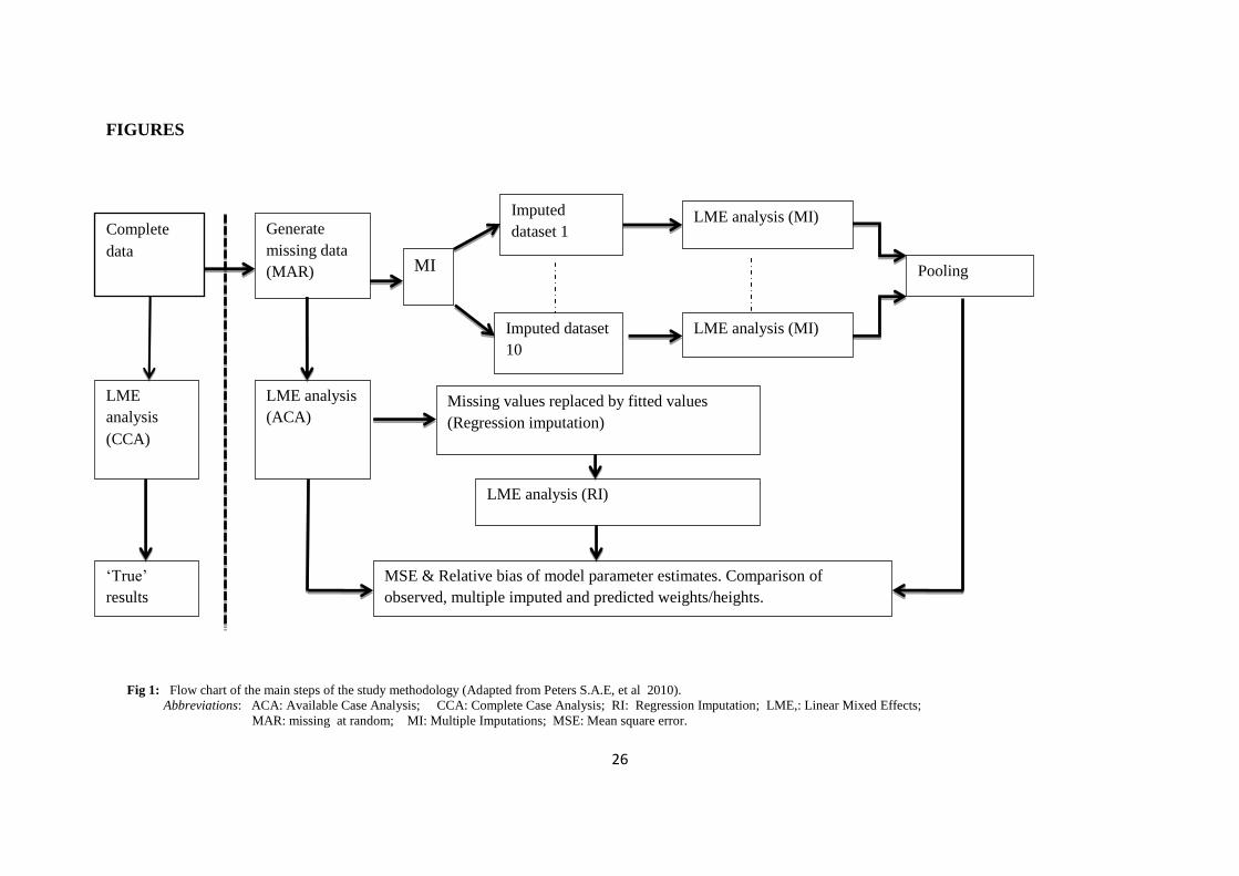
Figure 1 shows the flow chart of the study methodology used. For Multiple Imputation, 10
imputations for each missing value were done. The Berkey-Reed 1st order model, which is
used to describe physical growth in childhood and had previously been found to fit well to the
data, was used to model growth (Berkey and Reed 1987; Chirwa, Griffiths et al. 2014). The
model is defined as:
ij
ij
ijijijt
tty 1
)ln( 3210 kj ,....2,1 , ni ....2,1 (1)
where ijy = weight/height of child i at time point j.
ijt = age of child i at time point j.
The model was fitted to complete data, incomplete data, multiple imputed data and
interpolated data in each of the 50 datasets from both cohorts. Growth models were fitted to
Page 9
9
boys and girls separately, and were fitted using linear mixed effects (LME) modelling as
outlined in Fig.1.
To assess the effect of using MI, ACA or RI, parameter estimates of the growth model for each
method were compared with their corresponding parameter estimates from the original
complete data (CCA). The comparison was done using Relative Bias (RBIAS) of the growth
model coefficients and the root of relative mean square errors (RRMSE) as defined in He et al
(He 2010).
Relative bias is defined as RBIAS= |Bias/True| * 100%
where Bias= Coeff (Method) - Coeff(True).
The root of the relative mean square error is defined as RRMSE= )()(
TrueMSEMethodMSE .
The average of the relative biases and RRMSE were calculated from the 50 data sets. The
percentage coverage, which looked at the proportion of parameters from the 50 datasets, that
were within a 95 % confidence interval of their corresponding estimates derived from complete
data (CCA), were also used to compare the different methods of dealing with missing data.
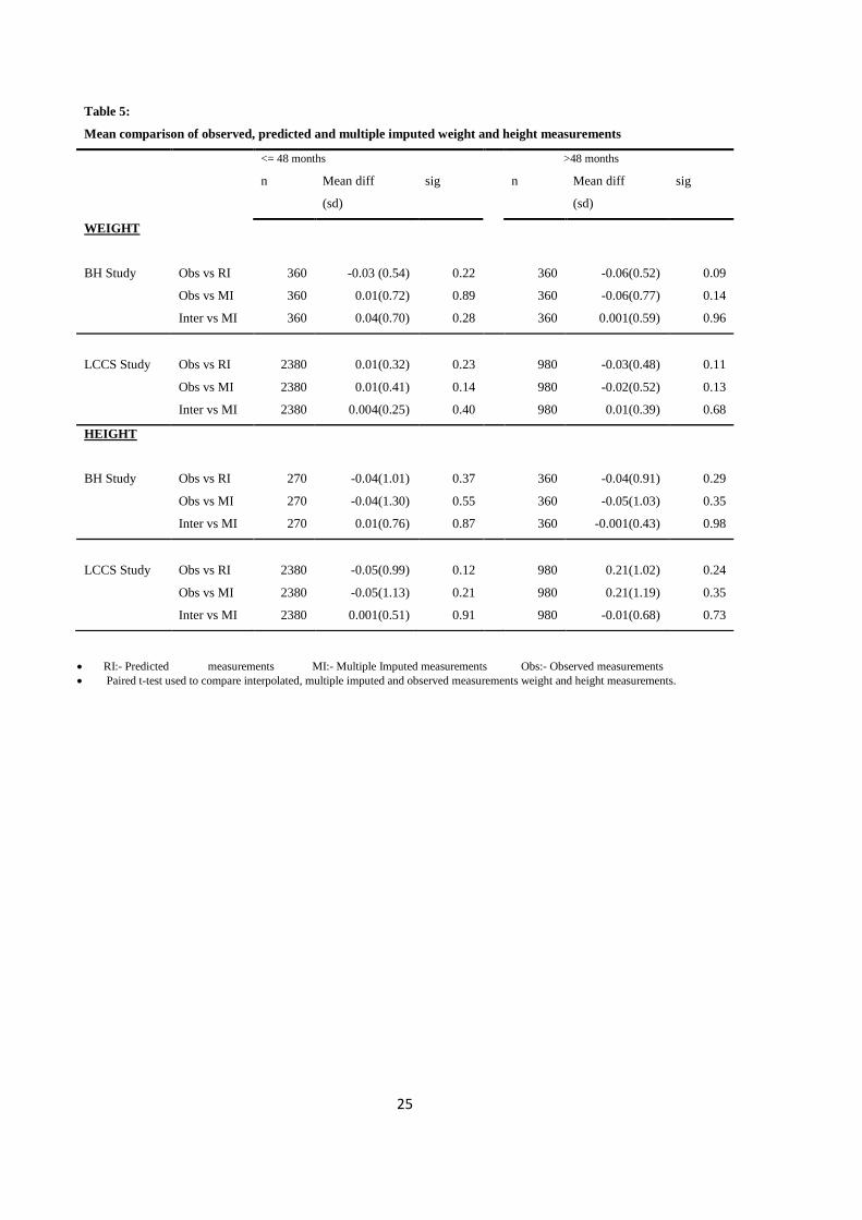
Paired t-tests were used to compare observed, predicted and multiple imputed weight and
height measurements.
[ insert Fig 1]
Page 10
10
RESULTS
Descriptive Analysis
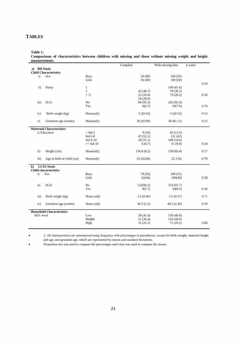
There were no significant differences in maternal, household and child characteristics, such as
sex of the child, birth-weight, maternal height, maternal age and SES-level, between complete
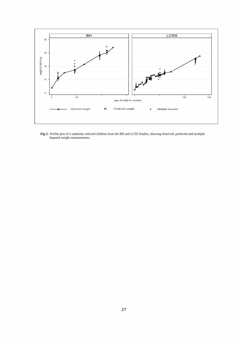
and incomplete cases for both cohorts (0.10<p-value< 0.78, Table 1). Growth profiles of a
random selection of children from the BH and LCSS studies (Fig 2), in general showed
interpolated values being closer to observed values than most multiple imputed values.
[insert Table 1 and Fig 2]
Modelling data from BH study
In modelling weight using data from the BH study, Multiple Imputation (MI) produced
parameter estimates that were on average slightly more biased than those derived from using
RI or the ACA method. The average RBIAS values for the MI were in general higher than
those derived using ACA or RI (Table 2). There were no significant differences in the RBIAS
of parameters between ACA and RI. Of the 50 estimates of the intercepts (Bo) derived using
MI, about 10 % were outside the 95% confidence limits of the intercept derived using the
original complete data. All parameter estimates derived using ACA or RI were within the 95%
confidence limits of the CCA parameters.
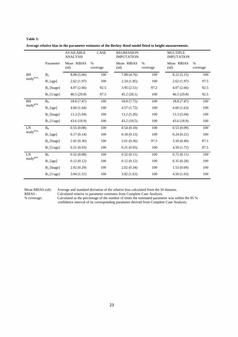
Consistent with results from the model for weight, parameter estimates from the RI method for
the height models were largely similar to the ACA parameter estimates, with average RBIAS
values from RI similar to those from the ACA method. However, standard errors for parameter
estimates from the RI method were consistently smaller than those from ACA. This is expected
since imputed values the RI method used were predicted values after fitting model to data with
Page 11
11
missing values (ACA method), thus reducing the variation in the measurements. The reduction
in the variation due to RI was also shown by the overall mean square errors (MSE) after fitting
the models. In both weight and height models, the MSE values for the RI analysis were
consistently smaller than those from the ACA method or MI method. Consistent with the
RBIAS values, the root of the relative mean square error (RRMSE) also showed no significant
differences in the estimates of the MSE between the ACA and RI methods. The large variation
in the MI values for the weight models were also shown by the larger MSE values from the MI
method relative to the other methods, giving RRMSE values that were greater than 1.
There is relatively more bias in the estimation of the coefficients of the ‘1/age’ and ‘ln(age’)’
terms of both weight and height models, indicating a general instability in the estimation of
these parameters by all the methods. The height models also produced high RBIAS values for
the estimate of the constant term (Bo), indicating increased variation in the estimation of the
initial individual height values of the children. This could be due to the model for height
starting at 1 year when measurements are more variable, rather than at birth as is the case with
the model for weight. Even though there were some biases in the parameter estimates of the 3
methods, paired t-tests showed no significant differences between observed, interpolated, or
average of multiple imputed measurements (Table 4).
[insert Table 2 & 3]
Page 12
12
Modelling data from LCSS Study
Consistent with BH study results, there were no significant differences in the parameter
estimates from the CCA, ACA, MI and RI methods when the Berkey-Reed model was fitted to
the Lungwena cohort for both height and weight measurements. All the average RBIAS values
of the parameter estimates for the weight and height models were less than 5% (Table 2 &3).
Unlike in the BH study, there was less bias in the coefficients of ‘1/age’ of the weight models
for all the 3 methods. However the results for the height models are consistent to what was
observed in the BH study, with the average RBIAS values for the coefficient of ‘1/age’ higher
than those of the other coefficients of the model. The non-significant differences in the model
estimates amongst the methods was also evidenced by the lack of significant difference in the
observed, predicted and multiple imputed mean values in this cohort (Table 5). Similarly, there
were no differences in the average RRMSE values indicating no differences in the residual
variations from fitting the model using the 3 methods. Almost all estimated parameters were
within the 95 % confidence limits of their corresponding CCA parameters.
In general, there was reduced bias in the parameter estimates in the LCSS study compared to
the BH study for both weight and height models.
[ insert Table 4 and Table 5]
Page 13
13
DISCUSSION
This paper has examined the consequences of missing data on the parameter estimates of
physical growth models for African children. This was done by comparing estimates of the
Berkey-Reed model fitted to datasets without missing data (CCA), to datasets with missing
data (ACA) and to datasets in which the missing data were imputed by different imputation
methods (RI and MI). These African datasets came from 2 different longitudinal studies, which
had different intensity of data collection waves, but same period of time (birth to 10 years).
Consistent with results from Peters et al (2012), our study found no added values in using MI
over ACA, nor did we find significant change in parameter estimates between RI and ACA,
apart from increasing the number of observations. While the study by Peters et al (2012)
examined the performance of the different methods under varying degrees of missing data, our
study did not vary the percentage of missing data. However, we looked at how the intensity in
the data collection waves would affect the performance of the different methods. The BH
study, which had a maximum of 8 data points per individual between birth and 10 years,
exhibited more instability in the estimation of model parameters than the LCSS study. The
latter had 24 data points per individual, but within same age period as the BH study. The
instability in the estimation of the model parameter was shown by large biases in estimates in
the Bone Health cohort compared to the Lungwena cohort for both weight and height models
and was more pronounced in the estimation of the deceleration terms of the model. The
differences in the magnitude of the mean RBIAS between BH study and LCSS study for both
weight and height models is thus, evidence of the effect of time interval and number of data
points on the performance of the different methods of dealing with missing data in studies of
child growth. In the Lungwena cohort, where data in the infancy are at 3 months intervals, the
gaps created by missing values would not be as large as those created in the Bone Health
Page 14
14
cohort, where measurement intervals were a year or more apart. The instability due to effect of
number of data points was not specific to a particular method, as all methods had similar mean
RBIAS values.
However, the large gaps created in the BH study led in some instances to model convergence
problems when using ACA methods. The non-convergence may have been due the level of
‘imbalance’ in the data created by the missing information. Even though LME modelling
allows for unbalanced data (differences in data collection waves), its performance can be
affected by the amount of imbalance in the data (Singer and Willett 2003). No convergence
problems were encountered in modelling the LCSS data, or when using MI or Interpolated
values with the BH study data. This could point to some benefit in using MI in dealing missing
data, when there are large time intervals between data collection waves.
Care must be taken in defining an appropriate imputation model that will take into account an
individual child’s growth trajectory in the imputation process. Failure to define an appropriate
imputation model can lead to biased imputation. In our study we found that not including the
clustering variable in the imputation model, which would take account of a child’s individual
growth trajectory in the imputation process, produced large variations in the imputed values,
leading to very large standard errors and large biases in the parameter estimates. Even though
multiple imputation incorporates information from subjects with incomplete sets of
observations in its modelling process and allows for more covariates to be used in the
imputation model than in the analysis model to reduce bias and increase precision, the
efficiency and reduction in bias depends on how good the imputation and substantive analysis
models are (Engels and Diehr 2003; Carpenter, Kenward et al. 2007; Daniels and Hogan 2008;
Grittner, Gmel et al. 2011; He, Yucel et al. 2011). Although a number of studies have shown
Page 15
15
that multiple imputation is suitable in many longitudinal settings with missing values, our study
highlighted the need to be cautious in the application of MI, by taking into consideration the
type of data used (Twisk and de Vente 2002; Tang, Song et al. 2005; Graham 2009; Spratt,
Carpenter et al. 2010). Peters et al also highlighted reasons why MI might not offer any
advantage over LME modelling in repeated outcome measurements (Peters, Bots et al. 2012).
They explain that LME and MI are expected to give similar results if the imputation model is
similar to the LME model. For child growth data, the correlation between successive
measurements is important in the imputation of missing values. Ignoring the collinearity of
observations in the imputation process can lead to imprecise imputations.
Although the results indicate that it is not really necessary to use predicted values if the
objective is to describe growth, the non-significant difference from the RI analysis relative to
ACA and CCA indicate that RI can give good predicted values for the missing measurements.
This was also shown by the non-significant difference in observed and interpolated
measurements. This can help in the prevention of loss of power due to reduced number of
observations (missing values). The main advantage of mixed model regression imputation is
that it uses individual child growth profiles to impute the missing values. Prediction using a
defined growth curve takes into account the rate of growth in the imputation process apart from
the age difference between any 2 observed measurements since the growth curve used is a
function of age. However, the performance of regression method will depend on how well the
growth curve fits to the child’s growth trajectory. Several studies have used different regression
(interpolation) models with physical growth data (He, Yucel et al. 2011; Kamal, Jamil et al.
2011; Lee, Lee et al. 2012; Yasubayashi, Demura et al. 2012). The objectives for doing
interpolation have ranged from predicting measurements in between scheduled visits so as to
increase information used in defining age estimates for growth velocity rather than to estimate
Page 16
16
missing growth data due to missed scheduled visits, to comparing rural and urban children
(Fujii, Kim et al. 2012; Lee, Lee et al. 2012). Unlike our study, these studies did not use Linear
Mixed Effects (LME) modelling, which allows for missing data, to fit the growth curves and
excluded any participant with missing data.
CONCLUSIONS
In conclusion, this study found no significant differences in the model parameter estimates
between complete data, incomplete data, predicted data and multiple imputed data, indicating
no significant gain in model precision whether by MI or mixed model Regression Imputation
relative to ACA approach. However, MI helped in dealing with convergence problems due to
unbalanced data, created by missing information when time interval between data points is
large. In terms of simplicity of analysis, RI using a model-based approach is easier to use than
MI.
Page 17
17
List of Abbreviations:
ACA Available Case Analysis
BH Bone Health
Bt20 Birth to Twenty
CCA Complete Case Analysis
GEE Generalised Estimating Equations
LCSS Lungwena Child Survival Study
LME Linear Mixed Effects
MAR Missing at random
MCAR Missing completely at random
MI Multiple Imputation
MNAR Missing not at random
MSE Mean square error
RI Regression Imputation
RBIAS Relative Bias
RRMSE Root of relative mean square error
Competing Interests: Authors have no competing interests
Author’s contributions: EC conceptualised the study, analysed the data, and drafted the
manuscript. PG, SAN, NC, KM & PA critically reviewed the analysis methods and the
manuscript. All authors read the final manuscript.
Page 18
18
Acknowledgement:
EC would like to acknowledge the research training fellowship provided by the Consortium for
Advanced Research Training in Africa (CARTA). CARTA is jointly led by the African
Population and Health Research Center and the University of the Witwatersrand and funded by
the Welcome Trust (UK) (Grant no: 087547/Z/08/Z), the Department for International
Development (DfID) under the Development Partnerships in Higher Education (DelPHE), the
Carnergie Corporation of New York (Grant no: B 8606), the Ford Foundation (Grant no: 1100-
0399), Google.Org (Grant no: 191994), SIDA (Grant no: 54100029) and MacArthur
Foundation (Grant no: 10-95915-000-INP).
Page 19
19
REFERENCES:
Berkey, C. S. and R. B. Reed (1987). "A model for describing normal and abnormal growth in early
childhood." Human biology 59(6): 973-987.
Blankers, M., M. W. Koeter, et al. (2010). "Missing data approaches in eHealth research: simulation
study and a tutorial for nonmathematically inclined researchers." Journal of medical Internet
research 12(5): e54.
Cameron, N., J. Pettifor, et al. (2003). "The relationship of rapid weight gain in infancy to obesity
and skeletal maturity in childhood." Obes Res 11(3): 457-460.
Cameron, N., M. M. Wright, et al. (2005). "Stunting at 2 years in relation to body composition at 9
years in African urban children." Obes Res 13(1): 131-136.
Carpenter, J. R., M. G. Kenward, et al. (2007). "Sensitivity analysis after multiple imputation under
missing at random: a weighting approach." Statistical methods in medical research 16(3): 259-
275.
Chirwa, E. D., P. L. Griffiths, et al. (2014). "Multi-level modelling of longitudinal child growth data
from the Birth-to-Twenty Cohort: a comparison of growth models." Annals of Human Biology
41(2): 166-177.
Daniels, M. J. and J. W. Hogan (2008). Missing Data in Longitudinal studies: Strategies for
Bayesian Modelling and Sensitivity Analysis, Chapman &Hall/CRC.
Engels, J. M. and P. Diehr (2003). "Imputation of missing longitudinal data: a comparison of
methods." Clinical Epidemiology 56: 963-976.
Espo, M., T. Kulmala, et al. (2002). "Determinants of linear growth and predictors of severe stunting
during infancy in rural Malawi." Acta paediatrica 91(12): 1364-1370.
Fujii, K., J. D. Kim, et al. (2012). "Examination of regional differences in physical growth in urban
and rural areas. Based on longitudinal data from South Korea." Sport Science Health 8: 67-79.
Graham, J. W. (2009). "Missing data analysis: making it work in the real world." Annual review of
psychology 60: 549-576.
Grittner, U., G. Gmel, et al. (2011). "Missing value imputation in longitudinal measures of alcohol
consumption." International journal of methods in psychiatric research 20(1): 50-61.
He, Y. (2010). "Missing data analysis using multiple imputation: getting to the heart of the matter."
Circulation. Cardiovascular quality and outcomes 3(1): 98-105.
He, Y., R. Yucel, et al. (2011). "A functional multiple imputation approach to incomplete
longitudinal data." Statistics in Medicine 30(10): 1137-1156.
Kamal, S. A., N. Jamil, et al. (2011). "Growth and obesity profiles of children of Karachi using Box-
interpolation method." International Journal of Biology and Biotechnology 8(1): 87-96.
Kenward, M. G. and J. Carpenter (2007). "Multiple imputation: current perspectives." Statistical
methods in medical research 16(3): 199-218.
Page 20
20
Lee, Y., S. Lee, et al. (2012). "Do Class III patients have a different growth spurt than the general
population?" American Journal of Orthodoontics and Dentofacial Orthopedics 142(5): 679-689.
Lee, Y., S. Lee, et al. (2012). "Do Class III patients have different growth spurt than the general
population?" American Journal of Orthodoontics and Dentofacial Orthopedics 142: 679-689.
Little, R. J. A. and D. B. Rubin (2002). Statistical Analysis with Missing Data. New York, Wiley &
Sons.
Maleta, K., S. M. Virtanen, et al. (2003). "Seasonality of growth and the relationship between weight
and height gain in children under three years of age in rural Malawi." Acta Paediatr 92(4): 491-
497.
Mallinckrodt, C. H., T. M. Sanger, et al. (2003). "Assessing and interpreting treatment effects in
longitudinal clinical trials with missing data." Biological psychiatry 53(8): 754-760.
Peters, S. A., M. L. Bots, et al. (2012). "Multiple imputation of missing repeated outcome
measurements did not add to linear mixed-effects models." Journal of clinical epidemiology
65(6): 686-695.
Singer, J. B. and J. D. Willett (2003). Applied Longitudinal Data Analysis: Modeling change and
event occurence. New York, Oxford University Press.
Spratt, M., J. Carpenter, et al. (2010). "Strategies for multiple imputation in longitudinal studies."
American Journal of Epidemiology 172(4): 478-487.
Sterne, J. A., I. R. White, et al. (2009). "Multiple imputation for missing data in epidemiological and
clinical research: potential and pitfalls." BMJ 338: b2393.
Tang, L., J. Song, et al. (2005). "A comparison of imputation methods in a longitudinal randomized
clinical trial." Statistics in Medicine 24(14): 2111-2128.
Twisk, J. and W. de Vente (2002). "Attrition in longitudinal studies. How to deal with missing data."
J Clin Epidemiol 55(4): 329-337.
Yasubayashi, N., S. Demura, et al. (2012). "Confirmation of physical growth pattern in children with
a slim body type: analysis of longitudinal data in Korean youth." Sport Sci. Health(7): 47-54.
Page 21
21
TABLES
Table 1:
Comparisons of characteristics between children with missing and those without missing weight and height
measurements.
Complete With missing data p-value
a) BH Study
Child Characteristics
i) Sex
Boys Girls
54 (60) 36 (40)
160 (50) 160 (50)
0.10
ii) Parity 1 2
>=3
42 (46.7)
22 (24.4)
26 (28.9)
109 (41.6) 79 (30.2)
74 (28.2)
0.56
iii) SGA No
Yes
84 (93.3)
6(6.7)
242 (92.4)
20(7.6)
0.76
iv) Birth weight (kg) Mean(sd)‡ 3.2(0.42)
3.1(0.52)
0.13
v) Gestation age (weeks) Mean(sd)‡ 38.2(0.96)
38.4(1.11)
0.12
Maternal Characteristics
i) Education < Std 5
Std 6-8 Std 9-10
>= Std 10
9 (10)
47 (52.2) 28 (31.1)
6 (6.7)
42 (13.5)
131 (42) 108 (34.6)
31 (9.9)
0.34
ii) Height (cm) Mean(sd)‡
156.8 (8.2)
158.0(6.4)
0.17
iii) Age at birth of child (yrs) Mean(sd)‡
25.1(6.06)
25.3 (6)
0.78
b) LCSS Study
Child characteristics
i) Sex Boys Girls
78 (56) 62(44)
208 (51) 200(49)
0.38
ii) SGA No
Yes
132(94.3)
8(5.7)
374 (91.7)
34(8.3)
0.36
iii) Birth weight (kg) Mean (sd)‡ 3.2 (0.46)
3.2 (0.57)
0.71
iv) Gestation age (weeks) Mean (sd)‡ 40.5 (2.3)
40.3 (2.30)
0.38
Household Characteristics
SES- level
Low
Middle High
58 (41.4)
51 (36.4) 31 (22.2)
159 (40.8)
156 (40.0) 75 (19.2)
0.68
‡: All characteristics are summarised using frequency with percentages in parentheses, except for birth-weight, maternal height
and age, and gestation age, which are represented by means and standard deviations.
Proportion test was used to compare the percentages and t-test was used to compare the means.
Page 22
22
Table 2:
Average relative bias ( RBIAS) in the parameter estimates of the Berkey-Reed model fitted to weight measurements
AVAILABLE CASE
ANALYSIS
REGRESSION
IMPUTATION
MULTIPLE
IMPUTATION
Parameter Mean RBIAS
(sd) %
coverage
Mean RBIAS
(sd)
%
coverage
Mean RBIAS
(sd)
%
coverage
BH
studyboys
B0
B1 [age]
B2 [lnage]
B3 [1/age]
2.32 (2.15)
0.88 (1.15)
5.78 (5.08)
4.16 (5.41)
100
100
100
100
2.32 (2.15)
1.01 (1.03)
5.78 (5.08)
4.17 (5.41)
100
100
100
100
2.58 (2.02)
0.99 (0.93)
5.97 (4.91)
5.00 (4.93)
92.5
100
100
100
BH
studygirls
B0
B1 [age]
B2 [lnage]
B3 [1/age]
2.36 (1.40)
0.91 (0.77)
4.68 (3.16)
4.78 (3.52)
100
100
100
100
2.36 (1.40)
0.97 (0.69)
4.69 (3.17)
4.78 (3.52)
100
100
100
100
3.17 (1.96)
0.84 (0.72)
5.87 (3.21)
5.11 (3.09)
90
100
97.5
100
LN
studyboys
B0
B1 [age]
B2 [lnage]
B3 [1/age]
0.15 (0.12)
0.26 (0.34)
0.69 (0.49)
0.01 (0.02)
100
100
100
100
0.15 (0.12)
0.26 (0.34)
0.68 (0.45)
0.01 (0.02)
100
100
100
100
0.26 (0.23)
0.61 (0.48)
3.51 (1.07)
1.68 (1.18)
100
100
100
100
LN
studygirls
B0
B1 [age]
B2 [lnage]
B3 [1/age]
0.25 (0.18)
0.30 (0.35)
0.71 (0.64)
0.01 (0.02)
100
100
100
100
0.26 (0.19)
0.28 (0.35)
0.71 (0.64)
0.01 (0.02)
100
100
100
100
0.78 (0.33)
0.47 (0.52)
2.04 (1.39)
0.83 (5.26)
100
100
100
100
Mean RBIAS (sd): Average and standard deviation of the relative bias calculated from the 50 datasets.
RBIAS : Calculated relative to parameter estimates from Complete Case Analysis.
% coverage: Calculated as the percentage of the number of times the estimated parameter was within the 95 %
confidence interval of its corresponding parameter derived from Complete Case Analysis.
Page 23
23
Table 3:
Average relative bias in the parameter estimates of the Berkey-Reed model fitted to height measurements.
AVAILABLE CASE
ANALYSIS
REGRESSION
IMPUTATION
MULTIPLE
IMPUTATION
Parameter Mean RBIAS
(sd)
%
coverage
Mean RBIAS
(sd)
%
coverage
Mean RBIAS
(sd)
%
coverage
BH
studyboys
B0
B1 [age]
B2 [lnage]
B3 [1/age]
8.08 (5.06)
2.62 (1.97)
4.07 (2.66)
46.5 (29.8)
100
100
92.5
97.5
7.88 (4.76)
2.54 (1.85)
3.95 (2.51)
45.2 (28.1)
100
100
97.2
100
8.22 (5.15)
2.62 (1.97)
4.07 (2.66)
46.5 (29.8)
100
97.5
92.5
92.5
BH
studygirls
B0
B1 [age]
B2 [lnage]
B3 [1/age]
18.8 (7.47)
4.60 (1.64)
13.3 (5.04)
43.6 (18.9)
100
100
100
100
18.8 (7.75)
4.57 (1.72)
13.2 (5.26)
43.2 (19.5)
100
100
100
100
18.8 (7.47)
4.60 (1.63)
13.3 (5.04)
43.6 (18.9)
100
100
100
100
LN
studyboys
B0
B1 [age]
B2 [lnage]
B3 [1/age]
0.55 (0.08)
0.17 (0.14)
2.02 (0.30)
0.21 (0.93)
100
100
100
100
0.54 (0.10)
0.18 (0.13)
2.01 (0.36)
0.21 (0.93)
100
100
97.5
100
0.53 (0.09)
0.24 (0.21)
3.50 (0.49)
4.50 (1.72)
100
100
87.5
87.5
LN
studygirls
B0
B1 [age]
B2 [lnage]
B3 [1/age]
0.52 (0.08)
0.12 (0.12)
2.02 (0.29)
3.94 (1.51)
100
100
100
100
0.52 (0.11)
0.12 (0.12)
2.02 (0.34)
3.82 (1.63)
100
100
100
100
0.72 (0.11)
0.35 (0.28)
1.53 (0.69)
4.50 (1.03)
100
100
100
100
Mean RBIAS (sd): Average and standard deviation of the relative bias calculated from the 50 datasets.
RBIAS : Calculated relative to parameter estimates from Complete Case Analysis.
% coverage: Calculated as the percentage of the number of times the estimated parameter was within the 95 %
confidence interval of its corresponding parameter derived from Complete Case Analysis.
Page 24
24
Table 4:
The average of the Root of the Relative Mean Square Error of the Berkey-Reed model fitted to weight and
height measurements.
ACA REGRESSION
IMPUTATION
MULTIPLE IMPUTATION
Mean RRMSE (sd) Mean RRMSE (sd) Mean RRMSE (sd)
Weight BH boys
BH girls
LCCS boys
LCCS girls
1.01 (0.02)
1.00 (0.02)
1.00 (0.01)
1.00 (0.01)
0.92 (0.01)
0.91 (0.01)
0.90 (0.01)
0.90 (0.01)
1.03 (0.02)
1.05 (0.04)
0.96 (0.01)
0.96 (0.01)
Height BH boys
BH girls
LCCS boys
LCCS girls
0.97 (0.03)
0.99 (0.03)
1.01 (0.01)
1.02 (0.01)
0.90 (0.04)
0.90 (0.02)
0.91 (0.01)
0.91 (0.01)
0.95 (0.04)
0.97 (0.03)
0.94 (0.01)
0.95 (0.01)
Mean RRMSE (sd)‡: Average and standard deviation of the RRMSEs calculated from the 50 datasets.
RRMSE : Calculated relative to MSE from Complete Case Analysis.
Page 25
25
RI:- Predicted measurements MI:- Multiple Imputed measurements Obs:- Observed measurements
Paired t-test used to compare interpolated, multiple imputed and observed measurements weight and height measurements.
Table 5:
Mean comparison of observed, predicted and multiple imputed weight and height measurements
<= 48 months >48 months
n Mean diff
(sd)
sig n Mean diff
(sd)
sig
WEIGHT
BH Study
Obs vs RI
Obs vs MI
Inter vs MI
360
360
360
-0.03 (0.54)
0.01(0.72)
0.04(0.70)
0.22
0.89
0.28
360
360
360
-0.06(0.52)
-0.06(0.77)
0.001(0.59)
0.09
0.14
0.96
LCCS Study
Obs vs RI
Obs vs MI
Inter vs MI
2380
2380
2380
0.01(0.32)
0.01(0.41)
0.004(0.25)
0.23
0.14
0.40
980
980
980
-0.03(0.48)
-0.02(0.52)
0.01(0.39)
0.11
0.13
0.68
HEIGHT
BH Study
Obs vs RI
Obs vs MI
Inter vs MI
270
270
270
-0.04(1.01)
-0.04(1.30)
0.01(0.76)
0.37
0.55
0.87
360
360
360
-0.04(0.91)
-0.05(1.03)
-0.001(0.43)
0.29
0.35
0.98
LCCS Study
Obs vs RI
Obs vs MI
Inter vs MI
2380
2380
2380
-0.05(0.99)
-0.05(1.13)
0.001(0.51)
0.12
0.21
0.91
980
980
980
0.21(1.02)
0.21(1.19)
-0.01(0.68)
0.24
0.35
0.73
Page 26
26
FIGURES
Fig 1: Flow chart of the main steps of the study methodology (Adapted from Peters S.A.E, et al 2010).
Abbreviations: ACA: Available Case Analysis; CCA: Complete Case Analysis; RI: Regression Imputation; LME,: Linear Mixed Effects;
MAR: missing at random; MI: Multiple Imputations; MSE: Mean square error.
Complete
data
Generate
missing data
(MAR) MI
Imputed
dataset 1
Imputed dataset
10
LME analysis (MI)
LME analysis (MI)
LME
analysis
(CCA)
LME analysis
(ACA)
Missing values replaced by fitted values
(Regression imputation)
LME analysis (RI)
MSE & Relative bias of model parameter estimates. Comparison of
observed, multiple imputed and predicted weights/heights.
Pooling
‘True’
results
Page 27
27
Fig 2: Profile plot of 2 randomly selected children from the BH and LCSS Studies, showing observed, predicted and multiple
Imputed weight measurements.