International Journal of Emerging Electric Power...

International Journal of EmergingElectric Power Systems

Volume6, Issue2 2006 Article 2

Robust Damping Controls for a Unified PowerFlow Controller

Abu H.M.A. Rahim∗ Jamil M. Bakhashwain†

Samir A. Al-Baiyat‡

∗K.F.University of Petroleum & Minerals, [email protected]†K.F.University of Petroleum & Minerals, [email protected]‡K.F.University of Petroleum & Minerals, [email protected]

Copyright c©2006 The Berkeley Electronic Press. All rights reserved.

Robust Damping Controls for a Unified PowerFlow Controller∗

Abu H.M.A. Rahim, Jamil M. Bakhashwain, and Samir A. Al-Baiyat

Abstract

This article investigates the various damping controls of the unified power flow controller(UPFC). A detailed dynamic model of the UPFC including the possible damping control parame-ters has been derived. A method of determining the stable operating states of the nonlinear systemmodel has been presented. Fixed parameter robust controllers for the identified controls have beendesigned satisfying the robustness conditions on performance and stability. The robust controllerdesign has been carried out with the aid of a simple graphical ‘loop-shaping’ construction pro-cedure. Simulation studies show that both robust series converter voltage magnitude and shuntconverter phase angle provide extremely good damping. Combined application of the above twocontrols, however, gives the best damping profile over a wide range of operation. PI controllershaving optimized gain settings were employed to evaluate the robustness of the proposed con-trollers.

KEYWORDS: UPFC, power system damping, robust control, loop-shaping method

∗The authors wish to acknowledge the facilities provided at the King Fahd University of Petroleum& Minerals.

1. Introduction The unified power flow controller (UPFC) is a flexible AC transmission system (FACTS) device, which can be used to control the power flow on a transmission line. This is achieved by regulating the controllable parameters of the system-- the line impedance, the voltage magnitude and phase angle of the UPFC bus. The usual form of this device consists of two voltage source converters, which are connected through a common DC link capacitor. Each converter is coupled with a transformer at its output. The first voltage source converter known as static synchronous compensator (STATCOM) injects an almost sinusoidal current of variable magnitude at the point of connection. The second voltage source converter known as static synchronous series compensator (SSSC) injects a sinusoidal voltage of variable magnitude in series with the transmission line. The injected voltage can be at any angle with respect to the line current. The real power exchange between the converters is affected through the common DC link capacitor. In the UPFC, a STATCOM and an SSSC are simply connected at their terminals so that each can act as the appropriate real power source or the sink for the other. The concept is that the SSSC will act independently to regulate power flow on the line, and the STATCOM will satisfy the real power requirements of the SSSC while regulating the local bus voltage [1, 2]. UPFC can be used for power flow control, loop flow control, load sharing among parallel corridors, providing voltage support, enhancement of transient stability, mitigation of system oscillations, etc.[3,4]. It can control all three basic power transfer parameters independently or simultaneously in any appropriate combinations. The UPFC can independently control real and reactive power flow along the transmission line at its output end, while providing reactive power support to the transmission line at its input end by regulating the DC-link capacitor voltage and varying both the phase angle and the modulation index of the input inverter [5]. The stability and damping control aspect of an UPFC has been investigated by a number of researchers [6-10]. The additional damping control circuits can be installed in normal power flow controllers. Most of the control studies are based on linearized models of the nonlinear power system dynamics. Seo, et al [6] examined the robust controller design for small signal stability. The control signals employed were the transformed line voltages of the shunt and series converters. The effect of the magnitude and phase angle controls of the shunt and series inverters were investigated by [7] through linearized models. While it is known that properly designed controllers with appropriate control signals can enhance stability of the system, improper operations of the UPFC can make power system lose its synchronism or work in a region in which at least one of the

1Rahim et al.: Robust Damping Controls for a Unified Power Flow Controller

Published by The Berkeley Electronic Press, 2006

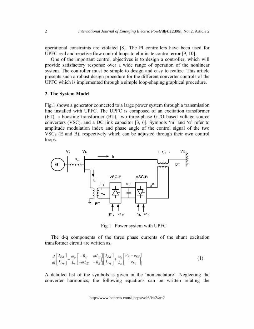
operational constraints are violated [8]. The PI controllers have been used for UPFC real and reactive flow control loops to eliminate control error [9, 10]. One of the important control objectives is to design a controller, which will provide satisfactory response over a wide range of operation of the nonlinear system. The controller must be simple to design and easy to realize. This article presents such a robust design procedure for the different converter controls of the UPFC which is implemented through a simple loop-shaping graphical procedure. 2. The System Model Fig.1 shows a generator connected to a large power system through a transmission line installed with UPFC. The UPFC is composed of an excitation transformer (ET), a boosting transformer (BT), two three-phase GTO based voltage source converters (VSC), and a DC link capacitor [3, 6]. Symbols ‘m’ and ‘α’ refer to amplitude modulation index and phase angle of the control signal of the two VSCs (E and B), respectively which can be adjusted through their own control loops.

Eα Bα

Fig.1 Power system with UPFC

The d-q components of the three phase currents of the shunt excitation transformer circuit are written as,

Ed Ed E EdE Eo o

Eq Eq EqE Es s

I I V eR LdI I eL Rdt L L

ωω ωω

−⎡ ⎤ ⎡ ⎤ ⎡ ⎤−⎡ ⎤= +⎢ ⎥ ⎢ ⎥ ⎢ ⎥⎢ ⎥ −− −⎢ ⎥ ⎢ ⎥ ⎢ ⎥⎣ ⎦⎣ ⎦ ⎣ ⎦ ⎣ ⎦

(1)

A detailed list of the symbols is given in the ‘nomenclature’. Neglecting the converter harmonics, the following equations can be written relating the

2 International Journal of Emerging Electric Power SystemsVol. 6 [2006], No. 2, Article 2

http://www.bepress.com/ijeeps/vol6/iss2/art2

amplitudes of the voltage vector components at the shunt converter AC-side terminals to the capacitor voltage (Vc) on the common DC link: cosEd E c Ee m V α= (2) sinEq E c Ee m V α= (3)

αE is the phase angle difference between the input converter AC voltage eE and the line voltage VE. The factor mE is the modulation index of the shunt converter. The instantaneous powers at the AC and DC terminals of the input and output converters are equal if the converters are assumed to be lossless. This gives two power balance equations in per unit, c i Ed Ed Eq EqV I e I e I= + (4) c o Bd Ld Bq LqV I e I e I= + (5) Since the net current to the capacitor is zero, for input current Ii and output Io the DC link circuit can be described by the equation as,

( )ci o

dVC I Idt

= + (6)

Similar to (2) and (3), the d-q components of the series injected voltage are, cosBd B c Be m V α= (7) sinBq B c Be m V α= (8)

Here, αB is the angle between eB and VE, and mB is the modulation index of the output converter. The transmission circuit equations including the series transformer of the UPFC can be expressed in d-q axes as,

Ld Ld E bd BdL Lo o

Lq Lq bq BqL LL L

I I V V eR LdI I V eL Rdt L L

ωω ωω

− −⎡ ⎤ ⎡ ⎤ ⎡ ⎤−⎡ ⎤= +⎢ ⎥ ⎢ ⎥ ⎢ ⎥⎢ ⎥ − −− −⎢ ⎥ ⎢ ⎥ ⎢ ⎥⎣ ⎦⎣ ⎦ ⎣ ⎦ ⎣ ⎦

(9)

In (9), IL represents the transmission line current; Vb and eB are the bus voltage and the series injected voltages, respectively. Recognizing that,

⎥⎦

⎤⎢⎣

⎡=⎥

⎦

⎤⎢⎣

⎡⎥⎦

⎤⎢⎣

⎡=⎥

⎦

⎤⎢⎣

⎡

Lq

Ld

oq

od

Eq

Ed

iq

id

II

II

II

II

; (10)



(4-5) and (7-8) substituted in (6) gives,

]coscossincos[1LqBBLdBBEqEEEdEE

c ImImImImCdt

dV αααα +++= (11)

The synchronous generator-exciter system is represented through a fourth order model as,

fdA

ttoA

Afd

dddqofddo

q

em

o

ET

VVTKE

ixxeET

e

DPPH

∆−−=∆

−−−=

−−=

=

1][

])([1

][21

'''

'

&

&

&

&

ωω

ωωδ

(12)

The expressions for electrical power output (Pe) and generator terminal voltage (Vt) are written in terms of the states as,

)](2)()([

])[(

'2'2'22

'''

LdEdqqLdEddLqEqqt

EqLdLqEdLqLdEqEddqLqqEqqe

IIeeIIxIIxV

IIIIIIIIxxIeIeP

+−++++=

+++−++= (13)

Substituting (13) in (12), and combining (1), (9), (11) and (12), the composite model of a synchronous generator UPFC system can be expressed through the 9th order dynamic relationship, ],[ uxfx =& (14) Here, the state vector x =[IEd IEq ILd ILq Vc δ ω eq

’ Efd]T and the control (u) comprises of [mE αE mB αB]. 3. Determination of the Operating States of UPFC While the steady state model of a single machine infinite bus system is relatively simple, the problem of UPFC control with operational and stability constraints does not have a simple solution. This is because UPFC makes the power-angle curve of a power system capable of two dimensional movement in the power-angle plane, and also because of the incorporation of operational constraints might



cause the power angle curves lose their continuity for steady state operation in the δ region of interest [8]. Determination of steady operating values generally involves iterative solution of nonlinear simultaneous equations so as to match the power balance constraints of the system including the converters. The controls can drive the operating values to new regimes even if the original system conditions are restored. Checks have to be made to verify whether the new equilibrium point satisfy all the steady state constraints. The following steps give a systematic search procedure for establishing the steady state operating conditions of the UPFC under the specified constraints:

1. For chosen system bus voltage magnitude Vb and input voltage VE (mE), calculate the transmission angle for a particular loading. Consider the controlled voltage VE to be the reference.

2. Calculate the transmission line current IL =(VE -Vb)/(rL+jxL) 3. Calculate the voltage across the booster transformer eB= (rB+jxB)IL ; where,

rB, xB are the resistance and reactance of the series transformer, respectively.

4. Calculate DC capacitor voltage Vc from the relation, ׀eB׀= mBVc 5. Find ׀eE׀ from the relationship, ׀eE׀= mEVc 6. Choose angle of eE with respect to VE . The angle is small. Calculate, IE = (VE - eE)/(rE+jxE) ; rE and xE are the resistance and reactance of the

exciting transformer. 7. Calculate the current supplied by the generator as, I=IL+IE 8. Calculate the generator terminal voltage, Vt = VE + jxtI; xt is the

transformer reactance connected to the generator bus. 9. Locate the quadrature (q) axis through the relationship, Eq= Vt + jxqI 10. Find d-q components of all the state and other required quantities. 11. Compute power output of the series (booster) converter PoB = eBdILd +

eBqILq 12. Compute the power output to the shunt (excitation) converter as, PoE =

eEdIEd + eEqIEq and compare with that in step 11. The values should be equal and of opposite sign.

13. If power balance is not achieved, change angle of eE by a small amount and go back to step 6.

15. When the algorithm converges, calculate αE and αB to satisfy the relationships,

eBd = ׀eB׀ cos αB, eBq =׀eB׀ sin αB, eEd = ׀eE׀ cos αE, eEq = ׀eE׀ cos αE; α ‘s are measured with respect to d-axis identified in step 9.



4. Robust UPFC Damping Controller Design The damping control problem for the nonlinear power system model is stated as: given the system represented by (14), design a controller whose output will stabilize the system following a perturbation in the system. Since there is no general method of designing a stabilizing controller for the nonlinear system, one way would be to perform the control design for a linearized system; the linearization being carried out around a nominal operating condition. If the controller designed is ‘robust’ enough to perform well for the other operating conditions in the vicinity, the design objectives are met. The linearized system of state equations are written as,

CXY

BuAXX=

+=& (15)

In (15) the state and output variables (X,Y) are perturbed quantities around the nominal values. The system matrices (A,B,C) depend on the operating point selected. The changes in operation of the nonlinear system (14) can be considered as changes in the elements of the system matrices. These perturbations are modeled as uncertainties and robust design procedure is applied to the perturbed linear systems. The design is carried out using the minimization of performance measures expressed in terms of H∞ norms. A graphical construction procedure called ‘loop-shaping’ has been employed for the robust control design. A brief theory of the uncertainty model, the robust stability criterion, and the graphical design technique are presented along with an algorithm for the design steps.

Suppose that the linearized plant having a nominal transfer function P belongs to a bounded set of transfer functions P. Consider that the perturbed transfer function resulting from the variations in operating conditions can be expressed in the form,

PWP )1( 2

~

Ω+= ; P=C[sI-A]-1B (16) Here, W2 is a fixed stable transfer function, also called the weight, and Ω is a variable transfer function satisfying

∝Ω < 1. The infinity norm (∝-norm) of a

function is the least upper bound of its absolute value, also written as

∝Ω = )(sup ω

ωjΩ , and is the largest value of gain on a Bode magnitude plot. In

the multiplicative uncertainty model (16), ΩW2 is the normalized plant perturbation away from unity. If

∝Ω < 1, then,



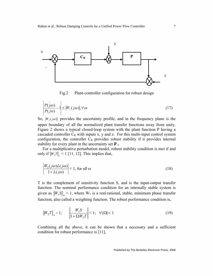
Fig.2 Plant-controller configuration for robust design

ωωω∀≤− ,)(1

)()(

2

~

jWjwPjP

(17)

So, )(2 ωjW provides the uncertainty profile, and in the frequency plane is the upper boundary of all the normalized plant transfer functions away from unity. Figure 2 shows a typical closed-loop system with the plant function P having a cascaded controller CR with inputs x, y and z. For this multi-input control system configuration, the controller CR provides robust stability if it provides internal stability for every plant in the uncertainty set P. For a multiplicative perturbation model, robust stability condition is met if and only if

∝TW2 < 1 [11, 12]. This implies that,

)(1

)()(2

ωωω

jLjLjW

+< 1, for all ω (18)

T is the complement of sensitivity function S, and is the input-output transfer function. The nominal performance condition for an internally stable system is given as

∝SW1 < 1, where W1 is a real-rational, stable, minimum phase transfer

function, also called a weighting function. The robust performance condition is,

∝

TW2 < 1; TW

SW

2

1

1 Ω+< 1; ∀||Ω||< 1 (19)

Combining all the above, it can be shown that a necessary and a sufficient condition for robust performance is [11],

CR P x

z

-

y



∝

+ TWSW 21 < 1 (20) Loop shaping is a graphical procedure to design a proper controller CR

satisfying the robust stability and performance criteria given above. The basic idea of the method is to construct the loop transfer function L to satisfy the robust performance criterion approximately, and then to obtain the controller from the relationship CR =L/P. Internal stability of the plants and properness of CR constitute the constraints of the method. Condition on L is such that PCR should not have any pole zero cancellation.

A necessary condition for robustness is that either or both 21 , WW must be less than one [13]. If we select a monotonically decreasing W1 satisfying the other constraints on it, it can be shown that at low frequency the open-loop transfer function L should satisfy,

2

1

1 WW

L−

> (21)

while, for high frequency,

22

1 11WW

WL ≈

−< (22)

At high frequency L should roll-off at least as quickly as P does. This ensures

properness of CR. The general features of the open loop transfer function is that the gain at low frequency should be large enough for the steady state error considerations, and L should not drop-off too quickly near the crossover frequency resulting in internal instability. The algorithm to generate a robust control function CR involves the following steps:

1. From the linearized system find the nominal plant transfer function P. 2. Obtain the db-magnitude plot for the nominal as well as perturbed plant

transfer functions. 3. Construct W2 satisfying constraint (17). 4. Select W1 as a monotonically decreasing, real, rational and stable function. 5. Choose L such that it satisfies conditions (21) and (22). The transition at

crossover frequency should not be at slope steeper than –20db/decade. Nominal internal stability is achieved if, on a Nyquist plot of L, the angle of L at crossover is greater than 1800.



6. Check for the nominal performance criterion ∝

SW1 < 1, and robust performance measure given by (20).

7. Construct the controller function from the relation CR =L/P 8. Test for internal stability by direct simulation of the closed loop transfer

function for pre-selected disturbance or input. 9. Repeat steps 5 through 8 until satisfactory L and CR are obtained.

5. Implementation of the Controller Designs The four control inputs which can be modulated in order to produce damping torque are [mE αE mB αB], as identified in (14). However, the UPFC bus is assumed to be a voltage controlled bus, and so the magnitude of this voltage VE (Fig. 1) cannot be modulated. In the following, robust designs for the three other controllers mB, αE and αB are implemented independently followed by their coordinated applications. 5.1 The Robust Series Converter Voltage Magnitude (mB) Control In the collapsed plant-controller configuration of Fig.2, P is constructed such that the modulation index of the series converter voltage magnitude (mB) is the input to the plant and the generator speed deviation (∆ω) is the output. The power output at the nominal operating point is considered as 1.01 pu, at 0.94 pf lag. The parameters and other operating values for the UPFC system are given in the Appendix. The nominal plant transfer is obtained as,

)p......(s..........).........p)(sp(s)z..(s).........z)(sz135.539(sP

921

721++++++

= (23)

The zeroes and poles of the system, respectively are [0,-3098.4,-19.58, -27±j364.15, -0.22±j0.743], [-19.72,-28.08 ± j2790.3, -9.4 ± j377.506, -0.212 ±j 4.15, -0.25 ± j0.75]. Off-nominal power output in the range of 0.3-1.4 pu and power factor of up to 0.8 lag/lead which gave steady state stable situations were considered in the robust design. The quantity 1)(/)(~ −ωω jPjP nom is constructed

for each perturbed plant )(~ ωjP and the upper envelope in the frequency plane is fitted to the function,

166.1

64.02.348.0)( 2

2

2 ++++

=sssssW (24)



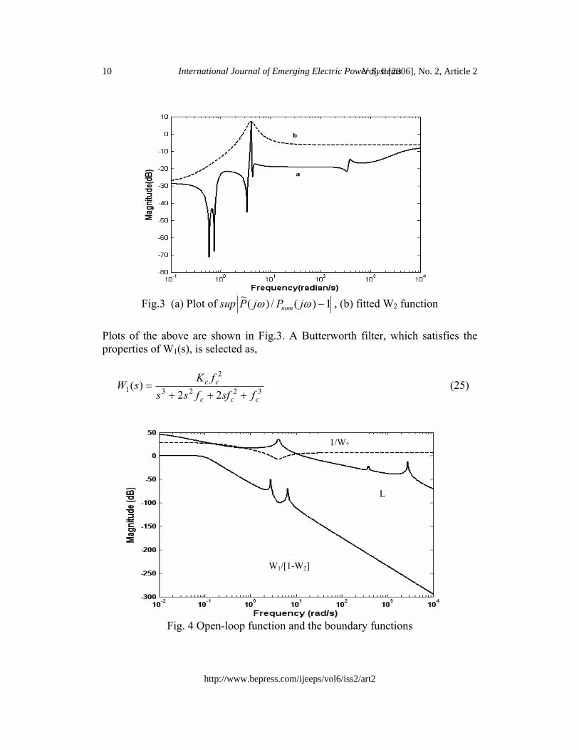
Fig.3 (a) Plot of sup 1)(/)(~ −ωω jPjP nom , (b) fitted W2 function

Plots of the above are shown in Fig.3. A Butterworth filter, which satisfies the properties of W1(s), is selected as,

3223

2

1 22)(

ccc

cc

fsffssfK

sW+++

= (25)

Fig. 4 Open-loop function and the boundary functions

1/W2

L

W1/[1-W2]



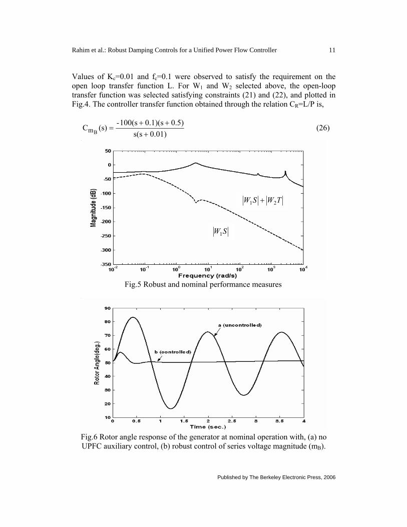
Values of Kc=0.01 and fc=0.1 were observed to satisfy the requirement on the open loop transfer function L. For W1 and W2 selected above, the open-loop transfer function was selected satisfying constraints (21) and (22), and plotted in Fig.4. The controller transfer function obtained through the relation CR=L/P is,

0.01)s(s

.5)00.1)(s100(s-(s)CBm +

++= (26)

Fig.5 Robust and nominal performance measures

Fig.6 Rotor angle response of the generator at nominal operation with, (a) no UPFC auxiliary control, (b) robust control of series voltage magnitude (mB).

TWSW 21 +

SW1



The robust and nominal performance measures are shown in Fig.5. It can be observed that the nominal performance measure is very small relative to 0 db. The robust stability measure is marginally violated at the corner frequency. This is for a worst-case design in the absence of damping term in the electromechanical swing equation. While selecting the open-loop transfer function, the internal stability of the plant in addition to the design criterion (19)-(22) had to be checked. A disturbance of 50% input torque pulse for 0.1 second on the generator shaft was simulated for this purpose. The rotor angle variations of the generator for the nominal operating point with and without the robust controller are plotted in Fig. 6. As can be observed, the robust mB controller provides extremely good damping to the rotor oscillations.

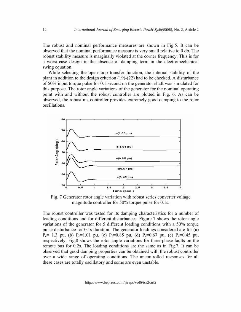
Fig. 7 Generator rotor angle variation with robust series converter voltage

magnitude controller for 50% torque pulse for 0.1s. The robust controller was tested for its damping characteristics for a number of loading conditions and for different disturbances. Figure 7 shows the rotor angle variations of the generator for 5 different loading conditions with a 50% torque pulse disturbance for 0.1s duration. The generator loadings considered are for (a) Pe= 1.3 pu, (b) Pe=1.01 pu, (c) Pe=0.85 pu, (d) Pe=0.67 pu, (e) Pe=0.45 pu, respectively. Fig.8 shows the rotor angle variations for three-phase faults on the remote bus for 0.2s. The loading conditions are the same as in Fig.7. It can be observed that good damping properties can be obtained with the robust controller over a wide range of operating conditions. The uncontrolled responses for all these cases are totally oscillatory and some are even unstable.



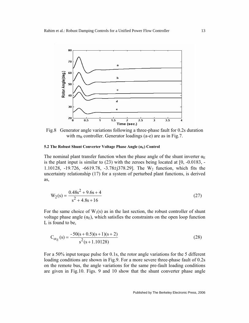
Fig.8 Generator angle variations following a three-phase fault for 0.2s duration

with mB controller. Generator loadings (a-e) are as in Fig.7. 5.2 The Robust Shunt Converter Voltage Phase Angle (αE) Control The nominal plant transfer function when the phase angle of the shunt inverter αE is the plant input is similar to (23) with the zeroes being located at [0, -0.0183, -1.10128, -19.726, -6619.78, -3.78±j378.29]. The W2 function, which fits the uncertainty relationship (17) for a system of perturbed plant functions, is derived as,

16s8.4s

4s6.9s48.0)s(W 2

22

++

++= (27)

For the same choice of W1(s) as in the last section, the robust controller of shunt voltage phase angle (αE), which satisfies the constraints on the open loop function L is found to be,

1.10128)(ss

2)1)(s0.5)(s50(s-(s)C 2E +

+++=α (28)

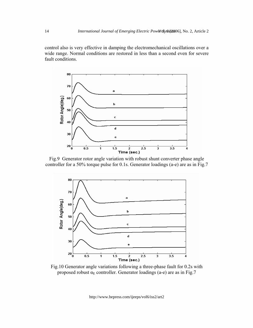
For a 50% input torque pulse for 0.1s, the rotor angle variations for the 5 different loading conditions are shown in Fig.9. For a more severe three-phase fault of 0.2s on the remote bus, the angle variations for the same pre-fault loading conditions are given in Fig.10. Figs. 9 and 10 show that the shunt converter phase angle



control also is very effective in damping the electromechanical oscillations over a wide range. Normal conditions are restored in less than a second even for severe fault conditions.

Fig.9 Generator rotor angle variation with robust shunt converter phase angle

controller for a 50% torque pulse for 0.1s. Generator loadings (a-e) are as in Fig.7

Fig.10 Generator angle variations following a three-phase fault for 0.2s with

proposed robust αE controller. Generator loadings (a-e) are as in Fig.7



5.3 The Robust Series Converter Phase angle (αB) Control The nominal plant function with the phase angle of the series converter injected voltage (αB) as the input to the plant has the zeroes located at [0, 1416.234, -20.4812, -0.617, 0.0894, -31.876±j397.995] for the same nominal operating conditions. The W2 function obtained is,

)1s0005.0)(1s3.0(

)1s004.0)(1s25.0(85.0)s(W2 ++++

= (29)

While it was possible to find controller functions which gave some damping

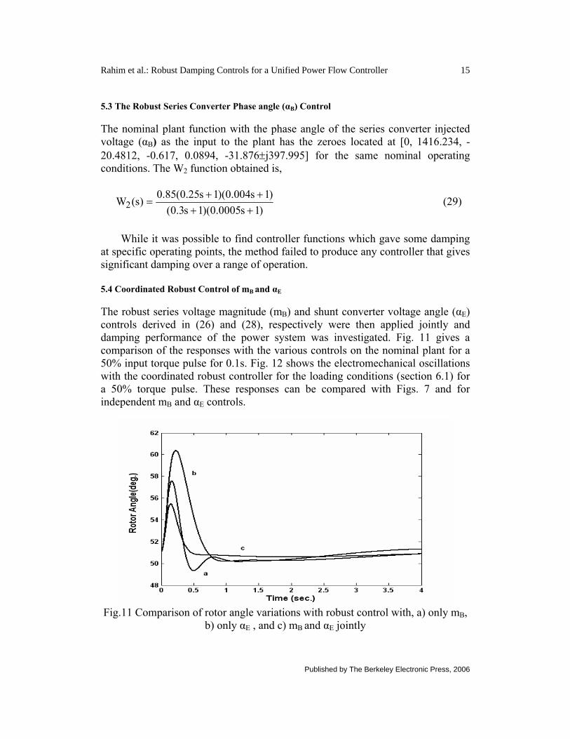
at specific operating points, the method failed to produce any controller that gives significant damping over a range of operation. 5.4 Coordinated Robust Control of mB and αE The robust series voltage magnitude (mB) and shunt converter voltage angle (αE) controls derived in (26) and (28), respectively were then applied jointly and damping performance of the power system was investigated. Fig. 11 gives a comparison of the responses with the various controls on the nominal plant for a 50% input torque pulse for 0.1s. Fig. 12 shows the electromechanical oscillations with the coordinated robust controller for the loading conditions (section 6.1) for a 50% torque pulse. These responses can be compared with Figs. 7 and for independent mB and αE controls.

Fig.11 Comparison of rotor angle variations with robust control with, a) only mB,

b) only αE , and c) mB and αE jointly



0 0.5 1 1.5 2 2.5 3 3.5 420

25

30

35

40

45

50

55

60

65

70

a

b

c

d

e

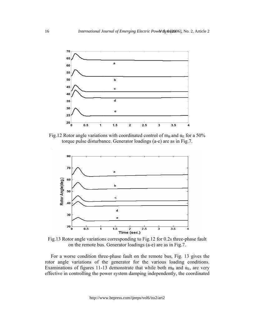
Fig.12 Rotor angle variations with coordinated control of mB and αE for a 50%

torque pulse disturbance. Generator loadings (a-e) are as in Fig.7.

Fig.13 Rotor angle variations corresponding to Fig.12 for 0.2s three-phase fault

on the remote bus. Generator loadings (a-e) are as in Fig.7. For a worse condition three-phase fault on the remote bus, Fig. 13 gives the rotor angle variations of the generator for the various loading conditions. Examinations of figures 11-13 demonstrate that while both mB and αE, are very effective in controlling the power system damping independently, the coordinated



application of these provide the best response. If from operational considerations only one control is to be employed, then the robust mB should be selected. 6. Evaluation of the Robust Strategy The damping properties of the proposed coordinated robust controller were compared with a conventional PI controller. The PI controllers have been used for UPFC real and reactive flow control loops to eliminate control error [8, 14, 15]. The PI or PID controllers are normally installed in the feedback path. An additional washout is included in cascade with the controller to eliminate any unwanted signal in the steady state. The controller function in the feedback loop is written as,

⎥⎦

⎤⎢⎣

⎡+

+=w

wIP sT

sTs

KKsH1

][)( (30)

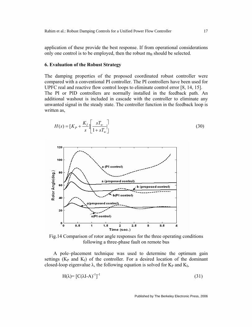
Fig.14 Comparison of rotor angle responses for the three operating conditions

following a three-phase fault on remote bus A pole–placement technique was used to determine the optimum gain

settings (KP and KI) of the controller. For a desired location of the dominant closed-loop eigenvalue λ, the following equation is solved for KP and KI,

H(λ)= [C(λI-A)-1]-1 (31)



H(λ) is obtained from (30) for the desired λ . The dominant eigenvalues of the closed loop system in the present study were selected to be at -1.25 ±j3.973, corresponding to a damping ratio of approximately 0.3. The values for KP and KI for mB control were found to be -38.932 and -69.05, while they are –10.7023 and –10.30947, respectively for αE.

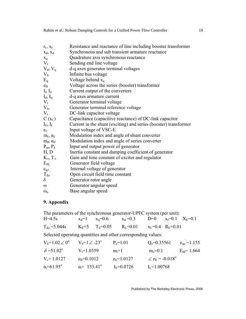
A comparison of the responses with the PI control and proposed robust strategies for a three-phase fault disturbance are shown in Fig. 14. The three loading conditions are a)1.3 pu, b)1.01 pu, and c)0.45 pu. While the response with the PI control is reasonably good at the nominal point (1.01 pu) which it is designed for, it starts to deteriorate at operating points away from the nominal. For points relatively far away, the controller may even lead to unstable performance. This is demonstrated by response in the figure by curve ‘a(PI)’ corresponding to case a. The response with the proposed robust controller can be observed to be much superior. 7. Conclusions Power system damping improvement through various UPFC controls has been investigated. Fixed parameter robust damping controllers have been designed for shunt and series converters using a relatively simple graphical loop-shaping technique satisfying H-∞ based robust stability and performance criteria. The robust design includes a detailed nonlinear model of the UPFC-generator system. The controllers designed were tested for a number of disturbance conditions including symmetrical three-phase faults. Series converter voltage magnitude and shunt converter phase angle were observed to provide very good damping independently, the series voltage magnitude control being superior. Simultaneous application of these two controls, however, was found to provide the best performance. Comparison of the proposed damping control strategies with PI controllers having optimized gain settings clearly exhibits the robustness of the proposed controllers. The graphical loop-shaping method can be routinely extended to a multi-machine power system. However, placing the open-loop poles of a very large order system manually is, generally, inconvenient. In order to overcome the dimensional complexity, the authors are looking into the possibility of embedding a search based optimization procedure in the loop-shaping method which will start by pre-selecting the structure of the controller. 8. Nomenclature d-q Direct and quadrature axes of generator rE, xE Resistance and reactance of exciting transformer



rL, xL Resistance and reactance of line including booster transformer xd, xd

’ Synchronous and sub transient armature reactance xq Quadrature axis synchronous reactance VE Sending end line voltage Vd, Vq d-q axes generator terminal voltages Vb Infinite bus voltage Eq Voltage behind xq eB Voltage across the series (booster) transformer Ii, Io Current output of the converters Id, Iq d-q axes armature current Vt Generator terminal voltage Vto Generator terminal reference voltage Vc DC-link capacitor voltage C (xC) Capacitance (capacitive reactance) of DC-link capacitor IE, IL Current in the shunt (exciting) and series (booster) transformer eE Input voltage of VSC-E mE, αE Modulation index and angle of shunt converter mB, αB Modulation index and angle of series converter Pm, Pe Input and output power of generator H, D Inertia constant and damping coefficient of generator KA, TA Gain and time constant of exciter and regulator Efd Generator field voltage eqo

’ Internal voltage of generator Tdo

’ Open circuit field time constant δ Generator rotor angle ω Generator angular speed ωo Base angular speed 9. Appendix

The parameters of the synchronous generator-UPFC system (per unit): H=4.5s xd=1 xq=0.6 xd

’=0.3 D=0 xt=0.1 XE=0.1

Tdo’=5.044s KE=5 TE=0.05 RL=0.01 xL=0.4 RE=0.01

Selected operating quantities and other corresponding values:

VE=1.02∠ 0o Vb=1∠ -23o Pe=1.01 Qe=0.35561 eqo’=1.155

δ =51.02o Vt=1.0359 mi=1 mo=0.1 Efd= 1.664

Vc= 1.0127 eB=0.1012 eE=1.0127 ∠ eE = -0.018o

αi=61.95o αi= 133.41o IE=0.0726 IL=1.00768



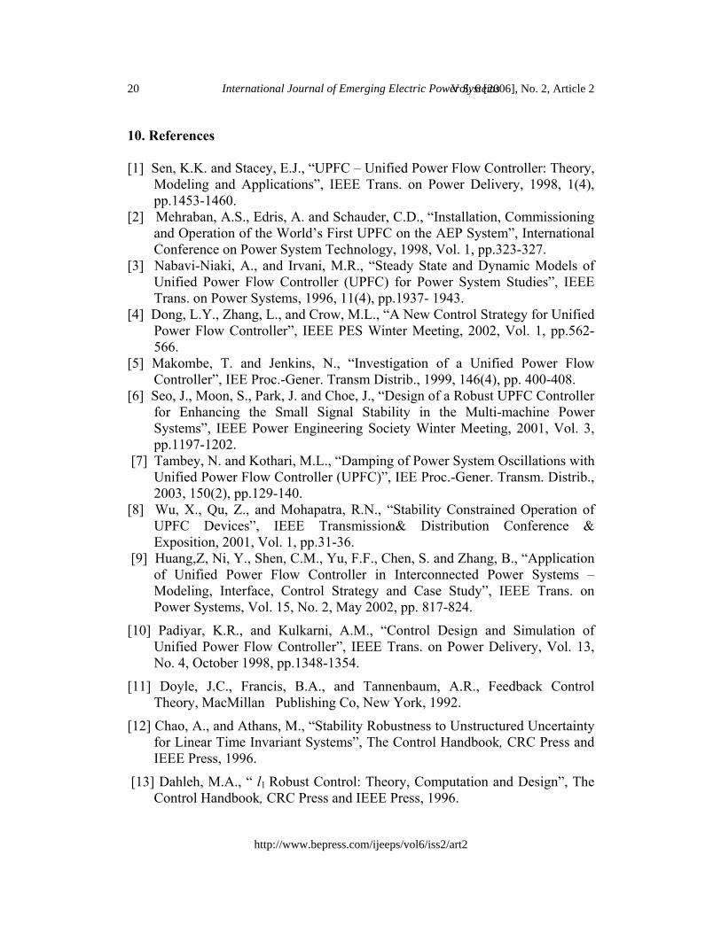
10. References [1] Sen, K.K. and Stacey, E.J., “UPFC – Unified Power Flow Controller: Theory,

Modeling and Applications”, IEEE Trans. on Power Delivery, 1998, 1(4), pp.1453-1460.

[2] Mehraban, A.S., Edris, A. and Schauder, C.D., “Installation, Commissioning and Operation of the World’s First UPFC on the AEP System”, International Conference on Power System Technology, 1998, Vol. 1, pp.323-327.

[3] Nabavi-Niaki, A., and Irvani, M.R., “Steady State and Dynamic Models of Unified Power Flow Controller (UPFC) for Power System Studies”, IEEE Trans. on Power Systems, 1996, 11(4), pp.1937- 1943.

[4] Dong, L.Y., Zhang, L., and Crow, M.L., “A New Control Strategy for Unified Power Flow Controller”, IEEE PES Winter Meeting, 2002, Vol. 1, pp.562-566.

[5] Makombe, T. and Jenkins, N., “Investigation of a Unified Power Flow Controller”, IEE Proc.-Gener. Transm Distrib., 1999, 146(4), pp. 400-408.

[6] Seo, J., Moon, S., Park, J. and Choe, J., “Design of a Robust UPFC Controller for Enhancing the Small Signal Stability in the Multi-machine Power Systems”, IEEE Power Engineering Society Winter Meeting, 2001, Vol. 3, pp.1197-1202.

[7] Tambey, N. and Kothari, M.L., “Damping of Power System Oscillations with Unified Power Flow Controller (UPFC)”, IEE Proc.-Gener. Transm. Distrib., 2003, 150(2), pp.129-140.

[8] Wu, X., Qu, Z., and Mohapatra, R.N., “Stability Constrained Operation of UPFC Devices”, IEEE Transmission& Distribution Conference & Exposition, 2001, Vol. 1, pp.31-36.

[9] Huang,Z, Ni, Y., Shen, C.M., Yu, F.F., Chen, S. and Zhang, B., “Application of Unified Power Flow Controller in Interconnected Power Systems – Modeling, Interface, Control Strategy and Case Study”, IEEE Trans. on Power Systems, Vol. 15, No. 2, May 2002, pp. 817-824.

[10] Padiyar, K.R., and Kulkarni, A.M., “Control Design and Simulation of Unified Power Flow Controller”, IEEE Trans. on Power Delivery, Vol. 13, No. 4, October 1998, pp.1348-1354.

[11] Doyle, J.C., Francis, B.A., and Tannenbaum, A.R., Feedback Control Theory, MacMillan Publishing Co, New York, 1992.

[12] Chao, A., and Athans, M., “Stability Robustness to Unstructured Uncertainty for Linear Time Invariant Systems”, The Control Handbook, CRC Press and IEEE Press, 1996.

[13] Dahleh, M.A., “ l1 Robust Control: Theory, Computation and Design”, The Control Handbook, CRC Press and IEEE Press, 1996.



[14] Z.Huang, Y. Ni, C.M.Shen, F.F. Yu, S.Chen and B.Zhang, “Application of Unified Power Flow Controller in Interconnected Power Systems – Modeling, Interface, Control Strategy and Case Study”, IEEE trans. on Power Systems, Vol. 15, No. 2, May 2002, pp. 817-824.

[15] K.R.Padiyar and A.M.Kulkarni, “Control Design and Simulation of Unified Power Flow Controller”, IEEE Trans. on Power Delivery, Vol. 13, No. 4, October 1998, pp.1348-1354.



Date post:	28-Jun-2018
Category:	Documents
Upload:	phamhanh
View:	215 times
Download:	0 times

International Journal of Emerging Electric Power...

Documents