International Journal of Multiphase Flow 43 (2012) 85–100

Contents lists available at SciVerse ScienceDirect

International Journal of Multiphase Flow

journal homepage: www.elsevier .com/ locate / i jmulflow

CFD modeling for pipeline flow of fine particles at high concentration

D.R. Kaushal a,⇑, T. Thinglas a, Yuji Tomita b, Shigeru Kuchii c, Hiroshi Tsukamoto c

a Department of Civil Engineering, IIT Delhi, Hauz Khas, New Delhi 110 016, Indiab Kyushu Institute of Technology, 1-1 Sensui cho, Tobata, Kitakyushu 804-8550, Japanc Kitakyushu National College of Technology, 5-20-1 Shii, Kokura-minami, Kitakyushu 802-0985, Japan

a r t i c l e i n f o a b s t r a c t

Article history:Received 5 May 2011Received in revised form 4 March 2012Accepted 8 March 2012Available online 17 March 2012

Keywords:3D CFD modelingEulerian modelMixture modelConcentration distributionSlurry pipelinePressure drop

0301-9322/$ - see front matter � 2012 Elsevier Ltd. Ahttp://dx.doi.org/10.1016/j.ijmultiphaseflow.2012.03.0

⇑ Corresponding author. Tel.: +91 9818280867; faxE-mail address: kaushal@civil.iitd.ac.in (D.R. Kaush

Pipeline slurry flow of mono-dispersed fine particles at high concentration is numerically simulated usingMixture and Eulerian two-phase models. Both the models are part of the CFD software package FLUENT. Ahexagonal shape and cooper type non-uniform three-dimensional grid is chosen to discretize the entirecomputational domain, and a control volume finite difference method was used to solve the governingequations. The modeling results are compared with the authors’ experimental data collected in54.9 mm diameter horizontal pipe for concentration profiles at central vertical plane using c-ray densi-tometer and pressure drop along the pipeline using differential pressure transducers. Experiments areperformed on glass beads with mean diameter of 125 lm for flow velocity up to 5 m/s and four overallconcentrations up to 50% (namely, 0%, 30%, 40% and 50%) by volume for each velocity. The modelingresults by both the models for pressure drop in the flow of water are found to be in good agreement withexperimental data. For flow of slurry, Mixture model fails to predict pressure drops correctly. The amountof error increases rapidly with the slurry concentration. However, Eulerian model gives fairly accuratepredictions for both the pressure drop and concentration profiles at all efflux concentrations and flowvelocities. Velocity and slip-velocity distributions, that have never been measured experimentally at suchhigher concentrations, predicted by Eulerian model are presented for the concentration and velocityranges covered in this study. Slip velocity between fluid and solids dragged most of the particles in thecentral core of pipeline, resulting point of maximum concentration to occur away from the pipe bottom.

� 2012 Elsevier Ltd. All rights reserved.

1. Introduction

Conveyance of solids through pipelines on large scale has nowcome to be accepted as a viable alternative to the conventionalmodes of transportation. Pipes are very commonly used for longdistance transportation and, at present in the world, there aremany pipelines transporting different solid materials such as coal,fly ash, lime stone, zinc tailings, rock phosphate gilsonite, copperconcentrate and iron concentrate. In difficult terrains, such asystem of transportation is found to be techno economically moresuitable as compared to conventional modes like railways, road-ways and conveyors. A study of existing slurry pipe line systemsshows that they broaden the economic reach of mineral depositswhich could be utilized, since such a system could be used totransport materials from remotest areas which are otherwise notaccessible to conventional modes of transport. In any practicalsituation, the solids being transported are multisized and their sizemay span three orders of magnitude.

The flow of slurry is very complex. It has been theendeavour of researchers around the world to develop accurate

ll rights reserved.05

: +91 11 26581117.al).

models for concentration distribution in slurry pipeline. Thesemodels may be used to determine the parameters of directimportance (mixture and solid flow rates and pressure drop)and the secondary effects such as wall abrasion and particledegradation.

The advection–diffusion (AD) model has been extensively usedto predict the variation with depth of the particle concentrationdue to its simplicity (Kaushal and Tomita, 2002). However, ADmodel is unable to predict the concentration profiles with pointsof maximum concentration away from the pipe bottom (Kaushaland Tomita, 2007). The reasons for such drawbacks in AD modelare described later, in the article 5.5 of this paper.

CFD based approach for investigating the variety of multiphasefluid flow problems in closed conduits and open channel are beingincreasingly used. One advantage with CFD-based approach is thatthree dimensional solid–liquid two phase flow problems under awide range of flow conditions and sediment characteristics maybe evaluated rapidly, which is almost impossible experimentally.Thinglas and Kaushal (2008a, 2008b) have recently performedthree dimensional CFD modeling for optimization of invert trapconfiguration to be used in sewer solid management. However,the use of such methodology for evaluating flow characteristicsin slurry pipelines is limited.

86 D.R. Kaushal et al. / International Journal of Multiphase Flow 43 (2012) 85–100

Ling et al. (2003) proposed a simplified three dimensional alge-braic slip mixture (ASM) model to obtain the numerical solution insand–water slurry flow. In order for the study to obtain the precisenumerical solution in fully developed turbulent flow, the RNG k–eturbulent model was used with the ASM model. An unstructured(block-structured) non-uniform grid was chosen to discretize theentire computational domain, and a control volume finite differ-ence method was used to solve the governing equations. The meanpressure gradients from the numerical solutions were comparedwith the authors’ experimental data and that in the open literatureup to an average volumetric concentration of 20%. The solutionswere found to be in good agreement when the slurry velocity ishigher than the corresponding critical deposition velocity. How-ever, as mentioned in FLUENT manual (2005), Mixture model usedby Ling et al. (2003) holds good only for moderate concentrations.For the flow of high concentration slurries, the same manual rec-ommends use of Eulerian multiphase model.

Kaushal and Tomita (2007) repeated experimental study forconcentration distributions in slurry pipeline conducted by Kau-shal et al. (2005) by using c-ray densitometer. Their measurementsshow that, for finer particles, point of maximum concentrations arenear the pipe bottom and for coarser particles, maximum pointsare relatively away from the pipe bottom with decrease in shiftas flow velocity increases. Pressure gradient profiles of equivalentfluid for finer particles were found to resemble with water data ex-cept for 50% concentration, however, more skewed pressure gradi-ent profiles of equivalent fluid were found for coarser particles.Experimental results indicate absence of near-wall lift for finerparticles due to submergence of particles in the lowest layer intothe viscous sublayer and presence of considerable near-wall liftfor coarser particles due to impact of viscous-turbulent interfaceon the bottom most layer of particles and increased particle–parti-cle interactions. It is observed that near-wall lift decreases with in-crease in flow velocity. Kaushal and Tomita (2007) also concludedthat the near-wall lift observed in case of coarser particles is notassociated with the Magnus effect, the Saffman force or Campbellet al. (2004) lift-like interaction force, and not yet modeledmathematically.

In the present study, three-dimensional concentration distri-butions, pressure drops and velocity distributions are modeledusing Mixture and Eulerian models in 54.9 mm diameter horizon-tal pipe on glass beads with specific gravity of 2.47, mean diam-eter (d50) of 125 lm and geometric standard deviation of 1.15, forflow velocity up to 5 m/s and overall concentration up to 50% byvolume for each velocity. The computations are done consideringparticles as mono-dispersed. Three-dimensional modeling resultsfor concentration distribution and pressure drops are comparedwith the experimental data.

2. Mathematical model

The use of a specific multiphase model (the discrete phase, mix-ture, Eulerian model) to characterize momentum transfer dependson the volume fraction of solid particles and on the fulfillment ofthe requirements which enable the selection of a given model. Inpractice, slurry flow through pipeline is not a dilute system, there-fore the discrete phase model cannot be used to simulate its flow,but both the Mixture model and the Eulerian model are appropri-ate in this case. Further, out of two versions of Eulerian model,granular version will be appropriate in the present case. The reasonfor choosing the granular in favour of the simpler non-granularmulti-fluid model is that the non-granular model does not includemodels for taking friction and collisions between particles into ac-count which is believed to be of importance in the slurry flow. Thenon-granular model also lack possibilities to set a maximum pack-

ing limit which makes it less suitable for modeling flows with par-ticulate secondary phase in the present case. Lun et al. (1984) andGidaspow et al. (1992) proposed such a model for gas–solid flows.Slurry flow may be considered as gas–solid (pneumatic) flow byreplacing the gas phase by water and maximum packing concen-tration by static settled concentration. Furthermore, few forces act-ing on solid phase may be prominent in case of slurry flow, whichmay be neglected in case of pneumatic flow and vice versa. In thepresent study slurry pipeline is modeled using granular-Eulerianand Mixture models as described below:

2.1. Eulerian model

Eulerian model assumes that the slurry flow consists of solid ‘‘s’’and fluid ‘‘f’’ phases, which are separate, yet they form interpene-trating continua, so that af + as = 1.0, where af and as are the volu-metric concentrations of fluid and solid phase, respectively. Thelaws for the conservation of mass and momentum are satisfiedby each phase individually. Coupling is achieved by pressure andinterphasial exchange coefficients.

The forces acting on a single particle in the fluid:

1. Static pressure gradient, rP.2. Solid pressure gradient or the inertial force due to particle

interactions, rPs.3. Drag force caused by the velocity differences between two

phases, Ksf ð~ts �~tf Þ, where, Ksf is the inter-phase drag coeffi-cient, ~ts and ~tf are velocity of solid and fluid phase,respectively.

4. Viscous forces, r � ��sf , where, ��sf is the stress tensor for fluid.5. Body forces, q~g, where, q is the density and g is acceleration

due to gravity.6. Virtual mass force, Cvmasqf ð~tf � r~tf �~ts � r~tsÞ, where, Cvm is

the coefficient of virtual mass force and is taken as 0.5 in thepresent study.

7. Lift force, CLasqf ð~tf �~tsÞ � ðr �~tf Þwhere, CL is the lift coef-ficient taken as 0.5 in the present study as such a value issuggested in literature for glass beads.

2.1.1. Governing equations2.1.1.1. Continuity equation.

r � ðatqt~ttÞ ¼ 0 ð1Þ

where, t is either s or f.

2.1.1.2. Momentum equations. For fluid phase:

r � ðaf qf~tf~tf Þ ¼ �afrP þr � ��sf þ af qf~g þ Ksf ð~ts �~tf Þþ Cvmaf qf ð~ts � r~ts �~tf � r~tf Þþ CLasqf ð~tf �~tsÞ � ðr �~tf Þ ð2Þ

For solid phase:

r � ðasqs~ts~tsÞ ¼ �asrP �rPs þr �~s¼s þ asqf~g þ Kfsð~tf �~tsÞþ Cvmasqf ð~tf � r~tf �~ts � r~tsÞþ CLasqf ð~ts �~tf Þ � ðr �~tf Þ ð3Þ

where ��ss and ��sf are the stress tensors for solid and fluid, respec-tively, which are expressed as

��ss ¼ aslsðr~ts þr~ttrs Þ þ asðks �

23lsÞr �~ts

��I ð4Þ

and

��sf ¼ af lf ðr~tf þr~ttrf Þ ð5Þ

D.R. Kaushal et al. / International Journal of Multiphase Flow 43 (2012) 85–100 87

with superscript ‘tr’ over velocity vector indicating transpose. ��I isthe identity tensor. ks is the bulk viscosity of the solids as given by:

ks ¼43asqsdsgo;ss 1þ essð Þ Hs

p

� �12

ð6Þ

ds is the particle diameter put as 125 lm. go,ss is the radial distribu-tion function, which is interpreted as the probability of particletouching another particle:

go;ss ¼ 1� as

as;max

� �13

" #�1

ð7Þ

as,max is the static settled concentration measured experimentallyby Kaushal and Tomita (2007) as 0.63 for glass beads used in thepresent study. Hs is the granular temperature, which is proportionalto the kinetic energy of the fluctuating particle motion and is mod-eled as described in Section 2.1.4. ess is the restitution coefficient,taken as 0.9 for glass beads particles. lf is the shear viscosity offluid. ls is the shear viscosity of solids defined as

ls ¼ ls;col þ ls;kin þ ls;fr ð8Þ

where ls,col, ls,fr and ls,kin are collisional, frictional and kinetic vis-cosity are calculated using following expressions:

ls;col ¼45asqsdsgo;ssð1þ essÞ

Hs

p

� �12

ð9Þ

ls;fr ¼Ps sin /

2ffiffiffiffiffiffiI2Dp ð10Þ

and

ls;kin ¼asdsqs

ffiffiffiffiffiffiffiffiffiffiHspp

6ð3� essÞ1þ 2

5ð1þ essÞð3ess � 1Þasgo;ss

� �ð11Þ

I2D is the second invariant of the deviatoric strain rate tensor for so-lid phase. Ps is the solid pressure as given by:

Ps ¼ asqsHs þ 2qsð1þ essÞa2s go;ssHs ð12Þ

u is the internal friction angle taken as 30� in the present computa-tions. Ksf(=Kfs) is the interphasial momentum exchange coefficientgiven by

Ksf ¼ Kfs ¼34

asaf qf

V2r;sds

CDRes

Vr;s

� �j~ts �~tf j ð13Þ

CD is the drag coefficient given by:

CD ¼ 0:63þ 4:8Res

Vr;s

� ��12

" #2

ð14Þ

Res is the relative Reynolds number between phases ‘f’ and ‘s’given by

Res ¼qf dsj~ts �~tf j

lfð15Þ

Vr,s is the terminal velocity correlation for solid phase given by:

Vr;s ¼ 0:5 A� 0:06Res þffiffiffiffiffiffiffiffiffiffiffiffiffiffiffiffiffiffiffiffiffiffiffiffiffiffiffiffiffiffiffiffiffiffiffiffiffiffiffiffiffiffiffiffiffiffiffiffiffiffiffiffiffiffiffiffiffiffiffiffiffiffiffiffiffiffiffiffiffiffiffiffiffiffið0:06ResÞ2 þ 0:12Resð2B� AÞ þ A2

q� �ð16Þ

with

A ¼ a4:14f ; B ¼ 0:8a1:28

f for af 6 0:85; ð17Þ

and

A ¼ a4:14f ; B ¼ a2:65

f for af > 0:85: ð18Þ

2.1.2. Turbulence closure for the fluid phasePredictions for turbulent quantities for the fluid phase are ob-

tained using standard k–e model (Launder and Spalding, 1974)supplemented by additional terms that take into account interfa-cial turbulent momentum transfer.

The Reynolds stress tensor for the fluid phase ‘f’ is

st;f ¼ �23ðqf kf þ lt;fr~tf ÞI þ lt;f ðr~tf þr~ttr

f Þ ð19Þ

where lt,f is the turbulent viscosity given by:

lt;f ¼ qf Clk2

f

efwith Cl ¼ 0:09 ð20Þ

The predictions of turbulent kinetic energy kf and its rate of dis-sipation ef are obtained from following transport equations

r� ðaf qf~Uf kf Þ ¼r � af

lt;f

rkrkf

� �þaf Gk;f �af qf ef þaf qf

Qkf

ð21Þ

r � ðaf qf~Uf ef Þ ¼r � af

lt;f

reref

� �þaf

ef

kfðC1eGk;f �C2eqf ef Þþaf qf

Qef

ð22Þ

whereQ

kf andQ

ef represent the influence of the solid phase ‘s’ onthe fluid phase ‘f’ given by

Qkf¼ Kfs

af qfðksf � 2kf þ~tsf :~tdrÞ ð23Þ

Qef¼ C3e

ef

kf

Qkf

ð24Þ

~tdr is the drift velocity given by

~tdr ¼Ds

rsf asras �

lt;f

rsf afraf

� �ð25Þ

ras in above Eq. (25) takes into account the concentration fluc-tuations.~tsf is the slip-velocity, the relative velocity between fluidphase and solid phase given by~tsf ¼~ts �~tf ð26Þ

Ds is the eddy viscosity for solid phase is defined in the next sec-tion. rsf is a constant taken as 0.75. ksf is the co-variance of thevelocity of fluid phase and solid phase defined as average of prod-uct of fluid and solid velocity fluctuations. Gk,f is the production ofthe turbulent kinetic energy in the flow defined as the rate of ki-netic energy removed from the mean and organized motions bythe Reynolds stresses given by

Gk;f ¼ lt;f r~tf þr~ttf

� �: r~tf ð27Þ

The constant parameters used in different equations are takenas

C1e ¼ 1:44;C2e ¼ 1:92;C3e ¼ 1:2;rk ¼ 1:0;re1:3:

2.1.3. Turbulence in the solid phaseTo predict turbulence in solid phase, Tchen’s theory (Lun et al.,

1984) of the dispersion of discrete particle in homogeneous andsteady turbulent flow is used. Dispersion coefficients, correlationfunctions, and turbulent kinetic energy of the solid phase are rep-resented in terms of the characteristics of continuous turbulentmotions of fluid phase based on time scale and characteristic time.The time scale considering inertial effects acting on the particle:

sF;sf ¼ asqf K�1sf

qs

qfþ Cvm

!ð28Þ

88 D.R. Kaushal et al. / International Journal of Multiphase Flow 43 (2012) 85–100

The characteristic time of correlated turbulent motion or eddy-particle interaction time:

st;sf ¼ st;f 1þ Cbn2 �1

2 ð29Þ

n ¼ j~Vrjffiffiffiffiffiffiffi23 kf

q ð30Þ

The characteristic time of energetic turbulent eddies:

st;f ¼32

Clkf

efð31Þ

j~Vr jis the average value of the local relative velocity betweenparticle and surrounding fluid defined as the difference in slipand drift velocity (~Vr ¼~tsf �~tdr)

Cb ¼ 1:8� 1:35 cos2 h ð32Þ

h is the angle between the mean particle velocity and mean relativevelocity and gsf is the ratio between two characteristic times givenby

gsf ¼st;sf

sF;sfð33Þ

ks is the turbulent kinetic energy of the solid phase given by

ks ¼ kfb2 þ gsf

1þ gsf

!ð34Þ

Ds is the eddy viscosity for the solid phase given by

Ds ¼ Dt;sf þ23

ks � b13

ksf

� �sF;sf ð35Þ

Dt,sf is the binary turbulent diffusion coefficient given by

Dt;sf ¼13

ksf st;sf ð36Þ

with

b ¼ ð1þ CVmÞqs

qfþ CVm

!�1

ð37Þ

2.1.4. Transport equation for granular temperature (Hs)The granular temperature for solid phase describes the kinetic

energy of random motion of solid particles. The transport equationderived from the kinetic theory (Gidaspow et al., 1992) takes thefollowing form:

32r � ðqsas~tsHsÞ ¼ ð�PsI þ ssÞ : r~ts þr � ðkHsrHsÞ � cHs þufs

ð38Þ

where the term ð�Ps��I þ ��ssÞ : r~ts is defined as the generation of

energy by the solid stress tensor. kHs is the diffusion coefficient asgiven by:

kHs ¼15dsqsas

ffiffiffiffiffiffiffiffiffiffiHspp

4ð41�33gÞ 1þ125

g2ð4g�3Þasgo;ssþ16

15pð41�33gÞgasgo;ss

� �ð39Þ

kHsrHs is the diffusive flux of granular energy.

g ¼ 12ð1þ essÞ ð40Þ

cHsis the collisional dissipation energy, which represents the

energy dissipation rate within the solid phase due to collision be-tween particles given by:

cHs¼

12ð1� e2ssÞgo;ss

dsffiffiffiffipp qsa

2s H

32s ð41Þ

ufs is the transfer of the kinetic energy of random fluctuation inparticle velocity from solid phase ‘s’ to the fluid phase ‘f’ as givenby:

ufs ¼ �3KfsHs ð42Þ

2.2. Mixture model

The Mixture model uses a single-fluid approach The Mixturemodel solves the momentum, continuity, and energy equationsfor the mixture, the volume fraction equations for the secondaryphases, and algebraic expressions for the relative velocities. TheMixture model allows the phases to move at different velocities,using the concept of slip velocities. In Mixture model, the phasescan also be assumed to move at the same velocity, and the Mixturemodel is then reduced to a homogeneous multiphase model.

2.2.1. Governing equations2.2.1.1. Continuity equation

r � ðqm~tmÞ ¼ 0 ð43Þ

Mass average velocity is given by:

~tm ¼

Pnk¼1

akqk~tk

qm¼

asqs~ts þ af qf~tf

asqs þ af qfð44Þ

Mixture density is given by:

qm ¼Pnk¼1

akqk ð45Þ

where subscripts k represents f (fluid) or s (solid), and m representsmixture.

2.2.1.2. Momentum equation.

r � ðqm~tm~tmÞ ¼ �rP þr � ½lmðr~tm þr~tTmÞ� þ qm~g

þr � fðaf lf þ aslsÞ~tdr~tdrg ð46Þ

where lm is the mixture viscosity given by:

lm ¼ af lf þ asls ð47Þ

Drift velocity ~tdr takes the following form in Mixture model:

~tdr ¼~tk �~tm ð48Þ

Equation of granular temperature has been used for computingshear viscosity of solid phase, i.e., ls = ls,col + ls,kin + ls,fr as de-scribed in Eq. (8) of Eulerian model. Standard k–e model describedin Article 2.1.2 is used for turbulence closure.

2.3. Wall function

In the region near the wall, the gradient of quantities is high andrequires fine grids. This causes the calculation to become moreexpensive, meaning time-consuming, requiring greater memoryand faster processing on the computer, as well as expensive interms of the complexity of equations. The boundary layer meshis a region of fine mesh along the solid wall surfaces to numericallymodel the large velocity variation through the boundary layer. Theboundary layer meshes for circular pipeline has been created using

y

z x

Fig. 1. Three-dimensional meshing of slurry pipeline at outlet.

D.R. Kaushal et al. / International Journal of Multiphase Flow 43 (2012) 85–100 89

the uniform algorithm available in GAMBIT. This implied that allthe first row boundary layer elements were equal in size to eachother. The boundary layer was made up of four rows of equal num-ber of cells, the first layer being 0.5 mm deep. With a growth factorof 1.2 (i.e., each row of the boundary layer mesh is 20% thicker thanthe previous one). A wall function, which is a collection of semiem-pirical formulas and functions, provides a cheaper calculation bysubstituting the fine grids with a set of equations linking the solu-tions’ variables at near-wall cells and the corresponding quantitieson the wall. In the present study, the standard wall function pro-posed by Launder and Spalding (1974) is used. The wall functionhelps in more precise calculation of near-wall shear stresses forboth liquid and solid phases in Eulerian model and for mixture inMixture model.

3. Numerical solution

3.1. Geometry

The computational grids for the 3 m long, 54.9 mm internaldiameter horizontal pipe consists of approximately 239,000 cells(Fig. 1) per m of slurry pipeline. The length of pipe is sufficiently

0

5

10

15

20

25

Pres

sure

Dro

p (k

Pa/m

)

Vm (m/s)

(a) Cvf = 0%

0 2 4 6

10

15

20

25

0

5

0

5

0 2 4 6

0 2 4 6

Pres

sure

Dro

p (k

Pa/m

)

Vm (m/s)

(c) Cvf = 40%

Fig. 2. Comparision of experimental and predicted pressure drops by Mixture and EulerEulerian model)

long (i.e., more than 50D, where D is the pipe diameter) for fullydeveloped flow. The presence of fully developed flow is confirmedby studying the computational results for pressure drop along theslurry pipeline. It is observed that pressure profile becomes linear,thus making pressure drop constant, within a distance of 0.5 mfrom the inlet indicating the onset of fully developed flow. Thecomputed pressure drops presented in the present study are thosecalculated in the last 1 m near outlet, whereas concentration andvelocity distributions are those observed at the outlet of the pipe.The cross-sectional mesh for slurry pipeline is considered the sameto the optimum cross-sectional mesh of pipe for the single-phaseflow. The grid was generated using GAMBIT 2.2, which is compat-ible with FLUENT 6.2. A boundary layer, which contains four cellswith a distance of the cell adjacent to the wall at 5% of the diameterof the pipe, was employed on the wall to improve the performanceof the wall function and to fulfill the requirement of y+ = 30, wherey+ is the dimensionless wall distance for the cell adjacent to thewall. To obtain better convergence and accuracy for a long pipe,the hexagonal shape and Cooper type element has been employed.The Cooper type element is a volume meshing type in GAMBIT,which uses an algorithm to sweep the mesh node patterns of spec-ified ‘‘source’’ faces through the volume.

3.2. Boundary conditions

There are three faces bounding the calculation domain (Fig. 1):the inlet boundary, the wall boundary and the outlet boundary.Flat velocity and volume fraction of liquid and solid phases wereintroduced at the inlet condition of this pipe, i.e., Vm = ts = tf,as = Cvf and af = 1 � Cvf, where Vm is the mean flow velocity whichwas measured experimentally using electromagnetic flow meter,

0

5

10

15

20

25

0 2 4 6

Pres

sure

Dro

p (k

Pa/m

)

Vm (m/s)

(b) Cvf = 30%

10

15

20

25

0

5

10

15

20

25

Pres

sure

Dro

p (k

Pa/m

)

Vm (m/s)

(d) Cvf = 50%

0 2 4 6

0 2 4 6

ian models at different efflux concentrations. (d Experimental, j mixture model, N

90 D.R. Kaushal et al. / International Journal of Multiphase Flow 43 (2012) 85–100

Cvf is the efflux concentration in the slurry pipeline can be com-puted using following equation:

Cvf ¼1A

ZA

�asdA ffi 1A

ZAasdA ð49Þ

The fully developed flow obtained at the outlet is used as the fi-nal results for concentration profiles in the present study. No slipwas used to model liquid and solid velocity at the wall and wallfunctions were used as described earlier.

3.3. Solution strategy and convergence

A second order upwind discretization scheme was used for themomentum equation while a first order upwind discretization was

(a) Vm = 1 m/s

(c) Vm = 3 m/s

(e) Vm

Fig. 3. Solid concentration distribution as pr

used for volume fraction, turbulent kinetic and turbulent dissipa-tion energy. These schemes ensured, in general, satisfactory accu-racy, stability and convergence.

The convergence criterion is based on the residual value of thecalculated variables, i.e., mass, velocity components, turbulent ki-netic energies, turbulent energy dissipation rate and volume frac-tion. In the present calculations, the threshold values were set toa 0.001 times the initial residual value of each variable. Inpressure–velocity coupling, the phase coupled SIMPLE algorithmwas used, which is an extension of the SIMPLE algorithm to multi-phase flows.

Other solution strategies are; the reduction of under relaxationfactors of momentum, volume fraction, turbulence kinetic energyand turbulence energy dissipation to 0.7, bring the non-linear

(b) Vm = 2 m/s

(d) Vm = 4 m/s

= 5 m/s

edicted by Eulerian model at Cvf = 30%.

(a) Vm = 2 m/s

(c) Vm = 4 m/s

(b) Vm = 3 m/s

(d) Vm = 5 m/s

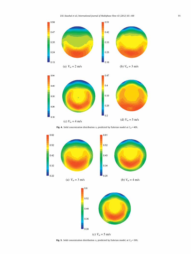
Fig. 4. Solid concentration distribution as predicted by Eulerian model at Cvf = 40%.

(a) Vm = 3 m/s (b) Vm = 4 m/s

(c) Vm = 5 m/s

Fig. 5. Solid concentration distribution as predicted by Eulerian model, at Cvf = 50%.

D.R. Kaushal et al. / International Journal of Multiphase Flow 43 (2012) 85–100 91

-0.5

-0.3

-0.1

0.1

0.3

0.5

y'

C(y')/Cvf

(a) Vm = 1 m/s

-0.5

-0.3

-0.1

0.1

0.3

0.5

y'

C(y')/Cvf

(b) Vm = 2 m/s

-0.5

-0.3

-0.1

0.1

0.3

0.5

y'

C(y')/Cvf

(c) Vm = 3 m/s

-0.5

-0.3

-0.1

0.1

0.3

0.5

0 0.5 1 1.5 2 2.5 0 0.5 1 1.5 2

0 0.5 1 1.5 2 0 0.5 1 1.5 2

y'

C(y')/Cvf

(d) Vm = 4 m/s

y' y'

y' y'

vf

-0.5

-0.3

-0.1

0.1

0.3

0.5

0 0.5 1 1.5 2

y'

C(y')/Cvf

(e) Vm = 5 m/s

Fig. 6. Measured and predicted solid concentration as (0,y) profiles at Cvf = 30%. (N Measured, — Eulerian, ������ Mixture, - - - - - Kaushal and Tomita (2002) AD model)

92 D.R. Kaushal et al. / International Journal of Multiphase Flow 43 (2012) 85–100

equation close to the linear equation, subsequently, using a betterinitial guess.

Parametric analysis was undertaken to assess the sensitivity ofsimulation results to various input parameters and to determineappropriate default parameters and methodologies for predictingthe different properties of slurry flow through pipeline.

4. Experimental equipment

A pilot plant test loop was built in order to obtain data regard-ing various characteristics of the flow of slurry, such as flow rates,pressure drop, flow patterns, and concentration profile across thepipe cross-section. The rig consists of 22 m long, 54.9 mm diameterrecirculating pipe loop, slurry tank, water tank and a centrifugalpump to maintain the slurry flow. The slurry is supplied from theslurry tank, where water and the solid particles are mixed mechan-ically by a mixer powered by an electric motor. The pilot plant testloop is described in detail elsewhere (Kaushal et al., 2005; Kaushaland Tomita, 2007). Spherical glass beads with mean diameters of125 lm and geometric standard deviation of 1.15 have been used

to prepare the slurry. The average specific gravity was measuredas 2.47.

In order to study the settling characteristics of the slurry, mix-ture of various concentrations are prepared. The mixture is kept ina 1000 ml graduated jar. The slurry is thoroughly mixed and thenallowed to settle and also initial level of slurry is recorded. Asthe solid material settles in an undisturbed state, levels of settledslurry in the jar at given intervals of time are noted. Readings aretaken at small interval of time at the beginning and the time inter-val is increased when settling rate slows down. After some time thelevel of settled slurry becomes nearly constant. Various researchersindicate that the optimum concentration of solids for transporta-tion should be about 10–20% points lower than the ultimate staticsettled concentration. In the present study the static settled con-centration was experimentally determined as 63% for glass beadshaving mean diameter of 125 lm. Hence, it was decided to per-form experiments up to a concentration of 50%.

A high performance digital c-ray densitometer (AM870)manufactured by Thermo Electron Corporation Australia mountedon traversing mechanism is used for measurement of

-0.5

-0.3

-0.1

0.1

0.3

0.5

y'

C(y')/Cvf

(a) Vm = 2 m/s

-0.5

-0.3

-0.1

0.1

0.3

0.5

y'

C(y')/Cvf

(b) Vm = 3 m/s

-0.5

-0.3

-0.1

0.1

0.3

0.5

y'

C(y')/Cvf

(c) Vm = 4 m/s

-0.5

-0.3

-0.1

0.1

0.3

0.5

0 0.5 1 1.5 2 0 0.5 1 1.5 2

0 0.5 1 1.5 2 0 0.5 1 1.5 2y'

C(y')/Cvf

(d) Vm = 5 m/s

Fig. 7. Measured and predicted solid concentration as (0,y) profiles at Cvf = 40%. (N Measured, — Eulerian, ������ Mixture, - - - - - Kaushal and Tomita (2002) AD model)

-0.5

-0.3

-0.1

0.1

0.3

0.5

0 0.5 1 1.5 2

y'

C(y')/Cvf

(a) Vm = 3 m/s

-0.5

-0.3

-0.1

0.1

0.3

0.5

0 0.5 1 1.5 2

y'

C(y')/Cvf

(b) Vm = 4 m/s

-0.5

-0.3

-0.1

0.1

0.3

0.5

0 0.5 1 1.5 2

y'

C(y')/Cvf

(c) Vm = 5 m/s

Fig. 8. Measured and predicted solid concentration as (0,y) profiles at Cvf = 50%. (N Measured, — Eulerian, ������ Mixture, - - - - - Kaushal and Tomita (2002) AD model)

D.R. Kaushal et al. / International Journal of Multiphase Flow 43 (2012) 85–100 93

concentration profile. The source and detector are clamped to tra-versing mechanism on either sides of pipeline. A beam of gammaradiation exits from a 3 mm high slit in the source holder contain-ing small radioisotope (Cesium, Cs137), moves through the pipe

with slurry flowing inside and enters the detector unit. Thestrength of the source used was 740 MBq (20mCi). The c-ray den-sitometer is capable of measuring concentration with an accuracyof 0.01%.

(a) Vm = 1 m/s

(b) Vm = 2 m/s

(c) Vm = 3 m/s

(d) Vm = 4 m/s

(e) Vm = 5 m/s

Fig. 9. Velocity distribution tsz(x, y) in m/s predicted by Eulerian model at Cvf = 30%.

94 D.R. Kaushal et al. / International Journal of Multiphase Flow 43 (2012) 85–100

5. Modeling results

5.1. Pressure drop

Pressure drop predictions by both Eulerian and Mixture two-phase models for flow of water as given by Fig. 2 (a), show goodagreement with the experimental data. Comparison betweenmeasured and predicted pressure drops are presented inFig. 2b–d at different concentrations, namely, 30%, 40% and 50%,respectively. From these figures, it is observed that Mixture mod-el fails to predict pressure drops correctly. The amount of errorincreases rapidly with the concentration. However, Eulerianmodel gives fairly accurate predictions for pressure drop at allthe efflux concentrations and flow velocities considered in thepresent study.

5.2. Concentration distribution

Eulerian model results for concentration distribution have beenplotted in Figs. 3–5 at different Cvf and Vm. From these figures, it isobserved that particles are dispersing in such a way that their inter-action with pipe wall is increasing with increase in flow velocity.Further, it is observed that variation of solids concentration in thehorizontal plane becomes more noticeable as the Cvf and flow veloc-ity increases. For most of the data, the higher concentration zone, issituated in the lower half portion at the bottom of pipe, which is dueto the gravitational effect. However, at higher Cvf and flow veloci-ties, the higher concentration zones are situated in the lower halfportion of pipeline away from the surrounding pipe wall.

Figs. 6–8 present the measured and predicted solids concentra-tion profiles using CFD based Mixture and Eulerian models, and

(a) Vm = 1 m/s

(b) Vm = 3 m/s

(c) Vm = 4 m/s

(d) Vm = 5 m/s

Fig. 10. Velocity distribution tsz(x, y) in m/s predicted by Eulerian model at Cvf = 40%.

D.R. Kaushal et al. / International Journal of Multiphase Flow 43 (2012) 85–100 95

Kaushal and Tomita (2002) AD model, where C(y0) is the solids con-centration at different locations y0(=y/D, where, y is the height frompipe centre) in the central vertical plane defined by followingequation:

Cðy=DÞ ¼ 12x

Z x

�xasðx; y=DÞdx ð50Þ

where x takes into account the horizontal or lateral variation of con-centration in pipe cross-section.

The modeling results obtained by Eulerian and Kaushal andTomita (2002) model were found to be in better agreement thanthe Mixture model. It is further observed that both the Mixtureand Kaushal and Tomita (2002) model are unable to predict solidsconcentration profiles with maximum concentration away frompipe bottom due to absence of lift force in both these models.The over prediction of pressure drops shown in Fig. 2 may beattributed to the larger concentrations at pipe bottom shown inFigs. 6–8 by Mixture model due to exclusion of lift force in the Mix-ture model.

5.3. Velocity distribution

Figs. 9–11 show the velocity distributions tsz(x, y) at Cvf of 30%,40% and 50%, respectively, tsz(x, y) is the z-component of solidvelocity perpendicular to the pipe cross-section (x–y plane). It isobserved that at lower Cvf and Vm, the solids velocity distributionis asymmetric having relatively smaller velocities in the lower halfof the pipe due to larger shear force. However, the velocity distri-butions tend to become symmetric as the velocity and concentra-tion increase. The reason for obtaining symmetric velocitydistributions may be attributed to the increased turbulence result-

ing into the complete mixing of fluid and solid particles at higherCvf and Vm.

Fig. 12 shows the distribution of slip-velocity across the verticalplane of the pipe. It is observed that the solid particles move withlower velocities than fluid near the bottom. The slip-velocity keepson increasing with the height from pipe bottom, and reduces at thetop of pipe. It is also observed that the slip-velocities at the bottomof pipe increases with Cvf and Vm. Further, the effect of flow velocityover slip-velocity is prominent at lower concentrations. As the con-centration increases the slip-velocity profiles start coming closer toeach other. The reason for higher concentration zones situating inthe lower half portion of the pipe away from the surrounding pipeboundary at higher Cvf and Vm as shown in Figs. 6–8 may be attrib-uted to the slowing down of solid particles at pipe bottom with re-spect to the surrounding fluid. These decelerated particles have atendency to migrate into the higher Vm zone in the upper layersaway from the bottom of pipe. However, as the slip velocity in-creases with the height from the pipe bottom, this tendency ofmoving upward stops due to the combined effect of gravitationalforces acting vertically downward and reduced velocity differencebetween fluid and solid particles.

5.4. Shear stress distribution

Fig. 13 shows the distribution of z-component of solids shearstress ssz(x, y) at concentrations of 30%, 40% and 50% at differentvelocities, where ssz is ssrz in a cylindrical coordinates (r, h, z) andcalculated as: sxz cos h + syz sin h. It is observed that shear stressdue to solids, which has maximum value near the pipe bottom, in-creases with velocity and concentration. For both the concentra-tions of 30% and 40%, its maximum value is almost doubled for

(a) Vm = 3 m/s (b) Vm = 4 m/s

(c) Vm = 5 m/s

Fig. 11. Velocity distribution tsz(x, y) in m/s predicted by Eulerian model at Cvf = 50%.

(a) Cvf =30%

5 m/s 4 m/s3 m/s 2 m/s1 m/s

-0.5-0.3-0.10.10.30.5

y'

{νsz(0,y) - νfz(0,y)}, m/s

5 m/s 4 m/s3 m/s 2 m/s1 m/s

-0.015 -0.01 -0.005 0 0.005 0.01

96 D.R. Kaushal et al. / International Journal of Multiphase Flow 43 (2012) 85–100

increase in velocity from 3 m/s to 5 m/s. However, at concentrationof 50%, the increase in its maximum value is around 1.2 times. De-crease in shear stress value at the highest concentration may beattributed to the migration of particles from near-wall zone tothe central core of pipe as discussed in the previous article 5.3. Fur-ther, it is observed that at lower velocities, the shear stress has itsprominence at the pipe-bottom and has negligible value at the topof pipe. However, as the velocity increases, shear stress startsshowing its effect all around the pipe-periphery.

5 m/s 4 m/s

3 m/s 2 m/s

-0.5-0.3-0.10.10.30.5

y'

{νsz(0,y) - νfz(0,y)} m/s

(b) Cvf =40%

5 m/s 4 m/s

3 m/s 2 m/s

-0.5-0.3-0.10.10.30.5

-0.015 -0.01 -0.005 0 0.005 0.01

-0.015 -0.01 -0.005 0 0.005 0.01

y'

{νsz(0,y) - νfz(0,y)}, m/s

(c) Cvf =50%

5 m/s4 m/s3 m/s

Fig. 12. Slip-velocity {msz(0,y) � mfz(0,y)} distribution predicted by Eulerian model.

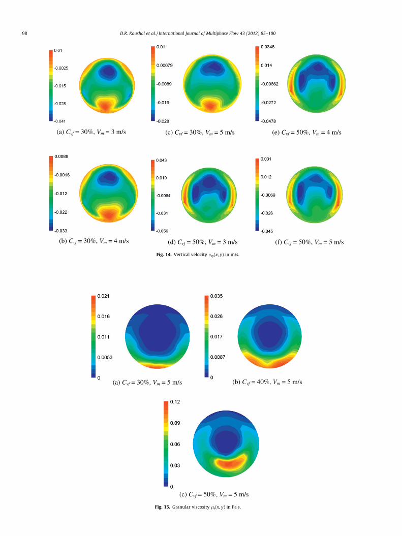
5.5. Vertical velocity distribution

Fig. 14 shows vertical velocity tsy(x, y) distribution at concen-trations of 30% and 50% at different velocities. It is observed thatin the lower half of pipe, particles have tendency to move upward.In the upper half of pipe, particles tend to fall downward due togravitational effect. The upward particle velocities near the pipe-wall result into the shifting of maximum concentration pointsaway from pipe bottom as observed experimentally also at higherconcentrations and velocities. However, since in the advection–diffusion equation, sediment diffusivity and settling velocity actsalways in vertically upward and downward direction, respectively,the AD equation cannot predict a distribution with negative con-centration gradient, although it may reproduce a distribution witha negligible concentration gradient at pipe bottom due to increasedconcentration. It is evident in Figs. 6–8. In this sense, a correctedAD equation is desirable.

Euler model seems to tell that the driving force of particles is thedrag force due to the negative slip velocity. If the average kineticenergy equations of both phases are derived from the momentum

(a) Cvf = 30%, Vm = 3 m/s

(d) Cvf = 30%, Vm = 4 m/s

(g) Cvf = 30%, Vm = 5 m/s

(b) Cvf = 40%, Vm = 3 m/s

(e) Cvf = 40%, Vm = 4 m/s

(h) Cvf = 40%, Vm = 5 m/s

(c) Cvf = 50%, Vm = 3 m/s

(f) Cvf = 50%, Vm = 4 m/s

(i) Cvf = 50%, Vm = 5 m/s

Fig. 13. Shear stress ssz(x, y) in Pa.

D.R. Kaushal et al. / International Journal of Multiphase Flow 43 (2012) 85–100 97

equations, the transfer of energy from water to particles will beshown. There must be energy source in some region and sink ofenergy of particles motion. Guess is that; in the lower part of pipecross-section particle concentration is high and the slip velocity isnegative, which means the energy is transferred from water to par-ticles, and that energy will be transferred to the upper part, whichaccelerates the particles higher than the water in the upper part.

5.6. Granular viscosity and pressure distributions

Figs. 15 and 16 show granular viscosity ls(x, y) distribution at5 m/s and granular pressure Ps(x, y) distribution at 3, 4 and 5 m/s,respectively, with concentrations of 30%, 40% and 50% at eachvelocity. It can be seen from Fig. 15 that the granular viscosity in-creases rapidly with concentration and velocity. It reaches 120times of molecular viscosity of water for the highest concentrationof 50%, at velocity of 5 m/s. Further, that the maximum granularviscosity occurs away from the pipe bottom only at concentration

of 50% results into the wall shear-stress less sensitive to the veloc-ity in comparison with the lower concentrations of 30% and 40%,where the granular viscosity is maximum at pipe bottom. How-ever, granular pressures are always found to be maximum atpipe-bottom as shown in Fig. 16. As expected, granular pressureeffects are limited only to the near pipe-bottom zone at lowerconcentrations and velocities due to movement of lesser numberof particles with lower turbulence intensities.

5.7. Comparison of granular and non-granular mathematical modeling

It is seen that the granular (or solids) concentration varieswidely across the pipe cross-section as shown in Fig. 17, where/t and /t+dt are the energies associated with a particle at time tand t + dt, respectively. For the granular phase, it is clear that anymathematical model, which pretends modeling a granular flow,must account for the following effects, at any time and anywherewithin the flow:

(a) Cvf = 30%, Vm = 3 m/s

(b) Cvf = 30%, Vm = 4 m/s

(c) Cvf = 30%, Vm = 5 m/s

(d) Cvf = 50%, Vm = 3 m/s

(e) Cvf = 50%, Vm = 4 m/s

(f) Cvf = 50%, Vm = 5 m/s

Fig. 14. Vertical velocity tsy(x, y) in m/s.

(a) Cvf = 30%, Vm = 5 m/s (b) Cvf = 40%, Vm = 5 m/s

(c) Cvf = 50%, Vm = 5 m/s

Fig. 15. Granular viscosity ls(x, y) in Pa s.

98 D.R. Kaushal et al. / International Journal of Multiphase Flow 43 (2012) 85–100

(a) Cvf = 30%, Vm = 3 m/s

(d) Cvf = 30%, Vm = 4 m/s

(g) Cvf = 30%, Vm = 5 m/s

(b) Cvf = 40%, Vm = 3 m/s.

(e) Cvf = 40%, Vm = 4 m/s

(h) Cvf = 40%, Vm = 5 m/s

(c) Cvf = 50%, Vm = 3 m/s

(f) Cvf = 50%, Vm = 4 m/s

(i) Cvf = 50%, Vm = 5 m/s

Fig. 16. Granular pressure Ps(x, y) due to particle interaction in Pa.

Fig. 17. Pictorial explanation of kinetic, collisional and frictional viscosities.

D.R. Kaushal et al. / International Journal of Multiphase Flow 43 (2012) 85–100 99

� In the dilute part of the flow, grains randomly fluctuate andtranslate, this form of viscous dissipation and stress is namedkinetic.

� At higher concentration, in addition to the above dissipationform, grains can collide shortly, this gives rise to furtherdissipation and stress, named collisional.

� At very high concentration (50% in volume), grains start toendure long, sliding and rubbing contacts, which gives riseto a totally different from of dissipation and stress, namedfrictional.

However, these viscous dissipations are considered nonexistentin case of non-granular modeling. In Tables 1a and 1b, experimen-tal and computed pressure drops for granular and non-granularmodeling are tabulated. It is seen that the percentage error forgranular modeling ranges up to 15%, whereas for non-granularmodeling, it reaches up to 70%.

Table 1aComparison of experimental and computed pressure drops for granular mathematical modelling.

Cvf (%) Vm (m/s) Experimental Computed pressure drops with different combinations of stresses (kPa)

dP/L (kPa/m) GR + DF GR + DF + LF GR + DF + VM GR + DF + VM + LF % Error

30 3 1.99 2.34 2.27 2.34 2.00 0.314 3.43 4.11 3.96 4.11 3.50 1.845 5.35 5.88 5.64 5.88 4.99 6.55

40 3 2.23 2.88 2.81 2.88 2.48 11.284 3.79 5.07 4.85 5.01 4.35 14.695 6.39 7.25 6.89 7.13 6.21 2.88

50 3 3.41 3.43 3.35 3.43 2.97 13.054 4.78 6.02 5.75 5.90 5.20 8.815 7.22 8.62 8.14 8.38 7.42 2.87

Table 1bComparison of experimental and computed pressure drops for non-granular mathematical modelling.

Cvf (%) Vm (m/s) Experimental Computed pressure drops with different combinations of stresses (kPa)

dP/L (kPa/m) NONG + DF NONG + DF + LF NONG + DF + VM NONG + DF + VM + LF % Error

30 3 1.99 1.06 1.03 1.06 0.91 54.604 3.43 1.91 1.84 1.91 1.63 52.635 5.35 2.76 2.65 2.76 2.35 56.08

40 3 2.23 1.12 1.09 1.12 0.97 56.674 3.79 2.03 1.94 2.01 1.74 54.045 6.39 2.94 2.79 2.89 2.52 60.65

50 3 3.41 1.19 1.16 1.19 1.03 69.904 4.78 2.15 2.05 2.11 1.85 61.185 7.22 3.11 2.94 3.02 2.68 62.87

NONG: Non-granular.GR: Granular.DF: Drag force.LF: Lift force.VM: Virtual mass.

100 D.R. Kaushal et al. / International Journal of Multiphase Flow 43 (2012) 85–100

6. Conclusions

Following conclusions have been drawn on the basis of presentstudy:

1. Mixture model fails to predict pressure drops correctly. Theamount of error increases rapidly with the slurryconcentration.

2. Eulerian model gives fairly accurate predictions for pressuredrop at all the efflux concentrations and flow velocities.

3. The concentration distributions obtained using Eulerianmodel found to be in good agreement except for few exper-imental data near the pipe bottom.

4. The lateral variation of solids concentration in the pipecross-section is more dominant at higher concentrationsand flow velocities.

5. The higher concentration zone at higher velocities and con-centrations is situated in the lower half portion of pipelineaway from the surrounding pipe boundary.

6. At lower velocities and concentrations, the higher concen-tration zone is situated in the lower half portion at the bot-tom of slurry pipeline.

7. Most of the particles migrate due to slip velocity in the cen-tral core of pipeline at higher concentrations and flow veloc-ities, resulting into the central concentrations higher thanthe concentration near pipe wall.

References

Campbell, C.S., Francisco, A.S., Liu, Z., 2004. Preliminary observations of a particle liftforce in horizontal slurry flow. Int. J. Multiph. Flow 30, 199–216.

FLUENT, 2005. User’s guide FLUENT 6.2, Fluent Incorporation, USA.Gidaspow, D., Bezburuah, R., Ding, J., 1992. Hydrodynamics of circulating fluidized

beds, kinetic theory approach in fluidization VII. In: Proceedings of the 7thEngineering Foundation Conference on Fluidization.

Kaushal, D.R., Tomita, Y., 2007. Experimental investigation of near-wall lift ofcoarser particles in slurry pipeline using c-ray densitometer. Powder Technol.172, 177–187.

Kaushal, D.R., Sato, K., Toyota, T., Funatsu, K., Tomita, Y., 2005. Effect of particle sizedistribution on pressure drop and concentration profile in pipeline flow ofhighly concentrated slurry. Int. J. Multiphase Flow 31, 809–823.

Kaushal, D.R., Tomita, Y., 2002. Solids concentration profiles and pressure drop inpipeline flow of multisized particulate slurries. Int. J. Multiphase Flow 28,1697–1717.

Launder, B.E., Spalding, D.B., 1974. The numerical computation of turbulent flows.Comput. Methods Appl. Mech. Eng. 3, 269–289.

Ling, J., Skudarnov, P.V., Lin, C.X., Ebadian, M.A., 2003. Numerical investigations ofliquid–solid slurry flows in a fully developed turbulent flow region. Int. J. HeatFluid Flow 24, 389–398.

Lun, C.K.K., Savage, S.B., Jeffrey, D.J., Chepurniy, N., 1984. Kinetic theories forgranular flow: inelastic particles in couette flow and slightly inelastic particlesin a general flow field. J. Fluid Mech. 140, 223–256.

Thinglas, T., Kaushal, D.R., 2008a. Comparison of two dimensional and threedimensional CFD modeling of invert trap configuration to be used in sewer solidmanagement. Particuol, Else. Publ. 6, 176–184.

Thinglas, T., Kaushal, D.R., 2008b. Three dimensional CFD modeling for optimizationof invert trap configuration to be used in sewer solid management. ParticulateScience and Technology, 26. Taylor and Francis Publications, pp. 507–519.