56
| Date post: | 05-Apr-2018 |
| Category: |
Documents |
| Upload: | duongkhuong |
| View: | 215 times |
| Download: | 2 times |


International Journal of Innovations in Materials Science and Engineering (IMSE)
VOLUME 1, NUMBER 2 July 2014
Preface
This Special Issue of the International Journal of Innovation in Materials Science and Engineering is a collection of a few selected manuscripts in the areas of Mechanical, Civil and Materials Engineering presenting analyses and computational methods, as well as experimental studies of engineering problems of structural vibrations whose solutions focus on strategies for optimizing or quantifying the damping of the system at the propagating disturbance. This short collection of works is meant to give to the reader an overview of different vibrations problems that can be found in diverse areas of Engineering. Particularly, the common aspect linking these works is the way these problems have been or can be solved or analyzed by proposing innovative solutions, in terms of novel materials or systems, and methods for the analysis, detection and optimization of the damping of vibrations in these very diverse applications. Five of these manuscripts are the extended versions of articles accepted and included in the Mini‐Symposium MS26 ‐ Development of Materials and Systems for Vibrations Damping ‐ of the 11th biennial International Conference on vibration Problems (ICOVP‐2013) held in Lisbon in September 9‐12, 2013. The event was jointly organized by the Department of Civil Engineering of the Faculdade de Ciências e Tecnologia of the Universidade Nova of Lisbon FCT/UNL, and IDMEC, the Institute of Engineering Mechanics of the Instituto Superior Técnico of the Technical University of Lisbon (IST/UTL) and the Institute of Engineering Mechanics of the Instituto Superior Técnico of the Technical University of Lisbon (IST/UTL). I would like to thank all the authors for their contributions to this Special Issue, Fabrizia Ghezzo Shenzhen, P.R. China, July 2014.
Tel: +1 (613) 663‐9646, Fax: +1 (613) 801‐1406
PO Box 72032, 4048 Carling Ave, Ottawa, ON, K2K 2P4, Canada
JOURNAL OF INNOVATION IN MATERIALS SCIENCE AND ENGINEERING (IMSE) 1
Electrorheological Fluid Power Dissipation and Requirements for anAdaptive Tunable Vibration Absorber
Nicklas Norrick1
1Institute of Structural Dynamics, Technische Universitat Darmstadt, Darmstadt, Germany
Electrorheological fluid (ERF) is an adaptive material which changes its material properties quickly and reversibly in response toan electric field. The effect was discovered by Winslow in 1947. The change in apparent material behavior makes ERF interestingfor use in the on-line tuning of dynamic systems such as tuned vibration absorbers (TVAs). In this paper, an adaptive multibodyabsorber prototype filled with ERF is investigated. Its performance is evaluated experimentally and a numerical model is validatedwith the measurements. Special focus on power requirements and efficiency of the semi-active tuning mechanism. The multibodyadaptive TVA prototype consists of a closed plastic casing, in which two rigid bodies are suspended via elastic helical springs.Two independent high-voltage channels allow the application of up to 6000 V in narrow gaps between the absorber bodies andthe absorber casing, influencing the material properties of the ERF. Experiments show the continuous change of the apparent firstnatural frequency and corresponding damping of the absorber in response to the applied high voltages. A mathematical model ofthe prototype including a nonlinear description of the ER material behavior is presented. An extended BINGHAM model is used todescribe the behavior of the ERF under influence of an electric field. Using the validated numerical model, the absorber performanceon a virtual test system and the power dissipation in the absorber can be calculated. The power dissipation is compared to themeasured power requirements of the ERF and the power consumption of the high voltage amplifiers. The efficiency of the ERmaterial to induce damping is very shown to be very high. In contrast, the efficiency of the high voltage amplifiers used in theexperiments is very low. The results can help foster further developments of adaptive TVAs and other semi-active devices utilizingERF as an adjustment mechanism.
Index Terms—Electrorheological Fluid, ERF, Tuned Vibration Absorber, Semi-Active
I. INTRODUCTION
Passive vibration absorbing devices have been used instructural dynamics for over a century, first patented by Frahmfor the damping of ship roll [1]. Since Den Hartog [2]developed the theory of the optimal tuned vibration absorber(TVA), the governing equations have been the subject matterof fundamental structural dynamics courses around the world.It is well-known that the classical TVA is only capable ofquenching vibrations at its tuning frequency. When excitationfrequencies of a system or system properties change duringoperation, the mistuned absorber may exhibit worse behaviorthan the original system without the absorber. To overcomethis flaw, much research has been presented regarding activeor semi-active TVAs.
Using electrorheological fluids (ERF), the natural frequencyand damping characteristics of a multibody tuned vibrationabsorber can be changed to achieve vibration attenuation overa broad frequency band.
Preumont gives a concise definition of semi-active devices:
”Semi-active control devices are essentially passive deviceswhere properties (stiffness, damping, ...) can be adjusted inreal time, but they cannot input energy directly in the systembeing controlled” [3].
Because of this, semi-active devices have certain advantagesover fully active systems. First, semi-active devices requirevery little energy in comparison with an active system forthe same reduction in vibration amplitudes. Second, since
Corresponding author: N. Norrick (email: [email protected]).
semi-active devices cannot serve as a source of energy forthe system they are influencing, destabilization due to faultycontrol parameters or a failure in the system is generallynot a problem. Hrovat offers a comprehensive comparisonof the characteristics of passive, semi-active and active TVAperformance [4].
Since Winslow discovered the electrorheological effectnearly seventy years ago [5], [6], many researchers haveused electrorheological materials to influence dynamic sys-tems. Bullough and Foxon [7] used adaptive electrorheologicaldampers for the control of unwanted vibrations.
The magnetorheological effect creates very similar changesin the material behavior of magnetorheological fluids (MRF),which have also been studied extensively for the use inadjustable dampers. Recent work by Sims et al. [8] is anexample from academia. The LORD Corporation has beenmarketing industrial products utilizing this technology for overa decade [9].
For TVAs the change in material behavior exhibited byeither ERF or MRF has been investigated experimentally andtheoretically. Janocha and Jendritza [10] first presented a pro-totype TVA with adjustable damping characteristics utilizingelectrorheological fluid. Sloshing-type vibration absorbers forcivil engineering applications have been studied by Truongand Semercigil [11] and Sakamoto et al. [12]. Both groupshave presented experimental results using ERF as a sloshingliquid in a tank. Truong and Semercigil noted a change solelyin the damping characteristic of the TVA while Sakamotoet al. presented a design that makes it possible to changethe effective mass of the absorber and thereby influence theabsorber’s natural frequency. Koo [13] used MRF dampers in a
International Journal of Innovations in Materials Science and Engineering (IMSE), VOL. 1, NO. 2 49
© 2014 EDUGAIT Press
JOURNAL OF INNOVATION IN MATERIALS SCIENCE AND ENGINEERING (IMSE) 2
prototype of a semi-active TVA and presented both theoreticaland experimental results highlighting the advantages of thesemi-active system over classical passive TVAs. Instead ofMRF, Holdhusen [14] used magnetorheological elastomers(MRE) to design a semi-active TVA with adaptive stiffness,in turn facilitating a change in absorber natural frequency.Several research groups have discussed the change in a sand-wich beam’s stiffness with ERF or MRF and done extensivetheoretical and experimental work. Earliest work was doneby Choi et al. [15]. Only recently has the change in beamstiffness been used to change absorber natural frequency on-line by Hirunyapruk [16]. Sun and Thomas used a modified ro-tational viscometer as an electrorheological dynamic torsionalabsorber to effectively reduce torsional rotor vibrations of theviscometer rotor [17].
The subject of this paper is an existing prototype semi-active TVA, designed to fit into the steering wheel of aluxury automobile and influence lateral vibrations in thesteering wheel plane. In previous work, it has been proventhat the natural frequency and damping of this prototypecan be changed by applying electrical field strengths of upto 6 kV/mm [18], [19]. The prototype has also been fittedto an automobile substructure to test the system in nearlyreal conditions. Comprehensive measurements validated theprototype’s performance when the automobile substructurewas subjected to harmonic and white noise excitation [20].To quantify the advantage of a semi-active TVA compared tofully active solutions, this paper concentrates on the powerconsumption and efficiency (defined as the ratio of powerdissipation of the ”smart” material to its power consumption)of the mentioned prototype.
II. MULTIBODY TVA PROTOTYPE
The prototype TVA investigated in this study consists of aclosed plastic casing, in which two bodies are suspended viasets of helical springs. The coupling body (mass m1), has only10% of the mass of the main body (mass m2). Modal analysisof the empty prototype was used to validate the analyticallypredicted natural frequencies of the system.
In the narrow gaps (∼1 mm) between the coupling bodyand the casing a high voltage U1 can be applied, while in thenarrow gaps between the coupling body and the main bodya different high voltage U2 can be applied. Both voltages aresupplied by independently controlled high voltage amplifiers,each up to 6000 V.
The ER material used in this study is a suspension ofpolyurethane particles with an average diameter of 3µm insilicone oil. The solid particle content is Φ=42%.
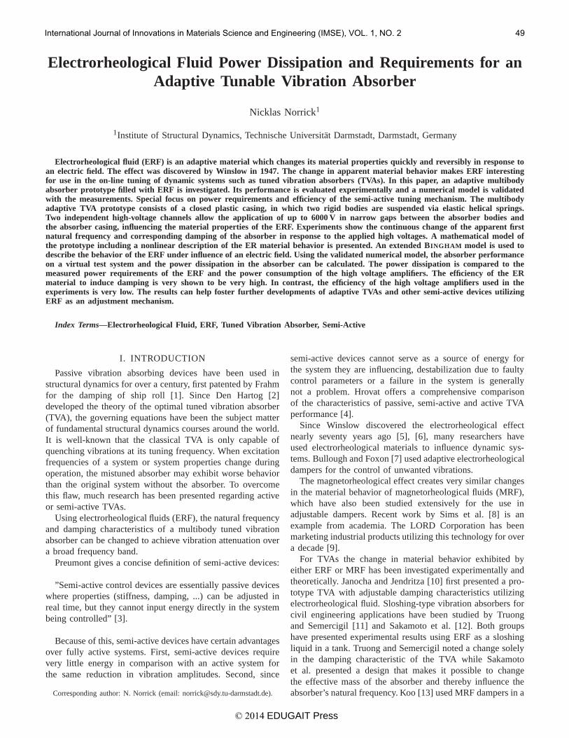
The casing of the absorber is filled with ERF under a slightoverpressure to prevent the formation of air bubbles, whichhave a negative effect on the dielectric strength of the material.A photograph of the prototype is shown in Fig. 1.
The prototype was tested on a vibration testing table. Adetailed diagram of the test rig is shown in Fig. 2. A real-timecontrol system (dSpace DS1103) is used for data acquisitionand the output of the control signals for the two high-voltagegenerators and the frequency signal Ω for the drive motor. The
High voltage cable Displacement sensorand cable
40 mm
Fig. 1. Photograph of the multibody tunable vibration absorber prototype
drive motor induces a nearly harmonic displacement excitationwith a fixed amplitude via a crankshaft. The table displacementu(t) and relative displacement qr(t) of the main absorberbody inside the plastic housing are measured with eddy-currentdisplacement sensors. In addition to the table displacement,a piezoelectric accelerometer on the table records the tableacceleration u(t). The actually applied high voltages U1 andU2 (each up to 6000 V) are controlled and logged throughoutthe experiments. All of the acquired signals are filtered viaidentical analog low-pass filters to eliminate aliasing errors.
Because of the high voltages used in the experiments,special attention must be placed on the connection of theprototype and all components used during measurement to theelectrical ground. Most importantly, we want to minimize therisk of electrical shock for people working in the lab. Addi-tionally, sensitive measurement electronics must be protectedfrom electrostatic discharges which can produce erroneousmeasurements (a minor side effect) or destroy expensivelaboratory equipment.
The test setup allows the measurement of the complexfrequency response
H(Ω) =qr(Ω)
u(Ω)(1)
of the TVA prototype with amplitude |H(Ω)| and phase ψ(Ω).A fixed excitation amplitude u= 0.4mm was chosen for allmeasurements.
III. MATHEMATICAL MODEL
An idealized mechanical model of the absorber is shown inFig. 3. The casing (shown in white) houses the coupling mass(dark gray) and the main mass (light gray). The application ofthe high voltage U1 or U2 influences the ERF and can achieve ablockage of the spring-damper set 1 or 2, respectively, therebyinfluencing system damping and natural frequencies.
To model the influence of the ERF, a nonlinear extendedBINGHAM-type model based on viscometer measurements isused. The model parameters are the electric field strength Eel
and the shear rate γ. The shear stress τERF is the sum of the
International Journal of Innovations in Materials Science and Engineering (IMSE), VOL. 1, NO. 2 50

JOURNAL OF INNOVATION IN MATERIALS SCIENCE AND ENGINEERING (IMSE) 3
u
qr
u
Ω
testing table
drivemotor
adaptive TVA prototype
dSpace PC
A/D
low-pass filtersamplifiers
U1
U2
Fig. 2. Schematic diagram of the vibration test rig with TVA and measuring equipment
u q1
q2=qr
m1
m2
k1 k2
b1 b2
U1 U2
Fig. 3. Sketch of the multibody tunable vibration absorber model
field-dependent yield stress τy and a viscous part,
τERF (Eel, γ) = τy(Eel) + µ(Eel) γ . (2)
The yield stress τy must be exceeded for motion to occur.The values of τy(Eel) and µ(Eel) are determined by fittingthe model to the aforementioned viscometer measurements(crosses in Fig. 4a) using the least-square method for electricalfield values from 0 to 6 kV/mm.
The shear rate is assumed to be directly proportional to theshear stress, consistent with the assumption of a NEWTONianfluid. Since the energy density in an electrical field
eel =1
2ε ε0E
2
el , (3)
is proportional to the square of the electrical field strength aquadratic ansatz for the influence of the electrical field strengthon the shear stress is plausible [21]. The equations
τy(Eel) = aτE2
el (4)
andµ(Eel) = µ0 + aµE
2
el (5)
are used to describe the relationship between the electrical fieldstrength and the yield stress τy and the post-yield viscosityµ, respectively. The result of the fitting of the model to theviscometer measurements is shown in Fig. 4 on the left.
Extensive measurements at the Institute of Structural Dy-namics at the Technische Universitat Darmstadt [22] haveshown that the transition from blockage to flow of the ERF isnot sudden, as the basic BINGHAM model would suggest, butrather a smooth progression. To account for this, the arctan-function is used to smooth the jump in the shear stress atthe shear rate γ = 0. This form function has the additionaladvantage that numerical simulations do not have to cope withthe discontinuity presented by the BINGHAM model. In Fig. 4on the right is a zoom of the area where the influence ofthe arctan-function is clearly visible. The shear stress is nowgiven by
τERF (Eel, γ) =[τy(Eel) + µ(Eel) γ
] 2π
arctan
(c
γ
γmax
),
(6)so that the electrode area A can then be used to calculate aresulting ERF force with the simple product
FERF = τERF A . (7)
International Journal of Innovations in Materials Science and Engineering (IMSE), VOL. 1, NO. 2 51

JOURNAL OF INNOVATION IN MATERIALS SCIENCE AND ENGINEERING (IMSE) 4
γ in 1/s γ in 1/s
τ ERF
inN
/m2
6 kV5 kV4 kV3 kV2 kV1 kV0 kV
2000
1000
-2000
-1000
τ ERF
inN
/m2
1000
-1000
600-600 -50 50
(b)(a)
Fig. 4. Shear stress due to shear rate with BINGHAM-type model (a) and zoom of the interesting area showing the effect of multiplication with the arctan-function (b)
In our case, the effective electrode area A = 8657mm2.The enclosed area in a force-displacement diagram is thedamping work done by one vibration cycle. Multiplication ofthe damping work with the frequency f (in Hz) yields thedamping power P (in W)
P =
∮ −→FERF
−→ds f . (8)
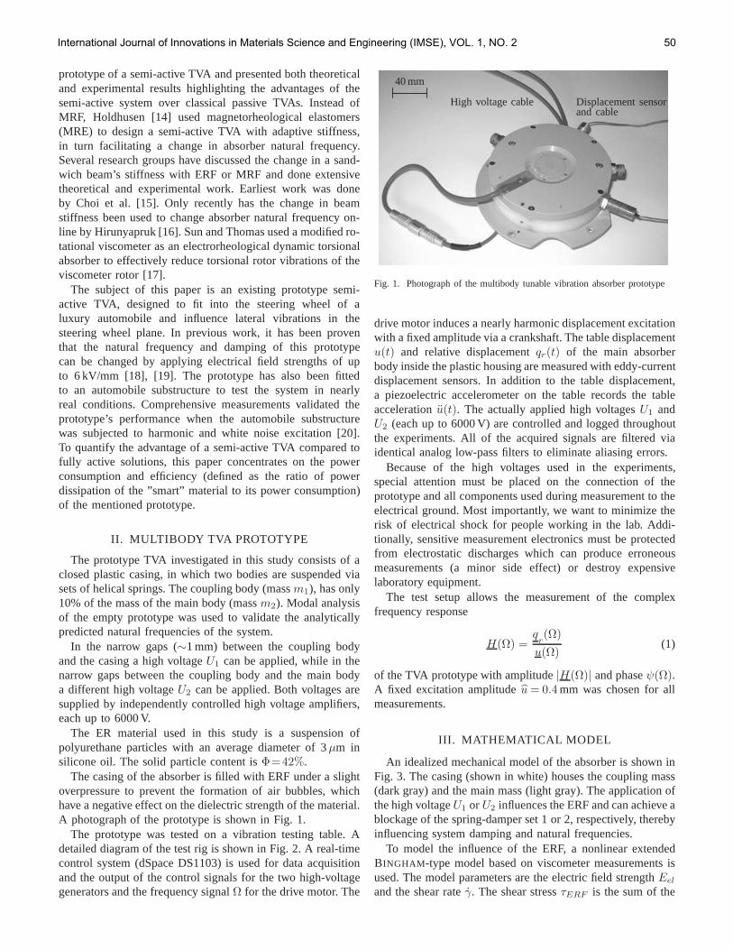
The shown model for the semi-active tuned vibration absorberand the electrorheological material has been parameterized andvalidated by vibration response measurements with differenttypes of excitation [23]. The model reproduces the measureddynamic behavior of the absorber under influence of appliedhigh voltage extremely well. Two examples of the qualityof the model are shown in Figures 5 and 6. Visible is themeasured and simulated system frequency response (amplitude|H(Ω)| and phase ψ(Ω)) of the absorber prototype due to baseexcitation with a constant amplitude and 4000 V applied toeither channel 1 or channel 2 respectively. For comparison,the best linear model is shown as well (dotted line). Thediscrepancy between the linear model and the measurementsis most evident in the amplitude response between about 10and 20 Hz.
A variation of the applied voltage alters the resonancefrequency of the absorber in a range between 18.4 and 24.9 Hz.This can clearly be seen in the measured frequency responsecurves for increasing voltages in Figures 7 and 8. These showthe frequency response of the absorber main body for risinghigh voltages applied to channel 1 and channel 2, respectively.In both figures, a drop in the resonance frequency is visiblebetween the two curves for 0 V and 2000 V. This drop isdue to a change in the added mass of the ERF. From that
0
π
0
1
2
0
|H(Ω
)|ψ(Ω
)
Ω/2π in Hz 50
U1=4 kVU2=0 kV
experimentlinear modelBINGHAM model
Fig. 5. Measured and simulated displacement amplitude |H(Ω)| and phaseψ(Ω) for the absorber prototype due to base excitation, U1= 4 kV and U2=0 kV
point on, an increase in high voltage results in an increasedresonance frequency. The response curves for both cases aresimilar because of the large ratio m2/m1 and the comparablemagnitude of the spring stiffnesses k1 and k2.
A closer look at the simple model from Fig. 3 can helpexplain this: When high voltage is applied to channel 1, theERF in the gap between main body and coupling body blocks
International Journal of Innovations in Materials Science and Engineering (IMSE), VOL. 1, NO. 2 52
JOURNAL OF INNOVATION IN MATERIALS SCIENCE AND ENGINEERING (IMSE) 5
0
π
0
1
2
0
|H(Ω
)|ψ(Ω
)
Ω/2π in Hz 50
U1=0 kVU2=4 kV
experimentlinear modelBINGHAM model
Fig. 6. Measured and simulated displacement amplitude |H(Ω)| and phaseψ(Ω) for the absorber prototype due to base excitation, U1= 0 kV and U2=4 kV
the compliance of spring k1, thereby increasing the apparentnatural frequency of the absorber. Ideally, when m1 −→ 0 andk1=k2 we will have a base natural frequency of
ωbase =
√k22m2
. (9)
A complete blocking of spring k1 will result in a naturalfrequency of
ω1 =
√k2m2
=√2ωbase , (10)
yielding an increase in natural frequency with the factor√2.
When high voltage is applied to channel 2, an analogous effectblocks the compliance of spring k2, resulting in the samefrequency ratio
ω2 =
√k1m2
=√2ωbase . (11)
The measurements show that the prototype absorber attains afrequency ratio of 1.35, quite close to the ideal ratio of
√2.
IV. APPLICATION OF THE ABSORBER TO AHARMONICALLY EXCITED SYSTEM
The validated model can also be used to apply the virtualabsorber to a vibrating system and evaluate the semi-activesystem’s vibration reduction potential. Let us look at a simplecase and apply the tunable absorber to a one-degree-of-freedom system with a natural frequency of 20 Hz and 2%damping. For this example, the system mass is msys=10 kg,about 10 times the absorber mass, a common ratio for TVAs.The resulting parameters are the stiffness ksys = 158 kN/mand damping bsys = 50Ns/m. The system is subjected toharmonic force excitation F (t) = F cos(Ωt). Due to theER material behavior under influence of the electrical field,
U1
0
π
0
1
2
0
|H(Ω
)|ψ(Ω
)
Ω/2π in Hz 50
6 kV4 kV2 kV0 kV
Fig. 7. Measured displacement amplitude |H(Ω)| and phase ψ(Ω) for theabsorber prototype due to base excitation, U1=0 to 6 kV and U2=0kV
U2
0
π
0
1
2
0
|H(Ω
)|ψ(Ω
)
Ω/2π in Hz 50
6 kV4 kV2 kV0 kV•
••
•
Fig. 8. Measured displacement amplitude |H(Ω)| and phase ψ(Ω) for theabsorber prototype due to base excitation, U1=0kV and U2=0 to 6 kV
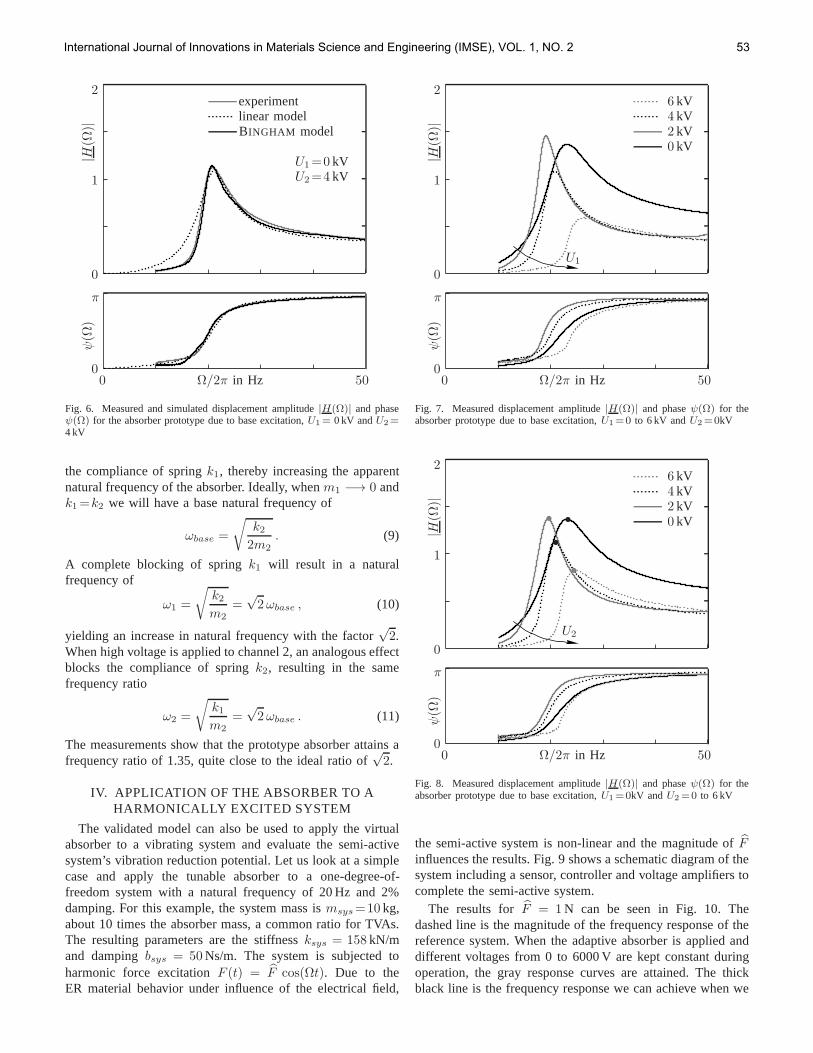
the semi-active system is non-linear and the magnitude of Finfluences the results. Fig. 9 shows a schematic diagram of thesystem including a sensor, controller and voltage amplifiers tocomplete the semi-active system.
The results for F = 1N can be seen in Fig. 10. Thedashed line is the magnitude of the frequency response of thereference system. When the adaptive absorber is applied anddifferent voltages from 0 to 6000 V are kept constant duringoperation, the gray response curves are attained. The thickblack line is the frequency response we can achieve when we
International Journal of Innovations in Materials Science and Engineering (IMSE), VOL. 1, NO. 2 53

JOURNAL OF INNOVATION IN MATERIALS SCIENCE AND ENGINEERING (IMSE) 6
msys
bsys ksys
F (t)
TVA prototype
Controller
Sensor
U1
U2
Fig. 9. Schematic diagram of the one-degree-of-freedom system with appliedTVA prototype
suppose that the high voltage applied to the TVA is optimallyswitched depending on excitation frequency, for example bya simple feed forward control algorithm.
For very large force excitation amplitudes, on the order ofF =100N, the yield stress of the ER material is too small toshow a visible effect on the absorber natural frequency andthe net effect of the semi-active absorber on the system is thatof an adjustable viscous damper.
To quantify the response due to broadband excitation, wecan calculate the area under the response amplitude curvesin a frequency band from 10 to 30 Hz for the system with-out absorber, with a passive absorber (corresponding to novoltage applied) and the optimally switching semi-active ab-sorber. The resulting values are 0.05 mm/Ns for the systemwithout absorber, 0.0474 mm/Ns for the passive system and0.0198 mm/Ns for the semi-active system. The passive ab-sorber achieves a broadband reduction of only 5%, whereasthe semi-active system attains a reduction of 60%.
These numbers quantify the great advantage of the semi-active system. If the power needed to induce this switch insystem behavior is small, the resulting efficiency of the deviceis high. In the following sections, we will therefore focus onpower dissipation and power consumption of the ER material.
V. POWER DISSIPATION IN THE ERF
The power dissipation in the ERF cannot be measureddirectly, but can be calculated from the hysteretic force-displacement diagrams created with the validated model.Because of the previously discussed inherent symmetry ofthe prototype’s dynamic behavior, we will only alter thehigh voltage of channel 2 (U2) in the following studies. Twodistinct cases will be discussed, and because of symmetry,the findings apply to channel 1 as well.
Case 1:
The vibration absorber is tuned to a varying excitationfrequency via high voltage U2. The base excitation amplitudeu is assumed to be constant. The points of operation for eachhigh voltage are marked with bullets (•) in Fig. 8.
Case 2:
The vibration absorber is subjected to a fixed excitationfrequency of Ω/2π=30Hz. The base excitation amplitude uis constant. The applied high voltage U2 is increased from 0to 6000 V.
Fig. 11 shows the calculated force-displacement and force-velocity characteristic obtained from the extended BINGHAM-type model for Case 1. In this case, the system parameters andexcitation frequency change from one voltage to the next, sothe displacement qr of the absorber body is diminished withrising voltages.
Fig. 12 shows the calculated force-displacement and force-velocity characteristic obtained from the extended BINGHAM-type model for Case 2. For this parameter set, the systemresponse amplitude qr remains nearly constant with the excep-tion of a change in system behavior from linear (no voltageapplied) to non-linear (high voltage applied). In both cases,the damping work per cycle increases visibly in accordancewith the increase in high voltage.
From this data, the damping power for these different pointsof operation is calculated and shown in Fig. 13. The quadratictrend of the data for Case 2 is due to Eq. (4) and the fact thatthe displacement amplitude qr is constant. This trend is notevident in the data for Case 1 because of the aforementionedchange in the displacement amplitude qr.
During the course of the experiments, it was postulated thatthe dissipated energy in the prototype absorber would heatthe ERF and thereby change the material’s damping proper-ties during operation. To test this, a temperature probe wasmounted inside the housing during operation near resonanceand the ERF temperature was monitored over a period of22 minutes from a starting point of 25.4 C. Fig. 15 showsthe results where it is evident that the induced change intemperature is negligible.
VI. POWER CONSUMPTION OF THE SEMI-ACTIVESYSTEM
The power needed to create the electrical fields is verylow. Because the ERF is an isolator with a conductivity of10−7 S/m, the currents flowing through the material are of theorder 1 mA. This can be verified by measuring the electricalcurrent during operation with different high voltages. Theutilized laboratory-grade high voltage amplifiers support bothvoltage and current monitoring. The power consumption forsteady-state, direct current operation can be calculated simplyas the product of voltage and current,
P = UI =U2
R. (12)
International Journal of Innovations in Materials Science and Engineering (IMSE), VOL. 1, NO. 2 54
JOURNAL OF INNOVATION IN MATERIALS SCIENCE AND ENGINEERING (IMSE) 7
Excitation frequency Ω/(2π) in Hz
0
0.1
0 10 20 30 40 50
system without TVA
system with optimally switching TVA
system with TVA for different voltages
|Hsys(Ω
)|in
mm
/N
Fig. 10. Calculated system response of a one-degree-of-freedom system due to harmonic force excitation with the absorber prototype applied
qr in mm qr in m/s
FERF
inN
FERF
inN
..... 0 kV2 kV4 kV6 kV
Fig. 11. Case 1: Calculated force-displacement and force-velocity diagrams for the ERF, high voltages U2 from 0 to 6000 V applied, harmonic excitation atresonance frequency
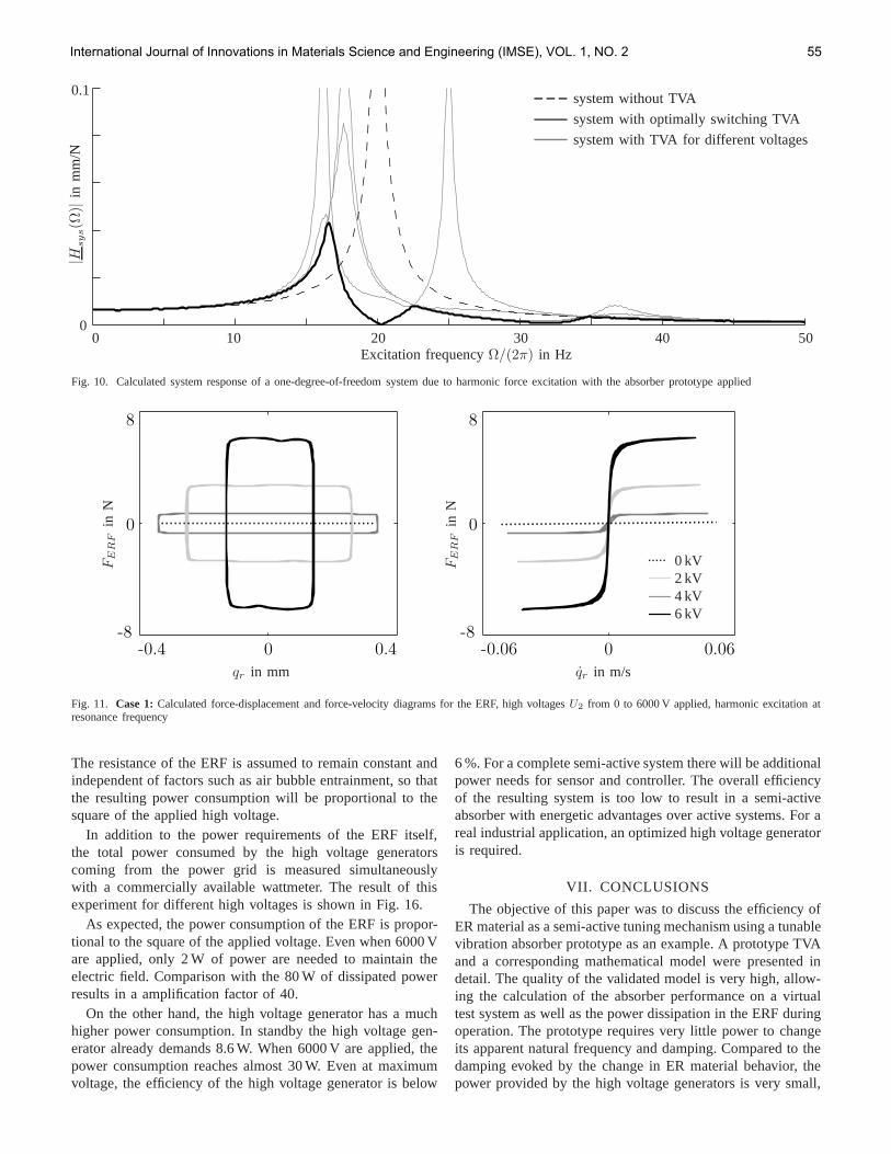
The resistance of the ERF is assumed to remain constant andindependent of factors such as air bubble entrainment, so thatthe resulting power consumption will be proportional to thesquare of the applied high voltage.
In addition to the power requirements of the ERF itself,the total power consumed by the high voltage generatorscoming from the power grid is measured simultaneouslywith a commercially available wattmeter. The result of thisexperiment for different high voltages is shown in Fig. 16.
As expected, the power consumption of the ERF is propor-tional to the square of the applied voltage. Even when 6000 Vare applied, only 2 W of power are needed to maintain theelectric field. Comparison with the 80 W of dissipated powerresults in a amplification factor of 40.
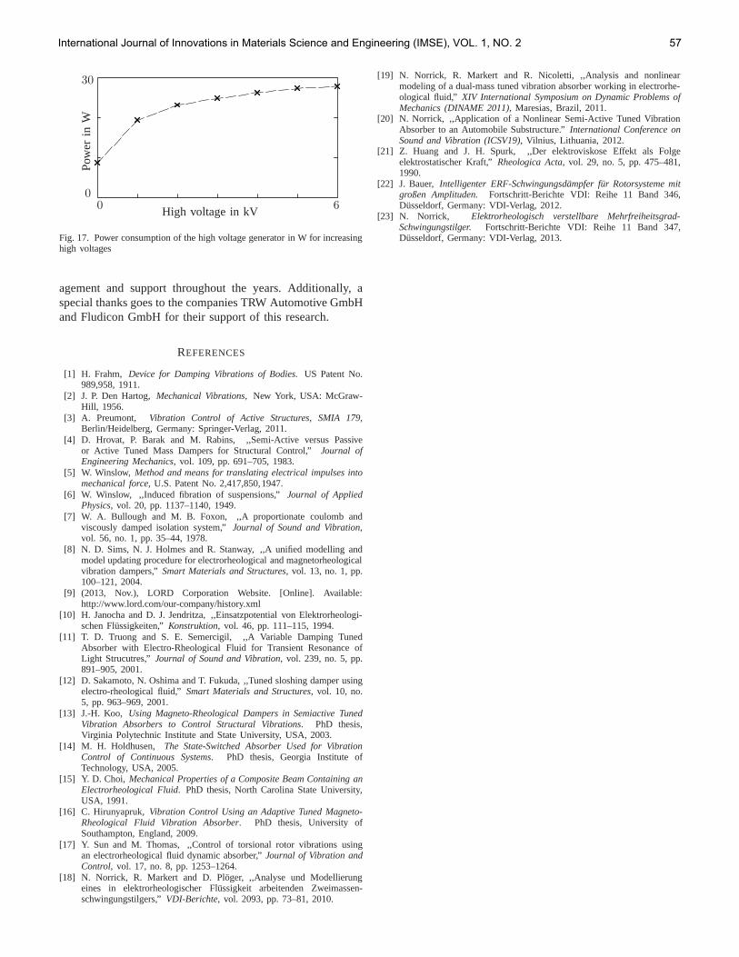
On the other hand, the high voltage generator has a muchhigher power consumption. In standby the high voltage gen-erator already demands 8.6 W. When 6000 V are applied, thepower consumption reaches almost 30 W. Even at maximumvoltage, the efficiency of the high voltage generator is below
6 %. For a complete semi-active system there will be additionalpower needs for sensor and controller. The overall efficiencyof the resulting system is too low to result in a semi-activeabsorber with energetic advantages over active systems. For areal industrial application, an optimized high voltage generatoris required.
VII. CONCLUSIONS
The objective of this paper was to discuss the efficiency ofER material as a semi-active tuning mechanism using a tunablevibration absorber prototype as an example. A prototype TVAand a corresponding mathematical model were presented indetail. The quality of the validated model is very high, allow-ing the calculation of the absorber performance on a virtualtest system as well as the power dissipation in the ERF duringoperation. The prototype requires very little power to changeits apparent natural frequency and damping. Compared to thedamping evoked by the change in ER material behavior, thepower provided by the high voltage generators is very small,
International Journal of Innovations in Materials Science and Engineering (IMSE), VOL. 1, NO. 2 55

JOURNAL OF INNOVATION IN MATERIALS SCIENCE AND ENGINEERING (IMSE) 8
qr in mm qr in m/s
FERF
inN
FERF
inN
..... 0 kV2 kV4 kV6 kV
Fig. 12. Case 2: Calculated force-displacement and force-velocity diagrams for the ERF, high voltages U2 from 0 to 6000 V applied, harmonic excitation atfixed frequency Ω/2π=30Hz
0
90
0 6High voltage in kV
Pow
erin
W
Fig. 13. Calculated power dissipation in the ERF in W for different appliedhigh voltages U2, Case 1
0
90
0 6High voltage in kV
Pow
erin
W
Fig. 14. Calculated power dissipation in the ERF in W for different appliedhigh voltages U2, Case 2
resulting in a high efficiency of the semi-active mechanism.Measurements of power consumption and numerical resultsfor the corresponding power dissipation were presented. Itwas shown that the efficiency of the high voltage generatorsused in this study is too low for the semi-active absorberto exhibit its full potential. The power requirements of thehigh voltage generator can in part be attributed to the specialvoltage and current monitors supplied by the laboratory unitused for these measurements. Future development of semi-
0
40
0 22Operation time in minutes
ER
Fte
mpe
ratu
rein
C
Fig. 15. Measured ERF temperature during operation with applied highvoltage in resonance conditions in C
0
2
0 6High voltage in kV
Pow
erin
W
Fig. 16. Power consumption of the ERF in W for increasing high voltages
active devices using ERF as an adjustment mechanism mustincorporate this knowledge into the design process to ensurecompetitiveness.
VIII. ACKNOWLEDGEMENTS
The author would like to thank Prof. Dr.-Ing. RichardMarkert for the fruitful discussions and his constant encour-
International Journal of Innovations in Materials Science and Engineering (IMSE), VOL. 1, NO. 2 56
JOURNAL OF INNOVATION IN MATERIALS SCIENCE AND ENGINEERING (IMSE) 9
0
30
0 6High voltage in kV
Pow
erin
W
Fig. 17. Power consumption of the high voltage generator in W for increasinghigh voltages
agement and support throughout the years. Additionally, aspecial thanks goes to the companies TRW Automotive GmbHand Fludicon GmbH for their support of this research.
REFERENCES
[1] H. Frahm, Device for Damping Vibrations of Bodies. US Patent No.989,958, 1911.
[2] J. P. Den Hartog, Mechanical Vibrations, New York, USA: McGraw-Hill, 1956.
[3] A. Preumont, Vibration Control of Active Structures, SMIA 179,Berlin/Heidelberg, Germany: Springer-Verlag, 2011.
[4] D. Hrovat, P. Barak and M. Rabins, ,,Semi-Active versus Passiveor Active Tuned Mass Dampers for Structural Control,” Journal ofEngineering Mechanics, vol. 109, pp. 691–705, 1983.
[5] W. Winslow, Method and means for translating electrical impulses intomechanical force, U.S. Patent No. 2,417,850,1947.
[6] W. Winslow, ,,Induced fibration of suspensions,” Journal of AppliedPhysics, vol. 20, pp. 1137–1140, 1949.
[7] W. A. Bullough and M. B. Foxon, ,,A proportionate coulomb andviscously damped isolation system,” Journal of Sound and Vibration,vol. 56, no. 1, pp. 35–44, 1978.
[8] N. D. Sims, N. J. Holmes and R. Stanway, ,,A unified modelling andmodel updating procedure for electrorheological and magnetorheologicalvibration dampers,” Smart Materials and Structures, vol. 13, no. 1, pp.100–121, 2004.
[9] (2013, Nov.), LORD Corporation Website. [Online]. Available:http://www.lord.com/our-company/history.xml
[10] H. Janocha and D. J. Jendritza, ,,Einsatzpotential von Elektrorheologi-schen Flussigkeiten,” Konstruktion, vol. 46, pp. 111–115, 1994.
[11] T. D. Truong and S. E. Semercigil, ,,A Variable Damping TunedAbsorber with Electro-Rheological Fluid for Transient Resonance ofLight Strucutres,” Journal of Sound and Vibration, vol. 239, no. 5, pp.891–905, 2001.
[12] D. Sakamoto, N. Oshima and T. Fukuda, ,,Tuned sloshing damper usingelectro-rheological fluid,” Smart Materials and Structures, vol. 10, no.5, pp. 963–969, 2001.
[13] J.-H. Koo, Using Magneto-Rheological Dampers in Semiactive TunedVibration Absorbers to Control Structural Vibrations. PhD thesis,Virginia Polytechnic Institute and State University, USA, 2003.
[14] M. H. Holdhusen, The State-Switched Absorber Used for VibrationControl of Continuous Systems. PhD thesis, Georgia Institute ofTechnology, USA, 2005.
[15] Y. D. Choi, Mechanical Properties of a Composite Beam Containing anElectrorheological Fluid. PhD thesis, North Carolina State University,USA, 1991.
[16] C. Hirunyapruk, Vibration Control Using an Adaptive Tuned Magneto-Rheological Fluid Vibration Absorber. PhD thesis, University ofSouthampton, England, 2009.
[17] Y. Sun and M. Thomas, ,,Control of torsional rotor vibrations usingan electrorheological fluid dynamic absorber,” Journal of Vibration andControl, vol. 17, no. 8, pp. 1253–1264.
[18] N. Norrick, R. Markert and D. Ploger, ,,Analyse und Modellierungeines in elektrorheologischer Flussigkeit arbeitenden Zweimassen-schwingungstilgers,” VDI-Berichte, vol. 2093, pp. 73–81, 2010.
[19] N. Norrick, R. Markert and R. Nicoletti, ,,Analysis and nonlinearmodeling of a dual-mass tuned vibration absorber working in electrorhe-ological fluid,” XIV International Symposium on Dynamic Problems ofMechanics (DINAME 2011), Maresias, Brazil, 2011.
[20] N. Norrick, ,,Application of a Nonlinear Semi-Active Tuned VibrationAbsorber to an Automobile Substructure.” International Conference onSound and Vibration (ICSV19), Vilnius, Lithuania, 2012.
[21] Z. Huang and J. H. Spurk, ,,Der elektroviskose Effekt als Folgeelektrostatischer Kraft,” Rheologica Acta, vol. 29, no. 5, pp. 475–481,1990.
[22] J. Bauer, Intelligenter ERF-Schwingungsdampfer fur Rotorsysteme mitgroßen Amplituden. Fortschritt-Berichte VDI: Reihe 11 Band 346,Dusseldorf, Germany: VDI-Verlag, 2012.
[23] N. Norrick, Elektrorheologisch verstellbare Mehrfreiheitsgrad-Schwingungstilger. Fortschritt-Berichte VDI: Reihe 11 Band 347,Dusseldorf, Germany: VDI-Verlag, 2013.
International Journal of Innovations in Materials Science and Engineering (IMSE), VOL. 1, NO. 2 57

The Optimization and Sensitivity Analysis of Sandwich Plates
E. Kormaníková*1, K. Kotrasová
1
1
Abstract This paper presents the optimization and sensitivity
analysis of a sandwich plate whose laminate facings failure is
predicted by applying the criterion of Tsai-Wu. A symmetric
sandwich plate is optimized with the objective functions of
maximizing the natural frequencies and maximizing the buckling
load. The design variables are the fiber orientation of the
individual outer layers and are computed by using the Sequential
Linear Programming method and the Modified Feasible
Direction method. The sensitivity analysis is similar, in principle,
to the design optimization. In the sensitivity analysis the design
variables are changed between their lower and upper bounds in a
specified number of steps.
Keywords Buckling Analysis, Free Vibration Analysis,
Optimization, Sensitivity Analysis, Sandwich Plate, Tsai-Wu
Criterion
I. INTRODUCTION
aterial that is a mixture of two or more distinct
constituents or phases is a composite material, in which
must be fulfillment that all constituents have to be presented in
reasonable proportions and have quite different properties
from the properties of the composite material. One very
important group of laminated composites are sandwich
composites. Sandwich composites consist of two thin facings
sandwiching a core. The facings are made of a material that
has high strength (metals or fiber reinforced laminates), which
can transfer axial forces and bending moments, while the core
is generally made of lightweight materials such as foam, resins
with special fillers, alder wood etc. The material used in a
sandwich core must be resistant to compression and capable of
transmitting shear [1].
In the present paper we optimize a symmetric sandwich
plate with laminated angle-ply facings. The design variables
are the fiber orientations of the laminated facings. The
objectives of the design are the maximization of the natural
frequencies and the maximization of the buckling load. The
Tsai-Wu constraint must be satisfied in order to have a
feasible design. Optimization problem is formulated as a
nonlinear programming problem.
The sandwich plate is taken to be rectangular and simply
supported. The static analysis is performed in two steps. First,
a finite element method is used to determine the overall
buckling load of the sandwich plate. Using FEM formulation
[2, 12], the first ten buckling loads are solved numerically.
The second part of the analysis is free vibration analysis.
Within this analysis the first ten natural frequencies are
solved.
The optimization and sensitivity of a composite plate are
very important analyses for design of structures ranging from
aircrafts to civil structures.
II. STATIC ANALYSIS OF SANDWICH PLATES
To formulate the governing differential equations for
sandwich plates we utilize the similarity of the elastic
behaviour between laminates and sandwiches within the first
order shear deformation theory applied to sandwich plates. We
restrict our considerations to symmetric sandwich plates with
thin cover sheets. There are differences in the expressions for
the flexural stiffness, coupling stiffness and the transverse
shear stiffness of laminates and sandwiches [3]. Furthermore
there are essential differences in the stress distributions.
The assumptions on the deformations are:
a) For the sandwich thin cover sheets are valid
Kirchhoff´s assumptions on deformations. In-plane
stress-strain state is accrued in the sandwich thin
cover sheets.
b) The sandwich core with the thickness h2 transfers
only shear stresses perpendicular to the mid-plane of
the cover sheets. The needed material property is the
shear modulus G2.
c) All points in the normal line have the equal
deflections w1 = w2 = w3 = w.
d) All layers are perfectly bonded.
We can write the shear deformations (Fig. 1) [4, 5] as
follows
x
w
h
d
h
uu
x
w
h
uuxz
22
31
2
32122
,
y
w
h
d
h
vv
y
w
h
vvyz
22
31
2
32122
, (1)
where d is the distance -planes.
2
312
hhhd . (2)
y
z
h2
h1
h3 w
yz,2
w/ y
v12
v32
d
w/ y
x
z
h2
h1
h3 w
xz,2
w/ x
u12
u32
d
w/ x
Fig. 1. Geometry of deformation
M
International Journal of Innovations in Materials Science and Engineering (IMSE), VOL. 1, NO. 2 58
© 2014 EDUGAIT Press

There are the normal forces (Fig. 2) in cover sheets i = 1, 3
y
v
x
uDN i
ii
Niix
, y
v
x
uDN ii
iiNiy
,
x
v
y
uDN iiiNi
ixy2
)1( ,
where
)1/( 2
iiiNi hED . (3)
The bending moments and the shear forces in the skins (Fig.
2) we can write as
2
2
2
2
y
w
x
wDM iMiix
, 2
2
2
2
y
w
x
wDM iMiiy
,
yx
wDM iMiixy
2
1 ,
2
3
3
3
yx
w
x
wDV Miixz
, yx
w
y
wDV Miiyz 2
3
3
3
,
where
)1(12/ 23
iiiMi hED . (4)
The shear stresses in the core are written
x
wduu
h
GG xzxz 31
2
222
,
y
wdvv
h
GG yzyz 31
2
222
. (5)
The equilibrium equations for internal forces are the following
0z
V
y
N
x
N zxiyxixi , 0z
V
y
N
x
N zyiyixyi ,
i =1,3
0py
V
x
V yzxz ,
where
zxzx
z
V 1 , zx
zx
z
V 3 ,
z
V
y
M
x
MV xzxyxxz
, z
V
y
M
x
MV
yzyyx
yz,
2hz
Vxz
xz , 2h
z
Vyz
yz . (6)
To solve the unknown functions u1(x,y), u3(x,y), v1(x,y),
v3(x,y), w(x,y) it is necessary to set the boundary conditions for
each boundary [9-11].
We have used the finite element method for solving the
problem. The continuum was divided into a finite number of
rectangular finite plate elements.
h3
h3/2
x,u3
z,w
2
Mx1
Mx1+Mx1,x
h2
h1
d
x,u1
Vxz3+Vxz3,x
Nx3
Mx3
Nx3+ N3i,x
xzh2
Nx1
Vxz1+Vxz1,x
Nx1+ Nx1,x
xz
zx
1 Nxy1
3
Nxy3
z,w
Mx3+Mx3,x
Vxz3
( xz + xz,x )h2
Vxz1
Fig. 2. Internal forces at the sandwich element in the (x, z) plane
III. FREE VIBRATION AND BUCKLING ANALYSIS OF
SANDWICH PLATE
The equations to determine the natural frequencies of a
symmetric sandwich panel are following 2 2 2
11 66 12 662 2
2
55 2
( )
0,s
D D D Dx y x y
wk A I
x t
(7)
2 2 2
12 66 66 222 2
2
44 2
( )
0,s
D D D Dx y x y
wk A I
y t
(8)
2 2
55 442 2
2
20,
s s
m
w wk A k A
x x y y
w
t
(9)
( ) ( 1)
1
3( ) 3 ( 1) 3
1
1( ),
1( ) ( ) ,
12 3
Nk k
m k
k
Nk km
k
k
h
I
(10)
where
ks is the transverse shear deformation factor given by value 5/6
for quasi-isotropic laminate,
k is the mass density of the kth layer.
For the simply supported plate let
´
1 1
( , , ) sin sin ,mni t
mn
m n
mw x y t C e
a b
´
1 1
( , , ) cos sin ,mni t
mn
m n
mx y t A e
a b
´
1 1
( , , ) sin cos ,mni t
mn
m n
mx y t B e
a b (11)
where
m, n are integers only,
a, b are the panel dimensions in x, y axis direction
respectively,
International Journal of Innovations in Materials Science and Engineering (IMSE), VOL. 1, NO. 2 59
mn is natural angular velocity.
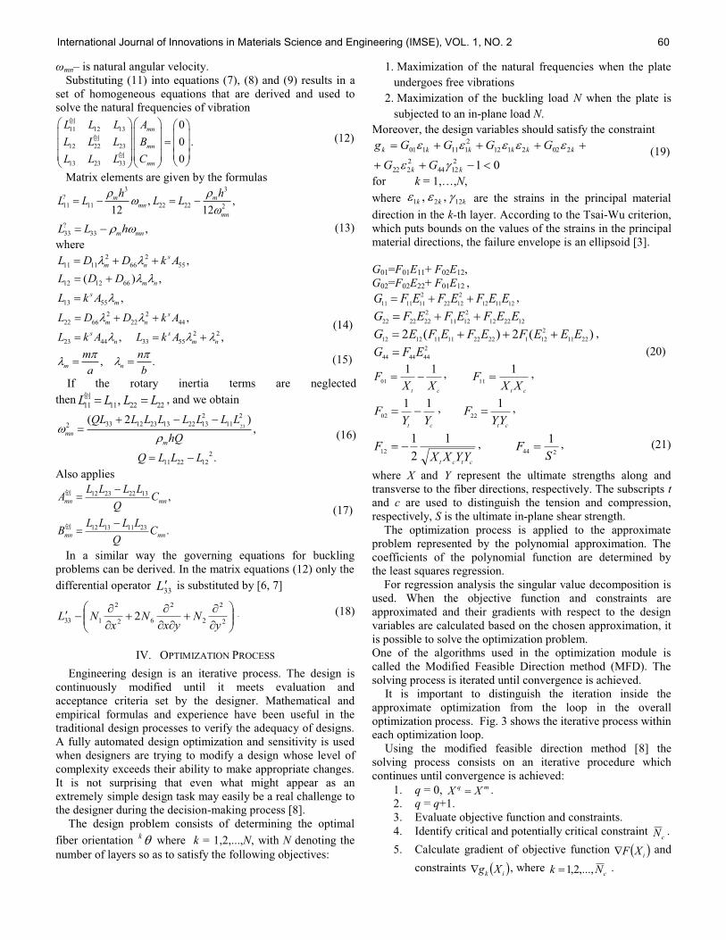
Substituting (11) into equations (7), (8) and (9) results in a
set of homogeneous equations that are derived and used to
solve the natural frequencies of vibration
11 12 13
12 22 23
13 23 33
0
0 .
0
mn
mn
mn
L L L A
L L L B
L L L C
(12)
Matrix elements are given by the formulas 3 3
?
11 11 22 22 2, ,
12 12
m mmn
mn
h hL L L L
?
33 33 ,m mnL L h
(13)
where 2 2
11 11 66 55
12 12 66
13 55
,
( ) ,
,
s
m n
m n
s
m
L D D k A
L D D
L k A
2 2
22 66 22 44
2 2
23 44 33 55
,
, ,
s
m n
s s
n m n
L D D k A
L k A L k A
(14)
, .m n
m n
a b
(15)
If the rotary inertia terms are neglected
then11 11 22 22,L L L L , and we obtain
23
2 2
33 12 23 13 22 13 112
2
11 22 12
( 2 ),
.
mn
m
QL L L L L L L L
hQ
Q L L L
(16)
Also applies
12 23 22 13
12 13 11 23
,
.
mn mn
mn mn
L L L LA C
Q
L L L LB C
Q
(17)
In a similar way the governing equations for buckling
problems can be derived. In the matrix equations (12) only the
differential operator 33L is substituted by [6, 7]
2
2
2
2
62
2
133 2y
Nyx
Nx
NL . (18)
IV. OPTIMIZATION PROCESS
Engineering design is an iterative process. The design is
continuously modified until it meets evaluation and
acceptance criteria set by the designer. Mathematical and
empirical formulas and experience have been useful in the
traditional design processes to verify the adequacy of designs.
A fully automated design optimization and sensitivity is used
when designers are trying to modify a design whose level of
complexity exceeds their ability to make appropriate changes.
It is not surprising that even what might appear as an
extremely simple design task may easily be a real challenge to
the designer during the decision-making process [8].
The design problem consists of determining the optimal
fiber orientation k
where k = 1,2,...,N, with N denoting the
number of layers so as to satisfy the following objectives:
1. Maximization of the natural frequencies when the plate
undergoes free vibrations
2. Maximization of the buckling load N when the plate is
subjected to an in-plane load N.
Moreover, the design variables should satisfy the constraint
012
1244
2
222
2022112
2
111101
kk
kkkkkk
GG
GGGGg (19)
for k N,
where kkk 1221 ,, are the strains in the principal material
direction in the k-th layer. According to the Tsai-Wu criterion,
which puts bounds on the values of the strains in the principal
material directions, the failure envelope is an ellipsoid [3].
G01=F01E11+ F02E12,
G02=F02E22+ F01E12 ,
121112
2
1222
2
111111EEFEFEFG ,
122212
2
1211
2
222222EEFEFEFG
)(2)(22211
2
121222211111212EEEFEFEFEG ,
2
444444EFG (20)
ctXX
F11
01,
ctXX
F1
11,
ctYY
F11
02,
ctYY
F1
22,
ctctYYXX
F1
2
112
, 244
1
SF , (21)
where X and Y represent the ultimate strengths along and
transverse to the fiber directions, respectively. The subscripts t
and c are used to distinguish the tension and compression,
respectively, S is the ultimate in-plane shear strength.
The optimization process is applied to the approximate
problem represented by the polynomial approximation. The
coefficients of the polynomial function are determined by
the least squares regression.
For regression analysis the singular value decomposition is
used. When the objective function and constraints are
approximated and their gradients with respect to the design
variables are calculated based on the chosen approximation, it
is possible to solve the optimization problem.
One of the algorithms used in the optimization module is
called the Modified Feasible Direction method (MFD). The
solving process is iterated until convergence is achieved.
It is important to distinguish the iteration inside the
approximate optimization from the loop in the overall
optimization process. Fig. 3 shows the iterative process within
each optimization loop.
Using the modified feasible direction method [8] the
solving process consists on an iterative procedure which
continues until convergence is achieved:
1. q = 0, mq XX .
2. q = q+1.
3. Evaluate objective function and constraints.
4. Identify critical and potentially critical constraint cN .
5. Calculate gradient of objective function iXF and
constraints ik Xg , where
cNk ,...,2,1 .
International Journal of Innovations in Materials Science and Engineering (IMSE), VOL. 1, NO. 2 60

6. Find a usable-feasible search direction qS .
7. Perform a one-dimensional search qqq SXX 1 .
8. Check convergence. If satisfied, make qm XX 1 .
Otherwise, go to 2.
9. qm XX 1 .
The convergence of MFD to the optimum is checked by
several criteria. There are the criterion of maximum of
iterations and criterion of changes of objective function.
Besides the previously mentioned criteria, the Kuhn-Tucker
conditions necessary for optimality must be satisfied.
SLP and
MFD
Methods
Parametric
geometry and
mesh
) 1 (
i x
Initial analysis
Postprocessing
Define Design variables Objective function Behavior constraints
m=1
Update geometry
and mesh (if
needed) ) ( m i x
Perform analysis
Approximate objective function
and constraints
Improved design ) 1 ( m
i x
m=m+1
yes Requirements no achieved ?
Optimization loop
General optimization
Fig. 3. General optimization process
A. Unconstrained Problems
The conditions degenerate to the case where the gradient of
the objective function vanishes
0XF . (22)
It is noted that this condition is necessary but not sufficient for
optimality. To ensure a function to be a minimum, the Hessian
matrix must by positive-definite.
Also, the optimum is in a sense of relative optimum rather
than global one. In general, the conditions to ensure a global
minimum can rarely be demonstrated. If a global minimum is
intended, one must restart the optimization process from
different initial points to check if other solutions are possible.
Fig. 4 shows the relative and global minima in the design
space.
Fig. 4. Relative and global minima in the design space
B. Constrained Problems
The conditions of optimality are more complex. By using
the Lagrangian multiplier method, we define the Lagrangian
function as the following m
j
jnjjn
k
j
jjn sXXgXXhXXFL1
2
11
1
1 ),...,(),...,(),...,(
(23)
where j, j =1, ...,k and j, j=1, ..., m are Lagrangian
multiplicators and sj is a slack variable which measures how
far the jth constraint is from being critical.
Differentiating the Lagrangian function with respect to all
variables we obtain the Kuhn-Tucker conditions which are
summarized as follows
011
m
j i
j
j
k
j i
j
j
i X
g
X
h
X
F , i = 1, ..., n. (24)
Stationarity with respect to j, j = 1, ... ,k gives the following
restrictions
hj (X1, ..., Xn) = 0, j = 1, ..., k. (25)
Stationarity L with respect to sj, gives jsj = 0 and 22 / jsL
for maximum of F.
The physical interpretation of these conditions is that the
sum of the gradient of the objective function and the scalars j
times the associated gradients of the active constraints must
vectorially add to zero as shown in Fig. 5.
The Kuhn-Tucker conditions are also sufficient for
optimality when the number of active constraints is equal to
the number of design variables. Otherwise, sufficient
conditions require the second derivatives of the objective
function and constraints (Hessian matrix) similar to the
unconstrained one. If the objective function and all of the
constraints are convex, the Kuhn-Tucker conditions are also
sufficient for global optimality [8].
)(XF
)(11 Xg
)(22 Xg
)(2 Xg
)(1 Xg
)(XF
0)(1 Xg
0)(2 Xg
)(XF
X2
X1
Fig. 5. Kuhn-Tucker conditions at a constrained optimum
We conducted a sensitivity analysis during and after the
optimization process. A sensitivity study is the procedure that
determines the changes in a response quantity for a change in
a design variable. We used the global sensitivity, where design
variables are changed between their lower and upper bounds
in a specified number of steps.
The other algorithm for solving the nonlinear approximate
optimization problem is called the Sequential Linear
International Journal of Innovations in Materials Science and Engineering (IMSE), VOL. 1, NO. 2 61

Programming method (SLP). The iterative process of SLP
within each optimization loop is shown below:
1. p=0, Xp=Xm.
2. p=p+1.
3. Linearize the problem at 1pX by creating a first
order Taylor Series expansion of the objective function and
retained constraints
)XX)(X(F)X(F)X(F ppp 111
)XX)(X(g)X(g)X(g ppp 111 .
4. Use this approximation of optimization instead of
the original nonlinear functions:
Maximize: F(X)
Subject to: 0)(Xg and U
ii
L
i XXX .
5. Find an improved design pX (using the Modified
Feasible Direction method).
6. Check feasibility and convergence. If both of them
are satisfying, go to 7. Otherwise, go to step 2.
7. pm XX 1 .
Using the SLP method the solving process is iterated until
convergence is achieved. Convergence or termination checks
are performed at the end of each optimization loop in general
optimization. The optimization process continues until either
convergence or termination occurs.
V. TSAI-WU CRITERION
We can distinguish the failure between fiber failure (FF)
and inter fiber failure (IFF). In the case of plane stress, the IFF
criteria discriminates three different modes. The IFF mode A
is when perpendicular transversal cracks appear in the lamina
under transverse tensile stress with or without in-plane shear
stress. The IFF mode B denotes the occurrence of
perpendicular transversal cracks, but in this case they appear
under in-plane shear stress with small transverse compression
stress. The IFF mode C indicates the onset of oblique cracks
when the material is under significant transversal compression
[2].
The strength of a composite layer in any other direction can
be evaluated on various failure criteria. The basic premise in
predicting the failure of fiber-reinforced layers using the
maximum stress and maximum strain criteria is the same as
the one used for isotropic material. Failure is predicted when
the maximum stress along the fiber or transverse to the fiber
directions exceed the strength of the tension or compression.
A more general form of the Tsai-Wu failure criterion for
orthotropic materials under plane stress assumption is
expressed as
12 2
1244
2
2222022112
2
111101FFFFFF (26)
The failure criterion for orthotropic material under strain
assumption is expressed as
12
1244
2
2222022112
2
111101GGGGGG . (27)
When 212
2
1
tX
F , the Tsai-Wu criterion is reduced to Tsai-
Hill criterion, and when
ctXX
F2
112
the Tsai-Wu criterion
is reduced to Hoffman criterion [3].
These failure criteria are used to calculate a failure index
(F.I.) from the computed stresses and user-supplied material
strengths. A failure index denotes the onset of failure, and a
value less than 1 denotes no failure. The failure index
according to this theory is computed using the following
equation [2] 2
1244
2
2222022112
2
111101 2 FFFFFFIF.
(28)
The failure load factor is inverse value to the failure index.
VI. SOLUTION AND RESULTS
Solve the optimization and sensitivity of sandwich plate
(Fig. 6) made of a 6-layer Boron-Epoxy laminated facings
[ 60/60/ ]s and polystyrene core. The thickness h of
the laminate is 0.001 m. The material properties for laminate
layers are given as:
E1 = 194GPa, E2 = 8.7GPa, G12 = 3.2GPa, 12 = 0.33,
2100 kg/m3
Xt = 1300MPa, Xc = 2000MPa, Yt = 140MPa, Yc = 300MPa,
S = 90MPa.
The material properties for sandwich core are given as:
E = 42MPa, = 0.3, 1uMPa, 150 kg/m
3.
The plate is simply supported at all boundaries and loaded
by a uniaxial uniform load (Fig. 6). Thickness h is for the
facings and 8*h is for the core (Fig. 7).
2
1
1 m
2 m
6 nh = h x
z
nh = h/n
-60
+60
+60
-60
y
x
Fig. 6. Geometry of the sandwich plate and staff of facing layers
h 8*h
h Laminate facings
Fig. 7. Cross-section of sandwich plate
International Journal of Innovations in Materials Science and Engineering (IMSE), VOL. 1, NO. 2 62
-0.00335
-0.00336
-0.00337
-0.00338
-0.00339
-0.0034
-0.00341
-0.00342
-0.00344
-0.00345
-0.00346 0 5 10 15 20 25 30 35 40 45 50 55 60 65 70 75 80 85 90
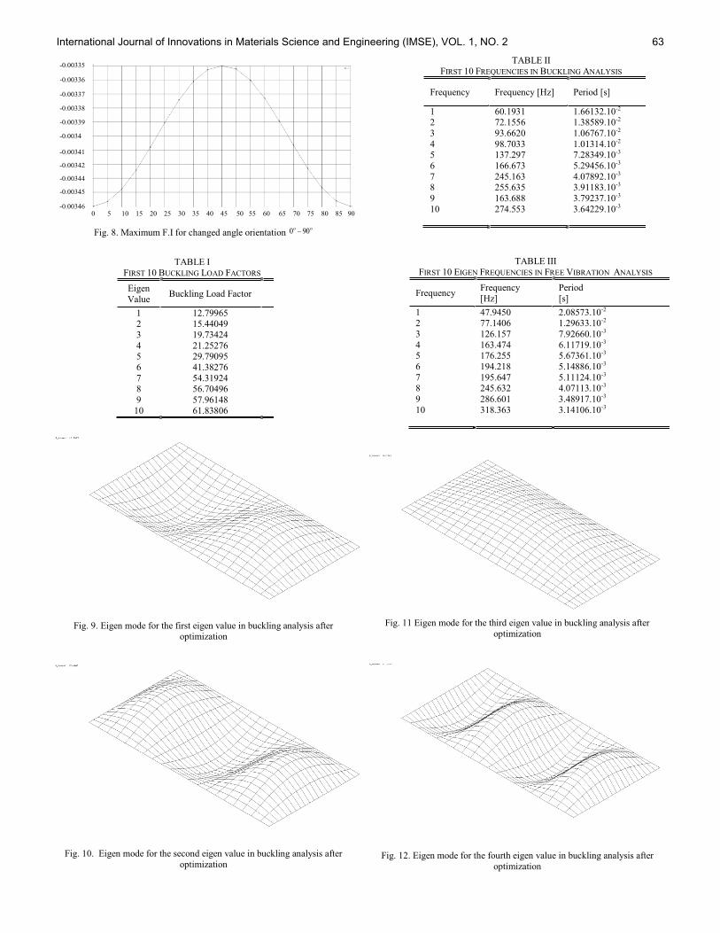
Fig. 8. Maximum F.I for changed angle orientation 900
Fig. 9. Eigen mode for the first eigen value in buckling analysis after optimization
Fig. 10. Eigen mode for the second eigen value in buckling analysis after
optimization
Fig. 11 Eigen mode for the third eigen value in buckling analysis after
optimization
Fig. 12. Eigen mode for the fourth eigen value in buckling analysis after
optimization
TABLE I
FIRST 10 BUCKLING LOAD FACTORS
Eigen
Value Buckling Load Factor
1 12.79965 2 15.44049
3 19.73424
4 21.25276
5 29.79095
6 41.38276
7 54.31924 8 56.70496
9 57.96148
10 61.83806
TABLE III
FIRST 10 EIGEN FREQUENCIES IN FREE VIBRATION ANALYSIS
Frequency Frequency
[Hz]
Period
[s]
1 47.9450 2.08573.10-2
2 77.1406 1.29633.10-2
3 126.157 7.92660.10-3
4 163.474 6.11719.10-3 5 176.255 5.67361.10-3
6 194.218 5.14886.10-3
7 195.647 5.11124.10-3 8 245.632 4.07113.10-3
9 286.601 3.48917.10-3
10 318.363 3.14106.10-3
TABLE II
FIRST 10 FREQUENCIES IN BUCKLING ANALYSIS
Frequency Frequency [Hz] Period [s]
1 60.1931 1.66132.10-2
2 72.1556 1.38589.10-2
3 93.6620 1.06767.10-2
4 98.7033 1.01314.10-2 5 137.297 7.28349.10-3
6 166.673 5.29456.10-3
7 245.163 4.07892.10-3 8 255.635 3.91183.10-3
9 163.688 3.79237.10-3
10 274.553 3.64229.10-3
International Journal of Innovations in Materials Science and Engineering (IMSE), VOL. 1, NO. 2 63

Fig. 13. First eigen mode in free vibration analysis after optimization
Fig. 14. Second eigen mode in free vibration analysis after optimization
Fig. 15. Third eigen mode in free vibration analysis after optimization
Fig. 16. Fourth eigen mode in free vibration analysis after optimization
Fig. 17. Stresses x for the bottom of the lower cover sheet along the mid-
section
Fig. 18. Stresses y
for the bottom of the lower cover sheet along the mid-
section
Fig. 19. Stresses xy
for the bottom of the lower cover sheet along the mid-
section
Fig. 20. Colour plot of displacements u
International Journal of Innovations in Materials Science and Engineering (IMSE), VOL. 1, NO. 2 64
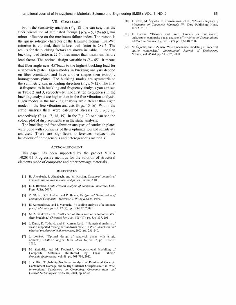
VII. CONCLUSION
From the sensitivity analysis (Fig. 8) one can see, that the
fiber orientation of laminated facings [ 60/60/ ]s has
minor influence on the maximum failure index. The reason is
the quasi-isotropic character of the laminate facings. Tsai-Wu
criterion is violated, than failure load factor is 289.5. The
results for the buckling factors are shown in Table 1. The first
buckling load factor is 22.6 times minor than maximum failure
load factor. The optimal design variable is 45 . It means
that fiber angle near 45 leads to the highest buckling load for
a sandwich plate. Eigen modes in buckling analysis depend
on fiber orientation and have another shapes then isotropic
homogeneous plates. The buckling modes are symmetric to
the symmetric axis in loading direction (Figs. 9-12). The first
10 frequencies in buckling and frequency analysis you can see
in Table 2 and 3, respectively. The first ten frequencies in the
buckling analysis are higher than in the free vibration analysis.
Eigen modes in the buckling analysis are different than eigen
modes in the free vibration analysis (Figs. 13-16). Within the
static analysis there were calculated stresses x , y
, xy
respectively (Figs. 17, 18, 19). In the Fig. 20 one can see the
colour plot of displacements u in the static analysis.
The buckling and free vibration analyses of sandwich plates
were done with continuity of their optimization and sensitivity
analyses. There are significant differences between the
behaviour of homogeneous and heterogeneous materials.
ACKNOWLEDGMENT
This paper has been supported by the project VEGA
1/0201/11 Progressive methods for the solution of structural
elements made of composite and other new-age materials.
REFERENCES
[1] H. Altenbach, J. Altenbach, and W. Kissing, Structural analysis of laminate and sandwich beams and plates, Lublin, 2001.
[2] E. J. Barbero, Finite element analysis of composite materials, CRC
Press, USA, 2007.
[3] Z. Gürdal, R.T. Haftka, and P. Hajela, Design and Optimization of
Laminated Composite Materials, J. Wiley & Sons, 1999.
[4] E. Kormaníková, and I. Mamuzic, Buckling analysis of a laminate plate Metalurgija, vol. 47 (2), pp. 129-132, 2008.
[5] M. Mihaliková et al., Influence of strain rate on automotive steel
sheet breaking Chemické listy, vol. 105 (17), pp. 836-837, 2011.
[6] J. Tóthová, and E. Kormaníková, Numerical analysis of
elastic supported rectangular sandwich plate Proc. Structural and
physical problems of civil structures, 2003, pp. 235-240.
[7] J. , Optimal design of sandwich plates with a rigid
obstacle ZAMM-Z. angew. Math. Mech. 69, vol. 7, pp. 191-201,
1989.
[8] Computational Modelling of
Composite Materials Reinforced by Glass Fibers
Procedia Engineering, vol. 48, pp. 701-710, 2012.
[9] J. Králik, Probability Nonlinear Analysis of Reinforced Concrete
Containment Damage due to High Internal Overpressure, in Proc.
International Conference on Computing, Communications and Control Technologies: CCCT'04, 2004, pp. 65-68.
[10] Selected Chapters of
Mechanics of Composite Materials III., Derc Publishing House U.S.A, 2013.
[11] E. Carrera, Theories and finite elements for multilayered,
anisotropic, composite plates and shells Archives of Computational Methods in Engineering, vol. 9 (2), pp. 87-140, 2002.
[12] and J. Zeman, Micromechanical modeling of imperfect
textile composites International Journal of Engineering Science, vol. 46 (6), pp. 513-526, 2008.
International Journal of Innovations in Materials Science and Engineering (IMSE), VOL. 1, NO. 2 65
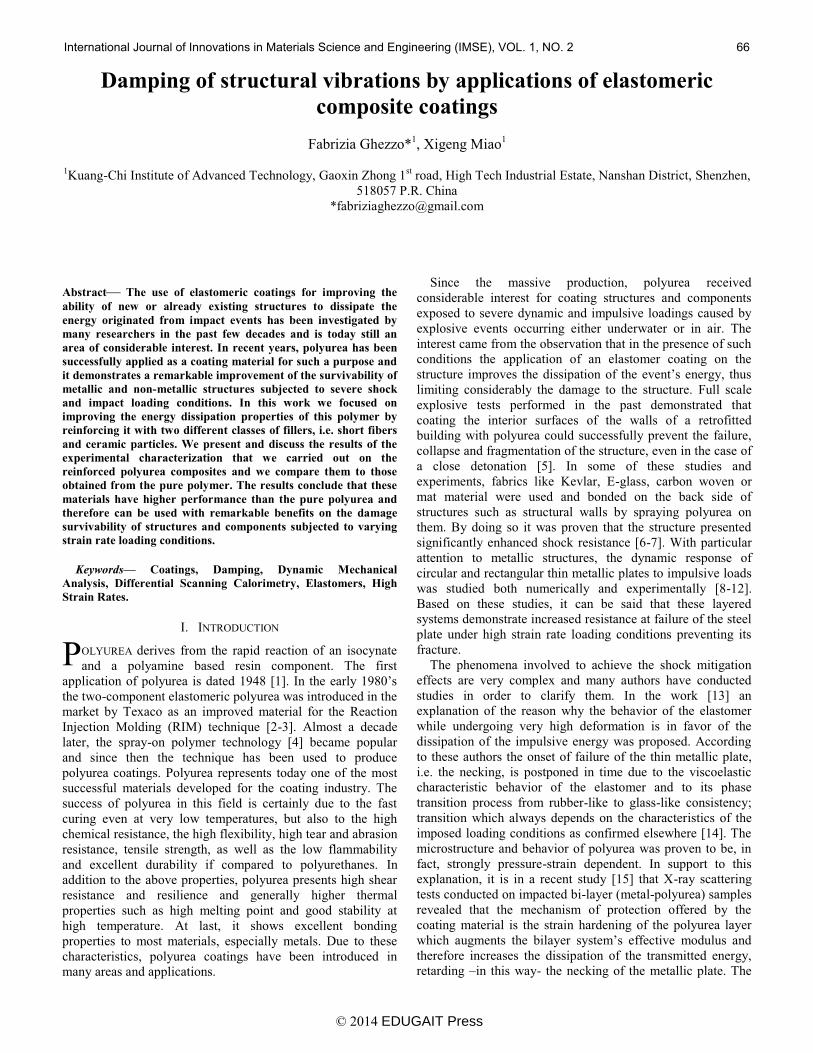
Damping of structural vibrations by applications of elastomeric
composite coatings
Fabrizia Ghezzo*1, Xigeng Miao
1
1Kuang-Chi Institute of Advanced Technology, Gaoxin Zhong 1
st road, High Tech Industrial Estate, Nanshan District, Shenzhen,
518057 P.R. China
Abstract The use of elastomeric coatings for improving the
ability of new or already existing structures to dissipate the
energy originated from impact events has been investigated by
many researchers in the past few decades and is today still an
area of considerable interest. In recent years, polyurea has been
successfully applied as a coating material for such a purpose and
it demonstrates a remarkable improvement of the survivability of
metallic and non-metallic structures subjected to severe shock
and impact loading conditions. In this work we focused on
improving the energy dissipation properties of this polymer by
reinforcing it with two different classes of fillers, i.e. short fibers
and ceramic particles. We present and discuss the results of the
experimental characterization that we carried out on the
reinforced polyurea composites and we compare them to those
obtained from the pure polymer. The results conclude that these
materials have higher performance than the pure polyurea and
therefore can be used with remarkable benefits on the damage
survivability of structures and components subjected to varying
strain rate loading conditions.
Keywords Coatings, Damping, Dynamic Mechanical
Analysis, Differential Scanning Calorimetry, Elastomers, High
Strain Rates.
I. INTRODUCTION
OLYUREA derives from the rapid reaction of an isocynate
and a polyamine based resin component. The first
the two-component elastomeric polyurea was introduced in the
market by Texaco as an improved material for the Reaction
Injection Molding (RIM) technique [2-3]. Almost a decade
later, the spray-on polymer technology [4] became popular
and since then the technique has been used to produce
polyurea coatings. Polyurea represents today one of the most
successful materials developed for the coating industry. The
success of polyurea in this field is certainly due to the fast
curing even at very low temperatures, but also to the high
chemical resistance, the high flexibility, high tear and abrasion
resistance, tensile strength, as well as the low flammability
and excellent durability if compared to polyurethanes. In
addition to the above properties, polyurea presents high shear
resistance and resilience and generally higher thermal
properties such as high melting point and good stability at
high temperature. At last, it shows excellent bonding
properties to most materials, especially metals. Due to these
characteristics, polyurea coatings have been introduced in
many areas and applications.
Since the massive production, polyurea received
considerable interest for coating structures and components
exposed to severe dynamic and impulsive loadings caused by
explosive events occurring either underwater or in air. The
interest came from the observation that in the presence of such
conditions the application of an elastomer coating on the
limiting considerably the damage to the structure. Full scale
explosive tests performed in the past demonstrated that
coating the interior surfaces of the walls of a retrofitted
building with polyurea could successfully prevent the failure,
collapse and fragmentation of the structure, even in the case of
a close detonation [5]. In some of these studies and
experiments, fabrics like Kevlar, E-glass, carbon woven or
mat material were used and bonded on the back side of
structures such as structural walls by spraying polyurea on
them. By doing so it was proven that the structure presented
significantly enhanced shock resistance [6-7]. With particular
attention to metallic structures, the dynamic response of
circular and rectangular thin metallic plates to impulsive loads
was studied both numerically and experimentally [8-12].
Based on these studies, it can be said that these layered
systems demonstrate increased resistance at failure of the steel
plate under high strain rate loading conditions preventing its
fracture.
The phenomena involved to achieve the shock mitigation
effects are very complex and many authors have conducted
studies in order to clarify them. In the work [13] an
explanation of the reason why the behavior of the elastomer
while undergoing very high deformation is in favor of the
dissipation of the impulsive energy was proposed. According
to these authors the onset of failure of the thin metallic plate,
i.e. the necking, is postponed in time due to the viscoelastic
characteristic behavior of the elastomer and to its phase
transition process from rubber-like to glass-like consistency;
transition which always depends on the characteristics of the
imposed loading conditions as confirmed elsewhere [14]. The
microstructure and behavior of polyurea was proven to be, in
fact, strongly pressure-strain dependent. In support to this
explanation, it is in a recent study [15] that X-ray scattering
tests conducted on impacted bi-layer (metal-polyurea) samples
revealed that the mechanism of protection offered by the
coating material is the strain hardening of the polyurea layer
therefore increases the dissipation of the transmitted energy,
retarding in this way- the necking of the metallic plate. The
P
© 2014 EDUGAIT Press
International Journal of Innovations in Materials Science and Engineering (IMSE), VOL. 1, NO. 2 66
authors were able to demonstrate that the hardening of the
polymer is in part - dependent on the process according to
which polyurea was made since the final molecular weights of
the hard and soft segments that compose the polymer
influence the response of the coating. At high strain rates of
impact, in fact, the hard and soft segments that compose the
polymer undergo a reformation and re-arrangement.
Specifically, it is reported that the hard domains break under
the high stress and reform in an oriented fiber form increasing
the strain hardening and thus increasing the impact resistance.
The nature of polyurea, composed by microphase soft domains
with partially crystalline hard segments [16-18], contributes to
the unique response of the material at high strain rate of
impact.
A number of studies were then carried out to quantify at
which extent stochiometric variations of the polymer
composition may influence its final mechanical properties.
Several authors investigated the change of the properties of
this polymer varying its composition [16-18] and also
characterized its viscoelastic behavior both experimentally and
numerically [13, 19-21]. Even though these contributions are
valuable to understand the response of this polymer at low
strain rates, it was observed that the resistance to ballistic
penetration is unaffected by stochiometric variations and with
regard to polyurea coatings for impact energy mitigation their
better performance requires radical changes in the structure
and morphology than those that can be achieved by
stochiometric variations [18].
The objective of this work was to improve substantially the
energy dissipation properties of polyurea under low or high
strain rate conditions. From previous works in this field, it can
be concluded that the response of the polymer at high strain
rate is very different from the one at lower strain rates, since
the transition from a rubbery to glassy state phenomena that
enhances the mitigation effects of the impact - only occurs at
high impact energies and at these conditions stochiometric
variations have no effects on the performance of the polymer.
It can be generally said that one way to improve the hardening
and toughening of the polymer and its overall mechanical
properties is by reinforcing it. Previous works on polyurea
with nano-fillers are already present in the literature [22-23],
however these works are not focusing on the effects of the
fillers on the behavior of the polymer at high strain rate. In a
study [24] target on the behavior of polyurea reinforced with
multi-wall carbon nanotubes (MWCN), nanoclay particles and
trisilanophenyl-functionalized polyhedral oligomeric
silsesquioxane (POSS) at high strain rates was presented. The
experimental observations enabled the authors to conclude that
no appreciable benefit on the performance at high rain rate can
be seen by reinforcing polyurea with nano-fillers. Previous
experimental work of the author [25-26] reported the
enhancement of the energy dissipation of the reinforced
polyurea coatings on metallic plates in impact events.
In this manuscript we report on the characterization of the
quasi static and dynamic properties of a poluyrea reinforced
with two different types of fillers. The improved ability of
dissipating energy presented by these materials was
demonstrated by comparing their quasi static and dynamic
behaviors with those of the pure elastomer. The
characterization of these materials was conducted in order to
support the conclusions made in previous experimental
observations where a few representative samples consisting of
thin metallic plates coated with reinforced polyurea were
subjected to high strain rate impact. The results demonstrated
that these materials might have increased the survivability of
the samples. As a consequence of those observations, a more
comprehensive characterization of the properties was
conducted on these materials. The evaluation of their dynamic
behavior was considered as a way to quantify and characterize
the damping ability of these materials as well as to verify the
presence of potential changes in the segmental dynamics [24].
Unlike the work [24] where the increase of the toughness of
polyurea was sought by adding nano-fillers which were then
proven to disrupt the segmental dynamics of the polymer with
no benefit to the performance of the material at high strain rate
impact, our addition of a micron-size reinforcement was
proved to have large benefit on increasing its overall
mechanical properties and also increasing remarkably the
survivability of the metallic component coated by such
materials at high strain rate impact (104
s-1
). Based on these
observations, we conclude that the optimization of the
performance of the polymer for the mitigation of the impact
energy is achieved by reinforcing it, but further studies are
necessary to understand the additional mechanisms that are
triggered in these composites when subjected to high strain
rate loading conditions.
II. MATERIALS AND EXPERIMENTAL PROCEDURE
A. Material and samples preparation
The polyurea used in this work was derived from the
combination of the following components: multifunctional
Isonate® 143L [28], and high molecular weight oligomeric
amine, Versalink® P1000 [29] in 1 to 4 proportions
respectively. In this study, polyurea was reinforced with two
types of fillers namely commercial milled E-glass fibers
kindly provided by Hebei Yuniu Fiberglass Manufacturing
Co., Ltd., with nominal fiber length of 0.3 mm and alumina
powder ceramic grade (99.7 % purity) with <1 m diameter
(typically of 0.3 m) from Zhengzhou Bihe Trade Co., Ldt.
P.R. China. All the materials were used as received. The
desired amount of fillers were first added to the blend resin
component and the mixture was stirred for 6 hours in a three-
neck round bottom reaction flask kept continuously under
vacuum in order to evacuate the air bubbles present in the
liquid. The isocynate component was degassed in a separate
glass flask, also under vacuum, and added to the rest of the
mixture at later time. After the addition of the isocynate, the
whole mixture was stirred for about 15 seconds before being
transferred into a teflon mould using a syringe. Once the
degassing procedure was finalized, the overall material
fabrication time required approximately 15 seconds for mixing
all the components together and extra 20 seconds for casting
the desired samples.
The samples consisted in un-confined quasi-static
compression and dynamic mechanical analysis samples.
Additional small specimens were used for scanning electron
microscopy (SEM). The quasi static compression samples
were obtained by pouring the mixed components into an open
Teflon mould where cylindrical cavities of 10 mm height and
International Journal of Innovations in Materials Science and Engineering (IMSE), VOL. 1, NO. 2 67
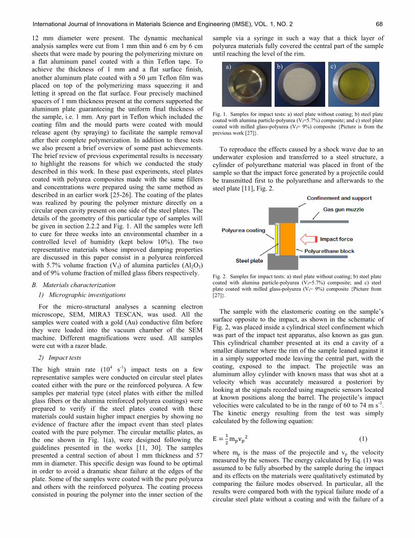
12 mm diameter were present. The dynamic mechanical
analysis samples were cut from 1 mm thin and 6 cm by 6 cm
sheets that were made by pouring the polymerizing mixture on
a flat aluminum panel coated with a thin Teflon tape. To
achieve the thickness of 1 mm and a flat surface finish,
another aluminum plate coated with a 50 m Teflon film was
placed on top of the polymerizing mass squeezing it and
letting it spread on the flat surface. Four precisely machined
spacers of 1 mm thickness present at the corners supported the
aluminum plate guaranteeing the uniform final thickness of
the sample, i.e. 1 mm. Any part in Teflon which included the
coating film and the mould parts were coated with mould
release agent (by spraying) to facilitate the sample removal
after their complete polymerization. In addition to these tests
we also present a brief overview of some past achievements.
The brief review of previous experimental results is necessary
to highlight the reasons for which we conducted the study
described in this work. In these past experiments, steel plates
coated with polyurea composites made with the same fillers
and concentrations were prepared using the same method as
described in an earlier work [25-26]. The coating of the plates
was realized by pouring the polymer mixture directly on a
circular open cavity present on one side of the steel plates. The
details of the geometry of this particular type of samples will
be given in section 2.2.2 and Fig. 1. All the samples were left
to cure for three weeks into an environmental chamber in a
controlled level of humidity (kept below 10%). The two
representative materials whose improved damping properties
are discussed in this paper consist in a polyurea reinforced
with 5.7% volume fraction (Vf) of alumina particles (Al2O3)
and of 9% volume fraction of milled glass fibers respectively.
B. Materials characterization
1) Micrographic investigations
For the micro-structural analyses a scanning electron
microscope, SEM, MIRA3 TESCAN, was used. All the
samples were coated with a gold (Au) conductive film before
they were loaded into the vacuum chamber of the SEM
machine. Different magnifications were used. All samples
were cut with a razor blade.
2) Impact tests
The high strain rate (104 s
-1) impact tests on a few
representative samples were conducted on circular steel plates
coated either with the pure or the reinforced polyurea. A few
samples per material type (steel plates with either the milled
glass fibers or the alumina reinforced polyurea coatings) were
prepared to verify if the steel plates coated with these
materials could sustain higher impact energies by showing no
evidence of fracture after the impact event than steel plates
coated with the pure polymer. The circular metallic plates, as
the one shown in Fig. 1(a), were designed following the
guidelines presented in the works [11, 30]. The samples
presented a central section of about 1 mm thickness and 57
mm in diameter. This specific design was found to be optimal
in order to avoid a dramatic shear failure at the edges of the
plate. Some of the samples were coated with the pure polyurea
and others with the reinforced polyurea. The coating process
consisted in pouring the polymer into the inner section of the
sample via a syringe in such a way that a thick layer of
polyurea materials fully covered the central part of the sample
until reaching the level of the rim.
To reproduce the effects caused by a shock wave due to an
underwater explosion and transferred to a steel structure, a
cylinder of polyurethane material was placed in front of the
sample so that the impact force generated by a projectile could
be transmitted first to the polyurethane and afterwards to the
steel plate [11], Fig. 2.
surface opposite to the impact, as shown in the schematic of
Fig. 2, was placed inside a cylindrical steel confinement which
was part of the impact test apparatus, also known as gas gun.
This cylindrical chamber presented at its end a cavity of a
smaller diameter where the rim of the sample leaned against it
in a simply supported mode leaving the central part, with the
coating, exposed to the impact. The projectile was an
aluminum alloy cylinder with known mass that was shot at a
velocity which was accurately measured a posteriori by
looking at the signals recorded using magnetic sensors located
velocities were calculated to be in the range of 60 to 74 m s-1
.
The kinetic energy resulting from the test was simply
calculated by the following equation:
(1)
where mp is the mass of the projectile and vp the velocity
measured by the sensors. The energy calculated by Eq. (1) was
assumed to be fully absorbed by the sample during the impact
and its effects on the materials were qualitatively estimated by
comparing the failure modes observed. In particular, all the
results were compared both with the typical failure mode of a
circular steel plate without a coating and with the failure of a
Fig. 2. Samples for impact tests: a) steel plate without coating; b) steel plate coated with alumina particle-polyurea (Vf=5.7%) composite; and c) steel
plate coated with milled glass-polyurea (Vf= 9%) composite Picture from
[27].
Fig. 1. Samples for impact tests: a) steel plate without coating; b) steel plate coated with alumina particle-polyurea (Vf=5.7%) composite; and c) steel plate
coated with milled glass-polyurea (Vf= 9%) composite Picture is from the
previous work [27].
a) b) c)
International Journal of Innovations in Materials Science and Engineering (IMSE), VOL. 1, NO. 2 68
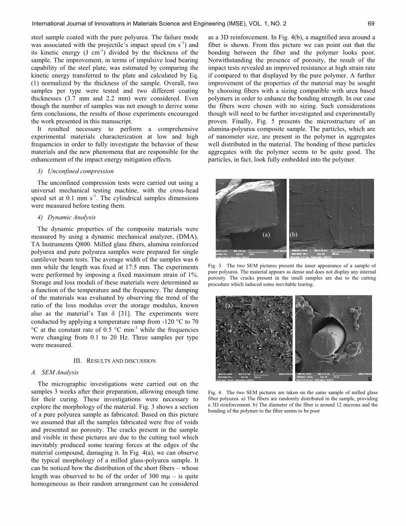
steel sample coated with the pure polyurea. The failure mode
was associated with t-1
) and
its kinetic energy (J cm-1
) divided by the thickness of the
sample. The improvement, in terms of impulsive load bearing
capability of the steel plate, was estimated by comparing the
kinetic energy transferred to the plate and calculated by Eq.
(1) normalized by the thickness of the sample. Overall, two
samples per type were tested and two different coating
thicknesses (3.7 mm and 2.2 mm) were considered. Even
though the number of samples was not enough to derive some
firm conclusions, the results of those experiments encouraged
the work presented in this manuscript.
It resulted necessary to perform a comprehensive
experimental materials characterization at low and high
frequencies in order to fully investigate the behavior of these
materials and the new phenomena that are responsible for the
enhancement of the impact energy mitigation effects.
3) Unconfined compression
The unconfined compression tests were carried out using a
universal mechanical testing machine, with the cross-head
speed set at 0.1 mm s-1
. The cylindrical samples dimensions
were measured before testing them.
4) Dynamic Analysis
The dynamic properties of the composite materials were
measured by using a dynamic mechanical analyzer, (DMA),
TA Instruments Q800. Milled glass fibers, alumina reinforced
polyurea and pure polyurea samples were prepared for single
cantilever beam tests. The average width of the samples was 6
mm while the length was fixed at 17.5 mm. The experiments
were performed by imposing a fixed maximum strain of 1%.
Storage and loss moduli of these materials were determined as
a function of the temperature and the frequency. The damping
of the materials was evaluated by observing the trend of the
ratio of the loss modulus over the storage modulus, known
[31]. The experiments were
conducted by applying a temperature ramp from -120 C to 70
C at the constant rate of 0.5 C min-1
while the frequencies
were changing from 0.1 to 20 Hz. Three samples per type
were measured.
III. RESULTS AND DISCUSSION
A. SEM Analysis
The micrographic investigations were carried out on the
samples 3 weeks after their preparation, allowing enough time
for their curing. These investigations were necessary to
explore the morphology of the material. Fig. 3 shows a section
of a pure polyurea sample as fabricated. Based on this picture
we assumed that all the samples fabricated were free of voids
and presented no porosity. The cracks present in the sample
and visible in these pictures are due to the cutting tool which
inevitably produced some tearing forces at the edges of the
material compound, damaging it. In Fig. 4(a), we can observe
the typical morphology of a milled glass-polyurea sample. It
can be noticed how the distribution of the short fibers whose
length was observed to be of the order of 300 m is quite
homogeneous as their random arrangement can be considered
as a 3D reinforcement. In Fig. 4(b), a magnified area around a
fiber is shown. From this picture we can point out that the
bonding between the fiber and the polymer looks poor.
Notwithstanding the presence of porosity, the result of the
impact tests revealed an improved resistance at high strain rate
if compared to that displayed by the pure polymer. A further
improvement of the properties of the material may be sought
by choosing fibers with a sizing compatible with urea based
polymers in order to enhance the bonding strength. In our case
the fibers were chosen with no sizing. Such considerations
though will need to be further investigated and experimentally
proven. Finally, Fig. 5 presents the microstructure of an
alumina-polyurea composite sample. The particles, which are
of nanometer size, are present in the polymer in aggregates
well distributed in the material. The bonding of these particles
aggregates with the polymer seems to be quite good. The
particles, in fact, look fully embedded into the polymer.
Fig. 4. The two SEM pictures are taken on the same sample of milled glass
fiber polyurea. a) The fibers are randomly distributed in the sample, providing
a 3D reinforcement. b) The diameter of the fiber is around 12 microns and the bonding of the polymer to the fiber seems to be poor
Fig. 3. The two SEM pictures present the inner appearance of a sample of
pure polyurea. The material appears as dense and does not display any internal porosity. The cracks present in the small samples are due to the cutting
procedure which induced some inevitable tearing.
(a) (b)
(a) (b)
International Journal of Innovations in Materials Science and Engineering (IMSE), VOL. 1, NO. 2 69

B. Impact tests
From the results of the impact tests it was first confirmed
that a layer of polyurea backing a steel plate impacted with the
same kinetic energy (per unit thickness) as the one that
induced a dramatic failure of a bare steel plate significantly
improved the absorption of the impact energy and, in all cases,
prevented the failure of the sample. It is necessary to observe
that the amount of fillers added to the polymer, is very small
to appreciate any consistent change of weight for the entire
sample as a consequence, inertia effects may be not claimed in
this work partly responsible for the introduction of the
improvements recorded during these tests. Said so, a dramatic
failure such as the one shown in Fig. 6(a) was attributed to
samples, with or without a coating, where a large central
opening was displayed after the impact. A moderate failure,
such as the one in Fig. 7(a), was attributed to those cases
where the steel plate after the impact was highly deformed and
presented evidence of cracks at the center.
No failure was instead attributed to those samples which
presented a large deformation but no evidence of cracks as
shown in Fig. 6(b), 6(c), 6(d) and Fig. 7(b). In Fig. 6(a), the
reference steel sample impacted with the kinetic energy of
15,347 J cm-1
62.18 m s-1
, displayed a severe failure, while the sample
coated with the milled glass fiber-polyurea shown in Fig. 6(b)
displayed high deformation but no fracture when impacted
with a energy level of 16,573.7 J cm-1
of 63.34 m s-1
.In this specific case, Fig. 6(b), in addition to the
improved impact resistance, the milled glass fiber-polyurea
composites demonstrated the unique ability of remaining
perfectly attached to the surface of the plate after the shock
event. The effect may find an explanation in the high
toughness that was observed to characterize this material, as
reported in the next section. The highest impact resistance was
displayed by samples coated with the alumina reinforced
polyurea. In fact, as shown in the Fig. 6(d) one of these
samples survived the impact after being shot with the energy
of 21,000 J cm-1
72.159 m s-1
. This was the highest impact energy recorded in
these experiments. No steel plate coated with the pure
polyurea or the milled glass fiber-polyurea survived at the
same impact energy. A comparison made with the failure of a
sample with the pure polyurea coating is presented in Fig. 7.
The plate coated with the pure polyurea, Fig. 7(a), presented a
moderate damage at impact energy of 17,945 J cm-1
and
m s-1
, while the plate coated with
the milled glass fiber polyurea, in Fig. 7(b), survived when
impacted with energy of 19,272 J cm-1
of 68.95 m s-1
. Once again, the reinforced polyurea coatings
seemed to increase the survivability at impact of these layered
systems.
Overall, the improvement in terms of impact resistance of
the samples was estimated to be 27% higher if compared to
tests conducted on bare steel plates and 15% higher with
respect to plates coated with the pure polyurea. The
improvement was observed to be consistent for samples with
two different coating thicknesses, i.e. 3.7 mm and 2.2 mm.
It can be argued that more experiments are necessary to
confirm the improvement and some of the results can be
questioned due to the small number of samples tested.
However, these encouraging results gave a qualitative idea of
the benefit that these materials may have over the pure
polymer and suggested a more comprehensive characterization
of the properties as presented in the following sections of this
manuscript. It is important to add that, in these earlier studies,
other types of reinforcement, such as flakes and longer fibers
(both of the order of 1 cm in size), was used but with no or
even negative effects on the performance of the coating at the
same strain rates of impact. The works on the microphase
composition of polyurea and the observations made on its
behavior [18] along with these experiments brought the
authors to assume that the hardening of the polymer through
Fig. 7. Two representative samples where the thickness of the coatings was
2.2 mm. a) Moderate failure of steel plate coated with pure polyurea atimpact energy of 17,945 J cm-1; b) milled glass-polyurea coating a steel plate
impacted with the energy 19,272 Jcm-1.
Fig. 6. Comparison of the impact results of some representative samples with 3.77 mm coating thickness: a) failure of steel plate S67 without coating at
15,347 J cm-1 as reported in previous experimental results [11]; b) milled
glass polyurea backing the steel plate MG249 impacted with the energy of 16,573.7 J cm-1; c) milled glass fiber polyurea coating the plate MG272
impacted with 20,805 J cm-1 energy; d) alumina reinforced polyurea coating
the plate AL271 impacted with 21000 J cm-1 energy Picture from [27].
Fig. 5. The picture shows the morphology of one alumina polyurea sample. It can be observed how the nano-particles are present in the material in larger
agglomerates. These agglomerates, however, seem to be homogenously
distributed in the material.
(a)
(a) (b) (c)
(c) (d)
(b)
(a) (b)
International Journal of Innovations in Materials Science and Engineering (IMSE), VOL. 1, NO. 2 70
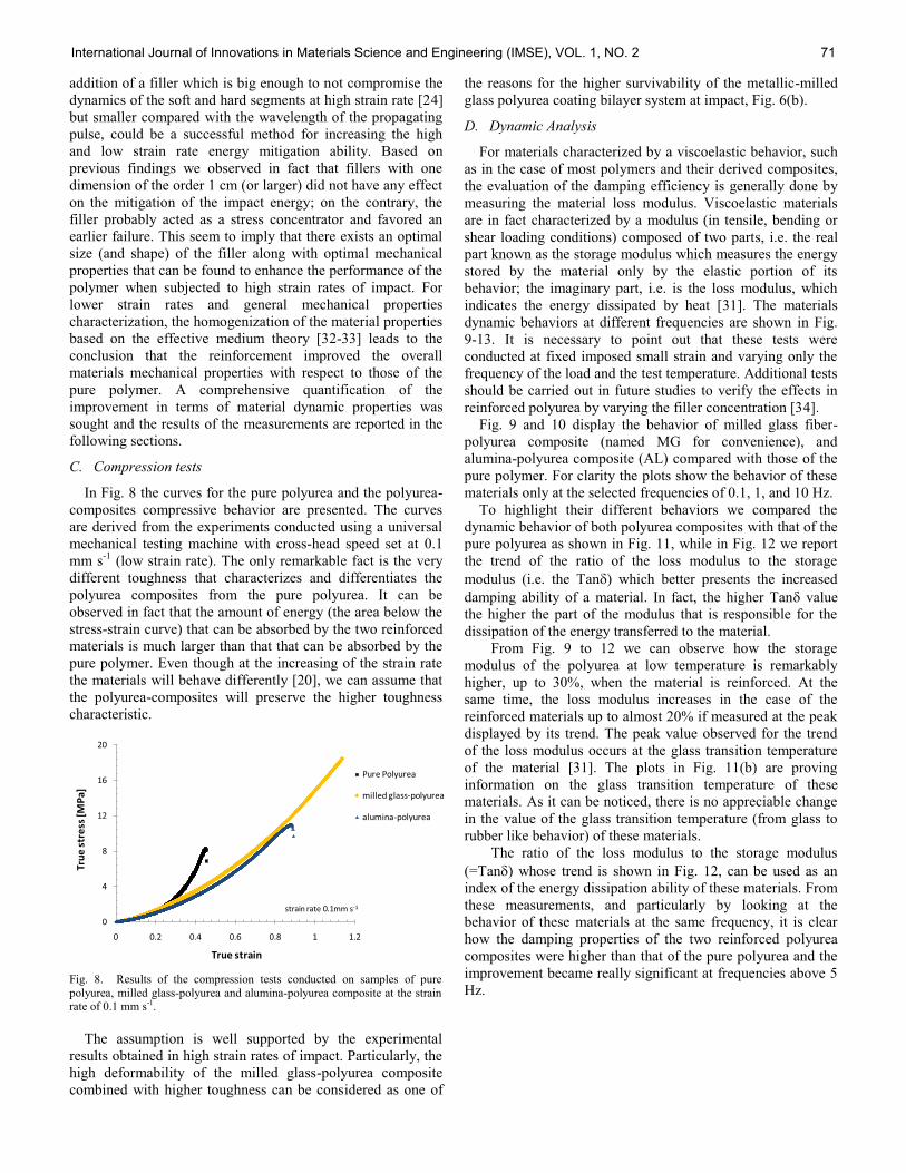
addition of a filler which is big enough to not compromise the
dynamics of the soft and hard segments at high strain rate [24]
but smaller compared with the wavelength of the propagating
pulse, could be a successful method for increasing the high
and low strain rate energy mitigation ability. Based on
previous findings we observed in fact that fillers with one
dimension of the order 1 cm (or larger) did not have any effect
on the mitigation of the impact energy; on the contrary, the
filler probably acted as a stress concentrator and favored an
earlier failure. This seem to imply that there exists an optimal
size (and shape) of the filler along with optimal mechanical
properties that can be found to enhance the performance of the
polymer when subjected to high strain rates of impact. For
lower strain rates and general mechanical properties
characterization, the homogenization of the material properties
based on the effective medium theory [32-33] leads to the
conclusion that the reinforcement improved the overall
materials mechanical properties with respect to those of the
pure polymer. A comprehensive quantification of the
improvement in terms of material dynamic properties was
sought and the results of the measurements are reported in the
following sections.
C. Compression tests
In Fig. 8 the curves for the pure polyurea and the polyurea-
composites compressive behavior are presented. The curves
are derived from the experiments conducted using a universal
mechanical testing machine with cross-head speed set at 0.1
mm s-1
(low strain rate). The only remarkable fact is the very
different toughness that characterizes and differentiates the
polyurea composites from the pure polyurea. It can be
observed in fact that the amount of energy (the area below the
stress-strain curve) that can be absorbed by the two reinforced
materials is much larger than that that can be absorbed by the
pure polymer. Even though at the increasing of the strain rate
the materials will behave differently [20], we can assume that
the polyurea-composites will preserve the higher toughness
characteristic.
The assumption is well supported by the experimental
results obtained in high strain rates of impact. Particularly, the
high deformability of the milled glass-polyurea composite
combined with higher toughness can be considered as one of
the reasons for the higher survivability of the metallic-milled
glass polyurea coating bilayer system at impact, Fig. 6(b).
D. Dynamic Analysis
For materials characterized by a viscoelastic behavior, such
as in the case of most polymers and their derived composites,
the evaluation of the damping efficiency is generally done by
measuring the material loss modulus. Viscoelastic materials
are in fact characterized by a modulus (in tensile, bending or
shear loading conditions) composed of two parts, i.e. the real
part known as the storage modulus which measures the energy
stored by the material only by the elastic portion of its
behavior; the imaginary part, i.e. is the loss modulus, which
indicates the energy dissipated by heat [31]. The materials
dynamic behaviors at different frequencies are shown in Fig.
9-13. It is necessary to point out that these tests were
conducted at fixed imposed small strain and varying only the
frequency of the load and the test temperature. Additional tests
should be carried out in future studies to verify the effects in
reinforced polyurea by varying the filler concentration [34].
Fig. 9 and 10 display the behavior of milled glass fiber-
polyurea composite (named MG for convenience), and
alumina-polyurea composite (AL) compared with those of the
pure polymer. For clarity the plots show the behavior of these
materials only at the selected frequencies of 0.1, 1, and 10 Hz.
To highlight their different behaviors we compared the
dynamic behavior of both polyurea composites with that of the
pure polyurea as shown in Fig. 11, while in Fig. 12 we report
the trend of the ratio of the loss modulus to the storage
modulus (i.e. the Tan ) which better presents the increased
damping ability of a material. In fact, the higher Tan value
the higher the part of the modulus that is responsible for the
dissipation of the energy transferred to the material.
From Fig. 9 to 12 we can observe how the storage
modulus of the polyurea at low temperature is remarkably
higher, up to 30%, when the material is reinforced. At the
same time, the loss modulus increases in the case of the
reinforced materials up to almost 20% if measured at the peak
displayed by its trend. The peak value observed for the trend
of the loss modulus occurs at the glass transition temperature
of the material [31]. The plots in Fig. 11(b) are proving
information on the glass transition temperature of these
materials. As it can be noticed, there is no appreciable change
in the value of the glass transition temperature (from glass to
rubber like behavior) of these materials.
The ratio of the loss modulus to the storage modulus
(=Tan ) whose trend is shown in Fig. 12, can be used as an
index of the energy dissipation ability of these materials. From
these measurements, and particularly by looking at the
behavior of these materials at the same frequency, it is clear
how the damping properties of the two reinforced polyurea
composites were higher than that of the pure polyurea and the
improvement became really significant at frequencies above 5
Hz.
0
4
8
12
16
20
0 0.2 0.4 0.6 0.8 1 1.2
Pure Polyurea
milled glass-polyurea
alumina-polyurea
Tru
e s
tre
ss [
MP
a]
True strain
strain rate 0.1mm s-1
Fig. 8. Results of the compression tests conducted on samples of pure
polyurea, milled glass-polyurea and alumina-polyurea composite at the strain rate of 0.1 mm s-1.
International Journal of Innovations in Materials Science and Engineering (IMSE), VOL. 1, NO. 2 71

Fig. 9. Results of the dynamic mechanical analyses: a) storage modulus and b) loss modulus of pure polyurea (PU) compared with those of the milled glass fiber reinforced polyurea (MG), plotted at the selected frequencies of 0.1, 1 and 10 Hz.
Fig. 10. Results of the dynamic mechanical analyses: a) storage modulus and b) loss modulus of polyurea (PU) compared with those of alumina-
polyurea composite (AL) plotted at the selected frequencies of 0.1, 1 and 10 Hz.
Fig. 11. Dynamic properties of the reinforced polyurea compared with the pure polyurea: a) storage modulus and b) loss modulus of polyurea (PU),
milled glass-polyurea (MG) and alumina-polyurea composite (AL), plotted at the selected frequencies of 0.1 and 1 Hz for clarity.
0
500
1000
1500
2000
2500
3000
3500
4000
4500
-140 -120 -100 -80 -60 -40 -20 0 20 40 60 80
Sto
rag
e M
od
ulu
s [
MP
a]
Temperature C
SM PU 0.1 Hz
SM PU 1 Hz
SM Pu 10 Hz
SM MG 0.1 Hz
SM MG 1 Hz
SM MG 10 Hz
0
50
100
150
200
250
300
-140 -120 -100 -80 -60 -40 -20 0 20 40 60 80
Lo
ss
Mo
du
lus
[M
Pa
]
Temperature °C
LM PU 0.1 Hz
LM PU 1 Hz
LM PU 10 Hz
LM MG 0.1 Hz
LM MG 1 Hz
LM MG 10 Hz
0
500
1000
1500
2000
2500
3000
3500
4000
4500
-140 -120 -100 -80 -60 -40 -20 0 20 40 60 80
Sto
rag
e M
od
ulu
s [
MP
a]
Temperature °C
SM PU 0.1 Hz
SM PU 1 Hz
SM PU 10 Hz
SM AL 0.1 Hz
SM AL 1 Hz
SM AL 10 Hz
a)
0
50
100
150
200
250
-140 -120 -100 -80 -60 -40 -20 0 20 40 60 80
Lo
ss
Mo
du
lus [
MP
a]
Temperature °C
LM PU 0.1 Hz
LM PU 1 Hz
LM PU 10 Hz
LM AL 0.1 Hz
LM AL 1 Hz
LM AL 10 Hz
b)
0
500
1000
1500
2000
2500
3000
3500
4000
-140 -120 -100 -80 -60 -40 -20 0 20 40 60 80
Sto
rag
e M
od
ulu
s [
MP
a]
Temperature °C
SM PU 0.1 Hz
SM PU 1 Hz
SM MG 0.1 Hz
SM MG 1 Hz
SM AL 0.1 Hz
SM AL 1 Hz
a)
0
50
100
150
200
250
-140 -120 -100 -80 -60 -40 -20 0 20 40 60 80
Lo
ss
Mo
du
lus [
MP
a]
Temperature °C
LM PU 0.1 Hz
LM PU 1 Hz
LM MG 0.1 Hz
LM MG 1 Hz
LM AL 0.1 Hz
LM AL 1 Hz
b)
a) b)
International Journal of Innovations in Materials Science and Engineering (IMSE), VOL. 1, NO. 2 72

By considering the storage modulus, it is also evident how
the strength of these composite materials increased
substantially (in the range of 30%) if compared with that of
the pure polyurea. We can therefore conclude that the dynamic
response of the polyurea coatings subjected to high frequency
pulses, like a shock impulse caused by a close detonation
underwater, may be improved by using a polyurea coating
resulting from the addition of a proper amount and type of
filler. In fact, the heterogeneity of the microstructure and the
toughening of the material by addition of the filler not only is
in favor of the high dissipation abilities at low strain rates but
may be also in favor of the higher energy mitigation effects
occurring at high strain rates, supporting the results obtained
from the impact tests.
IV. CONCLUSIONS
The behavior at high strain rates of impact and the quasi
static and dynamic characterization at low frequency and low
strain rates of a reinforced polyurea elastomer were presented
in this work. Specifically, the improved damping properties of
the polyurea were obtained by reinforcing the polymer with
milled glass fibers and alumina particles. In a previous
experimental investigation, a few steel samples coated with
the pure polyurea and with the reinforced polyurea were
impacted by a projectile whose speed was in the range of 60 to
75 m s-1
. From the observations made on the failure modes of
the bi-layer system (steel plates and polyurea coatings)
subjected to impact we concluded that when a thin layer of the
reinforced polyurea material was backing a steel plate and the
plate was then impacted with the same kinetic energy (per unit
thickness) as the one that induced a dramatic failure of a steel
plate coated with the pure polyurea, the plate presented a high
deformation but did not fail. The explanation of these results
was given by assuming that the energy dissipation ability of
the material increased considerably by adding the fillers. The
confirmation of this assumption was obtained by
characterizing the dynamic properties of these materials. From
the presented experimental study we can extract some
important conclusions:
The compression behavior of these materials shows that
the polyurea composites are characterized by much higher
toughness. This property, i.e. the ability of the material to
store the energy before failure, is in support of the
observed beneficial effects on the increase ability of
mitigating the impact energy. These materials in fact
display higher deformation ability, characteristic which
was observed during the impact tests.
The loss and storage moduli of milled glass fibers and
alumina-polyurea composites are generally higher than that
of the pure polyurea. The increase is remarkable at low
temperature and particularly close to the glass transition
region but the improvement can be clearly noticed also at
temperatures above 20 C. The dynamic behavior of the
loss modulus characterizes the viscoelastic behavior of the
material and indicates the ability of the material to
dissipate energy. The property increases with the increase
of the frequency of the applied load. These observations
are also proving the better performance recorded at impact.
The glass transition temperature of the reinforced polyurea
composites, as shown by the trend of the loss modulus,
does not change from that of pure polyurea. This means
that the fillers in our case - seem to not disrupt the
polymer soft and hard domain composition as noticed in
previous works present in the literature.
The morphology of the polyurea composites, as from the
scanning electron microscopy analysis (SEM), shows that
milled glass fibers-polyurea composite are characterized by
a presence of distributed micro-porosity due to a poor
bonding between the fiber and the matrix while alumina-
composites are dense and the particles are fully embedded
into the matrix. These two different morphologies are both
helpful to explain the improved - but different - behavior of
these materials at impact. The presence of a poor bonding
between the fibers and the polymer in the former case,
favors the higher energy dissipation at impact by triggering
additional friction phenomena. The latter case instead, the
presence of a well bonded ceramic filler hardens the matrix
and allows the polymer to sustain much higher impact
force, as verified by conducting the experiments.
To conclude, it is possible to increase substantially the
impact energy mitigation ability of the polyurea coatings by
addition of fillers. Fillers of different type imply different
micro-mechanical and dynamic behavior at impact. Inclusions
larger than a nanometer size seem to not disrupt the segmental
dynamics of the polymer and, instead, add extra internal
dissipation phenomena or hardening at the benefit of the
increased survivability of the system. In order to optimize the
behavior of these materials, further studies and experiments
are needed for the full understanding of the phenomena
involved. We also think that an optimal response can be
achieved by the material if the range of frequency of the
impact event is known (or can be predicted). In such a way the
having a maximum at such a frequency or in a range of
frequencies close to that of an event concerned.
0
0.05
0.1
0.15
0.2
0.25
-140 -120 -100 -80 -60 -40 -20 0 20 40 60 80
Ta
n
Temperature °C
PU 0.1 Hz
PU 10Hz
MG 0.1Hz
MG 10Hz
Al 0.1Hz
Al 10Hz
Fig. 12. Tan of the milled glass fiber and alumina polyurea composites
compared with those of the pure polyurea at the selected frequencies of 0.1 and 10 Hz.
International Journal of Innovations in Materials Science and Engineering (IMSE), VOL. 1, NO. 2 73
ACKNOWLEDGMENT
This work was partially supported by the Shenzhen Innovative
R&D Team Program (Peacock plan), No.
KQE201106020031A.
REFERENCES
[1] R. Hill, and E.E. Walker, Polymer Constitution and Fiber properties,
J. Polym. Sci., vol. 3, no. 5, pp. 609-630, 1948. [2] R.A. Grigsby Jr., and D.M. Rice, Some recent advances in Polyurea
RIM, J. Cell. Plast, vol. 22, pp. 484-495, 1986.
[3] F. Sann Jr., Improved RIM polyurea body panels, J. Cell. Plast., vol. 28, pp. 14-23, 1992.
[4] J. Primeaux Dudley, Spray polyurea elastomer using chopped glass
roving, U.S. Patent 5118728, Jun 2, 1992. [5] K.J. Knox, M.I. Hammons, T.T. Lewis, and J.R. Porter, Polymer
Materials for Structural Retrofit, Force protection branch, Air
Expeditionary Forces Technologies Division, Air Force Research Laboratory, technical report, Tyndall AFB, Florida, 2000.
[6] J.E. Crawford, Modeling blast-resistant protection systems composed
of polymers and fabric, Karagozian & Case, technical report. [7] J.E. Crawford, and L. Shengrui, Design and implementation of
protective technologies for improving blast resistance of buildings,
Enhancing Building Security Seminar, Singapore, 2005. [8] G.N. Nurick, and J.B. Martin, Deformation of thin plates subjected to
impulsive loading-A review, Part I: theoretical considerations, Int. J.
Impact Eng., vol. 8, no. 2, pp. 159-170, 1989. [9] G.N. Nurick, and J.B. Martin, Deformation of thin plates subjected to
impulsive loading-A review, Part II: Experimental Studies, Int. J.
Impact Eng., vol. 8, no. 2, pp. 171-186, 1989. [10] W. Mock, and E. Balizer, paper presented at Polyurea Properties and
Enhancement of Structures under Dynamics loads Airlie, VA, 2005.
[11] M.R. Amini, Effect of Polyurea on the dynamic response and fracture resistance of steel plates under impulsive loads, PhD Dissertation,
Dept. Mech. Aero. Eng., Uni. California San Diego, 2007.
[12] Z. Xue, and J.W. Hutchinson, Neck retardation and enhanced energy absorption in metal-elastomer bilayers, Mech. Mater., vol. 39, pp. 473-
487, 2007.
[13] J. Yi, M.C. Boyce, G.F. Lee, and E. Balizer, Large deformation rate-dependent stress-strain behavior of polyurea and polyurethanes,
Polymer, vol. 47, pp. 319-329, 2006.
[14] R.B. Bogoslovov, C.M. Roland, and R.M. Gamache, Impact-induced glass transition in elastomeric coatings, Appl. Phys. Lett., vol. 90,
221910-3, 2007.
[15] E. Balizer, J. Fedderly, Gilber Lee, S. Bartyczak, and W. Mock Jr., Investigation of microstructural changes in impacted polyurea coatings
using small angle X-ray scattering (SAXS), Powder Diffraction, vol.
26, no. 2, pp. 149-154, 2010. [16] W. R. Willkomm, Z.S. Chen, C. W. Macosko, D.A. Gobran, and E.L.
Thomas, Properties and phase separation of reaction injection molded
and solution polymerized polyureas as a function of hard block content, Polym. Eng. Sci., vol. 28, no. 14, pp. 888-900, 1988.
[17] A. J. Ryan, J.L. Stanford, and A.N. Wilkinson, Structure properties relations in non-linear segmented copolyureas formed by reaction
Polym. Bull., vol. 18, pp. 517-523, 1987.
[18] D. Fragiadakis, R. Gamache, R.B. Bogoslovov, and C.M. Roland, Segmental dynamics of polyurea, effect of stoichiometry, Polymer,
vol. 51, pp. 178-184, 2010.
[19] C.M. Roland, J.N. Twigg, Y. Vu, and P.H. Mott, High strain rate mechanical behavior of polyurea, Polymer, vol. 48, pp. 574-578,
2007.
[20] C.M. Roland, and R. Casalini, Effect of hydrostatic pressure on the viscoelastic r Polymer, vol. 48, no. 18, pp. 5747-
5752, 2007.
[21] A.V. Amirkhizi, J. Isaacs, J. McGee, and S. Nemat-Nasser, An experimentally-based viscoelastic constitutive model for polyurea,
including pressure and temperature effects, Philos. Magazine, vol. 86,
no. 36, pp. 5847-5866, 2006. [22] W. Awad, and C. Wilkie, Investigation of the thermal degradation of
polyurea: the effect of ammonium polyphosphate and expandable
graphite, Polymer, vol. 51, no. 11, 2010. [23] X. Qian, B. Yu, C. Bao, L. Song, B. Wang, W. Xing, Y. Hu, and R.K.K
Yuen, Silicon nanoparticles decorated graphene composites:
preparation and their reinforcement on the fire safety and mechanical
properties of polyurea, J. Mater. Chem. A, vol. 1, pp. 9827-9836, 2013. [24] R. Casalini, R. Bogoslovov, S.B. Qadri, and C.M. Roland, Nanofiller
reinforcement of elastomeric polyurea, Polymer, 53, pp. 1282-1287,
2012. [25] F. Ghezzo, A. V. Amirkhizi, S. Nemat-
iled
document UCSD Docket no SD2008-021; Remained unpublished. [26] F. Ghezzo, Materials with integrated distributed sensing,
the Cellular Concepts for the mitigation of localized high intensity
dynamic loads Conference, University of California Santa Barbara, Mar. 26-28, 2008.
[27] F. Ghezzo, and X. Miao, Composite coatings with high vibration
damping properties, presented at the 11th International Conference on Vibration Problems, ICOVP, Lisbon, Portugal, 9-12 Sept., 2013.
[28] Isonate® 143L, the Dow Chemical Company, Modified MDI, 2001,
Midland. [29] Versalink P1000, Air Products and Chemicals, Inc., 2003, Allentown,
PA.
[30] S. Nemat-Nasser, J.B. Isaacs, Hopkinson techniques for dynamic recovery experiments, Proc. R. Soc. A, vol. 435, pp. 371-
391, 1991.
[31] J.D. Ferry, Viscoelastic properties of polymers. 3rd Edition: Wiley, 1980.
[32] M.S. Jhon, R.J. Metz, and K.F. Freed, Effective medium theory for
elastic matrix composites containing dispersed particulates, J. Stat. Phys., vol. 52, no. 5/6, pp. 1325-1342, 1988.
[33] L.E. Nelson, Mechanical properties of Polymers and Composites. New York: Marcel Dekker, 1974
[34]
particle size and polymer-filler coupling on vicoelastic glass transition of particle- Macromolecules, vol. 41, pp. 2727-
2731, 2008.
International Journal of Innovations in Materials Science and Engineering (IMSE), VOL. 1, NO. 2 74
JOURNAL OF VOL. X, NO. X, MONTH X, 2014 1
Negative Stiffness Materials for Vibration Damping: a Material
Realization of a Nonlinear Bistable Element
Jan Heczko1, Zuzana Dimitrovová*
2, Hélder C. Rodrigues
3
1Department of Mechanics, Faculty of Applied Sciences, University of West Bohemia, Pilsen
2Departamento de Engenharia Civil, Faculdade de Ciências e Tecnologia, Universidade Nova de Lisboa and LAETA, IDMEC,
Instituto Superior Técnico, Universidade de Lisboa, Lisboa, Portugal 3LAETA, IDMEC, Instituto Superior Técnico, Universidade de Lisboa, Lisboa, Portugal
Abstract This paper addresses material and shape design of
a prototype exhibiting a negative stiffness over a finite range of
global strains. The objective is to define a design loop, where,
starting from the actual material realization, a corresponding
finite element model is developed and associated to a bistable
discrete one-dimensional mechanical system composed of pre-
compressed springs, a stabilizing spring and a damper. The
discrete model can easily be analyzed and optimized for
improved vibration damping properties. This will allow the
determination of an alternative specification of a new optimized
prototype. If confirmed by finite element analysis, then an
improved prototype can be produced accordingly. This paper
presents the first results: the material realization and the
corresponding discrete model identification exploring also the
finite element model. Optimization will be subject of further
research. It is concluded that the specimen behaves according to
the expectations, i.e. the negative stiffness region is well-formed
and the discrete correspondence is easily obtainable. Such a
structure can be used as a negative-stiffness element to achieve
extreme mechanical properties of a composite or as a structure
with improved damping properties.
Keywords Experimental Testing, Finite Element Modelling,
Negative Stiffness, Nonlinear Bistable Element, Vibration
control.
I. INTRODUCTION
RECENT PROGRESS in material processing and
manufacturing has stimulated strong scientific and
industrial interest in material design optimization. Tailoring
material properties to achieve the optimal response to a given
solicitation provides an important input to the development of
new materials. New horizons in novel materials can be opened
if the concept of the structural negative stiffness is considered.
Materials with adequate mixtures of carefully selected
phases, including also a negative stiffness phase, have been
shown to possess the ability of reaching extreme properties,
such as stiffness or vibration damping [1, 2]. Apart from many
studies exploring theoretically advances achieved in materials
incorporating negative stiffness constituents [3] there are also
real world applications that had proven utility of this concept.
Attempts to manufacture such materials were made using
unstable structures [4, 5], which exhibit negative stiffness in
the vicinity of the unstable equilibrium point. In this case one
has to constrain the negative stiffness components in order to
ensure that the structure really operates smoothly along the
negative branch of the force-displacement graph and does not
jump into one of the stable states.
Negative stiffness dampers are already available on the
article [7], Minus K Technology [8], founded in 1993 by Dr.
Platus, is the leading industry manufacturing negative stiffness
dampers. Nevertheless, advantages of such mechanisms were
already documented in Russian monograph that was later on
translated to English [9]. One of the most recent alternative
realizations is given in [10]. In [10] pre-compressed beams
represent the negative stiffness component that is stabilized by
another spring. The specimen was produced by 3D systems
Sinter station Hi QTM
selective laser sintering machine. It was
proven that with the increasing pre-compression, implying
decrease in fundamental frequency, also the decrease in
resonance peak in displacement transmissibility is verified.
Nevertheless, it is still a challenging task to design a
continuous isotropic three-dimensional material, easy to
manufacture, that would globally act in the same way as a
discrete mechanism.
In this paper a material produced from polyethylene foam
sheets is examined. Such a material is often used for packing
protection and it is known for its several other useful
properties like easy forming and possibility of heat-welding.
In order to integrate an inherent bistable element in such
sheets, additional semi-circumferential cuts were introduced.
The advantage of this realization is that the material, apart
from additional cuts, does not need any special manufacturing
technique as the one described in [10]. The base material is
easily accessible and cheap. The work presented here is an
extension of the preliminary results published in [11], which
was developed in continuation with [12].
The new contribution of this paper consists in the innovative
realization of a material exhibiting negative stiffness over a
range of finite strains and in the development of a method that
links this material with a discrete mechanism exploiting also
the finite element model. Future work will address its
performance optimization.
The paper is organized in the following way. In Section II
the polyethylene foam material is described and results of
experimental tests are given. In Section III finite element
model is developed and numerical results are presented and
compared with the experimental testing. A procedure of
R
International Journal of Innovations in Materials Science and Engineering (IMSE), VOL. 1, NO. 2 75
© 2014 EDUGAIT Press
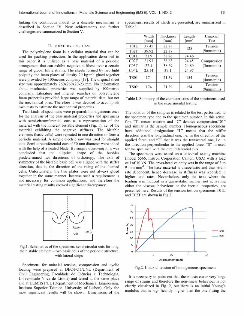
JOURNAL OF VOL. X, NO. X, MONTH X, 2014 2
linking the continuous model to a discrete mechanism is
described in Section IV. New achievements and further
challenges are summarized in Section V.
II. POLYETHYLENE FOAM
The polyethylene foam is a cellular material that can be
used for packing protection. In the application described in
this paper it is utilized as a base material of a periodic
arrangement that can exhibit negative stiffness over a certain
range of global finite strains. The sheets formed by two light
polyethylene foam plates of density 20 kg·m-3
glued together
were provided by 100metros company [13]. The original sheet
size was approximately 260x260x20-23 mm. No information
about mechanical properties was supplied by 100metros
company. Literature and internet searches on polyethylene
foam properties provided large range of material data, but not
the mechanical ones. Therefore it was decided to accomplish
own tests to estimate the mechanical properties.
Two kinds of specimens were prepared: homogeneous ones
for the analysis of the base material properties and specimens
with semi-circumferential cuts as a representation of the
material with the inherent bistable element (Fig. 1), i.e. of the
material exhibiting the negative stiffness. The bistable
elements (basic cells) were repeated in one direction to form a
periodic material. A simple electric saw was used for straight
cuts. Semi-circumferential cuts of 50 mm diameter were added
with the help of a heated blade. By simply observing it, it was
concluded that the elliptical shape of the bubbles
predetermined two directions of orthotropy. The axis of
symmetry of the bistable basic cell was aligned with the stiffer
direction, that is, the direction of the rising of the foamed
cells. Unfortunately, the two plates were not always glued
together in the same manner, because such a requirement is
not necessary for common applications, and therefore the
material testing results showed significant discrepancy.
Fig.1. Schematics of the specimen: semi-circular cuts forming
the bistable element two basic cells of the periodic structure
with lateral strips
Specimens for uniaxial tension, compression and cyclic
loading were prepared at DEC/FCT/UNL (Department of
Civil Engineering, Faculdade de Ciências e Technologia,
Universidade Nova de Lisboa) and tested at the same place
and at DEM/IST/UL (Department of Mechanical Engineering,
Instituto Superior Técnico, University of Lisbon). Only the
most significant results will be shown. Dimensions of the
specimens, results of which are presented, are summarized in
Table I.
Width
[mm]
Thickness
[mm]
Length
[mm]
Uniaxial
Test
T01L 37.45 22.78 125
Tension
(9mm/min) T02T 39.92 22.38
C01L 21.9 38.26 24.46
Compression
(3mm/min)
C02T 21.93 38.63 24.45
C03T 22.1 38.69 24.89
C04L 25.14 39.1 24.97
TS01 174 21.39 154 Tension
(4mm/min)
TS02 174 21.39 154 Tension
(9mm/min)
Table I. Summary of the characteristics of the specimens used
in the experimental testing
The notation of the samples is related to the test performed, to
the specimen type and to the specimen number. In this sense,
and similar is the sample number. Homogeneous specimens
that the stiffer
direction was the longitudinal one, i.e. in the direction of the
the transversal one, i.e. in
for the specimen with the circumferential cuts.
The specimens were tested on a universal testing machine
(model 5566, Instron Corporation Canton, USA) with a load
cell of 10 kN. The cross-head velocity was in the range of 3 to
9 mm·min-1
. The base material is viscoelastic and thus strain
rate dependent, hence decrease in stiffness was recorded in
higher load rates. Nevertheless, only the tests where the
loading was induced in a quasi-static manner, not activating
either the viscous behaviour or the inertial properties, are
presented here. Results of the tension test on specimens T01L
and T02T are shown in Fig.2.
Fig.2. Uniaxial tension of homogeneous specimens
It is necessary to point out that these tests cover very large
range of strains and therefore the non-linear behaviour is not
modulus that is significantly higher than the one fitting the
stripbasic
cell
International Journal of Innovations in Materials Science and Engineering (IMSE), VOL. 1, NO. 2 76

JOURNAL OF VOL. X, NO. X, MONTH X, 2014 3
most of the force-displacement curve. In Fig. 3 secant
modulus is plotted in each force increment and overlaid by a
trend line obtained by a moving averaging method of rank 4.
Fig.3. Secant modulus and trend lines obtained by a moving
average method related to the initial part of the force-
displacement curve from Fig. 2
Regarding the stiffer direction, the elastic modulus
decreases exponentially from the initial value of 3 MPa to 1.6
MPa at approximately 0.008 engineering strain and then it
drops to 1 MPa at 0.02 engineering strain. Regarding the
softer direction, the modulus starts at 0.5 MPa, slowly
decreases to 0.4MPa and the specimen is able to bear very
large engineering strains, reaching 0.1, when the modulus
starts to decrease again. As expected, the behaviour in
compression is quite different and the elastic moduli are
significantly lower. Experimental curves are shown in Fig. 4.
Fig.4. Uniaxial compression of homogeneous specimens
It is seen that for the longitudinal direction the strength is
higher in compression than in tension, but the stiffness is
significantly lower. There is also a significant difference in
longitudinal and transversal directions. Roughly speaking, the
stiffness ratio between the stiffer and the softer direction
around 4. Moduli in transversal direction do not show
significant difference when related to tension and
compression, but in longitudinal direction the ratio of tension
and compression modulus is around 20.
Furthermore, the bistable structure was tested. As expected,
one basic cell of the bistable material was not sufficient to
provide the required behaviour, because there was insufficient
lateral constraint, and therefore the specimen was unable to
show the negative branch in the global stiffness. These results
will not be shown here. Specimens with two basic cells and
lateral strips (Fig.1.) were tested instead. The lateral strip
provided necessary constraint and facilitated a smooth snap
through the unstable equilibrium. Two displacement rates
were implemented as 4 mm·min-1
and 9 mm·min-1
, but no
significant differences were found between the results.
Different phases of the loading are shown in Fig. 5, the
negative branch is verified between stages (b) and (c).
Fig. 5. Tension test on the bistable material: (a) initial
position, (b) beginning of the negative stiffness, (c) new
beginning of the positive stiffness, (d) initiation of failure
Monotonic displacement-control tests revealed that the
negative stiffness region in force-displacement curve is well-
formed. However, a visible out-of-plane deformation helped to
reach the next stable equilibrium at lower global force, than it
would be required by a perfectly plane specimen. Fortunately
this fact did not affect the global performance, but in future
works some preventive measures have to be taken, like for
instance reinforce the specimen by a stiffer thin plate that
would prevent out-of plane deformations. The force-
)d)c
)b)a
International Journal of Innovations in Materials Science and Engineering (IMSE), VOL. 1, NO. 2 77

JOURNAL OF VOL. X, NO. X, MONTH X, 2014 4
displacement curves related to the experiment described above
are shown in Fig. 6.
Fig.6. Tension tests on the bistable material
In Fig.6 caption - - number of the
test performed on the same specimen TS02. Specimen TS01
was left until the failure.
In addition, cyclic tests were performed on the specimen
TS02. The objective of the cyclic tests was to show that in
displacement control regime the specimen can operate solely
over the negative stiffness region. Results are shown in Fig.7.
Fig.7. Cyclic test on the bistable material (comparison with the
tension test)
Induced displacements in cyclic tests varied between 18 and
30 mm with a short time delay at each extreme position. The
gradual displacement increase and decrease had the same
duration of 15 s, which was also the time delay at extreme
positions. Sharp corners of loading and unloading paths show
that during the pause the specimen entered in relaxation, i.e.
there is a noticeable decrease in load on the same
displacement level in time. Without pausing in the
experimental test, the unloading curve would basically follow
the same path in each branch because the hysteresis loop is
quite narrow. In the legend of Fig. -
test. In Fig. 7 it is also seen that the strain energy is not fully
recovered, the main difference being in the first unloading
path.
III. FINITE ELEMENT MODEL
The finite element model was created in ANSYS [14]
assuming plane stress. Only half of the tested structure was
modelled due to the symmetry. The finite element mesh was
tested on sensitivity, but relatively fine mesh as shown in Fig.
8 was used, because the calculations were quite fast. A small
gap of 0.5 mm was introduced in the cut region to avoid
unsuitable element shapes in sharp corners. Regarding the
boundary conditions, symmetry condition is used on the left
border, the bottom border is fixed in vertical direction and a
vertical displacement is imposed on the top. The right border
is left fee.
Fig. 8. Finite element mesh in undeformed position
Several material models were tested, starting from the
simplest one, the linear elastic material. After several attempts
it was concluded that none of the features detected
experimentally on homogeneous specimens should be omitted.
Thus, the material model must account for orthotropy as well
as for elastic non-linearity with different secant moduli in
tension and in compression. It was impossible to introduce all
these features, because material models available in
commercial software like ANSYS and ABAQUS have some
limitations.
Hyperelastic models did not perform well, because they
usually assume higher stiffness in compression than in tension,
but the experimental results obtained here showed the opposite
tendency. Main advantage of hyperelastic models was that
they did not reveal significant convergence difficulties along
the loading path. The disadvantage was that there was no
possibility to induce the strong initial non-linearity showed by
experimental testing. Hence, the global initial stiffness that
International Journal of Innovations in Materials Science and Engineering (IMSE), VOL. 1, NO. 2 78

JOURNAL OF VOL. X, NO. X, MONTH X, 2014 5
yielded approximately the same maximum force at the onset
of the negative branch was significantly lower. The
deformation proceeded smoothly without a possibility to
-
over the unstable equilibrium prevented to achieve the zero
force level again.
The results presented here were obtained in ANSYS,
because in ANSYS it was possible to combine elastic non-
linearity (material model MELAS) with orthotropic
engineering constants. Unfortunately, this non-linearity is
based on von Mises stress-(von Mises total) strain curve and
therefore there was no possibility to introduce different
tension and compression behaviours. This was the reason, why
it was decided to fit the material model to the experimental
tests, exploiting some general features obtained
experimentally on homogeneous specimens. Regarding the
orthotropy, ratio of elastic moduli between the soft and stiff
direction was estimated as 4, according to the experimental
tests. Since no experiments were performed to estimate other
Using APDL
(ANSYS Parametric Design Language) an identification
optimization module was developed to fit the material data
describing the non-linearity to the experimental results.
Non-linear curve was established by a step-by-step
procedure, where the slope of the stress-strain curve was tuned
to achieve the expected global force, in accordance with the
test TS02-2. In this ANSYS material model, none of the
posterior slopes can be higher than the initial; also none of
them can be negative. The fitting procedure provided
sufficient results, but, as expected, sometimes the slope value
was not possible to tune, because it affected only a limited
region of the finite element model, and therefore it was not
sufficient to induce the required changes in the global force.
MPaL
E MPaT
E MPaLT
G LT
2.25 0.55 0.55 0.3
Table II Engineering constants defining the orthotropy
,T vM Pa
vM MPaE
0 0 2.2
3.2·10-04
700 0.93
7.5·10-04
1100 0.39
1.6·10-02
7000 0.063
0.35 28000 0.034
5.35 200000 0
Table III Values defining the elastic non-linearity
It was concluded that sufficient coincidence with
experimental results can be achieved by a material model with
orthotropic properties given in Table II and stress-strain curve
given in Table III. When confronted with the measured data, it
is observed that the initial moduli in Table II are
approximately verified by the tension tests on homogeneous
specimens. The moduli from Table II decrease proportionally
according to Table III (in Table III the values related to the
stiffer direction are given) and this decrease is justified by
highly compressed localized regions of the model, where
compression moduli, i.e. moduli that are much lower, should
be used. Thus the corresponding strain where an onset of
another slope is specified is lower than the one in Fig. 3.
Further decrease in high strains is justified by the non-linearity
of the tension as well as compression moduli.
In this way it is possible to fit the material model in a way
that main part of the experimental force-displacement curve is
the same, the force at the onset of the negative branch
achieved experimentally is 8.9 N at 12.6 mm and numerically
8.9 N at 12.5 mm, Fig. 9.
Fig.9. Force-displacement curve: the experimental, ANSYS
non-linear elastic material with orthotropic base
Fig.10. Onset of the negative stiffness (a) and last position (b)
determined in ANSYS
In Fig. 10 the distribution of the vertical displacement at the
onset of the negative branch and at the final position where
a b3.10mm
27.11mm
1.62mm
12.59mm
International Journal of Innovations in Materials Science and Engineering (IMSE), VOL. 1, NO. 2 79
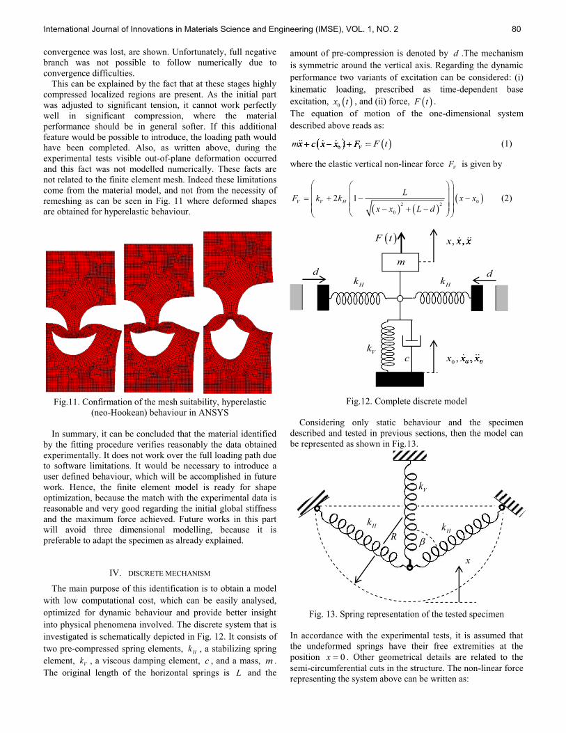
JOURNAL OF VOL. X, NO. X, MONTH X, 2014 6
convergence was lost, are shown. Unfortunately, full negative
branch was not possible to follow numerically due to
convergence difficulties.
This can be explained by the fact that at these stages highly
compressed localized regions are present. As the initial part
was adjusted to significant tension, it cannot work perfectly
well in significant compression, where the material
performance should be in general softer. If this additional
feature would be possible to introduce, the loading path would
have been completed. Also, as written above, during the
experimental tests visible out-of-plane deformation occurred
and this fact was not modelled numerically. These facts are
not related to the finite element mesh. Indeed these limitations
come from the material model, and not from the necessity of
remeshing as can be seen in Fig. 11 where deformed shapes
are obtained for hyperelastic behaviour.
Fig.11. Confirmation of the mesh suitability, hyperelastic
(neo-Hookean) behaviour in ANSYS
In summary, it can be concluded that the material identified
by the fitting procedure verifies reasonably the data obtained
experimentally. It does not work over the full loading path due
to software limitations. It would be necessary to introduce a
user defined behaviour, which will be accomplished in future
work. Hence, the finite element model is ready for shape
optimization, because the match with the experimental data is
reasonable and very good regarding the initial global stiffness
and the maximum force achieved. Future works in this part
will avoid three dimensional modelling, because it is
preferable to adapt the specimen as already explained.
IV. DISCRETE MECHANISM
The main purpose of this identification is to obtain a model
with low computational cost, which can be easily analysed,
optimized for dynamic behaviour and provide better insight
into physical phenomena involved. The discrete system that is
investigated is schematically depicted in Fig. 12. It consists of
two pre-compressed spring elements, Hk , a stabilizing spring
element, Vk , a viscous damping element, c , and a mass, m .
The original length of the horizontal springs is L and the
amount of pre-compression is denoted by d .The mechanism
is symmetric around the vertical axis. Regarding the dynamic
performance two variants of excitation can be considered: (i)
kinematic loading, prescribed as time-dependent base
excitation, 0
x t , and (ii) force, F t .
The equation of motion of the one-dimensional system
described above reads as:
0 Vmx c x x F F t (1)
where the elastic vertical non-linear force VF is given by
02 2
0
2 1V V H
LF k k x x
x x L d
(2)
Fig.12. Complete discrete model
Considering only static behaviour and the specimen
described and tested in previous sections, then the model can
be represented as shown in Fig.13.
Fig. 13. Spring representation of the tested specimen
In accordance with the experimental tests, it is assumed that
the undeformed springs have their free extremities at the
position 0x . Other geometrical details are related to the
semi-circumferential cuts in the structure. The non-linear force
representing the system above can be written as:
m
F t
Vk
Hk
Hk
0 0 0, ,x x x
, ,x x x
dd
c
Vk
HkH
k
x
R
International Journal of Innovations in Materials Science and Engineering (IMSE), VOL. 1, NO. 2 80
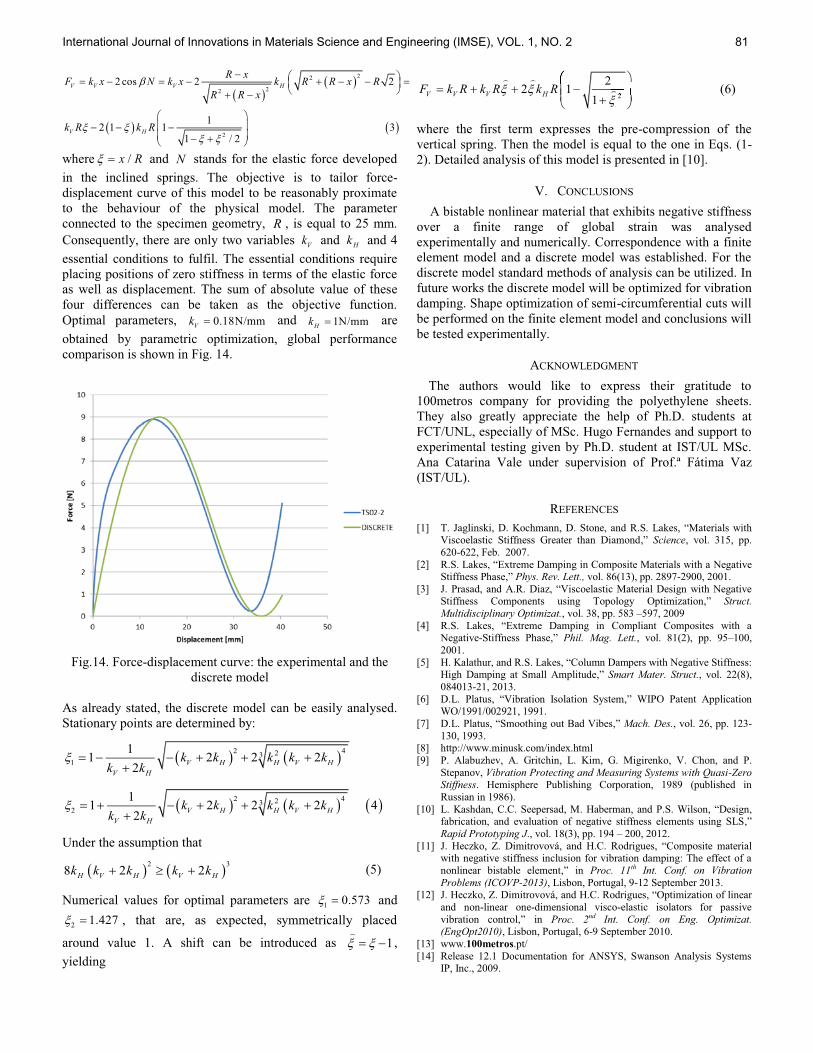
JOURNAL OF VOL. X, NO. X, MONTH X, 2014 7
22
22
2
2 cos 2 2
12 1 1 3
1 / 2
V V V H
V H
R xF k x N k x k R R x R
R R x
k R k R
where /x R and N stands for the elastic force developed
in the inclined springs. The objective is to tailor force-
displacement curve of this model to be reasonably proximate
to the behaviour of the physical model. The parameter
connected to the specimen geometry, R , is equal to 25 mm.
Consequently, there are only two variables Vk and H
k and 4
essential conditions to fulfil. The essential conditions require
placing positions of zero stiffness in terms of the elastic force
as well as displacement. The sum of absolute value of these
four differences can be taken as the objective function.
Optimal parameters, 0.18N/mmV
k and 1N/mmH
k are
obtained by parametric optimization, global performance
comparison is shown in Fig. 14.
Fig.14. Force-displacement curve: the experimental and the
discrete model
As already stated, the discrete model can be easily analysed.
Stationary points are determined by:
2 4231
11 2 2 2
2V H H V H
V H
k k k k kk k
2 4232
11 2 2 2 4
2V H H V H
V H
k k k k kk k
Under the assumption that
2 38 2 2
H V H V Hk k k k k (5)
Numerical values for optimal parameters are 10.573 and
21.427 , that are, as expected, symmetrically placed
around value 1. A shift can be introduced as 1,
yielding
2
22 1
1V V V H
F k R k R k R (6)
where the first term expresses the pre-compression of the
vertical spring. Then the model is equal to the one in Eqs. (1-
2). Detailed analysis of this model is presented in [10].
V. CONCLUSIONS
A bistable nonlinear material that exhibits negative stiffness
over a finite range of global strain was analysed
experimentally and numerically. Correspondence with a finite
element model and a discrete model was established. For the
discrete model standard methods of analysis can be utilized. In
future works the discrete model will be optimized for vibration
damping. Shape optimization of semi-circumferential cuts will
be performed on the finite element model and conclusions will
be tested experimentally.
ACKNOWLEDGMENT
The authors would like to express their gratitude to
100metros company for providing the polyethylene sheets.
They also greatly appreciate the help of Ph.D. students at
FCT/UNL, especially of MSc. Hugo Fernandes and support to
experimental testing given by Ph.D. student at IST/UL MSc.
Ana Catarina Vale under supervision of Prof.ª Fátima Vaz
(IST/UL).
REFERENCES
[1] T. Jaglinski, D. Kochmann, D. Stone, and R.S. Viscoelastic Stiffness Greater than Diamond Science, vol. 315, pp.
620-622, Feb. 2007.
[2] R.S. Negative Stiffness Phase Phys. Rev. Lett., vol. 86(13), pp. 2897-2900, 2001.
[3] J. Prasad, and A.R. Stiffness Components using Topology Optimization Struct.
Multidisciplinary Optimizat., vol. 38, pp. 583 597, 2009
[4] R.S. Negative-Stiffness Phase Phil. Mag. Lett., vol. 81(2), pp. 95 100,
2001.
[5] H. Kalathur, and R.S. High Damping at Small Amplitude Smart Mater. Struct., vol. 22(8),
084013-21, 2013.
[6] D.L. WIPO Patent Application WO/1991/002921, 1991.
[7] D.L. hing out Bad Vibes Mach. Des., vol. 26, pp. 123-
130, 1993. [8] http://www.minusk.com/index.html
[9] P. Alabuzhev, A. Gritchin, L. Kim, G. Migirenko, V. Chon, and P.
Stepanov, Vibration Protecting and Measuring Systems with Quasi-Zero Stiffness. Hemisphere Publishing Corporation, 1989 (published in
Russian in 1986).
[10] L. Kashdan, C.C. Seepersad, M. Haberman, and P.S. fabrication, and evaluation of negative stiffness elements using SLS
Rapid Prototyping J., vol. 18(3), pp. 194 200, 2012.
[11] J. Heczko, Z. Dimitrovová, and H.C. with negative stiffness inclusion for vibration damping: The effect of a
nonlinear bistable element in Proc. 11th Int. Conf. on Vibration
Problems (ICOVP-2013), Lisbon, Portugal, 9-12 September 2013. [12] J. Heczko, Z. Dimitrovová, and H.C.
and non-linear one-dimensional visco-elastic isolators for passive
vibration control in Proc. 2nd Int. Conf. on Eng. Optimizat. (EngOpt2010), Lisbon, Portugal, 6-9 September 2010.
[13] www.100metros
[14] Release 12.1 Documentation for ANSYS, Swanson Analysis Systems IP, Inc., 2009.
International Journal of Innovations in Materials Science and Engineering (IMSE), VOL. 1, NO. 2 81
Design Criteria for a Pendulum Absorber to Control High Building
Vibrations
F. S. Oliveira1, A. L. Z. Gomez
1, S. M. Avila *
2, and J. L. V. Brito
1
1Civil and Environmental Engineering Department, University of Brasilia, Brazil
2Gama Engineering College, University of Brasilia, Brazil
Abstract The increasing development of structural analysis
techniques, the appearance of more resistant materials, and the
high cost of construction in big metropolis, caused an elevation
on the height of buildings, making these structures considerably
more vulnerable to actions of dynamic loads such as wind and
earthquakes. Due to the problems caused by the action of these
dynamic loads, vibration control has become a relevant issue in
Civil Engineering. One of the most used vibration control systems
is the Tuned Mass Damper (TMD). It basically consist of a mass-
spring-damper system attached to the main structure, the
frequency of the damper is tuned to a particular frequency, with
the goal of making the TMD vibrate out of phase with the main
system, thus transferring the energy system to the damper. The
present study purpose is to evaluate the efficiency of a pendulum
TMD when the structure is subjected to dynamic loads such as
random excitation, given by power spectral density functions,
and harmonic loads. Analytical expressions are derived,
minimizing the mean square value of the power spectral
density.Also parametric studies are performed to define design
criteria, performingfrequency response function minimization,
searching its minimum maximum amplitudes iteratively. The
behavior of a ten storey shear building is analyzed, reducing it to
one degree of freedom through modal analysis. A pendulum
TMD is attached to it, considering the optimal parameters
obtained in this work. A set of general dimensionless optimal
parameters for a pendulum TMD are presented in this study,
they can be employed to the design of a pendulum to control any
tall building, subjected to random dynamic loads, with different
mass and damping ratios.
Keywords Passive Control, Structural Control, Structural
Dynamics, Tuned Mass Damper
I. INTRODUCTION
The increasing development of structural analysis
techniques, the appearance of more resistant materials, and the
high cost of construction in big metropolis, caused an
elevation on the height of buildings, making these structures
considerably more vulnerable to actions of dynamic loads
such as wind and earthquakes. This kind of vibrations is
undesirable, not only because of structural safety but also
human comfort [1].
Thus concern about civil structures protection including its
contents and occupants is a global reality. An alternative
,widely studied in the last years, is the structural control.
Originally developed in aerospace engineering, this
technology was extended for civil engineering problems to
protect bridges and high buildings from excessive dynamic
loads. Structural control fundamentally changes structure
stiffness and damping properties, adding external device or
applying external forces. It is classified on passive, active,
hybrid or semi-active control [1-2].
Widely studied in the last years, passive control consists in
adding one or more devices to the structure to absorb or
transfer part of the energy from to the main structure. Passive
control typical mechanisms are: mass dampers that control
structural response by transferring the energy between the
main structure and an auxiliary mass; structural dampers that
dissipate energy while deforming themselves and base
isolation systems that uncouple structure moving from seismic
soil vibrations.
A tuned mass damper (TMD) is a device composed by a
mass-spring-dashpot attached to the structure aiming to reduce
structural vibration response [2]. The beginning of TMD
appliance to civil structures was at the sixties on high
buildings, bridges, towers and industrial chimneys to control
vibrations caused by wind forces. A TMD tuned to the first
structure natural frequency reduces substantially the response
associated to the first mode vibration while little reducing or
even increasing the response associated to higher modes.
Moreover, a single TMD is more sensitive to discrepancies on
the first natural frequency and/or damping ratio considered on
the design. These limitations can be overcome by adding more
than one damper, each one of them tuned to a different
vibration natural frequency [3].
One of the alternative geometries of the TMD is the
pendulum shape [4]. The pendulum is attached to the structure
and its movement excites the device transferring portion of the
energy from one system to another, reducing this way
structural member request of energy dissipation. This type of
damper has its vibration period depending on the length of the
cable, and can only be considered a linear device when the
vibration amplitudes are small.
Lourenço [5] described the design, construction,
implementation and performance of a prototype adaptative
pendulum tuned mass damper (APTMD), demonstrating the
performance improvements obtained when the tuned mass
damper (TMD) parameters are optimized. In his study was
considered the effect of adjusting the APTMD tuned
frequency and damping ratio on a two storey test structure
subjected to broadband and narrowband excitation.
Orlando and Goncalves [6] evaluated a pendulum TMD to
control excessive vibrations in slender towers, it is presented a
parametric analysis of non-linear oscillations of a tower-
damper system searching the best configurations to reduce
vibrations and tower construction.
Gerges and Vickery [7] studied the behavior of a pendulum
TMD to reduce the structure rms displacement subjected to
force and accelerations simulating random excitations such as
white noise. A numerical studied was performed to obtain
© 2014 EDUGAIT Press
International Journal of Innovations in Materials Science and Engineering (IMSE), VOL. 1, NO. 2 82

optimal parameters to a damped main system subjected to
seismic and wind loads.
Morga and Marano [8] investigate two different
optimization criteria of TMDs applied to a slender structure
excited by wind load: the reduction of the maximum
displacement at the top of the structure; the reduction of the
maximum inertial acceleration at the top of the structure. The
wind load is defined by a superposition of the mean wind
velocity and a filtered white noise.
The present study purpose is to evaluate the efficiency of a
pendulum TMD when the structure is subjected to dynamic
loads such as random excitation, given by power spectral
density functions, and deterministic harmonic loads.
The behavior of a high building is analyzed, reducing it to
one degree of freedom through modal analysis [2]. Two load
cases are studied, the structure subject to a dynamic force and
to a base acceleration. A pendulum TMD is attached to it in
order to reduce excessive dynamic response.
Optimum parameters for the undamped case are obtained
analytically minimizing the mean square value of the
dimensionless displacement, considering an excitation of a
white noise random force. Considering damping effects it is
no longer possible to obtain an analytical solution, so in these
cases parametric studies were performed. This numerical
procedure is based on the MinMax method [9]. The design
criteria are obtained through frequency response function
minimization searching its minimum maximum amplitudes.
This minimization is achieved by an optimization iterative
process.
A set of general dimensionless optimal parameters for a
pendulum TMD are presented in this research, they can be
employed to the design of a pendulum to control any tall
building, subjected to deterministic or random dynamic loads,
with different mass and damping ratios.
II. MATHEMATICAL FORMULATION
1) Response frequency function to a system excited by
harmonic force and base acceleration
Fig. 1 shows a schematic description of a pendulum TMD
attached to a main system composing a two degree of freedom
model DOF, the main system is reduced to a 1 DOF model
corresponding to the mode to be controlled [2]. Fig. 1 presents
the main system subjected to a force Fs(t) and Fig.2 the
system subjected to a base acceleration .
The equation of motion considering small displacement to
Fig. 1 system are:
(1)
(2)
and to Figure 2 system are:
(3)
(4)
Where main system modal mass; main system
modal damping; main system modal stiffness;
pendulum mass; pendulum damping; pendulum
stiffness; cable length; gravity acceleration;
excitation modal force; main system displacement;
pendulum angular displacement; relative displacement
of the main system to the base ;
main system absolute displacement; base displacement;
base acceleration. The pendulum natural frequency is
.
(
t
)
Mp
L
Ms
Ks
Cs
Fs(t)
y(t)
Fig. 1 Structure with a linear pendulum attached: excitation due to a force Fs(t)
(
t
)
Mp
L
Ms
Ks
Cs
y (t)
y (t)
1
0
Fig. 2 Structure with a linear pendulum attached: excitation due to a base
acceleration
These equations can be rewritten using the following
dimensionless terms:
(5)
(6)
(7)
Substituting Eqs.(5-7) into Eqs. (1-4) the following
equations are obtained:
International Journal of Innovations in Materials Science and Engineering (IMSE), VOL. 1, NO. 2 83
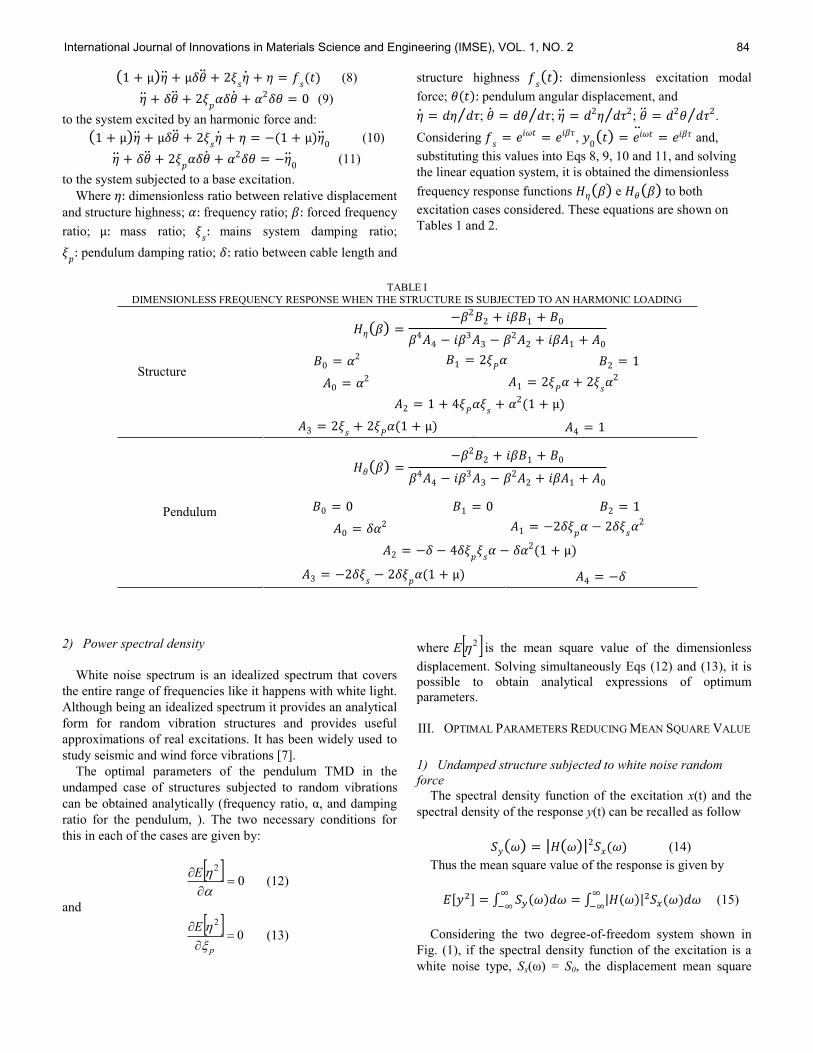
(8)
(9)
to the system excited by an harmonic force and:
(10)
(11)
to the system subjected to a base excitation.
Where dimensionless ratio between relative displacement
and structure highness; frequency ratio; forced frequency
ratio; mass ratio; mains system damping ratio;
pendulum damping ratio; ratio between cable length and
structure highness dimensionless excitation modal
force; pendulum angular displacement, and
; ; ; .
Considering , and,
substituting this values into Eqs 8, 9, 10 and 11, and solving
the linear equation system, it is obtained the dimensionless
frequency response functions e to both
excitation cases considered. These equations are shown on
Tables 1 and 2.
TABLE I
DIMENSIONLESS FREQUENCY RESPONSE WHEN THE STRUCTURE IS SUBJECTED TO AN HARMONIC LOADING
Structure
Pendulum
2) Power spectral density
White noise spectrum is an idealized spectrum that covers
the entire range of frequencies like it happens with white light.
Although being an idealized spectrum it provides an analytical
form for random vibration structures and provides useful
approximations of real excitations. It has been widely used to
study seismic and wind force vibrations [7].
The optimal parameters of the pendulum TMD in the
undamped case of structures subjected to random vibrations
ratio for the pendulum, ). The two necessary conditions for
this in each of the cases are given by:
02E
(12)
and
02
p
E (13)
where 2E is the mean square value of the dimensionless
displacement. Solving simultaneously Eqs (12) and (13), it is
possible to obtain analytical expressions of optimum
parameters.
III. OPTIMAL PARAMETERS REDUCING MEAN SQUARE VALUE
1) Undamped structure subjected to white noise random
force
The spectral density function of the excitation x(t) and the
spectral density of the response y(t) can be recalled as follow
(14)
Thus the mean square value of the response is given by
(15)
Considering the two degree-of-freedom system shown in
Fig. (1), if the spectral density function of the excitation is a
white noise type, Sx S0, the displacement mean square
International Journal of Innovations in Materials Science and Engineering (IMSE), VOL. 1, NO. 2 84

value is given by
(16)
Considering the equation of H , given by Table 1, the
integral of Eq. (16) are carried out according to the table given
by [10].
TABLE II DIMENSIONLESS FREQUENCY RESPONSE WHEN THE STRUCTURE IS SUBJECTED TO AN HARMONIC BASE ACCELERATION
Structure
Pendulum
Solving simultaneously Eqs. (12) and (13) and performing
algebraic manipulations the following expressions are
obtained
(17)
(18)
3) Undamped structure subjected to white noise random base
acceleration
Analogously to the previous case for a two degree-of-
system, shown in Fig. (2) subjected to a random base
acceleration with white noise spectral density function,
Sx = S0, the displacement mean square value is given by
Eq. (16).
Performing the same optimization described to the white
noise random force the following optimum expressions are
obtained
(19)
(20)
IV. NUMERICAL STUDY
When taking damping effect into account, it is no longer
possible to obtain the analytical solution for the optimum
parameters of the pendulum, so in these cases it is necessary to
use a numerical search procedure.
This work used MinMax numerical procedure to minimize
the maximum amplitude of the frequency response when the
structure is subjected to an harmonic force.
Tsai and Lin [9] showed for undamped system cases that
the reduction of resonance peak to its lowest value occurs
using Den Hartog [11] values, as well as, through MinMax
numerical search in which are performed various parameter
combinations in order to store those representing the lowest
maximum amplitude.
Therefore, repeated tries are performed varying each one of
the parameters in the frequency response function, in every try
the parameter range to be analyzed is fixed as well as the
International Journal of Innovations in Materials Science and Engineering (IMSE), VOL. 1, NO. 2 85

discretization of this range. When the numerical search is
completed, a new range with values near of those that improve
the TMD performance is considered to perform a new try.
The computational routine varies the system parameters
(mass ratio, pendulum damping ratio, main structure damping
ratio, frequency ratio, forced frequency ratio) and calculates
the frequency response function value for each one of the
analyzed cases. After it is stored the less response value found
in all parameter combinations. The numerical search is ended
when all parameters are combined, and the combination that
produced the lowest response provides the optimal parameters.
Fig. 3 compares the frequency response obtained to an
undamped case using Den Hartog [11] parameters, the
MinMax parameters and considering the uncontrolled case. It
can be observed a similar behavior between the two controlled
cases.
Vibration amplitudes for damped systems with
don´t have the same behavior of the undamped systems.
Frequency response curves to different damping ratios don´t
have fixed points, therefore closed solution for optimal
parameters cannot be determined in the same way of the
undamped case. However, optimal parameters can be found
through a numerical search in a way to minimize the response
peak.
Fig.3 Dimensionless frequency response of the structure subjected to an harmonic force with Den Hartog and MinMax parameters
To determine optimal values to , e to specific values
of e , it is performed a numerical iterative procedure
where various values of e are combined on the response
function equation in a way to define maximum amplitudes
values. Once found and stored the maximum amplitudes, a
new search is performed to find the lowest of them, in other
words, the parameters that define the minimum maximal
amplitudes are found. It is noteworthy that parameters
presented on Tables 3 and 4 are general and therefore valid to
any structure.
Figs. 4 and 5 compare optimal values of damping ratio ( ),
obtained varying mass ratio and considering . It is
noticed good agreement between the two analyses.
Fig. 4 Optimaldampingratiocomparison.
TABLE III
OPTIMAL PENDULUM PARAMETERS FOR A STRUCTURE SUBMITTED TO AN HARMONIC FORCE
-4.00
1.00
6.00
11.00
16.00
0.70 0.80 0.90 1.00 1.10 1.20 1.30
H(
)
Min Max Den Hartog Uncontrolled
0.040
0.065
0.090
0.115
0.140
0.165
0.190
0.000 0.025 0.050 0.075 0.100
p
µ
Minmax Tsai & Lin
International Journal of Innovations in Materials Science and Engineering (IMSE), VOL. 1, NO. 2 86
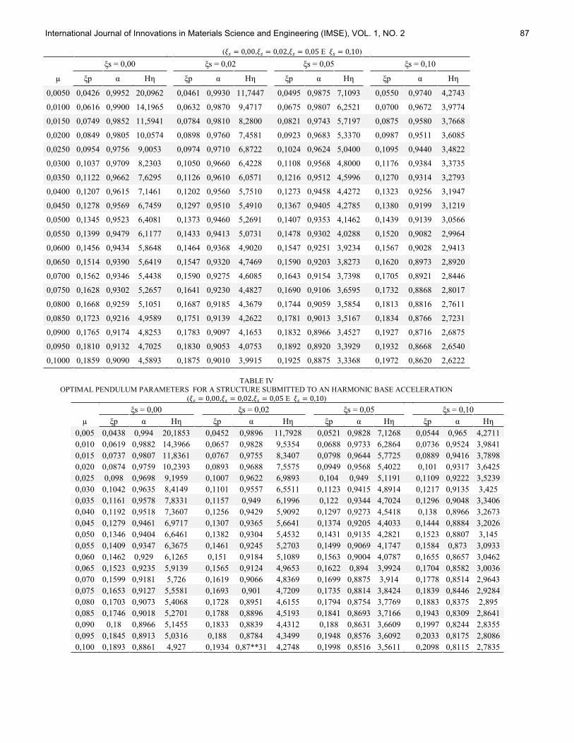
( , , E )
µ
0,0050 0,0426 0,9952 20,0962 0,0461 0,9930 11,7447 0,0495 0,9875 7,1093 0,0550 0,9740 4,2743
0,0100 0,0616 0,9900 14,1965 0,0632 0,9870 9,4717 0,0675 0,9807 6,2521 0,0700 0,9672 3,9774
0,0150 0,0749 0,9852 11,5941 0,0784 0,9810 8,2800 0,0821 0,9743 5,7197 0,0875 0,9580 3,7668
0,0200 0,0849 0,9805 10,0574 0,0898 0,9760 7,4581 0,0923 0,9683 5,3370 0,0987 0,9511 3,6085
0,0250 0,0954 0,9756 9,0053 0,0974 0,9710 6,8722 0,1024 0,9624 5,0400 0,1095 0,9440 3,4822
0,0300 0,1037 0,9709 8,2303 0,1050 0,9660 6,4228 0,1108 0,9568 4,8000 0,1176 0,9384 3,3735
0,0350 0,1122 0,9662 7,6295 0,1126 0,9610 6,0571 0,1216 0,9512 4,5996 0,1270 0,9314 3,2793
0,0400 0,1207 0,9615 7,1461 0,1202 0,9560 5,7510 0,1273 0,9458 4,4272 0,1323 0,9256 3,1947
0,0450 0,1278 0,9569 6,7459 0,1297 0,9510 5,4910 0,1367 0,9405 4,2785 0,1380 0,9199 3,1219
0,0500 0,1345 0,9523 6,4081 0,1373 0,9460 5,2691 0,1407 0,9353 4,1462 0,1439 0,9139 3,0566
0,0550 0,1399 0,9479 6,1177 0,1433 0,9413 5,0731 0,1478 0,9302 4,0288 0,1520 0,9082 2,9964
0,0600 0,1456 0,9434 5,8648 0,1464 0,9368 4,9020 0,1547 0,9251 3,9234 0,1567 0,9028 2,9413
0,0650 0,1514 0,9390 5,6419 0,1547 0,9320 4,7469 0,1590 0,9203 3,8273 0,1620 0,8973 2,8920
0,0700 0,1562 0,9346 5,4438 0,1590 0,9275 4,6085 0,1643 0,9154 3,7398 0,1705 0,8921 2,8446
0,0750 0,1628 0,9302 5,2657 0,1641 0,9230 4,4827 0,1690 0,9106 3,6595 0,1732 0,8868 2,8017
0,0800 0,1668 0,9259 5,1051 0,1687 0,9185 4,3679 0,1744 0,9059 3,5854 0,1813 0,8816 2,7611
0,0850 0,1723 0,9216 4,9589 0,1751 0,9139 4,2622 0,1781 0,9013 3,5167 0,1834 0,8766 2,7231
0,0900 0,1765 0,9174 4,8253 0,1783 0,9097 4,1653 0,1832 0,8966 3,4527 0,1927 0,8716 2,6875
0,0950 0,1810 0,9132 4,7025 0,1830 0,9053 4,0753 0,1892 0,8920 3,3929 0,1932 0,8668 2,6540
0,1000 0,1859 0,9090 4,5893 0,1875 0,9010 3,9915 0,1925 0,8875 3,3368 0,1972 0,8620 2,6222
TABLE IV
OPTIMAL PENDULUM PARAMETERS FOR A STRUCTURE SUBMITTED TO AN HARMONIC BASE ACCELERATION
( , , E )
µ
0,005 0,0438 0,994 20,1853 0,0452 0,9896 11,7928 0,0521 0,9828 7,1268 0,0544 0,965 4,2711
0,010 0,0619 0,9882 14,3966 0,0657 0,9828 9,5354 0,0688 0,9733 6,2864 0,0736 0,9524 3,9841
0,015 0,0737 0,9807 11,8361 0,0767 0,9755 8,3407 0,0798 0,9644 5,7725 0,0889 0,9416 3,7898
0,020 0,0874 0,9759 10,2393 0,0893 0,9688 7,5575 0,0949 0,9568 5,4022 0,101 0,9317 3,6425
0,025 0,098 0,9698 9,1959 0,1007 0,9622 6,9893 0,104 0,949 5,1191 0,1109 0,9222 3,5239
0,030 0,1042 0,9635 8,4149 0,1101 0,9557 6,5511 0,1123 0,9415 4,8914 0,1217 0,9135 3,425
0,035 0,1161 0,9578 7,8331 0,1157 0,949 6,1996 0,122 0,9344 4,7024 0,1296 0,9048 3,3406
0,040 0,1192 0,9518 7,3607 0,1256 0,9429 5,9092 0,1297 0,9273 4,5418 0,138 0,8966 3,2673
0,045 0,1279 0,9461 6,9717 0,1307 0,9365 5,6641 0,1374 0,9205 4,4033 0,1444 0,8884 3,2026
0,050 0,1346 0,9404 6,6461 0,1382 0,9304 5,4532 0,1431 0,9135 4,2821 0,1523 0,8807 3,145
0,055 0,1409 0,9347 6,3675 0,1461 0,9245 5,2703 0,1499 0,9069 4,1747 0,1584 0,873 3,0933
0,060 0,1462 0,929 6,1265 0,151 0,9184 5,1089 0,1563 0,9004 4,0787 0,1655 0,8657 3,0462
0,065 0,1523 0,9235 5,9139 0,1565 0,9124 4,9653 0,1622 0,894 3,9924 0,1704 0,8582 3,0036
0,070 0,1599 0,9181 5,726 0,1619 0,9066 4,8369 0,1699 0,8875 3,914 0,1778 0,8514 2,9643
0,075 0,1653 0,9127 5,5581 0,1693 0,901 4,7209 0,1735 0,8814 3,8424 0,1839 0,8446 2,9284
0,080 0,1703 0,9073 5,4068 0,1728 0,8951 4,6155 0,1794 0,8754 3,7769 0,1883 0,8375 2,895
0,085 0,1746 0,9018 5,2701 0,1788 0,8896 4,5193 0,1841 0,8693 3,7166 0,1943 0,8309 2,8641
0,090 0,18 0,8966 5,1455 0,1833 0,8839 4,4312 0,188 0,8631 3,6609 0,1997 0,8244 2,8355
0,095 0,1845 0,8913 5,0316 0,188 0,8784 4,3499 0,1948 0,8576 3,6092 0,2033 0,8175 2,8086
0,100 0,1893 0,8861 4,927 0,1934 0,87**31 4,2748 0,1998 0,8516 3,5611 0,2098 0,8115 2,7835
International Journal of Innovations in Materials Science and Engineering (IMSE), VOL. 1, NO. 2 87

Fig. 5 Optimalmassratiocomparison
Figs.6 to 9shows a comparison between optimal parameters
obtained via numerical search and those obtained analytically
S = 0, considering the two
excitation cases: force and base acceleration.
Fig 6 Optimal frequency ratio (force)
Fig 7 optimal damping ratio (force)
Fig.8 Optimal frequency ratio (base acceleration)
Fig9 Optimal damping ratio (base acceleration)
In a way to verify the pendulum TMD effectiveness using
the optimized design criteria, the main structure is subjected to
a Kanai-Tajimi spectrum representing random seismic base
acceleration.
The power spectral density function of Kanai Tajimi can be
interpreted as an ideal white noise excitation filtered by
underground soil extracts on site, which is given by
(21)
whereS0 is the white noise spectrum, f the frequency, and
and fg are the ground damping and frequency respectively. The
values assigned in numerical simulations in this work
are: =0.6 and fg= 2.39 Hz (15 rad/s).
Fig. 9 shows the dimensionless displacement time-history
without control and controlled by the two proposed design
criteria, considering the structure subjected to records
resulting from Kanai-Tajimi spectrum. It can be observed that
0.900
0.920
0.940
0.960
0.980
1.000
0.000 0.020 0.040 0.060 0.080 0.100µ
Minmax Tsai & Lin
0.9000
0.9200
0.9400
0.9600
0.9800
1.0000
0.000 0.020 0.040 0.060 0.080 0.100
µMinMax Min. Spectral Density
0.0000
0.0200
0.0400
0.0600
0.0800
0.1000
0.1200
0.1400
0.1600
0.1800
0.2000
0.000 0.020 0.040 0.060 0.080 0.100
p
µ
MinMax Min. Spectral Density
0.8000
0.8200
0.8400
0.8600
0.8800
0.9000
0.9200
0.9400
0.9600
0.9800
1.0000
0.000 0.020 0.040 0.060 0.080 0.100
µMinMax Min. Spectral Density
0.0000
0.0200
0.0400
0.0600
0.0800
0.1000
0.1200
0.1400
0.1600
0.1800
0.2000
0.000 0.020 0.040 0.060 0.080 0.100
p
µMinMax Min. Spectral Density
International Journal of Innovations in Materials Science and Engineering (IMSE), VOL. 1, NO. 2 88

the two design criteria lead to very similar response reducing
it most of the time analyzed.
Fig. 10 Dimensionless displacement time-history (Kanai-Tajimi)
V. CONCLUSIONS
The TMD optimization aiming to reduce response function
amplitude to an undamped structure subjected to an harmonic
force was originally performed by Den Hartog [11]. However,
all types of structural systems have some level of damping,
moreover civil structures are subjected to random loads such
as wind forces and earthquakes. An alternative geometry to
the auxiliary system of the TMD is a pendulum, which fits
very well to be installed in high buildings in practice. This
work proposes design criteria to TMD pendulum types
installed on high buildings subjected to different types of
deterministic and random loadings. Performing minimization
procedures a set of optimal parameters depending on the mass
and damping of the main structure are proposed. It is
noteworthy that parameters presented are valid to any tall
building. It was verified that Minmax procedure is an efficient
tool to pendulum TMD optimization. Using the suggested
parameters in this work will improve considerably pendulum
performance on reducing amplitude vibrations.
VI. REFERENCES
[1] S. M. Avila, Hybrid control for vibration attenuation in
buildings PhD thesis, CatholicUniversityof Rio de Janeiro, Rio de
Janeiro, BrasilZ, 2002. (In Portuguese) [2] T. T. Soong, T. T and G. F. Dargush,.Passive Energy Dissipation
Systems in Structural Engineering. Chichester: John Wiley & Sons,
1997. [3] R. B. Carneiro; S. M. Avila and J. L. V. Brito, Parametric study on
multiple tuned mass dampers using interconnected
masses .International Journal of Structural Stability and Dynamics, vol. 8, pp. 187-202, 2008.
[4] F. S. Oliveira,. Design Criteria for Pendulum Type Absorber for
Vibration Control in Tall Buildings . Master's Dissertation Dep. of Civil Eng, University of Brasilia, 2012. (In Portuguese)
[5] R. Lourenco, Design, Construction and Testing of an Adaptive Pendulum Tuned Mass Damper Master - Waterloo,
Ontario, Canada, 2011.
[6] D. OrlandoandP. B. Goncalves, Hybrid nonlinear control of a tall tower with a pendulum absorber Structural Engineering and
Mechanics, vol. 46, pp. 153-177, 2013.
[7] R. R. GergesandB. J. Vickery, Optimum design of pendulum-type tuned mass dampers. The Structural Design of Tall and Special
Buildings.vol. 14(4), pp. 353-368, 2005.
[8] M. Morga, and G. C. Marano, Optimization criteria of TMD to reduce vibrations generated by the wind in a slender
structure Journal of Vibration and Control, v.0(0), pp. 1-13, 2013
(published online). [9] Optimum tuned-mass dampers for
minimizing steady-state response of support-excited and damped
22(11), pp. 957-973, 1993.
[10] Crandall S. H. and Mark M. D., Random Vibration in Mechanical
Analysis, Academic Press, 1963 [11] J. P. Den Hartog, Mechanical vibrations. McGraw-Hill, New York,
1956.
-1.00E-03
-5.00E-04
0.00E+00
5.00E-04
1.00E-03
0 10 20 30 40 50 60 70 80 90 100 110 120 130
Dim
en
sio
nle
ss d
isp
lace
me
nt
())
Time( ))
MinMax Min. Spectral Density Uncontrolled
International Journal of Innovations in Materials Science and Engineering (IMSE), VOL. 1, NO. 2 89

Seismic Performance of a Tall Diagrid Steel Building with Tuned Mass
Dampers
Andre R. Barbosa*1, and Garlan Ramadhan**
2
1Assistant Professor, School of Civil and Construction Engineering, Oregon State University, Corvallis, OR 97331, USA2Graduate Student, School of Civil and Construction Engineering, Oregon State University, Corvallis, OR 97331, USA
*[email protected], **[email protected]
Abstract⎯ The steel diagrid structural system is a recent load
bearing and lateral resisting structural system for tall building
structures that is relatively unexplored in the western United
States. One possible reason for the little use of diagrid systems in
earthquake prone regions is the lack of guidelines and
application examples illustrating the design and analysis of these
structures. In this work, a 72-story prototype building is used as
an example for which the design and analysis of the diagrid
system is performed. To mitigate the possible large displacement
and base shear demands that these structures may undergo
under seismic events, two new design solutions consisting of one
or two friction tuned mass damper (TMD) units are explored. In
the first solution, a TMD is placed on the top four stories of the
building and is tuned to reduce the contribution of the
fundamental mode of vibration of the structure, in both
horizontal directions. In the second solution, a double TMD
system is added at mid-height of the building, in which a second
TMD unit in tuned to the second period of the structure.. Using a
nonlinear finite element model of the tuned mass damper, the
effectiveness of the friction mass damper design is studied. The
mass damper system consists of a concrete tank containing sand
or water. The tank is placed in between the building reinforced
concrete structural core and the exterior steel diagrid system.
This mass damper is connected to the structure using friction
pendulum isolators that are chosen due to their ability to
undergo large deformations. The models are then subjected to
accelerograms from historical shallow crustal earthquakes and
subduction zone earthquakes. Parametric studies are carried out
to understand the influence of different parameters of the mass
damper design in improving the seismic performance of the
building. Improvement of the seismic performance is assessed in
terms of minimization of inter-story drift ratios, base shear
forces, as well as floor absolute accelerations. The results show
that the single TMD system can reduce significantly the peak
base reaction and inter-story drift envelopes. Addition of the
second TMD provides further improvements in terms of reducing
the peak base reactions, while also producing notable reductions
in peak absolute floor accelerations, which are not observed when
only one TMD unit is used.
Keywords— Cascadia Subduction Zone Earthquakes, Diagrid,
Earthquakes, Friction Pendulum Isolator, Nonlinear Structural
Analysis, Seismic Design, Steel Structures, Tall Buildings, Tuned
Mass Damper.
I. INTRODUCTION
HE FIRST tall buildings were built in United States of
America in the late nineteenth century [1]. There is no set
definition for what constitutes a tall building, but often
buildings that are 14 stories or more are considered as tall
buildings (50 m or taller). At present times, many tall
buildings have been built around the world and The Council
on Tall Buildings and Urban Habitat contains information on
more than ten thousand tall buildings [2]. Several structural
systems have also been developed to realize mankind’s dream
in pursuing new heights and allow for the design of tall
buildings. Out of many structural systems, the outer steel
diagrid structural system with reinforced concrete inner core is
but one of them. The diagrid structural system gets its name
from the diagonal columns that form triangular trusses.
Diagrid is an abbreviation for “diagonal grid” of trusses. The
diagonal trusses are connected by horizontal rings (steel
beams), which provide support for the floors and column
buckling restrains. The diagonal members carry gravity loads
as well as lateral loads, and thus steel is typically used in
diagrid structures. The main difference between conventional
steel exterior-braced frame trusses (X, K, V, and Chevron type
braces) is that in the diagrid structural system almost all
vertical columns are typically eliminated. The interior
reinforced concrete core typically consists of walls and is
designed not only to resist lateral loading, but also to allow for
the vertical communication and transport of people (elevator
shafts and stairwells), heating, ventilation, and air
conditioning, plumbing, electrical, and fire protection systems.
The diagrid structural system is known for its redundancy,
continuous and uninterrupted load paths, and is thus
considered to be a very efficient structural system [3].
However, these efficiencies also come with drawbacks. Most
new structures that have been designed and built using this
system are lighter and more flexible than conventional tall
building systems, and thus can suffer large displacements,
especially under wind and seismic loading. Some prime
examples of this kind of structures are the Hearst Tower, in
New York City, the China Central Television (CCTV)
Headquarters in Beijing, China, and the Tornado Tower in
Doha, Qatar.
The diagrid structural system is relatively new and
unexplored in the Western United States and other high-
seismic regions of the world, and hence engineers lack the
guidelines and examples that can be used to promote the
design of tall buildings using such a structural system. This
paper addresses this gap in the literature, as the main objective
of this paper is to provide an example in the design and
analysis of diagrid structural systems for seismic regions, by
T
© 2014 EDUGAIT Press
International Journal of Innovations in Materials Science and Engineering (IMSE), VOL. 1, NO. 2 90
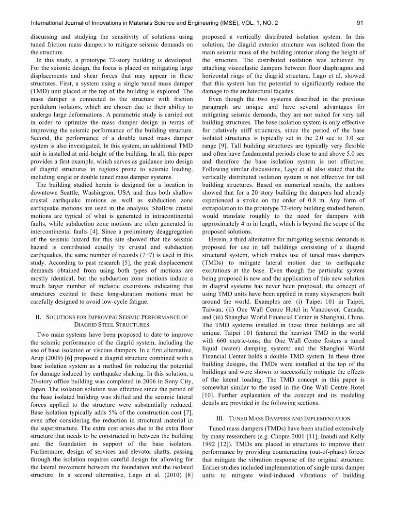
discussing and studying the sensitivity of solutions using
tuned friction mass dampers to mitigate seismic demands on
the structure.
In this study, a prototype 72-story building is developed.
For the seismic design, the focus is placed on mitigating large
displacements and shear forces that may appear in these
structures. First, a system using a single tuned mass damper
(TMD) unit placed at the top of the building is explored. The
mass damper is connected to the structure with friction
pendulum isolators, which are chosen due to their ability to
undergo large deformations. A parametric study is carried out
in order to optimize the mass damper design in terms of
improving the seismic performance of the building structure.
Second, the performance of a double tuned mass damper
system is also investigated. In this system, an additional TMD
unit is installed at mid-height of the building. In all, this paper
provides a first example, which serves as guidance into design
of diagrid structures in regions prone to seismic loading,
including single or double tuned mass damper systems.
The building studied herein is designed for a location in
downtown Seattle, Washington, USA and thus both shallow
crustal earthquake motions as well as subduction zone
earthquake motions are used in the analysis. Shallow crustal
motions are typical of what is generated in intracontinental
faults, while subduction zone motions are often generated in
intercontinental faults [4]. Since a preliminary deaggregation
of the seismic hazard for this site showed that the seismic
hazard is contributed equally by crustal and subduction
earthquakes, the same number of records (7+7) is used in this
study. According to past research [5], the peak displacement
demands obtained from using both types of motions are
mostly identical, but the subduction zone motions induce a
much larger number of inelastic excursions indicating that
structures excited to these long-duration motions must be
carefully designed to avoid low-cycle fatigue.
II. SOLUTIONS FOR IMPROVING SEISMIC PERFORMANCE OF
DIAGRID STEEL STRUCTURES
Two main systems have been proposed to date to improve
the seismic performance of the diagrid system, including the
use of base isolation or viscous dampers. In a first alternative,
Arup (2009) [6] proposed a diagrid structure combined with a
base isolation system as a method for reducing the potential
for damage induced by earthquake shaking. In this solution, a
20-story office building was completed in 2006 in Sony City,
Japan. The isolation solution was effective since the period of
the base isolated building was shifted and the seismic lateral
forces applied to the structure were substantially reduced.
Base isolation typically adds 5% of the construction cost [7],
even after considering the reduction in structural material in
the superstructure. The extra cost arises due to the extra floor
structure that needs to be constructed in between the building
and the foundation in support of the base isolators.
Furthermore, design of services and elevator shafts, passing
through the isolation requires careful design for allowing for
the lateral movement between the foundation and the isolated
structure. In a second alternative, Lago et al. (2010) [8]
proposed a vertically distributed isolation system. In this
solution, the diagrid exterior structure was isolated from the
main seismic mass of the building interior along the height of
the structure. The distributed isolation was achieved by
attaching viscoelastic dampers between floor diaphragms and
horizontal rings of the diagrid structure. Lago et al. showed
that this system has the potential to significantly reduce the
damage to the architectural façades.
Even though the two systems described in the previous
paragraph are unique and have several advantages for
mitigating seismic demands, they are not suited for very tall
building structures. The base isolation system is only effective
for relatively stiff structures, since the period of the base
isolated structures is typically set in the 2.0 sec to 3.0 sec
range [9]. Tall building structures are typically very flexible
and often have fundamental periods close to and above 5.0 sec
and therefore the base isolation system is not effective.
Following similar discussions, Lago et al. also stated that the
vertically distributed isolation system is not effective for tall
building structures. Based on numerical results, the authors
showed that for a 20 story building the dampers had already
experienced a stroke on the order of 0.8 m. Any form of
extrapolation to the prototype 72-story building studied herein,
would translate roughly to the need for dampers with
approximately 4 m in length, which is beyond the scope of the
proposed solutions.
Herein, a third alternative for mitigating seismic demands is
proposed for use in tall buildings consisting of a diagrid
structural system, which makes use of tuned mass dampers
(TMDs) to mitigate lateral motion due to earthquake
excitations at the base. Even though the particular system
being proposed is new and the application of this new solution
in diagrid systems has never been proposed, the concept of
using TMD units have been applied in many skyscrapers built
around the world. Examples are: (i) Taipei 101 in Taipei,
Taiwan; (ii) One Wall Centre Hotel in Vancouver, Canada;
and (iii) Shanghai World Financial Center in Shanghai, China.
The TMD systems installed in these three buildings are all
unique. Taipei 101 featured the heaviest TMD in the world
with 660 metric-tons; the One Wall Centre fosters a tuned
liquid (water) damping system; and the Shanghai World
Financial Center holds a double TMD system. In these three
building designs, the TMDs were installed at the top of the
buildings and were shown to successfully mitigate the effects
of the lateral loading. The TMD concept in this paper is
somewhat similar to the used in the One Wall Centre Hotel
[10]. Further explanation of the concept and its modeling
details are provided in the following sections.
III. TUNED MASS DAMPERS AND IMPLEMENTATION
Tuned mass dampers (TMDs) have been studied extensively
by many researchers (e.g. Chopra 2001 [11], Inaudi and Kelly
1992 [12]). TMDs are placed in structures to improve their
performance by providing counteracting (out-of-phase) forces
that mitigate the vibration response of the original structure.
Earlier studies included implementation of single mass damper
units to mitigate wind-induced vibrations of building
International Journal of Innovations in Materials Science and Engineering (IMSE), VOL. 1, NO. 2 91
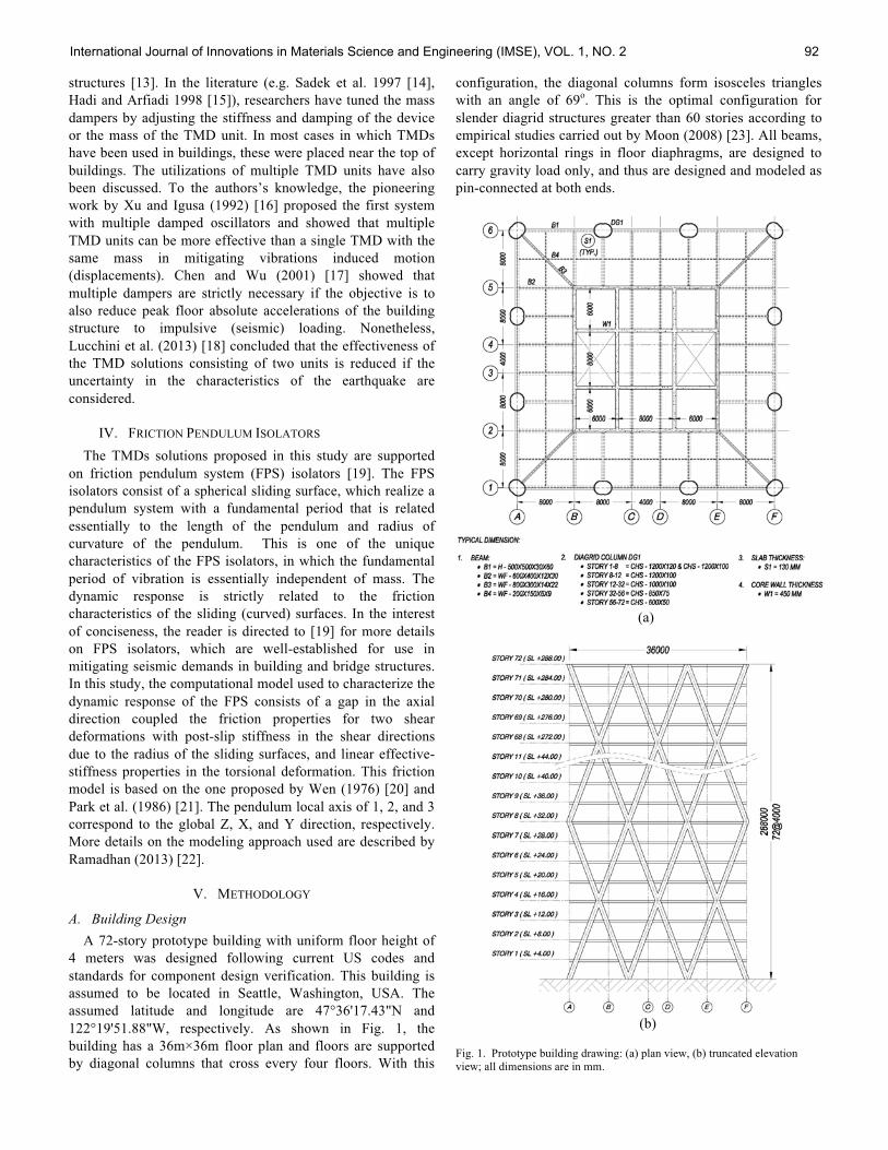
structures [13]. In the literature (e.g. Sadek et al. 1997 [14],
Hadi and Arfiadi 1998 [15]), researchers have tuned the mass
dampers by adjusting the stiffness and damping of the device
or the mass of the TMD unit. In most cases in which TMDs
have been used in buildings, these were placed near the top of
buildings. The utilizations of multiple TMD units have also
been discussed. To the authors’s knowledge, the pioneering
work by Xu and Igusa (1992) [16] proposed the first system
with multiple damped oscillators and showed that multiple
TMD units can be more effective than a single TMD with the
same mass in mitigating vibrations induced motion
(displacements). Chen and Wu (2001) [17] showed that
multiple dampers are strictly necessary if the objective is to
also reduce peak floor absolute accelerations of the building
structure to impulsive (seismic) loading. Nonetheless,
Lucchini et al. (2013) [18] concluded that the effectiveness of
the TMD solutions consisting of two units is reduced if the
uncertainty in the characteristics of the earthquake are
considered.
IV. FRICTION PENDULUM ISOLATORS
The TMDs solutions proposed in this study are supported
on friction pendulum system (FPS) isolators [19]. The FPS
isolators consist of a spherical sliding surface, which realize a
pendulum system with a fundamental period that is related
essentially to the length of the pendulum and radius of
curvature of the pendulum. This is one of the unique
characteristics of the FPS isolators, in which the fundamental
period of vibration is essentially independent of mass. The
dynamic response is strictly related to the friction
characteristics of the sliding (curved) surfaces. In the interest
of conciseness, the reader is directed to [19] for more details
on FPS isolators, which are well-established for use in
mitigating seismic demands in building and bridge structures.
In this study, the computational model used to characterize the
dynamic response of the FPS consists of a gap in the axial
direction coupled the friction properties for two shear
deformations with post-slip stiffness in the shear directions
due to the radius of the sliding surfaces, and linear effective-
stiffness properties in the torsional deformation. This friction
model is based on the one proposed by Wen (1976) [20] and
Park et al. (1986) [21]. The pendulum local axis of 1, 2, and 3
correspond to the global Z, X, and Y direction, respectively.
More details on the modeling approach used are described by
Ramadhan (2013) [22].
V. METHODOLOGY
A. Building Design
A 72-story prototype building with uniform floor height of
4 meters was designed following current US codes and
standards for component design verification. This building is
assumed to be located in Seattle, Washington, USA. The
assumed latitude and longitude are 47°36'17.43"N and
122°19'51.88"W, respectively. As shown in Fig. 1, the
building has a 36m×36m floor plan and floors are supported
by diagonal columns that cross every four floors. With this
configuration, the diagonal columns form isosceles triangles
with an angle of 69o. This is the optimal configuration for
slender diagrid structures greater than 60 stories according to
empirical studies carried out by Moon (2008) [23]. All beams,
except horizontal rings in floor diaphragms, are designed to
carry gravity load only, and thus are designed and modeled as
pin-connected at both ends.
(a)
(b)
Fig. 1. Prototype building drawing: (a) plan view, (b) truncated elevation
view; all dimensions are in mm.
International Journal of Innovations in Materials Science and Engineering (IMSE), VOL. 1, NO. 2 92

A two staged design and design verification was performed:
(1) In a first stage, the building was designed not considering
the effects of the TMDs. Models of the building were
developed and dimensions of all components of the building
were first estimated using engineering judgment. Final
dimensions were obtained through an iterative design process,
in which the forces and displacements in the building were
obtained using the response spectrum method for the
prototype building (without the TMD units); (2) In a second
stage of the design, the friction TMD system was incorporated
to the model and design obtained in the previous model. In
this second stage, nonlinear models were considered for the
TMD units, and therefore the response spectrum method was
not valid for use. Instead, nonlinear time-history response
analysis was performed as described next in this methodology
section. It is worth noting that the finite element models used
are also described next.
B. TMD Unit Design
The TMD units consist of a concrete container with sand or
water inside it, which is connected to the main structure using
friction pendulum isolators. A similar concept to the one
proposed herein can be found in One Wall Centre Hotel in
Vancouver, Canada, which holds a tuned water damping
system at the top level of the building [10]. The volume of
sand or water can be adjusted according to optimal mass
obtained from modeling and analysis. The reference model has
the friction TMD unit placed at story 68 to alleviate the
response from the first mode of the structure as shown in Fig.
2a.
(a) (b) (c)
Fig. 2. Mode shapes of the original structure and mass dampers placement:
(a) Mode 1 and solution with only one TMD unit, (b) Mode 2 and solutions
with two TMD units, (c) Mode 3.
The top friction TMD unit extends from story 68 to story 72
to provide improved load transfer from the mass damper to the
stiffer floors, that is, floors at which the diagonal columns of
the diagrid cross. It also serves as a room for the additional
required mass that is provided by the sand or water. This TMD
unit is illustrated in Fig. 3. For the model with two friction
TMD units, the first unit is the same as the reference model,
while the second is placed at story 32, extending to story 34.
The second TMD unit is illustrated in Fig. 4. Implementing
the second mass damper unit aims at reducing the contribution
of the second lateral mode of vibration (see Fig. 2). Due to the
usual shape of the seismic design response spectrum (as well
as the shape of the response spectra of the ground motions
considered) base shear forces due to the second mode (or even
the third mode) have significant contributions to the floor
accelerations and to the total base shear, as confirmed in the
results section.
(a)
(b)
Fig. 3. First TMD unit: (a) plan view at story 69 to 71, (b) cross section 1-1.
All dimensions are in mm.
Protective shock absorbers (rubber bearings or an
equivalent system) are placed between the outer horizontal
rings of the exterior diagrid and the TMD units. These
bearings are also placed between the TMD units and the inner
reinforced-concrete core. In the reference model, the TMD
unit (at story 68) has absorbers – with thickness of 1 meter –
placed in stories 69, 70, and 71. Initial gaps of 500 mm are
provided, and absorbers are only engaged after the gaps are
closed. For the model with double TMD units, the second
TMD unit (at story 32) has absorbers – with thickness of 1.5
International Journal of Innovations in Materials Science and Engineering (IMSE), VOL. 1, NO. 2 93

meters – placed at story 33. The second absorbers do not have
gaps. This allows for tuning of the period of the second mass
damper to be close to the second mode of the building.
Absorbers are also placed above the container to prevent
impact due to overturning. Lastly, additional stiff truss beams
are provided at the floor below the TMD units, to transfer the
vertical loads directly to the inner core. The design of the
braces was done to ensure that the solution was possible.
(a)
(b)
Fig. 4. Second TMD unit: (a) plan view at story 33, (b) cross section 3-3. All
dimensions are in mm.
C. Ground Motion Selection
The selection and scaling of horizontal component ground
motion acceleration time histories are crucial to produce
meaningful results and adequate comparisons of the responses
of structures subjected to these ground motions. The selection
performed herein has the primary objective of producing
acceleration histories which are consistent with the seismic
hazard at the site.
Seven (7) crustal earthquakes, listed in Table I, were chosen
and scaled from the 2011 PEER Ground Motion Database.
The target spectrum is based on ASCE 7-10 [24] with design
earthquake spectral response acceleration parameters, Sds =
0.911g, Sd1 = 0.529g, and TL = 6 sec. The target design
response spectrum is shown in Fig. 5 and Fig. 6. The Pacific
Earthquake Engineering Research Center (PEER) Center
makes a ground motion database available and has a web tool
linked to it for selection and scaling of acceleration time
histories [25]. In the selection of the earthquake records, some
parameters have to be input in the web tool. Readers are
referred to the PEER manual for details on all the variables
described next. The range of earthquake moment magnitudes
is set to Mw = 6 to 7.25. D5-95, which is the time duration for
the intensity to rise from 5% to 95% is set to 0 to 300 seconds.
Joyner-Boore distance (R_JB) and the rupture distance (Rrup)
is set to 0 to 20.5 km. The range of average shear wave
velocity in the top 30 m of soil (Vs30) is set to 190 to 350 m/s.
The scale factor, for linear scaling of the ground motion
records, is limited to 1/3 to 3.0. Lastly, the root-mean-squared
errors (RMSE) between the ASCE7-10 target response spectra
and the geometric mean of 5%-damped linear response spectra
obtained for two orthogonal directions are used as a measure
of goodness-of-fit. The RMSE are assessed in periods ranging
between 1.0 second and 10 seconds, which covers a range
below 0.2 and 1.5 of the fundamental period of the building
structures analyzed herein. Fig. 5 shows the target spectrum as
well as geometric mean of the selected response spectra of
scaled acceleration time histories. The records selected for the
crustal shallow motions are listed in Table I. It is worth noting
that these records have the lowest root-mean-squared errors
between the target response spectra and the response spectra
of all ground motion records, and had the lowest usable
frequency with a maximum value of 0.12 Hz (8.33 s).
Fig. 5. Input parameter for selecting and scaling the earthquake time series in
PEER ground motion database.
Seven (7) subductions earthquakes, shown in Table II, were
chosen and scaled from Japan [26] using the method described
in [27]. Those 7 earthquake records are obtained from the
“2011 Tohoku Earthquake” of March 11, 2011. The response
spectra for all selected earthquakes are shown in Fig. 6. It is
International Journal of Innovations in Materials Science and Engineering (IMSE), VOL. 1, NO. 2 94

worth noting that prior to this earthquake event, only very
limited data was available for large magnitude earthquake
motions, especially for the very large period range of interest
of the building structure in analysis. Thus, all motions were
selected from a single earthquake event, which may induce
some bias in the results. From the database of Japanese ground
motions used, there are a very small number of records that
could be used for the analysis in this study due to the very
large fundamental period of the tall structures. A minimum
value for the lowest useable frequency was set to 0.12 Hz
(highest useable period is T = 8.33 s), which allows for
analyzing these tall building structures will a large degree of
confidence. Often, two different components of the same
earthquake need to be filtered using different corner
frequencies. Thus, the records shown in Table II are applied to
the two horizontal directions of the building, which was the
basis for selection of the ground motions. Finally, it is worth
noting that the records for the subduction earthquakes chosen
herein have larger RMSE than the shallow crustal motions.
TABLE I
Properties of selected crustal earthquake records obtained from [25].
Event
Imperial
Valley-
06
Imperial
Valley-
06
Duzce-
Turkey
Imperial
Valley-
06
Northrid
ge-01
Imperial
Valley-
06
Northrid
ge-01
Year 1979 1979 1999 1979 1994 1979 1994
StationEl Centro
Array #8
Brawley
AirportDuzce
El Centro
Array
#10
Newhall
- W Pico
Canyon Rd.
Parachute
Test Site
Newhall
- Fire Sta
NGA# 183 161 1605 173 1045 187 1044
Scale
Factor1.194 1.986 0.743 1.479 0.906 2.000 0.911
RMSE 0.015 0.027 0.039 0.046 0.248 0.267 0.271
Pulse
(FN/FP)Yes/No Yes/No No/Yes Yes/Yes Yes/Yes No/No Yes/No
Tp
(FN/FP)
*
5.4 / -- 4 / -- -- / 5.6 4.5 / 2 2.4 / 2.2 -- / -- 2.2 / --
Magnitu
de6.53 6.53 7.14 6.53 6.69 6.53 6.69
Mechani
sm
Strike-
Slip
Strike-
Slip
Strike-
Slip
Strike-
SlipReverse
Strike-
SlipReverse
Rrup
(km)3.9 10.4 6.6 6.2 5.5 12.7 5.9
Corner
Freq**0.12 0.12 0.1 0.12 0.12 0.12 0.12
*TP is pulse period in seconds as defined by Baker (2007) [28].
*lowest usable frequency.
TABLE II
Properties of selected subduction zone earthquake records obtained from [26].
Event
Tohoku
Earthqua
ke
Tohoku
Earthqu
ake
Tohoku
Earthq
uake
Tohoku
Earthqu
ake
Tohoku
Earthqu
ake
Tohoku
Earthqu
ake
Tohoku
Earthqu
ake
DateMarch 11,
2011
March
11, 2011
March
11, 2011
March
11, 2011
March
11, 2011
March
11, 2011
March
11, 2011
Station
1103111446-
AOMH16
-EW-
Surface
1103111446-
FKSH10
-EW-
Surface
1103111446-
FKSH16
-NS-
Surface
1103111446-
FKSH20
-EW-
Surface
1103111446-
IWTH11
-NS-
Surface
1103111446-
IWTH24
-NS-
Surface
1103111446-
TCGH1
6-NS-
Surface
File
Name
AOMH16
EW2
FKSH10
EW2
FKSH16
NS2
FKSH20
EW2
IWTH11
NS2
IWTH24
NS2
TCGH1
6NS2
Scale
Factor3.000 3.000 3.000 1.252 3.000 2.806 1.573
RMSE 0.606 0.520 0.667 0.823 0.778 0.173 0.356
Magnit
ude9.000 9.000 9.000 9.000 9.000 9.000 9.000
Corner
Freq0.120 0.120 0.120 0.100 0.080 0.090 0.100
(a) (b)
(c) (d)
Fig. 6. Response spectrum of each tested ground motions: (a) crustal – fault
normal applied in X-dir, (b) crustal – fault parallel applied in Y-dir, (c)
subduction – applied in X-dir, (d) subduction – applied in Y-dir; straight line
legend: (i) without TMD [–], (ii) reference model (with TMD) [- - -], (iii) with
double TMD units [···].
D. Modeling
Structural modeling corresponds to the creation of a
mathematical model that can be solved and analyzed. In this
paper, SAP2000 [29] is the software used to analyze all
building structural models. Sap2000 uses the finite element
method to model all structural elements in the building. The
diagrid structure is modeled using linear elastic frame
elements with geometric and mechanical properties defined
based on Fig. 1a. The inner reinforced concrete wall core is
modeled using linear elastic shell elements. The effective
Young’s modulus of the walls is taken as 35% of the nominal
concrete modulus Ec. Floor diaphragms consist of a grid of
steel beams supporting a concrete slab, which are modeled as
rigid diaphragms for lateral loading. The effective Young’s
modulus of the floor slabs are taken as 25% of the nominal
concrete modulus in accordance to ACI 318-11 [30] section
10.10.4.1. Additional plan eccentricities in this regular
prototype structure were not explicitly considered. The
SAP2000 model of the prototype building consists of 8536
frame elements, 60275 joints, and 57624 shell elements. The
total number of degrees of freedom in the model is exceeds
360,000.
For modeling purposes, the concrete container (with its
content) is represented by a single wall, which is placed at
mid-distance between the outer diagrid and the inner core. The
single wall is modeled as linear elastic shell elements with
thickness and mass defined as to represent the container and
its content. It should be noted that sloshing effects of the water
surface is neglected as it will not have a considerable effect in
International Journal of Innovations in Materials Science and Engineering (IMSE), VOL. 1, NO. 2 95
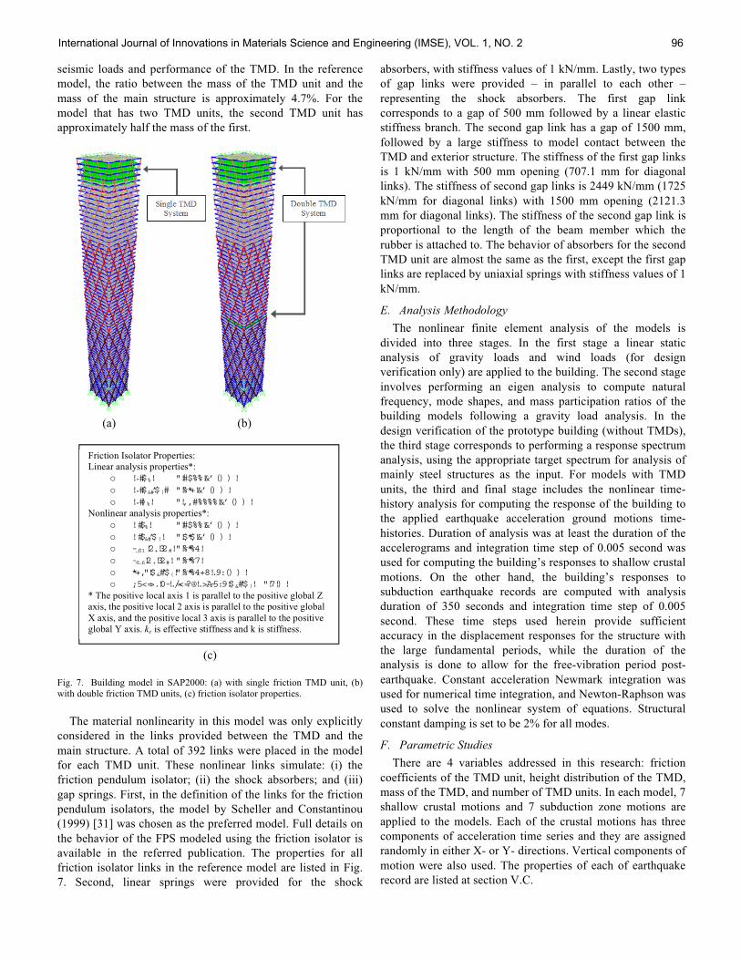
seismic loads and performance of the TMD. In the reference
model, the ratio between the mass of the TMD unit and the
mass of the main structure is approximately 4.7%. For the
model that has two TMD units, the second TMD unit has
approximately half the mass of the first.
(a) (b)
(c)
Fig. 7. Building model in SAP2000: (a) with single friction TMD unit, (b)
with double friction TMD units, (c) friction isolator properties.
The material nonlinearity in this model was only explicitly
considered in the links provided between the TMD and the
main structure. A total of 392 links were placed in the model
for each TMD unit. These nonlinear links simulate: (i) the
friction pendulum isolator; (ii) the shock absorbers; and (iii)
gap springs. First, in the definition of the links for the friction
pendulum isolators, the model by Scheller and Constantinou
(1999) [31] was chosen as the preferred model. Full details on
the behavior of the FPS modeled using the friction isolator is
available in the referred publication. The properties for all
friction isolator links in the reference model are listed in Fig.
7. Second, linear springs were provided for the shock
absorbers, with stiffness values of 1 kN/mm. Lastly, two types
of gap links were provided – in parallel to each other –
representing the shock absorbers. The first gap link
corresponds to a gap of 500 mm followed by a linear elastic
stiffness branch. The second gap link has a gap of 1500 mm,
followed by a large stiffness to model contact between the
TMD and exterior structure. The stiffness of the first gap links
is 1 kN/mm with 500 mm opening (707.1 mm for diagonal
links). The stiffness of second gap links is 2449 kN/mm (1725
kN/mm for diagonal links) with 1500 mm opening (2121.3
mm for diagonal links). The stiffness of the second gap link is
proportional to the length of the beam member which the
rubber is attached to. The behavior of absorbers for the second
TMD unit are almost the same as the first, except the first gap
links are replaced by uniaxial springs with stiffness values of 1
kN/mm.
E. Analysis Methodology
The nonlinear finite element analysis of the models is
divided into three stages. In the first stage a linear static
analysis of gravity loads and wind loads (for design
verification only) are applied to the building. The second stage
involves performing an eigen analysis to compute natural
frequency, mode shapes, and mass participation ratios of the
building models following a gravity load analysis. In the
design verification of the prototype building (without TMDs),
the third stage corresponds to performing a response spectrum
analysis, using the appropriate target spectrum for analysis of
mainly steel structures as the input. For models with TMD
units, the third and final stage includes the nonlinear time-
history analysis for computing the response of the building to
the applied earthquake acceleration ground motions time-
histories. Duration of analysis was at least the duration of the
accelerograms and integration time step of 0.005 second was
used for computing the building’s responses to shallow crustal
motions. On the other hand, the building’s responses to
subduction earthquake records are computed with analysis
duration of 350 seconds and integration time step of 0.005
second. These time steps used herein provide sufficient
accuracy in the displacement responses for the structure with
the large fundamental periods, while the duration of the
analysis is done to allow for the free-vibration period post-
earthquake. Constant acceleration Newmark integration was
used for numerical time integration, and Newton-Raphson was
used to solve the nonlinear system of equations. Structural
constant damping is set to be 2% for all modes.
F. Parametric Studies
There are 4 variables addressed in this research: friction
coefficients of the TMD unit, height distribution of the TMD,
mass of the TMD, and number of TMD units. In each model, 7
shallow crustal motions and 7 subduction zone motions are
applied to the models. Each of the crustal motions has three
components of acceleration time series and they are assigned
randomly in either X- or Y- directions. Vertical components of
motion were also used. The properties of each of earthquake
record are listed at section V.C.
Friction Isolator Properties:
Linear analysis properties*:
o !"#$%! "!#$%%!&’() ) !o !"#$&#’$(# "!%*+!&’() ) !o !"#)%! "!,,#%%%%!&’() ) !
Nonlinear analysis properties*:
o !#$%! "!#$%%!&’() ) !o !#$&#’$(! "!$*$!&’() ) !o -./01!2+!32#!"!%*%4!o --5.6!2+!32#!"!%*%7!o *+,"!$&#’$(!"!%*%4+8!.9:() ) !o ;5<=>.!0-!./=<=?@!.>A-5:9!$&#’$(! "!7!) !
* The positive local axis 1 is parallel to the positive global Z
axis, the positive local 2 axis is parallel to the positive global
X axis, and the positive local 3 axis is parallel to the positive
global Y axis. ke is effective stiffness and k is stiffness.
International Journal of Innovations in Materials Science and Engineering (IMSE), VOL. 1, NO. 2 96
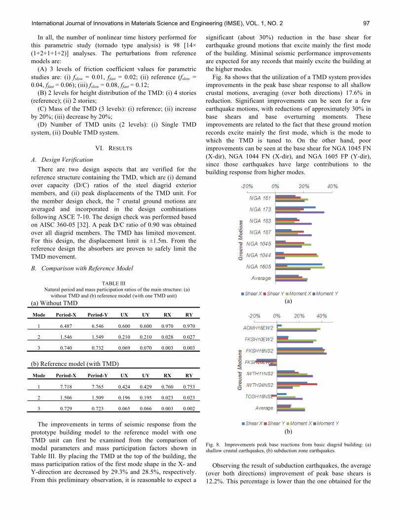
In all, the number of nonlinear time history performed for
this parametric study (tornado type analysis) is 98 [14×
(1+2+1+1+2)] analyses. The perturbations from reference
models are:
(A) 3 levels of friction coefficient values for parametric
studies are: (i) fslow = 0.01, ffast = 0.02; (ii) reference (fslow =
0.04, ffast = 0.06); (iii) fslow = 0.08, ffast = 0.12;
(B) 2 levels for height distribution of the TMD: (i) 4 stories
(reference); (ii) 2 stories;
(C) Mass of the TMD (3 levels): (i) reference; (ii) increase
by 20%; (iii) decrease by 20%;
(D) Number of TMD units (2 levels): (i) Single TMD
system, (ii) Double TMD system.
VI. RESULTS
A. Design Verification
There are two design aspects that are verified for the
reference structure containing the TMD, which are (i) demand
over capacity (D/C) ratios of the steel diagrid exterior
members, and (ii) peak displacements of the TMD unit. For
the member design check, the 7 crustal ground motions are
averaged and incorporated in the design combinations
following ASCE 7-10. The design check was performed based
on AISC 360-05 [32]. A peak D/C ratio of 0.90 was obtained
over all diagrid members. The TMD has limited movement.
For this design, the displacement limit is ±1.5m. From the
reference design the absorbers are proven to safely limit the
TMD movement.
B. Comparison with Reference Model
TABLE III
Natural period and mass participation ratios of the main structure: (a)
without TMD and (b) reference model (with one TMD unit)
(a) Without TMD
Mode Period-X Period-Y UX UY RX RY
1 6.487 6.546 0.600 0.600 0.970 0.970
2 1.546 1.549 0.210 0.210 0.028 0.027
3 0.740 0.732 0.069 0.070 0.003 0.003
(b) Reference model (with TMD)
Mode Period-X Period-Y UX UY RX RY
1 7.718 7.765 0.424 0.429 0.760 0.753
2 1.506 1.509 0.196 0.195 0.023 0.023
3 0.729 0.723 0.065 0.066 0.003 0.002
The improvements in terms of seismic response from the
prototype building model to the reference model with one
TMD unit can first be examined from the comparison of
modal parameters and mass participation factors shown in
Table III. By placing the TMD at the top of the building, the
mass participation ratios of the first mode shape in the X- and
Y-direction are decreased by 29.3% and 28.5%, respectively.
From this preliminary observation, it is reasonable to expect a
significant (about 30%) reduction in the base shear for
earthquake ground motions that excite mainly the first mode
of the building. Minimal seismic performance improvements
are expected for any records that mainly excite the building at
the higher modes.
Fig. 8a shows that the utilization of a TMD system provides
improvements in the peak base shear response to all shallow
crustal motions, averaging (over both directions) 17.6% in
reduction. Significant improvements can be seen for a few
earthquake motions, with reductions of approximately 30% in
base shears and base overturning moments. These
improvements are related to the fact that these ground motion
records excite mainly the first mode, which is the mode to
which the TMD is tuned to. On the other hand, poor
improvements can be seen at the base shear for NGA 1045 FN
(X-dir), NGA 1044 FN (X-dir), and NGA 1605 FP (Y-dir),
since those earthquakes have large contributions to the
building response from higher modes.
(a)
(b)
Fig. 8. Improvements peak base reactions from basic diagrid building: (a)
shallow crustal earthquakes, (b) subduction zone earthquakes.
Observing the result of subduction earthquakes, the average
(over both directions) improvement of peak base shears is
12.2%. This percentage is lower than the one obtained for the
International Journal of Innovations in Materials Science and Engineering (IMSE), VOL. 1, NO. 2 97
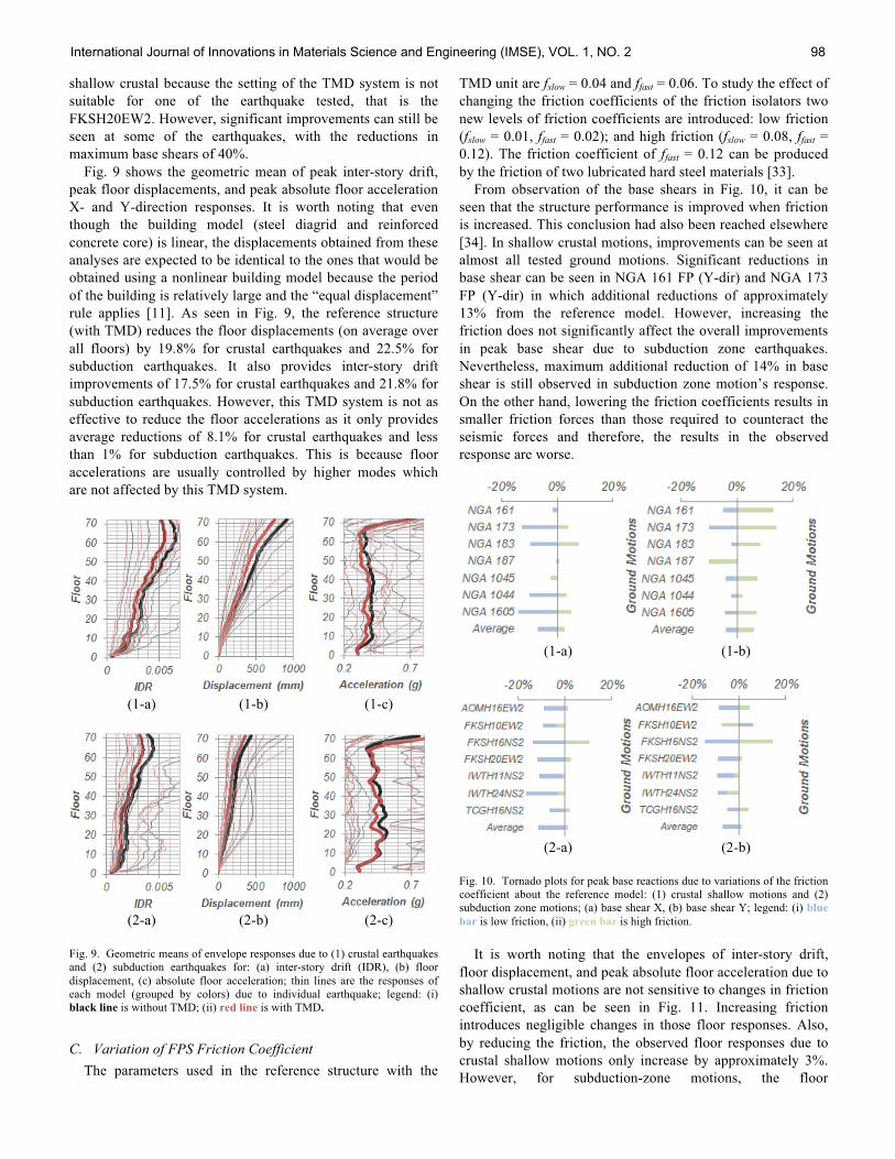
shallow crustal because the setting of the TMD system is not
suitable for one of the earthquake tested, that is the
FKSH20EW2. However, significant improvements can still be
seen at some of the earthquakes, with the reductions in
maximum base shears of 40%.
Fig. 9 shows the geometric mean of peak inter-story drift,
peak floor displacements, and peak absolute floor acceleration
X- and Y-direction responses. It is worth noting that even
though the building model (steel diagrid and reinforced
concrete core) is linear, the displacements obtained from these
analyses are expected to be identical to the ones that would be
obtained using a nonlinear building model because the period
of the building is relatively large and the “equal displacement”
rule applies [11]. As seen in Fig. 9, the reference structure
(with TMD) reduces the floor displacements (on average over
all floors) by 19.8% for crustal earthquakes and 22.5% for
subduction earthquakes. It also provides inter-story drift
improvements of 17.5% for crustal earthquakes and 21.8% for
subduction earthquakes. However, this TMD system is not as
effective to reduce the floor accelerations as it only provides
average reductions of 8.1% for crustal earthquakes and less
than 1% for subduction earthquakes. This is because floor
accelerations are usually controlled by higher modes which
are not affected by this TMD system.
(1-a) (1-b) (1-c)
(2-a) (2-b) (2-c)
Fig. 9. Geometric means of envelope responses due to (1) crustal earthquakes
and (2) subduction earthquakes for: (a) inter-story drift (IDR), (b) floor
displacement, (c) absolute floor acceleration; thin lines are the responses of
each model (grouped by colors) due to individual earthquake; legend: (i)
black line is without TMD; (ii) red line is with TMD.
C. Variation of FPS Friction Coefficient
The parameters used in the reference structure with the
TMD unit are fslow = 0.04 and ffast = 0.06. To study the effect of
changing the friction coefficients of the friction isolators two
new levels of friction coefficients are introduced: low friction
(fslow = 0.01, ffast = 0.02); and high friction (fslow = 0.08, ffast =
0.12). The friction coefficient of ffast = 0.12 can be produced
by the friction of two lubricated hard steel materials [33].
From observation of the base shears in Fig. 10, it can be
seen that the structure performance is improved when friction
is increased. This conclusion had also been reached elsewhere
[34]. In shallow crustal motions, improvements can be seen at
almost all tested ground motions. Significant reductions in
base shear can be seen in NGA 161 FP (Y-dir) and NGA 173
FP (Y-dir) in which additional reductions of approximately
13% from the reference model. However, increasing the
friction does not significantly affect the overall improvements
in peak base shear due to subduction zone earthquakes.
Nevertheless, maximum additional reduction of 14% in base
shear is still observed in subduction zone motion’s response.
On the other hand, lowering the friction coefficients results in
smaller friction forces than those required to counteract the
seismic forces and therefore, the results in the observed
response are worse.
(1-a) (1-b)
(2-a) (2-b)
Fig. 10. Tornado plots for peak base reactions due to variations of the friction
coefficient about the reference model: (1) crustal shallow motions and (2)
subduction zone motions; (a) base shear X, (b) base shear Y; legend: (i) blue
bar is low friction, (ii) green bar is high friction.
It is worth noting that the envelopes of inter-story drift,
floor displacement, and peak absolute floor acceleration due to
shallow crustal motions are not sensitive to changes in friction
coefficient, as can be seen in Fig. 11. Increasing friction
introduces negligible changes in those floor responses. Also,
by reducing the friction, the observed floor responses due to
crustal shallow motions only increase by approximately 3%.
However, for subduction-zone motions, the floor
International Journal of Innovations in Materials Science and Engineering (IMSE), VOL. 1, NO. 2 98

displacements are still not sensitive to changes in the friction
coefficient, but the inter-story drift ratios and absolute floor
acceleration are quite sensitive. High friction provides
significant absolute floor acceleration reductions of 10.5%
while low friction increases the inter-story drift by 7.9%.
(1-a) (1-b) (1-c)
(2-a) (2-b) (2-c)
Fig. 11. Floor responses due to variations in friction coefficient: (1) shallow
crustal motions and (2) subduction zone motions; (a) inter-story drift, (b) floor
displacement, (c) floor absolute acceleration; legend: (i) low friction [- - -], (ii)
reference [–], (iii) high friction [! !!!! ].
D. Variation in Height Distribution and Mass of TMD Unit
As stated in the methodology section, the configuration for
the TMD system needs the mass damper to be extended for
four floors for optimal load transfer to the exterior diagrid
structure. Fig. 12 illustrates the sensitivity of base reactions
change in height and mass of the TMD unit. It can be seen
from this figure that concentration of the same mass over half
the height results in an increase in base shear forces (average
of both directions) of approximately 3.8% for shallow crustal
motions and a decrease of 1.6% in subduction zone motions
compared to the reference model. No significant changes are
observed in displacement and acceleration floor responses due
to crustal earthquakes compared to the reference model (with
one TMD unit) as ! 3% differences were observed in Fig. 13.
In subduction zone earthquake’s responses, the floor drift and
displacement also show insignificant changes, but the absolute
floor acceleration decrease by 6.0% from the reference model.
(1-a) (1-b)
(2-a) (2-b)
Fig. 12. Tornado plots for peak base reactions due to variation in height and
mass of TMD about the reference model: (1) shallow crustal motions and (2)
subduction zone motions; (a) base shear X, (b) base shear Y; legend: (i) blue
bar is decrease mass, (ii) green bar is increase mass, (iii) purple bar is
reduce height.
(1-a) (1-b) (1-c)
(2-a) (2-b) (2-c)
Fig. 13. Floor response due to variation in height and mass: (1) shallow
crustal motions and (2) subduction zone motions; (a) inter-story drift, (b) floor
displacement, (c) floor absolute acceleration; legend: (i) decrease mass [- - -],
(ii) reference [–], (iii) increase mass [! !!!! ]; reduce height [=].
International Journal of Innovations in Materials Science and Engineering (IMSE), VOL. 1, NO. 2 99

Finally, Fig. 12 also shows the results obtained by
maintaining the height and friction parameters fixed to the
values of the reference model as the mass was varied by two
levels (+20% and -20%). By reducing the mass by 20%, the
overall base shears improvements for X and Y directions due
to shallow crustal motions decrease by 3 and 5%, respectively,
compared to the reference model. On the other hand, the
average base reaction changes due to subduction zone motions
are still irregular. Nonetheless, decreasing the mass of the
TMD is still decreasing the overall base reactions
improvements compared to the reference model. Additionally,
increasing the mass by 20% corresponds to overall base shear
improvements of only 3% from the reference for shallow
crustal motions and 4% for subduction zone motions. As seen
from Fig. 13, the changes in mass are also not affecting the
displacement and acceleration floor response for shallow
crustal motions. The observed floor responses only fluctuated
by approximately 3.3%. However, the changes are reasonably
significant in subduction earthquakes. While floor
displacements do not differ much, increasing the mass by 20%
increase the overall floor absolute accelerations improvement
by 7.6% while decreasing the mass will do the contrary.
E. Comparison with Double TMD System
TABLE IV
Fundamental periods and mass participation ratios of the main structure with
double TMD system.
Mode Period-X Period-Y UX UY RX RY
1 7.727 7.775 0.427 0.431 0.761 0.754
2 1.433 1.435 0.142 0.140 0.017 0.017
3 0.728 0.722 0.065 0.066 0.003 0.002
Fig. 14. Mode shapes and mass participation ratios of each mass damper in
the two models.
The modal parameters and mass participation factors are
still useful to estimate the expected improvements in terms of
seismic response of the model with the double TMD system.
TABLE IV lists the three main periods of vibration of the
structure in the X- and Y-direction. Fig. 14 shows the mode
shapes and mass participation ratios of each mass damper in
the double TMD system in comparison the single TMD
system (reference model). It can be seen that for the model
with the additional TMD in story 32, the mass participation of
the first mode increases slightly, while a decrease of the mass
participation ratio for the second mode is observed. It is clear,
that the inclusion of the second TMD unit influences mainly
the participation of the second mode, and thus this TMD unit
is said to be tuned for the second mode only.
(a)
(b)
Fig. 15. Improvements in peak base reactions of double TMD system from
reference model (single TMD system) due to: (a) shallow crustal motions, (b)
subduction zone motions.
Fig. 15 shows that the utilization of double TMD system
results in improvements in the peak base shear responses for
almost all tested ground motions. For the shallow crustal
motions, the double TMD system gives additional
improvements of 5.7% to peak base shear responses
(averaging in both directions) over the reference model and
also resulting in a reduction of 23.3% of total peak base shear
reduction. Significant improvements are observed for NGA
161 FP, NGA 173 FP, and NGA 183 FP with approximately
15% of additional improvements in peak base shear over the
reference model. In the response generated by subduction zone
motions, a similar trend is observed. The double TMD system
reduce the overall peak base shear responses by 6.0% with
maximum reduction of approximately 20%. However, for one
particular earthquake, that is FKSH20EW2, although the
International Journal of Innovations in Materials Science and Engineering (IMSE), VOL. 1, NO. 2 100
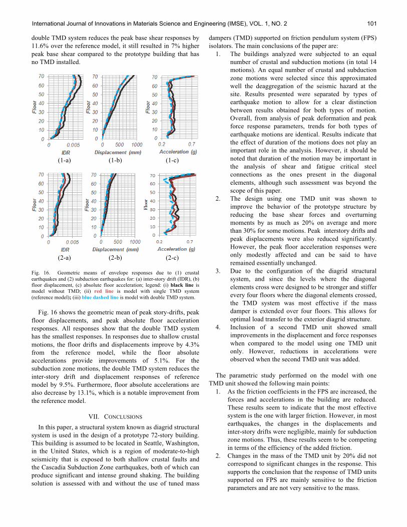
double TMD system reduces the peak base shear responses by
11.6% over the reference model, it still resulted in 7% higher
peak base shear compared to the prototype building that has
no TMD installed.
(1-a) (1-b) (1-c)
(2-a) (2-b) (2-c)
Fig. 16. Geometric means of envelope responses due to (1) crustal
earthquakes and (2) subduction earthquakes for: (a) inter-story drift (IDR), (b)
floor displacement, (c) absolute floor acceleration; legend: (i) black line is
model without TMD; (ii) red line is model with single TMD system
(reference model); (iii) blue dashed line is model with double TMD system.
Fig. 16 shows the geometric mean of peak story-drifts, peak
floor displacements, and peak absolute floor acceleration
responses. All responses show that the double TMD system
has the smallest responses. In responses due to shallow crustal
motions, the floor drifts and displacements improve by 4.3%
from the reference model, while the floor absolute
accelerations provide improvements of 5.1%. For the
subduction zone motions, the double TMD system reduces the
inter-story drift and displacement responses of reference
model by 9.5%. Furthermore, floor absolute accelerations are
also decrease by 13.1%, which is a notable improvement from
the reference model.
VII. CONCLUSIONS
In this paper, a structural system known as diagrid structural
system is used in the design of a prototype 72-story building.
This building is assumed to be located in Seattle, Washington,
in the United States, which is a region of moderate-to-high
seismicity that is exposed to both shallow crustal faults and
the Cascadia Subduction Zone earthquakes, both of which can
produce significant and intense ground shaking. The building
solution is assessed with and without the use of tuned mass
dampers (TMD) supported on friction pendulum system (FPS)
isolators. The main conclusions of the paper are:
1. The buildings analyzed were subjected to an equal
number of crustal and subduction motions (in total 14
motions). An equal number of crustal and subduction
zone motions were selected since this approximated
well the deaggregation of the seismic hazard at the
site. Results presented were separated by types of
earthquake motion to allow for a clear distinction
between results obtained for both types of motion.
Overall, from analysis of peak deformation and peak
force response parameters, trends for both types of
earthquake motions are identical. Results indicate that
the effect of duration of the motions does not play an
important role in the analysis. However, it should be
noted that duration of the motion may be important in
the analysis of shear and fatigue critical steel
connections as the ones present in the diagonal
elements, although such assessment was beyond the
scope of this paper.
2. The design using one TMD unit was shown to
improve the behavior of the prototype structure by
reducing the base shear forces and overturning
moments by as much as 20% on average and more
than 30% for some motions. Peak interstory drifts and
peak displacements were also reduced significantly.
However, the peak floor acceleration responses were
only modestly affected and can be said to have
remained essentially unchanged.
3. Due to the configuration of the diagrid structural
system, and since the levels where the diagonal
elements cross were designed to be stronger and stiffer
every four floors where the diagonal elements crossed,
the TMD system was most effective if the mass
damper is extended over four floors. This allows for
optimal load transfer to the exterior diagrid structure.
4. Inclusion of a second TMD unit showed small
improvements in the displacement and force responses
when compared to the model using one TMD unit
only. However, reductions in accelerations were
observed when the second TMD unit was added.
The parametric study performed on the model with one
TMD unit showed the following main points:
1. As the friction coefficients in the FPS are increased, the
forces and accelerations in the building are reduced.
These results seem to indicate that the most effective
system is the one with larger friction. However, in most
earthquakes, the changes in the displacements and
inter-story drifts were negligible, mainly for subduction
zone motions. Thus, these results seem to be competing
in terms of the efficiency of the added friction.
2. Changes in the mass of the TMD unit by 20% did not
correspond to significant changes in the response. This
supports the conclusion that the response of TMD units
supported on FPS are mainly sensitive to the friction
parameters and are not very sensitive to the mass.
International Journal of Innovations in Materials Science and Engineering (IMSE), VOL. 1, NO. 2 101
In summary, this document presented a design example and
a TMD solution which can be incorporated into the design
of a tall building using diagrid steel structures.
ACKNOWLEDGMENT
The Authors would like to acknowledge the support of the
School of Civil and Construction Engineering at Oregon State
University.
REFERENCES
[1] M. M. Ali and K. S. Moon, “Structural developments in tall buildings:
current trends and future prospects,” Archit. Sci. Rev., vol. 50, no. 3, pp.
205–223, 2007.
[2] Council on Tall Buildings and Urban Habitat, “The Global Tall
Building Database of the CTBUH,” The Skyscraper Center, 2014.
[Online]. Available: http://www.skyscrapercenter.com/.
[3] I. McCain, “Diagrid: Structural Efficiency & Increasing Popularity.”
[4] S. L. Kramer, Geotechnical earthquake engineering. in prentice–Hall
international series in civil engineering and engineering mechanics.
Prentice-Hall, New Jersey, 1996.
[5] K. Romney, “Soil-Bridge Interaction during Long-Duration Earthquake
Motions,” Master’s Thesis, Oregon State University, Corvallis, Oregon,
2013.
[6] Arup, “Sony City, Tokyo: A Diagrid Combined with Base Isolation,”
Arup J., vol. 2, pp. 49–51, 2009.
[7] A. Wada and N. Mori, “Seismic Design for the Sustainable City: A
Report on Japanese Practice,” in Structures Congress 2008, American
Society of Civil Engineers, pp. 1–8.
[8] A. Lago, T. J. Sullivan, and G. M. Calvi, “A novel seismic design
strategy for structures with complex geometry,” J. Earthq. Eng., vol. 14,
no. S1, pp. 69–105, 2010.
[9] M. C. Constantinou and I. G. Tadjbakhsh, “Optimum characteristics of
isolated structures,” J. Struct. Eng., vol. 111, no. 12, pp. 2733–2750,
1985.
[10] Glotman Simpson, “Project Showcase - One Wall Centre,” Glotman
Simpson Consulting Engineers, 2001. [Online]. Available:
http://www.glotmansimpson.com/Commercial/One-Wall-Centre.
[Accessed: 03-Nov-2013].
[11] A. K. Chopra, Dynamics of structures: Theory and applications to
earthquake engineering, 2nd ed. Saddle River: Prentice Hall, 2001.
[12] J. A. Inaudi and J. M. Kelly, “A friction mass damper for vibration
control,” Earthquake Engineering Research Center, University of
California, Berkeley, California, UCB/EERC-92/15, 1992.
[13] P. H. Wirsching and G. W. Campbell, “Minimal structural response
under random excitation using the vibration absorber,” Earthq. Eng.
Struct. Dyn., vol. 2, no. 4, pp. 303–312, 1973.
[14] F. Sadek, B. Mohraz, A. W. Taylor, and R. M. Chung, “A method of
estimating the parameters of tuned mass dampers for seismic
applications,” Earthq. Eng. Struct. Dyn., vol. 26, no. 6, pp. 617–636,
1997.
[15] M. N. Hadi and Y. Arfiadi, “Optimum design of absorber for MDOF
structures,” J. Struct. Eng., vol. 124, no. 11, pp. 1272–1280, 1998.
[16] K. Xu and T. Igusa, “Dynamic characteristics of multiple substructures
with closely spaced frequencies,” Earthq. Eng. Struct. Dyn., vol. 21, no.
12, pp. 1059–1070, 1992.
[17] G. Chen and J. Wu, “Optimal placement of multiple tune mass dampers
for seismic structures,” J. Struct. Eng., vol. 127, no. 9, pp. 1054–1062,
2001.
[18] A. Lucchini, R. Greco, G. C. Marano, and G. Monti, “Robust Design of
Tuned Mass Damper Systems for Seismic Protection of Multistory
Buildings,” J. Struct. Eng., 2013.
[19] G. Mosqueda, A. S. Whittaker, and G. L. Fenves, “Characterization and
modeling of friction pendulum bearings subjected to multiple
components of excitation,” J. Struct. Eng., vol. 130, no. 3, pp. 433–442,
2004.
[20] Y.-K. Wen, “Method for random vibration of hysteretic systems,” J.
Eng. Mech. Div., vol. 102, no. 2, pp. 249–263, 1976.
[21] Y. J. Park, Y. K. Wen, and A. Ang, “Random vibration of hysteretic
systems under bi-directional ground motions,” Earthq. Eng. Struct.
Dyn., vol. 14, no. 4, pp. 543–557, 1986.
[22] G. Ramadhan, “Seismic performance of diagrid steel structures using
single and double friction mass dampers,” Master’s Thesis, Oregon
State University, Corvallis, Oregon, 2013.
[23] K. S. Moon, “Optimal grid geometry of diagrid structures for tall
buildings,” Archit. Sci. Rev., vol. 51, no. 3, pp. 239–251, 2008.
[24] American Society of Civil Engineers, Minimum design loads for
buildings and other structures. Virginia: ASCE, 2010.
[25] PEER, “2011 PEER Ground Motion Database – Beta Version,” PEER
Ground Motion Database, 2011. [Online]. Available:
http://peer.berkeley.edu/peer_ground_motion_database/spectras/new.
[Accessed: 20-Aug-2013].
[26] National Research Institute for Earth Science and Disaster Prevention,
“Strong-Motion Seismograph Networks.” [Online]. Available:
http://www.k-net.bosai.go.jp. [Accessed: 03-Feb-2013].
[27] A. R. Barbosa, H. B. Mason, and K. Romney, “SSI-Bridge: Solid-
Bridge Interaction During Long-Duration Earthquake Motions,”
University of Washington, Seattle, WA, USDOT University
Transportation Center for Federal Region 10, PacTrans Report, 2014.
[28] J. W. Baker, “Quantitative classification of near-fault ground motions
using wavelet analysis,” Bull. Seismol. Soc. Am., vol. 97, no. 5, pp.
1486–1501, 2007.
[29] Computer and Structures, SAP2000 v15.1.0. Berkeley: Computer and
Structures, 2011.
[30] A. C. I. Committee, “Building code requirements for structural concrete
(318-11) and commentary-(318R-11),” Detroit Mich. Am. Concr. Inst.,
2011.
[31] J. Scheller and M. C. Constantinou, “Response history analysis of
structures with seismic isolation and energy dissipation systems:
verification examples for Program SAP2000,” Tech. Rep. MCEER, no.
99–0002, 1999.
[32] B. ANSI, “AISC 360-05-Specification for Structural Steel Buildings,”
Chicago! AISC, 2005.
[33] R. Ramsdale, “Reference Tables - Coefficient of Friction,” Engineer’s
Handbook. [Online]. Available:
http://www.engineershandbook.com/Tables/frictioncoefficients.htm.
[Accessed: 20-Oct-2013].
[34] T. A. Morgan and S. A. Mahin, “The optimization of multi-stage
friction pendulum isolators for loss mitigation considering a range of
seismic hazard,” in Proceedings of the 14th World Conference on
Earthquake Engineering, Beijing, China, 2008.
International Journal of Innovations in Materials Science and Engineering (IMSE), VOL. 1, NO. 2 102


