. International Outsourcing, Exchange Rates, and Monetary Policy Wai-Ming Ho * Department of Economics York University June 2018 Abstract Firms’ decisions to outsource the production of intermediate inputs abroad depend on the macroeconomic environment set by governments’ monetary and foreign exchange policies, while the relocations of production have important implications on the liquidity demands in the financial markets, which in turn affect the policy effectiveness. This paper constructs a two-country, mone- tary model with segmented financial markets to incorporate the microeconomic foundations of firms’ make-or-buy decisions and highlight the working capital needs of both of the buyers and suppliers of intermediate inputs. The interdependence of firms’ sourcing decisions and governments’ conducts of policies are examined by identifying the endogenous adjustments of international outsourcing at both the extensive and intensive margins. It shows that the adjustments at the extensive margin can alter qualitatively the impacts of a currency revaluation and help explaining the perverse effect on the trade balance. The adjustments at the intensive margin demonstrate how firms’ sourcing decisions and payment arrangements act to dampen the effects of monetary shocks. Keywords: International Outsourcing, Liquidity Constraints, Monetary Policy, Currency Revaluation. JEL Classification: E44, F41 * Department of Economics, York University, 4700 Keele Street, Toronto, Ontario, Canada M3J 1P3 Tel: 416 736 2100 ext.22319. Fax: 416 736 5987. Email: [email protected].
Transcript
.
International Outsourcing, Exchange Rates, and Monetary Policy
Wai-Ming Ho∗
Department of Economics
York University
June 2018
Abstract
Firms’ decisions to outsource the production of intermediate inputs abroad depend on the
macroeconomic environment set by governments’ monetary and foreign exchange policies, while
the relocations of production have important implications on the liquidity demands in the financial
markets, which in turn affect the policy effectiveness. This paper constructs a two-country, mone-
tary model with segmented financial markets to incorporate the microeconomic foundations of firms’
make-or-buy decisions and highlight the working capital needs of both of the buyers and suppliers of
intermediate inputs. The interdependence of firms’ sourcing decisions and governments’ conducts
of policies are examined by identifying the endogenous adjustments of international outsourcing at
both the extensive and intensive margins. It shows that the adjustments at the extensive margin
can alter qualitatively the impacts of a currency revaluation and help explaining the perverse effect
on the trade balance. The adjustments at the intensive margin demonstrate how firms’ sourcing
decisions and payment arrangements act to dampen the effects of monetary shocks.
Keywords: International Outsourcing, Liquidity Constraints, Monetary Policy,
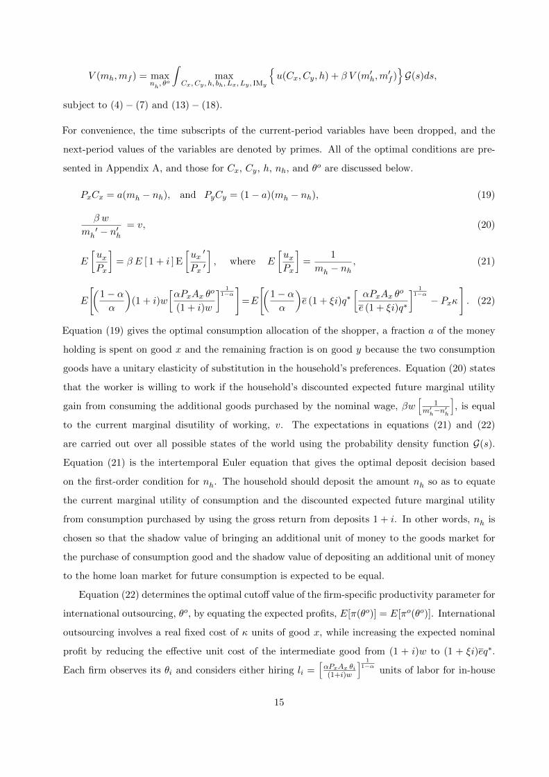
Currency Revaluation.
JEL Classification: E44, F41
∗ Department of Economics, York University, 4700 Keele Street, Toronto, Ontario, Canada M3J 1P3
International outsourcing has become an important phenomenon in globalization.1 Domestic firms
outsource to unaffiliated foreign suppliers to take advantage of lower costs of labor and intermediate
inputs abroad. The effects of these international transactions on the flows of goods and labor have
been studied extensively in the theoretical literatures on international trade and labor economics.2
However, the financial dimension of the transactions has been largely neglected; and the impli-
cations of international outsourcing for the macroeconomy and for the conducts of monetary and
foreign exchange policies have received relatively little attention. The relocation of production of
intermediate inputs affects the liquidity demands in the domestic and foreign loan markets. Mone-
tary and foreign exchange policies influence the availability of liquidity in the financial markets. It
is important for the firms to understand how these policies affect their tradeoffs between in-house
production and sourcing abroad. It is also crucial for the policymakers to recognize the impacts
of the presence of international outsourcing on the transmission channels of their policies. The
investigation of this interdependence would provide new insights into the effectiveness of monetary
policy. It also helps understanding the perverse effect of currency revaluations on the trade balance.
This paper incorporates the microeconomic foundations of firms’ make-or-buy decisions into a
two-country, monetary model with segmented financial markets to highlight two key features of
international outsourcing. First, a firm’s decision to use an imported intermediate input is optional
and sensitive to the economic environment. Second, firms’ make-or-buy decisions determine not
only the locations of production of the intermediate inputs but also the loan markets to which the
intermediate good producers seek external financing for their working capital needs.
To emphasize that outsourcing is not necessary but optional, the intermediate inputs produced
domestically and abroad are assumed to be perfect substitutes in the model. By incurring a fixed
1As reported in the World Bank’s International Trade Statistics 2013, the share of intermediate goods in worldnon-fuel exports was equal to 55% in 2011. Although the measures of international intermediate trade do not allowfor a distinction between arm’s-length and intra-firm trade, Lanz and Miroudot (2011) analyze the intra-firm tradestatistics of the United States in 2009 and report the shares of arm’s length transactions in US exports and importsof intermediate goods to be 71.3% and 51.8%, respectively.
2Spencer (2005) and Helpman (2006) survey the theoretical literature that combines trade and the organizationalchoices of firms to provide insights into the forces driving international outsourcing. A recent review of the interna-tional trade literature on multinational firms has been presented in Antras and Yeaple (2013). Feenstra and Hanson(2001) provide a detailed discussion of the impacts of trade in intermediate inputs on wages and employment. Someexamples of recent theoretical studies are Antras, Garicano, and Rossi-Hansberg (2006), Baldwin and Robert-Nicoud(2007), and Holmes and Thornton Snider (2011) analyzing the wage effects, and Keuschnigg and Ribi (2009) andKoskela and Stenbacka (2009, 2010) examining the employment effects of outsourcing.
1
cost of international outsourcing, a domestic firm can import the intermediate input at a lower
unit cost. Depending on their productivity levels in producing the final good, some domestic firms
prefer international outsourcing to producing their intermediate inputs in-house. Hence, firms’
reliance on the imported intermediate inputs is endogenously determined, the economy can adjust
its use of the imported intermediate inputs not only at the intensive margin (the changes in the
quantities demanded for imports of the firms that have already been sourcing from abroad) but also
at the extensive margin (the changes in the number of firms entering in outsourcing arrangements).
Focusing on the adjustment in the intensive margin, the model shows how the effects of temporary
monetary policy shocks are weakened by the presence of international outsourcing. Understanding
the adjustments at the extensive margin in response to permanent policy changes such as exchange
rate revaluations provides new insights into the relationship between firms’ endogenous sourcing
decisions and a country’s trade balance.
In order to highlight the impacts of international outsourcing on the demands for liquidity
in financial markets, we assume cash-in-advance constraints and segmented financial markets to
model the role of financial flows in facilitating the flows in goods and labor. The cash-in-advance
assumption highlights the liquidity services provided by money. Financial market segmentation
implies asymmetric access to liquidity by different market participants; financial intermediaries
channel funds collected from depositors to provide working capital for production and international
trade. The financial frictions are important in affecting the relative unit cost of intermediate inputs
between the two locations. Our general equilibrium framework demonstrates how the domestic
country’s output of final good is affected by the interactions of the supplies and demands of loanable
funds in both the domestic and foreign loan markets.
To keep the model simple, we assume that labor is the only primary factor of production in the
world economy, and that production fragmentation occurs in the final good sector of the domestic
country only. Domestic firms can choose between domestic in-house production or international
outsourcing. We rule out domestic outsourcing and foreign integration by construction so as to fo-
cus on the implications of firms’ make-or-buy decisions on the allocations in the labor and financial
markets of both countries.3 The outsourcing relationship involves the domestic firms outsourcing
some tasks to arm’s length firms in the foreign country, referred to as the production of the in-
termediate good for convenience. The value added by foreign labor to the domestic production is
3The assumptions that support this construction will be discussed in Section 3. The choice between in-houseproduction and domestic outsourcing has no impact on the foreign labor market. Foreign integration can affect thedomestic and foreign labor markets, but the intra-firm trade does not give rise to changes in the external financingof the buyers and suppliers of intermediate goods in the domestic and foreign financial markets.
2
therefore captured by the value of the domestic economy’s imports of intermediates.4
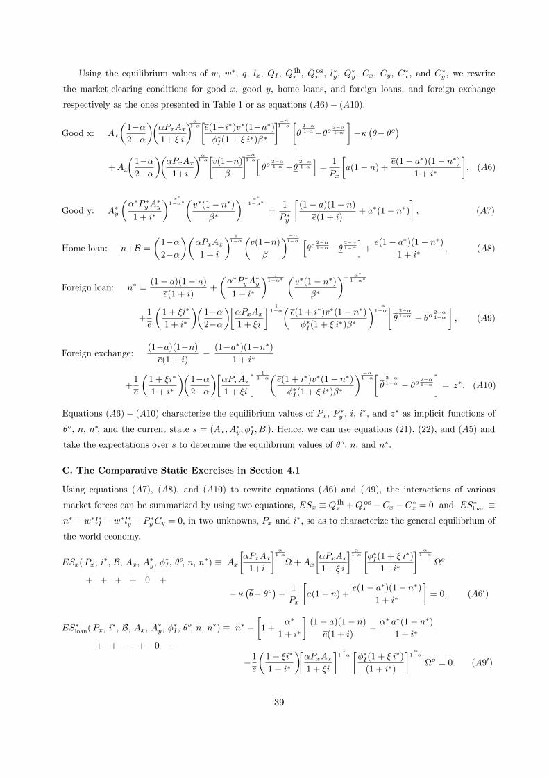
The results are summarized as follows. First, under a fixed nominal exchange rate regime, the
effects of monetary shocks depend not only on the presence of international outsourcing activities
but also on the contractual upfront payment arrangements between the domestic (source) firms and
their foreign suppliers. The domestic firms’ decisions to outsource shift the financing of the working
capital required for the production of the intermediate input from the domestic loan market to the
foreign loan market. The upfront payment arrangement determines the foreign suppliers’ reliance
on the foreign loan market in meeting their working capital needs, affecting the responsiveness
of liquidity demands to interest rates. With a low upfront payment for the intermediate input,
domestic production will be less sensitive to the liquidity shocks in the domestic loan market, so
that the effectiveness of the domestic country’s monetary policy will be dampened.
Second, a foreign currency revaluation leads more domestic firms to outsource to foreign firms
and results in an improvement in the foreign country’s trade balance. The general equilibrium
adjustment mechanism is the reason behind these counter-intuitive results. When there is no inter-
national outsourcing, an increase in the value of foreign currency results in reductions (increases)
in the domestic (foreign) households’ demands for imported consumption goods, deteriorating the
foreign country’s trade balance. With international outsourcing, there are additional effects via
the adjustments of trade in intermediates. A foreign currency revaluation leads the domestic firms
that have been outsourcing abroad to adjust at the intensive margin by reducing their intermediate
imports. As their production of the domestic consumption good decreases, the domestic price of
the domestic consumption good rises substantially, leading some domestic firms to switch from pro-
ducing their intermediate inputs in-house to outsourcing abroad. The adjustment of the imports
of intermediates at the extensive margin plays a dominant role in determining the trade flows,
resulting in a perverse effect on the trade balance.
Third, a reduction in the fixed cost associated with outsourcing makes the foreign country better
off and the domestic country worse off under both flexible and fixed exchange rate regimes. Given
that a revaluation of the foreign currency benefits the domestic country and makes the foreign
country worse off, it can be used as a policy tool to redistribute some of the welfare gain of the
foreign country to the domestic country so that both countries can benefit from a reduction in
the fixed cost of international outsourcing and attain a higher aggregate welfare level. This result
4The trade in intermediates in this model is defined in a broader sense to capture not only the trade in intermediategoods and services, but also the trade in tasks introduced by Grossman and Rossi-Hansberg (2008) to describe thevalue added contributed by the factors of production in different locations.
3
highlights the asymmetry in the welfare effects of international outsourcing and illustrates the
welfare-redistributive role of a fixed exchange rate regime when there is international outsourcing.
The remainder of the paper is organized as follows. In Section 2, we discuss the related literature
and contributions of this paper. The model is presented in Section 3. Section 4 analyzes the effects
of changes in some exogenous variables on the world economy. Some welfare analyses are presented
in Section 5. Section 6 concludes the paper.
2 Related Literature
The international trade of intermediates and vertical specialization have been modeled in the litera-
ture of open-economy macroeconomics. Kose and Yi (2001, 2006), Ambler, Cardia, and Zimmerman
(2002), Head (2002), Huang and Liu (2007), Burstein, Kurz, and Tesar (2008), and Arkolakis and
Ramanarayanan (2009) have examined the roles of intermediate input trade and vertical struc-
ture of production in the propagating mechanism of international business cycles using dynamic
stochastic general equilibrium models. Kollmann (2002), Huang and Liu (2006), and Shi and Xu
(2007) examine the optimal monetary policy in the presence of intermediate input trade. Dev-
ereux and Engel (2007) study the desirability of flexible exchange rate in a two-country model
with intermediate goods. This paper contributes to this macroeconomic literature by focusing on
trade in intermediates via international outsourcing and emphasizing the role of financial flows in
facilitating production and trade. First, the models in the literature make trade in intermediates
necessary by assuming that each type of intermediate input is produced exclusively by the firms
of one country, and that both the domestic and imported intermediates must be used in the pro-
duction of final goods.5 In contrast, this paper allows the use of the intermediate inputs to be
determined endogenously and adjusted in both the intensive and extensive margins, providing a
better understanding of the macroeconomic implications of individual firms’ intermediate input
sourcing decisions. Second, the financial aspects of the transactions are often omitted in this lit-
erature. Our study demonstrates how firms’ sourcing decisions affect the demands for liquidity in
financial markets for financing the production and trade of intermediate inputs and therefore play
an important role in the transmission of the effects of monetary and foreign exchange policies.6
5For example, Kose and Yi (2001, 2006) assume that the elasticity of substitution between domestic and foreignintermediate goods is equal to 1.5. Ambler, Cardia, and Zimmerman (2002), Devereux and Engel (2007), Huang andLiu (2007) and Shi and Xu (2007 and 2010) assume Cobb-Douglas production functions so that the domestic andforeign intermediate inputs have a unitary elasticity of substitution. Devereux and Genberg (2007) assume a Leontieftechnology that imported intermediate inputs must be used in fixed proportion with domestic inputs.
6Some recent theoretical studies of gain from multinational production focusing intra-firm trade are presentedby Bauer and Langenmayr (2013), Garetto (2013), Irarrazabal, Moxnes, and Opromolla (2013), and Ramondo and
4
Our emphasis on the financial aspects of international outsourcing also contributes to two
strands of the trade literature. First, as common in the literature on the organizational choices
of firms, following Antras and Helpman (2004), this paper models firms’ make-or-buy decisions
as a tradeoff between the fixed sourcing cost and the variable cost of intermediate inputs.7 The
investigation of the financial flows required to facilitate the flows of goods and labor illustrates how
the tradeoff is affected by the financing costs. Our examination of the financing of the contractual
upfront payments in affecting intermediate good trade in a general equilibrium framework comple-
ments the discussions of the effects of financial frictions on firms’ sourcing decisions and choices
of trade modes by Antras, Desai, and Foley (2009), Feenstra, Li, and Yu (2009), and Manova and
Yu (2012). Second, the global trade collapse during 2008-2009 has raised attention to the negative
impacts of domestic financial market frictions on firms’ ability to exports and on countries’ trade
flows.8 See Manova (2010) for a detailed survey of the literature on trade and finance. This paper
points out that the relative availability of liquidity in the domestic and foreign financial markets is
also important in determining the international trade flows when production becomes increasingly
fragmented across countries.
Some recent empirical studies find that Chinese trade flows do not respond to exchange rate
movements as suggested by conventional wisdom.9 Marquez and Schindler (2007), Thorbecke and
Smith (2010), and Cheung, Chinn, and Qian (2012) re-examine Chinese trade flows by using dis-
aggregated data. They conclude that the rapid changing economic structure may have contributed
to the unstable and perverse effects at the aggregate level. Some theoretical studies, for example,
Devereux and Genberg (2007) and Dong (2012), analyze the role of intermediate input trade in the
global imbalance adjustments and explain why a country’s trade surplus may not be responsive to
its exchange rate. However, they cannot explain China’s accelerating increases in its trade surplus
along with its currency revaluations. This study offers a theoretical framework to rationalize the
puzzling positive correlation between China’s currency value and its trade surplus. Taking into ac-
count the rise of China as a major host country of international outsourcing and considering China
as the foreign country in our model, we find that firms’ endogenous sourcing decisions are crucial in
generating different impacts of currency revaluations on the trade balances of the consumer goods
and intermediate goods and the overall trade balance. Our finding sheds light on the continuing
Rodrıguez-Clare (2013), however, macroeconomic policies do not play a role in these studies.7See Spencer (2005) and Helpman (2006) for a detailed survey of this literature.8Lanz and Miroudot (2011) find that during the period of 2008-2009, the United States experienced a larger decline
in its imports of intermediate goods than in its imports of final goods.9See Cheung, Chinn, and Qian (2012) for a detailed survey.
5
improvements in China’s trade balance in intermediate goods in spite of the substantial increases
in its currency value in recent years. In addition, the prediction of having negative welfare impacts
on its own economy, in spite of improvements in its trade balance, offers an explanation for China’s
resistance to the external pressure to revalue its currency.
3 The Model
Consider a world economy consisting of two countries, home and foreign. All foreign variables and
parameters will be indexed with asterisks (*). There are two final (consumer) goods, goods x and y,
one intermediate input, referred to as good I, and one primary factor of production, labor. In each
country, there are a monetary authority and a measure one of ex-ante identical, infinitely-lived,
multi-member households. Each household consists of five members: a shopper, an entrepreneur,
a worker, a financial intermediary, and an importer. Household members separate and conduct
different tasks in different segmented markets during a period, while pooling their income and
consumption at the end of the period.10 All markets are perfectly competitive so that everyone
acts as a price taker. To introduce money to the world economy, all transactions are subject to cash-
in-advance constraints, and payments must be made in terms of the sellers’ currency. Shoppers need
cash to pay for their consumption purchases. Entrepreneurs and importers need working capital to
facilitate their activities because of the timing frictions between the payments of operating costs
and receipts from sales. All loans are intermediated through financial intermediaries.
3.1 Preferences
The preferences of the representative home household are given by the life-time utility function,
U =∞∑t=0
β t u(Cxt, Cyt, ht), 0 < β < 1, (1)
where the instantaneous utility function u(Cxt, Cyt, ht) = a lnCxt + (1− a) lnCyt + v [ 1− ht ], and
β is the subjective discount factor. In period t, the household consumes Cjt units of final good j,
j = x, y, and supplies ht units of its worker’s labor effort to the home labor market. The expenditure
share on good x is given by the parameter a, 0 < a < 1.11 The worker’s time endowment is
normalized to one, and v is a positive parameter measuring the constant marginal utility of leisure.
10The construction of multiple-member household follows from Lucas (1990). In spite of the distinction of theagents into shoppers, entrepreneurs, workers, importers, and financial intermediaries, they pool their resources atthe end of each period, allowing for the tractability and retaining the simplicity of the representative household. Aswill be illustrated in Section 3.5, this allows the decision making of each individual member to be nested into thehousehold’s optimization problem.
11There is home bias in consumption in the case with 12< a < 1.
6
The representative foreign household has a similar utility function, U∗=∑∞t=0 β
Given the country-wide production parameters, Axt and α, and the firm-specific productivity pa-
rameter, θit, the entrepreneur inputs Iit units of intermediate good I to produce Qixt units of
good x. In each period t, the parameter θit is uniformly distributed on the unit interval [ θ, θ ],
where 0 ≤ θ < θ and θ − θ = 1.
Every home firm can produce its intermediate input domestically in-house following an identical,
linear production technology, using one unit of labor effort to produce one unit of good I.
Iit = lit, (3)
where lit is the labor input hired from the home labor market. As all home firms face the same
production technology (3), there will be no domestic outsourcing (trade in intermediates among the
home firms). However, the home firms have the option to import good I from the foreign country
by engaging in international outsourcing, facing the unit cost of q∗t units of foreign currency plus a
real fixed cost of international outsourcing, κ units of good x.12
Each home firm is subject to a cash-in-advance constraint, it has to borrow its working capital
from a home financial intermediary to finance its operation (hiring domestic workers or importing
good I) in order to maximize its profit. It is noted that the decreasing returns production technology
given by (2) can be interpreted as inputting Iit units of the intermediate good and one unit of the
entrepreneur’s effort, with the income shares denoted respectively by α and 1 − α, so that the
profit is the compensation to the entrepreneur. As the entrepreneur’s own effort is not subject to
a cash-in-advance constraint, the working capital need of the home firm is increasing in α.
Following production functions (2) and (3), if a home firm with productivity parameter θit in
the production of good x chooses to produce its intermediate input in-house, it will maximize its
nominal profit πt(θit) by borrowing bit units of home currency from the home financial intermediary
at the nominal interest rate it to finance its hiring of lit units of labor from the home labor market
12Assuming the fixed cost to be measured in terms of good x helps simplifying the derivation. Although models inthe literature on firms’ organizational choices and outsourcing usually denote the fixed cost in terms of labor input,their assumption of an exogenously fixed real wage implies that the fixed cost can indeed be denoted in terms of thegood that is used as the measurement of the real wage.
7
at the wage rate of wt units of home currency. The output of good x will be sold at the home goods
market at the price of Pxt units of home currency.
πt(θit) ≡ maxbit, lit
PxtAxt θitlitα + (bit − wt lit)− bit(1 + it)
subject to the liquidity constraint,
wt lit ≤ bit. (4)
The first-order condition of lit is given by
αPxtAxt θitlitα−1 = (1 + it)wt. (5)
The home firm hires workers until the marginal revenue product of labor αPxtAxt θitlitα−1 is equal
to the effective marginal cost of labor (1 + it)wt. Solving this condition yields the optimal level of
lit. We can then derive the firm’s optimal profit, πt(θit).
lit =
(αPxtAxt θit(1 + it)wt
) 11−α
and πt(θit) = (1− α)PxtAxt θit
(αPxtAxt θit(1 + it)wt
) α1−α
.
If the home firm chooses to use the imported intermediate input to produce good x, it will have
an outsourcing contract specifying the fraction ξ of the contract payment to be paid upfront to its
foreign supplier before the beginning of the production process. The remaining fraction 1− ξ will
be paid after the production and sale of good x. The parameter value of ξ, 0 ≤ ξ < 1, is assumed to
be exogenously given.13 The smaller the value of ξ, the higher the liquidity burden on the foreign
supplier, and the lesser the working capital that the home firm needs to borrow from the home
loan market. As will be illustrated in Section 4.1, the value of ξ is assumed to be small and plays
a crucial role in determining the effects of various exogenous changes on the world economy.
Taking as given production function (2), the home-currency price of good x, Pxt, the foreign-
currency price of good I, q∗t , the nominal exchange rates (prices of foreign currency in terms of
home currency) at the beginning of the period, et, and at the end of the period, et, and the nominal
interest rate, it, the home firm maximizes its nominal profit πot (θit) by borrowing boit units of home
currency to finance the contractual upfront payment for importing Iit units of good I from a foreign
supplier and paying the remaining balance (1− ξ)q∗t Iit at the end of the period.
13Some factors that determine the value of ξ are the existence of established trading relationship and the legalprotection of contract enforcement. See Section 4.1.d for a discussion on the plausible value of ξ in China.
8
ξ etq∗t Iit ≤ boit. (6)
The presence of the real fixed cost of international outsourcing κ implies that the net output of
good x produced by the home firm is Axt θitIitα − κ. The first-order condition of Iit is given by
The home firm inputs I to the production of good x until the marginal benefit αPxtAxt θitIitα−1 is
equal to the effective marginal cost (ξ(1 + it)et + (1− ξ)et)q∗t . Using this condition, we can derive
the firm’s optimal demand for the intermediate input and profit level.
Iit=
[αPxtAxt θit
(ξ(1 + it)et+(1− ξ)et)q∗t
] 11−α
, and πot (θit) =(1−α)PxtAxtθit
[αPxtAxt θit
(ξ(1 + it)et+(1− ξ)et)q∗t
] α1−α
−Pxtκ.
The lower the fraction of upfront payment ξ, the lower the firm’s working capital need ξ etq∗t Iit,
and the weaker the negative effect of an increase in it on its optimal demand Iit.14
Both expressions of the optimal profits πt(θit) and πot (θit) are increasing in θit. As will be
described in Sections 3.4 and 3.5, given the timing of events, after observing its own θit, each home
firm will make its outsourcing decision before knowing the current state of the world st. Taking
into account all possible realizations of st, the optimal cutoff level θot will be determined at where
the expected values E[πt(θot )] and E[πot (θ
ot )] are equal. Firms with θit ∈ [ θ , θot ] choose to produce
input I in-house, while those with θit ∈ ( θot , θ ] prefer to source good I from the foreign country.
In the foreign country, the foreign entrepreneurs operate firms to produce final good y and/or
intermediate good I, using labor input following the production functions.
Q∗yt = A∗yt l∗ytα∗, A∗yt > 0 and 0 < α∗ < 1, (8)
and
Q∗It = φ∗It l∗It, φ∗It > 0. (9)
The output of good y, Q∗yt, depends on labor input, l∗yt, and the country-wide productivity param-
eters, A∗yt and α∗. The output of good I, Q∗It, depends on labor input, l∗It, and the country-wide
productivity parameter, φ∗It. A foreign firm will produce good I for a home firm if they have a
contractual arrangement. The two goods are assumed to be produced by the same firm for con-
venience. The representative foreign firm can be considered as having two branches, one branch
produces good y, and another produces good I. Using the production functions (8) and (9), taking
as given the foreign prices of good y and good I, P ∗yt and q∗t , the wage rate in the foreign labor
14In the case with a fixed exchange rate regime, et = et = e, the expression ξ(1 + it)et+(1− ξ)et = (1 + ξ it)e.
9
market, w∗t , the nominal interest rate on foreign-currency-denominated loans, i∗, and the fraction
of upfront contract payment, ξ, the representative foreign entrepreneur optimizes by solving,
π∗t ≡ maxb∗t , l
∗yt, l
∗It
P ∗ytA
∗ytl∗ytα∗+ (1− ξ) q∗t φ∗It l∗It +
(b∗t + ξq∗t φ
∗It l∗It − w∗t
(l∗yt + l∗It
))− (1 + i∗t ) b
∗t
,
subject to the liquidity constraint,
w∗t
(l∗yt + l∗It
)≤ b∗t + ξq∗t φ
∗It l∗It, (10)
where ξq∗t φ∗It l∗It = ξq∗tQ
∗It is the upfront contract fee received from the buyers of good I for supplying
Q∗It following the production technology (9). The foreign firm’s working capital need is increasing
in α∗ but decreasing in ξ.15 By borrowing b∗t units of foreign currency from the foreign financial
intermediary and receiving ξq∗tQ∗It from the home firm to finance its hiring of workers, the firm will
receive the sale revenue from good y and the remaining contract payment from producing good I
and maximize its profit, π∗t . The first-order condition for l∗yt is given by
α∗P ∗ytA∗ytl∗ytα∗−1 = (1 + i∗t )w
∗t , (11)
the marginal revenue product and the effective marginal cost of labor are equalized, determining
the optimal level of l∗yt.
l∗yt =
(α∗P ∗ytA
∗yt
(1 + i∗t )w∗t
) 11−α∗
.
Using the first-order condition for l∗It, we get
q∗t φ∗It =
(1 + i∗t )w∗t
(1 + ξ i∗t ). (12)
The foreign firm will produce good I only if the marginal benefit of hiring an additional unit of
labor q∗t φ∗It is equal to the effective unit labor cost (1 + i∗t )w
∗t /(1 + ξ i∗t ). The linear production
technology (9) implies that q∗tQ∗It =
(1+i∗t1+ξ i∗t
)w∗t l∗It, the foreign firm always earns zero profit from
producing good I, while the home firm has no incentive to engage in foreign integration.16 The
optimal profit of the foreign firm, π∗t , derived from producing good y, is given by
π∗t = (1− α∗)P ∗ytA∗yt
(α∗P ∗ytA
∗yt
(1 + i∗t )w∗t
) α∗1−α∗
.
15The smaller the value of the fraction ξ, the higher the liquidity burden the foreign supplier bears, and the morethe working capital it needs to borrow from the foreign loan market.
16The model does not preclude the domestic firms from hiring foreign labor to produce the intermediate good. Giveninternational labor immobility, a domestic firm choosing to hire foreign labor will have to operate the production inthe foreign country following the production function, Q∗It = φ∗Itlit, to bear the working capital burden of financingthe wage bill w∗l∗It solely, and to pay for the real fixed cost of importing, κ. However, as long as ξ < 1, this optionwill be dominated by simply purchasing the intermediate good from a foreign firm.
10
For simplicity, it is assumed that international trade in equity is prohibited.17 In order to
eliminate the wealth effects from the realizations of θit among the home households, every home
household is assumed to own a share of every home firm so that there is complete risk-sharing within
the home country. In other words, the representative household owns all firms of its country.
3.3 The Monetary Authorities
In order to study the effects of foreign currency devaluation/revaluation on the world economy,
it is assumed that the monetary authority of the home country follows an exogenous monetary
policy, characterized by an open market purchase Bt, and does not conduct any foreign exchange
policy, while the monetary authority of the foreign country unilaterally maintains an exogenous,
fixed nominal exchange rate. et = et = e, by adjusting its sterilized foreign exchange sales. Under
a fixed e, the foreign monetary authority can achieve an interest differential i∗t 6= it by restricting
agents from trading assets denominated in a foreign currency to prevent arbitrage.18
In order to keep the fixed rate e, the foreign monetary authority sells Z∗t units of foreign currency
to the beginning-of-period foreign exchange market, and fully sterilizes its impact on the stock of
foreign currency in circulation by selling Z∗t units of foreign-currency-denominated bonds, leaving
the quantity of foreign currency in circulation unchanged. Similarly, it sells Zt∗
units of foreign
currency to the end-of-period foreign exchange market to meet the market demand.19
Let Mt denote the aggregate money stock of the home country at the beginning of period t.
The open market purchase of Bt units of home-currency-denominated bonds increases the quantity
of home currency in circulation during period t to the level of Mt + Bt. As the foreign monetary
authority uses the home currency purchased, eZ∗t , to buy the home-currency-denominated bonds, it
does not affect the home currency in circulation.20 Given our focus on the allocations of liquidity in
the financial markets, we normalize the beginning-of-period, aggregate money stock of each country
to unity over time, Mt = Mt+1 = 1, and M∗t = M∗t+1 = 1, ∀ t. At the end of period t, after all the
bonds are redeemed, the aggregate stocks of money in circulation of the home and foreign countries
17This is not a restrictive assumption given the evidence of equity home bias.18The modeling of the open market operations in the home loan market follows the literature on the liquidity
effects of monetary policy (See Lucas (1990) and Fuerst (1992)). The modeling of the monetary policy of the foreigncountry tries to capture the characteristics of China’s managed fixed exchange rate regime and strong controls oncapital flows. As discussed by Aizenman (2015), China’s growing trade surplus has been in tandem with its massiveinternational reserve hoarding and sterilization. Chang, Liu, and Spiegel (2015) study China’s optimal monetarypolicy in a dynamic stochastic general equilibrium model that features a nominal exchange rate peg and sterilizedcentral bank interventions.
19The derivation described here can be applied to the case with a flexible exchange rate simply by imposing
Z∗t = Zt∗
=0 and allowing et and et to adjust endogenously.20Under the fixed exchange rate regime, when the foreign country runs a trade surplus in period t, the foreign
monetary authority has to conduct official sales of foreign currency, resulting in an increase in its end-of-period
foreign exchange reserve holding by Z∗t (1+ i∗t )+ Zt∗
units of home currency.
11
are given by Mt − Btit − eZ∗t (1 + it) − eZt∗
and M∗t + Z∗t (1 + i∗t ) + Zt∗, respectively. Hence, the
home monetary authority will distribute a lump-sum transfer of Tt = Btit + eZ∗t (1 + it) + eZt∗
units of home currency to each home household, and the foreign monetary authority will impose a
lump-sum tax of T ∗t = Z∗t (1 + i∗t ) + Zt∗
units of foreign currency on each foreign household.
3.4. The Timing of Information and Transactions
The timing of information and transactions are summarized in Figure 1.
Figure 1: The timing of events of the representative home household
· · · -
Period t
hold (mht,mft),
observe (κ, e), and
choose (nht, θot )
allocate cash
then separate
observe θit,
sign outsourcing
contract if θit>θot
observe st
finance working
capital, produce
and trade
repay loans,
reunite, and
consume
Period t+1
hold (mht+1,mft+1),
observe (κ, e), and
choose (nht+1, θot+1)
The values of κ and e are assumed to be exogenously fixed and known to everyone.21 Entering
period t with cash balances (mht,mft), the representative home household decides on the optimal
values of nht and θot . It deposits nht units of home currency and mft units of foreign currency
in the home financial intermediary, allocates the remaining mht − nht units of home currency to
the shopper.22 After the household members separate and go to different markets, each home
firm’s productivity parameter θit is revealed to everyone. As it takes time to make a contractual
arrangement abroad, the home entrepreneur has to make the make-or-buy decision based on the
comparison of θit and θot before observing the current state st = (Axt, A∗yt, φ
∗It, Bt ), while knowing
that st is independently and identically distributed across time following the probability density
function G(st). The decision to outsource is irreversible and cannot be changed until the beginning
of next period.23 However, the quantity of the intermediate input imported is assumed to be
21Changes in the fixed cost associated with international outsourcing would not occur very often. Similarly,devaluations/revaluations of a currency under a the fixed exchange rate regime are not supposed to happen frequently.Hence, any changes in these parameters will be treated as unanticipated so that the households would not take intoaccount the possibilities of these changes when making their decisions.
22To economize on the notations, each household is assumed to deposit to the intermediary of its own country only.23The assumption of the sluggish adjustment of firms’ outsourcing decision is to capture the evidence presented by
12
determined by the home entrepreneur after the realization of st is revealed.
Because of the cash-in-advance constraints on transactions and financial market segmentation,
financial intermediaries play an important role in allocating liquidity in the financial markets.
Taking as given the nominal interest rate, it, and the fixed exchange rate e, the home intermediary
collects the deposits nht and mft from the home household, makes loans bit and boit to the home
entrepreneurs and Lyt to the home importer, and purchases bht units of home-currency-denominated
bonds so as to maximize the benefit to its depositors, facing the following liquidity constraint,
nht + emft ≥ Lxt + Lyt + bht, where Lxt =
∫ θot
θbit di+
∫ θ
θot
boit di, (13)
Lxt is the total quantity of loans allocated to the home entrepreneurs as stated in equations (4) and
(6). At the end of period t, the intermediary receives the repayments and pays its depositors.24 As
will be shown in Section 3.5 and Appendix A, the optimization problem of the financial intermediary
can be nested into the optimization problem of the representative home household, and constraint
(13) must be applied to capture the impacts of financial market segmentation.
The requirement of using the sellers’ currency for transactions implies that some economic agents
have to trade for their desired currency. In the beginning-of-period foreign exchange market, the
home firms outsourcing abroad sell∫ θθotboit di, units of home currency, the home importers sell Lyt
units of home currency, and the foreign importers sell L∗xt units of foreign currency. In order to
pay for their remaining balances to the foreign suppliers at the end of period t, the home firms
outsourcing abroad arrange the purchases of (1 − ξ)q∗t∫ θθotIitdi units of foreign currency from the
end-of-period foreign exchange market.
Labor is internationally immobile. The home worker supplies ht units of labor effort to the
market at the nominal wage rate wt. For a home firm producing its intermediate input in-house,
it hires lit units of labor from the home labor market using the home currency borrowed from the
home intermediary bit. For a home firm engaging in international outsourcing, its liquidity needs
are determined by the fraction ξ. It borrows boit units of home currency and convert them into
foreign currency in the foreign exchange market so as to make the upfront payment of ξq∗t Iit units
of foreign currency to its foreign supplier of good I.
In the goods markets, the home firms sell good x to the home shoppers and the foreign importers
at the price of Pxt units of home currency, while the foreign firms sell good y to the foreign shoppers
Jabbour (2013) that outsourcing is a persistent strategy.24The loan market is perfectly competitive, there is no default on loans, and the financial intermediaries do not face
reserve requirements. However, capital control imposed by the foreign monetary authority prevents home intermediaryfrom holding foreign bonds, bft = 0, and foreign intermediary from holding domestic bonds, b∗ht = 0.
13
and the home importers at the price of P ∗yt units of foreign currency.
The representative home importer uses the cash balance of Lyt/e units of foreign currency to
purchase IMyt units of good y and then sells them to the home shopper at the price of Pyt units of
home currency so as to maximize the profit,
maxIMyt
Pyt IMyt +
(Lyte− P ∗yt IMyt
)e− Lyt(1 + it)
,
subject to the cash-in-advance constraint,
Lyte≥ P ∗yt IMyt. (14)
The first-order condition indicates an equalization of the marginal cost and benefit of imports,
(1 + it)eP∗yt = Pyt. (15)
Taking the home-currency prices of the final goods as given, the representative home shopper
purchases both goods for consumption, facing the cash-in-advance constraint,
mht − nt ≥ PxtCxt + PytCyt. (16)
At the end of the period, repayments are made, bonds are redeemed, deposits are paid out,
and profits of firms are distributed to their shareholders. After all transactions are completed,
household members are reunited, pool their earnings, and consume the final goods purchased by
the shopper. The home household then holds the cash balances mht+1 and mft+1 for next period,
A plus or minus sign underneath an argument in each of the functions denotes the sign of its
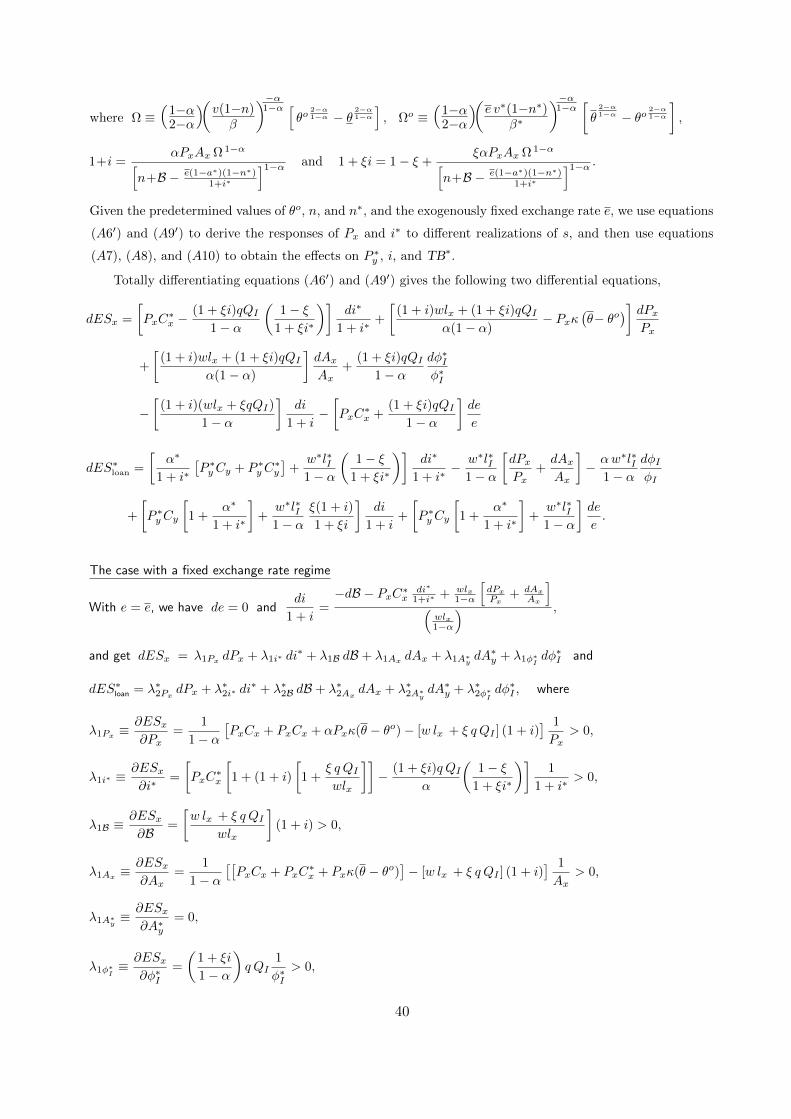
respective partial derivative. Furthermore, it is shown that the responsiveness of the excess supplies
to adjustments in Px and i∗ depends crucially on the fraction of the required upfront payments, ξ.
With outsourcing, θo<θ, we have∂2ESx∂ξ ∂Px
< 0,∂2ES∗loan∂ξ ∂Px
> 0,∂2ESx∂ξ ∂i∗
> 0, and∂2ES∗loan∂ξ ∂i∗
< 0.
An increase in Px lowers the demands Cx and C∗x but increases the supplies Q ihx and Qos
x in the
market for good x, leading to an increase in ESx and liquidity demands wlx and w∗l∗I . The increase
in liquidity demand wlx in the home loan market results in an increase in i, generating negative
effects on the home country’s import Cy and the supplies Q ihx and Q os
x . In the foreign loan market,
the liquidity demand w∗l∗y decreases as Cy decreases, and the liquidity demand w∗l∗I increases as QI
18
increases. As the former effect dominates, there will be a net increase in ES∗loan. With outsourcing,
as only a fraction ξ of the working capital is financed in the home loan market, the negative effects
of an increase in i on Q osx and w∗l∗I will be weak if ξ is small. Hence, the smaller the value of ξ, the
larger the increase in ESx and the smaller the increase in ES∗loan will respond to an increase in Px.
An increase in i∗ reduces the demand C∗x and the supply Q osx in the market for good x. The
first effect would dominate the second effect and result in a net increase in ESx. In the market
for foreign loan, an increase in i∗ leads to decreases in liquidity demands, w∗l∗y and w∗l∗I , causing
an increase in ES∗loan. The smaller the value of ξ, the higher the reliance of the working capital
financing for production of good I is on the foreign loan market, the smaller the increase in ESx
and the larger the increase in ES∗loan will result from an increase in i∗.
Different realizations of the current state s may result in ESx 6= 0 and/or ES∗loan 6= 0. As
shown in Appendix C, with no international outsourcing, there is trade in final goods only, the
equilibrium adjustments of Px and i∗ to different realizations of s depend on the values of a, a∗,
α, and α∗. The parameters a and a∗ measure the degree of home bias in households’ preferences,
determining the strengths of the liquidity flows required for facilitating international final good
trade, PxC∗x and P ∗yCy. The parameters α and α∗ represent the shares of inputs that are subject to
the liquidity constraints, measuring the liquidity needs of the final good producers, wlx and w∗l∗y.
In the case with outsourcing, in addition to final-good trade, there is intermediate-good trade, and
the equilibrium adjustments of Px and i∗ depend on not only the values of a, a∗, α and α∗ but also
the value of ξ. The fraction ξ determines the foreign firms’ reliance on the foreign loan market in
meeting their working capital needs for the production of good I.
Result 1. Under a fixed exchange rate, holding n, n∗ and θo constant, the transmission of the effects
of temporary shocks (different realizations of s) is through not only the channel of final good trade
but also the channel of intermediate good trade. International outsourcing introduces adjustments via
the liquidity demand w∗l∗I and output supply Q osx , while the fraction of upfront contractual payment
ξ determines the strength of these additional adjustments. For a small value of ξ, the presence of
international outsourcing dampens the effects of the home monetary shocks B, and alters qualitatively
the impacts of the home productivity shocks Ax.
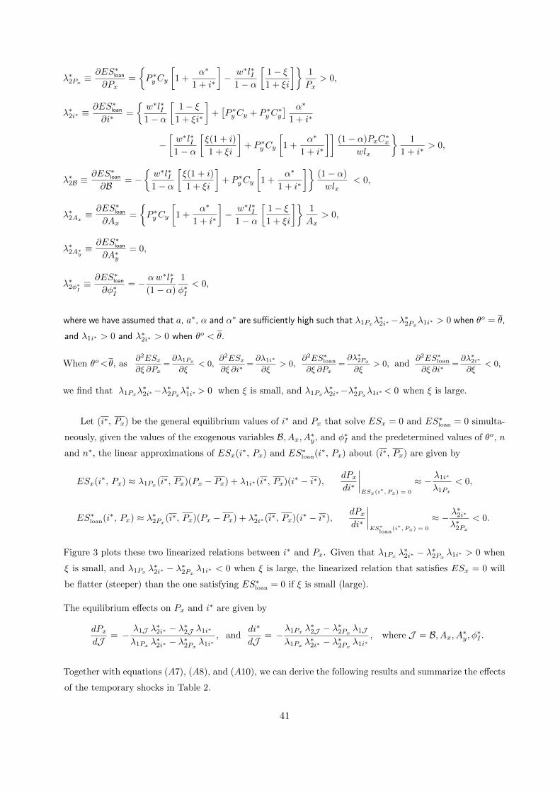
To demonstrate the role of ξ, Figure 3 plots the two linearized relations between Px and i∗
that satisfy respectively equations ESx = 0 and ES∗loan = 0 to present a graphical illustration of
the effects of the monetary and productivity shocks of the home country.25 The two linearized
25As these two excess supply functions are nonlinear, we plot the linearized relations between Px and i∗ using thefirst-order Taylor approximations of ESx = 0 and ES∗loan = 0 around the equilibrium. The derivation is presented inAppendix C. A realization of s determines all the values of B, Ax, A∗y, and φ∗I . To identify the effects, our analysis
19
relations are both negatively sloped; the value of ξ determines their relative slope and the extent
they respond to the shocks. As shown in Appendix C, the linearized relation that satisfies ESx = 0
will be flatter (steeper) than the one satisfying ES∗loan = 0 if ξ is small (large). How ξ affects the
responses of the two relations to the shocks is illustrated below.
Figure 3: The effects of temporary shocks in the home country
The solid lines show the original linearized relations between Px and i∗ around the general equilibrium and
the dotted lines reflect the effects of the shocks on the relations. Under a fixed e regime, the linearized
relation ofES∗loan=0 is steeper than that ofESx=0, except when ξ is sufficiently high.
(a) Monetary shock: an increase in B raises ESx and reduces ES∗loan,
⇒ shifting the ESx = 0 relation downward and the ES∗loan = 0 relation rightward.
fixed e, θo = θ
-
6
0r
Px
i∗
BBBBBBBB
ES∗loan
=0
PPPPPP
ESx=0 q qfixed e, θo< θ, and low ξ
-
6
0r
Px
i∗
AAAAAAAA
ES∗loan
=0
HHHH
HH
ESx=0
qqfixed e, θo< θ, and high ξ
-
6
0r
Px
i∗
AAAAAAAA
ESx=0
HHHH
HHES∗loan
=0
q qflexible e and θo < θ
-
6
0r
Px
i∗
LLLLLLLL
ES∗loan
=0
HHHHHH
ESx=0q q
(b) Productivity shock: an increase in Ax raises both ESx and ES∗loan,
⇒ shifting the ESx = 0 relation downward and the ES∗loan = 0 relation leftward.
fixed e and θo = θ
-
6
0r
Px
i∗
BBBBBBBB
ES∗loan
=0
PPPPPP
ESx=0 qq
fixed e, θo< θ and low ξ
-
6
0r
Px
i∗
AAAAAAAA
ES∗loan
=0
HHHH
HH
ESx=0
qqfixed e, θo< θ, and high ξ
-
6
0r
Px
i∗
AAAAAAAA
ESx=0
HHHHHHES∗
loan=0
q qflexible e and θo< θ
-
6
0r
Px
i∗
AAAAAAAA
ES∗loan
=0
HHHHHH
ESx=0
qq
4.1.a The Effects of a Larger Realization of B
An increase in the open market purchase of home-currency-denominated bonds, B, increases the
liquidity supply in the home loan market and has a downward force on i. Holding Px and i∗
constant, a lower i encourages the supplies Q ihx and Q os
x and the demands Cy and l∗I , resulting in
an excess supply of good x, ESx > 0, and an excess demand for foreign loans, ES∗loan < 0.
In the case with no international outsourcing, θo = θ, i and Px will fall, and i∗ will rise to clear
allows only one of these exogenous shocks to vary at a time. We will discuss the effects of changes in B and Ax, andomit the discussion on A∗y and φ∗I , while their effects are summarized in Table 2.
20
the markets if there is home bias in consumption in each household’s preferences and the liquidity
needs of the final good producers are high (a, a∗, α, and α∗ are sufficiently high). Both the direct
effect of the increase in B and the indirect effects via the decrease in Px and the increase in i∗ have
negative impacts on the home interest rate, i, but positive impacts on the foreign price of good y,
P ∗y , and the foreign trade balance, TB∗.
In the case with international outsourcing, θo < θ, the equilibrium changes in Px and i∗ also
depends on the fraction ξ. When ξ is small, a decrease in Px has a strong negative effects on ESx
and a weak negative effect on ES∗loan; while an increase in i∗ has a weak positive effects on ESx
and a strong positive effect on ES∗loan. Hence, a small decrease in Px and a small increase in i∗
will be sufficient to achieve a new general equilibrium. Similarly, the effects on i, P ∗y , TB∗ will be
qualitatively similar to but quantitatively much smaller than in the case with no outsourcing.26
4.1.b The Effects of a Higher Realization of Ax
If Px and i∗ remain unchanged, a higher realization of Ax will induce the home firms to expand their
production and increase their demands for home-currency-denominated loans, leading to ESx > 0
and an increase i. A higher value of Ax affects the foreign loan market directly by increasing l∗I ,
and indirectly via its upward force on i that leads to decreases in the demands Cy and l∗I . The
decrease in w∗l∗y + P ∗yCy dominates the increase in w∗l∗I and leads to ES∗loan > 0.
With no outsourcing, θo = θ, reaching a new general equilibrium requires only an equal pro-
portional decrease in Px to respond to an increase in Ax, leaving the marginal revenue product
schedules αPxAxθiIiα−1 unchanged. The home firms have no incentive to change their inputs.
There are no effects on the allocation in the liquidity in each loan market and the interest rates i
and i∗. Given that each shopper has a constant expenditure on each good, an increase in Ax and
an equal proportional decrease in Px simply cause Qx, Cx and C∗x to increase proportionally, while
leaving the production and allocation of good y and thus P ∗y , Q∗y, Cy, C∗y , and TB∗ unchanged.
When there is international outsourcing, θo < θ, an equal proportional decrease in Px will
restore ES∗loan = 0, it remains to have ESx > 0 because of the presence of the total real fixed cost
of outsourcing, κ(θ − θo). When ξ is small, the combination of a more than proportional decrease
in Px and an increase in i∗ can help to achieve a general equilibrium. As there is a net decrease in
PxAx, the home firms reduce their liquidity demands and cause the equilibrium value of i to fall.
There will be increases in P ∗y and TB∗ because of the decrease in Px and the increase in i∗.27
26When ξ is large, clearing the markets requires a combination of an increase in Px and a decrease in i∗, while theequilibrium effects on i, P ∗y , and TB∗ will be ambiguous.
27If ξ is large, a combination of a less than proportional decrease in Px and a decrease in i∗ will help achieving thegeneral equilibrium, implying an increase in i and decreases in P ∗y and TB∗.
21
4.1.c The Case with a Flexible Exchange Rate Regime
It would be of interested to investigate whether the dependence of the effects of the monetary and
productivity shocks on the contractual upfront payment arrangement, ξ, would hold under a flexible
exchange rate regime (Z∗ = Z∗ = 0). The derivation of the ESx and ES∗loan equations in the case
with a flexible exchange rate are presented in Appendix C, we have
ESx(Px, i∗, B, Ax, A∗y, φ∗I , θo, n, n∗) and ES∗loan(Px, i
∗, B, Ax, A∗y, φ∗I , θo, n, n∗).
+ + + + 0 + − − + − 0 −
There are two interesting findings. Firstly, the presence of the endogenous adjustment of e alters
the relation of ES∗loan with Px, i∗, and the monetary and productivity shocks qualitatively. Contrary
to the quantity adjustments (official sales of foreign currency, Z∗ and Z∗) in the foreign exchange
market under a fixed e that respond to accommodate the changes in the demand for foreign liquidity,
the price adjustments (relative price of foreign currency, e) in the foreign exchange market under a
flexible e tend to counteract the impacts on the foreign liquidity, resulting in a ES∗loan relation that
is qualitatively different from the one in the case with a fixed e. Secondly, the quantitative and
qualitative differences in the effects of the shocks for different values of ξ do not prevail in the case
of a flexible exchange rate regime. It highlights how the value of ξ determines the strength of the
direct effects of the home country’s shocks on the liquidity allocation in the foreign loan market,
influences the directions and magnitudes of the official intervention required to accommodate the
fixed nominal exchange rate e, and therefore matters for the transmission mechanism.
4.1.d Discussion
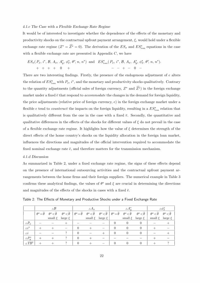
As summarized in Table 2, under a fixed exchange rate regime, the signs of these effects depend
on the presence of international outsourcing activities and the contractual upfront payment ar-
rangements between the home firms and their foreign suppliers. The numerical example in Table 3
confirms these analytical findings, the values of θo and ξ are crucial in determining the directions
and magnitudes of the effects of the shocks in cases with a fixed e.
Table 2: The Effects of Monetary and Productive Shocks under a Fixed Exchange Rate
4B 4Ax 4A∗y 4φ∗I
θo=θ θo<θ θo<θ θo=θ θo<θ θo<θ θo=θ θo<θ θo<θ θo<θ θo<θsmall ξ large ξ small ξ large ξ small ξ large ξ small ξ large ξ
The adjustment at the extensive margin results in a decrease in the liquidity demand in the home
loan market wlx and an increase in the liquidity demand in the foreign loan market w∗l∗I , leading
the households to adjust their deposit decisions in the directions different from those in the case
without outsourcing. In the home loan market, given that the home firms’ liquidity demand w lx
is more sensitive to an increase in e than the foreign importers’ liquidity demand PxC∗x does, there
will be a net decrease in liquidity demand in the home loan market. To eliminate the downward
pressure on i, the home households will reduce their deposits n to satisfy the optimal condition
βE[1 + i] = 1. In the foreign loan market, the increase in liquidity demand for the production of
the intermediate good w∗l∗I dominates the decreases in the liquidity demands for the production
and trade of final good y, P ∗yCy and w∗l∗y. Following the optimal condition β∗E[1 + i∗] = 1, the
foreign households will increase their deposits n∗ to ease the upward pressure on i∗.
The decrease in n implies an increase in the home real wage w; and the increase in n∗ implies
decreases in the foreign real wage, w∗, and price of good I, q∗. Although the increase in e would
raise the home-currency price of good I, e q∗, the relative unit cost of producing to importing good
I, w/(e q∗), increases and induces more home firms to switch to international outsourcing, leading
θo to fall further. The interactions of the adjustment at the extensive margin in outsourcing (the
number of firms sourcing abroad) with the households’ deposit decisions are the driving forces of
the equilibrium effects. It is shown that a revaluation of the foreign currency (an increase in e) has
positive equilibrium effects on n∗ and w/(e q∗), and a negative equilibrium effect on θo.
When θo ∈ ( θ, θ ),dn∗
de> 0,
d (w/(e q∗))
de> 0,
dθo
de< 0,
d (PxC∗x/e)
de< 0, and
dTB∗
de> 0.
Ifd ((1− n)/e)
de< 0, then
dP ∗yCy
de< 0,
d q∗QIde
> 0, andd (q∗QI + P ∗yCy)
de> 0.
A positive effect on n∗ indicates a negative effect on PxC∗x/e. The equilibrium effects on n and
(1−n)/e are ambiguous. If the direct effect of an increase in e dominates, we will get d((1−n)/e)de < 0,
implying a negative effect on P ∗yCy and positive effects on q∗QI and q∗QI+P ∗yCy. Although the net
trade in consumer goods, P ∗yCy − PxC∗x/e, is ambiguous, we show that the foreign trade balance,
TB∗ = q∗QI + P ∗yCy − PxC∗x/e, improves, requiring the foreign monetary authority to conduct
larger official sales of the foreign currency in the foreign exchange market, z∗ ≡ Z∗ + Z∗
1+i∗ rises.
26
Discussions:
The presence of international outsourcing activities is shown to be an important determinant
of the effect of a revaluation on the trade balance TB∗. By looking into the liquidity flows in the
foreign exchange market, we can gain some insights into the interactions at work. The demand
for foreign currency is derived from the home country’s demand for imports of final good y and
intermediate input I, and the supply of foreign currency is derived from the foreign country’s import
of final good x. When θo = θ, there is trade in final goods only, and changes in e induce adjustments
of n and n∗. As P ∗yCy is negatively related to e, and PxC∗x/e is positively related to e, we have the
usual downward sloping demand and upward sloping supply schedules of foreign currency in the
foreign exchange market. An increase in e reduces TB∗, the foreign monetary authority reduces its
official sale of foreign currency Z∗ to meet the decrease in the net private demand.
The incorporation of international outsourcing activities alters the responses of the demand and
supply of foreign currency to changes in e. When θo < θ, with the adjustments of θo, n, and n∗,
an increase in e effectively increases the demand w∗l∗I + P ∗yCy and reduces the supply PxC∗x/e of
foreign currency, resulting in an upward sloping demand and a downward sloping supply schedules
in the foreign exchange market.29 The foreign monetary authority has to conduct larger official
sales Z∗ and Z∗ to meet the increase in the net private demand due to a larger TB∗. As a result,
a revaluation of foreign currency will make the home country’s trade deficit deteriorate further.
This finding provides a rationale for the puzzling evidence of a positive relationship between
China’s currency value and its trade surplus during the period of 1994-2008. Figure 5 presents
the official exchange rate of China’s currency, the Renminbi (RMB), in units of the US dollar and
China’s trade balance in goods and services (TB) as a percentage of its gross domestic product
(GDP) from 1985 to 2016. It also includes the real effective exchange rate (REER) and the decom-
position of the trade balance.30 The correlation coefficient between the official USD/RMB rate and
China’s TB/GDP ratio was −0.72 during the period of 1985-1993 as China’s overall trade balance
tended to improve when RMB was devalued. In contrast, the correlation coefficient was positive
and equal to 0.74 during the period of 1994-2008 and 0.26 for the period of 1994-2016.31 Similar
patterns of the correlation coefficients between the REER the TB/GDP ratio are obtained.
29Recall that w∗l∗I =(1+ξi∗
1+i∗
)q∗QI and TB∗ = q∗QI + P ∗yCy − PxC∗x/e.
30The data are obtained from the World Integrated Trade Solution and the World Development IndicatorsDatabases of the World Bank. The real effective exchange rate is the nominal effective exchange rate (a mea-sure of the value of RMB against a weighted average of several foreign currencies) divided by a price deflator. Dataon the decomposition of the trade balance into the four major product categories (capital goods, consumer goods,intermediate goods, and raw materials) are available from 1992 only.
31The global trade collapse in 2008-2009 and the slow economic recovery may have contributed to this significantdrop in the positive correlation.
27
Figure 5: C
hina’s Exchange R
ates and Net E
xports to GD
P R
atios
60.0
80.0
100.0
120.0
140.0
160.0
-4.00
0.00
4.00
8.00
12.00
All goods T
B/G
DP
Consum
er goods TB
/GD
P
Intermediate goods T
B/G
DP
Real E
ffective Exchange R
ate Index (2010=100)
Adjusted O
fficial US
D/R
MB
Rate (2010=
100)
Exchan
ge R
ates
(20
10
=10
0)
TB/G
DP
(%)
S
ource: The W
orld Develo
pment Indicators and the W
orld Integrated Trade S
olution D
atabases, the World B
ank.
Year
Capital
goods
TB
/GD
P
(%)
Co
nsu
mer
go
od
s
TB
/GD
P
(%)
Interm
ediate
go
od
s
TB
/GD
P
(%)
Raw
Materials
TB
/GD
P
(%)
All
Pro
du
cts
TB
/GD
P
(%)
Real
Effective
Exchange
Rate Index
(RE
ER
)
(2010=100)
Official
Nom
inal
Exchange
Rate,
US
D per
RM
B
1985
-4.97
169.92 0.3405
1986
-4.04
123.72 0.2896
1987
-1.19
107.15 0.2687
1988
-1.91
116.83 0.2687
1989
-1.43
135.20 0.2656
1990
2.19
99.06 0.2091
1991
1.96
87.03 0.1879
1992 -4.65
9.27 -4.11
0.67 1.02
83.52 0.1813
1993 -7.04
9.30 -5.47
0.55 -2.75
88.91 0.1736
1994 -6.07
10.28 -3.51
0.57 0.96
69.68 0.1160
1995 -3.85
8.75 -2.30
-0.17 2.27
77.62 0.1197
1996 -3.06
7.89 -2.92
-0.24 1.41
85.28 0.1203
1997 -1.81
8.86 -2.23
-0.29 4.20
91.82 0.1206
1998 -1.54
8.38 -2.27
-0.17 4.23
96.70 0.1208
1999 -1.90
8.01 -2.66
-0.51 2.67
91.53 0.1208
2000 -1.91
8.47 -2.88
-1.57 1.99
91.48 0.1208
2001 -2.07
7.83 -2.64
-1.35 1.68
95.42 0.1208
2002 -2.06
8.31 -2.82
-1.29 2.07
93.21 0.1208
2003 -2.15
8.89 -3.13
-2.05 1.53
87.11 0.1208
2004 -1.62
9.27 -2.44
-3.53 1.64
84.76 0.1208
2005 0.07
10.26 -1.76
-4.07 4.46
84.25 0.1220
2006 1.02
10.43 -0.51
-4.49 6.45
85.57 0.1254
2007 2.40
9.89 -0.04
-4.80 7.43
88.93 0.1314
2008 3.28
8.27 0.80
-5.81 6.48
97.10 0.1439
2009 2.36
6.65 -0.95
-4.18 3.84
100.40 0.1464
2010 2.57
6.86 -0.74
-5.43 2.98
100.00 0.1477
2011 2.66
6.47 -0.32
-6.14 2.05
102.69 0.1548
2012 2.86
6.45 -0.17
-5.66 2.69
108.44 0.1584
2013 2.68
6.38 -0.07
-5.23 2.70
115.30 0.1614
2014 2.66
6.36 0.06
-4.65 3.65
118.99 0.1628
2015 2.71
5.91 -0.23
-2.96 5.37
131.63 0.1606
2016 2.24
5.21 -0.14
-2.69 4.55
124.26 0.1505
Correlation C
oefficient with R
EE
R
1985-1993
-0.72
1994-2008 0.56
-0.60 0.32
-0.25 0.33
1994-2016 0.73
-0.87 0.67
-0.44 0.28
Correlation C
oefficient with the official U
SD
/RM
B R
ate
1985-1993
-0.72
0.93
1994-2008 0.86
-0.02 0.91
-0.78 0.74
0.44
1994-2016 0.86
-0.80 0.84
-0.73 0.26
0.85
esouser
Typewritten Text
esouser
Typewritten Text
esouser
Typewritten Text
28
After a substantial devaluation of the RMB in 1994, the official USD/RMB exchange rate had
been kept relatively stable, and it remained steady at 12.08 U.S. cents per RMB from 1997 to
2005. The surge of China’s TB/GDP ratio to 4.46% in 2005 ignited the political pressure from
policymakers of other countries, including those of the U.S., on RMB to revalue. China introduced
a new regime in 2005 to allow for graduate revaluations of the RMB. Its trade surplus not only did
not fall but rose substantially to 6.48% of its GDP in 2008 despite of a 20% cumulative appreciation
of the RMB against the US dollar.32 Although many studies in the literature have explained why
the trade flows might not be responsive to the currency revaluations, they could not explain the
accelerating increase in China’s trade surplus. The decomposition of the trade balance reveals that
the net trade flows of different categories of products responded quite differently to the changes in
the currency value. For the period of 1994-2008, the correlation coefficient of the official USD/RMB
rate and the TB/GDP ratio was equal to 0.91 for the intermediate goods and−0.02 for the consumer
goods, while for the period of 1994-2016, they were equal to 0.84 and −0.80, respectively. These
correlations are in line with our model predictions that a revaluation of the foreign currency would
increase the foreign country’s exports of intermediate goods, while having an ambiguous effect on
its trade balance of the consumer goods.
The increases in the differences in the labor costs of China and the U.S. are consistent with
the increases in China’s outsourcing activities and exports of intermediate goods. According to the
Bureau of Labor Statistics of the United States Department of Labor, the hourly labor compensation
in China’s manufacturing sector increased from USD0.60 in 2002 to USD1.74 in 2009, while those
of the U.S. increased from USD27.36 to USD34.19. Although the hourly labor compensation in
China increased from about 2% of the U.S. level in 2002 to 5% in 2009, the level differences were
widened and the labor cost in China remained very low.33
Our model provides a theoretical framework to illustrate how the rise of China as a major host
country of international outsourcing may have altered the response of the overall trade balance to
its currency revaluation, helping to rationalize the relation between its currency revaluation and
trade surplus.
32Although its trade flows and trade surplus have been declining since global trade collapsed in 2008, China hasbecome the world’s largest exporter since 2009. According to the World Trade Report 2013, its share of world exportwas 11% in 2011. The upward trend in the trade balance has been observed in the recent years.
33The hourly labor costs in China and the U.S. are from the website of the Bureau of Labor Statistics of theUnited States Department of Labor, http://www.bls.gov/fls/home.htm, which provides data from 2002 to 2009 only.Some reasons for the increases in China’s labor costs were rising labor productivity, inflation, and the increasedrequirements for social insurance payments by firms.
29
4.2.b Effects of Reductions in the Costs Associated with International Outsourcing
We now consider the effects of a reduction in the fixed cost of international outsourcing κ. In order
to disentangle the direct effects of a reduction in κ and the indirect effects of the induced official
interventions under a fixed nominal exchange rate regime, our analysis will proceed in two steps.
Firstly, we investigate the effects on the households’ decisions and the nominal exchange rate by
assuming that z∗ is held constant and e is allowed to adjust endogenously to clear the foreign
exchange market. Secondly, maintaining the nominal exchange rate at e requires the foreign mon-
etary authority to conduct official sales/purchases of its currency in the foreign exchange market,
we identify the required endogenous adjustment of z∗ and the effects on the world economy. We
can then combine the effects to obtain the equilibrium impacts of an increase in κ under a fixed
exchange rate regime and have a better understanding of the driving forces behind the findings.
Result 3. A reduction in the fixed cost of international outsourcing encourages more home firms to
switch to sourcing abroad under a flexible exchange rate, while the endogenous adjustment in the official
sale of foreign currency for maintaining a fixed exchange rate will discourage outsourcing.
Holding z∗ constant, a reduction in κ encourages some home firms to switch from producing
their intermediate inputs domestically to importing from aboard, resulting in a fall in θo, a decrease
in liquidity demand w lx in the home loan market, and an increase in the liquidity demand w∗l∗I in
the foreign loan market. In the foreign exchange market, the increase in the home country’s demand
for foreign currency q∗QI generates an upward force on e, it will discourage the foreign country’s
export of good y, P ∗yCy, but leave the home country’s export of good x, PxC∗x/e, unchanged if
n and n∗ do not adjust. In the foreign loan market, a decrease in P ∗yCy also reduce the liquidity
demand w∗l∗y, leading the foreign households to reduce their deposits n∗ until the optimal condition
β∗E[1 + i∗] = 1 is satisfied. In the home loan market, if the decrease in wlx is dominated by the
increase in PxC∗x, there will be a net increase in liquidity demand, and the home households will
increase their deposits n until the optimal condition βE[1 + i] = 1 is met. It can be shown that
de
dκ
∣∣∣∣dz∗=0
< 0,dθo
dκ
∣∣∣∣dz∗=0
> 0,d((1− n)/e
)dκ
∣∣∣∣∣dz∗=0
> 0, anddn∗
dκ
∣∣∣∣dz∗=0
> 0.
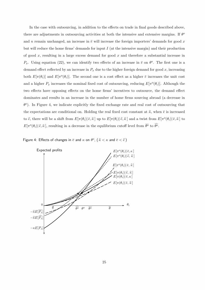
As shown in Figure 4, a reduction from κ to κ, while letting e adjust freely, causes the equilibrium
exchange rate to increase from e to e and cutoff productivity level to decrease from θo to θo ,
encouraging more home firms to outsource abroad.
Keeping the exchange rate at e in face of a lower κ is like conducting a devaluation of the foreign
currency to bring the exchange rate from the new market equilibrium level e down to its original
30
fixed level e, requiring the a reduction in the foreign official sale of foreign currency z∗. As discussed
in Section 4.2.a, a reduction in e has a positive effect on θo and a negative effect on TB∗. As the
direct effect from a lower κ and the indirect effect from a lower z∗ affect θo in opposing directions,
the equilibrium effect is ambiguous. Figure 4 illustrates how keeping the nominal exchange rate at
e means further shifts in the expected profits schedules which may result in a new equilibrium level
at θo, having a net increase in the cutoff level, θo < θo < θo. The numerical example presented in
Table 4 shows that the indirect effect could dominate and result in an increase in θo.
5 Welfare Analysis
The equilibrium effects of the exogenous changes on the welfare of each household are generally
ambiguous as the direct and indirect effects are in opposing directions. Tables 3 and 4 construct
some numerical examples to illustrate the welfare impacts of various exogenous changes. It should
be noted that the equilibrium welfare effects depend on the specifications of the utility functions,
and that the aim of these exercises is to illustrate the theoretical properties of the model rather
than to match the observed data.
5.1 Welfare Effects of Different Realizations of s
Given e and κ, holding θo, n, and n∗ constant, we can use our findings of changes in i, i∗, Px, and
P ∗y to determine the impacts on households’ consumption and leisure levels and pin down the welfare
effects of different realizations of s. The results of the numerical exercises are presented in Table 3.
First, the presence of international outsourcing weakens the welfare effects of domestic mon-
etary policy on the world economy. An increase in the open market purchase of home-currency-
denominated bonds B reduces Px and i but increases P ∗y and i∗, leading to increases in Cx, Cy,
and h but decreases in C∗x, C∗y , and h∗. Because of home bias in consumption, households expe-
rience substantial welfare gains (losses) from the increases (decreases) in the consumption of the
domestically produced final good when its price falls (rises). In addition, a decrease (an increase)
in the domestic interest rate lowers (raises) the domestic-currency price of the imported final good,
leading to an increase (a decrease) in the consumption of the imported final good. As the welfare
changes from the adjustments in consumption dominate the impacts from the adjustments in work
effort, u increases and u∗ decreases. The smaller the value of ξ, the less responsive the adjustments
in Px, i, P ∗y and i∗, and the weaker the equilibrium effects on u and u∗ will be.
Second, no matter whether there are international outsourcing activities, an improvement in
31
the production technology of a final good (an increase in Ax or A∗y) benefits the households of both
countries. The increases in consumption of the final good that experiences a positive productivity
shock play dominant roles in improving the welfare levels of the households.34
5.2 Welfare Effects of Changes in e or κ
The adjustments of θo, n, and n∗ in response to the changes in e or κ determine the allocation
of liquidity in the world economy. As shown in Table 4, given that transactions are facilitated by
liquidity, the adjustments of deposit decisions n and n∗ are good indicators of the welfare effects.35
Table 4 : Numerical Exercises of Permanent Changes in e and κ for Sections 4.1 and 5.1a
Case I: θo = θ Case II Case III
κ is prohibitively high Outsourcing with κ = 0.2, θo < θ Outsourcing with κ = 0.1, θo < θ
a These numerical exercises assume no uncertainty. The parameter values are β = β∗ = 0.96, a = a∗ = 0.6, α = α∗ = 23
,
v = 1, v∗ = 0.9, B = 0, Ax = A∗y = 4, φ∗I = 1, θ = 0, θ = 1, and ξ = 0.3. In the cases with θo = θ, there is nointernational outsourcing as the value of κ is prohibitively high.
b The equilibrium under this fixed exchange rate e is also the equilibrium under a flexible exchange rate regime.
c If e = 1 and κ is prohibitively high originally, these are examples of fixed exchange rate levels that will benefit bothcountries when κ becomes lower.
d Comparing to the equilibrium with κ = 0.2 and e = 1.07, this fixed exchange rate level can make both countriesbetter off when κ falls to equal to 0.1.
5.2.a Welfare Effects of an Increase in e
As shown respectively in Cases II and III of Table 4, holding κ constant, an increase in e leads
some home firms to switch to international sourcing (θo falls); and the reallocations of liquidity in
34When ξ is small, an increase in φ∗I reduces Px and i but increases P ∗y and i∗, leading to increases in Cx, Cy, andh but decreases in C∗x , C∗y , and h∗, resulting an increase in u and a decrease in u∗.
35The numerical example assumes ξ = 0.3. However, the qualitative effects on the welfare levels of an increase ine or a reduction in κ are not sensitive to the value of ξ.
32
the loan markets induce a decrease in n and an increase in n∗. A decrease in n implies that higher
consumption expenditures are available for the home shoppers while fewer loans are available for
the hiring of workers in the home country, Cx and Cy increase and h falls. An increase in n∗
indicates that the foreign shoppers’ consumption expenditures are lower and that the foreign firms
obtain more loans to hire workers in the foreign country, C∗x and C∗y decrease and h∗ rises. Hence,
a revaluation of the foreign currency leads to an increase in u and a decrease in u∗. It is found that
u is increasing and u∗ is decreasing in e, and the total utility level of the two counties, u+ u∗, can
be increasing in e when the utility function is linear in leisure.36 In contrast, with no outsourcing,
a foreign currency revaluation increases n and reduces n∗, improving the welfare of the foreign
households, while making the home households worse off. Case I of Table 4 illustrates that when
θo = θ, u is decreasing and u∗ is increasing in e, and the total utility u+ u∗ displays an inverted U
relationship as e increases, reaching its maximum at the flexible exchange rate equilibrium. These
results highlight the important role of international outsourcing in the determination of the welfare
effects of currency revaluations on the world economy.
5.2.b Welfare Effects of a Reduction in κ
A reduction in the fixed cost of outsourcing improves the welfare of the foreign households but
makes the home households worse off under a flexible exchange rate regime. As the comparison of
columns I.2, II.1, and III.2 in Table 4 illustrates, when the exchange rate is flexible (z∗ = 0), a
decrease in κ increases e and n but reduces θo and n∗. The changes in households’ consumption
expenditures result in decreases in Cx and Cy and increases in C∗x and C∗y . Although h falls and
h∗ rises when more production activities are relocated to the foreign country, the welfare changes
from the adjustments in consumption dominate, leading to a decrease in u and an increase in u∗
and resulting in a small net increase in the total utility level u+ u∗.
The presence of a fixed exchange rate regime reinforces the welfare effects. The foreign exchange
intervention that prevents the exchange rate from increasing and keeps it at the level e works like
a policy to devalue the foreign currency, reducing the home country’s welfare and improving the
foreign country’s welfare further. Consider the original equilibrium given by column II.1. Under a
36It is noted that the increase in u+u∗ cannot go unbounded as the foreign labor effort, h∗, will reach its upper boundeventually. When there is diminishing marginal utility of leisure, the total utility level of the two counties, u + u∗,may not be monotonic in e. For example, in the case with u(Cx, Cy, h) = a lnCx + (1− a) lnCy + 1