International Trade and Income Inequality * Taiji Furusawa † University of Tokyo Hideo Konishi ‡ Boston College Tran Lam Anh Duong § University of Tsukuba September 22, 2018 Abstract We propose a simple theory that shows a mechanism through which international trade entails wage and job polarization. We consider two countries in which individuals with different abilities work either as knowledge workers, who develop differentiated products, or as production workers, who engage in production. In equilibrium, ex ante symmetric firms attract knowledge workers with different abilities, which create firm heterogeneity in product quality. Market integration disproportionately benefits firms that produce high-quality products. This winner-take-all trend of product markets causes war for talents, which exacerbates income inequality within the countries and leads to labor-market polarization. JEL classification numbers: F12, F16, J31. Keywords: Job polarization, middle-income class, globalization, income inequality, firm heterogeneity. * We are grateful to participants of Asia Pacific Trade Seminars (APTS) 2012, Asian Meeting of the Econo- metric Society (2013), the 2012 Association for Public Economic Theory Meeting in Taipei, Australasian Trade Workshop (2013), Hitotsubashi GCOE Conference on International Trade and FDI 2012, the 2012 annual meeting of the Japan Society of International Economics, Midwest International Group Meeting (fall 2012), and Villars Workshop 2013, and the seminars at various universities, and James Anderson, Pol Antr` as, Arnaud Costinot, Elhanan Helpman, Oleg Itskhoki, Tomoya Mori, Peter Neary, Gianmarco Otta- viano, Esteban Rossi-Hansberg, Thomas Sampson, and Anthony Venables for helpful comments. We also thank Laura Bonacorsi and Mina Taniguchi for their research assistance. Part of this research was conducted when Furusawa visited Harvard University and the CES. Furusawa gratefully acknowledges their hospitality and financial support of the Abe Fellowship and the CES. We are grateful to anonymous referees for their helpful comments. † Graduate School of Economics, University of Tokyo. Email: [email protected]‡ Department of Economics, Boston College. Email: [email protected]§ Faculty of Engineering, Information and Systems, University of Tsukuba. Email: an- [email protected]
Transcript
International Trade and Income Inequality∗
Taiji Furusawa†
University of Tokyo
Hideo Konishi‡
Boston College
Tran Lam Anh Duong§
University of Tsukuba
September 22, 2018
Abstract
We propose a simple theory that shows a mechanism through which international tradeentails wage and job polarization. We consider two countries in which individualswith different abilities work either as knowledge workers, who develop differentiatedproducts, or as production workers, who engage in production. In equilibrium, ex antesymmetric firms attract knowledge workers with different abilities, which create firmheterogeneity in product quality. Market integration disproportionately benefits firmsthat produce high-quality products. This winner-take-all trend of product marketscauses war for talents, which exacerbates income inequality within the countries andleads to labor-market polarization.
∗We are grateful to participants of Asia Pacific Trade Seminars (APTS) 2012, Asian Meeting of the Econo-metric Society (2013), the 2012 Association for Public Economic Theory Meeting in Taipei, AustralasianTrade Workshop (2013), Hitotsubashi GCOE Conference on International Trade and FDI 2012, the 2012annual meeting of the Japan Society of International Economics, Midwest International Group Meeting(fall 2012), and Villars Workshop 2013, and the seminars at various universities, and James Anderson, PolAntras, Arnaud Costinot, Elhanan Helpman, Oleg Itskhoki, Tomoya Mori, Peter Neary, Gianmarco Otta-viano, Esteban Rossi-Hansberg, Thomas Sampson, and Anthony Venables for helpful comments. We alsothank Laura Bonacorsi and Mina Taniguchi for their research assistance. Part of this research was conductedwhen Furusawa visited Harvard University and the CES. Furusawa gratefully acknowledges their hospitalityand financial support of the Abe Fellowship and the CES. We are grateful to anonymous referees for theirhelpful comments.†Graduate School of Economics, University of Tokyo. Email: [email protected]‡Department of Economics, Boston College. Email: [email protected]§Faculty of Engineering, Information and Systems, University of Tsukuba. Email: an-
ing, as well as importing, can cause income inequality. Bernard and Jensen (1997) find that
1
the wage gap between non-production and production workers increased in the 1980s and
that exporting plants contribute heavily to this change. Baumgarten (2013) and Danziger
(2017) also document that the wage premium in exporting establishments is higher than
domestic ones. As for the impact of globalization in general, Autor and Dorn (2013), Goos
et al. (2009, 2014), and Michaels et al. (2014) find that openness to trade and offshoring
have contributed to income inequality, albeit less so than the routine-biased technological
change.
International trade in goods has a large impact on industries and in turn on the labor
market.1 This study proposes a simple theory to show that growing international trade
in goods exacerbates within-country income inequality and can cause job polarization; the
model can explain in particular that the real incomes for the top income earners and the
lowest income earners rise while those for the middle-income class decline.2
Thanks to the ICT (information and communication technology) revolution, it has be-
come much easier for consumers to access detailed product information and to make com-
parisons between similar products. As a result even a small difference in product quality can
lead to a large differential in firms’ profitability within industries: firms that sell high-quality
products command disproportionately high market shares. But this winner-take-all trend
of product markets causes war for talents, since what determines the product quality is the
talents of knowledge workers, such as managers and R&D workers. Consequently, knowledge
workers in winning firms earn disproportionately high income as a rent for their talents. A
greater opportunity of international trade amplifies this effect. A decrease in trade costs
(including marketing and other costs in foreign countries), also caused mostly by the ICT
revolution, has increased the volume of world trade. The proliferation of international trade
1Autor et al. (2013) estimate that import competition from China explains 1/4 of the contemporaneousaggregate decline in US manufacturing employment. Burstein and Vogel (2010) estimate that globalization(i.e., trade in goods and multinational production) accounts for 1/9 of the 24% rise in the US skill premiumbetween 1966 and 2006.
2A growing share of the middle-income class serves as an engine of economic growth. This class also playsan important role in political stability (Acemoglu and Robinson, 2006). So a decline in the middle-incomeclass may have serious economic and political consequences. Autor, et al. (2017) also find evidence that inthe United States, growing exposure to Chinese import competition engendered political polarization, suchthat districts subject to greater import competition became less likely to elect a moderate Democrat andmore likely to elect a conservative Republican, leaving few centrists in either party.
2
naturally widens profit differentials among firms within industries and hence widens income
inequality between and within different skill groups.
To show this phenomenon, we build a two-country variant of Lucas’s (1978) model in
which ex ante symmetric firms in a representative differentiated-good (manufacturing) sector
hire knowledge workers with different abilities, thereby producing products with different
qualities. Firms also hire production workers to produce their products. We assume that
workers are homogeneous in their productivities when hired as production workers despite
the difference in their abilities. In equilibrium, knowledge workers are sorted into different
firms according to their abilities; firms that hire a group of highly-talented knowledge workers
produce high-quality products, while those that hire mediocre knowledge workers produce
low-quality products. The wage gap may arise between knowledge workers and production
workers within a firm, which is particularly serious for profitable firms that produce high-
quality products.
International trade affects firms’ profitability differently. Top-tier firms that produce
high-quality products are the winners of globalization; getting access to additional markets
gives them large benefits. The medium-tier and lowest-tier firms, on the other hand, lose
from globalization. They suffer from foreign top-tier firms’ penetration into their own market.
Although the medium-tier firms may sell their products to foreign markets as well as their
own, additional export profits after the subtraction of fixed costs of export are not enough
to offset the loss that they incur in their domestic market. The lowest-tier firms are forced
to exit due to the intensified competition in the domestic market. Consequently, top income
earners who are the most talented and work for the top-tier exporting firms benefit from
opening to trade; they are the winners of globalization. On the contrary, workers in the
middle-income class, who work as knowledge workers in the middle-tier and lowest-tier firms,
are likely to suffer from opening to trade. Their incomes fall because the profits for the firms
in which they are working fall after trade liberalization. Some workers with intermediate
abilities may also drop from the pool of knowledge workers to the pool of production workers,
thereby receiving lower wages, as the weakest firms exit from the market. Although the real
3
wages for the middle-income class may still rise thanks to the increased varieties of products
available for consumption after trade liberalization, we show that under a relatively mild
condition their real wages unambiguously decline by opening to trade. Indeed, workers in
the middle-income class are the only losers from trade liberalization. The real wages for the
least talented workers, who work as production workers, increase when the country opens to
trade, thanks to the increased varieties of consumption.
As a corollary to this theoretical consequence of globalization, we obtain a testable pre-
diction that the wage gap between knowledge and production workers expands within the
top-tier firms while it shrinks within others. Verhoogen (2008) finds evidence that is consis-
tent with this prediction. He documents that exchange rate devaluation during the peso crisis
of 1993-1997 induced more productive Mexican plants to increase exports and raise wages,
especially for white-collar wages. In this phase, within-firm wage difference between white-
collar and blue-collar workers widens for more productive firms, suggesting that exporting
induces firms to upgrade product quality and reward white-collar workers disproportion-
ately. Friedrich (2015) also finds evidence from Danish data that trade induces exporting
firms to increase sales, add more layers of hierarchy, and increase wage inequality within
those firms. He also documents that even when controlling for the number of hierarchical
layers, an increase in sales leads to a widening of within-firm wage inequality.
After presenting our main results of the paper in the baseline model with two symmetric
countries, we also extend the model in Section 5 to the case where countries are asymmetric
in the population size and ability distribution. We find through numerical simulations that
international trade exacerbates income inequality within the countries. Income inequality in
the trade equilibrium is greater in the smaller country in the case of population asymmetry,
while it is greater in the talent-abundant country in the case of ability-distribution asym-
metry. In the online appendix, we conduct a simple empirical analysis and find from the
data for the OECD countries in the period of 1979-2014 that, based on column (4) in the
appendix table (which includes both country and year fixed effect), trade increases income
inequality but less so in larger countries, as predicted by the model. However, these effects
4
are not statistically significant.3
We are certainly not the first to theoretically predict that international trade widens
wage gap across different income groups. Blanchard and Willmann (2016), Costinot and
Vogel (2010), Helpman et al. (2010a,b), Helpman et al. (2016), Manasse and Turrini (2001),
Sampson (2014), and Yeaple (2005) among others show in their respective models that inter-
national trade in goods widens wage gap within countries.4 Among these studies, Manasse
and Turrini (2001) and Yeaple (2005) are the closest to our paper.
Manasse and Turrini (2001) employ the same basic model structure as ours; ex ante
symmetric firms produce products of different qualities because they are run by entrepreneurs
with different skills. They show, among other things, that skill earnings in non-exporting
firms are reduced relative to those in exporting firms as a result of further trade integration.
In their analysis, however, the mass of entrepreneurs (i.e., workers with skills), which is equal
to the mass of firms in the differentiated-good industry by construction, is fixed and it is not
affected by opening to trade. As a consequence, they cannot analyze how trade liberalization
affects individual worker’s occupational choice when trade induces weak firms to exit from
the market. This channel is important when we assess the impact of trade liberalization
on wage distribution within countries, because the winner-take-all trend in product markets
is reinforced by globalization, thereby reducing the number of firms in each industry and
reducing knowledge workers’ jobs in the middle-income class. In addition, their model does
not show that international trade adversely affects the middle-income class.
Yeaple (2005) derives similar predictions to ours in a similar model environment. In his
model, firms choose both their individual production technologies and the types of workers.
A distinguishing feature of his model is the complementarity between the technology and
skills of labor; high-productivity technology is matched with high-skilled workers. Among
other things, he shows that a reduction in trade costs may decrease the real wage of mod-
erately skilled workers. Beside the fact that the endogenously-determined average talent of
3To the best of our knowledge, there is no paper that empirically examines how the effect of tradeliberalization on income inequality is related to the country size.
4See Grossman (2013) for a thought-provoking survey on the impact of international trade on labormarkets.
5
knowledge workers is the only source of firm heterogeneity in our model, our model is differ-
ent from his in the important aspect that we separate labor into two endogenously allocated
categories: knowledge workers and production workers. This distinction is a key to our
analysis. First, we can discuss the differential effects of trade on workers within firms, which
is another important wage gap besides the wage gap within sectors and within occupations.
Second, we can show that under the mild condition (on the elasticity of substitution) the
real incomes unambiguously fall as a result of globalization for some workers in the middle-
income class because they drop out of the pool of knowledge workers and work as production
workers after trade is liberalized. Third, and more broadly, separating knowledge workers
from production workers is critical in understanding the effect of globalization on the la-
bor market. Knowledge can be embedded into products so that it is duplicated limitlessly
with the help of capital and production workers, allowing firms to possibly earn a fortune
in the global market. Globalization does not necessarily increase the demand for knowledge
workers. (Indeed, our model predicts that demand decreases as a result of globalization.) It
only increases the demand for talent. Knowledge created by a limited number of knowledge
workers is embedded in the products and travels all over the world.
Monte (2011) and Egger and Kreickemeier (2012) also extend Lucas’s (1978) model to
examine the impact of international trade on income distribution. Since their interest is
slightly different from ours, they do not show that trade reduces the real wage of the middle-
income class.
We believe that our model is the simplest one to show the adverse effect of trade on
the middle-income class, while capturing the important aspects of globalization: the winner-
take-all market and war for talents. Our model, which incorporates workers’ occupational
choice, can show that international trade entails labor market polarization that involves the
occupational shift from a knowledge-worker job to a production job. It can also show that
trade increases within-firm wage gaps in large exporting firms while it decreases wage gaps
in smaller firms. In addition, the model is extended to the case of asymmetric countries to
show numerically that trade exacerbates income inequality, particularly in small countries.
6
2 The Model
We consider a model with two countries (countries 1 and 2), one good (a differentiated good
with many varieties), and one production factor (labor). The differentiated good consists
of a continuum of varieties, each of which (denoted by ω ∈ Ω) is produced by a firm under
monopolistic competition. Product quality, which is represented by α(ω), may differ across
varieties. Following Manasse and Turrini (2001) and Caliendo and Rossi-Hansberg (2012),
we represent a representative consumer’s preferences by the utility function:
u =
[∫Ω
α(ω)1σx(ω)
σ−1σ dω
] σσ−1
, (1)
where x(ω) denotes the consumption level of a variety ω and σ > 1 denotes the elasticity
of substitution. The higher the α(ω), the higher the utility a consumer derives from the
consumption of variety ω.
In each country i = 1, 2, there is a continuum of workers with the mass Li; each worker
provides 1 unit of labor. Labor is the only production factor in this economy. But a worker
is employed either as a knowledge worker to develop a product or as a production worker
to produce the good. We choose labor provided by production workers as the numeraire.
Workers are heterogeneous in their abilities, which only matter when they are hired as
knowledge workers. Thus, they are heterogeneous as knowledge workers, but homogenous
as production workers. In the baseline model, ability is measured by a ≥ a0 (where a0 > 0
is the lowest ability), the distribution of which in country i is represented by the cumulative
distribution function Gi with the probability density function gi. The mass of workers with
their abilities less than or equal to a is, therefore, given by LiGi(a). In the baseline model,
we assume that countries 1 and 2 are symmetric: that is, L1 = L2 = L and G1(a) = G2(a) =
G(a) for all a ≥ a0.
The goods market is under monopolistic competition with free entry and exit. To enter,
firms need to develop a product by hiring l knowledge workers, which serves as an entry
cost. The average ability of these workers determines the quality of the product; we simply
assume that the quality of the product α(ω) is equal to the average ability of the knowledge
7
workers employed in the firm. Production itself requires only production workers; 1 unit of
labor produces 1 unit of the good.
There is no friction in the labor markets for either knowledge workers or production
workers, nor does there exist any information asymmetry between workers and firms about
individual workers’ abilities. Since the average ability of knowledge workers determines the
product quality, firms in the differentiated good sector compete for talent. They post wages
for knowledge workers, and workers apply for those positions; we assume that each firm
offers a wage that is common to every knowledge worker within the firm, regardless of the
workers’ abilities.5 Then, each firm chooses l workers from those who have applied.
In equilibrium, matching between firms and knowledge workers must be stable. As a
consequence of the competition among firms, the entire operating profits for each firm are
given as a rent to the knowledge workers. Therefore, given that the average ability of
knowledge workers determines the product quality and that they receive the same wage
within the firms, they have a strong incentive to be matched with other knowledge workers
with abilities that are greater than or equal to their own. As a result, knowledge workers
are sorted into the firms according to their abilities. Since the most talented workers are
in limited supply, the firms post different wages for knowledge workers, attracting workers
with different abilities. Workers are sorted according to their abilities such that workers with
the highest abilities are hired by the firms that post highest wages. Then, it follows from
the assumption of a continuum of workers that all knowledge workers in a firm will have a
common ability. Letting w(ω) denote the knowledge workers’ wage (or rent) in the firm that
produces the variety ω and π(ω) denote the firm’s operating profits, we therefore have
w(ω)l = π(ω). (2)
Firms produce varieties of different qualities in equilibrium. The exogenously-given abil-
ity distribution determines the firm distribution with respect to their product quality, since
5We will show that in equilibrium, the abilities of knowledge workers are the same within the firms. If weassume, alternatively, that a firm posts a wage profile that possibly assigns a higher wage to a worker witha higher ability, we would have another equilibrium in which a firm attracts workers with different abilities.But such equilibrium would disappear if (even a slight) complementarity between knowledge workers isintroduced. We make this assumption of common wage to avoid unnecessary complications.
8
workers are sorted according to their abilities and the average ability of knowledge workers
determines the product quality. The distribution of workers with respect to their abilities is
characterized by a density function of Lg(a). Since all knowledge workers in a firm will have
a common ability, the density of firms that produce varieties of quality α, which is denoted
by f(α), is given by
f(α) =Lg(α)
l. (3)
Workers who are not hired as knowledge workers will work as production workers. In
equilibrium, there will be a cutoff ability α∗ such that all workers with a ≥ α∗ work as
knowledge workers, while all workers with a < α∗ work as production workers. Once α∗ is
given, together with (3), the product quality distribution of operating firms is completely
determined.
3 Autarkic Equilibrium
This section derives the autarkic equilibrium and shows that knowledge workers receive
higher wages than production workers and that their wages increase proportionately with
their abilities. Thanks to the symmetry assumed in the baseline model, we need only consider
a representative country to derive the autarkic equilibrium.
First, we use a consumer’s (or worker’s) demands derived from (1) to obtain a firm’s
production level and profits. Since the wage rate of production workers is normalized to 1,
each firm optimally selects the price p(α) = σ/(σ − 1), the constant mark-up price over the
marginal cost of 1, regardless of its product quality α. Consequently, the firm that produces
a variety of quality α sells
x(α) =αp(α)−σ∫∞
α∗ α′p(α′)1−σf(α′)dα′I =
α∫∞α∗ α′f(α′)dα′
(σ − 1)I
σ(4)
units of the good, where I denotes the aggregate income of the country. The higher the
quality of its product or the smaller the quality index (denoted by∫∞α∗ α
′f(α′)dα′), the
higher the production level of the firm. The operating profits for the firm that produces a
9
product with quality α are given by
π(α) =αI
σ∫∞α∗ α′f(α′)dα′
. (5)
Henceforth, we identify a firm by the quality of its product rather than ω ∈ Ω, since all firms
that produce a good of the same quality have common characteristics.
Let w(α) denote the wage for a knowledge worker with ability a = α, who is hired by
the firm that produces the product of quality α (with a slight abuse of notation). We can
write the profits for the firm as
π(α) = π(α)− w(α)l.
If π(α) is strictly positive for some firm with α, an entrant would post a slightly higher
wage than w(α) and get all the knowledge workers from that firm and operate profitably.
Therefore, π(α) = 0 in equilibrium, so that the knowledge workers’ wage schedule is given
by w(α) = π(α)/l, as (2) indicates.
The equilibrium is characterized by the two conditions: the free-entry (FE) condition
and the labor-market clearing (LM) condition. The free-entry condition expresses that the
operating profits for the cutoff firms with α∗ are just large enough for them to pay the wage
of 1 to each knowledge worker.6 The knowledge workers in the cutoff firms earn the wage
of 1, i.e., w(α∗) = 1, since if w(α∗) > 1 profitable entry by a firm that attracts knowledge
workers with an ability slightly lower than α∗ at the wage [w(α∗) + 1]/2, for example, would
arise. Thus, the free-entry condition can be written as
α∗I
σ∫∞α∗ αf(α)dα
= l. (6)
The labor-market clearing condition, on the other hand, expresses that total labor demands,
the sum of demands for knowledge workers and those for production workers, must equal
the labor supply L. Total demands for knowledge workers are given by l∫∞α∗ f(α)dα. Total
demands for production workers equal (σ − 1)I/σ as we can easily obtain from (4). Thus,
6Note that α∗ denotes both threshold ability for knowledge workers and the quality of the cutoff firms’products, since these firms that produce products of quality α∗ hire knowledge workers with ability α∗.
10
the labor-market clearing condition can be written as
l
∫ ∞α∗
f(α)dα +σ − 1
σI = L. (7)
Figure 1 depicts the relationships between α∗ and I that express the free-entry and labor-
market clearing conditions. The free-entry condition is expressed by a negatively-sloped
schedule FE, since the left-hand side of (6) increases with both α∗ and I. The labor-market
clearing condition, on the other hand, is expressed by a positively-sloped schedule LM , since
the left-hand side of (7) decreases with α∗ but increases with I. The intersection of these
two schedules gives us the autarkic equilibrium values of α∗ and I, which we call α∗A and IA.
Once the equilibrium threshold α∗A is determined, the equilibrium wage schedule is readily
obtained. As Figure 2 shows, wages are flat at 1 for all workers with abilities smaller than
α∗A. Their wages are 1 because they work as production workers. Those who have abilities
greater than α∗A, on the other hand, work as knowledge workers. Their wages are the rents
for their abilities and are greater than 1, except for those whose ability levels are exactly
equal to α∗A. As we can see from (5), the ratio of wages for knowledge workers with any two
different levels of abilities is equal to the ratio of their abilities itself:
wA(α)
wA(α∗A)=
π(α)
π(α∗A)=
α
α∗A,
where we can compare the wage for a knowledge worker with ability a = α with that for
a knowledge worker with ability a = α∗A. It follows from wA(α∗A) = 1 that we can write a
worker’s wage as a function of her ability:
wA(a) =
1 if a0 ≤ a < α∗A
a/α∗A if a ≥ α∗A.
We can view this result from the perspective of wage gaps within firms to obtain the following
proposition.
Proposition 1 The higher the quality of a firm’s product and hence the larger the firm’s
size, the larger the wage gap between knowledge workers and production workers within the
firm.
11
The equilibrium utility for a worker, which can also be considered her real wage, can
be readily derived. It is easy to infer from (4) that the worker with ability a consumes
α(σ−1)wA(a)/σ∫∞α∗Aα′f(α′)dα′ units of each variety of quality α ≥ α∗A. Then it follows from
(1) that the worker’s indirect utility in the autarkic equilibrium is given by
uA(a) =(σ − 1)wA(a)
σ[∫∞
α∗Aαf(α)dα
] 11−σ
. (8)
Not surprisingly, the equilibrium utility for an individual depends on both her wage and the
quality index of the market.
4 Trade Equilibrium
Let us turn to the analysis of the impact of international trade on the firms’ activities and
the wage schedule in the individual countries. We suppose that firms incur fX units of labor
as the fixed cost of exporting. Exporting firms also incur iceberg trade cost such that they
need to ship τ(> 1) units of the good to supply 1 unit in the foreign market.
We consider a realistic case in which only a fraction of the firms export their products.
Let αX denote the threshold quality such that the products are exported (as well as supplied
domestically) if and only if their individual product qualities are higher than or equal to αX .
It is easy to see that the operating profits from the domestic and foreign sales are given by
πd(α) =αI
σ[∫∞α∗ α′f(α′)dα′ + τ 1−σ
∫∞αXα′f(α′)dα′
] , (9)
πX(α) =ατ 1−σI
σ[∫∞α∗ α′f(α′)dα′ + τ 1−σ
∫∞αXα′f(α′)dα′
] , (10)
respectively. Then, the profits for the firm that produces a product of quality α are equal to
π(α) =
πd(α)− w(α)l if α∗ ≤ α < αX
πd(α) + πX(α)− w(α)l − fX if α ≥ αX .(11)
Since the quality indices take the same value between the two countries due to the
symmetry, it is easy to compare the operating profits from exporting and those from domestic
sale. In particular, we compare the operating export profits for the export-cutoff firm with
12
the product quality αX , given by πX(αX) = fX , and the profits for the entry-cutoff firm with
α∗, given by πd(α∗) = l. Then, it follows from (9) and (10) that the relationship between
αX and α∗ can be expressed by the function:
αX(α∗) =τσ−1fX
lα∗. (12)
We assume that τσ−1fX > l so that only a fraction of the firms export their products.
The free-entry condition and the labor-market clearing condition can be written as
α∗I
σ[∫∞
α∗ αf(α)dα + τ 1−σ∫∞αX(α∗)
αf(α)dα] = l, (13)
l
∫ ∞α∗
f(α)dα + fX
∫ ∞αX(α∗)
f(α)dα +σ − 1
σI = L, (14)
respectively. By comparing the free-entry condition (13) with the autarkic counterpart (6),
we find that the FE schedule shifts up, as Figure 3 indicates. International trade intensifies
the domestic competition. In order for the same threshold producer to break even, the total
income must rise. Similarly, by comparing (14) with (7), we see that the LM schedule shifts
down. The labor market becomes tighter because trade creates additional demands for labor
that is used as a fixed input for exporting. Thus, the income must decrease so that these
increased demands are offset by the decreased demands for production workers. As Figure 3
indicates, trade-equilibrium income denoted by IT may be greater or smaller than IA; i.e., the
impact of trade on the total income is ambiguous. However, trade will unambiguously raise
the threshold quality α∗T (as in Melitz, 2003). International trade intensifies competition
in individual domestic markets, which lowers the profitability of firms that only serve their
individual domestic markets. In addition, the labor market becomes tighter due to the
demands for labor for exporting. These two effects work as factors to increase the bar to
enter the industry.
Proposition 2 International trade raises the entry-threshold quality of the differentiated
good, i.e., α∗A < α∗T , and hence decreases the mass of firms and raises the average quality
of the good. Moreover, a decrease in the mass of firms implies that opening to trade in-
13
duces some knowledge workers (with the lowest abilities among them) to work as production
workers.
The main focus of the paper is to examine the impact of trade on the wage schedule.
It follows from (11) and πX(α)/πX(αX) = α/αX , together with πX(αX) = fX , that the
equilibrium wage schedule is described by a piecewise linear function:
wT (a) =
1 if a0 ≤ a < α∗Taα∗T
if α∗T ≤ a < αX
aα∗T
+ (a−αX)fXlαX
if a ≥ αX .
Figure 4 shows how the wage schedule changes as a result of opening to trade. The wage
schedule in the trade equilibrium shows that there are more production workers (who earn
the wage of 1) than before opening to trade, since trade decreases the mass of firms and hence
the mass of knowledge workers. That is, workers whose ability lies between α∗A and α∗T used
to work as knowledge workers but now work as production workers after opening to trade.
In the trade equilibrium, workers whose ability is between α∗T and αX work as knowledge
workers in the firms that serve only their own domestic market. Their wages are lower in
the trade equilibrium than in autarky because their firms suffer from increased competition
in their domestic market. Workers whose abilities are greater than αX are the knowledge
workers who work in exporting firms. Profits for a firm that barely meets the criterion for
exporting are smaller than those in autarky. This is because profits from exporting after
paying the fixed costs are not sufficient to offset the loss of domestic sales from the import
penetration. Wages for knowledge workers who work in such firms also decline as a result of
opening to trade. However, the wages for knowledge workers whose abilities are sufficiently
high rise following opening to trade, since trade disproportionately increases the profits for
the firms that hire such workers. Trade only increases wages (measured by labor provided
by the production workers) for those who are highly talented. Extraordinary talent pays
disproportionately well in the globalized world. Such talents are embodied in products sold
widely throughout the world.
Proposition 3 International trade raises the income (measured by labor provided by the
production workers) only for those who are most talented.
14
Interpreting this result differently, we obtain the following corollary about the wage gap
within firms.
Corollary 1 As a result of trade liberalization, the wage gap between knowledge workers and
production workers within the top-tier firms expands while shrinking within other lower-tier
firms, whose operating profits drop as a consequence.
What is the impact of trade on real wages? Similarly to (8), the worker’s indirect utility
in the trade equilibrium can be written as
uT (a) =(σ − 1)wT (a)
σ[∫∞
α∗Tαf(α)dα + τ 1−σ
∫∞αXαf(α)dα
] 11−σ
. (15)
It is easy to see that those who work as production workers both before and after opening
to trade benefit from trade. Their real wages increase because the quality index rises due to
the intensified competition in the product market while the (nominal) wages are unaffected.
It is even more obvious that most talented workers whose (nominal) incomes increase after
opening to trade also benefit from trade.
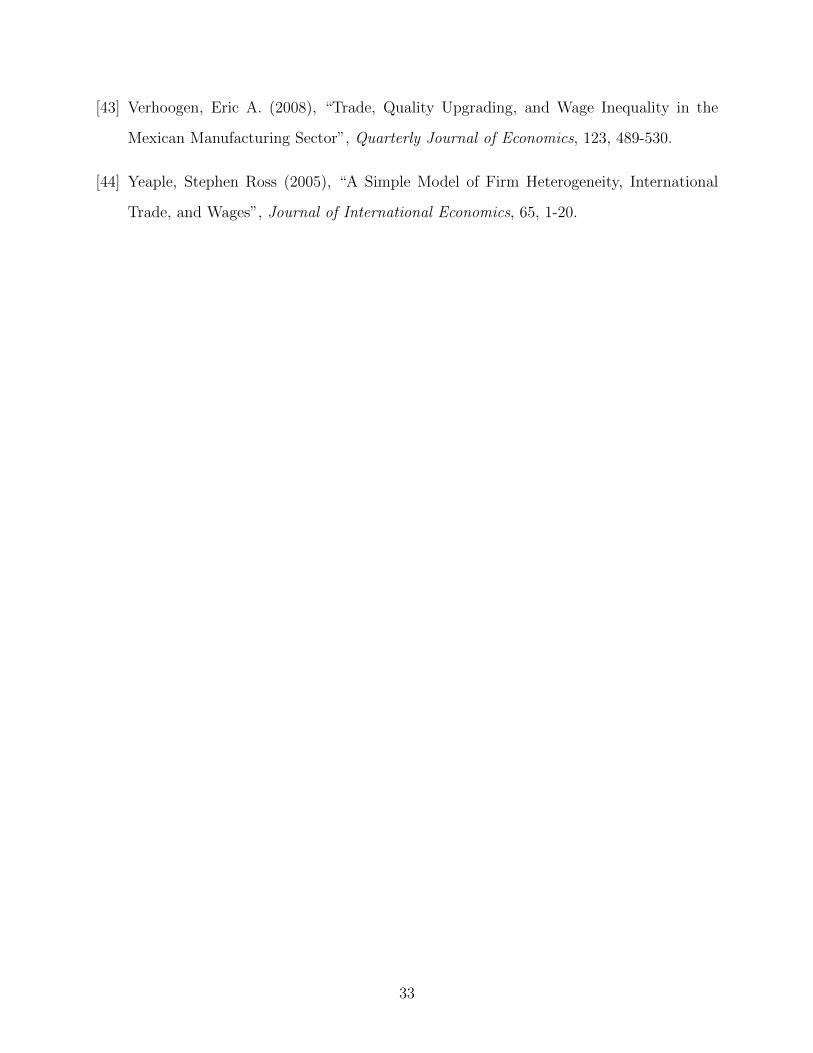
What about the impact on the middle-income class? To derive a clear-cut answer to this
question, we assume now that the individual ability follows the Pareto distribution with its
cumulative distribution function of G(a) = 1 − (a0/a)k, where a0 > 0 and k > 1.7 Then,
it can be shown that under the mild condition σ > 2, international trade decreases the real
wages for the middle-income class, as Figure 5 shows.8 The proof of the following proposition
requires some calculations and is thus relegated to the Appendix.
7It has been documented that both firm size (measured by employment) and upper-tail income distributioncan be approximated by the Pareto distribution with its exponent of 1 for the former and 1.5-3 for the latter(e.g., Atkinson, et al., 2011; and Gabaix, 2009). When the ability is distributed according to a Paretodistribution in our model, so are the firm size and the upper-tail income distribution, which justifies ourchoice of the Pareto as the ability distribution.
8Many authors have estimated the elasticity of substitution and have reported the estimated values thatexceed 2 in most cases; the estimate of the elasticity by Bernard, et al. (2003), for example, is 3.79. Brodaand Weinstein (2006) estimate the elasticities of substitution for different industries at different levels ofaggregation for different periods of time. Table IV of their paper shows that during 1990-2001, the simpleaverage of the elasticities of substitution is 6.6 (with an outlier dropped) for five-digit (SITC) industries; itis 4.0 for three-digit (SITC) industries.
15
Proposition 4 Suppose that there are two symmetric countries in which workers’ ability
distribution follows a Pareto distribution. Then, the lowest income earners who work as
production workers as well as the highest income earners who work as knowledge workers
are better off by international trade. Those who belong to the middle-income class, however,
experience a decrease in real wages by opening to trade: there is a range of workers’ ability
such that the real wages of workers whose abilities are within this range fall as a result of
opening to trade if and only if σ > 2 holds. All knowledge workers who work in the firms
that only serve their individual domestic markets in the trade equilibrium belong to such
middle-income class.
An individual that belongs to the middle-income class (e.g., knowledge workers with a ∈
[α∗T , αX ]) benefits from trade as a consumer due to an increase in the quality index, but loses
as a residual claimer of the firm, since an increase in the quality index leads to a decrease in
the firm’s operating profits. The latter effects outweighs the former if and only if σ > 2, i.e.,
the elasticity of substitution is large enough that the latter competition-enhancing effect is
dominant.
Having derived the impact of trade on individual workers’ real wages, we now turn to
the impact on the overall social welfare of each country. We use two measures of social
welfare to evaluate the effect of international trade: the utilitarian social welfare and the
Lorenz domination. If the ability is distributed according to a Pareto distribution, we have
unambiguous results regarding the impact of trade on social welfare in both measures.
The following proposition–the proof of which is relegated to the Appendix–shows that
trade unambiguously increases a simple aggregation of individuals’ utilities.
Proposition 5 Suppose that there are two symmetric countries in which workers’ ability
distribution follows a Pareto distribution. Then, international trade unambiguously improves
utilitarian social welfare for individual countries.
The other measure of social welfare is the Lorenz domination, which is a measure to
16
evaluate the equality of income distribution. We define the Lorenz function by
L(a) =
∫ a0w(a′)dG(a′)∫∞
0w(a′)dG(a′)
,
the fraction of total income earned by those who have the ability a or less. We say that the
income distribution characterized by the Lorenz function LA is Lorenz-dominated by the one
characterized by LB, if LA(a) ≤ LB(a) for any a with strict inequality for some a.
Proposition 6 Suppose that there are two symmetric countries in which workers’ ability
distribution follows a Pareto distribution. Then, the income distribution under international
trade is Lorenz-dominated by the one in autarky.
The Appendix shows the proof of Proposition 6.
Propositions 5 and 6 give us a clear and important message about the impact of inter-
national trade on income distribution. International trade benefits a country as a whole,
but increases income inequality within the country. This message is reminiscent of the well-
known results from the traditional, neoclassical trade theory: international trade benefits all
trading countries but creates winners and losers within them (the Stolper-Samuelson theo-
rem). But there is an important difference. In traditional trade models, trade increases the
reward to the factor whose reward has been suppressed due to its abundant supply, while
it decreases the reward to the factor that had enjoyed a relatively high reward due to its
scarceness. In contrast, our model predicts a widening of the income gap such that the
reward to the scarce talent that had already claimed a disproportionately large share of the
aggregate income increases even further as a result.
5 Asymmetric Countries
In this section, we extend the baseline model to one where the countries have asymmetric
populations or ability distributions. We will show numerically that our main result that
only the middle-income class suffers from trade liberalization remains valid also in the case
of asymmetric countries. We also show that, among other things, income inequality worsens
17
in both countries as openness to trade increases, but it does so particularly in the smaller
country.
We examine the two cases (i) one in which country 1 is larger than country 2 (i.e., L1 >
L2), and (ii) one in which country 1 has relatively more high-ability workers than country
2. The second case is characterized by the first-order stochastic dominance of the Pareto
distributions for workers’ ability. Specifically, we assume that k1 < k2 so that G1(a) < G2(a)
for any a > a0, where Gi(a) = 1− (a0/a)ki .
We choose production labor in country 2 as the numeraire. The wage rate for the pro-
duction workers in country 1, denoted by w, can be different from 1, while in country 2 it
equals 1. Throughout this numerical analysis, we select σ = 4, l = 1, fX = 1, and a0 = 1
for concreteness when we show our results graphically. The properties of the equilibrium,
however, are robust to changes in parameter values.
The online appendix shows seven equilibrium conditions: free-entry conditions, export-
cutoff conditions, and labor-market clearing conditions for the two individual countries, as
well as the trade balance condition.
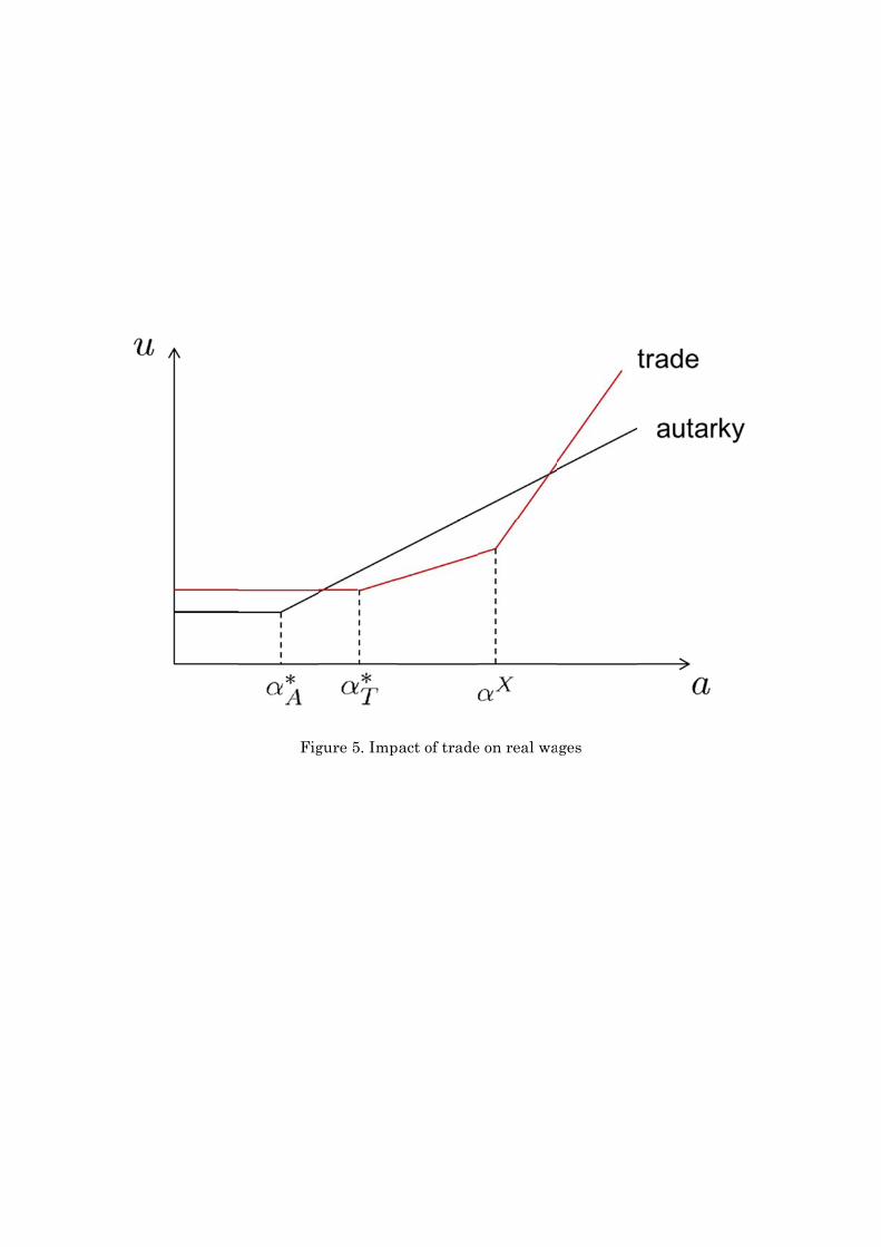
5.1 Different Population
We first consider the case in which the two countries are different only in population size.
We assume that country 1 is larger than country 2: L1 = 100 and L2 = 50. The ability
distributions are the same between the two countries: k1 = k2 = 2.
Figure 6 illustrates the simulation result of the impact of international trade on real wages,
measured by the indirect utility given by (8) in the case of autarky and measured similarly
in the case of the trade equilibrium when the openness to trade, defined by φ = τ 1−σ, equals
0.58 (i.e., τ ≈ 1.2). The first observation we want to emphasize is that in both countries,
only the middle-income class suffers from opening to trade. That is, the main result from
the case of symmetric countries is also valid in this case of asymmetric population size.
As for the comparison between the two countries, we first note that in autarky, the real
wage is higher in country 1 than in country 2 for any ability a. This is because country 1 as
18
the larger country hosts more firms, each of which produces a variety that is slightly different
from others, so that the price index is smaller (or equivalently, the quality index is greater)
in country 1. This advantage of living in the larger country remains even after opening to
trade. We observe (but do not show here) that the wage rate is greater in the larger country
1 than in country 2 (i.e., w > 1), which is known as the home market effect (Krugman,
1980, 1991). Together with the observation that the price index is smaller in country 1
than in country 2, the real wage is still higher in country 1 than in country 2 in the trade
equilibrium for any ability level. In addition, in all simulations with different parameter
values, the results indicate that I1/w and I2 take the same values, respectively, throughout
a change in φ(= τ 1−σ) from 0 to 1. Together with the observation that w > 1, this means
that international trade creates a (nominal) income gap between the two countries, favoring
the larger country.
We also infer from Figure 6 that international trade worsens income inequality, as ob-
served in the symmetric-country case, and it does so more severely for the smaller country.
Our model, like Melitz’s (2003), possesses the important property that the entry threshold
α∗i increases while the export threshold αXi decreases as the openness to trade φ increases,
even when the countries are asymmetric. Compared with the case of autarky, in particular,
the entry threshold in the trade equilibrium is higher and the (nominal) wage schedule shifts
in both countries as indicated in Figure 4. Together with the observation that the values of
I1/w and I2 do not change by opening to trade, this means that the same logic as used in the
proof of Proposition 6 (in the Appendix) applies here, and we can conclude that the income
distribution under international trade is again Lorenz-dominated by the one in autarky, even
in this case. This logic can also be applied to the difference between the countries in as-
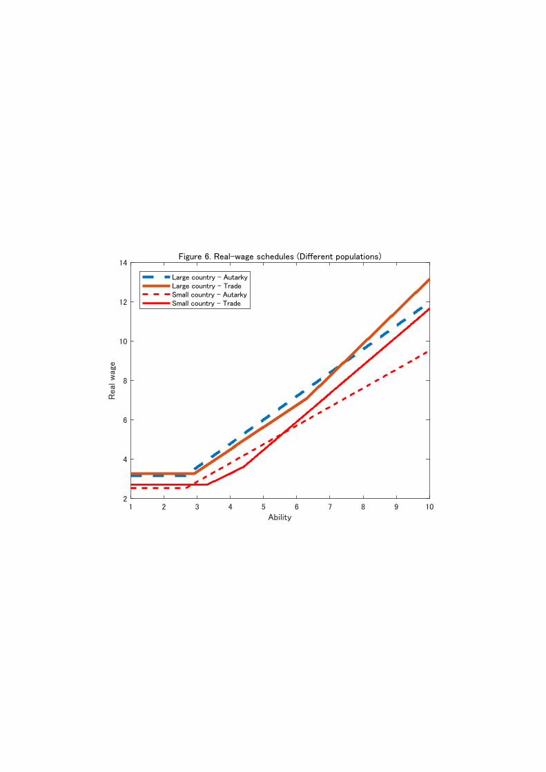
sessing the effect of opening to trade. As Figure 6 indicates, α∗1 < α∗2 and αX1 > αX2 in the
trade equilibrium. The larger country 1 has a larger market than country 2 not just because
of its size but also because of the greater equilibrium wage rate. Consequently, country 1
can accommodate more lower-quality firms (both domestic and foreign) than country 2–i.e.,
α∗1 < α∗2 and αX2 < αX1 – which in turn means that the proportions of both lowest and highest
19
income groups are larger in country 2 than in country 1. Thus, we infer that the smaller
country 2’s income inequality worsens compared with country 1’s in the sense of the Lorenz
domination. This observation is confirmed by Figure 7, which illustrates the vertical differ-
ence between the Lorenz curve in the trade equilibrium and that in autarky, i.e., the income
share in the trade equilibrium minus that in autarky, for countries 1 and 2.
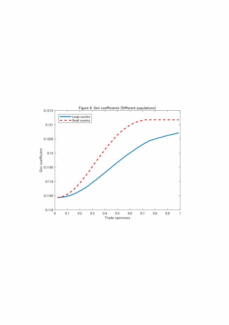
Finally, we find that the income inequality monotonically worsens in both countries as
the openness to trade increases, as expected from the observation that α∗i increases while αXi
decreases with φ. Figure 8 shows that the Gini coefficients increase in both countries as φ (the
openness to trade) increases.9 Moreover, the smaller country 2 always experiences greater
income inequality than the larger country 1. International trade entails job polarization,
which exacerbates income inequality. The smaller the country, the stronger the effect.
A simple empirical analysis using the data from the OECD countries in the period of
1979-2014 gives a weak support of this finding. As shown in the online appendix, we regress
a change in the Gini coefficient on a change in the total value of the country’s international
trade and the interaction term of the total value of trade with the country size, measured
by population. The regression result, based on column (4) in the appendix table (which
includes both country and year fixed effects), indicates that trade increases income inequality
but less so in larger countries, as predicted in the model. However, none of these effects are
statistically significant even at the 10% level.10
5.2 Different Ability Distributions
We turn to the case where the two countries are different only in their ability distribution. We
report the findings here when k1 = 3 and k2 = 4: country 1 has relatively more workers with
high abilities than country 2. We assume that the two countries have the same population:
L1 = L2 = 100.
9All firms in country 2 export their products (i.e., a∗2 = aX2 ), when the openness to trade is greaterthan φ = 0.76 (i.e., τ ≈ 1.10). We observe that country 2’s threshold ability a∗2(= aX2 ) and hence its Ginicoefficient remain the same, respectively, beyond that critical level of openness.
10Alternatively, we may use the 90-10 percentile wage ratio instead of the Gini coefficient to measure incomeinequality, or use the GDP instead of population to measure the size of the countries. The data availability,especially for one that measures income inequality, limits the power of rejecting the null hypothesis.
20
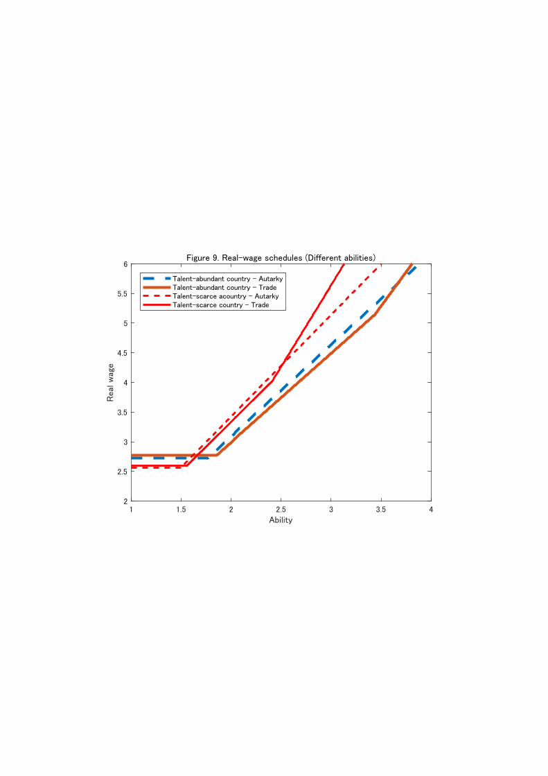
Similarly to the case of population asymmetry, only the middle-income class suffers from
trade in both countries, as Figure 9 shows. We also observe that the real wage for production
workers is greater in the talent-abundant country 1 than in country 2, regardless of whether
the two countries engage in trade. This is because country 1 has more firms that produce
high-quality goods than country 2, so that demands for production workers are higher. When
we compare knowledge workers with the same ability, however, their real wages are higher in
country 2 due to its scarcity of talent; the (nominal) wage for production workers is lower in
country 2 than in country 1 so that the firms in the former earn more operating profits than
their counterparts in the latter. We emphasize here that the fact that knowledge workers
with the same ability earns more in country 2 than in country 1 does not mean that country
2 is wealthier than country 1. Indeed, as Figure 10 indicates, the (nominal) wage is higher in
the talent-abundant country 1 than in country 2 at any percentile of individuals, reflecting
the difference in the ability distributions; individuals at the 90th percentile, for example,
have the ability a = 2.15 and earn w = 1.24 in country 1 while their counterparts have the
ability a = 1.77 and earn w = 1.14 in country 2.
Again, international trade exacerbates income inequality within the countries; Figure 11
indicates that in both countries, the income distribution under the trade equilibrium when
φ = 0.58 is Lorenz-dominated by that in autarky. Indeed, as Figure 12 shows, income
inequality, measured by Gini coefficient, worsens in both countries as the openness to trade
increases.11 Figure 12 also indicates that talent-abundant country 1 always experiences
greater income inequality, as a consequence of a thicker talented population that earns
disproportionately high incomes.
6 Conclusion
In order to examine the impact of international trade on income inequality across workers
with different abilities, we have built a two-country trade model in which the average ability of
knowledge workers determines the quality of the product that the firm produces. Knowledge
11We observe a∗2 = aX2 when φ ≥ 0.98 (i.e., τ is approximately less than 1.01). In such cases, the entrythreshold and hence the Gini coefficient are the same, respectively, over different values of φ.
21
workers are sorted into firms according to their abilities, which entails firm heterogeneity in
product quality. International trade benefits the firms that produce high-quality products,
while it decreases the profits for those that barely export their products and those that serve
only their individual domestic markets. Consequently, income inequality expands among
knowledge workers, the residual claimers of the firms’ profits. International trade increases
the real wages for top income earners and for lowest income earners, who benefit from a
resulting fall of the price index, while it decreases those for the middle-income class.
We have deliberately designed the model as simply as possible in order to highlight what
we believe are the important factors in explaining why globalization entails job and wage
polarization especially in developed countries: the winner-take-all market and the war for
talent. For that purpose, we have made some simplifying assumptions, such as (i) firms
are required to hire only a fixed number of knowledge workers; and (ii) production workers’
productivity does not vary with their abilities. Some of our results would surely be modified
if we relax these assumptions.
In the online appendix, for example, we have analyzed the case in which production
workers’ productivity varies with their abilities. In such cases, the wage inequality naturally
arises among production workers, as well as among knowledge workers. We have shown that
our main message that trade entails wage polarization also remains valid in the extended
model as long as productivity is only modestly dependent on ability. If the ability signifi-
cantly affects their productivity, however, everyone will benefit from trade including workers
in the middle-income. This result is not very surprising because in such cases the wage
increases along with ability almost linearly for the entire population of workers, so that the
difference between knowledge and production workers is minimal, and so that occupational
change from the former to the latter does not lead to a large wage decline.
We have abstracted from the differential effects of international trade on individuals’
real wages through its impact on the relative prices for goods. Broda and Romalis (2009)
document that the relative prices of low-quality products, which tend to be more often con-
sumed by the poor, decline in the US during 1994-2005. Fajgelbaum and Khandelwal (2016)
22
estimate a non-homothetic gravity equation derived from a non-homothetic demand system
and show that trade typically favors the poor, who spend relatively more on traded goods.
We have theoretically derived the result where the lowest-income earners benefit from trade
due to a trade-induced decline in the effective price index of their consumption basket, which
provides another reason (complementary to the above empirical findings) why the lowest-
income earners are likely to benefit from trade. Moreover, trade induces the firms that
produce lowest-quality products to exit the market and hence raises the average quality of
products even for lowest-income earners who may consume relatively more low-quality prod-
ucts. Of course, for a rigorous analysis of the impact of trade on heterogeneous individuals
with different consumption behavior, we need to adopt non-homothetic preferences, as Fa-
jgelbaum et al. (2011) does in order to analyze the impact of trade when goods are vertically
as well as horizontally differentiated. Their framework, together with the aforementioned
extended model illustrated in the online appendix, would also allow us to analyze further
interaction between production and consumption sides when knowledge workers have com-
parative advantage in raising product quality while consuming high-quality products more
than lower-income earners. We leave such an extension as an important issue for future
research.
Our basic message remains largely valid even if we accommodate those features in the
model. Globalization has created the opportunity for firms to reach people all over the world.
Top-tier firms are the main beneficiaries of the globalization since the resulting increases in
sale and profits are large. But other firms are likely to lose because of foreign top-tier firms’
penetration in their own markets. These differential impacts of globalization on firms directly
entail differential impacts on wages of knowledge workers as residual claimers. The most
talented workers who work in top-tier exporting firms benefit from globalization, earning
higher real wages than before. Those who are mediocre knowledge workers are likely to lose;
their firms may suffer from increased competition in their domestic markets, or they may
even drop out of a knowledge-worker pool.
23
Appendix
Proof of Proposition 4. First, we prove that international trade makes the production
workers better off by showing that the product quality index increases (or equivalently, the
price index drops) by trade. Then, we show that trade also makes top income earners better
off. Finally, we derive the condition under which there exist workers with intermediate
abilities, such that their real wages fall as a result of opening to trade.
To calculate the utility in autarky (expressed by (8)) and its counterpart in the trade
equilibrium, we first derive the product quality indices as∫ ∞α∗A
αf(α)dα =kak0L
l
∫ ∞α∗A
α−kdα =kak0L
(k − 1)lα∗k−1A
(16)
in autarky, and∫ ∞α∗T
αf(α)dα + τ 1−σ∫ ∞τσ−1fX
lα∗T
αf(α)dα =kak0L
(k − 1)lα∗k−1T
[1 + τ k(1−σ)
(l
fX
)k−1]
(17)
in the trade equilibrium.
Now, we solve the autarkic FE and LM equations, (6) and (7), for α∗A and IA. Substituting
the expression of (16) into (6), we obtain the aggregate income in autarky as
IA =σl
α∗A× kak0L
(k − 1)lα∗k−1A
=σkL
k − 1
(a0
α∗A
)k. (18)
Then, we substitute (18) into (7) to obtain
l × L
l
(a0
α∗A
)k+
(σ − 1
σ
)σkL
k − 1
(a0
α∗A
)k= L
L
(a0
α∗A
)k (σk − 1
k − 1
)= L,
which gives us
α∗A = a0
(σk − 1
k − 1
) 1k
. (19)
Note that α∗A > a0 holds because σ > 1. We also obtain IA by substituting (19) back to
(18):
IA =σkL
k − 1× k − 1
σk − 1=
σkL
σk − 1. (20)
24
Let us turn to the trade equilibrium. Substituting the expression of (17) into the FE
condition (13), we obtain the aggregate income in the trade equilibrium as
IT =σkL
k − 1
(a0
α∗T
)k [1 + τ k(1−σ)
(l
fX
)k−1]. (21)
Then, we substitute (21) into the LM condition (14) to obtain
l × L
l
(a0
α∗T
)k+ fX ×
L
l
(α0
α∗T
)k (l
τσ−1fX
)k+
(σ − 1
σ
)σkL
k − 1
(a0
α∗T
)k [1 + τ k(1−σ)
(l
fX
)k−1]
= L,
which is reduced to
L
(a0
α∗T
)k [1 + τ k(1−σ)
(l
fX
)k−1](
σk − 1
k − 1
)= L.
Thus, we have
α∗T = a0
[1 + τ k(1−σ)
(l
fX
)k−1] 1k (
σk − 1
k − 1
) 1k
. (22)
Substituting (22) back to (21), we obtain
IT =σkL
k − 1× k − 1
σk − 1×
[1 + τ k(1−σ)
(l
fX
)k−1]−1
×
[1 + τ k(1−σ)
(l
fX
)k−1]
=σkL
σk − 1. (23)
It is immediate from (20) and (23) that IA = IT .
Since the production workers’ wage is normalized to 1, it is obvious from (8) and (15)
that they are better off by opening to trade if and only if the quality index increases by
trade, i.e., ∫ ∞α∗T
αf(α)dα + τ 1−σ∫ ∞τσ−1fX
lα∗T
αf(α)dα >
∫ ∞α∗A
αf(α)dα. (24)
Now, it follows from (16) and (19) that∫ ∞α∗A
αf(α)dα =ka0L
(k − 1)l
(k − 1
σk − 1
) k−1k
. (25)
25
Similarly, we obtain from (17) and (22) that∫ ∞α∗T
αf(α)dα + τ 1−σ∫ ∞τσ−1fX
lα∗T
αf(α)dα
=ka0L
(k − 1)l
(k − 1
σk − 1
) k−1k
[1 + τ k(1−σ)
(l
fX
)k−1] 1k
. (26)
The direct comparison between (25) and (26) reveals that (24) holds, and hence the produc-
tion workers are made better off by international trade.
Next, we show that the highest income earners are better off by opening to trade. As
Figure 5 suggests, we need only show that u′T (a) > u′A(a) for a > αX . Since wA(a) = π(a)/l
for a ≥ α∗A, where π is defined by (5), and wT (a) = [πd(a) + πX(a) − fX ]/l for a ≥ αX , we
obtain from (5), (8), (9), (10), and (15) that
uA(a) =(σ − 1)aIA
lσ2[∫∞
α∗Aαf(α)dα
]σ−2σ−1
for a ≥ α∗A, (27)
uT (a) =σ − 1
lσ[∫∞
α∗Tαf(α)dα + τ 1−σ
∫∞αXαf(α)dα
] 11−σ
×
a(1 + τ 1−σ)IT
σ[∫∞
α∗Tαf(α)dα + τ 1−σ
∫∞αXαf(α)dα
] − fX for a ≥ αX . (28)
Note that the higher the product quality index, the higher a knowledge worker’s utility in
both autarky and trade, when 1 < σ < 2. The higher the quality index, the better off a
knowledge worker will be as a consumer, but the worse off they will be as a residual claimer
of a firm that competes with other firms. The former effect outweighs the latter if and only
if σ < 2, i.e., the elasticity of substitution is small enough that there is only a small negative
impact of an increase in the quality index on the firm’s operating profits.
Now, it follows from (27) and (28) that we have u′T (a) > u′A(a) if and only if[∫∞α∗Tαf(α)dα + τ 1−σ ∫∞
αXαf(α)dα∫∞
α∗Aαf(α)dα
]σ−2σ−1
< 1 + τ 1−σ,
where we have used IA = IT . The expression in the square brackets on the left-hand side is
greater than 1, as we have shown above. Thus, this inequality is satisfied if σ ≤ 2. To see if
26
this inequality is also satisfied even if σ > 2, we rewrite this inequality using (12), (16), and
(17) as [(α∗Aα∗T
)k−1
+
(α∗AαX
)k−1
τ 1−σ
]σ−2σ−1
< 1 + τ 1−σ. (29)
Now, it follows from α∗A < α∗T < αX and k > 1 that(α∗Aα∗T
)k−1
+
(α∗AαX
)k−1
τ 1−σ < 1 + τ 1−σ.
Since 0 < (σ− 2)/(σ− 1) < 1 when σ > 2 and (α∗A/α∗T )k−1 + (α∗A/α
X)k−1τ 1−σ > 1 (which is
equivalent to (24)), we have[(α∗Aα∗T
)k−1
+
(α∗AαX
)k−1
τ 1−σ
]σ−2σ−1
<
(α∗Aα∗T
)k−1
+
(α∗AαX
)k−1
τ 1−σ < 1 + τ 1−σ,
so that we have shown that (29) holds, and hence that the higher income earners benefit
from trade regardless of the value of σ ∈ (1,∞).
Finally, we derive the condition under which the middle-income earners are made worse
off by trade. In the trade equilibrium, the utility of a knowledge worker with a ∈ (α∗T , αX)
can be written as
uT (a) =(σ − 1)aIT
lσ2[∫∞
α∗Tαf(α)dα + τ 1−σ
∫∞αXαf(α)dα
]σ−2σ−1
.
Using IA = IT , we compare this utility with uA(a), shown in (27), to find that uA(a) > uT (a)
for a ∈ (α∗T , αX) if and only if[∫ ∞
α∗A
αf(α)dα
]σ−2σ−1
<
[∫ ∞α∗T
αf(α)dα + τ 1−σ∫ ∞αX
αf(α)dα
]σ−2σ−1
.
It follows from (24) that this inequality holds, and hence opening to trade makes the middle-
income class worse off, if and only if σ > 2.
Proof of Proposition 5. It follows directly from (8) and (15) that each country’s utilitarian
27
social welfare can be written as
SWA =(σ − 1)IA
σ[∫∞
α∗Aαf(α)dα
] 11−σ
,
SWT =(σ − 1)IT
σ[∫∞
α∗Tαf(α)dα + τ 1−σ
∫∞αXαf(α)dα
] 11−σ
.
Thus, trade improves utilitarian social welfare if and only if
IA[∫∞α∗Aα′f(α′)dα′
] 11−σ
<IT[∫∞
α∗Tα′f(α′)dα′ + τ 1−σ
∫∞τσ−1fX
lα∗T
α′f(α′)dα′] 1
1−σ,
which is satisfied since IA = IT , as shown in the proof of Proposition 4, and the product
quality index is greater in the trade equilibrium than in autarky, as shown in (24).
Proof of Proposition 6. Recall that the equilibrium wage schedules in autarky and in
trade are given by
wA(a) =
1 for a ∈ [0, α∗A)aα∗A
for α ∈ [α∗A,∞)
and
wT (a) =
1 for a ∈ [0, α∗T )aα∗T
for a ∈ [α∗T , αX)
aα∗T
+ (a−αX)fXlαX
for a ∈ [αX ,∞),
respectively. It follows from α∗A < α∗T < αX that there exists α (> αX) such that (i)
wT (α) = wA(α); (ii) wT (α) ≤ wA(α) for all α ≤ α; and (iii) wT (α) > wA(α) for all α > α, as
depicted in Figure 4. This implies that LA(a) = LT (a) for all a ≤ α∗A, and LA(a) > LT (a)
for all a > α∗A, since wA(a) = wT (a) = 1 for a ≤ α∗A and∫∞
0wA(a)dG(a) =
∫∞0wT (a)dG(a),
which is shown in the proof of Proposition 4 as IA = IT . Thus, the income distribution
under international trade is Lorenz-dominated by the one in autarky.
28
References
[1] Acemoglu, Daron and David Autor (2011), “Skills, Tasks and Technologies: Implica-
tions for Employment and Earnings”, Handbook of Labor Economics 4(B), 1043-1171,
Elsevier.
[2] Acemoglu, Daron and James A. Robinson (2006), Economic Origins of Dictatorship
and Democracy, Cambridge University Press, New York.
[3] Atkinson, Anthony B., Thomas Piketty, and Emmanuel Saez (2011), “Top Incomes in
the Long Run of History”, Journal of Economic Literature, 49, 3-71.
[4] Autor, David H. and David Dorn (2013), “The Growth of Low-Skill Service Jobs and
the Polarization of the US Labor Market”, American Economic Review, 103, 1553-1597.
[5] Autor, David H., David Dorn, and Gordon H. Hanson (2013), “The China Syndrome:
Local Labor Market Effects of Import Competition in the United States”, American
Economic Review, 103, 2121-2168.
[6] Autor, David H., David Dorn, Gordon H. Hanson, and Kaveh Majlesi (2017), “Im-
porting Political Polarization? The Electoral Consequences of Rising Trade Exposure”,
NBER Working Paper 22637.
[7] Autor, David H., Lawrence F. Katz, and Melissa S. Kearney (2006), “The Polarization
of the U.S. Labor Market”, American Economic Review Papers and Proceedings, 96,
189-194.
[8] Autor, David H., Lawrence F. Katz, and Melissa S. Kearney (2008), “Trends in U.S.
Wage Inequality: Revising the Revisionists”, Review of Economics and Statistics, 90,
300-323.
[9] Autor, David H., Frank Levy and Richard J. Murnane (2003), “The Skill Content of
Recent Technological Change: An Empirical Exploration”, Quarterly Journal of Eco-
nomics, 118, 1279-1333.
29
[10] Baumgarten, Daniel (2013), “Exporters and the Rise in Wage Inequality: Evidence
from German Linked Employer-Employee Data”, Journal of International Economics,
201-217.
[11] Bernard, Andrew B., Jonathan Eaton, J. Bradford Jensen, and Samuel Kortum (2003),
“Plants and Productivity in International Trade”, American Economic Review, 93, 1268-
1290.
[12] Bernard, Andrew B. and J. Bradford Jensen (1997), “Exporters, Skill Upgrading, and
the Wage Gap”, Journal of International Economics, 42, 3-31.
[13] Blanchard, Emily and Gerald Willmann (2016), “Trade, Education, and the Shrinking
Middle Class”, Journal of International Economics, 99, 263-277.
[14] Blau, Francine D. and Lawrence M. Kahn (1996), “International Differences in Male
Wage Inequality: Institutions versus Market Forces”, Journal of Political Economy, 104,
791-837.
[15] Broda, Christian and David E. Weinstein (2006), “Globalization and the Gains from
Variety”, Quarterly Journal of Economics, 121, 541-585.
[16] Broda, Christian and John Romalis (2009), “The Welfare Implications of Rising Price
Dispersion”, unpublished manuscript, University of Sydney.
[17] Burstein, Ariel and Jonathan Vogel (2010), “Globalization, Technology, and the Skill
Premium: A Quantitative Analysis”, NBER Working Paper 16459.
[18] Caliendo, Lorenzo, and Esteban Rossi-Hansberg (2012), “The Impact of Trade on Or-
ganization and Productivity”, Quarterly Journal of Economics, 127, 1393-1467.
[19] Card, David, Jorg Heining, and Patrick Kline (2013), “Workplace Heterogeneity and the
Rise of West German Wage Inequality”, Quarterly Journal of Economics, 128, 967-1015.
[20] Costinot, Arnaud and Jonathan Vogel (2010), “Matching and Inequality in the World
Economy”, Journal of Political Economy, 118, 747-786.
30
[21] Danziger, Eliav (2017), “Skill Acquisition and the Dynamics of Trade-Induced Inequal-
ity”, Journal of International Economics, 107, 60-74.
[22] “Executive Pay: Bosses under Fire”, The Economist, January 14th-20th 2012.
[23] Egger, Harmut and Udo Kreickemeier (2012), “Fairness, Trade, and Inequality”, Journal
of International Economics, 86, 184-196.
[24] Fajgelbaum, Pablo D., Gene M. Grossman, and Elhanan Helpman (2011), “Income
Distribution, Product Quality, and International Trade”, Journal of Political Economy,
119, 721-765.
[25] Fajgelbaum, Pablo D. and Amit Khandelwal (2016), “Measuring the Unequal Gains
from Trade”, Quarterly Journal of Economics, 131, 1113-1180.
[26] Friedrich, Benjamin (2016), “Internal Labor Markets and the Competition for Manage-