A Work Project, presented as part of the requirements for the Award of a Masters Degree in Finance from the NOVA – School of Business and Economics. Internship Report A Guide to Structured Products – Reverse Convertible on S&P500 Tiago Alexandre Costa Neves Paixão Student Number: 310 A Project carried out under the supervision of Professor Miguel Ferreira.
Transcript
A Work Project, presented as part of the requirements for the Award of a Masters Degree
in Finance from the NOVA – School of Business and Economics.
Internship Report
A Guide to Structured Products – Reverse Convertible on S&P500
Tiago Alexandre Costa Neves Paixão
Student Number: 310
A Project carried out under the supervision of Professor Miguel Ferreira.
2
Internship Report
A Guide to Structured Products – Reverse Convertible on S&P500
Prelude
The following report is presented as a requirement for the award of the Masters in
Finance degree from Nova – School of Business and Economics. It is the outcome of an
internship in Nomura International on the Equity Derivatives Sales division and represents
part of the work and concepts learned during its duration.
Abstract
The purpose of this report is to describe the main characteristics of structured products.
These products can be divided in Capital Guaranteed products and Non Capital guaranteed
products, having these two types of products different risk profiles and potential returns. In
the final part of the report a Reverse Convertible on the S&P500 is created, which offers
8.57% return per year subject to a capital loss in case the underlying goes below 70%
initial level, in one year.
Keywords: {Down and in Put; Reverse Convertible; Delta; Gamma}
3
Summary
Part 1
Introduction 4
Capital Guaranteed Notes 6
Non Capital Guaranteed Notes 7
Part 2
Literature Review 10
Methodology 11
Pricing 11
Hedging 13
Coupons and Financing 17
Margin and Re-offer 17
Reverse Convertible on S&P500 18
Conclusion 21
References 22
Annex 23
4
Introduction
Over the last decades, the world has been assisting to a truly outstanding evolution in the
financial markets. Products have become more complex and investors more demanding.
Thus, investment opportunities have evolved, and new types of products have been created
has a response to this evolution.
The goal of this report is to analyze structured products linked to equity. In the first part
of the report a brief description and general approach to structured products will be made.
The second part will consist in the analysis of the pricing and hedging properties of a
specific structured product called reverse convertible.
A structured product is an investment product that comprises characteristics of both
equity and fixed income, having upside potential with downside protection. The features of
structured products, such as the maturity, the underlying asset and the payoff, are specified
prior to issuance and remain the same until the end of the product’s maturity.
The market of structured products started with the development of the derivatives market
in the nineties. These investments first arose with the need for companies to issue bonds
and finance themselves. In order to get cheaper financing, companies started to issue
convertible bonds (which are bonds that at a certain point in time can be converted to
stocks). Then, investment banks decided to add other characteristics to these convertible
bonds that would link the payoff of the investment to other underlying assets such as
equity. In sum, structured products are made of strategies that combine different types of
derivatives with other assets and are sold as a single product.
From an investor point of view, structured products can have advantages relative to other
investment products. For example, in terms of tax efficiency, structured products can
benefit from lower tax rates depending on the country of issue. Moreover, these products
can be adapted to different types of investors and different maturities, as the investment
5
banks that sell them have the scale and capacity to tailor a product for a specific investor.
This characteristic makes this type of products very interesting to investors, since they can
personalize the payoff, the underlying assets and all the terms according to their needs. For
example, for very risk-averse investors, products with capital protection can be made and
sold as bonds. On the other hand, for less risk-averse and directional investors, products
linked to the underperformance of the market, as well as products with leverage can be
sold.
However, there are also some disadvantages when comparing these products to other
investment opportunities. Since they are created by financial institutions, the investor
always pays a fee, which is embedded on the price of the product, leading to higher
transaction costs than other assets. Furthermore, the fact that the product is customized is
also a reason for it to be very illiquid and difficult to mark-to-market on a regular basis.
Finally, structured products can have really complex payoffs and exposures, and
sometimes for less experienced investors this can be dangerous. As they are tailored made
by professional investment bankers, there is space for some mismatching between the
investors profile and the product characteristics.
Types of Structures
As previously stated, structured products can have numerous types of payoffs, underlying
assets and mechanisms. The next part of the report analyzes some of those features and
some products are given as examples.
The main distinction among structured products concerns the level of capital protection
of the structure. In this context, two basic categories can be viewed as follows:
Capital Guaranteed (100% or greater, for example 110%);
Non Capital Guaranteed (principal-at-risk with potential for full exposure to the
performance of the underlying asset).
6
Capital Guaranteed Notes
Capital Guaranteed Notes are hybrid securities which combine a fixed income note with a
derivative typically linked to an equities index (or a basket of indices), or other assets. This
type of structure is designed for investors seeking to protect their capital while having the
potential to gain from an increase in the value of an asset. Typically, any increase in a
reference index would be paid out at maturity, although certain index-linked notes may
provide regular coupons.
Investment bank point of view
In order to provide the investor with this product there are two separate things the bank
will do. First, in order to have 100% of the capital at maturity, the bank will put the capital
earning interest in a way that, at maturity, the total capital plus interests is equal to 100%
of the capital employed by the investor. The bank will invest in bonds such that at maturity
the capital will be available with no interest rate risk, for example, zero-coupon bonds or
strips. Second, the bank also has to open an exposure to the underlying, and therefore will
enter into a derivative position such as a call option or any other option strategy that
provides an upside exposure to the underlying. Usually the exposure it is not 100%,
meaning that, with the proceeds, the bank will only be able to purchase a portion of the
option. In sum, the bank will receive 100%, will put 100% - X% earning interest to get
100% at maturity and will use the X% to gain upside exposure to the underlying.
Investor point of view
The big advantage of this structure for the investor is the fact that it has total capital
guarantee. Moreover, it is also an hedge for a moderate drop on the underlying, plus the
possibility of gaining a return over the life of the product. Here, the big drawback is the
opportunity cost of the structure. If the underlying performs badly, the investor will receive
7
only 100% of the capital invested, having therefore an opportunity cost of earning a certain
return elsewhere.
Non Capital Guaranteed Notes
The two most popular types of structure with capital at risk are the auto-callable note and
the reverse convertible note.
1) Auto-callable Note
Auto-callable notes are non-principal protected products that can be linked to the
performance of an underlying stock, basket of stocks or equity index. The main
characteristic of this product is that it can be redeemed before maturity if certain event
happens. The automatic call feature is triggered, usually, if the stock price of the
underlying investment is at or above a certain level during the life of the product.
Considering, for example, a product with maturity of 3 years, with annual observations, if,
at any observation, the underlying asset is above X% initial level1, the investor receives
Y%*n of coupon and the structure is cancelled2. If not, it continues to the next period. This
type of coupon is called a snowball coupon, since it increases with the maturity of product.
On the other hand, if, at maturity (and not early redeemed) the underlying is below Z%3
initial level the investor will not receive a coupon and the notional amount will be paid
according to the underlying performance (NA*underlying performance)4.
Investment bank point of view
In order to structure this product, the investment bank will have to divide the payoffs in
two different legs. First, since the structure promises a coupon payment in case the
1 Coupon trigger level.
2 N stands for the year in which the coupon is paid. In this case can be 1, 2 or 3.
3 Barrier level.
4 NA: Notional Amount: Underlying Performance: Level at maturity/Initial level.
8
underlying is above the coupon trigger level, the bank should calculate the probability of
the coupon being paid5. Then, since the bank will receive the capital from the investor, it
should also be accounted how much will the bank yield by employing the capital in the
market6.
In the other part of the product, the investor may lose part of its capital if the underlying
is below the barrier level. This payoff can be replicated by a put option that only gets
active if the underlying is below Z%7. This type of option is called a barrier option. In this
case, this is a down and in put.
A down and in put option is a type of barrier option that is only activated when the
underlying reaches a certain barrier. It is called down and in because it gets activated (in)
when the underlying reaches a point that is below the strike (down).
In sum, putting these components together, the structure can be sold to investors as an
auto-callable note.
Investor point of view
Although the investor bears the risk of the underlying falling below the barrier level, it
does also yields a high coupon if the product is above the coupon trigger level. On the
other hand, since the coupons are fixed, the investor also forgoes higher returns in the case
the underlying asset moves higher than the coupon level. The payoff of the product is
graphically represented in Annex 1.
5 This is usually done using Monte Carlo simulations.
6 Here it should also be accounted the probability of the structure being cancelled and the bank only receiving
interest up to that moment.
7 It will be further discussed in the report how to price this exotic option.
9
2) Reverse Convertible Note
Reverse Convertible notes are non principal protected products linked to the performance
of an equity underlying. The key idea of this product is that the investor is willing to accept
some downside risk in exchange for an above market coupon.
The reverse convertible note can be decomposed in two different parts. On one hand,
since the investor receives coupons on the principal invested this may be viewed as a
“coupon bond”. On the other hand, the product exposes the investor to a downside risk on
the underlying asset. If the lower pre-specified barrier is hit, the investor will be exposed to
the performance of the underlying and may lose part of the capital invested. This feature of
the product is achieved by a short position in a down and in put option. The investor
receives a coupon periodically and, at maturity, if the underlying equity is below a the
barrier the investor will not receive the total notional employed in the product.
Thus, reverse convertibles provide an effective strategy for yield enhancement by
combining a fixed income security with a short position on a down and in put option. They
are designed to outperform comparable bonds on the upside and outperform the underlying
equity when the underlying equity falls8. The product has characteristics of traditional
fixed income securities, but offers high coupons in return for a downside risk on an equity
underlying.
Concluding, the reverse convertible can be divided in a bond plus a short position9 in a
barrier option. In the next pages of this report it will be analyzed how do investment
banks issue and price those securities. Afterwards, all the mechanics, hedging and pricing
of the reverse convertible will be explained and applied.
8 Although when the underlying falls below the barrier the product does not outperform.
9 The short position is the investor position. The issuer will be long the option.
10
Literature Review
There have been several studies related to structured products among the academic
community. Most of them rely on analytic analysis in how to price exotic options or how
to hedge the exposure to the different greeks of a product. Since the main analysis of this
report regards a reverse convertible, the main focus will be on pricing and hedging a
barrier option (down and in put).
The research on this subject started in the seventies, when Merton (1973) derived a
formula for pricing a knock-out call option. In this paper, the idea consisted in replicating
the payoff of a barrier option using a dynamic strategy.
In terms of barrier option valuation there are two main methods that have been discussed
among academics, the expectations method and the differential equation method.
Subsequent work on pricing continuously monitored barrier options with the expectations
method includes Heynen and Kat (1994), Kunitomo and Ikeda (1992) and Rich (1994).
The expectation pricing method requires that the risk-neutral densities of the underlying
price are determined both above and below the barrier. Then, the price of the option is
derived from the discounted payoff calculated over those densities, however it was
considered analytically difficult to work out the densities in this model and therefore,
closed form solutions for the problem were obtained in the literature.
Concerning the differential equation method, a brief discussion of the method can be
found in Wilmott, DeWynne and Howison (1993). The basic idea is that all barrier options
satisfy the Black-Scholes partial differential equation but with different domains,
expiration and boundary terms. Here, again, the model requires a complex integrals
analysis, and therefore some closed solutions for the problem were obtained. More recently,
closed formulas for barrier options were presented in Hull (1993) and Haug (1997).
11
Barrier options are traded over-the-counter among the biggest financial institutions
worldwide. However, traders on the sell side usually hedge the risks associated with this
position. Therefore, one of the most important topics when referring to barrier options is
the hedging strategy used to eliminate the market risk associated with a long/short position
in the option.
Derman, Ergener and Kani (1995) and Carr, Ellis and Gupta (1996) discussed the static
hedging of barrier options with regular options on the same underlying security. In this
case, a fixed strike strategy is used, in which the replicating portfolio consists of options
with a single strike but multiple expiries.
Duffie and Richardson (1991) presented the “mean-square hedging” method. In this
method the idea was to minimize the hedging residual (the difference between the payoff
of the barrier option and the payoff of a static hedging portfolio). The issue was also
approached by Carr and Chou (1997) who extended the model to make the hedging
portfolio consistent with linear constraints, and introduced a fixed maturity strategy, with a
replicating portfolio composed by options with a single maturity but multiple strikes.
Methodology
On the following part of the report, a reverse convertible will be created. For that purpose,
the main constituents of the product will be individually analyzed. These constituents
comprise a barrier option, the coupons/financing and the margin/re-offer.
Barrier Option
Pricing
In order to price barrier options it is important to clarify some aspects related to this type
of securities. One of the most important aspect is the time frequency of the barrier
monitoring.
12
Barrier triggers can be continuously or discretely monitored. The difference between the
two is that discretely monitored barriers have a fixed date of observation for the trigger, in
contrast to continuous options that can be triggered at any point in time. For example, if, in
a discretely monitored barrier, the barrier is monitored annually, only once a year it will be
checked if the spot price has reached the barrier or not.
For the purpose of this report, it will be necessary to price a discrete option. Therefore, an
adjustment for the discrete monitoring is required.
The Black-Scholes model, is the worldwide model used for option valuation, and a
variation of this model will be used to price the down and in put.
Recalling the historical paper of Black and Scholes (1973) the closed formula for a
vanilla put option can be written as follows10
:
[1]
[2]
[3]
Then, after adapting the model to price a down and in option, the closed formula solution
was presented in Hull (1993) and Haug (1997).
Considering an arbitrage relationship:
Knock in option + Knock out option = Vanilla option
The value of the down and in put should be equal to the value of a vanilla put minus the
value of a down and out put. The closed formula for pricing the option is presented below.
[4]
10 K: Strike; r: Interest rate; q: Dividend yield; S: Spot; σ: Volatility; T: Time to maturity; H: Barrier level
13
Where:
[5]
[6]
[7]
[8]
Adjusting for discrete barriers
As previously said, this closed formula solution is pricing an option that is continuously
monitored. Broadie, Glasserman and Kou (1997) presented an adjustment to the formula
for discrete barrier options. According to the authors, let V(H) be the price of a continuous
barrier option, and V(H’) be the price of an otherwise identical barrier option with
monitoring points. Then we have the approximation:
[9]
With + for an up option and − for a down option, where the constant β =−(ζ(1/2)/√2π) ≈
0.5826, ζ the Riemann zeta function.
Giving the closed formulas presented above, it is possible to price a down and in put for a
reverse convertible note.
Hedging
As already discussed in the report, barrier options are not traded through an exchange as
standardized options or stocks can be. Whenever an investor wants to trade a barrier option
he should find a counterpart that is willing to enter in this contract. This counterpart is
usually an investment bank that provides liquidity to the market through its exotic trading
desks.
However, when the bank issues the derivative and enters in a contract with an investor, it
is not supposed to be exposed to the market risk that the investor is looking for. In other
14
words, investment banks are acting only as market makers of the product and not as the
other part of the bet and therefore hedge their positions to cover its market risk exposure.
In terms of vanilla options, the hedging is quite simple. The bank sells/buys the quantity
of the underlying asset needed to be neutral to market behavior. When buying an option,
the bank does not want to be exposed to changes in the underlying price that affect the
value of the option, therefore it will cover this risk by a method called delta hedging. Since
the delta measures the sensibility of the option price to changes in the underlying, if an
option has a delta of 0.3 and an investor bought 100 options on a specific stock, the bank
should buy/sell 30 stocks in order to be neutral to changes in the stock.
The hedging of the greeks (delta and gamma), in a vanilla option, is relatively simple,
since these parameters are well behaved through the life of the option (see Annex 2 and 3).
In a barrier option (in this case a down and in put), the greeks present a different behavior
(see Annex 4, 5 and 6), therefore, other hedging models should be taken into account.
The two hedging models that will be discussed are the static and the dynamic hedging
models.
Static hedging
As previously mentioned, one of the most popular models in the literature regarding
barrier options hedging was presented by Derman, Ergener and Kani (1995). The model is
known as the DEK model. The DEK model presents a static strategy for the hedging of a
barrier option. The authors created a portfolio of plain vanilla options to replicate the
payoff of a barrier option. This portfolio is such, that it replicates the value of the option
for any change in the underlying for a wide period of time before maturity, since it
decomposes the value of an exotic option into a portfolio of vanilla options.
Carr and Chou (1997) also presented a static hedging strategy in which they create a
replicating portfolio with the same payoff of the barrier option when the spot is at the
15
barrier. With this portfolio, if the barrier is never hit, the portfolio will have 0 payoff. In
the case that at some point during the option maturity the barrier is hit, the portfolio will
have the exact payoff of the barrier option. When this happens, this portfolio would be sold
and the proceeds used to buy vanilla options that provide the same payoff of the barrier
option.
Dynamic hedging
The dynamic hedging model can be viewed as a delta and gamma hedging model. The
delta of an option is not constant through time and therefore the hedging ratio of an option
is constantly changing. Then, in order to be perfectly hedged, the issuer of the option11
, has
to rebalance the stock portfolio often and incur in more trading costs, hedging this way the
gamma of the option.
This is relatively simple for a vanilla option, however, for a barrier option, the gamma
can have huge jumps, which makes the option more difficult to hedge using this model.
Concerning the down and in put that is being analyzed, if the underlying asset goes down,
then the price of the option goes up for two reasons. First, if the price goes down, the
payoff of the option will be higher since the option will be more in the money. Moreover,
the fact that the option will only be active if it hits the barrier does also contribute to the
increase in value of the option (since the underlying value will be closer to the barrier
level).
The delta hedging problems of a barrier option happen when the spot price of the
underlying reaches the barrier. In this case, the sensitivity of the price of the option to the
price of the underlying vary substantially. In the down and in put, a small change in the
underlying can make the option active with a substantial payoff. In the Annex 4,5 and 6
can be seen a graphic representation of the down and in put payoff, delta and gamma.
11 The issuer is the agent that is creating the product and will have to hedge it.
16
In order to smooth the gamma around the barrier, put spreads on the underlying can be
used. A put spread is structured by buying a put and selling a put of the same maturity but
with different strikes.
For example, if the barrier is at 70%, the issuer will be long a 69% strike put and short a
70% strike put. In this case, we say that the barrier shift is 1%. To have the best gamma
hedging, the issuer will have to buy as much put spreads as possible and to have a low
barrier shift. The replication is easier to make when the underlying asset is liquid and not
volatile. The characteristics of this structure in terms of greeks can be seen in Annex 7 and
8.
Thus, in the price of the option the issuer should consider how much it will cost to hedge
the position. For example, by buying a 70% barrier option and applying a 1% shift, he will
be pricing a 69% barrier option in order to account for the change in delta near the barrier,
and the hedging costs that this feature brings. With time decay, the issuer will rebalance his
book in order to account for the change in the greeks of the option.
Static vs. Dynamic
Although both hedging methods are presented and studied among academics, in practice
only one of them is used by practitioners.
In the case of the static hedging, the lack of liquidity of the options in the replicating
portfolio as well as the practical difficulty of selling the portfolio exactly when the barrier
is hit are the main drawbacks of the model, which make it very difficult for traders to use it.
Thus, the dynamic hedging model, in which the options are hedged through theirs greeks,
is the most used hedging strategy for this kind of options.
17
Coupons and Financing
The reverse convertible note offers the investor a fixed coupon. The coupons, in this case,
are unconditional on any direction of the underlying, meaning that, they will be paid no
matter what the market conditions are.
The coupon level of the structure will depend on two important things. First, the investor
will be shorting an option, thus, the premium12
of that option will be incorporated on the
coupon level. Second, since the bank will receive the notional amount from the investor,
there is also an element of funding in the product. The notional amount will be put in the
market, yielding a certain level of interest. As the interests received will be used to finance
the structure, this yield rate is called the funding of the product. Usually, the funding is a
floating rate with a fixed spread (for example Euribor – 10bps).
The investors will receive the premium for their short position in the knock in barrier
option, plus a funding amount regarding the interest on the notional. Those two things
together comprise the coupon level of the product.
Margin and Re-offer
Since the idea of the reverse convertible is to enhance high yield coupons by bearing
downside risk, the value of the downside risk should capitalize on the upside coupons. This
means that the coupon level should equal the funding plus the DIP (down and in put)
premium. If this would happen, the product would be issued at fair value, and the issuer
would not yield any margin. Therefore, there is always a spread on the products in which
the issuer keeps a margin. Thus, in order to calculate the final coupon it should also be
taken into account the margin fee for the issuer.
12 From now on the price of the option will be called premium.
18
Moreover, if the product is being sold to a retailer, meaning that it is being sold to an
institution that will sell it to another client, the issuer can share this percentage of margin
with the product distributor.
For example, if an investment bank is selling a product to a private bank, which will then
sell it to an individual investor, the investment bank can issue the note with a certain
percentage of re-offer, meaning that the percentage left for margin can be shared by the
original issuer and the distributor of the product to the final client.
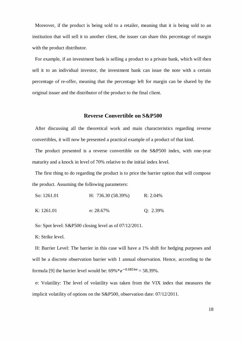
Reverse Convertible on S&P500
After discussing all the theoretical work and main characteristics regarding reverse
convertibles, it will now be presented a practical example of a product of that kind.
The product presented is a reverse convertible on the S&P500 index, with one-year
maturity and a knock in level of 70% relative to the initial index level.
The first thing to do regarding the product is to price the barrier option that will compose
the product. Assuming the following parameters:
So: 1261.01 H: 736.30 (58.39%) R: 2.04%
K: 1261.01 σ: 28.67% Q: 2.39%
So: Spot level: S&P500 closing level as of 07/12/2011.
K: Strike level.
H: Barrier Level: The barrier in this case will have a 1% shift for hedging purposes and
will be a discrete observation barrier with 1 annual observation. Hence, according to the
formula [9] the barrier level would be: 69%* = 58.39%.
σ: Volatility: The level of volatility was taken from the VIX index that measures the
implicit volatility of options on the S&P500, observation date: 07/12/2011.
19
R: Interest Rate: The interest rate level used is the Euribor 1 year as of 07/12/2011.
Q: Dividend Yield: Bloomberg terminal data as of 07/12/2011. The dividend yield is
calculated by a weighted average of the dividends in the S&P500 measured in index points.
Using formula [4] for the pricing of a down and in barrier option, the result is as follows:
DIP = 94.94 = 7.53% of the Spot Value13
After knowing the price of the option it is extremely important to hedge it. In this case,
only the two greeks will be hedged (delta and gamma).
For this, the most commonly used strategy is the put spread. As observed in the Annex 7
and 8, the put spread has almost a binary payoff, and therefore the gamma moves a lot
around the different strikes.
Thus, to hedge the gamma of a down and in put on the S&P500 with a 70% barrier, since
it is already applied in the premium of the barrier option a 1% shift, the put spread with
strikes 69%-70% will be used. The issuer will then buy the 69% strike put and sell the 70%
strike put on the S&P500.
Delta
The delta of this barrier option is, in this case, 0.53. Therefore, in order to hedge the delta
of the option the issuer of the option should buy (0.53*Notional)/(S&P500 level*250)
future contracts on the S&P50014
.
Coupon, Financing and Margins
After having the price of the barrier option, in order to calculate the coupon of the
product there are two major aspects to take in consideration.
The first thing to check is how much interest it will be earned by putting the notional of
the product in the interbank money market. This is extremely important because it reveals
13 (94.9403/1261.01)
14 Each S&P500 future contract has a nominal value of (250*S&P500 level).
20
the capacity of the issuer to have attractive funding for their products. The interest rate
used for this example is the one-year Euribor rate (2.04%).
Thus, having the DIP value (7.53%) and the funding value (2.04%), we could say that
the product will earn a coupon of 9.57%, assuming a 0% margin for the issuer.
However, supposing that the issuer and the distributor are different entities, they will also
incorporate a margin for themselves. If each part takes 0.5% margin on the product, then,
the final coupon of the product would be 8.57%.
The flows between the two parts are summarized in the diagram in the Annex 9, and the
payoff and scenario analysis can be seen in Annex 10 and 11.
To conclude, the investor will receive 8.57% coupon at the end of the year and will bear
the risk of receiving just part of the notional if the S&P500 falls below 70% its initial level.
The issuer and the retailer get 0.5% of the notional as a fee.
21
Conclusion
The appearance of structured products has definitely been a huge improvement and
development for the financial world. These products are suitable for different types of
investors with different risk aversion levels. From capital guaranteed notes to reverse
convertibles, the broad range of different products can easily be accessed by any individual
investor.
The issuer of these products, through its quantitative pricing models, its hedging practice
and capacity, can easily issue any kind of product with any kind of underlying. In the case
of the reverse convertible, it was seen that the issuers of this product use a closed form
solution derived from the Black-Scholes assumptions for the pricing, apply a barrier shift
and hedge themselves by buying put spreads on the underlying. Then, after having the
price of the barrier option, by adding the funding component and subtracting the margin
for the issuer, the coupon level is achieved.
Finally, taking as example a Reverse Convertible on the S&P500, a product was created,
giving the investor a coupon of 8.57% per annum with a 70% downside risk to the index.
In fact, the investor would receive 8.57% the amount invested, and will only receive the
entire notional back if the S&P500 at the end of the year is above 70% initial level,
otherwise, the redemption value will equal the underlying performance. In the end, the
issuer and the retailer of the product would take a 0.5% fee each for the issuing and
distribution work.
22
References
Black, Fischer and Myron Scholes. 1973. The Pricing of Options and Corporate Liabilities.
Journal of Political Economy. 81:637-657.
Bouzoubaa, Mohamed and Adel Osseiran. 2010. Exotic Options and Hybrids. London:
Wiley Finance.
Broadie, Mark, Paul Glasserman and Steven Kou. 1997. A Continuous Correction for