Software and Hardware implementation of an Invariant Feature detector Emmanuel David Bello [email protected]Internship report Company: Robert Bosch GmbH Supervisors: Arne Zender, Robert Bosch GmbH Fernando Ortiz Cuesta, Robert Bosch GmbH 1
Transcript
Software and Hardware implementation of an Invariant Feature detector
This work present the results obtained during the design and implementation, in software and hardware (VHDL), of an Invariant Feature Detector. The implementation of proposed hardware architecture on a Xilinx Virtex-4 FPGA and its evaluation are presented. The software implementation of the detector, which was made in order to test easily our detection algorithm, is also presented. A framework for performance evaluation of feature detectors and descriptors is proposed. The main goal of this work is to achieve a trade-off between hardware resources and performance (in terms of invariance to certain transformations), in the design of the feature detector in hardware.
2.1 Image data set....................................................................................................................................... 8
2.2 Relation between matches and correspondences................................................................................. 10
3.1 General structure of OpenCV library...................................................................................................... 11
3.2 FD_tester class diagram..................................................................................................................... 13
4.1 Relations between SIFT_SWA, SIFT and Feature2D............................................................................ 14
4.1 Smoothing factor of each layer in the Gaussian Pyramid...................................................................... 16
5.1 Found bugs in the initial version of IFD2_HW........................................................................................ 24
5.2 Synthesis results of IFD2_HW............................................................................................................... 32
5.3 Synthesis results of the improved version of IFD2_HW......................................................................... 33
5
Chapter 1
SIFT algorithm
The Scale Invariant Feature Transform (SIFT), transforms an image into a large set of compact descriptors. Each descriptor is formally invariant to an image translation, rotation and zoom out. SIFT descriptors have also proved to be robust to a wide family of image transformations, such affine changes of viewpoint, noise, blur, contrast changes, scene deformation, while remaining discriminative enough for matching purposes.
The algorithm consists of three successive operations: the detection of interesting points (Keypoints), the assignment of an orientation to these keypoints and the extraction of a descriptor at each of them. Since these descriptors are robust, they are usually used for matching images.
The algorithm principle: from a multiscale representation of the image (i.e., a stack of image with increasing blur) SIFT detects a series of keypoints mostly in the form of blob-like structures and accurately locates their
center (x , y ) and their characteristic scale σ. Then, it computes the dominant orientation θ over a region
surrounding each one of these keypoints. The knowledge of (x , y , σ , θ ) permits to compute a local
descriptor of each keypoint’s neighborhood. From a normalized patch around each keypoint, SIFT computes a keypoint descriptor which is invariant to any translation, rotation and scale. The descriptor encodes the spatial gradient distribution around a keypoint by a 128-dimensional vector. This compact feature vector is used to match rapidly and robustly the keypoints extracted from different images.
Since this report is focus on the detection of keypoints, we will not describe the full SIFT algorithm (keypoint detection + orientation assignment + descriptors extraction). See [1] for a detailed description of the SIFT algorithm.
6
Chapter 2
Performance evaluation of detectors and descriptors
Although the goal of this internship is to design an Invariant Feature Detector algorithm suitable for a hardware implementation, it is necessary not only see the performance in terms of hardware resource utilization, but also the performance in terms of certain metrics that show the performance of a feature detector in terms of the invariance to affine transformations, rotation, noise, blur, contrast changes and scene deformations (which depend on the descriptors performance too). This chapter describes the image data set and the metrics used to evaluate both detectors and descriptors.
2.1 Image data set
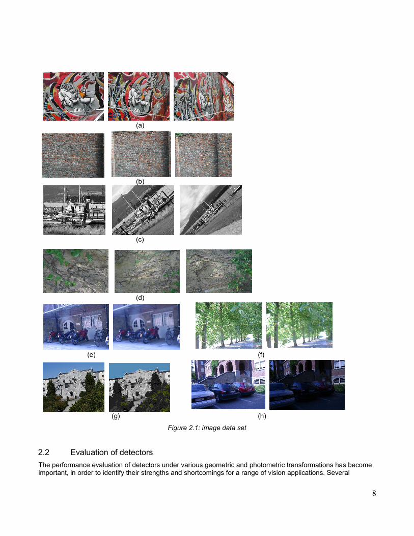
Figure 2.1 shows the image data set (proposed in [8]) used to evaluate the feature detectors and descriptors. Five different changes in imaging conditions are evaluated:
• View point changes: (a) and (b).
• Scale changes: (c) and (d).
• Image blur: (e) and (f).
• JPEG compression: (g).
• Illumination: (h).
In the cases of viewpoint change, scale change and blur, the same change in imaging conditions is applied to two different scene types:
• Structured scenes: contains homogeneous regions with distinctive edge boundaries (e.g., graffiti)
• Textured scenes: contains repeated textures of different forms.
7
(a)
(b)
(c)
(d)
(e) (f)
(g) (h)
Figure 2.1: image data set
2.2 Evaluation of detectors
The performance evaluation of detectors under various geometric and photometric transformations has become important, in order to identify their strengths and shortcomings for a range of vision applications. Several
8
approaches have been used for evaluating the performance of interest point detectors, including ground-truth verification, localization and theoretical analysis. However the most widely employed measure is the repeatabilityrate [2].
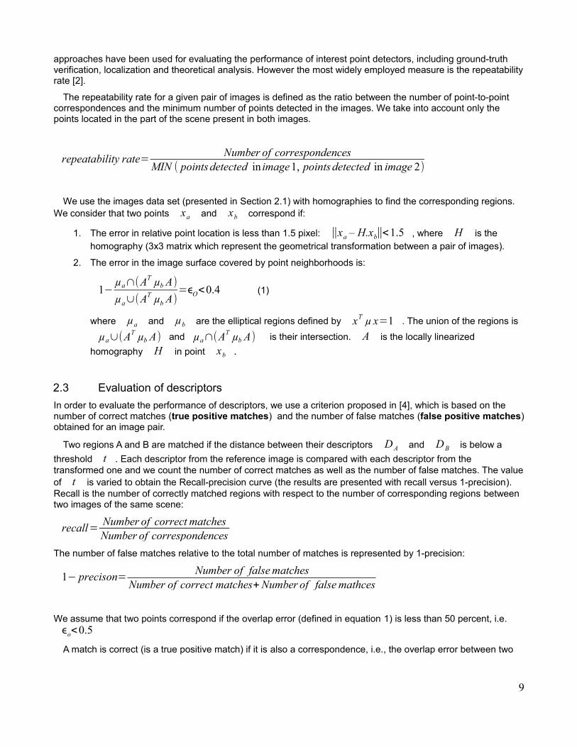
The repeatability rate for a given pair of images is defined as the ratio between the number of point-to-point correspondences and the minimum number of points detected in the images. We take into account only the points located in the part of the scene present in both images.
repeatability rate=Number of correspondences
MIN ( pointsdetected in image1, pointsdetected in image 2)
We use the images data set (presented in Section 2.1) with homographies to find the corresponding regions. We consider that two points xa and xb correspond if:
1. The error in relative point location is less than 1.5 pixel: ∥xa – H.xb∥<1.5 , where H is the homography (3x3 matrix which represent the geometrical transformation between a pair of images).
2. The error in the image surface covered by point neighborhoods is:
1−µa∩(AT µb A)
µa∪(AT µb A)=ϵO<0.4 (1)
where µa and µb are the elliptical regions defined by xT µ x=1 . The union of the regions is
µa∪(AT µb A) and µa∩(AT µb A) is their intersection. A is the locally linearized
homography H in point xb .
2.3 Evaluation of descriptors
In order to evaluate the performance of descriptors, we use a criterion proposed in [4], which is based on the number of correct matches (true positive matches) and the number of false matches (false positive matches)obtained for an image pair.
Two regions A and B are matched if the distance between their descriptors DA and DB is below a
threshold t . Each descriptor from the reference image is compared with each descriptor from the transformed one and we count the number of correct matches as well as the number of false matches. The valueof t is varied to obtain the Recall-precision curve (the results are presented with recall versus 1-precision). Recall is the number of correctly matched regions with respect to the number of corresponding regions between two images of the same scene:
recall=Number of correct matchesNumber of correspondences
The number of false matches relative to the total number of matches is represented by 1-precision:
1− precison=Number of falsematches
Number of correct matches+Number of false mathces
We assume that two points correspond if the overlap error (defined in equation 1) is less than 50 percent, i.e.ϵo<0.5
A match is correct (is a true positive match) if it is also a correspondence, i.e., the overlap error between two
9
regions A and B (represented by the descriptors DA and DB ) is less than 50 percent and the distance
between their descriptors is less than the threshold t
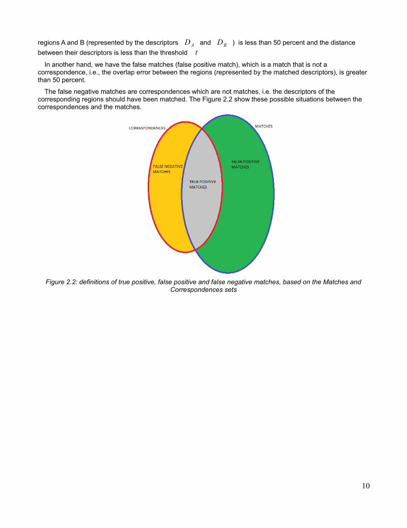
In another hand, we have the false matches (false positive match), which is a match that is not a correspondence, i.e., the overlap error between the regions (represented by the matched descriptors), is greater than 50 percent.
The false negative matches are correspondences which are not matches, i.e. the descriptors of the corresponding regions should have been matched. The Figure 2.2 show these possible situations between the correspondences and the matches.
Figure 2.2: definitions of true positive, false positive and false negative matches, based on the Matches andCorrespondences sets
10
Chapter 3
A framework for the performance evaluation ofdetectors and descriptors
Based on the metrics presented in chapter 2, an application to evaluate the performance of detectors and descriptors was developed. In this chapter we describe the design of this framework and the general structure of the OpenCV library, which is used to develop the framework.
3.1 The OpenCV library
OpenCV is an open source computer vision library available from http://SourceForge.net/projects/opencvlibrary. The library is written in C and C++ and runs under Linux, Windows and Mac OS X. OpenCV was designed for computational efficiency and with a strong focus on real-time applications. OpenCV is written in optimized C and can take advantage of multicore processors. One of the OpenCV's goals is to provide a simple-to-use computer vision infrastructure that helps people build fairly sophisticated vision applications quickly.
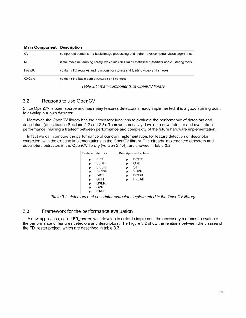
OpenCV is broadly structured into five main components, four of which are shown in Figure 3.1. The table 3.1 describes this main components [5].
CV component contains the basic image processing and higher-level computer vision algorithms.
ML is the machine learning library, which includes many statistical classifiers and clustering tools.
HighGUI contains I/O routines and functions for storing and loading video and images.
CXCore contains the basic data structures and content
Table 3.1: main components of OpenCV library
3.2 Reasons to use OpenCV
Since OpenCV is open source and has many features detectors already implemented, it is a good starting point to develop our own detector.
Moreover, the OpenCV library has the necessary functions to evaluate the performance of detectors and descriptors (described in Sections 2.2 and 2.3). Then we can easily develop a new detector and evaluate its performance, making a tradeoff between performance and complexity of the future hardware implementation.
In fact we can compare the performance of our own implementation, for feature detection or descriptor extraction, with the existing implementations in the OpenCV library. The already implemented detectors and descriptors extractor, in the OpenCV library (version 2.4.4), are showed in table 3.2:
Feature detectors Descriptor extractors
✔ SIFT✔ SURF✔ BRISK✔ DENSE✔ FAST✔ GFTT✔ MSER✔ ORB✔ STAR
✔ BRIEF✔ ORB✔ SIFT✔ SURF✔ BRISK✔ FREAK
Table 3.2: detectors and descriptor extractors implemented in the OpenCV library
3.3 Framework for the performance evaluation
A new application, called FD_tester, was develop in order to implement the necessary methods to evaluate the performance of features detectors and descriptors. The Figure 3.2 show the relations between the classes ofthe FD_tester project, which are described in table 3.3.
12
Figure 3.2: FD_tester class diagram
Class Description
Evaluator Implement the necessary functions to evaluate the performance of detectors and descriptors. In the version 1.0 of FD_Tester, the evaluation functions of the OpenCV library are used directly.Also, with this class is possible get the good matches (i.e. True positive matches) between a pair of images, based on the found correspondences and matches, in the performance evaluation funtions
DescriptorExtractorFactory This class know how to instantiate the available descriptor extractors
DetectorFactory This class know how to instantiate the available feature detectors classes.
DTO_Parameters Data Transfer Object (DTO) used for the parameters transmition through the user interface. The parameters are used to instantiate the detectors and descriptors extractor with a specific configuration.
DTO_detector_performance DTO used to transfer the information, respect to the performance of a detector, to the user interface
DTO_descriptorsPerformance DTO used to transfer the information, respect to the performance of a descriptor extractor, to the user interface.
Interface Implement the user interface
Table 3.3: FD_tester classes
13
Chapter 4
Software implementation of an Invariant feature detector
Although the final goal is to design a hardware architecture for invariant feature detection, it is very difficult to start directly with it. Then, instead of that, a software reference (called SIFT_SWA, because is a software approximation, based on the original SIFT algorithm proposed by D. Lowe in [1]) was developed, so that it is easy to make approximations in this one, without thinking in hardware implementation details, but having in mindsome constraints of the hardware implementation. Finally, when we are sure that SIFT_SWA has an acceptable performance, we can start with the hardware architecture design. To evaluate the performance of the new feature detector, we use FD_tester, described in Section 3.3.
4.1 Design
In order to keep the same interfaces, the class SIFT_SWA inherits the abstract class Feature2D (of the OpenCV library), implementing the detect and compute methods. The figure 4.1 show the relations between these classes.
The detect method implement the feature detection, and the compute method implement the descriptor extraction. Due to the Gaussian Pyramid and DoG pyramid structures are used to compute both features and descriptors, the functions to build these structures are shared for the detect and compute methods.
In our case, we just implement the detect method, and the compute method calls the compute method of the already implemented SIFT algorithm of the OpenCV library, but using the same Gaussian and DoG pyramids that use our detect method, which is helpful to see the impact in the descriptor extraction, of our approximated method used to build such structures.
Figure 4.1: relations between SIFT_SWA, SIFT and Feature2D
14
The Figure 4.2 shows the feature detection algorithm of SIFT_SWA.
Figure 4.2: SIFT_SWA algorithm
4.2 Gaussian filtering
The gaussian filtering consists on build a multiscale representation of the input image (the gaussian Pyramid), where each layer in the pyramid has an incremental smoothing regard the original image.
If we are searching keypoints on 2 scales (S = 2) of the input image, it is necessary 3 more scales, so that the Gaussian pyramid has S+3 layers, since they are used to build the Difference-of-Gaussian pyramid.
Based on the hardware implementation proposed in [7], we decide to make the Gaussian filtering with a direct approach, which reduce the hardware resource requirements, since it needs less memory resources than a cascade filtering approach.
Also we make separable convolution: the vertical convolution is followed by the horizontal convolution using 1D
15
gaussian kernels.
Since it is difficult to generate in hardware the 1D gaussian kernels, it is necessary to have a fixed NxM matrix ofinteger values, where N is the number of Gaussian kernels (S+3) and M is the maximal kernel size. If we use a kernel size of 5σ , the maximal kernel size is 33 ( σ corresponding to the most smoothing image in the gaussian pyramid). To get these integer values, the original gaussian coefficients (real values) are scaled by a factor multiple of two (e.g. 4096).
The smoothing factor ( σ ) of each layer in the Gaussian Pyramid is (Table 4.1):
Value
σ0 1.61
σ1 2.27
σ2 3.22
σ3 4.55
σ4 6.44
Table 4.1: Smoothing factor of each layer in the Gaussian Pyramid
4.3 Difference of gaussians
The difference-of-gaussians is computed subtracting each pair of pixel of neighboring smoothing images in the gaussian pyramid, getting a DoG pyramid with S+2 layers.
The Figure 4.3 show the Gaussian pyramid and DoG pyramid for the first and second octave.
Figure 4.3: Gaussian and DoG pyramids
4.4 Keypoint detection
The keypoint detection is divided in three steps:
• Extrema detection:
In order to detect the local maxima and minima, each sample point D( x , y ,σ) of the DoG pyramid is
16
compared to its eight neighbors in the current image and nine neighbors in the scale above and below (Figure 4.4). It is selected only if it is larger than all of these neighbors or smaller than all of them. The cost of this check is reasonably low due to the fact that most sample points will be eliminated following the first few checks.
Figure 4.4: Maxima and minima of the difference-of-Gaussian images are detected by comparing a pixel(marked with X) to its 26 neighbors in 3x3 regions at the current and adjacent scales (marked with circles)
• Keypoint location refinement: This processing step implies the extraction of 3D continuous extrema from the 3D discrete extrema (detected in the Extrema detection step). Since this processing step involves a high complexity for a hardware implementation, we decide to avoid it.
• Contrast check: If we avoid the keypoint location refinement step, the contrast check implies only a comparison with a threshold value.
• Edge responses elimination: like the Keypoint location refinement, the elimination implies a high complexity for hardware implementation, because it computes a Hessian matrix (which implies second order derivatives). However, based on the performance evaluation of SIFT_SWA (Figure 4.5), we can't avoid the edge response elimination, so that we propose for future work, to find an efficient method to eliminate edge responses.
Figure 4.5: descriptors performance evaluation, when the edge responses are eliminated or not.
4.5 Orientation assignment
We use the SIFT's method, of the OpenCV library, for the orientation assignment.
17
Chapter 5
Hardware implementation of an Invariant feature detector
5.1 A hardware architecture for extrema detection
In this section we make an overview of the hardware architecture proposed by Hamza, then for more implementation details, please see [7].
The figure 5.1 show the block diagram of the proposed hardware architecture for IFD2_HW.
Figure 5.1: Block diagram of the hardware architecture proposed in [7]
The number of input image lines required at a time is determined by the kernel size parameter which is set as the largest Gaussian kernel size to produce the most blurred scale. Also all the kernels are zero extended to make their size constant. The Block RAM based FIFO's are used for the input line buffers. The FIFO's are generated using the Xilinx Coregen utility.
Xilinx Coregen utility provides option to configure the width and depth of FIFO. In this case the width of image is 640 pixels of 8 bits each. Hence the depth of FIFO should be at least 640. Thus a possible option is to generate 16-bit wide and 1024 words deep FIFO's. However since one pixel only needs 8 bits, the other 8 bits remain free. To optimize this usage two image lines are concatenated in one such FIFO. The number of FIFO’s required are dependent on the kernel size. The kernel size is always odd and since in this design the current pixel is directly fed into the processing block, the number of lines that need to be buffered remain one less then the kernel size which is even and therefore the number of FIFO’s required becomes half of the kernel size less one.
The kernel coefficients are stored in a ROM. In this case five kernels are required to produce five scales. As a result the pixels for all five scales are computed with a gap of single cycle.
The next step is the difference of Gaussian to produce DoG scale space. Since the adjacent Gaussian scales are subtracted to get the DoG scales, the proposed architecture uses a single subtracter for all the scales with one additional register. The result from the DoG module is then saved in the Block RAM based buffers after a serial to parallel conversion module. Once the buffers get full the extrema detection module is activated. In the current implementation the extrema detection module only detects the maxima as the candidate keypoints.
18
Scale processing: The proposed architecture calculates different scales with the same hardware in a time multiplexed fashion. The input pixel is loaded into the line buffers after every s cycles, where s defines the number of Gaussian scales within one octave. At the initial stage when line buffer gets full, all the FIFO output lines contain valid data hence the first vertical window starts getting processed. The output of line buffers remain valid until these s clock cycles. In each cycle the pixels are convolved with the respective 1D Gaussian kernels. The result is buffered for the horizontal convolution.
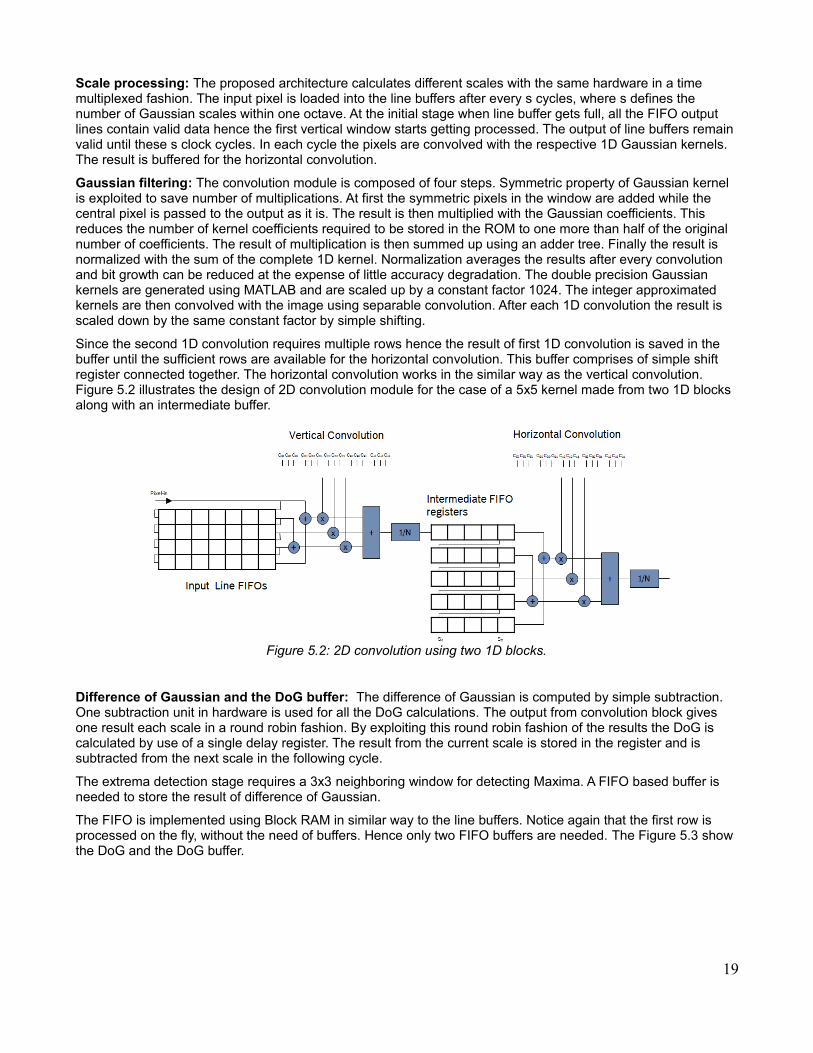
Gaussian filtering: The convolution module is composed of four steps. Symmetric property of Gaussian kernel is exploited to save number of multiplications. At first the symmetric pixels in the window are added while the central pixel is passed to the output as it is. The result is then multiplied with the Gaussian coefficients. This reduces the number of kernel coefficients required to be stored in the ROM to one more than half of the original number of coefficients. The result of multiplication is then summed up using an adder tree. Finally the result is normalized with the sum of the complete 1D kernel. Normalization averages the results after every convolution and bit growth can be reduced at the expense of little accuracy degradation. The double precision Gaussian kernels are generated using MATLAB and are scaled up by a constant factor 1024. The integer approximated kernels are then convolved with the image using separable convolution. After each 1D convolution the result is scaled down by the same constant factor by simple shifting.
Since the second 1D convolution requires multiple rows hence the result of first 1D convolution is saved in the buffer until the sufficient rows are available for the horizontal convolution. This buffer comprises of simple shift register connected together. The horizontal convolution works in the similar way as the vertical convolution. Figure 5.2 illustrates the design of 2D convolution module for the case of a 5x5 kernel made from two 1D blocks along with an intermediate buffer.
Figure 5.2: 2D convolution using two 1D blocks.
Difference of Gaussian and the DoG buffer: The difference of Gaussian is computed by simple subtraction. One subtraction unit in hardware is used for all the DoG calculations. The output from convolution block gives one result each scale in a round robin fashion. By exploiting this round robin fashion of the results the DoG is calculated by use of a single delay register. The result from the current scale is stored in the register and is subtracted from the next scale in the following cycle.
The extrema detection stage requires a 3x3 neighboring window for detecting Maxima. A FIFO based buffer is needed to store the result of difference of Gaussian.
The FIFO is implemented using Block RAM in similar way to the line buffers. Notice again that the first row is processed on the fly, without the need of buffers. Hence only two FIFO buffers are needed. The Figure 5.3 show the DoG and the DoG buffer.
19
Figure 5.3: DoG and Dog buffers
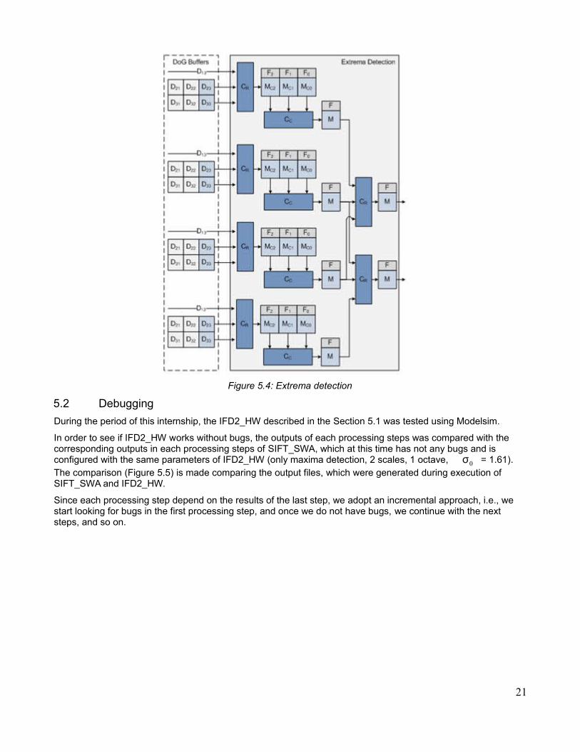
Extrema detection: The design of maxima detector is pipelined (Figure 5.4). The output from DoG buffer consists of three values that constitute one column of a 3x3 neighboring window. The DoG outputs a new column after every n clock cycles where n is the number of Gaussian scales. The extrema detection module hence runs on a lower clock, i.e. sysclk /n . In the first stage maxima is detected among the three elements of a column. The resulting maxima from each column are stored in pipeline registers. In addition a two bit register is used to keep track of the maxima location in the column. After the three consecutive columns have been processed, the next stage starts to detect maxima among these pipeline registers, in other words the row registers. The result is a maxima in a current 3x3 window for the single DoG scale. For every DoG scale a local maxima is detected in parallel. This adds to the number of comparators used which are directly proportional to the number of DoG scales.
20
Figure 5.4: Extrema detection
5.2 Debugging
During the period of this internship, the IFD2_HW described in the Section 5.1 was tested using Modelsim.
In order to see if IFD2_HW works without bugs, the outputs of each processing steps was compared with the corresponding outputs in each processing steps of SIFT_SWA, which at this time has not any bugs and is configured with the same parameters of IFD2_HW (only maxima detection, 2 scales, 1 octave, σ0 = 1.61). The comparison (Figure 5.5) is made comparing the output files, which were generated during execution of SIFT_SWA and IFD2_HW.
Since each processing step depend on the results of the last step, we adopt an incremental approach, i.e., we start looking for bugs in the first processing step, and once we do not have bugs, we continue with the next steps, and so on.
21
Figure 5.5: debugging IFD2_HW
In order to reduce the complexity of debugging, two testbenchs have been programmed:
• Reduced Testbench (Figure 5.6): only the IFD2_Main.vhd, which include all the modules concerning the IFD2_HW's algorithm, is tested receiving the parameters (input image start address, image width, image height, output start address) and the input image data (sramLoad1Sim.txt). The detected extremas are stored in an output file (sramDump1Sim.txt).
Figure 5.6: Reduced testbench
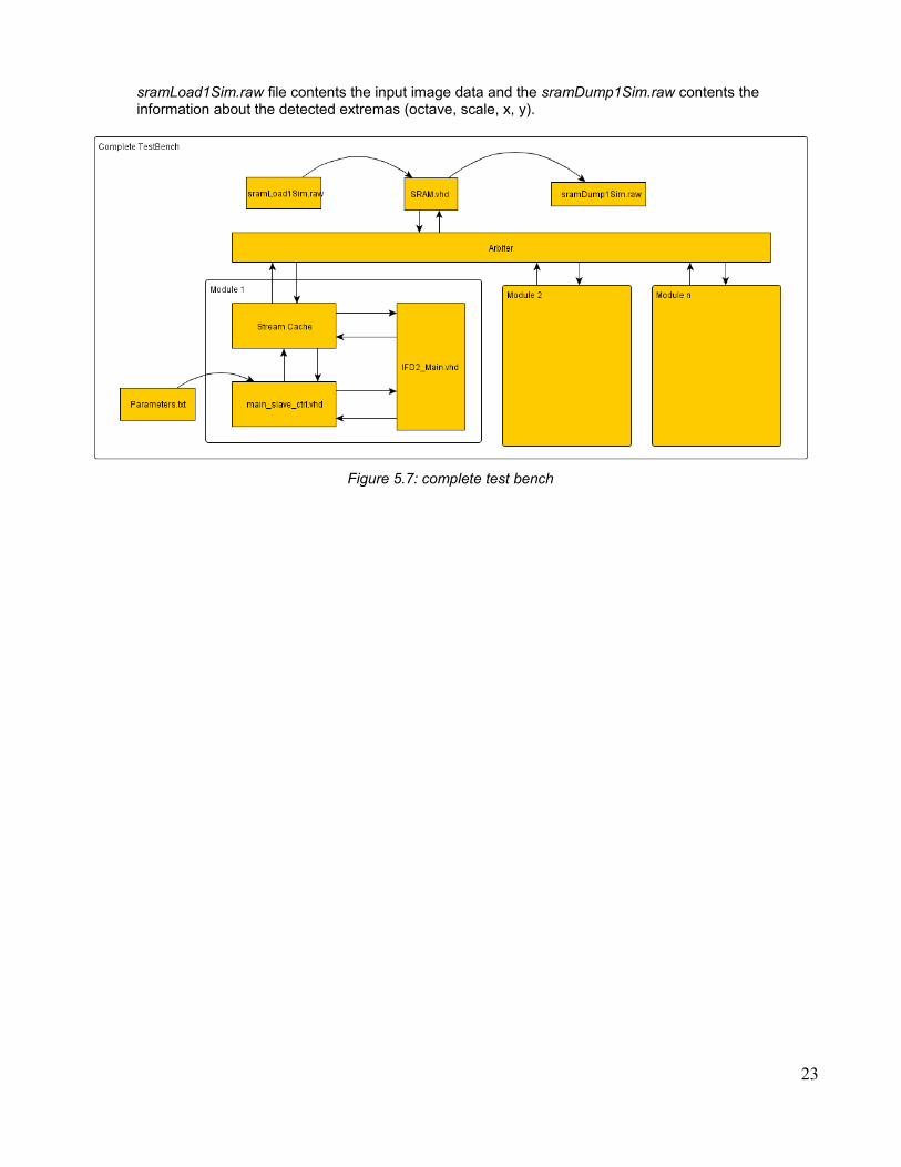
• Complete test bench (Figure 5.7): once the IFD2_Main module has been debugged, we can test the behavioral of such module with the rest of the system, i.e., the main slave controller and the Stream Cache. Also, in order to simulate the real environment, where the IFD2_HW will work, additional modules are added to the testbench, since the IFD2_HW must work together with the Orientation Assignment and Descriptors Extraction modules.
In this testbench the Modules 2 to n, actually just access to the SRAM memory, and the Arbiter must multiplex the PCI bus, which connect them with the SRAM memory. Thereby, when the PCI bus is busy by any of the Modules 2 to n the, the Stream Cache in the Module 1 will send the busy signal to the IFD2_Main module, and this should set the Data_enable signal with '0' in order to advice to the rest of the modules, into IFD2_Main, that there are not valid input data (stalling the pipelined architecture of IFD2_HW).
Initially the input image data are in the SRAM memory, the Stream cache read the pixel values of the input image from there, and send them to the IFD2_Main module. When IFD2_Main module finish the extrema detection, the information about the extremas are stored into the SRAM memory. The
22
sramLoad1Sim.raw file contents the input image data and the sramDump1Sim.raw contents the information about the detected extremas (octave, scale, x, y).
Figure 5.7: complete test bench
23
Found bugs
From the execution of the Reduced and complete testbench, the next bugs have been found (Table 5.1):
VHDL file Module Description Bugs Observations
fifo_1024x16.vhd FIFO used in Input Line and DoG Buffers
No
IFD2_Arith1.vhd Vertical convolution No
IFD2_Arith2.vhd Vertical convolution No
IFD2_Arith3.vhd Vertical convolution No
IFD2_Arith1_b.vhd Horizontal convolution No
IFD2_Arith2_b.vhd Horizontal convolution No
IFD2_Arith3_b.vhd Horizontal convolution No
IFD2_Conv_1D.vhd Vertical convolution No
IFD2_Conv_1D_b.vhd Horizontal convolution No
IFD2_Ctrl.vhd Controller yes Synchronization problem when the input line buffer is full
IFD2_DoG.vhd DoG (substracter and SIPO) No
IFD2_DoG_Main_Buff.vhd DoG Buffer yes The output values from DoG buffer are unordered.
IFD2_DoG_Sub_Buff.vhd DoG Buffer yes The output values from DoG buffer are unordered.
IFD2_Extrema_Detect.vhd Extrema detector yes
• Works only with unsigned values (the output of the difference of gaussians may be negative values).
• The counters, used to determine the extrema coordinates, have wrong values when an extrema is detected. Because when it is necessary advance to the next row (a new line is loaded in the DoG Buffer), these counters are not properly reset.
• The compators, used to determine if certain output value from the DoG buffer is a maxima, not always return a correct output.
IFD2_Half_Filt_Res_Buff.vhd Intermediate registers to store vertical convolution results
No
IFD2_Main.vhd Main No
IFD2_Norm.vhd Vertical convolution No
IFD2_Norm_b.vhd Horizontal convolution No
line_fifos_bram.vhd Input Line FiFOs No
ROM_coe.vhd Gaussian coefficients No
Table 5.1: Found bugs in the initial version of IFD2_HW
After the debugging, these bugs were fixed in both reduced and complete testbench. However, without bugs, theIFD2_HW need some improvements, in order to have better performance results. The Figure 5.8 show the detected extremas on the Graffiti image. This version of IFD_HW detect 57386 extremas (only maxima!). It is notpossible evaluate the performance of this version of IFD_HW due to the large number of detected extremas. Thereason of this huge number of detected keypoints may be because it is not making the contrast check, the edge responses elimination and is not enough accurate.
24
Figure 5.8: keypoints detected by the initial version of IFD2_HW
5.3 Improvements
Bit-width estimation
In order to improve the accuracy of the detector, it is necessary to estimate the bit-widths used to represent the values in each processing step of the detection. However we have to make a trade-off between hardware resource utilization and the accuracy.
We identify two main decisions, that affect the accuracy of the detector: Gaussian coefficients and Fixed-point representation of real values.
• Gaussian coefficient bit width: we must think on the number of necessary bits to represent each gaussian coefficient in hardware, which directly depend on the scaling factor used to get the integer
representation of such coefficients. Since the biggest coefficients are in the order of 10−2, the bit-
width is F−2 , where 2F is the scale factor used to convert the coefficients in integer values. In order to decide the best gaussian coefficient bit-width, we evaluate the detector performance and the effects in the descriptors performance due to the these different bit-widths (8, 10, 12, 13, 14, 15 and 16 bits) in SIFT_SWA (Figure 5.9):
25
(a) (b)
(c)
Figure 5.9: performance evaluation of SIFT_SWA, based on different bit-widths to represent the Gaussiancoefficients of the 1D kernels. (a) Repeatability, (b) Number of correspondences, (c) Recall-precision curve
We can see that, with 10 bits to represent the gaussian coefficients, we have an acceptable performance.
• Fixed-point: we have to decide the fractional part bit-width of the fixed-point values that will be used fromthe Gaussian filtering to the end of the detection algorithm. It is not necessary fixed-point to represent the input image pixels. But when SIFT_SWA do the vertical convolution, where it multiplies and adds the pixel values with the Gaussian coefficients (represented in fixed-point), is necessary to represent the smoothing images values in fixed-point, in order to increase the precision of the detection. Following the same approach to determine the bit-width, we evaluate the SIFT_SWA performance with different bit-widths to represent the fractional part of the fixed-point values of the smoothing images (Figure 5.10).
26
(a) (b)
(c)
Figure 5.10: performance evaluation of SIFT_SWA, based on different bit-widths to represent the fractional partof Fixed-point values. (a) Repeatability, (b) Number of correspondences, (c) Recall-precision curve
We can see that, with 7 bits to represent the fractional part of fixed-point values, we have an acceptable performance.
Based on this estimated bit-width, the Figure 5.11 show the bit-width configuration for each processing step of IFD2_HW.
27
Figure 5.11: bit-width configuration of IFD2_HW
Extrema detection:
Additionally to the maxima detection, minima detection is included, which consist just in add new comparators and registers like the maxima detection. Also, the contrast check is included in the same module (Extrema_Detect), which consist just in one comparison with the Contrast_threshold value. This module, with theDoG buffers, is shown in the Figure 5.12.
28
Figure 5.12: new extrema detector module of IFD2_HW
5.4 Comparison with the software reference
In order to compare the results between IFD2_HW and IFD2_SWA, it is used an image with a 192x144 resolution, reducing the execution time of the simulation in ModelSim. The Figure 5.13 shows the keypoints detected by both detectors.
29
(a) (b) (c)
Figure 5.13: (a) input image to the detectors, (b) detected keypoints by SIFT_SWA, (c) detected keypoints byIFD2_HW
These figures show that, SIFT_SWA and IFD2_HW get the same output (keypoints) for the same input image.
5.5 Synthesis
During the synthesis one problem in the hardware design of IFD2_HW was found: the maximum frequency of the whole system (i.e. the IFD2_Main module) is 75MHz. This is lower than the minimum frequency required for video real-time applications: 100MHz.
The reason of this problem was found in the last addition after the vertical and horizontal convolution (IFD2_Arith3 and IFD2_Arith3_b modules). Each of these modules add simultaneously 17 values, which limit themaximum possible frequency for both the vertical and horizontal convolution, due to the large delay produced by these modules. The problem is shown in Figure 5.14. However the maximum frequency of the whole system is only limited by the 17x1 adder in the vertical convolution.
Figure 5.14: 17x1 adder in horizontal and vertical convolution
To solve this problem, a pipelined addition of 3 stages was implemented (Figure 5.15 and 5.16)
30
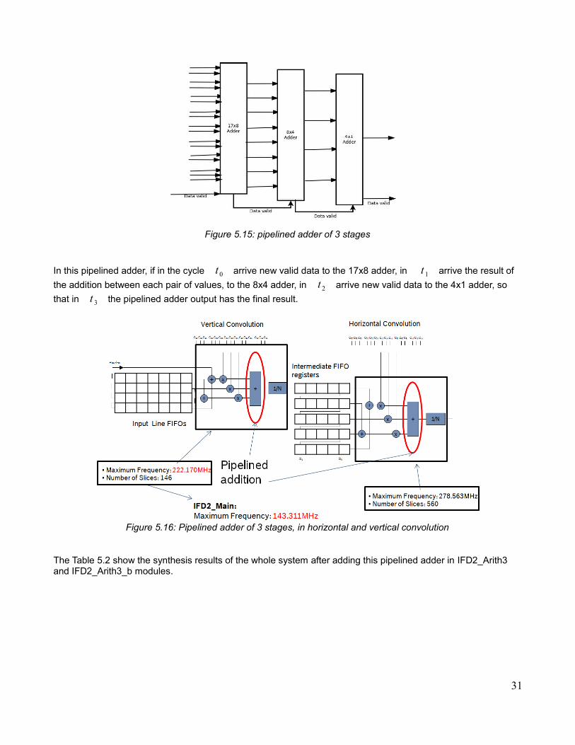
Figure 5.15: pipelined adder of 3 stages
In this pipelined adder, if in the cycle t 0 arrive new valid data to the 17x8 adder, in t 1 arrive the result of
the addition between each pair of values, to the 8x4 adder, in t 2 arrive new valid data to the 4x1 adder, so
that in t 3 the pipelined adder output has the final result.
Figure 5.16: Pipelined adder of 3 stages, in horizontal and vertical convolution
The Table 5.2 show the synthesis results of the whole system after adding this pipelined adder in IFD2_Arith3 and IFD2_Arith3_b modules.
31
IFD2_Main
Target Device xc4vfx60-12ff672
Implementation state Synthesis
Maximum Frequency 143.311MHz
Logic utilization Used Available Utilization
Number of slices 3399 25280 13%
Number of Slice Flip Flops 3865 50560 7%
Number of 4 input LUTs 4930 50560 9%
Number of bonded IOBs 211 352 59%
Number of FIFO16/RAMB16s
24 232 10%
Number of GCLKs 1 32 3%
Number of DSP 52 128 40%
Table 5.2: synthesis results of IFD2_HW
If we see the synthesis results with and without the pipelined addition, the hardware resource (Number of Slices)are not to much different. The reason of this, is that in each Slice there are some Flip-Flops (to implement registers) that we can use or not, but anyway these Slices are employed.
5.6 Additional improvements
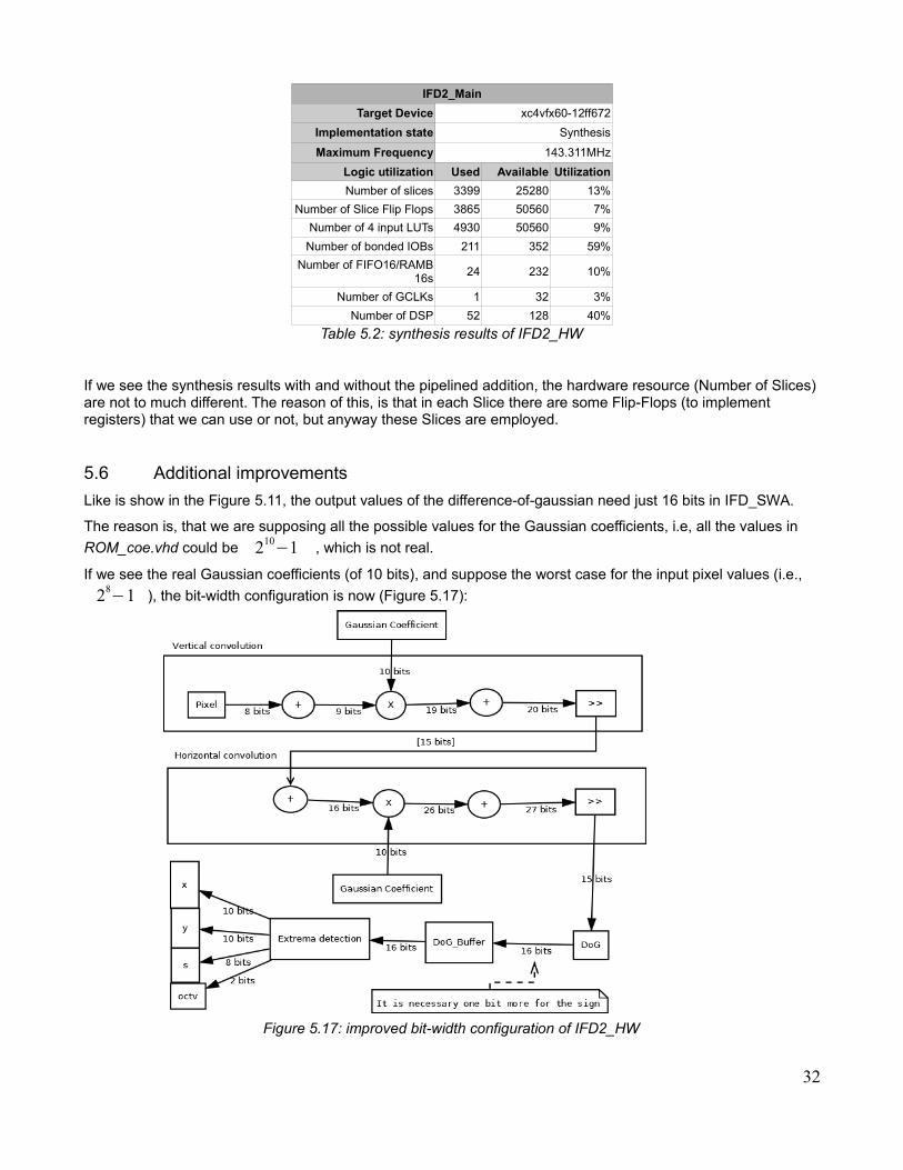
Like is show in the Figure 5.11, the output values of the difference-of-gaussian need just 16 bits in IFD_SWA.
The reason is, that we are supposing all the possible values for the Gaussian coefficients, i.e, all the values in
ROM_coe.vhd could be 210−1 , which is not real.
If we see the real Gaussian coefficients (of 10 bits), and suppose the worst case for the input pixel values (i.e.,
28−1 ), the bit-width configuration is now (Figure 5.17):
Figure 5.17: improved bit-width configuration of IFD2_HW
32
After this optimization in the bit-width, the synthesis results are like in the Table 5.3.
IFD2_Main
Target Device xc4vfx60-12ff672
Implementation state Synthesis
Maximum Frequency 160.235MHz
Logic utilization Used Available Utilization
Number of slices 2945 25280 11%
Number of Slice Flip Flops 3148 50560 6%
Number of 4 input LUTs 4418 50560 8%
Number of bonded IOBs 211 352 59%
Number of FIFO16/RAMB16s
24 232 10%
Number of GCLKs 1 32 3%
Number of DSP 35 128 27%
Table 5.3: synthesis results of the improved version of IFD2_HW
Finally the Figure 5.18 shows the performance results of this new version of IFD2_HW, in comparison with the original SIFT detector (implemented in the OpenCV library). The configuration of the detectors is similar, but the IFD2_HW is working only with 3 octaves (actually the software reference SIFT_SWA) and SIFT with 9 octaves. In SIFT_SWA, for the sub-sampling (in order to get each next octave), the original input image is employed.
Figure 5.18: performance results of SIFT and IFD2_HW with similar configuration
33
Like we can see in the these results, the repeatability and number of correspondences is higher in IFD2_HW than in SIFT, but the performance of the descriptors is really bad in IFD2_HW. Like was explained in Section 4.4,the reason of these bad descriptors, is that we are avoiding in IFD2_HW the edge elimination process, which can improves significantly the performance of the detector.
The Figure 5.19 compares the detected keypoints by SIFT and by IFD2_HW.
Although the synthesis results of the improved version of IFD2_HW are good enough, regard the maximum frequency and the required hardware resources, it is still necessary implement some modules, which improves the performance results of the detectors, e.g. the edge responses elimination modules.
On the other hand, still remains to implement the down-sampling module, in order to generate the initial image (from the original input image) for the next octaves. The best option would be 3 octaves, based on the performance results of SIFT_SWA. However, here we can choose between the separated processing of each octave (i.e. store the initial image for each octave in the external memory), which does not require any change inIFD2_HW, or it is possible process each octave at the same time, which requires to duplicate the hardware resources.
Finally, the IFD2_HW could require additional modifications in order to work together with the another implemented modules in hardware: Orientation Assignment and Descriptor Extraction modules. Also we have to see if the whole system (with these 3 modules) is still able to process each video frame in the required time (30 frames per second) on 640x180 images.
35
Bibliography
[1] David G. Lowe, Distinctive image features from scale-invariant keypoints, International Journal of Computer Vision, 60(2), 91-110 (2004).
[2] K. Mikolajczyk, C. Schmid, Scale & Affine Invariant Interest Point Detectors, International Journal of Computer Vision 60(1), 63–86 (2004).
[3] S. Ehsan, N. Kanwal, A.F. Clark and K.D. McDonald-Maier, Improved repeatability measures for evaluating performance of feature detectors, ELECTRONICS LETTERS Vol. 46 No. 14 (2010).
[4] K. Mikolajczyk, C. Schmid, A Performance Evaluation of Local Descriptors, IEEE TRANSACTIONS ON PATTERN ANALYSIS AND MACHINE INTELLIGENCE, VOL. 27, NO. 10 (2005).
[5] G. Bradski, A. Kaehler, Learning OpenCV, O'Reilly,(2008).
[6] The OpenCV Reference Manual, Release 2.4.4.0 (2013).
[7] B. I. Hamza, A Hardware Architecture for Scalespace Extrema Detection, Degree project in Communication Systems, Royal Institute of Technology, Stockholm, Sweden (2012).
[8] K. Mikolajczyk et. al., A Comparison of Affine Region Detectors, International Journal of Computer Vision (2006).
[9] D. Bailey, Design for Embedded Image Processing on FPGAs, John Wiley & Sons,(2011)