Internship report on the modelling of hydrogen peroxide to combat toxic algae blooms Name: Darryl Holsboer University: University of Amsterdam Internship host: Deltares Examiner: dr. Jolanda Verspagen Assessor: dr. Petra Visser Daily supervisor: dr. Anouk Blauw Advisors: dr. Miguel Dionisio Pires & dr. Tineke Troost Date: 13-01-2020
Cyanobacterial blooms are a growing problem worldwide due to their negative impact on
ecosystem functioning and water quality. Hydrogen peroxide (H2O2) has been implemented in the
last decade as a cost effective and environmentally friendly method, which may be used to
selectively kill cyanobacteria. In The Netherlands this method has been performed with varying
degrees of success. Thus, the main aim of this internship has been to develop a model that can
predict for a wide variety of field conditions the optimal application timing and dosage of hydrogen
peroxide in order to most effectively combat toxic cyanobacterial blooms. This model was developed
based on lab and field data provided by the University of Amsterdam. The lab data was used to set
up and calibrate the model, and the field data was used for validation. The degradation of hydrogen
peroxide (H2O2) and the decrease in photosynthetic yield (proxy for phytoplankton mortality) in dark
and light conditions were the primary modelled processes. Additionally, a sensitivity analysis was
performed with 10 scenarios based on important conditions such as: the target concentration H2O2,
the solar irradiance, turbidity, presence of eukaryotic phytoplankton, stratified or mixed water
columns and the delayed degradation of H2O2. Degradation of H2O2 and mortality of cyanobacteria
could be modelled relatively well in the lab. Field data proved to be more difficult to predict, as
many field conditions could not be considered. Still, the sensitivity analysis indicated that turbidity,
mixing depth, the presence of eukaryotic plankton and to a lesser degree the delay in H2O2
degradation determine the effectiveness of H2O2in this model. These results suggest that treatment
in early bloom stages would be most effective.
4
2. Description host institute
Deltares is an applied non-profit independent research institute active in the fields of subsurface,
infrastructure and water. It operates both nationally and internationally and is home to a wide range
of nationalities. Currently over 800 people are employed by Deltares; located in Delft and Utrecht.
The organization was established in 2008 as a merger of GeoDelft, Delft Hydraulics and parts of TNO
and the Dutch ministry of water and infrastructure.
Deltares aims to utilize the Dutch expertise on deltas and water management to develop innovative
and sustainable solutions for global problems related to water and soil. In the coming years Deltares
strives to become both nationally and internationally recognized as a ‘Triple A’ institute in these
domains (Deltares, 2018). The primary focus is on coastal areas, river catchments and deltas, since
these areas are increasingly being settled by people due to their economic potential. They are
however also very susceptible to the effects of climate change. Innovation and technology are key in
tackling these complex densely populated systems, which opens new opportunities for Deltares and
the Netherlands as a whole (Deltares, 2012).
The organisation is divided in six main units (Fig. 1). During the internship I was part of the unit
inland water systems. This unit can be further divided in six departments, of which I was part of the
Freshwater Ecology and Water Quality department (Fig. 1).
Figure 1: Deltares organisation chart
My activities were primarily related to the modelling in R of hydrogen peroxide effectiveness in
combatting toxic cyanobacterial blooms. Data fitting, model calibration, model validation and
sensitivity analysis were the most important steps undertaken.
I moreover did some additional literature research to fill in some knowledge gaps and I performed
data exploration and management in excel and Microsoft access on the datasets provided by the
University of Amsterdam and Dutch water boards. There were plans for a short lab experiment with
staining of cells using a flow cytometer to determine the actual mortality of cyanobacteria, but due
to time constraints it was decided to instead use the photosynthetic yield (Fv/Fm) as a proxy for the
5
mortality. Lastly, a report was written which is not only used to present my findings but also to
document how the model has been developed and what choices and assumptions were made.
3. Personal reflection
My internship was part of a collaboration between the University of Amsterdam and Deltares Delft
on the effectiveness of H2O2 in treating toxic cyanobacterial blooms.
I started this internship under the supervision of dr. Anouk Blauw with three main objectives. First, I
wanted to apply the theoretical knowledge that I had gathered over the years at the University of
Amsterdam. Second, I wanted to improve my programming skills and become more comfortable
using these skills. Third, I wanted to gain some valuable work experience.
During my internship I learned to be more independent, to cooperate and more importantly to ask
questions. Especially in the beginning I frequently discussed with the University of Amsterdam and
contacted other employees of Deltares for help when my daily supervisor was not available. While
there was a clear path I had to follow, I was free to provide my own input where necessary.
I moreover further improved upon my presentation skills, especially regarding the bi weekly
progress meetings, where I was required to keep my daily supervisor and advisors up to date. I also
attended a couple of department meetings where I presented my work to fellow department
colleagues.
In terms of programming I learned to create a simple numerical model from scratch in R studio,
which I had not done before. The programming courses I had followed at the University of
Amsterdam, which consisted mainly of Matlab with some R studio, fortunately proved to be enough
of a basis. The difference in programming language between Matlab and R studio did not pose too
much of a problem.
The hardest part of the internship as expected was to translate lab experiments to field situations.
Keeping the model simple, but not too simple was a key learning objective in this process. Working
with a limited amount of data and coming up with smart and efficient solutions was thus important.
On my own this would have been a difficult task, but with close collaboration with my daily
supervisor I managed to overcome or simplify most of the complexities in the model.
Ultimately, I learned a lot and I think I did achieve most of my objectives. I feel like I contributed to
Deltares by developing this model and I of course hope this model will be used and improved upon
in the future. I am moreover a lot more comfortable with my programming skills and would even
consider working in modelling related jobs. Joining the meetings also gave me more insight in the
inner workings of the company. I think working at Deltares showed me that there are many fields
where theoretical knowledge in earth sciences and environmental management may be applied.
6
4. Introduction
Toxic algae or cyanobacterial blooms are a common and increasing global problem occurring most
frequently in eutrophic ecosystems. The effects of these blooms can significantly impact ecosystem
services such as providing drinking water, recreation and agriculture (Lürling et al., 2014). Blooms
can negatively impact water quality by increasing turbidity and producing malodors; they can alter
ecosystems by causing anoxia and the subsequent death of other aquatic organisms. Cyanobacteria
also produce a wide range of toxins, of which microcystins are the most common (Lürling et al.,
2014). These toxins can badly affect the nervous, dermal, digestive, endocrine and hepatopancreatic
systems in humans and mammals (Paerl, 2014).
Cyanobacteria have adapted to a wide range of conditions and environments because of their
extensive evolutionary history (Paerl, 2014). This evolutionary genetic diversity has permitted
cyanobacteria to outcompete other phytoplankton species under eutrophic conditions.
This is because some cyanobacteria can fixate atmospheric nitrogen and are thus able to grow in
nitrogen limited environments, moreover in presence of elevated levels of phosphate and iron
bloom development can occur (Huisman et al., 2018).
Cyanobacteria are buoyant and can float to the surface, due to hollow gas filled cell compartments
called gas vesicles. Floating cyanobacteria can block light from reaching the lower depths, thereby
stifling the growth of competing less harmful eukaryotic phytoplankton. Some species can even
migrate up and down the water column such as the Planktothrix rubescens enabling a wider
potential area where nutrients may be exploited (Huisman et al., 2018).
Cyanobacterial toxins may act as prevention against grazing and may help with reducing oxidative
stress by binding on cyanobacteria specific proteins and enzymes (Huisman et al., 2018).
Multiple methods to combat toxic algae blooms are available and have been successful in
combatting cyanobacteria such as: copper sulfate (Van Hullebusch et al., 2002), flock and lock (de
Magalhães et al., 2017; Waajen et al., 2016), ultrasonication (Ahn et al., 2007), flushing and artificial
mixing (Visser et al., 1996; Verspagen et al., 2006). However, most of these are either expensive,
environmentally unfriendly or do not degrade cyanotoxins (Matthijs et al., 2016, Weenink et al.,
2015; Barrington et al., 2015). Hydrogen peroxide is a possible solution that could help with these
negative effects, since it is relatively inexpensive, degrades into water and oxygen in a couple of
days, selectively kills cyanobacteria by targeting the photosystems and could even help reduce
released concentrations of cyanotoxins (Barrington et al., 2015; Mikula et al., 2012).
In the Netherlands, experimentation with H2O2 in the field started in 2009 (Matthijs et al., 2012). In
this initial experiment a 2mg/l H2O2 successfully reduced cyanobacteria concentrations by 99%
within the first couple of days with minimal effects on remaining aquatic organisms. A similar decline
was visible for cyanotoxins, but with a 2-day lag. Whether a treatment succeeds or fails is very
dependent on specific field conditions. Since this initial experiment H2O2 has been applied over the
years to varying degrees of success.
In order to improve the success rate of treatments and to better understand the underlying
mechanisms a model has been developed in order to predict for a range of field conditions the
optimal application timing and dosage of hydrogen peroxide in order to most effectively combat
toxic algae blooms. For the field conditions the following parameters were considered: cloudiness,
7
turbidity, concentration H2O2, time of H2O2 degradation and the composition cyanobacteria and
eukaryotic phytoplankton.
5. Theoretical framework
5.1. H2O2 as a selective algicide
H2O2 can be applied as a selective measure to combat cyanobacterial blooms. This is because in
contrast to eukaryotic phytoplankton species, cyanobacteria utilize different reactions during
photosynthesis. The eukaryotic phytoplankton species use the Mehler-reaction which produces
H2O2. This toxic chemical is thereafter neutralized by catalase and peroxidase enzymes. In
cyanobacteria this reaction is replaced with a Mehler-like reaction. The key difference is the absence
of H2O2 production during photosynthesis, instead H2O is produced by Flavodiiron proteins
(Allahverdiyeva et al., 2014). Because there is no H2O2 produced it is believed that cyanobacteria
have a lower natural defense to H2O2. This is also supported by Weenink et al. (2015), according to
whom cyanobacteria have less enzymes that neutralize H2O2 than eukaryotic phytoplankton species.
5.2. Toxic versus nontoxic strains
Cyanobacteria have some defense mechanism against H2O2, though the effectiveness differs
between species and strains of cyanobacteria. According to a study by Schuurmans et al. (2018),
cyanobacteria that produce microcystins may be more vulnerable to H2O2 than other species of
cyanobacteria depending on the H2O2 concentration. Under natural conditions (1 – 50 µgram H2O2/l)
toxic strains of cyanobacteria appear to be better protected against H2O2. During treatments
however these concentrations are much greater and can reach as high as 120 mg/l in some specific
cases (Huo et al., 2015). At these concentrations H2O2 becomes toxic to more than just
cyanobacteria, however even at slightly elevated concentrations in the order of two to three times
the natural level, toxic strains lose their advantage to non-toxic strains, who appear to be better
protected to oxidative stress (Schuurmans et al., 2018). It is thus far unknown if this holds true for
other species of cyanobacteria, since there are many possible mechanisms that cyanobacteria utilize
to manage oxidative stress (Schuurmans et al., 2018).
5.3. H2O2 effectiveness
The degradation rate of hydrogen peroxide (H2O2) is dependent on the available oxidizable
compounds. In a study conducted by Tao et al., (2009) cellular respiration and enzymatic
degradation of H2O2 was compared with and without added glucose. Without glucose measured O2
concentrations decreased slowly and did not increase after addition of catalase. With glucose
measured O2 decreased faster, but also increased after catalase was added. This is because catalase
is an enzyme that catalyzes the degradation of H2O2 into H2O and O2. With glucose more O2 is
produced than is consumed, which indicates that more H2O2 is degraded when more glucose is
available.
8
Light intensity does not appear to alter the rate of H2O2 degradation in lab conditions (Piel et al.,
unpublished). However, light intensity in combination with application of H2O2 is suggested to
strongly influence the reduction of Fv/Fm in cyanobacteria. Fv/Fm is the ratio between variable
fluorescence of chlorophyll and minimum fluorescence of chlorophyll and is a widely used ratio to
measure stress in plants and cyanobacteria (Matthijs et al., 2012). It is hypothesized that a higher
light intensity leads to the generation of more oxygen radicals due to the photo fenton reaction
(Ruppert et al., 1993; Piel et al, unpublished). This in turn can inflict more damage on the
photosystems of cyanobacteria. Depending on the concentration H2O2 and light intensity this could
imply an order of magnitude greater decrease of Fv/Fm under light conditions compared to dark
conditions (Drábková et al., 2007).
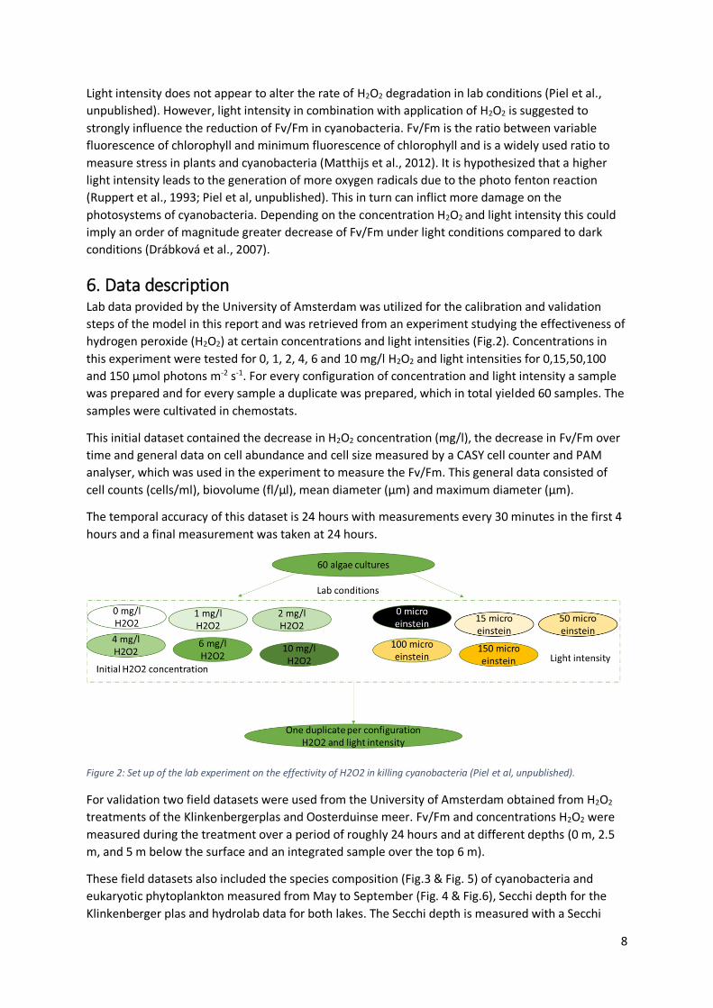
6. Data description Lab data provided by the University of Amsterdam was utilized for the calibration and validation
steps of the model in this report and was retrieved from an experiment studying the effectiveness of
hydrogen peroxide (H2O2) at certain concentrations and light intensities (Fig.2). Concentrations in
this experiment were tested for 0, 1, 2, 4, 6 and 10 mg/l H2O2 and light intensities for 0,15,50,100
and 150 µmol photons m-2 s-1. For every configuration of concentration and light intensity a sample
was prepared and for every sample a duplicate was prepared, which in total yielded 60 samples. The
samples were cultivated in chemostats.
This initial dataset contained the decrease in H2O2 concentration (mg/l), the decrease in Fv/Fm over
time and general data on cell abundance and cell size measured by a CASY cell counter and PAM
analyser, which was used in the experiment to measure the Fv/Fm. This general data consisted of
cell counts (cells/ml), biovolume (fl/µl), mean diameter (µm) and maximum diameter (µm).
The temporal accuracy of this dataset is 24 hours with measurements every 30 minutes in the first 4
hours and a final measurement was taken at 24 hours.
Figure 2: Set up of the lab experiment on the effectivity of H2O2 in killing cyanobacteria (Piel et al, unpublished).
For validation two field datasets were used from the University of Amsterdam obtained from H2O2
treatments of the Klinkenbergerplas and Oosterduinse meer. Fv/Fm and concentrations H2O2 were
measured during the treatment over a period of roughly 24 hours and at different depths (0 m, 2.5
m, and 5 m below the surface and an integrated sample over the top 6 m).
These field datasets also included the species composition (Fig.3 & Fig. 5) of cyanobacteria and
eukaryotic phytoplankton measured from May to September (Fig. 4 & Fig.6), Secchi depth for the
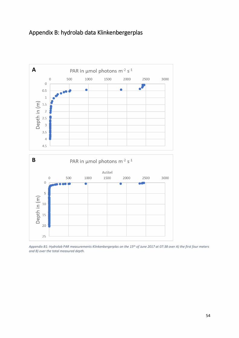
Klinkenberger plas and hydrolab data for both lakes. The Secchi depth is measured with a Secchi
9
disk. The depth at which the Secchi disk loses its visibility is used as a measure of transparency
(Preisendorfer, 1986). The hydrolab is a multiparameter probe used for measuring water quality.
Secchi depth and hydrolab measurements were measured for the months May to August. The
hydrolab measured: depth, temperature, salinity, photosynthetically active radiation (PAR),
chlorophyll fluorescence (in volt), dissolved oxygen and specific conductance over nearly the entire
depth of both lakes.
Additionally, a monitoring dataset with chemical and physical properties of Dutch water bodies was
available from Dutch water boards, however this dataset was not used in the development of this
model.
Klinkenberger plas
Figure 3: Dynamics in biovolume of cyanobacteria and eukaryotic phytoplankton in Klinkenberger Plas from June 15 2017 to June 18 2017.
10
Figure 4: Physical parameters in Klinkenberger Plas on June 15 2017. Depth profiles of (a) the density of water and (b) chlorophyll fluorescence at 7:38 in the morning.
The density was calculated only from temperature, since no salinity was measured in this lake
(Appendix B2 & B3) with the following simplified equation Eq. (1):
𝜌(𝑇) = 𝜌 × (1 − 𝛾(𝑇 − 4°𝐶)2) + 𝑆 (Eq. 1)
B
A
11
Where 𝜌 = density (1000 kg m-3)
𝑇 = temperature in ° C
𝛾 = temperature dependent change in density (6.493 x 10⁻⁶ K-1)
𝑆 = salinity in (g/l)
In the hydrolab and species composition data of the Klinkenbergerplas (Fig. 3 & Fig. 4) three main
observations could be made. First, the concentrations of cyanobacteria appeared to be much greater
than the concentrations of eukaryotic phytoplankton. Roughly 99% of the measured phytoplankton
consisted of cyanobacteria. Second, in the upper 2m the density was relatively constant, suggesting
the presence of a mixed layer depth. Third, two chlorophyll peaks could be observed in the data at a
depth of around 2m and 5m below the surface.
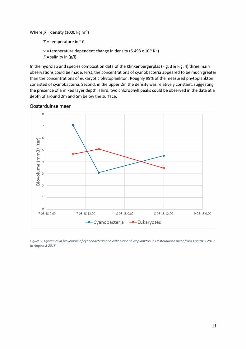
Oosterduinse meer
Figure 5: Dynamics in biovolume of cyanobacteria and eukaryotic phytoplankton in Oosterduinse meer from August 7 2018 to August 8 2018.
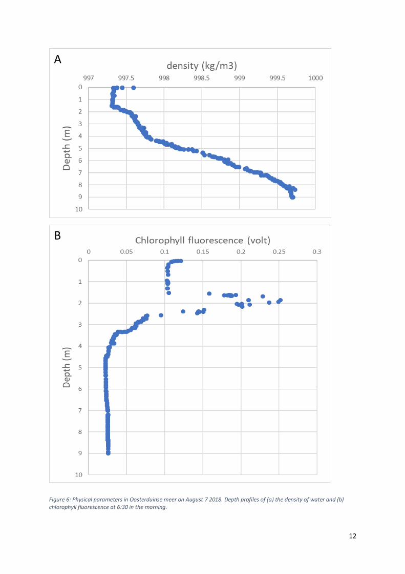
12
Figure 6: Physical parameters in Oosterduinse meer on August 7 2018. Depth profiles of (a) the density of water and (b) chlorophyll fluorescence at 6:30 in the morning.
A
B
13
In the hydrolab and species composition data for the Oosterduinse meer the conditions were
different compared to the Klinkenbergplas (Fig.5 & Fig.6). One reason was because of the increased
presence of eukaryotes, which for the Oosterduinse meer made up roughly 40% of the total
concentration phytoplankton.
Furthermore, only one chlorophyll peak was present at around 1.8 m below the surface. A similarity
with the dataset of the Klinkenberger plas could also be observed, since the pycnocline, the point at
which the density changes, appeared to be located at roughly the same depth (1.6m). The key
difference being that this change in density appears to be related to salinity as opposed to
temperature (Appendix C2 & C3).
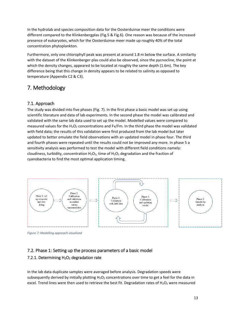
7. Methodology
7.1. Approach The study was divided into five phases (Fig. 7). In the first phase a basic model was set up using
scientific literature and data of lab experiments. In the second phase the model was calibrated and
validated with the same lab data used to set up the model. Modelled values were compared to
measured values for the H2O2 concentrations and Fv/Fm. In the third phase the model was validated
with field data; the results of this validation were first produced from the lab model but later
updated to better emulate the field observations with an updated model in phase four. The third
and fourth phases were repeated until the results could not be improved any more. In phase 5 a
sensitivity analysis was performed to test the model with different field conditions namely:
cloudiness, turbidity, concentration H2O2, time of H2O2 degradation and the fraction of
cyanobacteria to find the most optimal application timing.
Figure 7: Modelling approach visualized
7.2. Phase 1: Setting up the process parameters of a basic model
7.2.1. Determining H2O2 degradation rate
In the lab data duplicate samples were averaged before analysis. Degradation speeds were
subsequently derived by initially plotting H2O2 concentrations over time to get a feel for the data in
excel. Trend lines were then used to retrieve the best fit. Degradation rates of H2O2 were measured
14
in the presence and absence of cyanobacteria in the lab. This model used the degradation rate of
H2O2 in the presence of cyanobacteria.
For the time series a time period of 24 hours was taken with a timestep of 0.1 hours (6min) and for
data fitting an exponential model was deemed to be the best model to describe the process. This is
also in accordance with results from Richard et al. (2007). From the underlying equation the
degradation rate was derived.
In R studio Version 1.2.1335, the data was subsequently plotted and fitted with an exponential
model similarly to excel (Eq. 1). This was performed with a custom exponential function and the
standard NLS function from the stats package in R. The “NLS” function used the custom exponential
function as an input and calculated the nonlinear (weighted) least- squares estimates, which was
thereafter used to retrieve a best fit by using the “coef” function. With the curve function the best fit
could then be visualized in a plot.
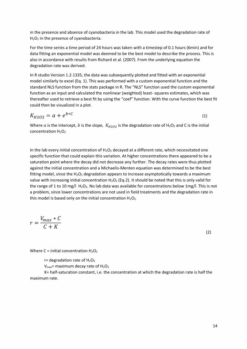
𝐾𝐻2𝑂2 = 𝑎 + 𝑒𝑏∗𝐶 (1)
Where 𝑎 is the intercept, 𝑏 is the slope, 𝐾𝐻2𝑂2 is the degradation rate of H2O2 and C is the initial
concentration H2O2
In the lab every initial concentration of H2O2 decayed at a different rate, which necessitated one
specific function that could explain this variation. At higher concentrations there appeared to be a
saturation point where the decay did not decrease any further. The decay rates were thus plotted
against the initial concentration and a Michaelis-Menten equation was determined to be the best
fitting model, since the H2O2 degradation appears to increase asymptotically towards a maximum
value with increasing initial concentration H2O2 (Eq.2). It should be noted that this is only valid for
the range of 1 to 10 mg/l H2O2. No lab data was available for concentrations below 1mg/l. This is not
a problem, since lower concentrations are not used in field treatments and the degradation rate in
this model is based only on the initial concentration H2O2.
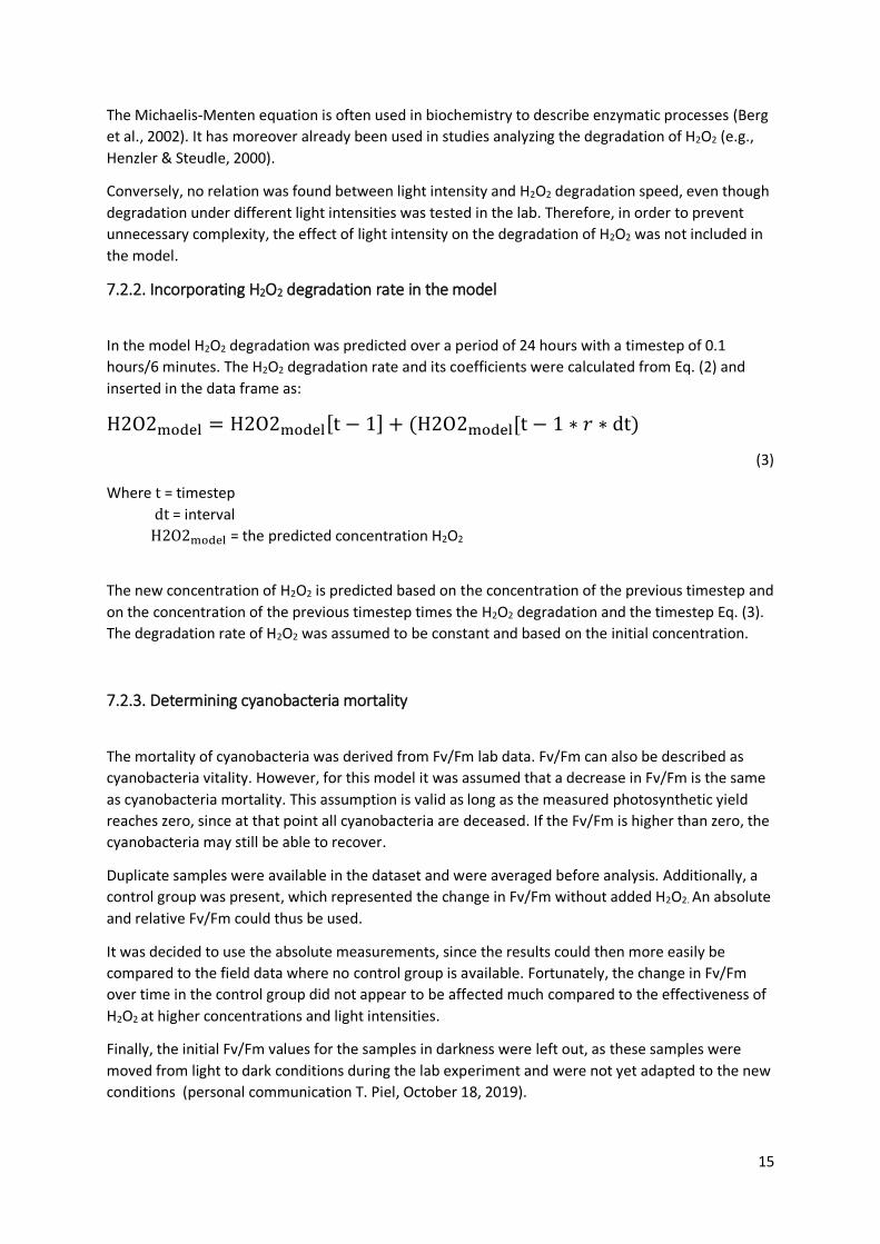
𝑟 =𝑉𝑚𝑎𝑥 ∗ 𝐶
𝐶 + 𝐾
(2)
Where C = initial concentration H2O2
r= degradation rate of H2O2
Vmax= maximum decay rate of H2O2
K= half-saturation constant, i.e. the concentration at which the degradation rate is half the
maximum rate.
15
The Michaelis-Menten equation is often used in biochemistry to describe enzymatic processes (Berg
et al., 2002). It has moreover already been used in studies analyzing the degradation of H2O2 (e.g.,
Henzler & Steudle, 2000).
Conversely, no relation was found between light intensity and H2O2 degradation speed, even though
degradation under different light intensities was tested in the lab. Therefore, in order to prevent
unnecessary complexity, the effect of light intensity on the degradation of H2O2 was not included in
the model.
7.2.2. Incorporating H2O2 degradation rate in the model
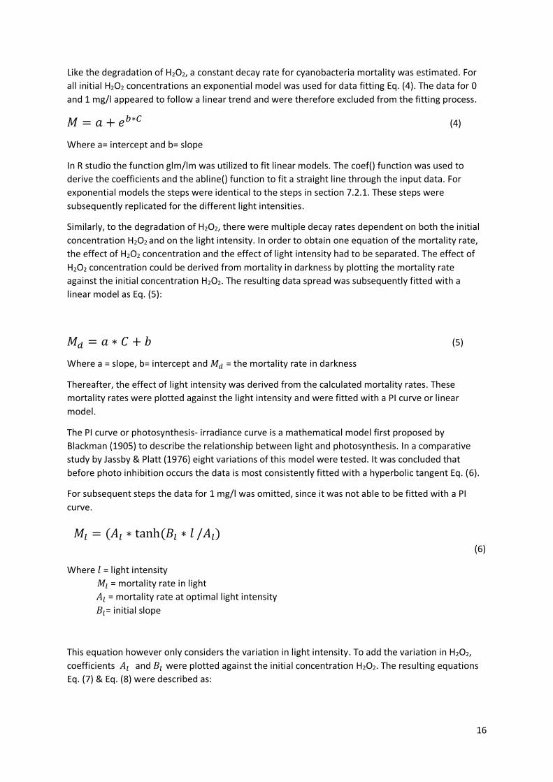
In the model H2O2 degradation was predicted over a period of 24 hours with a timestep of 0.1
hours/6 minutes. The H2O2 degradation rate and its coefficients were calculated from Eq. (2) and
The new concentration of H2O2 is predicted based on the concentration of the previous timestep and
on the concentration of the previous timestep times the H2O2 degradation and the timestep Eq. (3).
The degradation rate of H2O2 was assumed to be constant and based on the initial concentration.
7.2.3. Determining cyanobacteria mortality
The mortality of cyanobacteria was derived from Fv/Fm lab data. Fv/Fm can also be described as
cyanobacteria vitality. However, for this model it was assumed that a decrease in Fv/Fm is the same
as cyanobacteria mortality. This assumption is valid as long as the measured photosynthetic yield
reaches zero, since at that point all cyanobacteria are deceased. If the Fv/Fm is higher than zero, the
cyanobacteria may still be able to recover.
Duplicate samples were available in the dataset and were averaged before analysis. Additionally, a
control group was present, which represented the change in Fv/Fm without added H2O2. An absolute
and relative Fv/Fm could thus be used.
It was decided to use the absolute measurements, since the results could then more easily be
compared to the field data where no control group is available. Fortunately, the change in Fv/Fm
over time in the control group did not appear to be affected much compared to the effectiveness of
H2O2 at higher concentrations and light intensities.
Finally, the initial Fv/Fm values for the samples in darkness were left out, as these samples were
moved from light to dark conditions during the lab experiment and were not yet adapted to the new
conditions (personal communication T. Piel, October 18, 2019).
16
Like the degradation of H2O2, a constant decay rate for cyanobacteria mortality was estimated. For
all initial H2O2 concentrations an exponential model was used for data fitting Eq. (4). The data for 0
and 1 mg/l appeared to follow a linear trend and were therefore excluded from the fitting process.
𝑀 = 𝑎 + 𝑒𝑏∗𝐶 (4)
Where a= intercept and b= slope
In R studio the function glm/lm was utilized to fit linear models. The coef() function was used to
derive the coefficients and the abline() function to fit a straight line through the input data. For
exponential models the steps were identical to the steps in section 7.2.1. These steps were
subsequently replicated for the different light intensities.
Similarly, to the degradation of H2O2, there were multiple decay rates dependent on both the initial
concentration H2O2 and on the light intensity. In order to obtain one equation of the mortality rate,
the effect of H2O2 concentration and the effect of light intensity had to be separated. The effect of
H2O2 concentration could be derived from mortality in darkness by plotting the mortality rate
against the initial concentration H2O2. The resulting data spread was subsequently fitted with a
linear model as Eq. (5):
𝑀𝑑 = 𝑎 ∗ 𝐶 + 𝑏 (5)
Where a = slope, b= intercept and 𝑀𝑑 = the mortality rate in darkness
Thereafter, the effect of light intensity was derived from the calculated mortality rates. These
mortality rates were plotted against the light intensity and were fitted with a PI curve or linear
model.
The PI curve or photosynthesis- irradiance curve is a mathematical model first proposed by
Blackman (1905) to describe the relationship between light and photosynthesis. In a comparative
study by Jassby & Platt (1976) eight variations of this model were tested. It was concluded that
before photo inhibition occurs the data is most consistently fitted with a hyperbolic tangent Eq. (6).
For subsequent steps the data for 1 mg/l was omitted, since it was not able to be fitted with a PI
curve.
(6)
Where 𝑙 = light intensity
𝑀𝑙 = mortality rate in light
𝐴𝑙 = mortality rate at optimal light intensity
𝐵𝑙= initial slope
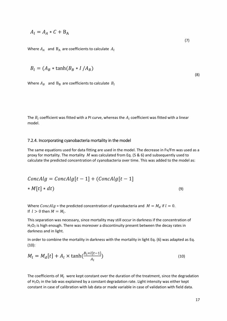
This equation however only considers the variation in light intensity. To add the variation in H2O2,
coefficients 𝐴𝑙 and 𝐵𝑙 were plotted against the initial concentration H2O2. The resulting equations
Eq. (7) & Eq. (8) were described as:
𝑀𝑙 = (𝐴𝑙 ∗ tanh(𝐵𝑙 ∗ 𝑙 /𝐴𝑙)
17
(7)
Where 𝐴𝐴 and BA are coefficients to calculate 𝐴𝑙
(8)
Where 𝐴𝐵 and BB are coefficients to calculate 𝐵𝑙
The 𝐵𝑙 coefficient was fitted with a PI curve, whereas the 𝐴𝑙 coefficient was fitted with a linear
model.
7.2.4. Incorporating cyanobacteria mortality in the model
The same equations used for data fitting are used in the model. The decrease in Fv/Fm was used as a proxy for mortality. The mortality 𝑀 was calculated from Eq. (5 & 6) and subsequently used to calculate the predicted concentration of cyanobacteria over time. This was added to the model as:
𝐶𝑜𝑛𝑐𝐴𝑙𝑔 = 𝐶𝑜𝑛𝑐𝐴𝑙𝑔[𝑡 − 1] + (𝐶𝑜𝑛𝑐𝐴𝑙𝑔[𝑡 − 1]
∗ 𝑀[𝑡] ∗ 𝑑𝑡) (9)
Where 𝐶𝑜𝑛𝑐𝐴𝑙𝑔 = the predicted concentration of cyanobacteria and 𝑀 = 𝑀𝑑 if 𝑙 = 0.
If 𝑙 > 0 then 𝑀 = 𝑀𝑙.
This separation was necessary, since mortality may still occur in darkness if the concentration of
H2O2 is high enough. There was moreover a discontinuity present between the decay rates in
darkness and in light.
In order to combine the mortality in darkness with the mortality in light Eq. (6) was adapted as Eq.
(10):
𝑀𝑙 = 𝑀𝑑[𝑡] + 𝐴𝑙 × tanh(𝐵𝑙×𝑙[𝑡−1]
𝐴𝑙) (10)
The coefficients of 𝑀𝑙 were kept constant over the duration of the treatment, since the degradation
of H2O2 in the lab was explained by a constant degradation rate. Light intensity was either kept
constant in case of calibration with lab data or made variable in case of validation with field data.
𝐴𝑙 = 𝐴𝐴 ∗ 𝐶 + BA
𝐵𝑙 = (𝐴𝐵 ∗ tanh(𝐵𝐵 ∗ 𝐼 /𝐴𝐵)
18
7.3. Phase 2: Validation of the lab model
Validation of the model was performed by plotting measured concentrations of H2O2 and Fv/Fm,
against the modelled concentrations of H2O2 and Fv/Fm.
7.4. Phase 3: Implementing modifications for a field model
The model was initially calibrated with lab data. However, in the lab the light intensity was constant,
while in the field light intensity was variable over time and over depth. Three things were required
to determine light intensity in the field. 1) The law of Lambert-Beer, which was applied to determine
light intensity over depth for one specific point in time. 2) In order to capture the variation in
irradiance throughout the day measurements of the Royal Netherlands Meteorological institute
(KNMI) were used. 3) The light extinction coefficient, which is used in the Lambert-Beer equation,
was derived from hydrolab data.
7.4.1. Calculating light intensity over depth in the field using two light models
Validation of the model was performed with two datasets from the Oosterduinse meer and the
Klinkenbergerplas. In order to better simulate light conditions in the field two light models were
implemented for this purpose according to the law of Lambert-Beer: a model to calculate light
intensity at depth Z Eq. (11), which was used for stratified lakes and a model to calculate light
intensity over the mixed layer depth Zm Eq. (12), which was used for lakes with mixed layers. These
models can be described as:
𝐼𝑧 = 𝐼0𝑒−𝐾𝑑𝑍 (11)
𝐼𝑚 = 𝐼0(1 − 𝑒−𝐾𝑑𝑍𝑚) (12)
Where Iz is the irradiance (in μmol photons m-2 s-1) at depth Z (in m), Im is the irradiance at mixed
layer depth Zm, I0 is the solar irradiance at the surface, Kd is the light extinction coefficient (in m-1).
These two models were used so a distinction could be made between stratified lakes and lakes
where mixing occurred.
7.4.2. Implementing daily variation in solar irradiance
19
Hourly measurements of the solar irradiance (in J cm-2 h-1) from the weather stations of Voorschoten
and Schiphol were used as the input for the irradiance at the water surface. Since, cyanobacteria do
not utilize the entire solar spectrum a correction factor of 0.45 was used to convert sunlight to PAR.
This factor approximates the fraction PAR of the total solar irradiance (Kirk, 1994). Thereafter, J cm-2
h-1 was converted to μmol photons m-2 s-1, using Avogadro’s constant and with the assumption that
one Joule equals 2.77 x 10¹⁸ photons (Kirk, 1994).
The KNMI data consisted of hourly measurements and could not be used directly in the model. A
linear interpolation was thus applied with the ‘approx’ function to calculate solar irradiance at
timesteps of 0.1 hours. This function requires vectors of the points to be interpolated and optionally
a set of values that indicate where interpolation is to take place.
7.4.3. Deriving the Kd from hydrolab data
For the Klinkenbergerplas and Oosterduinse meer depth-profiles were available on the days before
during and after treatment and for multiple time points. The data included measurements of light
intensity under water measured in PAR (Appendix B1 & C1) and chlorophyll measured in volt (Fig. 3
& 4.
It was not possible to derive the Kd from just the measured PAR, since the cyanobacteria were
unevenly spread over the depth of the lake. The light intensity was therefore predicted and
calibrated by comparing the measured chlorophyll profile and a specific extinction coefficient to the
observed light intensity in PAR as Eq. (13):
𝐼𝑧𝑝𝑟𝑒𝑑 = 𝐼0𝑒−𝐾𝑐𝐾𝑠𝑝𝑍 (13)
Where 𝐾𝑠𝑝 is the specific extinction coefficient and 𝐾𝑐 is the measured chlorophyll over depth in
volt.
Measurements were not available for every depth and point in time, which required the use of linear
interpolation to estimate the missing values. For depth, duplicate measurements were present in
the data. These were averaged before interpolation with the ‘aggregate’ function. This function
groups by columns and then calculates a summary statistic such as the mean over the entire dataset.
Linear interpolation was subsequently performed for chlorophyll over depth and PAR over depth. No
clear interval was present in the original data. The resolution was around 0.01 m and as such an
interval of 0.1 m was chosen, which was a compromise between accuracy and data frame size.
The calculation of the Kd was performed in two steps namely: calibration of the predicted light
intensity to derive a specific extinction coefficient and interpolation of the chlorophyll-depth
profiles.
Initially, a Kd was derived by multiplying the chlorophyll-depth profile with a specific extinction
constant Eq.(14). This Kd was then put into Eq. (15) to calculate the predicted light profile. The
predicted light profile was then plotted against the measured PAR profile and could subsequently be
calibrated, by changing the specific extinction constant. These steps were repeated for every
available hydrolab depth profile on the days of the treatment. The specific extinction constant was
calibrated to best fit all hydrolab PAR-depth profiles.
𝐾𝑑 = 𝐾𝑐 × 𝐾𝑠𝑝 (14)
20
𝐼𝑧𝑝𝑟𝑒𝑑 = 𝐼0𝑒−𝐾𝑑𝑍 (15)
Where 𝐼𝑧𝑝𝑟𝑒𝑑 is the predicted light intensity at depth Z (in μmol photons m-2 s-1).
Finally, an interpolation over time was performed for the newly calibrated Kd-depth profile, since
hydrolab measurements were not available for every hour much less every 6 minutes. This was
accomplished with chlorophyll- depth profiles from before, during and after the treatment.
These steps were performed for the Klinkenbergerplas and the Oosterduinse meer.
7.4.4. Using the predicted Kd to calculate the light intensity over time and depth
The predicted light intensity under water was calculated over depth and time using the calculated
Kd-depth profiles in section 7.3.3. and with Eq. (11) and Eq. (12) as:
Im 5: 4.5 mg/l none Max/ 0 octas 0.5m 1 (2,4 & 6 m)
26
Figure 9: Change in concentration H2O2 over time for initial concentrations of 1,2 4, 6 and 10 mg/l and all lab light intensities
The Michaelis-Menten model (Fig. 10) was significant only for one of the two coefficients namely: the half-saturation constant, which determines the slope of the data fit. The other coefficient, the minimum decay rate of H2O2 was not significant (Appendix D2).
27
Figure 10: Michaelis-Menten model fitted on data of degradation rates H2O2 plotted over initial concentration H2O2
The P values of the intercept were all significant for the mortality. The slope was not significant for
H2O2 concentrations of 0 mg/l and 1mg/l. For the former this was only the case for light intensities of
50, 100 and 150, while for the latter this was only for light intensities of 15, 50 and 100 µmol
photons m-2 s-1 (Appendix D3).
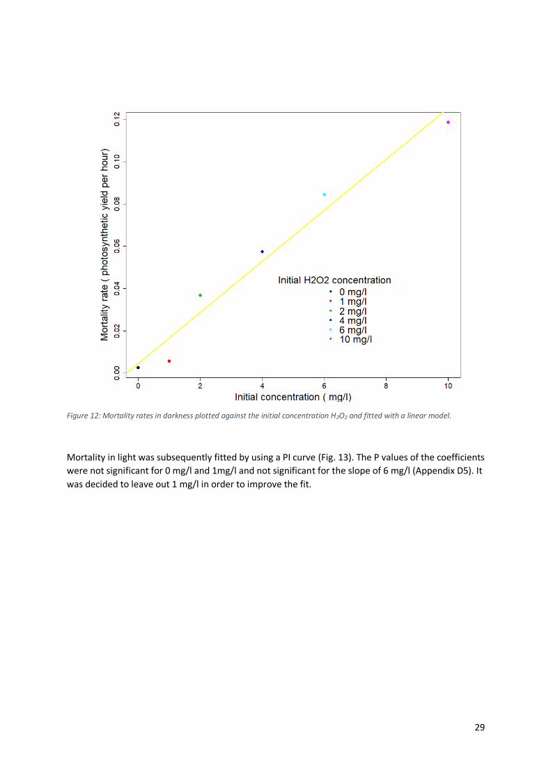
Interestingly, mortality in darkness appeared to increase more linearly with concentration compared
to mortality in light (Fig. 11), which is also observed when plotting mortality rates in darkness against
the initial concentration of H2O2 (Fig.12). The coefficients in this data fit were significant only for the
slope (Appendix D4).
28
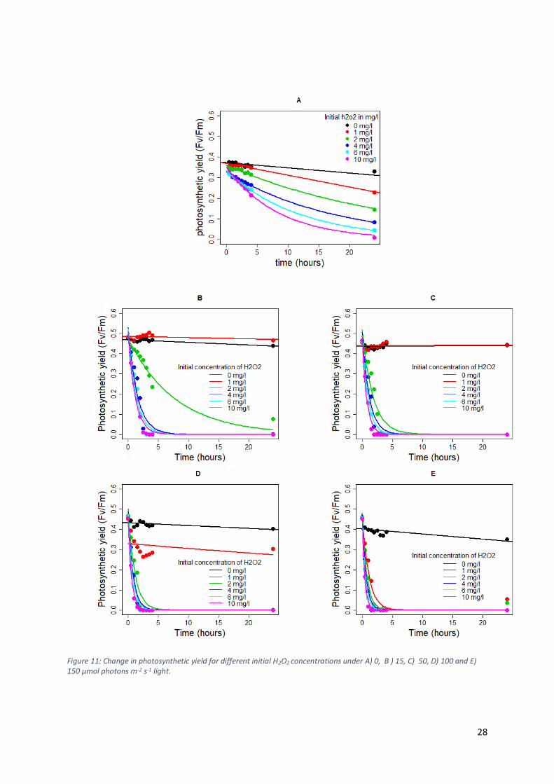
Figure 11: Change in photosynthetic yield for different initial H2O2 concentrations under A) 0, B ) 15, C) 50, D) 100 and E) 150 µmol photons m-2 s-1 light.
29
Figure 12: Mortality rates in darkness plotted against the initial concentration H2O2 and fitted with a linear model.
Mortality in light was subsequently fitted by using a PI curve (Fig. 13). The P values of the coefficients
were not significant for 0 mg/l and 1mg/l and not significant for the slope of 6 mg/l (Appendix D5). It
was decided to leave out 1 mg/l in order to improve the fit.
30
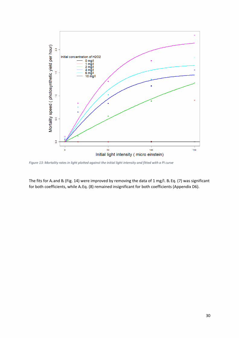
Figure 13: Mortality rates in light plotted against the initial light intensity and fitted with a PI curve
The fits for Al and Bl (Fig. 14) were improved by removing the data of 1 mg/l. Bl Eq. (7) was significant
for both coefficients, while Al Eq. (8) remained insignificant for both coefficients (Appendix D6).
31
Figure 14: Coefficients Al (Eq.7 )and Bl (Eq.8 ) of the mortality M (Eq.6) plotted against initial H2O2 concentrations. For Bl data for 1mg/l was omitted and for Al 1 mg/l and 2mg/l was omitted.
8.2. Phase 2: Lab validation
Degradation of H2O2 appears to be greatest for 1 mg/liter and 2 mg/liter and decreases considerably
with higher concentrations. This effect is also apparent in the fit of the model, which worsens with
increasing concentration of H2O2 (Fig. 15).
32
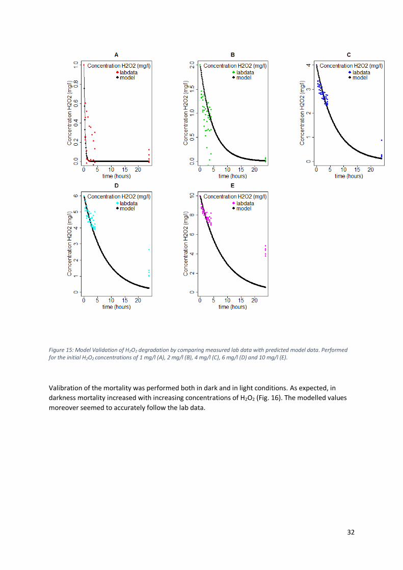
Figure 15: Model Validation of H2O2 degradation by comparing measured lab data with predicted model data. Performed for the initial H2O2 concentrations of 1 mg/l (A), 2 mg/l (B), 4 mg/l (C), 6 mg/l (D) and 10 mg/l (E).
Valibration of the mortality was performed both in dark and in light conditions. As expected, in
darkness mortality increased with increasing concentrations of H2O2 (Fig. 16). The modelled values
moreover seemed to accurately follow the lab data.
33
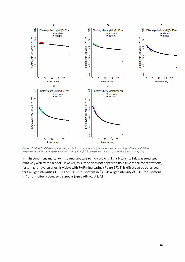
Figure 16: Model validation of mortality in darkness by comparing measured lab data with predicted model data. Performed for the initial H2O2 concentrations of 1 mg/l (A), 2 mg/l (B), 4 mg/l (C), 6 mg/l (D) and 10 mg/l (E).
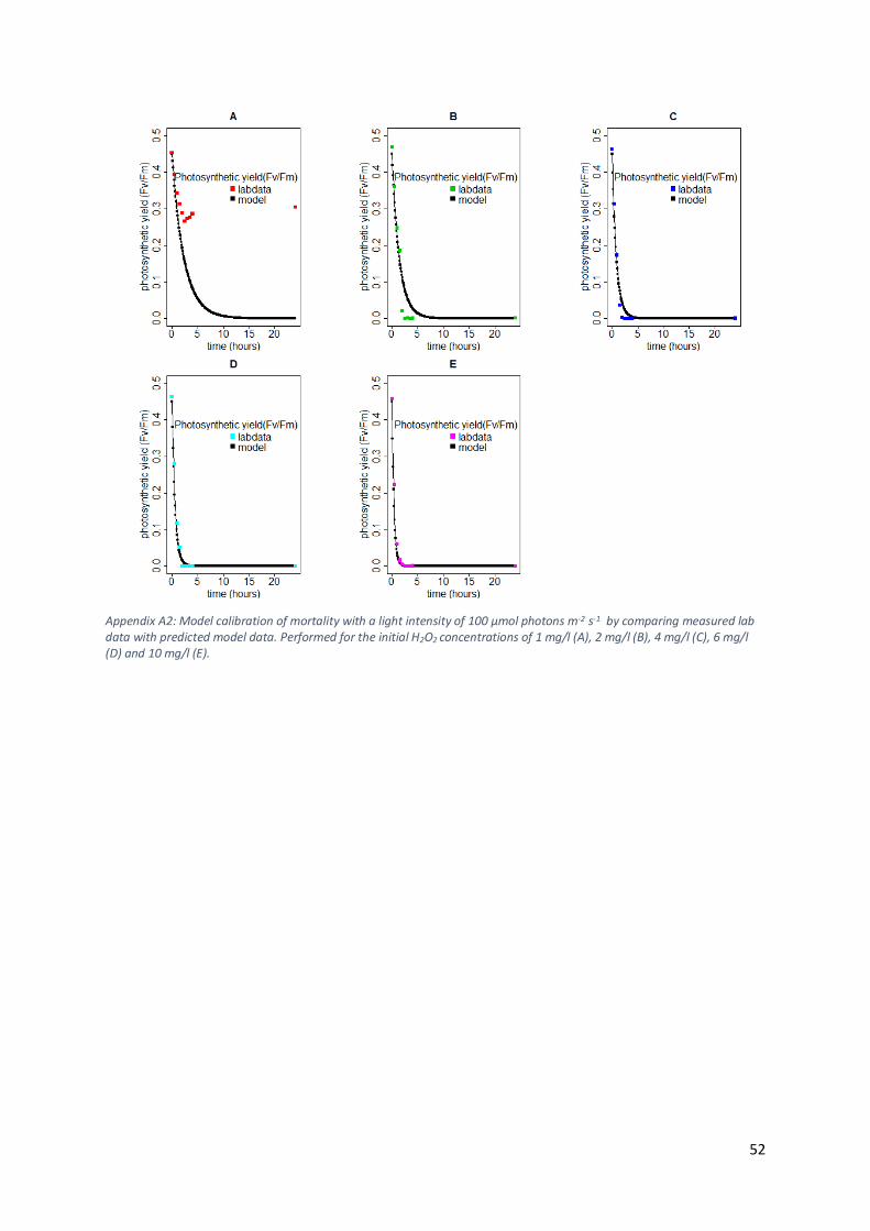
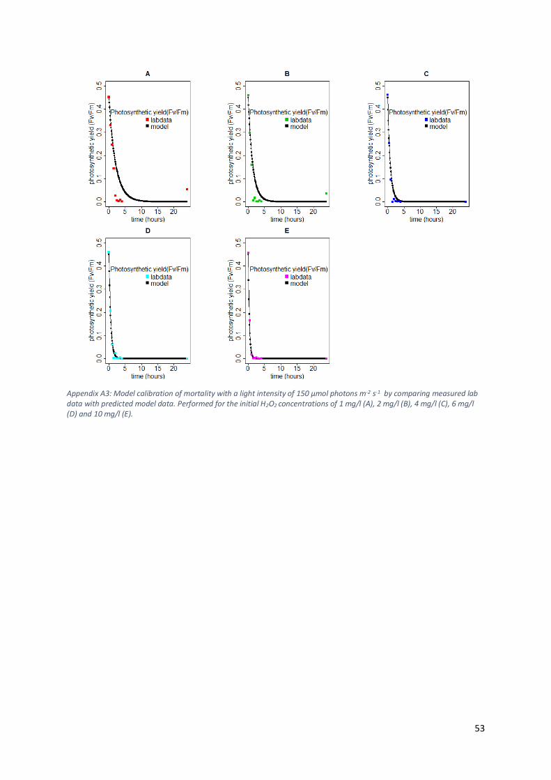
In light conditions mortality in general appears to increase with light intensity. This was predicted
relatively well by the model. However, this trend does not appear to hold true for all concentrations;
for 1 mg/l a reverse effect is visible with Fv/Fm increasing (Figure 17). This effect can be perceived
for the light intensities 15, 50 and 100 µmol photons m-2 s-1. At a light intensity of 150 µmol photons
m-2 s-1 this effect seems to disappear (Appendix A1, A2, A3).
34
Figure 17: Model validation of mortality with a light intensity of 50 µmol photons m-2 s-1 by comparing measured lab data with predicted model data. Performed for the initial H2O2 concentrations of 1 mg/l (A), 2 mg/l (B), 4 mg/l (C), 6 mg/l (D) and 10 mg/l (E).
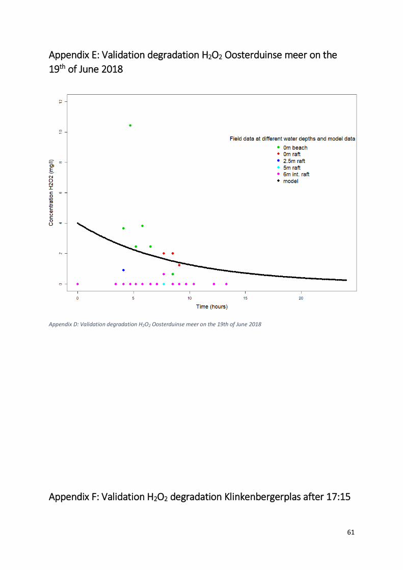
8.3. Phase 3: Field validation
8.3.1. Validation H2O2
The predicted degradation of H2O2 was validated with two treatments datasets: Klinkenbergerplas
on the 15th of June 2017 and Oosterduinse meer on the 8th of August 2018. For the treatment on the
19th of June at the Oosterduinse meer not enough data points for H2O2 were available (Appendix D).
It was therefore decided to refrain from using this dataset in the validations of the degradation of
H2O2 and mortality.
35
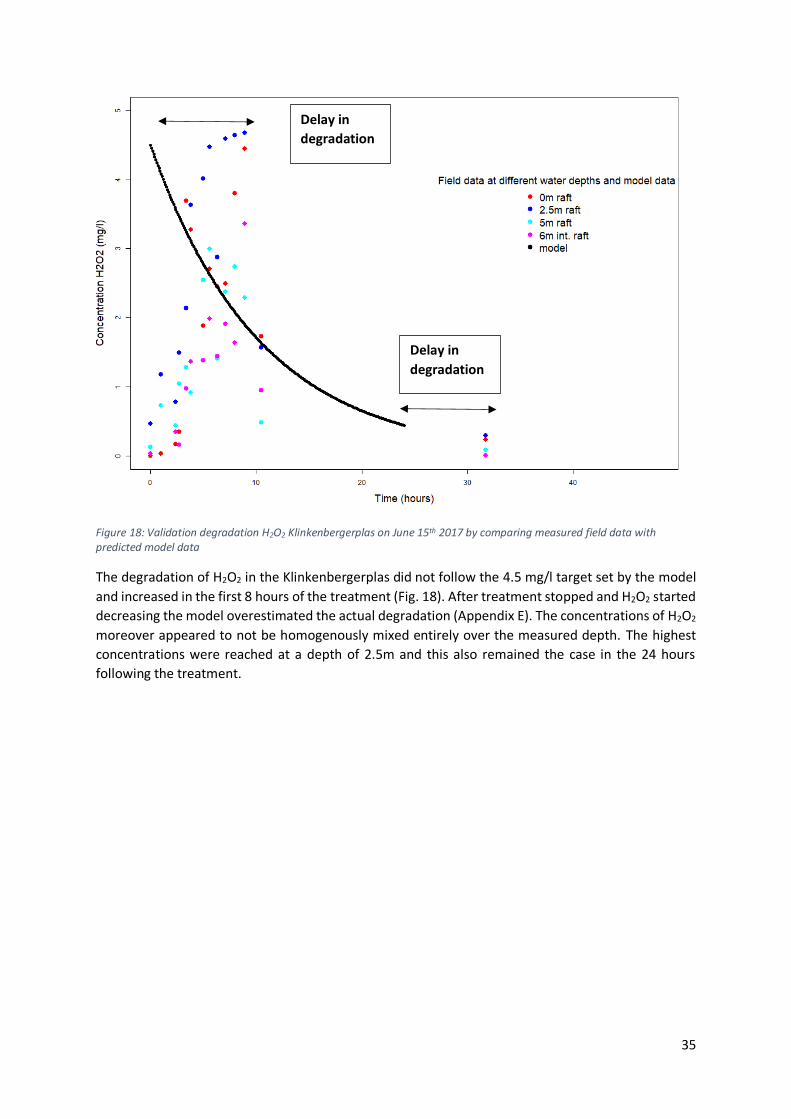
Figure 18: Validation degradation H2O2 Klinkenbergerplas on June 15th 2017 by comparing measured field data with predicted model data
The degradation of H2O2 in the Klinkenbergerplas did not follow the 4.5 mg/l target set by the model
and increased in the first 8 hours of the treatment (Fig. 18). After treatment stopped and H2O2 started
decreasing the model overestimated the actual degradation (Appendix E). The concentrations of H2O2
moreover appeared to not be homogenously mixed entirely over the measured depth. The highest
concentrations were reached at a depth of 2.5m and this also remained the case in the 24 hours
following the treatment.
Delay in
degradation
Delay in
degradation
36
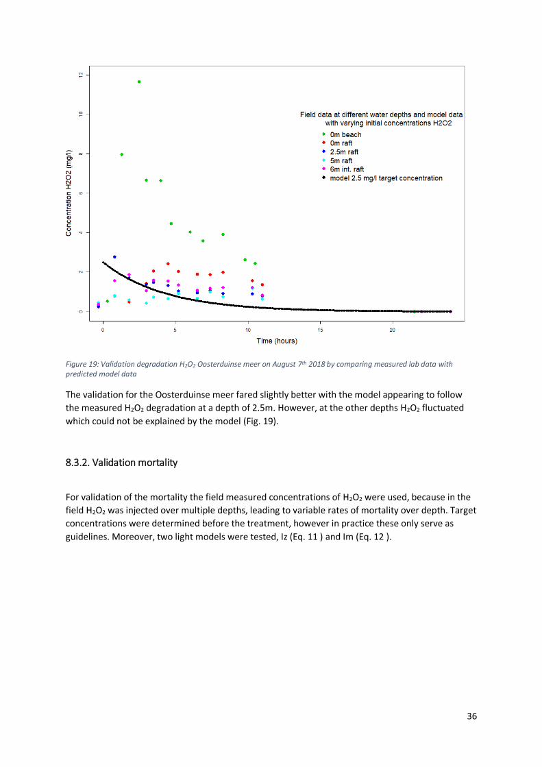
Figure 19: Validation degradation H2O2 Oosterduinse meer on August 7th 2018 by comparing measured lab data with predicted model data
The validation for the Oosterduinse meer fared slightly better with the model appearing to follow
the measured H2O2 degradation at a depth of 2.5m. However, at the other depths H2O2 fluctuated
which could not be explained by the model (Fig. 19).
8.3.2. Validation mortality
For validation of the mortality the field measured concentrations of H2O2 were used, because in the
field H2O2 was injected over multiple depths, leading to variable rates of mortality over depth. Target
concentrations were determined before the treatment, however in practice these only serve as
guidelines. Moreover, two light models were tested, Iz (Eq. 11 ) and Im (Eq. 12 ).
37
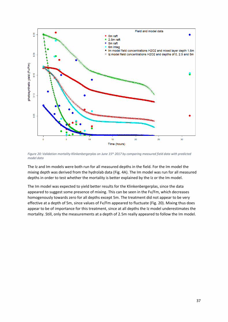
Figure 20: Validation mortality Klinkenbergerplas on June 15th 2017 by comparing measured field data with predicted model data
The Iz and Im models were both run for all measured depths in the field. For the Im model the
mixing depth was derived from the hydrolab data (Fig. 4A). The Im model was run for all measured
depths in order to test whether the mortality is better explained by the Iz or the Im model.
The Im model was expected to yield better results for the Klinkenbergerplas, since the data
appeared to suggest some presence of mixing. This can be seen in the Fv/Fm, which decreases
homogenously towards zero for all depths except 5m. The treatment did not appear to be very
effective at a depth of 5m, since values of Fv/Fm appeared to fluctuate (Fig. 20). Mixing thus does
appear to be of importance for this treatment, since at all depths the Iz model underestimates the
mortality. Still, only the measurements at a depth of 2.5m really appeared to follow the Im model.
38
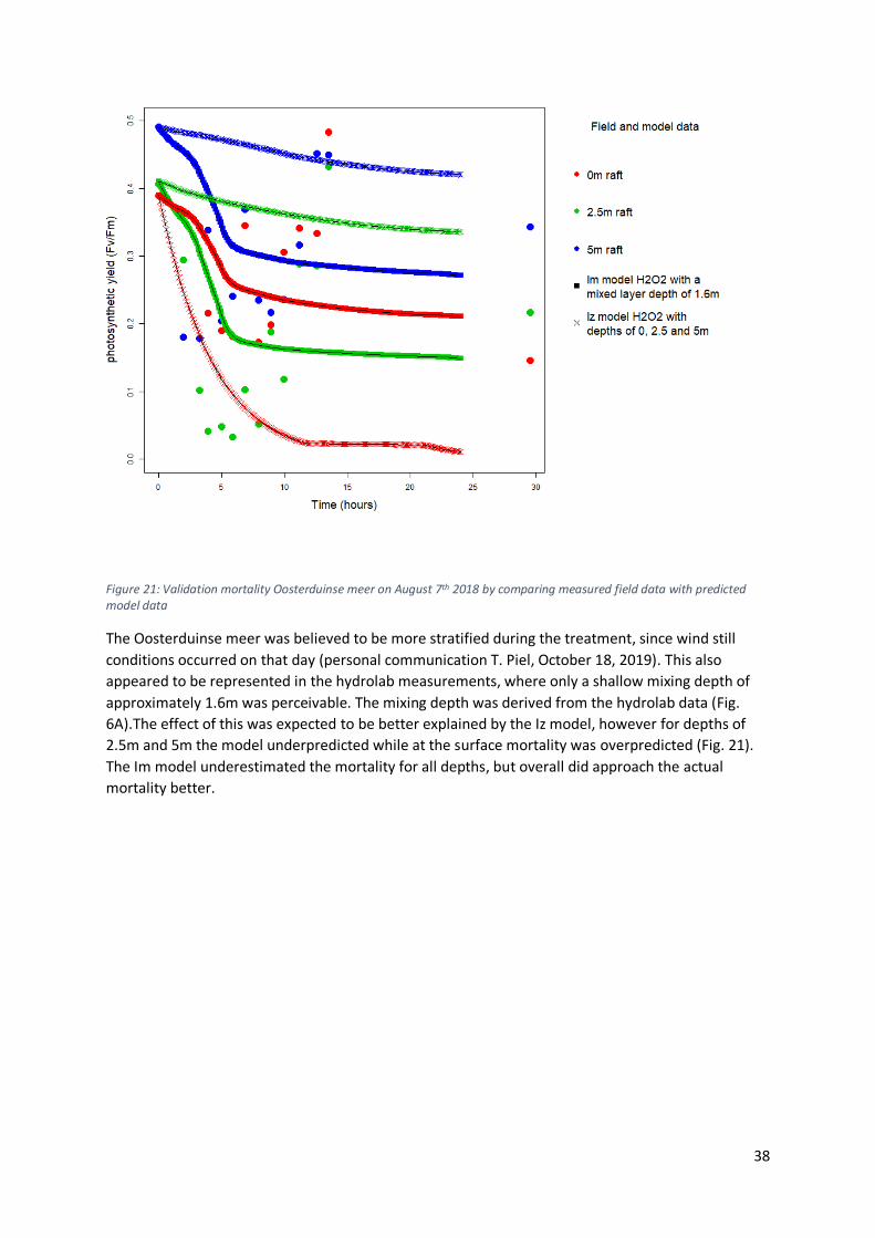
Figure 21: Validation mortality Oosterduinse meer on August 7th 2018 by comparing measured field data with predicted model data
The Oosterduinse meer was believed to be more stratified during the treatment, since wind still
conditions occurred on that day (personal communication T. Piel, October 18, 2019). This also
appeared to be represented in the hydrolab measurements, where only a shallow mixing depth of
approximately 1.6m was perceivable. The mixing depth was derived from the hydrolab data (Fig.
6A).The effect of this was expected to be better explained by the Iz model, however for depths of
2.5m and 5m the model underpredicted while at the surface mortality was overpredicted (Fig. 21).
The Im model underestimated the mortality for all depths, but overall did approach the actual
mortality better.
39
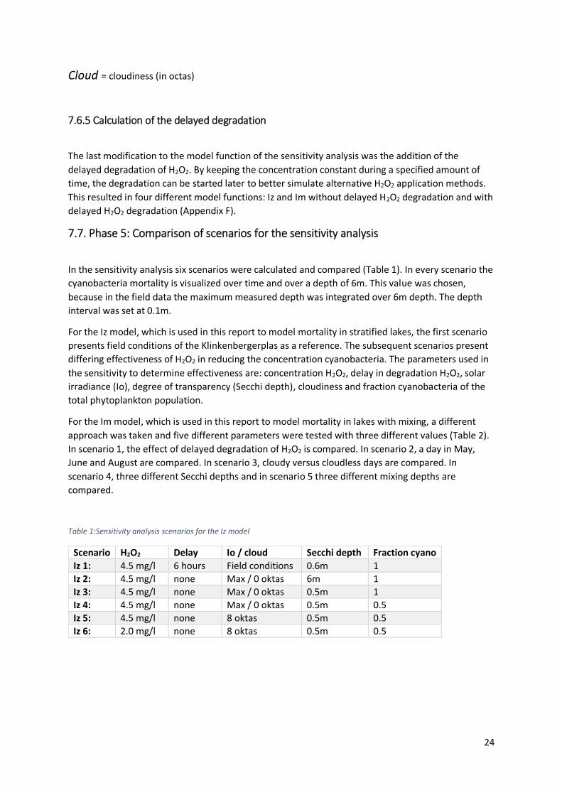
8.4. Phase 5: Sensitivity analysis
8.4.1 Cloud modification factor (CMF)
Figure 22: Cloud modification factor.
The ratios appeared to generally decrease with increasing cloudiness, which was expected (Fig. 22).
Interestingly, the relation appears to be roughly linear from 0 to 6 octas. The greater decrease after
6 octas could be explained by indirect light becoming the dominant source of light, due to increased
cloud coverage. The power model was chosen over the polynomial due to the higher significance of
the slope coefficient (Appendix D7).
8.4.2 Iz model
In the Iz model three parameters appear to be most influential to the effectiveness of H2O2. The
turbidity and the concentration or fraction of cyanobacteria seem to be most important during the
entire treatment, while the effect of delayed degradation of H2O2 becomes visible later in the day.
In reference scenario 1 (Fig. 23), algae are killed down to a depth of around 3m, which is higher than
any scenario except scenario 2 (Fig. 24). This difference in mortality gradually changes over the
course of the treatment, which is explained by the delayed degradation in the reference scenario.
This effect is most apparent 24 hours after the treatment, where in other scenarios mortality
stagnates, because of the lower concentrations H2O2.
40
Figure 23: Scenario 1 Iz model
Figure 24: Scenario 2 Iz model
The impact of turbidity is most perceivable between scenarios 2 and 3 (Fig. 24 & Fig. 25), where in
the former case all algae are deceased over the entire visualized depth, while in the latter case
complete mortality only occurs down to a depth of 2m. Yet, a photosynthetic reduction of roughly
50% is still visible for the rest of the water column.
Figure 25: Scenario 3 Iz model
41
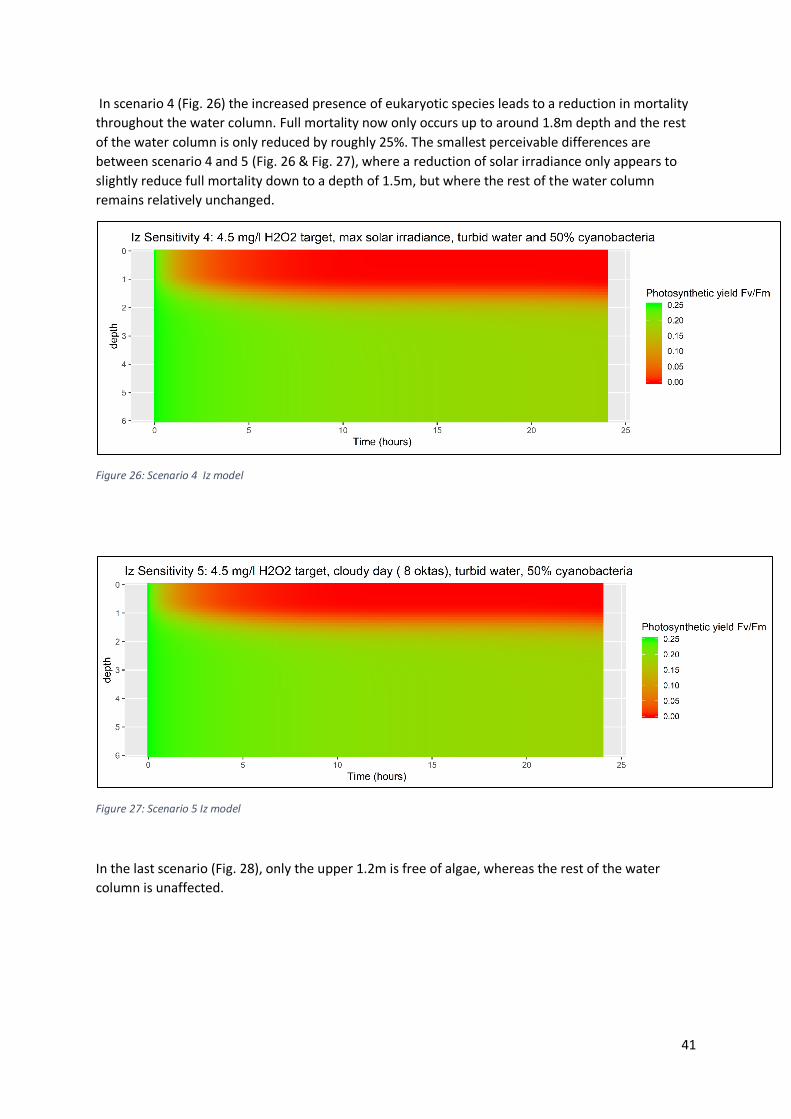
In scenario 4 (Fig. 26) the increased presence of eukaryotic species leads to a reduction in mortality
throughout the water column. Full mortality now only occurs up to around 1.8m depth and the rest
of the water column is only reduced by roughly 25%. The smallest perceivable differences are
between scenario 4 and 5 (Fig. 26 & Fig. 27), where a reduction of solar irradiance only appears to
slightly reduce full mortality down to a depth of 1.5m, but where the rest of the water column
remains relatively unchanged.
Figure 26: Scenario 4 Iz model
Figure 27: Scenario 5 Iz model
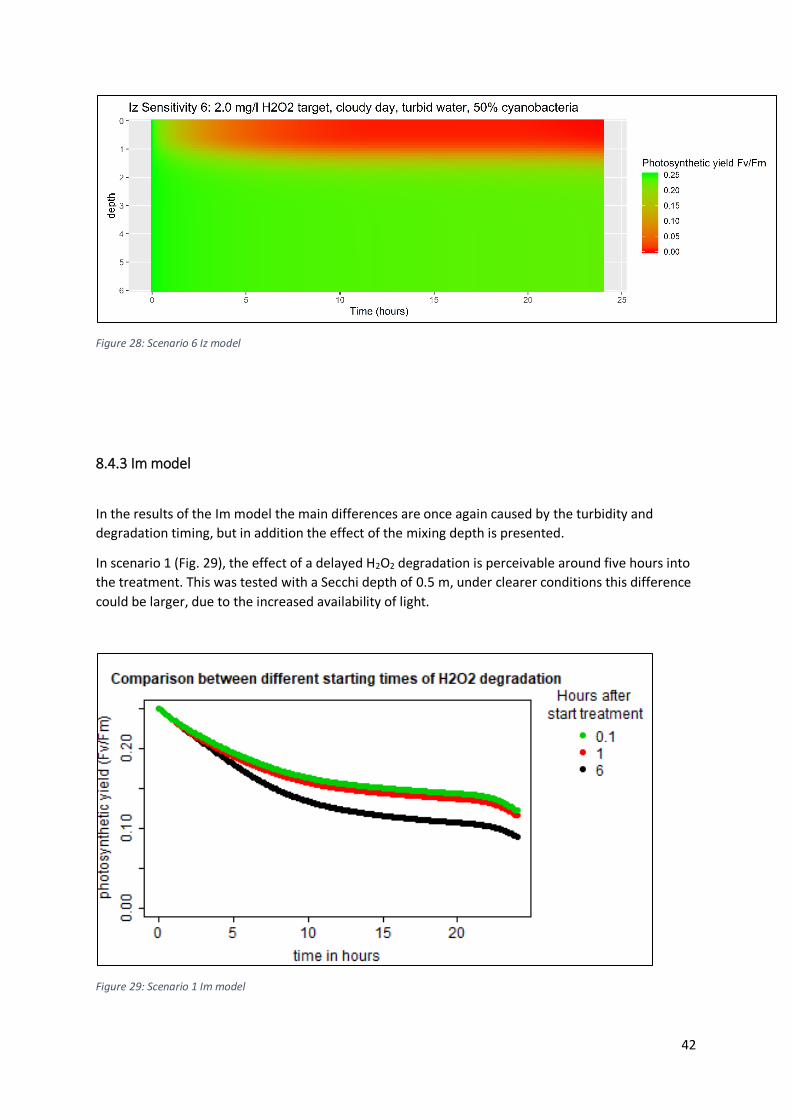
In the last scenario (Fig. 28), only the upper 1.2m is free of algae, whereas the rest of the water
column is unaffected.
42
Figure 28: Scenario 6 Iz model
8.4.3 Im model
In the results of the Im model the main differences are once again caused by the turbidity and
degradation timing, but in addition the effect of the mixing depth is presented.
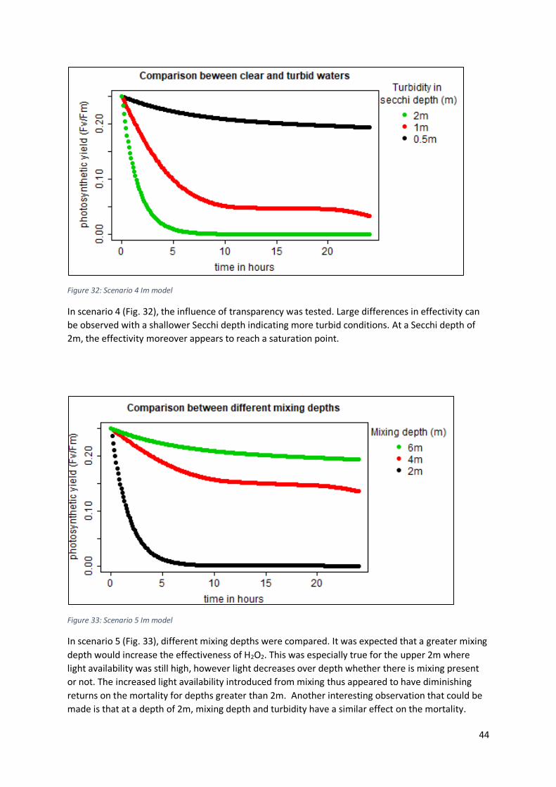
In scenario 1 (Fig. 29), the effect of a delayed H2O2 degradation is perceivable around five hours into
the treatment. This was tested with a Secchi depth of 0.5 m, under clearer conditions this difference
could be larger, due to the increased availability of light.
Figure 29: Scenario 1 Im model
43
Figure 30: Scenario 2 Im model
Figure 31: Scenario 3 Im model
In scenario 2 (Fig. 30) and 3 (Fig. 31), no big differences are perceivable in mortality between days
and between sunny and cloudy days. The relative influence of cloudiness seems to be even smaller
in the Im model than in the Iz model. This suggests that solar irradiance at the surface might not be
the most important factor and is in most cases not an issue.
44
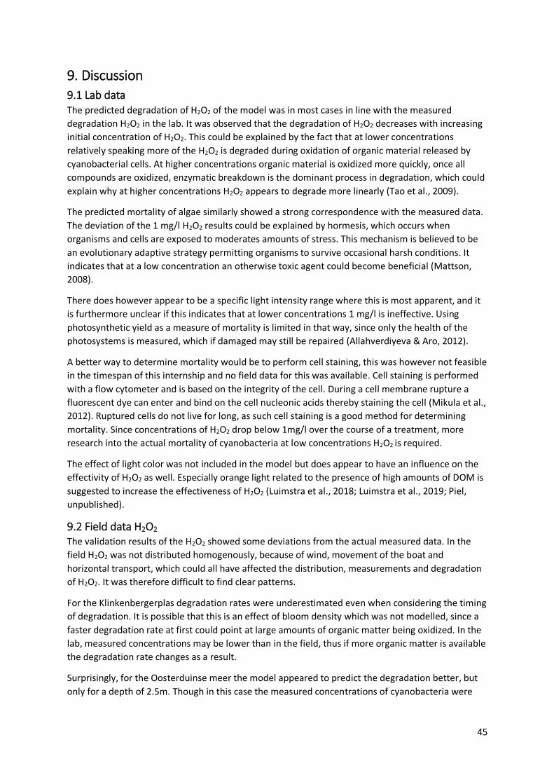
Figure 32: Scenario 4 Im model
In scenario 4 (Fig. 32), the influence of transparency was tested. Large differences in effectivity can
be observed with a shallower Secchi depth indicating more turbid conditions. At a Secchi depth of
2m, the effectivity moreover appears to reach a saturation point.
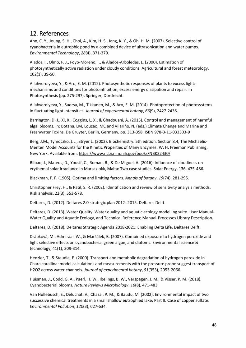
Figure 33: Scenario 5 Im model
In scenario 5 (Fig. 33), different mixing depths were compared. It was expected that a greater mixing
depth would increase the effectiveness of H2O2. This was especially true for the upper 2m where
light availability was still high, however light decreases over depth whether there is mixing present
or not. The increased light availability introduced from mixing thus appeared to have diminishing
returns on the mortality for depths greater than 2m. Another interesting observation that could be
made is that at a depth of 2m, mixing depth and turbidity have a similar effect on the mortality.
45
9. Discussion
9.1 Lab data The predicted degradation of H2O2 of the model was in most cases in line with the measured
degradation H2O2 in the lab. It was observed that the degradation of H2O2 decreases with increasing
initial concentration of H2O2. This could be explained by the fact that at lower concentrations
relatively speaking more of the H2O2 is degraded during oxidation of organic material released by
cyanobacterial cells. At higher concentrations organic material is oxidized more quickly, once all
compounds are oxidized, enzymatic breakdown is the dominant process in degradation, which could
explain why at higher concentrations H2O2 appears to degrade more linearly (Tao et al., 2009).
The predicted mortality of algae similarly showed a strong correspondence with the measured data.
The deviation of the 1 mg/l H2O2 results could be explained by hormesis, which occurs when
organisms and cells are exposed to moderates amounts of stress. This mechanism is believed to be
an evolutionary adaptive strategy permitting organisms to survive occasional harsh conditions. It
indicates that at a low concentration an otherwise toxic agent could become beneficial (Mattson,
2008).
There does however appear to be a specific light intensity range where this is most apparent, and it
is furthermore unclear if this indicates that at lower concentrations 1 mg/l is ineffective. Using
photosynthetic yield as a measure of mortality is limited in that way, since only the health of the
photosystems is measured, which if damaged may still be repaired (Allahverdiyeva & Aro, 2012).
A better way to determine mortality would be to perform cell staining, this was however not feasible
in the timespan of this internship and no field data for this was available. Cell staining is performed
with a flow cytometer and is based on the integrity of the cell. During a cell membrane rupture a
fluorescent dye can enter and bind on the cell nucleonic acids thereby staining the cell (Mikula et al.,
2012). Ruptured cells do not live for long, as such cell staining is a good method for determining
mortality. Since concentrations of H2O2 drop below 1mg/l over the course of a treatment, more
research into the actual mortality of cyanobacteria at low concentrations H2O2 is required.
The effect of light color was not included in the model but does appear to have an influence on the
effectivity of H2O2 as well. Especially orange light related to the presence of high amounts of DOM is
suggested to increase the effectiveness of H2O2 (Luimstra et al., 2018; Luimstra et al., 2019; Piel,
unpublished).
9.2 Field data H2O2
The validation results of the H2O2 showed some deviations from the actual measured data. In the
field H2O2 was not distributed homogenously, because of wind, movement of the boat and
horizontal transport, which could all have affected the distribution, measurements and degradation
of H2O2. It was therefore difficult to find clear patterns.
For the Klinkenbergerplas degradation rates were underestimated even when considering the timing
of degradation. It is possible that this is an effect of bloom density which was not modelled, since a
faster degradation rate at first could point at large amounts of organic matter being oxidized. In the
lab, measured concentrations may be lower than in the field, thus if more organic matter is available
the degradation rate changes as a result.
Surprisingly, for the Oosterduinse meer the model appeared to predict the degradation better, but
only for a depth of 2.5m. Though in this case the measured concentrations of cyanobacteria were
46
lower and eukaryotic phytoplankton were present in almost equal concentrations, which could have
explained the differences in degradation over depth.
It must be noted that degradation of H2O2 is based on lab data of a single species of cyanobacteria.
In the field there are many types of organisms and organic material that could have an impact on the
degradation rate of H2O2.
9.3 Field data mortality cyanobacteria The reason for the inaccurate validations of the mortality in both lakes (Fig. 17 & 18) could have
multiple reasons. In the Klinkenbergerplas especially the mortality rate at the surface deviated,
which could be explained by photoinhibition occurring at the surface, which is not considered in the
model.
Whereas in the Oosterduinse meer mortality was mostly underestimated. The effect of eukaryotic
phytoplankton was however approximated, since lab data for this was limited. Ideally lab
experiments with just eukaryotic phytoplankton or experiments with varying ratios of cyanobacteria
and eukaryotic phytoplankton would have to be conducted to more accurately predict the
effectiveness of H2O2. There is also the daily variability of eukaryotic phytoplankton that may be
considered, which could be an additional underlying process.
9.4 Sensitivity analysis The results of the sensitivity analysis were generally in accordance with what was expected, since
the parameters directly influencing the light intensity under water appeared to have the strongest
effect on the effectivity of H2O2 .The effect of cloudiness was nevertheless not as strong as predicted.
On the one hand, this could be because it only directly influences the light intensity at the water
surface. On the other hand, cloudiness was only calculated based on KNMI data from the year 2017.
A better approximation could be retrieved by using the complete data from 1951 to 2019 and for
different times of day.
In addition, the effect of cloud formation and sun angle was not considered. Cirrus clouds for
instance might even increase the available light intensity as opposed to cloudless conditions
(Kazantzidis et al., 2011). This data was however not readily available and either deemed not
important enough or too complex to include in the model.
Lastly, the assessment of the sensitivity analysis was performed graphically. A statistical or
mathematical method could also be applied to improve the accuracy of the analysis and to better
substantiate the smaller differences (Frey & Patil, 2002).
There are more ways the model could be improved especially regarding the application and spatial
distribution of H2O2 over the treatment lakes. In case of the former, the way delayed degradation of
H2O2 is implemented in the model, is not entirely accurate with how it occurs in the field, where
concentrations steadily increase until the target concentration is reached. In case of the latter, not
much spatial data is available except for measured concentrations H2O2. The model should perhaps
also introduce the capability of algae to recover if photosynthetic is to be used as the primary
indicator for vitality.
47
10. Conclusions
The algicidal capabilities of H2O2 have been thoroughly tested over the last decades, yet thus far no
model had been developed that could predict the effectiveness of H2O2 in combatting cyanobacterial
blooms in the field. This report and associated model attempted to resolve these knowledge gaps.
Ultimately, the degradation of H2O2 and mortality of cyanobacteria appear to be sufficiently
predicted under lab conditions. Specifically, the mortality in light is predicted well for concentrations
of 2mg/l and higher.
In the field however, conditions are more variable and appear to require a substantial amount of
data to approach field scenarios, much of which was not available during the development of this
model. The sensitivity analysis indicates that treating early in bloom development when turbidity is
low and there is more mixing through the water column could be a good strategy, since the lower
amount of solar irradiance earlier in May does not appear to affect the effectiveness of H2O2. Based
on the limited data, eukaryotic phytoplankton also appear to be a factor in determining the
effectivity throughout the treatment and are important to consider during treatments, due to their
ability to degrade H2O2. The effect of the delay in H2O2 degradation conversely only appears to be
apparent on the next day, where under normal application H2O2 would have lost most of its
effectiveness. This could be beneficial, since light is the most important factor and ideally
degradation should only be allowed to start once darkness sets in, though in reality keeping
concentrations constant is rather difficult. Cloudiness moreover does not appear to be a primary
influence, since under these conditions enough light is still available. There could be situations
where the conditions are simply not optimal enough, such as a low fraction of cyanobacteria,
absence of mixing or high turbidity and in those cases alternative methods such as flock and lock
should be applied.
Ultimately, it does not appear to matter when H2O2 is added during daylight, but rather for how long
and under which light specific conditions, such as turbidity and presence of mixing. Even in cloudy
conditions when light intensity is reduced, the effectiveness of H2O2 remains relatively stable.
11. Recommendations While only general recommendations and strategies may be derived from this model, it is
nevertheless a good basis to start with. It is recommended that at least frequent hydrolab
measurements should be taken before during and after treatments, since the turbidity and vertical
distribution of cyanobacteria are essential factors that may impact the effectiveness of H2O2 in the
field. In addition, more pretests should be conducted and analyzed in the lab, so a wider range of
field conditions can be captured, which could thereafter be used to improve the model. The model
should also be expanded: to include more species of phytoplankton, to more accurately predict light
over depth, to model recovery from H2O2 damage and to consider the application and spatial
distribution of H2O2.
48
12. References Ahn, C. Y., Joung, S. H., Choi, A., Kim, H. S., Jang, K. Y., & Oh, H. M. (2007). Selective control of
cyanobacteria in eutrophic pond by a combined device of ultrasonication and water pumps.
Environmental Technology, 28(4), 371-379.
Alados, I., Olmo, F. J., Foyo-Moreno, I., & Alados-Arboledas, L. (2000). Estimation of
photosynthetically active radiation under cloudy conditions. Agricultural and forest meteorology,
102(1), 39-50.
Allahverdiyeva, Y., & Aro, E. M. (2012). Photosynthetic responses of plants to excess light:
mechanisms and conditions for photoinhibition, excess energy dissipation and repair. In
Verspagen, J. M., Passarge, J., Jöhnk, K. D., Visser, P. M., Peperzak, L., Boers, P., ... & Huisman, J.
(2006). Water management strategies against toxic Microcystis blooms in the Dutch delta. Ecological
applications, 16(1), 313-327.
Visser, P., Ibelings, B. A. S., Van Der Veer, B., Koedood, J. A. N., & Mur, R. (1996). Artificial mixing
prevents nuisance blooms of the cyanobacterium Microcystis in Lake Nieuwe Meer, the Netherlands.
Freshwater Biology, 36(2), 435-450.
Waajen, G., van Oosterhout, F., Douglas, G., & Lürling, M. (2016). Management of eutrophication in
Lake De Kuil (The Netherlands) using combined flocculant–Lanthanum modified bentonite
treatment. Water research, 97, 83-95.
Weenink, E. F., Luimstra, V. M., Schuurmans, J. M., Van Herk, M. J., Visser, P. M., & Matthijs, H. C.
(2015). Combatting cyanobacteria with hydrogen peroxide: a laboratory study on the consequences
for phytoplankton community and diversity. Frontiers in microbiology, 6, 714.
51
Appendix A: Calibration lab results
Appendix A1: Model calibration of mortality with a light intensity of 15 µmol photons m-2 s-1 by comparing measured lab data with predicted model data. Performed for the initial H2O2 concentrations of 1 mg/l (A), 2 mg/l (B), 4 mg/l (C), 6 mg/l (D) and 10 mg/l (E).
52
Appendix A2: Model calibration of mortality with a light intensity of 100 µmol photons m-2 s-1 by comparing measured lab data with predicted model data. Performed for the initial H2O2 concentrations of 1 mg/l (A), 2 mg/l (B), 4 mg/l (C), 6 mg/l (D) and 10 mg/l (E).
53
Appendix A3: Model calibration of mortality with a light intensity of 150 µmol photons m-2 s-1 by comparing measured lab data with predicted model data. Performed for the initial H2O2 concentrations of 1 mg/l (A), 2 mg/l (B), 4 mg/l (C), 6 mg/l (D) and 10 mg/l (E).
54
Appendix B: hydrolab data Klinkenbergerplas
Appendix B1: Hydrolab PAR measurements Klinkenbergerplas on the 15th of June 2017 at 07:38 over A) the first four meters and B) over the total measured depth.
A
B
55
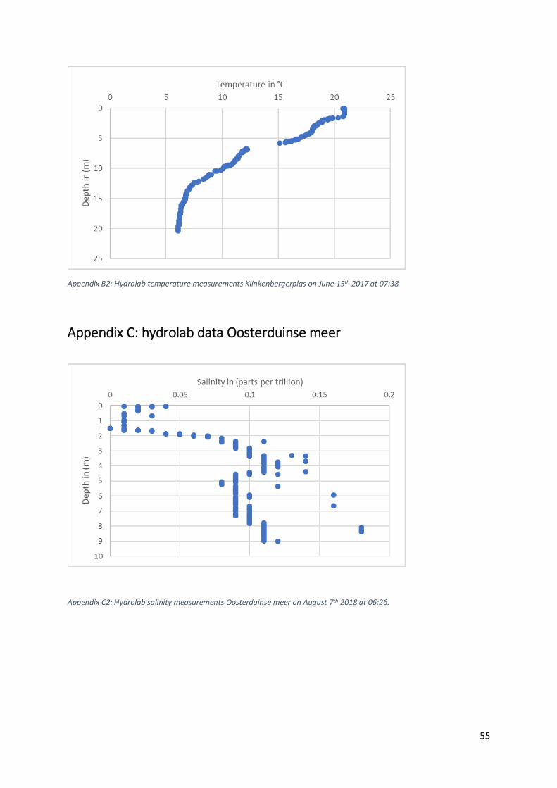
Appendix B2: Hydrolab temperature measurements Klinkenbergerplas on June 15th 2017 at 07:38
Appendix C: hydrolab data Oosterduinse meer
Appendix C2: Hydrolab salinity measurements Oosterduinse meer on August 7th 2018 at 06:26.
56
Appendix C1: Hydrolab PAR measurements Oosterduinse meer on August 7th 2018 at 09:30 over A) the first two meters and B) over the entire measured depth.
A
B
57
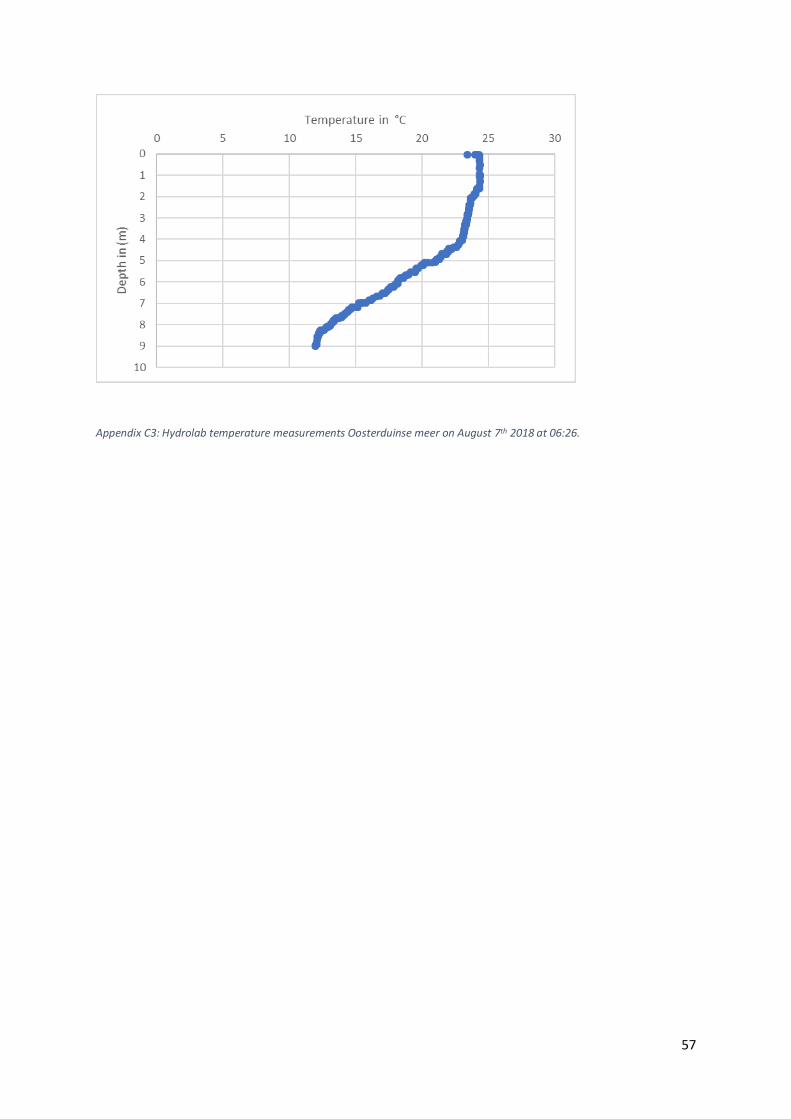
Appendix C3: Hydrolab temperature measurements Oosterduinse meer on August 7th 2018 at 06:26.
58
Appendix D: Statistical data of data fits
Appendix D1: P values data fit of lab measured H2O2 (Eq. 1). Coefficient A is the intercept a and coefficient B is the slope b
Appendix D2: P values of data fit degradation rate H2O2 plotted against the initial concentration H2O2 (Eq. 2). Coefficient A is Vmax and coefficient B is K.
P values 1 mg/l 0 micro einstein
1 mg/l 15 micro einstein
1 mg/l 50 micro einstein
1 mg/l 100 micro einstein
1 mg/l 150 micro einstein
A coefficient 6.731524e-07 ***
1.879864e-07 ***
2.518551e-05 ***
7.001895e-05 ***
0.0006295768 ***
B coefficient 7.699017e-05 ***
2.816012e-04 ***
2.621269e-02 *
3.190513e-02 *
0.0465879389 *
2 mg/l 0 micro einstein
2 mg/l 15 micro einstein
2 mg/l 50 micro einstein
2 mg/l 100 micro einstein
2 mg/l 150 micro einstein
A coefficient 2.081202e-07 ***
8.211407e-08 ***
2.023949e-06 ***
3.362717e-06 ***
5.875849e-08 ***
B coefficient 2.983239e-04 ***
5.545858e-06 ***
2.454306e-04 ***
3.106421e-03 **
7.578208e-04 ***
4 mg/l 0 micro einstein
4 mg/l 15 micro einstein
4 mg/l 50 micro einstein
4 mg/l 100 micro einstein
4 mg/l 150 micro einstein
A coefficient 7.761422e-09 ***
4.288614e-09 ***
8.997480e-09 ***
4.730836e-10 ***
2.903208e-09 ***
B coefficient 2.423381e-04 ***
2.555018e-04 ***
2.403977e-04 ***
3.723957e-05 ***
5.865279e-04 ***
6 mg/l 0 micro einstein
6 mg/l 15 micro einstein
6 mg/l 50 micro einstein
6 mg/l 100 micro einstein
6 mg/l 150 micro einstein
A coefficient 2.449103e-09 ***
4.377453e-11 ***
1.332911e-09 ***
1.867051e-10 ***
3.122503e-10 ***
B coefficient 5.232671e-04 ***
1.848886e-05 ***
3.013800e-04 ***
4.123213e-05 ***
6.351069e-04 ***
10 mg/l 0 micro einstein
10 mg/l 15 micro einstein
10 mg/l 50 micro einstein
10 mg/l 100 micro einstein
10 mg/l 150 micro einstein
A coefficient 2.957502e-10 ***
2.109152e-11 ***
6.731219e-10 ***
5.349858e-10 ***
3.343516e-10 ***
B coefficient 7.438460e-04 ***
3.578844e-05 ***
1.073004e-03 **
6.003899e-04 ***
1.070948e-03 **
P value A coefficient B coefficient
2.116837e-01 8.173057e-19 ***
59
Appendix D3: P values data fit of lab measured Fv/Fm (Eq. 4). Coefficient A is the intercept a and coefficient B is the slope b.
P values 0 mg/l 0 micro einstein
0 mg/l 15 micro einstein
0 mg/l 50 micro einstein
0 mg/l 100 micro einstein
0 mg/l 150 micro einstein
A coefficient 6.99E-12 ***
1.99E-16 ***
4.38E-13 ***
1.13E-12 ***
8.27E-11 ***
B coefficient 1.78E-03 **
1.25E-03 **
7.76E-01 8.73E-02 5.99E-02
1 mg/l 0 micro einstein
1 mg/l 15 micro einstein
1 mg/l 50 micro einstein
1 mg/l 100 micro einstein
1 mg/l 150 micro einstein
A coefficient 3.93E-13 ***
6.91E-14 ***
3.05E-13 ***
6.89E-07 ***
1.30E-06 ***
B coefficient 5.76E-07 ***
3.50E-01 7.74E-01 4.82E-01 8.54E-05 ***
2 mg/l 0 micro einstein
2 mg/l 15 micro einstein
2 mg/l 50 micro einstein
2 mg/l 100 micro einstein
2 mg/l 150 micro einstein
A coefficient 3.32E-12 ***
8.43E-09 ***
1.37E-05 ***
1.79E-06 ***
4.82E-07 ***
B coefficient 9.53E-07 ***
2.01E-04 ***
6.64E-04 ***
1.12E-04 ***
5.83E-05 ***
4 mg/l 0 micro einstein
4 mg/l 15 micro einstein
4 mg/l 50 micro einstein
4 mg/l 100 micro einstein
4 mg/l 150 micro einstein
A coefficient 4.93E-13 ***
7.28E-06 ***
2.68E-06 ***
2.11E-07 ***
1.69E-08 ***
B coefficient 4.55E-08 ***
3.53E-04 ***
1.54E-04 ***
2.41E-05 ***
3.79E-06 ***
6 mg/l 0 micro einstein
6 mg/l 15 micro einstein
6 mg/l 50 micro einstein
6 mg/l 100 micro einstein
6 mg/l 150 micro einstein
A coefficient 1.91E-13 ***
1.49E-06 ***
6.26E-07 ***
7.33E-09 ***
6.52E-10 ***
B coefficient 6.18E-09 ***
8.49E-05 ***
5.08E-05 ***
1.22E-06 ***
2.51E-07 ***
10 mg/l 0 micro einstein
10 mg/l 15 micro einstein
10 mg/l 50 micro einstein
10 mg/l 100 micro einstein
10 mg/l 150 micro einstein
A coefficient 6.49E-11 ***
1.05E-07 ***
6.57E-08 ***
1.05E-09 ***
4.74E-10 ***
B coefficient 4.94E-07 ***
7.49E-06 ***
9.33E-06 ***
3.54E-07 ***
4.15E-07 ***
60
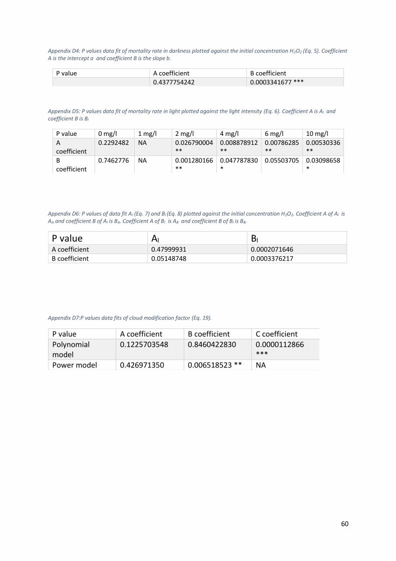
Appendix D4: P values data fit of mortality rate in darkness plotted against the initial concentration H2O2 (Eq. 5). Coefficient A is the intercept a and coefficient B is the slope b.
Appendix D5: P values data fit of mortality rate in light plotted against the light intensity (Eq. 6). Coefficient A is Al and coefficient B is Bl
Appendix D6: P values of data fit Al (Eq. 7) and Bl (Eq. 8) plotted against the initial concentration H2O2. Coefficient A of Al is AA and coefficient B of Al is BA. Coefficient A of Bl is AB and coefficient B of Bl is BB.
Appendix D7:P values data fits of cloud modification factor (Eq. 19).
P value A coefficient B coefficient
0.4377754242 0.0003341677 ***
P value 0 mg/l 1 mg/l 2 mg/l 4 mg/l 6 mg/l 10 mg/l
A coefficient
0.2292482 NA 0.026790004 **
0.008878912 **
0.00786285 **
0.00530336 **
B coefficient
0.7462776 NA 0.001280166 **
0.047787830 *
0.05503705
0.03098658 *
P value Al Bl A coefficient 0.47999931 0.0002071646
B coefficient 0.05148748 0.0003376217
P value A coefficient B coefficient C coefficient
Polynomial model
0.1225703548 0.8460422830 0.0000112866 ***
Power model 0.426971350 0.006518523 ** NA
61
Appendix E: Validation degradation H2O2 Oosterduinse meer on the
19th of June 2018
Appendix D: Validation degradation H2O2 Oosterduinse meer on the 19th of June 2018
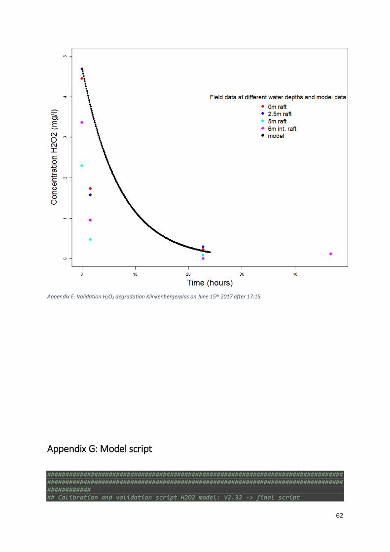
Appendix F: Validation H2O2 degradation Klinkenbergerplas after 17:15
62
Appendix E: Validation H2O2 degradation Klinkenbergerplas on June 15th 2017 after 17:15
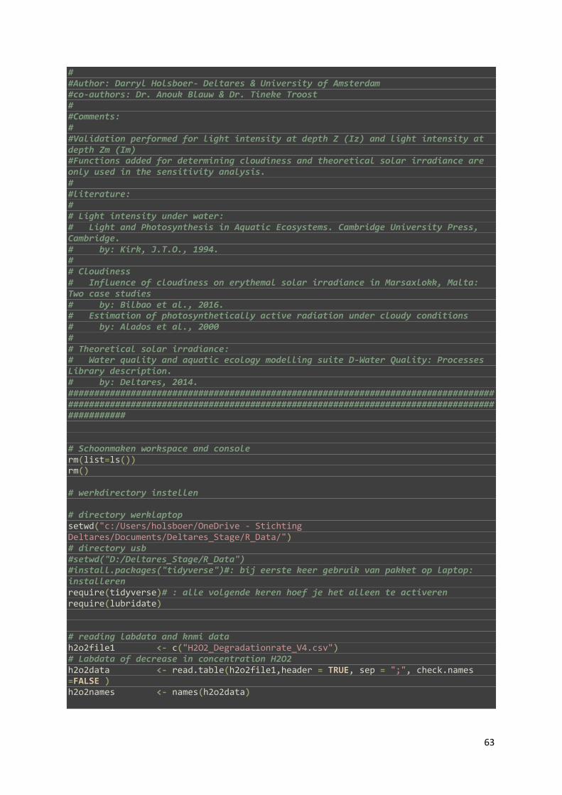
Appendix G: Model script
################################################################################################################################################################################ ## Calibration and validation script H2O2 model: V2.32 -> final script
63
# #Author: Darryl Holsboer- Deltares & University of Amsterdam #co-authors: Dr. Anouk Blauw & Dr. Tineke Troost # #Comments: # #Validation performed for light intensity at depth Z (Iz) and light intensity at depth Zm (Im) #Functions added for determining cloudiness and theoretical solar irradiance are only used in the sensitivity analysis. # #literature: # # Light intensity under water: # Light and Photosynthesis in Aquatic Ecosystems. Cambridge University Press, Cambridge. # by: Kirk, J.T.O., 1994. # # Cloudiness # Influence of cloudiness on erythemal solar irradiance in Marsaxlokk, Malta: Two case studies # by: Bilbao et al., 2016. # Estimation of photosynthetically active radiation under cloudy conditions # by: Alados et al., 2000 # # Theoretical solar irradiance: # Water quality and aquatic ecology modelling suite D-Water Quality: Processes Library description. # by: Deltares, 2014. ############################################################################################################################################################################### # Schoonmaken workspace and console rm(list=ls()) rm() # werkdirectory instellen # directory werklaptop setwd("c:/Users/holsboer/OneDrive - Stichting Deltares/Documents/Deltares_Stage/R_Data/") # directory usb #setwd("D:/Deltares_Stage/R_Data") #install.packages("tidyverse")#: bij eerste keer gebruik van pakket op laptop: installeren require(tidyverse)# : alle volgende keren hoef je het alleen te activeren require(lubridate) # reading labdata and knmi data h2o2file1 <- c("H2O2_Degradationrate_V4.csv") # Labdata of decrease in concentration H2O2 h2o2data <- read.table(h2o2file1,header = TRUE, sep = ";", check.names =FALSE ) h2o2names <- names(h2o2data)
64
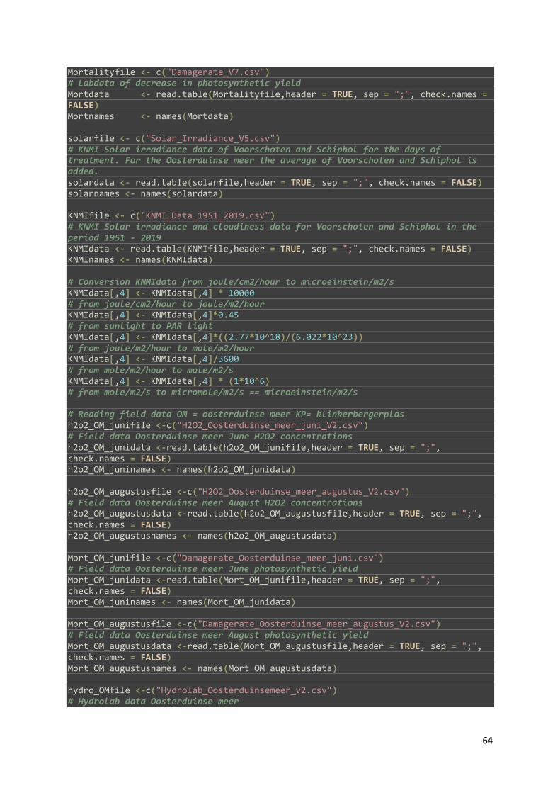
Mortalityfile <- c("Damagerate_V7.csv") # Labdata of decrease in photosynthetic yield Mortdata <- read.table(Mortalityfile,header = TRUE, sep = ";", check.names = FALSE) Mortnames <- names(Mortdata) solarfile <- c("Solar_Irradiance_V5.csv") # KNMI Solar irradiance data of Voorschoten and Schiphol for the days of treatment. For the Oosterduinse meer the average of Voorschoten and Schiphol is added. solardata <- read.table(solarfile,header = TRUE, sep = ";", check.names = FALSE) solarnames <- names(solardata) KNMIfile <- c("KNMI_Data_1951_2019.csv") # KNMI Solar irradiance and cloudiness data for Voorschoten and Schiphol in the period 1951 - 2019 KNMIdata <- read.table(KNMIfile,header = TRUE, sep = ";", check.names = FALSE) KNMInames <- names(KNMIdata) # Conversion KNMIdata from joule/cm2/hour to microeinstein/m2/s KNMIdata[,4] <- KNMIdata[,4] * 10000 # from joule/cm2/hour to joule/m2/hour KNMIdata[,4] <- KNMIdata[,4]*0.45 # from sunlight to PAR light KNMIdata[,4] <- KNMIdata[,4]*((2.77*10^18)/(6.022*10^23)) # from joule/m2/hour to mole/m2/hour KNMIdata[,4] <- KNMIdata[,4]/3600 # from mole/m2/hour to mole/m2/s KNMIdata[,4] <- KNMIdata[,4] * (1*10^6) # from mole/m2/s to micromole/m2/s == microeinstein/m2/s # Reading field data OM = oosterduinse meer KP= klinkerbergerplas h2o2_OM_junifile <-c("H2O2_Oosterduinse_meer_juni_V2.csv") # Field data Oosterduinse meer June H2O2 concentrations h2o2_OM_junidata <-read.table(h2o2_OM_junifile,header = TRUE, sep = ";", check.names = FALSE) h2o2_OM_juninames <- names(h2o2_OM_junidata) h2o2_OM_augustusfile <-c("H2O2_Oosterduinse_meer_augustus_V2.csv") # Field data Oosterduinse meer August H2O2 concentrations h2o2_OM_augustusdata <-read.table(h2o2_OM_augustusfile,header = TRUE, sep = ";", check.names = FALSE) h2o2_OM_augustusnames <- names(h2o2_OM_augustusdata) Mort_OM_junifile <-c("Damagerate_Oosterduinse_meer_juni.csv") # Field data Oosterduinse meer June photosynthetic yield Mort_OM_junidata <-read.table(Mort_OM_junifile,header = TRUE, sep = ";", check.names = FALSE) Mort_OM_juninames <- names(Mort_OM_junidata) Mort_OM_augustusfile <-c("Damagerate_Oosterduinse_meer_augustus_V2.csv") # Field data Oosterduinse meer August photosynthetic yield Mort_OM_augustusdata <-read.table(Mort_OM_augustusfile,header = TRUE, sep = ";", check.names = FALSE) Mort_OM_augustusnames <- names(Mort_OM_augustusdata) hydro_OMfile <-c("Hydrolab_Oosterduinsemeer_v2.csv") # Hydrolab data Oosterduinse meer
65
hydro_OMdata <-read.table(hydro_OMfile,header = TRUE, sep = ";", check.names = FALSE) hydro_OMnames <- names(hydro_OMdata) h2o2_KP_junifile <-c("H2O2_Klinkenberger_plas_juni_V3.csv") # Field data Klinkenberger plas H2O2 concentrations h2o2_KP_junidata <-read.table(h2o2_KP_junifile,header = TRUE, sep = ";", check.names = FALSE) h2o2_KP_juninames <- names(h2o2_KP_junidata) h2o2_KP_juniselectiefile <-c("H2O2_Klinkenberger_plas_juni_selectie_V2.csv") # Field data Klinkenberger plas H2O2 concentrations after 18:00 h2o2_KP_juniselectiedata <-read.table(h2o2_KP_juniselectiefile,header = TRUE, sep = ";", check.names = FALSE) h2o2_KP_juniselectienames <- names(h2o2_KP_juniselectiedata) hydro_KPfile <-c("Hydrolab_Klinkenbergerplas_v2.csv") # Hydrolab data Klinkenberger plas hydro_KPdata <-read.table(hydro_KPfile,header = TRUE, sep = ";", check.names = FALSE) hydro_KPnames <- names(hydro_KPdata) Mort_KPfile <-c("Damagerate_Klinkenberger_plas.csv") # Field data photosynthetic yield Klinkenberger plas Mort_KPdata <-read.table(Mort_KPfile,header = TRUE, sep = ";", check.names = FALSE) Mort_KPnames <-names(Mort_KPdata) # Divide data by 1000. For the KP only the last 3 numbers after the . were written down. Mort_KPdata[,3:6] <- Mort_KPdata[,3:6]/1000 ### Variables ### I_o_time <- solardata[1:261,1] # time in hour I_o_KP <- solardata[1:261,6] # solar irradiance in microeinstein/m2/s. interp_I_o_KP <- approx(I_o_time,I_o_KP,I_o_time) plot(interp_I_o_KP$x,interp_I_o_KP$y) I_o_KP_fun <- approxfun(I_o_time,I_o_KP) I_o_OM_Juni <-solardata[262:522,8] # solar irradiance in microeinstein/m2/s. interp_I_o_OM_Juni <- approx(I_o_time,I_o_OM_Juni,I_o_time) plot(interp_I_o_OM_Juni$x,interp_I_o_OM_Juni$y) I_o_OM_Juni_fun <- approxfun(I_o_time,I_o_OM_Juni) I_o_OM_Aug <- solardata[523:783,8] # solar irradiance in microeinstein/m2/s. interp_I_o_OM_Aug <- approx(I_o_time,I_o_OM_Aug,I_o_time) plot(interp_I_o_OM_Aug$x,interp_I_o_OM_Aug$y) I_o_OM_Aug_fun <-approxfun(I_o_time,I_o_OM_Aug) ### Interpolating field concentrations H2O2 over time ############ H2O2_KP_time <- h2o2_KP_junidata$`Timestep` H2O2_KP_Y1 <- h2o2_KP_junidata$`0m raft` # Field concentrations H2O2 at depth = 0m
66
H2O2_KP_Y2 <- h2o2_KP_junidata$`2.5m raft` # Field concentrations H2O2 at depth = 2.5m H2O2_KP_Y3 <- h2o2_KP_junidata$`5m raft` # Field concentrations H2O2 at depth = 5m H2O2_KP_Y4 <- h2o2_KP_junidata$`6m int. raft` # Field concentrations H2O2 at depth = 6m integrated Interp_KP1 <- approx(H2O2_KP_time,H2O2_KP_Y1,H2O2_KP_time) Interp_KP2 <- approx(H2O2_KP_time,H2O2_KP_Y2,H2O2_KP_time) Interp_KP3 <- approx(H2O2_KP_time,H2O2_KP_Y3,H2O2_KP_time) Interp_KP4 <- approx(H2O2_KP_time,H2O2_KP_Y4,H2O2_KP_time) plot(H2O2_KP_time, h2o2_KP_junidata$`0m raft`, cex=2) points(H2O2_KP_time,Interp_KP1$y, col=2) H2O2_OM_June_time <- h2o2_OM_junidata$`Timestep` H2O2_OM_June_Y1 <- h2o2_OM_junidata$`0m beach` # Field concentrations H2O2 at depth = 0m at the beach H2O2_OM_June_Y2 <- h2o2_OM_junidata$`0m raft` # Field concentrations H2O2 at depth = 0m on the raft H2O2_OM_June_Y3 <- h2o2_OM_junidata$`2.5m raft` # Field concentrations H2O2 at depth = 0m on the raft H2O2_OM_June_Y4 <- h2o2_OM_junidata$`5m raft` # Field concentrations H2O2 at depth = 0m on the raft H2O2_OM_June_Y5 <- h2o2_OM_junidata$`6m int. raft` # Field concentrations H2O2 at depth = 0m on the raft Interp_OM_June1 <- approx(H2O2_OM_June_time,H2O2_OM_June_Y1,H2O2_OM_June_time) Interp_OM_June2 <- approx(H2O2_OM_June_time,H2O2_OM_June_Y2,H2O2_OM_June_time) Interp_OM_June3 <- approx(H2O2_OM_June_time,H2O2_OM_June_Y3,H2O2_OM_June_time) Interp_OM_June4 <- approx(H2O2_OM_June_time,H2O2_OM_June_Y4,H2O2_OM_June_time) Interp_OM_June5 <- approx(H2O2_OM_June_time,H2O2_OM_June_Y5,H2O2_OM_June_time) plot(H2O2_OM_June_time,Interp_OM_June5$y) H2O2_OM_Aug_time <- h2o2_OM_augustusdata$`Timestep` H2O2_OM_Aug_Y1 <- h2o2_OM_augustusdata$`0m beach` # Field concentrations H2O2 at depth = 0m at the beach H2O2_OM_Aug_Y2 <- h2o2_OM_augustusdata$`0m raft` # Field concentrations H2O2 at depth = 0m on the raft H2O2_OM_Aug_Y3 <- h2o2_OM_augustusdata$`2.5m raft` # Field concentrations H2O2 at depth = 0m on the raft H2O2_OM_Aug_Y4 <- h2o2_OM_augustusdata$`5m raft` # Field concentrations H2O2 at depth = 0m on the raft H2O2_OM_Aug_Y5 <- h2o2_OM_augustusdata$`6m int. raft` # Field concentrations H2O2 at depth = 0m on the raft Interp_OM_Aug1 <- approx(H2O2_OM_Aug_time,H2O2_OM_Aug_Y1,H2O2_OM_Aug_time) Interp_OM_Aug2 <- approx(H2O2_OM_Aug_time,H2O2_OM_Aug_Y2,H2O2_OM_Aug_time) Interp_OM_Aug3 <- approx(H2O2_OM_Aug_time,H2O2_OM_Aug_Y3,H2O2_OM_Aug_time) Interp_OM_Aug4 <- approx(H2O2_OM_Aug_time,H2O2_OM_Aug_Y4,H2O2_OM_Aug_time) Interp_OM_Aug5 <- approx(H2O2_OM_Aug_time,H2O2_OM_Aug_Y5,H2O2_OM_Aug_time) plot(H2O2_OM_Aug_time,Interp_OM_Aug3$y) # Gemiddelden berekenen # Input unique() in this case Mortnames can be retrieved by using names()/colnames() on your dataset. meanmort <- sapply(unique(Mortnames), function(g) rowMeans(Mortdata[,Mortnames==g,drop=FALSE])) meanMortdata <- data.frame(meanmort, check.names = FALSE)
67
meanh2o2 <- sapply(unique(h2o2names), function(g) rowMeans(h2o2data[,h2o2names==g,drop=FALSE])) meanh2o2data <- data.frame(meanh2o2, check.names = FALSE) ######################## Afbraak h202######################################################################################################################### # Werk laptop setwd("c:/Users/holsboer/OneDrive - Stichting Deltares/Documents/Deltares_Stage/Data_Darryl/Grafieken_model/Grafieken_17122019/") # usb #setwd("D:/Deltares_Stage/Data_Darryl/Grafieken_model/Grafieken_27092019/") xname <- c("time (hours)") yname <- c("concentration H2O2 (mg/l)") xas <- 24 yas <- 4 ## If you would like to see the plots comment the following 4 lines of codes, else the resulting PNG can be found in your directory titel1 <- c("H2O2_enkel.png") titel2 <- paste(titel1, collapse = "") png(file = titel2, width = 1024, height = 768) par(mfrow = c(1,1),mar=c(4.1,10.1,4.1,4.1)) # number of figures on the x and y axis en in y-richting. # pch is type symbool, bg is background color, col = foreground color) ### Visualisation for a single concentration########################## plot(h2o2data$`Time`,meanh2o2data$`0 µE (4mg/l)`, pch = 19, bg = 1, col = 1, xlim = c(0,xas), ylim = c(0,yas),xlab = xname, ylab = yname, main= 'Change in concentration H2O2 over time for an initial H2O2 concentration of 4 mg/l', cex.lab = 3, cex.main = 1.5, cex=2) points(h2o2data$`Time`,meanh2o2data$`15 µE (4mg/l)`, pch = 19, bg = 1, col = 2, xlim = c(0,xas), ylim = c(0,yas),xlab = xname, ylab = yname, cex=2) points(h2o2data$`Time`,meanh2o2data$`50 µE (4mg/l)`, pch = 19, bg = 1, col = 3, xlim = c(0,xas), ylim = c(0,yas),xlab = xname, ylab = yname, cex=2) points(h2o2data$`Time`,meanh2o2data$`100 µE (4mg/l)`, pch = 19, bg = 1, col = 4, xlim = c(0,xas), ylim = c(0,yas),xlab = xname, ylab = yname, cex=2) points(h2o2data$`Time`,meanh2o2data$`150 µE (4mg/l)`, pch = 19, bg = 1, col = 5, xlim = c(0,xas), ylim = c(0,yas),xlab = xname, ylab = yname, cex=2) legend("topright", title = " Initial light intensities", legend=c("0E","15E","50E","100E","150E"), col=c(1,2,3,4,5), pch = c(19), bty="n", cex=1.5, inset = c(0.4,0.1), y.intersp = 0.8, text.width = 0.6, pt.cex = 1.5 ) # trendlines# #Initial H2O2 concentration of 4 mg/l with no light x=meanh2o2data$`Time` y=meanh2o2data$`0 µE (4mg/l)` # exponential f <- function(x,a,b) {a * exp(b * x)} fit <- nls(y ~ f(x,a,b), start = c(a=4, b=-0.057))
68
coH2O2_3 <- coef(fit) curve(f(x, a=coH2O2_3[1], b=coH2O2_3[2]), add = TRUE, col= c(1), lwd=2) #Initial H2O2 concentration of 4 mg/l with 15 microeinsteins of light x=meanh2o2data$`Time` y=meanh2o2data$`15 µE (4mg/l)` # exponential f <- function(x,a,b) {a * exp(b * x)} fit <- nls(y ~ f(x,a,b), start = c(a=4, b=-0.057)) coH2O2_8 <- coef(fit) curve(f(x, a=coH2O2_8[1], b=coH2O2_8[2]), add = TRUE, col= c(2), lwd=2) #Initial H2O2 concentration of 4 mg/l with 50 microeinsteins of light x=meanh2o2data$`Time` y=meanh2o2data$`50 µE (4mg/l)` # exponential f <- function(x,a,b) {a * exp(b * x)} fit <- nls(y ~ f(x,a,b), start = c(a=4, b=-0.057)) coH2O2_13 <- coef(fit) curve(f(x, a=coH2O2_13[1], b=coH2O2_13[2]), add = TRUE, col= c(3), lwd=2) #Initial H2O2 concentration of 4 mg/l with 100 microeinsteins of light x=meanh2o2data$`Time` y=meanh2o2data$`100 µE (4mg/l)` # exponential f <- function(x,a,b) {a * exp(b * x)} fit <- nls(y ~ f(x,a,b), start = c(a=4, b=-0.057)) coH2O2_18 <- coef(fit) curve(f(x, a=coH2O2_18[1], b=coH2O2_18[2]), add = TRUE, col= c(4), lwd=2) #Initial H2O2 concentration of 4 mg/l with 150 microeinsteins of light x=meanh2o2data$`Time` y=meanh2o2data$`150 µE (4mg/l)` # exponential f <- function(x,a,b) {a * exp(b * x)} fit <- nls(y ~ f(x,a,b), start = c(a=4, b=-0.057)) coH2O2_23 <- coef(fit) curve(f(x, a=coH2O2_23[1], b=coH2O2_23[2]), add = TRUE, col= c(5), lwd=2) dev.off() graphics.off() #### Visualisation everything concentration in one figure###### xname <- c("time (hours)") yname <- c("concentration H2O2 (mg/l)") xas <- 24 yas <- 10 titel1 <- c("H2O2_alles.png") titel2 <- paste(titel1, collapse = "") png(file = titel2, width = 1024, height = 768) par(mfrow = c(1,1),mar=c(4.1,10.1,4.1,4.1)) #Plot of datapoints with initial h2o2 concentration of 4 mg/l plot(h2o2data$`Time`,meanh2o2data$`0 µE (4mg/l)`, pch = 19, bg = 1, col = 1, xlim = c(0,xas), ylim = c(0,yas),xlab = xname, ylab = yname, main= 'Change in
############Combining, plotting and fitting the coefficients################################################################################################ #Mortality rate coefficients in light plotted against initial concentration H2O2# titel1 <- c("Mort_accel_init_conc.png") titel2 <- paste(titel1, collapse = "") png(file = titel2, width = 1024, height = 768) par(mfrow = c(1,2),mar=c(4.1,10.1,4.1,4.1)) Accel_Mort_Coef_B <- c(co_Corr_Mort_Light_6[2],co_Corr_Mort_Light_8[2],co_Corr_Mort_Light_9[2],co_Corr_Mort_Light_10[2], co_Corr_Mort_Light_11[2]) #Coefficient Bi in report Accel_Mort_Coef_A <- c(co_Corr_Mort_Light_6[1],co_Corr_Mort_Light_8[1],co_Corr_Mort_Light_9[1],co_Corr_Mort_Light_10[1], co_Corr_Mort_Light_11[1]) # Coefficeint Ai in report #Coefficient Al #Data for 1 mg/l omitted, since it is not able to fit with a PE curve. #Data for 2 mg/l omitted since it deviated too much from the other values, which resulted in a worse fit. # using a linear model without data 2mg/l# xname <- "Initial concentration H2O2 ( mg/l)" yname <- "Mortality rate (Fv/Fm per hour per mg/l)" xaxis <- 30 x = c(0,4,6,10) y = c(co_Corr_Mort_Light_6[1],co_Corr_Mort_Light_9[1],co_Corr_Mort_Light_10[1], co_Corr_Mort_Light_11[1]) plot(x,y, xlab=xname, ylab=yname, xlim = c(0, xaxis), main = "Al plotted against initial concentration H2O2", col= c(3,3,3,3,3), pch= c(18,17,16,15,4,3,18,17,16,15,4,3,18,17,16,15,4,3,18,17,16,15,4,3,18,17,16,15,4,3),cex.lab=2, cex.main=1.5, cex=2, cex.axis=1.5 ) legend("topright", title = " Initial concentration H2O2", legend=c("0 mg/l","4 mg/l","6 mg/l","10 mg/l"), col=c(3), pch = c(18,17,16,15), bty="n", cex=1.3, inset = c(0.2,0.7), y.intersp = 0.8, text.width = 0.6, pt.cex = 2 ) ##Linear fit <- lm(y~x) co_Accel_1A <- coef(fit) abline(fit, col="green", lwd=2) # Coefficient Bl #Data for 1 mg/l omitted, since it is not able to fit with a PE curve# Accel_Mort_Init_Conc <- matrix(data= c(0,2,4,6,10),nrow=1, ncol=5) plot(Accel_Mort_Init_Conc,Accel_Mort_Coef_B, xlab=xname, ylab=yname, main = " Bl plotted against initial concentration H2O2", col= c(2,2,2,2,2,2,3,3,3,3,3,3,4,4,4,4,4,4,5,5,5,5,5,5,6,6,6,6,6,6), pch= c(18,17,16,15,4,3,18,17,16,15,4,3,18,17,16,15,4,3,18,17,16,15,4,3,18,17,16,15,4,3),cex.lab=2, cex.main=1.5, cex=2, cex.axis=1.5 ) legend("topright", title = " Initial concentration H2O2", legend=c("0 mg/l","2 mg/l","4 mg/l","6 mg/l","10 mg/l"), col=c(2), pch = c(18,17,16,15,4), bty="n", cex=1.3, inset = c(0.2,0.7), y.intersp = 0.8, text.width = 0.6, pt.cex = 2 ) # as.numeric is used to retrieve a vector of just the values x = as.numeric(Accel_Mort_Init_Conc) y = as.numeric(Accel_Mort_Coef_B) #PE curve
87
f_PE <- function(x,a,b){a*tanh(b*x/a)} fit <- nls(y~f_PE(x,a,b), start=c(a=0.04, b=0.007)) co_Accel_1B <- coef(fit) curve(f_PE(x, a=co_Accel_1B[1], b=co_Accel_1B[2]), add = TRUE, col= c(2), lwd=2) dev.off() # Converting from a date to a numerical value, so the average of the date can be taken. Required because duplicate depth measurements have to be averaged by date. # lubridate package required# d_convert <- dmy_hm(hydro_KPdata$`Datum/Time`) hydro_KPdata$`Datum/Time` <- as.numeric(d_convert) ##Averaging duplicate depth measurements ## mean_hydro_KP <- aggregate(hydro_KPdata[,1:9], by=list(hydro_KPdata$`Dep200 [meters]`,hydro_KPdata$`Datum/Time`), mean, na.rm = FALSE) KP_depth= mean_hydro_KP$`Dep200 [meters]` KP_chl= mean_hydro_KP$`Chlorophyll [Volts]` KP_Iz= mean_hydro_KP$`PAR [µE/s/m²]` ## Interpolate hydrolab measurements over depth and retrieve function## # Performed three times at different points in time. Necessary for interpolation over time later. # 15-6-2017 07:38:00 KP_Seq <- seq(from=0, to=max(KP_depth[1:180]), by=0.1) # Interpolate over a 0.1 m interval, results in some loss of data more accurate than 0.1m. KP_chl_interp_1 <- approx(KP_depth[1:180], KP_chl[1:180], KP_Seq, method="linear") # Interpolation of measured chlorophyll KP_Iz_interp_1 <- approx(KP_depth[1:180], KP_Iz[1:180], KP_Seq, method="linear") # Interpolation of measured light intensity under water KP_chl_interp_fun_1 <- approxfun(KP_depth[1:180],KP_chl[1:180]) # Interpolation function of measured chlorophyll # 15-6-2017 10:44:00 KP_Seq <- seq(from=0, to=max(KP_depth[181:240]), by=0.1) KP_chl_interp_2 <- approx(KP_depth[181:240], KP_chl[181:240], KP_Seq, method="linear") KP_Iz_interp_2 <- approx(KP_depth[181:240], KP_Iz[181:240], KP_Seq, method="linear") KP_chl_interp_fun_2 <- approxfun(KP_depth[181:240],KP_chl[181:240]) # 16-6-2017 12:19:00 KP_Seq <- seq(from=0, to=max(KP_depth[241:454]), by=0.1) KP_chl_interp_3 <- approx(KP_depth[241:454], KP_chl[241:454], KP_Seq, method="linear") KP_Iz_interp_3 <- approx(KP_depth[241:454], KP_Iz[241:454], KP_Seq, method="linear") KP_chl_interp_fun_3 <- approxfun(KP_depth[241:454],KP_chl[241:454]) # plot to compare the measured chlorophyll with the interpolated chlorophyll plot(KP_depth[1:180], KP_chl[1:180]) points(KP_chl_interp_1$x,KP_chl_interp_1$y, col=2) plot(KP_depth[1:180], KP_Iz[1:180]) points(KP_Iz_interp_1$x,KP_Iz_interp_1$y, col=2) plot(KP_depth[181:240], KP_chl[181:240]) points(KP_chl_interp_2$x,KP_chl_interp_2$y, col=2) plot(KP_depth[241:454], KP_chl[241:454])
88
points(KP_chl_interp_3$x,KP_chl_interp_3$y, col=2) #Plot calculated light profiles with observed light profiles # Calibrating new Iz# # Dep_grid <- 0.1 # Depth interval in m Spec_Ext_KP <- -150.0 # Specific extinction coefficient of Klinkenberger plas (m2/mol). Not interpolated over depth, but compared with all measured depth profiles. KP_model0 <- matrix(NA,length(KP_chl_interp_1$x),5) KP_model <- data.frame(KP_model0) names(KP_model) <- c("depth","chla","Ext","Iz","Iz_meet") KP_model$Iz[2] <- KP_Iz_interp_1$y[2] KP_model$Iz_meet <- KP_Iz_interp_1$y KP_model$depth <- KP_chl_interp_1$x KP_model$chla <- KP_chl_interp_1$y KP_model$Ext <- KP_model$chla * Spec_Ext_KP for (j in 3 : length(KP_model$Iz)){ KP_model$Iz[j] <- KP_model$Iz[j-1]* exp(KP_model$Ext[j-1]* Dep_grid) } # end of loop over depth #plot(KP_model$depth[1:50], KP_model$Ext[1:50]) plot(KP_model$depth[1:50], KP_model$Iz[1:50],xlim = c(0,5), ylim = c(0,2500)) points(KP_model$depth[1:50],KP_model$Iz_meet[1:50], col = 2) KP_model0 <- matrix(NA,length(KP_chl_interp_2$x),5) KP_model <- data.frame(KP_model0) names(KP_model) <- c("depth","chla","Ext","Iz","Iz_meet") KP_model$Iz[2] <- KP_Iz_interp_2$y[2] KP_model$Iz_meet <- KP_Iz_interp_2$y KP_model$depth <- KP_chl_interp_2$x KP_model$chla <- KP_chl_interp_2$y KP_model$Ext <- KP_model$chla * Spec_Ext_KP for (j in 3 : length(KP_model$Iz)){ KP_model$Iz[j] <- KP_model$Iz[j-1]* exp(KP_model$Ext[j-1]* Dep_grid) } # end of loop over depth #plot(KP_model$depth[1:50], KP_model$Ext[1:50]) plot(KP_model$depth[1:50], KP_model$Iz[1:50],xlim = c(0,5), ylim = c(0,2500)) points(KP_model$depth[1:50],KP_model$Iz_meet[1:50], col = 2) KP_model0 <- matrix(NA,length(KP_chl_interp_3$x),5) KP_model <- data.frame(KP_model0) names(KP_model) <- c("depth","chla","Ext","Iz","Iz_meet") KP_model$Iz[2] <- KP_Iz_interp_3$y[2] KP_model$Iz_meet <- KP_Iz_interp_3$y KP_model$depth <- KP_chl_interp_3$x KP_model$chla <- KP_chl_interp_3$y KP_model$Ext <- KP_model$chla * Spec_Ext_KP for (j in 3 : length(KP_model$Iz)){ KP_model$Iz[j] <- KP_model$Iz[j-1]* exp(KP_model$Ext[j-1]* Dep_grid) } # end of loop over depth #plot(KP_model$depth[1:50], KP_model$Ext[1:50]) plot(KP_model$depth[1:50], KP_model$Iz[1:50],xlim = c(0,5), ylim = c(0,2500)) points(KP_model$depth[1:50],KP_model$Iz_meet[1:50], col = 2) ### Oosterduinse meer ### hydro_OM_juni<- hydro_OMdata[1:869,] hydro_OM_aug <- hydro_OMdata[870:4227,]
OM_model$Ext <- OM_model$chla * Spec_Ext_OM for (j in 2 : length(OM_model$Iz)){ OM_model$Iz[j] <- OM_model$Iz[j-1]* exp(OM_model$Ext[j-1]* Dep_grid) } # end of loop over depth #plot(KP_model$depth[1:50], KP_model$Ext[1:50]) plot(OM_model$depth[1:50], OM_model$Iz[1:50],xlim = c(0,5), ylim = c(0,2500)) points(OM_model$depth[1:50],OM_model$Iz_meet[1:50], col = 2) #Fourth profile# OM_model0 <- matrix(NA,length(OM_aug_chl_interp_4$x),5) OM_model <- data.frame(OM_model0) names(OM_model) <- c("depth","chla","Ext","Iz","Iz_meet") OM_model$Iz[1] <- OM_aug_Iz_interp_4$y[1] OM_model$Iz_meet <- OM_aug_Iz_interp_4$y OM_model$depth <- OM_aug_chl_interp_4$x OM_model$chla <- OM_aug_chl_interp_4$y OM_model$Ext <- OM_model$chla * Spec_Ext_OM for (j in 2 : length(OM_model$Iz)){ OM_model$Iz[j] <- OM_model$Iz[j-1]* exp(OM_model$Ext[j-1]* Dep_grid) } # end of loop over depth #plot(KP_model$depth[1:50], KP_model$Ext[1:50]) plot(OM_model$depth[1:50], OM_model$Iz[1:50],xlim = c(0,5), ylim = c(0,2500)) points(OM_model$depth[1:50],OM_model$Iz_meet[1:50], col = 2) #Fifth profile# OM_model0 <- matrix(NA,length(OM_aug_chl_interp_5$x),5) OM_model <- data.frame(OM_model0) names(OM_model) <- c("depth","chla","Ext","Iz","Iz_meet") OM_model$Iz[1] <- OM_aug_Iz_interp_5$y[1] OM_model$Iz_meet <- OM_aug_Iz_interp_5$y OM_model$depth <- OM_aug_chl_interp_5$x OM_model$chla <- OM_aug_chl_interp_5$y OM_model$Ext <- OM_model$chla * Spec_Ext_OM for (j in 2 : length(OM_model$Iz)){ OM_model$Iz[j] <- OM_model$Iz[j-1]* exp(OM_model$Ext[j-1]* Dep_grid) } # end of loop over depth #plot(KP_model$depth[1:50], KP_model$Ext[1:50]) plot(OM_model$depth[1:50], OM_model$Iz[1:50],xlim = c(0,5), ylim = c(0,2500)) points(OM_model$depth[1:50],OM_model$Iz_meet[1:50], col = 2) #Sixth profile# OM_model0 <- matrix(NA,length(OM_aug_chl_interp_6$x),5) OM_model <- data.frame(OM_model0) names(OM_model) <- c("depth","chla","Ext","Iz","Iz_meet") OM_model$Iz[1] <- OM_aug_Iz_interp_6$y[1] OM_model$Iz_meet <- OM_aug_Iz_interp_6$y OM_model$depth <- OM_aug_chl_interp_6$x OM_model$chla <- OM_aug_chl_interp_6$y OM_model$Ext <- OM_model$chla * Spec_Ext_OM for (j in 2 : length(OM_model$Iz)){ OM_model$Iz[j] <- OM_model$Iz[j-1]* exp(OM_model$Ext[j-1]* Dep_grid) } # end of loop over depth #plot(KP_model$depth[1:50], KP_model$Ext[1:50]) plot(OM_model$depth[1:50], OM_model$Iz[1:50],xlim = c(0,5), ylim = c(0,2500)) points(OM_model$depth[1:50],OM_model$Iz_meet[1:50], col = 2) #Seventh profile# OM_model0 <- matrix(NA,length(OM_aug_chl_interp_7$x),5) OM_model <- data.frame(OM_model0)
93
names(OM_model) <- c("depth","chla","Ext","Iz","Iz_meet") OM_model$Iz[1] <- OM_aug_Iz_interp_7$y[1] OM_model$Iz_meet <- OM_aug_Iz_interp_7$y OM_model$depth <- OM_aug_chl_interp_7$x OM_model$chla <- OM_aug_chl_interp_7$y OM_model$Ext <- OM_model$chla * Spec_Ext_OM for (j in 2 : length(OM_model$Iz)){ OM_model$Iz[j] <- OM_model$Iz[j-1]* exp(OM_model$Ext[j-1]* Dep_grid) } # end of loop over depth #plot(KP_model$depth[1:50], KP_model$Ext[1:50]) plot(OM_model$depth[1:50], OM_model$Iz[1:50],xlim = c(0,5), ylim = c(0,2500)) points(OM_model$depth[1:50],OM_model$Iz_meet[1:50], col = 2) #Eighth profile# OM_model0 <- matrix(NA,length(OM_aug_chl_interp_8$x),5) OM_model <- data.frame(OM_model0) names(OM_model) <- c("depth","chla","Ext","Iz","Iz_meet") OM_model$Iz[1] <- OM_aug_Iz_interp_8$y[1] OM_model$Iz_meet <- OM_aug_Iz_interp_8$y OM_model$depth <- OM_aug_chl_interp_8$x OM_model$chla <- OM_aug_chl_interp_8$y OM_model$Ext <- OM_model$chla * Spec_Ext_OM for (j in 2 : length(OM_model$Iz)){ OM_model$Iz[j] <- OM_model$Iz[j-1]* exp(OM_model$Ext[j-1]* Dep_grid) } # end of loop over depth #plot(KP_model$depth[1:50], KP_model$Ext[1:50]) plot(OM_model$depth[1:50], OM_model$Iz[1:50],xlim = c(0,5), ylim = c(0,2500)) points(OM_model$depth[1:50],OM_model$Iz_meet[1:50], col = 2) # Interpolate over time # Klinkenbergerplas KP_time_interp <- matrix(NA,288,205) KP_time_interpolation <- matrix(NA,288,205) tempinterp <- matrix(NA,288,205) KP_time_interpdata <- data.frame(KP_time_interp) KP_Seq <- seq(from=-0.7, to= 28, by=0.1) # 0 is start time of treatment, -0.7 is field measurement before the start of the treatment. KP_time_interpdata[1:288,1] <- round(KP_Seq, digits=1) KP_time_interpdata[1,2:205] <- KP_chl_interp_1$y KP_time_interpdata[32,2:109] <- KP_chl_interp_2$y KP_time_interpdata[288,2:205] <- KP_chl_interp_3$y[1:204] for (j in 2 : dim(KP_time_interpdata)[2]){ tempinterp <- approx(KP_time_interpdata[,1], KP_time_interpdata[,j],KP_Seq) val <- data.frame(tempinterp[2]) KP_time_interpolation[,j] <- val[,1] # tempinterp$y[j] # KP_time_fun <- approxfun(KP_time_interpdata[,1], KP_time_interpdata[,j]) } # cut off array at 24 hours, because there is overlap with KNMI data KP_chl_interp <- data.frame(KP_time_interpolation[1:248,]) # from -0.7 to +24 hours KP_Ext_interp <- KP_chl_interp * Spec_Ext_KP KP_Iz_interp <- KP_chl_interp * NA KP_Im_interp <- KP_chl_interp * NA
94
# Calculate light conditions Iz # First line is KNMI # Search for overlap between measured KNMI period and interpolated KNMI period. # Interpolated data starts at time = -0.7 en KNMI data starts at time = -2 KP_Iz_interp[,1] <- interp_I_o_KP$x[14:261] KP_Iz_interp[,2] <- interp_I_o_KP$y[14:261]*4 # times four to account for the difference between field measured (spherical) and knmi measured light intensity (flat). Surface area sphere (4*Pi*radius^2)/Surface area circle (Pi*radius^2) = 4 KP_Im_interp[,1] <- interp_I_o_KP$x[14:261] KP_Im_interp[,2] <- interp_I_o_KP$y[14:261]*4 # times four to account for the difference between field measured (spherical) and knmi measured light intensity (flat). Surface area sphere (4*Pi*radius^2)/Surface area circle (Pi*radius^2) = 4 for (t in 1 : length(KP_Iz_interp[,1])){ for (j in 3 : length(KP_Iz_interp[1,])){ KP_Iz_interp[t,j] <- KP_Iz_interp[t,j-1]* exp(KP_Ext_interp[t,j-1]* Dep_grid) KP_Im_interp[t,j] <- KP_Im_interp[t,j-1]* (1-exp(KP_Ext_interp[t,j-1]* Dep_grid))/(-KP_Ext_interp[t,j-1]*Dep_grid) } # end of loop over depth } # end of loop over time # interpolate over time # Oosterduinse meer OM_time_interp <- matrix(NA,318,83) OM_time_interpolation <- matrix(NA,318,83) tempinterp <- matrix(NA,318,83) OM_time_interpdata <- data.frame(OM_time_interp) OM_Seq <- seq(from=-1.6, to= 30.1, by=0.1) OM_time_interpdata[1:318,1] <- round(OM_Seq, digits=1) OM_time_interpdata[1,2:83] <- OM_aug_chl_interp_1$y[1:82] OM_time_interpdata[32,2:83] <- OM_aug_chl_interp_2$y[1:82] OM_time_interpdata[48,2:83] <- OM_aug_chl_interp_3$y[1:82] OM_time_interpdata[68,2:83] <- OM_aug_chl_interp_4$y[1:82] OM_time_interpdata[88,2:83] <- OM_aug_chl_interp_5$y[1:82] OM_time_interpdata[108,2:83] <- OM_aug_chl_interp_6$y[1:82] OM_time_interpdata[135,2:83] <- OM_aug_chl_interp_7$y[1:82] OM_time_interpdata[318,2:83] <- OM_aug_chl_interp_8$y for (j in 2 : dim(OM_time_interpdata)[2]){ tempinterp <- approx(OM_time_interpdata[,1], OM_time_interpdata[,j],OM_Seq) val <- data.frame(tempinterp[2]) OM_time_interpolation[,j] <- val[,1] # tempinterp$y[j] # KP_time_fun <- approxfun(KP_time_interpdata[,1], KP_time_interpdata[,j]) } # cut off array at 24 hours, because there is overlap with KNMI data OM_chl_interp <- data.frame(OM_time_interpolation[1:257,]) OM_Ext_interp <- OM_chl_interp * Spec_Ext_OM OM_Iz_interp <- OM_chl_interp * NA OM_Im_interp <- OM_chl_interp * NA # Calculate light conditions Iz # First line is KNMI # Search for overlap between measured KNMI period and interpolated KNMI period. # Interpolated data starts at time = -1.6 en KNMI data starts at time = -2 OM_Iz_interp[,1] <- interp_I_o_OM_Aug$x[5:261] OM_Iz_interp[,2] <- interp_I_o_OM_Aug$y[5:261]*4 # times four to account for the difference between field measured and knmi measured light intensity OM_Im_interp[,1] <- interp_I_o_OM_Aug$x[5:261]
95
OM_Im_interp[,2] <- interp_I_o_OM_Aug$y[5:261]*4 # times four to account for the difference between field measured and knmi measured light intensity for (t in 1 : length(OM_Iz_interp[,1])){ for (j in 3 : length(OM_Iz_interp[1,])){ OM_Iz_interp[t,j] <- OM_Iz_interp[t,j-1]* exp(OM_Ext_interp[t,j-1]* Dep_grid) OM_Im_interp[t,j] <- OM_Im_interp[t,j-1]* (1-exp(OM_Ext_interp[t,j-1]* Dep_grid))/(-OM_Ext_interp[t,j-1]*Dep_grid) } # end of loop over depth } # end of loop over time ########################################################################################################################## ## Maximum solar irradiance # Constants Io <- 1367 # Sun constant [w m^-2] t_step <- 0 # Timestep [hours] ref_day <- yday(as.Date("2017-06-21")) # The day of treatment mod_day <- (t_step/24)-ref_day # The amount of days to the reference day mod_hour <- 4-((is.integer(ref_day)*24)-(25/3)) # The amount of hours to the reference time n <- (2*pi)/366 # eta in Deltares manual Photon <- 2.77*10^18 # Amount of photons per joule Avogadro <- 6.022*10^23 # Amount of particles (photons) per mole conv <- (Photon)/(Avogadro)* 1000000 # W/m2 to microE/m2.s lat <- (52.197201/360) * (2*pi) # latitude [rad] # In manual called phi, expressed in radians #variables R2R2 <- 1+ 0.033*cos(n*mod_day) # difference of distance earth-sun compared to average distance [-] angle <- 0.006918 - # Angle between sun and earth surface at specific day [rad]. In manual sigma. (0.399921*cos(1*n*-mod_day)) - (0.006758*cos(2*n*-mod_day)) - (0.002697*cos(3*n*-mod_day)) + (0.070257*sin(1*n*-mod_day)) + (0.000907*sin(2*n*-mod_day)) + (0.001480*sin(3*n*-mod_day)) Omega <- abs(12-mod_hour)* (pi/12) # Angle between sun and earth surface at hour h [rad] Omega0 <- acos(-tan(angle)*tan(lat)) # Angle between sun and earth surface at 12:00 [rad]. E_Time_mtx <- matrix(NA,241,2) E_Time <- data.frame(E_Time_mtx) # Dataframe for calculating solar irradiance at time = t [W/m2] E_Time[,1] <- seq(from=0, to=24, by=0.1) # dev.off()
96
# Function theoretical solar irradiance# Rad_T <- function(daynr, uur){ mod_day <- daynr # yday(as.Date("2017-06-21")) mod_hour <- uur # 12 # changed to hour of the day with greatest solar irradiance R2R2 <- 1+ 0.033*cos(n*mod_day) # difference of distance earth-sun compared to average distance [-] angle <- 0.006918 - # angle between sun and earth surface at specific day [rad], delta in manual (0.399921*cos(1*n*mod_day)) - (0.006758*cos(2*n*mod_day)) - (0.002697*cos(3*n*mod_day)) + (0.070257*sin(1*n*mod_day)) + (0.000907*sin(2*n*mod_day)) + (0.001480*sin(3*n*mod_day)) Omega <- abs(12-mod_hour)* (pi/12) #angle between sun and earth surface at hour h [rad] Wt <- Io* R2R2 *(sin(angle)*sin(lat)+cos(angle)*cos(lat)*cos(Omega)) # in W/m2 Et <- Wt * conv *0.45 # microE/m2.s } # Timeseries KNMI with hourly data filtered by location and months # knmidataselect <- KNMIdata %>% filter(YYYYMMDD> 20170531 & YYYYMMDD< 20170902) # Only treatments months knmidata_schiphol <- knmidataselect[2233:4464,] knmidata_voorschoten <- knmidataselect[1:2232,] # Timeserie with theoretical values as comparison par(mfrow = c(1,2),mar=c(4.1,10.1,4.1,4.1)) dagjaar0 <- matrix(NA,2232,2) dagjaar0[1:2232,1] <- rep(seq(1,24,1),93) #assign the hour of the day dagjaar0[1:2232,2] <- rep(152:244,each=24) #assign the day of the year dagjaar <- data.frame(dagjaar0) for (i in 1: dim(dagjaar)[1]){ dagjaar[i,3] <- Rad_T(dagjaar$X2[i],dagjaar$X1[i]) } # Plot to test if KNMI and Theory do not deviate too much from eachother par(mfrow=c(1,1)) plot(dagjaar$X1,knmidata_voorschoten$Q, col=2, pch=19, main="Solar irradiance Voorschoten 1 Juni - 1 Augustus", ylim=c(-1000,2500), ylab='Solar irradiance (microeinstein/s/m2)',xlab='Time in hours') points(dagjaar$X1,dagjaar$V3, pch=19) legend("topright", title='solar irradiance', legend=c("Theoretical", "KNMI Measured"), col=c(1,2), pch=19) plot(dagjaar$X1,knmidata_schiphol$Q, col=3, pch=19, main="Solar irradiance Schiphol
97
1 Juni - 1 Augustus",ylim=c(-1000,2500), ylab='Solar irradiance (microeinstein/s/m2)', xlab='Time in hours') points(dagjaar$X1,dagjaar$V3, pch=19) legend("topright", title='solar irradiance',legend=c("Theoretical", "KNMI Measured"), col=c(1,3), pch=19, inset=c(0,0)) ############################## Calculating Cloudiness ############################################################################################# # Cloud modification factor (CMF) calculated and compared with cloud coverage klassen (in oktas) knmidata_voorschoten$Q <- knmidata_voorschoten$Q/dagjaar$V3 # Divide measured values by theoretical values to derive the initial CMFs knmidata_schiphol$Q <- knmidata_schiphol$Q/dagjaar$V3 # Divide measured values by theoretical values to derive the initial CMFs f_bind <- rbind(knmidata_voorschoten,knmidata_schiphol) # Combine KNMIdata in one dataframe # We want to remove the variability by day and night or due to the sun angle, so one specific hour in the day is chosen. KNMI_cloud_0 <-f_bind %>% group_by(HH) %>% filter(N==0, HH==12) # Group in f_bind by hour and filter by hour=12 and cloud coverage class 0 KNMI_cloud_1 <-f_bind %>% group_by(HH) %>% filter(N==1, HH==12) # Repeat for all cloud coverage classes KNMI_cloud_2 <-f_bind %>% group_by(HH) %>% filter(N==2, HH==12) KNMI_cloud_3 <-f_bind %>% group_by(HH) %>% filter(N==3, HH==12) KNMI_cloud_4 <-f_bind %>% group_by(HH) %>% filter(N==4, HH==12) KNMI_cloud_5 <-f_bind %>% group_by(HH) %>% filter(N==5, HH==12) KNMI_cloud_6 <-f_bind %>% group_by(HH) %>% filter(N==6, HH==12) KNMI_cloud_7 <-f_bind %>% group_by(HH) %>% filter(N==7, HH==12) KNMI_cloud_8 <-f_bind %>% group_by(HH) %>% filter(N==8, HH==12) KNMI_cloud_0_mean <-colMeans(KNMI_cloud_0[,4], na.rm=TRUE)%>% as.numeric() # Calculate the mean of the column with solar irradiance KNMI_cloud_1_mean <-colMeans(KNMI_cloud_1[,4], na.rm=TRUE)%>% as.numeric() # Repeat for all cloud coverage classes KNMI_cloud_2_mean <-colMeans(KNMI_cloud_2[,4], na.rm=TRUE)%>% as.numeric() KNMI_cloud_3_mean <-colMeans(KNMI_cloud_3[,4], na.rm=TRUE)%>% as.numeric() KNMI_cloud_4_mean <-colMeans(KNMI_cloud_4[,4], na.rm=TRUE)%>% as.numeric() KNMI_cloud_5_mean <-colMeans(KNMI_cloud_5[,4], na.rm=TRUE)%>% as.numeric() KNMI_cloud_6_mean <-colMeans(KNMI_cloud_6[,4], na.rm=TRUE)%>% as.numeric() KNMI_cloud_7_mean <-colMeans(KNMI_cloud_7[,4], na.rm=TRUE)%>% as.numeric() KNMI_cloud_8_mean <-colMeans(KNMI_cloud_8[,4], na.rm=TRUE)%>% as.numeric() KNMI_cloud_list <- list(KNMI_cloud_0_mean,KNMI_cloud_1_mean,KNMI_cloud_2_mean,KNMI_cloud_3_mean,KNMI_cloud_4_mean,KNMI_cloud_5_mean,KNMI_cloud_6_mean,KNMI_cloud_7_mean,KNMI_cloud_8_mean) KNMI_cloud_df <- data.frame(KNMI_cloud_list) titel1 <- c("CMF.png") titel2 <- paste(titel1, collapse = "") png(file = titel2, width = 1024, height = 768) par(mfrow=c(1,1), mar=c(4.1,10.1,4.1,4.1)) y <- as.numeric(KNMI_cloud_df) cloud_octa <- matrix(NA,1,8) x <- cloud_octa <- seq(0,8,1)
98
plot(x,y, xlim=c(0,9), ylim=c(0,1), main='Cloud modification factor (CMF) derived from KNMI data june - september at 12:00',xlab='Cloudiness in oktas',ylab='ratio cloudy/cloudless', cex=2, cex.main=2, cex.lab=2,cex.axis=1.5) legend('topright',legend = c('Power model','Quadratic model'), lty = 1,col=c(2,3), cex=2) # Data fitting to derive a model equation # polynomial f_poly <- function(x,a,b,d) {(a*x^2) + (b*x) + d} fit1 <- nls(y ~ f_poly(x,a,b,d), start = c(a=-2, b=-0.9, d=1500)) co_cloud <- coef(fit1) curve(f_poly(x, a=co_cloud[1], b=co_cloud[2], co_cloud[3]), add = TRUE, col=3, lwd=2) #power f_poly <- function(x,a,b) {0.76-a*x^b} fit2 <- nls(y ~ f_poly(x,a,b), start = c(a=-0.5, b=1.65)) co_cloud2 <- coef(fit2) curve(f_poly(x, a=co_cloud2[1], b=co_cloud2[2]), add = TRUE, col=2, lwd=2) dev.off() ################### Functie theoretische globale intraling ################################################################################################# # Function for maximum solar irradiance to be used in the sensitivity analysis. This function uses the Iz model for calculating light intensity over depth. Max_I_o_fun <- function(daynr,secchi_depth,cloud){ for (i in 1: dim(E_Time)[1]){ ref_day <- daynr mod_day[i] <- (E_Time$X1[i]/24)-ref_day mod_hour <- E_Time$X1[i]-((is.integer(ref_day)*24)-(25/3)) n <- (2*pi)/366 R2R2 <- 1+ 0.033*cos(n*mod_day[i]) angle <- 0.006918 - (0.399921*cos(1*n*-mod_day)[i]) - (0.006758*cos(2*n*-mod_day)[i]) - (0.002697*cos(3*n*-mod_day)[i]) + (0.070257*sin(1*n*-mod_day)[i]) + (0.000907*sin(2*n*-mod_day)[i]) + (0.001480*sin(3*n*-mod_day)[i]) angle_w <- abs(12-mod_hour)* (pi/12) E_Time[i,2] <-(Io * R2R2 *((sin(angle)*sin(lat))+(cos(angle)*cos(lat)*cos(angle_w)))) CMF_var <- 1-co_cloud2[1]*cloud^co_cloud2[2] # Cloud modification factor as a ratio (solar irradiance with clear skies/solar irradiance with cloudy skies) E_Time[i,2] <- E_Time[i,2]*CMF_var } ## Convert to microeinstein----------------------------------------------------------------------- # Convert to PAR light E_Time[,2] <- E_Time[,2]*0.45 # j/cm2/second # Convert to mole Photon <- 2.77*10^18 Avogadro <- 6.022*10^23 E_Time[,2] <- E_Time[,2]*(Photon)/(Avogadro) # mol/cm2/second
99
# Convert to micromole E_Time[,2] <- E_Time[,2]*(1*10^6) # micromole/cm2/second Max_I_o_data0 <- matrix(NA,241,205) Max_I_o_data <- data.frame(Max_I_o_data0) Max_I_o_data[,1] <- seq(from=0, to=24, by=0.1) Max_I_o_data[1,2] <- E_Time[1,2] for (i in 3:dim(Max_I_o_data)[2]){ for(j in 1: dim(Max_I_o_data)[1]){ Max_I_o_data[j,2] <- E_Time[j,2] Max_I_o_data[j,i] <- Max_I_o_data[j,i-1]*(exp((-(1.7/secchi_depth))*0.1)) } # loop over depth } # loop over time explist <- matrix(NA,241,205) explist <- Max_I_o_data explist[explist<0] <- 0 # Het hoofdmodel houdt geen rekening met negatieve instraling, deze heb ik dus 0 gemaakt. return(explist) } # Function for maximum solar irradiance to be used in the sensitivity analysis. This function uses the Im model for calculating light intensity over depth. Max_I_o_fun_Im <- function(daynr,secchi_depth,cloud){ for (i in 1: dim(E_Time)[1]){ ref_day <- daynr mod_day[i] <- (E_Time$X1[i]/24)-ref_day mod_hour <- E_Time$X1[i]-((is.integer(ref_day)*24)-(25/3)) n <- (2*pi)/366 R2R2 <- 1+ 0.033*cos(n*mod_day[i]) angle <- 0.006918 - (0.399921*cos(1*n*-mod_day)[i]) - (0.006758*cos(2*n*-mod_day)[i]) - (0.002697*cos(3*n*-mod_day)[i]) + (0.070257*sin(1*n*-mod_day)[i]) + (0.000907*sin(2*n*-mod_day)[i]) + (0.001480*sin(3*n*-mod_day)[i]) angle_w <- abs(12-mod_hour)* (pi/12) E_Time[i,2] <-(Io * R2R2 *((sin(angle)*sin(lat))+(cos(angle)*cos(lat)*cos(angle_w)))) CMF_var <- 1-co_cloud2[1]*cloud^co_cloud2[2] # Cloud modification factor as a ratio (solar irradiance with clear skies/solar irradiance with cloudy skies) E_Time[i,2] <- E_Time[i,2]*CMF_var } ## Convert to microeinstein----------------------------------------------------------------------- # Convert to PAR light E_Time[,2] <- E_Time[,2]*0.45 # j/cm2/second # Convert to mole Photon <- 2.77*10^18 Avogadro <- 6.022*10^23 E_Time[,2] <- E_Time[,2]*(Photon)/(Avogadro) # mol/cm2/second # Convert to micromole E_Time[,2] <- E_Time[,2]*(1*10^6) # micromole/cm2/second Max_I_o_data0 <- matrix(NA,241,205) Max_I_o_data <- data.frame(Max_I_o_data0)
100
Max_I_o_data[,1] <- seq(from=0, to=24, by=0.1) Max_I_o_data[1,2] <- E_Time[1,2] for (i in 3:dim(Max_I_o_data)[2]){ for(j in 1: dim(Max_I_o_data)[1]){ Max_I_o_data[j,2] <- E_Time[j,2] Max_I_o_data[j,i] <- Max_I_o_data[j,i-1]*((1-exp((-(1.7/secchi_depth))*0.1))/((1.7/secchi_depth)*0.1)) } # loop over depth } # loop over time explist <- matrix(NA,241,205) explist <- Max_I_o_data explist[explist<0] <- 0 # The main model does not consider negative irradiance, thus I changed these values to zero. return(explist) } #################################################################################################################################################### ############################################ MODEL ########################################################################################################## # Dataframe that contains the modelled values of concentration H2O2 and Algae. Time_step <- matrix(NA,241,1) Model_Data <- data.frame(Time_step) Model_Data$Time_step <- I_o_time[21:261] #constanten# dt <- 0.1 # hours depth <- 2.5 # water depth in m M_depth <- 0.07 # depth of the mixed layer. Light_Init <- 0 # light intensity in microeinstein #Variabelen# kdec_H2O2_var <- matrix(NA,241,1) # H2O2 degradation rate (H2O2/hour) k_mort_light_var <- matrix(NA, 241,1) # mortality rate in light (Fv/Fm/hour) k_mort_dark_var <- matrix(NA,241,1) # mortality rate in darkness (Fv/Fm/hour) k2_mort_light_var_A <- matrix(NA, 241,1) # Coefficient Ai of mortality rate in light k2_mort_light_var_B <- matrix(NA, 241,1) # Coefficient Bi of mortality rate in light # Insert initial concentration H2O2 (mg/l) Model_Data$veld_h2o2 <- Interp_KP1$y[1:241] # Field measured concentrations H2O2 Model_Data$Model_h2o2[1]<- 4 # Modelled concentrations H2O2 (target concentration) # Insert initial concentration cyanobacteria (mm3/l) # placeholder values Model_Data$Conc_alg_dark[1] <- 0.25 # Can be any measure of concentration (biovolume)/ or photosynthetic yield (Fv/Fm) Model_Data$Conc_alg_light[1] <-0.25 # Can be any measure of concentration (biovolume)/ or photosynthetic yield (Fv/Fm) # Insert percentage cyanobacteria Perc_Alg <- 0.50 # Ratio cyanobacteria/eukaryotes # Insert initial Iz and Im
101
Iz <- matrix(NA,241,1) Im <- matrix(NA,241,1) # Iz[1] <- KP_Iz_interp[8,2] # Light intensity under water at depth Z (microeinstein/m2/s) Im[1] <- sum(KP_Im_interp[7+1, 2:17])/length(2:17) # Light intensity under water at depth Zm (mixed layer) (microeinstein/m2/s) ############ Generic model loop############### for (i in 2: dim(Model_Data)[1]){ kdec_H2O2_var[i] <- ((co_Corr_H2O2[1]*Model_Data$Model_h2o2[1])/(co_Corr_H2O2[2]+Model_Data$Model_h2o2[1])) k_mort_dark_var[i] <- -co_Corr_Mort[2] * Model_Data$veld_h2o2[i-1] + -co_Corr_Mort[1] # Iz[i] <- KP_Iz_interp[i+7,2] # rows are time, columns are depth. If you want a certain depth you need to insert the column index number Im[i] <- sum(KP_Im_interp[i+7, 2:17])/length(2:17) # rows are time, columns are depth. If you want a certain depth you need to insert the column index number k2_mort_light_var_A[1] <- -co_Accel_1A[2]*Model_Data$veld_h2o2[1] + -co_Accel_1A[1] k2_mort_light_var_A[i] <- -co_Accel_1A[2]*Model_Data$veld_h2o2[i] + -co_Accel_1A[1] k2_mort_light_var_B[1] <- -co_Accel_1B[1] * tanh((-co_Accel_1B[2]*Model_Data$veld_h2o2[1])/-co_Accel_1B[1]) k2_mort_light_var_B[i] <- -co_Accel_1B[1] * tanh((-co_Accel_1B[2]*Model_Data$veld_h2o2[i])/-co_Accel_1B[1]) k_mort_light_var[i] <- (k_mort_dark_var[i]) + k2_mort_light_var_A[2] * tanh((k2_mort_light_var_B[2]*Im[i-1])/k2_mort_light_var_A[2]) # When Im is zero, the value for mortality in darkness is used Model_Data$Model_h2o2[i] <- Model_Data$Model_h2o2[i-1] + (Model_Data$Model_h2o2[i-1] * kdec_H2O2_var[i]*dt) #Predicted H2O2 concentrations Model_Data$Conc_alg_dark[i] <- Model_Data$Conc_alg_dark[i-1] +(Model_Data$Conc_alg_dark[i-1]*k_mort_dark_var[i]*dt*Perc_Alg) #Predicted algae concentrations Model_Data$Conc_alg_light[i] <- Model_Data$Conc_alg_light[i-1]+(Model_Data$Conc_alg_light[i-1]*k_mort_light_var[i]*dt*Perc_Alg) #Predicted algae concentrations } ################### Model functions ################################################################################################### ####### Function for sensitivity analysis IZ model######## Mod_fun_SA_IZ <- function(depth,AlgConc_Init, Time_0, Iz_var, Perc_Alg_arg, modelH2O2Conc_Init,exp_val){ Model_Data$Model_h2o2 <- modelH2O2Conc_Init Model_Data$Conc_alg_light <- AlgConc_Init Iz[1] <- Iz_var[Time_0+1,depth] # Time_0 = start of the treatment, input is a row index number Perc_Alg <- Perc_Alg_arg # Fraction cyanobacteria/eukaryotes
102
for (i in 2: dim(Model_Data)[1]){ kdec_H2O2_var[i] <- ((co_Corr_H2O2[1]*Model_Data$Model_h2o2[1])/(co_Corr_H2O2[2]+Model_Data$Model_h2o2[1])) k_mort_dark_var[i] <- -co_Corr_Mort[2] * Model_Data$Model_h2o2[i-1] + -co_Corr_Mort[1] Iz[i] <- Iz_var[i+Time_0,depth] k2_mort_light_var_A[1] <- -co_Accel_1A[2]*Model_Data$Model_h2o2[1] + -co_Accel_1A[1] k2_mort_light_var_A[i] <- -co_Accel_1A[2]*Model_Data$Model_h2o2[i] + -co_Accel_1A[1] k2_mort_light_var_B[1] <- -co_Accel_1B[1] * tanh((-co_Accel_1B[2]*Model_Data$Model_h2o2[1])/-co_Accel_1B[1]) k2_mort_light_var_B[i] <- -co_Accel_1B[1] * tanh((-co_Accel_1B[2]*Model_Data$Model_h2o2[i])/-co_Accel_1B[1]) k_mort_light_var[i] <- (k_mort_dark_var[i]) + k2_mort_light_var_A[2] * tanh((k2_mort_light_var_B[2]*Iz[i-1])/k2_mort_light_var_A[2]) Model_Data$Model_h2o2[i] <- Model_Data$Model_h2o2[i-1] + (Model_Data$Model_h2o2[i-1] * kdec_H2O2_var[i]*dt) Model_Data$Conc_alg_dark[i] <- Model_Data$Conc_alg_dark[i-1] +(Model_Data$Conc_alg_dark[i-1]*k_mort_dark_var[i]*dt*Perc_Alg) Model_Data$Conc_alg_light[i] <- Model_Data$Conc_alg_light[i-1]+(Model_Data$Conc_alg_light[i-1]*k_mort_light_var[i]*dt*Perc_Alg)} exportlist_2 <- matrix(241,5) exportlist_2 <- Model_Data return(exportlist_2[,exp_val]) # Expval is the column number, so you can choose what result you want. } ######## Function for sensitivity analysis IM model######## Mod_fun_SA_IM <- function(M_depth,AlgConc_Init, Time_0, Im_var, Perc_Alg_arg, modelH2O2Conc_Init,exp_val){ Model_Data$Model_h2o2 <- modelH2O2Conc_Init Model_Data$Conc_alg_light <- AlgConc_Init Im[1] <- Im_var[Time_0+1,M_depth] # M_depth here is the column index number for the mixed layer depth you want. Time_0 is the row index number for start of treatment. Perc_Alg <- Perc_Alg_arg for (i in 2: dim(Model_Data)[1]){ kdec_H2O2_var[i] <- ((co_Corr_H2O2[1]*Model_Data$Model_h2o2[1])/(co_Corr_H2O2[2]+Model_Data$Model_h2o2[1])) k_mort_dark_var[i] <- -co_Corr_Mort[2] * Model_Data$Model_h2o2[i-1] + -co_Corr_Mort[1] Im[i] <- Im_var[i+Time_0,M_depth] k2_mort_light_var_A[1] <- -co_Accel_1A[2]*Model_Data$Model_h2o2[1] + -co_Accel_1A[1] k2_mort_light_var_A[i] <- -co_Accel_1A[2]*Model_Data$Model_h2o2[i] + -co_Accel_1A[1] k2_mort_light_var_B[1] <- -co_Accel_1B[1] * tanh((-co_Accel_1B[2]*Model_Data$Model_h2o2[1])/-co_Accel_1B[1]) k2_mort_light_var_B[i] <- -co_Accel_1B[1] * tanh((-co_Accel_1B[2]*Model_Data$Model_h2o2[i])/-co_Accel_1B[1]) k_mort_light_var[i] <- (k_mort_dark_var[i]) + k2_mort_light_var_A[2] * tanh((k2_mort_light_var_B[2]*Im[i-1])/k2_mort_light_var_A[2]) Model_Data$Model_h2o2[i] <- Model_Data$Model_h2o2[i-1] + (Model_Data$Model_h2o2[i-1] * kdec_H2O2_var[i]*dt)
103
Model_Data$Conc_alg_dark[i] <- Model_Data$Conc_alg_dark[i-1] +(Model_Data$Conc_alg_dark[i-1]*k_mort_dark_var[i]*dt*Perc_Alg) Model_Data$Conc_alg_light[i] <- Model_Data$Conc_alg_light[i-1]+(Model_Data$Conc_alg_light[i-1]*k_mort_light_var[i]*dt*Perc_Alg)} exportlist_2 <- matrix(241,5) exportlist_2 <- Model_Data return(exportlist_2[,exp_val]) } ######## Function voor sensitivity analysis IZ model with delayed degradation H2O2######## Mod_fun_SA_IZ_alt <- function(depth,AlgConc_Init, Time_0, Iz_var, Perc_Alg_arg, modelH2O2Conc_Init,exp_val, con_H2O2){ Model_Data$Model_h2o2 <- modelH2O2Conc_Init Model_Data$Conc_alg_light <- AlgConc_Init Iz[1] <- Iz_var[Time_0+1,depth] Perc_Alg <- Perc_Alg_arg for(j in con_H2O2: dim(Model_Data)[1]){ # con_H202 keeps the concentration H2O2 constant till a certain time (example: end of treatment) kdec_H2O2_var[i] <- ((co_Corr_H2O2[1]*Model_Data$Model_h2o2[1])/(co_Corr_H2O2[2]+Model_Data$Model_h2o2[1])) Model_Data$Model_h2o2[j] <- Model_Data$Model_h2o2[j-1] + (Model_Data$Model_h2o2[j-1] * kdec_H2O2_var[i]*dt) } for (i in 2: dim(Model_Data)[1]){ kdec_H2O2_var[i] <- ((-0.488*Model_Data$Model_h2o2[1])/(-0.834+Model_Data$Model_h2o2[1]))+ 0.503 k_mort_dark_var[i] <- -0.01149 * Model_Data$Model_h2o2[i-1] + -0.00395 Iz[i] <- Iz_var[i+Time_0,depth] k2_mort_light_var_A[1] <- -co_Accel_1A[2]*Model_Data$Model_h2o2[1] + -co_Accel_1A[1] k2_mort_light_var_A[i] <- -co_Accel_1A[2]*Model_Data$Model_h2o2[i] + -co_Accel_1A[1] k2_mort_light_var_B[1] <- -co_Accel_1B[1] * tanh((-co_Accel_1B[2]*Model_Data$Model_h2o2[1])/-co_Accel_1B[1]) k2_mort_light_var_B[i] <- -co_Accel_1B[1] * tanh((-co_Accel_1B[2]*Model_Data$Model_h2o2[i])/-co_Accel_1B[1]) k_mort_light_var[i] <- (k_mort_dark_var[i]) + k2_mort_light_var_A[2] * tanh((k2_mort_light_var_B[2]*Iz[i-1])/k2_mort_light_var_A[2]) Model_Data$Conc_alg_dark[i] <- Model_Data$Conc_alg_dark[i-1] +(Model_Data$Conc_alg_dark[i-1]*k_mort_dark_var[i]*dt*Perc_Alg) Model_Data$Conc_alg_light[i] <- Model_Data$Conc_alg_light[i-1]+(Model_Data$Conc_alg_light[i-1]*k_mort_light_var[i]*dt*Perc_Alg)} exportlist_2 <- matrix(241,5) exportlist_2 <- Model_Data return(exportlist_2[,exp_val]) } ######## Function voor sensitivity analysis IM model with delayed degradation H2O2######## Mod_fun_SA_IM_alt <- function(M_depth,AlgConc_Init, Time_0, Im_var, Perc_Alg_arg, modelH2O2Conc_Init,exp_val, con_H2O2){ Model_Data$Model_h2o2 <- modelH2O2Conc_Init Model_Data$Conc_alg_light <- AlgConc_Init
104
Im[1] <- Im_var[Time_0+1,M_depth] # M_depth here is the column index number for the depth you want. Time_0 is the row index number for start of treatment. Perc_Alg <- Perc_Alg_arg for(j in con_H2O2: dim(Model_Data)[1]){ # con_H202 keeps the concentration H2O2 constant till a certain time (example: end of treatment) kdec_H2O2_var[i] <- ((co_Corr_H2O2[1]*Model_Data$Model_h2o2[1])/(co_Corr_H2O2[2]+Model_Data$Model_h2o2[1])) Model_Data$Model_h2o2[j] <- Model_Data$Model_h2o2[j-1] + (Model_Data$Model_h2o2[j-1] * kdec_H2O2_var[i]*dt) } for (i in 2: dim(Model_Data)[1]){ k_mort_dark_var[i] <- -co_Corr_Mort[2] * Model_Data$Model_h2o2[i-1] + -co_Corr_Mort[1] Im[i] <- Im_var[i+Time_0,M_depth] k2_mort_light_var_A[1] <- -co_Accel_1A[2]*Model_Data$Model_h2o2[1] + -co_Accel_1A[1] k2_mort_light_var_A[i] <- -co_Accel_1A[2]*Model_Data$Model_h2o2[i] + -co_Accel_1A[1] k2_mort_light_var_B[1] <- -co_Accel_1B[1] * tanh((-co_Accel_1B[2]*Model_Data$Model_h2o2[1])/-co_Accel_1B[1]) k2_mort_light_var_B[i] <- -co_Accel_1B[1] * tanh((-co_Accel_1B[2]*Model_Data$Model_h2o2[i])/-co_Accel_1B[1]) k_mort_light_var[i] <- (k_mort_dark_var[i]) + k2_mort_light_var_A[2] * tanh((k2_mort_light_var_B[2]*Im[i-1])/k2_mort_light_var_A[2]) Model_Data$Conc_alg_dark[i] <- Model_Data$Conc_alg_dark[i-1] +(Model_Data$Conc_alg_dark[i-1]*k_mort_dark_var[i]*dt*Perc_Alg) Model_Data$Conc_alg_light[i] <- Model_Data$Conc_alg_light[i-1]+(Model_Data$Conc_alg_light[i-1]*k_mort_light_var[i]*dt*Perc_Alg)} exportlist_2 <- matrix(241,5) exportlist_2 <- Model_Data return(exportlist_2[,exp_val]) } ######## Function for calibration labdata######### Mod_fun <- function(Conc_Init, Light_Init,AlgConc_Init){ Model_Data$Model_h2o2 <- Conc_Init Model_Data$Conc_alg_light <- AlgConc_Init Model_Data$Conc_alg_dark <- AlgConc_Init for (i in 2: dim(Model_Data)[1]){ kdec_H2O2_var[i] <- ((co_Corr_H2O2[1]*Model_Data$Model_h2o2[1])/(co_Corr_H2O2[2]+Model_Data$Model_h2o2[1])) k_mort_dark_var[1] <- -co_Corr_Mort[2] * Model_Data$Model_h2o2[1] + -co_Corr_Mort[1] k_mort_dark_var[i] <- -co_Corr_Mort[2] * Model_Data$Model_h2o2[i-1] + -co_Corr_Mort[1] k2_mort_light_var_A[1] <- -co_Accel_1A[2]*Model_Data$Model_h2o2[1] + -co_Accel_1A[1] k2_mort_light_var_A[i] <- -co_Accel_1A[2]*Model_Data$Model_h2o2[i-1] + -co_Accel_1A[1] k2_mort_light_var_B[1] <- -co_Accel_1B[1] * tanh((-co_Accel_1B[2]*Model_Data$Model_h2o2[1])/-co_Accel_1B[1]) k2_mort_light_var_B[i] <- -co_Accel_1B[1] * tanh((-co_Accel_1B[2]*Model_Data$Model_h2o2[i])/-co_Accel_1B[1])
105
k_mort_light_var[1] <- (k_mort_dark_var[1]) + k2_mort_light_var_A[2] * tanh((k2_mort_light_var_B[2]*Light_Init)/k2_mort_light_var_A[2]) k_mort_light_var[i] <- (k_mort_dark_var[i]) + k2_mort_light_var_A[2] * tanh((k2_mort_light_var_B[2]*Light_Init)/k2_mort_light_var_A[2]) Model_Data$Model_h2o2[i] <- Model_Data$Model_h2o2[i-1] + (Model_Data$Model_h2o2[i-1] * kdec_H2O2_var[i]*dt) Model_Data$Conc_alg_dark[i] <- Model_Data$Conc_alg_dark[i-1] +(Model_Data$Conc_alg_dark[i-1]*k_mort_dark_var[i]*dt) Model_Data$Conc_alg_light[i] <- Model_Data$Conc_alg_light[i-1]+(Model_Data$Conc_alg_light[i-1]*k_mort_light_var[i]*dt)} exportlist_2 <- matrix(241,3) exportlist_2 <- Model_Data return(exportlist_2) } ######## Function for validation field data with Im model######### #Same function as lab calibration but with extra arguments for field conditions and mixed layer depth# Mod_fun2 <- function(H2O2Conc_Init,M_depth,AlgConc_Init, Time_0, Im_var,Perc_Alg_arg ){ # Model_Data$Model_h2o2 <- H2O2Conc_Init # If you want to use a target concentration you need to replace veld_h2O2 in the model with model_h2o2 Model_Data$veld_h2o2 <- H2O2Conc_Init Model_Data$Conc_alg_light <- AlgConc_Init Perc_Alg <- Perc_Alg_arg Im[1] <- sum(Im_var[Time_0+1,M_depth])/length(M_depth) # M_depth here is the column index number for the depth you want. Time_0 is the row index number for start of treatment. for (i in 2: dim(Model_Data)[1]){ kdec_H2O2_var[i] <- ((co_Corr_H2O2[1]*Model_Data$Model_h2o2[1])/(co_Corr_H2O2[2]+Model_Data$Model_h2o2[1])) k_mort_dark_var[i] <- -co_Corr_Mort[2] * Model_Data$veld_h2o2[i-1] + -co_Corr_Mort[1] Im[i] <- Im_var[i+Time_0,M_depth] k2_mort_light_var_A[1] <- -co_Accel_1A[2]*Model_Data$veld_h2o2[1] + -co_Accel_1A[1] k2_mort_light_var_A[i] <- -co_Accel_1A[2]*Model_Data$veld_h2o2[i] + -co_Accel_1A[1] k2_mort_light_var_B[1] <- -co_Accel_1B[1] * tanh((-co_Accel_1B[2]*Model_Data$veld_h2o2[1])/-co_Accel_1B[1]) k2_mort_light_var_B[i] <- -co_Accel_1B[1] * tanh((-co_Accel_1B[2]*Model_Data$veld_h2o2[i])/-co_Accel_1B[1]) k_mort_light_var[i] <- (k_mort_dark_var[i]) + k2_mort_light_var_A[2] * tanh((k2_mort_light_var_B[2]*Im[i-1])/k2_mort_light_var_A[2]) Model_Data$Model_h2o2[i] <- Model_Data$Model_h2o2[i-1] + (Model_Data$Model_h2o2[i-1] * kdec_H2O2_var[i]*dt) Model_Data$Conc_alg_dark[i] <- Model_Data$Conc_alg_dark[i-1] +(Model_Data$Conc_alg_dark[i-1]*k_mort_dark_var[i]*dt*Perc_Alg) Model_Data$Conc_alg_light[i] <- Model_Data$Conc_alg_light[i-1]+(Model_Data$Conc_alg_light[i-1]*k_mort_light_var[i]*dt*Perc_Alg) } exportlist_2 <- matrix(241,3) exportlist_2 <- Model_Data
106
return(exportlist_2) } ######## Function for validation field data with Iz model######### #Same function as lab calibration but with extra arguments for field conditions# Mod_fun3 <- function(H2O2Conc_Init,depth,AlgConc_Init, Time_0, Iz_var, Perc_Alg_arg ){ # Model_Data$Model_h2o2 <- H2O2Conc_Init # If you want to use a target concentration you need to replace veld_h2O2 in the model with model_h2o2 Model_Data$veld_h2o2 <- H2O2Conc_Init Model_Data$Conc_alg_light <- AlgConc_Init Iz[1] <- Iz_var[Time_0+1,depth] Perc_Alg <- Perc_Alg_arg for (i in 2: dim(Model_Data)[1]){ kdec_H2O2_var[i] <- ((co_Corr_H2O2[1]*Model_Data$Model_h2o2[1])/(co_Corr_H2O2[2]+Model_Data$Model_h2o2[1])) k_mort_dark_var[i] <- -co_Corr_Mort[2] * Model_Data$veld_h2o2[i-1] + -co_Corr_Mort[1] Iz[i] <- Iz_var[i+Time_0,depth] k2_mort_light_var_A[1] <- -co_Accel_1A[2]*Model_Data$veld_h2o2[1] + -co_Accel_1A[1] k2_mort_light_var_A[i] <- -co_Accel_1A[2]*Model_Data$veld_h2o2[i] + -co_Accel_1A[1] k2_mort_light_var_B[1] <- -co_Accel_1B[1] * tanh((-co_Accel_1B[2]*Model_Data$veld_h2o2[1])/-co_Accel_1B[1]) k2_mort_light_var_B[i] <- -co_Accel_1B[1] * tanh((-co_Accel_1B[2]*Model_Data$veld_h2o2[i])/-co_Accel_1B[1]) k_mort_light_var[i] <- (k_mort_dark_var[i]) + k2_mort_light_var_A[2] * tanh((k2_mort_light_var_B[2]*Iz[i-1])/k2_mort_light_var_A[2]) Model_Data$Model_h2o2[i] <- Model_Data$Model_h2o2[i-1] + (Model_Data$Model_h2o2[i-1] * kdec_H2O2_var[i]*dt) Model_Data$Conc_alg_dark[i] <- Model_Data$Conc_alg_dark[i-1] +(Model_Data$Conc_alg_dark[i-1]*k_mort_dark_var[i]*dt*Perc_Alg) Model_Data$Conc_alg_light[i] <- Model_Data$Conc_alg_light[i-1]+(Model_Data$Conc_alg_light[i-1]*k_mort_light_var[i]*dt*Perc_Alg)} exportlist_2 <- matrix(241,3) exportlist_2 <- Model_Data return(exportlist_2) } # Waardes opslaan voor verschillende begin concentraties H2O2 en verschillende lichtintensiteiten Cal_0_0 <- Mod_fun(0,0,meanMortdata$`0 µE 0 mg/L`[2]) # 0 mg/l H2O2 0 micro einstein Cal_0_1 <- Mod_fun(1,0,meanMortdata$`0 µE 1 mg/L`[2]) # 1 mg/l H2O2 0 micro einstein Cal_0_2 <- Mod_fun(2,0,meanMortdata$`0 µE 2 mg/L`[2]) # 2 mg/l H2O2 0 micro einstein Cal_0_4 <- Mod_fun(4,0,meanMortdata$`0 µE 4 mg/L`[2]) # 4 mg/l H2O2 0 micro einstein Cal_0_6 <- Mod_fun(6,0,meanMortdata$`0 µE 6 mg/L`[2]) # 6 mg/l H2O2 0 micro einstein Cal_0_10 <- Mod_fun(10,0,meanMortdata$`0 µE 10 mg/L`[2]) # 10 mg/l H2O2 0 micro einstein Cal_0_15 <- Mod_fun(0,15,0.45) # 0 mg/l H2O2 15 micro einstein
107
Cal_1 <- Mod_fun(1,15,0.45) #1 mg/l H2O2 15 micro einstein Cal_2 <- Mod_fun(2,15,0.45) #2 mg/l H2O2 15 micro einstein Cal_3 <- Mod_fun(4,15,0.45) #4 mg/l H2O2 15 micro einstein Cal_4 <- Mod_fun(6,15,0.45) #6 mg/l H2O2 15 micro einstein Cal_5 <- Mod_fun(10,15,0.45) #10 mg/l H2O2 15 micro einstein Cal_0_50 <- Mod_fun(0,50,0.45) # 0 mg/l H2O2 50 micro einstein Cal_6 <- Mod_fun(1,50,0.45) #1 mg/l H2O2 50 micro einstein Cal_7 <- Mod_fun(2,50,0.45) #2 mg/l H2O2 50 micro einstein Cal_8 <-Mod_fun(4,50,0.45) #4 mg/l H2O2 50 micro einstein Cal_9 <- Mod_fun(6,50,0.45) #6 mg/l H2O2 50 micro einstein Cal_10 <- Mod_fun(10,50,0.45) #10 mg/l H2O2 50 micro einstein Cal_0_100 <- Mod_fun(0,100,0.45) # 0 mg/l H2O2 100 micro einstein Cal_11 <- Mod_fun(1,100,0.45) #1 mg/l H2O2 100 micro einstein Cal_12 <- Mod_fun(2,100,0.45) #2 mg/l H2O2 100 micro einstein Cal_13 <- Mod_fun(4,100,0.45) #4 mg/l H2O2 100 micro einstein Cal_14 <- Mod_fun(6,100,0.45) #6 mg/l H2O2 100 micro einstein Cal_15 <- Mod_fun(10,100,0.45) #10 mg/l H2O2 100 micro einstein Cal_0_150 <- Mod_fun(0,150,0.45) # 0 mg/l H2O2 150 micro einstein Cal_16 <- Mod_fun(1,150,0.45) #1 mg/l H2O2 150 micro einstein Cal_17 <- Mod_fun(2,150,0.45) #2 mg/l H2O2 150 micro einstein Cal_18 <- Mod_fun(4,150,0.45) #4 mg/l H2O2 150 micro einstein Cal_19 <- Mod_fun(6,150,0.45) #6 mg/l H2O2 150 micro einstein Cal_20 <- Mod_fun(10,150,0.45) #10 mg/l H2O2 150 micro einstein ### Function for plotting calibration curves-------------------------------------------------------------------------------------------------------------------------------------------------- ## specific plot function for mortality##################### Cal_plot <- function(x1,x2,y,y_model,col_val,t_graph,text_legend,text_legend_2,col_legend_1,col_legend2,m_title,in_x,in_y, z){ xname <- c("time (hours)") yname <- c(z) xas <- 24 yas <- 0.5 plot(x1,y_model, lty=1, xlim=c(0, xas), ylim=c(0,yas), xlab=xname, ylab=yname, pch=c(15), cex.lab = 2, cex.axis=2) lines(x1,y_model) points(x2,y, col=c(col_val), pch= c(15), cex=1.5) legend("topright", title = t_graph, legend=c(text_legend, text_legend_2), col=c(col_legend_1,col_legend2), pch = c(15,15), bty="n", cex=2, inset = c(in_x,in_y), y.intersp = 0.8, x.intersp = 0.6, text.width = 0.6, pt.cex = 2 ) title(main= m_title, cex.main = 2) return() } ## Specific plot function for degradation rate H2O2############### Cal_plot2 <- function(x1,x2,y,y2,y3,y4,y5,y_model,col_val,t_graph,text_legend,text_legend_2,col_legend_1,col_legend2,m_title,in_x,in_y, z, y_axis){ xname <- c("time (hours)") yname <- c(z) xas <- 24 yas <- y_axis
Cal_plot(Cal_0_0$Time_step,meanh2o2data$`Time`,meanMortdata$`0 µE 4 mg/L`,Cal_0_4[,4],4," Photosynthetic yield(Fv/Fm) ","labdata","model",4,1,"Validation mortality in darkness and initial H2O2 of 4mg/l",-0.1,0.6, "photosynthetic yield (Fv/Fm)") Cal_plot(Cal_0_0$Time_step,meanh2o2data$`Time`,meanMortdata$`0 µE 6 mg/L`,Cal_0_6[,4],5," Photosynthetic yield(Fv/Fm)","labdata","model",5,1,"Validation mortality in darkness and initial H2O2 of 6mg/l",-0.1,0.6, "photosynthetic yield (Fv/Fm)") Cal_plot(Cal_0_0$Time_step,meanh2o2data$`Time`,meanMortdata$`0 µE 10 mg/L`,Cal_0_10[,4],6," Photosynthetic yield(Fv/Fm) ","labdata","model",6,1,"Validation mortality in darkness and initial H2O2 of 10mg/l",-0.1,0.6, "photosynthetic yield (Fv/Fm)") ## Calibration graphs mortality in darkness with K_mort_light_var ################################################################################ titel1 <- c("Cal_Mort_0_Light_model.png") titel2 <- paste(titel1, collapse = "") png(file = titel2, width = 1024, height = 768) par(mfrow = c(2,3),mar=c(4.1,10.1,4.1,4.1)) # Cal_plot(meanMortdata$`Time`,meanMortdata$`0 µE 0 mg/L`,Cal_0_1[,3],7," Photosynthetic yield(Fv/Fm)","labdata","model",7,1,"Validation mortality in # darkness and initial H2O2 of 0mg/l",0,0.6, "photosynthetic yield (Fv/Fm)") Cal_plot(Cal_0_0$Time_step,meanh2o2data$`Time`,meanMortdata$`0 µE 1 mg/L`,Cal_0_1[,5],2," Photosynthetic yield(Fv/Fm)","labdata","model",2,1,"Validation mortality in darkness and initial H2O2 of 1mg/l",0,0, "photosynthetic yield (Fv/Fm)") Cal_plot(Cal_0_0$Time_step,meanh2o2data$`Time`,meanMortdata$`0 µE 2 mg/L`,Cal_0_2[,5],3," Photosynthetic yield(Fv/Fm) ","labdata","model",3,1,"Validation mortality in darkness and initial H2O2 of 2mg/l",0,0, "photosynthetic yield (Fv/Fm)") Cal_plot(Cal_0_0$Time_step,meanh2o2data$`Time`,meanMortdata$`0 µE 4 mg/L`,Cal_0_4[,5],4," Photosynthetic yield(Fv/Fm) ","labdata","model",4,1,"Validation mortality in darkness and initial H2O2 of 4mg/l",0,0, "photosynthetic yield (Fv/Fm)") Cal_plot(Cal_0_0$Time_step,meanh2o2data$`Time`,meanMortdata$`0 µE 6 mg/L`,Cal_0_6[,5],5," Photosynthetic yield(Fv/Fm) ","labdata","model",5,1,"Validation mortality in darkness and initial H2O2 of 6mg/l",0,0, "photosynthetic yield (Fv/Fm)") Cal_plot(Cal_0_0$Time_step,meanh2o2data$`Time`,meanMortdata$`0 µE 10 mg/L`,Cal_0_10[,5],6," Photosynthetic yield(Fv/Fm) ","labdata","model",6,1,"Validation mortality in darkness and initial H2O2 of 10mg/l",0,0, "photosynthetic yield (Fv/Fm)") dev.off() ## Calibration graphs mortality in light ################################################################################ titel1 <- c("Cal_Mort_15_Light_model.png") titel2 <- paste(titel1, collapse = "") png(file = titel2, width = 1024, height = 768) par(mfrow = c(2,3),mar=c(4.1,10.1,4.1,4.1)) Cal_plot(Cal_0_0$Time_step,meanh2o2data$`Time`,meanMortdata$`15 µE 1 mg/L`,Cal_1[,5],2," Photosynthetic yield(Fv/Fm)","labdata","model",2,1,"Validation mortality under 15 microeinstein and initial H2O2 of 1mg/l",0,0.2, "photosynthetic yield (Fv/Fm)") Cal_plot(Cal_0_0$Time_step,meanh2o2data$`Time`,meanMortdata$`15 µE 2 mg/L`,Cal_2[,5],3," Photosynthetic yield(Fv/Fm)","labdata","model",3,1,"Validation mortality under 15 microeinstein and initial H2O2 of 2mg/l",0,0.2, "photosynthetic yield (Fv/Fm)")
111
Cal_plot(Cal_0_0$Time_step,meanh2o2data$`Time`,meanMortdata$`15 µE 4 mg/L`,Cal_3[,5],4," Photosynthetic yield(Fv/Fm) ","labdata","model",4,1,"Validation mortality under 15 microeinstein and initial H2O2 of 4mg/l",0,0.2, "photosynthetic yield (Fv/Fm)") Cal_plot(Cal_0_0$Time_step,meanh2o2data$`Time`,meanMortdata$`15 µE 6 mg/L`,Cal_4[,5],5," Photosynthetic yield(Fv/Fm)","labdata","model",5,1,"Validation mortality under 15 microeinstein and initial H2O2 of 6mg/l",0,0.2, "photosynthetic yield (Fv/Fm)") Cal_plot(Cal_0_0$Time_step,meanh2o2data$`Time`,meanMortdata$`15 µE 10 mg/L`,Cal_5[,5],6," Photosynthetic yield(Fv/Fm) ","labdata","model",6,1,"Validation mortality under 15 microeinstein and initial H2O2 of 10mg/l",0,0.2, "photosynthetic yield (Fv/Fm)") dev.off() titel1 <- c("Cal_Mort_50_Light_model.png") titel2 <- paste(titel1, collapse = "") png(file = titel2, width = 1024, height = 768) par(mfrow = c(2,3),mar=c(4.1,10.1,4.1,4.1)) Cal_plot(Cal_0_0$Time_step,meanh2o2data$`Time`,meanMortdata$`50 µE 1 mg/L`,Cal_6[,5],2,"Photosynthetic yield(Fv/Fm)","labdata","model",2,1,"Calibration mortality under 50 microeinstein and initial H2O2 of 1mg/l",0,0.2, "photosynthetic yield (Fv/Fm)") Cal_plot(Cal_0_0$Time_step,meanh2o2data$`Time`,meanMortdata$`50 µE 2 mg/L`,Cal_7[,5],3,"Photosynthetic yield(Fv/Fm) ","labdata","model",3,1,"Calibration mortality under 50 microeinstein and initial H2O2 of 2mg/l",0,0.2, "photosynthetic yield (Fv/Fm)") Cal_plot(Cal_0_0$Time_step,meanh2o2data$`Time`,meanMortdata$`50 µE 4 mg/L`,Cal_8[,5],4," Photosynthetic yield(Fv/Fm) ","labdata","model",4,1,"Calibration mortality under 50 microeinstein and initial H2O2 of 4mg/l",0,0.2, "photosynthetic yield (Fv/Fm)") Cal_plot(Cal_0_0$Time_step,meanh2o2data$`Time`,meanMortdata$`50 µE 6 mg/L`,Cal_9[,5],5," Photosynthetic yield(Fv/Fm) ","labdata","model",5,1,"Calibration mortality under 50 microeinstein and initial H2O2 of 6mg/l",0,0.2, "photosynthetic yield (Fv/Fm)") Cal_plot(Cal_0_0$Time_step,meanh2o2data$`Time`,meanMortdata$`50 µE 10 mg/L`,Cal_10[,5],6," Photosynthetic yield(Fv/Fm) ","labdata","model",6,1,"Calibration mortality under 50 microeinstein and initial H2O2 of 10mg/l",0,0.2, "photosynthetic yield (Fv/Fm)") dev.off() titel1 <- c("Cal_Mort_100_Light_model.png") titel2 <- paste(titel1, collapse = "") png(file = titel2, width = 1024, height = 768) par(mfrow = c(2,3),mar=c(4.1,10.1,4.1,4.1)) Cal_plot(Cal_0_0$Time_step,meanh2o2data$`Time`,meanMortdata$`100 µE 1 mg/L`,Cal_11[,5],2," Photosynthetic yield(Fv/Fm)","labdata","model",2,1,"Validation mortality under 100 microeinstein and initial H2O2 of 1mg/l",0,0.2, "photosynthetic yield (Fv/Fm)") Cal_plot(Cal_0_0$Time_step,meanh2o2data$`Time`,meanMortdata$`100 µE 2 mg/L`,Cal_12[,5],3," Photosynthetic yield(Fv/Fm)","labdata","model",3,1,"Validation mortality under 100 microeinstein and initial H2O2 of 2mg/l",0,0.2, "photosynthetic yield (Fv/Fm)") Cal_plot(Cal_0_0$Time_step,meanh2o2data$`Time`,meanMortdata$`100 µE 4 mg/L`,Cal_13[,5],4," Photosynthetic yield(Fv/Fm)","labdata","model",4,1,"Validation mortality under 100 microeinstein and initial H2O2 of 4mg/l",0,0.2, "photosynthetic yield (Fv/Fm)")
112
Cal_plot(Cal_0_0$Time_step,meanh2o2data$`Time`,meanMortdata$`100 µE 6 mg/L`,Cal_14[,5],5," Photosynthetic yield(Fv/Fm)","labdata","model",5,1,"Validation mortality under 100 microeinstein and initial H2O2 of 6mg/l",0,0.2, "photosynthetic yield (Fv/Fm)") Cal_plot(Cal_0_0$Time_step,meanh2o2data$`Time`,meanMortdata$`100 µE 10 mg/L`,Cal_15[,5],6," Photosynthetic yield(Fv/Fm)","labdata","model",6,1,"Validation mortality under 100 microeinstein and initial H2O2 of 10mg/l",0,0.2, "photosynthetic yield (Fv/Fm)") dev.off() titel1 <- c("Cal_Mort_150_Light_model.png") titel2 <- paste(titel1, collapse = "") png(file = titel2, width = 1024, height = 768) par(mfrow = c(2,3),mar=c(4.1,10.1,4.1,4.1)) Cal_plot(Cal_0_0$Time_step,meanh2o2data$`Time`,meanMortdata$`150 µE 1 mg/L`,Cal_16[,5],2," Photosynthetic yield(Fv/Fm)","labdata","model",2,1,"Validation mortality under 150 microeinstein and initial H2O2 of 1mg/l",0,0.2,"photosynthetic yield (Fv/Fm)") Cal_plot(Cal_0_0$Time_step,meanh2o2data$`Time`,meanMortdata$`150 µE 2 mg/L`,Cal_17[,5],3," Photosynthetic yield(Fv/Fm)","labdata","model",3,1,"Validation mortality under 150 microeinstein and initial H2O2 of 2mg/l",0,0.2, "photosynthetic yield (Fv/Fm)") Cal_plot(Cal_0_0$Time_step,meanh2o2data$`Time`,meanMortdata$`150 µE 4 mg/L`,Cal_18[,5],4," Photosynthetic yield(Fv/Fm)","labdata","model",4,1,"Validation mortality under 150 microeinstein and initial H2O2 of 4mg/l",0,0.2, "photosynthetic yield (Fv/Fm)") Cal_plot(Cal_0_0$Time_step,meanh2o2data$`Time`,meanMortdata$`150 µE 6 mg/L`,Cal_19[,5],5," Photosynthetic yield(Fv/Fm)","labdata","model",5,1,"Validation mortality under 150 microeinstein and initial H2O2 of 6mg/l",0,0.2, "photosynthetic yield (Fv/Fm)") Cal_plot(Cal_0_0$Time_step,meanh2o2data$`Time`,meanMortdata$`150 µE 10 mg/L`,Cal_20[,5],6," Photosynthetic yield(Fv/Fm)","labdata","model",6,1,"Validation mortality under 150 microeinstein and initial H2O2 of 10mg/l",0,0.2, "photosynthetic yield (Fv/Fm)") dev.off() ### Validation field data-------------------------------------------------------------------------------------------------------------------------------------------------------------------- ## H2O2 Oosterduinse meer June ########################################################################################################################## titel1 <- c("Val_OM_H2O2_juni.png") titel2 <- paste(titel1, collapse = "") png(file = titel2, width = 1024, height = 768) par(mfrow = c(1,1),mar=c(4.1,10.1,4.1,4.1)) xas= 24 yas= 12 plot(h2o2_OM_junidata$`Timestep`,h2o2_OM_junidata$`0m raft`, xlim=c(0,xas), ylim=c(0,yas), pch=19, col=2, xlab= "Time (hours)", ylab="Concentration H2O2 (mg/l)", main= "Validation field data and model prediction of concentration H2O2 Oosterduinse meer on June 19th", cex=1.5, cex.main=1.5, cex.lab=2) points(h2o2_OM_junidata$`Timestep`,h2o2_OM_junidata$`0m beach`, pch=19, col=3,cex=1.5)
113
points(h2o2_OM_junidata$`Timestep`,h2o2_OM_junidata$`2.5m raft`, pch=19, col=4,cex=1.5) points(h2o2_OM_junidata$`Timestep`,h2o2_OM_junidata$`5m raft`, pch=19, col=5,cex=1.5) points(h2o2_OM_junidata$`Timestep`,h2o2_OM_junidata$`6m int. raft`, pch=19, col=6,cex=1.5) points(Cal_0_0$Time_step, Cal_0_4$Model_h2o2, pch=19) lines(Cal_0_0$Time_step, Cal_0_4$Model_h2o2) legend("topright", bty="n",legend=c("0m beach", "0m raft", "2.5m raft","5m raft", "6m int. raft", "model"), col= c(3,2,4,5,6,1), title = "Field data at different water depths and model data", pch=19, inset=c(0,0.2), pt.cex=1.5, cex=1.5) dev.off() ## H2O2 Oosterduinse meer August ########################################################################################################################## titel1 <- c("Val_OM_H2O2_Augustus_target.png") titel2 <- paste(titel1, collapse = "") png(file = titel2, width = 1024, height = 768) par(mfrow = c(1,1),mar=c(4.1,10.1,4.1,4.1)) plot(h2o2_OM_augustusdata$`Timestep`,h2o2_OM_augustusdata$`0m raft`, xlim=c(0,xas), ylim=c(0,yas), pch=19, col=2, xlab= "Time (hours)", ylab="Concentration H2O2 (mg/l)", main= "Validation field data and model prediction of concentration H2O2 Oosterduinse meer on August 7th", cex=1.5, cex.main=1.5, cex.lab=2) points(h2o2_OM_augustusdata$`Timestep`,h2o2_OM_augustusdata$`0m beach`, pch=19, col=3,cex=1.5) points(h2o2_OM_augustusdata$`Timestep`,h2o2_OM_augustusdata$`2.5m raft`, pch=19, col=4,cex=1.5) points(h2o2_OM_augustusdata$`Timestep`,h2o2_OM_augustusdata$`5m raft`, pch=19, col=5,cex=1.5) points(h2o2_OM_augustusdata$`Timestep`,h2o2_OM_augustusdata$`6m int. raft`, pch=19, col=6,cex=1.5) Val_OM_Aug_H2O2 <- Mod_fun(2.5,0,1) points(Cal_0_0$Time_step, Val_OM_Aug_H2O2$Model_h2o2, pch=19) lines(Cal_0_0$Time_step, Val_OM_Aug_H2O2$Model_h2o2) legend("topright", bty="n",legend=c("0m beach", "0m raft", "2.5m raft","5m raft", "6m int. raft", "model 2.5 mg/l target concentration"), col= c(3,2,4,5,6,1), title = "Field data at different water depths and model data with varying initial concentrations H2O2", pch=19, inset=c(0,0.2), pt.cex=1.5, cex=1.5) dev.off() titel1 <- c("Val_OM_H2O2_Augustus_2.5m.png") titel2 <- paste(titel1, collapse = "") png(file = titel2, width = 1024, height = 768) plot(h2o2_OM_augustusdata$`Timestep`[2:422],h2o2_OM_augustusdata$`2.5m raft`[2:422], xlim=c(0,xas), ylim=c(0,yas), pch=19, col=4, xlab= "Time (hours)", ylab="Concentration H2O2 (mg/l)", main= "Validation field data and model prediction of concentration H2O2 Oosterduinse meer on August 7th", cex=1.5, cex.main=1.5, cex.lab=1.5) Val_OM_Aug_H2O2_2.5m <- Mod_fun(2.8,0,1) x=seq(from=0.8333333, to=24.8333333, by=0.1) points(x, Val_OM_Aug_H2O2_2.5m$Model_h2o2, pch=19) lines(x, Val_OM_Aug_H2O2_2.5m$Model_h2o2) legend("topright", bty="n",legend=c("2.5m raft", "model 2.8 mg/l concentration H2O2"), col= c(4,1), title = "Field data at different water depths and model data with varying initial concentrations H2O2", pch=19, inset=c(0,0.2), pt.cex=1.5, cex=1.5) dev.off()
114
titel1 <- c("Val_OM_H2O2_Augustus_beach.png") titel2 <- paste(titel1, collapse = "") png(file = titel2, width = 1024, height = 768) plot(h2o2_OM_augustusdata$`Timestep`,h2o2_OM_augustusdata$`0m beach`, xlim=c(0,14), ylim=c(0,yas), pch=19, col=3, xlab= "Time (hours)", ylab="Concentration H2O2 (mg/l)", main= "Validation field data and model prediction of concentration H2O2 Oosterduinse meer on August 7th", cex=1.5, cex.main=1.5, cex.lab=1.5) Val_OM_Aug_H2O2_beach <- Mod_fun(11.66,0,1) x= seq(from=2.5, to=26.5, by=0.1) points(as.numeric(x), Val_OM_Aug_H2O2_beach$Model_h2o2, pch=19) lines(as.numeric(x), Val_OM_Aug_H2O2_beach$Model_h2o2) legend("topright", bty="n",legend=c("0m beach", "model 11.66 mg/l concentration H2O2"), col= c(3,1), pch=19, inset=c(0,0.2), pt.cex=1.5, cex=1.5) dev.off() ## Mortality Oosterduinse meer with mixed layer######################################################################################################################### # Data for June not used, since measured H2O2 concentrations were not accurate enough. Could perhaps be modelled with a target concentration. #August # # Model calculated mortality for light intensity at a mixed layer depth of 1.6m titel1 <- c("Val_aug_OM_FvFm.png") titel2 <- paste(titel1, collapse = "") png(file = titel2, width = 1024, height = 768) par(mar=c(10.1,4.1,4.1,24.1),xpd=TRUE) yaxis= 0.5 concinit <- Interp_OM_Aug4$y[4:244] # Field measured concentrations H2O2 at depth = 5m Val_OM_mort <- Mod_fun2(concinit,18,0.49,16,OM_Im_interp,0.6) plot(Mort_OM_augustusdata$`timestep`,Mort_OM_augustusdata$`2.5m raft`, col=2, xlab= "Time (hours)", ylab="photosynthetic yield (Fv/Fm)", main= "Validation field data and model prediction of photosynthetic yield Oosterduinse meer on August 7th", cex=2, cex.main=1.5, cex.lab=2, pch=19, ylim=c(0,yaxis)) points(Mort_OM_augustusdata$`timestep`,Mort_OM_augustusdata$`0m raft`, col=3, pch=19,cex=2) points(Mort_OM_augustusdata$`timestep`,Mort_OM_augustusdata$`5m raft`, col=4, pch=19,cex=2) points(Cal_0_0$Time_step,Val_OM_mort$Conc_alg_light, pch=15, col=4, cex=1.5) lines(Cal_0_0$Time_step,Val_OM_mort$Conc_alg_light) legend("topright", bty="n",legend=c("0m raft", "2.5m raft","5m raft","Im model H2O2 with a mixed layer depth of 1.6m","Iz model H2O2 with depths of 0, 2.5 and 5m"), col= c(2,3,4,1,1), title = "Field and model data", pch=c(19,19,19,15,4), inset=c(-0.45,0), pt.cex=1.5, cex=1.5, y.intersp = 2 ) concinit <- Interp_OM_Aug3$y[4:244] # Field measured concentrations H2O2 at depth = 2.5m Val_OM_mort <- Mod_fun2(concinit,18,0.41,16,OM_Im_interp,0.6) points(Cal_0_0$Time_step,Val_OM_mort$Conc_alg_light, pch=15, col=3, cex=1.5) lines(Cal_0_0$Time_step,Val_OM_mort$Conc_alg_light) concinit <- Interp_OM_Aug2$y[4:244] # Field measured concentrations H2O2 at depth = 0m
115
Val_OM_mort <- Mod_fun2(concinit,18,0.39,16,OM_Im_interp,0.6) points(Cal_0_0$Time_step,Val_OM_mort$Conc_alg_light, pch=15, col=2, cex=1.5) lines(Cal_0_0$Time_step,Val_OM_mort$Conc_alg_light) ### IZ model for depth 0m ### concinit <- Interp_OM_Aug2$y[4:244] Val_OM_mort <- Mod_fun3(concinit,2,0.39,16,OM_Iz_interp,0.6) points(Cal_0_0$Time_step,Val_OM_mort$Conc_alg_light, pch=4, col=2, cex=1.5) lines(Cal_0_0$Time_step,Val_OM_mort$Conc_alg_light) ### IZ model for depth 2.5m ### concinit <- Interp_OM_Aug3$y[4:244] Val_OM_mort <- Mod_fun3(concinit,27,0.41,16,OM_Iz_interp,0.6) points(Cal_0_0$Time_step,Val_OM_mort$Conc_alg_light, pch=4, col=3, cex=1.5) lines(Cal_0_0$Time_step,Val_OM_mort$Conc_alg_light) ### IZ model for depth 5m ### concinit <- Interp_OM_Aug4$y[4:244] Val_OM_mort <- Mod_fun3(concinit,52,0.49,16,OM_Iz_interp,0.6) points(Cal_0_0$Time_step,Val_OM_mort$Conc_alg_light, pch=4, col=4, cex=1.5) lines(Cal_0_0$Time_step,Val_OM_mort$Conc_alg_light) ## Based on measurements by Tim, on june of the total algae (15.78/18.7) * 100 = 84.4 % were cyanobacteria. On August (7.09/11.72) * 100 = 60.5 % were cyanobacteria dev.off() ## H2O2 Klinkenberger plas########################################################################################################################## titel1 <- c("Val_KP_H2O2_juni.png") titel2 <- paste(titel1, collapse = "") # png(file = titel2, width = 1600, height = 900 png(file = titel2, width = 1024, height = 768) par(mfrow = c(1,1),mar=c(4.1,10.1,4.1,4.1)) xas= 48 yas= 5 Val_KP_h2o2 <- Mod_fun(4.5,0,0.45) plot(h2o2_KP_junidata$`Timestep`,h2o2_KP_junidata$`0m raft`, xlim=c(0,xas), ylim=c(0,yas), pch=19, col=2, xlab= "Time (hours)", ylab="Concentration H2O2 (mg/l)", main= "Validation field data and model prediction of concentration H2O2 Klinkenberger plas on June 15th 2017", cex=1.5, cex.main=1.5, cex.lab=2) points(h2o2_KP_junidata$`Timestep`,h2o2_KP_junidata$`2.5m raft`, pch=19, col=4,cex=1.5) points(h2o2_KP_junidata$`Timestep`,h2o2_KP_junidata$`5m raft`, pch=19, col=5,cex=1.5) points(h2o2_KP_junidata$`Timestep`,h2o2_KP_junidata$`6m int. raft`, pch=19, col=6,cex=1.5) points(Cal_0_0$Time_step, Val_KP_h2o2$Model_h2o2, pch=19) lines(Cal_0_0$Time_step, Val_KP_h2o2$Model_h2o2) legend("topright", bty="n",legend=c( "0m raft", "2.5m raft","5m raft", "6m int. raft", "model"), col= c(2,4,5,6,1), title = "Field data at different water depths and model data", pch=19, inset=c(0,0.2), pt.cex=1.5, cex=1.5) dev.off() # H2O2 klinkenbergerplas starting at 17:15 # titel1 <- c("Val_KP_H2O2_juni_na1715uur.png")
116
titel2 <- paste(titel1, collapse = "") png(file = titel2, width = 1024, height = 768) par(mfrow = c(1,1),mar=c(4.1,10.1,4.1,4.1)) xas= 48 yas= 5 Val_KP_h2o2 <- Mod_fun(4.7,0,0.45) plot(h2o2_KP_juniselectiedata$`Timestep (hours)`,h2o2_KP_juniselectiedata$`0m raft`, xlim=c(0,xas), ylim=c(0,yas), pch=19, col=2, xlab= "Time (hours)", ylab="Concentration H2O2 (mg/l)", main= "Validation field data and model prediction of concentration H2O2 Klinkenberger plas on June 15th 2017 after 17:15", cex=1.5, cex.main=1.5, cex.lab=2) points(h2o2_KP_juniselectiedata$`Timestep (hours)`,h2o2_KP_juniselectiedata$`2.5m raft`, pch=19, col=4,cex=1.5) points(h2o2_KP_juniselectiedata$`Timestep (hours)`,h2o2_KP_juniselectiedata$`5m raft`, pch=19, col=5,cex=1.5) points(h2o2_KP_juniselectiedata$`Timestep (hours)`,h2o2_KP_juniselectiedata$`6m int. raft`, pch=19, col=6,cex=1.5) points(Cal_0_0$Time_step, Val_KP_h2o2$Model_h2o2, pch=19) lines(Cal_0_0$Time_step, Val_KP_h2o2$Model_h2o2) legend("topright", bty="n",legend=c( "0m raft", "2.5m raft","5m raft", "6m int. raft", "model"), col= c(2,4,5,6,1), title = "Field data at different water depths and model data", pch=19, inset=c(0,0.2), pt.cex=1.5, cex=1.5) dev.off() ## Mortality klinkenberger plas########################### # Validation of model data and photosynthetic yield with a Kd for the entire depth titel1 <- c("Val_KP_FvFm.png") titel2 <- paste(titel1, collapse = "") png(file = titel2, width = 1024, height = 768) # Model calculated mortality for light intensity at a mixed layer depth of 1.6m concinit1 <- Interp_KP2$y[1:241] #Measured field concentrations H2O2 at depth = 2.5m Val_KP_mort <- Mod_fun2(concinit1,18,0.25,7,KP_Im_interp,0.99) plot(Mort_KPdata$`time (hours)`,Mort_KPdata$`center 2.5m`, col=2, xlab= "Time (hours)", ylab="photosynthetic yield (Fv/Fm)", main= "Validation field data and model prediction of photosynthetic yield Klinkenberger plas on June 15th", cex=2, cex.main=1.5, cex.lab=2, pch=19) points(Mort_KPdata$`time (hours)`,Mort_KPdata$`center 0m`, col=3, pch=19,cex=2) points(Mort_KPdata$`time (hours)`,Mort_KPdata$`center 5m`, col=4, pch=19,cex=2) points(Mort_KPdata$`time (hours)`,Mort_KPdata$`center 6m integrated`, col=5, pch=19,cex=2) points(Cal_0_0$Time_step,Val_KP_mort$Conc_alg_light, pch=17, col=3,cex=1.5) lines(Cal_0_0$Time_step,Val_KP_mort$Conc_alg_light) legend("topright", bty="n",legend=c("0m raft", "2.5m raft","5m raft","6m integ", "Im model field concentrations H2O2 and mixed layer depth 1.6m","Iz model field concentrations H2O2 and depths of 0, 2.5 and 5m"), col= c(2,3,4,5,1,1), title = "Field and model data", pch=c(19,19,19,19,17,4), inset=c(0,0), pt.cex=1.5, cex=1.5) concinit2 <- Interp_KP1$y[1:241] #Measured field concentrations H2O2 at depth = 0m Val_KP_mort <- Mod_fun2(concinit2,18,0.17,7,KP_Im_interp,0.99) points(Cal_0_0$Time_step,Val_KP_mort$Conc_alg_light, pch=17, col=2,cex=1.5) lines(Cal_0_0$Time_step,Val_KP_mort$Conc_alg_light)
117
concinit3 <- Interp_KP3$y[1:241] #Measured field concentrations H2O2 at depth = 5m Val_KP_mort <- Mod_fun2(concinit3,18,0.075,7,KP_Im_interp,0.99) points(Cal_0_0$Time_step,Val_KP_mort$Conc_alg_light, pch=17, col=4,cex=1.5) lines(Cal_0_0$Time_step,Val_KP_mort$Conc_alg_light) concinit4 <- Interp_KP4$y[1:241] #Measured field concentrations H2O2 at an integrated depth of 6m Val_KP_mort <- Mod_fun2(concinit4,18,0.17,7,KP_Im_interp,0.99) points(Cal_0_0$Time_step,Val_KP_mort$Conc_alg_light, pch=17, col=5,cex=1.5) lines(Cal_0_0$Time_step,Val_KP_mort$Conc_alg_light) ### Iz model for depth of 0m ### concinit <- Interp_KP1$y[1:241] Val_KP_mort <- Mod_fun3(concinit,2,0.17,7,KP_Iz_interp,0.99) points(Cal_0_0$Time_step,Val_KP_mort$Conc_alg_light, pch=4, col=2,cex=1.5) lines(Cal_0_0$Time_step,Val_KP_mort$Conc_alg_light) ### Iz model for depth of 2.5m ### concinit <- Interp_KP2$y[1:241] Val_KP_mort <- Mod_fun3(concinit,27,0.25,7,KP_Iz_interp,0.99) points(Cal_0_0$Time_step,Val_KP_mort$Conc_alg_light, pch=4, col=3,cex=1.5) lines(Cal_0_0$Time_step,Val_KP_mort$Conc_alg_light) ### Iz model for depth of 5m ### concinit <- Interp_KP3$y[1:241] Val_KP_mort <- Mod_fun3(concinit,52,0.75,7,KP_Iz_interp,0.99) points(Cal_0_0$Time_step,Val_KP_mort$Conc_alg_light, pch=4, col=4,cex=1.5) lines(Cal_0_0$Time_step,Val_KP_mort$Conc_alg_light) dev.off()
Appendix H: Sensitivity analysis script
################################################################################################################################################################################ #Sensitivity analysis script H2O2 model: V.1.12 -> final script # #Author: Darryl Holsboer- Deltares & University of Amsterdam # #Comments: #Four seperate functions. Light intensity at depth Z and light intensity at depth Zm with and without delayed H2O2 degradation. # #literature: #Light and Photosynthesis in Aquatic Ecosystems. Cambridge University Press, Cambridge.
118
# by: Kirk, J.T.O., 1994. ############################################################################################################################################################################### # load libraries ---------------------------------------------------------- rm(list=ls()) library("deSolve") library("tidyverse") library("cowplot") library("lubridate") # set paths --------------------------------------------------------------- setwd("c:/Users/holsboer/OneDrive - Stichting Deltares/Documents/Deltares_Stage/R_Data/") dirOUT <-"c:/Users/holsboer/OneDrive - Stichting Deltares/Documents/Deltares_Stage/R_Data/Sensitivity_Analysis_Outputs" dirDataOUT <-"c:/Users/holsboer/OneDrive - Stichting Deltares/Documents/Deltares_Stage/R_Data/scripts_V2/17122019_ModelScript_V2.31.R" ## ============================================================================= ## MODEL SPECIFICATION ## ============================================================================= # load model from source -------------------------------------------------- source(dirDataOUT) # The warnings in this script are from interpolations over depth. Because no consistent interval was used in the original data, an interval of 0.1 was used. # This results in the loss of data that is more accurate than this 0.1 interval (collapsing in x). For the purpose of the interpolation this does not matter. # After using "source" variables dirOUT and dirDataOUT are removed from the workspace, thus set the paths again. dirOUT <-"c:/Users/holsboer/OneDrive - Stichting Deltares/Documents/Deltares_Stage/R_Data/Sensitivity_Analysis_Outputs" dirDataOUT <-"c:/Users/holsboer/OneDrive - Stichting Deltares/Documents/Deltares_Stage/R_Data/scripts_V2/17122019_ModelScript_V2.31.R" # Model parameters -------------------------------------------------------- depth <- 2 # column index for depth ( in this case 0m) M_depth <- 62 # column index for mixed layer depth ( in this case 6m) depth_var <- seq(from=1, to= 205, by=1) # column indices for the depth of the entire lake (2:205 == 0m :20.3m) Time_0 <- 7 # row index for the start time of treatment (7 = specific start index for Klinkenberger Plas) Iz_var <- KP_Iz_interp # Light intensity over depth and time (microeinstein/m2/s) Perc_Alg_arg <- 1 # Fraction cyanobacteria/eukaryotes (-) secchi_depth <- 6 # secchi depth in (m) k <- 1.7/secchi_depth # light attenuation coefficient (m) cloud <- 8 # cloudiness in (octas)
119
# State variables --------------------------------------------------------- # initialize modelH2O2Conc_Init <- 4.5 # Target concentration in mg/l AlgConc_Init <- 0.25 # Initial concentration in mm3/l (place holder value) ## ============================================================================= ## MODEL APPLICATION ## ============================================================================= # models# # degradation at the start of the treatment Mod_run_Iz <- function(depth_var, light_var,AlgConc_Init,Time_0,Perc_Alg_arg,modelH2O2Conc_Init){ Iz_var <- light_var # Light_Var is calculated by using the function Max_Io_fun as an input Out_mtx= matrix(NA,241,205) Out_over_depth = data.frame(Out_mtx) Out_over_depth[,1]= seq(from=0, to= 24, by = 0.1) for(i in 2: length(depth_var)){ Out_over_depth[,i] <- Mod_fun_SA_IZ(depth_var[i],AlgConc_Init,Time_0,Iz_var, Perc_Alg_arg, modelH2O2Conc_Init,5) } # loop over depth colnames(Out_over_depth) <- c("Time in hours",seq(from=0, to=20.3, by=0.1)) explist <- Out_over_depth return (explist) } Mod_run_Im <- function(M_depth,light_var,AlgConc_Init,Time_0,Perc_Alg_arg,modelH2O2Conc_Init){ Im_var <- light_var # Light_Var is calculated by using the function Max_Io_fun as an input Out_mtx_Im= matrix(NA,241,205) Out_over_depth_Im = data.frame(Out_mtx_Im) Out_over_depth_Im[,1]= seq(from=0, to= 24, by = 0.1) for(i in 2: length(depth_var)){ Out_over_depth_Im[,i] <- Mod_fun_SA_IM(M_depth,AlgConc_Init,Time_0,Im_var, Perc_Alg_arg, modelH2O2Conc_Init,5) } # loop over depth colnames(Out_over_depth_Im) <- c("Time in hours",seq(from=0, to=20.3, by=0.1)) explist <- Out_over_depth_Im return (explist) } # degradation only after treatment (delayed degradation of H2O2) Mod_run_Iz_alt <- function(depth_var, light_var,AlgConc_Init,Time_0,Perc_Alg_arg,modelH2O2Conc_Init,con_H2O2){ Iz_var <- light_var Out_mtx= matrix(NA,241,205) Out_over_depth = data.frame(Out_mtx) Out_over_depth[,1]= seq(from=0, to= 24, by = 0.1) for(i in 2: length(depth_var)){ Out_over_depth[,i] <- Mod_fun_SA_IZ_alt(depth_var[i],AlgConc_Init,Time_0,Iz_var, Perc_Alg_arg, modelH2O2Conc_Init,5,con_H2O2) } # loop over depth colnames(Out_over_depth) <- c("Time in hours",seq(from=0, to=20.3, by=0.1)) explist <- Out_over_depth
120
return (explist) } Mod_run_Im_alt <- function(M_depth,light_var,AlgConc_Init,Time_0,Perc_Alg_arg,modelH2O2Conc_Init, con_H2O2){ Im_var <- light_var Out_mtx_Im= matrix(NA,241,205) Out_over_depth_Im = data.frame(Out_mtx_Im) Out_over_depth_Im[,1]= seq(from=0, to= 24, by = 0.1) for(i in 2: length(depth_var)){ Out_over_depth_Im[,i] <- Mod_fun_SA_IM_alt(M_depth,AlgConc_Init,Time_0,Im_var, Perc_Alg_arg, modelH2O2Conc_Init,5,con_H2O2) } # loop over depth colnames(Out_over_depth_Im) <- c("Time in hours",seq(from=0, to=20.3, by=0.1)) explist <- Out_over_depth_Im return (explist) } ### Model run 1:### --------------------------------------------------------------- #Delayed degradation H2O2 # Iz model# Mod_run_Iz_1 <- Mod_run_Iz_alt(depth_var,light_var=KP_Iz_interp,AlgConc_Init,Time_0,Perc_Alg_arg,modelH2O2Conc_Init,60) # Im model# Compare with and without keeping H2O2 constant. Mod_run_Im_1 <- Mod_run_Im_alt(M_depth,KP_Im_interp,AlgConc_Init,Time_0,Perc_Alg_arg,modelH2O2Conc_Init,61) Mod_run_Im_1_2 <- Mod_run_Im_alt(M_depth,KP_Im_interp,AlgConc_Init,Time_0,Perc_Alg_arg,modelH2O2Conc_Init,11) Mod_run_Im_1_3 <- Mod_run_Im_alt(M_depth,KP_Im_interp,AlgConc_Init,Time_0,Perc_Alg_arg,modelH2O2Conc_Init,2) ### Model run 2:### --------------------------------------------------------------- #target concentration H2O2 4.5 mg/l, maximum solar irradiance and clear water #Iz model# light_var2=Max_I_o_fun(166,6,0) # First argument day number # Second argument secchi depth in (m) # Third argument cloudiness in (okta) Mod_run_Iz_2 <- Mod_run_Iz(depth_var,light_var2,AlgConc_Init,Time_0=1,Perc_Alg_arg,modelH2O2Conc_Init) #Im model# comparing month of the year: may, june, aug with max solar irradiance and secchi depth of 0.5m light_var2=Max_I_o_fun_Im(135,0.5,0) Mod_run_Im_2 <- Mod_run_Im(M_depth,light_var2,AlgConc_Init,Time_0=1,Perc_Alg_arg,modelH2O2Conc_Init) light_var2_2=Max_I_o_fun_Im(166,0.5,0)
121
Mod_run_Im_2_2 <- Mod_run_Im(M_depth,light_var2_2,AlgConc_Init,Time_0=1,Perc_Alg_arg,modelH2O2Conc_Init) light_var2_3=Max_I_o_fun_Im(225,0.5,0) Mod_run_Im_2_3 <- Mod_run_Im(M_depth,light_var2_3,AlgConc_Init,Time_0=1,Perc_Alg_arg,modelH2O2Conc_Init) ### Model run 3:### --------------------------------------------------------------- # target concentration H2O2 4.5 mg/l, maximum solar irradiance and turbid water # Iz model# light_var3=Max_I_o_fun(166,0.5,0) # second argument secchi depth in (m), third argument cloudiness in (okta) Mod_run_Iz_3 <- Mod_run_Iz(depth_var,light_var3,AlgConc_Init,Time_0=1,Perc_Alg_arg=1,modelH2O2Conc_Init) #Im model# comparing cloudy vs cloudless days light_var3=Max_I_o_fun_Im(166,0.5,0) Mod_run_Im_3 <- Mod_run_Im(M_depth,light_var3,AlgConc_Init,Time_0=1,Perc_Alg_arg=1,modelH2O2Conc_Init) light_var3=Max_I_o_fun_Im(166,0.5,4) Mod_run_Im_3_2 <- Mod_run_Im(M_depth,light_var3,AlgConc_Init,Time_0=1,Perc_Alg_arg=1,modelH2O2Conc_Init) light_var3=Max_I_o_fun_Im(166,0.5,8) Mod_run_Im_3_3 <- Mod_run_Im(M_depth,light_var3,AlgConc_Init,Time_0=1,Perc_Alg_arg=1,modelH2O2Conc_Init) ### Model run 4:### --------------------------------------------------------------- #target concentration H2O2 4.5 mg/l, maximum solar irradiance, turbid water, 50% cyanobacteria #Iz model# light_var4=Max_I_o_fun(166,0.5,0) # second argument secchi depth in (m), third argument cloudiness in (okta) Mod_run_Iz_4 <- Mod_run_Iz(depth_var,light_var4,AlgConc_Init,Time_0=1,Perc_Alg_arg=0.5,modelH2O2Conc_Init) #Im model# comparing turbid and clear water 0.5m, 1m and 2m light_var4=Max_I_o_fun_Im(166,0.5,0) Mod_run_Im_4 <- Mod_run_Im(M_depth,light_var4,AlgConc_Init,Time_0=1,Perc_Alg_arg=0.5,modelH2O2Conc_Init) light_var4=Max_I_o_fun_Im(166,1,0)
122
Mod_run_Im_4_2 <- Mod_run_Im(M_depth,light_var4,AlgConc_Init,Time_0=1,Perc_Alg_arg=0.5,modelH2O2Conc_Init) light_var4=Max_I_o_fun_Im(166,2,0) Mod_run_Im_4_3 <- Mod_run_Im(M_depth,light_var4,AlgConc_Init,Time_0=1,Perc_Alg_arg=0.5,modelH2O2Conc_Init) ### Model run 5:####--------------------------------------------------------------- #target concentration H2O2 4.5 mg/l, cloudy day ( 8 okta's), turbid water, 50% cyanobacteria #Iz model# light_var5=Max_I_o_fun(166,0.5,8) # second argument secchi depth in (m), third argument cloudiness in (okta) Mod_run_Iz_5 <- Mod_run_Iz(depth_var,light_var5,AlgConc_Init,Time_0=1,Perc_Alg_arg=0.5,modelH2O2Conc_Init) #Im model# comparing mixing depth 2m, 4m, 6m light_var5=Max_I_o_fun_Im(166,0.5,0) Mod_run_Im_5 <- Mod_run_Im(M_depth=22,light_var5,AlgConc_Init,Time_0=1,Perc_Alg_arg=0.5,modelH2O2Conc_Init) Mod_run_Im_5_2 <- Mod_run_Im(M_depth=42,light_var5,AlgConc_Init,Time_0=1,Perc_Alg_arg=0.5,modelH2O2Conc_Init) Mod_run_Im_5_3 <- Mod_run_Im(M_depth=62,light_var5,AlgConc_Init,Time_0=1,Perc_Alg_arg=0.5,modelH2O2Conc_Init) ### Model run 6:####--------------------------------------------------------------- #target concentration H2O2 2.0 mg/l, cloudy day, turbid water, 50% cyanobacteria #Iz model# light_var6=Max_I_o_fun(166,0.5,8) # second argument secchi depth in (m), third argument cloudiness in (okta) Mod_run_Iz_6 <- Mod_run_Iz(depth_var,light_var6,AlgConc_Init,Time_0=1,Perc_Alg_arg=0.5,modelH2O2Conc_Init=2.0) Mod_run_Iz_test <- Mod_run_Iz_alt(depth_var,light_var6,AlgConc_Init,Time_0=1,Perc_Alg_arg=0.5,modelH2O2Conc_Init=2.0,60) #### Preprocessing#### library(reshape2) Pre_plot_fun <- function(inputdata,id_var,measure_var){ # Turn the dataset into a 'tall' format. Turns columns into rows. inputdata.melted <- melt(inputdata, id.vars = id_var , measure.vars = measure_var ) # Reverse the y-axis inputdata.melted_trans <- inputdata.melted%>% mutate(variable = factor(variable),variable = factor(variable, levels = rev(levels(variable))))
123
return(inputdata.melted_trans) } # Pre_plot_1 <- Pre_plot_fun(Mod_run_Iz_1,1,2:62) # id_var is your x-axis, measure_var are the columns you want as distinct variables. The variables and associated values can then be Pre_plot_2 <- Pre_plot_fun(Mod_run_Iz_2,1,2:62) # assigned to either the Y-axis or the colour of the plot. Pre_plot_3 <- Pre_plot_fun(Mod_run_Iz_3,1,2:62) Pre_plot_4 <- Pre_plot_fun(Mod_run_Iz_4,1,2:62) Pre_plot_5 <- Pre_plot_fun(Mod_run_Iz_5,1,2:62) Pre_plot_6 <- Pre_plot_fun(Mod_run_Iz_6,1,2:62) Pre_plot_1_Im <- Pre_plot_fun(Mod_run_Im_1,1,2:62) Pre_plot_2_Im <- Pre_plot_fun(Mod_run_Im_2,1,2:62) Pre_plot_3_Im <- Pre_plot_fun(Mod_run_Im_3_4,1,2:62) Pre_plot_4_Im <- Pre_plot_fun(Mod_run_Im_4,1,2:62) Pre_plot_5_Im <- Pre_plot_fun(Mod_run_Im_5,1,2:62) ####### plotting ###### # ggplot# # Iz model SA_GGplot_fun <- function(plotdata, graph_title, break_val,limit_val) { P1 <- ggplot(plotdata, aes(plotdata$`Time in hours`, variable)) + geom_tile(aes(fill= value)) + scale_fill_gradient( low = "red", high = "green", breaks= break_val, limits=limit_val) P1B <- P1+ labs(fill="Photosynthetic yield Fv/Fm")+ xlab(" Time (hours)")+scale_y_discrete(name='depth',breaks=(seq(from=0, to=6, by=1))) + ggtitle(graph_title) return(P1B) } Plot_Iz_1 <- SA_GGplot_fun(Pre_plot_1," Iz Sensitivity 1: 4.5 mg/l H2O2 target, 6 hour degradation delay and field conditions",break_val = c(0,0.05,0.10,0.15,0.20,0.25),limit_val = c(0,0.25)) Plot_Iz_2 <- SA_GGplot_fun(Pre_plot_2,"Iz Sensitivity 2: 4.5 mg/l H2O2 target, max solar irradiance and clear water (6m)",break_val = c(0,0.05,0.10,0.15,0.20,0.25),limit_val = c(0,0.25)) Plot_Iz_3 <- SA_GGplot_fun(Pre_plot_3,"Iz Sensitivity 3: 4.5 mg/l H2O2 target, max solar irradiance and turbid water",break_val = c(0,0.05,0.10,0.15,0.20,0.25),limit_val = c(0,0.25)) Plot_Iz_4 <- SA_GGplot_fun(Pre_plot_4,"Iz Sensitivity 4: 4.5 mg/l H2O2 target, max solar irradiance, turbid water and 50% cyanobacteria",break_val = c(0,0.05,0.10,0.15,0.20,0.25),limit_val = c(0,0.25)) Plot_Iz_5 <- SA_GGplot_fun(Pre_plot_5,"Iz Sensitivity 5: 4.5 mg/l H2O2 target, cloudy day ( 8 oktas), turbid water, 50% cyanobacteria",break_val = c(0,0.05,0.10,0.15,0.20,0.25),limit_val = c(0,0.25)) Plot_Iz_6 <- SA_GGplot_fun(Pre_plot_6,"Iz Sensitivity 6: 2.0 mg/l H2O2 target, cloudy day, turbid water, 50% cyanobacteria",break_val = c(0,0.05,0.10,0.15,0.20,0.25),limit_val = c(0,0.25)) # Regular plots# setwd("c:/Users/holsboer/OneDrive - Stichting Deltares/Documents/Deltares_Stage/R_Data/Sensitivity_Analysis_Outputs")
124
SA_Regplot_fun <- function(plotdataA,plotdataB,plotdataC, main1, title1, cex, cex.main, pch, cex.lab, legend_var1,ylim_var){ plot(plotdataA$`Time in hours`,plotdataA$`6`, ylim=ylim_var, main= main1,xlab= 'time in hours',ylab='photosynthetic yield (Fv/Fm)', cex=1.5, cex.main= 1.5, pch=19, cex.lab=1.5, cex.axis=1.5) points(plotdataB$`Time in hours`,plotdataB$`6`, col=2, pch=19, cex=1.5) points(plotdataC$`Time in hours`,plotdataC$`6`, col=3, pch=19, cex=1.5) legend('topright', legend = legend_var1, pch=c(19,19,19),col=c(3,2,1), title=title1, bty = 'n', cex=1.5, inset=c(-0.3,0)) return() } titel1 <- c("Sensitivity_Im_reg_plots_V3.11.png") titel2 <- paste(titel1, collapse = "") png(file = titel2, width = 1024, height = 768) par(mfrow = c(3,2),mar=c(4.1,4.1,4.1,16.1),xpd=TRUE) #------------------------------------------------------------------------------------------------------------------------------------------------------- # Im model # plot1: SA_Regplot_fun(Mod_run_Im_1,Mod_run_Im_1_2,Mod_run_Im_1_3,'Comparison between different starting times of H2O2 degradation','Hours after start treatment',1.5,1.5,19,1.5,legend_var1=c('0.1','1','6'), ylim_var=c(0,0.25)) #------------------------------------------------------------------------------------------------------------------------------------------------------- #plot2: SA_Regplot_fun(Mod_run_Im_2,Mod_run_Im_2_2,Mod_run_Im_2_3,'Comparison between different days','Days',1.5,1.5,19,1.5,legend_var1=c('May 15th','June 15th','August 15th'), ylim_var=c(0,0.25)) #------------------------------------------------------------------------------------------------------------------------------------------------------- #plot3: SA_Regplot_fun(Mod_run_Im_3,Mod_run_Im_3_2,Mod_run_Im_3_3,'Comparison between cloudless and cloudy conditions','cloudiness in octas',1.5,1.5,19,1.5,legend_var1=c('0','4','8'),ylim_var=c(0,0.25)) #------------------------------------------------------------------------------------------------------------------------------------------------------------ #plot4: SA_Regplot_fun(Mod_run_Im_4,Mod_run_Im_4_2,Mod_run_Im_4_3,'Comparison beween clear and turbid waters','Turbidity in