Internship Report Title: 'Numerical predictions of acoustic performance of folded cavity liners for turbofan engine intakes' Name: Kylie Knepper Student number: s0204846 Organisation: Rolls-Royce University Technology Centre in Gas Turbine Noise, Institute of Sound and Vibration Research, Faculty of Engineering and the Environment, University of Southampton City and Country: Southampton SO17 1BJ, United Kingdom Supervisors: Dr Rie Sugimoto and Professor Jeremy Astley Period: 4 February 2013 - 3 May 2013 Research group: Engineering Fluid Dynamics Faculty of Engineering Technology University of Twente UT supervisor Professor Dr. Ir. H.W.M. Hoeijmakers
Transcript
Internship Report
Title: 'Numerical predictions of acoustic performance of folded cavity
liners for turbofan engine intakes'
Name: Kylie Knepper
Student number: s0204846
Organisation: Rolls-Royce University Technology Centre in Gas Turbine Noise,
Institute of Sound and Vibration Research,
Faculty of Engineering and the Environment,
University of Southampton
City and Country: Southampton SO17 1BJ, United Kingdom
Supervisors: Dr Rie Sugimoto and Professor Jeremy Astley
Period: 4 February 2013 - 3 May 2013
Research group: Engineering Fluid Dynamics Faculty of Engineering Technology University of Twente UT supervisor Professor Dr. Ir. H.W.M. Hoeijmakers
i
Preface
This report was written as part of my Internship at the Institute of Sound and Vibration Research,
University of Southampton in Southampton, United Kingdom.
I would like to thank my supervisors Dr Rie Sugimoto and Professor Jeremy Astley for helping me
during my internship at the ISVR in Southampton, not just with the technical and work related issues
but also in getting me trough all the walls of English bureaucracy. They provided me with useful
literature when I needed to understand the concepts of acoustics in order to grasp the role of
acoustic liners in the reduction of aircraft engine noise. Their useful feedback helped me think about
my research and gave me a deeper understanding of my work.
I would also like to thank Professor Harry Hoeijmakers for not only guiding me throughout my
master in mechanical engineering with a specialization in fluid dynamics, but also for putting me in
contact with Professor Jeremy Astley which made my stay here possible.
ii
Summary
This report deals with the acoustic behaviour of folded cavity liners. It explains the need for effective
liners in order to attenuate fan noise, after which it provides the reader with a quick overview of the
fundamentals of acoustics required for understanding the concepts of liner theory. The SDOF and
the DDOF liners, typically used in turbofan engine ducts, are described briefly, followed by the
introduction of the advantage of folded cavity liners. For the numerical modelling of the folded
cavity liner the finite element program COMSOL is used. The COMSOL model created for a folded
cavity liner is validated against measured data and predictions obtained by using another finite
element code, Actran TM. Parametric studies have been performed to investigate the influence of
the geometric features of the liner such as the length, height and width on the liner performance.
Also the effects of changing the resistance of the facing sheet and the septum as well the benefit of
placing an additional septum have been investigated. Finally a simple method to approximately
predict the performance of a combination of a folded cavity liner and a liner with different
impedance arranged in series is proposed. It was confirmed to give good estimate of the equivalent
acoustic impedance achieved by the series of the liners without requiring running a COMSOL analysis.
iii
Contents
Preface ............................................................................................................................................... i
Summary ........................................................................................................................................... ii
Table of symbols and definitions ........................................................................................................ v
Appendix A – Impedance derivations ................................................................................................ I
SDOF liner impedance................................................................................................................. I
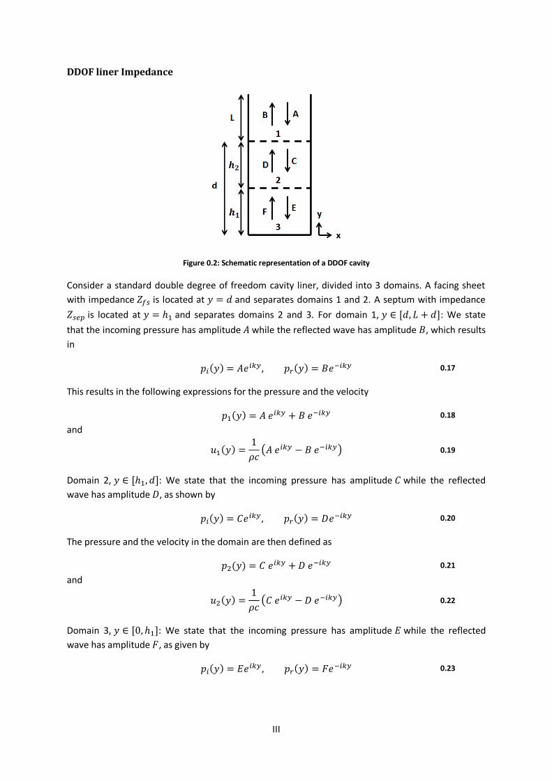
DDOF liner Impedance .............................................................................................................. III
Appendix B – COMSOL Tutorial for Baseline Folded Cavity Liner ..................................................... VI
v
Table of symbols and definitions
Symbol Description SI Unit
Acoustic admittance
Average acoustic Admittance
Sound Intensity of the incoming wave Sound Intensity of the reflected wave Length of the air column (to simulate impedance tube) Non – dimensional Resistance
Average non – dimensional Resistance
Non – dimensional Resistance of the folded cavity liner Non – dimensional Resistance of the facing sheet
Non – dimensional Resistance of the septum
Surface area Sound Pressure Level Acoustic impedance
Average acoustic impedance
Mechanical impedance of the facing sheet
Acoustic Impedance on the surface Mechanical impedance of the septum
Speed of sound Depth of the cavity Frequency
Frequency at maximal absorption Resonance Frequency Height of the cavity Height of the cavity Height of the neck Imaginary unit Wave number Length of the cavity
Mass inertance
Acoustic pressure
Amplitude of inlet pressure Pressure of incident wave Pressure of reflected wave
Reference pressure
Pressure on the surface Time Particle velocity
Velocity of the incoming wave normal to the surface
Velocity of the reflected wave normal to the surface
Particle Velocity normal to the surface
Width of the liner neck Sound power of incoming wave Sound power of reflected wave
vi
Non- dimensional Reactance Average non- dimensional Reactance
Non- dimensional Reactance of the folded cavity liner Absorption coefficient Diffuse field absorption coefficient
Angle of the incident wave with respect to the normal
Wave length Fluid density Angular frequency
1
1 Introduction
The level of noise from commercial and private aircraft is limited by governmental regulations.
Airports, such as the Washington International airport at night, even impose more severe limits [1].
Turbomachinery noise is one of the major noise sources in a modern commercial turbofan aircraft.
It affects residents close to airports. This “environmental” or “community” noise of this type of
aircraft is mainly a concern when the aircraft takes off or lands, but it is rarely an issue during cruise.
Suppression of the noise within the engine ducts for both the inlet and the exhaust is necessary to
meet the regulated limits [1] [2].
The noise of an aircraft engine is composed of noise from different source mechanisms. These noise
sources normally consist of the turbofan, compressor, turbine and combustor but also of jet mixing,
as shown in Figure 1.1 for a modern High Bypass Ratio (HBR) turbofan engine. Of the noise sources
in an aircraft engine fan noise and jet noise are the biggest contributors at take-off, while fan noise
and airframe noise are the most important factors during the landing. Reducing fan noise is
therefore essential to bring the whole aircraft noise levels down [3] [4] [5].
Fan noise is generated at the fan, propagates to the forward arc through the intake and to the rear
arc through the bypass ducts after which it is radiated to the atmosphere. In order to reduce fan
noise, acoustic liners are placed within the engine duct. This acoustic treatment is designed to
mainly attenuate the frequencies important to community noise. The purpose of the liners is to
attenuate the fan noise while it propagates trough the ducts before being radiated out. Therefore
they are placed on the internal walls of the engine intake and bypass duct. There are two main types
of liners used in turbofan engines; Single Degree of Freedom (SDOF) and Double or Two Degrees of
Freedom (DDOF or 2DOF) liners. The acoustic performance of these liners depends strongly on the
cell depth. In order to absorb lower frequencies deeper cells are needed, which is not always
possible due to mechanical design constraints. A solution for this problem can be found in folding
the liner cells such that deep liner cells can be fitted into shallow spaces. The concept of folded
cavity liners has been developed at the Noise UTC (Rolls-Royce University Technology Centre in Gas
Turbine Noise, Institute of Sound and Vibration Research, University of Southampton) and their
acoustic design has been investigated in recent years [3] [4]. These liners have the ability to act like a
mixture of a deep and a shallow liner, due to their folded geometry. As a result the folded cavity
liner can effectively absorb both high and low frequencies.
In this report the acoustic behaviour of folded cavity liners is studied. It will start with some basic
background of acoustics for understanding the physics and making liner models. A commercial finite
element package software COMSOL Multiphysics was used for the analysis of acoustics of folded
cavity liners. The normal incidence acoustic impedance and absorption coefficients of the liner are
calculated by using COMSOL models. The COMSOL model is validated against measured data and
also against predications by another commercial finite element code Actran TM. The measured data
is obtained by the National Aerospace Laboratory of the Netherlands which is also known as
'Nationaal Lucht- en Ruimtevaartlaboratorium' or NLR. A number of parametric studies have been
conducted in order to get a better insight in the acoustic behaviour of a folded cavity liner.
2
Figure 1.1 Noise sources on a turbofan engine [5].
3
2 Pressure Acoustics concerning Liners This chapter gives the reader a quick glance in the fundamentals of acoustic propagation and the
basics of acoustic liner theory. The fundamental expressions for the one-dimensional acoustic
pressure field, the definition of the acoustic impedance and the different types of absorption
coefficients are introduced. The typical liners used in aeroengine ducts are explained and the
theoretic impedance for both will be given. Finally the concept of the folded cavity liner will be
introduced.
2.1 Plane wave propagation
2.1.1 Acoustic pressure field
Figure 2.1 Pressure waves propagating in a straight duct
Consider plane waves propagating in a straight duct along the - axis, resulting in a one-dimensional
plane wave field, as shown by Figure 2.1. The pressure wave propagates in the positive -
direction and has amplitude leading to the definition of . The
pressure wave propagates in the negative - direction, with amplitude and is therefore defined as
[6]. The acoustic pressure at a certain point is expressed as the
sum of the pressure of the incident wave and the pressure of the reflected wave given
by
2.1
Now assume that the wave is actually the wave entering the duct and that is the wave
that is reflected at the end of the duct. The total acoustic pressure is then given by
2.2
where and are the amplitudes of the incoming and reflected wave, respectively. is the radial
frequency in , the time in seconds and the wavenumber in ].
2.1.2 Acoustic Impedance
The acoustic impedance, in [ ], can be divided in a real and an imaginary part as is given by
2.3
where R is the non-dimensional resistive part and X is the non-dimensional reactive part of the
impedance, which are multiplied by the mass density in and the speed of sound in
. The resistance represents the energy loss of the acoustic wave that is converted into other
4
forms of energy, due to for instance viscous effects or wall vibrations. The reactance represents the
ability to convert kinetic into potential energy and potential into kinetic energy. This can be the
result of the expansion and compression of acoustic waves, in a compressible medium such as air [7].
The impedance at a certain point is generally defined as the ratio of pressure and particle velocity
as , where is given in and in /s]. In the current case, the impedance with the
velocity in the negative - direction is given by
2.4
An expression for the particle velocity can be obtained from the momentum equation as derived by
Euler for an inviscid, perfect gas without body forces which is given by equation 2.5 [5].
2.5
When assuming small perturbations and a mean flow that is equal to zero, we can linearise Eq. 2.5
into equation 2.6.
2.6
We divide equation 2.6 by and assume that, since we are dealing with a plane wave along the -
axis, the situation can be considered one – dimensional. This then results in
2.7
Solving equation 2.7 by integrating the expression for the pressure, as was given in equation 2.2,
over time results in
2.8
Substituting equation 2.2 in equation 2.8, results in the expression for the particle velocity as a
function of and as given by
2.9
By substituting , the relation between the wavenumber , the speed of sound and the
radial frequency , equation 2.9 becomes
2.10
Finally we obtain an expression for the acoustic impedance at a position by substituting the
expressions for the pressure and the velocity in equation 2.1. The result is given by
2.11
5
2.2 Local reactive Surface
2.2.1 Single – angle incidence absorption
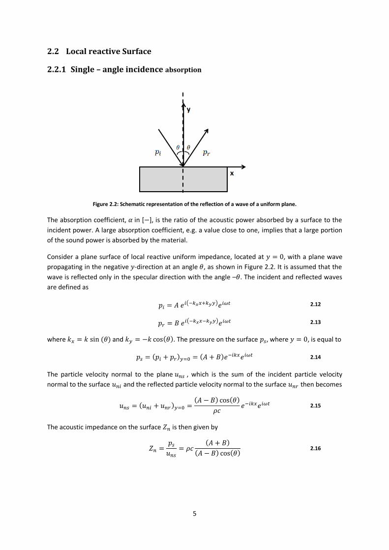
Figure 2.2: Schematic representation of the reflection of a wave of a uniform plane.
The absorption coefficient, in [ ], is the ratio of the acoustic power absorbed by a surface to the
incident power. A large absorption coefficient, e.g. a value close to one, implies that a large portion
of the sound power is absorbed by the material.
Consider a plane surface of local reactive uniform impedance, located at , with a plane wave
propagating in the negative -direction at an angle , as shown in Figure 2.2. It is assumed that the
wave is reflected only in the specular direction with the angle – . The incident and reflected waves
are defined as
2.12
2.13
where and . The pressure on the surface , where , is equal to
2.14
The particle velocity normal to the plane , which is the sum of the incident particle velocity
normal to the surface and the reflected particle velocity normal to the surface then becomes
2.15
The acoustic impedance on the surface is then given by
2.16
6
Rewriting equation 2.16 for the ration of the reflected and incident amplitude results in
2.17
The sound intensity is determined by the components normal to the wall. The intensity of the
incident and reflected wave are defined as
2.18
and
2.19
The sound power absorption coefficient is defined as the ratio between the power of the wave that
is not reflected and the power of the incident wave, as given by
2.20
Substituting equation 2.17 in equation 2.20 then gives the value for the absorption coefficient for a
plane wave with an incidence angle . This result is shown in equation 2.21 [8].
2.21
2.2.2 Normal incidence absorption
In the case of a propagating plane wave in an infinitely long duct, the angle of incidence can be
assumed to be zero. This particular case is called normal incidence absorption, for which the single-
incidence adsorption coefficient as given in equation 2.21 then reduces to
2.22
2.2.3 Diffuse field incidence
When the acoustic pressure waves are incident upon a boundary from all directions, we speak of a
diffuse field incidence [9]. The absorption coefficient in such a field is modelled by integrating
over all possible incidence angles, as is shown in equation 2.23 [8].
2.23
therefore
2.24
where
2.25
7
2.3 Acoustic liners in turbofan engine ducts
2.3.1 SDOF and DDOF liners
Figure 2.3: Construction of SDOF and DDOF acoustic liners [3]
A Single Degree of Freedom (SDOF) liner consists of a perforated facing sheet backed by a single
layer of honeycomb cells with a solid backing plate. In the case of Double Degree of Freedom (DDOF)
liners, there is an extra honeycomb layer which is separated from the other one by a porous septum
sheet. Schematic representations of a SDOF and a DDOF liner can be found in Figure 2.3 [3] [4].
There are two main benefits of introducing a septum. The resistance of the liner is controlled by the
septum rather than by the facing sheet, resulting in liners that are practically independent of duct
flow effects. Furthermore the resistance and reactance over a specific range of frequencies can be
better controlled. However, the facing sheet resistance must be small to achieve this [1].
The impedance of these two models can be obtained analytically from one-dimensional models. The
analytical impedance of a SDOF liner is given by
2.26
where is the impedance of the facing sheet, the wavenumber of an acoustic wave at
frequency and is the liner depth. The analytical impedance of a DDOF liner is given by
2.27
where and denotes the impedance of the septum. The total cell depth is given by
with the lower and the upper cell depth [1]. Derivations for equations 2.26 and 2.27 can be
found in Appendix A – Impedance derivations.
The acoustic performance of liners depends strongly on the cell depth. In order to absorb lower
frequencies a larger cell depth is needed, which is not always possible due to mechanical design
constraints. A solution for this problem can be found in folding the liner cells such that deep liner
cells can be fitted into shallow spaces, resulting in the so-called folded cavity liner.
8
2.3.2 Folded Cavity liners
Folded Cavity liners are L-shaped liners which can have just a facing sheet like the SDOF liner, but
can also exist with both a facing sheet and a septum like the DDOF liner. Their neck is generally filled
with honeycomb cells, but their cavity usually is not. Folded cavity liners have the ability to act like a
mixture of a deep and a shallow liner, due to their folded geometry.
Figure 2.4 and Figure 2.5 show the pressure distributions for a high and a low frequency pressure
wave. Higher frequencies will bounce of the back wall and experience a shallow liner, as is illustrated
in Figure 2.4. Lower frequencies on the other hand can propagate around the corner in order to fill
the entire cavity thereby experiencing a deep liner, as can be seen in Figure 2.5. As a result the
folded cavity liner can effectively absorb both high and low frequencies. As is illustrated in the
pressure plots of Figure 2.4 and Figure 2.5.
Figure 2.4 a folded cavity liner for high frequencies Figure 2.5 a folded cavity liner for low frequencies
9
3 COMSOL Modelling – Baseline Folded Cavity Liner This chapter explains step by step how the 2D COMSOL acoustic pressure model for a folded cavity is
made. It will start with a short problem description, after which all parameters choices are summed
up. The geometry, choice of mesh size will be explained, as well as the list of variables that are
defined in order to calculate the absorption coefficients and the acoustic impedance. A detailed
tutorial for this folded cavity liner COMSOL model can be found in Appendix B – COMSOL Tutorial for
Baseline Folded Cavity Liner.
3.1 Problem description and Validity In Figure 3.1 a schematic representation of a folded cavity liner is shown as a dark grey L – shaped
figure. It consists of a cavity with a neck on top. The neck is filled with honeycomb cells, which are
here represented by 5 rectangles. The folded cavity liner has a depth , a cavity length , a neck
width and a cavity height . The lighter grey object on top of the liner represents the air column
which has a length . The liner and the air column are separated by a facing sheet located at .
At there is a septum located that separates the neck and the cavity of the liner. At the inlet,
where , there is an incident plane wave propagating in the negative -direction and a
resulting reflected wave propagating in the positive - direction. If the liner has good absorption
the reflected wave as a result will be small.
The COMSOL model is basically a long duct with an interior impedance tube with a degree angle
at the end. At the inlet there is a plane wave imposed that propagates in the negative direction
trough the facing sheet and septum. At the back wall of the cavity, where , the pressure wave
is forced to go around the corner. This discontinuity results in scattering of the pressure waves and
occurrence of higher modes. The cut-off frequency in a duct is the frequency for which higher modes
start to cut on. This occurs when the width of the column is larger than roughly half a wavelength.
When the air column is wider than half a wavelength, the reflected wave will contain higher order
modes that propagate towards the inlet and influence the pressure predictions. As a result the
predictions for columns that are wider than half a wavelength are not accurate anymore.
Figure 3.1: Schematic representation of a folded cavity liner
10
3.2 COMSOL Model
3.2.1 Global Parameters
The first step in building a folded cavity model in COMSOL is defining some constants that consider
the geometry, the properties of the facing sheet, the amplitude of the incoming wave and the speed
of sound in air. The latter is needed, since the material property , which is predefined in
COMSOL, gives a local value and therefore cannot be used in global calculations. All these
parameters can be found in Table 3.1. The properties that are listed are the properties of the
standard folded cavity that is used throughout the entire study and it will be explicitly mentioned if
any of these constants differs.
COMSOL has predefined values of the density and the speed of sound for air. These values can be
found in Table 3.2.
Table 3.1 Parameters used in modelling the folded cavity in COMSOL
Name Expression Value Description
65[mm] 0.065000 m Height of cavity 200[mm] 0.200000 m Length of air column 50[mm] 0.050000 m Width of cavity/air column 2[mm] 0.0020000 m Mass inertance
1.05 1.050000 Resistance of facing sheet
2.05 2.050000 Resistance of septum
1[Pa] 1.0000 Pa Amplitude of incoming wave 343[m/s] 343.00 m/s Speed of sound (air)
Table 3.2: COMSOL default values for air
COMSOL Values for air
1.204 343.2
3.2.2 Geometry, pressure acoustics and meshes
a) Geometry b) Mesh
Figure 3.2: Geometry and mesh of the folded cavity liner
11
The folded cavity liner as depicted in Figure 3.2 a) has a liner depth of mm, a cavity length of
mm, a width of mm, a height of mm and an air column length of mm. It is important to
have a relatively long air column ( ) in the model in order ensure the validity of the plane wave
theory. The honeycomb cells located in the neck of the liner are modelled with a width of mm
and a height of mm. All the domains of the folded cavity liner are modelled with air and have,
with exception of the inlet, the facing sheet and septum, sound hard boundaries.
The facing sheet, located at the boundary between the air column and the neck at is modelled
with an interior impedance with a value of . The septum, located
at the boundary between the neck and the cavity at is modelled with an interior impedance
with a value of . The honeycomb cells, located in the neck, are
modelled with interior sound hard boundaries. At the inlet a plane wave radiation is defined, with an
incidence pressure field of type plane wave and an amplitude of incidence wave equal to . The
initial values for and are kept equal to zero.
The elements used are Lagrange Quadratic (default) Free Quadrilateral Elements, with a maximum
element size of 8 mm. This corresponds to a minimum of 7 elements per wavelength for frequencies
up to kHz, since , for is and is . The minimum element
size, maximum element growth rate, resolution of curvature and the resolution of narrow regions
are chosen to be , , and respectively, but have no large influence on the outcome
since this is a rather simple geometry. The mesh can be seen in Figure 3.2 b).
All results are obtained for by taking a frequency range starting from Hz to Hz, with a step
size of Hz, unless denoted otherwise. Though the maximum frequency might sometimes be
or Hz instead of the Hz mentioned here, the step size is Hz in general.
3.2.3 Derivation of the COMSOL expressions
3.2.3.1 Impedance
Recall that the acoustic impedance at the facing sheet located at , is given by equation 2.11:
3.1
Unfortunately the amplitudes of the incoming and outgoing waves cannot be measured at point
. Therefore the expression for the impedance at the facing sheet needs to be slightly altered.
Assuming that the amplitude of the incoming wave has a known value, which will from now on be
referred to as , and that the total pressure at the inlet is known from measurement. By
combining and we can now rewrite the pressure of
the incoming and reflected waves at the inlet as
3.2
and
3.3
therefore
3.4
12
We now have expressions for the total pressure, the incoming pressure wave and the reflected
pressure wave at the inlet. We can now use these to calculate the values of the pressure and the
velocity at the facing sheet. We do so by rewriting the exponentials into the following expressions:
3.5
and
3.6
Substituting these expressions in equation 3.1 results in
3.7
Multiplying both the numerator and the denominator by gives
3.8
Since and are known, we can now use this equation to calculate the impedance on the
facing sheet.
3.2.3.2 Absorption coefficients
Recall from the previous chapter that the acoustic impedance can be separated in a real and an
imaginary part and that the normal incidence absorption coefficient can be expressed into terms of
resistance and reactance as is given by equation 2.21. This normal incidence absorption coefficient
can also be obtained numerically by evaluating the ratio between the incident and reflected power
in COMSOL, as given by equation 3.9 [8].
3.9
When considering the relationship between the total pressure and the pressure of the ingoing and
reflected wave, the power of the waves and can then be expressed as
3.10
with, , the surface area of the inlet. The term is needed in the COMSOL Program to make up
for the phase difference at inlet. The diffusive field incidence absorption coefficient is calculated
from the acoustic impedance, as was given by equations 2.24 and 2.25.
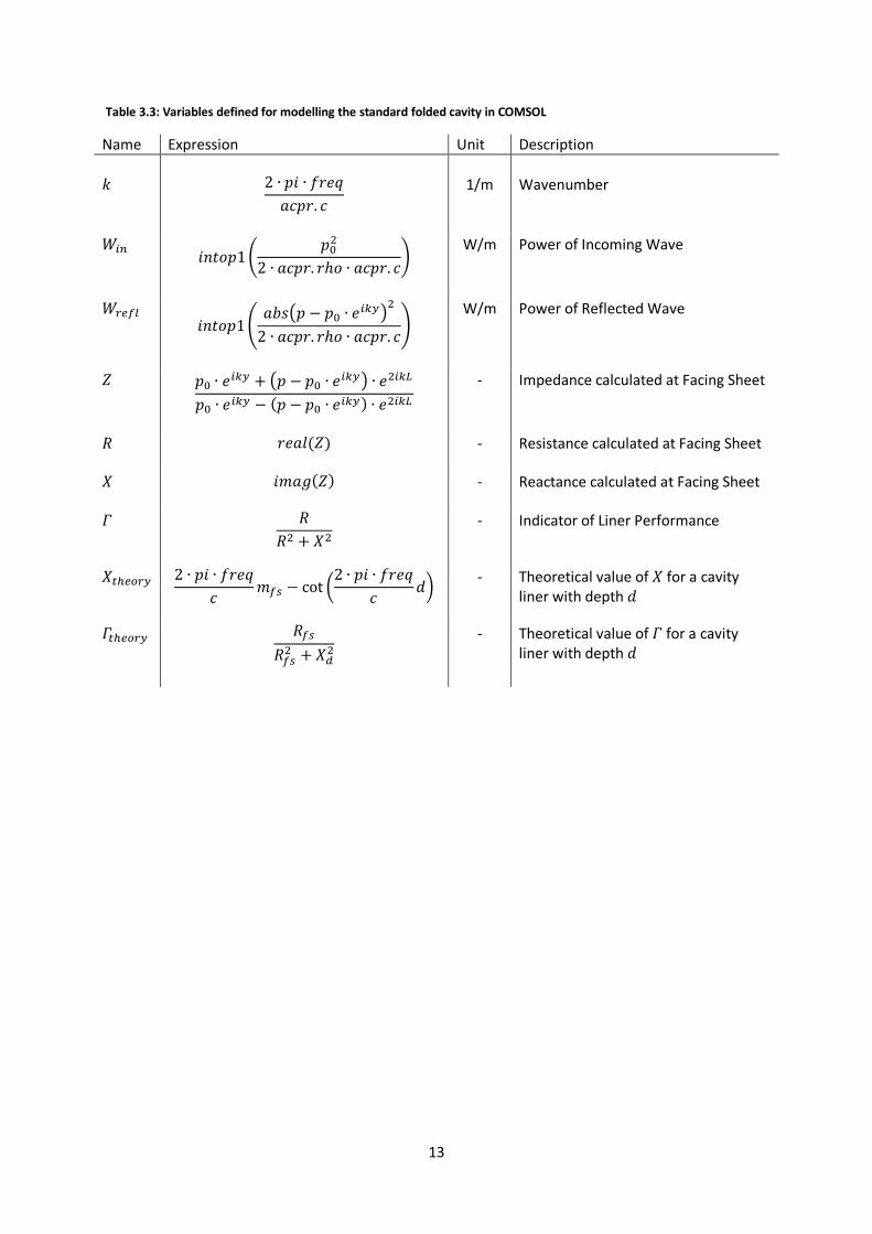
3.2.4 Variables
In order to help calculate the absorption coefficient and the impedance I defined some variables,
which can be found in Table 3.3. The term indicates a surface integral over the inlet, while
represents the local density of air as defined by COMSOL and the local speed of
sound in air as defined by COMSOL. COMSOL already has a predefined variable that
corresponds to the frequency of the pressure wave.
13
Table 3.3: Variables defined for modelling the standard folded cavity in COMSOL
Name Expression Unit Description
1/m
Wavenumber
W/m Power of Incoming Wave
W/m Power of Reflected Wave
- Impedance calculated at Facing Sheet
- Resistance calculated at Facing Sheet
- Reactance calculated at Facing Sheet
- Indicator of Liner Performance
- Theoretical value of for a cavity liner with depth
- Theoretical value of for a cavity liner with depth
14
4 Validation Studies These studies are performed to validate the use of a 2D COMSOL model as a good indication of liner
performance. By comparing the 2D folded cavity liner model with a 3D COMSOL model, we can check
whether the assumption that the 3rd dimension does not result in any major differences in results is
correct. Validation of the 2D could save a lot of time, since the modelling of an extra dimension can
result in a significant increase in computational time. We are also interested in the pressure
distribution within the liner cavity and we will compare this pressure predicted by COMSOL with
measured data from the NLR, the National Aerospace Laboratory of the Netherlands, and Actran
predictions. Finally we will compare the predictions of COMSOL for the impedance and absorption
coefficient for a folded cavity liner, with predictions made by Actran.
4.1 Model Descriptions
4.1.1 3D model
The geometry of the 3D model which is used to compare with the standard 2D model is shown in
Figure 4.1. The length in the -direction is chosen to be equal to the width of the liner neck which
corresponds to mm. The honeycomb cells now have a dimension of mm mm mm
, which means there now fit 25 cells between the septum and the facing sheet. Just as for
the 2D case the vertical walls of the honeycomb cells have been modelled with the option ‘Interior
Sound Hard Boundary (Wall)’ in the COMSOL ‘Pressure Acoustics’ menu. The values of the facing
sheet and the septum are identical to that of the 2D case.
For the mesh there is chosen to use Lagrange Quadratic (default) Free Tetrahedral Elements with a
maximum size of 9.28 mm. This is consistent with the default COMSOL extra fine mesh for this
geometry. This corresponds to approximately 6 elements per wavelength, for the highest frequency
of kHz at a speed of sound in air of . The study is performed for frequencies between
and Hz with steps of Hz. For this study the septum has been removed from both the
2D and the 3D model.
Figure 4.1 The 3D folded cavity with honeycomb cells
4.1.2 COMSOL Pressure Distribution
To get a good insight of what happens within the cavity of a folded cavity liner after sending in a
plane wave, we can look at the pressure distributions for different frequencies. The pressures values
are visualised by Sound Pressure Level (SPL) values that are referenced by a reference sound
15
pressure in air of Pa. This is value is considered to be the threshold of human
hearing (at kHz). The SPL is related to the pressure and is defined as is given by equation 4.1 [8]
4.1
4.1.3 Pressure Measurements Measured data
Figure 4.2 Placing of the microphones
During the NLR pressure tests 4 microphones were placed: one in the facing sheet, one in the
septum, one in the back wall and one in the side wall, as is shown by the red dots in Figure 4.2. The
microphone of the septum was still present in the case that there was no septum layer. The data of
the pressure measurements of the NLR and Actran predictions have been taken from the “Folded
Cavity Liner NLR test report” of 20 October 2011 by Paul Murray of the ISVR [10]. The measurements
were conducted for 3 different septum conditions: no septum, a low resistance septum and a high
resistance septum.
The value of the facing sheet resistance used in the NLR test was measured to be , while
the low resistance septum’s resistance corresponds to and the high resistance septum was
measured to have a value of . The same values are used in the COMSOL model. The mass
inertance of the sheets was taken as a constant, at m. Resulting in a reactance that varies
with frequency, as is given by , where is the wavenumber.
In the COMSOL model, the values of the pressure are extracted trough data points, located at the
same spots as the microphones in the NLR test model. It must be noticed that the microphone of the
facing sheet and the septum measured the pressure just above the resistive sheet. Therefore the
data points of these two locations are chosen to be mm above the exact location of the facing
sheet and the septum in order to match the measurements of the NLR.
4.1.4 Actran Model
The Actran Model has the same geometry as the standard folded cavity liner that was modelled in
COMSOL. The impedance of the facing sheet and the septum are equal as well. The main difference
between the COMSOL model and the Actran model is that the Actran model has no problems with
the influence of higher modes on the pressure predictions. This is due to the fact that only the plane
wave mode of the reflected wave is considered for the pressure predictions, as a result of the
16
anechoic boundary condition. Therefore the Actran predictions are not influenced by the width of
the air column, while those of COMSOL are. For that reason COMSOL and Actran might differ for
widths larger than half a wavelength. The Actran data, used in this report, has been used in
AIAA/CEAS Aeroacoustics Conference of 2012 [3] and was obtained by R. Sugimoto.
4.2 Results
4.2.1 2D V.S. 3D
As mentioned before the results for the 2D case are obtained by taking steps of Hz, while for the
3D the steps are Hz instead. This is chosen in order to save computational time, while still
allowing the reader to observe whether or not there is a good match between the 2D data and the
3D data. Frequencies higher than the cut-off frequency, which is around kHz for this liner, are
examined as well. In chapter 5.2 we will be looking into the geometry en resistance values of the
facing sheet and septum and behaviour they have on the impedance and diffuse field absorption
field curves. For now we just look at the differences between the 2D and the 3D COMSOL model.
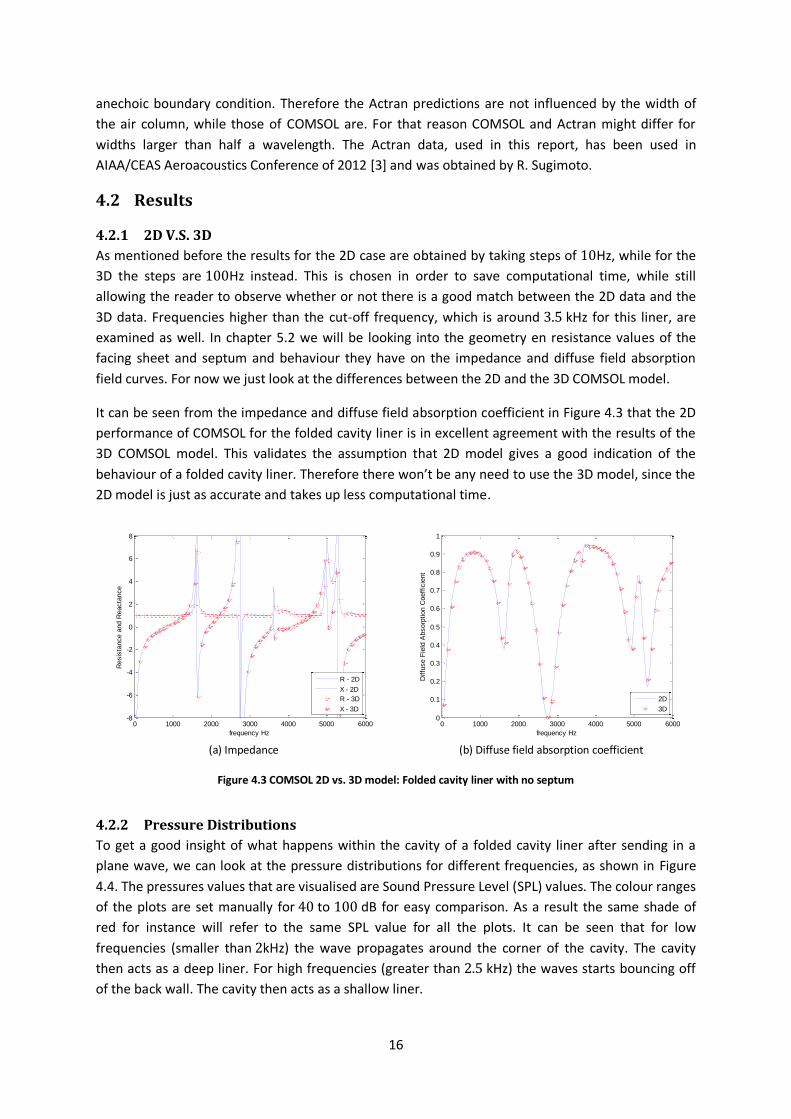
It can be seen from the impedance and diffuse field absorption coefficient in Figure 4.3 that the 2D
performance of COMSOL for the folded cavity liner is in excellent agreement with the results of the
3D COMSOL model. This validates the assumption that 2D model gives a good indication of the
behaviour of a folded cavity liner. Therefore there won’t be any need to use the 3D model, since the
2D model is just as accurate and takes up less computational time.
(a) Impedance (b) Diffuse field absorption coefficient
Figure 4.3 COMSOL 2D vs. 3D model: Folded cavity liner with no septum
4.2.2 Pressure Distributions
To get a good insight of what happens within the cavity of a folded cavity liner after sending in a
plane wave, we can look at the pressure distributions for different frequencies, as shown in Figure
4.4. The pressures values that are visualised are Sound Pressure Level (SPL) values. The colour ranges
of the plots are set manually for to dB for easy comparison. As a result the same shade of
red for instance will refer to the same SPL value for all the plots. It can be seen that for low
frequencies (smaller than kHz) the wave propagates around the corner of the cavity. The cavity
then acts as a deep liner. For high frequencies (greater than kHz) the waves starts bouncing off
of the back wall. The cavity then acts as a shallow liner.
0 1000 2000 3000 4000 5000 6000-8
-6
-4
-2
0
2
4
6
8
frequency Hz
Resis
tance a
nd R
eacta
nce
R - 2D
X - 2D
R - 3D
X - 3D
0 1000 2000 3000 4000 5000 60000
0.1
0.2
0.3
0.4
0.5
0.6
0.7
0.8
0.9
1
frequency Hz
Diffu
se F
ield
Absorp
tion C
oeff
icie
nt
2D
3D
17
SPL, F=500 Hz SPL, F=1000 Hz
SPL, F=1250 Hz SPL, F=1500 Hz
SPL, F=1750 Hz SPL, F=2000 Hz
SPL, F=2500 Hz SPL, F=3000 Hz
Figure 4.4 SPLs for the no septum case
18
4.2.3 Pressure Predictions
4.2.3.1 COMSOL vs. Measurements
a) Facing sheet (+0.1mm) as reference b) Back wall as reference
c) Facing sheet (+0.1mm) as reference d) Back wall as reference
e) Facing sheet (+0.1mm) as reference f) Back wall as reference
Figure 4.5 Comparison COMSOL and measured data NLR
0 500 1000 1500 2000 2500 3000-45
-40
-35
-30
-25
-20
-15
-10
-5
0
5
Frequency (Hz)
Sound P
ressure
Level (d
B)
No Septum
Facing sheet
Septum
Side Wall
Back Wall
0 500 1000 1500 2000 2500 3000-50
-40
-30
-20
-10
0
10
20
30
40
Frequency (Hz)
Sound P
ressure
Level (d
B)
No Septum
Facing sheet
Septum
Side Wall
Back Wall
0 500 1000 1500 2000 2500 3000-35
-30
-25
-20
-15
-10
-5
0
5
Frequency (Hz)
Sound P
ressure
Level (d
B)
0.6 c Septum
Facing sheet
Septum
Side Wall
Back Wall
0 500 1000 1500 2000 2500 3000-20
-10
0
10
20
30
40
Frequency (Hz)
Sound P
ressure
Level (d
B)
0.6 c Septum
Facing sheet
Septum
Side Wall
Back Wall
0 500 1000 1500 2000 2500 3000-45
-40
-35
-30
-25
-20
-15
-10
-5
0
5
Frequency (Hz)
Sound P
ressure
Level (d
B)
2.05 c Septum
Facing sheet
Septum
Side Wall
Back Wall
0 500 1000 1500 2000 2500 3000-20
-10
0
10
20
30
40
50
Frequency (Hz)
Sound P
ressure
Level (d
B)
2.05 c Septum
Facing sheet
Septum
Side Wall
Back Wall
19
We want to know how accurate the pressure predictions throughout the liner cavity are compared
to values obtained during pressure measurements with a testing model at the NLR. We therefore
compare the pressure at 4 important locations in the cavity: at the facing sheet, at the septum, at
the back wall and at the side wall.
Since the exact conditions for the NLR measurements are impossible to reproduce, we have chosen
to reference all SPL values to the results of one of the microphones/data points. First all the NLR
data is referenced to the data of the facing sheet measurements, while the COMSOL data is
referenced to the data from the data point just above the facing sheet. In this way, the differences
between the two facing sheets itself cannot be determined, but by looking at the absolute pressure
differences between the facing sheet and the other points we can see how accurate the rest of the
data obtained by COMSOL is. To see the difference between the COMSOL data of the facing sheet
and the NLR data of the facing sheet, we decided to investigate a second case in which all results are
referenced to the back wall. The results for both cases, for different septum resistances, can be
found in Figure 4.5. The continuous lines are the COMSOL data and the stars are the measured data.
It can be seen from the data at the first measurement point, which corresponds to 160 Hz, that the
differences between the COMSOL data and the pressure measurements of the NLR differ about 8 dB,
which is quite a lot. However for higher frequencies the results prove pretty accurate. It can be seen
that when looking at the plots referenced to the facing sheet that the septum predictions are really
accurate, while for the plots referenced to the back wall, the results of the side wall are better. This
might be due to the fact that the facing sheet and the septum are both modelled with interior
impedance boundaries, while the side and the back wall both have solid wall boundaries.
4.2.3.2 COMSOL vs. Actran
Figure 4.6 shows the SPLs as calculated by both the COMSOL and the Actran models, both
referenced with respect to the facing sheet. The continuous line is the COMSOL data, while the
diamonds represent the Actran data. The blue line represents the facing sheet, the green one is the
septum, the red one the side wall and the black one represents the back wall, for which there are no
Actran predictions made. As can be seen, the data of the pressure at the facing sheet, the septum,
the side wall and the back wall of the COMSOL and the Actran models are nearly identical. It can be
seen that the agreement between the two increases as the resistance of the septum increases. This
is due to the dampening effect of the septum that ensures that the pressure in the neck of the liner
is more continuous. Below the cut-off frequency where the higher modes start to cut- on the
COMSOL predictions are just as accurate as those made by Actran.
a) No Septum b) Low resistance septum c) High resistance septum
Figure 4.6 SPL comparison between COMSOL and Actran
0 500 1000 1500 2000 2500 3000-40
-35
-30
-25
-20
-15
-10
-5
0
5
Frequency (Hz)
Sound P
ressure
Level (d
B)
No Septum
Facing sheet
Septum
Side Wall
Back Wall
0 500 1000 1500 2000 2500 3000-35
-30
-25
-20
-15
-10
-5
0
5
Frequency (Hz)
Sound P
ressure
Level (d
B)
0.6 c Septum
Facing sheet
Septum
Side Wall
Back Wall
0 500 1000 1500 2000 2500 3000-45
-40
-35
-30
-25
-20
-15
-10
-5
0
5
Frequency (Hz)
Sound P
ressure
Level (d
B)
2.05 c Septum
Facing sheet
Septum
Side Wall
Back Wall
20
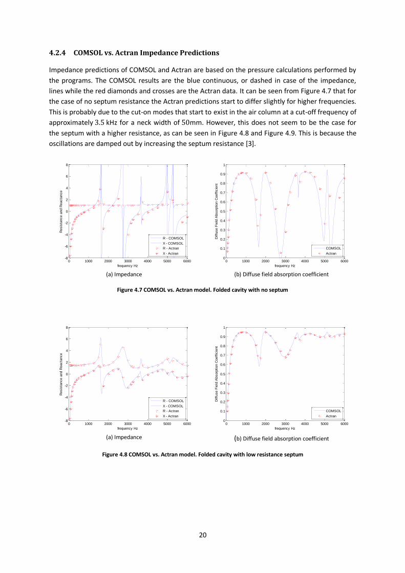
4.2.4 COMSOL vs. Actran Impedance Predictions
Impedance predictions of COMSOL and Actran are based on the pressure calculations performed by
the programs. The COMSOL results are the blue continuous, or dashed in case of the impedance,
lines while the red diamonds and crosses are the Actran data. It can be seen from Figure 4.7 that for
the case of no septum resistance the Actran predictions start to differ slightly for higher frequencies.
This is probably due to the cut-on modes that start to exist in the air column at a cut-off frequency of
approximately kHz for a neck width of mm. However, this does not seem to be the case for
the septum with a higher resistance, as can be seen in Figure 4.8 and Figure 4.9. This is because the
oscillations are damped out by increasing the septum resistance [3].
(a) Impedance (b) Diffuse field absorption coefficient
Figure 4.7 COMSOL vs. Actran model. Folded cavity with no septum
(a) Impedance (b) Diffuse field absorption coefficient
Figure 4.8 COMSOL vs. Actran model. Folded cavity with low resistance septum
0 1000 2000 3000 4000 5000 6000-8
-6
-4
-2
0
2
4
6
8
frequency Hz
Resis
tance a
nd R
eacta
nce
R - COMSOL
X - COMSOL
R - Actran
X - Actran
0 1000 2000 3000 4000 5000 60000
0.1
0.2
0.3
0.4
0.5
0.6
0.7
0.8
0.9
1
frequency Hz
Diffu
se F
ield
Absorp
tion C
oeff
icie
nt
COMSOL
Actran
0 1000 2000 3000 4000 5000 6000-8
-6
-4
-2
0
2
4
6
8
frequency Hz
Resis
tance a
nd R
eacta
nce
R - COMSOL
X - COMSOL
R - Actran
X - Actran
0 1000 2000 3000 4000 5000 60000
0.1
0.2
0.3
0.4
0.5
0.6
0.7
0.8
0.9
1
frequency Hz
Diffu
se F
ield
Absorp
tion C
oeff
icie
nt
COMSOL
Actran
21
(a) Impedance (b) Diffuse field absorption coefficient
Figure 4.9 COMSOL vs. Actran model. Folded cavity with high resistance septum
4.3 Conclusion It was shown that the 2D COMSOL liner model can predict the pressure, impedance and absorption
coefficients just as accurate as a 3D COMSOL can, for a square liner neck. The knowledge that the
third dimension of a liner model can be neglected can save up a lot of computational time in the
future.
It was shown that for frequencies up to the cut-off frequency the COMSOL models predictions are
just as good as those of the Actran model and come pretty close to those of the NLR measurements.
Therefore it is concluded that the COMSOL model is a good approximation of the reality and can be
used to predict the behaviour of folded cavity liners effectively.
0 1000 2000 3000 4000 5000 6000-8
-6
-4
-2
0
2
4
6
8
frequency Hz
Resis
tance a
nd R
eacta
nce
R - COMSOL
X - COMSOL
R - Actran
X - Actran
0 1000 2000 3000 4000 5000 60000
0.1
0.2
0.3
0.4
0.5
0.6
0.7
0.8
0.9
1
frequency Hz
Diffu
se F
ield
Absorp
tion C
oeff
icie
nt
COMSOL
Actran
22
5 Parametric Studies In the first three parametric studies we examine the influence of the geometry on liner performance.
We vary the length, the height and the width of the cavity and compare the results. For the second
part of the parametric studies we examine the influence of the resistances of the facing sheet, the
septum and the placement of a second septum on the performance of the liner. As mentioned before
we used the standard cavity liner, as is described in Chapter 2, as a default.
5.1 Geometry and Resistances
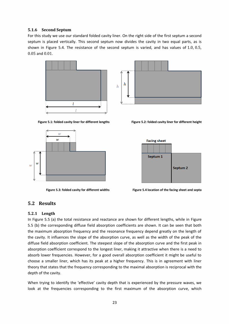
5.1.1 Length
The cavity length is defined as the distance from one side wall to another, as is shown in Figure 5.1.
The effect of the length of the cavity on the geometry of the liner is examined by changing the
length of the cavity, while keeping width of the column the same. The thick dark lines in the figure
depict an example of a changed geometry, while the reference geometry is in grey.
5.1.2 Height
The cavity height is here defined to be the distance from septum to the back wall of the cavity, as
can be seen in Figure 5.2. The effect of the height of the cavity on the geometry of the liner can be
investigated by changing the height, but by keeping the length and width of the air column constant.
The thick dark lines depict an example of a change in the geometry, as a result of a change in the
height.
5.1.3 Width
The cavity width is defined as both the height of the cavity and the width of the neck of the liner.
The result is a folded column with constant width, as is shown in Figure 5.3. The effect of the width
of the liner can be seen when the width is changed, but length of the cavity remains the same. The
thick dark lines depict an example of a changed geometry, while the reference geometry is in grey.
5.1.4 Facing sheet
The location of the facing sheet can be found in Figure 5.4. The acoustic impedance of the facing
sheet is defined as . While remaining a constant geometry and septum resistance,
the influence of the facing sheet resistance on the total impedance and the absorption coefficient
was examined by using three different values: (a) a high resistance facing sheet , (b) a
medium resistance facing sheet and a low resistance facing sheet ( ). In all
three cases the mass inertance of the facing sheet is m. The resistance of the septum
remained at a constant value during this study; and the mass inertance was equal to
that of the facing sheet.
5.1.5 Septum
The location of the septum can be found in Figure 5.4. While remaining a constant geometry and
facing sheet resistance, the influence of the septum resistance on the total impedance and the
absorption coefficient was examined by using three different values: (a) a high resistance septum
, (b) a low resistance septum and (c) no septum. The mass inertance of
the septum is m. The resistance of the facing sheet remained at a constant value during
this study; and the mass inertance was equal to that of the septum, m.
23
5.1.6 Second Septum
For this study we use our standard folded cavity liner. On the right side of the first septum a second
septum is placed vertically. This second septum now divides the cavity in two equal parts, as is
shown in Figure 5.4. The resistance of the second septum is varied, and has values of , ,
and .
Figure 5.1: folded cavity liner for different lengths Figure 5.2: folded cavity liner for different height
Figure 5.3: folded cavity for different widths Figure 5.4 location of the facing sheet and septa
5.2 Results
5.2.1 Length
In Figure 5.5 (a) the total resistance and reactance are shown for different lengths, while in Figure
5.5 (b) the corresponding diffuse field absorption coefficients are shown. It can be seen that both
the maximum absorption frequency and the resonance frequency depend greatly on the length of
the cavity. It influences the slope of the absorption curve, as well as the width of the peak of the
diffuse field absorption coefficient. The steepest slope of the absorption curve and the first peak in
absorption coefficient correspond to the longest liner, making it attractive when there is a need to
absorb lower frequencies. However, for a good overall absorption coefficient it might be useful to
choose a smaller liner, which has its peak at a higher frequency. This is in agreement with liner
theory that states that the frequency corresponding to the maximal absorption is reciprocal with the
depth of the cavity.
When trying to identify the ‘effective’ cavity depth that is experienced by the pressure waves, we
look at the frequencies corresponding to the first maximum of the absorption curve, which
24
corresponds to a quarter of the wavelength and the first resonance frequency, which corresponds to
half a wavelength. The latter can also be considered as the minimum absorption frequency. In Table
5.1 these resonance frequencies are listed, along with the effective cavity length as experienced by
the pressure waves, calculated from . It can be seen that liner length and the effective
length correspond quite well, considering the fact that for frequencies around Hz the step size of
Hz can results in errors of approximately mm.
In Table 5.2 the frequencies corresponding to the first maximum of the absorption curve are listed,
along with the effective cavity length as experienced by the pressure waves, calculated from
. As was expected the effective length increases when the length increases.
Moreover, it can be seen that the effective length corresponds nicely to the actual length of the
cavity, with an exception for mm. This deviation might be due to the fact that the absorption
peak is very broad, so a small error in the solution can cause a significant shift in the maximum
absorption.
(a) Impedance (b) Diffuse field absorption coefficient
Figure 5.5 Folded Cavity with different lengths
Table 5.1 First resonance frequency for different lengths
Cavity length [mm]
Frequency [Hz]
Effective length [mm] Table 5.2 First maximal absorption for different lengths
Cavity length [mm]
Frequency [Hz]
Effective length [mm]
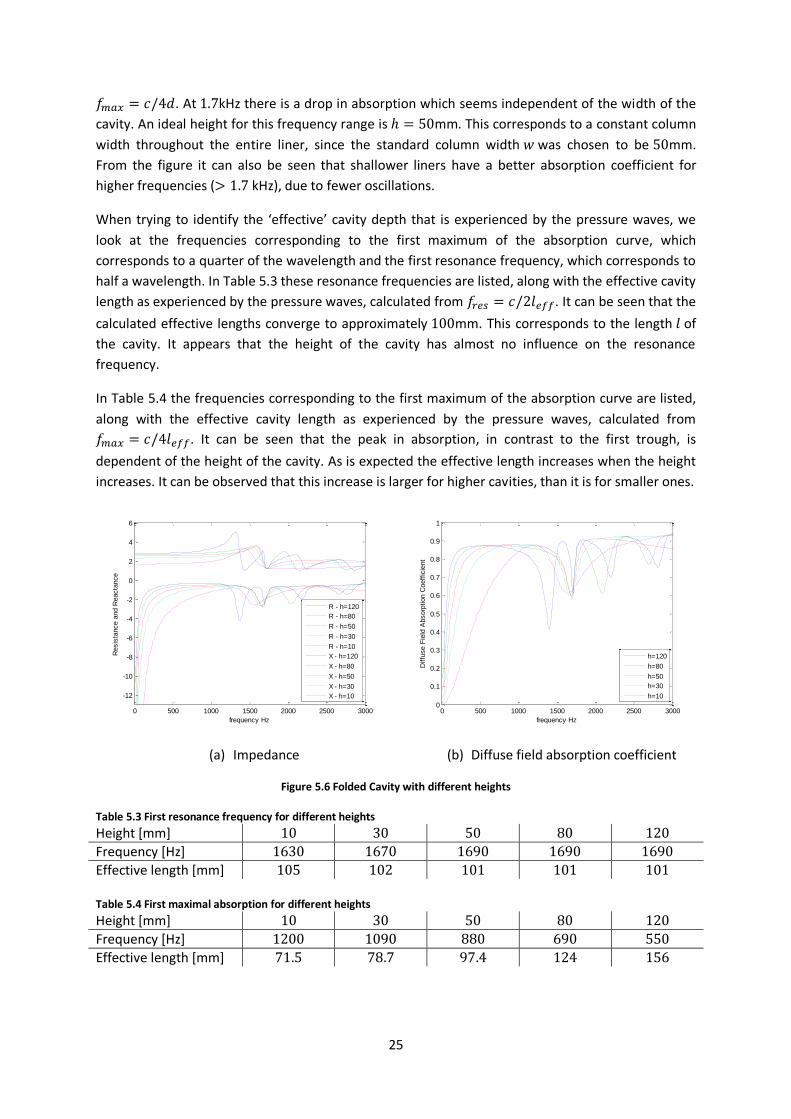
5.2.2 Height
In Figure 5.6 (a) the total resistance and reactance are shown for different heights, while in Figure
5.6 (b) the diffuse field absorption coefficient is shown. It can be seen that deeper liners exhibit
better absorption behaviour than shallower liners for frequencies up to kHz. This is visible by a
steeper slope and a wider peak in the absorption. This observation corresponds with liner theory
that states that the maximum absorption frequency is inversely dependent to the liner depth
0 500 1000 1500 2000 2500 3000
-15
-10
-5
0
5
10
frequency Hz
Resis
tance a
nd R
eacta
nce
R - l=60
R - l=80
R - l=100
R - l=150
R - l=210
X - l=60
X - l=80
X - l=100
X - l=150
X - l=210
0 500 1000 1500 2000 2500 30000
0.1
0.2
0.3
0.4
0.5
0.6
0.7
0.8
0.9
1
frequency Hz
Diffu
se F
ield
Absorp
tion C
oeff
icie
nt
l=60
l=80
l=100
l=150
l=210
25
. At kHz there is a drop in absorption which seems independent of the width of the
cavity. An ideal height for this frequency range is mm. This corresponds to a constant column
width throughout the entire liner, since the standard column width was chosen to be mm.
From the figure it can also be seen that shallower liners have a better absorption coefficient for
higher frequencies ( kHz), due to fewer oscillations.
When trying to identify the ‘effective’ cavity depth that is experienced by the pressure waves, we
look at the frequencies corresponding to the first maximum of the absorption curve, which
corresponds to a quarter of the wavelength and the first resonance frequency, which corresponds to
half a wavelength. In Table 5.3 these resonance frequencies are listed, along with the effective cavity
length as experienced by the pressure waves, calculated from . It can be seen that the
calculated effective lengths converge to approximately mm. This corresponds to the length of
the cavity. It appears that the height of the cavity has almost no influence on the resonance
frequency.
In Table 5.4 the frequencies corresponding to the first maximum of the absorption curve are listed,
along with the effective cavity length as experienced by the pressure waves, calculated from
. It can be seen that the peak in absorption, in contrast to the first trough, is
dependent of the height of the cavity. As is expected the effective length increases when the height
increases. It can be observed that this increase is larger for higher cavities, than it is for smaller ones.
(a) Impedance (b) Diffuse field absorption coefficient
Figure 5.6 Folded Cavity with different heights
Table 5.3 First resonance frequency for different heights
Height [mm]
Frequency [Hz]
Effective length [mm] Table 5.4 First maximal absorption for different heights
Height [mm]
Frequency [Hz]
Effective length [mm]
0 500 1000 1500 2000 2500 3000
-12
-10
-8
-6
-4
-2
0
2
4
6
frequency Hz
Resis
tance a
nd R
eacta
nce
R - h=120
R - h=80
R - h=50
R - h=30
R - h=10
X - h=120
X - h=80
X - h=50
X - h=30
X - h=10
0 500 1000 1500 2000 2500 30000
0.1
0.2
0.3
0.4
0.5
0.6
0.7
0.8
0.9
1
frequency Hz
Diffu
se F
ield
Absorp
tion C
oeff
icie
nt
h=120
h=80
h=50
h=30
h=10
26
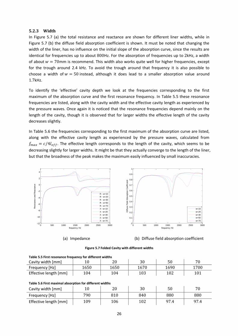
5.2.3 Width
In Figure 5.7 (a) the total resistance and reactance are shown for different liner widths, while in
Figure 5.7 (b) the diffuse field absorption coefficient is shown. It must be noted that changing the
width of the liner, has no influence on the initial slope of the absorption curve, since the results are
identical for frequencies up to about Hz. For the absorption of frequencies up to kHz, a width
of about mm is recommend. This width also works quite well for higher frequencies, except
for the trough around 2.4 kHz. To avoid the trough around that frequency it is also possible to
choose a width of instead, although it does lead to a smaller absorption value around
kHz.
To identify the ‘effective’ cavity depth we look at the frequencies corresponding to the first
maximum of the absorption curve and the first resonance frequency. In Table 5.5 these resonance
frequencies are listed, along with the cavity width and the effective cavity length as experienced by
the pressure waves. Once again it is noticed that the resonance frequencies depend mainly on the
length of the cavity, though it is observed that for larger widths the effective length of the cavity
decreases slightly.
In Table 5.6 the frequencies corresponding to the first maximum of the absorption curve are listed,
along with the effective cavity length as experienced by the pressure waves, calculated from
. The effective length corresponds to the length of the cavity, which seems to be
decreasing slightly for larger widths. It might be that they actually converge to the length of the liner,
but that the broadness of the peak makes the maximum easily influenced by small inaccuracies.
(a) Impedance (b) Diffuse field absorption coefficient
Figure 5.7 Folded Cavity with different widths
Table 5.5 First resonance frequency for different widths
Cavity width [mm]
Frequency [Hz]
Effective length [mm] Table 5.6 First maximal absorption for different widths
Cavity width [mm]
Frequency [Hz]
Effective length [mm]
0 500 1000 1500 2000 2500 3000-12
-10
-8
-6
-4
-2
0
2
4
frequency Hz
Resis
tance a
nd R
eacta
nce
R - w=10
R - w=20
R - w=30
R - w=50
R - w=70
X - w=10
X - w=20
X - w=30
X - w=50
X - w=70
0 500 1000 1500 2000 2500 30000
0.1
0.2
0.3
0.4
0.5
0.6
0.7
0.8
0.9
1
frequency Hz
Diffu
se F
ield
Absorp
tion C
oeff
icie
nt
w=10
w=20
w=30
w=50
w=70
27
5.2.4 Facing sheet
As can be seen in Figure 5.8 (a) adding to the resistance of the facing sheet, results in an increase
of the total resistance of 1.0. Just as increasing the resistance of the facing sheet with 0.5 results in
an increase of the total resistance of 0.5. However, a change in the values of the facing sheet
resistance has no influence on the total reactance. This observation would corresponds with
equation 2.27, that states that the total impedance is equal to the facing sheet impedance plus a
term that is constant for constant frequency, geometry and septum.
As can be seen in Figure 5.8 (b) results in the highest absorption at low frequencies, but
for noise reduction in the overall frequency domain, the is the better option. The
scores worse than either the or the on pretty much every frequency and is
therefore not recommended.
(a) Impedance (b) Diffusive Field Absorption Coefficient
Figure 5.8 Folded Cavity liner for different Facing Sheet resistances
5.2.5 Septum
(a) Impedance (b) Diffusive Field Absorption Coefficient
Figure 5.9 Folded Cavity liner for different Facing Sheet resistances
0 500 1000 1500 2000 2500 3000-10
-8
-6
-4
-2
0
2
4
6
frequency Hz
Resis
tance a
nd R
eacta
nce
R - Rf=2
X - Rf=2
R - Rf=1
X - Rf=1
R - Rf=0.5
X - Rf=0.5
0 500 1000 1500 2000 2500 30000
0.1
0.2
0.3
0.4
0.5
0.6
0.7
0.8
0.9
1
frequency Hz
Diffu
se F
ield
Absorp
tion C
oeff
icie
nt
Rf=2
Rf=1
Rf=0.5
0 500 1000 1500 2000 2500 3000-8
-6
-4
-2
0
2
4
6
8
frequency Hz
Resis
tance a
nd R
eacta
nce
R - Rs=2
X - Rs=2
R - Rs=0.6
X - Rs=0.6
R - Rs=0
X - Rs=0
0 500 1000 1500 2000 2500 30000
0.1
0.2
0.3
0.4
0.5
0.6
0.7
0.8
0.9
1
frequency Hz
Diffu
se F
ield
Absorp
tion C
oeff
icie
nt
Rs=2
Rs=0.6
Rs=0
28
The influence of increasing the septum resistance is not as straight forward as the influence of
increasing the resistance of the facing sheet. However it is clear from Figure 5.9 (a) that increasing
the septum resistance damps out the oscillations of the resistance and the reactance. From Figure
5.9 (b) it can be noted that the gives the highest absorption coefficient for low
frequencies, but for the case that the troughs in absorption are damped out best and
could therefore more effective for a broad range of frequencies.
5.2.6 Second Septum
In Figure 5.10 the impedances and the diffuse field absorption coefficients are given for the four
different second septum resistances. As expected it can be seen that a higher resistance decreases
the trough around kHz significantly, though it also decreases the peaks in absorption slight. A
value around is probably a good choice, since it significantly increases the absorption
coefficient at kHz, without losing to much performance around Hz.
a) Impedance b) Diffuse Field Absorption Coefficient
Figure 5.10 performance of the folded cavity liner for different resistance values of the second septum
5.3 Conclusion The length of the cavity has the biggest influence on the location of the maximum of the absorption
coefficient and the resonance frequency. As a result the width of the peak in absorption coefficient
can be regulated by the length of the cavity. The effective lengths calculated from the first trough
and peak in absorption are observed to match the actual length of the cavity well. The effective
length corresponding to the resonance frequency is slightly higher, while the effective length
corresponding to the maximal absorption is slightly lower than the actual length.
The height of the column has influence on the slope and the width of the first absorption peak.
Smaller heights give a better performance at high frequencies, while larger heights give a better
performance at low frequencies. The height has almost no influence on the resonance frequency,
where the diffuse field absorption coefficient is minimal. However, when the height of the cavity
increases it shifts the maximal absorption frequency to a lower frequency, resulting in an effective
length that is larger.
0 500 1000 1500 2000 2500 3000-12
-10
-8
-6
-4
-2
0
2
4
frequency Hz
Resis
tance a
nd R
eacta
nce
R - Rs2 = 1.0
R - Rs2 = 0.5
R - Rs2 = 0.05
R - Rs2 = 0.01
X - Rs2 = 1.0
X - Rs2 = 0.5
X - Rs2 = 0.05
X - Rs2 = 0.01
0 500 1000 1500 2000 2500 30000
0.1
0.2
0.3
0.4
0.5
0.6
0.7
0.8
0.9
1
frequency Hz
Diffu
se F
ield
Absorp
tion C
oeff
icie
nt
Rs2 = 1.0
Rs2 = 0.5
Rs2 = 0.05
Rs2 = 0.01
29
The width of the column has hardly any influence on frequencies up to Hz, though each width
has a distinctive curve for higher frequencies. The width appears to be the only parameter that
seems to have something of an optimal value, regardless of the desired frequency range. Changing
the width has hardly any influence on the effective lengths calculated from the maximal and minimal
absorption coefficient.
It is observed that the change in resistance of the facing sheet results in the same change in the total
acoustic resistance. For noise reduction that mainly involves low frequencies, it is better to
implement a facing sheet with a lower resistance. However, when one wants to reduce the noise on
a broad range of frequencies a facing sheet with a value close to might be the best option to
reduce the depth of the troughs. A high resistance facing sheet reduces the peak in the absorption
with a significant amount, in is therefore not recommended.
Variations in the resistance of the septum result in change in both the total resistance and reactance.
Higher septum resistance leads to a damping of the oscillations of the impedance. For noise
reduction one must consider what is preferred: a more constant absorption coefficient with a better
reduction of noise in the high frequencies or a more oscillating absorption coefficient which is
especially good at absorbing the low frequencies. In the first case a high septum resistance is
desirable, but in the second case the septum with a lower resistance is recommended.
It can be concluded from this study that placing a second septum can have a significant influence on
the performance of a folded cavity liner. It can be used to significantly decrease deep troughs at
unwanted locations and though it also affects the maximum absorption at some points, those losses
are only slight compared to the profit that can be made on other points.
30
6 Series of liners For efficient implementation of the liner, the folded cavity liner must be placed in series. However,
that will lead to unused space closed off by solid hard walls, which is bad for overall the liner
performance. We are interested in predicting this decrease in performance directly from the
performance of a single folded cavity liner. This can be achieved by averaging admittances
(reciprocal of the impedance) of the folded cavity liner and the solid hard wall, to get a prediction of
the total admittance from which the impedance and diffuse field absorption coefficient can be
calculated. We compare these outcomes to the results of the model of a folded cavity liner in series.
Finally we try to increase performance of the series of folded liners by filling the free spaces with
SDOF liners.
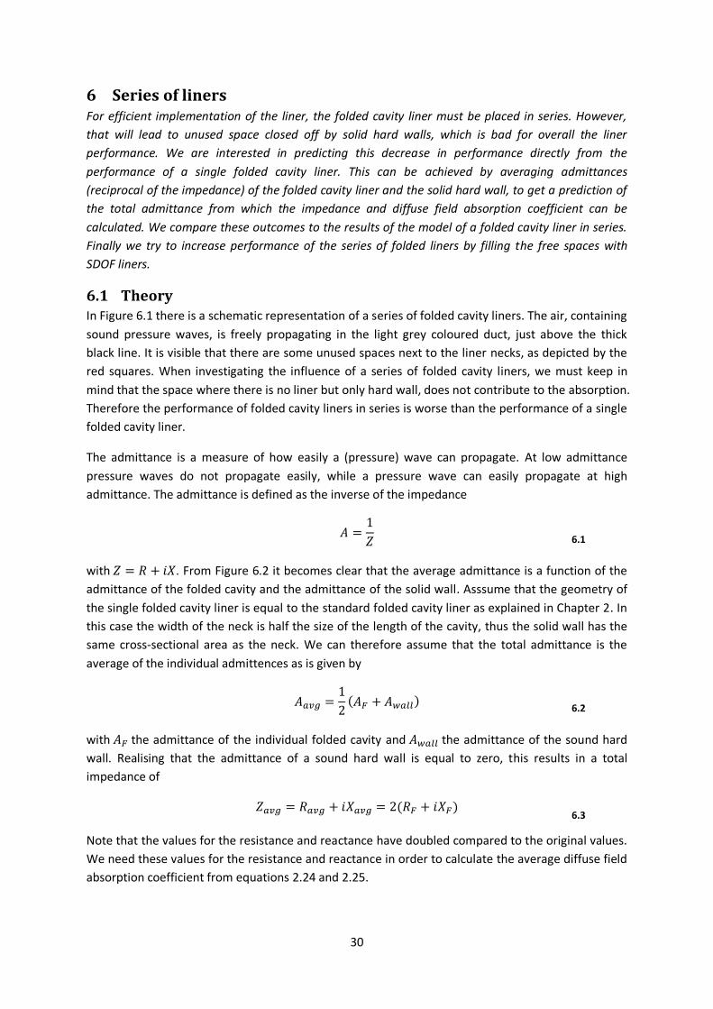
6.1 Theory In Figure 6.1 there is a schematic representation of a series of folded cavity liners. The air, containing
sound pressure waves, is freely propagating in the light grey coloured duct, just above the thick
black line. It is visible that there are some unused spaces next to the liner necks, as depicted by the
red squares. When investigating the influence of a series of folded cavity liners, we must keep in
mind that the space where there is no liner but only hard wall, does not contribute to the absorption.
Therefore the performance of folded cavity liners in series is worse than the performance of a single
folded cavity liner.
The admittance is a measure of how easily a (pressure) wave can propagate. At low admittance
pressure waves do not propagate easily, while a pressure wave can easily propagate at high
admittance. The admittance is defined as the inverse of the impedance
6.1
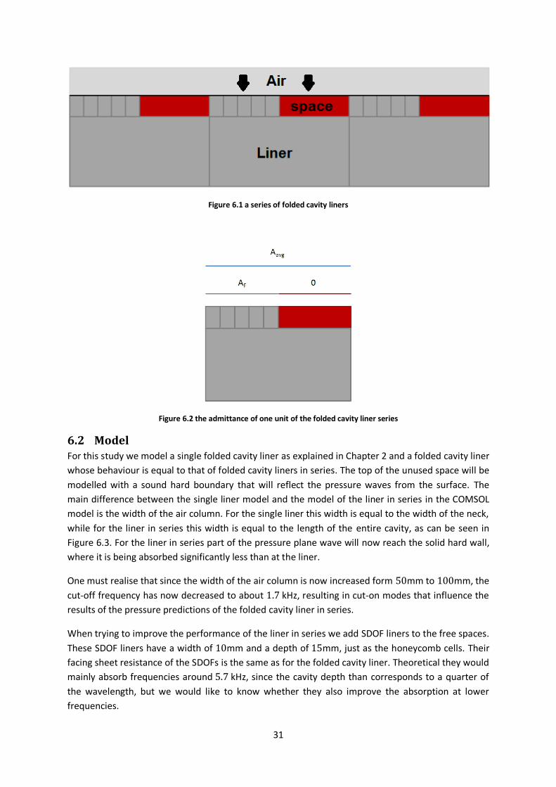
with . From Figure 6.2 it becomes clear that the average admittance is a function of the
admittance of the folded cavity and the admittance of the solid wall. Asssume that the geometry of
the single folded cavity liner is equal to the standard folded cavity liner as explained in Chapter 2. In
this case the width of the neck is half the size of the length of the cavity, thus the solid wall has the
same cross-sectional area as the neck. We can therefore assume that the total admittance is the
average of the individual admittences as is given by
6.2
with the admittance of the individual folded cavity and the admittance of the sound hard
wall. Realising that the admittance of a sound hard wall is equal to zero, this results in a total
impedance of
6.3
Note that the values for the resistance and reactance have doubled compared to the original values.
We need these values for the resistance and reactance in order to calculate the average diffuse field
absorption coefficient from equations 2.24 and 2.25.
31
Figure 6.1 a series of folded cavity liners
Figure 6.2 the admittance of one unit of the folded cavity liner series
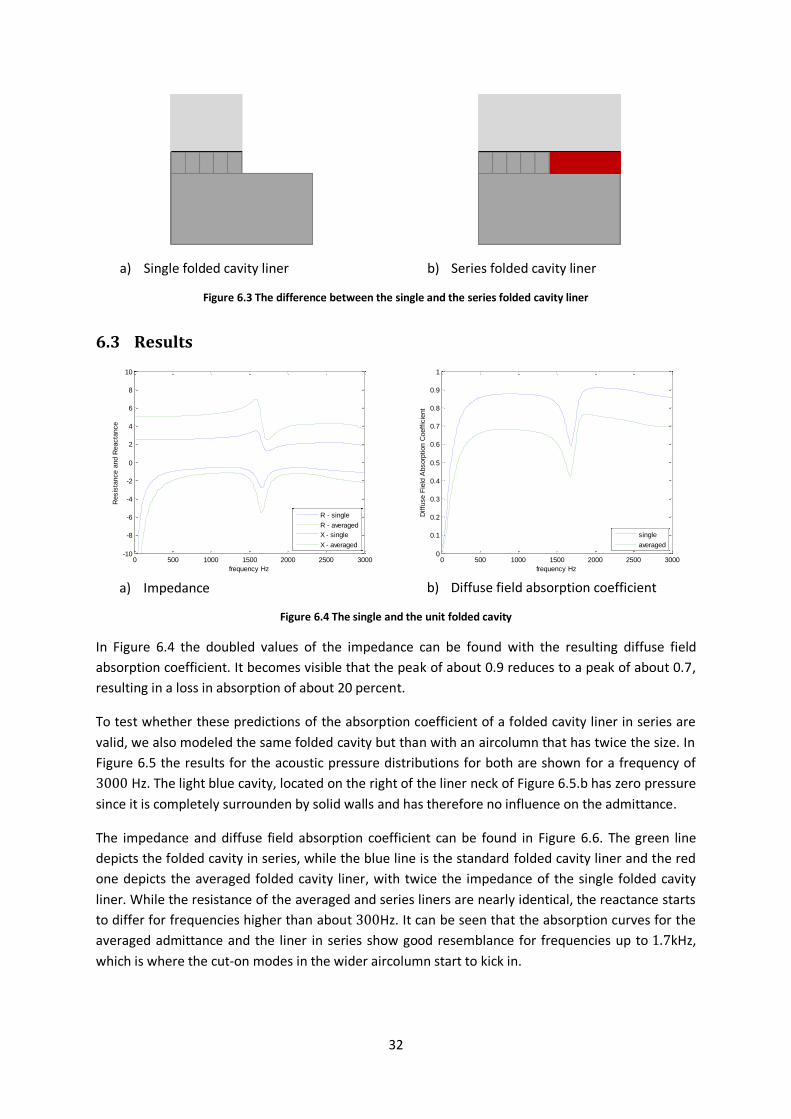
6.2 Model For this study we model a single folded cavity liner as explained in Chapter 2 and a folded cavity liner
whose behaviour is equal to that of folded cavity liners in series. The top of the unused space will be
modelled with a sound hard boundary that will reflect the pressure waves from the surface. The
main difference between the single liner model and the model of the liner in series in the COMSOL
model is the width of the air column. For the single liner this width is equal to the width of the neck,
while for the liner in series this width is equal to the length of the entire cavity, as can be seen in
Figure 6.3. For the liner in series part of the pressure plane wave will now reach the solid hard wall,
where it is being absorbed significantly less than at the liner.
One must realise that since the width of the air column is now increased form mm to mm, the
cut-off frequency has now decreased to about kHz, resulting in cut-on modes that influence the
results of the pressure predictions of the folded cavity liner in series.
When trying to improve the performance of the liner in series we add SDOF liners to the free spaces.
These SDOF liners have a width of mm and a depth of mm, just as the honeycomb cells. Their
facing sheet resistance of the SDOFs is the same as for the folded cavity liner. Theoretical they would
mainly absorb frequencies around kHz, since the cavity depth than corresponds to a quarter of
the wavelength, but we would like to know whether they also improve the absorption at lower
frequencies.
32
a) Single folded cavity liner b) Series folded cavity liner
Figure 6.3 The difference between the single and the series folded cavity liner
6.3 Results
a) Impedance b) Diffuse field absorption coefficient
Figure 6.4 The single and the unit folded cavity
In Figure 6.4 the doubled values of the impedance can be found with the resulting diffuse field
absorption coefficient. It becomes visible that the peak of about 0.9 reduces to a peak of about 0.7,
resulting in a loss in absorption of about 20 percent.
To test whether these predictions of the absorption coefficient of a folded cavity liner in series are
valid, we also modeled the same folded cavity but than with an aircolumn that has twice the size. In
Figure 6.5 the results for the acoustic pressure distributions for both are shown for a frequency of
Hz. The light blue cavity, located on the right of the liner neck of Figure 6.5.b has zero pressure
since it is completely surrounden by solid walls and has therefore no influence on the admittance.
The impedance and diffuse field absorption coefficient can be found in Figure 6.6. The green line
depicts the folded cavity in series, while the blue line is the standard folded cavity liner and the red
one depicts the averaged folded cavity liner, with twice the impedance of the single folded cavity
liner. While the resistance of the averaged and series liners are nearly identical, the reactance starts
to differ for frequencies higher than about Hz. It can be seen that the absorption curves for the
averaged admittance and the liner in series show good resemblance for frequencies up to kHz,
which is where the cut-on modes in the wider aircolumn start to kick in.
0 500 1000 1500 2000 2500 3000-10
-8
-6
-4
-2
0
2
4
6
8
10
frequency Hz
Resis
tance a
nd R
eacta
nce
R - single
R - averaged
X - single
X - averaged
0 500 1000 1500 2000 2500 30000
0.1
0.2
0.3
0.4
0.5
0.6
0.7
0.8
0.9
1
frequency Hz
Diffu
se F
ield
Absorp
tion C
oeff
icie
nt
single
averaged
33
a) Single folded cavity b) Folded cavity unit for a series of liners
Figure 6.5 difference between the single folded cavity model and the model of a model for a series of liners
a) Impedance b) Diffuse field absorption coefficient
Figure 6.6 comparison between theory and model
As remarked earlier the free space next to the liner necks is unused. We would like to know whether
filling them up with shallow SDOF liners is a usefull improvement on the absorption curves.
Therefore we modelled them with the same honeycomb width and length as of the folded cavity
liner neck. The acoustic pressure distributions for both the SDOF liner in series and the combination
of the folded cavity liner with the SDOF liners are shown in Figure 6.7.
The maximum in absorption for a SDOF liner with a depth of mm is expected to lie around kHz,
which is a lot higher than the frequency where the first cut-on modes appear. Therefore the
influence on the absorption curves is not expected to be significant for frequencies up to kHz.
However, any improvement on the absorption coefficient will be appreciated, since the space is not
being used in any other way. When looking at Figure 6.8 we can see that the placings of extra SDOF
liners does not increase the absorption performance of the folded cavity liner, but surprisingly even
decreases it. Therefore it is better not to fill the space up with extra liners, which would also cost
more money, but to leave it there.
0 500 1000 1500 2000 2500 3000-10
-8
-6
-4
-2
0
2
4
6
8
10
frequency Hz
Resis
tance a
nd R
eacta
nce
R - single
R - series
R - averaged
X - single
X - series
X - averaged
0 500 1000 1500 2000 2500 30000
0.1
0.2
0.3
0.4
0.5
0.6
0.7
0.8
0.9
1
frequency Hz
Diffu
se F
ield
Absorp
tion C
oeff
icie
nt
single
series
averaged
34
a) 5 SDOF liners, depth of 15 mm b) Combination of liners
Figure 6.7 acoustic pressure distributions of a) SDOF and b) the combined liner
a) Impedance b) Diffuse field absorption coefficient
Figure 6.8 comparison between the folded cavity with and without the SDOF liners
6.4 Conclusion It is shown that averaging the admittance of single folded cavity liner results in good prediction of
the behaviour of liners in series. However, it is also shown that filling up the free spaces between the
liner necks with SDOF liners decreases overall liner performance and is therefore not recommended.
0 500 1000 1500 2000 2500 3000-10
-8
-6
-4
-2
0
2
4
6
8
10
frequency Hz
Resis
tance a
nd R
eacta
nce
R - SDOF
R - Folded
R - Combined
X - SDOF
X - Folded
X - Combined
0 500 1000 1500 2000 2500 30000
0.1
0.2
0.3
0.4
0.5
0.6
0.7
0.8
0.9
1
frequency Hz
Diffu
se F
ield
Absorp
tion C
oeff
icie
nt
SDOF
Folded
Combined
35
7 Conclusion
It was shown that the 2D COMSOL liner model can predict the pressure, impedance and absorption
coefficients just as accurate as a 3D COMSOL. A comparison of the results with test data from the
NLR and Actran TM predictions led to the conclusion that the COMSOL model provides good
predictions up to the cut-of frequency of the duct.
When looking at the geometry of the folded cavity liner, it was shown that the length of the cavity
has the biggest influence on the location of the maximum of the absorption coefficient and the
resonance frequency, while the height of the column has a strong influence on the slope and the
width of the first absorption peak. On the contrast the width of the column appeared to have no
visible influence on frequencies up to Hz.
When looking at the resistive sheets, it is observed that the change in resistance of the facing sheet
results in the same change in the total acoustic resistance, but does not influence the reactance. It
must be noted that a high resistance facing sheet reduces the peak in the absorption with a
significant amount and is therefore not recommended. It was found that variations in the resistance
of the septum result in change in both the total resistance and reactance. Higher septum resistance
leads to a damping of the oscillations of the impedance. Placing a second septum can significantly
decrease deep troughs at unwanted locations and though it also affects the maximum absorption at
some points, those losses are only slight compared to the profit that can be made on other points.
Averaging the admittance of single folded cavity liner results in a good prediction of the behaviour of
folded cavity liners in series. However, it is also shown that filling up the free spaces between the
liner necks with SDOF liners is no improvement on the overall liner performance.
In this study the folded cavity liner was always modelled at the end of a duct, with a plane wave
propagating towards the inlet. The next step in understanding and predicting the behaviour of a
folded cavity liner in a intake duct would be to make a more accurate model of the intake duct.
Processes such as scattering of sound waves should be taken into account in order to effectively
predict the noise energy contributions of the pressure waves at each angle of incidence to the total
incoming pressure. This is needed to calculate the actual impedance and absorption as is
experienced in a lined engine intake.
36
Bibliography
[1] R. Motsinger and R. Kraft, “Design and performance of duct acoustic treatment,” in
Aeroacoustics of Flight Vehicles: Theory and Practice, vol. 2: Noise control (ed. H.H. Hubbard),
Hampton, Virginia, The Acoustical Society of America, 1995, pp. 165-206.
[2] R. J. Astley, “Propulsion System Noise: Turbomachinery,” in Encyclopedia of Aerospace
Engineering, John Wiley & Sons, 2010.
[3] R. Sugimoto, P. Murray and R. J. Astley, “Folded cavity liners for turbofan engine intakes,” in
AIAA/CEAS Aeroacoustics Conference, Colorado Springs, 2012.
[4] R. Sugimoto, R. J. Astley and P. Murray, “Computational analysis of folded cavity liners for
turbofan intakes,” in Internoise 2011, Osaka, 2011.
[5] R. J. Astley, “Numerical methods for noise propagation in moving flows, with application to
2. Go to the Settings window for Incident Pressure Field.
3. Locate the Boundary Selection section. From the Selection list, select Inlet.
4. Locate the Incident Pressure Field section. In the p0 edit field, type p0.
Interior Impedance 1
1. In the Model Builder window, right-click Model 1 > Pressure Acoustics and choose Interior
Impedance.
2. Go to the Settings window for Interior Impedance.
3. Locate the Boundary Selection section. From the Selection list, select Facingsheet.
4. Locate the Interior Impedance section. In the edit field, type
Interior Impedance 2
1. In the Model Builder window, right-click Model 1 > Pressure Acoustics and choose Interior
Impedance.
2. Go to the Settings window for Interior Impedance.
3. Locate the Boundary Selection section. From the Selection list, select Septum.
4. Locate the Interior Impedance section. In the edit field, type
Interior Sound Hard Boundary (Wall) 1
1. In the Model Builder window, right-click Model 1 > Pressure Acoustics and choose Interior
Sound Hard Boundary (Wall).
2. Go to the Settings window for Interior Sound Hard Boundary (Wall).
3. Locate the Boundary Selection section. From the Selection list, select Honeycomb cells.
X
MESH 1
Free Quad 1
1. In the Model Builder window, right-click Model 1 > Mesh 1 and choose Free Quad.
Size
1. In the Model Builder window, click Size.
2. Go to the Settings window for Size.
3. Locate the Element Size Parameters section. Click Custom.
4. In the Maximum element size edit field, type 10.
5. In the Minimum element size edit field, type 0.0375.
6. In the Maximum element growth edit field, type 1.2.
7. In the Resolution of curvature edit field, type 0.25.
8. In the Resolution of narrow regions edit field, type 1.
9. Click the Build All button.
STUDY 1
Step 1: Frequency Domain
1. In the Model Builder window, expand the Study 1 node, then click Step 1: Frequency
Domain.
2. Go to the Settings window for Frequency Domain.
3. Locate the Study Settings section. In the Frequencies edit field, type range(20,10,3500). This
setting will give you solutions from 20 to 3500 Hz, with a pitch of 10 Hz.
4. In the Model Builder window, right-click Study 1 and choose Compute.
RESULTS
Acoustic Pressure (acpr) The first one of the default plot shows the pressure distribution of the folded cavity liner at the highest frequency, 3500 Hz. To get a better view of the standing wave pattern, you can plot the norm of the pressure instead.
1. In the Model Builder window, expand the Acoustic Pressure (acpr) node, then click Surface
1.
2. Go to the Settings window for Surface.
3. In the upper-right corner of the Expression section, click Replace Expression.
4. From the menu, choose Pressure Acoustics>Absolute pressure (acpr.absp).
5. Click the Plot button.
The pattern is different for different frequencies. To change the frequency:
6. In the Model Builder window, click Acoustic Pressure (acpr).
7. Go to the Settings window for 2D Plot Group.
8. Locate the Data section. From the Parameter value (freq) list, select for instance 3000.
9. Click the Plot button.
XI
Cut Point 2D 1 1. In the Model Builder window, right-click on Results > Data Sets and choose Cut Point 2D
2. Go to the Settings window for Cut Point 2D.
3. Locate Point Data and expand. In the x edit field, type 25. In the y edit field, type 265.
4. Click the Plot button. There should now be a red dot in the middle of the top of the air
column.
1D Plot Group 3 - Impedance
1. In the Model Builder window, right-click Results and choose 1D Plot Group.
2. Right-click Results>1D Plot Group 3 and choose Point Graph.
3. Go to the Settings window for Point Graph.
4. Locate the Data section. In the Data Set edit field select Cut Point 2D 1.
5. Locate the y-Axis Data section. In the Expression edit field, type R.
6. Click to expand the Legends section.
7. Select the Show legends check box.
8. In the Legends edit field, select Manual.
9. Right-click Results>1D Plot Group 3 and choose Point Graph.
10. Go to the Settings window for Point Graph.
11. Locate the Data section. In the Data Set edit field select Cut Point 2D 1.
12. Locate the y-Axis Data section. In the Expression edit field, type X.
13. Click to expand the Legends section.
14. Select the Show legends check box.
15. In the Legends edit field, select Manual.
16. In the Model Builder window, click Results > 1D Plot Group.
17. In the Settings window expand the Axis section.
18. Select the Manual axis limits box. In the y minimum field, type -10 and in the y maximum
field, type 10
19. Click the Plot button. The graph should now look like Fig 2.
1D Plot Group 4 – Diffuse field absorption coefficient
1. In the Model Builder window, right-click Results and choose 1D Plot Group.
2. Right-click Results>1D Plot Group 4 and choose Point Graph.
3. Go to the Settings window for Point Graph.
4. Locate the Data section. In the Data Set edit field select Cut Point 2D 1.
5. Locate the y-Axis Data section. In the Expression edit field, type a.
6. In the Model Builder window, click Results > 1D Plot Group.
7. In the Settings window expand the Axis section.
8. Select the Manual axis limits box. In the y minimum field, type 0 and in the y maximum field,
type 1.
9. Click the Plot button. The graph should now look like Fig 3.
XII
EXPORT
Data 1 - R
1. In the Model Builder window, right-click Results > Data Sets > Cut Point 2D 1 and choose
Add data to Export.
2. Go to the Settings window for Export.
3. In the Expression field, type R.
4. Make sure all frequencies you want to export are selected.
5. Click to expand the Advanced section.
6. De-select the Include header and the Full precision boxes.
7. In the Output section enter the filename with the location on the computer where you want
the text file with your results to appear. (for instance C:\R.txt)
Data 2 - X
1. In the Model Builder window, right-click Results > Data Sets > Cut Point 2D 1 and choose
Add data to Export.
2. Go to the Settings window for Export.
3. In the Expression field, type X.
4. Make sure all frequencies you want to export are selected.
5. Click to expand the Advanced section.
6. De-select the Include header and the Full precision boxes.
7. In the Output section enter the filename with the location on the computer where you want
the text file with your results to appear. (for instance C:\X.txt)
Data 3 - a
1. In the Model Builder window, right-click Results > Data Sets > Cut Point 2D 1 and choose
Add data to Export.
2. Go to the Settings window for Export.
3. In the Expression field, type a.
4. Make sure all frequencies you want to export are selected.
5. Click to expand the Advanced section.
6. De-select the Include header and the Full precision boxes.
7. In the Output section enter the filename with the location on the computer where you want
the text file with your results to appear. (for instance C:\a.txt)
8. Right-click Results > Export to export data.
These text files can now be imported by Matlab for easy post processing. Note that the first two
numbers of the exported file are the x and the y coordinates of the chosen data point.