Internship Report - Universiteit Twenteessay.utwente.nl/69528/1/Internship Report Final_.pdf ·...

Internship Report

Assessment of influence of play in joints on the end

effector accuracy in a novel 3DOF (1T-2R) parallel

manipulator

Vinayak J. Kalas

(MSc – Mechanical Engineering, University of Twente)

Advisors:

ir. A.G.L. Hoevenaars (Delft Haptics Lab, Delft University of Technology)

prof. dr. ir J.L. Herder (University of Twente)

Acknowledgement

I would like to express my sincere gratitude to my supervisor from TU Delft, Teun

Hoevenaars, for his constant guidance that kept me on track with the defined

objectives and helped me in having clarity of thought at different stages of my

research.

I would like to extend my appreciation to prof. Just Herder for his guidance and

support.

Finally, I would like to thank all the researchers at the Delft Haptics lab for

interesting discussions and valuable inputs at various stages of the research.

Preface

This internship assignment was carried out at TU Delft and was a compulsory

module as a part of my Master studies in Mechanical Engineering at the

University of Twente. This internship was carried out for a period of 14 weeks,

from 16th of November 2015 to 19th of February 2016, and during this period I

was exposed to different research projects being carried out at the Delft Haptics

lab, apart from in-depth knowledge of the project I was working on.

The main objectives of this internship assignment were to get acquainted with

Parallel Kinematics, which included deep understanding of Screw theory and its

application to parallel manipulator analysis, and to get acquainted with various

methods to assess the effects of play at the joints of parallel mechanisms on the

end effector accuracy.

To achieve the same, the influence of play on the static performance (end

effector accuracy) of a novel 3-DOF (1T-2R) parallel manipulator, which is

intended to act as a haptic master device for steerable needles, was tried to

analyze. The device being a limited-DOF parallel manipulator has some

constrained directions and the play at the ball bearings affects the performance

and quantifying this was the main aim of this internship.

Contents

1. Introduction 1

2. A Brief Summary of Screw Theory 2

3. Literature Survey 9

4. Method to model effect of play in joint on the end effector accuracy 11

5. Application of play modelling to the 3-DOF haptic master device 17

6. Results and discussion 22

References 23

Appendix 24

1

1. Introduction

Parallel manipulators have had an indelible impact on industry applications in

the past few years due to its inherent advantages in terms of accuracy as

compared to serial manipulators, although some [1] have pointed out that this

question of superiority is debatable. However, the consideration of accuracy is

always crucial in terms of demand that different applications have and there are

various factors that can hamper this. One of the main factors affecting the end

effector accuracy are the clearances in joints. The effect of clearance on the

positioning error and accuracy of parallel manipulators has been looked into by

many authors over decades and brief overview of different approaches is

summarized here. The problem of modelling joint clearance in mechanisms and

assessing its effect on the pose (position and orientation) error has been

approached by different methods, however, most of them were limited to planar

or single loop mechanisms and their extension to analysis of effects in parallel

manipulators was not addressed (in some cases) or was not demonstrated.

The current study aims at analyzing the effects of clearance on a novel 3-DOF

parallel manipulator intended to act as a haptic master device. The

aforementioned device has universal and revolute joints and the play in the

constrained directions are mainly due to clearance in the revolute joints. This

report discusses screw theory in brief and then goes on to provide a brief

literature survey of various relevant methods of modelling the play at joints and

then describes the implementation of the selected method of modelling on the

system under study. During the implementation of the selected method, certain

problems were encountered which are discussed later in this report and given

the timeframe of this assignment, a detailed analysis of the same was not

possible and possible explanations are summarized at the end.

2

2. A Brief Summary of Screw Theory

Screw theory is one of the strongest tools for analysis of robotic manipulators

and it uses a combination of algebra and calculus of pair of vectors such as forces,

moments, angular and linear velocities to do so. This section provides a brief

introduction to Screw theory and a comprehensive overview of important

concepts used in parallel kinematics is given. [2] is used as a reference for all the

figures and references for detailed information.

2.1. Description of screw motion

Screw motion is described as rigid body motion consisting of a rotation

about an axis through an angle, followed by translation along the same

axis. Figure 2.1 shows the description of a general screw motion.

Figure 2.1: General screw [2]

Since this motion resembles the motion of a screw, it is called screw

motion. Further, the pitch of a screw motion is defined to be the ratio

of translation to rotation, h = d/θ, where d is the translation and θ is

the rotation about the axis in radians.

Thus the net translational motion after θ radians of rotation about the

axis is hθ. The axis is then represented as a directed line through a

point; choosing q ϵ R3 as the point on the axis and ω ϵ R3 as the unit

vector specifying the direction. The axis is then a set of points defined

by

l = (q + λω: λ ϵ R) (2.1)

3

The above definitions are valid when the screw motion consists of a

nonzero rotation followed by translation. In case of zero rotation, we

consider the axis as a line through the origin in the direction v and the

magnitude of this vector is 1. The pitch of this screw is ∞ and the

amount of translation along the direction v is given by its magnitude.

2.2. Twists and Wrenches

Now that we know the description of screw, we can go ahead to

describe velocities and forces using this description of screw. Twists

are generalization of velocities of rigid bodies and any rigid body

motion can be expressed using a twist. Geometrically, these are

elements of the Lie algebra se(3) associated to the Lie group SE(3). For

a more mathematical understanding of the theory of twists, the reader

is referred to section 3.2 to section 3.3 of chapter 1 of [2]. To

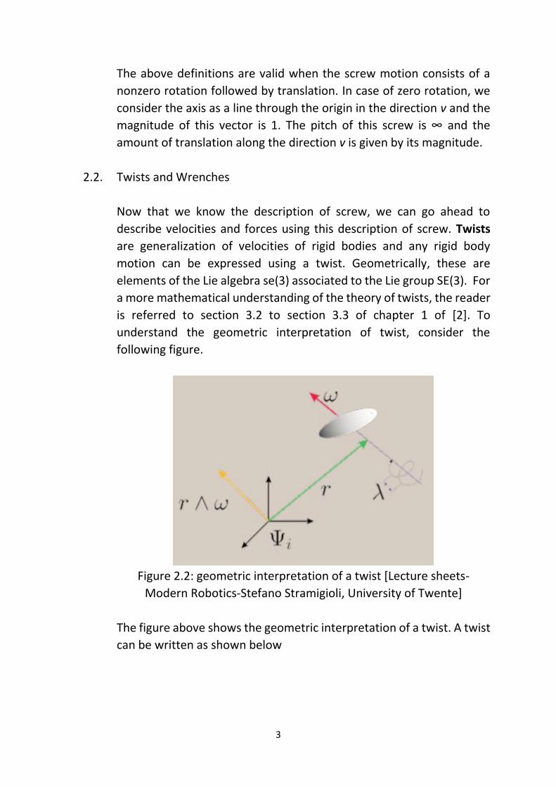
understand the geometric interpretation of twist, consider the

following figure.

Figure 2.2: geometric interpretation of a twist [Lecture sheets-

Modern Robotics-Stefano Stramigioli, University of Twente]

The figure above shows the geometric interpretation of a twist. A twist

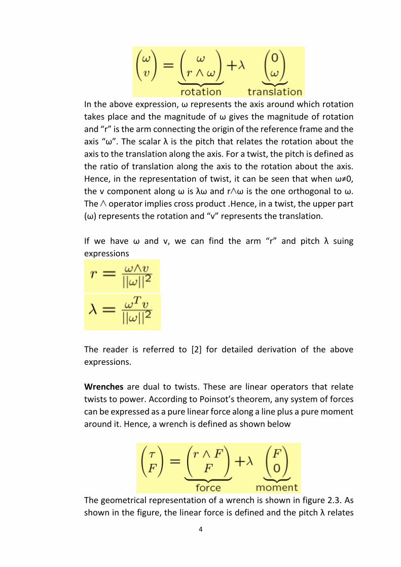
can be written as shown below

4

In the above expression, ω represents the axis around which rotation

takes place and the magnitude of ω gives the magnitude of rotation

and “r” is the arm connecting the origin of the reference frame and the

axis “ω”. The scalar λ is the pitch that relates the rotation about the

axis to the translation along the axis. For a twist, the pitch is defined as

the ratio of translation along the axis to the rotation about the axis.

Hence, in the representation of twist, it can be seen that when ω≠0,

the v component along ω is λω and r ω is the one orthogonal to ω.

The operator implies cross product .Hence, in a twist, the upper part

(ω) represents the rotation and “v” represents the translation.

If we have ω and v, we can find the arm “r” and pitch λ suing

expressions

The reader is referred to [2] for detailed derivation of the above

expressions.

Wrenches are dual to twists. These are linear operators that relate

twists to power. According to Poinsot’s theorem, any system of forces

can be expressed as a pure linear force along a line plus a pure moment

around it. Hence, a wrench is defined as shown below

The geometrical representation of a wrench is shown in figure 2.3. As

shown in the figure, the linear force is defined and the pitch λ relates

5

the linear force F to the moment about the axis. The pitch in a wrench

is defined as the ratio of angular rotation about the axis to the linear

force. The reader is referred to section 5 of chapter 1 in [2] for more

detailed mathematical explanation of wrenches.

Figure 2.3: geometric interpretation of a wrench [Lecture sheets-

Modern Robotics-Stefano Stramigioli, University of Twente]

2.3. Reciprocity and Applications

The dot product of wrenches and twist gives the instantaneous power

associated with the moving rigid body under the influence of applied

force. A wrench F is then said to be reciprocal to a twist V if the

instantaneous power is zero, i.e., F . V = 0. Let V be the twist about

screw S1 and let F be the wrench along the screw S2. The reciprocal

product between a twist and a wrench, expressed in screw

coordinates, is then defined as follows.

For a twist

6

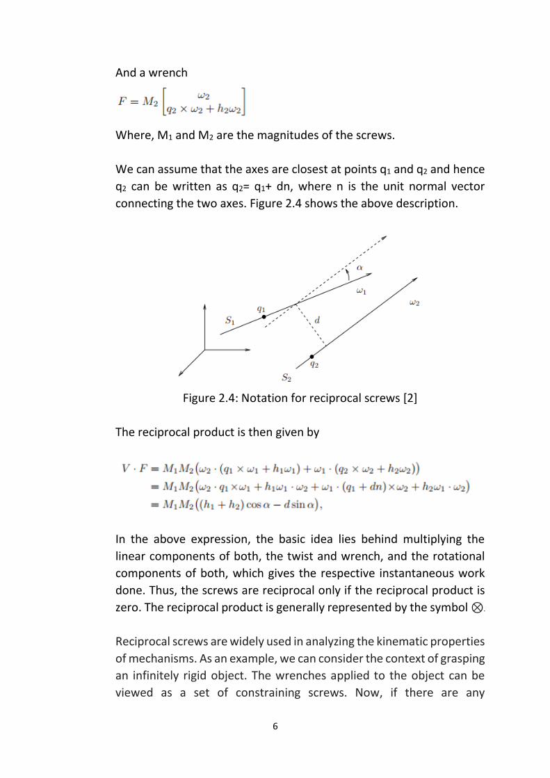
And a wrench

Where, M1 and M2 are the magnitudes of the screws.

We can assume that the axes are closest at points q1 and q2 and hence

q2 can be written as q2= q1+ dn, where n is the unit normal vector

connecting the two axes. Figure 2.4 shows the above description.

Figure 2.4: Notation for reciprocal screws [2]

The reciprocal product is then given by

In the above expression, the basic idea lies behind multiplying the

linear components of both, the twist and wrench, and the rotational

components of both, which gives the respective instantaneous work

done. Thus, the screws are reciprocal only if the reciprocal product is

zero. The reciprocal product is generally represented by the symbol ⊗.

Reciprocal screws are widely used in analyzing the kinematic properties

of mechanisms. As an example, we can consider the context of grasping

an infinitely rigid object. The wrenches applied to the object can be

viewed as a set of constraining screws. Now, if there are any

7

instantaneous motions (twists), then these correspond to motions that

are not constrained by the applied wrench and hence the reciprocal

product of these twists with the applied wrenches are then 0, implying

that the applied wrenches have no contribution to

generating/restricting these twists. A noteworthy example to mention

here would be [3] in which the authors have shown that the Jacobian

of a limited DOF parallel manipulator can be derived making use of the

theory of reciprocal screws.

2.4. Coordinate transformation

Now that we know about how velocities and forces can be represented

using screw coordinates, it’s handy to know how the coordinate

transformation can be performed for them. This is a very useful tool

for kinematic analysis of mechanisms. The reader is referred to section

4.4 of chapter 2 of [2] for more detailed information.

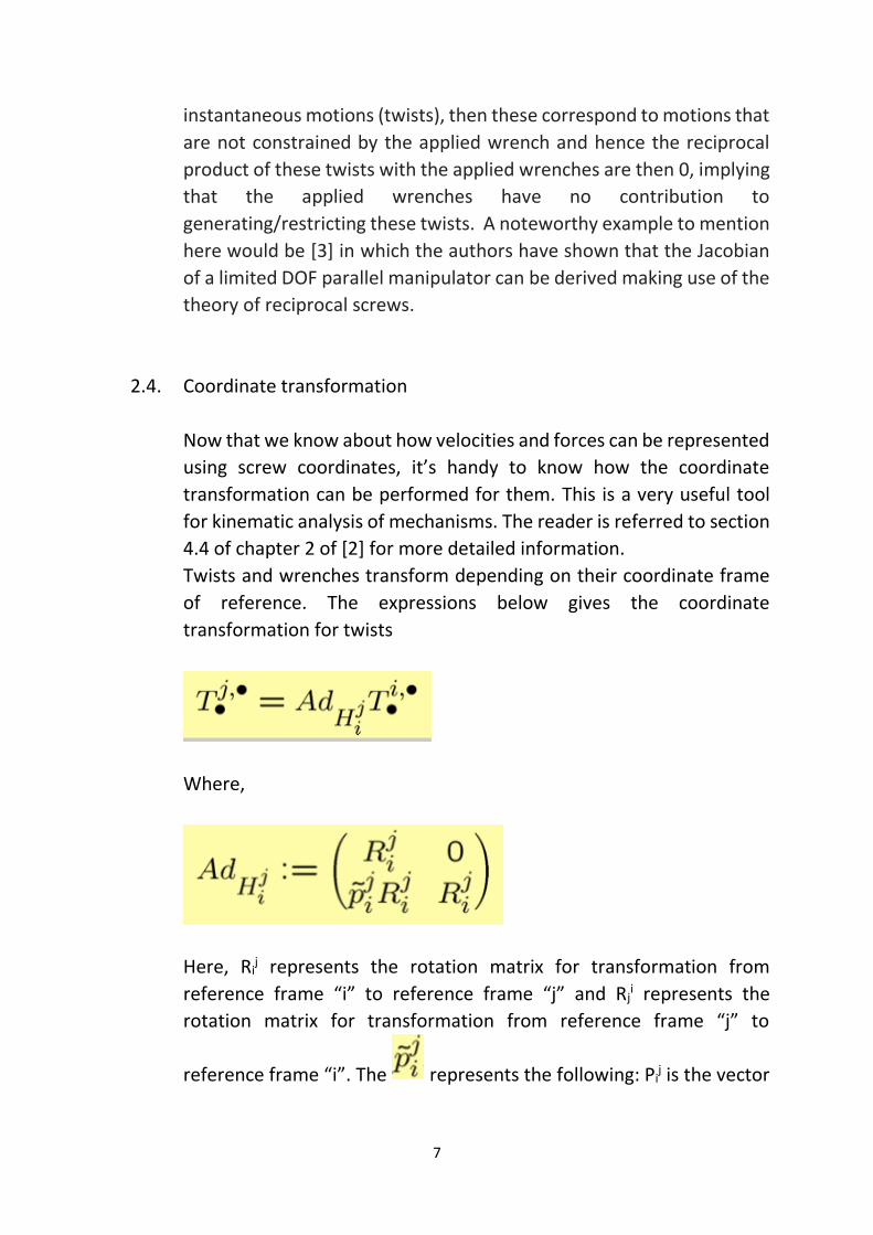
Twists and wrenches transform depending on their coordinate frame

of reference. The expressions below gives the coordinate

transformation for twists

Where,

Here, Rij represents the rotation matrix for transformation from

reference frame “i” to reference frame “j” and Rji represents the

rotation matrix for transformation from reference frame “j” to

reference frame “i”. The represents the following: Pij is the vector

8

connecting the origin of reference frame “i” to that of reference frame

“j”.

For, Pij = [p1 p2 p3]T

is given by,

0 -p3 p2

p3 0 -p1

-p2 p1 0

Similarly, the coordinate transformation of wrenches is given by the

following expression

Where

9

3. Literature Survey

In this section, a summary of the literature survey performed to find the different

modelling techniques to model the effect of play in joints on end effector

performance is summarized. Some authors concentrated on the dynamic effects

of clearance (Flores, Ambrósio [4]), such as impacts in pairs and vibrations,

whereas some concentrated on kinematic modelling Parenti-Castelli and

Venanzi [5], Venanzi and Parenti-Castelli [6], which is more helpful for

preliminary analysis of mechanism performance. Most approaches of analyzing

the effects of clearances can be broadly classified into stochastic and

deterministic methods. Stochastic methods (Dhande and Chakraborty [7], Wei-

Liang and Qi-Xian [8], Chaker, Mlika [9]) describe the clearance due to

displacement through probability distribution function and Deterministic

methods (Venanzi and Parenti-Castelli [6], Innocenti [10], Parenti-Castelli and

Venanzi [5]) try to exactly determine the displacement of the mechanism links.

Wu and Rao [11] used the method of intervals to model clearance and

manufacturing errors.

A screw theory method was presented by Tsai and Lai [12] to analyze the

transmission performance of linkages that have joint clearance by treating the

joint clearances as virtual links in this study, but this method was valid only for

planar mechanisms and the effectiveness was demonstrated only for single loop

linkages. An extension of this method to multi loop linkages was presented in

Tsai and Lai [13], but again was valid only for planar mechanisms. The main

drawback of this method, i.e., it’s limitation to planar mechanism analysis, was

overcome in methods proposed by Parenti-Castelli and Venanzi [5]. They showed

a method to evaluate the clearance influence in spatial parallel mechanisms with

focus on kinematic modelling and by using the principle of virtual work. Venanzi

and Parenti-Castelli [6] used a deterministic technique to assess the effect of

clearance for both planar and spatial, open-, and closed-chain mechanisms (not

for over constrained mechanisms). The method uses a kinematic approach to do

so. In this method, the clearances are modeled as virtual generalized

displacement and local models are defined for different joint pairs and

maximization of pose error function is carried out to determine the largest

possible error. Chaker, Mlika [9] analyzed a spherical parallel manipulator with

clearance and manufacturing errors by modelling the clearance and

manufacturing errors as small displacements and by using screw theory and

stochastic results were presented. They proved that the method of

10

superposition doesn’t work when both manufacturing error and clearance are

considered. Frisoli, Solazzi [14] used a method based on screw theory to estimate

the pose accuracy in spatial parallel manipulators with revolute joint clearance.

This method performs a 2 step maximization ( the first step gives a suboptimal

estimation of the pose error function and the second step is an iterative

numerical procedure) pose error function and the pose error is a quadratic

function of the end-effector displacement, and can converge to exact maximum

pose error in a limited number of iterations. The effectiveness of this method

has been demonstrated with application examples where worst case angular and

linear position accuracy in translating fully parallel manipulators is determined.

Since this investigation is very close (in terms of study on clearance in revolute

joints) to the study performed by Frisoli, Solazzi [14], the method used by them

will be used for analyzing the clearance effect on end effector performance and

look into ways to redesign the haptic master device to reduce the play below

human thresholds.

11

4. Method to model the effect of play in joints on the end

effector accuracy

The following method was described in Frisoli, Solazzi [14]. This is a method

based on screw theory for the analysis of position accuracy in spatial parallel

manipulators with revolute joints clearances and since our system of interest

also has revolute joints (only), this is a very good reference study.

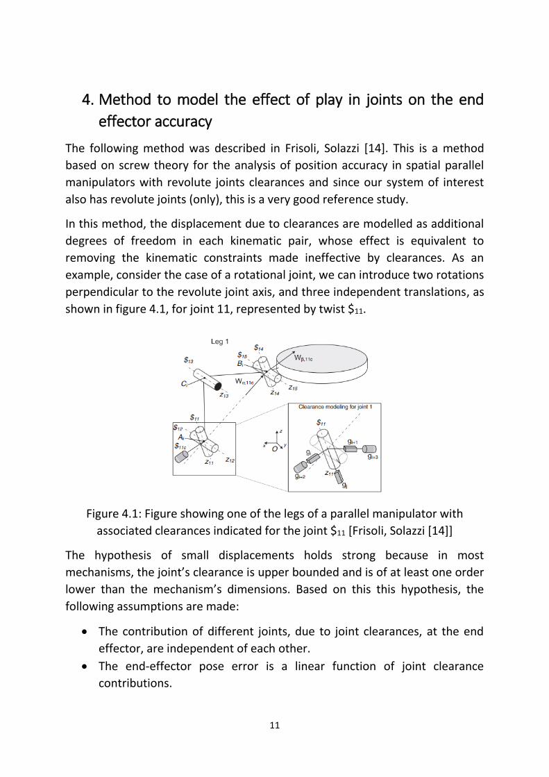
In this method, the displacement due to clearances are modelled as additional

degrees of freedom in each kinematic pair, whose effect is equivalent to

removing the kinematic constraints made ineffective by clearances. As an

example, consider the case of a rotational joint, we can introduce two rotations

perpendicular to the revolute joint axis, and three independent translations, as

shown in figure 4.1, for joint 11, represented by twist $11.

Figure 4.1: Figure showing one of the legs of a parallel manipulator with

associated clearances indicated for the joint $11 [Frisoli, Solazzi [14]]

The hypothesis of small displacements holds strong because in most

mechanisms, the joint’s clearance is upper bounded and is of at least one order

lower than the mechanism’s dimensions. Based on this this hypothesis, the

following assumptions are made:

The contribution of different joints, due to joint clearances, at the end

effector, are independent of each other.

The end-effector pose error is a linear function of joint clearance

contributions.

12

Velocity analysis can be used to study the effect of clearances and screw

theory can be used to represent the induced infinitesimal displacements.

The pose of the mechanism affects the influence of each clearance on the

overall displacement of the end effector.

4.1. Obtaining the associated twists

Consider a parallel manipulator, whose generic leg is represented in

figure 4.1. Assume all the active DOFs locked by the actuators

(represented as darkened) so that the mechanism is statically

determined and has a mobility of zero according to Grubler’s criterion.

Assume an isostatic distribution of reaction forces, which are a system of

six linearly independent constraint wrenches [Wim], with subscript

i=1,….,ni indicating the leg number and m=1,….,nm the wrench number.

They represent the active and passive constraints of the kinematic chains

of the mechanism, according to [3]. Figure 4.2 shows a 3URU (universal-

revolute-universal, indicating the types of joints in each leg) parallel

manipulator, with Wi1, i=1,2,3 are the actuation wrenches of zero pitch

and Wi2, i=1,2,3 are the passive constraint wrenches of infinite pitch for

leg i.

Figure 4.2: Kinematics of 3URU parallel manipulator. Manipulator

actuated at joints C1, C2 and C3. [14]

13

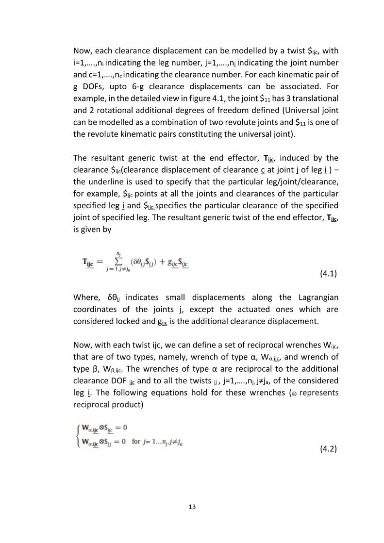
Now, each clearance displacement can be modelled by a twist $ijc, with

i=1,….,ni indicating the leg number, j=1,….,nj indicating the joint number

and c=1,….,nc indicating the clearance number. For each kinematic pair of

g DOFs, upto 6-g clearance displacements can be associated. For

example, in the detailed view in figure 4.1, the joint $11 has 3 translational

and 2 rotational additional degrees of freedom defined (Universal joint

can be modelled as a combination of two revolute joints and $11 is one of

the revolute kinematic pairs constituting the universal joint).

The resultant generic twist at the end effector, Tijc, induced by the

clearance $ijc(clearance displacement of clearance c at joint j of leg i ) –

the underline is used to specify that the particular leg/joint/clearance,

for example, $ijc points at all the joints and clearances of the particular

specified leg i and $ijc specifies the particular clearance of the specified

joint of specified leg. The resultant generic twist of the end effector, Tijc,

is given by

(4.1)

Where, δθij indicates small displacements along the Lagrangian

coordinates of the joints j, except the actuated ones which are

considered locked and gijc is the additional clearance displacement.

Now, with each twist ijc, we can define a set of reciprocal wrenches Wijc,

that are of two types, namely, wrench of type α, Wα,ijc, and wrench of

type β, Wβ,ijc. The wrenches of type α are reciprocal to the additional

clearance DOF ijc and to all the twists ij , j=1,….,nj, j≠ja, of the considered

leg i. The following equations hold for these wrenches (⊗ represents

reciprocal product)

(4.2)

14

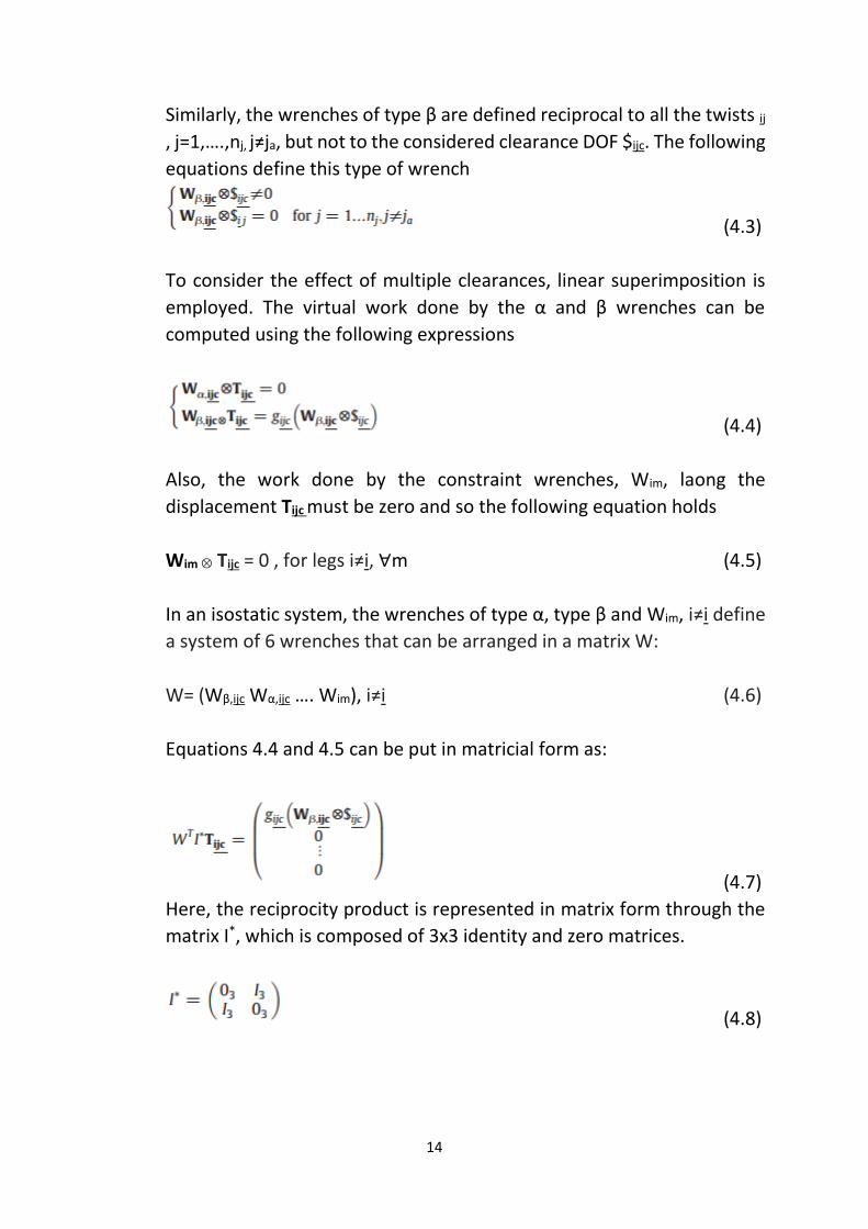
Similarly, the wrenches of type β are defined reciprocal to all the twists ij , j=1,….,nj, j≠ja, but not to the considered clearance DOF $ijc. The following

equations define this type of wrench

(4.3)

To consider the effect of multiple clearances, linear superimposition is

employed. The virtual work done by the α and β wrenches can be

computed using the following expressions

(4.4)

Also, the work done by the constraint wrenches, Wim, laong the

displacement Tijc must be zero and so the following equation holds

Wim ⊗ Tijc = 0 , for legs i≠i, ∀m (4.5)

In an isostatic system, the wrenches of type α, type β and Wim, i≠i define

a system of 6 wrenches that can be arranged in a matrix W:

W= (Wβ,ijc Wα,ijc …. Wim), i≠i (4.6)

Equations 4.4 and 4.5 can be put in matricial form as:

(4.7)

Here, the reciprocity product is represented in matrix form through the

matrix I*, which is composed of 3x3 identity and zero matrices.

(4.8)

15

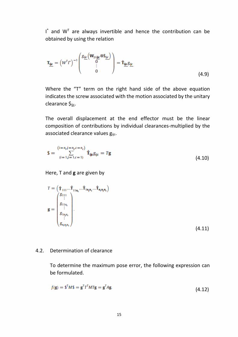
I* and WT are always invertible and hence the contribution can be

obtained by using the relation

(4.9)

Where the “T” term on the right hand side of the above equation

indicates the screw associated with the motion associated by the unitary

clearance $ijc.

The overall displacement at the end effector must be the linear

composition of contributions by individual clearances-multiplied by the

associated clearance values gijc.

(4.10)

Here, T and g are given by

(4.11)

4.2. Determination of clearance

To determine the maximum pose error, the following expression can

be formulated.

(4.12)

16

Where, M is a metrics matrix and is positive definite and symmetric and

f(g) is a cost function that has to be maximized to obtain the worst

possible error.

Since this analysis is limited to rotational joints, the clearances in the

joints are modelled as small displacements and based on this two types

of constraints are defined. These two types of constraints define the

maximization clearance problem to find a suboptimal estimate of the

maximum clearance. Taking this suboptimal solution as the starting

point, the optimal value of maximum clearance is obtained through

gradient descent maximization procedure. The reader can refer section

3 of [14] for detailed derivation and explanation in this regard.

4.3. Final effect quantified

Once the maximum clearance value matrix is obtained, the matrix of

individual twist contributions, T, and the matrix of maximum clearance

values, g, are substituted in equation 4.10 to obtain the final twist at of

the end effector.

17

5. Application of play modelling to the 3-DOF Haptic Master

device

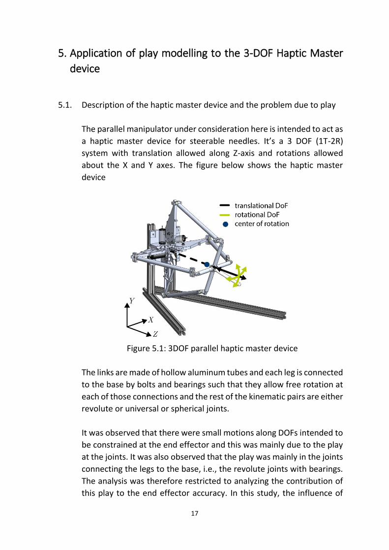
5.1. Description of the haptic master device and the problem due to play

The parallel manipulator under consideration here is intended to act as

a haptic master device for steerable needles. It’s a 3 DOF (1T-2R)

system with translation allowed along Z-axis and rotations allowed

about the X and Y axes. The figure below shows the haptic master

device

Figure 5.1: 3DOF parallel haptic master device

The links are made of hollow aluminum tubes and each leg is connected

to the base by bolts and bearings such that they allow free rotation at

each of those connections and the rest of the kinematic pairs are either

revolute or universal or spherical joints.

It was observed that there were small motions along DOFs intended to

be constrained at the end effector and this was mainly due to the play

at the joints. It was also observed that the play was mainly in the joints

connecting the legs to the base, i.e., the revolute joints with bearings.

The analysis was therefore restricted to analyzing the contribution of

this play to the end effector accuracy. In this study, the influence of

18

play in the joint connecting the right leg (as in figure 5.1) to the base is

studied.

The procedure as outlined in section 4 of this report was employed.

5.2. Defining twists

First, the twists representing the joints and virtual joints were defined.

The origin of frame of reference was assumed to be at the center of

the base. The fig below shows the right leg with its joint

representations.

Figure 5.2: Right leg of the haptic master device

Z21…..Z24 represent the versors aligned along the joints of the leg. The

unit twists representing these joints are denoted as $21….$24. The figure

below shows joint $21 along with the associated virtual degrees of

freedom, which is also our joint of interest.

19

Figure 5.3: Joint 1 and its associated virtual DOFs

The figure above shows the associated virtual degrees of freedom,

which are 2 rotational and 3 translational DOFs. Z21 is the versor along

the revolute joint considered and Z21z is the versor perpendicular to Z21

and oriented along Z-axis. The unit twist associated with joint 1 is given

by

$21 = (

𝑍21

(𝐴2 − 𝑂) × 𝑍21)

(5.1)

The unit twists representing the virtual DOFs are given by

$211 = (𝜔21

(𝐴2 − 𝑂) × 𝜔21) (5.2)

Where, ω211 = Z21 x Z21z / || Z21 x Z21z||

$212 = (0

𝜔212) (5.3)

Where, ω212 = Z21 x Z21z / || Z21 x Z21z||

$213 = (

𝑍21𝑧

(𝐴2 − 𝑂) × 𝑍21𝑧)

(5.4)

$214 = (0

𝑍21𝑧) (5.5)

20

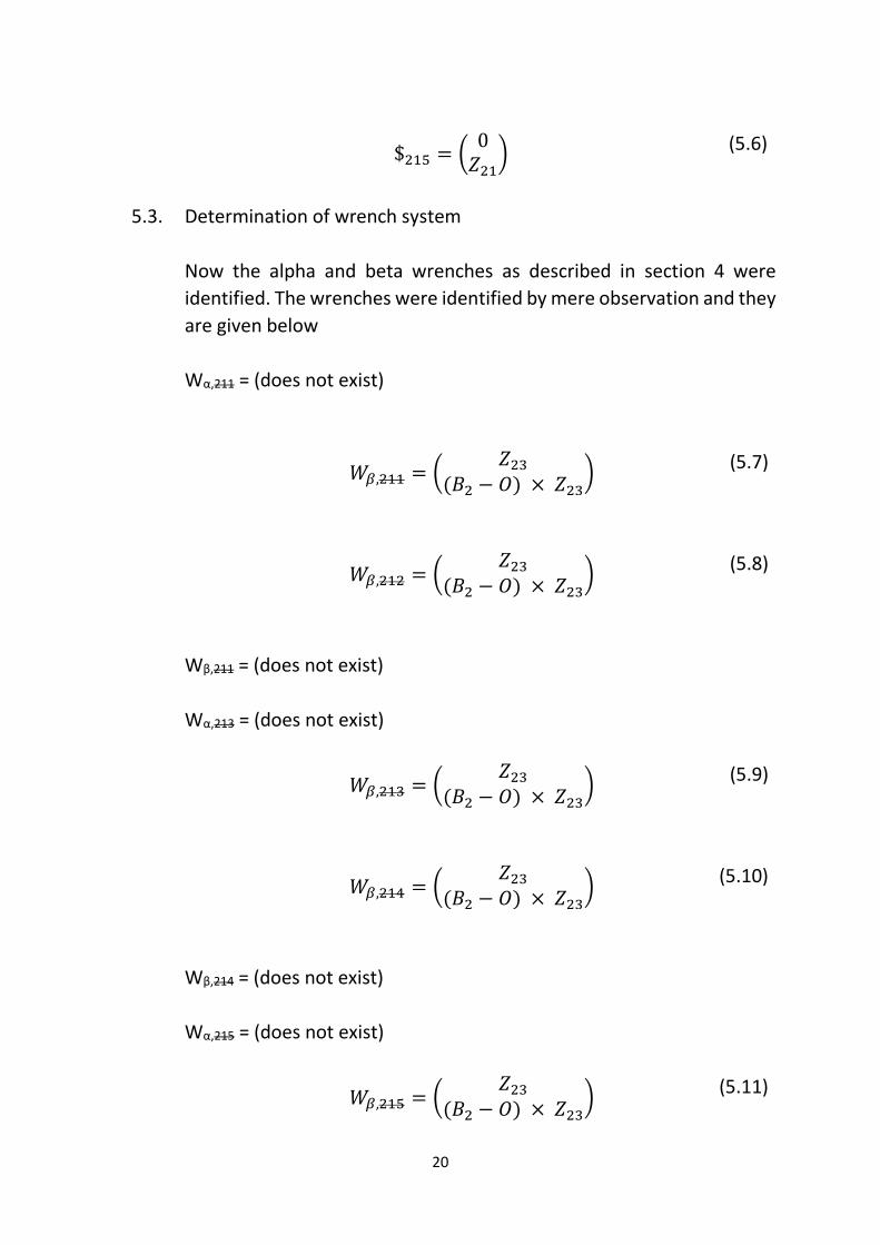
$215 = (0

𝑍21) (5.6)

5.3. Determination of wrench system

Now the alpha and beta wrenches as described in section 4 were

identified. The wrenches were identified by mere observation and they

are given below

Wα,211 = (does not exist)

𝑊𝛽,211 = (

𝑍23

(𝐵2 − 𝑂) × 𝑍23)

(5.7)

𝑊𝛽,212 = (

𝑍23

(𝐵2 − 𝑂) × 𝑍23)

(5.8)

Wβ,211 = (does not exist)


𝑊𝛽,213 = (

𝑍23

(𝐵2 − 𝑂) × 𝑍23)

(5.9)

𝑊𝛽,214 = (

𝑍23

(𝐵2 − 𝑂) × 𝑍23)

(5.10)

Wβ,214 = (does not exist)


𝑊𝛽,215 = (

𝑍23

(𝐵2 − 𝑂) × 𝑍23)

(5.11)

21

The constraint wrenches were defined for the other legs that

constitute the W matrix as in equation 4.10.

5.4. Solving the system of equations

Once the wrenches and twists are defined, the system of equations as

shown in section 4 are solved. Equation 4.9 is solved to obtain the

individual twists and then the maximum clearance matrix is obtained

using the procedure outlined in [14] and the final twist of the end

effector is calculated using equation 4.10. This was formulated in

MATLAB and the code is given in Appendix A1.

22

6. Results and discussion

Appendix A2 shows the result after running the code. The following

problems were encountered in the implementation of the procedure

outlined in [14]:

The “WT I*” matrix in equation 4.9 was a rank deficient matrix since

one of our constraint wrenches from other legs was zero and also

in some cases, the alpha and/or beta wrench was zero. Hence, the

inverse of the matrix didn’t exist. This led us to taking the

pseudoinverse of the matrix for further analysis.

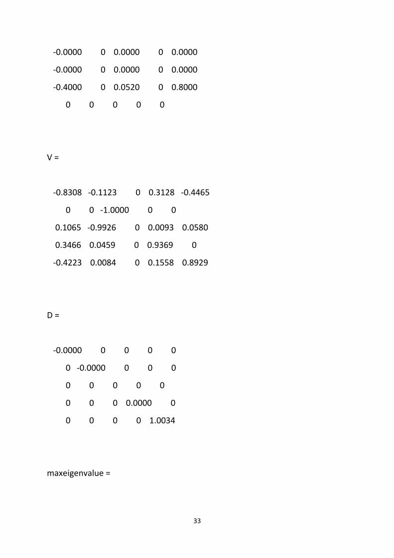
The obtained twist matrix “T” was found to be a rank deficient

matrix implying that the twist contributions from the individual

virtual DOFs were dependent/related (since they were same

vectors were different scaling).

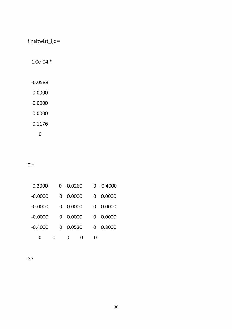
The implementation of the method to obtain maximum clearance

was unsuccessful as the results obtained were very unrealistic.

Although the physical interpretation of the obtained twists for the end

effector look acceptable(the directions of translation are expected) ,

the inability to obtain the exact numerical values for the exact

influence of the joint on the end effector pose error remains a major

setback of this research. Also, the reason for dependent twist matrix is

unknown and hence the results obtained (twists of the end effector)

can be doubted for their correctness.

This research had to be terminated at this point due to timeframe of

the assignment. However, to obtain acceptable results, the

optimization process can be looked into more carefully as the obtained

clearance values are unrealistic. Also, the reason for the twist matrix

being rank deficient can be looked into for possible relevant

interpretations. It is highly probable that solving the above mentioned

issues can lead to actual pose error at the end effector.

23

References:

1. Briot, S. and I. Bonev, Are parallel robots more accurate than serial robots? CSME Transactions, 2007. 31(4): p. 445-456.

2. Murray, R.M., et al., A mathematical introduction to robotic manipulation. 1994: CRC press. 3. Joshi, S.A. and L.-W. Tsai. Jacobian analysis of limited-DOF parallel manipulators. in ASME 2002

International design engineering technical conferences and computers and information in engineering conference. 2002. American Society of Mechanical Engineers.

4. Flores, P., et al., Dynamic behaviour of planar rigid multi-body systems including revolute joints with clearance. Proceedings of the Institution of Mechanical Engineers, Part K: Journal of Multi-body Dynamics, 2007. 221(2): p. 161-174.

5. Parenti-Castelli, V. and S. Venanzi, Clearance influence analysis on mechanisms. Mechanism and Machine Theory, 2005. 40(12): p. 1316-1329.

6. Venanzi, S. and V. Parenti-Castelli, A new technique for clearance influence analysis in spatial mechanisms. Journal of Mechanical Design, 2005. 127(3): p. 446-455.

7. Dhande, S. and J. Chakraborty, Mechanical error analysis of spatial linkages. Journal of Mechanical Design, 1978. 100(4): p. 732-738.

8. Wei-Liang, X. and Z. Qi-Xian, Probabilistic analysis and Monte Carlo simulation of the kinematic error in a spatial linkage. Mechanism and Machine Theory, 1989. 24(1): p. 19-27.

9. Chaker, A., et al., Clearance and manufacturing errors' effects on the accuracy of the 3-RCC Spherical Parallel Manipulator. European Journal of Mechanics-A/Solids, 2013. 37: p. 86-95.

10. Innocenti, C., Kinematic Clearance Sensitivity Analysis of Spatial Structures With Revolute Joints (*). Journal of mechanical design, 2002. 124(1): p. 52-57.

11. Wu, W. and S. Rao, Interval approach for the modeling of tolerances and clearances in mechanism analysis. Journal of Mechanical Design, 2004. 126(4): p. 581-592.

12. Tsai, M.-J. and T.-H. Lai, Kinematic sensitivity analysis of linkage with joint clearance based on transmission quality. Mechanism and Machine Theory, 2004. 39(11): p. 1189-1206.

13. Tsai, M.-J. and T.-H. Lai, Accuracy analysis of a multi-loop linkage with joint clearances. Mechanism and machine theory, 2008. 43(9): p. 1141-1157.

14. Frisoli, A., et al., A new screw theory method for the estimation of position accuracy in spatial parallel manipulators with revolute joint clearances. Mechanism and Machine Theory, 2011. 46(12): p. 1929-1949.

24

Appendix

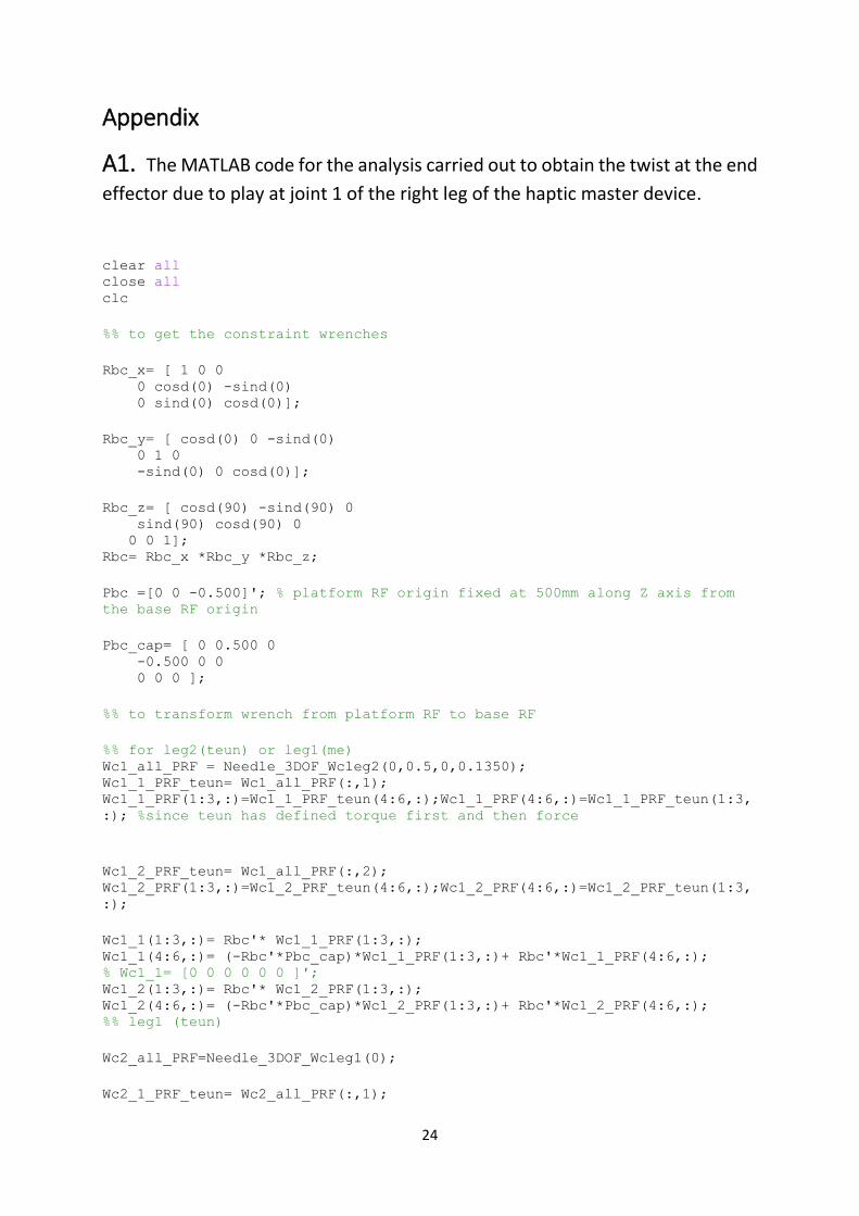
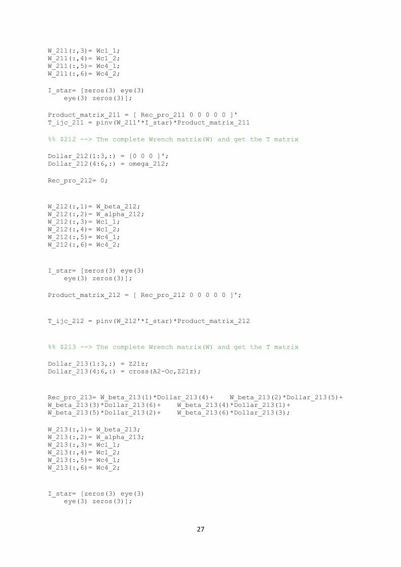
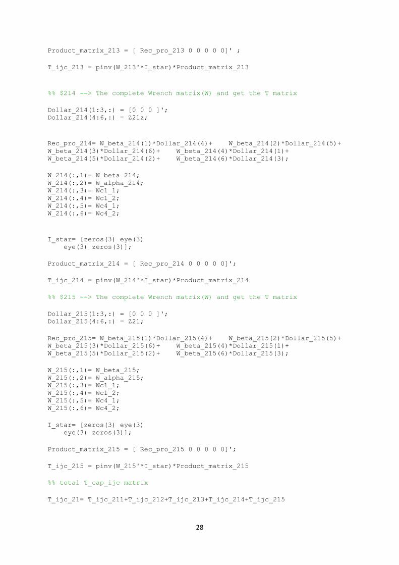
A1. The MATLAB code for the analysis carried out to obtain the twist at the end

effector due to play at joint 1 of the right leg of the haptic master device.

clear all close all clc

%% to get the constraint wrenches

Rbc_x= [ 1 0 0 0 cosd(0) -sind(0) 0 sind(0) cosd(0)];

Rbc_y= [ cosd(0) 0 -sind(0) 0 1 0 -sind(0) 0 cosd(0)];

Rbc_z= [ cosd(90) -sind(90) 0 sind(90) cosd(90) 0 0 0 1]; Rbc= Rbc_x *Rbc_y *Rbc_z;

Pbc =[0 0 -0.500]'; % platform RF origin fixed at 500mm along Z axis from

the base RF origin

Pbc_cap= [ 0 0.500 0 -0.500 0 0 0 0 0 ];

%% to transform wrench from platform RF to base RF

%% for leg2(teun) or leg1(me) Wc1_all_PRF = Needle_3DOF_Wcleg2(0,0.5,0,0.1350); Wc1_1_PRF_teun= Wc1_all_PRF(:,1); Wc1_1_PRF(1:3,:)=Wc1_1_PRF_teun(4:6,:);Wc1_1_PRF(4:6,:)=Wc1_1_PRF_teun(1:3,

:); %since teun has defined torque first and then force

Wc1_2_PRF_teun= Wc1_all_PRF(:,2); Wc1_2_PRF(1:3,:)=Wc1_2_PRF_teun(4:6,:);Wc1_2_PRF(4:6,:)=Wc1_2_PRF_teun(1:3,

:);

Wc1_1(1:3,:)= Rbc'* Wc1_1_PRF(1:3,:); Wc1_1(4:6,:)= (-Rbc'*Pbc_cap)*Wc1_1_PRF(1:3,:)+ Rbc'*Wc1_1_PRF(4:6,:); % Wc1_1= [0 0 0 0 0 0 ]'; Wc1_2(1:3,:)= Rbc'* Wc1_2_PRF(1:3,:); Wc1_2(4:6,:)= (-Rbc'*Pbc_cap)*Wc1_2_PRF(1:3,:)+ Rbc'*Wc1_2_PRF(4:6,:); %% leg1 (teun)

Wc2_all_PRF=Needle_3DOF_Wcleg1(0);

Wc2_1_PRF_teun= Wc2_all_PRF(:,1);

25

Wc2_1_PRF(1:3,:)=Wc2_1_PRF_teun(4:6,:);Wc2_1_PRF(4:6,:)=Wc2_1_PRF_teun(1:3,

:); %since teun has defined torque first and then force

Wc2_1(1:3,:)= Rbc'* Wc2_1_PRF(1:3,:); Wc2_1(4:6,:)= (-Rbc'*Pbc_cap)*Wc2_1_PRF(1:3,:)+ Rbc'*Wc2_1_PRF(4:6,:);


:);


%% for leg3(teun) or leg4(me)

Wc4_all_PRF= Needle_3DOF_Wcleg3(0);


:); %since teun has defined torque first and then force Wc4_1_PRF=[0 0 0 0 0 0 ]'; % to not consider the constraint along y axis in

leg 4 Wc4_2_PRF_teun= Wc4_all_PRF(:,2); Wc4_2_PRF(1:3,:)=Wc4_2_PRF_teun(4:6,:);Wc4_2_PRF(4:6,:)=Wc4_2_PRF_teun(1:3,

:);



%% to calculate the alpha and beta wrenches

A2 =[ 0.070 0 0]'; B2 = [ 0.135 0 0.500]'; Oc= [0 0 0 ]'; Ob = [ 0 0 0.500]';

Z21= [0 1 0 ]'; Z21z = [ 0 0 1]'; Z23= [0 1 0 ]'; Z24=[1 0 0 ]';

%% $211 wrenches

W_alpha_211= [0 0 0 0 0 0 ]';

omega_211= cross(Z21,Z21z)/sqrt(sum((cross(Z21,Z21z).*(cross(Z21,Z21z))))); W_beta_211(1:3,:) = Z23;

W_beta_211(4:6,:) = cross((B2-Oc),Z23);

26

%% $212 wrenches

omega_212= cross(Z21,Z21z)/sqrt(sum((cross(Z21,Z21z).*(cross(Z21,Z21z)))));

W_alpha_212(1:3,:) = Z23; W_alpha_212(4:6,:)= cross((B2-Oc),Z23);

W_beta_212 = [0 0 0 0 0 0 ]';

%% $213 wrenches

W_alpha_213= [ 0 0 0 0 0 0 ]';

W_beta_213(1:3,:) = Z23; W_beta_213(4:6,:)= cross((B2-Oc),Z23);

%% $214 wrenches

W_alpha_214(1:3,:)= Z23; W_alpha_214(4:6,:)= cross(B2-Oc,Z23);

W_beta_214= [0 0 0 0 0 0 ]';

%% $215 wrenches

omega_215= cross(Z23,Z24)/sqrt(sum((cross(Z23,Z24).*(cross(Z23,Z24)))));

W_alpha_215(1:3,:)= 0; W_alpha_215(4:6,:)= 0;

W_beta_215(1:3,:)= Z23; W_beta_215(4:6,:)= cross(B2-Oc,Z23);

%% individual virtual joint T matrices

%% $211 --> The complete Wrench matrix(W) and get the T matrix

Dollar_211(1:3,:) = omega_211; Dollar_211(4:6,:) = cross(A2-Oc,omega_211);

Rec_pro_211=

W_beta_211(1)*Dollar_211(4)+W_beta_211(2)*Dollar_211(5)+W_beta_211(3)*Dolla

r_211(6)+W_beta_211(4)*Dollar_211(1)+W_beta_211(5)*Dollar_211(2)+W_beta_211

(6)*Dollar_211(3);

W_211(:,1)= W_beta_211; W_211(:,2)= W_alpha_211;

27

W_211(:,3)= Wc1_1; W_211(:,4)= Wc1_2; W_211(:,5)= Wc4_1; W_211(:,6)= Wc4_2;

I_star= [zeros(3) eye(3) eye(3) zeros(3)];

Product_matrix_211 = [ Rec_pro_211 0 0 0 0 0 ]' T_ijc_211 = pinv(W_211'*I_star)*Product_matrix_211


Dollar_212(1:3,:) = [0 0 0 ]'; Dollar_212(4:6,:) = omega_212;

Rec_pro_212= 0;

W_212(:,1)= W_beta_212; W_212(:,2)= W_alpha_212; W_212(:,3)= Wc1_1; W_212(:,4)= Wc1_2; W_212(:,5)= Wc4_1; W_212(:,6)= Wc4_2;


Product_matrix_212 = [ Rec_pro_212 0 0 0 0 0 ]';

T_ijc_212 = pinv(W_212'*I_star)*Product_matrix_212


Dollar_213(1:3,:) = Z21z; Dollar_213(4:6,:) = cross(A2-Oc,Z21z);

Rec_pro_213= W_beta_213(1)*Dollar_213(4)+ W_beta_213(2)*Dollar_213(5)+

W_beta_213(3)*Dollar_213(6)+ W_beta_213(4)*Dollar_213(1)+

W_beta_213(5)*Dollar_213(2)+ W_beta_213(6)*Dollar_213(3);



28

Product_matrix_213 = [ Rec_pro_213 0 0 0 0 0]' ;



Dollar_214(1:3,:) = [0 0 0 ]'; Dollar_214(4:6,:) = Z21z;






Product_matrix_214 = [ Rec_pro_214 0 0 0 0 0]';



Dollar_215(1:3,:) = [0 0 0 ]'; Dollar_215(4:6,:) = Z21;






Product_matrix_215 = [ Rec_pro_215 0 0 0 0 0]';


%% total T_cap_ijc matrix

T_ijc_21= T_ijc_211+T_ijc_212+T_ijc_213+T_ijc_214+T_ijc_215

29

%% T matrix - with all T_cap_ijcs arranged in a matrix

T(:,1)= T_ijc_211; T(:,2)= T_ijc_212; T(:,3)= T_ijc_213; T(:,4)= T_ijc_214; T(:,5)= T_ijc_215

%% "A" matrix

A= T'*eye(6)*T;

%% find gmax

ri=0.000013; [V,D]=eig(A)

maxeigenvalue= max(max(D)) [num idx] = max(D(:)); [maxeigenidx maxeigenidy] = ind2sub(size(D),idx)

Vmax=V(:,maxeigenidy) gmax= ri.* Vmax

%% to find gopt

thetai= atan2(gmax(2),gmax(1)); thetaiplus1= atan2(gmax(4),gmax(3)); phii= atan2(sqrt(gmax(4)^2+gmax(3)^2),sqrt(gmax(2)^2+gmax(1)^2));

gopt(1)= ri*(cos(thetai)*cos(phii)); gopt(2)= ri*(sin(thetai)*cos(phii)); gopt(3)= ri*(cos(thetaiplus1)*sin(phii)); gopt(4)= ri*(sin(thetaiplus1)*sin(phii)); gopt(5)= sign(gmax(5)); gopt=gopt'

%% calculating optimal g

g=[0 0 0 0 0 ]'; for i= 1:size(diag(D))

g=g+ 0.000013*V(:,i);

end

g

%% calculating the final associated twist

finaltwist_ijc_211= g(3).*T_ijc_211; finaltwist_ijc_212= g(1).*T_ijc_212; finaltwist_ijc_213= g(4).*T_ijc_213; finaltwist_ijc_214= g(2).*T_ijc_214; finaltwist_ijc_215= g(5).*T_ijc_215;

30

finaltwist_ijc=

finaltwist_ijc_211+finaltwist_ijc_212+finaltwist_ijc_213+finaltwist_ijc_214

+finaltwist_ijc_215

T

A2. The result obtained after running the code:

Product_matrix_211 =

-0.5000

0

0

0

0

0

T_ijc_211 =

0.2000

-0.0000

-0.0000

-0.0000

-0.4000

0

T_ijc_212 =

31

0

0

0

0

0

0

T_ijc_213 =

-0.0260

0.0000

0.0000

0.0000

0.0520

0

T_ijc_214 =

0

0

0

0

0

0

32

T_ijc_215 =

-0.4000

0.0000

0.0000

0.0000

0.8000

0

T_ijc_21 =

-0.2260

0.0000

0.0000

0.0000

0.4520

0

T =

0.2000 0 -0.0260 0 -0.4000

-0.0000 0 0.0000 0 0.0000

33

-0.0000 0 0.0000 0 0.0000

-0.0000 0 0.0000 0 0.0000

-0.4000 0 0.0520 0 0.8000

0 0 0 0 0

V =

-0.8308 -0.1123 0 0.3128 -0.4465

0 0 -1.0000 0 0

0.1065 -0.9926 0 0.0093 0.0580

0.3466 0.0459 0 0.9369 0

-0.4223 0.0084 0 0.1558 0.8929

D =

-0.0000 0 0 0 0

0 -0.0000 0 0 0

0 0 0 0 0

0 0 0 0.0000 0

0 0 0 0 1.0034

maxeigenvalue =

34

1.0034

maxeigenidx =

5

maxeigenidy =

5

Vmax =

-0.4465

0

0.0580

0

0.8929

gmax =

1.0e-04 *

35

-0.0580

0

0.0075

0

0.1161

gopt =

-0.0000

0.0000

0.0000

0

1.0000

g =

1.0e-04 *

-0.1400

-0.1300

-0.1064

0.1728

0.0825

36

finaltwist_ijc =

1.0e-04 *

-0.0588

0.0000

0.0000

0.0000

0.1176

0

T =

0.2000 0 -0.0260 0 -0.4000

-0.0000 0 0.0000 0 0.0000

-0.0000 0 0.0000 0 0.0000

-0.0000 0 0.0000 0 0.0000

-0.4000 0 0.0520 0 0.8000

0 0 0 0 0

>>

Date post:	06-Mar-2018
Category:	Documents
Upload:	lamtu
View:	219 times
Download:	1 times

Internship Report - Universiteit Twenteessay.utwente.nl/69528/1/Internship Report Final_.pdf ·...

Documents