90
Ed. 310 – Assessment of Student Learning 1 CHAPTER 6
| Date post: | 14-Jul-2015 |
| Category: |
Education |
| Upload: | rica-joy-pontilar |
| View: | 235 times |
| Download: | 1 times |

Ed. 310 – Assessment of Student Learning 1CHAPTER 6


NORM-REFERENCED TESTS CRITERION-REFERENCED TESTS
1.Norm-referenced tests are used to determine theachievements of individuals in comparison with the achievements of other individuals who take the same test.
1. Criterion-referenced tests are used to determine the achievements of individuals in comparison with criterion, usually an absolute standard.
2. In a norm-referenced test, the quality of achievements of a student is determined by the distance of his score from the mean or median
2. In a criterion-referenced test, the quality of achievement of a student is determined by the distance of his score from the criterion established.
3. Norm-referenced tests are designed to produce variability among individuals.
3. In criterion-referenced tests, variability is irrelevant.

NORM-REFERENCED TESTS CRITERION-REFERENCED TESTS
4. Norm-referenced tests are used for selection and grouping purposes.
CRT are used to determine the level of skill or knowledge of individuals if they are capable of qualified to apply such skill or knowledge.
5. Norm Referenced Tests, non discriminating items such as items that are easy, too difficult and improved.
5. In a criterion-referenced test, too easy or too difficult items are not removed, rather they should be included if they truly reflect the skill being measured.


Relates to a point in a distribution around which the scores tend to center. This point can be used as the most representative value for a distribution of scores. A measure of central tendency is helpful in showing where the average or typical score fails.

Is the point or score at the midpoint of the distribution of scores arranged from highest to lowest or vice versa.

Calcula t ions of the Median for Ungrouped Score s
When the number cases are odd, arrange the scores from highest to lowest or vice versa. Write down all the scores, the median is the middlemost score.

Computat ion of the Median for Grouped Data
Given this frequency distribution/ grouped data X F90-94 185-89 280-84 775-79 970-74 11 65-69 860-64 555-59 550-54 145-49 1
N= 50

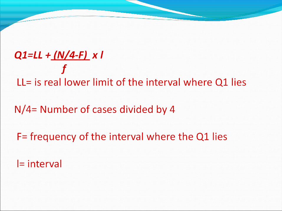
1. Use the formula (N/2- Fl)Mdn = LL + F x i
Where:LL= the real lower limit of the median classN/2=half sumF1= partial sumf= frequency of the class interval where the median liesN= the number of casesi= the interval

2. Find the values of the symbols: •N/2 = 50/2 = 25•FI = Add the frequencies of the score from the lower score end upward until reaching half sum but not exceeding it. (1 + 1 + 5 + 5 +8 =20). Twenty (20) is the partial sum from the lower limit. The median (25th score lies in the step-interval 70-74 and its frequency is 11)•The value off is 11 ( the frequency of the interval where the median lies)•LL is 69.9 ( the real lower limit of 70 – 74 = the interval where the median lies)•i, the interval of the class limits, is 5

3. Substitute the values for the symbols in the formula and solve. Mdn = 69.4 + (25-20) x 5
11 = 69.5 + 5 x 5 11
= 69.5 + (4545) x 5 = 69.5 + 2.2725Mdn = 71.77

4. Check the answer by using the formula: Mdn =UI – (N/2-Fu) x i
f
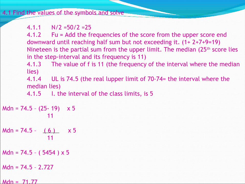
4.1 Find the values of the symbols and solve
4.1.1 N/2 =50/2 =254.1.2 Fu = Add the frequencies of the score from the upper score end downward until reaching half sum but not exceeding it. (1+ 2+7+9=19) Nineteen is the partial sum from the upper limit. The median (25th score lies in the step-interval and its frequency is 11)4.1.3 The value of f is 11 (the frequency of the interval where the median lies)4.1.4 UL is 74.5 (the real lupper limit of 70-74= the interval where the median lies)4.1.5 I. the interval of the class limits, is 5
Mdn = 74.5 – (25- 19) x 5
11 Mdn = 74.5 – ( 6 ) x 5
11 Mdn = 74.5 – ( 5454 ) x 5 Mdn = 74.5 – 2.727 Mdn = 71.77
The mean or the arithmetic mean is referred to as the average of scores or measures.

It considered the best measure of central tendency due to the following qualities:
1.Each score contributes its proportionate share in computing the mean. The mean is more stable than the median or the mode.2.Since the mean average, it is best understood and more widely used measure of central tendency3.It is used as basis in computing other statistical measures like the average deviation, standard deviation, coefficient of variability, coefficient of correlation, etc.

Computation of the Mean from Ungrouped Data (when the number of cases is less than
30)
1.Use the formula: M= ( The sum of X divided b y N )2.Write the scores in a column. They can be in any order.3.Count the number of scores to get N.4.Add the scores to get the sum5.Divide the sum by the number of cases.

The mean is:X68 M= 859/1770 M= 50.529 or 50.53564560546348352945633649365547

Computat ion of the Mean for Grouped Data
1. The formula in finding Mean for Grouped Data is:
X=AM + Where: AM = assumed mean = is the algebraic sum of the products of the frequencies and their corresponding deviations from the assumed mean N = the number of cases I = the class interval

2. Steps in the Computation of the Mean: 2.1 Prepare a table of frequency or frequency distribution. 2.2 Assume a mean. The assumed mean can be in any part of the frequency distribution, but it is advisable to get the midpoint of the class-interval at the middle of the distribution, that one highest frequency. 2.3 Fill column D starting from the step where the assumed mean lies, assign this a 0 deviation. Form 0, number the steps upward 1,2,3,4, and downward 1,2,3,4 etc. All deviations above the assumed mean have positive signs and all deviationsbelow the assumed mean have negative signs. 2.4 Multiply the frequency by the deviation for each step to get the fd column, and get sum of fd. This is the algebraic sum of the fd column. 2.5 Divide summation fd by N and multiply by the class interval x i 2.6 Add the product to the assumed mean 2.7 Check the answer by assuming another mean

Example: X f d fd 90-94 1 4 4 85-89 2 3 6 80-84 7 2 14 75-79 9 1 9 + 33 70-74 11 0 0 65-69 8 -1 -8 60-64 5 -2 -10 55-59 5 -3 -15 50-54 1 -4 -4
45-49 1 -5 -5 -42N = 50 Efd= -9

1. Assume a mean. Get the midpoint of the interval where the assumed mean lies.AM = 722. Fill in Column d (deviation). The deviation is the spread of the score from a point of origin.3. Fill in Column fd. The sum of the positive values is +33 and that of the negative values is -42. The sum of fd is -9.4. Substituting the formula:M = 72 + ( -9/50 ) 5M = 72 + ( -0.18 ) 5M = 72 + ( -0.9 )M = 72 + 0.9M = 71.10

5. Check your answer by assuming another mean X f d fd 90-94 1 5 5 85-89 2 4 8 80-84 7 3 21 75-79 9 2 18 70-74 11 1 11 + 63 65-69 8 0 -0 60-64 5 -1 -5 55-59 5 -2 -10 50-54 1 -3 -3
45-49 1 -4 -4 22N = 50 Efd + 41

Given:AM = 67Efd = + 41I = 5N = 50 M= 67 + (+41/50) 5M= 67 + (0.82) 5M= 67 + 4.1M= 71.10

Another method of computing the mean is through the midpoint method. The formula is: M= EFM N X f M fM 90-94 1 92 92 85-89 2 87 174 80-84 7 82 574 75-79 9 77 693 70-74 11 72 792 65-69 8 67 536 60-64 5 62 310 55-59 5 57 285 50-54 1 52 52
45-49 1 47 47 N= 50 EfM= 3555

Procedure:
1. Prepare a frequency distribution2. Place column M which represents the midpoints of each class interval3. Fill in Column Fm by multiplying each frequency by each corresponding midpoint4. Find the sum of the data in Column M5. Divide this by N.M = 3555/50 = 71.10

The mode is the most frequency occurring score in the distribution. It is the score with the highest frequency.

Determining the Mode from Ungrouped Score s ( Crude or Rough Mode )
Procedure:
1. Arrange the scores from highest to lowest2. The score that occurs most often is the crude mode.

Data:25 30 37 41 52 52 30 37 42 37 X 5252424137 Mode = 3737373730303025

Determining the Crude Mode from Grouped Score s (Frequency Dis t r ibut ion)
The crude mode is the midpoint of the interval with the highest frequency.

X F 90-94 1 85-89 2 80-84 7 75-79 9 70-74 11 Crude Mode = 72 65-69 8 60-64 5 55-59 5 50-54 1 45-49 1
N= 50

Computat ion of the True Mode
The formula for the True Mode is:Mo= 3Mdn- 2M
In which: Mo = the modeMdn = the medianM= the mean


The measures of location or point measures are the quartiles, deciles and percentiles are points dividing the distribution into les. The quartiles (Q1, Q2, Q3, and Q4) are points dividing the distribution into four equal parts. The percentiles (P1, P2, P3, etc) are points which divide the score distribution into one hundred equal parts.
The procedure in finding the point measures is almost the same as that of the median.

Quartiles
The first quartile (Q1) is located at one- fourth of the number of case, such as 25% of all the cases lie at or below it and 75% at or above it.
The value of third quartile corresponds to the value
of the seventy-percentile. Seventy-five percent of all the cases lie at or above it and 25% lie at or below it.
The value of the second quartile is equal to the value
of the median, such that 50%of all the cases lie at or below it and 50% lie at or above it.

Finding Q1 X F CM90-94 1 5085-89 2 4980-84 7 4775-79 9 4070-74 11 4065-69 8 2060-64 5 1255-59 5 750-54 1 245-49 1 1 N=50
Procedure:1. Add Column CM in the Frequency
Distribution. It stands for the cumulative frequencies, is done by adding the scores from the lower score end upward.
2. Find N/4. 50/4 = 12.5. The twenty-fifth score lies in the interval 65-69.
3. Determine the partial sum (F). That is the sum of the frequencies upward which totals 25 (Q/4) but not exceeding it. In the given distribution, the partial sum (F) is 12.
4. The value of f is 8 since it is the frequency of the interval where Q1 lies.
5. The value of LL or lower limit is 64.5.

Substituting the formula: Q1=64.5 + (12.5-12) x 5 8 Q1=64.5 + (0.5) x 5 8Q1=64.5 + (0.06) x 5Q1=64.5 + .30Q1= 64.80
Third Quartile Formula:Q3=LL + (3N-F) 4 l FLL= 74.5+ (37.5-31) x 5 9Q3=74.5 + (6.5/9) x5Q3=74.5 + (.72) x 5Q3= 74.5 + 3.6Q3= 78.1


Finding the Percentiles X F CM90-94 1 5085-89 2 4980-84 7 4775-79 9 4070-74 11 4065-69 8 2060-64 5 1255-59 5 750-54 1 245-49 1 1 N=50
Procedure:1.Determined the desired percentile.
E.g. P20.2.Find the percentile sum by
multiplying the number of cases (N) of 5 by the percentage desired 20% of 50=50 *.20=10
3.Find the partial sum by adding the frequencies of the scores from the lower score end upward until reaching the percentile sum but not exceeding it. (1+1+5=7. Percentile 20 or the 10th score lies at the interval 60-64.
4.Determine f= the frequency of 60-64 is 5.
5.Determine LL. The exact or real lower limit of 60-64 is 59.5
6.The interval is 5.


Introduction The measures of central tendency represented by the mean,
median and mode are valuable statistical measures, but they describe only the typical score representing the whole distribution. They describe only tendency of the scores to pile up or near the middle of the distribution. The measures of variability or dispersion are important. They show the tendency of the scores to spread or scatter above or below the central point of dispersion. They show how close or how far the scores are from each others. These measures also show the homogeneity or heterogeneity of different sets of scores. The higher the measure of variability the more homogenous is the group; the lower the measure of variability, the more heterogenous is the group. The most common measures or variability are the range, the standard deviation, the mean deviation and quartile deviation. The most important and most often used in measurement and research and in advanced statistics is the standard deviation.

Range
The range is the difference between the highest and lowest scores. It provides a quick approximation of the spread of the scores, but it is not a dependable measure of variability because it is calculated from only two values.Example: Highest Score =78; lowest score is 25. The range is 53.

Standard Deviation
The standard is the square root of the mean of the squared deviation of all scores from the mean. It is basically a measure of how far each score is from the mean. It is basically a measure of how far each score is from the mean. Since the standard deviation is based on deviations from the mean, these two statistics are used together to give meaning to test scores.
Computation of the Standard Deviation from Ungroup scores

Procedure:
List the scores under X column.Find the mean of the scores.Place column (deviations); get the values by subtracting the mean from each of the scores. When the scores are less than the mean, the negative sign precedes the difference between the raw score and the mean.Place column (); square each of the values.Find the sum of the squared deviation and divide it by the number of cases.

X 43 7 4941 5 2540 4 1638 2 437 1 133 -3 930 -6 3629 -7 4924 -12 14424 -12 14421 -15 225∑ X = 360 702 N= 10 X=36SD= SD= = 4.415

Mean Deviation or Average Deviation The mean deviation is not very much used in statistical work. Nevertheless, there are times when it becomes necessary to compute the mean or average deviation. The mean deviation is the square root of absolute values of the difference between the mean and the raw scores. MD= ∑/X-X/ N The symbol / / means that the signs are disregarded.

Example: X 43 7 41 5 40 4 38 2 37 1 33 -3 30 -6 29 -7 24 -12 24 -12 21 -15 ∑ X = 360 =74 N= 10 X=36 AM=74/10= 7.4

Standard Deviation from Group Scores
The formula for standard deviation using the short method is: SD= ______- _____ N N Where SD is standard deviation using the short method is: l is class interval ∑ is the sum of the products of the frequencies by the deviations of the score from the mean, squared. ∑ is the sum of the products of the frequencies by the deviations of the score from mean. N is the number of cases.

X F d fd 90-94 1 4 4 1685-89 2 3 6 1880-84 7 2 14 2875-79 9 1 9+33 970-74 11 0 0 065-69 8 -1 -8 860-64 5 -2 -10 2055-59 5 -3 -15 4550-54 1 -4 -4 1645-49 1 -5 -4 25 N=50 ∑ fd= -9 ∑=185
SD=5 SD= 5 SD= 5SD= 5SD= 5 x 1.9150SD= 9.575
Quartile Deviation (Q)
When using the statistics of percentiles, deciles, quartiles, or the median which are based on the scores, the standard deviation cannot be used as a measure of variability, since the deviation are based on the mean. The variability of distribution of scores can be used by using the two points, Q3 and Q1. A measure of the variability of the middle 50 percent of the scores is considered to be a good estimate, because extreme scores or erratic spacing between scores in the upper 25 percent and lower 25 percent are excluded in the computation. This is the quartile deviation. This is the value that is equal to the half the distance from Q1 to Q3.

Where: Q = quartile deviation Q3 =75th percentile Q1 = 25th percentile Finding the quartile deviation X F CM90-94 1 5085-89 2 4980-84 7 4775-79 9 4070-74 11 4065-69 8 2060-64 5 1255-59 5 750-54 1 245-49 1 1 N=50

Q1= 64.5+ (12.5-12) x 5 8Q1= 64.5 + (0.5) x5 8
Q1= 64.5 + (0.06) x 5Q1=64.5 + .30Q1=68.80

Third QuartileFormula: (3N-F) Q 3=LL+ 4 l
f3N/4 = 3 x 50 = 150/4 = 37.5
4 LL = 74.5F= 31f= 9I =5

Q3= 74.5 + (37.5-31) x 5 9
Q3 = 74.5 + (6.5/9) x 5 Q3= 74.5 + (.72) x 5Q3 = 74.5 + 3.6Q3 = 78.1 Q= 78.1 – 64 = 13.3
2


A standard score is one of many derived scores used in testing today. Derived scores are valuable to the classroom teacher. Since scores are differ from different tests, the teacher can make them comparable by expressing them in the same scale. For norm-referenced test, it is meaningful to interpret classroom test scores by locating a student’s score with reference to the average for the class and to describe the distance between the score and the average in terms of the spread of the scores in the distribution.

Tristan’s raw score on an English achievement test was 50. In the same class of students Tristan scored 70 on the Mathematics achievement test. To compare the raw score on one test with a raw score on another test to obtain a total or average score is meaningless. The units are not comparable because he tests may have different possible total scores, the units become comparable, and can be interpreted properly.

Using the deviation of a score from the mean (X – X) and the standard deviation (SD), a teacher can build what is called a z-score.
z=(X-M)/SD
Z= a standard score X= any raw score M= the mean SD= the standard deviation

For example, the means and standard deviation for Tristan’s two test scores are as follow: Tristan’s Raw Score Mean Standard
Deviation
English test 50 45 5.6Mathematics test 70 75 7

Comparison can be made between the two scores because the scores were earned in the same group of students.
Substituting the formula:
For English For Mathematics Z=(50-45)/5.6 Z=(70-75)/7 = 5/5.6 = .89 Z= -5/7 = -0.71

The two scores of Tristan can now be compared. Even if he got a higher score in mathematics than in English, he still did well in English as shown by the higher value of the standard score in that subject.


Skewness is the degree of symmetry of the scores.- Refers to the degree of symmetry attached to the occurrence of the scores along the score interval.

When the scores tend to center around one point with those on both sides of that point balancing each other, the distribution is said to have no skewness. If the atypical scores are above the measure of central tendency (in the positive direction), the distribution is said to be positively skewed. Likewise, if the atypical scores are below the measure of central tendency (in the negative direction), the distribution is said to be negatively skewed.

SK=(3 (M-Md))/SD

The characteristic of kurtosis is very closely related to the characteristics of variability. It can give an indication of the degree of homogeneity of the group being tested in regard to the characteristic being measured. if students tend to be much alike, the scores will generate a leptokurtic frequency polygon; if students are very different, a platykurtic distribution is generated. A mesokurtic distribution is neither platykurtic nor leptokurtic .

The kurtosis for the normal distribution is approximately 0.263. hence if the Ku is greater than 0.263, the distribution is most likely platykurtic; while if the Ku is less than 0.263, the distribution is most likely leptokurtic (Garett, 1973).
K=Q/((P90-P10))

Kurtosis is the degree of peakedness of a distribution. A normal disribion is a mesokric distribution. A pure leptokuric distribution has a higher peak than the normal distribution and has heavier tails. A pure platykurtic distribution has a lower peak than a normal distribution and lighter tails.


Most departures from normality display combinations of both skewness and kurtosis
different from a normal distribution.

Correlation is a measure of relationship or association between two or more paired variable or sets of data. The degree of correlation is indicated numerically by the correlation coefficient ® and graphically by a scotterplot. The r telis us the strength (weak or strong) and direction (negative or positive) of the relationship between distributions. The closer a coefficient gets to -1.0 or 1.0, the stronger the relationship. A perfect correlation is either -1.0 or + 1.0 and a complete lack of correlation is zero (0).

Computationsa. Scatterplot
The strength and direction of relationships between variable A and B can be determined by inspection with the use of a scatterplot. Consider the following:
Perfect Negative Correlation

Perfect Positive Correlation
Weak Negative Correlation

Weak Positive Correlation No Correlation

The Scotterplots in Different Directions
The scatterplots range from straight lines (perfect correlations) to ellipses (weaker correlations ) to circles (no correlations).
1. Spearman Rank Order Correlaion2.Pearson’s product-Moment Coefficient of correlation

Spearman Rank Order Correlation
Let us consider a relationship between learners’ rank in A and B subjects. The r is the easiest method of estimating relationship or ᵨassociation. Let us compute the following pairs of data using the Spearman rank order correlation (r ) starting from the raw score as ᵨfollows:
Learner A B A 85 60 B 80 65 C 78 70 D 75 66 E 70 72

Now, let us use the rank as follows:
Difference in Learner A B Rank (D) D² A 5 1 4 16 B 4 2 2 4 C 3 4 1 1 D 2 3 1 1 E 1 5 4 16
---------------- SD² = 38

To compute for rᵨ’ use this formula:
rᵨ = 1 - 6ED²/N (N²-1)where: rᵨ = rank difference correlation SD² = the sum of the squared difference between ranks N = number of learners
rᵨ = 1- 6(38)/ 5(25-1)= 1 – 228/ 5(24)= 1 – 228/ 120
= 1- 1.9= -0.9

The Spearman rank order correlation can be used with small number of cases, hence can be easily determined. It is acceptable for ordinal data only. Difference in rank (D) may carry a negative sign as in the case of 3- 4 = -1. However, since D is squared (D x D), it follows that negative times negative equals positive.

Pearson’s Product-Moment Coefficient of Correlation (r)
The Pearson’s- Product Moment Coefficient ® is
the most commonly used and the most precise coefficient of correlation. It may be calculated by converting the raw scores (Z) and finding the mean value of their products or by use of the raw score method.

Let us consider the raw score method between paired variables X and Y.
Learner X Y X²Y² Y² XY A 85 60 7225 3600 5100
B 80 65 6400 4225 5200 C 78 70 6084 4900 5460 D 75 66 5625 4356 4950 E 70 72 49005184 5040

The raw score method has five columns as illustrated above. To compute, follow the formula below:
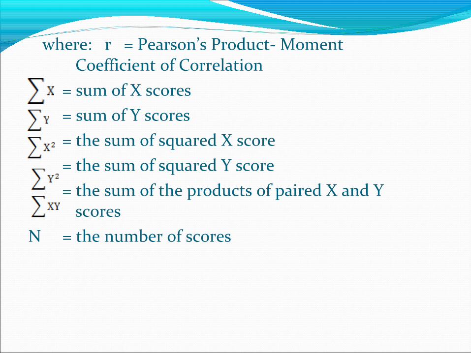
where: r = Pearson’s Product- Moment Coefficient of Correlation
= sum of X scores = sum of Y scores = the sum of squared X score = the sum of squared Y score = the sum of the products of paired X and Y
scoresN = the number of scores

=
= -0.87

The correlation value with the rank order method is – 0.9, while that with the raw score method is – 0.87. Correlations are interpreted in different ways. A crude method of interpreting the degree of correlation is shown below:
Coefficient ( r ) Relationship
± 0.00 to 0.20 Negligible ± 0.20 to 0.40 Low ± 0.40 to 0.60 Moderate ± 0.70 to 0.80 Substantial ± 0.80 to 1.00 High to very high


