Interpretation of dark-field contrast and particle-size selectivity in grating interferometers Susanna K. Lynch, 1 Vinay Pai, 1 Julie Auxier, 2 Ashley F. Stein, 3 Eric E. Bennett, 1 Camille K. Kemble, 1 Xianghui Xiao, 4 Wah-Keat Lee, 4 Nicole Y. Morgan, 1 and Han Harold Wen 1, * 1 Lab of Imaging Physics, Translational Medicine Branch, National Heart, Lung and Blood Institute, National Institutes of Health, Bethesda, Maryland 20892, USA 2 School of Chemical, Biological and Environmental Engineering, Oregon State University, Corvallis, Oregon 97331, USA 3 Harvard Medical School, Boston, Massachusetts 02115, USA 4 X-Ray Science Division, Advanced Photon Source, Argonne National Laboratory, Argonne, Illinois 60439, USA *Corresponding author: [email protected]Received 18 April 2011; revised 2 June 2011; accepted 2 June 2011; posted 6 June 2011 (Doc. ID 145968); published 22 July 2011 In grating-based x-ray phase sensitive imaging, dark-field contrast refers to the extinction of the inter- ference fringes due to small-angle scattering. For configurations where the sample is placed before the beamsplitter grating, the dark-field contrast has been quantified with theoretical wave propagation mod- els. Yet when the grating is placed before the sample, the dark-field contrast has only been modeled in the geometric optics regime. Here we attempt to quantify the dark-field effect in the grating-before-sample geometry with first-principle wave calculations and understand the associated particle-size selectivity. We obtain an expression for the dark-field effect in terms of the sample material’s complex refractive index, which can be verified experimentally without fitting parameters. A dark-field computed tomogra- phy experiment shows that the particle-size selectivity can be used to differentiate materials of identical x-ray absorption. OCIS codes: 340.7450, 170.7440, 340.7460. 1. Introduction Grating-based x-ray phase sensitive imaging techni- ques generally employ a grating in the x-ray beam to produce a dense fringe pattern on the image plane at some distance downbeam; changes in the position and amplitude of the fringes indicate x-ray refraction and coherent scattering in the sample (Fig. 1)[1–8]. The advantage of the grating approach is its ability to acquire full-field images using gratings of large areas. X-ray refraction and diffraction both arise from spatial variation of the refractive index in the sample material, but on different length scales. X-ray refraction is caused by macroscopic variations of the refractive index in the sample that are resolved by the imaging detector. Diffraction, or coherent scat- tering, is caused by unresolved, microscopic fluctua- tions of the refractive index. Coherent scattering causes angular divergence of the incident beam, which is observed in diffraction-enhanced imaging [9] and rigorously modeled by Nesterets [10]. In grating-based techniques, the scattering effect incurs a drop of the fringe amplitude in addition to the usual intensity attenuation caused by absorp- tion. The additional fringe amplitude attenuation is represented by the dark-field image [6]. We showed in a previous paper that the fringe amplitude decays exponentially with the sample thickness in the geometric optics regime [7], and Yashiro et al. showed the same relationship in the Talbot interferom- eter configuration with the sample proceeding the 4310 APPLIED OPTICS / Vol. 50, No. 22 / 1 August 2011
Transcript
Interpretation of dark-field contrast and particle-sizeselectivity in grating interferometers
Susanna K. Lynch,1 Vinay Pai,1 Julie Auxier,2 Ashley F. Stein,3 Eric E. Bennett,1
Camille K. Kemble,1 Xianghui Xiao,4 Wah-Keat Lee,4
Nicole Y. Morgan,1 and Han Harold Wen1,*1Lab of Imaging Physics, Translational Medicine Branch, National Heart, Lung and Blood Institute,
National Institutes of Health, Bethesda, Maryland 20892, USA2School of Chemical, Biological and Environmental Engineering, Oregon State University,
Corvallis, Oregon 97331, USA3Harvard Medical School, Boston, Massachusetts 02115, USA
4X-Ray Science Division, Advanced Photon Source, Argonne National Laboratory,Argonne, Illinois 60439, USA
Received 18 April 2011; revised 2 June 2011; accepted 2 June 2011;posted 6 June 2011 (Doc. ID 145968); published 22 July 2011
In grating-based x-ray phase sensitive imaging, dark-field contrast refers to the extinction of the inter-ference fringes due to small-angle scattering. For configurations where the sample is placed before thebeamsplitter grating, the dark-field contrast has been quantified with theoretical wave propagationmod-els. Yet when the grating is placed before the sample, the dark-field contrast has only beenmodeled in thegeometric optics regime. Here we attempt to quantify the dark-field effect in the grating-before-samplegeometry with first-principle wave calculations and understand the associated particle-size selectivity.We obtain an expression for the dark-field effect in terms of the sample material’s complex refractiveindex, which can be verified experimentally without fitting parameters. A dark-field computed tomogra-phy experiment shows that the particle-size selectivity can be used to differentiate materials of identicalx-ray absorption.OCIS codes: 340.7450, 170.7440, 340.7460.
1. Introduction
Grating-based x-ray phase sensitive imaging techni-ques generally employ a grating in the x-ray beam toproduce a dense fringe pattern on the image plane atsome distance downbeam; changes in the positionand amplitude of the fringes indicate x-ray refractionand coherent scattering in the sample (Fig. 1) [1–8].The advantage of the grating approach is its abilityto acquire full-field images using gratings of largeareas. X-ray refraction and diffraction both arisefrom spatial variation of the refractive index in thesample material, but on different length scales.X-ray refraction is caused by macroscopic variationsof the refractive index in the sample that are resolvedby the imaging detector. Diffraction, or coherent scat-
tering, is caused by unresolved, microscopic fluctua-tions of the refractive index. Coherent scatteringcauses angular divergence of the incident beam,which is observed in diffraction-enhanced imaging[9] and rigorously modeled by Nesterets [10].
In grating-based techniques, the scattering effectincurs a drop of the fringe amplitude in addition tothe usual intensity attenuation caused by absorp-tion. The additional fringe amplitude attenuation isrepresented by the dark-field image [6]. We showedin a previous paper that the fringe amplitude decaysexponentially with the sample thickness in thegeometric optics regime [7], and Yashiro et al. showedthe same relationship in the Talbot interferom-eter configuration with the sample proceeding the
beamsplitter grating [sample-before-grating (SbG)configuration] [11]. The fringe amplitude has alsobeen modeled phenomenologically in dark-field com-puted tomography (CT) [12,13]. Specifically, if A isthe fringe amplitude without any sample, and A0 isthe fringe amplitude when a sample of a singlematerial and thickness T is in the beam, then theabove models state that
A0=A ¼ expð−μaT − μdTÞ; ð1Þ
where μa is the absorption coefficient of the materialand μd is the dark-field extinction coefficient (DFEC).The DFEC accounts for the effect of small-angle scat-tering on the fringes and is, by definition, the extinc-tion coefficient of the fringe visibility V. The visibilityis defined as the ratio of the fringe amplitude A overthe average intensity J:
V ¼ A=J: ð2Þ
The above relationship is illustrated in Fig. 2.In coherent scattering, both the cross section and
the angular distribution are dependent on the lengthscale of the scattering structures, so the dark-fieldextinction can potentially be used to characterizematerials containingmicroscattering structures [14].We showed in previous works [7,15] that the fringevisibility decays exponentially with the samplethickness when the fringes are geometric projectionsof Ronchi-type gratings and that the DFEC is deter-mined by an autocorrelation of the electron densitydistribution. The correlation distance is determinedby the device settings. In cases where wave interfer-
ence must be considered, Yashiro et al. [11] analyzedTalbot interferometers in the SbG configuration[Fig. 1(a)]. They showed the exponential relationshipwith rigorous wave calculations, and they obtainedthe expression of the DFEC in terms of the autocor-relations of the complex refractive index.
An essential assumption shared by the Yashiroet al. model and the earlier Nesterets model is thatthe sample is illuminated by a plane wave. Underthis assumption, the complex wave at any point onthe wavefront can be expressed as a single-path in-tegral through the sample along the direction of thebeam. However, in the grating-before-sample (GbS)configuration with the grating proceeding the sample[16], the plane wave assumption no longer holds. Thesample is now illuminated by a sum of plane waves atdifferent angles. The transmitted wave involves thesum of projections along different paths in the sam-ple. As a result, the derivations of Nesterets and Ya-shiro cannot be easily extended to obtain the DFEC.
Because the GbS geometry has certain practicaladvantages over the SbG geometry, it is worthwhileto obtain the DFEC for the GbS geometry. These ad-vantages include the ease of grating fabrications [16]and lower radiation exposure when Ronchi-type in-tensity gratings are used [7,15,17–19]. We thereforeobtained the theoretical expression of the DFEC forthe GbS geometry using a stacked-slice model andwave propagation calculations.
The theoretical expression was then tested inaqueous suspensions of silica microspheres. In a 3Dtomography experiment of iron-oxide particle suspen-sions, the dark-field image is shown to distinguish be-tween materials of different microscopic compositionbut similar bulk absorption coefficients [20].
2. Theory of the GbS Geometry Dark-Field ExtinctionCoefficient
Our starting assumptions are the same as the onesby Nesterets and Yashiro, but without the planewave assumption. These are (i) the short wavelengthassumption—over the distance of the x-ray wave-length λ, the phase and absorption effects in thematerial are small and (ii) the small angle scattering
Fig. 1. Two different configurations of grating interferometers.(a) In the SbG geometry, a plane wave illuminates the sampleand then the gratings. (b) In the GbS geometry, the plane waveis split by the grating into different directions of propagationand then transmitted through the sample.
Fig. 2. Illustration of the fringe amplitude A and averageintensity J of a fringe pattern on the detector screen. The fringevisibility V is defined as A=J.
assumption—if the typical size of the unresolvedscatterers in the material is D, then λ=D ≪ 1.
We denote the complex refractive index of theimaged sample as
n ¼ 1þ χ; ð3Þ
where
χ ¼ −δ − iβ; ð4Þ
where δ and β represent the phase shifts and magni-tude attenuation in the material, respectively. Theshort wavelength assumption means that jχj ≪ 1.We consider χ to contain a smooth (resolvable) partχs and a fine (unresolved) part χf [10]:
Let the incident beam come along the Z axis. Ourbasic model is to section the sample into a stack ofthin slices of thickness t, along planes perpendicularto the Z axis (Fig. 3). Removing all material beyondthe plane at z allows us to consider the incrementaleffect of a single slice t. We denote the fringe ampli-tude on the detector before adding the slice as AðzÞ,and after as Aðzþ tÞ. The average intensities on thedetector before and after adding the slice are denotedas JðzÞ and Jðzþ tÞ. The fringe visibility V is definedas the ratio A=J. If V to the leading order of t satisfies
Vðzþ tÞ − VðzÞ ¼ −tμdðzÞVðzÞ; ð8Þ
and μd is a parameter expressed in the fine fluctua-tion χf , then the differential form of Eq. (8) is
dVðzÞdz
¼ −μdðzÞVðzÞ: ð9Þ
The solution to this equation is simply
VðzÞ ¼ Vð0Þ exp�−
Zz
0μdðτÞdτ
�: ð10Þ
Equation (10) would mean that the fringe visibilitydecreases exponentially with the sample thicknessby the coefficient μd, which is the DFEC that we wantto solve.
To carry out this procedure, we first focus on thecomplex wave function at the entry plane z of the thinslice (the entry wave function) (see Fig. 3) and thecomplex wave function at the exit plane zþ t (exitwave function). The entry wave function is an inte-gral sum of plane waves of a spread of wave vectork’s. By the small-angle scattering assumption,kx=k ≪ 1 and ky=k ≪ 1. We denote the complex am-plitude of wave vector (kx, ky, kz) as aðkx; kyÞ, so thatthe entry wave function is
Eðx; y; zÞ ¼Z
dkxdkyaðkx; kyÞ expð−ikxx − ikyy − ikzzÞ:ð11Þ
The exit wave function can be expressed in terms ofthe entry wave function by the projection approxima-tion under the short wavelength assumption [21]:
Eðx;y;zþ tÞ¼Z
dkxdkyaðkx;kyÞexpð−ikxx− ikyy− ikzzÞ
×exp½−iΦðkx;ky;x;y;zÞ�; ð12Þ
where Φ is the phase delay and attenuation throughthe slice for each plane wave along its path:
Φðkx; ky; x; y; zÞ ¼Z
t
0dτ k
2
kzχ�x −
kxkτ; y − ky
kτ; zþ τ
�:
ð13Þ
Because we model the refractive index χ as the sumof smooth and fine parts [Eq. (5)],Φ also contains twoparts:
Now we expand χf to the leading order of kx=kand ky=k:
Fig. 3. To model the DFEC in the GbS geometry, the imagedsample is sectioned into thin slices along the Z axis. The effectof a slice of thickness t at position z is analyzed by first removingall material beyond z, and then adding only the slice. The gap be-tween the two surfaces of the section plane at z is artificially addedto illustrate the entry wave into the slice.
Under the small-angle scattering assumption, if thetypical size of the fluctuations in the fine part of therefractive index χf is D, then
kxk;kyk∼
λD
≪ 1: ð17Þ
Substituting Eq. (17) into Eq. (16), and noting thatthe spatial derivatives of χf in the X and Y directionsare on the order of χf =D, while τ is between 0 and t,we have
χf�x−
kxkτ;y−ky
kτ;zþ τ
�¼ χf ðx;y;zþ τÞ
�1þO
� λtD2
��;
ð18Þ
where Oðλt=D2Þ means a term on the order of λt=D2.Additionally, the k2=kz factor in Eq. (13) can beexpanded by the Taylor series as
k2
kz≈ k
�1þ 1
2
�k2x þ k2y
k2
��¼ k
�1þO
� λ2D2
��: ð19Þ
Substituting Eqs. (18) and (19) into Eq. (15) yields
Φf ðkx; ky; x; y; zÞ ¼Z
t
0dτkχf ðx; y; zþ τÞ
�1þO
� λ2D2
�
þO
� λtD2
��: ð20Þ
Now we can make the slice thickness t small enoughsuch that jχf jkt ≪ 1 and λt=D2
≪ 1, then
Φf ðkx; ky; x; y; zÞ ≈ Φf ðx; y; zÞ; ð21Þ
where
Φf ðx; y; zÞ ¼ kZ
t
0dτχf ðx; y; zþ τÞ: ð22Þ
Equation (22) means that in a thin slice and underthe small-angle scattering assumption, the projec-tion through the slice for the different plane wavescan be approximated by a single projection alongthe Z direction.
We now substitute Eq. (21) into Eq. (14) and theresult into Eq. (12) to simplify the expression ofthe wave on the exit plane:
Note that if the fine part χf did not exist in the sliceand only the smooth χs is present, then the exit wavefunction would be
Esðx;y;zþ tÞ¼Z
dkxdkyaðkx;kyÞexpð−ikxx− ikyy− ikzzÞ
×exp½−iΦsðkx;ky;x;y;zÞ�: ð24Þ
So Eq. (23) means that the actual exit wave functionwith both χf and χs present can be expressed as amodification on the smooth wave function Es (notethat Es still accounts for χf in the sample up tothe entry plane of the slice):
We are now ready to calculate the fringe amplitudeon the detector plane at position zd. For horizontalfringes, the fringe amplitude is defined as
A ¼ 2Area
Zdetector
dxddydIð~rdÞ expð−igydÞ; ð26Þ
where “Area” is the detector area illuminated byx rays, IðrdÞ is the x-ray intensity at position rd onthe detector plane, and g ¼ 2π=ðfringe periodÞ. Theintensity IðrdÞ is given by the wave function on thedetector plane:
Ið~rdÞ ¼ Eð~rdÞE�ð~rdÞ: ð27Þ
We write the wave function on the detector planeEðrdÞ in terms of the wave function on the exit planeof the thin slice EðrÞ by a propagator P:
Eð~rdÞ ¼Zzplane
dxdyEð~rÞPð~rd −~rÞ: ð28Þ
Substituting Eq. (28) into Eq. (27) and the result intoEq. (26) gives an expression of the fringe amplitudein terms of the wave function at the exit plane:
Now we need to find an explicit form for the functionQ in order to calculate the fringe amplitude. Underthe small-angle scattering assumption expressed inEq. (17), we use the Fresnel–Kirchhoff diffractionformula for the propagator P [22]:
Pð~rd −~rÞ ¼−iλexpð−ikj~rd −~rjÞ
j~rd −~rj: ð31Þ
We now expand the propagator P with theFresnel formula under the small-angle scatteringassumption:
Pð~rd −~rÞ ≈−iλ
1ðzd − zÞ exp
�−ikðzd − zÞ − ik
1Zd − z
×�x2d þ y2d þ x2 þ y2
2− xdx − ydy
��; ð32Þ
and we substitute this back into Eq. (30) to obtain
Qð~r1;~r2Þ ¼1
Area
Zdetector
dxddyd1
λ2ðzd − zÞ2
× exp�−ik
1zd − z
�x21 þ y21 − x22 − y22
2
− xdðx1 − x2Þ − ydðy1 − y2 − dÞ��
; ð33Þ
where the distance d is given in terms of the fringeperiod p as
d ¼ gkðzd − zÞ ¼ λ
pðzd − zÞ: ð34Þ
Integrating Eq. (33) over the xd and yd on the detec-tor plane results in a simple expression for Q:
Qð~r1;~r2Þ ¼1
Areaδðx1 − x2Þδðy1 − y2 − dÞ
× exp�−ig
�y2 þ
d2
��: ð35Þ
By substituting Eq. (35) into Eq. (29), we obtain theexpression of the fringe amplitude in terms of the en-try wave function before the slice is added:
AðzÞ ¼ 2Area
Zzplane
dxdyE�~rþ d
2y
�E�
�~r −
d2y
�
× expð−igyÞ: ð36Þ
After adding the slice, the fringe amplitude can bewritten in terms of the exit wave function in the sameway:
Aðzþ tÞ ¼ 2Area
Zzþtplane
dxdyE�x; yþ d
2; zþ t
�
× E��x; y −
d2; zþ t
�expð−igyÞ: ð37Þ
Substituting the expression of the exit wave functionin Eq. (25) into Eq. (37) leads to
Aðzþ tÞ ¼ 2Area
Zzþtplane
dxdy exp�−iΦf
�x; yþ d
2; z
�
þ iΦf��x; y −
d2; z
��Es
�x; yþ d
2; zþ t
�
× Es��x; y −
d2; zþ t
�expð−igyÞ: ð38Þ
Next, we define
ΔΦf ðx; y; zÞ ¼ Φf
�x; yþ d
2; z
�−Φf
��x; y −
d2; z
�:
ð39Þ
Because we have made the slice thickness t suffi-ciently small such that jχf jkt ≪ 1, by Eq. (20) we haveΔΦf ðx; y; zÞ ≪ 1. Therefore, we write the Taylor ser-ies of Aðzþ tÞ in Eq. (38) in terms of ΔΦf ðx; y; zÞ:
Aðzþ tÞ ≈ 2Area
Zzþtplane
dxdy½1 − iΔΦf ðx; y; zÞ
−12ΔΦ2
f ðx; y; zÞ�Es
�x; yþ d
2; zþ t
�Es
�
�x; y −
d2; zþ t
�expð−igyÞ: ð40Þ
The leading term of the Taylor series in Eq. (40) is
Asðzþ tÞ ¼ 2Area
Zzþtplane
dxdyEs
�x; yþ d
2; zþ t
�Es
�
�x; y −
d2; zþ t
�expð−igyÞ: ð41Þ
With Eq. (36) we recognize Asðzþ tÞ as the fringe am-plitude we would get if the slice only contained thesmooth variation χs. This is a very useful fact inthe following derivation.
The second term in the Taylor series of Eq. (40) is
ΔA1 ¼ −i2
Area
Zzþt plane
dxdyΔΦf ðx; y; zÞ
× Es
�x; yþ d
2; zþ t
�Es
�
�x; y −
d2; zþ t
�expð−igyÞ: ð42Þ
Because ΔΦf ðx; y; zÞ is proportional to the fine fluc-tuation χf in the slice, and Es contains only the
smooth χs in the slice, the spatial fluctuation ofΔΦf ðx; y; zÞ is random relative to the rest of the inte-grand in Eq. (42). Therefore, only the average ofΔΦf ðx; y; zÞ in the XY plane contributes to the inte-gral. If we denote the average in the XY plane as<>xy, then
ΔA1 ¼ −i < ΔΦf ðx; y; zÞ >xy2
Area
Zzþtplane
dxdy
× Es
�x; yþ d
2; zþ t
�
× Es��x; y −
d2; zþ t
�expð−igyÞ: ð43Þ
Using the expression of Asðzþ tÞ in Eq. (41),Eq. (43) is shortened to
ΔA1 ¼ −i < ΔΦf ðx; y; zÞ >xy Asðzþ tÞ: ð44Þ
Because < χf >xy¼ 0, we have
< ΔΦf ðx; y; zÞ >xy¼ 0: ð45Þ
Therefore,
ΔA1 ¼ 0: ð46Þ
The last term of the Taylor series in Eq. (40) is
ΔA2 ¼ −1
Area
Zzþt plane
dxdyΔΦ2f ðx; y; zÞ
× Es
�x; yþ d
2; zþ t
�Es
�
�x; y −
d2; zþ t
�expð−igyÞ: ð47Þ
Again by the same reasoning leading to Eq. (43), wehave
ΔA2 ¼ − < ΔΦ2f ðx; y; zÞ >xy
×1
Area
Zzþtplane
dxdyEs
�x; yþ d
2; zþ t
�Es
�
�x; y −
d2; zþ t
�expð−igyÞ: ð48Þ
Using Eq. (41), Eq. (48) is shortened to
ΔA2 ¼ −12< ΔΦ2
f ðx; y; zÞ >xy Asðzþ tÞ: ð49Þ
From the definition of ΔΦf ðx; y; zÞ in Eq. (39) andthe definition of Φf ðx; y; zÞ in Eq. (22), we can furtherwrite
< ΔΦ2f ðx; y; zÞ >xy¼ k2 <
�Zt
0dτ1χf ðx; yþ
d2; zþ τ1Þ
−
Zt
0dτ2χf �
�x; y −
d2; zþ τ2
��2>xy : ð50Þ
We define a function Cðd; zÞ as
Cðd; zÞ ¼ 12t
<
�Zt
0dτ1χf
�x; yþ d
2; zþ τ1
�
−
Zt
0dτ2χf �
�x; y −
d2; zþ τ2
��2>xy; ð51Þ
then Eq. (50) is shortened to
< ΔΦ2f ðx; y; zÞ >xy¼ 2k2Cðd; zÞ: ð52Þ
Substituting Eq. (52) into Eq. (49) yields
ΔA2 ¼ −tk2Cðd; zÞAsðzþ tÞ: ð53Þ
Finally, we collect all three terms in the Taylor seriesin Eq. (40) to obtain an expression of the fringe am-plitude after the addition of the thin slice:
Aðzþ tÞ ¼ Asðzþ tÞ½1 − tk2Cðd; zÞ�: ð54ÞTo calculate the fringe visibility V, we still need
to find the expression for the average intensity Jon the detector plane. The average intensity on thedetector is
J ¼ 1Area
Zdetector
dxddydIð~rdÞ: ð55Þ
From Eq. (26) we recognize that the average inten-sity is equivalent to half of a hypothetical fringe am-plitude when the fringe period is infinitely large.Correspondingly, the distance d defined in Eq. (34)is zero. So, the same expression derived for the fringeamplitude in Eq. (54) also applies to the intensity ex-cept that the distance d is now zero:
Jðzþ tÞ ¼ Jsðzþ tÞ½1 − tk2Cð0; zÞ�: ð56Þ
The fringe visibility after the addition of the slice is,by definition, Vðzþ tÞ ¼ Aðzþ tÞ=Jðzþ tÞ. Substitut-ing Eq. (56) and (54) into this definition yields
Vðzþ tÞ ¼ Asðzþ tÞJsðzþ tÞ
½1 − tk2Cðd; zÞ�½1 − tk2Cð0; zÞ�
≈ Vsðzþ tÞf1 − tk2½Cðd; zÞ − Cð0; zÞ�g; ð57Þ
where Vsðzþ tÞ is the fringe visibility if the refractiveindex of the slice only contains the smooth part χs.Because the smooth part is resolved by the detectorand does not alter the fringe visibility, Vsðzþ tÞ isequal to the fringe visibility before adding the slice:
In differential form, this equation is equivalent to
dVðzÞdz
¼ −k2½Cðd; zÞ − Cð0; zÞ�VðzÞ; ð61Þ
and the solution is
VðzÞ ¼ Vð0Þ exp�−
Zz
0k2½Cðd; τÞ − Cð0; τÞ�dτ
�: ð62Þ
Thus we finally showed that in the GbS geometry, thefringe visibility also decreases exponentially with thesample thickness and the extinction coefficient at lo-cation z in the sample is
μdðzÞ ¼ k2½Cðd; zÞ − Cð0; zÞ�: ð63ÞTo express the DFEC in terms of the complex re-
fractive index of the material χ, we substitute the de-finition of CðdÞ in Eq. (51) into Eq. (63) to obtain
μdðzÞ ¼k2
2t<
�Zt
0dτ1χf
�x; yþ d
2; zþ τ1
�
−
Zt
0dτ2χf �
�x; y −
d2; zþ τ2
��2
−
�Zt
0dτ1χf ðx; y; zþ τ1Þ
−
Zt
0dτ2χf �ðx; y; zþ τ2Þ
�2>xy
¼ k2�1t<
Zt
0dτ1
Zt
0dτ2χf ðx; y; zþ τ1Þ
× χf �ðx; y; zþ τ2Þ >xy −1t
<
Zt
0dτ1
Zt
0dτ2χf
�x; yþ d
2; zþ τ1
�
× χf ��x; y −
d2; zþ τ2
�>xy
�: ð64Þ
We define an autocorrelation function of the fine partof the complex refractive index χf as
Rðd; zÞ ¼ 1t<
Zt
0dτ1
Zt
0dτ2χf
�x; yþ d
2; zþ τ1
�
× χf ��x; y −
d2; zþ τ2
�>xy; ð65Þ
where d is the autocorrelation distance. Then, thefinal reduced expression of the DFEC is
μdðzÞ ¼4π2λ2 ½Rð0; zÞ − Rðd; zÞ�: ð66Þ
Experimentally, if the sample is made of a singletype of material, then the DFEC is the same overthe sample. It can be measured from the fringe vis-ibility with the sample present (V 0) and without thesample (V):
μd ¼ −1TlnðV 0=VÞ; ð67Þ
where T is the thickness of the sample.
3. Applying to a Suspension of Microspheres ofUniform Diameter
We applied the above theory to obtain the DFEC of arandom suspension of silica microspheres of diam-eter D in water. If the distance between the sampleand the detector is L and the fringe period is p, thenthe autocorrelation distance d defined by Eq. (34) isλL=p. If we denote the difference of the complex re-fractive index between silica and water as Δχ, thenEqs. (66) and (65) lead to a closed-form expression ofthe DFEC:
where f is the volume fraction of the microspheresand D0 is the ratio D=d.
For hard x rays, the difference between the com-plex refractive indices of two materials is determinedby the difference in the electron density Δρ and ab-sorption coefficient Δμ:
Δχ ¼ −reλ2Δρ=2π − iλΔμ=2π; ð69Þ
where re is the classical electron radius of2:82 × 10−15 m. Because both Δρ and Δμ are known,the DFEC can be evaluated directly from Eq. (68)and verified experimentally without any fittingparameters.
4. Experimental Test of the Theory
The experiments were performed at beamlines 32-IDand 2-BM of the Advanced Photon Source (APS)at the Argonne National Laboratory, Argonne, Ill.Four samples of microsphere suspensions wereimaged, each containing 10 μm uniform silica micro-spheres of 2:0 g=cm3 density and 0.15, 0.3, 0.5 or
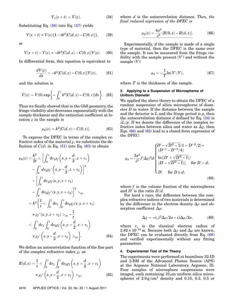
1:5 μm diameters, separately. The experimental con-ditions are tabulated in Table 1. The samples wereheld in 0:5ml centrifuge vials. The size of the x-raybeams were approximately 1:0mm. Each vial was po-sitioned, in turn, to center on the beam and imaged.On the 32-ID beamline, the 15 μm fringes were pro-duced with a custom-fabricated silicon π=2 phaseshift grating of 15 μm period. The grating was placedat one-fourth the Talbot distance from the detector.On the 2-BM beamline, a two-dimensional cross-gridRonchi grating was used to produce the 78 μm fringes[23]. The Ronchi grating was a geological sieve wovenof gold wires.
To obtain theoretical values of the DFEC fromEq. (68), the volume fraction f of the microspheresin a sample was determined from the measured in-tensity attenuation coefficient μ and the publishedvalues of water and silica by the United States Na-tional Institute of Standards and Technology (http://physics.nist.gov/PhysRefData/FFast/html/form.html):
f ¼ ðμ − μwaterÞ=ðμsilica − μwaterÞ: ð70Þ
In order to plot data from different x-ray energiesand microsphere diameters on the same graph, wecalculated the normalized and unitless DFEC, whichwe define as
μd0 ¼ μdλ2=ð3π2f jΔχj2dÞ: ðd71Þ
By Eq. (68) μd0 is only dependent on D0, which is theratio of the microsphere diameter over the autocorre-lation distance. We can therefore plot all data on a μd0versus D0 graph.
The experimental values of the DFEC were com-puted from the fringe visibility according to Eq. (67).The fringe visibility was computed from the fringeamplitude according to its definition of (fringe ampli-tude)/(average intensity). The fringe amplitude andaverage intensity were in turn measured from theraw images according to Eq. (26) [7,15].
5. Results
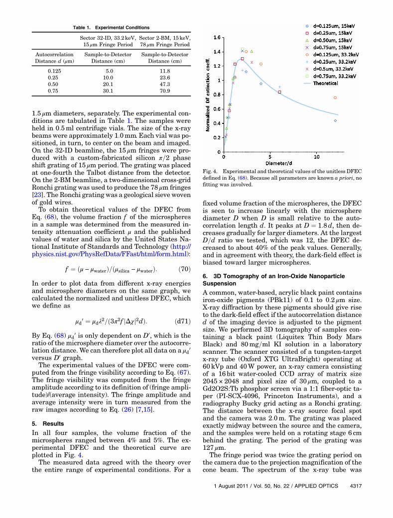
In all four samples, the volume fraction of themicrospheres ranged between 4% and 5%. The ex-perimental DFEC and the theoretical curve areplotted in Fig. 4.
The measured data agreed with the theory overthe entire range of experimental conditions. For a
fixed volume fraction of the microspheres, the DFECis seen to increase linearly with the microspherediameter D when D is small relative to the auto-correlation length d. It peaks at D ¼ 1:8d, then de-creases gradually for larger diameters. At the largestD=d ratio we tested, which was 12, the DFEC de-creased to about 40% of the peak values. Generally,and in agreement with theory, the dark-field effect isbiased toward larger microspheres.
6. 3D Tomography of an Iron-Oxide NanoparticleSuspension
A common, water-based, acrylic black paint containsiron-oxide pigments (PBk11) of 0.1 to 0:2 μm size.X-ray diffraction by these pigments should give riseto the dark-field effect if the autocorrelation distanced of the imaging device is adjusted to the pigmentsize. We performed 3D tomography of samples con-taining a black paint (Liquitex Thin Body MarsBlack) and 80mg=ml KI solution in a laboratoryscanner. The scanner consisted of a tungsten-targetx-ray tube (Oxford XTG UltraBright) operating at60kVp and 40W power, an x-ray camera consistingof a 16 bit water-cooled CCD array of matrix size2045 × 2048 and pixel size of 30 μm, coupled to aGd2O2S:Tb phosphor screen via a 1:1 fiber-optic ta-per (PI-SCX-4096, Princeton Instruments), and aradiography Bucky grid acting as a Ronchi grating.The distance between the x-ray source focal spotand the camera was 2:0m. The grating was placedexactly midway between the source and the camera,and the samples were held on a rotating stage 6 cmbehind the grating. The period of the grating was127 μm.
The fringe period was twice the grating period onthe camera due to the projection magnification of thecone beam. The spectrum of the x-ray tube was
Fig. 4. Experimental and theoretical values of the unitless DFECdefined in Eq. (68). Because all parameters are known a priori, nofitting was involved.
broadly centered at 30keV. The correspondingautocorrelation distance d in the DFEC expression[Eq. (66)] was 0:16 μm, matching the size of the pig-ments. A complete tomographic data set contained180 projections of 1° increments each with 10 sexposure. Volumetric data of absorption and DFECswere obtained by processing the projections with aharmonic method in the Fourier domain [7,15] fol-lowed by projection/reconstruction.
The results are summarized in Fig. 5. The KI solu-tion and acrylic paint attained the same level of x-rayabsorption of 1:43 cm−1. The acrylic paint had aDFEC of 1:32� 0:14 cm−1. This is significantly high-er than the 0:67� 0:05 cm−1 value of the KI solution.However, the KI solution still had an apparentdark-field extinction rather than the null resultone would expect from the theory due to the radiationhardening effect of the sample [24]. This effect canbe corrected by placing a reference orthogonal grat-
ing in front of the camera, as was demonstratedpreviously [20].
7. Conclusion
We proved from first-principle wave calculations thatunder the short wavelength and small angle scatter-ing assumptions, scattering by the sample media inGbS geometry grating interferometers results inexponential extinction of the interference fringevisibility relative to the sample thickness. The sameconclusion has been drawn previously for geometricoptics [7,12] and SbG geometry interferometers [11].We obtained an explicit expression of the DFEC andverified its accuracy in experiments with micro-sphere suspensions. Because our derivation was notspecific to the way the fringes are produced, it alsoapplies to other types of grating-based imaging tech-niques such as reflective grating Mach–Zehnderinterferometers [25].
Fig. 5. (a) Cross section of the volume CT data of absorption coefficient of two vials holding a black acrylic paint (on left) and 80mg=ml KIsolution, respectively, in units of cm−1. (b) The same cross section showing the DFECs of the vials. (c) and (d) are semitransparent volumerenditions of the absorption and DFEC, respectively. The vials have the same level of absorption, but x-ray scattering by the paintpigments causes a more visible dark-field effect.
The expression of the DFEC shows particle-size se-lectivity: the DFEC is the strongest when the auto-correlation distance d is approximately equal to theradius of the scatterers. We can adjust the imagingdevice to meet this condition, and we thereby distin-guish a material that contains particular scatterersfrom a uniform material, even though they have thesame level of x-ray absorption.
A seeming contradiction between our expression ofthe DFEC and the general small-angle scatteringconsideration is that smaller particles produce largerscattering angles, and they may therefore be ex-pected to cause a greater reduction of the fringe visi-bility or a higher extinction coefficient. But this is theopposite of the trend shown in Fig. 4 for particle sizesless than 1:8d. The explanation for this behavior isthat the total amount of scattered x ray from a par-ticle decreases rapidly with the size of the particleand offsets the effect of the larger scattering anglefor sufficiently small sizes. Overall, the DFEC is re-lated to structures that are too small to be directlyresolved by the imaging detector. For this reason,it can be used for identifying materials of differentmicroscopic composition in an imaging setting.
References1. S. Yokozeki and T. Suzuki, “Shearing interferometer
using grating as beam splitter,” Appl. Opt. 10, 1575–1580(1971).
2. C. David, B. Nohammer, H. H. Solak, and E. Ziegler, “Differ-ential x-ray phase contrast imaging using a shearing inter-ferometer,” Appl. Phys. Lett. 81, 3287–3289 (2002).
3. A. Momose, S. Kawamoto, I. Koyama, Y. Hamaishi, K. Takai,and Y. Suzuki, “Demonstration of x-ray Talbot interferom-etry,” Jpn. J. Appl. Phys. 42, L866–L868 (2003).
4. T. Weitkamp, A. Diaz, C. David, F. Pfeiffer, M. Stampanoni,P. Cloetens, and E. Ziegler, “X-ray phase imaging with agrating interferometer,” Opt. Express 13, 6296–6304 (2005).
5. Y. Takeda, W. Yashiro, Y. Suzuki, S. Aoki, T. Hattori, andA. Momose, “X-ray phase imaging with single phase grating,”Jpn. J. Appl. Phys. 46, L89–L91 (2007).
6. F. Pfeiffer, M. Bech, O. Bunk, P. Kraft, E. F. Eikenberry,C. Bronnimann, C. Grunzweig, and C. David, “Hard-x-raydark-field imaging using a grating interferometer,” Nat.Mater. 7, 134–137 (2008).
7. H.Wen, E. Bennett, M.M. Hegedus, and S. C. Carroll, “Spatialharmonic imaging of x-ray scattering—initial results,” IEEETrans. Med. Imaging 27, 997–1002 (2008).
8. Z. T. Wang, K. J. Kang, Z. F. Huang, and Z. Q. Chen, “Quanti-tative grating-based x-ray dark-field computed tomography,”Appl. Phys. Lett. 95, 094105 (2009).
9. M. N. Wernick, O. Wirjadi, D. Chapman, Z. Zhong,N. P. Galatsanos, Y. Y. Yang, J. G. Brankov, O. Oltulu,M. A. Anastasio, and C. Muehleman, “Multiple-image radio-graphy,” Phys. Med. Biol. 48, 3875–3895 (2003).
10. Y. I. Nesterets, “On the origins of decoherence and extinctioncontrast in phase-contrast imaging,” Opt. Commun. 281,533–542 (2008).
11. W. Yashiro, Y. Terui, K. Kawabata, and A. Momose, “On theorigin of visibility contrast in x-ray Talbot interferometry,”Opt. Express 18, 16890–16901 (2010).
12. M. Bech, O. Bunk, T. Donath, R. Feidenhans'l, C. David, andF. Pfeiffer, “Quantitative x-ray dark-field computed tomogra-phy,” Phys. Med. Biol. 55, 5529–5539 (2010).
13. T. H. Jensen, M. Bech, I. Zanette, T. Weitkamp, C. David, H.Deyhle, S. Rutishauser, E. Reznikova, J.Mohr, R. Feidenhans'l,andF.Pfeiffer, “Directional x-raydark-field imaging of stronglyordered systems,” Phys. Rev. B 82, 214103 (2010).
14. E. A. Miller, T. A. White, B. S. McDonald, A. Seifert, andM. J. Flynn, “Phase contrast x-ray imaging signatures forhomeland security applications,” in IEEE Nuclear ScienceSymposium and Medical Imaging Conference (2010 NSS/MIC) (IEEE, 2011), pp. 896–899.
15. H. Wen, E. E. Bennett, M. M. Hegedus, and S. Rapacchi,“Fourier x-ray scattering radiography yields bone structuralinformation,” Radiology 251, 910–918 (2009).
16. T. Donath, M. Chabior, F. Pfeiffer, O. Bunk, E. Reznikova,J. Mohr, E. Hempel, S. Popescu, M. Hoheisel, M. Schuster,J. Baumann, and C. David, “Inverse geometry for grating-based x-ray phase-contrast imaging,” J. Appl. Phys. 106,054703 (2009).
17. A. Olivo and R. Speller, “A coded-aperture technique allowingx-ray phase contrast imaging with conventional sources,”Appl. Phys. Lett. 91, 074106 (2007).
18. F. Krejci, J. Jakubek, and M. Kroupa, “Hard x-ray phase con-trast imaging using single absorption grating and hybridsemiconductor pixel detector,” Rev. Sci. Instrum. 81, 113702(2010).
19. K. S. Morgan, D. M. Paganin, and K. K. W. Siu, “Quantitativex-ray phase-contrast imaging using a single grating ofcomparable pitch to sample feature size,” Opt. Lett. 36,55–57 (2011).
20. A. F. Stein, J. Ilavsky, R. Kopace, E. E. Bennett, and H. Wen,“Selective imaging of nano-particle contrast agents by asingle-shot x-ray diffraction technique,” Opt. Express 18,13271–13278 (2010).
21. T. J. Davis, “A unified treatment of small-angle x-ray-scattering, x-ray refraction and absorption using the Rytovapproximation,” Acta Cryst. 50, 686–690 (1994).
22. M. Born and E. Wolf, “Kirchhoff ’s diffraction theory,” in Prin-ciples of Optics (Cambridge Univ. Press, 1999), pp. 421–424.
23. H. H. Wen, E. E. Bennett, R. Kopace, A. F. Stein, and V. Pai,“Single-shot x-ray differential phase-contrast and diffractionimaging using two-dimensional transmission gratings,” Opt.Lett. 35, 1932–1934 (2010).
24. X. Z. Wu and H. Liu, “An experimental method of determiningrelative phase-contrast factor for x-ray imaging systems,”Med. Phys. 31, 997–1002 (2004).
25. C. K. Kemble, J. Auxier, S. K. Lynch, E. E. Bennett,N. Y. Morgan, and H. Wen, “Grazing angle Mach–Zehnderinterferometer using reflective phase gratings and a poly-chromatic, un-collimated light source,” Opt. Express 18,27481–27492 (2010).