AAPG Memoir 42SEG Investigations in Geophysics, No. 9

Interpretation ofThree-Dimensional

Seismic DataSixth Edition

ByAlistair R. Brown

Consulting Reservoir Geophysicist

Published jointly byThe American Association of Petroleum Geologists

and the Society of Exploration GeophysicistsTulsa, Oklahoma, U.S.A.

Sixth EditionCopyright © 2004, 1999, 1996, 1991, 1988, 1986The American Association of Petroleum Geologists and (2004 and 1999 only)

the Society of Exploration GeophysicistsAll Rights ReservedPrinted in the U.S.A.

Library of Congress Cataloging-in-Publication Data

Brown, AlistairInterpretation of three-dimensional seismic data.Sixth edition.

(AAPG memoir; 42) (SEG investigations in geophysics; 9)Includes bibliographies and index.1.Seismology-Methodology. 2. Seismic reflection

method. 3. Petroleum-Geology-Methodology. I. Title.II. Series.QE539.B78 1986 551.2’2 86-22341ISBN 0-89181-364-0

AAPG and SEG grant permission for a single photocopy of an item from this publication for personal use.Authorization for additional copies of items from this publication for personal or internal use is granted byAAPG provided that the base fee of $3.50 per copy and $.50 per page is paid directly to the CopyrightClearance Center, 222 Rosewood Drive, Danvers, Massachusetts 01923 (phone: 978/750-8400). Fees are sub-ject to change. Any form of electronic or digital scanning or other digital transformation of portions of thispublication into computer-readable and/or computer-transmittable form for personal or corporate userequires special permission from, and is subject to fee charges by, AAPG or SEG.

AAPG Editor: John C. LorenzGeoscience Director: J. B. “Jack” Thomas

SEG Editor: Gerard T. SchusterInvestigations in Geophysics Editor: Michael R. CooperDirector, Publications: Ted Bakamjian

The AAPG BookstoreP.O. Box 979Tulsa, OK, USA 74101-0979Tel.: +1-800-364-AAPG (USA, Canada)

or +1-918-584-2555Fax: +1-800-898-2274 (USA)

or +1-918-560-2652http://bookstore.aapg.orge-mail: bookstore@aapg.org

Canadian Society of PetroleumGeologists

#160, 540 5th Avenue S.W.Calgary, Alberta T2P 0M2, CanadaTel: +1-403-264-5610Fax: +1-403-264-5898www.cspg.orge-mail: jamie.croft@cspg.org

Society of Exploration GeophysicistsP.O. Box 702740Tulsa, OK , USA 74170-2740Tel +1-918-497-5500Fax +1-918-497-5558www.eseg.org/bookmart/e-mail: books@seg.org

Affiliated East-West Press Private Ltd.G-1/16 Ansari Road, Darya GanjNew Delhi 110 002IndiaTelephone: +91-11-23264180Fax: +91-11-23260536E-mail: affiliat@vsnl.com

Geological Society Publishing HouseUnit 7, Brassmill Enterprise CentreBrassmill Lane, Bath, BA1 3JN, U.K.Tel: +44-1225-445046Fax: +44-1225-442836www.geolsoc.org.ukhttp://bookshop.geolsoc.org.uke-mail: dawn.angel@geolsoc.org.uk

This publication is available from:

The American Association of Petroleum Geologists (AAPG) does not endorse or recommend products or services that may be cited,used, or discussed in AAPG publications or in presentations at events associated with the AAPG.

Preface to the Sixth EditionWhere oil is first found is in the minds of men.

-— WALLACE PRATT

This quotation is familiar to all geoscientists, but it is just as pertinent today as it has everbeen. Today’s advanced geophysical workstations are truly magnificent tools, but we shouldremember that they are only tools. The skill remains the geological interpretation of geophysi-cal data. I sometimes apologize to myself and others that this still needs to be said — but itsurely does! I am indeed disappointed by the general standard of seismic interpretation in theworld today.

Too many interpreters rely on the workstation to find the solution. All too often, I am incontact with seismic interpreters who have misidentified a horizon, failed to understand thephase and polarity of their data, distorted the result with a poor use of color, used an inappro-priate attribute, failed to recognize a significant data defect, or are still frightened by machineautotracking. We cannot benefit from some of the more advanced techniques available todayuntil these issues have been properly overcome. More education at a fairly fundamental levelis still required.

For these reasons, I have resisted the temptation to expand the book into various recent andmore advanced topics. The present book is large enough, anyway! So, I freely acknowledgethe omission or incomplete treatment of inversion, amplitude variations with offset, geostatis-tics, visualization, and converted and shear wave interpretation.

The modifications for the Sixth Edition, then, are not extensive. There are several updatesand corrections, and some new data examples. Those still grappling with the phase and polar-ity of their data may find assistance in Appendix C. Appendix D is a Summary of Recommen-dations to help today’s interpreter get more out of 3-D seismic data within a reasonable periodof time. These recommendations and much of the book are aimed at redressing the problemsdiscussed above. Please consider basic interpretation issues in conjunction with modern work-station techniques. Let’s get the balance between geology, geophysics, and computer scienceright!

Alistair R. BrownDallas, TexasApril 2003

iii

Preface to the Fifth Edition It is less than three years since I was writing the Preface to the Fourth Edition. This rapid

turnaround demonstrates the popularity of 3-D technology and the buoyancy of book sales. Ihope this book remains an important reference for 3-D interpreters for many more years. For thisedition we have included SEG as co-publisher in order to reach even more readers.

The Fifth Edition contains three new chapters: Depth Conversion and Depth Imaging is thelongest. Depth conversion is a time-honored subject that has been long neglected by this book; Iappreciate the help of Agarwal and Denham in filling the gap. Depth imaging is a new andimportant subject, so the results-oriented contribution by Abriel and his Chevron colleagues is asignificant addition. Regional and Reconnaissance Use of 3-D Data is a demonstration of howextensive the use of 3-D data has become. Huge surveys and several normal-sized surveys joinedtogether are providing new views of large areas. Four-D Reservoir Monitoring addresses thesubject of multiple 3-D surveys over the same field being used to monitor changing reservoirconditions. This chapter shows some interesting results for several fields.

I have added examples of hydrocarbon reservoir reflections to Chapter 5. There are still goodopportunities for recognizing hydrocarbons directly in our normal seismic data if we use the bestmodern data, we display it in an optimal fashion, and we think about it correctly. Important asAVO (Amplitude Variations with Offset) is, stacked and migrated amplitudes are still pregnantwith hydrocarbon and reservoir information. My understanding of frequency-derived attributeshas developed recently and this subject provides a significant addition to Chapter 8.

The importance of zero phase has always been a keen subject of this book and today there is awidespread appreciation of this important subject. When we get our data close to zero phase, dif-ficult as this is, we are left with the option, or ambiguity, of two polarities. There is no true stan-dard of zero-phase processed polarity and therefore the simple word “normal” has no universalmeaning. However, there are distinct regional preferences which constitute local norms. Thus Irecommend the adoption of the terms American Normal Polarity and European Normal Polari-ty, which are the most popular in these regions but are, of course, opposite to each other. Ameri-can Normal, undoubtedly the most widespread in North America, is where a positive amplitude(peak, or in common color usage, blue reflection) represents an increase in acoustic impedance,and a negative amplitude (trough, or in normal color usage, red reflection) represents a decreasein acoustic impedance. European Normal, undoubtedly the most widespread in Europe, is wherea positive amplitude (blue) represents a decrease in impedance and a negative amplitude (red)represents an increase in impedance. Neither America nor Europe is completely homogeneous inits polarity usage. The international movement of companies and their staff works against homo-geneity, as do ignorance and errors in acquisition and processing, and a different interpretationof recording standards. Australia follows European Normal Polarity and appears to be the mosthomogeneous region of the world.

Let the data speak to you. Listen to what they have to say and try to believe it. Too many interpreterstoday impose on their data a geologic model that becomes a barrier to understanding. The seis-mic response (wavelet, phase, polarity, bandwidth, etc.) is the critical link between the seismicdata and the geology. Understanding this response is vital if we are to grasp the detailed geologybehind the data. Let us all remember this as we advance our competencies of information extrac-tion.

A new subject not fully covered by this edition is Volume Visualization. We have had the firststages of this subject for several years and various volumetric displays are already in this book.However, recently Virtual Reality has arrived and Immersive Visualization Systems permit us to“experience the data directly.” We are beginning to see vision domes, visionariums, virtualworkbenches, and virtual caves using such tools as active or passive stereo, 3-D wands, hapticgloves, and sonification. Here is a new world of opportunity for collaboration of teams of peopleinside the data. It will be some time, however, before these systems are broadly available, so theywill be reported fully in a later edition. These and other new computer developments are veryexciting, but it is important to remember that they are just tools; they are not the solution. Thereremains no substitute for cogent geophysical and geological thought!

Alistair R. BrownDallas, TexasMarch 1999

iv

Preface to the Fourth EditionConsider everything to be geology until proved otherwise.

-— MILO BACKUS

This is being written shortly after the 20th anniversary of the first commercial 3-D survey.Few could then have imagined how important and widespread the technology would become.Mature petroleum areas are now totally covered with 3-D, surveys being contiguous, overlap-ping or on top of each other. Speculative 3-D surveys are commonplace and have made more 3-Ddata available to more interpreters. Many speculative surveys are very large; one in the Gulf ofMexico covers 700 blocks or more than 16,000 km2. Surveys over producing fields are beingrepeated for seismic monitoring of production, generally known as 4-D.

There are now many published stories of exploration and exploitation successes attributed to3-D seismic data. Three-D reduces finding costs, reduces risk, and improves success rates. RoyalDutch/Shell reports that its exploration success outside North America increased from 33% in1990 to 45% in 1993 based largely on 3-D. Their seismic expenditures are now 90% on 3-D sur-veys. Exxon considers “3-D seismic to be the single most important technology to ensure theeffective and cost-efficient exploration and development of our oil and gas fields.” Exxon reportsthat their success in the Gulf of Mexico in the period 1987-92 was 43% based on 2-D data and70% based on 3-D data; in the same period in The Netherlands the numbers were 47% (2-D) and70% (3-D). Mobil reports that in the South Texas Lower Wilcox trend their success based on 2-Dwas 70% but this rose to 84% based on 3-D. Amoco have concluded that “the average exploita-tion 3-D survey detects six previously unknown, high quality drill locations,” and “adds $9.8million of value” to a producing property. Petrobras reports that in the Campos Basin offshoreBrazil their success rate has increased from 30% based on 2-D data to over 60% based on 3-D.

With this tremendous level of activity and euphoria, and with exploration and developmentproblems becoming more difficult, the issue of the moment is to apply the technology appropri-ately. There is still a great amount of data underutilization. In an attempt to correct this, let usnot impose too rigorous a geologic model on our interpretations; let us seek a full understandingof the seismic character, and allow the data to speak to us. “Consider everything to be geologyuntil proved otherwise.”

On the other hand our data has its shortcomings and interpreters benefit greatly from anunderstanding of geophysical principles and of the processes that the data has been throughbefore it reaches the interpretation workstation. Reductions in acquisition costs have sometimesbeen over-zealous resulting in significant data irregularities which can only be partly fixed indata processing. There is no substitute for good signal-to-noise ratio. We cannot expect “to makea silk purse out of a sow’s ear” and 3-D is certainly not a universal panacea. Reservoir evaluationor characterization using 3-D data is popular today and so it should be, but data quality imposeslimitations. I know several projects where the results have been disappointing because the datajust wasn’t good enough. We must have realistic expectations.

The largest single development in 3-D interpretation techniques since the publication of thelast edition has been the generation, display and use of seismic attributes. This Fourth Editionhas a whole new chapter on the subject. In addition there are many new data examples and pro-cedural diagrams distributed throughout the book in an attempt to bring the treatment of everyaspect of 3-D interpretation up-to-date.

Alistair R. BrownDallas, TexasApril 1996

v

vi

Preface to the Third EditionThe 3-D seismic method is now mature. Few people would doubt this, and the huge number of

geophysicists, geologists and engineers using it are testimony to the accepted power of 3-D seismictechnology. Three-D seismic is used for exploration, for development and for production, and hardly acorner of the world is as yet untouched by the technology. Substantially more than 50% of all seismicactivity in the Gulf of Mexico and the North Sea is now 3-D! The total land area of The Netherlands isnow 30% covered by 3-D seismic data! Execution of 3-D surveys is a condition for the granting of somelicenses. Some companies, or divisions of companies, have given up 2-D data collection altogether!

The new Foreword to this edition provides a striking accolade for 3-D seismic and its associationwith the interactive workstation. Workstations are today almost as numerous as 3-D surveys, and sothey should be. But both of them are underutilized. The amount of information in modern 3-D seismicdata is very great and the capability to extract it lies in the proper use of the computer-driven worksta-tion. All too many of today’s practitioners are applying traditional 2-D methods carried over from theirexperience of 2-D data. This is natural but inefficient, time-consuming and misdirected. The 3-D inter-preter needs to understand and use the tools available to him in order to do justice to his investment in3-D data. Oil company management needs to offer appropriate encouragement to geoscientists. Thenext phase of our technological evolution must be to make proper use of what we already have.

Another impediment to proper utilization of 3-D data is confused terminology. We find a plethora ofterms referring to the same product. For example, a horizontal section or time slice is also referred to,unfortunately, as a Seiscrop, Seiscrop section, isotime (slice or section), horizontal time slice, time-slicemap or seiscut. At one time companies saw a competitive advantage in special or trademarked names,but that time has passed. Everybody in the 3-D processing or display business can make a time slice.Interpreters of three-dimensional data need to make regular use of time slices as they are essential to acomplete interpretation. Fancy names just encourage inexperienced 3-D interpreters to distance them-selves from the product and develop the opinion that they are a phenomenon to be marvelled at ratherthan a section pregnant with geologic information. I believe that much of the confusing terminologyhas arisen because of a lack of distinction between the process and the product. We use the process ofamplitude extraction to make the product of a horizon slice; we construct a section in the trace directionto make a crossline; we reconstruct a cut through the volume to make an arbitrary line. The interactivesystem vendors generate most of these capabilities for us and are concerned more about the procedure.Interpreters are concerned more about the utilization of the product. This book attempts to clarify theseissues by using only the more accepted terms.

The Third Edition sees a further significant expansion in material with many new companies—oil companies, service companies, and interactive workstation vendors—contributing data exam-ples. Examples from Europe play a more significant role than in previous editions and there arefive new case histories.

Alistair R. BrownDallas, TexasSeptember 1991

vii

Preface to the Second EditionSince publication of the first edition, 3-D seismic technology has continued its trend toward

universal acceptance and maturity. Much of this has resulted from the emphasis on developmentand production prompted by the recent depression in exploration.

I have found a great demand for short courses on interpretation of three-dimensional seismic data,for which this book has served as the text, and this has fueled the need to update the content for a Sec-ond Edition. The expansion in text and figures is about 30%, including more case history examples.During the expansion my objective has been to extend the application and appeal of the book bybroadening the field of contributing companies, of types of display, interactive system and colorusage, and of the range of subsurface problems addressed with 3-D seismic data. Emphasis continueson the synergistic benefits of amplitude, phase, interactive approaches and color.

Alistair R. BrownDallas, TexasJune 1988

Preface to the First EditionThe whole is more than the sum of the parts.

— ARISTOTLE

Three-dimensional seismic data have spawned unique interpretation methodologies. This bookis concerned with these methodologies but is not restricted to them. The theme is two-fold:

—How to use 3-D data in an optimum fashion, and—How to extract the maximum amount of subsurface information from seismic data today.I have assumed a basic understanding of seismic interpretation which in turn leans on the princi-

ples of geology and geophysics. Most readers will be seismic interpreters who want to extend theirknowledge, who are freshly confronted with 3-D data, or who want to focus their attention on finersubsurface detail or reservoir properties.

Color is becoming a vital part of seismic interpretation and this is stressed by the proportion ofcolor illustrations herein.

Alistair R. BrownDallas, TexasJanuary 1986

ix

Acknowledgments for Subsequent Editions

I really appreciate the help that so many people have provided. Most particularly I must thankthe principal authors of the contributed material. Also, many individuals provided me with one,two or three figures and secured for me their release; in some cases this involved considerable effortbecause several companies were involved in group surveys. My classes of short course studentshave provided critical comment and discussion and these have prompted me to sharpen up the sub-ject matter and to generate several new explanatory diagrams. To all of these helpful people—a bigThank-you.

Acknowledgments for the First EditionI have found the writing and organization of this book daunting, challenging and rewarding.

But it certainly has not been accomplished without the help of many friends and colleagues. First, Iwould like to thank Geophysical Service Inc. (GSI) and especially Bob Graebner for encouraging theproject. Bob Sheriff, University of Houston, has been my mentor in helping me to discover whatwriting a book entails. Bob McBeath has been a constant help and source of technical advice; he alsoread all the manuscript. I am indebted to many companies who released data for publication, andalso to the many individuals within those companies who provided their data and discussed itsinterpretation with me. In particular, Roger Wright and Bill Abriel, Chevron U.S.A., New Orleans,were outstandingly helpful. Colleagues within GSI who provided significant help were Mike Curtis,Keith Burkart, Tony Gerhardstein, Chuck Brede, Bob Howard, and Jennifer Young. Last but notleast, my wife, Mary, remained sane while typing and editing the manuscript on a cantankerousword processor.

xi

About the AuthorAlistair Ross Brown was born and raised in Carlisle in the northernmost part of England. The

first and middle names demonstrate Scots ancestry. He graduated in Physics from Oxford Universi-ty in 1963, having attended The Queen’s College. Later the necessary geology component wasobtained at the Australian National University in Canberra, Australia. He married Mary, anotherOxford graduate, in 1963 and they have three children. Now there are also two grandchildren.

Alistair’s professional career in geophysics began in Australia where for seven years he wasemployed by the Bureau of Mineral Resources, and there gained experience in seismic data collec-tion, processing, and interpretation. The Brown family returned to England in 1972 where Alistairworked for Geophysical Service International (GSI). He soon specialized in experimental seismicinterpretation and was asked to interpret the first commercial 3-D seismic survey in 1975. Earlyexperimental 3-D interpretation and display soon brought him to Dallas, the worldwide headquar-ters of GSI, and the family relocated there in 1978.

As 3-D surveys became more and more numerous during the 1980s, Alistair continued to investi-gate the best ways to interpret them. Interactive workstations emerged in the early part of thedecade and he started using an early version in late 1980. After presenting several papers on aspectsof 3-D interpretation in the late 1970s and early 1980s, Alistair started teaching the subject to oilcompany personnel. This led to his independence in 1987.

He is now a Consulting Reservoir Geophysicist specializing in the interpretation of 3-D seismicdata, the effective use of interactive workstations, and the understanding of seismic amplitude. Hiscourses and consultation are acclaimed worldwide and his time is dedicated to helping interpretersget more out of their 3-D seismic data.

Alistair is an active member of SEG, AAPG and EAGE. He received SEG’s Best PresentationAward in 1975; he was recognized by Texas Instruments as a Senior Member of Technical Staff in1981; he has been a continuing education instructor for SEG and AAPG; he was an AAPG Distin-guished Lecturer in 1988, an SEG Distinguished Lecturer in 1991, the Petroleum Exploration Societyof Australia Distinguished Lecturer in 1994, and the first joint AAPG/SEG Distinguished Lecturerin 1999/2000. Also he was Chairman of THE LEADING EDGE Editorial Board during 1986-88, and, in1998, he received SEG’s Special Commendation Award. Alistair is an Honorary Member of the Geo-physical Society of Houston.

xii

Contents

Prefaces ............................................................................................................................................iii

Foreword The Business Impact of 3-D Seismic..........................................................................xvby W. K. Aylor, Jr.

Chapter 1 Introduction ......................................................................................................................1History and Basic Ideas • Resolution • Examples of 3-D Data Improvement • Survey Design • VolumeConcept • Slicing the Data Volume • Manipulating the Slices • Dynamic Range and Data Loading • Synergism and Pragmatism in Interpretation • References

Chapter 2 Color, Character and Zero-Phaseness.........................................................................27Color Principles • Interpretive Value of Color • Assessment of Phase and Polarity • Psychological Impactof Color • References

Chapter 3 Structural Interpretation...............................................................................................55Direct Contouring and the Importance of the Strike Perspective • Fault Recognition and Mapping • Interpretation in the Vicinity of Salt • Composite Displays • Interpretation Procedures • Advantages andDisadvantages of Different Displays • Subtle Structural Features • Visualization and Autotracking • References

Chapter 4 Stratigraphic Interpretation .........................................................................................97Recognition of Characteristic Shape • Reconstituting a Depositional Surface • Methods of Making HorizonSlices • Horizon Slice Examples • Unconformity Horizon Slices • Windowed Amplitude • Acquisition Footprint • References

Chapter 5 Reservoir Identification ..............................................................................................153Bright Spots as They Used to Be • The Character of Hydrocarbon Reflections • Examples of Bright Spots,Flat Spots, Dim Spots and Phase Changes • Polarity and Phase Problems, Multiple Contacts andTransmission Effects • Use of Frequency, Amplitude Variations with Offset and Shear Waves • Philosophyof Reflection Identification • Questions an Interpreter Should Ask in an Attempt to Validate the Presence ofHydrocarbons • The Occurrence of Hydrocarbon Indicators • References

Chapter 6 Tuning Phenomena in Reservoirs .............................................................................199Effect of Tuning on Stratigraphic Interpretation • Deterministic Tuning Curves • Statistical TuningCurves • Understanding the Magnitude of Tuning Effects • Tuning and Character Matching in ReservoirEvaluation • References

Chapter 7 Reservoir Evaluation ...................................................................................................213Reservoir Properties Deducible from Seismic Data • Porosity Using Inversion • Horizon Slices over Reservoir Interfaces • Net Pay Thickness • Pore Volume • Well Calibration • Statistical Use of TrackedHorizon Data • Further Observations of Reservoir Detail • Fault Slicing • References

Chapter 8 Horizon and Formation Attributes ...........................................................................247Classification of Attributes • Time-derived Horizon Attributes • Coherence • Post-stack AmplitudeAttributes • Hybrid Attributes • Frequency-derived Attributes • Spectral Decomposition • AmplitudeVariation with Offset • Use of Multiple Attributes

Visualization of Horizon Attributes.........................................................................295contributed by Geoffrey A. DornNature of Visualization • Perception of Three Dimensions • Attribute/Structure Relationships • Attribute/Attribute Relationships • Complex Structural Relationships • Relationships between Structureand Stratigraphy • Integrating Information • Applications of Stereopsis • Use of Motion • References

Chapter 9 Case Histories of 3-D Seismic Surveys ....................................................................321“East Painter Reservoir 3-D Survey, Overthrust Belt, Wyoming,” by D. G. Johnson ...............................................321

“Three-Dimensional Seismic Interpretation: Espoir Field Area, Offshore Ivory Coast,” by L. R. Grillot, P. W. Anderton, T. M. Haselton, and J. F. Dermargne ......................................................................................326

“Field Appraisal with 3-D Seismic Surveys Offshore Trinidad,” by R. M. Galbraithand A. R. Brown ......................................................................................................................................................330

“Three-Dimensional Seismic Monitoring of an Enhanced Oil Recovery Process,” by R. J. Greaves and T. J. Fulp ............................................................................................................................................................336

“Impact of 3-D Seismic on Structural Interpretation at Prospect Cougar,” by C. J. McCarthy and P. W. Bilinski ....................................................................................................................................................350

“Three-Dimensional Seismic Interpretation of an Upper Permian Gas Field in Northwest Germany,” by H. E. C. Swanenberg and F. X. Fuehrer ..........................................................................................................358

“Seismic Data Interpretation for Reservoir Boundaries, Parameters, and Characterization,” by W. L. Abriel and R. M. Wright.....................................................................................................................................................366

“A 3-D Reflection Seismic Survey over the Dollarhide Field, Andrews County, Texas,” by M. T. Reblin, G. G. Chapel, S. L. Roche, and C. Keller ..............................................................................................................375

“Shallow 3-D Seismic and a 3-D Borehole Profile at Ekofisk Field,” by J. A. Dangerfield .........................................383

“Extending Field Life in Offshore Gulf of Mexico Using 3-D Seismic Survey,” by T. P. Bulling and R. S. Olsen...392

“Modern Technology in an Old Area — Bay Marchand Revisited,” by W. L. Abriel, P. S. Neale, J. S. Tissue, and R. M. Wright.....................................................................................................................................................403

“Lisburne Porosity — Thickness Determination and Reservoir Management from 3-D Seismic Data,” by S. F. Stanulonis and H. V. Tran........................................................................................................................418

Chapter 10 Depth Conversion and Depth Imaging ...................................................................433Introduction

Depth Conversion ........................................................................................................435contributed by L. R. Denham and D. K. AgarwalSources and Computation of Velocity • General Considerations in Depth Conversion • Depth ConversionUsing a Single Velocity Function • Depth Conversion Using Mapped Velocity Function • Depth Conver-sion Using Layers • Map Migration • Dealing with Conversion Errors • Discussion • References

Three-Dimensional Depth Image Interpretation ..................................................449contributed by W. L. Abriel, J. P. Stefani, R. D. Shank, and D. C. BartelConcept of 3-Depth Imaging • Why Time Imaging Is Not Depth Imaging • Required Elements of 3-D DepthImaging • Three-Dimensional Post-stack Depth vs. 3-D Post-stack Time Imaging • Noise Characteristics of Depth-Imaged Data • Pre-stack Depth Imaging • Example of Pre-stack vs. Post-stack 3-D Depth Imaging — Model Data • Example of Pre-stack vs. Post-stack 3-D Depth Imaging — Live Data • Discussion• Acknowledgments

Chapter 11 Regional and Reconnaissance Use of 3-D Data .....................................................477References

Chapter 12 Four-Dimensional Reservoir Monitoring ...............................................................495Summary of Principles • Four-Dimensional Survey Results • References

Appendix A Considerations for Optimum 3-D Survey Design, Acquisition and Processing........................................................................................509contributed by M. LansleyGeneral Issues • Marine Data Acquisition • Land Data Acquisition • Data Processing • References

Appendix B Interpretation Exercise ................................................................................................517Background Information • Structural Component of Exercise • Stratigraphic Component of Exercise • Procedure • Solution

Appendix C Instructions for Assessing Phase and Polarity ......................................................530

Appendix D Summary of Recommendations to Help Today’s Interpreter .............................534

Index ..........................................................................................................................................535

xiii

Foreword

The Business Impact of 3-D SeismicWilliam K. Aylor, Jr.Coordinator, 3-D Seismic Network of Excellence, Amoco (Retired)

The oil and gas business has witnessed over the past decade a quantum leap in effective-ness of geophysics in E&P operations. Indeed the industry may never before have witnessed atechnological advance as profound as or with the overwhelming business impact of 3-D seis-mic. Under refinement anddevelopment for almost threedecades, the 1990s saw the coa-lescing of technical cross cur-rents that have shaken the eco-nomic foundations of the oiland gas industry, and havefueled a world economicgrowth spurt. Today oil priceshave been reported as being atthe lowest level in 50 years,due in a major part to inordi-nately high supplies; that is,higher volumes found by 3-Dseismic.

From our current perspec-tive at the end of the milleni-um, we can only marvel atwhat has occurred. The con-tributors to this achievementhave been numerous, but cer-tainly to be included in a tallyof major contributors would beimprovements in our under-standing of scattered noise inacquisition design, recordingelectronics with routine avail-ability of thousands of record-ed channels, development ofhigh bandwidth, high-density storage devices, availability of massively parallel as well ashigh-speed, low-cost computers, development of high-speed networks, development of depthimaging algorithms, advances in rock properties and direct hydrocarbon detection methods,and refinement and integration of seismic interpretation work stations with geological andengineering methods.

The impact of any new technology on an industry is dependent on two major factors, theeffectiveness of the pre-existing technology (that used immediately prior to introduction of thenew technology) and the effectiveness of the new technology itself. The greater the gap incapability between the two, the greater the impact of the new technology.

Having personally used the 2-D methods of the 1970s and ’80s during my career, I can attestto the fact that, when these methods were employed, they seemed to be highly viable and capa-ble. Indeed, adoption of digital recording over analog recording brought multiple fold, andmuch better images of apparent 2-D cross sections of the earth. This improvement helped us

xv

Fig. F-2. The averageAmoco exploration 3-Dsurvey added $58 millionof present value whenapplied to a typical inter-national explorationopportunity.

Fig. F-1. The averageAmoco exploitation 3-Dsurvey added $9.8 millionof present value whenapplied to a typical inter-national developmentopportunity.

chip away at a better understanding of the subsurface, even though the industry correctly re-adopted the time-honored slogan generally applicable to each generation of oilmen, “all theeasy oil has already been found.” Likewise, development of synthetic seismograms, waveequation 2-D time migration, true amplitude processing, and 2-D seismic modeling all hadincremental impacts on the volumes and rates of finding and producing oil and gas.

But in my view, none of the above comes close to the impact that 3-D seismic has had on theoil industry. I have been very fortunate in the last few years to be in a position within my com-pany to view firsthand the dramatic impact that 3-D has had on our E&P operations. Somecompanies were undoubtedly ahead of the pace of Amoco’s 3-D activity, and many lagged ourpace, so I like to think of the Amoco 3-D experience as a microcosm of the experience of the

xvi

Fig. F-3. Since 1993,there has been a markedincrease in the proportionof Amoco explorationwells drilled with 3-Dcoverage and a steadyimprovement in drilledsuccess rate.

Fig. F-4. Explorationfinding costs droppedand resources foundincreased during thisperiod.

Reproduced with permission.

industry in general. Whether this is the case could be debated, but if it is close to being true,then this technology’s impact on the industry and the world economy has been profound.

In 1994, Amoco’s upstream business units collected data to characterize to what degree 3-D was impacting E&P operations. Using pre-drill estimates of success, we characterized thenumber and quality of prospects prior to and subsequent to acquiring a 3-D survey. Bothexploitation and exploration surveys were analyzed, and the results are summarized in Fig-ures F-1 and F-2. Here we see that 3-D segregated poor, low-probability of success (PS)prospects from better, higher-PS prospects. Even more importantly, 3-D also found new high-PS prospects that had not been previously detected at all. When we applied suitable invest-ment and revenue streams (using $15/barrel of oil equivalent), we found the value of these 3-D surveys was tens of millions of dollars. All of this analysis had been done looking atchanges in PS in prospects prior to drilling; but would the value hold up when drilled wellswere analyzed?

To understand the impact of 3-D on exploration drilling results, we began to monitor suc-cess rates of wells drilled with the benefit of 3-D prior to spudding versus the success rates ofwells without 3-D. These data have been reported in several forums throughout the mid- tolate 1990s, and are recapped in Figure F-3. This remarkable chart shows the transition from a

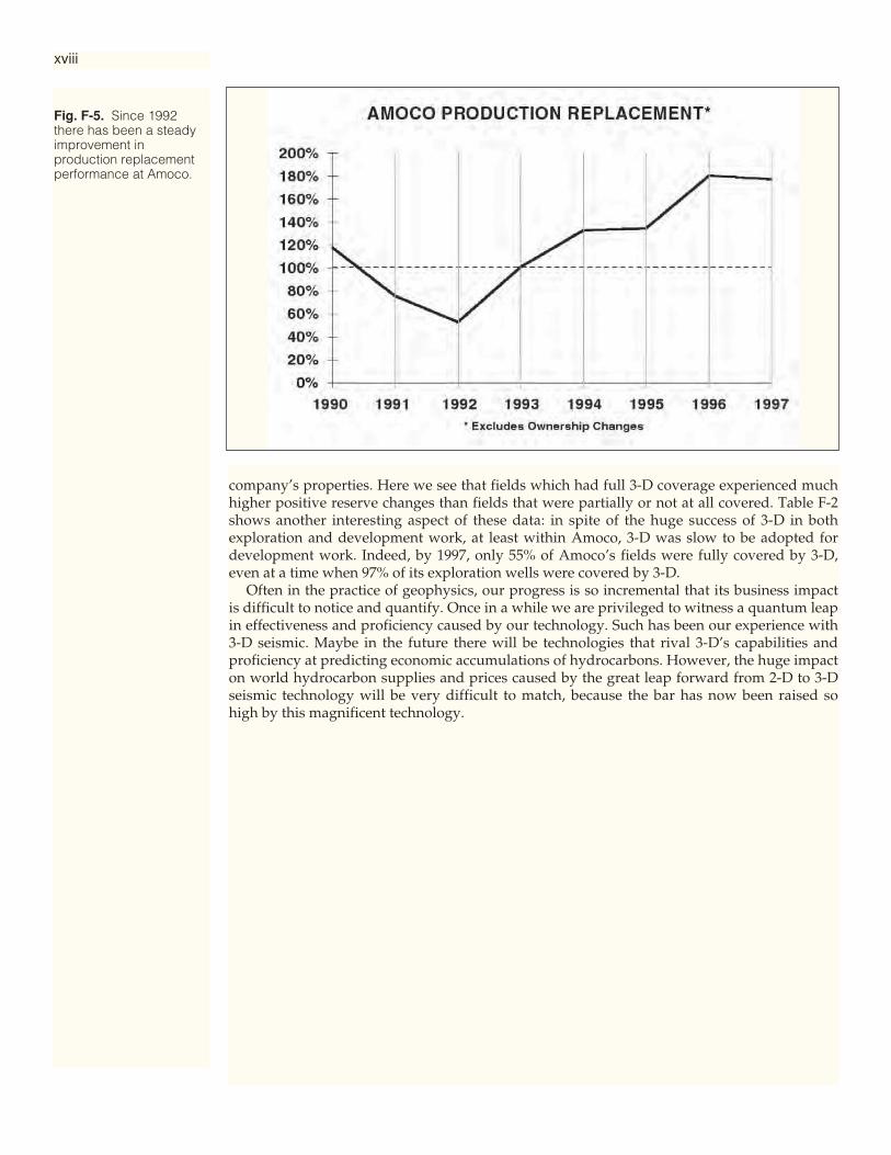
2-D seismic world to a 3-D one, and the impact amazes me even today. As can be seen, thecompany went from a 14% drilled success rate in 1990 to 47% in 1997, 5% of prospects coveredby 3-D in 1990 to 97% in 1997, a drilled success for oil wells during 1990-1997 of 3% without 3-D vs. 37% with 3-D, and a drilled success for gas wells during 1990-1997 of 24% without 3-Dvs. 54% with 3-D. Because of this success in this period, there have been major improvementsin the cost of finding and in volumes found, as is shown in Figure F-4. Here we can see thatthe cost of finding has dropped from around $8 per barrel to under $1 per barrel, while vol-umes found in 1994 and 1996 were about 1 billion BOE per year. This in turn has very benefi-cially impacted Amoco’s production replacement profile as is shown in Figure F-5.

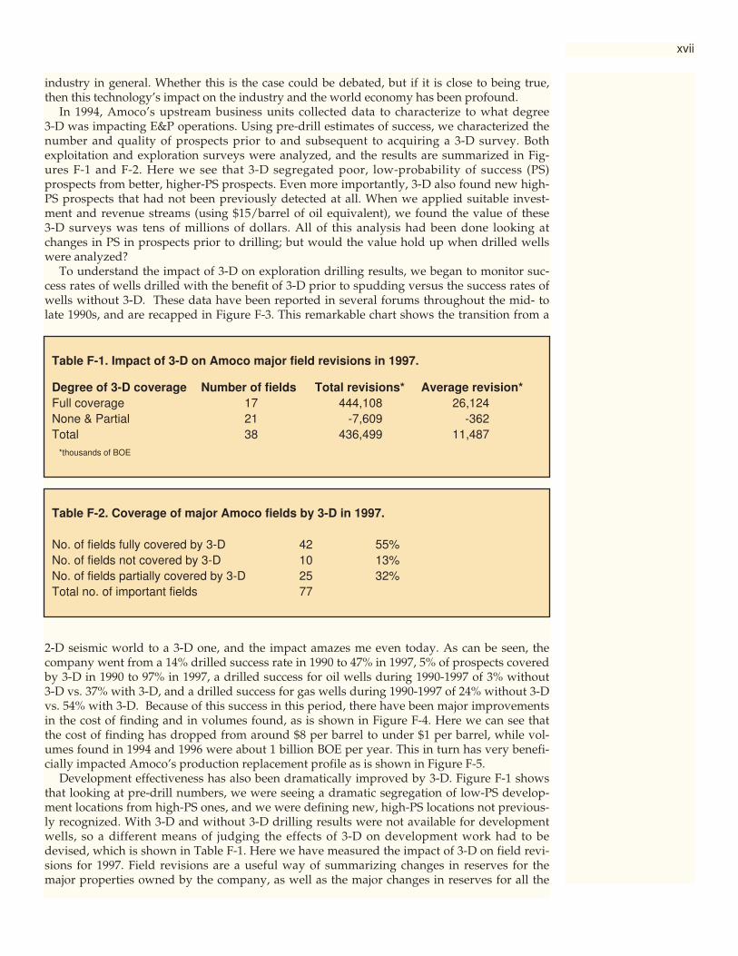
Development effectiveness has also been dramatically improved by 3-D. Figure F-1 showsthat looking at pre-drill numbers, we were seeing a dramatic segregation of low-PS develop-ment locations from high-PS ones, and we were defining new, high-PS locations not previous-ly recognized. With 3-D and without 3-D drilling results were not available for developmentwells, so a different means of judging the effects of 3-D on development work had to bedevised, which is shown in Table F-1. Here we have measured the impact of 3-D on field revi-sions for 1997. Field revisions are a useful way of summarizing changes in reserves for themajor properties owned by the company, as well as the major changes in reserves for all the

xvii

Table F-1. Impact of 3-D on Amoco major field revisions in 1997.

Degree of 3-D coverage Number of fields Total revisions* Average revision*Full coverage 17 444,108 26,124None & Partial 21 -7,609 -362 Total 38 436,499 11,487

*thousands of BOE

Table F-2. Coverage of major Amoco fields by 3-D in 1997.

No. of fields fully covered by 3-D 42 55%No. of fields not covered by 3-D 10 13%No. of fields partially covered by 3-D 25 32%Total no. of important fields 77

xviii

company’s properties. Here we see that fields which had full 3-D coverage experienced muchhigher positive reserve changes than fields that were partially or not at all covered. Table F-2shows another interesting aspect of these data: in spite of the huge success of 3-D in bothexploration and development work, at least within Amoco, 3-D was slow to be adopted fordevelopment work. Indeed, by 1997, only 55% of Amoco’s fields were fully covered by 3-D,even at a time when 97% of its exploration wells were covered by 3-D.

Often in the practice of geophysics, our progress is so incremental that its business impactis difficult to notice and quantify. Once in a while we are privileged to witness a quantum leapin effectiveness and proficiency caused by our technology. Such has been our experience with3-D seismic. Maybe in the future there will be technologies that rival 3-D’s capabilities andproficiency at predicting economic accumulations of hydrocarbons. However, the huge impacton world hydrocarbon supplies and prices caused by the great leap forward from 2-D to 3-Dseismic technology will be very difficult to match, because the bar has now been raised sohigh by this magnificent technology.

Fig. F-5. Since 1992there has been a steadyimprovement inproduction replacementperformance at Amoco.

IntroductionThe earth has always been three-dimensional and the petroleum reserves we seek

to find or evaluate are contained in three-dimensional traps. The seismic method,however, in its attempt to image the subsurface has traditionally taken a two-dimen-sional approach. It was 1970 when Walton (1972) presented the concept of three-dimensional seismic surveys. In 1975, 3-D surveys were first performed on a normalcontractual basis, and the following year Bone, Giles and Tegland (1976) presentedthe new technology to the world.

The essence of the 3-D method is areal data collection followed by the processingand interpretation of a closely-spaced data volume. Because a more detailed under-standing of the subsurface emerges, 3-D surveys have been able to contribute signifi-cantly to the problems of field appraisal, development and production as well as toexploration. It is in these post-discovery phases that many of the successes of 3-Dseismic surveys have been achieved. The scope of 3-D seismic for field developmentwas first reported by Tegland (1977).

In the late 1980s and early 1990s, the use of 3-D seismic surveys for explorationincreased significantly. This started in the mid-1980s with widely-spaced 3-D surveyscalled, for example, Exploration 3-D. Today, speculative 3-D surveys, properly sam-pled and covering huge areas, are available for purchase piecemeal in mature areaslike the Gulf of Mexico. This, however, is not the only use for exploration. Many com-panies are acquiring 3-D surveys over prospects routinely, so that the vast majority oftheir seismic budgets are for 3-D operations. The evolution and present state-of-the-art of the 3-D seismic method have recently been chronicled in a reprint volume byGraebner, Hardage, and Schneider (2001).

In the first 20 years of 3-D survey experience (1975-95) many successes and benefitswere recorded. Five particular accolades are reproduced here; others are found in thecase histories of Chapter 9 and implied at many other places throughout this book.There is a major symbiosis between modern 3-D seismic data and the interactiveworkstation.

“…there seems to be unanimous agreement that 3-D surveys result in clearer and moreaccurate pictures of geological detail and that their costs are more than repaid by the elimi-nation of unnecessary development holes and by the increase in recoverable reservesthrough the discovery of isolated reservoir pools which otherwise might be missed.”(Sheriff and Geldart, 1983)

“The leverage seems excellent for 3-D seismic to pay for itself many times over in terms ofreducing the eventual number of development wells.”(West, 1979)

History andBasic Ideas

CHAPTER ONE 1

“…the 3-D data are of significantly higher quality than the 2-D data. Furthermore, theextremely dense grid of lines makes it possible to develop a more accurate and completestructural and stratigraphic interpretation…Based on this 3-D interpretation, four success-ful oil wells have been drilled. These are located in parts of the field that could not previous-ly be mapped accurately on the basis of the 2-D seismic data because of their poor quality.This eastward extension has increased the estimate of reserves such that it was possible todeclare the field commercial in late 1980.”(Saeland and Simpson, 1982)

“…3-D seismic surveying helped define wildcat locations, helped prove additional outpostlocations, and assisted in defining untested fault blocks. Three-D seismic data helped findadditional reserves and, most certainly, provided data for more effective reservoir drainagewhile being cost-effective…Gulf participated in 16 surveys that covered 26 blocks and hasinvested $15,000,000 in these data. The results show that a 3-D seismic program can becost-effective since it can improve the success ratio of development drilling and can encour-age acceleration of a development program, thereby improving the cash flow.”(Horvath, 1985)

“We acquired two offshore blocks which contained a total of seven competitor dry holes.Our exploration department drilled one more dry hole before making a discovery. At thatpoint we conducted a 3-D survey while the platform was being prepared. When drillingcommenced, guided by the 3-D data, we had 27 successful wells out of the next 28 drilled.In this erratic depositional environment, we believe that such an accomplishment would nothave been possible without the 3-D seismic data.”(R. M. Wright, Chevron U.S.A. Inc., personal communication, May, 1988)

Sheriff (1992) addresses many benefits of 3-D seismic in Reservoir Geophysics; a fewquotations from that volume follow:

3-D seismic is an extremely powerful delineation tool, and spectacularly cost-effective, par-ticularly when well costs are high.

The success is directly attributable to the better structural interpretation made possible bythe 3-D survey.

The greatest impact of 3-D surveys has been the ability to match platform size, number ofwell slots, and production facilities to the more accurately determined field reserves.

2

WELLS DRILLED

VOLUMEOF OIL IN

PLACE

AREAOF3-D

76 78 80 82 84 86 88 90 92 94

Fig. 1-1. Area covered by3-D surveys, exploratorywells drilled and volumeof oil in place for theperiod 1976 to 1994 in theCampos Basin offshoreBrazil (from Martins et al,1995). (CourtesyPetrobras.)

Martins et al (1995), working in the Campos Basin offshore Brazil, have tracked theamount of 3-D survey coverage in relation to the wells drilled and the oil reservesbooked (Figure 1-1). This demonstrates very nicely that 3-D seismic is indeed replac-ing exploration wells!

The fundamental objective of the 3-D seismic method is increased resolution. Reso-lution has both vertical and horizontal aspects and Sheriff (1985) discusses the subjectqualitatively. The resolving power of seismic data is always measured in terms of the

Fig. 1-2. Factors affectinghorizontal and verticalseismic resolution.

Fig. 1-3. Wavelength,the seismic measuringrod, increasessignificantly with depthmaking resolutionpoorer.

BROAD BANDWIDTHBY MAXIMUM EFFORT

DATA COLLECTION

ATTENUATION OFNOISE IN

DATA PROCESSING

HORIZONTALMINIMUM SIZE

FRESNEL ZONESAMPLING

SEISMICMIGRATION

VERTICALMINIMUM THICKNESS

WAVELET

DECONVOLUTION

RESOLUTION

λ

FREQUENCYF

VELOCITYV

WAVELENGTH λ

DE

PT

H

=F—V

3

Resolution

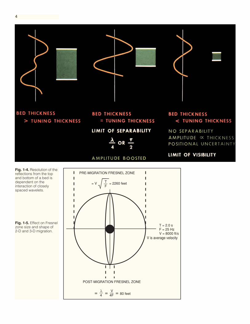
Fig. 1-4. Resolution of thereflections from the topand bottom of a bed isdependent on theinteraction of closelyspaced wavelets.

Fig. 1-5. Effect on Fresnelzone size and shape of 2-D and 3-D migration.

4

—

seismic wavelength, which is given by the quotient of velocity and frequency (Figure1-3). Seismic velocity increases with depth because the rocks are older and more com-pacted. The predominant frequency decreases with depth because the higher frequen-cies in the seismic signal are more quickly attenuated. The result is that the wave-length increases significantly with depth, making resolution poorer.

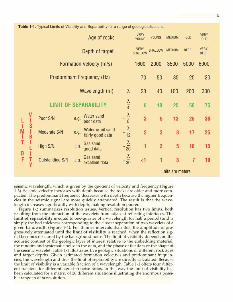
Figure 1-2 summarizes resolution issues. Vertical resolution has two limits, bothresulting from the interaction of the wavelets from adjacent reflecting interfaces. Thelimit of separability is equal to one-quarter of a wavelength (or half a period) and issimply the bed thickness corresponding to the closest separation of two wavelets of agiven bandwidth (Figure 1-4). For thinner intervals than this, the amplitude is pro-gressively attenuated until the limit of visibility is reached, when the reflection sig-nal becomes obscured by the background noise. The limit of visibility depends on theacoustic contrast of the geologic layer of interest relative to the embedding material,the random and systematic noise in the data, and the phase of the data or the shape ofthe seismic wavelet. Table 1-1 illustrates five geologic situations of different rock agesand target depths. Given estimated formation velocities and predominant frequen-cies, the wavelength and thus the limit of separability are directly calculated. Becausethe limit of visibility is a variable fraction of a wavelength, Table 1-1 offers four differ-ent fractions for different signal-to-noise ratios. In this way the limit of visibility hasbeen calculated for a matrix of 20 different situations illustrating the enormous possi-ble range in data resolution.

5

1600

70

23

6

3

2

1

<1

2000

50

40

10

5

3

2

1

3500

35

100

25

13

8

5

3

5000

25

200

50

25

17

10

7

6000

20

300

75

38

25

15

10

Formation Velocity (m/s)

Predominant Frequency (Hz)

Wavelength (m) λ

λ_4

λ_

λ_

λ_

λ_

8

12

20

30

~

~

~

~

Water sandpoor data

Water or oil sandfairly good data

Gas sandgood data

Gas sandexcellent data

Poor S/N

Moderate S/N

High S/N

Outstanding S/N

e.g.

e.g.

e.g.

e.g.

LIMIT OF SEPARABILITY

LI

MIT

OF

VISIBILITY

Depth of target

Age of rocksVERY

YOUNG YOUNG MEDIUM OLDVERYOLD

VERYSHALLOW

SHALLOW MEDIUM DEEP VERYDEEP

units are meters

Table 1-1. Typical Limits of Visibility and Separability for a range of geologic situations.

6

Migration is the principal technique for improving horizontal resolution, and indoing so performs three distinct functions. The migration process (1) repositionsreflections out-of-place because of dip, (2) focuses energy spread over a Fresnel zone,and (3) collapses diffraction patterns from points and edges. Seismic wavefronts trav-el in three dimensions and thus it is obvious that all the above are, in general, three-dimensional issues. If we treat them in two dimensions, we can only expect part ofthe potential improvement. In practice, 2-D lines are often located with strike and dipof major features in mind so that the effect of the third dimension can be minimized,but rarely eliminated. Figure 1-5 shows the focussing effect of migration in two andthree dimensions. The Fresnel zone will be reduced to an ellipse perpendicular to theline for 2-D migration (Lindsey, 1989) and to a small circle by 3-D migration. Thediameter of one-quarter of a wavelength indicated in Figure 1-5 is for perfect migra-tion. In practice, the residual Fresnel zone may be about twice this size.

The accuracy of 3-D migration depends on the velocity field, signal-to-noise ratio,migration aperture and the approach used. Assuming the errors resulting from thesefactors are small, the data will be much more interpretable both structurally andstratigraphically. Intersecting events will be separated, the confusion of diffractionpatterns will be gone, and dipping events will be moved to their correct subsurfacepositions. The collapsing of energy from diffractions and the focusing of energyspread over Fresnel zones will make amplitudes more accurate and more directlyinterpretable in terms of reservoir properties. The determination of true velocity for

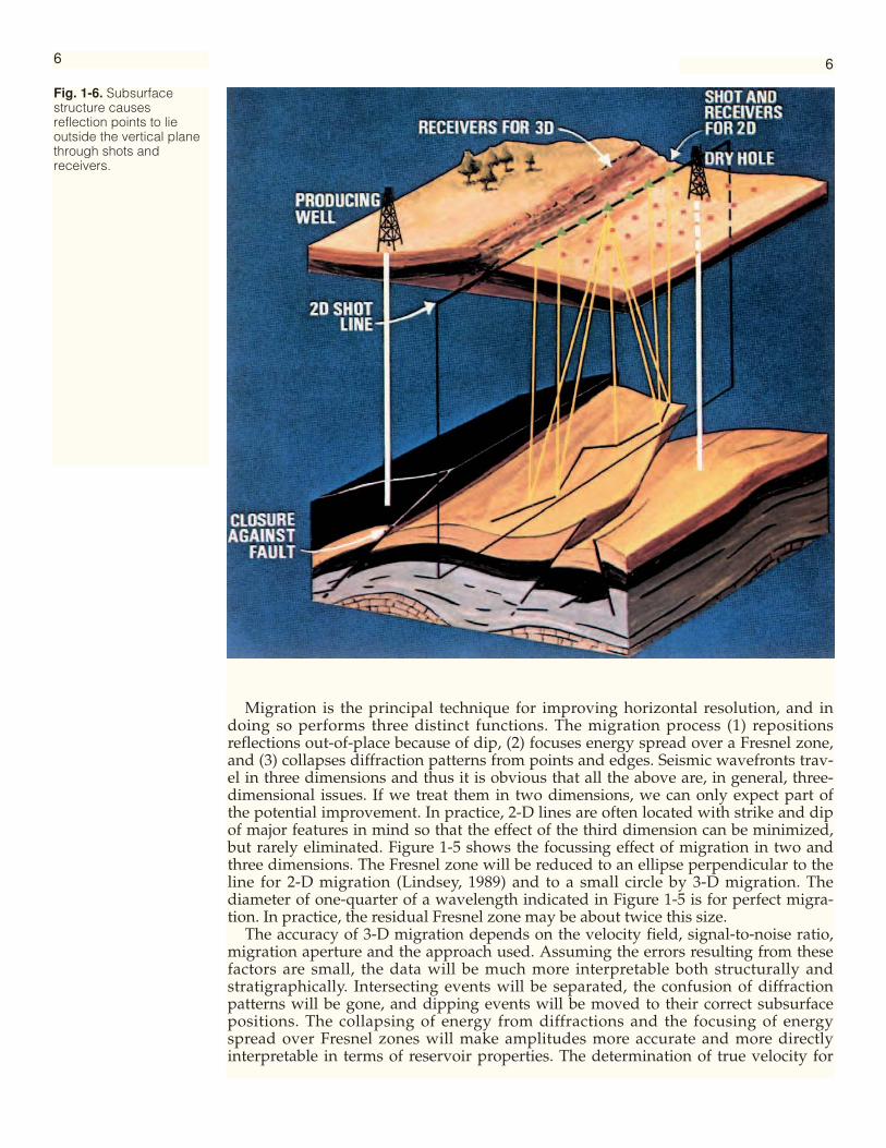
Fig. 1-6. Subsurfacestructure causesreflection points to lieoutside the vertical planethrough shots andreceivers.

6

7

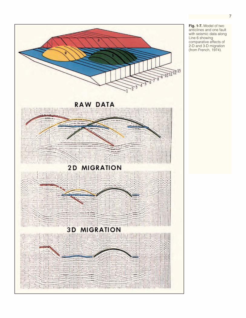
Fig. 1-7. Model of twoanticlines and one faultwith seismic data alongLine 6 showingcomparative effects of 2-D and 3-D migration(from French, 1974).

8

accurate migration and depth conversion is a significant issue. It is desirable to collectdata with a reasonable distribution of offsets and azimuths, so that the three-dimen-sional dip effects in the velocity field can be removed properly.

The interpreter of a 2-D vertical section normally assumes that the data wererecorded in one vertical plane below the line traversed by the shots and receivers. Theextent to which this is not so depends on the complexity of the structure perpendicu-lar to the line. Figure 1-6 demonstrates that, in the presence of moderate structuralcomplexity, the points at depth from which normal reflections are obtained may liealong an irregular zig-zag track. Only by migrating along and perpendicular to theline direction is it possible to resolve where these reflection points belong in the sub-surface.

French (1974) demonstrated the value of 3-D migration very clearly in modelexperiments. He collected seismic data over a model containing two anticlines and afault scarp (Figure 1-7). Thirteen lines of data were collected although only the resultsfor Line 6 are shown. The raw data have diffraction patterns for both anticlines andthe fault so the section appears very confused. The situation is greatly improved with2-D migration and anticline number 1 (shown in green) is correctly imaged, as Line 6passed over its crest. However, anticline number 2 (shown in yellow) should not

Fig. 1-8. Three-dimensionalmovement of a dippingreflection by 3-Dmigration. (CourtesyGeophysical Service Inc.)

Examples of 3-DData Improvement

9

Fig. 1-9. Improvedstructural continuity of anunconformity reflectionresulting from 2-D and 3-D migration.

occur on Line 6 and the fault scarp has the wrong slope. The 3-D migration has cor-rectly imaged the fault scarp and moved the yellow anticline away from Line 6 towhere it belongs.

Figure 1-8 demonstrates this three-dimensional event movement on real data. Thesame panel is presented before and after 3-D migration for six lines. Here we canobserve the movement of a discrete patch of reflectivity to the left and in the directionof higher line numbers.

Figure 1-9 shows improved continuity of an unconformity reflection. The 2-Dmigration has collapsed most of the diffraction patterns but some confusion remains.The crossline component of the 3-D migration removes energy not in the plane of thissection and clarifies the shape of the unconformity surface in significant detail.

10

Fig. 1-10. Improvedvisibility of a flat spotreflection after removal ofinterfering events by 3-Dmigration.

Fig. 1-11. Striking impact of3-D migration on the attitudeand continuity of reflectionsin South Australia. (CourtesySantos Ltd.)

11

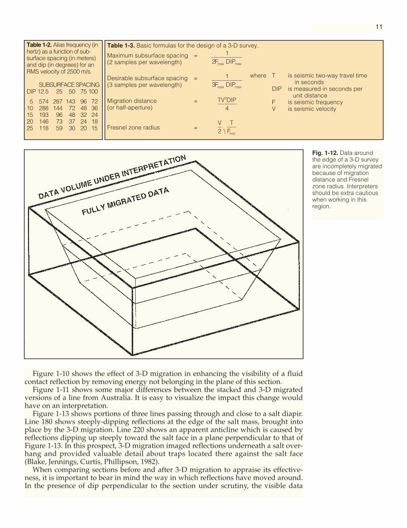
Table 1-2. Alias frequency (inhertz) as a function of sub-surface spacing (in meters)and dip (in degrees) for anRMS velocity of 2500 m/s.

SUBSURFACE SPACINGDIP 12.5 25 50 75 100

5 574 287 143 96 7210 288 144 72 48 3615 193 96 48 32 2420 146 73 37 24 1825 118 59 30 20 15

Maximum subsurface spacing =(2 samples per wavelength)

Desirable subsurface spacing =(3 samples per wavelength)

Migration distance =(or half-aperture)

Fresnel zone radius =

where T is seismic two-way travel timein seconds

DIP is measured in seconds per unit distance

F is seismic frequencyV is seismic velocity

12

13

4

2

2

F DIP

F DIP

TV DIP

V TF

max max

max max

min

Fig. 1-12. Data aroundthe edge of a 3-D surveyare incompletely migratedbecause of migrationdistance and Fresnelzone radius. Interpretersshould be extra cautiouswhen working in thisregion.

Figure 1-10 shows the effect of 3-D migration in enhancing the visibility of a fluidcontact reflection by removing energy not belonging in the plane of this section.

Figure 1-11 shows some major differences between the stacked and 3-D migratedversions of a line from Australia. It is easy to visualize the impact this change wouldhave on an interpretation.

Figure 1-13 shows portions of three lines passing through and close to a salt diapir.Line 180 shows steeply-dipping reflections at the edge of the salt mass, brought intoplace by the 3-D migration. Line 220 shows an apparent anticline which is caused byreflections dipping up steeply toward the salt face in a plane perpendicular to that ofFigure 1-13. In this prospect, 3-D migration imaged reflections underneath a salt over-hang and provided valuable detail about traps located there against the salt face(Blake, Jennings, Curtis, Phillipson, 1982).

When comparing sections before and after 3-D migration to appraise its effective-ness, it is important to bear in mind the way in which reflections have moved around.In the presence of dip perpendicular to the section under scrutiny, the visible data

Table 1-3. Basic formulas for the design of a 3-D survey.

12

Fig

. 1-1

3.Th

ree

vert

ical

sec

tions

thro

ugh

or a

dja

cent

to a

Gul

f of

Mex

ico

salt

dom

e b

efor

e m

igra

tion

(top

) an

d a

fter

mig

ratio

n (b

otto

m),

show

ing

the

rep

ositi

onin

g o

f sev

eral

ref

lect

ions

nea

r th

e sa

lt fa

ce.

(Cou

rtes

y H

unt O

il C

omp

any.

)

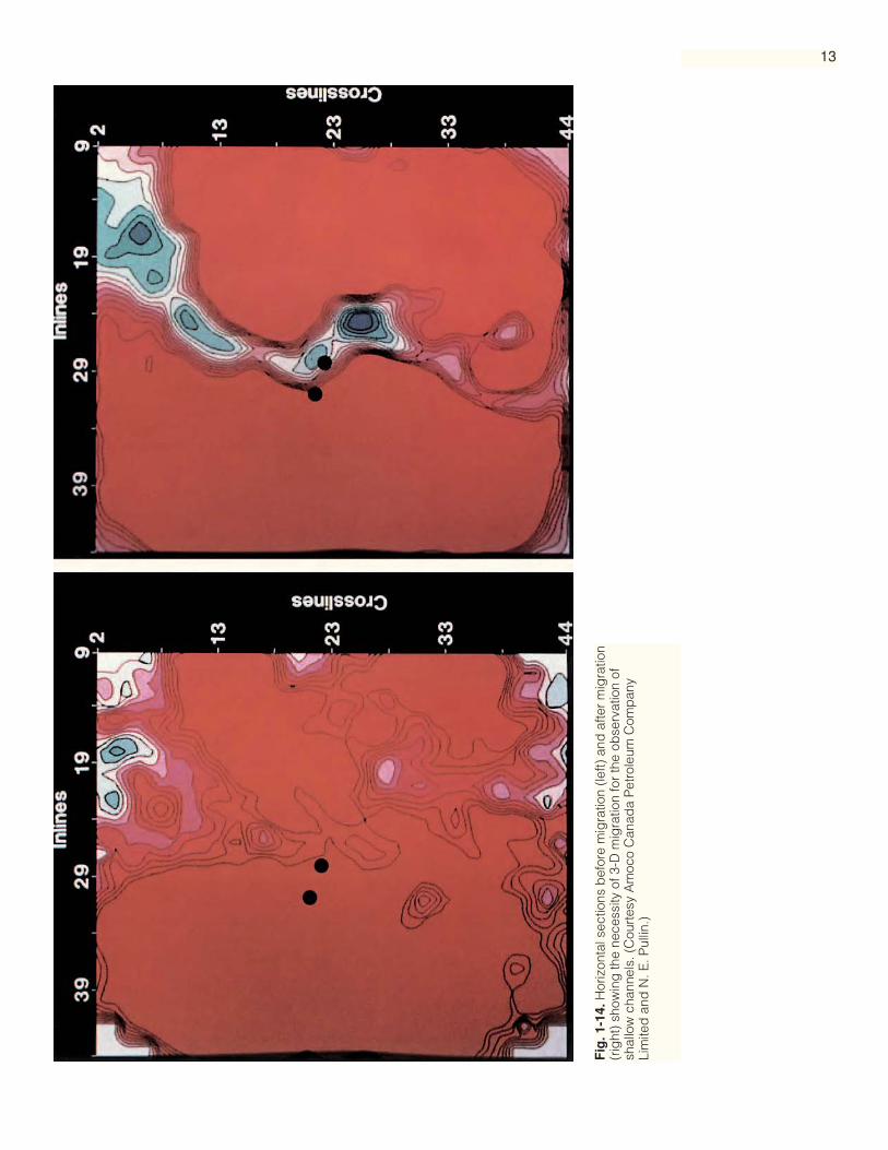
Fig

. 1-1

4. H

oriz

onta

l sec

tions

bef

ore

mig

ratio

n (le

ft) a

nd a

fter

mig

ratio

n(r

ight

) sh

owin

g th

e ne

cess

ity o

f 3-D

mig

ratio

n fo

r th

e ob

serv

atio

n of

shal

low

cha

nnel

s. (

Cou

rtes

y A

moc

o C

anad

a P

etro

leum

Com

pan

yLi

mite

d a

nd N

. E. P

ullin

.)

13

14

before and after 3-D migration are different. It is unreasonable to compare detailedcharacter and deduce what 3-D migration did. It is possible to compare a sectionbefore 3-D migration with the one from the same location after 3-D migration andfind that a good quality reflection has disappeared. The migrated section is not conse-quently worse; the good reflection has simply moved to its correct location in the sub-surface.

Figure 1-14 shows a horizontal section at a time of 224 ms from a very high resolu-tion 3-D survey in Canada aimed at monitoring a steam injection process. The sectionon the left is from the 3-D volume before migration and the section on the right isfrom the volume after migration. The two black dots indicate wells. The striking visi-bility of a channel after migration results from the focusing of energy previouslyspread over the Fresnel zone. The fact that one well penetrates the channel and theother does not is significant: they are only 10 m apart.

The sampling theorem requires that, for preservation of information, a waveformmust be sampled such that there are at least two samples per cycle for the highest fre-quency. Since the beginning of the digital era, we have been used to sampling a seis-mic trace in time. For example, 4 ms sampling is theoretically adequate for frequen-cies up to 125 Hz. In practice we normally require at least three samples per cycle forthe highest frequency. With this safety margin, 4 ms sampling is adequate for frequen-cies up to 83 Hz.

In space, the sampling theorem translates to the requirement of at least two, andpreferably three, samples per shortest wavelength in every direction. In a normal 2-Dsurvey layout this will be satisfied by the depth point spacing along lines but not bythe spacing between lines. Hence the restriction that widely-spaced 2-D lines can beprocessed individually on a 2-D basis but not together as a 3-D volume.

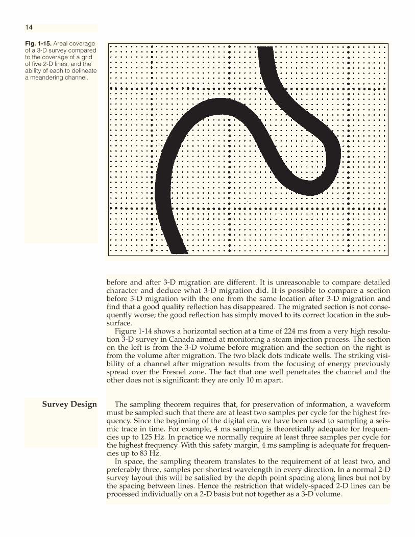
Fig. 1-15. Areal coverageof a 3-D survey comparedto the coverage of a gridof five 2-D lines, and theability of each to delineatea meandering channel.

Survey Design

If the sampling theorem is not satisfied the data are aliased. In the case of a dippingevent, the spatial sampling of that event must be such that its principal alignment isobvious; if not, aliases occur and spurious dips result after multichannel processing.Table 1-2 shows the frequencies at which this aliasing occurs for various dips and sub-surface spacings. Clearly, a 3-D survey must be designed such that aliasing during pro-cessing does not occur. Tables like the one presented can be used to establish the neces-sary spacing considering the dips and velocities present. In order to impose the safetymargin of three samples, rather than two, per shortest wavelength, the frequency limitis normally considered to be around two-thirds of each number tabulated. The formu-las in Table 1-3 provide a general method of establishing the spacings required. The

Fig. 1-16. 3-D datavolume showing a Gulf ofMexico salt dome andassociated rim syncline.(Courtesy Hunt OilCompany).

15

16

first formula, based on two samples per shortest wavelength, gives the maximumspacing that can be used to image the structure. Given our ignorance of the subsurfacestructure at the time the 3-D survey is being designed, we should allow a significantsafety margin by collecting at least three samples per shortest spatial wavelength.

Table 1-3 also shows the two formulas needed to calculate the width of the extrastrip around the periphery of the prospect over which data must be collected in orderto ensure proper imaging in the area of interest. The calculation of migration distance,the extra fringe width needed for structure, should use the local value of dip mea-sured perpendicular to the prospect boundary. The Fresnel zone radius, the extrafringe width needed for stratigraphy, needs to be considered for the proper focusingof amplitudes. The two strip, or fringe, widths thus calculated should be addedtogether in defining the total survey area.

A typical 3-D seismic interpreter does not get involved in designing surveys butnevertheless needs to appreciate these issues. Figure 1-12 demonstrates that, of thedata volume under interpretation, only the central portion is fully migrated andtherefore fully reliable. The fringe between the inner and outer volumes is the migra-tion distance and the Fresnel zone radius. If the interpreter is working in this fringezone he needs to realize that the data are unreliable and the results are subject togreater risk.

Proper design of a 3-D survey is critical to its success, and sufficiently close spacingis vital. The formulas of Table 1-3 are addressing structural design issues. In areas of

Fig. 1-17. 3-D datavolume showing a brightspot from a Gulf ofMexico gas reservoir.(Courtesy Chevron U.S.A.Inc.)

17

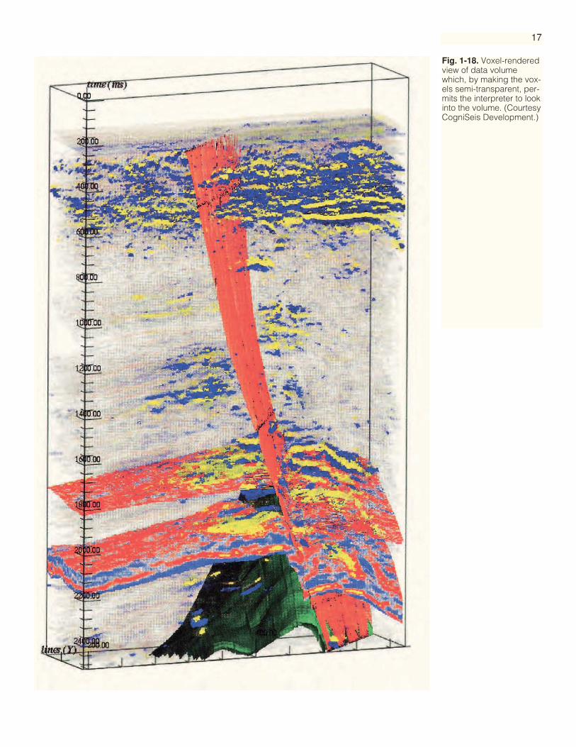
Fig. 1-18. Voxel-renderedview of data volumewhich, by making the vox-els semi-transparent, per-mits the interpreter to lookinto the volume. (CourtesyCogniSeis Development.)

18

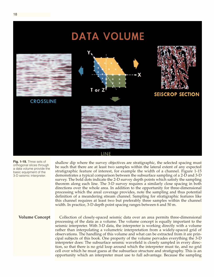
Fig. 1-19. Three sets oforthogonal slices througha data volume provide thebasic equipment of the 3-D seismic interpreter.

shallow dip where the survey objectives are stratigraphic, the selected spacing mustbe such that there are at least two samples within the lateral extent of any expectedstratigraphic feature of interest, for example the width of a channel. Figure 1-15demonstrates a typical comparison between the subsurface sampling of a 2-D and 3-Dsurvey. The bold dots indicate the 2-D survey depth points which satisfy the samplingtheorem along each line. The 3-D survey requires a similarly close spacing in bothdirections over the whole area. In addition to the opportunity for three-dimensionalprocessing which the areal coverage provides, note the sampling and thus potentialdefinition of a meandering stream channel. Sampling for stratigraphic features likethis channel requires at least two but preferably three samples within the channelwidth. In practice, 3-D depth point spacing ranges between 6 and 50 m.

Collection of closely-spaced seismic data over an area permits three-dimensionalprocessing of the data as a volume. The volume concept is equally important to theseismic interpreter. With 3-D data, the interpreter is working directly with a volumerather than interpolating a volumetric interpretation from a widely-spaced grid ofobservations. The handling of this volume and what can be extracted from it are prin-cipal subjects of this book. One property of the volume pervades everything the 3-Dinterpreter does: The subsurface seismic wavefield is closely sampled in every direc-tion, so that there is no grid loop around which the interpreter must tie, and no gridcell over which he must guess at the subsurface structure and stratigraphy. This is anopportunity which an interpreter must use to full advantage. Because the sampling

Volume Concept

19

requirements for interpretation are the same as for processing, all the processed datapoints contain unique information and thus should be used in the interpretation.Thus, the interpreter of a 3-D volume should not decimate the data available to himbut, given that he has time constraints imposed on him, he should use innovativeapproaches with horizontal sections, specially selected slices, and automatic spatialtracking, in order to comprehend all the information in the data. In this way the 3-Dseismic interpreter will generate a more accurate and detailed map or other productthan his 2-D predecessor in the same area.

Figure 1-16 shows a view of a 3-D data volume through a salt dome. It demon-strates the volume concept well and the interpreter can use a display of this kind tohelp in appreciation of subsurface three-dimensionality. Figure 1-17 shows anothercube, in this case generated interactively, which helps in the three-dimensional appre-ciation of a much more detailed subsurface objective. Neither of these displays, how-ever, permits the interpreter to look into the volume of data.

True 3-D display has recently become a reality on computer workstations and Fig-ure 1-18 shows an example. The portion of the volume being displayed is composedof voxels, or volume elements, and these are rendered with differing degrees of trans-parency so that the interpreter can really see into the volume. In Figure 1-18 there arefour interpreted surfaces as well as the semi-transparent data. As with any volumetricdisplay the dynamic range is reduced because of the quantity of data viewed. Thesetypes of display are very useful for data visualization but they are not yet fully inte-grated into mainstream interpretation systems.

The vast majority of 3-D interpretation is performed on slices through the data vol-ume. There are no restrictions on the dynamic range for the display of any one slice,and therefore all the benefits of color, dual polarity, etc., can be exploited (see Chapter2). The 3-D volume contains a regularly-spaced orthogonal array of data pointsdefined by the acquisition geometry and maybe adjusted during processing. Thethree principal directions of the array define three sets of orthogonal slices or sectionsthrough the data, as shown in Figure 1-19.

The vertical section in the direction of boat movement or cable lay-out is called aline (sometimes an inline). The vertical section perpendicular to this is called a

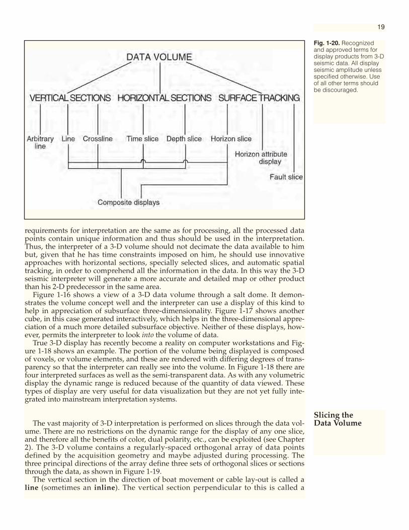
Fig. 1-20. Recognizedand approved terms fordisplay products from 3-Dseismic data. All displayseismic amplitude unlessspecified otherwise. Useof all other terms shouldbe discouraged.

Slicing theData Volume

20

crossline. The horizontal slice is called a horizontal section, time slice, Seiscrop* sec-tion, or depth slice. The terminology used for slices through 3-D data volumes hasbecome somewhat confused. One of the objectives of this chapter is to clarify terms incommon use today.

Three sets of orthogonal slices through the data volume (as defined above) areregarded as the basic equipment of the 3-D interpreter. A complete interpretation willmake use of some of each of them. However, many other slices through the volumeare possible. A diagonal line may be extracted to tie two locations of interest, such aswells. A zig-zag sequence of diagonal line segments may be necessary to tie togetherseveral wells in a prospect. In the planning stages for a production platform, a diago-nal line may be extracted through the platform location along the intended azimuthof a deviated well. All these are vertical sections and are referred to as arbitrary lines.

More complicated slices are possible for special applications. A slice along or paral-lel to a structurally interpreted horizon, and hence along one bedding plane, is a hori-zon slice, horizon Seiscrop section, or amplitude map. Slices of this kind have par-ticular application for stratigraphic interpretation, which is explored in Chapter 4.Fault slices generated parallel to a fault face have various applications in structuraland reservoir interpretation and will be discussed in Chapter 7. Horizon attributedisplays are the subject of Chapter 8.

*Trademark of Geophysical Service Inc.

Fig. 1-21. An early opticalworkstation.

21

Figure 1-20 shows a hierarchy of approved terms for display products from 3-Dseismic data. It shows, for example, the equivalence of horizontal and vertical sec-tions, and the equivalence of time slices with lines and crosslines. In order to aidworldwide communication, use of other terms is discouraged.

Because 3-D interpretation is performed with data slices and because there is a verylarge number of slices for a typical data volume, several innovative approaches formanipulating the data have emerged. In the early days of 3-D development asequence of horizontal sections was displayed on film-strip and shown as a motionpicture (Bone, Giles, Tegland, 1983). From this developed the Seiscrop InterpretationTable — initially a commercially-available piece of equipment incorporating a 16mmanalytical movie projector. This machine was originally developed for coaches want-ing to examine closely the actions of professional athletes.

The Seiscrop Interpretation Table then evolved into a custom-built device (Figure 1-21). The data, either horizontal or vertical sections, were projected from 35mm film-strip onto a large screen. The interpreter fixed a sheet of transparent paper over thescreen for mapping and then adjusted the size of the data image, focus, frameadvance, or movie speed by simple controls.

Today 3-D interpretation is performed interactively and there has been an explo-sion in workstation usage in recent years. The interpreter calls the data from diskand views them on the screen of a color monitor (Figure 1-22). The large amount ofregularly-organized data in a 3-D volume gives the interactive approach enormous

Fig. 1-22. An earlyinteractive workstation.

Manipulatingthe Slices

benefits. In fact, many interactive interpretation systems addressed 3-D data first asthe easier problem, and then developed 2-D interpretation capabilities later.

Most of the interpretation discussed in this book resulted from use of an interactiveworkstation, and many of the data illustrations are actual screen photographs. Fur-thermore, the facilities of the system contributed in several significant ways to thesuccess of many of the projects reported here. Hence it is appropriate to review theinterpretive benefits of an interactive interpretation system.

(1) Data management — The interpreter needs little or no paper; the selected seis-mic data display is presented on the screen of a color monitor and the progressiveresults of interpretation are returned to the digital database.

(2) Color — Flexible color display provides the interpreter with maximum opticaldynamic range adapted to the particular problem under study.

(3) Image composition — Data images can be composed on the screen so that theinterpreter views what is needed, no more and no less, for the study of one particularissue. Slices through the data volume are designed by the user in order to customizethe perspective to the problem.

(4) Idea flow — The rapid response of the system makes it easy to try new ideas.The interpreter can rapidly generate innovative map or section products in pursuit ofa better interpretation.

(5) Interpretation consistency — The capability to review large quantities of datain different forms means that the resulting interpretation should be more consistentwith all available evidence. This is normally considered the best measure of interpre-tation quality.

(6) More information — Traditional interpretive tasks performed interactively willsave time; however, the extraction of more detailed subsurface information is morepersuasive and far-reaching.

Interactive interpretation must commence with data loading and this is a criticalfirst step. Should the data be loaded at 8, 16 or 32 bits? Is clipping of the highestamplitudes acceptable?

Data processing has always been performed using 32 bits to describe each ampli-tude value. This large word size ensures that significance is retained during all com-putations. The first interactive systems in the early 1980's were 32-bit machines butsoon a demand for speed dictated that data be loaded using 8 bits only. The smallword reduces response time and minimizes storage space for the survey data. Todayinteractive systems offer a choice of 8-bit, 16-bit or 32-bit dynamic range althoughcolor monitors normally display 8 bits only.

Figure 1-23 shows a typical statistical distribution of amplitudes in a data volume.There are a large number of very low amplitudes, a fairly large number of moderateamplitudes but a very small number of high amplitudes. Mainstream structural inter-pretation tends to work on moderate amplitude horizons. The high amplitude tails ofthe distribution are localized anomalies which, in tertiary clastic basins, are often thehydrocarbon bright spots. The interpreter avoids the low amplitudes as much as pos-sible because they are the most subject to noise. Thus most interpretive time is devot-ed to the amplitudes lying in the stippled areas of Figure 1-23.

If interpretation is to be conducted using 8-bits only, scaling 32-bit amplitude num-bers to 8-bit amplitude numbers must be done during data loading. If the maximumamplitude in the volume is set to ± 128, relative amplitudes are preserved within theprecision of the 8 bits. However, this often severely limits the dynamic range availablein the stippled, or heavily used, amplitude regions. Clipping of the highest ampli-tudes is a common reaction to this problem so that a smaller value is set to ±128. Moredynamic range is then available for the mainstream structural interpretation but thehighest amplitudes are destroyed and hence unavailable for stratigraphic or reservoiranalysis. This can be very damaging particularly in areas like the Gulf of Mexico.Some interactive workstations load 8-bit data with a floating point scalar defined

22

Dynamic Rangeand Data Loading

23

Fig. 1-24. Test for anddemonstration of dataclipping.

NUMBERS OF SAMPLESIN DATA VOLUME

Most interpretive time

Clipped

-128 -128 0 +128 +128

AMPLITUDE

Fig. 1-23. Typicalstatistical distribution ofamplitudes in a 3-D datavolume. Plus or minus128, the largest numberwhich can be describedby 8 bits, may be set tothe largest amplitude, oralternatively to somesmaller amplitude, thuscausing data clipping.

individually for each trace and stored in the trace header. This lessens but does notremove the dynamic range problem discussed above.

A common and generally desirable solution today is to load the data using 16 bitsfor each amplitude value. In this way clipping is irrelevant and unnecessary as thereis plenty of dynamic range for structural interpretation and bright spot studies.

An interesting comparison of 8-bit and 16-bit interpretation was conducted byRoberts and Hughes (1995). They concluded that there are always differencesbetween interpretation products from 8-bit and 16-bit volumes but they are generallyless than 5%. These are often tolerable but they stressed the need for sensible clipping.Figure 1-24 is a test for and demonstration of data clipping. Contrasting colors havebeen placed in the extremities of the otherwise-gradational color scheme. The largeamounts of yellow and cyan demonstrate an anomalously high occupancy of thosehighest amplitudes, that is the data has been heavily clipped.

The author is opposed to data clipping as it places restrictions on interpretationactivities. Generally the best solution is to use 16 bits and sometimes 32 bits. The totalinterpretation project today often involves a significant amount of post-interpretationcomputation. The larger number of bits helps ensure that numeric significance ismaintained during these operations. Fortunately faster and cheaper hardware is nowavailable which makes the use of 16 or 32 bits much less of a burden than it was in thepast.

Seismic technology has, over the years, become increasingly complex. Whereas aparty chief used to handle data collection, processing, and interpretation, experts arenow generally restricted to each discipline. Data processing involves many highlysophisticated operations and is conducted in domains unfamiliar to the nonmathe-matically-minded interpreter. The ability of certain processes to transform data inadverse as well as beneficial ways is striking.

Today’s seismic interpreter must understand in some detail what has been done tothe data and must understand data processing well enough to ask meaningful ques-tions of the processing staff. A summary of 3-D data collection and processing issuesis included as Appendix A. Today’s interpreter will also benefit greatly by using hightechnology aids, such as an interactive system. Critical to maximum effectiveness isan understanding of the advantages of color and how to work with horizontal sec-tions, acoustic impedance sections, frequency sections, vertical seismic profiles,attribute displays, and the like.

Seismic interpretation today thus involves a wide range of seismic technologies. Ifthe results of these are studied by the interpreter in concert, significant synergism canresult. However, pragmatism retains its place. The interpreter must continue to take abroad view, to integrate geology and geophysics, and, to an increasing degree, engi-neering, and to make simplifying assumptions in order to get the job done. Theprogress of seismic interpretation depends on the continued coexistence of technolog-ical synergism and creative pragmatism.

Blake, B. A., J. B. Jennings, M. P. Curtis, and R. M. Phillipson, 1982, Three-dimensionalseismic data reveals the finer structural details of a piercement salt dome: OffshoreTechnology Conference paper 4258, p. 403-406.

Bone, M. R., B. F. Giles, and E. R. Tegland, 1976, 3-D high resolution data collection,processing and display: Houston, Texas, presented at 46th Annual SEG Meeting.

Bone, M. R., B. F. Giles, and E. R. Tegland, 1983, Analysis of seismic data using hori-zontal cross-sections: Geophysics, v. 48, p. 1172-1178.

French, W. S., 1974, Two-dimensional and three-dimensional migration of model-experiment reflection profiles: Geophysics, v. 39, p. 265-277.

Graebner, R. J., B. A. Hardage, and W. A. Schneider, 2001, 3-D seismic exploration:SEG Geophysics Reprint Series, no. 22, 857 p.

24

References

Synergism andPragmatism inInterpretation

25

Horvath, P. S., 1985, The effectiveness of offshore three-dimensional seismic surveys— case histories: Geophysics, v. 50, p. 2411-2430.

Lindsey, J. P., 1989, The Fresnel zone and its interpretive significance: The LeadingEdge, v. 8, no. 10, p. 33-39.

Martins, C. C., and C. A. da Costa, C. E Theodoro, L. R. Guardado, and V. F. Andrade,1995, 3-D Seismic: A successful strategy in the Campos Basin: The Leading Edge, v.14, p. 701–704.

Roberts, G. A., and M. J. Hughes, 1995, Workstation interpretation — a comparison ofdata stored at 8 and 16 bits: Poster paper and EAGE Annual Convention, Glasgow.

Saeland, G. T., and G. S. Simpson, 1982, Interpretation of 3-D data in delineating asub-unconformity trap in Block 34/10, Norwegian North Sea, in M. T. Halbouty,ed., The deliberate search for the subtle trap: AAPG Memoir 32, p. 217-236.

Sheriff, R. E., 1985, Aspects of seismic resolution, in O. R. Berg and D. Woolverton,eds., Seismic stratigraphy II: an integrated approach to hydrocarbon exploration:AAPG Memoir 39, p. 1-10.

Sheriff, R. E. (editor), 1992, Reservoir Geophysics, SEG Investigations in Geophysicsno. 7.

Sheriff, R. E. and L. P. Geldart, 1983, Exploration seismology; v. 2, data-processing andinterpretation: Cambridge University Press, p. 130.

Tegland, E. R., 1977, 3-D seismic techniques boost field development: Oil and GasJournal, v. 75, no. 37, p. 79-82.

Walton, G. G., 1972, Three-dimensional seismic method: Geophysics, v. 37, p. 417-430.West, J., 1979, Development near for Thailand field: Oil and Gas Journal, v. 77, no. 32,

p. 74-76.

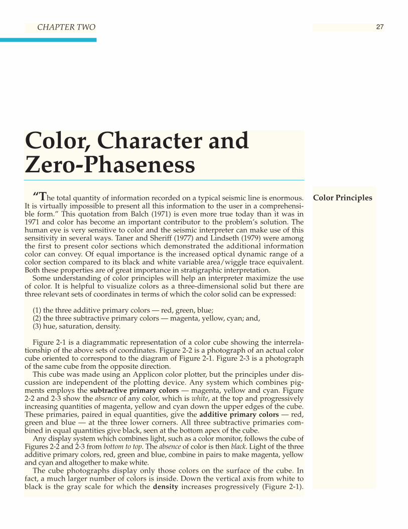
27

Color, Character andZero-Phaseness

“The total quantity of information recorded on a typical seismic line is enormous.It is virtually impossible to present all this information to the user in a comprehensi-ble form.” This quotation from Balch (1971) is even more true today than it was in1971 and color has become an important contributor to the problem’s solution. Thehuman eye is very sensitive to color and the seismic interpreter can make use of thissensitivity in several ways. Taner and Sheriff (1977) and Lindseth (1979) were amongthe first to present color sections which demonstrated the additional informationcolor can convey. Of equal importance is the increased optical dynamic range of acolor section compared to its black and white variable area/wiggle trace equivalent.Both these properties are of great importance in stratigraphic interpretation.

Some understanding of color principles will help an interpreter maximize the useof color. It is helpful to visualize colors as a three-dimensional solid but there arethree relevant sets of coordinates in terms of which the color solid can be expressed:

(1) the three additive primary colors — red, green, blue;(2) the three subtractive primary colors — magenta, yellow, cyan; and,(3) hue, saturation, density.

Figure 2-1 is a diagrammatic representation of a color cube showing the interrela-tionship of the above sets of coordinates. Figure 2-2 is a photograph of an actual colorcube oriented to correspond to the diagram of Figure 2-1. Figure 2-3 is a photographof the same cube from the opposite direction.

This cube was made using an Applicon color plotter, but the principles under dis-cussion are independent of the plotting device. Any system which combines pig-ments employs the subtractive primary colors — magenta, yellow and cyan. Figure2-2 and 2-3 show the absence of any color, which is white, at the top and progressivelyincreasing quantities of magenta, yellow and cyan down the upper edges of the cube.These primaries, paired in equal quantities, give the additive primary colors — red,green and blue — at the three lower corners. All three subtractive primaries com-bined in equal quantities give black, seen at the bottom apex of the cube.

Any display system which combines light, such as a color monitor, follows the cube ofFigures 2-2 and 2-3 from bottom to top. The absence of color is then black. Light of the threeadditive primary colors, red, green and blue, combine in pairs to make magenta, yellowand cyan and altogether to make white.

The cube photographs display only those colors on the surface of the cube. Infact, a much larger number of colors is inside. Down the vertical axis from white toblack is the gray scale for which the density increases progressively (Figure 2-1).

Color Principles

CHAPTER TWO

28

The saturation measures the distance from this central axis, ranging from zero onthe axis to 100% on the surface of the cube. The hue is the rotational parameter mea-suring the spectral content of a color.

For the color cube illustrated in Figures 2-2 and 2-3 there are 17 levels (0-16) of eachof the subtractive primaries — magenta, yellow and cyan. The total number of colorsin the cube is thus 17 × 17 × 17 or 4,913, of which 1,538 are fully saturated colors onthe surface. One way of studying the colors available inside the cube is to slice italong a chosen density level. Figure 2-4 shows density level 16, which has maximumstrength magenta, yellow and cyan at the corners and gray of density 33% at the cen-ter. This display clearly demonstrates the significance of hue as the rotational parame-ter and saturation as the radial distance from the gray axis. The additive primaries,red, green and blue, lie on density level 32 with gray of density 67% at the center.

Figure 2-5 is a color chart used in an interactive interpretation system (Gerhard-stein and Brown, 1984). It is based on the mixing of light and hence involves the addi-tive primaries — red, green and blue. All the colors displayed in Figure 2-5 are fullysaturated; that is, they lie only on the surface of the color cube. The right half of thechart is a projection of a color cube similar to that of Figures 2-2 and 2-3 when viewedfrom the top. The left half of the chart is a view of the same color cube from the bot-tom. Interactive workstations make the selection and building of logical, efficient andintuitive color schemes easier if the selection chart is founded directly on the colorcube, as in Figure 2-5.

Today’s interpreter uses color in two fundamentally different ways: with a contrast-ing or with a gradational color scheme. A map or a section displayed in contrasting col-

Fig. 2-1. Diagram of acolor cube showing therelationship of thesubtractive primary colors(magenta, yellow andcyan) to the additiveprimary colors (red, greenand blue) to the colorparameters (hue,saturation and density).

InterpretiveValue of Color

29

ors is normally accompanied by a legend, so the reader can identify the value of thedisplayed attribute at any point by reading the range of values associated with eachcolor. Figure 2-6 is a structural contour map with a contour interval of 20 ms.

For an effective color display it is important that the range of values associatedwith each color, the number of colors used and their sequence, the contrast betweenadjacent colors, and the display scales are all carefully chosen. A color display mustconvey useful information and at the same time be aesthetically pleasing. For a mapsuch as Figure 2-6 it is desirable to perceive equal visual contrast between adjacentcolors, so that no one color boundary is more outstanding than another. A spectralsequence of colors was selected.

Figure 2-7 is a nomogram used for assessing visual color contrast. Visual contrastbetween two colors is, of course, somewhat subjective. Numerical color contrast is thesum of the absolute values of the differences in the amounts of the three primary col-ors. Zero density is white, maximum density (100%) is black, and density can have

Fig. 2-2. Photograph of acolor cube oriented thesame as the diagram inFigure 2-1.

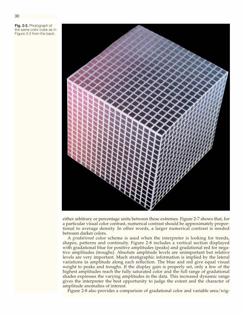
30

either arbitrary or percentage units between these extremes. Figure 2-7 shows that, fora particular visual color contrast, numerical contrast should be approximately propor-tional to average density. In other words, a larger numerical contrast is neededbetween darker colors.

A gradational color scheme is used when the interpreter is looking for trends,shapes, patterns and continuity. Figure 2-8 includes a vertical section displayedwith gradational blue for positive amplitudes (peaks) and gradational red for nega-tive amplitudes (troughs). Absolute amplitude levels are unimportant but relativelevels are very important. Much stratigraphic information is implied by the lateralvariations in amplitude along each reflection. The blue and red give equal visualweight to peaks and troughs. If the display gain is properly set, only a few of thehighest amplitudes reach the fully saturated color and the full range of gradationalshades expresses the varying amplitudes in the data. This increased dynamic rangegives the interpreter the best opportunity to judge the extent and the character ofamplitude anomalies of interest.

Figure 2-8 also provides a comparison of gradational color and variable area/wig-

Fig. 2-3. Photograph ofthe same color cube as inFigure 2-2 from the back.

31

gle trace for the same piece of data. The shortcomings in the variable area/wiggletrace display relative to the color section are: (1) the visual weights of peaks andtroughs are very different, which makes comparison difficult and biases the inter-preter’s eye towards the peaks; (2) some of the peaks are saturated or clipped; and (3)the troughs, where they have significant amplitudes, are not visible beneath the depthpoints where they belong. The red flat spot reflection is clearly visible on the colorsection as are the relative amplitudes of peaks and troughs. At the extreme right ofthe section, coincident amplitude maxima in the peak and the trough indicate a tun-ing phenomenon (see Chapter 6).

Figure 2-9 provides a similar comparison between gradational color and variablearea/wiggle trace. In addition, three different horizontal scales are used from which afurther shortcoming of variable area/wiggle trace is apparent — that the dynamicrange is limited and dependent on horizontal scale.

The color schemes of Figures 2-8 and 2-9 are more explicitly called double-grada-tional schemes with symmetry of blue and red about zero amplitude. The need forequal visibility of peaks and troughs has long been recognized. Backus and Chen

Fig. 2-4. Horizontal slicethrough the color cube atdensity level 33%,showing magenta, yellowand cyan at the cornersand gray at the center.

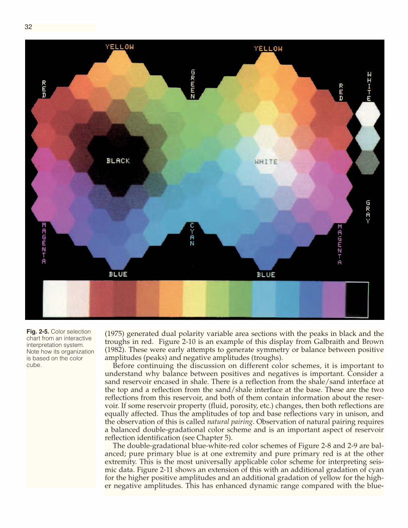
32

(1975) generated dual polarity variable area sections with the peaks in black and thetroughs in red. Figure 2-10 is an example of this display from Galbraith and Brown(1982). These were early attempts to generate symmetry or balance between positiveamplitudes (peaks) and negative amplitudes (troughs).

Before continuing the discussion on different color schemes, it is important tounderstand why balance between positives and negatives is important. Consider asand reservoir encased in shale. There is a reflection from the shale/sand interface atthe top and a reflection from the sand/shale interface at the base. These are the tworeflections from this reservoir, and both of them contain information about the reser-voir. If some reservoir property (fluid, porosity, etc.) changes, then both reflections areequally affected. Thus the amplitudes of top and base reflections vary in unison, andthe observation of this is called natural pairing. Observation of natural pairing requiresa balanced double-gradational color scheme and is an important aspect of reservoirreflection identification (see Chapter 5).

The double-gradational blue-white-red color schemes of Figure 2-8 and 2-9 are bal-anced; pure primary blue is at one extremity and pure primary red is at the otherextremity. This is the most universally applicable color scheme for interpreting seis-mic data. Figure 2-11 shows an extension of this with an additional gradation of cyanfor the higher positive amplitudes and an additional gradation of yellow for the high-er negative amplitudes. This has enhanced dynamic range compared with the blue-

Fig. 2-5. Color selectionchart from an interactiveinterpretation system.Note how its organizationis based on the colorcube.

33

white-red but still has perfect balance on the color cube. Blue and red are both addi-tive primaries, and cyan and yellow are both subtractive primaries. These balanceddouble-gradational color schemes are particularly important for reservoir reflectionidentification and recognition of hydrocarbon fluid effects.

Figure 2-12 shows a single-gradational gray scale with black at maximum positiveand white at maximum negative. A single-gradational color scheme enhances low-amplitude events and thus is useful for general structural interpretation and recogni-tion of subtle faults.

Figure 2-13 shows the same piece of data with four color schemes. The lower left isthe standard blue-white-red. In the upper left, some contrasting colors have beenadded to highlight the highest amplitudes. This is usually not a good idea. Contrastsattract the eye to that particular amplitude level, whereas interpretation of amplitudeactually entails the study of amplitude trends, patterns, and relativities. A much bet-ter way to add dynamic range to a double-gradational color scheme was illustratedwith the additional gradations of cyan and yellow in Figure 2-11. The upper rightpanel of Figure 2-13 has too few gradations. The excessive contrasts of the lower rightpanel demonstrate how contrasting color schemes are inappropriate for seismic data.

The multiple color bars of Figure 2-14 show examples of what to do and what notto do. A is the quasi-standard blue-white-red, properly balanced with primary blue atone end and primary red at the other. F is a common variant using a non-primaryblue and reddish brown; this is marginally inferior. G uses black and red, which isinferior because these colors are not balanced on the color cube. B is the enhanceddynamic range double-gradational color scheme with added cyan and yellow.Depending on the amplitude statistics of the data, this scheme may need to be adjust-ed, as shown in C. This kind of compression or expansion of the color scheme isimportant to maintain visibility of amplitude variations. Too much color scheme com-pression, however, such as in K, can obliterate amplitude variations and give thesame impression as data clipping. H has the cyan and yellow but with contrasting

Fig. 2-6. Time structure mapdisplayed in a contrasting spectralcolor scheme.

Fig. 2-7. Contrast-densitynomogram used for establishinga color scheme with acceptablevisual contrast between adjacentcolors.

34

color boundaries, so this is not recommended for normal use. J is unbalanced aboutzero and is thus a most confusing color scheme. D and E are both single-gradationalcolor schemes useful for structural interpretation and fault recognition.

The recognition of channels, bars and other depositional features on horizontalsections and horizon slices is important for the stratigraphic interpreter. Here againthe proper use of gradational color coded to amplitude helps the detectability ofthese features because of the eye’s ability to integrate a wide range of densities. Fig-ures 2-15 and 2-16 illustrate an inferred channel on a horizon slice (see Chapter 4)and the use and abuse of color for its detection. A well at about Line 55, Crossline250, indicates that at least the lower part of the areal bright spot (Figure 2-15) is asand-filled channel. How extensive is this channel? It seems probable that it extendsto include the central zone between Lines 70 and 80 and between Crosslines 180 and270. However, after crossing two faults, a curvilinear feature can be seen continuing

Fig. 2-8. Vertical seismicsection displayed withgradational blue for peaksand gradational red fortroughs compared tosame section displayed invariable area/wiggletrace. (Courtesy ChevronU.S.A. Inc.)

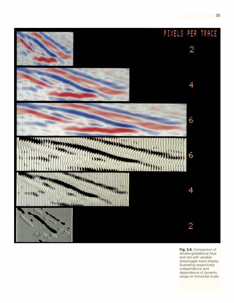
35

Fig. 2-9. Comparison ofdouble-gradational blueand red with variablearea/wiggle trace displayillustrating respectivelyindependence anddependence of dynamicrange on horizontal scale.

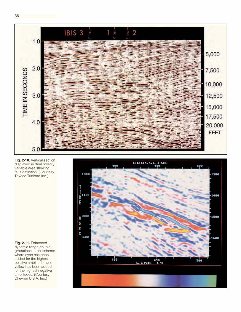
36

Fig. 2-10. Vertical sectiondisplayed in dual polarityvariable area showingfault definition. (CourtesyTexaco Trinidad Inc.)

Fig. 2-11. Enhanceddynamic range double-gradational color schemewhere cyan has beenadded for the highestpositive amplitudes andyellow has been addedfor the highest negativeamplitudes. (CourtesyChevron U.S.A. Inc.)

37

to the upper right to Line 122, Crossline 330. Is this a continuation of the channel sys-tem even though the amplitude is much reduced? We do not know the answer to thisquestion, but we have been able to observe the continuity of this extensive curvilin-ear feature because of the use of gradational color.

Figure 2-16 shows the same section in contrasting colors and the detectability of theinferred channel is much reduced. In fact the eye tends to be drawn to the red andpink circular maxima at Crossline 250 between Lines 45 and 60 rather than the longerarcuate high amplitude trends. When applying a gradational color scheme to a hori-zon slice showing the spatial amplitude distribution of one trough, as in Figure 2-15, agradational color scheme should be used to match the one-sided range of amplitudes.For the horizon slice for a peak (for example Figure 4-28) the same principle appliesbut the color scheme should be inverted. In order to aid the understanding of ampli-tudes, horizon slice colors should be matched to vertical section colors!

Fig. 2-12. Vertical sectiondisplayed with single-gradational gray scale inorder to enhance lowamplitude events.(Courtesy Texas PacificOil Company Inc.)

38

Fig. 2-13. Four differentcolor schemes applied tothe same vertical sectionsegment. (Courtesy TexasPacific Oil Company Inc.)

39

Fig. 2-14. Multiple colorschemes, some good andsome bad, for seismicdata.

A B C D E

F G H J K

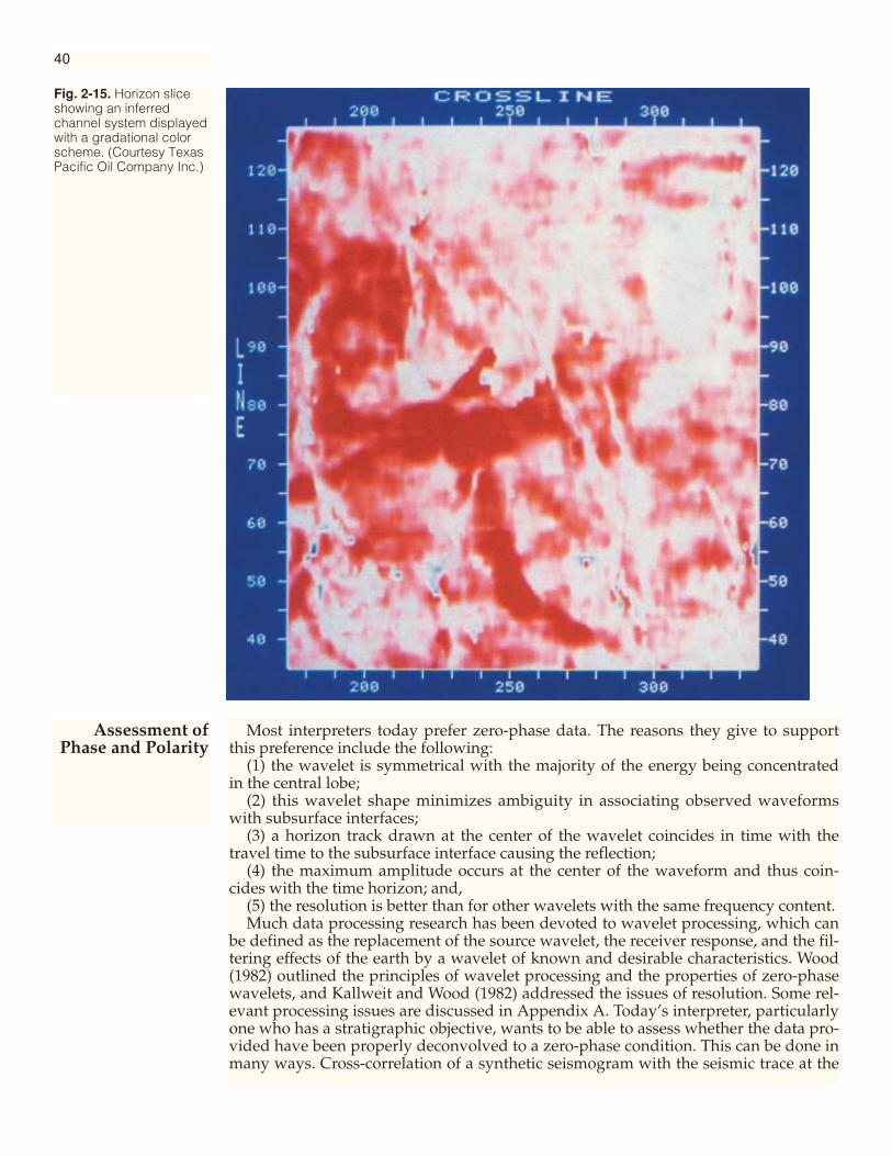
40

Most interpreters today prefer zero-phase data. The reasons they give to supportthis preference include the following:

(1) the wavelet is symmetrical with the majority of the energy being concentratedin the central lobe;

(2) this wavelet shape minimizes ambiguity in associating observed waveformswith subsurface interfaces;

(3) a horizon track drawn at the center of the wavelet coincides in time with thetravel time to the subsurface interface causing the reflection;

(4) the maximum amplitude occurs at the center of the waveform and thus coin-cides with the time horizon; and,

(5) the resolution is better than for other wavelets with the same frequency content.Much data processing research has been devoted to wavelet processing, which can

be defined as the replacement of the source wavelet, the receiver response, and the fil-tering effects of the earth by a wavelet of known and desirable characteristics. Wood(1982) outlined the principles of wavelet processing and the properties of zero-phasewavelets, and Kallweit and Wood (1982) addressed the issues of resolution. Some rel-evant processing issues are discussed in Appendix A. Today’s interpreter, particularlyone who has a stratigraphic objective, wants to be able to assess whether the data pro-vided have been properly deconvolved to a zero-phase condition. This can be done inmany ways. Cross-correlation of a synthetic seismogram with the seismic trace at the

Fig. 2-15. Horizon sliceshowing an inferredchannel system displayedwith a gradational colorscheme. (Courtesy TexasPacific Oil Company Inc.)

Assessment ofPhase and Polarity

41

Fig. 2-16. Same horizonslice as in Figure 2-15displayed with acontrasting color scheme,which reduces visibility ofthe channel system.(Courtesy Texas PacificOil Company Inc.)

well location is an analytical technique. So is the extraction of a wavelet from the dataand the study of its shape. But whatever is done, today’s interpreter needs anincreased awareness of zero-phaseness and the ability to recognize it, or other phases,in his or her data.

Understanding wavelet phase gives increased importance to the understanding ofpolarity. For processed seismic data, polarity convention is confused, and in additioncolor display introduces the need for conventions in color usage. In presenting aninterpretation using colored sections, the critical issue is to communicate the polarityand color usage for that data. It is less important what conventions are used becausepeaks and troughs are equally visible in color display. The author has developed asubjective appraisal of the polarity and color conventions in use today and these arediagrammed in Figure 2-17. American polarity is preferred in the Americas but is byno means universal in this region. European polarity is preferred in Europe and therest of the world but again is by no means universal there. If we are diligent in alwaysusing blue for positive amplitude and red for negative amplitude, then only twochoices remain. Are the data American or European polarity? This becomes a veryimportant, and hopefully straightforward, determination for today’s interpreter.

42

Fig. 2-18. Effect of phaseshifting constant phasewavelets.

Fig. 2-17. Polarity andcolor conventions, anddefinition of American andEuropean Polarity.

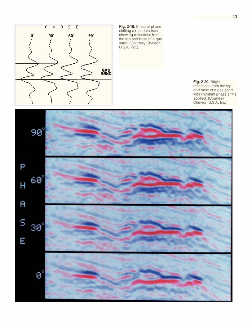
43

Fig. 2-19. Effect of phaseshifting a real data traceshowing reflections fromthe top and base of a gassand. (Courtesy ChevronU.S.A. Inc.)

Fig. 2-20. Brightreflections from the topand base of a gas sandwith constant phase shiftsapplied. (CourtesyChevron U.S.A. Inc.)

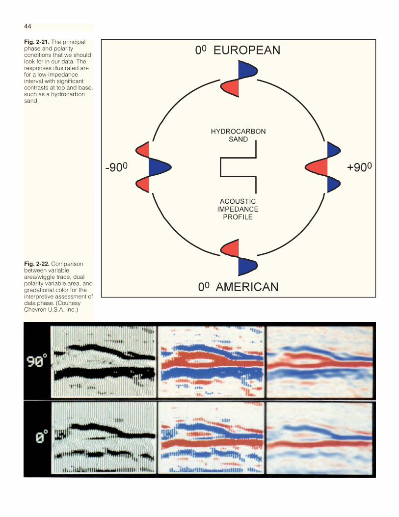
44

Fig. 2-22. Comparisonbetween variablearea/wiggle trace, dualpolarity variable area, andgradational color for theinterpretive assessment ofdata phase. (CourtesyChevron U.S.A. Inc.)

Fig. 2-21. The principalphase and polarityconditions that we shouldlook for in our data. Theresponses illustrated arefor a low-impedanceinterval with significantcontrasts at top and base,such as a hydrocarbonsand.

45

The interpretive assessment of zero-phaseness requires high signal-to-noise ratioreflections and maximum dynamic range color display. But first zero-phaseness willbe considered on model data. Figure 2-18 shows three zero-phase wavelets and theirequivalents shifted by 30, 60, and 90 degrees. The first is a Ricker wavelet, the secondis derived from a bandpass filter of 2.3 octaves with gentle slopes, and the third isderived from a bandpass filter of 1.3 octaves with steep slopes. The common propertyof these three wavelets is that the separation of central peak and first side lobe is thesame for each — 16 ms. The Ricker wavelet has no side lobes beyond the first. The 2.3octave wavelet is a good wavelet extracted from actual processed data and has lowside lobes. The 1.3 octave wavelet is a poor wavelet with relatively high side lobes.

The visual assessment of zero-phaseness amounts to a visual assessment of waveletsymmetry. In these model examples 30° of distortion is visible for all the wavelets butthe higher side lobe levels of the narrower band wavelet make the distortion less pro-nounced. For the larger distortions, for example at 60°, the central peak and the largerside lobe are more easily confused for the narrower band wavelet, so in practice itmay be difficult to decide whether the peak or the trough is the principal extremum.

Fig. 2-23. Use ofreflection strength orenvelope amplitude toobscure the effects ofphase distortion. (CourtesyChevron U.S.A. Inc.)

46

At a distortion of 90° the time horizon lies at the zero crossing between the largestamplitude peak and trough, and these are of equal size.

Figure 2-19 is a single trace example from real data where there was a known low-impedance gas sand. The top of the low-impedance zone is a peak and the base atrough (European polarity). The trace labelled 0° shows peak and trough each sym-metrically placed over their corresponding interfaces. The phase distortions are againevident when presented in this way.

In practice, interpreters must assess zero-phaseness on a section containing manytraces in case one trace is unrepresentative. We select a high amplitude reflection,which, on the basis of a simple model, can be related to a single interface. The inter-preter can then assume that the interference of events from adjacent parallel inter-faces, multiples or noise is small. Figure 2-20 illustrates a bright spot from a gas reser-voir where it is assumed that the above conditions hold except that there are twointerfaces at the top and at the base of the reservoir. In the panel labelled 0° there isone blue event from the top of the reservoir and one red event from its base, and theyhave approximately the same amplitude. Side lobes are low and symmetrical as far ascan be determined. This is the signature expected for the zero-phase response of a gassand.

For the 90° case in Figure 2-20 the top of the gas sand has a signature of blue-over-red and the base one of red-over-blue. This confirms the modeling illustrated in Fig-ure 2-18 and certainly shows a more complex character than the zero-phase section.The intermediate levels of phase distortion show the progression from the 0° to 90°condition. Observation of these more complicated phase characteristics can be fol-lowed by experimental phase rotation of the data.

Fig. 2-24. Flat spotreflection displaying zero-phaseness, visible ingradational red for manytraces and in wiggleformat for one trace.(Courtesy Chevron U.S.A.Inc.)

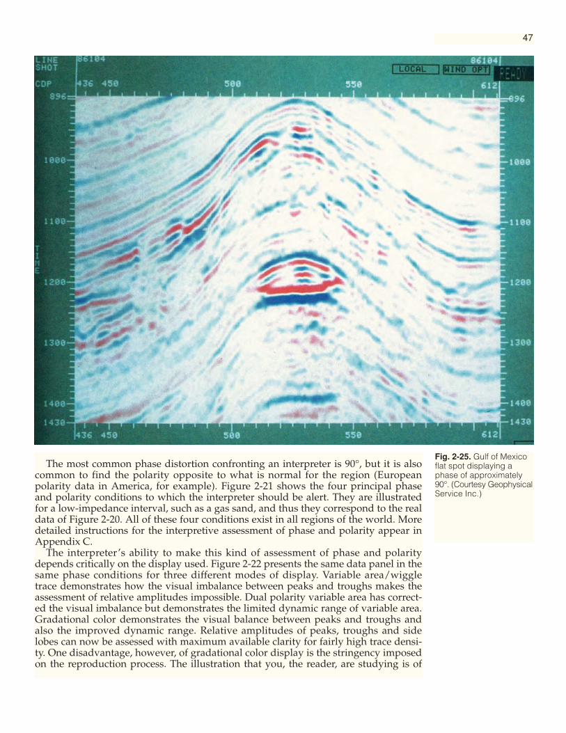
47

Fig. 2-25. Gulf of Mexicoflat spot displaying aphase of approximately90°. (Courtesy GeophysicalService Inc.)

The most common phase distortion confronting an interpreter is 90°, but it is alsocommon to find the polarity opposite to what is normal for the region (Europeanpolarity data in America, for example). Figure 2-21 shows the four principal phaseand polarity conditions to which the interpreter should be alert. They are illustratedfor a low-impedance interval, such as a gas sand, and thus they correspond to the realdata of Figure 2-20. All of these four conditions exist in all regions of the world. Moredetailed instructions for the interpretive assessment of phase and polarity appear inAppendix C.

The interpreter’s ability to make this kind of assessment of phase and polaritydepends critically on the display used. Figure 2-22 presents the same data panel in thesame phase conditions for three different modes of display. Variable area/wiggletrace demonstrates how the visual imbalance between peaks and troughs makes theassessment of relative amplitudes impossible. Dual polarity variable area has correct-ed the visual imbalance but demonstrates the limited dynamic range of variable area.Gradational color demonstrates the visual balance between peaks and troughs andalso the improved dynamic range. Relative amplitudes of peaks, troughs and sidelobes can now be assessed with maximum available clarity for fairly high trace densi-ty. One disadvantage, however, of gradational color display is the stringency imposedon the reproduction process. The illustration that you, the reader, are studying is of

48

Fig. 2-27. Gulf of Mexicoshallow gas reflectionsshowing a phase ofapproximately 90°.(Courtesy MobilExploration & ProducingU.S. Inc.)

Fig. 2-26. Subsurfacefeatures which cangenerate sufficiently highamplitude reflections to beuseful for interpretiveassessment of phase andpolarity. Probableimpedance profiles aredrawn.

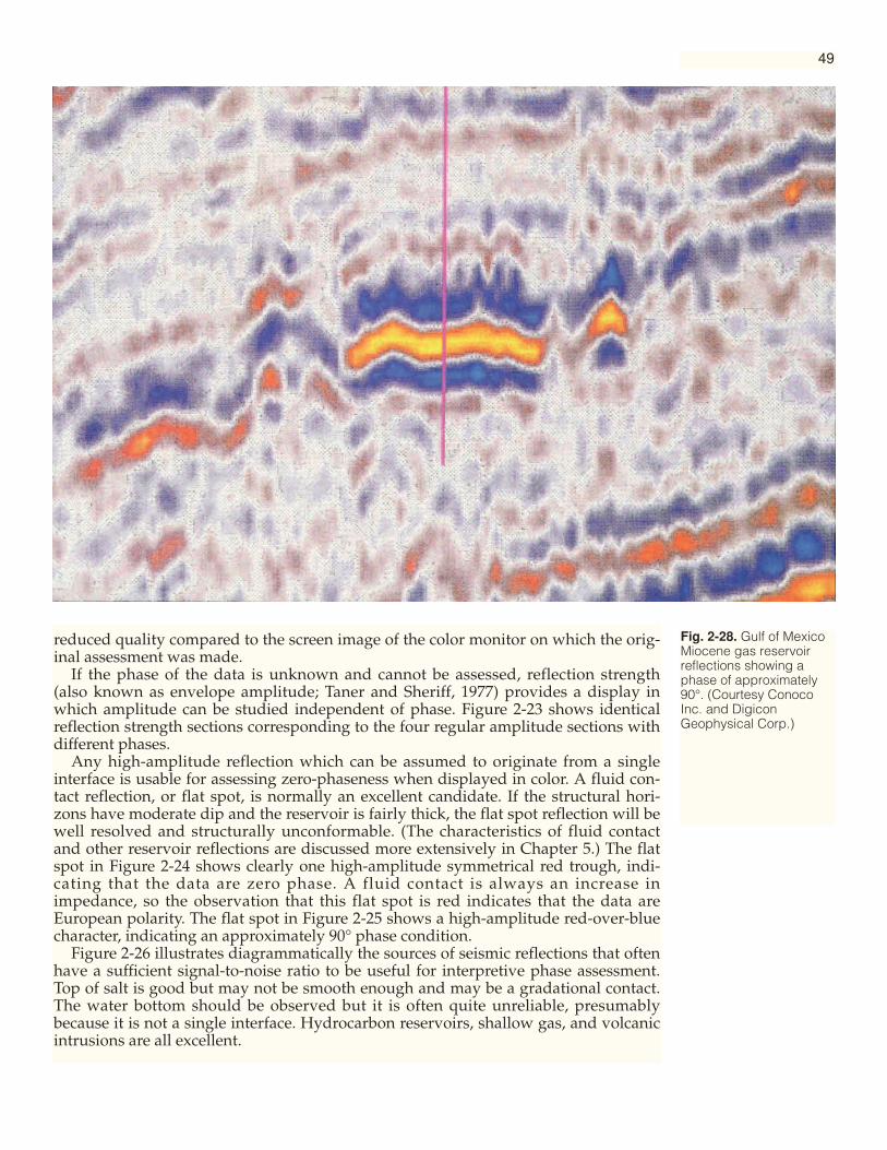
reduced quality compared to the screen image of the color monitor on which the orig-inal assessment was made.

If the phase of the data is unknown and cannot be assessed, reflection strength(also known as envelope amplitude; Taner and Sheriff, 1977) provides a display inwhich amplitude can be studied independent of phase. Figure 2-23 shows identicalreflection strength sections corresponding to the four regular amplitude sections withdifferent phases.

Any high-amplitude reflection which can be assumed to originate from a singleinterface is usable for assessing zero-phaseness when displayed in color. A fluid con-tact reflection, or flat spot, is normally an excellent candidate. If the structural hori-zons have moderate dip and the reservoir is fairly thick, the flat spot reflection will bewell resolved and structurally unconformable. (The characteristics of fluid contactand other reservoir reflections are discussed more extensively in Chapter 5.) The flatspot in Figure 2-24 shows clearly one high-amplitude symmetrical red trough, indi-cating that the data are zero phase. A fluid contact is always an increase inimpedance, so the observation that this flat spot is red indicates that the data areEuropean polarity. The flat spot in Figure 2-25 shows a high-amplitude red-over-bluecharacter, indicating an approximately 90° phase condition.

Figure 2-26 illustrates diagrammatically the sources of seismic reflections that oftenhave a sufficient signal-to-noise ratio to be useful for interpretive phase assessment.Top of salt is good but may not be smooth enough and may be a gradational contact.The water bottom should be observed but it is often quite unreliable, presumablybecause it is not a single interface. Hydrocarbon reservoirs, shallow gas, and volcanicintrusions are all excellent.

49

Fig. 2-28. Gulf of MexicoMiocene gas reservoirreflections showing aphase of approximately90°. (Courtesy ConocoInc. and DigiconGeophysical Corp.)

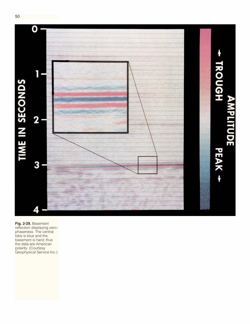
50

Fig. 2-29. Basementreflection displaying zero-phaseness. The centrallobe is blue and thebasement is hard; thusthe data are Americanpolarity. (CourtesyGeophysical Service Inc.)

Fig. 2-30. Water bottomreflection in deep waterdisplaying zero-phaseness and Europeanpolarity. (CourtesyConoco Inc.)

51

Figure 2-27 shows reflections from the top and base of shallow gas. Both are doubleevents indicating a phase of 90˚. Figure 2-28 shows strong reflections from a Miocenegas reservoir. Here the reservoir is thin so that the reflection from the top and thereflection from the bottom overlap each other, thus giving reinforcement of thered/yellow in the center. This again is an indication of 90˚ phase data, a remarkablycommon phenomenon.

Figure 2-29 shows an outstanding basement reflection which is probably from a sin-gle subsurface interface. The waveform of the reflection is clear, almost symmetrical,and spatially consistent. This indicates that the data are close to zero phase, at leastaround the time of 3 seconds (s). Figure 2-30 shows a strong water bottom reflection indeep water which is also a clear symmetrical waveform, again indicating zero-phase-ness. On top of the seamount the phase assessment is ambiguous but at the red arrowthe zero-phaseness is evident.

Time-variant phase distortion is possible but difficult to assess. Recently the authorwas able to determine that some Gulf of Mexico data were 90° at 2 s based on waterbottom and shallow gas, and zero-phase European polarity at 4 s based on poroussand, gas sand, and top salt.

A further and very good discussion on phase and polarity and their impact on theinterpreter is provided by Simm and White (2002).

Studies on the psychological impact of color have shown that hues of yellow,orange and red are advancing and attracting, while hues of green and blue are coolerand receding. The interpreter can take advantage of this in communicating his results.It would seem logical to display the structural highs, the isopach thicks and the ampli-tude highs in advancing colors in order to promote their prospectivity. Figure 2-6 is astructure map which demonstrates this point.

PsychologicalImpact of Color

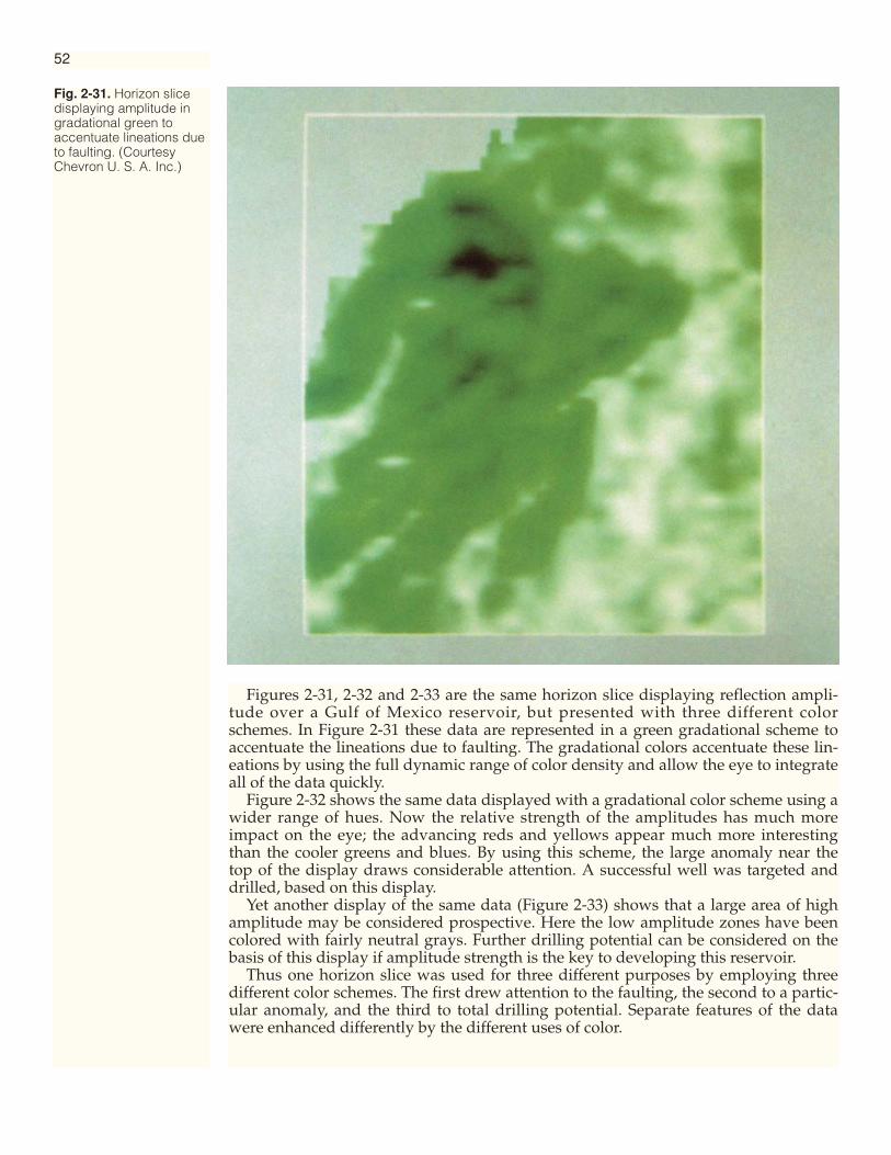
Figures 2-31, 2-32 and 2-33 are the same horizon slice displaying reflection ampli-tude over a Gulf of Mexico reservoir, but presented with three different colorschemes. In Figure 2-31 these data are represented in a green gradational scheme toaccentuate the lineations due to faulting. The gradational colors accentuate these lin-eations by using the full dynamic range of color density and allow the eye to integrateall of the data quickly.

Figure 2-32 shows the same data displayed with a gradational color scheme using awider range of hues. Now the relative strength of the amplitudes has much moreimpact on the eye; the advancing reds and yellows appear much more interestingthan the cooler greens and blues. By using this scheme, the large anomaly near thetop of the display draws considerable attention. A successful well was targeted anddrilled, based on this display.

Yet another display of the same data (Figure 2-33) shows that a large area of highamplitude may be considered prospective. Here the low amplitude zones have beencolored with fairly neutral grays. Further drilling potential can be considered on thebasis of this display if amplitude strength is the key to developing this reservoir.

Thus one horizon slice was used for three different purposes by employing threedifferent color schemes. The first drew attention to the faulting, the second to a partic-ular anomaly, and the third to total drilling potential. Separate features of the datawere enhanced differently by the different uses of color.

52

Fig. 2-31. Horizon slicedisplaying amplitude ingradational green toaccentuate lineations dueto faulting. (CourtesyChevron U. S. A. Inc.)

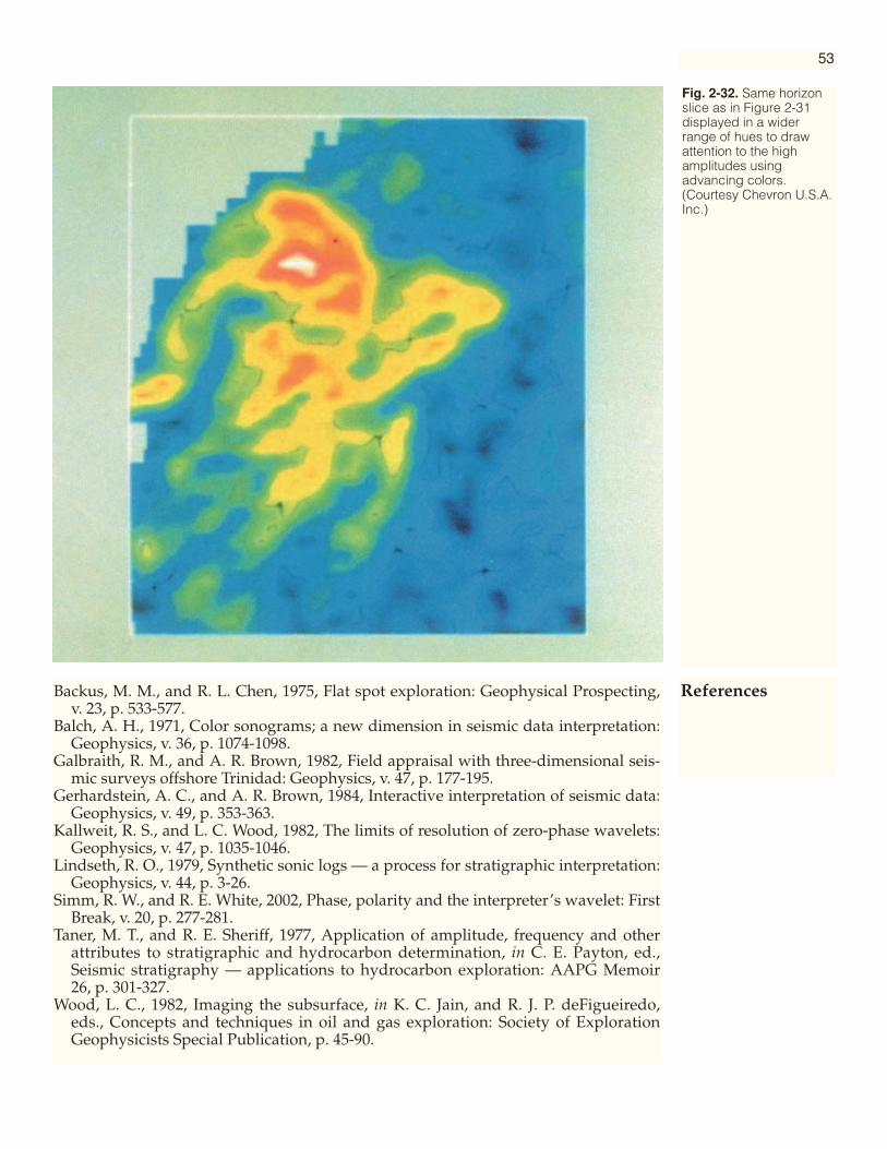
Backus, M. M., and R. L. Chen, 1975, Flat spot exploration: Geophysical Prospecting,v. 23, p. 533-577.

Balch, A. H., 1971, Color sonograms; a new dimension in seismic data interpretation:Geophysics, v. 36, p. 1074-1098.

Galbraith, R. M., and A. R. Brown, 1982, Field appraisal with three-dimensional seis-mic surveys offshore Trinidad: Geophysics, v. 47, p. 177-195.

Gerhardstein, A. C., and A. R. Brown, 1984, Interactive interpretation of seismic data:Geophysics, v. 49, p. 353-363.

Kallweit, R. S., and L. C. Wood, 1982, The limits of resolution of zero-phase wavelets:Geophysics, v. 47, p. 1035-1046.

Lindseth, R. O., 1979, Synthetic sonic logs — a process for stratigraphic interpretation:Geophysics, v. 44, p. 3-26.

Simm, R. W., and R. E. White, 2002, Phase, polarity and the interpreter’s wavelet: FirstBreak, v. 20, p. 277-281.

Taner, M. T., and R. E. Sheriff, 1977, Application of amplitude, frequency and otherattributes to stratigraphic and hydrocarbon determination, in C. E. Payton, ed.,Seismic stratigraphy — applications to hydrocarbon exploration: AAPG Memoir26, p. 301-327.

Wood, L. C., 1982, Imaging the subsurface, in K. C. Jain, and R. J. P. deFigueiredo,eds., Concepts and techniques in oil and gas exploration: Society of ExplorationGeophysicists Special Publication, p. 45-90.

53

References

Fig. 2-32. Same horizonslice as in Figure 2-31displayed in a widerrange of hues to drawattention to the highamplitudes usingadvancing colors.(Courtesy Chevron U.S.A.Inc.)

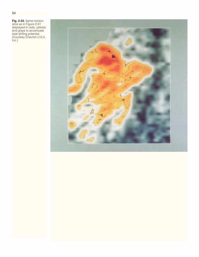
54

Fig. 2-33. Same horizonslice as in Figure 2-31displayed in reds, yellowsand grays to accentuatetotal drilling potential.(Courtesy Chevron U.S.A.Inc.)

55

Structural InterpretationThe 3-D seismic interpreter works with a volume of data. Normally this is done by

studying some of each of the three orthogonal slices through the volume. This chapterexplores the unique contribution of the horizontal section to structural interpretation.The interpreter of structure needs to be able to judge when to use horizontal sectionsand when to use vertical ones in the course of an overall interpretive project.

Figure 3-1 demonstrates the conceptual relationship between a volume of subsur-face rock and a volume of seismic data. Consider the diagram first to represent sub-surface rocks and the gray surface to be a bedding plane. The two visible verticalfaces of the rectangular solid show the two dip components of the plane; the horizon-tal face shows the strike of the plane. Now consider the rectangular solid of Figure 3-1to be the equivalent volume of seismic data. The gray plane is now a dipping reflec-tion and its intersections with the three orthogonal faces of the solid show the twocomponents of dip and the strike as before. Hence the attitude of a reflection on a hor-izontal section indicates directly the strike of the reflecting surface. This is the funda-mental property of the horizontal section from which all its unique interpretive valuederives.

Contours follow strike and indicate a particular level in time or depth. When aninterpreter picks a reflection on a horizontal section, it is directly a contour on somehorizon at the time (or depth) at which the horizontal section was sliced through thedata volume.

Figure 3-2 shows three horizontal sections, four milliseconds apart. By followingthe semicircular black event (peak) from level to level and drawing contours at anappropriate interval, the structural contour map at the bottom of Figure 3-2 was gen-erated. Note the similarity in shape between the sections and the map for the anticli-nal structure and the strike east of the faults. In the central panel the peaks from 1352ms are printed in black and the peaks from 1360 ms in blue/green. This clearlydemonstrates the way in which the events have moved with depth.

Figures 3-3 and 3-5 provide one vertical section and several horizontal sectionsfrom which the relationship between the two perspectives can be appreciated. Line P(Figure 3-3) runs north-south through the middle of the prospect with south at theright. The time interval 2632-2656 ms shows some continuous reflections. Proceedingfrom south to north (right to left, Figure 3-3; bottom to top, Figure 3-5) the structure isfirst a broad closed anticline, then a shoulder, then a smaller anticline.

Figure 3-5 demonstrates a simple exercise in direct contouring from a suite of hori-zontal sections. The red event (trough) expanding in size from left to right has beenprogressively circumscribed in the lower part of the figure. The last frame is a rawcontour map of this horizon. This first structural representation has been made quickly

Direct Contouringand theImportance of theStrike Perspective

CHAPTER THREE

56

and efficiently without the traditional intermediate tasks of timing, posting and con-touring. When drawing structural contours from horizontal sections in this way, it iswise to visualize the three-dimensionality of the structure and to appreciate where onthe seismic waveform the contour is being drawn (Figure 3-4). The latter problemapplies particularly to the use of variable area displays as used, for example, in Figure3-5. The contour is here drawn all the way around the red event only because the dipis down all the way around the structure; this is a consistent point on the seismicwaveform, namely its upper edge (Figure 3-4).

Figure 3-6 shows 24 horizontal sections covering an area of about 5 sq mi (13 sqkm). These can be used as a structural interpretation exercise. Obtain a small piece oftransparent paper and register it over the rectangular area. Begin with the upper leftframe and find the red event in its lower right corner. Mark this event by following itsmaximum amplitude and then mark its changed position from frame to frame untilyou reach 2160 ms. Your resultant contour map should show that the dip is generallynorthwest and that the strike swings about 40° toward the north over the structuralrange of the map. You will probably detect a fault toward the west of the area as well.If you study the arcuate events west of the fault, you will recognize a small anticlineclosing against the fault and a small syncline south of it. There is no way to establishthe correlation across the fault.

An event on a horizontal section is generally broader than on a vertical section asdips are usually less than 45°. Figure 3-7 shows the effect of dip and frequency on thewidth of an event on a horizontal section. A gently dipping event is very broad and asteeply dipping event is much narrower. Increasing dip and increasing frequencyboth make horizontal section events narrower. The width of an event on a horizontalsection is strictly half the spatial wavelength.

Because typical dips are much less than 45°, fewer horizontal sections than verticalones are needed to study the full extent of a reflection within a given data volume. Thisgives horizontal sections greater efficiency than vertical sections in structural mapping.Combining this benefit with the fact that horizon tracks (picks) are directly contours,then the value of horizontal sections to structural interpretation is substantial.

Fig. 3-1. Relationbetween dip and strike ofa seismic reflector withina data volume.

Text continues on page 67

57

Fig. 3-2. Dual polarity horizontal sections from offshore Holland; two-level single polarity horizontal section, showing movement of eventsfrom 1352 ms to 1360 ms; interpreted contour map on horizon seen asstrongest event on horizontal sections.

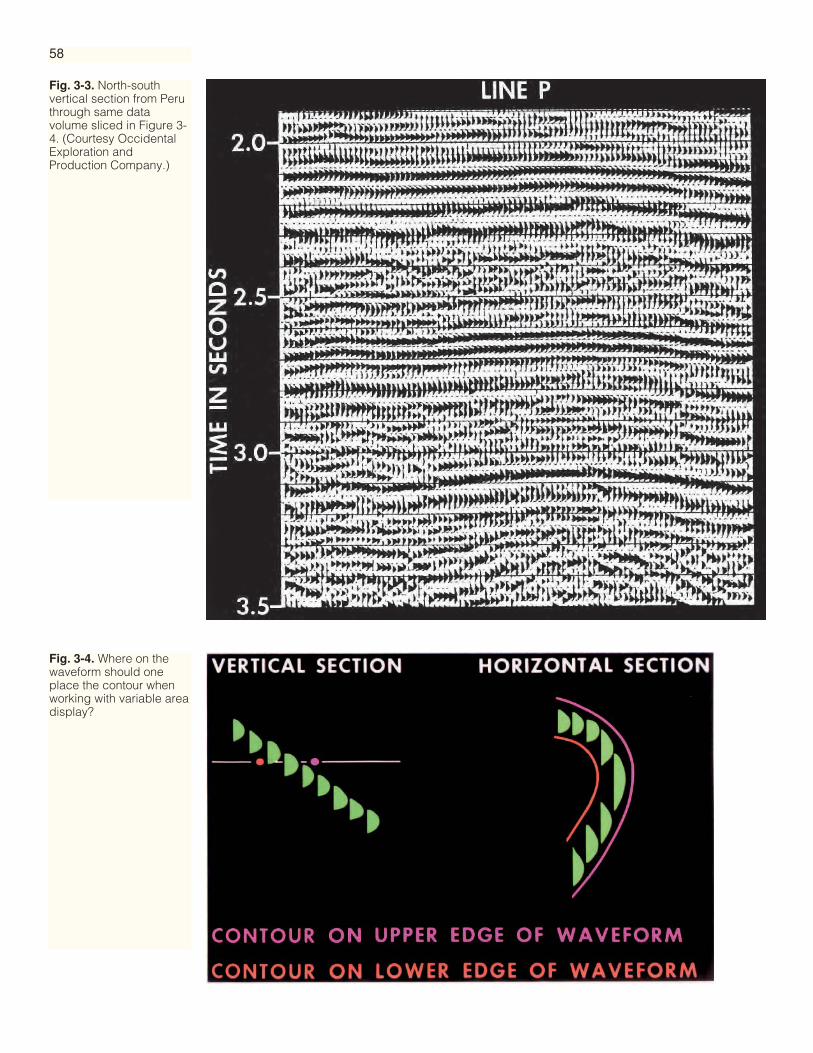
58

Fig. 3-3. North-southvertical section from Peruthrough same datavolume sliced in Figure 3-4. (Courtesy OccidentalExploration andProduction Company.)

Fig. 3-4. Where on thewaveform should oneplace the contour whenworking with variable areadisplay?

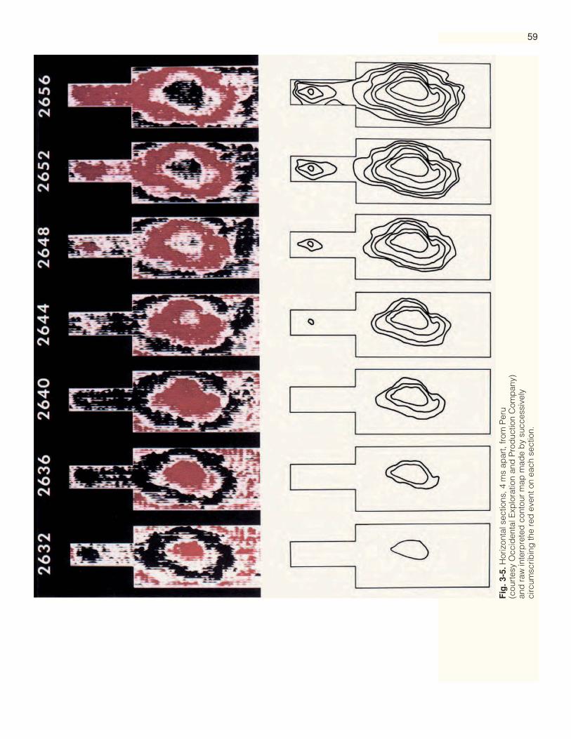
59

Fig

. 3-5

.Hor

izon

tal s

ectio

ns, 4

ms

apar

t, fr

om P

eru

(cou

rtes

y O

ccid

enta

l Exp

lora

tion

and

Pro

duc

tion

Com

pan

y)an

d r

aw in

terp

rete

d c

onto

ur m

ap m

ade

by

succ

essi

vely

circ

umsc

ribin

g th

e re

d e

vent

on

each

sec

tion.

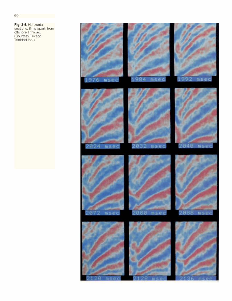
60

Fig. 3-6. Horizontalsections, 8 ms apart, fromoffshore Trinidad.(Courtesy TexacoTrinidad Inc.)

61

62

Fig. 3-7. The width of anevent on a horizontalsection decreases withincreased dip and alsowith increased frequency.

63

Fig

. 3-8

.Str

uctu

ral c

onto

ur m

apd

eriv

ed fr

om 2

-D d

ata

from

the

Gul

f of T

haila

nd. (

Cou

rtes

y Te

xas

Pac

ific

Oil

Com

pan

y In

c.)

Fig

. 3-9

.Str

uctu

ral c

onto

ur m

apd

eriv

ed fr

om 3

-D d

ata

from

the

Gul

f of T

haila

nd fo

r th

e sa

me

horiz

on m

app

ed in

Fig

ure

3-8.

(Cou

rtes

y Te

xas

Pac

ific

Oil

Com

pan

y In

c.)

64F

ig. 3

-11.

Str

uctu

ral c

onto

urm

ap d

eriv

ed fr

om 3

-D d

ata

from

offs

hore

Chi

le fo

r th

e sa

me

horiz

on m

app

ed in

Fig

ure

3-10

.(C

ourt

esy

EN

AP

).

Fig

. 3-1

0.S

truc

tura

l con

tour

map

der

ived

from

2-D

dat

afr

om o

ffsho

re C

hile

. (C

ourt

esy

EN

AP

).

65

Fig. 3-12. Line 55 fromGulf of Thailand 3-D data.(Courtesy Texas PacificOil Company Inc.)

Fig. 3-13. Horizontalsection at 1388 msfrom Gulf of Thailand.(Courtesy TexasPacific Oil Company.)

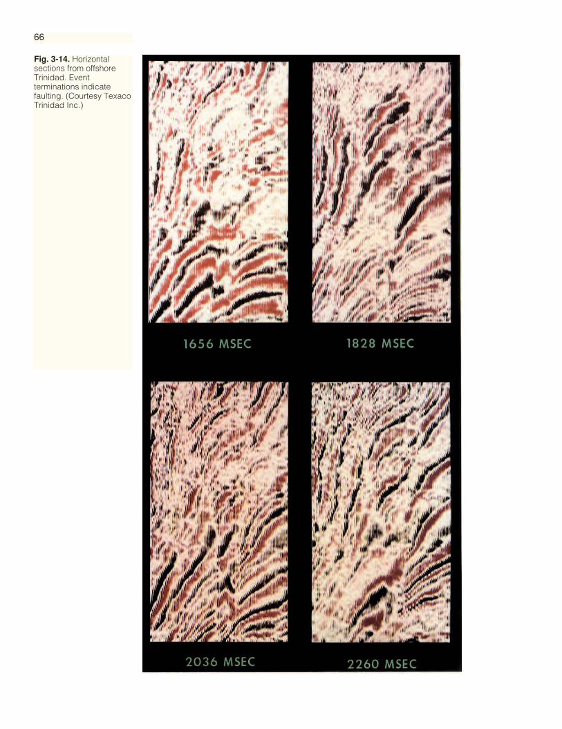
66

Fig. 3-14. Horizontalsections from offshoreTrinidad. Eventterminations indicatefaulting. (Courtesy TexacoTrinidad Inc.)

67

When an interpreter works with 3-D data after having previously mapped from 2-Ddata over the same prospect, the most striking difference between maps is commonlythe increased fault detail in the 3-D map. Figures 3-8 and 3-9 provide a typical compar-ison and also demonstrate increased detail in the shape of the structural contours.Comparison of Figures 3-10 and 3-11 also shows a considerable increase in the numberof faults and in the structural detail. The three well locations indicated in blue appearstructurally quite different on the 2-D and 3-D maps.

We expect to detect faults from alignments of event terminations. Figure 3-12shows a vertical section from the 3-D data which provided the map of Figure 3-9. Theevent terminations clearly show several faults. The horizontal section of Figure 3-13 isfrom the same data volume and, in contrast, does not show clear event terminations.Figure 3-14 shows four horizontal sections from a different prospect but one in a simi-lar tertiary clastic environment. Here event terminations clearly indicate the positionsof three major faults on each of the four sections.

Why are event terminations visible at the faults in Figure 3-14 but not in Figure 3-13? The answer lies simply in the relationship between structural strike and faultstrike. Any horizontal section alignment indicates the strike of the feature. If there is asignificant angle between structural strike and fault strike, the events will terminate.

Fig. 3-15. Horizontalsection from onshoreEurope. Eventterminations indicatefaulting.

Fault Recognitionand Mapping

68

Fig. 3-16. Horizontalsection at 1500 ms fromGulf of Mexico showingmany clearly visible faults.At least 10 areidentifiable. (CourtesyConoco Inc. and TexacoU.S.A. Inc.)

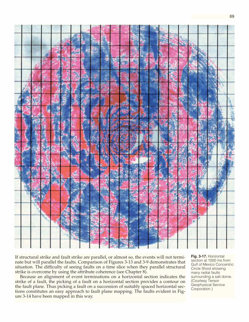
69

If structural strike and fault strike are parallel, or almost so, the events will not termi-nate but will parallel the faults. Comparison of Figures 3-13 and 3-9 demonstrates thatsituation. The difficulty of seeing faults on a time slice when they parallel structuralstrike is overcome by using the attribute coherence (see Chapter 8).

Because an alignment of event terminations on a horizontal section indicates thestrike of a fault, the picking of a fault on a horizontal section provides a contour onthe fault plane. Thus picking a fault on a succession of suitably spaced horizontal sec-tions constitutes an easy approach to fault plane mapping. The faults evident in Fig-ure 3-14 have been mapped in this way.

Fig. 3-17. Horizontalsection at 1000 ms fromGulf of Mexico ConcentricCircle Shoot showingmany radial faultssurrounding a salt dome.(Courtesy TensorGeophysical ServiceCorporation.)

70

In the lower right corner of the horizontal section at 2260 ms (Figure 3-14) two faultblocks show events of quite different widths. This is the effect of dip which wasexplained by Figure 3-7. We also see a similar effect of dip in Figure 3-13 where thefaults are mostly traced by narrow sinuous events striking approximately north-south.

Figure 3-15 shows a variety of structural features: prominent faults, more subtlefaults, culminations, and various character changes. It is very important that horizon-tal sections play their proper role in fault interpretation. In the early stages of struc-tural interpretation of a prospect, the major faults will be identified on some widely-spaced vertical sections. The way in which these faults join up into a fault frameworkshould then be established from horizontal sections. This is part of the overall recom-mended procedure of Figure 3-32. Lineations of event terminations will normally linkthe faults already recognized vertically. Figures 3-16 and 3-17 show clearly visiblefaulting that evidently could be used in this way.

Today’s interactive workstations help in the coordinated use of vertical and hori-zontal sections by providing the capability of cross-posting. When a fault is picked ona vertical section, its intersection will appear on an intersecting horizontal section.

Fig. 3-18. Horizontalsection at 3252 ms fromEugene Island area ofGulf of Mexico showinginterpreted shape of saltplug. (Courtesy Hunt OilCompany.)

71

Fig. 3-19. Horizontalsection at 3760 ms fromEugene Island area ofGulf of Mexico. (CourtesyHunt Oil Company.)

Fig. 3-20. Samehorizontal section asFigure 3-19 withinterpretation of faults andthe green horizon.(Courtesy Hunt OilCompany.)

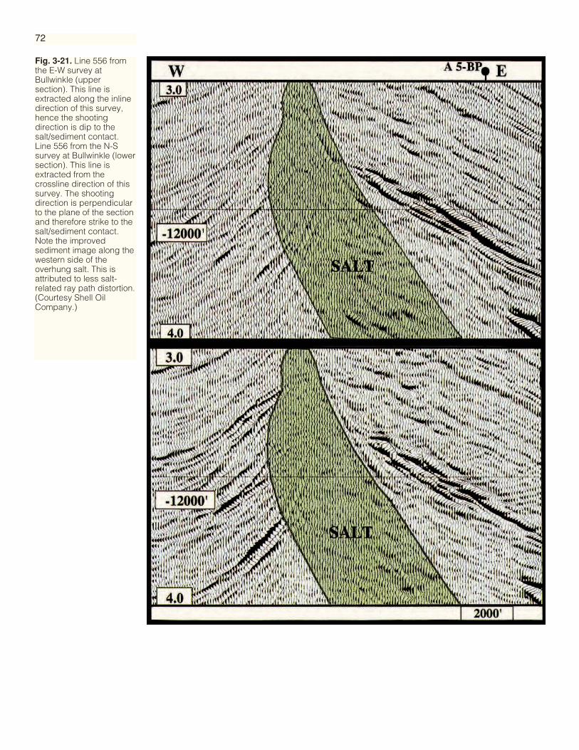
72

Fig. 3-21. Line 556 fromthe E-W survey atBullwinkle (uppersection). This line isextracted along the inlinedirection of this survey,hence the shootingdirection is dip to thesalt/sediment contact.Line 556 from the N-Ssurvey at Bullwinkle (lowersection). This line isextracted from thecrossline direction of thissurvey. The shootingdirection is perpendicularto the plane of the sectionand therefore strike to thesalt/sediment contact.Note the improvedsediment image along thewestern side of theoverhung salt. This isattributed to less salt-related ray path distortion.(Courtesy Shell OilCompany.)

73

Fig. 3-22. Time slice 1500ms from a circular 3-Dsurvey in the North Sea. Theshattered appearanceresults from the shattering ofa thin limestone. (CourtesyMobil North Sea Limited.)

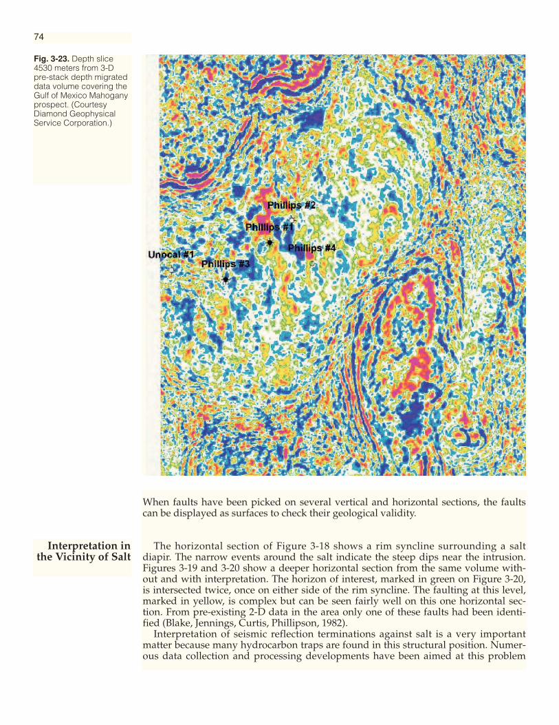
Fig. 3-23. Depth slice4530 meters from 3-Dpre-stack depth migrateddata volume covering theGulf of Mexico Mahoganyprospect. (CourtesyDiamond GeophysicalService Corporation.)

74

When faults have been picked on several vertical and horizontal sections, the faultscan be displayed as surfaces to check their geological validity.

The horizontal section of Figure 3-18 shows a rim syncline surrounding a saltdiapir. The narrow events around the salt indicate the steep dips near the intrusion.Figures 3-19 and 3-20 show a deeper horizontal section from the same volume with-out and with interpretation. The horizon of interest, marked in green on Figure 3-20,is intersected twice, once on either side of the rim syncline. The faulting at this level,marked in yellow, is complex but can be seen fairly well on this one horizontal sec-tion. From pre-existing 2-D data in the area only one of these faults had been identi-fied (Blake, Jennings, Curtis, Phillipson, 1982).

Interpretation of seismic reflection terminations against salt is a very importantmatter because many hydrocarbon traps are found in this structural position. Numer-ous data collection and processing developments have been aimed at this problem

Interpretation inthe Vicinity of Salt

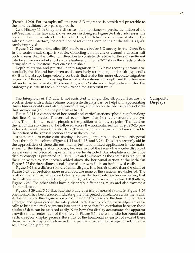
(French, 1990). For example, full one-pass 3-D migration is considered preferable tothe more traditional two-pass approach.

Case History 11 in Chapter 9 discusses the importance of precise definition of thesalt/sediment interface and shows success in doing so. Figure 3-21 also addresses thisissue and demonstrates that, by collecting the data in a direction strike to thesalt/sediment interface, the definition of reflections terminating at the salt is signifi-cantly improved.

Figure 3-22 shows time slice 1500 ms from a circular 3-D survey in the North Sea.In the center a salt diapir is visible. Collecting data in circles around a circular saltbody means that the collection direction is consistently strike to the salt/sedimentinterface. The myriad of short arcuate features on Figure 3-22 show the effects of shat-tering of a thin limestone layer encased in shale.

Depth migration and pre-stack depth migration in 3-D have recently become eco-nomically feasible and have been used extensively for imaging under salt (AppendixA). It is the abrupt large velocity contrasts that make this more elaborate migrationnecessary. After such processing the whole data volume is in depth and thus horizon-tal sections become depth slices. Figure 3-23 shows a depth slice under theMahogany salt sill in the Gulf of Mexico and the successful wells.

The interpreter of 3-D data is not restricted to single slice displays. Because thework is done with a data volume, composite displays can be helpful in appreciatingthree-dimensionality and also in concentrating attention on the precise pieces of datathat provide insight into the problem at hand.

Figure 3-24 is a composite of horizontal and vertical sections spliced together alongtheir line of intersection. The vertical section shows that the circular structure is a syn-cline. The horizontal section pinpoints the position of its lowest point. The fault onthe left of this structure can be followed across the horizontal section. Figure 3-25 pro-vides a different view of the structure. The same horizontal section is here spliced tothe portion of the vertical section above in the volume.

It is possible to make cube displays showing, simultaneously, three orthogonalslices through the volume (Figures 1-14 and 1-15, and 3-26). These can certainly aid inthe appreciation of three-dimensionality but have limited application in the main-stream of the interpretation process, because two of the faces of any cube displayedon a monitor or piece of paper will always be distorted. An adaptation of the cubedisplay concept is presented in Figure 3-27 and is known as the chair; it is really justthe cube with a vertical section added above the horizontal section at the back. OnFigure 3-27 the three-dimensional shape of a growth fault can be followed easily.

Figure 3-28 is a different kind of chair display. It is less dramatic than the chair ofFigure 3-27 but probably more useful because none of the sections are distorted. Thefault on the left can be followed clearly across the horizontal section indicating thatthe fault visible on line 75 (top, Figure 3-28) is the same as seen on line 110 (bottom,Figure 3-28). The other faults have a distinctly different azimuth and also traverse ashorter distance.

Figures 3-29 and 3-30 illustrate the study of a trio of normal faults. In Figure 3-29one horizon has been tracked indicating the interpreted correlation across the faults.At the bottom of this figure a portion of the data from each of the four fault blocks isenlarged and again carries the interpreted track. Each block has been adjusted verti-cally to bring the track segments into continuity so that the correlation between theseblocks of data can be assessed easily. Note how this display accentuates the apparentgrowth on the center fault of the three. In Figure 3-30 the composite horizontal andvertical section display permits the study of the horizontal extension of each of thesethree faults. A display customized to a problem usually helps significantly in thesolution of that problem.

75

CompositeDisplays

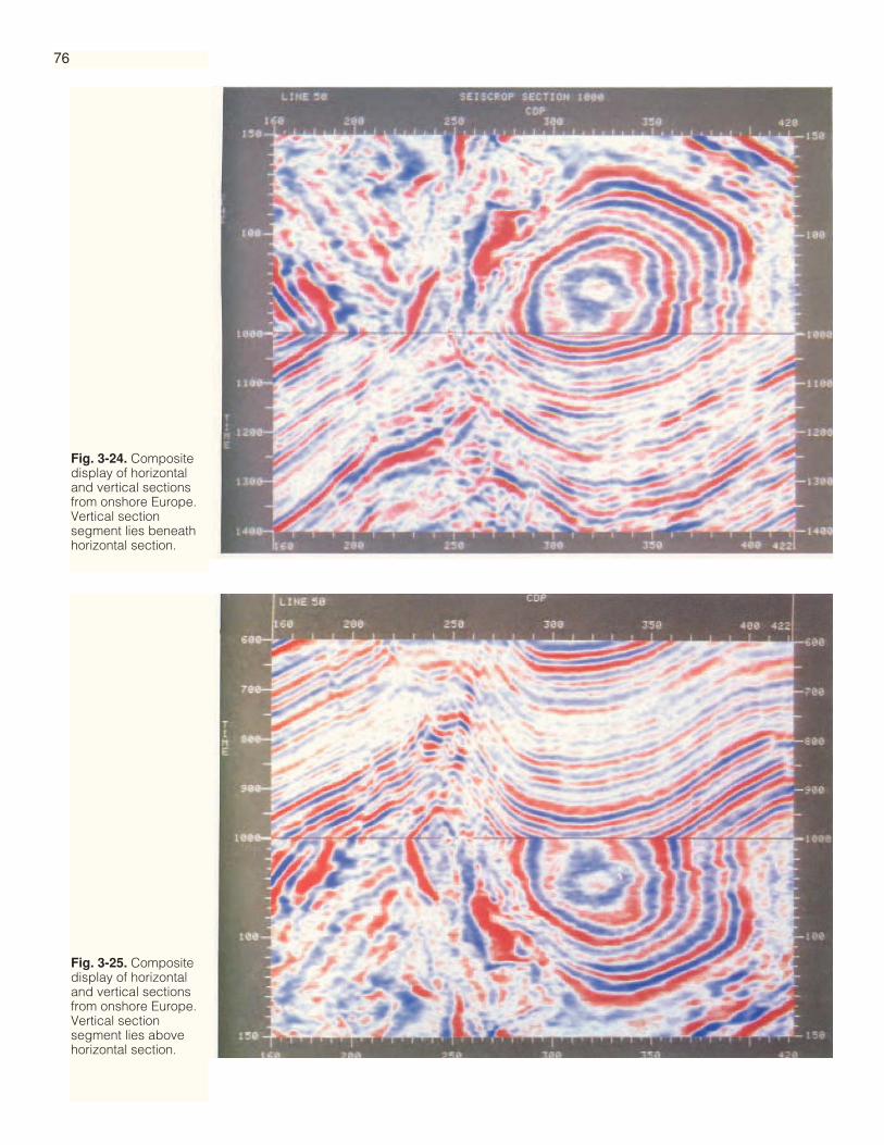
76

Fig. 3-24. Compositedisplay of horizontaland vertical sectionsfrom onshore Europe.Vertical sectionsegment lies beneathhorizontal section.

Fig. 3-25. Compositedisplay of horizontaland vertical sectionsfrom onshore Europe.Vertical sectionsegment lies abovehorizontal section.

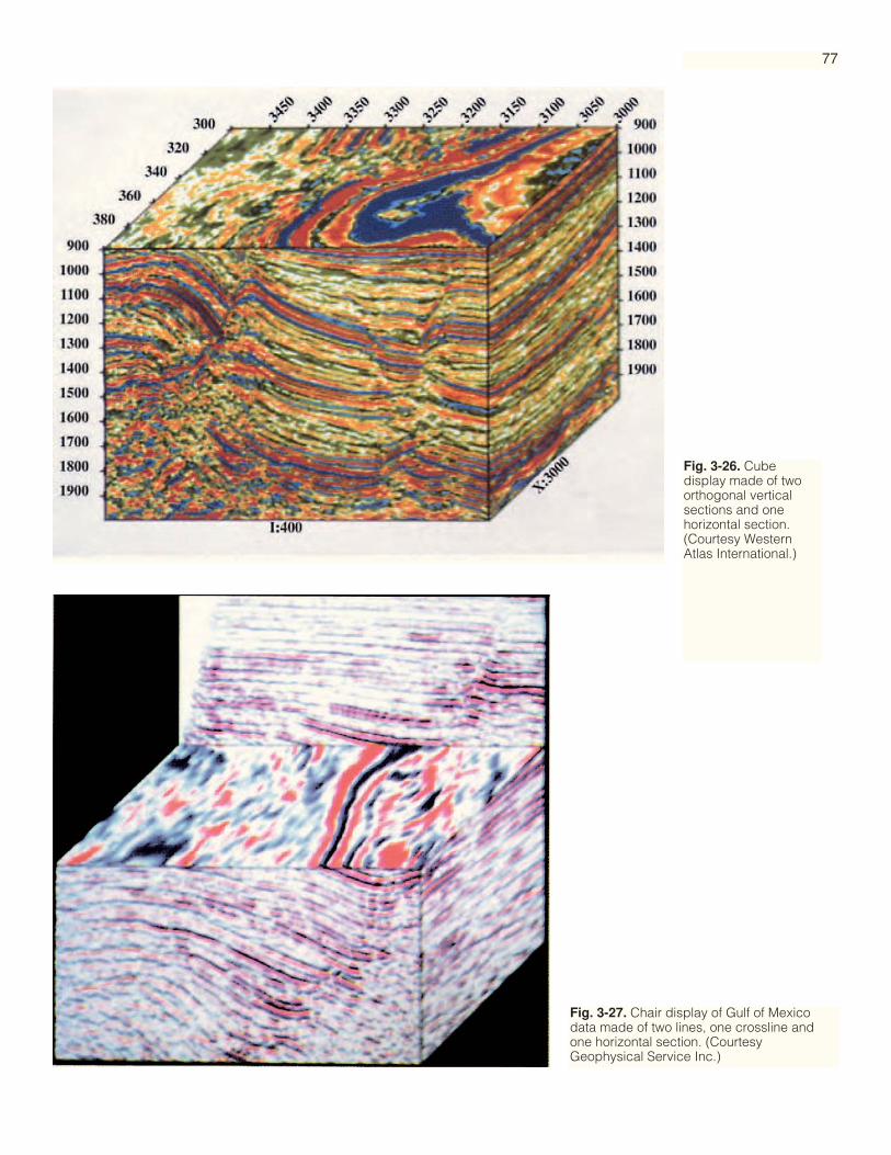
77

Fig. 3-26. Cubedisplay made of twoorthogonal verticalsections and onehorizontal section.(Courtesy WesternAtlas International.)

Fig. 3-27. Chair display of Gulf of Mexicodata made of two lines, one crossline andone horizontal section. (CourtesyGeophysical Service Inc.)

78

Fig. 3-28. Chair display made of two vertical sections and one horizontal section. Compare this with Figure 3-27 and note that hereall the three sections are undistorted. (Courtesy Landmark Graphics Corporation.)

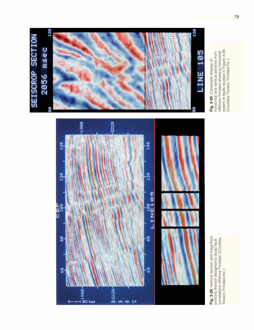
79

Fig

. 3-2

9.V

ertic

al s

ectio

n an

d m

agni

fied

por

tions

ther

eof d

esig

ned

to s

tud

y fa

ult

corr

elat

ions

offs

hore

Trin

idad

. (C

ourt

esy

Texa

co T

rinid

ad In

c.)

Fig

. 3-3

0.C

omp

osite

dis

pla

y of

horiz

onta

l and

ver

tical

sec

tions

from

offs

hore

Trin

idad

sho

win

g h

oriz

onta

lex

tent

of f

aults

stu

die

d in

Fig

ure

3-28

.(C

ourt

esy

Texa

co T

rinid

ad In

c.)

80

Fig

. 3-3

1.S

urfa

ce s

lices

from

sou

th T

exas

in ti

me

and

am

plit

ude,

and

thei

r eq

uiva

lent

time

slic

es. T

he s

urfa

ces

slic

es a

re 6

ms

thic

k an

d v

ertic

ally

ad

jace

nt s

lices

are

sep

-ar

ated

by

6 m

s. (

Cou

rtes

y E

xxon

Pro

duc

tion

Res

earc

h C

omp

any.

)

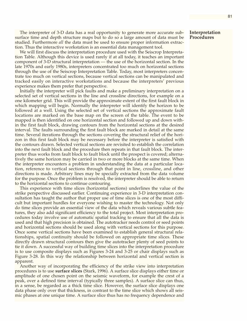
81

The interpreter of 3-D data has a real opportunity to generate more accurate sub-surface time and depth structure maps but to do so a large amount of data must bestudied. Furthermore all the data must be used to ensure proper information extrac-tion. Thus the interactive workstation is an essential data management tool.

We will first discuss the interpretation procedure used with the Seiscrop Interpreta-tion Table. Although this device is used rarely if at all today, it teaches an importantcomponent of 3-D structural interpretation — the use of the horizontal section. In thelate 1970s and early 1980s, interpreters concentrated too much on horizontal sectionsthrough the use of the Seiscrop Interpretation Table. Today, most interpreters concen-trate too much on vertical sections, because vertical sections can be manipulated andtracked easily on interactive workstations and because the interpreters’ previousexperience makes them prefer that perspective.

Initially the interpreter will pick faults and make a preliminary interpretation on aselected set of vertical sections in the line and crossline directions, for example on aone kilometer grid. This will provide the approximate extent of the first fault block inwhich mapping will begin. Normally the interpreter will identify the horizon to befollowed at a well. Using the selected set of vertical sections the approximate faultlocations are marked on the base map on the screen of the table. The event to bemapped is then identified on one horizontal section and followed up and down with-in the first fault block, drawing contours from the horizontal sections at the desiredinterval. The faults surrounding the first fault block are marked in detail at the sametime. Several iterations through the sections covering the structural relief of the hori-zon in this first fault block may be necessary before the interpreter is satisfied withthe contours drawn. Selected vertical sections are revisited to establish the correlationinto the next fault block and the procedure then repeats in that fault block. The inter-preter thus works from fault block to fault block until the prospect is covered; alterna-tively the same horizon may be carried in two or more blocks at the same time. Whenthe interpreter encounters a problem in understanding the data at a particular loca-tion, reference to vertical sections through that point in line, crossline, and otherdirections is made. Arbitrary lines may be specially extracted from the data volumefor the purpose. Once the problem is resolved, the interpreter should be able to returnto the horizontal sections to continue contouring.

This experience with time slices (horizontal sections) underlines the value of thestrike perspective discussed earlier. Continuing experience in 3-D interpretation con-sultation has taught the author that proper use of time slices is one of the most diffi-cult but important hurdles for everyone wishing to master the technology. Not onlydo time slices provide an essential view of the data which reveals various subtle fea-tures, they also add significant efficiency to the total project. Most interpretation pro-cedures today involve use of automatic spatial tracking to ensure that all the data isused and that high precision is obtained. The autotracker needs control or seed pointsand horizontal sections should be used along with vertical sections for this purpose.Once some vertical sections have been examined to establish general structural rela-tionships, spatial continuity should be followed on appropriate time slices. Thesedirectly drawn structural contours then give the autotracker plenty of seed points totie it down. A successful way of building time slices into the interpretation procedureis to use composite displays such as Figures 3-24 and 3-25 or chair displays such asFigure 3-28. In this way the relationship between horizontal and vertical section isapparent.

Another way of incorporating the efficiency of the strike view into interpretationprocedures is to use surface slices (Stark, 1996). A surface slice displays either time oramplitude of one chosen point on the seismic waveform, for example the crest of apeak, over a defined time interval (typically three samples). A surface slice can thus,in a sense, be regarded as a thick time slice. However, the surface slice displays onedata phase only over that thickness, in contrast to the time slice which shows all seis-mic phases at one unique time. A surface slice thus has no frequency dependence and

InterpretationProcedures

provides true dip magnitude. Figure 3-31 contains a sequence of time slices and theequivalent amplitude surface slices and time surface slices. The surface slices are 6 msthick and contain only peaks, either their horizon amplitudes or their travel times.Slices on the same row are from the same time, and the rows are separated by 6 ms.Vertically adjacent surface slices are thus independent and it can be seen that theedges of the colored areas fit together. This is the procedure with surface slices — akind of jigsaw puzzle of horizon segments.

Figure 3-32 charts a recommended procedure for 3-D interpretation using an inter-active workstation. The interactive capabilities required to follow this procedureinclude:

(1) automatic and manual tracking of horizons on vertical and horizontal sections;(2) automatic spatial horizon tracking and editing through a 3-D data volume;(3) correlation of vertical sections with well data;(4) extraction, storing and manipulation of seismic amplitudes;(5) manipulation of maps;(6) flexible use of color; and(7) extraction and use of seismic attributes.

This approach incorporates many of the notions from the previous procedures bututilizes the greatly extended capabilities. The procedure of Figure 3-32 also addresses

82

RECOMMENDED PROCEDURE

1. Preview of data on composite displays and movies.

2. Horizon identification at wells.Assessment of data phase and polarity.

3. Recognition of major faults on widely-spaced vertical sections.

4. Fault framework by tying together with horizontal sections.

5. Initial horizon control using vertical and horizontal sections.Horizontal sections provide efficiency of coverage.

6. Automatic spatial tracking to complete horizon on every point.Autotracking provides precision picking.

Get to this point as quickly as possible.

7. Scrutiny of intermediate horizon products for new features and for validation of tracking:

Color-posted time structure (including lineations of untracked points)Color-posted horizon slice (for lineations and patterns in amplitude)High spatial frequency residualDip magnitude and azimuth, difference, edge detection and illumination

8. Revision of horizons and faults, and rerun of autotracking.

9. Final time structure maps and horizon slices with chosen amounts of gridding orsmoothing.

10. Isochron, isopach and depth maps.

11. Detailed stratigraphic and reservoir studies.

Fig. 3-32. Recommendedinteractive 3-Dinterpretation procedure.

several areas of stratigraphic and reservoir interpretation which will be discussed inlater chapters.

Some of the important principles implicit in the procedure of Figure 3-32 are thatyou

• understand the phase of data before embarking on the mainstream interpretation,• use horizontal sections to full advantage; benefit from the efficiency of strike,• study only as many vertical and horizontal sections as is necessary to provide ini-

tial input control for automatic spatial tracking,• use intermediate horizon products to full advantage for refining the interpreta-

tion,• do not smooth any map or map-style product until degree of smoothing required

can be judged intelligently, and• engage in stratigraphic and reservoir studies in order to get the most out of the

data.Autotracking is central to the procedure of Figure 3-32. More discussion on its use

appears later in this chapter and also in Chapter 8. Today's autotrackers are fairlyrobust and will handle poorer data than many people think. However, there arealways horizons of interest that have continuity too poor for acceptable autotrackerperformance.

83

Fig. 3-33. Method forestablishing a horizonthrough poor data or alongan unconformity — the 3-Dequivalent of a phantomhorizon.

Fig. 3-34. Method for generat-ing a confidence map to helpqualify interpreted results.

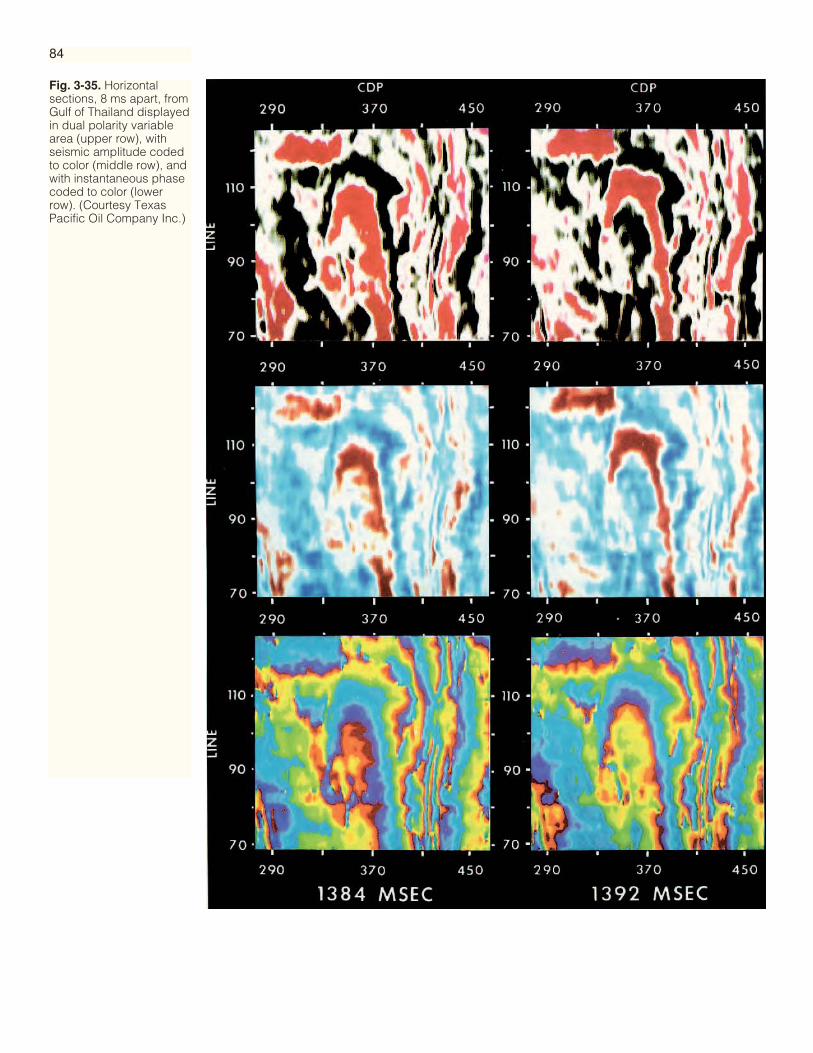
84

Fig. 3-35. Horizontalsections, 8 ms apart, fromGulf of Thailand displayedin dual polarity variablearea (upper row), withseismic amplitude codedto color (middle row), andwith instantaneous phasecoded to color (lowerrow). (Courtesy TexasPacific Oil Company Inc.)

85

86

In 3-D interpretation we studiously avoid drawing old-fashioned phantom hori-zons. Figure 3-33 shows the preferable alternative. We track a horizon above theobjective horizon and displace it down with a constant time shift. Then we estimatethe mistie between this and the desired horizon at several locations and interpolate amistie, or correction, map. By adding this to the displaced horizon map we shouldobtain something close to what is desired. We can then manually adjust as necessary,but the amount of manual work should be small compared with the traditional man-ual approach for the whole project.

Figure 3-34 illustrates a way of generating a confidence map to communicate tomanagers, engineers, clients, and others the confidence we have in the interpretedmaps we produce. Qualitative assessment of confidence, here using three levels, ismade occasionally based on data quality and whatever interpretation difficulties mayoccur. The resultant interpolated confidence map can be included with final maps forthe benefit of those who later use them.

With increasingly successful amplitude preservation in seismic processing, inter-preters are increasingly suffering from the limited optical dynamic range of conven-tional seismic displays. Too common are the variable area sections where some eventsof interest are heavily saturated and others have barely enough trace deflection to bevisible. This applies to all displays, vertical and horizontal, made with variable areatechniques. Horizontal sections, historically, were first made with variable area using

Fig. 3-36. Waveformdefinition using dualpolarity variable areasections. The troughs areshown as excursions tothe left; in practicesections are displayedwith the troughs rectifiedand hence swinging tothe right.

Advantages andDisadvantages of

Different Displays

87

one polarity only, normally peaks. This soon evolved into dual polarity variable areagiving equal weight to peaks and troughs (see Chapter 2). This is exemplified by theupper row of sections in Figure 3-35 and explained in detail by the diagram of Figure3-36.

Dual polarity variable area provides five clearly discernible amplitude levels. Thehighest amplitude peaks are saturated and appear as continuous black areas; themedium amplitude peaks do not coalesce and appear as discontinuous black areaswhich look gray; the lowest amplitudes are below the variable area bias level andappear white; the medium amplitude troughs appear pink; and the highest amplitudetroughs are continuous red areas.

If the detail in the seismic waveform provided by dual polarity variable area isinadequate, which is commonly the case today, then the increased dynamic range offull variable intensity color is required. The many ways of using color to interpretiveadvantage are discussed in Chapter 2. Gradational blue and red is a most usefulapplication; this is illustrated in the middle row of sections in Figure 3-35 andexplained in detail by the diagram of Figure 3-37. On such a display the interpretercan see the local amplitude maxima of a peak (or a trough) and draw a contour alongthe locus of those maxima, thus picking the crest of the seismic waveform.

A further option available to the structural interpreter is horizontal sections dis-played in phase, using instantaneous phase derived from the complex trace (Taner,Koehler and Sheriff, 1979). This approach is illustrated by the lower row of sections in

Fig. 3-37. Waveformdefinition using amplitudeand phase color sections.

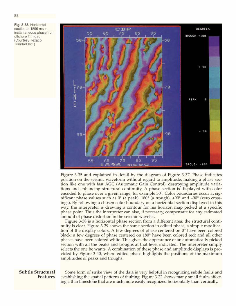
88

Figure 3-35 and explained in detail by the diagram of Figure 3-37. Phase indicatesposition on the seismic waveform without regard to amplitude, making a phase sec-tion like one with fast AGC (Automatic Gain Control), destroying amplitude varia-tions and enhancing structural continuity. A phase section is displayed with colorencoded to phase over a given range, for example 30°. Color boundaries occur at sig-nificant phase values such as 0° (a peak), 180° (a trough), +90° and –90° (zero cross-ings). By following a chosen color boundary on a horizontal section displayed in thisway, the interpreter is drawing a contour for his horizon map picked at a specificphase point. Thus the interpreter can also, if necessary, compensate for any estimatedamount of phase distortion in the seismic wavelet.

Figure 3-38 is a horizontal phase section from a different area; the structural conti-nuity is clear. Figure 3-39 shows the same section in edited phase, a simple modifica-tion of the display colors. A few degrees of phase centered on 0° have been coloredblack; a few degrees of phase centered on 180° have been colored red; and all otherphases have been colored white. This gives the appearance of an automatically pickedsection with all the peaks and troughs at that level indicated. The interpreter simplyselects the one he wants. A combination of these phase and amplitude displays is pro-vided by Figure 3-40, where edited phase highlights the positions of the maximumamplitudes of peaks and troughs.

Some form of strike view of the data is very helpful in recognizing subtle faults andestablishing the spatial patterns of faulting. Figure 3-22 shows many small faults affect-ing a thin limestone that are much more easily recognized horizontally than vertically.

Fig. 3-38. Horizontalsection at 1896 ms ininstantaneous phase fromoffshore Trinidad.(Courtesy TexacoTrinidad Inc.)

Subtle StructuralFeatures

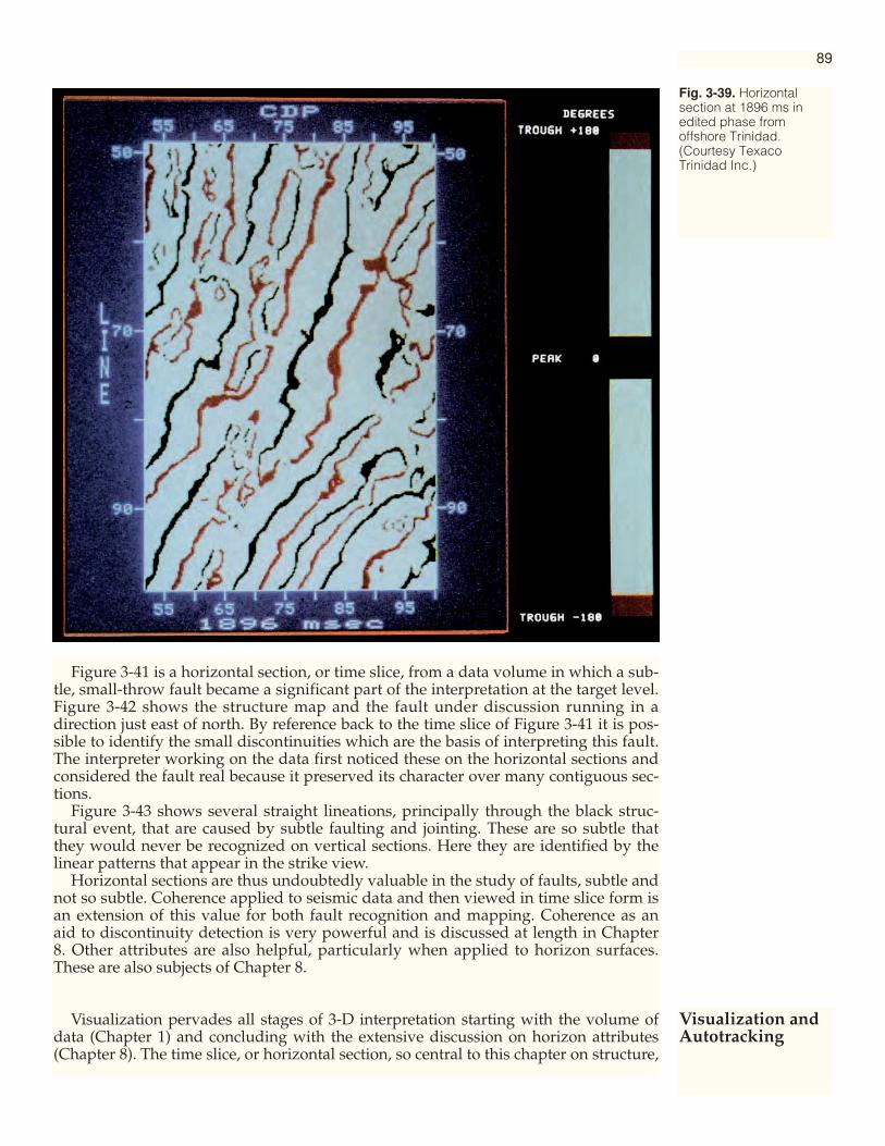
89

Figure 3-41 is a horizontal section, or time slice, from a data volume in which a sub-tle, small-throw fault became a significant part of the interpretation at the target level.Figure 3-42 shows the structure map and the fault under discussion running in adirection just east of north. By reference back to the time slice of Figure 3-41 it is pos-sible to identify the small discontinuities which are the basis of interpreting this fault.The interpreter working on the data first noticed these on the horizontal sections andconsidered the fault real because it preserved its character over many contiguous sec-tions.

Figure 3-43 shows several straight lineations, principally through the black struc-tural event, that are caused by subtle faulting and jointing. These are so subtle thatthey would never be recognized on vertical sections. Here they are identified by thelinear patterns that appear in the strike view.

Horizontal sections are thus undoubtedly valuable in the study of faults, subtle andnot so subtle. Coherence applied to seismic data and then viewed in time slice form isan extension of this value for both fault recognition and mapping. Coherence as anaid to discontinuity detection is very powerful and is discussed at length in Chapter8. Other attributes are also helpful, particularly when applied to horizon surfaces.These are also subjects of Chapter 8.

Visualization pervades all stages of 3-D interpretation starting with the volume ofdata (Chapter 1) and concluding with the extensive discussion on horizon attributes(Chapter 8). The time slice, or horizontal section, so central to this chapter on structure,

Fig. 3-39. Horizontalsection at 1896 ms inedited phase fromoffshore Trinidad.(Courtesy TexacoTrinidad Inc.)

Visualization andAutotracking

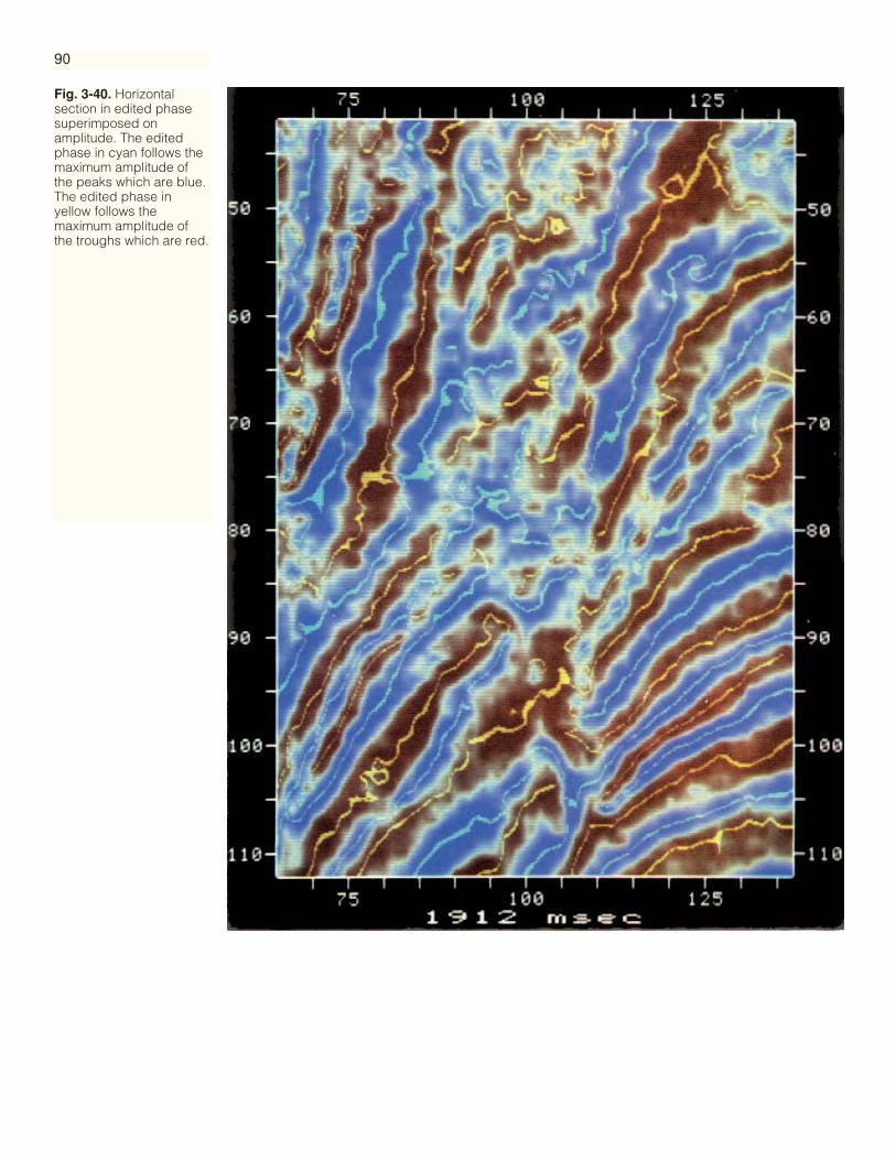
90

Fig. 3-40. Horizontalsection in edited phasesuperimposed onamplitude. The editedphase in cyan follows themaximum amplitude ofthe peaks which are blue.The edited phase inyellow follows themaximum amplitude ofthe troughs which are red.

91

Fig. 3-41. Horizontalsection at 2340 ms fromsouth Louisiana marshterrain. (CourtesyTexaco Inc.)

Fig. 3-42. Structuralcontour map showingsubtle fault identified onhorizontal section ofFigure 3-41. (CourtesyTexaco Inc.)

92

Fig. 3-43. Horizontalsection at 646 ms fromhigh resolution 3-D surveyat Ekofisk field in theNorth Sea. Note lineationsdue to faulting andjointing. (Courtesy PhillipsPetroleum CompanyNorway.)

93

is itself a major visualization aid and should be used as such. One vertical section andone horizontal section often provide an early visualization of the structure understudy.

Figure 3-44 is a time slice at 776 ms showing a distinctly circular feature about 3 kmin diameter and occurring at a depth of about 1000 m. It is a very striking view of animpact crater, or astrobleme, of Devonian age. The radial patterns in the centerstrongly suggest ejecta from the central uplift.

Once horizons and faults have been interpreted they can be visualized as surfaces(Figure 3-45). The relationship between the surfaces can then be studied to help invalidation of the interpretation and in placement of the wells to intersect multipleobjectives. Many new tools for visualization have recently been created and these arementioned in the Preface to the Fifth Edition.

The horizon surfaces above will have been produced using automatic spatial track-ing starting from seed, or control, points on vertical and horizontal sections. This

Fig. 3-44. Impact crater ofDevonian age seen ontime slice 776 ms from theUSA mid-continent. (Cour-tesy Texaco Explorationand Production Inc.)

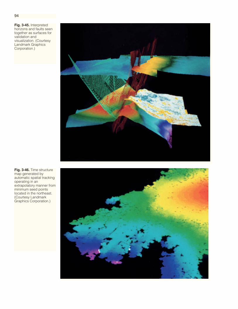
94

Fig. 3-45. Interpretedhorizons and faults seentogether as surfaces forvalidation andvisualization. (CourtesyLandmark GraphicsCorporation.)

Fig. 3-46. Time structuremap generated byautomatic spatial trackingoperating in anextrapolatory manner fromminimum seed pointslocated in the northeast.(Courtesy LandmarkGraphics Corporation.)

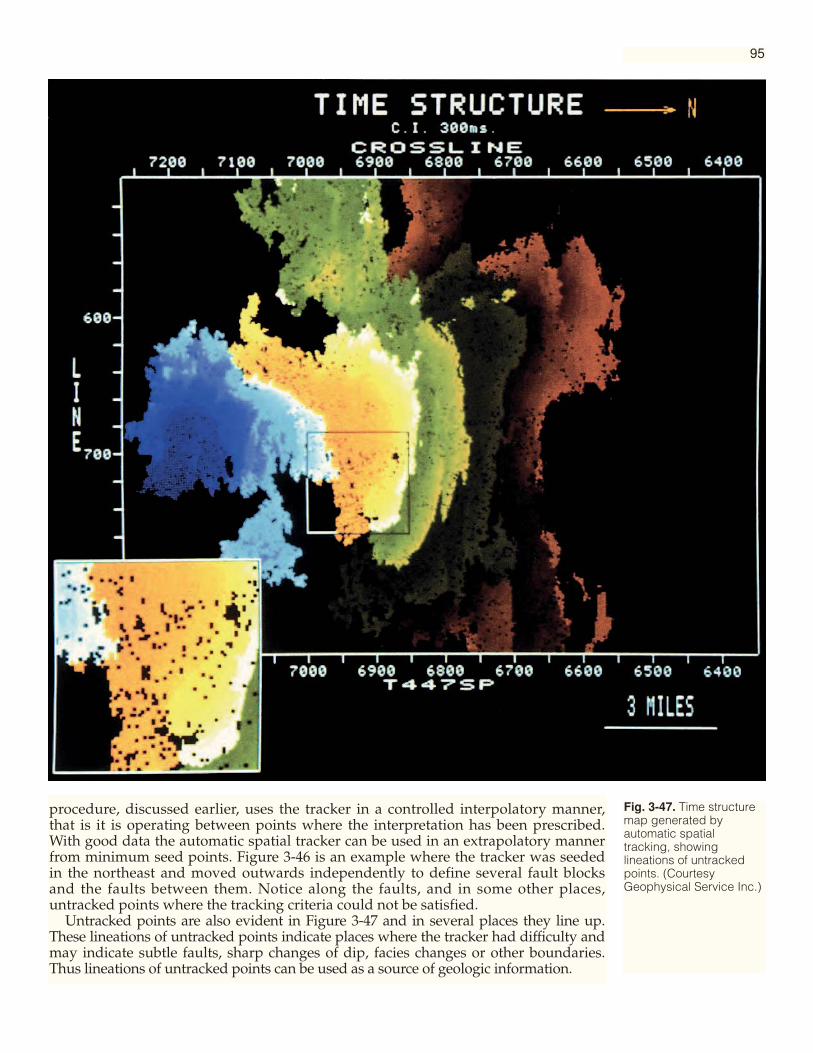
95

procedure, discussed earlier, uses the tracker in a controlled interpolatory manner,that is it is operating between points where the interpretation has been prescribed.With good data the automatic spatial tracker can be used in an extrapolatory mannerfrom minimum seed points. Figure 3-46 is an example where the tracker was seededin the northeast and moved outwards independently to define several fault blocksand the faults between them. Notice along the faults, and in some other places,untracked points where the tracking criteria could not be satisfied.

Untracked points are also evident in Figure 3-47 and in several places they line up.These lineations of untracked points indicate places where the tracker had difficulty andmay indicate subtle faults, sharp changes of dip, facies changes or other boundaries.Thus lineations of untracked points can be used as a source of geologic information.

Fig. 3-47. Time structuremap generated byautomatic spatialtracking, showinglineations of untrackedpoints. (CourtesyGeophysical Service Inc.)

96

Blake, B. A., J. B. Jennings, M. P. Curtis, and R. M. Phillipson, 1982, Three-dimensionalseismic data reveals the finer structural details of a piercement salt dome: OffshoreTechnology Conference Paper 4258, p. 403-406.

French, W. S., 1990, Practical seismic imaging: The Leading Edge, v. 9, no. 8, p. 13-20.Johnson, J. P., and M. R. Bone, 1980, Understanding field development history utiliz-

ing 3-D seismic: Offshore Technology Conference Paper 3849, p. 473-475.Stark, T. J., 1996, Surface slice generation and interpretation — a review: The Leading

Edge, v. 15, p. 818-819.Taner, M. T., F. Koehler, and R. E. Sheriff, 1979, Complex seismic trace analysis: Geo-

physics, v. 44, p. 1041-1063.

References

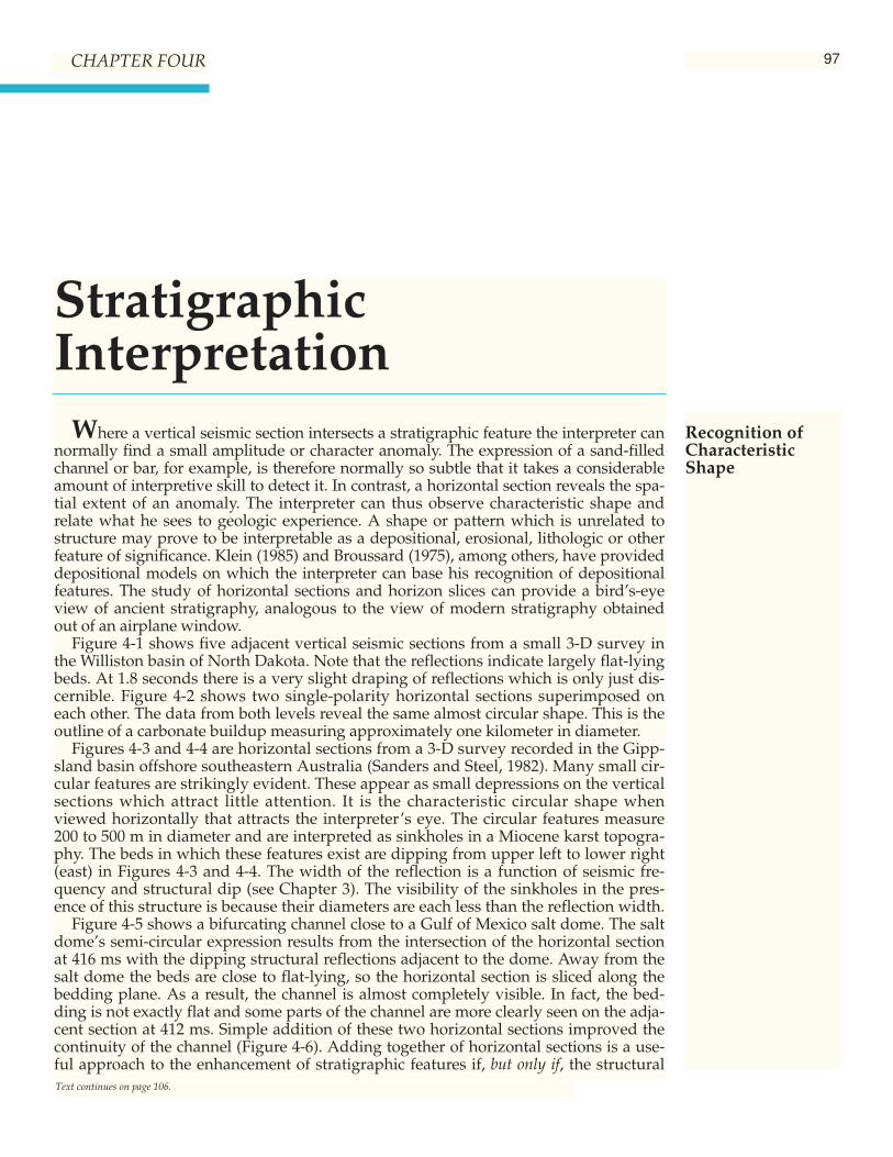
StratigraphicInterpretation

Where a vertical seismic section intersects a stratigraphic feature the interpreter cannormally find a small amplitude or character anomaly. The expression of a sand-filledchannel or bar, for example, is therefore normally so subtle that it takes a considerableamount of interpretive skill to detect it. In contrast, a horizontal section reveals the spa-tial extent of an anomaly. The interpreter can thus observe characteristic shape andrelate what he sees to geologic experience. A shape or pattern which is unrelated tostructure may prove to be interpretable as a depositional, erosional, lithologic or otherfeature of significance. Klein (1985) and Broussard (1975), among others, have provideddepositional models on which the interpreter can base his recognition of depositionalfeatures. The study of horizontal sections and horizon slices can provide a bird’s-eyeview of ancient stratigraphy, analogous to the view of modern stratigraphy obtainedout of an airplane window.

Figure 4-1 shows five adjacent vertical seismic sections from a small 3-D survey inthe Williston basin of North Dakota. Note that the reflections indicate largely flat-lyingbeds. At 1.8 seconds there is a very slight draping of reflections which is only just dis-cernible. Figure 4-2 shows two single-polarity horizontal sections superimposed oneach other. The data from both levels reveal the same almost circular shape. This is theoutline of a carbonate buildup measuring approximately one kilometer in diameter.

Figures 4-3 and 4-4 are horizontal sections from a 3-D survey recorded in the Gipp-sland basin offshore southeastern Australia (Sanders and Steel, 1982). Many small cir-cular features are strikingly evident. These appear as small depressions on the verticalsections which attract little attention. It is the characteristic circular shape whenviewed horizontally that attracts the interpreter’s eye. The circular features measure200 to 500 m in diameter and are interpreted as sinkholes in a Miocene karst topogra-phy. The beds in which these features exist are dipping from upper left to lower right(east) in Figures 4-3 and 4-4. The width of the reflection is a function of seismic fre-quency and structural dip (see Chapter 3). The visibility of the sinkholes in the pres-ence of this structure is because their diameters are each less than the reflection width.

Figure 4-5 shows a bifurcating channel close to a Gulf of Mexico salt dome. The saltdome’s semi-circular expression results from the intersection of the horizontal sectionat 416 ms with the dipping structural reflections adjacent to the dome. Away from thesalt dome the beds are close to flat-lying, so the horizontal section is sliced along thebedding plane. As a result, the channel is almost completely visible. In fact, the bed-ding is not exactly flat and some parts of the channel are more clearly seen on the adja-cent section at 412 ms. Simple addition of these two horizontal sections improved thecontinuity of the channel (Figure 4-6). Adding together of horizontal sections is a use-ful approach to the enhancement of stratigraphic features if, but only if, the structural

Recognition ofCharacteristicShape

97CHAPTER FOUR

Text continues on page 106.

Fig. 4-1. Five adjacentvertical sections from 3-Dsurvey in the Willistonbasin of North Dakota.(Courtesy GeophysicalService Inc.)

98

Fig. 4-2. Horizontalsections from 1812 and1828 ms from NorthDakota, each showingpositive amplitudes only.The approximatelycircular outline betweenthe black and the grayindicates the shape of acarbonate buildup.(Courtesy GeophysicalService Inc.)

99

Fig. 4-3. Horizontalsection at 820 ms from 3-D survey over Mackerelfield in offshoreGippsland basin,southeastern Australia.Circular objects areinterpreted as sinkholes inkarst topography.(Courtesy Esso AustraliaLtd.)

100

Fig. 4-4. Horizontalsection at 868 ms from 3-D survey over Mackerelfield in offshoreGippsland basin,southeastern Australia.Circular objects areinterpreted as sinkholes inkarst topography.(Courtesy Esso AustraliaLtd.)

101

Fig. 4-5. Horizontalsection at 416 ms from 3-D survey in the Gulf ofMexico. The bifurcatingchannel is seen close tothe edge of a salt dome.(Courtesy Chevron U.S.A.Inc.)

102

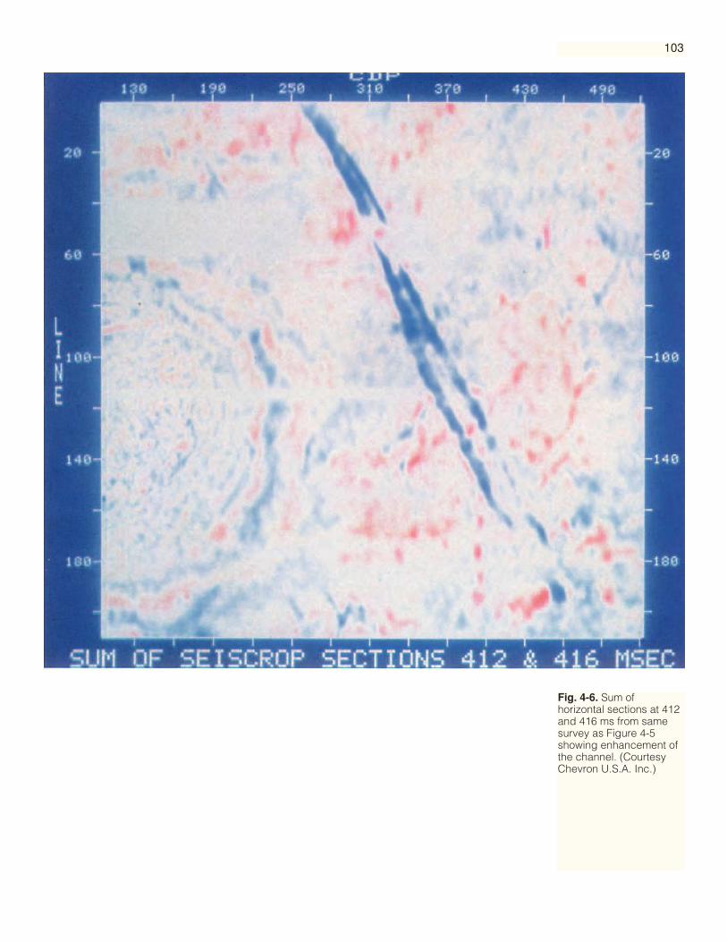
Fig. 4-6. Sum ofhorizontal sections at 412and 416 ms from samesurvey as Figure 4-5showing enhancement ofthe channel. (CourtesyChevron U.S.A. Inc.)

103

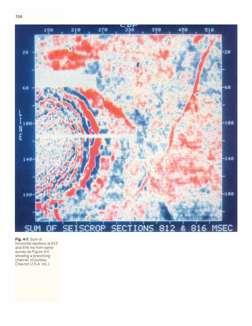
Fig. 4-7. Sum ofhorizontal sections at 812and 816 ms from samesurvey as Figure 4-5showing a branchingchannel. (CourtesyChevron U.S.A. Inc.)

104

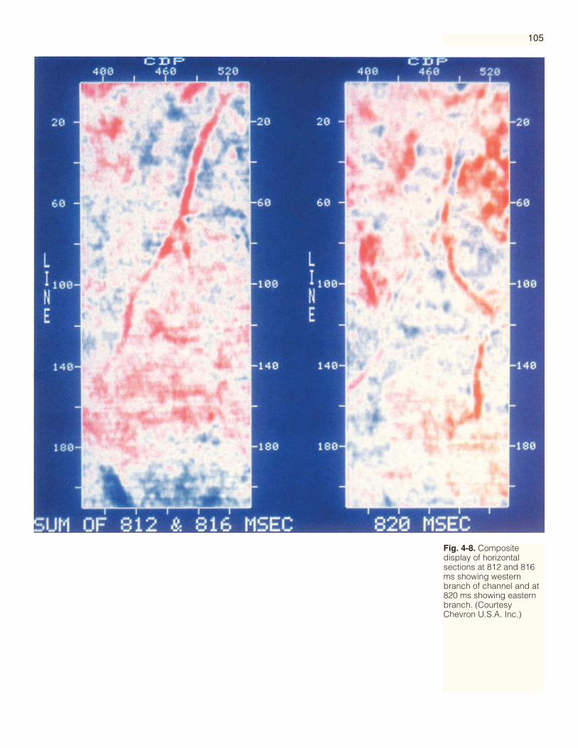
Fig. 4-8. Compositedisplay of horizontalsections at 812 and 816ms showing westernbranch of channel and at820 ms showing easternbranch. (CourtesyChevron U.S.A. Inc.)

105

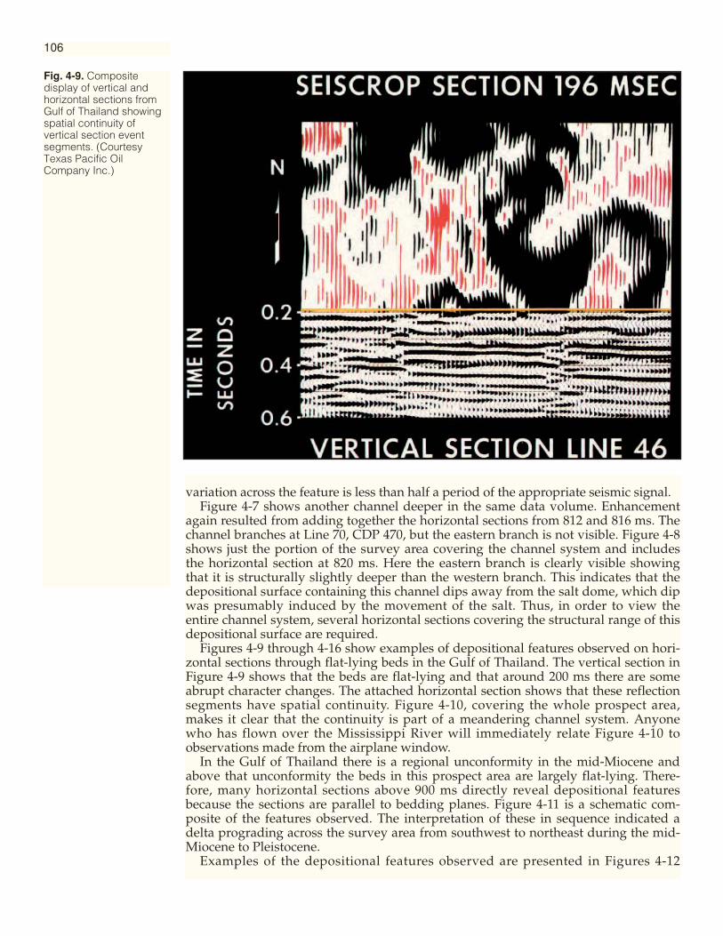
variation across the feature is less than half a period of the appropriate seismic signal.Figure 4-7 shows another channel deeper in the same data volume. Enhancement

again resulted from adding together the horizontal sections from 812 and 816 ms. Thechannel branches at Line 70, CDP 470, but the eastern branch is not visible. Figure 4-8shows just the portion of the survey area covering the channel system and includesthe horizontal section at 820 ms. Here the eastern branch is clearly visible showingthat it is structurally slightly deeper than the western branch. This indicates that thedepositional surface containing this channel dips away from the salt dome, which dipwas presumably induced by the movement of the salt. Thus, in order to view theentire channel system, several horizontal sections covering the structural range of thisdepositional surface are required.

Figures 4-9 through 4-16 show examples of depositional features observed on hori-zontal sections through flat-lying beds in the Gulf of Thailand. The vertical section inFigure 4-9 shows that the beds are flat-lying and that around 200 ms there are someabrupt character changes. The attached horizontal section shows that these reflectionsegments have spatial continuity. Figure 4-10, covering the whole prospect area,makes it clear that the continuity is part of a meandering channel system. Anyonewho has flown over the Mississippi River will immediately relate Figure 4-10 toobservations made from the airplane window.

In the Gulf of Thailand there is a regional unconformity in the mid-Miocene andabove that unconformity the beds in this prospect area are largely flat-lying. There-fore, many horizontal sections above 900 ms directly reveal depositional featuresbecause the sections are parallel to bedding planes. Figure 4-11 is a schematic com-posite of the features observed. The interpretation of these in sequence indicated adelta prograding across the survey area from southwest to northeast during the mid-Miocene to Pleistocene.

Examples of the depositional features observed are presented in Figures 4-12

Fig. 4-9. Compositedisplay of vertical andhorizontal sections fromGulf of Thailand showingspatial continuity ofvertical section eventsegments. (CourtesyTexas Pacific OilCompany Inc.)

106

through 4-16. Figure 4-12 shows in the upper center a delta front channel. Figure 4-13shows a large offshore bar trending northwest-southeast, transverse to the directionof delta progradation. Figure 4-14 shows two smaller bars, center and lower left, withthe same orientation. Figure 4-15 shows, in the upper right, a reworked bar; towardthe bottom are straight linear features suggestive of distributary channels. Figure 4-16shows many twisting channels, some of them very narrow.

Figure 4-17 shows part of the Mahakam delta in Indonesia. At this time (about18,000 years ago) deposition was clearly occurring in this part of the delta. Patternsare very similar to those visible in the present Mahakam delta (Figure 4-18). However,in another part of the ancient delta (Figure 4-19) erosion was occurring as evidencedby the dendritic patterns of canyons.

Figure 4-20 shows a shallow horizontal section from a part of the Gulf of Thailand

Fig. 4-10. Horizontalsection at 196 ms fromGulf of Thailand showingmeandering streamchannel. (Courtesy TexasPacific Oil Company Inc.)

107

Text continues on page 115.

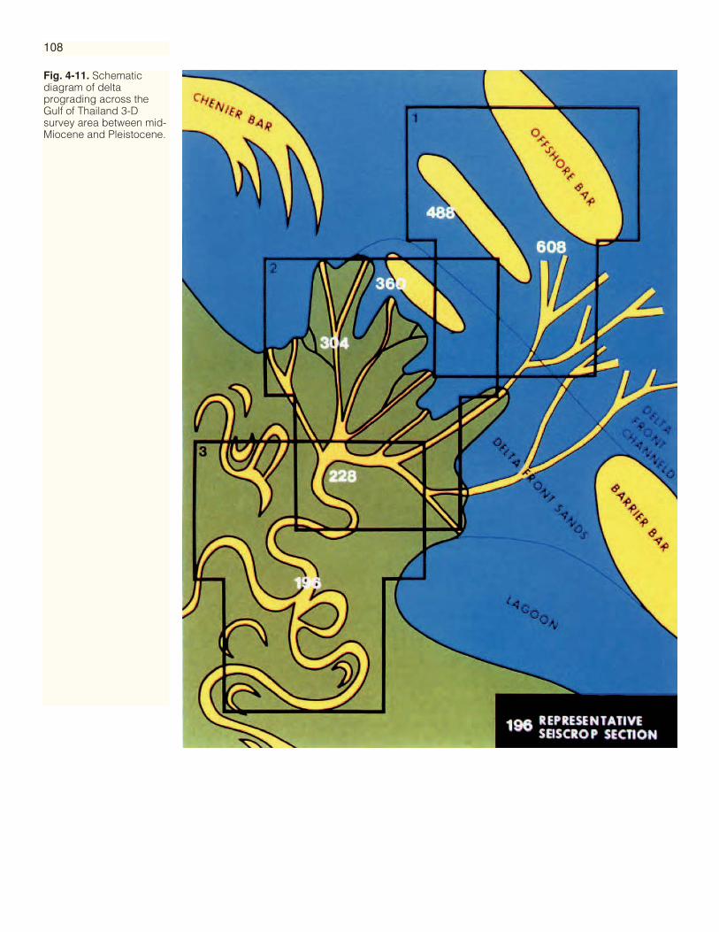
Fig. 4-11. Schematicdiagram of deltaprograding across theGulf of Thailand 3-Dsurvey area between mid-Miocene and Pleistocene.

108

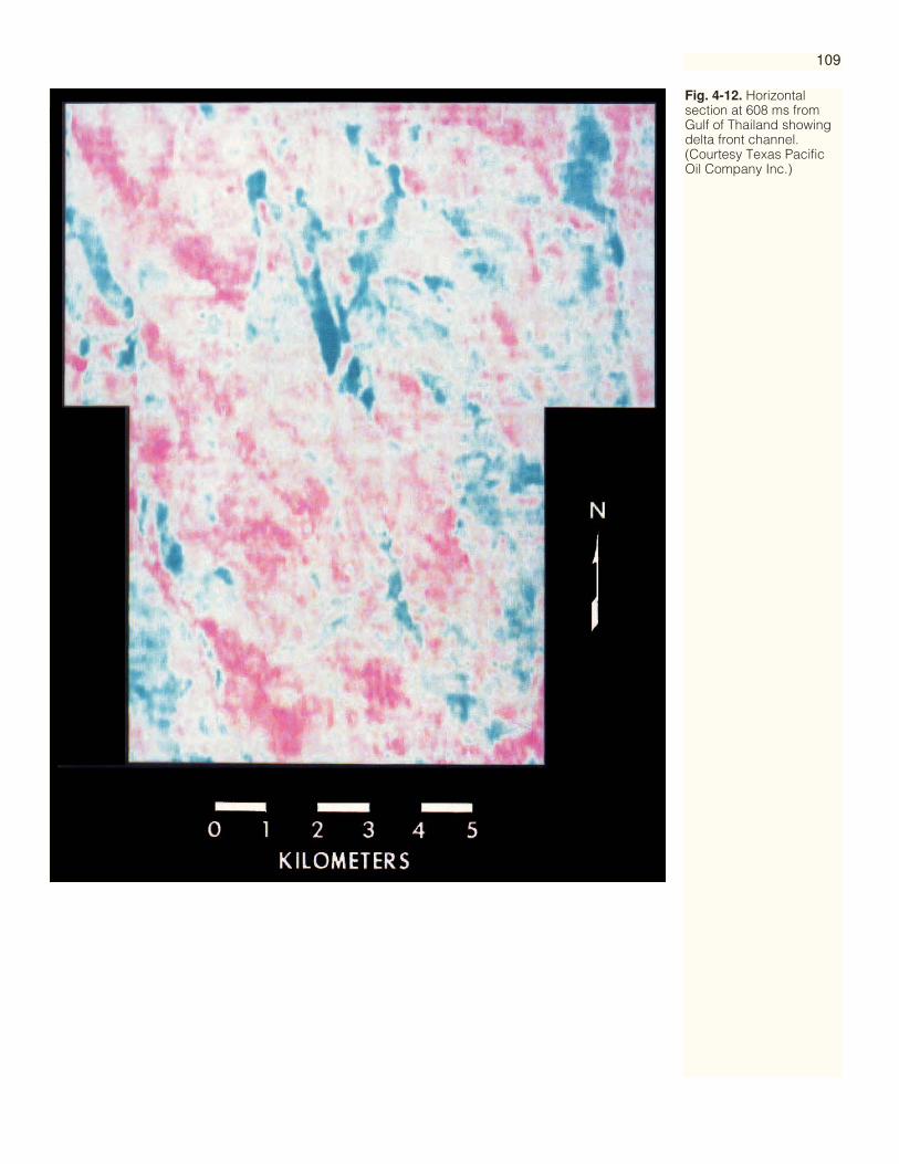
Fig. 4-12. Horizontalsection at 608 ms fromGulf of Thailand showingdelta front channel.(Courtesy Texas PacificOil Company Inc.)

109

Fig. 4-13. Horizontalsection at 488 ms fromGulf of Thailand showinglarge offshore sand bar.(Courtesy Texas PacificOil Company Inc.)

110

Fig. 4-14. Horizontalsection at 360 ms fromGulf of Thailand showingsmall sand bars.(Courtesy Texas PacificOil Company Inc.)

111

Fig. 4-15. Horizontalsection at 304 ms fromGulf of Thailand showinga reworked bar anddistributary channels.(Courtesy Texas PacificOil Company Inc.)

112

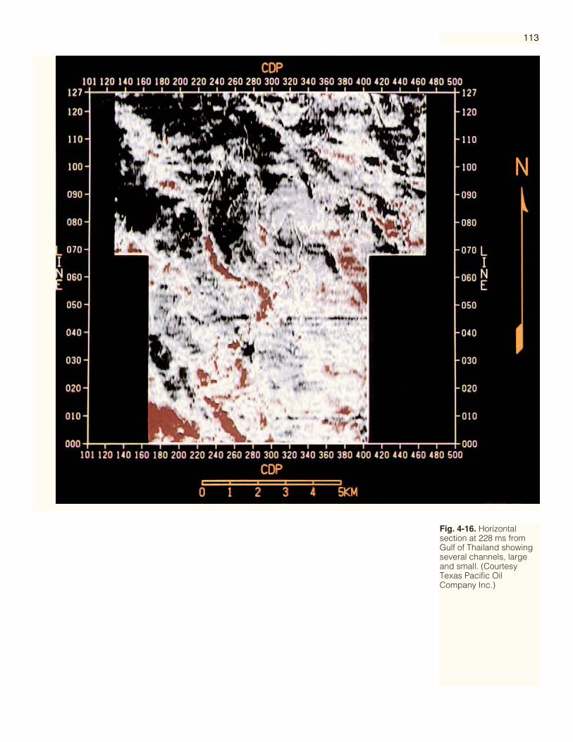
Fig. 4-16. Horizontalsection at 228 ms fromGulf of Thailand showingseveral channels, largeand small. (CourtesyTexas Pacific OilCompany Inc.)

113

Fig. 4-18. Satellite photo-graph of part of presentMahakam delta for com-parison with Figure 4-17.(Courtesy Total Indone-sie.)

114

Fig. 4-17. Horizontal sec-tion at 100 ms fromPeciko 3-D survey record-ed in the Mahakam deltaoffshore Kalimantan,Indonesia. The deltaicfeatures seen here areabout 18,000 years old.(Courtesy Total Indone-sie.)

115

Fig. 4-19. Horizontalsection at 104 ms fromNubi 3-D surveyrecorded in theMahakam delta off-shore Kalimantan,Indonesia. Note thedendritic patterns ofincised canyons. (Courtesy Total Indonesie.)

different from that discussed above; it covers a much larger area than other sectionsin this chapter, which is evidenced by the collage of eight panels. There is a plethoraof depositional features clearly visible. In the lowermost and uppermost parts of thefigure, channels cross each other. This is evidence that a horizontal section observes aslab of the subsurface of finite thickness (around a quarter of a wavelength) duringthe deposition of which, in this area, conditions changed significantly. On the rightcenter of Figure 4-20 a meandering channel is visible. Where this channel turns intothe center of the figure, it passes point bars inside the meander loops and crevassesplays outside them.

Figure 4-21 is a horizontal section from the Gulf of Mexico showing another clearlyvisible channel. The channel is fairly difficult to observe on the companion verticalsection of Figure 4-22. This demonstrates again the unique value of the strike perspec-tive in recognizing characteristic stratigraphic patterns.

Figure 4-23 shows the interpretation of several Miocene deltaic fans. They are visi-ble on one horizontal section because the structural dip is very gentle. Figure 4-24shows one deltaic fan from deeper within the same area. The single gray scale usedfor display of these two examples was beneficial for the overall fan morphologybecause much of the stratigraphic patterns were in low amplitudes (refer to the dis-cussion of color schemes in Chapter 2).

In general, stratigraphic features, after being deposited on a flat-lying surface, willbe bent and broken by later tectonic movements. Stratigraphy and structure thenbecome confused and the interpretive task comes in separating them. The structuremust be interpreted before stratigraphy can be appreciated.

Reconstituting aDepositionalSurface

Fig. 4-20. Shallowhorizontal section fromGulf of Thailand showingchannels, point bars andcrevasse splays.(Courtesy UnocalThailand Ltd.)

116

Fig. 4-21. Horizontalsection from MatagordaBlock 668, offshoreTexas, showing prominentchannel. It is a useful andinteresting challenge tolocate the channelintersection on the verticalsection of Figure 4-22.(Courtesy ARCO Oil andGas Company.)

Fig. 4-22. Vertical sectionfrom Matagorda Block668, offshore Texas.(Courtesy ARCO Oil andGas Company.)

117

Figure 4-25 illustrates schematically how a channel can be recognized and delineat-ed in the presence of structure. In this example the interpreter has horizontal sectionsat 4 ms intervals from 1240 to 1260 ms. The selected event at 1240 ms for the horizonunder study is traced to provide the contour as shown for 1240 ms. A high amplitudeanomaly is recognized and marked at the position of the green blob. This procedure isrepeated at 1244, 1248, 1252, 1256, and 1260 ms. At each of these levels the interpreterfound an amplitude anomaly; together these arranged themselves into the curvilinearfeature marked by the orange lines in Figure 4-25. This is manual amplitude mappingbut the interactive workstation gives us several tools to do this in an efficient way.

Figure 4-26 shows a vertical section interpreted on three horizons. The ShallowHorizon, marked in blue, was selected on the basis of both structural and stratigraph-ic objectives. Figure 4-27 shows the structural contour map of the Shallow Horizonresulting from a full-scale structural interpretation of all the 3-D data. The desire thenwas to slice through the data volume along this structurally interpreted horizon inorder to gather up all the seismic amplitudes associated with it. This is normallyaccomplished by the process of amplitude extraction, a menu-initiated search-and-gath-er operation on the interactive workstation. Alternatively, it is possible to flatten thedata volume on the Shallow Horizon, as structurally interpreted in Figure 4-27, andthen slice horizontally through the flattened volume at the level of the interpretedhorizon.

The resultant section is known as a horizon slice, horizon amplitude map, or hori-zon Seiscrop section, where the critical word is horizon. This type of section, follow-ing one horizon, must be along bedding planes or it loses its value for stratigraphic

118

Fig. 4-23. Horizontalsection at 936 ms fromMobile area, offshoreAlabama, showinginterpretation of numerousMiocene deltaic fans.(Courtesy Conoco Inc.and Digicon GeophysicalCorp.)

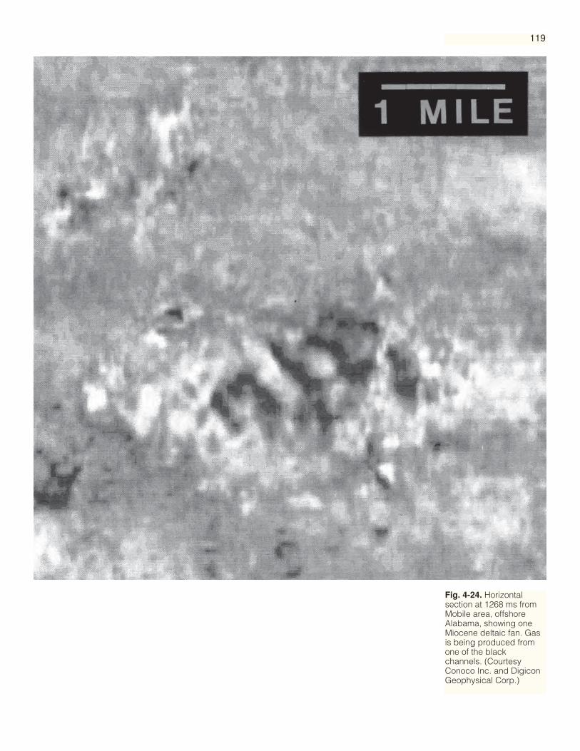
Fig. 4-24. Horizontalsection at 1268 ms fromMobile area, offshoreAlabama, showing oneMiocene deltaic fan. Gasis being produced fromone of the blackchannels. (CourtesyConoco Inc. and DigiconGeophysical Corp.)

119

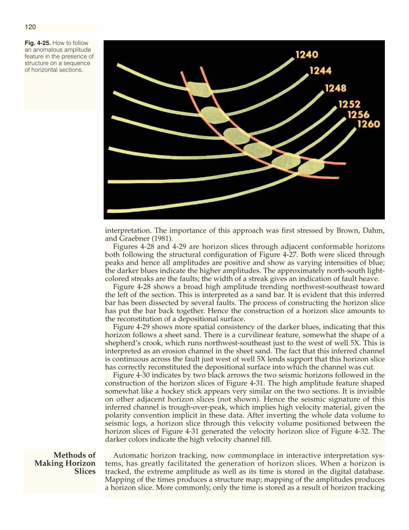
interpretation. The importance of this approach was first stressed by Brown, Dahm,and Graebner (1981).

Figures 4-28 and 4-29 are horizon slices through adjacent conformable horizonsboth following the structural configuration of Figure 4-27. Both were sliced throughpeaks and hence all amplitudes are positive and show as varying intensities of blue;the darker blues indicate the higher amplitudes. The approximately north-south light-colored streaks are the faults; the width of a streak gives an indication of fault heave.

Figure 4-28 shows a broad high amplitude trending northwest-southeast towardthe left of the section. This is interpreted as a sand bar. It is evident that this inferredbar has been dissected by several faults. The process of constructing the horizon slicehas put the bar back together. Hence the construction of a horizon slice amounts tothe reconstitution of a depositional surface.

Figure 4-29 shows more spatial consistency of the darker blues, indicating that thishorizon follows a sheet sand. There is a curvilinear feature, somewhat the shape of ashepherd’s crook, which runs northwest-southeast just to the west of well 5X. This isinterpreted as an erosion channel in the sheet sand. The fact that this inferred channelis continuous across the fault just west of well 5X lends support that this horizon slicehas correctly reconstituted the depositional surface into which the channel was cut.

Figure 4-30 indicates by two black arrows the two seismic horizons followed in theconstruction of the horizon slices of Figure 4-31. The high amplitude feature shapedsomewhat like a hockey stick appears very similar on the two sections. It is invisibleon other adjacent horizon slices (not shown). Hence the seismic signature of thisinferred channel is trough-over-peak, which implies high velocity material, given thepolarity convention implicit in these data. After inverting the whole data volume toseismic logs, a horizon slice through this velocity volume positioned between thehorizon slices of Figure 4-31 generated the velocity horizon slice of Figure 4-32. Thedarker colors indicate the high velocity channel fill.

Automatic horizon tracking, now commonplace in interactive interpretation sys-tems, has greatly facilitated the generation of horizon slices. When a horizon istracked, the extreme amplitude as well as its time is stored in the digital database.Mapping of the times produces a structure map; mapping of the amplitudes producesa horizon slice. More commonly, only the time is stored as a result of horizon tracking

Fig. 4-25. How to followan anomalous amplitudefeature in the presence ofstructure on a sequenceof horizontal sections.

120

Methods ofMaking Horizon

Slices

and later the amplitudes are extracted from the data. In addition, it is possible toextract the amplitudes not coincident with the tracked horizon but parallel to it andshifted by a chosen number of milliseconds.

Figure 4-33 shows two lines from a Gulf of Mexico 3-D prospect, where a horizon istracked one-and-a-half periods above a red blob considered to be of stratigraphicinterest. The structural continuity is better for the horizon being tracked than for theblob, so the structure was defined at this level and the horizon slice made parallel to itthrough the blob at a fixed time increment deeper.

The resulting horizon slice is shown in Figure 4-34 and the interpreter can readilyinfer the existence of another channel. The black horizontal lines indicate the posi-tions of the two vertical sections of Figure 4-33. The amplitude of the channel reflec-tion is greater to the northeast; a discussion of this relative to implied gas contentappears in Chapter 5.

A horizon slice is by definition a slice along a bedding plane, but the methods bywhich an interpreter may make such a slice are many and varied (Figure 4-35). If theslice is made at the tracking level, following automatic horizon tracking, the horizonslice is made up of truly crestal amplitudes and should thus be accurately along thebedding plane. However, if the structure is defined by tracking at one level where thecontinuity is clear but the slice is made parallel to that at another level, then the slic-ing and tracking levels must be sufficiently conformable for the horizon slice to ade-quately follow the bedding plane. This approach beneficially segregates the strati-graphic and structural components of an interpretation. Minor irregularities at thetracking level may not be paralleled at the slicing level, so spatial smoothing of thetracked times may be desirable before displacing the horizon down or up to the slic-ing level.

When a tracked horizon is displaced down by a constant time shift, the optionexists to snap the displaced horizon to the exact crestal amplitude of the new reflec-tion. Sometimes this will be the right course of action and sometimes it will be wrong.Figure 4-36 illustrates diagrammatically a situation where it would be wrong. Goodreflections exist at the sand/shale interface and the shale/limestone interface. How-ever, at the latter patches of porosity form the exploration objective and also intro-duce character changes along the limestone reflection. The shale is of uniform thick-ness. The structure is followed on the sand/shale reflection, which is stratigraphicallyuncomplicated, and displaced down by a constant time shift to the top of the lime-stone. The amplitudes are then extracted without snapping to yield a horizon slice onwhich the porosity should show as low amplitude patches. Snapping would move thehorizon down to the top of the unporous limestone and the low amplitude patcheswould be lost!

Slicing through a zone of poor reflection continuity (where tracking would havebeen impossible) parallel to a good reflection at the top or the base of the zone has inseveral cases yielded meaningful and interpretable stratigraphic patterns. Thisdemonstrates that data that may appear poor and uninterpretable on vertical sectionsmay in fact reveal significant stratigraphic information when viewed spatially overbedding plane surfaces. In the case of a poor continuity interval of nonuniform thick-ness it can be useful to track a reflection at the top and one at the base (Figure 4-37).Then the slice is made within that interval using a surface whose shape is based part-ly on the upper tracked surface and partly on the lower tracked surface, the propor-tions of each depending on where within the interval the slice is desired. This methodyields proportional slices.

After amplitude has been extracted on the objective horizon corrections are some-times required (Figure 4-35). Consider, for example, that a high amplitude bright spoton a deeper horizon slice is shadowed over part of its area by a shallower high ampli-tude anomaly. This is commonly referred to as transmission effect, and an example ofthis is discussed in Chapter 5. Some fraction of the amplitude extracted on the shal-lower horizon can be added to the amplitude on the deeper horizon to compensatefor the shadowing effect. The fraction to use must be established empirically but the

121

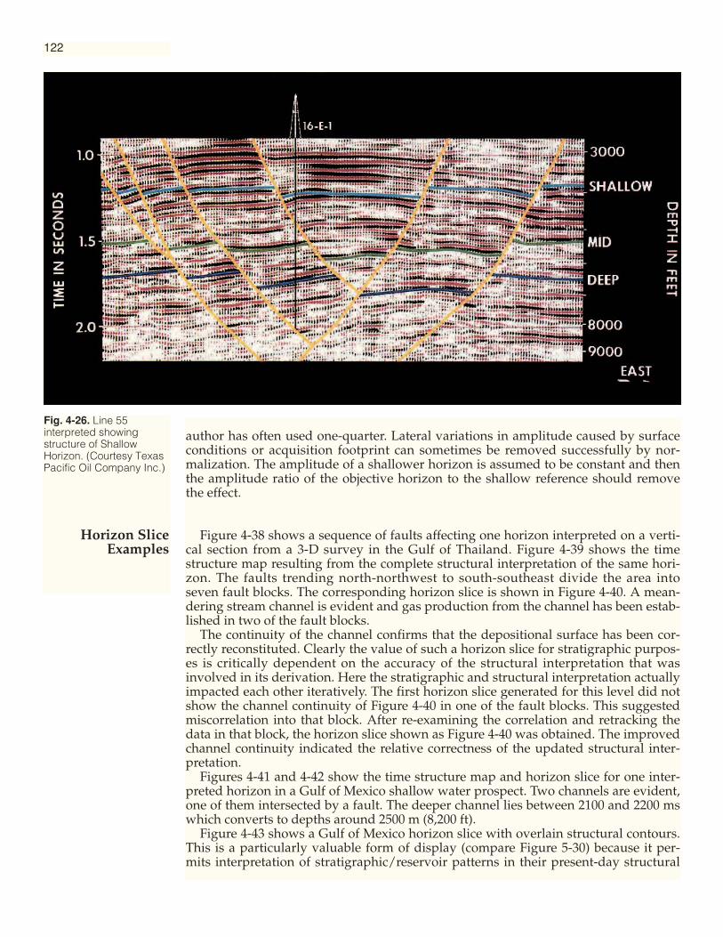
author has often used one-quarter. Lateral variations in amplitude caused by surfaceconditions or acquisition footprint can sometimes be removed successfully by nor-malization. The amplitude of a shallower horizon is assumed to be constant and thenthe amplitude ratio of the objective horizon to the shallow reference should removethe effect.

Figure 4-38 shows a sequence of faults affecting one horizon interpreted on a verti-cal section from a 3-D survey in the Gulf of Thailand. Figure 4-39 shows the timestructure map resulting from the complete structural interpretation of the same hori-zon. The faults trending north-northwest to south-southeast divide the area intoseven fault blocks. The corresponding horizon slice is shown in Figure 4-40. A mean-dering stream channel is evident and gas production from the channel has been estab-lished in two of the fault blocks.

The continuity of the channel confirms that the depositional surface has been cor-rectly reconstituted. Clearly the value of such a horizon slice for stratigraphic purpos-es is critically dependent on the accuracy of the structural interpretation that wasinvolved in its derivation. Here the stratigraphic and structural interpretation actuallyimpacted each other iteratively. The first horizon slice generated for this level did notshow the channel continuity of Figure 4-40 in one of the fault blocks. This suggestedmiscorrelation into that block. After re-examining the correlation and retracking thedata in that block, the horizon slice shown as Figure 4-40 was obtained. The improvedchannel continuity indicated the relative correctness of the updated structural inter-pretation.

Figures 4-41 and 4-42 show the time structure map and horizon slice for one inter-preted horizon in a Gulf of Mexico shallow water prospect. Two channels are evident,one of them intersected by a fault. The deeper channel lies between 2100 and 2200 mswhich converts to depths around 2500 m (8,200 ft).

Figure 4-43 shows a Gulf of Mexico horizon slice with overlain structural contours.This is a particularly valuable form of display (compare Figure 5-30) because it per-mits interpretation of stratigraphic/reservoir patterns in their present-day structural

Fig. 4-26. Line 55interpreted showingstructure of ShallowHorizon. (Courtesy TexasPacific Oil Company Inc.)

122

Horizon SliceExamples

Fig. 4-27. Time structuremap of Shallow Horizon.(Courtesy Texas PacificOil Company Inc.)

123

context. Here the high amplitudes (reds and oranges) are caused by gas in severalsand bodies. Note the sharp amplitude terminations toward the south (downdip),indicating the position of the gas-water contacts.

Figure 4-44 is an arbitrary line through three wells from a 3-D survey in southernCanada. The structure was defined at the Base Bow Island reflection. A slice parallelto this through the Glauconite zone yielded the horizon slice of Figure 4-45. Thisapproach was used in order to help distinguish stratigraphic variations from struc-tural variations at the objective level. Even then the stratigraphic patterns were notclearly apparent, but a further interpretation tied to well intersections yielded thesuperimposed stratigraphic descriptions.

Fig. 4-28. Horizon slice180 feet (60 m) belowShallow Horizon showingnorthwest- southeast-trending high amplitudeinterpreted as a sand bar.(Courtesy Texas PacificOil Company Inc.)

124

Figure 4-46 is a mosaic of amplitudes from 3-D and 2-D data from Argentina anddemonstrates the increased stratigraphic detail available from 3-D data (Gerster, 1995).Three 3-D surveys are shown; seven others exist in the immediate area.

Figure 4-47 is a horizon slice from offshore eastern Canada between 2.4 and 2.8 sec-onds showing many channels and their levees, an old shore line and an abandonedlake (Enachescu, 1993).

Figure 4-48 is a horizon slice from the Norwegian North Sea. The interesting fan-shaped feature is interpreted as a mass flow in the Danian (basal Tertiary) chalk.

The majority of the horizon slices presented in this chapter display seismic ampli-tude, and this also reflects the author’s usage. However, it is possible to make horizonslices in other attributes. Figure 4-32, for example, displays inversion velocity.

Fig. 4-29. Horizon slicethrough Shallow Horizonshowing a partly erodedsheet sand. (CourtesyTexas Pacific OilCompany Inc.)

125

Figure 4-49 shows a horizon slice from another Gulf of Mexico prospect. The ampli-tudes are in shades of blue and the time structure is superimposed as contour lineswith an interval of 100 ms. Several amplitude lineations are apparent. The ones run-ning approximately east-west are faults as evidenced by the displacement of the con-tours. The major lineation running north-northwest–south-southeast is apparentlyunrelated to the faulting. It is interpreted as the truncation of a sand dipping up fromthe east. It is probably a depositional edge but the erosional truncation of a sand at anunconformity would show in exactly the same manner. It is this lineation on the hori-zon slice which caught the interpreter’s eye and thus begged for an explanation.

An excellent example of the variation in reflection character and amplitude acrossan angular unconformity comes from the Lisburne 3-D survey. The following

UnconformityHorizon Slices

Text continues on page 134

Fig. 4-30. A portion of Line 55 through the central graben ofthe 3-D prospect. (Courtesy Texas Pacific Oil Company Inc.)

Fig. 4-31. Horizon slices through the two events marked with black arrows onFigure 4-30. The curvilinear features are interpreted as the reflections from the topand base of a channel. (Courtesy Texas Pacific Oil Company Inc.)

126

Fig. 4-32. Horizon slice invelocity positionedbetween the sections ofFigure 4-31 and showingthe extent of the highvelocity channel fill.(Courtesy Texas PacificOil Company Inc.)

127

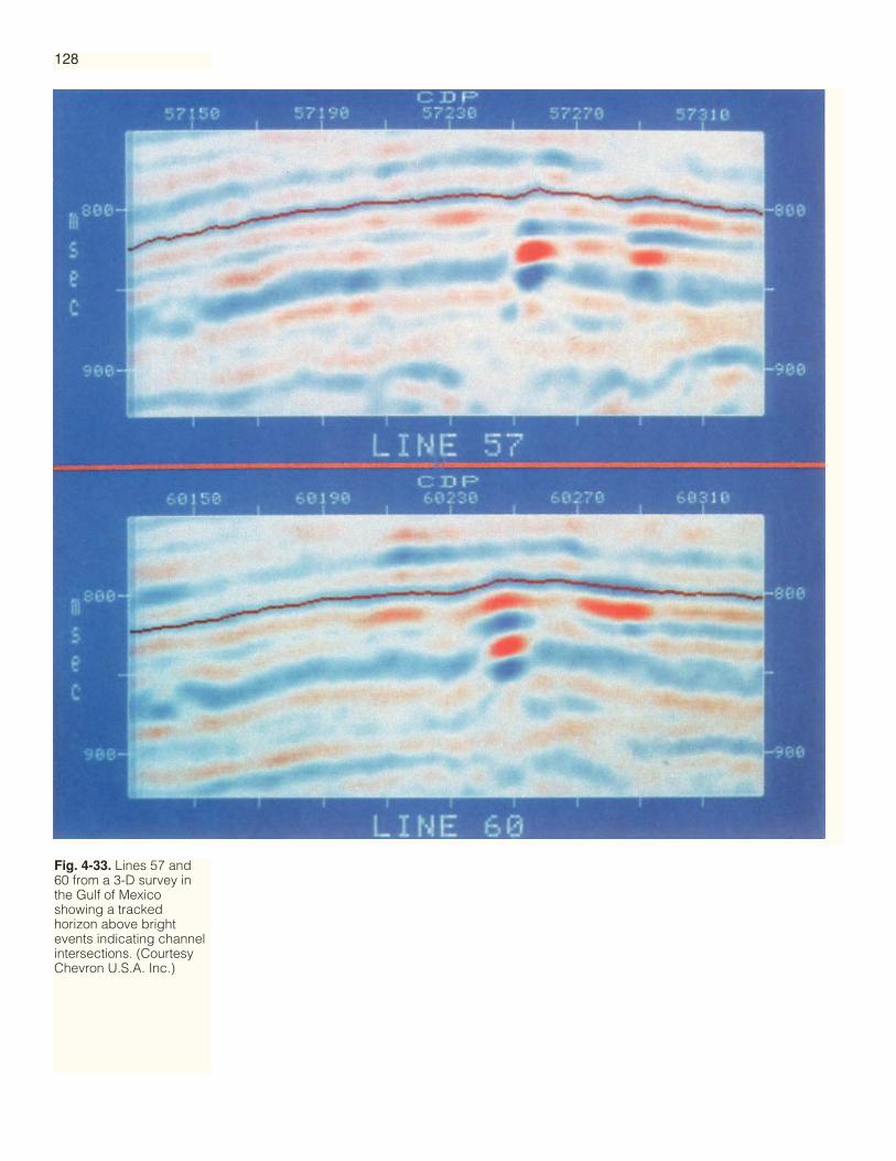
Fig. 4-33. Lines 57 and60 from a 3-D survey inthe Gulf of Mexicoshowing a trackedhorizon above brightevents indicating channelintersections. (CourtesyChevron U.S.A. Inc.)

128

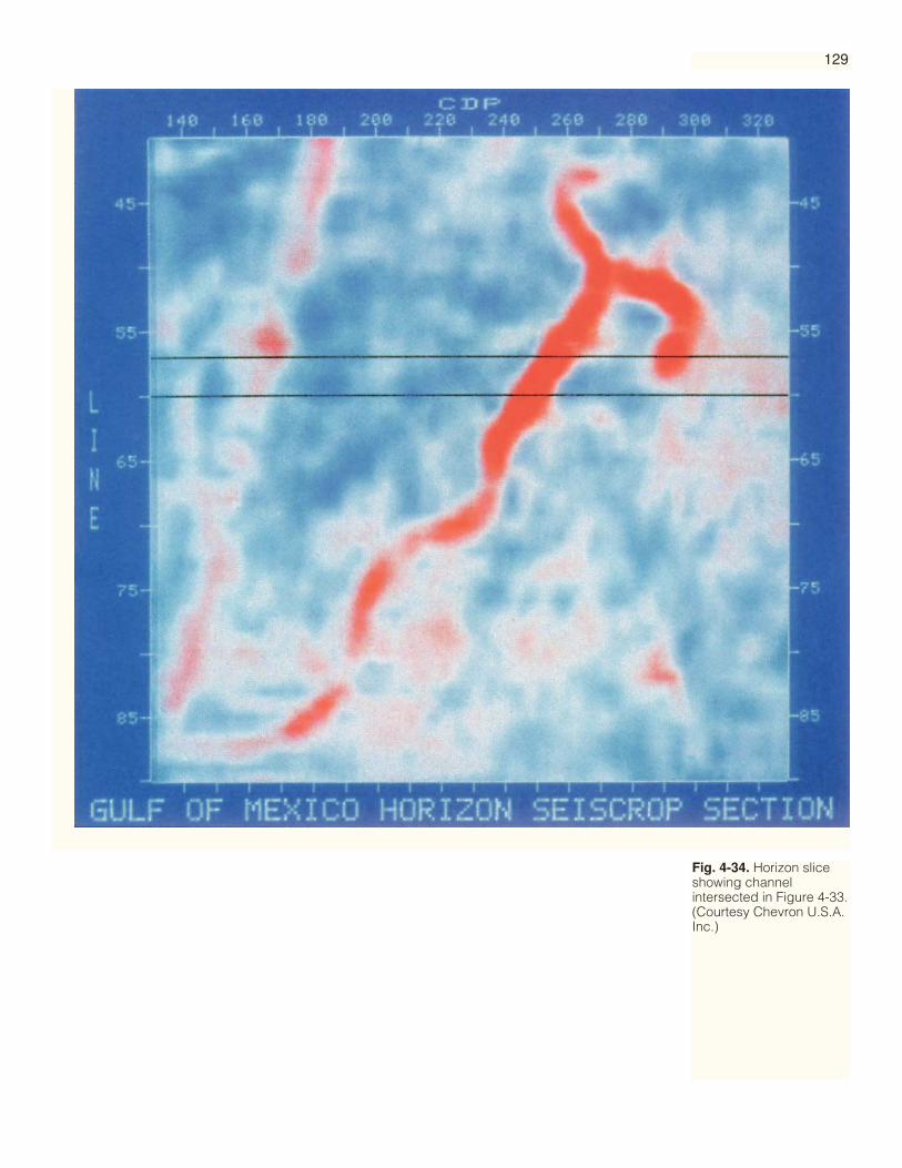
Fig. 4-34. Horizon sliceshowing channelintersected in Figure 4-33.(Courtesy Chevron U.S.A.Inc.)

129

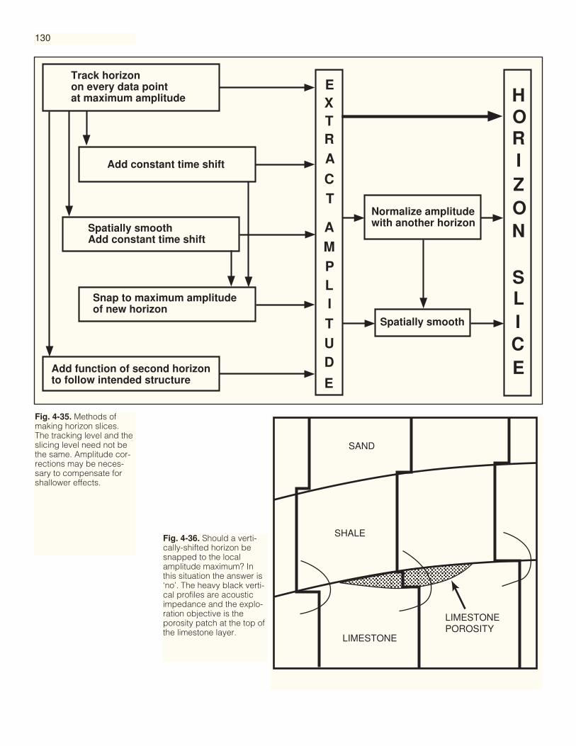
Fig. 4-35. Methods ofmaking horizon slices.The tracking level and theslicing level need not bethe same. Amplitude cor-rections may be neces-sary to compensate forshallower effects.

Fig. 4-36. Should a verti-cally-shifted horizon besnapped to the localamplitude maximum? Inthis situation the answer is‘no’. The heavy black verti-cal profiles are acousticimpedance and the explo-ration objective is theporosity patch at the top ofthe limestone layer.

130

Track horizonon every data pointat maximum amplitude

Add constant time shift

Spatially smoothAdd constant time shift

Snap to maximum amplitudeof new horizon

Add function of second horizonto follow intended structure

EXTRA

CT

AMPLITUD

E

HORIZON

SLICE

Spatially smooth

Normalize amplitudewith another horizon

������������������������������

SAND

SHALE

LIMESTONE

LIMESTONEPOROSITY

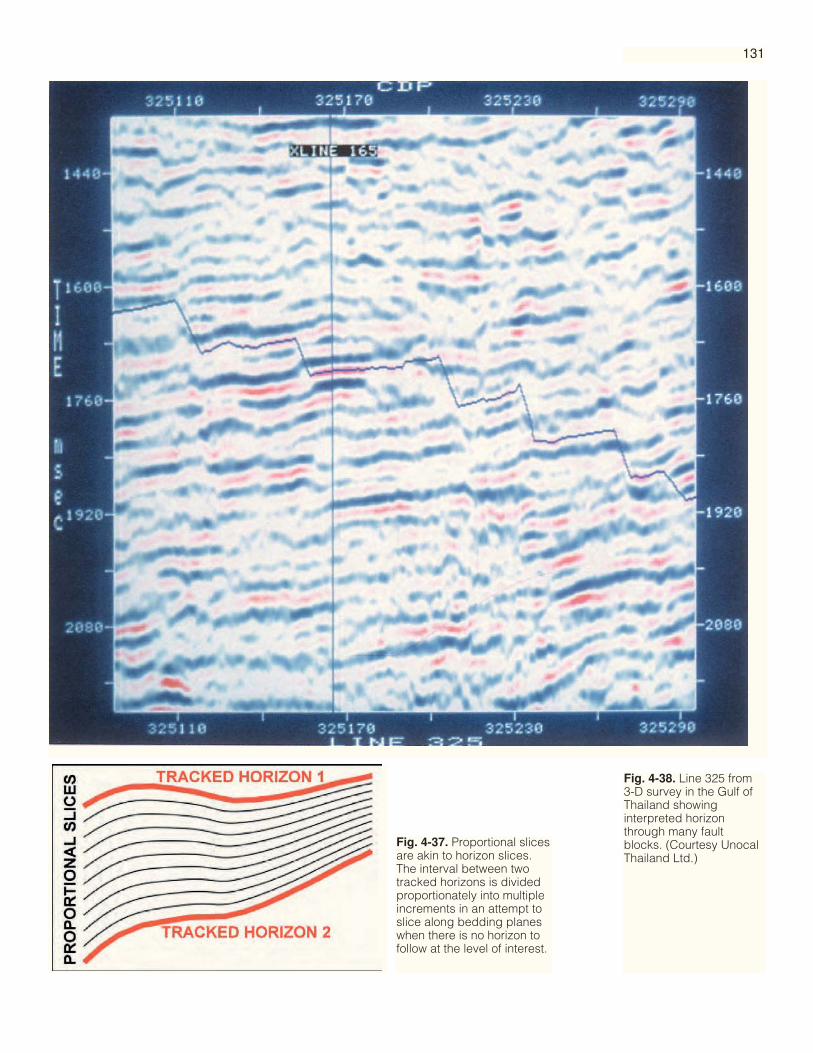
Fig. 4-38. Line 325 from3-D survey in the Gulf ofThailand showinginterpreted horizonthrough many faultblocks. (Courtesy UnocalThailand Ltd.)

131

Fig. 4-37. Proportional slicesare akin to horizon slices.The interval between twotracked horizons is dividedproportionately into multipleincrements in an attempt toslice along bedding planeswhen there is no horizon tofollow at the level of interest.

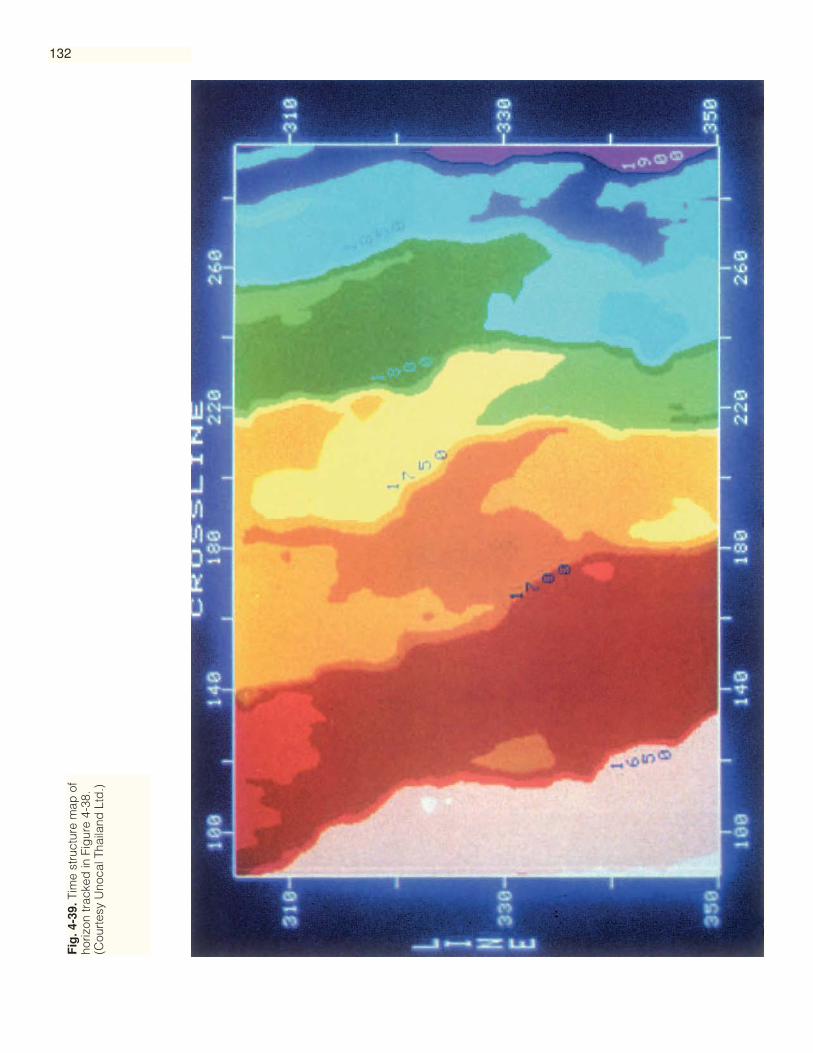
Fig

. 4-3

9.Ti

me

stru

ctur

e m

ap o

fho

rizon

trac

ked

in F

igur

e 4-

38.

(Cou

rtes

y U

noca

l Tha

iland

Ltd

.)

132

133

Fig

. 4-4

0.H

oriz

on s

lice

show

ing

sp

atia

l dis

trib

utio

nof

am

plit

ude

over

the

horiz

on m

app

ed in

Fig

ure

4-39

. Gas

pro

duc

tion

has

bee

n es

tab

lishe

d in

the

mea

nder

ing

cha

nnel

.(C

ourt

esy

Uno

cal T

haila

ndLt

d.)

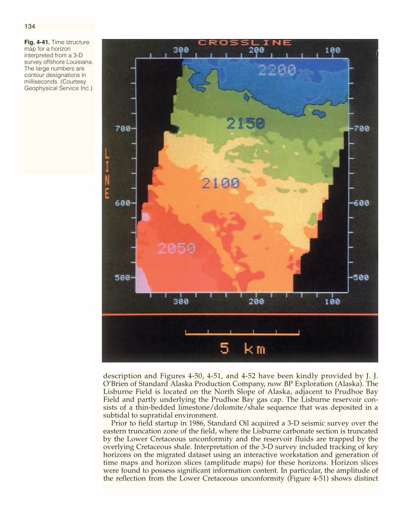
134

description and Figures 4-50, 4-51, and 4-52 have been kindly provided by J. J.O’Brien of Standard Alaska Production Company, now BP Exploration (Alaska). TheLisburne Field is located on the North Slope of Alaska, adjacent to Prudhoe BayField and partly underlying the Prudhoe Bay gas cap. The Lisburne reservoir con-sists of a thin-bedded limestone/dolomite/shale sequence that was deposited in asubtidal to supratidal environment.

Prior to field startup in 1986, Standard Oil acquired a 3-D seismic survey over theeastern truncation zone of the field, where the Lisburne carbonate section is truncatedby the Lower Cretaceous unconformity and the reservoir fluids are trapped by theoverlying Cretaceous shale. Interpretation of the 3-D survey included tracking of keyhorizons on the migrated dataset using an interactive workstation and generation oftime maps and horizon slices (amplitude maps) for these horizons. Horizon sliceswere found to possess significant information content. In particular, the amplitude ofthe reflection from the Lower Cretaceous unconformity (Figure 4-51) shows distinct

Fig. 4-41. Time structuremap for a horizoninterpreted from a 3-Dsurvey offshore Louisiana.The large numbers arecontour designations inmilliseconds. (CourtesyGeophysical Service Inc.)

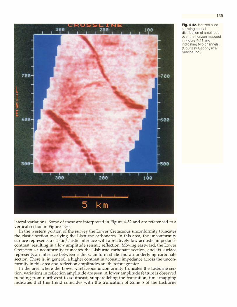
135

Fig. 4-42. Horizon sliceshowing spatialdistribution of amplitudeover the horizon mappedin Figure 4-41 andindicating two channels.(Courtesy GeophysicalService Inc.)

lateral variations. Some of these are interpreted in Figure 4-52 and are referenced to avertical section in Figure 4-50.

In the western portion of the survey the Lower Cretaceous unconformity truncatesthe clastic section overlying the Lisburne carbonates. In this area, the unconformitysurface represents a clastic/clastic interface with a relatively low acoustic impedancecontrast, resulting in a low amplitude seismic reflection. Moving eastward, the LowerCretaceous unconformity truncates the Lisburne carbonate section, and its surfacerepresents an interface between a thick, uniform shale and an underlying carbonatesection. There is, in general, a higher contrast in acoustic impedance across the uncon-formity in this area and reflection amplitudes are therefore greater.

In the area where the Lower Cretaceous unconformity truncates the Lisburne sec-tion, variations in reflection amplitude are seen. A lower amplitude feature is observedtrending from northwest to southeast, subparalleling the truncation; time mappingindicates that this trend coincides with the truncation of Zone 5 of the Lisburne

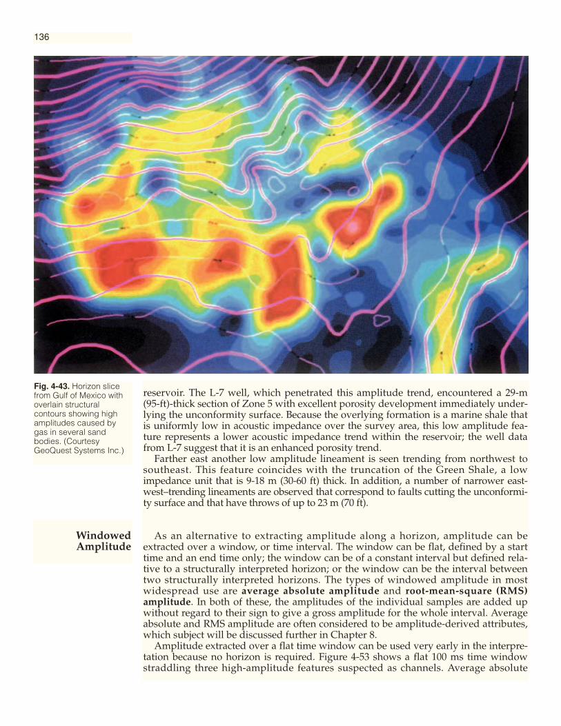
136

Fig. 4-43. Horizon slicefrom Gulf of Mexico withoverlain structuralcontours showing highamplitudes caused bygas in several sandbodies. (CourtesyGeoQuest Systems Inc.)

reservoir. The L-7 well, which penetrated this amplitude trend, encountered a 29-m(95-ft)-thick section of Zone 5 with excellent porosity development immediately under-lying the unconformity surface. Because the overlying formation is a marine shale thatis uniformly low in acoustic impedance over the survey area, this low amplitude fea-ture represents a lower acoustic impedance trend within the reservoir; the well datafrom L-7 suggest that it is an enhanced porosity trend.

Farther east another low amplitude lineament is seen trending from northwest tosoutheast. This feature coincides with the truncation of the Green Shale, a lowimpedance unit that is 9-18 m (30-60 ft) thick. In addition, a number of narrower east-west–trending lineaments are observed that correspond to faults cutting the unconformi-ty surface and that have throws of up to 23 m (70 ft).

As an alternative to extracting amplitude along a horizon, amplitude can beextracted over a window, or time interval. The window can be flat, defined by a starttime and an end time only; the window can be of a constant interval but defined rela-tive to a structurally interpreted horizon; or the window can be the interval betweentwo structurally interpreted horizons. The types of windowed amplitude in mostwidespread use are average absolute amplitude and root-mean-square (RMS)amplitude. In both of these, the amplitudes of the individual samples are added upwithout regard to their sign to give a gross amplitude for the whole interval. Averageabsolute and RMS amplitude are often considered to be amplitude-derived attributes,which subject will be discussed further in Chapter 8.

Amplitude extracted over a flat time window can be used very early in the interpre-tation because no horizon is required. Figure 4-53 shows a flat 100 ms time windowstraddling three high-amplitude features suspected as channels. Average absolute

WindowedAmplitude

Fig. 4-44. Arbitrary linejoining three wells inRetlaw prospect, southernAlberta, showing BaseBow Island reflection (thetracking level) andGlauconite Zone (theslicing level). (CourtesyGeophysical Service Inc.)

Fig. 4-45. Horizon slicethrough Glauconite Zone(near Top Mississippian)showing interpretation ofdepositional features.(Courtesy GeophysicalService Inc.)

137

138

Fig. 4-46. Distributionof Avile sand in part ofthe Neuquen basin,Argentina. Note theelongated eoliandunes. Horizon slicesfrom three 3-D surveysare compared withamplitude mappingfrom 2-D data. (Cour-tesy YPF S.A.)

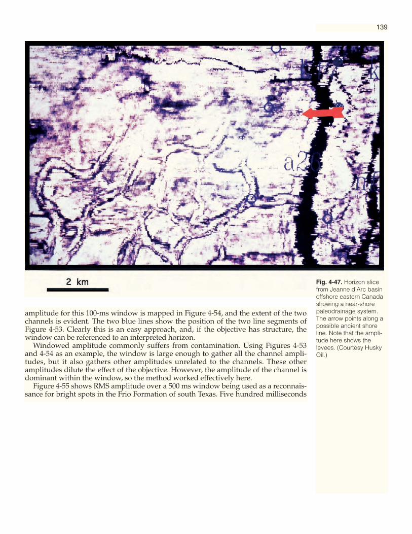
139

amplitude for this 100-ms window is mapped in Figure 4-54, and the extent of the twochannels is evident. The two blue lines show the position of the two line segments ofFigure 4-53. Clearly this is an easy approach, and, if the objective has structure, thewindow can be referenced to an interpreted horizon.

Windowed amplitude commonly suffers from contamination. Using Figures 4-53and 4-54 as an example, the window is large enough to gather all the channel ampli-tudes, but it also gathers other amplitudes unrelated to the channels. These otheramplitudes dilute the effect of the objective. However, the amplitude of the channel isdominant within the window, so the method worked effectively here.

Figure 4-55 shows RMS amplitude over a 500 ms window being used as a reconnais-sance for bright spots in the Frio Formation of south Texas. Five hundred milliseconds

Fig. 4-47. Horizon slicefrom Jeanne d’Arc basinoffshore eastern Canadashowing a near-shorepaleodrainage system.The arrow points along apossible ancient shoreline. Note that the ampli-tude here shows thelevees. (Courtesy HuskyOil.)

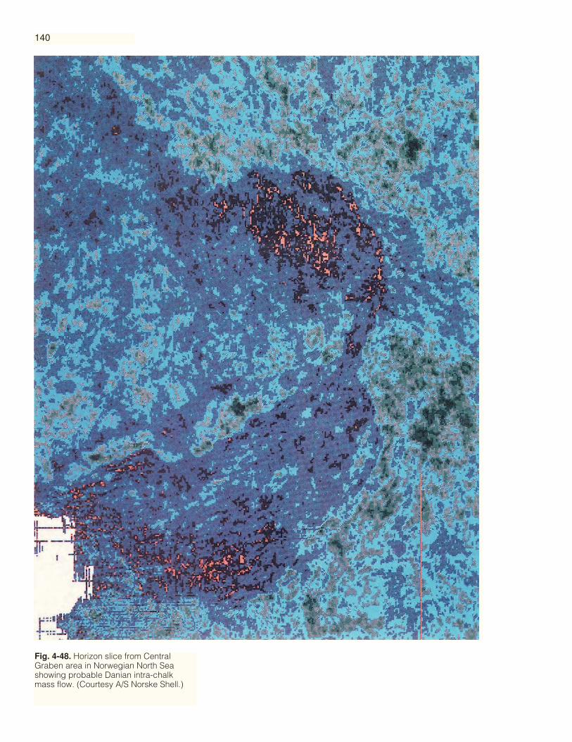
Fig. 4-48. Horizon slice from CentralGraben area in Norwegian North Seashowing probable Danian intra-chalkmass flow. (Courtesy A/S Norske Shell.)

140

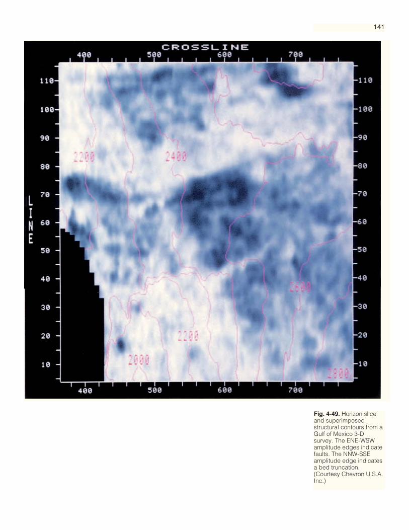
Fig. 4-49. Horizon sliceand superimposedstructural contours from aGulf of Mexico 3-Dsurvey. The ENE-WSWamplitude edges indicatefaults. The NNW-SSEamplitude edge indicatesa bed truncation.(Courtesy Chevron U.S.A.Inc.)

141

Fig

. 4-5

0.V

ertic

al s

ectio

n fr

omLi

sbur

ne 3

-D s

urve

y, N

orth

Slo

pe

of A

lask

a, s

how

ing

Low

er C

reta

ceou

sun

conf

orm

ity. (

Cou

rtes

yS

tand

ard

Ala

ska

Pro

duc

tion

Com

pan

y)

142

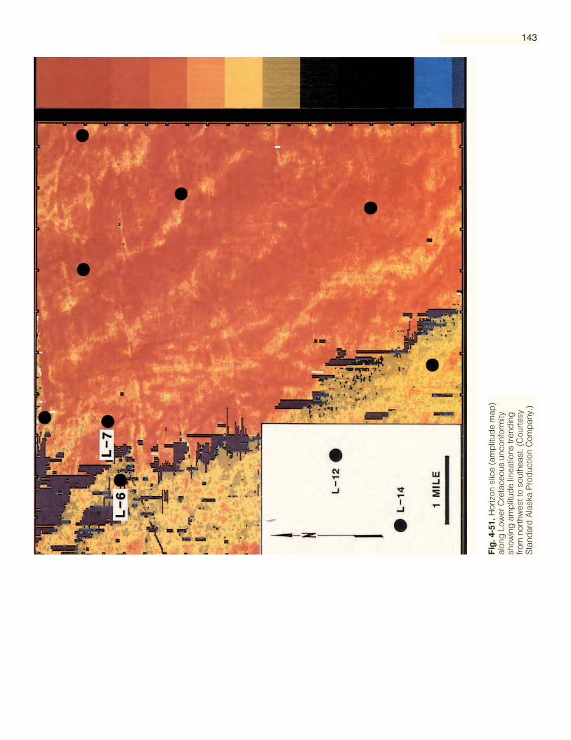
Fig

. 4-5

1.H

oriz

on s

lice

(am

plit

ude

map

)al

ong

Low

er C

reta

ceou

s un

conf

orm

itysh

owin

g a

mp

litud

e lin

eatio

ns tr

end

ing

from

nor

thw

est t

o so

uthe

ast.

(Cou

rtes

yS

tand

ard

Ala

ska

Pro

duc

tion

Com

pan

y.)

143

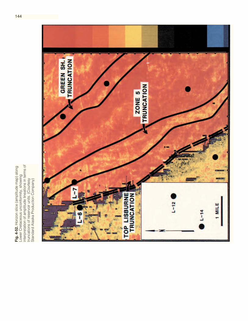
144F

ig. 4

-52.

Hor

izon

slic

e (a

mp

litud

e m

ap)

alon

gLo

wer

Cre

tace

ous

unco

nfor

mity

, sho

win

gin

terp

reta

tion

of a

mp

litud

e lin

eatio

ns in

term

s of

trun

catio

ns o

f res

ervo

ir un

its. (

Cou

rtes

yS

tand

ard

Ala

ska

Pro

duc

tion

Com

pan

y)

145

Fig. 4-53. Vertical seismic section from NorthSea showing 100-ms time window enclosinghigh-amplitude channel reflections. (CourtesyLandmark UK, Phillips UK and WesternGeophysical Corporation.)

Fig. 4-54. Averageabsolute amplitudecomputed over timewindow indicated inFigure 4-53. Notedefinition of channel.(Courtesy Landmark UK,Phillips UK and WesternGeophysicalCorporation.)

146

Fig

. 4-5

5. R

MS

am

plit

ude

from

a 5

00-m

s w

ind

ow s

pan

ning

Frio

For

mat

ion

brig

ht s

pot

s in

sou

th T

exas

. The

red

pat

ches

of

accu

mul

ated

hig

h am

plit

ude

can

be

seen

in r

elat

ion

to th

ew

ell p

enet

ratio

ns s

how

n in

yel

low

. (C

ourt

esy

Ed

ge

Pet

role

um.)

147

Fig

. 4-5

6. T

op B

ald

er

Form

atio

n am

plit

ude

map

fr

om m

ultip

le 3

-D s

urve

ys c

over

ing

55

00 s

q k

m o

f the

Far

oe B

asin

wes

t of

She

tland

in U

.K. w

ater

s. T

he c

olor

s sh

ow

RM

S a

mp

litud

e ov

er a

50-

ms

win

dow

sur

roun

din

g

the

Top

Bal

der

ref

lect

ion,

with

red

ind

icat

ing

hig

h am

plit

ude

and

blu

e in

dic

atin

g lo

w a

mp

litud

e. (

Cou

rtes

y S

hell

U.K

. Exp

lora

tion

and

Pro

duc

tion

and

BP

Exp

lora

tion.

)

Fig. 4-57. Averageabsolute amplitude fromSan Jorge Basin ofsouthern Argentina. The250-ms window was tiedto an interpreted horizonand spanned many thinreservoir sands. (CourtesyYPF S.A.)

148

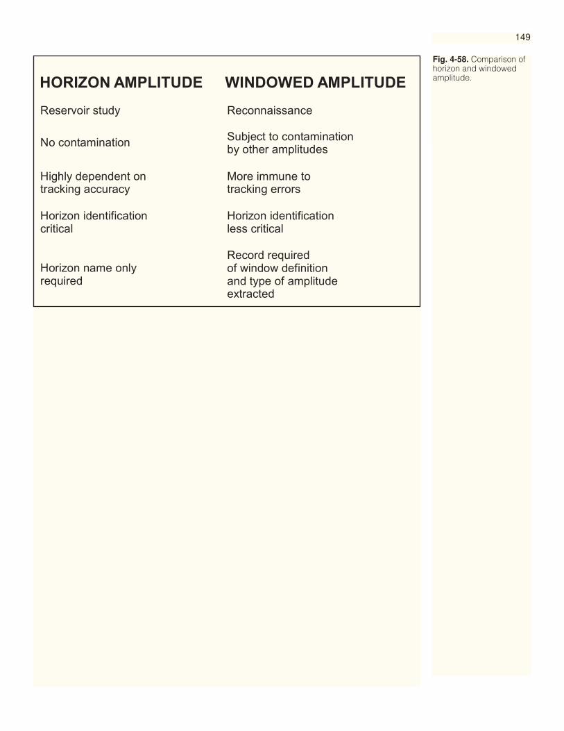
149

Fig. 4-58. Comparison ofhorizon and windowedamplitude.

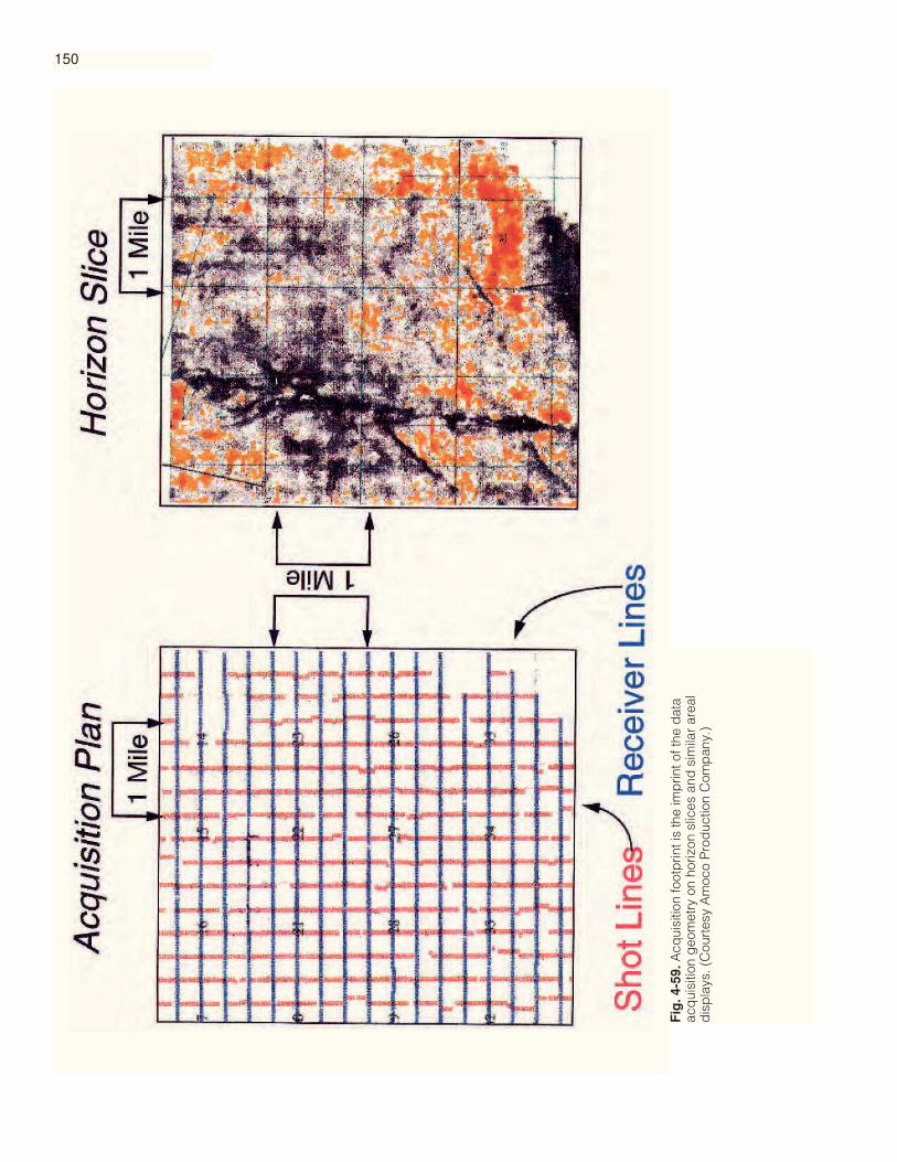
150

Fig

. 4-5

9.A

cqui

sitio

n fo

otp

rint i

s th

e im

prin

t of t

he d

ata

acq

uisi

tion

geo

met

ry o

n ho

rizon

slic

es a

nd s

imila

r ar

eal

dis

pla

ys. (

Cou

rtes

y A

moc

o P

rod

uctio

n C

omp

any.

)

151

is a very large window, but the RMS calculation helped overcome the contamination.The objectives were high-amplitude bright spots, and squaring them made them rela-tively even higher, helping them stand out against the background.

Figure 4-56 is again RMS amplitude but over a 50 ms window surrounding the rel-evant reflection. Here, Lamers and Carmichael (1999) have mapped the Top Balderreflection over multiple 3-D surveys in a reconnaissance of the Faroe Basin on theU.K. Atlantic margin. The patterns in amplitude have helped unravel the depositionalhistory of the Faroe Basin and have provided a regional understanding of this Pale-ocene deep-water play.

Figure 4-57 shows average absolute amplitude from the San Jorge Basin of south-ern Argentina. Here there are many thin reservoir sands, but they occur over a verythick interval. The 250 ms window used here was referenced to an interpreted hori-zon just below the producing interval. The individual sands are very difficult to studyseismically, but Figure 4-57 makes it clear that the productive wells are in areas of rel-atively low amplitude over the whole interval.

Average absolute amplitude, RMS amplitude, and other windowed amplitudeattributes are, as illustrated above, most beneficially used for some kind of reconnais-sance investigation. When reservoir reflections have been identified and the intent isto study the reservoir, then horizon amplitude is normally preferable. The author rec-ommends tracking the top reflection and the base reflection and extracting the hori-zon amplitude on both of them. This idea is developed further in Chapter 7.

Figure 4-58 summarizes the advantages and disadvantages of horizon and win-dowed amplitude. Horizon amplitude is generally more precise and detailed, but itdepends critically on the accuracy of the tracking, the horizon identification, and thedata phase. In using windowed amplitude it is important that the interpreter keep anaccurate record of the window definition and the type of amplitude extracted. Theplethora of attributes and windows available today increases the need for full docu-mentation.

Seismic data acquisition and processing should be conducted in a very regularmanner. We want to interpret visible irregularities in the data in terms of geology; wedo not want spatial irregularities to indicate the variations in the acquisition or pro-cessing operation. Ideally we would like every bin to be filled with the same numberof recorded traces with the same offset distribution and with the same azimuth distri-bution. This is essentially impossible to achieve within a reasonable budget. If any orall of these vary in some spatially systematic way, then the data acquisition geometryis often visible in the data as a footprint.

Figure 4-59 shows a severe footprint on a horizon slice extracted from land data.Shot lines and receiver lines are typically laid out perpendicular to each other onland, causing this kind of grid-like pattern. Marine data typically have a rather linearfootprint aligned in the direction of boat movement. Footprint is difficult to predictand generally very expensive to totally eliminate. The horizon slice is particularlysensitive to footprint. Often an interpreter observes a footprint in his data when hesees the first horizon slice, and this is the very time he wishes he didn’t have the prob-lem.

Workstation manipulations can help with footprint problems but rarely eliminatethem. If there is a shallower horizon that should reasonably be rather constant inamplitude, then dividing the objective horizon amplitude by this shallow horizonamplitude will normally lessen the footprint.

AcquisitionFootprint

Broussard, M. L., ed., 1975, Deltas: Houston Geological Society, 555 p.Brown, A. R., C. G. Dahm, and R. J. Graebner, 1981, A stratigraphic case history using

three-dimensional seismic data in the Gulf of Thailand: Geophysical Prospecting, v.29, p. 327-349.

Enachescu, M. E., 1993, Amplitude interpretation of 3-D reflection data: The LeadingEdge, v. 12, p. 678–685.

Gerster, R. L., 1995, The role played by 3-D and 2-D seismic data in the explorationand development of the largest oil field in Argentina: SEG Annual Meetingexpanded abstract.

Klein, G. deV., 1985, Sandstone depositional models for exploration for fossil fuels,third edition: Boston, Massachusetts, International Human Resources DevelopmentCorporation, 209 p.

Lamers, E., and S. M. M. Carmichael, 1999, The Paleocene deepwater sandstone playWest of Shetland, in A. J. Fleet and S. A. R. Boldy, eds., Petroleum geology of north-west Europe: Proceedings of the 5th Conference, The Geological Society, London, p.645-659.

Sanders, J. I., and G. Steel, 1982, Improved structural resolution from 3D surveys inAustralia: Australian Petroleum Exploration Association (APEA) Journal, v. 22, p.17-41.

152

References

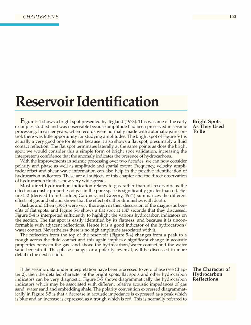
153

Reservoir IdentificationFigure 5-1 shows a bright spot presented by Tegland (1973). This was one of the early

examples studied and was observable because amplitude had been preserved in seismicprocessing. In earlier years, when records were normally made with automatic gain con-trol, there was little opportunity for studying amplitudes. The bright spot of Figure 5-1 isactually a very good one for its era because it also shows a flat spot, presumably a fluidcontact reflection. The flat spot terminates laterally at the same points as does the brightspot; we would consider this a simple form of bright spot validation, increasing theinterpreter’s confidence that the anomaly indicates the presence of hydrocarbons.

With the improvements in seismic processing over two decades, we can now considerpolarity and phase as well as amplitude and spatial extent. Frequency, velocity, ampli-tude/offset and shear wave information can also help in the positive identification ofhydrocarbon indicators. These are all subjects of this chapter and the direct observationof hydrocarbon fluids is now very widespread.

Most direct hydrocarbon indication relates to gas rather than oil reservoirs as theeffect on acoustic properties of gas in the pore space is significantly greater than oil. Fig-ure 5-2 (derived from Gardner, Gardner, and Gregory, 1974) summarizes the differenteffects of gas and oil and shows that the effect of either diminishes with depth.

Backus and Chen (1975) were very thorough in their discussion of the diagnostic ben-efits of flat spots, and Figure 5-3 shows a flat spot at 1.47 seconds that they discussed.Figure 5-4 is interpreted sufficiently to highlight the various hydrocarbon indicators onthe section. The flat spot is easily identified by its flatness, and because it is uncon-formable with adjacent reflections. Hence it is a good indicator of the hydrocarbon/water contact. Nevertheless there is no high amplitude associated with it.

The reflection from the top of the reservoir (Figure 5-4) changes from a peak to atrough across the fluid contact and this again implies a significant change in acousticproperties between the gas sand above the hydrocarbon/water contact and the watersand beneath it. This phase change, or a polarity reversal, will be discussed in moredetail in the next section.

If the seismic data under interpretation have been processed to zero phase (see Chap-ter 2), then the detailed character of the bright spots, flat spots and other hydrocarbonindicators can be very diagnostic. Figure 5-5 shows diagrammatically the hydrocarbonindicators which may be associated with different relative acoustic impedances of gassand, water sand and embedding shale. The polarity convention expressed diagrammat-ically in Figure 5-5 is that a decrease in acoustic impedance is expressed as a peak whichis blue and an increase is expressed as a trough which is red. This is normally referred to

Bright SpotsAs They Used To Be

The Character ofHydrocarbonReflections

CHAPTER FIVE

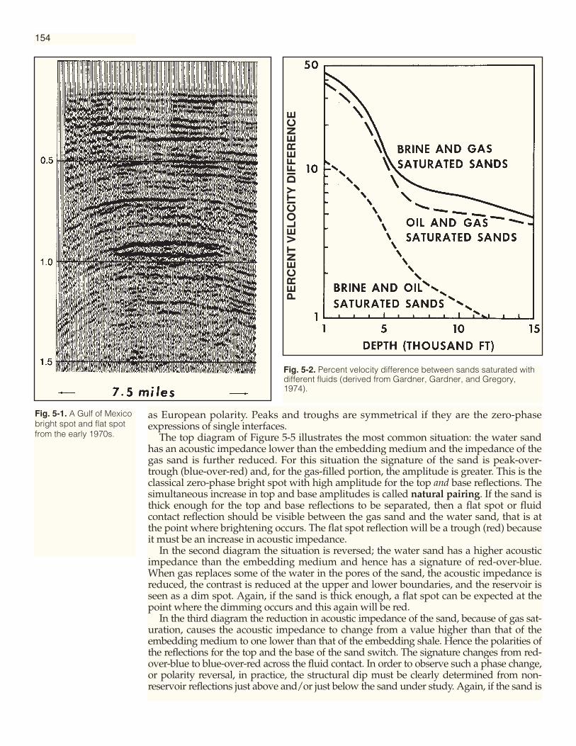
154

as European polarity. Peaks and troughs are symmetrical if they are the zero-phaseexpressions of single interfaces.

The top diagram of Figure 5-5 illustrates the most common situation: the water sandhas an acoustic impedance lower than the embedding medium and the impedance of thegas sand is further reduced. For this situation the signature of the sand is peak-over-trough (blue-over-red) and, for the gas-filled portion, the amplitude is greater. This is theclassical zero-phase bright spot with high amplitude for the top and base reflections. Thesimultaneous increase in top and base amplitudes is called natural pairing. If the sand isthick enough for the top and base reflections to be separated, then a flat spot or fluidcontact reflection should be visible between the gas sand and the water sand, that is atthe point where brightening occurs. The flat spot reflection will be a trough (red) becauseit must be an increase in acoustic impedance.

In the second diagram the situation is reversed; the water sand has a higher acousticimpedance than the embedding medium and hence has a signature of red-over-blue.When gas replaces some of the water in the pores of the sand, the acoustic impedance isreduced, the contrast is reduced at the upper and lower boundaries, and the reservoir isseen as a dim spot. Again, if the sand is thick enough, a flat spot can be expected at thepoint where the dimming occurs and this again will be red.

In the third diagram the reduction in acoustic impedance of the sand, because of gas sat-uration, causes the acoustic impedance to change from a value higher than that of theembedding medium to one lower than that of the embedding shale. Hence the polarities ofthe reflections for the top and the base of the sand switch. The signature changes from red-over-blue to blue-over-red across the fluid contact. In order to observe such a phase change,or polarity reversal, in practice, the structural dip must be clearly determined from non-reservoir reflections just above and/or just below the sand under study. Again, if the sand is

Fig. 5-1. A Gulf of Mexicobright spot and flat spotfrom the early 1970s.

Fig. 5-2. Percent velocity difference between sands saturated withdifferent fluids (derived from Gardner, Gardner, and Gregory,1974).

PE

RC

EN

T V

EL

OC

ITY

DIF

FE

RE

NC

E

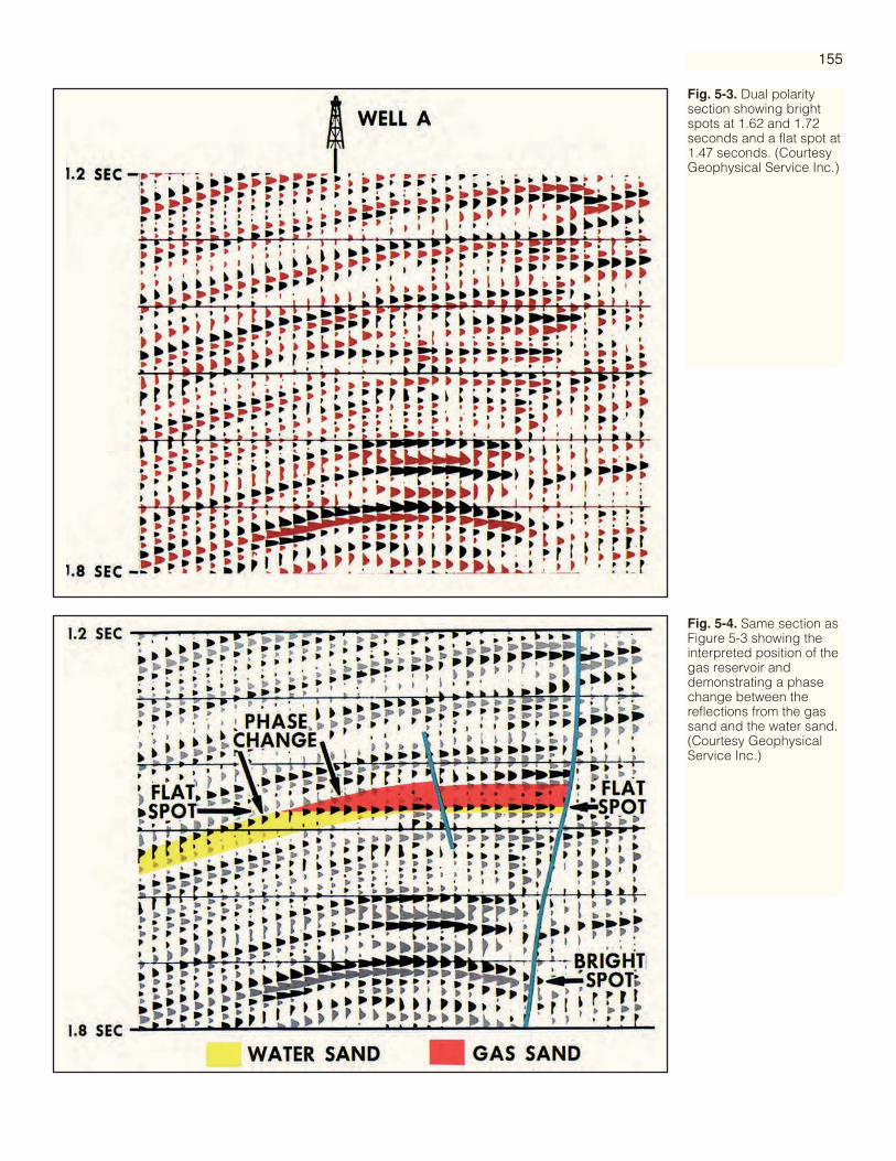
155

Fig. 5-3. Dual polaritysection showing brightspots at 1.62 and 1.72seconds and a flat spot at1.47 seconds. (CourtesyGeophysical Service Inc.)

Fig. 5-4. Same section asFigure 5-3 showing theinterpreted position of thegas reservoir anddemonstrating a phasechange between thereflections from the gassand and the water sand.(Courtesy GeophysicalService Inc.)

156

Fig. 5-5. Schematicdiagram of the zero-phaseresponse of hydrocarbonreservoirs for differentacoustic contrastsbetween the reservoir andthe embedding medium.Note these diagrams aredrawn for Europeanpolarity. Some of theexamples which follow arethus and some areAmerican polarity. Fordefinition of the two zero-phase polarities, seeFigure 2-17.

Fig. 5-6. The magnitudeof acoustic impedancechanges between water-filled and hydrocarbon-filled sands and theresulting observableindications.

157

thick enough, a fluid contact reflection should be visible and it will be red. Note that in thiscase the flat spot reflection has the highest amplitude locally.

Figure 5-6 shows the magnitude of acoustic impedance changes between water sandand hydrocarbon sand and hence the effect on seismic amplitude reflected from the inter-face between either of them and a uniform embedding medium. The diagram is drawnwith clastics in mind, but it also has generality. Tertiary sands and shales normally haverather similar acoustic properties and thus on the relative scale of Figure 5-6 lie betweenthe narrow lines, that is, not far from the heavy line of acoustic impedance equality in thecenter. For a bright spot (without phase change) the water sand is located just right of thecenter line and the gas sand is much farther to the right. For a phase change, or polarityreversal, the movement from water sand to gas sand must be from left to right across thecenter line. In the last situation illustrated in Figure 5-6, the bright spot is exactly the samein amplitude and phase as the one illustrated at the top of the figure; the difference is thatthe last one labeled phase change/bright spot combination, came from a water sand with high-er acoustic impedance than the embedding shale and was thus located on the left of thecenter line. Dim spots must start from a water sand significantly to the left on the relativescale of Figure 5-6, so that a visible movement still leaves them left of center. This is unusu-al in Tertiary clastics and thus is the reason we do not see many dim spots in that environ-ment. In older rocks, however, much greater differences in acoustic impedance betweensands and shales are normal, so that dim spots are more commonly observable.

Figure 5-7 shows a Gulf of Mexico bright spot known to be a gas reservoir. The reservoirreflections have very high amplitude and hence the interference from other nearby reflec-tions, multiples or noise is small. The bright reflections show the zero-phase response oftwo reservoir sands, each blue-over-red and located one on top of the other. The upper

Fig. 5-7. Bright and flatreflections from a Gulf ofMexico gas reservoirknown to be subdividedinto upper and lower sandunits. Data are zerophase European polarity.(Courtesy Chevron U.S.A.Inc.)

Examples of BrightSpots, Flat Spots,Dim Spots andPhase Changes

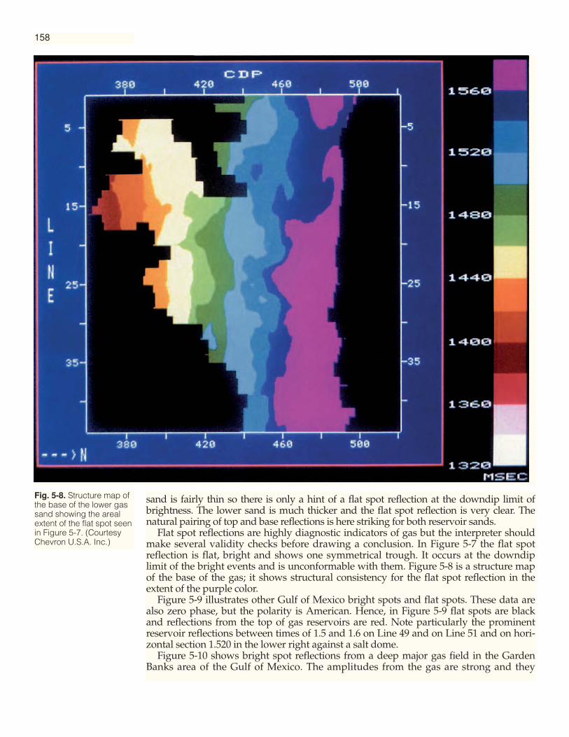
158

sand is fairly thin so there is only a hint of a flat spot reflection at the downdip limit ofbrightness. The lower sand is much thicker and the flat spot reflection is very clear. Thenatural pairing of top and base reflections is here striking for both reservoir sands.

Flat spot reflections are highly diagnostic indicators of gas but the interpreter shouldmake several validity checks before drawing a conclusion. In Figure 5-7 the flat spotreflection is flat, bright and shows one symmetrical trough. It occurs at the downdiplimit of the bright events and is unconformable with them. Figure 5-8 is a structure mapof the base of the gas; it shows structural consistency for the flat spot reflection in theextent of the purple color.

Figure 5-9 illustrates other Gulf of Mexico bright spots and flat spots. These data arealso zero phase, but the polarity is American. Hence, in Figure 5-9 flat spots are blackand reflections from the top of gas reservoirs are red. Note particularly the prominentreservoir reflections between times of 1.5 and 1.6 on Line 49 and on Line 51 and on hori-zontal section 1.520 in the lower right against a salt dome.

Figure 5-10 shows bright spot reflections from a deep major gas field in the GardenBanks area of the Gulf of Mexico. The amplitudes from the gas are strong and they

Fig. 5-8. Structure map ofthe base of the lower gassand showing the arealextent of the flat spot seenin Figure 5-7. (CourtesyChevron U.S.A. Inc.)

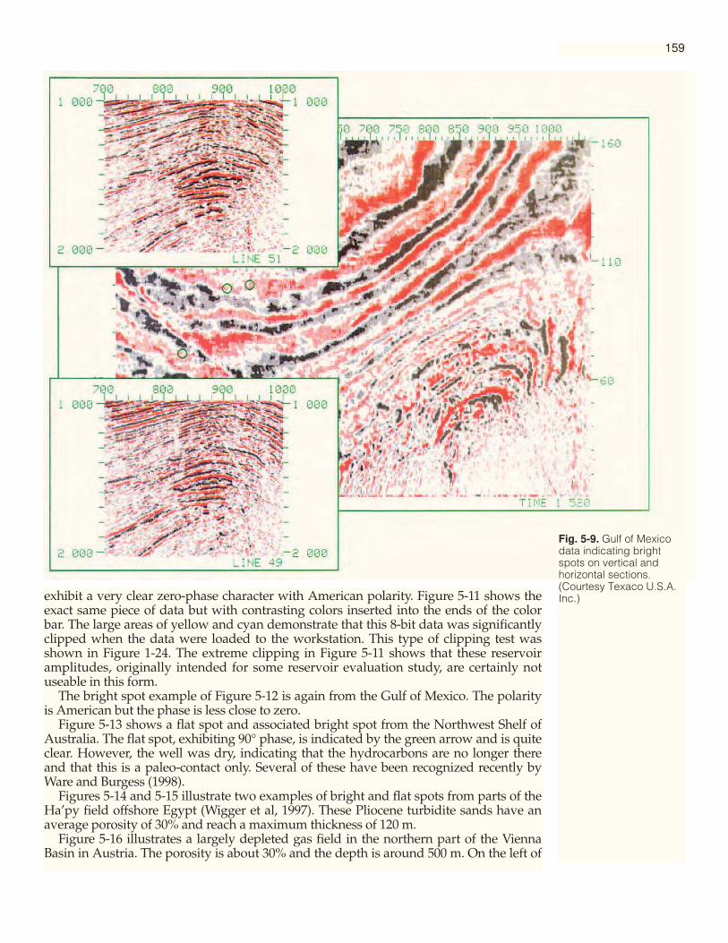
159

exhibit a very clear zero-phase character with American polarity. Figure 5-11 shows theexact same piece of data but with contrasting colors inserted into the ends of the colorbar. The large areas of yellow and cyan demonstrate that this 8-bit data was significantlyclipped when the data were loaded to the workstation. This type of clipping test wasshown in Figure 1-24. The extreme clipping in Figure 5-11 shows that these reservoiramplitudes, originally intended for some reservoir evaluation study, are certainly notuseable in this form.

The bright spot example of Figure 5-12 is again from the Gulf of Mexico. The polarityis American but the phase is less close to zero.

Figure 5-13 shows a flat spot and associated bright spot from the Northwest Shelf ofAustralia. The flat spot, exhibiting 90° phase, is indicated by the green arrow and is quiteclear. However, the well was dry, indicating that the hydrocarbons are no longer thereand that this is a paleo-contact only. Several of these have been recognized recently byWare and Burgess (1998).

Figures 5-14 and 5-15 illustrate two examples of bright and flat spots from parts of theHa’py field offshore Egypt (Wigger et al, 1997). These Pliocene turbidite sands have anaverage porosity of 30% and reach a maximum thickness of 120 m.

Figure 5-16 illustrates a largely depleted gas field in the northern part of the ViennaBasin in Austria. The porosity is about 30% and the depth is around 500 m. On the left of

Fig. 5-9. Gulf of Mexicodata indicating brightspots on vertical andhorizontal sections.(Courtesy Texaco U.S.A.Inc.)

Fig. 5-10. Bright spotsfrom four stacked Gulf ofMexico gas reservoirs.The productive sands areof Pliocene age and lie atdepths between 5000 mand 6000 m. Data arezero phase Americanpolarity. (Courtesy AmocoProduction Company.)

Fig. 5-11. Same brightspots as Figure 5-10, butcontrasting colors havebeen inserted into theextremities of the colorbar to demonstratesevere clipping of thereservoir reflections.(Courtesy AmocoProduction Company.)

160

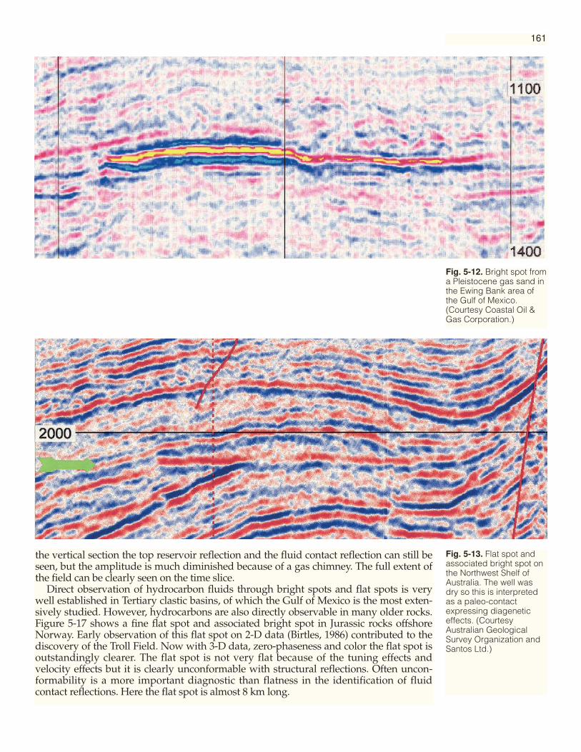
Fig. 5-12. Bright spot froma Pleistocene gas sand inthe Ewing Bank area ofthe Gulf of Mexico.(Courtesy Coastal Oil &Gas Corporation.)

161

Fig. 5-13. Flat spot andassociated bright spot onthe Northwest Shelf ofAustralia. The well wasdry so this is interpretedas a paleo-contactexpressing diageneticeffects. (CourtesyAustralian GeologicalSurvey Organization andSantos Ltd.)

the vertical section the top reservoir reflection and the fluid contact reflection can still beseen, but the amplitude is much diminished because of a gas chimney. The full extent ofthe field can be clearly seen on the time slice.

Direct observation of hydrocarbon fluids through bright spots and flat spots is verywell established in Tertiary clastic basins, of which the Gulf of Mexico is the most exten-sively studied. However, hydrocarbons are also directly observable in many older rocks.Figure 5-17 shows a fine flat spot and associated bright spot in Jurassic rocks offshoreNorway. Early observation of this flat spot on 2-D data (Birtles, 1986) contributed to thediscovery of the Troll Field. Now with 3-D data, zero-phaseness and color the flat spot isoutstandingly clearer. The flat spot is not very flat because of the tuning effects andvelocity effects but it is clearly unconformable with structural reflections. Often uncon-formability is a more important diagnostic than flatness in the identification of fluidcontact reflections. Here the flat spot is almost 8 km long.

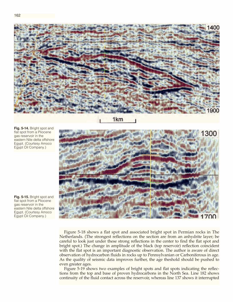
Fig. 5-14. Bright spot andflat spot from a Pliocenegas reservoir in theeastern Nile delta offshoreEgypt. (Courtesy AmocoEgypt Oil Company.)

Fig. 5-15. Bright spot andflat spot from a Pliocenegas reservoir in theeastern Nile delta offshoreEgypt. (Courtesy AmocoEgypt Oil Company.)

162

Figure 5-18 shows a flat spot and associated bright spot in Permian rocks in TheNetherlands. (The strongest reflections on the section are from an anhydrite layer; becareful to look just under these strong reflections in the center to find the flat spot andbright spot.) The change in amplitude of the black (top reservoir) reflection coincidentwith the flat spot is an important diagnostic observation. The author is aware of directobservation of hydrocarbon fluids in rocks up to Pennsylvanian or Carboniferous in age.As the quality of seismic data improves further, the age theshold should be pushed toeven greater ages.

Figure 5-19 shows two examples of bright spots and flat spots indicating the reflec-tions from the top and base of proven hydrocarbons in the North Sea. Line 182 showscontinuity of the fluid contact across the reservoir, whereas line 137 shows it interrupted

Fig. 5-16 (Upper). Verticalsection showing brightspot and flat spot from agas reservoir in upperMiocene sediments of theVienna Basin, Austria.Amplitude is lost on theleft because of a gaschimney effect. (CourtesyOMV Aktiengesellschaft.)(Lower). Time slice atlevel of flat spot showingextent of high amplitudeand extent of gaschimney. The green lineshows the alignment ofthe vertical section above.(Courtesy OMVAktiengesellschaft.)

163

in the center where the reservoir is full to base. Figure 5-20 shows horizon slices from thetop reservoir reflection and from the fluid contact/base hydrocarbon sand reflection.Similar patterns in amplitude confirm that these horizon slices indeed follow the top andbottom of the same interval.

Figure 5-21 is a practical example of a dim spot. The discovery well penetrates a gascolumn of about 400 ft (130 m) but the acoustic contrast of the gas sand with its embed-ding medium is small. Outside the reservoir the contrast between the sand and theembedding medium is much greater, as the amplitudes indicate. Here the reservoir iscemented, so the increase in acoustic impedance is caused partly by lack of gas and part-ly by the cementation. Figures 5-22 and 5-23 illustrate dim spots from the NorthwestShelf of Australia. In both cases the reservoir sands truncate at an unconformity overlain

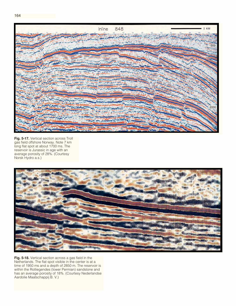
164

Fig. 5-18. Vertical section across a gas field in theNetherlands. The flat spot visible in the center is at atime of 1950 ms and a depth of 2850 m. The reservoir iswithin the Rotliegendes (lower Permian) sandstone andhas an average porosity of 18%. (Courtesy NederlandseAardolie Maatschappij B. V.)

Fig. 5-17. Vertical section across Trollgas field offshore Norway. Note 7 kmlong flat spot at about 1700 ms. Thereservoir is Jurassic in age with anaverage porosity of 28%. (CourtesyNorsk Hydro a.s.)

165

Fig. 5-19. Line 182(upper) and line 137(lower) over the Heimdalfield in the NorwegianNorth Sea. The reflectionfrom the top of the gascondensate reservoir isblue; the fluid contactreflection is red. (CourtesyElf Aquitaine Norge a/s.)

166

Fig. 5-20. Horizon slicethrough top reservoirreflection (upper) andthrough fluid contactreflection (lower) for theHeimdal field in theNorwegian North Sea.Red bar is 3 km.(Courtesy Elf AquitaineNorge a/s.)

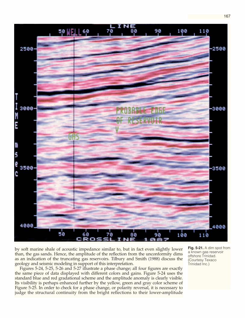
167

Fig. 5-21. A dim spot froma known gas reservoiroffshore Trinidad.(Courtesy TexacoTrinidad Inc.)

by soft marine shale of acoustic impedance similar to, but in fact even slightly lowerthan, the gas sands. Hence, the amplitude of the reflection from the unconformity dimsas an indication of the truncating gas reservoirs. Tilbury and Smith (1988) discuss thegeology and seismic modeling in support of this interpretation.

Figures 5-24, 5-25, 5-26 and 5-27 illustrate a phase change; all four figures are exactlythe same piece of data displayed with different colors and gains. Figure 5-24 uses thestandard blue and red gradational scheme and the amplitude anomaly is clearly visible.Its visibility is perhaps enhanced further by the yellow, green and gray color scheme ofFigure 5-25. In order to check for a phase change, or polarity reversal, it is necessary tojudge the structural continuity from the bright reflections to their lower-amplitude

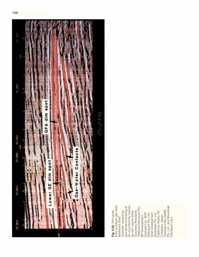
168

Fig

. 5-2

2.D

im s

pot

sfr

om G

ood

wyn

gas

fiel

d,

Nor

thw

est S

helf,

Aus

tral

ia, c

ause

d b

yg

as s

and

s tr

unca

ting

at

an u

ncon

form

ity o

verla

inb

y so

ft m

arin

e sh

ale.

(Cou

rtes

y W

ood

sid

eO

ffsho

re P

etro

leum

Pty

.,B

P D

evel

opm

ent

Aus

tral

ia L

td.,

BH

PP

etro

leum

Pty

. Ltd

.,S

hell

Dev

elop

men

t[A

ustr

alia

] P

ty. L

td.,

Cal

iforn

ia A

siat

ic O

ilC

omp

any,

Jap

anA

ustr

alia

LN

G [

MIM

I]P

ty. L

td.,

and

Woo

dsi

de

Pet

role

um L

td.)

169

Fig

. 5-2

3.D

im s

pot

from

Goo

dw

yng

as fi

eld

, Nor

thw

est S

helf,

Aus

tral

ia, t

arg

eted

as

dril

ling

loca

tion.

(C

ourt

esy

Woo

dsi

de

Offs

hore

Pet

role

um P

ty.,

BP

Dev

elop

men

t Aus

tral

ia L

td.,

BH

PP

etro

leum

Pty

. Ltd

., S

hell

Dev

elop

men

t [A

ustr

alia

] P

ty. L

td.,

Cal

iforn

ia A

siat

ic O

il C

omp

any,

Jap

an A

ustr

alia

LN

G [

MIM

I] P

ty.

Ltd

., an

d W

ood

sid

e P

etro

leum

Ltd

.)

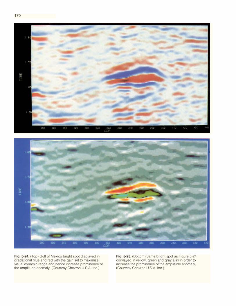
170

Fig. 5-24. (Top) Gulf of Mexico bright spot displayed ingradational blue and red with the gain set to maximizevisual dynamic range and hence increase prominence ofthe amplitude anomaly. (Courtesy Chevron U.S.A. Inc.)

Fig. 5-25. (Bottom) Same bright spot as Figure 5-24displayed in yellow, green and gray also in order toincrease the prominence of the amplitude anomaly.(Courtesy Chevron U.S.A. Inc.)

171

Fig. 5-26. (Top) Same bright spot and color scheme asFigure 5-24 but with the gain increased to study thecontinuity of reflections off the flank of the bright spot. Bluecorrelates with red and vice versa downdip indicating aphase change or polarity reversal at the edge of the brightspot. (Courtesy Chevron U.S.A. Inc.)

Fig. 5-27. (Bottom) Same bright spot as Figure 5-24, samecolor scheme as Figure 5-25 and same gain as Figure 5-26.The correlation of reflections downdip from the bright spotagain indicates a phase change at the edge of thereservoir. (Courtesy Chevron U.S.A. Inc.)

Fig. 5-28. Phase change(polarity reversal) causedby gas in unconsolidatedsandstone of the Gulf ofMexico. Data are zerophase Europeanpolarity.(Courtesy ConocoInc.)

172

equivalents downdip. There is a very great difference in amplitude between these, caus-ing a great difference in color intensity. Figures 5-26 and 5-27 use the same colors respec-tively as Figures 5-24 and 5-25 but with a higher gain applied to the data. This makes iteasier to judge the downdip continuity on the left of the bright spot and hence to observethat red correlates with blue (Figure 5-26) and green correlates with yellow (Figure 5-27).In this way a polarity reversal is established.

Figures 5-28 and 5-29 show striking phase changes (polarity reversals) respectively inthe Gulf of Mexico and on the Northwest Shelf of Australia. The two data sets are oppo-site polarity from each other. Figure 5-28 shows the gas, which is low impedance, asblue-over-red; this indicates European polarity. Figure 5-29 shows the gas as red-over-blue, which is American polarity. Figure 5-28 shows the gas contained by a fault on thewest and the phase change on the east. Figure 5-29 shows the gas contained by a fault onthe east and the phase change on the west. Some interpreters may feel inclined to identi-fy both these phase changes as faults antithetic to the main faults. However, with experi-ence the phase change explanation emerges as preferable. Structural/stratigraphic con-flicts like this one are common and interpreters need to overcome their bias towards thestructural solution.

Figure 5-30 shows the very unusual observation of a polarity reversal on the seafloor. With American polarity data, the blue reflection (with flanking red side lobes)

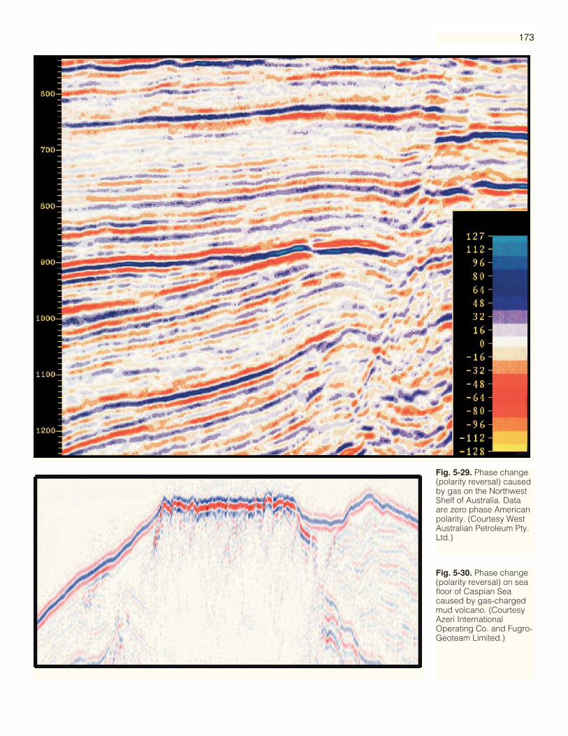
Fig. 5-29. Phase change(polarity reversal) causedby gas on the NorthwestShelf of Australia. Dataare zero phase Americanpolarity. (Courtesy WestAustralian Petroleum Pty.Ltd.)

173

Fig. 5-30. Phase change(polarity reversal) on seafloor of Caspian Seacaused by gas-chargedmud volcano. (CourtesyAzeri InternationalOperating Co. and Fugro-Geoteam Limited.)

174

Fig. 5-31. Horizon sliceshowing Gulf of Mexicochannel discussed inChapter 4. Thesuperimposed structuralcontours indicate that thebright part of the channelis shallower than the dimpart. (Courtesy ChevronU.S.A. Inc.)

indicates a hard water bottom or an impedance increase. The water bottom over themud volcano is red, which indicates an impedance decrease. The only reasonableexplanation is that this impedance decrease is caused by a strong velocity decreaseand a small density increase.

Figure 5-31 shows a horizon slice indicating a channel. To the northeast the channel isbright, to the southwest it is not. The structural contours for this horizon have beensuperimposed and they demonstrate that the bright part of the channel is structurallyabove the dim part. This combination of structural and stratigraphic information helpsvalidate gas content. Figure 5-32 is another way of graphically illustrating the same rela-tionship; the representation of the channel in amplitude is superimposed on the struc-tural configuration of the horizon surface.

The fit of amplitude to structure is a valuable hydrocarbon diagnostic. This isnormally studied by displaying amplitude spatially and overlaying the structural

175

Fig. 5-32. Combination ofthe same horizon amplitudeand structural informationas Figure 5-31 usingdifferent colors and a three-dimensional perspectivesurface. (Courtesy ChevronU.S.A. Inc.)

contours. Both Figures 5-33 and 5-34 show some fit of amplitude to structure in thisway. However, it should be remembered that this is just one of several importanthydrocarbon diagnostics; it is not essential. Luchford (2001) discusses the subject indetail and presents three examples.

Figure 5-35 demonstrates gas velocity sag on a flat spot reflection. The trough (redevent) dipping west between 1560 and 1600 ms should presumably be flat in depth butis depressed in time by the increased travel through the low velocity, wedge-shaped gassand. Flat spot dip caused in this way will always be in the opposite direction to struc-tural dip. Figure 5-36 is another example of gas velocity sag. Here the high amplitudesare still in blue and red but the lower amplitudes are expressed in gradational graytones. This provides the double benefit of highlighting the bright reflections and alsohelping establish fault definition by increasing the visibility of low amplitude event ter-minations. This section also demonstrates another phenomenon: there are bright eventswithin the reservoir which have little expression outside. This illumination of internallayering is fairly common in clastic reservoirs and is discussed further in Chapter 7.

The character of paired high-amplitude reflections, red-over-blue or blue-over-red,is an important hydrocarbon diagnostic once the polarity of the data is known. Thischapter has already presented examples of bright spots in both American and Euro-pean polarity. In Figure 5-37 two high-amplitude blue reflections were tracked andthe amplitude extracted to produce two horizon slices. Both high-amplitude patches

Polarity and PhaseProblems,Multiple Contactsand TransmissionEffects

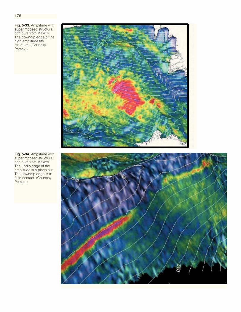
176

Fig. 5-33. Amplitude withsuperimposed structuralcontours from Mexico.The downdip edge of thehigh amplitude fitsstructure. (CourtesyPemex.)

Fig. 5-34. Amplitude withsuperimposed structuralcontours from Mexico.The updip edge of theamplitude is a pinch out.The downdip edge is afluid contact. (CourtesyPemex.)

Fig. 5-35. Bright spot froma rather thick andcomplex gas sand. Thered event dipping right-to-left is a flat spotdisplaying gas velocitysag. (Courtesy ChevronU.S.A. Inc.)

177

were drilled, but one well was successful and the other dry. These data are Americanpolarity, so red-over-blue indicates a low-impedance layer and blue-over-red indi-cates a high-impedance layer. A hydrocarbon bright spot can only be caused by lowimpedance.

The majority of the discussion of the detailed character of hydrocarbon reflectionsso far in this chapter has been of zero-phase character. Unfortunately data phase isnot always what it is supposed to be. Data processed to zero phase fairly often is closeto 90˚ phase. Figure 2-25 shows a 90˚ phase flat spot and associated bright spot. It isthe red and blue reflections together forming the flat spot that best demonstrates the90˚-phaseness of these data. Figure 2-28 shows the 90˚ phase response of a thin gasreservoir. The three events for the two interfaces (top and base reservoir) indicate the90˚-phaseness as discussed in Chapter 2.

178

Fig. 5-36. Bright spotshowing similarphenomena to Figure 5-35; the loweramplitudes are heredisplayed in gray tones.(Courtesy Chevron U.S.A.Inc.)

Figure 5-38 shows a flat spot with 90˚ phase character, yellow-over-red, at the greenarrow. This is further confused, e.g. by comparison with Figure 2-25, by the fact that herethe flat spot appears to be broken into four pieces. This is in fact caused by interference ofstrong internal reflections with the fluid contact reflection.

When we observe what appears to be two flat spots (e.g. Figures 2-25 and 5-38) thequestion arises as to whether we could be seeing two fluid contact reflections, for exam-ple gas-oil and oil-water. In fact a fluid contact is always an increase in acousticimpedance and thus two contacts in the same reservoir will always have the same char-acter; so one red contact and one blue contact is impossible.

Figure 5-39 shows two flat spots at the green arrows indicating two contacts in anIndonesian gas reservoir. They are both red. In fact the upper contact is at the base of

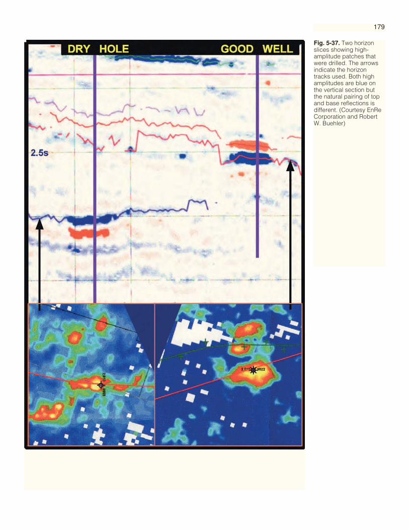
179

Fig. 5-37. Two horizonslices showing high-amplitude patches thatwere drilled. The arrowsindicate the horizontracks used. Both highamplitudes are blue onthe vertical section butthe natural pairing of topand base reflections isdifferent. (Courtesy EnReCorporation and RobertW. Buehler)

Fig. 5-38. Flat spot andbright spot visible in 90°phase data from offshoreChina. (Courtesy Bureauof GeophysicalProspecting, People’sRepublic of China.)

180

producible gas and the lower contact is at the base of trapped gas, perhaps a paleogas-water contact.

Figures 5-40 and 5-41 each show two flat spots from two separate contacts. The upperone is a gas-oil contact and the lower one an oil-water contact. Note that both fluid con-tact reflections are blue, as they should be for American polarity zero-phase data. Notethe strong structurally dipping reflection separating the upper and lower reservoirs.They have a common oil-water contact, and the gas-oil contact is only in the upper reser-voir. The somewhat high amplitude on the top reservoir reflection between the two flatspots demonstrates a bright response of oil. The difference in amplitude of the oil and thegas is clear with the higher dynamic range color scheme of Figure 5-41. Clark (1992) andGreenlee et al. (1994) have both demonstrated bright spots caused by oil.

Figure 5-42 demonstrates a hydrocarbon transmission effect. The amplitude of theupper reservoir is very strong. This means that a large fraction of the incident energyis reflected, leaving little energy to be transmitted. This effect causes a marked reduc-tion in amplitude for the lower reservoir. The coincidence of the high amplitude at theupper reservoir with lower amplitude at the lower reservoir is confirmed spatiallywith the two horizon slices of Figures 5-43 and 5-44.

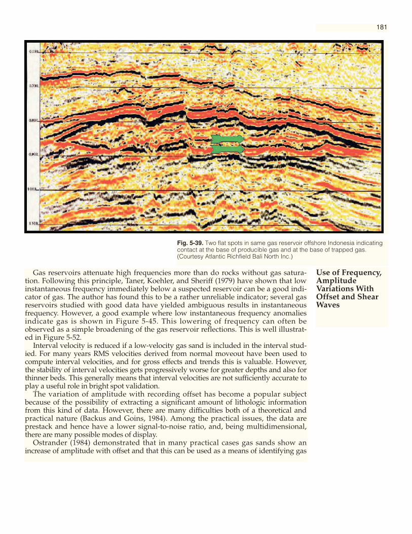
Fig. 5-39. Two flat spots in same gas reservoir offshore Indonesia indicatingcontact at the base of producible gas and at the base of trapped gas.(Courtesy Atlantic Richfield Bali North Inc.)

181

Gas reservoirs attenuate high frequencies more than do rocks without gas satura-tion. Following this principle, Taner, Koehler, and Sheriff (1979) have shown that lowinstantaneous frequency immediately below a suspected reservoir can be a good indi-cator of gas. The author has found this to be a rather unreliable indicator; several gasreservoirs studied with good data have yielded ambiguous results in instantaneousfrequency. However, a good example where low instantaneous frequency anomaliesindicate gas is shown in Figure 5-45. This lowering of frequency can often beobserved as a simple broadening of the gas reservoir reflections. This is well illustrat-ed in Figure 5-52.

Interval velocity is reduced if a low-velocity gas sand is included in the interval stud-ied. For many years RMS velocities derived from normal moveout have been used tocompute interval velocities, and for gross effects and trends this is valuable. However,the stability of interval velocities gets progressively worse for greater depths and also forthinner beds. This generally means that interval velocities are not sufficiently accurate toplay a useful role in bright spot validation.

The variation of amplitude with recording offset has become a popular subjectbecause of the possibility of extracting a significant amount of lithologic informationfrom this kind of data. However, there are many difficulties both of a theoretical andpractical nature (Backus and Goins, 1984). Among the practical issues, the data areprestack and hence have a lower signal-to-noise ratio, and, being multidimensional,there are many possible modes of display.

Ostrander (1984) demonstrated that in many practical cases gas sands show anincrease of amplitude with offset and that this can be used as a means of identifying gas

Use of Frequency,AmplitudeVariations WithOffset and ShearWaves

Fig. 5-40. Vertical section from offshore Nigeria showing flat spots from the gas-oil contact and the oil-water contact in the same reservoir. Notethe significant bright spot from the oil. The flat spot from the oil-water contact is more than 2km long. (Courtesy Mobil Producing Nigeria Ltd.)

Fig. 5-41. Same section as Figure 5-40 but with higher dynamic range color scheme which more clearly distinguishes the amplitudesfrom the gas and from the oil. (Courtesy Mobil Producing Nigeria Ltd.)

182

183

Fig. 5-42. Section fromoffshore Mexicodemonstrating transmissioneffect. Because Sahil 1 gasreservoir has very highamplitude, little energy istransmitted, and Sahil 2gas reservoir showsconsequentially reducedamplitude. (CourtesyPemex.)

Fig. 5-43. (Below) Horizon slice Sahil 1. Thewhite lines are manually drawn around thehigh-amplitude areas. (Courtesy Pemex.)

Fig. 5-44. (Below) Horizon slice Sahil 2. The outlines arerepeated from Fig. 5-43 demonstrating that high-amplitudeareas at Sahil 1 correspond to low-amplitude areas at Sahil 2.(Courtesy Pemex.)

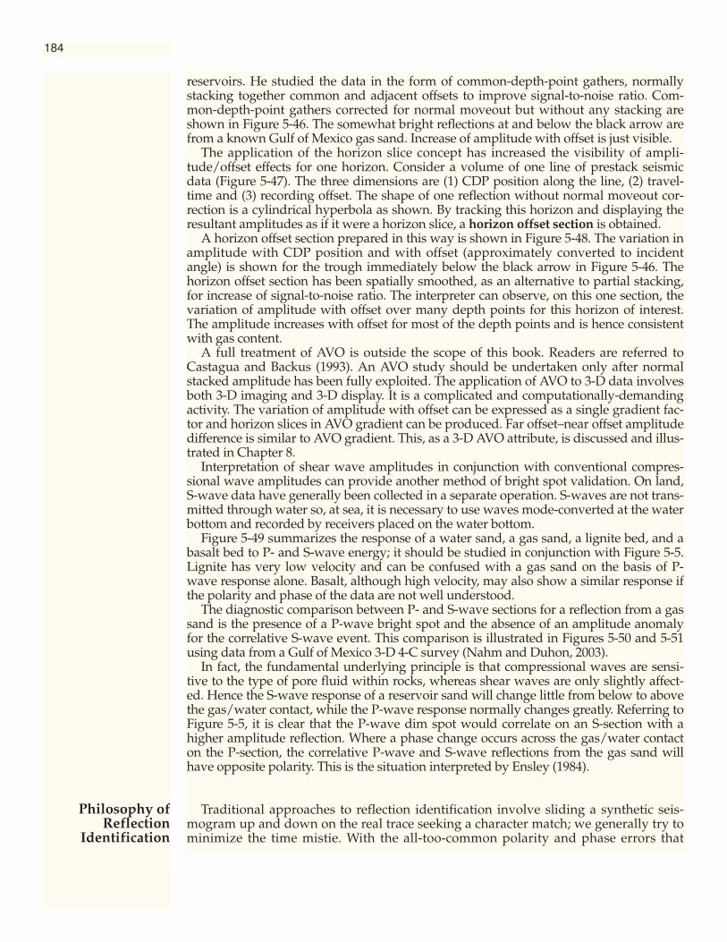
reservoirs. He studied the data in the form of common-depth-point gathers, normallystacking together common and adjacent offsets to improve signal-to-noise ratio. Com-mon-depth-point gathers corrected for normal moveout but without any stacking areshown in Figure 5-46. The somewhat bright reflections at and below the black arrow arefrom a known Gulf of Mexico gas sand. Increase of amplitude with offset is just visible.

The application of the horizon slice concept has increased the visibility of ampli-tude/offset effects for one horizon. Consider a volume of one line of prestack seismicdata (Figure 5-47). The three dimensions are (1) CDP position along the line, (2) travel-time and (3) recording offset. The shape of one reflection without normal moveout cor-rection is a cylindrical hyperbola as shown. By tracking this horizon and displaying theresultant amplitudes as if it were a horizon slice, a horizon offset section is obtained.

A horizon offset section prepared in this way is shown in Figure 5-48. The variation inamplitude with CDP position and with offset (approximately converted to incidentangle) is shown for the trough immediately below the black arrow in Figure 5-46. Thehorizon offset section has been spatially smoothed, as an alternative to partial stacking,for increase of signal-to-noise ratio. The interpreter can observe, on this one section, thevariation of amplitude with offset over many depth points for this horizon of interest.The amplitude increases with offset for most of the depth points and is hence consistentwith gas content.

A full treatment of AVO is outside the scope of this book. Readers are referred toCastagua and Backus (1993). An AVO study should be undertaken only after normalstacked amplitude has been fully exploited. The application of AVO to 3-D data involvesboth 3-D imaging and 3-D display. It is a complicated and computationally-demandingactivity. The variation of amplitude with offset can be expressed as a single gradient fac-tor and horizon slices in AVO gradient can be produced. Far offset–near offset amplitudedifference is similar to AVO gradient. This, as a 3-D AVO attribute, is discussed and illus-trated in Chapter 8.

Interpretation of shear wave amplitudes in conjunction with conventional compres-sional wave amplitudes can provide another method of bright spot validation. On land,S-wave data have generally been collected in a separate operation. S-waves are not trans-mitted through water so, at sea, it is necessary to use waves mode-converted at the waterbottom and recorded by receivers placed on the water bottom.

Figure 5-49 summarizes the response of a water sand, a gas sand, a lignite bed, and abasalt bed to P- and S-wave energy; it should be studied in conjunction with Figure 5-5.Lignite has very low velocity and can be confused with a gas sand on the basis of P-wave response alone. Basalt, although high velocity, may also show a similar response ifthe polarity and phase of the data are not well understood.

The diagnostic comparison between P- and S-wave sections for a reflection from a gassand is the presence of a P-wave bright spot and the absence of an amplitude anomalyfor the correlative S-wave event. This comparison is illustrated in Figures 5-50 and 5-51using data from a Gulf of Mexico 3-D 4-C survey (Nahm and Duhon, 2003).

In fact, the fundamental underlying principle is that compressional waves are sensi-tive to the type of pore fluid within rocks, whereas shear waves are only slightly affect-ed. Hence the S-wave response of a reservoir sand will change little from below to abovethe gas/water contact, while the P-wave response normally changes greatly. Referring toFigure 5-5, it is clear that the P-wave dim spot would correlate on an S-section with ahigher amplitude reflection. Where a phase change occurs across the gas/water contacton the P-section, the correlative P-wave and S-wave reflections from the gas sand willhave opposite polarity. This is the situation interpreted by Ensley (1984).

Traditional approaches to reflection identification involve sliding a synthetic seis-mogram up and down on the real trace seeking a character match; we generally try tominimize the time mistie. With the all-too-common polarity and phase errors that

184

Philosophy ofReflection

Identification

may exist in our data, a more general and flexible approach will be more reliable. Letus not simply assume that the data phase and polarity are what they are supposed tobe. The interpreter should attempt to assess them in, for example, the ways discussedin Chapter 2. If synthetic seismograms are used, then ones made with many differentphases of wavelet should be compared to the real data. Color is very helpful in detect-ing detailed character and recognizing phase and polarity errors.

The interpreter should be able to understand the complete character of the seismicdata in the region of the geologic interface being tied. All the local reflections need tobe understood; the more they cannot be understood, the more questions hang overthe reflection identification. Clearly we must be confident of our reflection identifica-tion before any reservoir evaluation or characterization project, based on that reflec-tion, can have any chance of success.

Let us consider an example: we find a seismic event of the right polarity (we think)at approximately the right time, so this becomes the top reservoir reflection. We knowthe approximate thickness of our reservoir so we look at the appropriate number ofmilliseconds deeper to find the reflection from the base. We find one of the rightpolarity at approximately the right time, so this becomes the base reservoir reflection.We know that we will need both top and base reflections for the study which is pend-ing. All the wells show that the reservoir is a single, fairly massive unit so we wouldnot expect any significant reflections from internal layers. However, on the seismicdata, there is a reflection between top reservoir and base reservoir whose amplitude is

Fig. 5-45. Instantaneousfrequency sectionshowing several lowfrequency indications ofgas in red. (CourtesyApache Corporation.)

185

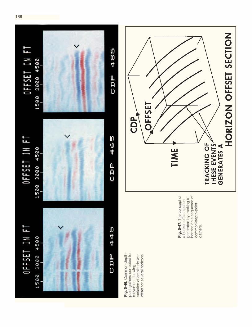
186

Fig

. 5-4

6.C

omm

on-d

epth

-p

oint

gat

hers

cor

rect

ed fo

rm

ovem

ent s

how

ing

varia

tion

of a

mp

litud

e w

ithof

fset

for

seve

ral h

oriz

ons.

Fig

. 5-4

7.Th

e co

ncep

t of

a ho

rizon

offs

et s

ectio

ng

ener

ated

by

trac

king

aho

rizon

on

a se

que

nce

ofco

mm

on-d

epth

-poi

ntg

athe

rs.

187

Fig

. 5-4

8.H

oriz

on o

ffset

sec

tion

for

a G

ulf

of M

exic

o b

right

sp

ot s

how

ing

incr

ease

of

amp

litud

e w

ith o

ffset

for

mos

t dep

th p

oint

s.

188

greater than either top or base. Furthermore this “internal” reflection is widespread.The fact that we can then provide no satisfactory explanation for this reflectionthrows into question all the previous reflection identification!

Some general recommendations for seismic reflection identification then include:

• Don't assume the data polarity and phase are what they are supposed to be.

• If you are going to use synthetic seismograms, use a suite of seismograms of vari-ous phases and of both polarities.

• Use a double-gradational color display which is balanced, because much moredetailed character will be visible and you will more readily recognize polarity andphase problems.

• Consider all the local character, that is, seek to explain all the reflections in theneighborhood of the objective.

• Don’t worry too much about time misties; they can usually be explained.

Fig. 5-49. Schematicdiagram of the P-waveand S-wave zero-phaseresponse for differentbeds encased in shale.

189

Fig. 5-50. Bright spotindicating gas fromEast Cameron area ofGulf of Mexico. This isthe normalcompressional wavesection. (Courtesy BP.)

Fig. 5-51.Correspondingconverted wavesection from four-component survey.The gas bright spot isnot present but rathera dimming inamplitude appears tooccur. (Courtesy BP.)

( 1) Is the reflection from the suspected reservoir anomalous in amplitude?( 2) Do the high-amplitude reflections have the character expected for hydrocarbons

in these data?( 3) Is the amplitude anomaly structurally consistent?( 4) Is there one reflection from the top of the reservoir and one from the base?( 5) Do the top and base reflections exhibit natural pairing, dimming at the same

point at the edge of the reservoir?( 6) Is the amplitude of the anomaly large relative to the background?( 7) Are the data zero phase and known polarity?( 8) Is a flat spot visible and is it discrete?( 9) Is the flat spot flat or dipping consistent with gas velocity sag or tuning?(10) Is the flat spot unconformable with the structure but consistent with it?(11) Does the flat spot have the correct zero-phase character?(12) Is the flat spot located at the downdip limit of the anomaly?(13) Is a phase change (polarity reversal) visible?(14) Is the phase change structurally consistent and at the same level as the flat spot?(15) Does bright spot, dim spot, or phase change show the appropriate zero-phase

character?(16) Is there a broadening of the reservoir reflections or a low-frequency shadow

below?(17) If the reservoir is thick, are there significant reflections inside?(18) Do amplitude versus offset studies yield further validation evidence?(19) Do shear wave or converted wave data provide further validation evidence?(20) Do statistical crossplotting techniques indicate a flat spot?(21) Is there an anomaly in moveout-derived interval velocity?

Every hydrocarbon indicator is potentially a reservoir, but any one indication can bespurious. Confident identification of a hydrocarbon necessarily involves the accumula-tion of evidence. The more questions on the above list to which you can answer “Yes,”the greater should be your confidence. Every negative answer needs to be satisfactorilyexplained or the identification falls into question.

Figure 5-52 contains several suspected hydrocarbon reservoirs. Try asking the abovequestions for these data. You should find affirmative answers for questions 1 through 17for many separate reservoirs. How many did you find? While scrutinizing these data, itis useful to bear in mind simple reservoir models, such as those portrayed in Figure 5-5.An effective way to interpret the reservoirs from Figure 5-52 is to draw an overlay for thereservoir reflections. On the assumption of zero-phaseness, interfaces should be drawnalong crestal amplitudes, and it is important to mark the top and bottom of each suspect-ed hydrocarbon reservoir and the top and bottom of the correlative aquifer in each case.

For comparison with Figure 5-52, Figure 5-53 presents the same data at a normal dis-play aspect ratio and in variable area/wiggle trace. This demonstrates not only the valueof color for identifying the reservoir reflections in Figure 5-52 but also the value of anexpanded vertical scale.

Figure 5-54 presents the same section as Figure 5-52, but with the results of a wellinserted. This demonstrates that there are at least seven stacked gas reservoirs at this off-shore California location.

The nature of hydrocarbon indication — that is, whether the phenomenon is brightspot, phase change, or dim spot — depends on the relative acoustic impedances ofhydrocarbon sand, water sand, and shale (Figure 5-5). Each of these acoustic impedancesincreases with depth (Figure 5-55) and they also each increase with rock age. It is difficultto be quantitative because they are also dependent on lithology, porosity, and local envi-ronment. Figure 5-55 is thus plotted for the qualitative product of depth and age. Theeffect of compaction on the shale causes its acoustic impedance to increase less rapidly

190

Questions anInterpreter ShouldAsk in an Attempt

to Validate thePresence of

Hydrocarbons

The Occurrence ofHydrocarbon

Indicators

191

Fig. 5-52. Hydrocarbonindicators offshoreCalifornia. It is intendedthat the reader interrogatethis section with the“Questions an interpretershould ask in an attemptto validate the presenceof hydrocarbons.”

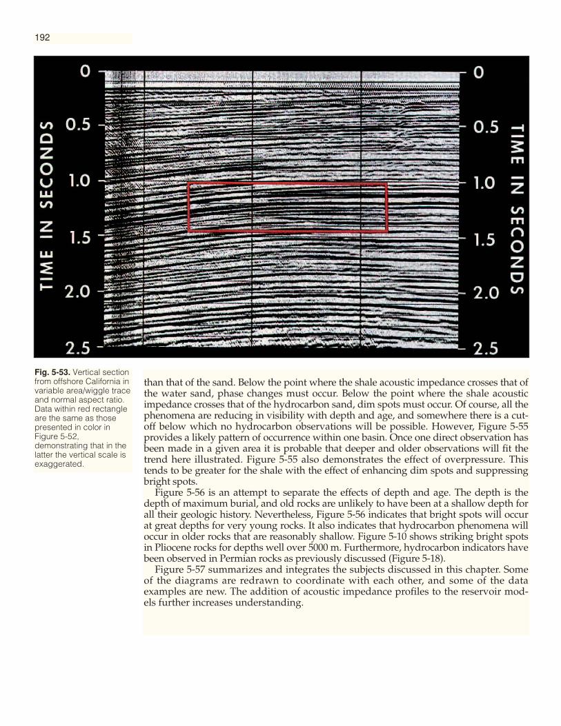
192

Fig. 5-53. Vertical sectionfrom offshore California invariable area/wiggle traceand normal aspect ratio.Data within red rectangleare the same as thosepresented in color inFigure 5-52,demonstrating that in thelatter the vertical scale isexaggerated.

than that of the sand. Below the point where the shale acoustic impedance crosses that ofthe water sand, phase changes must occur. Below the point where the shale acousticimpedance crosses that of the hydrocarbon sand, dim spots must occur. Of course, all thephenomena are reducing in visibility with depth and age, and somewhere there is a cut-off below which no hydrocarbon observations will be possible. However, Figure 5-55provides a likely pattern of occurrence within one basin. Once one direct observation hasbeen made in a given area it is probable that deeper and older observations will fit thetrend here illustrated. Figure 5-55 also demonstrates the effect of overpressure. Thistends to be greater for the shale with the effect of enhancing dim spots and suppressingbright spots.

Figure 5-56 is an attempt to separate the effects of depth and age. The depth is thedepth of maximum burial, and old rocks are unlikely to have been at a shallow depth forall their geologic history. Nevertheless, Figure 5-56 indicates that bright spots will occurat great depths for very young rocks. It also indicates that hydrocarbon phenomena willoccur in older rocks that are reasonably shallow. Figure 5-10 shows striking bright spotsin Pliocene rocks for depths well over 5000 m. Furthermore, hydrocarbon indicators havebeen observed in Permian rocks as previously discussed (Figure 5-18).

Figure 5-57 summarizes and integrates the subjects discussed in this chapter. Someof the diagrams are redrawn to coordinate with each other, and some of the dataexamples are new. The addition of acoustic impedance profiles to the reservoir mod-els further increases understanding.

193

Fig. 5-54. Same sectionas Figure 5-52 with resultsof well inserted.

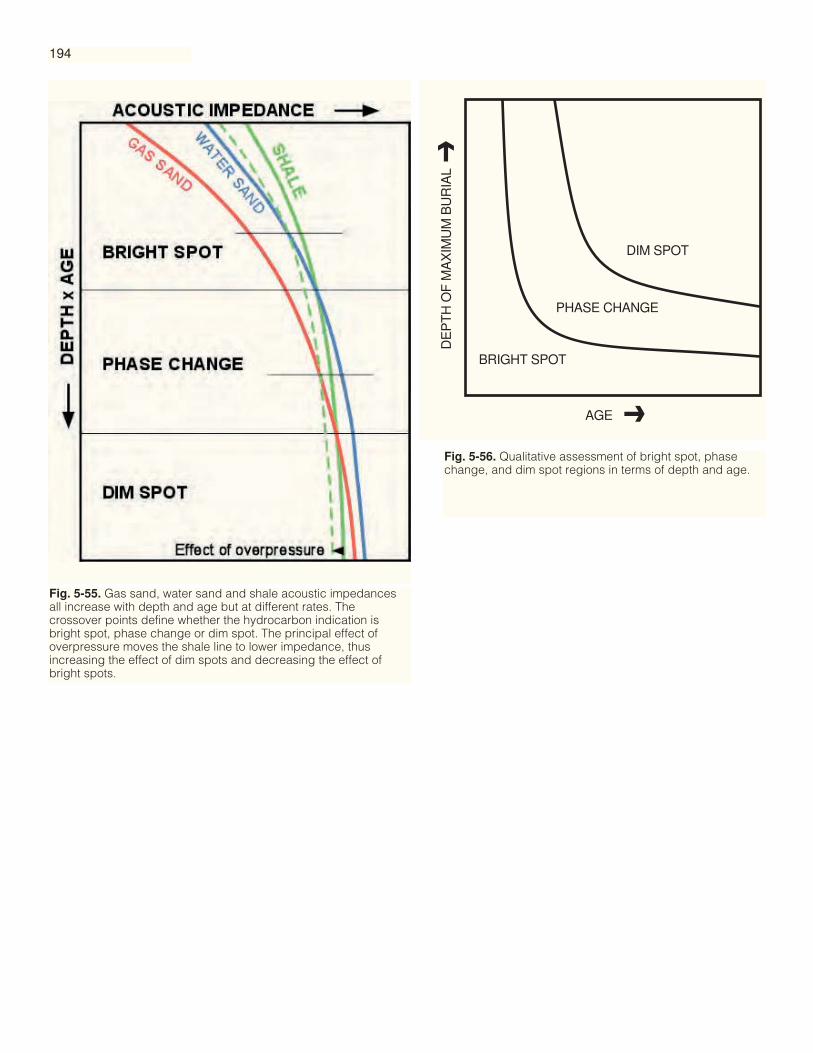
194

DIM SPOT

PHASE CHANGE

BRIGHT SPOT

AGE

DE

PT

H O

F M

AX

IMU

M B

UR

IAL

Fig. 5-55. Gas sand, water sand and shale acoustic impedancesall increase with depth and age but at different rates. Thecrossover points define whether the hydrocarbon indication isbright spot, phase change or dim spot. The principal effect ofoverpressure moves the shale line to lower impedance, thusincreasing the effect of dim spots and decreasing the effect ofbright spots.

Fig. 5-56. Qualitative assessment of bright spot, phasechange, and dim spot regions in terms of depth and age.

195

Backus, M. M., and R. L. Chen, 1975, Flat spot exploration: Geophysical Prospecting, v.23, p. 533-577.

Backus, M. M., and N. Goins, 1984, Change in reflectivity with offset, Research Work-shop report: Geophysics, v. 49, p. 838-839.

Birtles, R., 1986, The seismic flat spot and the discovery and delineation of the Troll Field,in Habitat of hydrocarbons on the Norwegian continental shelf, A.M. Spencer et al.(eds.): Graham and Trotman, p. 207-215.

Castagua, J. P., and M. M. Backus, 1993, Offset-dependent reflectivity — theory and prac-tice of AVO analysis: SEG Investigations in Geophysics, No. 8, 348 p.

Clark, V. A., 1992, The effect of oil under in situ conditions on the seismic properties ofrocks: Geophysics, v. 57, p. 894–901.

Ensley, R. A., 1984, Comparison of P- and S-wave seismic data: a new method for detect-ing gas reservoirs: Geophysics, v. 49, p. 1420-1431.

Gardner, G. H. F., L. W. Gardner, and A. R. Gregory, 1974, Formation velocity and densi-ty — the diagnostic basics for stratigraphic traps: Geophysics, v. 39, p. 770-780.

Greenlee, S.M., G. M. Gaskins, and M. G. Johnson, 1994, 3-D seismic benefits from explo-ration through development — an Exxon perspective: The Leading Edge, v. 13, p. 730-734.

Luchford, J., 2001, A view of amplitude fit to structure as a hydrocarbon-indicatingattribute: First Break, v. 19, p. 411-417.

Nahm, J. W., and M. P. Duhon, 2003, Interpretation and practical applications of 4C-3Dseismic data, East Cameron gas fields, Gulf of Mexico: The Leading Edge, v. 22, p. 300-309.

O’Connell, J. K., M. Kohli, and S. W. Amos, 1990, Bullwinkle: a unique 3-D experiment:Proceedings, SEG 60th Annual Meeting, p. 756-757.

Ostrander, W. J., 1984, Plane-wave reflection coefficients for gas sands at non-normalangles of incidence: Geophysics, v. 49, p. 1637-1648.

Taner, M. T., F. Koehler, and R. E. Sheriff, 1979, Complex seismic trace analysis: Geo-physics, v. 44, p. 1041-1063.

Tegland, E. R., 1973, Utilization of computer-derived seismic parameters in direct hydro-carbon exploration and development, in Lithology and direct detection of hydrocar-bons using geophysical methods: Dallas Geophysical and Geological Societies sympo-sium.

Tilbury, L. A., and P. M. Smith, 1988, Seismic reflection amplitude (dim spot) study overthe Goodwyn Gas Field, Northwest Shelf, Australia: Proceedings, ASEG/SEG Confer-ence (Adelaide), p. 179-183.

Ware, P.L.G., and C. Burgess, 1998, The problem of paleo-oil-water-contacts in seismicidentification of hydrocarbon accumulations: AAPG International Conference, Rio deJaneiro, and Geophysical Society of Houston newsletter (January 1999).

Wigger, S.T., J. Bailey, M. Larsen, and M. Wallace, 1997, Ha’py Field: a Pliocene brightspot example from the Nile delta, Egypt: The Leading Edge, v. 16, p. 1827-1829.

References

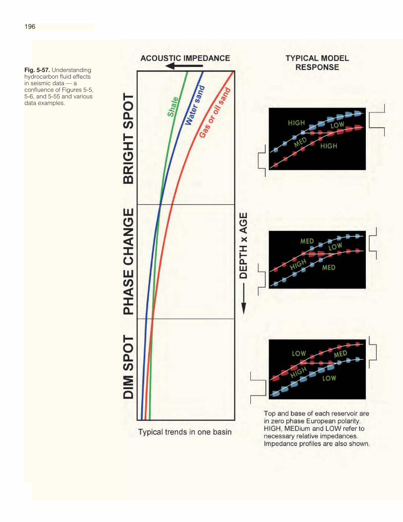
196

Fig. 5-57. Understandinghydrocarbon fluid effectsin seismic data — aconfluence of Figures 5-5,5-6, and 5-55 and variousdata examples.

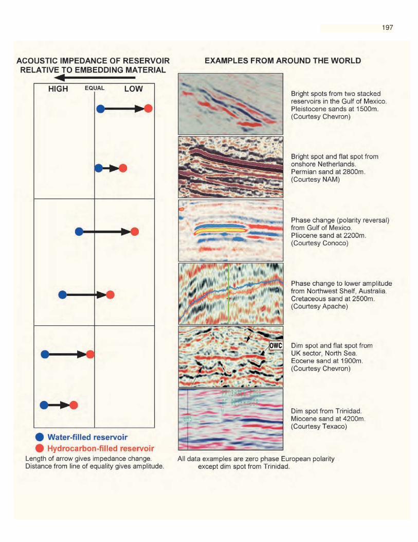
197

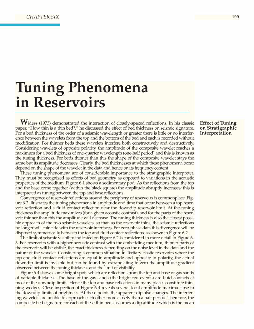
199

Tuning Phenomena in Reservoirs

Widess (1973) demonstrated the interaction of closely-spaced reflections. In his classicpaper, “How thin is a thin bed?,” he discussed the effect of bed thickness on seismic signature.For a bed thickness of the order of a seismic wavelength or greater there is little or no interfer-ence between the wavelets from the top and the bottom of the bed and each is recorded withoutmodification. For thinner beds these wavelets interfere both constructively and destructively.Considering wavelets of opposite polarity, the amplitude of the composite wavelet reaches amaximum for a bed thickness of one-quarter wavelength (one-half period) and this is known asthe tuning thickness. For beds thinner than this the shape of the composite wavelet stays thesame but its amplitude decreases. Clearly, the bed thicknesses at which these phenomena occurdepend on the shape of the wavelet in the data and hence on its frequency content.

These tuning phenomena are of considerable importance to the stratigraphic interpreter.They must be recognized as effects of bed geometry as opposed to variations in the acousticproperties of the medium. Figure 6-1 shows a sedimentary pod. As the reflections from the topand the base come together (within the black square) the amplitude abruptly increases; this isinterpreted as tuning between the top and base reflections.

Convergence of reservoir reflections around the periphery of reservoirs is commonplace. Fig-ure 6-2 illustrates the tuning phenomena in amplitude and time that occur between a top reser-voir reflection and a fluid contact reflection near the downdip reservoir limit. At the tuningthickness the amplitude maximizes (for a given acoustic contrast), and for the parts of the reser-voir thinner than this the amplitude will decrease. The tuning thickness is also the closest possi-ble approach of the two seismic wavelets, so that, as the reservoir thins, the seismic reflectionsno longer will coincide with the reservoir interfaces. For zero-phase data this divergence will bedisposed symmetrically between the top and fluid contact reflections, as shown in Figure 6-2.

The limit of seismic visibility indicated on Figure 6-2 is considered in more detail in Figure 6-3. For reservoirs with a higher acoustic contrast with the embedding medium, thinner parts ofthe reservoir will be visible, the exact thickness depending on the noise level in the data and thenature of the wavelet. Considering a common situation in Tertiary clastic reservoirs where thetop and fluid contact reflections are equal in amplitude and opposite in polarity, the actualdowndip limit is invisible but can be found by extrapolating to zero the amplitude gradientobserved between the tuning thickness and the limit of visibility.

Figure 6-4 shows some bright spots which are reflections from the top and base of gas sandsof variable thickness. The base of the gas sands (the bright red events) are fluid contacts atmost of the downdip limits. Hence the top and base reflections in many places constitute thin-ning wedges. Close inspection of Figure 6-4 reveals several local amplitude maxima close tothe downdip limits of brightness. At these points the apparent dip also changes. The interfer-ing wavelets are unable to approach each other more closely than a half period. Therefore, thecomposite bed signature for each of these thin beds assumes a dip attitude which is the mean

Effect of Tuningon StratigraphicInterpretation

CHAPTER SIX

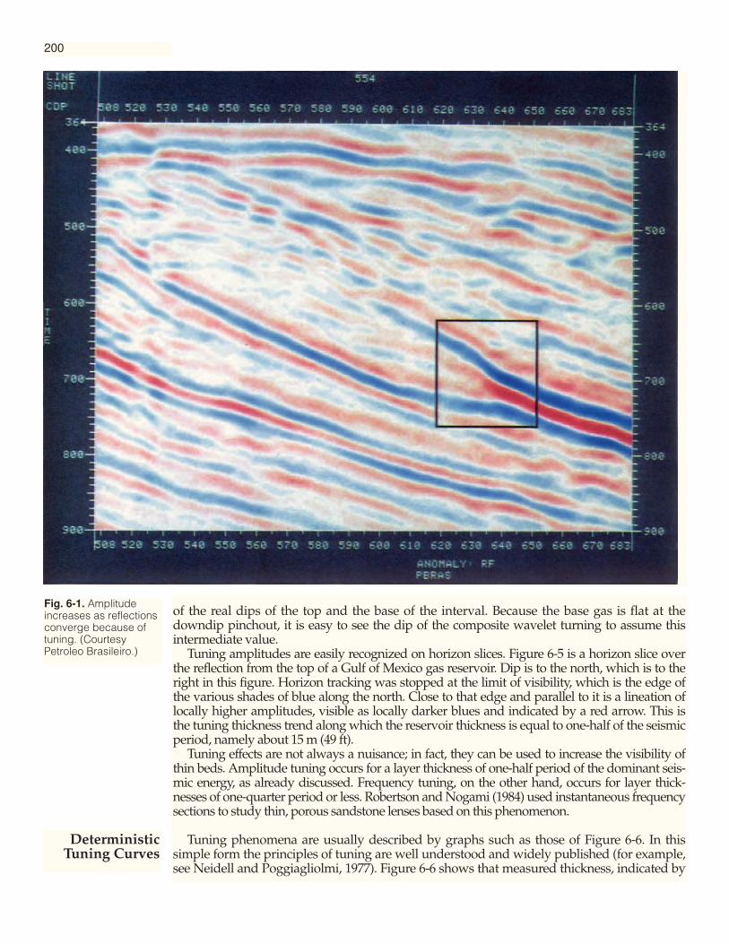
200

of the real dips of the top and the base of the interval. Because the base gas is flat at thedowndip pinchout, it is easy to see the dip of the composite wavelet turning to assume thisintermediate value.

Tuning amplitudes are easily recognized on horizon slices. Figure 6-5 is a horizon slice overthe reflection from the top of a Gulf of Mexico gas reservoir. Dip is to the north, which is to theright in this figure. Horizon tracking was stopped at the limit of visibility, which is the edge ofthe various shades of blue along the north. Close to that edge and parallel to it is a lineation oflocally higher amplitudes, visible as locally darker blues and indicated by a red arrow. This isthe tuning thickness trend along which the reservoir thickness is equal to one-half of the seismicperiod, namely about 15 m (49 ft).

Tuning effects are not always a nuisance; in fact, they can be used to increase the visibility ofthin beds. Amplitude tuning occurs for a layer thickness of one-half period of the dominant seis-mic energy, as already discussed. Frequency tuning, on the other hand, occurs for layer thick-nesses of one-quarter period or less. Robertson and Nogami (1984) used instantaneous frequencysections to study thin, porous sandstone lenses based on this phenomenon.

Tuning phenomena are usually described by graphs such as those of Figure 6-6. In thissimple form the principles of tuning are well understood and widely published (for example,see Neidell and Poggiagliolmi, 1977). Figure 6-6 shows that measured thickness, indicated by

Fig. 6-1. Amplitudeincreases as reflectionsconverge because oftuning. (CourtesyPetroleo Brasileiro.)

DeterministicTuning Curves

201

Fig. 6-2. Tuning effects inboth amplitude and timeapplicable to zero-phasewavelets for a thinningwedge such as occursbetween reservoir top andfluid contact reflectionsnear a downdip reservoirlimit.

Fig. 6-3. Limit of seismicvisibility depends onacoustic contrast ofreservoir interfaces, noiselevel and wavelet shape.(After Meckel and Nath,1977.)

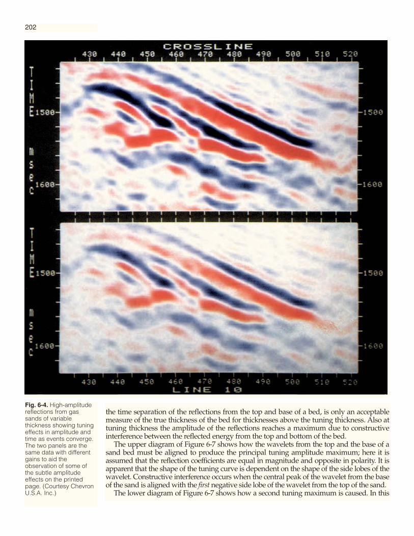
202

Fig. 6-4. High-amplitudereflections from gassands of variablethickness showing tuningeffects in amplitude andtime as events converge.The two panels are thesame data with differentgains to aid theobservation of some ofthe subtle amplitudeeffects on the printedpage. (Courtesy ChevronU.S.A. Inc.)

the time separation of the reflections from the top and base of a bed, is only an acceptablemeasure of the true thickness of the bed for thicknesses above the tuning thickness. Also attuning thickness the amplitude of the reflections reaches a maximum due to constructiveinterference between the reflected energy from the top and bottom of the bed.

The upper diagram of Figure 6-7 shows how the wavelets from the top and the base of asand bed must be aligned to produce the principal tuning amplitude maximum; here it isassumed that the reflection coefficients are equal in magnitude and opposite in polarity. It isapparent that the shape of the tuning curve is dependent on the shape of the side lobes of thewavelet. Constructive interference occurs when the central peak of the wavelet from the baseof the sand is aligned with the first negative side lobe of the wavelet from the top of the sand.

The lower diagram of Figure 6-7 shows how a second tuning maximum is caused. In this

203

Fig. 6-5. Horizon sliceover reservoir top wherestructural dip is to thenorth (right). Close to thedowndip limit running top-to-bottom, an amplitudelineation in locally darkerblues (in line with the redarrow) indicates the trendalong which the reservoirthickness is equal to thetuning thickness.(Courtesy Chevron U.S.A.Inc.)

case the central peak of the wavelet from the base of the sand is aligned with the second nega-tive side lobe of the wavelet from the top. Hence multiple wavelet side lobes generate multi-ple maxima in the tuning curve. Kallweit and Wood (1982) studied the resolving power ofzero-phase wavelets and reported multiple maxima in their tuning curves (Figure 6-8).

Figure 6-9 illustrates deterministic tuning curves derived from four different wavelets. At thetop of the page the Ricker wavelet has no side lobes beyond the first and consequently the tun-ing curve determined from it has only one maximum. This is the classical type of tuning curve,similar to that illustrated in Figure 6-6 and to that published by Meckel and Nath (1977).

The second wavelet in Figure 6-9 is a zero-phase wavelet derived from four corner frequen-cies defining a band-pass filter. It has, as can be seen, the same width of central peak as the Rick-er wavelet but otherwise was randomly selected. This wavelet simply illustrates that multiple

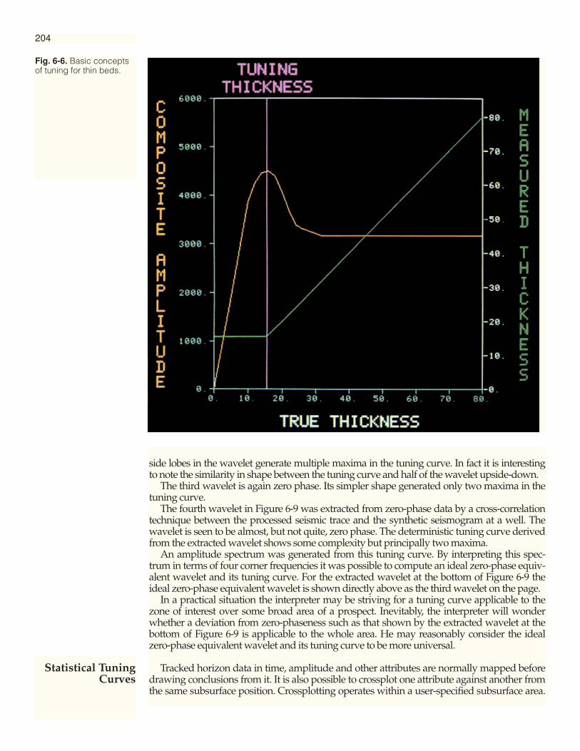
204

side lobes in the wavelet generate multiple maxima in the tuning curve. In fact it is interestingto note the similarity in shape between the tuning curve and half of the wavelet upside-down.

The third wavelet is again zero phase. Its simpler shape generated only two maxima in thetuning curve.

The fourth wavelet in Figure 6-9 was extracted from zero-phase data by a cross-correlationtechnique between the processed seismic trace and the synthetic seismogram at a well. Thewavelet is seen to be almost, but not quite, zero phase. The deterministic tuning curve derivedfrom the extracted wavelet shows some complexity but principally two maxima.

An amplitude spectrum was generated from this tuning curve. By interpreting this spec-trum in terms of four corner frequencies it was possible to compute an ideal zero-phase equiv-alent wavelet and its tuning curve. For the extracted wavelet at the bottom of Figure 6-9 theideal zero-phase equivalent wavelet is shown directly above as the third wavelet on the page.

In a practical situation the interpreter may be striving for a tuning curve applicable to thezone of interest over some broad area of a prospect. Inevitably, the interpreter will wonderwhether a deviation from zero-phaseness such as that shown by the extracted wavelet at thebottom of Figure 6-9 is applicable to the whole area. He may reasonably consider the idealzero-phase equivalent wavelet and its tuning curve to be more universal.

Tracked horizon data in time, amplitude and other attributes are normally mapped beforedrawing conclusions from it. It is also possible to crossplot one attribute against another fromthe same subsurface position. Crossplotting operates within a user-specified subsurface area.

Statistical TuningCurves

Fig. 6-6. Basic conceptsof tuning for thin beds.

205

With this capability statistical analysis of horizon data can be an important part of interactiveinterpretation.

In studying the detailed character of bright spots and the tuning phenomena therein, it maybe desirable to make the simplifying assumption that lateral variations in amplitude are dueto lithologic changes in the reservoir or to tuning effects, and not due to changes in the acousticproperties of the embedding media. Figure 6-10 shows a crossplot of the top sand amplitudesagainst the base sand amplitudes for a particular reservoir. The general proportionalitybetween the two as indicated by the extension of the points along the diagonal yellow lineindicates that, to a first approximation, the lateral changes in amplitude do result from lateralchanges within the reservoir rather than in the encasing material.

In pursuing the more quantitative study of reservoirs (Chapter 7), the absolute value sum-mation of top and base reservoir amplitudes accentuates the properties of the reservoir, litho-logic or geometric, relative to those of the encasing material. This absolute value summation isreferred to as composite amplitude. Figure 6-11 shows a crossplot of composite amplitudeagainst gross isochron (that is, measured thickness). These are the parameters for studyingtuning (Figure 6-6), so Figure 6-11 is a statistical approach to the determination of tuningeffects.

The principal maximum in composite amplitude (Figure 6-11) occurs at 16 ms, the tuningthickness. In addition there is a second maximum evident at about 35 ms. The meaning ofthese two maxima in terms of wavelet interaction was explained schematically in Figure 6-7.The first interpretation of a statistical tuning curve from this crossplot is then the envelope ofthe plotted points (Figure 6-12). This is based on the assumption that the highest amplitudepoints all indicate the maximum acoustic response of the interval under study and thereforethat the variable shape of this envelope with isochron indicates geometric effects alone.

The horizontal blue line to the right of Figure 6-12 is the baseline and indicates the maximumuntuned amplitude. The ratio of the amplitude of the tuning maximum to this baseline value iscontrolled by the side lobe levels of the interfering wavelets. On this basis the tuning maxima as

Fig. 6-8. Tuning curves for two zero-phase wavelets showing multipleamplitude maxima (after Kallweit andWood, 1982).Fig. 6-7. Constructive interference of zero-phase

wavelets to produce tuning maxima.

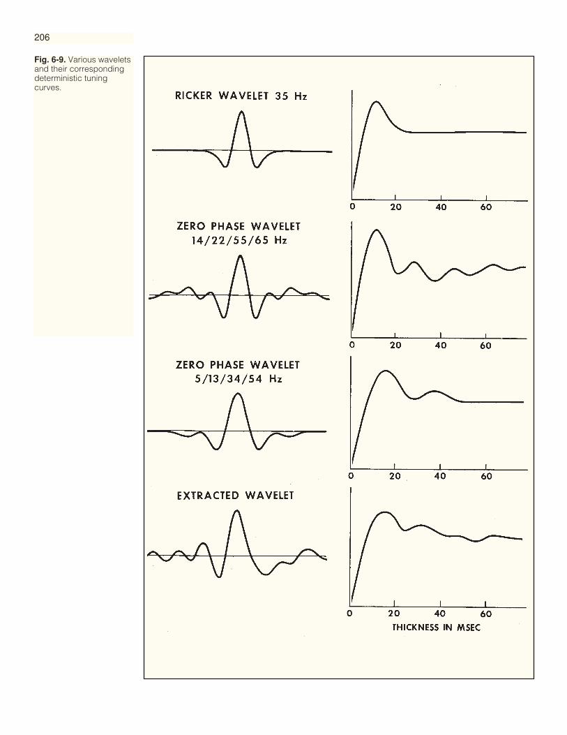
206

Fig. 6-9. Various waveletsand their correspondingdeterministic tuningcurves.

207

drawn in Figure 6-12 are too high. Considering the very large number of points plotted forisochrons in the 10-40 ms range, it is reasonable that some amplitudes are spuriously highbecause of constructive interference of the already-tuned reflections with nonreservoir interfaces,multiples or noise. In Figure 6-13, 99th percentile points computed over 2 ms isochron gates areplotted as blue asterisks. They fall at more reasonable levels relative to the untuned baseline.

Hence the existence of two maxima in the tuning curve was indicated by the raw crossplot,but a statistical analysis of the points guided by the knowledge of the deterministic tuningcurve was required to establish the shape of the final curve. This final interpreted curve isshown in yellow in Figure 6-13.

Figure 6-14 shows the deterministic tuning curve points and the final interpreted curvesuperimposed on the same crossplot. Deterministic tuning curves have arbitrary verticalscales. Hence it was necessary to interpretively judge the factor by which the deterministicpoints must be scaled so that they could be plotted on the same composite amplitude axis asthe crossplot points. This was done by matching the deterministic points to the crossplot enve-lope at the greater thicknesses where little or no tuning effect exists, and was confirmed byplotting the model response at a control well. The yellow curve in Figures 6-13 and 6-14 is thesame. It is repeated to demonstrate how the final interpreted tuning curve for the area understudy tied both the statistical and deterministic inputs.

Interpreters sometimes try to explain as reservoir tuning effects amplitude phenomenawhich really cannot be explained that way. Understanding wavelet shape is the key to under-standing what reasonably can or cannot be interpreted as a tuning effect.

Figure 6-15 shows four zero-phase wavelets of different bandwidths. The lowest frequencyin the band is held the same while the highest frequency is progressively increased by a full

Fig. 6-10. Interactivecrossplot of base sandamplitudes against topsand amplitudesdemonstratingapproximateproportionality.

Understanding theMagnitude ofTuning Effects

208

Fig. 6-11. Interactivecrossplot of compositeamplitude against grossthickness of a reservoirinterval for all theinterpreted data points ina prospect.

Fig. 6-12. Same crossplotas Figure 6-11 with upperenvelope drawn as a firstinterpretation of astatistical tuning curve.

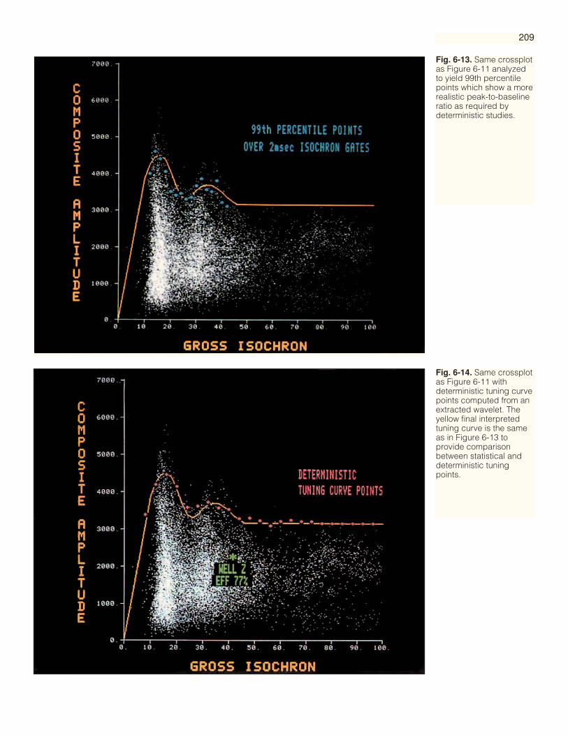
209

Fig. 6-13. Same crossplotas Figure 6-11 analyzedto yield 99th percentilepoints which show a morerealistic peak-to-baselineratio as required bydeterministic studies.

Fig. 6-14. Same crossplotas Figure 6-11 withdeterministic tuning curvepoints computed from anextracted wavelet. Theyellow final interpretedtuning curve is the sameas in Figure 6-13 toprovide comparisonbetween statistical anddeterministic tuningpoints.

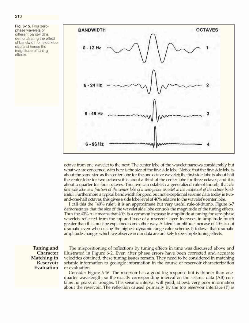
Tuning andCharacter

Matching inReservoir

Evaluation

octave from one wavelet to the next. The center lobe of the wavelet narrows considerably butwhat we are concerned with here is the size of the first side lobe. Notice that the first side lobe isabout the same size as the center lobe for the one octave wavelet; the first side lobe is about halfthe center lobe for two octaves; it is about a third of the center lobe for three octaves; and it isabout a quarter for four octaves. Thus we can establish a generalized rule-of-thumb, that thefirst side lobe as a fraction of the center lobe of a zero-phase wavelet is the reciprocal of the octave band-width. Furthermore a typical bandwidth for good but not exceptional seismic data today is two-and-one-half octaves; this gives a side lobe level of 40% relative to the wavelet’s center lobe.

I call this the “40% rule”; it is an approximate but very useful rule-of-thumb. Figure 6-7demonstrates that the size of the wavelet side lobe controls the magnitude of the tuning effects.Thus the 40% rule means that 40% is a common increase in amplitude at tuning for zero-phasewavelets reflected from the top and base of a reservoir layer. Increases in amplitude muchgreater than this must be explained some other way. A lateral amplitude increase of 40% is notdramatic even when using the highest dynamic range color scheme. It follows that dramaticamplitude changes which we observe in our data are unlikely to be simple tuning effects.

The mispositioning of reflections by tuning effects in time was discussed above andillustrated in Figure 6-2. Even after phase errors have been corrected and accuratevelocities obtained, these tuning issues remain. They need to be considered in matchingseismic information to geologic information in the course of reservoir characterizationor evaluation.

Consider Figure 6-16. The reservoir has a good log response but is thinner than one-quarter wavelength, so the exactly corresponding interval on the seismic data (AB) con-tains no peaks or troughs. This seismic interval will yield, at best, very poor informationabout the reservoir. The reflection caused primarily by the top reservoir interface (P) is

210

Fig. 6-15. Four zero-phase wavelets ofdifferent bandwidthsdemonstrating the effectof bandwidth on side lobesize and hence themagnitude of tuningeffects.

moved up a few milliseconds by tuning, and the reflection caused primarily by the basereservoir interface (T) is moved down. Crestal reflection points yield more reliable ampli-tudes and attributes than points on the flank of the waveform. Thus the best seismic infor-mation about this reservoir lies at P and T, both out-of-place because of tuning, and this isthe information that should be used. The interpreter should match the seismic response tothe well response on character taking account of this tuning mispositioning.

In general the interpreter should recognize that the best information in amplitude andother attributes lies on the waveform crest. Thus, to a first approximation, the number ofreflections dictates the number of reservoir units that may be characterized. If two reser-voir units lie within the same quarter wavelength, then those two units should be studiedtogether as one. Seismic reservoir studies need to be guided by the resolution of the data.Even with excellent data the analysis of one reservoir unit per reflection is probably thebest we can hope to do.

211

Fig. 6-16. Poroussand, with or withouthydrocarbons,typically has a sonicor impedance logsimilar to that on left.Correspondingseismic response inEuropean polarity isshown on right. Theamplitudes thatshould be used tocharacterize thisreservoir are to befound at P and T, andnot over the directlycorrespondinginterval AB.

P

A

B

T

Kallweit, R. S., and L. C. Wood, 1982, The limits of resolution of zero-phase wavelets: Geo-physics, v. 47, p. 1035-1046.

Meckel, L. D., Jr., and A. K. Nath, 1977, Geologic considerations for stratigraphic modelingand interpretation, in C. E. Payton, ed., Seismic stratigraphy — applications to hydrocar-bon exploration: AAPG Memoir 26, p. 417-438.

Neidell, N. S., and E. Poggiagliolmi, 1977, Stratigraphic modeling and interpretation —geophysical principles and techniques, in C. E. Payton, ed., Seismic Stratigraphy —applications to hydrocarbon exploration: AAPG Memoir 26, p. 389-416.

Robertson, J. D., and H. H. Nogami, 1984, Complex seismic trace analysis of thin beds:Geophysics, v. 49, p. 344-352.

Widess, M. B., 1973, How thin is a thin bed?: Geophysics, v. 38, p. 1176-1180.

212

References

213

Reservoir PropertiesDeducible fromSeismic Data

CHAPTER SEVEN

StructureReservoir boundariesFluid content & contactsPorosityHydrocarbon saturationNet pay or net sandPermeabilityConnectivity / flow unitsAquifer / drive mechanismsHeterogeneities

Generally yesGenerally yesYes for younger rocksGenerally yesDifficult but possible for younger rocksGenerally yesNoSometimesPartially yes

all with resolution limitations

WILL 3-D SEISMIC PROVIDE ?RESERVOIR INFORMATION NEEDED Fig. 7-1. Reservoirinformation needed foreffective exploitation andthe generalized ability of3-D seismic data to helpin providing it.

Reservoir EvaluationReservoir evaluation, reservoir characterization or reservoir property mapping is

an important use of 3-D seismic data. As presented here it is an extension of reservoirreflection identification (Chapter 5), horizon slicing techniques (Chapter 4) and tuningphenomena (Chapter 6). Further issues on reservoir evaluation follow in Chapter 8.

Figure 7-1 gives a summary list of reservoir properties needed for effective devel-opment and production of hydrocarbon reserves. The basic information in seismicdata is only time, amplitude and perhaps frequency, so there are many fewer mea-surements than there are unknowns. Seismic attributes (Chapter 8) may be helpfulbut they are not new additional information. Seismic traveltime addresses structureand structural boundaries. Amplitude and frequency are left to address the otherproperties. Amplitude is well understood and is used widely; frequency is less wellunderstood and tends to be noisy.

The principal reservoir properties that affect seismic amplitude can be divided intotwo groups:

GROUP A GROUP Bnature of fluid porositygross lithology net pay thickness or net-to-gross ratio

pressure lithologic detailtemperature hydrocarbon saturation

The properties in Group A are those which, to a first approximation, affect thereservoir as a whole. The difference between gas and oil was discussed in Chapter 5.The gross lithology of a reservoir rock generally does not change much within one

214

Fig. 7-4. Structural shapeof the Macae calcarenitereservoir, Pampo oil field,offshore Brazil. (CourtesyPetroleo Brasileiro.)

NET-TO-GROSS

HC SATURATION

AMPLITUDE

AMPLITUDEDIM SPOT REGIMEHIGH IMPEDANCE RESERVOIR

(low impedance )(reservoir layers)

ACOUSTICIMPEDANCE

PO ROS ITYBRIGHT SPOT REGIMELOW IMPEDANCE RESERVOIR

Fig. 7-3. Explanation ofbright spot and dim spotregimes. In bright spotregime high amplitude isdesirable; in dim spotregime low amplitude isdesirable.

Fig. 7-2. Amplitude varies nonlinearly with hydrocarbonsaturation, particularlyfor gas (Domenico,1974).

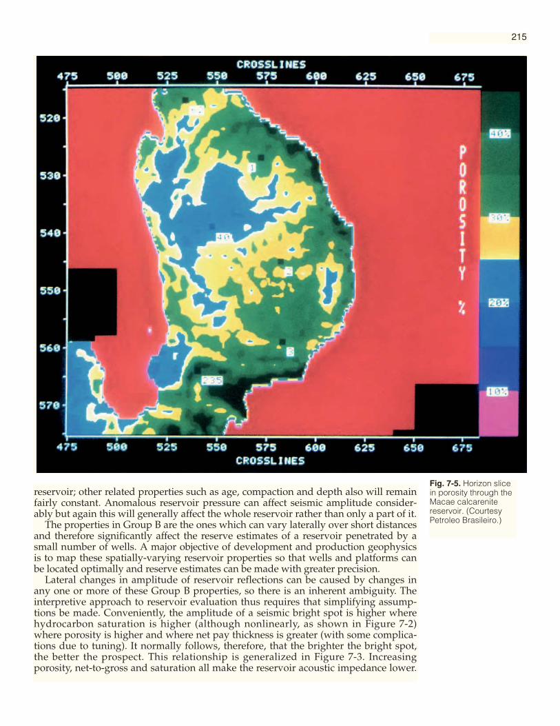
215

reservoir; other related properties such as age, compaction and depth also will remainfairly constant. Anomalous reservoir pressure can affect seismic amplitude consider-ably but again this will generally affect the whole reservoir rather than only a part of it.

The properties in Group B are the ones which can vary laterally over short distancesand therefore significantly affect the reserve estimates of a reservoir penetrated by asmall number of wells. A major objective of development and production geophysicsis to map these spatially-varying reservoir properties so that wells and platforms canbe located optimally and reserve estimates can be made with greater precision.

Lateral changes in amplitude of reservoir reflections can be caused by changes inany one or more of these Group B properties, so there is an inherent ambiguity. Theinterpretive approach to reservoir evaluation thus requires that simplifying assump-tions be made. Conveniently, the amplitude of a seismic bright spot is higher wherehydrocarbon saturation is higher (although nonlinearly, as shown in Figure 7-2)where porosity is higher and where net pay thickness is greater (with some complica-tions due to tuning). It normally follows, therefore, that the brighter the bright spot,the better the prospect. This relationship is generalized in Figure 7-3. Increasingporosity, net-to-gross and saturation all make the reservoir acoustic impedance lower.

Fig. 7-5. Horizon slicein porosity through theMacae calcarenitereservoir. (CourtesyPetroleo Brasileiro.)

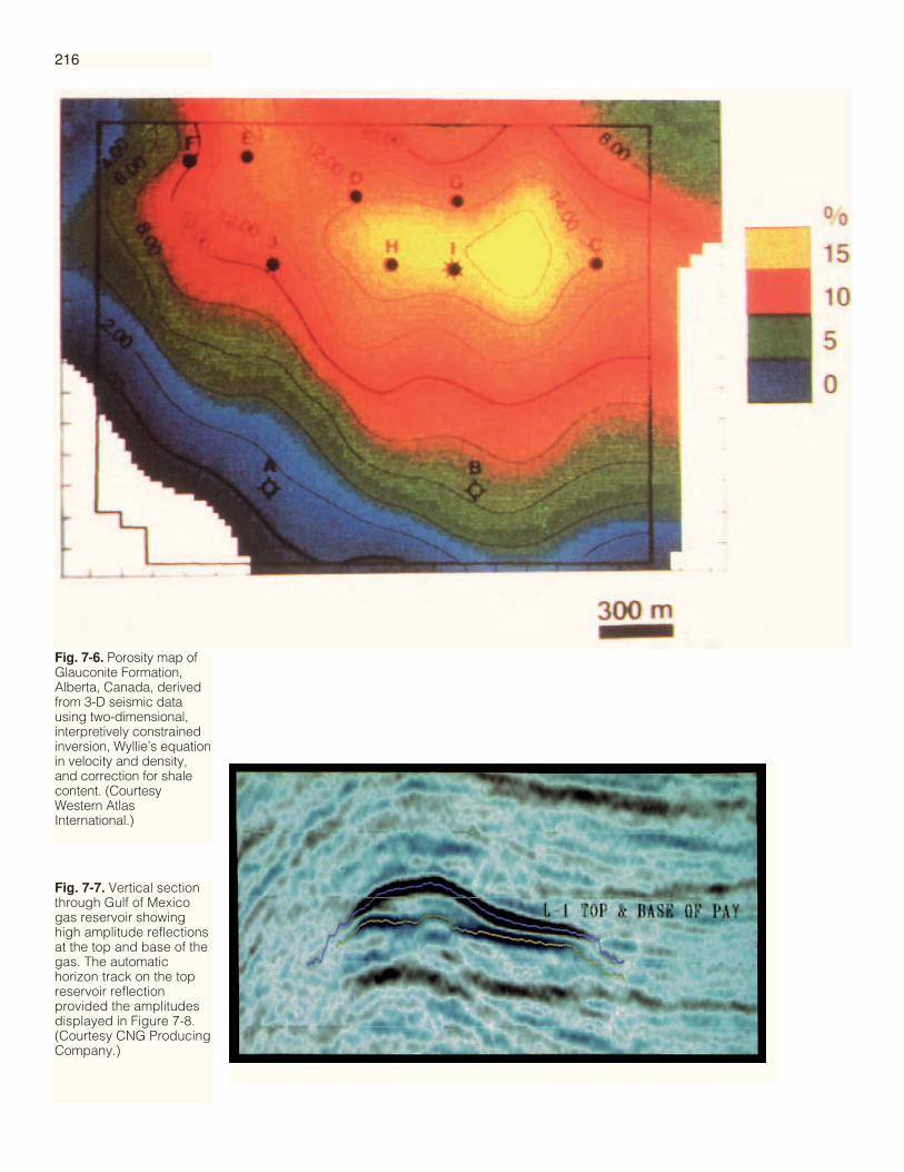
216

Fig. 7-7. Vertical sectionthrough Gulf of Mexicogas reservoir showinghigh amplitude reflectionsat the top and base of thegas. The automatichorizon track on the topreservoir reflectionprovided the amplitudesdisplayed in Figure 7-8.(Courtesy CNG ProducingCompany.)

Fig. 7-6. Porosity map ofGlauconite Formation,Alberta, Canada, derivedfrom 3-D seismic datausing two-dimensional,interpretively constrainedinversion, Wyllie’s equationin velocity and density,and correction for shalecontent. (CourtesyWestern AtlasInternational.)

217

The reservoir “sweet spots” are thus the low-impedance areas. In the bright spotregime the amplitude of the reservoir reflections is then higher. This includes hydro-carbon bright spots but is not limited to them — any already low impedance reservoirwill get lower and thus generate more amplitude. In the dim spot regime the reverseoccurs. Here the reservoir is higher acoustic impedance than the embedding medium,so reducing impedance reduces contrast and thus amplitude. Clearly the most impor-tant seismic property of a reservoir is whether it is bright spot or dim spot regime. Inthe former, high amplitude is good and the distribution of amplitude on the horizonslice guides development drilling (e.g., Figures 2-31 to 2-33). The reservoirs discussedin this chapter are in the bright spot regime. Case history 12 (Chapter 9) discusses adim spot regime reservoir and another good example is illustrated in Figure 4-51.

Figure 7-4 shows the structural configuration of the Macae calcarenite reservoir inthe Pampo oil field offshore Brazil (Curtis, Martinez, Possato, Saito, 1983). Amplitudevariations of the calcarenite event were considered to result primarily from porositychanges within the reservoir. The 3-D data volume was processed through recursiveseismic inversion. The low-frequency interval velocity field originated from a 3-Dinverse normal-incidence ray tracing procedure. The resultant velocities in the reser-voir were then converted to apparent porosity using Wyllie’s equation (Wyllie, Grego-ry, and Gardner, 1958). Figure 7-5 shows a horizon slice through the Macae calcarenite

Fig. 7-8. Horizon slice fromGulf of Mexico Pleistocenegas reservoir showingpatterns in amplitudeinterpretable as the effectsof hydrocarbon, faulting,porosity, and tuning.Yellow bar is one km. Redlines indicate the positionof vertical section in Figure7-7. Black line is blockboundary. (Courtesy CNGProducing Company.)

Porosity UsingInversion

218

displaying apparent porosity variations within the reservoir. A decrease in porositytoward the reservoir core is evident and is confirmed by well data.

Some kind of seismic inversion may be considered useful when attempting to bequantitative about reservoir properties. The conversion from interface information(normal seismic amplitudes) to interval information (inverted seismic amplitudes)brings the seismic data into a more geologic form, one more readily correlated to welllogs and to reservoir properties, but is highly dependent on a proper understanding ofdata phase and polarity.

In the project leading to the porosity map of Figure 7-6, 3-D seismic data wereinverted by a two-dimensional inversion process where the bandwidth was effective-ly broadened by interpretive constraint. The resultant data were in acousticimpedance and well data were available in velocity and density. Wyllie’s equations invelocity and density were thus combined together. Both of these versions consider theaddition of components of a mixture of sand grains, shale and hydrocarbon in porosi-ty; the densities add up directly and the velocities add up as their inverse, namelytransit time. The shale volume corrections were obtained from the well control. Fol-lowing this procedure, the reservoir porosity map of Figure 7-6 was obtained. It wasused to predict successfully the porosity at two later wells.

Further porosity mapping projects are described in Case Histories 6 and 12 (Chapter 9).

A horizon slice showing the spatial distribution of seismic amplitude over a reser-voir top or base is an enormously valuable aid for studying that reservoir. The value

Fig. 7-9. Structure map ofproductive Gulf of Mexicosand showing setting insalt dome prospect.(Courtesy Chevron U.S.A.Inc.)

Horizon Slices OverReservoir Interfaces

219

comes not only from spatial continuity but also from the faithful amplitude recon-struction resulting from 3-D migration. For a low acoustic impedance reservoir, highamplitude is good because it may be caused by higher net-to-gross ratio, higherporosity, or higher hydrocarbon saturation.

Figure 7-7 shows high-amplitude reflections from a Pleistocene gas reservoir.The red reflection is from the reservoir top and the blue reflection is from the fluidcontact. The horizon slice in Figure 7-8 follows the maximum amplitude of the topreflection. The overall high-amplitude triangular shape indicates the extent of thegas. Along the northern dip-controlled boundary, the amplitude gradient can beextrapolated to find the actual downdip reservoir limit. Some internal roughlynortheasterly lineations indicate faulting. A high-amplitude trend running N60˚Eand crossing from the high amplitude gas area into the low amplitude surroundingarea in the upper right corner is interpreted as a depositional trend of higherporosity. The high-amplitude trend running N80˚W parallel to and just south of thenorthern reservoir boundary is caused by tuning. Separation of different effects inthis way on the basis of interlocking patterns should be a normal part of horizonslice interpretation.

Figures 7-9 and 7-10 show a structure map and horizon slice from another Gulf ofMexico field. Again, different effects can be interpreted based on their differentamplitude patterns. Salt is to the northwest and gas is trapped against the salt, asindicated in red. Variable porosity in the wet sand is probably responsible for theirregular yellow patterns downdip. The high amplitudes, principally in red, follow-ing the upthrown side of fault A and spanning a structural range of 2,000 feet, can

Fig. 7-10. Horizon slicecorresponding tostructure map of Figure 7-9. The red colors close tothe salt indicate gas. Theyellows indicate aporosity overprint. Thehigh amplitudes along theupthrown side of fault Aare interpreted ashydrocarbons in migrationafter flowing up the fault.(Courtesy Chevron U.S.A.Inc.)

220

only be interpreted as gas actively migrating toward the trap. This same observationand interpretation has been made on serveral other horizon slices in Tertiary clasticbasins, for example Figure 7-11.

In an area of Pleistocene sediments offshore Louisiana the wells indicated thateach reservoir sand interval was composed of several thin productive lobes and thatthe position of these lobes within the sands and their thickness varied laterally overa short distance (Brown, Wright, Burkart, Abriel, 1984). The top and base of the grosssand intervals generate the seismic reflections and the nonproductive segmentswithin them are caused by the sands becoming tight and shaly. The aggregate thick-ness of the productive lobes is what matters economically. Therefore, the overallobjective is to use amplitude measurements, coupled with time thickness measure-ments, to determine the spatial distribution of net producible gas sand from the seis-mic data.

The use of seismic amplitude to measure the proportion of sand within asand/shale interval was demonstrated by Meckel and Nath (1977) for beds less thantuning thickness. Here the principle has been extended to thicker beds on theassumption that the individual lobes of producible gas sand are each below tuningthickness, that producible gas sand is a material of uniform acoustic properties, andthat the internal layering is reasonably uniform.

Figure 7-12 shows bright reflections from one reservoir sand. The single blue-over-red signature indicates zero-phaseness and European polarity (see Chapter 2). Figure7-13 shows two examples of two reservoir sands. Automatic tracking on an interac-

Fig. 7-11. Gulf of Mexicohorizon slice. The high-amplitude lineationsindicate hydrocarbonmigration pathways. Notethat high-amplitudelineations and low-amplitude lineations areboth associated with thefaults. (Courtesy ConocoInc.)

Net Pay Thickness

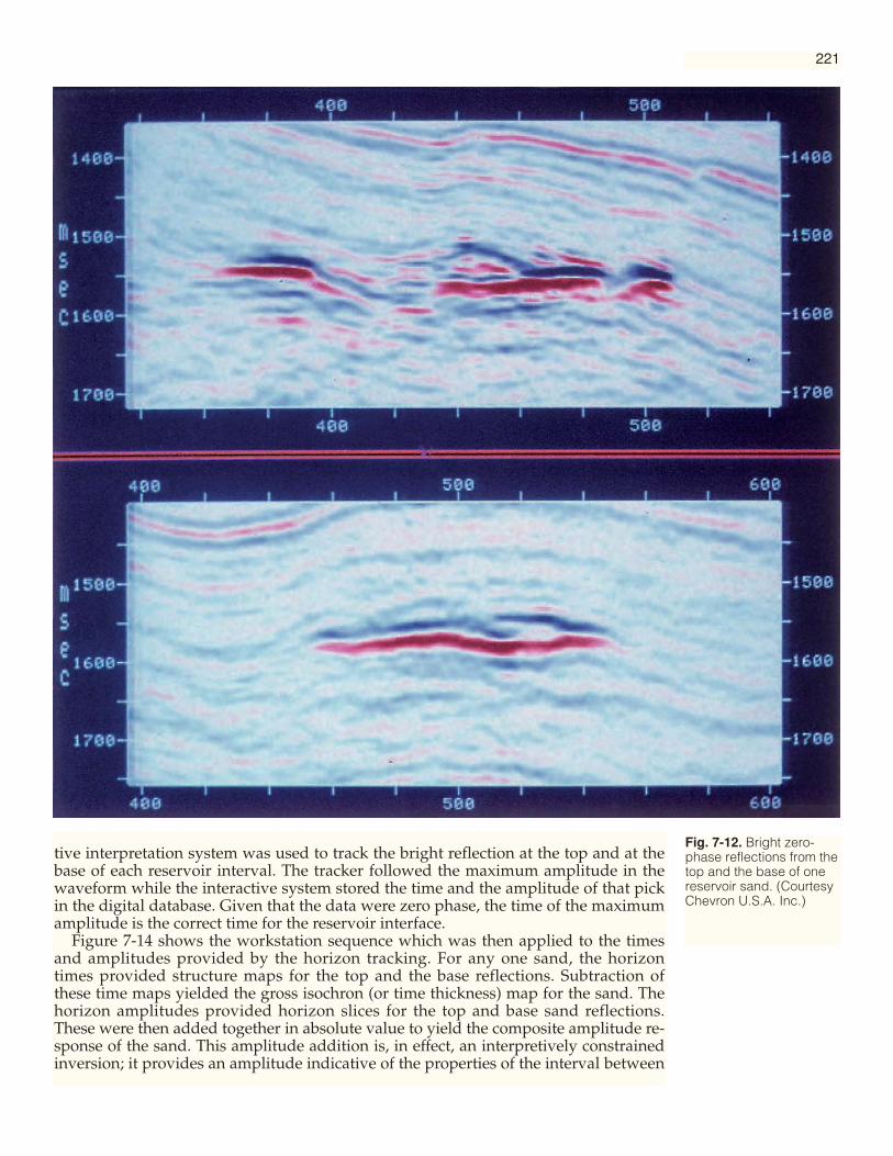
221

Fig. 7-12. Bright zero-phase reflections from thetop and the base of onereservoir sand. (CourtesyChevron U.S.A. Inc.)

tive interpretation system was used to track the bright reflection at the top and at thebase of each reservoir interval. The tracker followed the maximum amplitude in thewaveform while the interactive system stored the time and the amplitude of that pickin the digital database. Given that the data were zero phase, the time of the maximumamplitude is the correct time for the reservoir interface.

Figure 7-14 shows the workstation sequence which was then applied to the timesand amplitudes provided by the horizon tracking. For any one sand, the horizontimes provided structure maps for the top and the base reflections. Subtraction ofthese time maps yielded the gross isochron (or time thickness) map for the sand. Thehorizon amplitudes provided horizon slices for the top and base sand reflections.These were then added together in absolute value to yield the composite amplitude re-sponse of the sand. This amplitude addition is, in effect, an interpretively constrainedinversion; it provides an amplitude indicative of the properties of the interval between

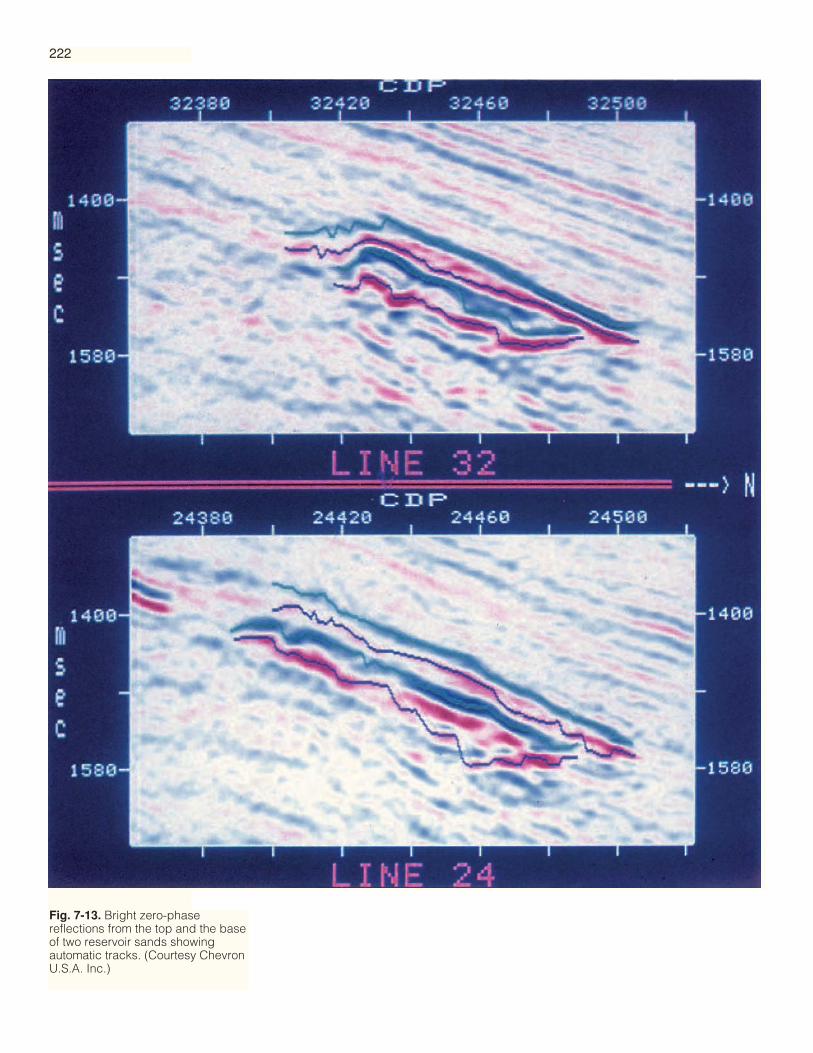
222

Fig. 7-13. Bright zero-phasereflections from the top and the baseof two reservoir sands showingautomatic tracks. (Courtesy ChevronU.S.A. Inc.)

the top and base reservoir reflections, as interpreted. The principle is diagrammed inFigure 7-15.

Tuning effects remain as a distortion in this composite amplitude and should beremoved. The key is to understand the shape of the tuning curve in detail; this can beobtained deterministically from an extracted wavelet or statistically from a crossplot(see Chapter 6). In this offshore Louisiana example both methods were used to yield theyellow tuning curve of Figure 7-16. Editing was then required to change the responsefrom that shown in yellow to that shown in orange (using a multiplicative factor), sothat the amplitude as a function of gross reservoir thickness alone is constant abovetuning thickness and linearly decaying to zero for decreasing thickness below tuning.

In order to conclude the interpretive sequence of Figure 7-14, the composite ampli-tude response was edited according to Figure 7-16, and scaled with a single factorderived from one well to yield a map of net gas/gross sand ratio. Combining this bymultiplication with the gross isochron map, a net gas isochron map was obtained. Aconstant gas sand interval velocity was then sufficient to convert this net gas isochronmap to a net gas isopach map. In combining the gross isochron map with the netgas/gross sand ratio (derived by editing with the function in Figure 7-16), it shouldbe remembered that there are no gross isochrons less than tuning thickness because ofthe tuning phenomenon itself (Figure 6-2). For actual gas sand thicknesses less thantuning, all the net gas sand information is encoded in the amplitude.

Figures 7-17 and 7-18 show comparable gross and net isochron maps, making clearthe contribution of the net gas/gross sand ratio derived from the composite ampli-tude (Figure 7-19). Note the two northwest-southeast thickness trends on the grossisochron map and then note that only one of them has survived in the net isochronmap. This is caused directly by the higher amplitudes to the north and east as seen inFigure 7-19. Net gas sand maps derived in this way have been shown to tie well dataacceptably. In practice, relative values are more accurate than absolute values becauseof the difficulty of determining the scale factor connecting edited amplitude to netgas/gross sand ratio.

When there is more than one mappable reservoir interval associated with the reser-voir under study, each interval is treated separately and added together at net gasisopach stage. Figure 7-20 shows total net producible gas sand in color superimposedon the structural configuration of the top of the reservoir. Integration of net gasisopach maps yields the volume of the reservoir. By integrating over chosen sub-areas, the reservoir volume over different lease blocks or areas of special interest canbe readily determined.

Case Histories 7 and 11 (Chapter 9) report on the use of net gas sand mapping inother prospects. Different approaches to mapping net pay have been presented byWoock and Kin (1987) and by McCarthy (1984).

Text continues on page 230

223

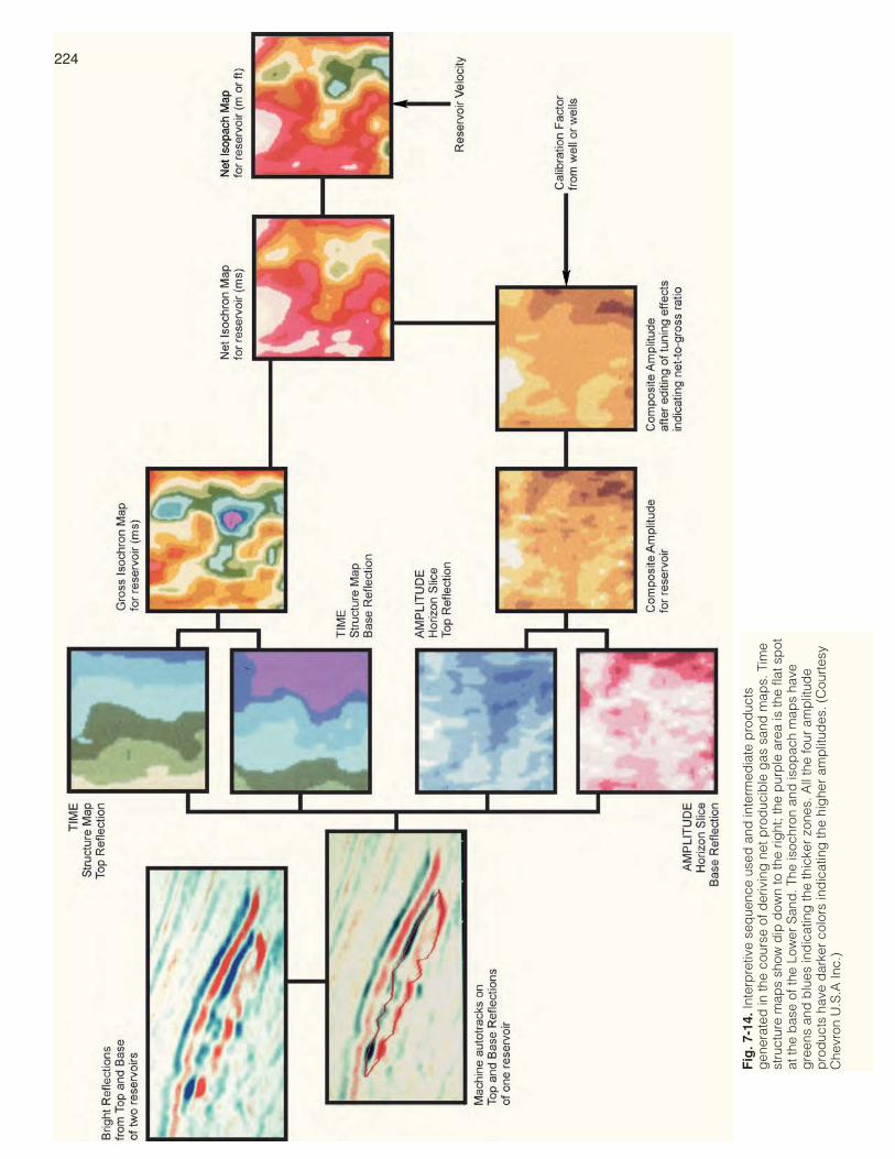
224

Fig

. 7-1

4.In

terp

retiv

e se

que

nce

used

and

inte

rmed

iate

pro

duc

tsg

ener

ated

in th

e co

urse

of d

eriv

ing

net

pro

duc

ible

gas

san

d m

aps.

Tim

est

ruct

ure

map

s sh

ow d

ip d

own

to th

e rig

ht; t

he p

urp

le a

rea

is th

e fla

t sp

otat

the

bas

e of

the

Low

er S

and

. The

isoc

hron

and

isop

ach

map

s ha

veg

reen

s an

d b

lues

ind

icat

ing

the

thic

ker

zone

s. A

ll th

e fo

ur a

mp

litud

ep

rod

ucts

hav

e d

arke

r co

lors

ind

icat

ing

the

hig

her

amp

litud

es. (

Cou

rtes

yC

hevr

on U

.S.A

Inc.

)

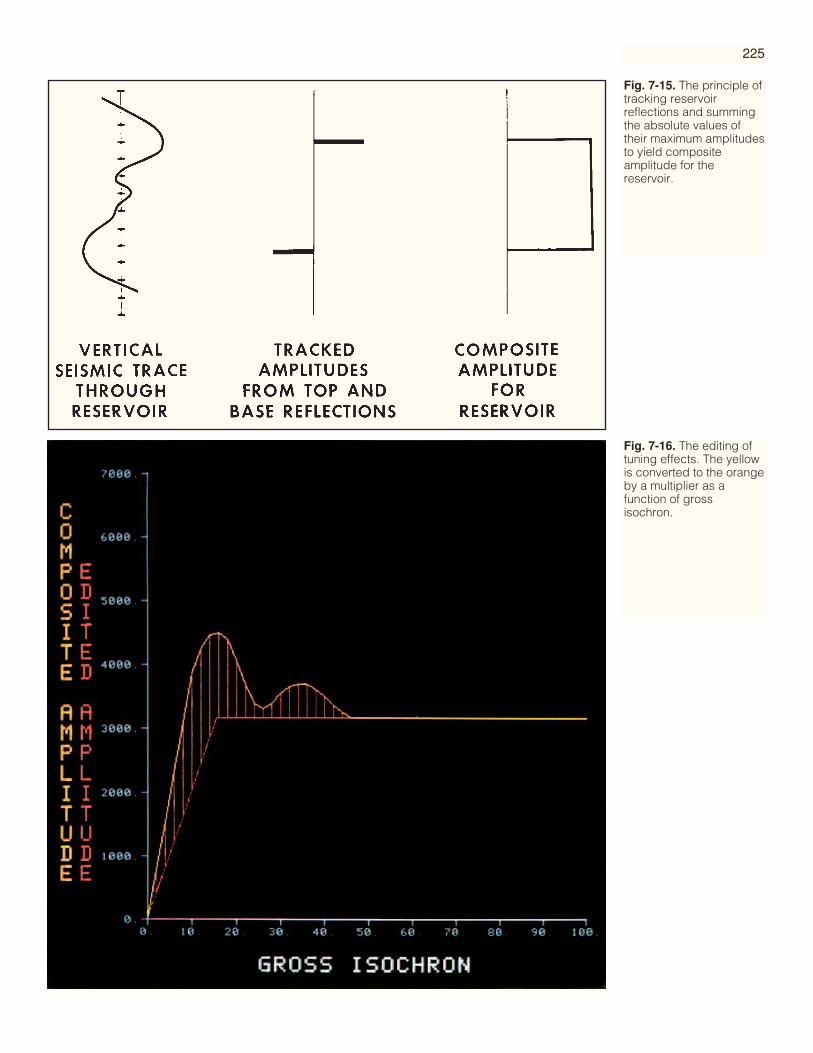
225

Fig. 7-15. The principle oftracking reservoirreflections and summingthe absolute values oftheir maximum amplitudesto yield compositeamplitude for thereservoir.

Fig. 7-16. The editing oftuning effects. The yellowis converted to the orangeby a multiplier as afunction of grossisochron.

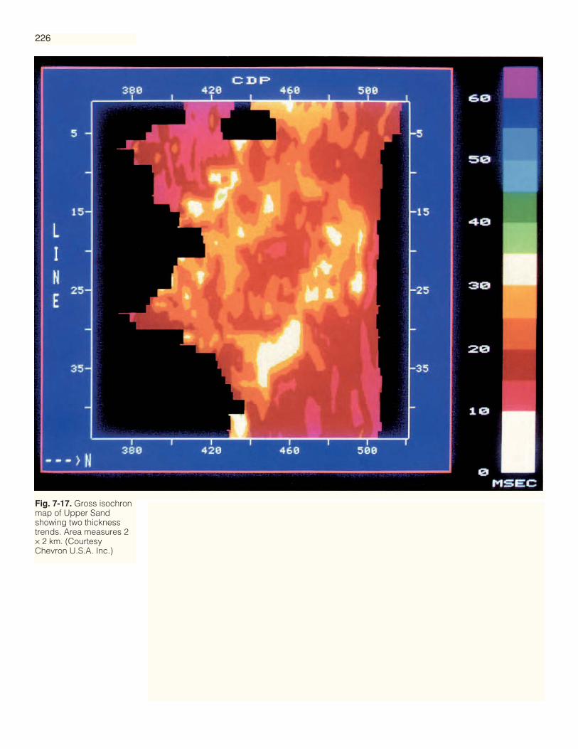
226

Fig. 7-17. Gross isochronmap of Upper Sandshowing two thicknesstrends. Area measures 2× 2 km. (CourtesyChevron U.S.A. Inc.)

227

Fig. 7-18. Net gasisochron map of UpperSand showing onethickness trend. (CourtesyChevron U.S.A. Inc.)

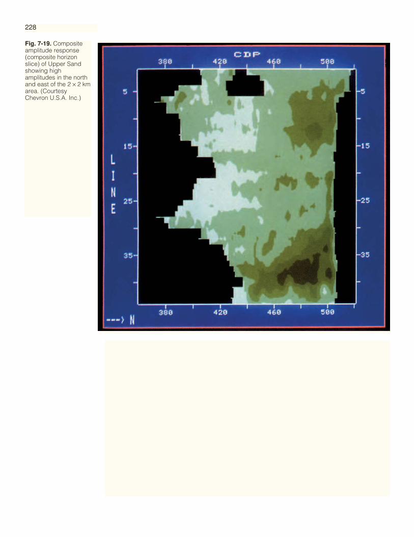
228

Fig. 7-19. Compositeamplitude response(composite horizonslice) of Upper Sandshowing highamplitudes in the northand east of the 2 × 2 kmarea. (CourtesyChevron U.S.A. Inc.)

229

Fig. 7-20. Total net gassand isopach mapsuperimposed on thestructure of the top of thereservoir. The greens andblues indicate the thickernet gas zones. (CourtesyChevron U.S.A. Inc.)

In the above method, porosity was constant and therefore was not discussed. Ingeneral for the bright spot regime, porosity multiplies with net pay thickness to giveporosity-thickness or pore volume. So the general statement of the method becomes:PORE VOLUME = AMPLITUDE � ISOCHRON. This is illustrated further in Figure7-21. Composite amplitude with tuning effects edited is normally the best amplitudeto use. However, single horizon amplitude or windowed amplitude, with or withoutdetuning, are all alternatives. Many variations have been tried and successes report-ed. For example, Neff (1990) starts with a modeled response at a well and thusattempts to handle vertical non-uniformity in the reservoir. Matteucci (1996) triedmany seismic attributes and concluded that the composite amplitude-isochron prod-uct is “the attribute most strongly related to hydrocarbon pore volume.”

Another way of viewing the benefit of the amplitude-isochron product is that itcombines regions where the thickness is below quarter-wavelength and regionswhere it is above into a single reservoir thickness map. For dim spot regime res-ervoirs, the good reservoir quality regions exhibit low amplitude. For this type ofreservoir, the general relation becomes: PORE VOLUME = ISOCHRON ÷ AMPLITUDE.

Consider the following exploration or development problem: We have mapped thereservoir isopach thick at one location; we have mapped the reservoir amplitudemaximum at another location; and we have mapped the structural high at a thirdlocation. Which should we drill? The answer is “none of the above.” We should multi-ply the isopach by the amplitude and drill the location of the product maximum.

Seismic amplitude or other attributes extracted over one reservoir reflection fromgood quality data has high relative accuracy. However, it has no absolute accuracyand calibration with well data is necessary. There are many approaches and these aresummarized in Figure 7-22. The author has had greatest success with the determinis-

Fig. 7-21. Reflectionamplitude, preferablycomposite of reservoir topand base, times isochronthickness is normally thebest measure of reservoirpore volume.

230

porosity thickness time interval

x VELOCITY

x CALIBRATION FACTOR

For bright spot regime:

PORE VOLUME = AMPLITUDE x ISOCHRON

Base

Top

Compositeamplitudexisochron

compositesingle horizondetunedwindowed

Pore Volume

Well Calibration

tic method using a single space-invariant scale factor. This factor can be determinedfrom one well, where the amplitude is highest and the tie most reliable, from twowells, or from a crossplot using many wells. The single factor retains the relativities inthe seismic data, its greatest strength.

If other properties of the reservoir and adjacent layers affect amplitude significant-ly and vary spatially, a space-variant scale factor, determined from the wells, will benecessary to remove them. A good discussion of secondary factors affecting ampli-tude and their removal appears in Case History 12. In projects like this one the rela-tivities in the seismic amplitude are being changed by the different well ties. In gener-al the uncertainties in the position of each well and its measured property need to beconsidered, and also the uncertainties in the seismic measurement. The tie in thedesired reservoir property between the seismic value and the well value needs only tobe within each other’s uncertainty and thus distortion of seismic relativities or flexingcan be minimized.

In geostatistical approaches to well calibration (Figure 7-22) several reservoir prop-erty maps may be desired and several seismic attributes may be considered as a sourceof information. Crossplots establish relationships and variograms guide the spatialinterpolation or cokriging. However, good statistical correlations are not sufficient forreliable extraction of multiple reservoir property maps; support from petrophysics andmodeling is also required. Matteucci (1996) summed up this situation nicely: “It is verysimple and easy to find relationships. It is much harder to estimate if they are statisti-cally significant, robust, and geologically meaningful.” Use of various attributes andmultiple attributes in reservoir studies is discussed further in Chapter 8.

Once the time and amplitude of the zero-phase reflections from the top and base ofa reservoir are stored in a readily-accessible digital database, statistical studies of thehorizon data are straightforward. The value of interactive crossplotting for the statis-tical analysis of tuning phenomena was explained in Chapter 6.

Fig. 7-22. Methods ofcalibration of seismicamplitude or otherattribute to reservoirproperties at wells. Tieshould minimize seismicflexing to fit well valuewithin uncertainties.

231

Calibrate toone or two wells

(single scale factor)

DETERMINISTIC GEOSTATISTICAL

Calibrate to multiple wells

Crossplots andvariograms

for relationships

Maps of severalreservoir properties

Map of one principalreservoir property

Map of one principalreservoir property

Retains relativitiesof seismic data

Variations in otherreservoir propertiesless than uncertainties

Removes variationsin other reservoirproperties

Depends entirely onreliability ofwell measurements

Depends entirely onreliability ofwell measurements

INTERMEDIATE

Attribute is cokrigedwith well-measuredreservoir properties

SINGLE SCALE FACTORSPACE-VARIANT SCALING

Petrophysicsand modeling

for understanding

Statistical Use ofTracked HorizonData

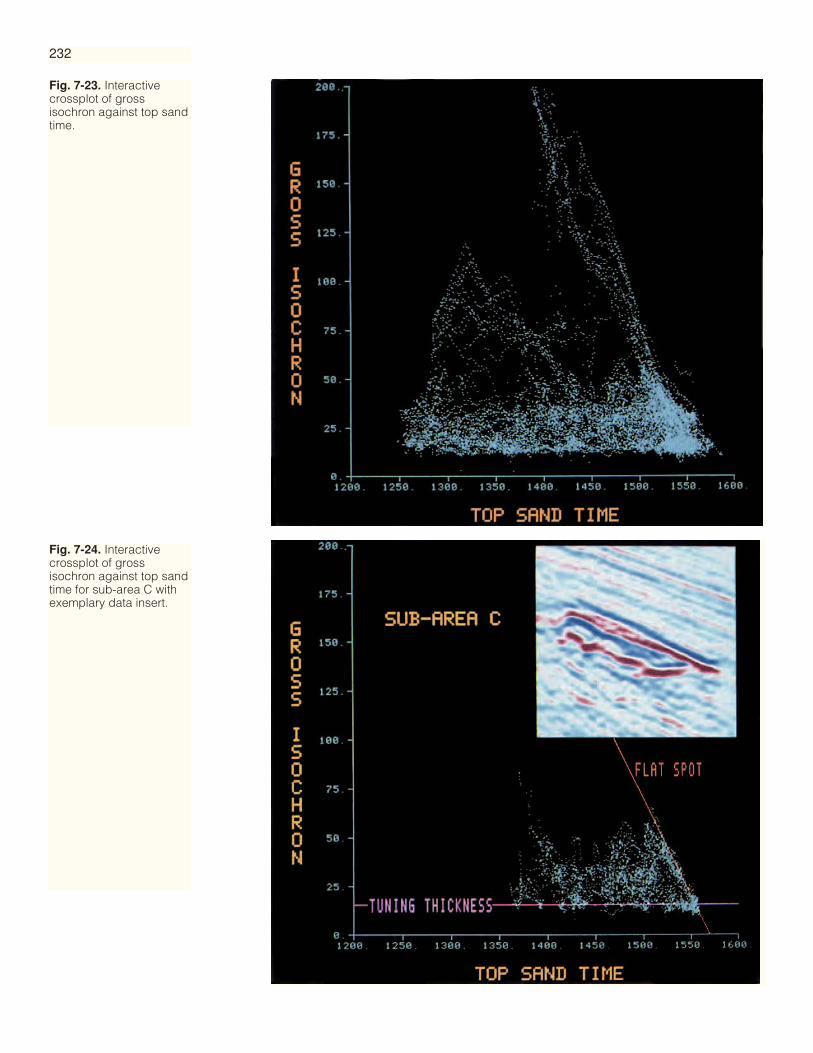
232

Fig. 7-23. Interactivecrossplot of grossisochron against top sandtime.

Fig. 7-24. Interactivecrossplot of grossisochron against top sandtime for sub-area C withexemplary data insert.

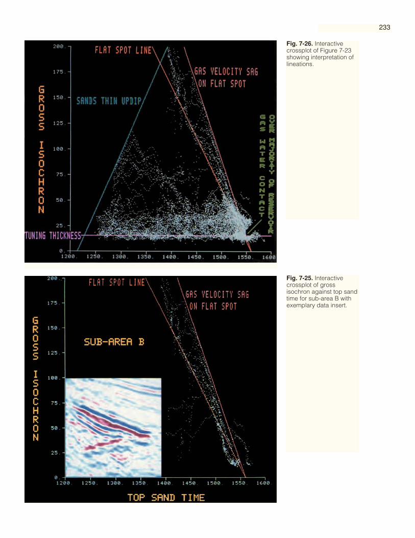
233

Fig. 7-25. Interactivecrossplot of grossisochron against top sandtime for sub-area B withexemplary data insert.

Fig. 7-26. Interactivecrossplot of Figure 7-23showing interpretation oflineations.

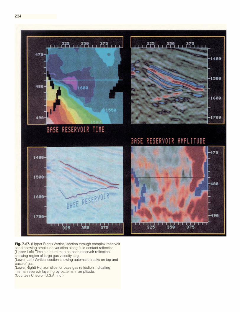
234

Fig. 7-27. (Upper Right) Vertical section through complex reservoirsand showing amplitude variation along fluid contact reflection.(Upper Left) Time structure map on base reservoir reflectionshowing region of large gas velocity sag.(Lower Left) Vertical section showing automatic tracks on top andbase of gas.(Lower Right) Horizon slice for base gas reflection indicatinginternal reservoir layering by patterns in amplitude.(Courtesy Chevron U.S.A. Inc.)

235

Fig. 7-28. Vertical sectionfrom Gulf of Mexicoshowing thick gasreservoir filled with stronginternal reflections.(Courtesy Chevron U.S.A.Inc.)

Fig. 7-29. Macro-layers ofhigh and mediumeffectiveness (net-to-gross ratio) caused bymicro-layers of gas sandinterbedded with shale.

Figure 7-23 shows an interactive crossplot of gross isochron against top sand time;that is, vertical thickness (in time) against structural position. The general effect is tri-angular with several clearly visible lineations. Interpretation of these lineations is astatistical assessment of the many thousands of data points included in this crossplot.Figures 7-24 and 7-25 are crossplots of sub-areas of the prospect, each accompaniedby an exemplary data segment. Figure 7-24 makes it clear that the lineation along thebottom of the crossplot illustrates that thicknesses can only be measured down to justbelow tuning.

Sub-area C (Figure 7-24) includes many lines of data illustrating good flat spotreflections, one of which is illustrated in the data insert. The orange straight linelabelled FLAT SPOT is a line of the form, y = c – x, that is, one representing equalincrements of gross isochron and top sand time. Because top sand time plus grossisochron equals base sand time and because base sand time is approximately constant

236

Fig. 7-30. Horizon slice invelocity through VivianPay Sand showing lowvelocity zone enclosingthe area of producingwells. (CourtesyOccidental Explorationand ProductionCompany.)

237

Fig. 7-31. Fault planecontour map, used as thereference surface for faultslicing. (Courtesy TexacoU.S.A. Inc.)

238

Fig. 7-32. Fault slice through Gulf of Mexico data volumeparallel to the major growth fault mapped in Figure 7-31.Horizon tracks show deep structure caused by saltmovement. (Courtesy Texaco U.S.A. Inc.)

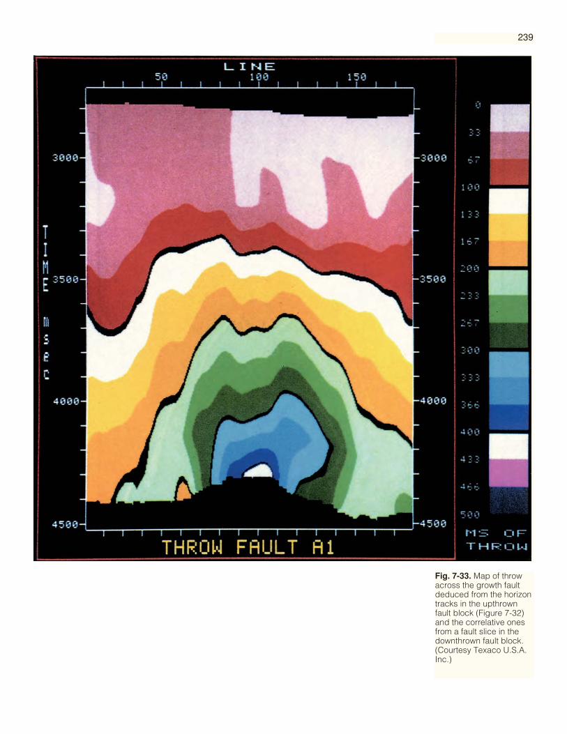
239

Fig. 7-33. Map of throwacross the growth faultdeduced from the horizontracks in the upthrownfault block (Figure 7-32)and the correlative onesfrom a fault slice in thedownthrown fault block.(Courtesy Texaco U.S.A.Inc.)

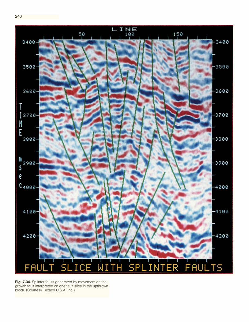
240

Fig. 7-34. Splinter faults generated by movement on thegrowth fault interpreted on one fault slice in the upthrownblock. (Courtesy Texaco U.S.A. Inc.)

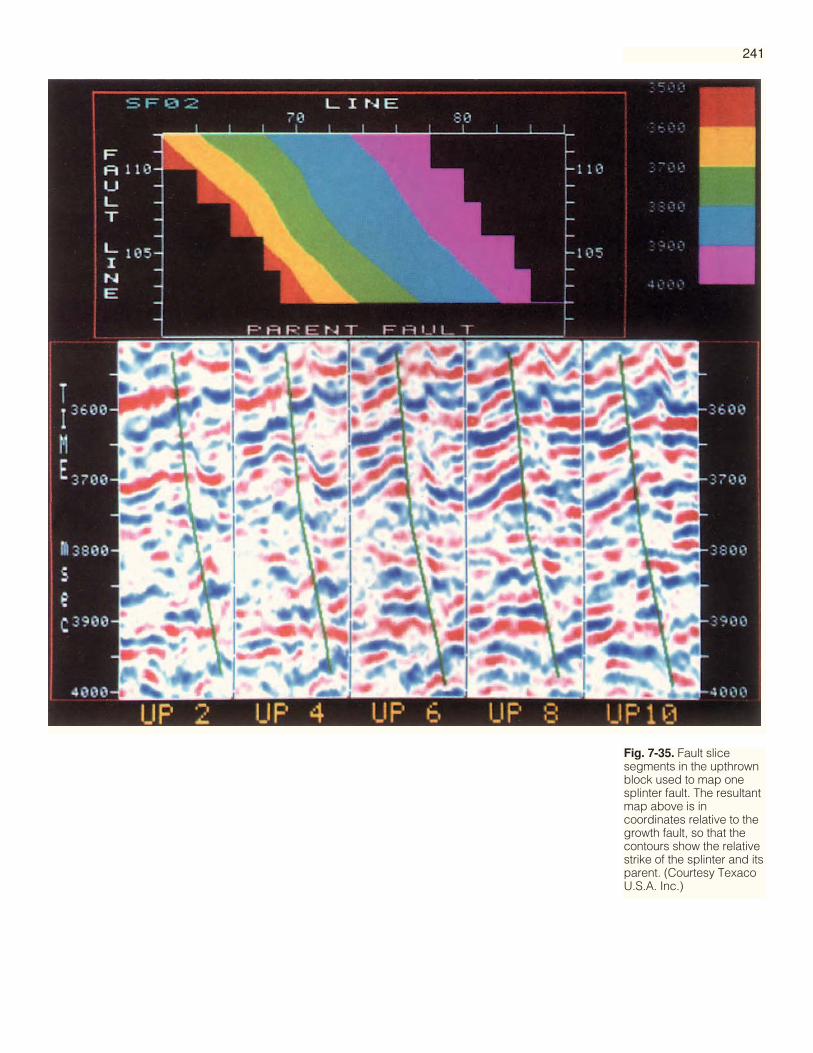
241

Fig. 7-35. Fault slicesegments in the upthrownblock used to map onesplinter fault. The resultantmap above is incoordinates relative to thegrowth fault, so that thecontours show the relativestrike of the splinter and itsparent. (Courtesy TexacoU.S.A. Inc.)

242

Fig

. 7-3

6.U

nrol

led

faul

t slic

e in

dep

th a

long

faul

t pla

ne fr

omN

iger

ia. I

nter

pre

tatio

n of

san

ds

and

sha

les

tied

to th

ree

wel

lsw

as fo

r th

e st

udy

of fa

ult s

ealin

g (

Bou

vier

et a

l., 1

989,

ref

eren

cein

Cha

pte

r 8)

. (C

ourt

esy

Kon

inkl

ijke/

She

ll.)

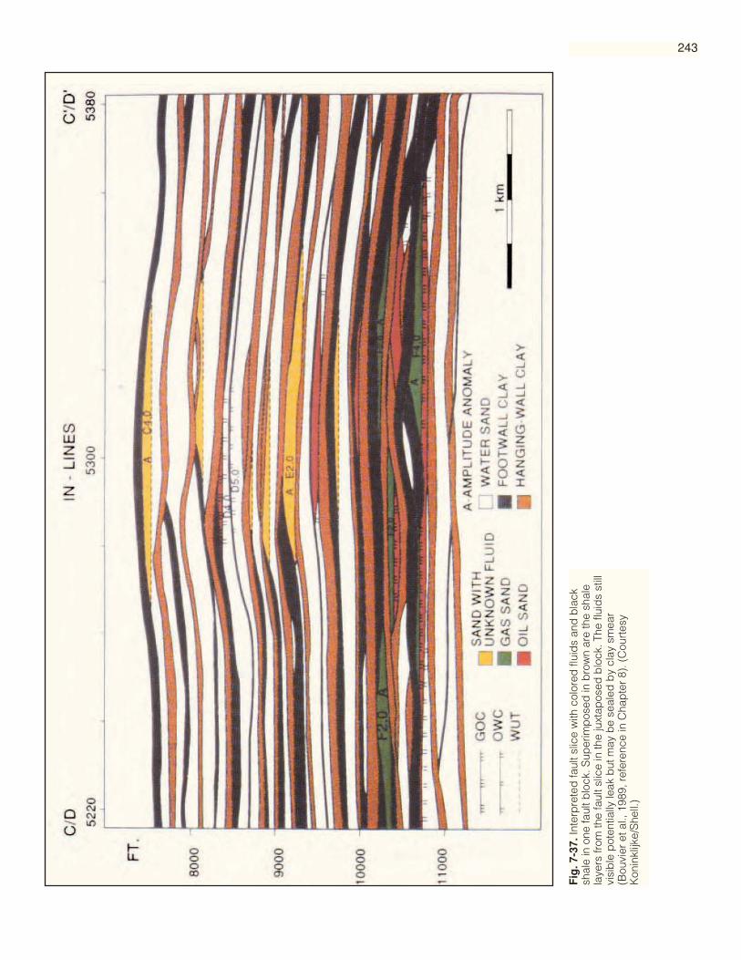
243

Fig

. 7-3

7.In

terp

rete

d fa

ult s

lice

with

col

ored

flui

ds

and

bla

cksh

ale

in o

ne fa

ult b

lock

. Sup

erim

pos

ed in

bro

wn

are

the

shal

ela

yers

from

the

faul

t slic

e in

the

juxt

apos

ed b

lock

. The

flui

ds

still

visi

ble

pot

entia

lly le

ak b

ut m

ay b

e se

aled

by

clay

sm

ear

(Bou

vier

et a

l., 1

989,

ref

eren

ce in

Cha

pte

r 8)

. (C

ourt

esy

Kon

inkl

ijke/

She

ll.)

244

for a flat spot reflection, it is indeed expected that a flat spot would plot along such adiagonal line of unit gradient.

Sub-area B (Figure 7-25) is an area of thicker sands. An orange line represents theline of equal increments of gross isochron and top sand time as before. Most of thepoints fall to the right of this line, indicating varying degrees of gas velocity sag.Extreme sag is illustrated in the data insert and marked on the crossplot by a pink line.

An interpreted version of the total area crossplot of Figure 7-23 is shown in Figure 7-26. This interpretation incorporates the observations from several sub-areas including thetwo discussed here. The convergence of many of the lineations in the lower right cornerand also the great concentration of crossplot points at the same location suggest a com-mon gas/water contact over a large part of the reservoir. This in turn suggests that muchof the reservoir is in communication, at least in terms of flow rates effective over geologictime. The concentration of points in a swath along the lower part of the triangular pat-tern suggests that many of the sands were preferentially deposited with thicknesses of 30ms (approximately 25 m) or less.

There is a suggestion of a lineation with the correct slope to be another flat spotreflection intersecting the top sand time axis at 1,440 ms. It is evident on both Figures7-26 and 7-24. This observation can be considered to be the statistical identification ofanother possible fluid contact, which has obvious implications for segmentation of thereservoir.

Figure 7-27 illustrates several aspects of a thick Gulf of Mexico gas reservoir. Theupper right panel shows a vertical section indicating a wedge-shaped gas zone. Thelower bright red reflection is from the fluid contact dipping to the left because of gasvelocity sag. The structural dip is in the opposite direction. Layering within the reservoir thus crosses the fluid contact and, because of different properties from layer tolayer, causes varying amplitude along the fluid contact reflection.

Automatic tracks on the top and base of the gas reservoir are shown in the lowerleft panel of Figure 7-27. The time structure map for the base of the reservoir in theupper left panel illustrates the zone of major gas velocity sag by the area of darkblue. The horizon slice showing the spatial variation in amplitude over the base ofthe gas is seen in the lower right panel. Within the zone of major gas sag, approxi-mately north-south high amplitude streaks illustrate the areas where layers of supe-rior reservoir quality intersect the fluid contact reflection.

Figure 7-28 is a vertical section through another thick Gulf of Mexico gas reservoir.Note how the reservoir is filled with strong reflections that have little correlativeamplitude outside the gas zone. This fairly common situation is explained by the dia-gram of Figure 7-29. The seismic response indicates macro-layering, with individuallayers about a quarter wavelength in thickness. The true geologic layering is of layersmuch thinner than this. Gas in these very thin sand layers generates the seismicallyvisible response of the thicker macro-layers, given that there is some vertical variabili-ty of net-to-gross ratio. Note also that the fluid contact reflection appears stepped.This is caused by interference or tuning of the internal reflections with the flat spot.This observation is similar to that seen in Figure 5-38.

Figure 7-30 was derived from 3-D data from Peru. The Vivian pay sand is a provenreservoir but the reflections from it are of only moderate strength. The data were con-sidered zero phase and thus appropriate for seismic inversion. The inversion had asimilar effect to compositing amplitude, namely adding together the top and basereflections and thus emphasizing the changes within the reservoir. After inversion thedata volume was sliced along the pay sand to yield the horizon slice in velocity, orstrictly impedance, of Figure 7-30. The oval-shaped low velocity area indicates theprospective reservoir. The field has now been substantially developed and the leftpanel shows that the producing wells all lie within the low velocity zone.

FurtherObservations ofReservoir Detail

A fault slice is a slice through a 3-D data volume parallel to the interpreted posi-tion of a fault plane of interest. Fault slices have applications for mapping structurevery close to a fault and fault throw, for identifying splinter faults, and for studyingfault sealing or leaking.

First of all, the fault under study must be mapped (Figure 7-31). This serves as thereference surface parallel to which all the fault slices in the upthrown and downthrownfault blocks are generated. One of these, eight data points from the fault on upthrownside, is shown in Figure 7-32. This slice and others parallel to it proved useful forobserving steep dips that led to the mapping of growth structure in the upthrownblock. This benefit resulted from the uniform proximity of the fault slices to the parentgrowth fault. Horizon tracks on Figure 7-32, and those judged correlative on the faultslice eight data points from the fault on the downthrown side, were subtracted fromeach other to yield a map of throw across the fault plane, as shown in Figure 7-33.

Secondary, or splinter, faults are generated by movement on a major growth faultand may extend only a short distance from it. A fault slice, remaining uniformly close tothe growth fault, slices this zone and intersects splinter faults branching off the parent.Figure 7-34 shows the interpretation of thirty splinters on one fault slice, each beingsupported by at least six event terminations. Figure 7-35 shows the mapping of one ofthem on a range of five fault slices covering the splintered zone. The resultant map incoordinates relative to the parent growth fault shows, by the attitude of the contours,the relative strike or azimuth of the splinter fault and its parent. A more thorough treat-ment of the method and benefits of fault slicing is provided by Brown, Edwards andHoward (1987).

An application of fault slicing to fault sealing and leaking has been presented byBouvier et al. (1989, reference in Chapter 8). Figure 7-36 is a fault slice from Nigeria. It isunrolled, meaning that it is presented in terms of distance along the actual fault plane,compared with Figure 7-32, which has vertical time as its axis. The fault slice of Figure7-36 is in depth and it is inverted to display acoustic impedance. Three well logs aresuperimposed and the thin black lines indicate the interpretation of sands and shales.This interpretation is presented on Figure 7-37 with the sands in white and the shales inblack. Hydrocarbon fluids, proven and probable, are in various colors. Shale interpretedfrom a fault slice in the juxtaposed fault block is superimposed in brown. The fluids stillvisible potentially will leak across the fault. However, shale may be smeared along thefault plane to seal these fluids also. Clay smear potential is a function of fault throw andshale-to-sand ratio. In this study, the fluids visible in red and green in the lower part ofFigure 7-37 are in a region of high calculated clay smear potential (Bouvier et al., 1989,reference in Chapter 8).

Brown, A. R., G. S. Edwards, and R. E. Howard, 1987, Fault slicing — a new approachto the interpretation of fault detail: Geophysics, v. 52, p. 1319-1327.

Brown, A. R., R. M. Wright, K. D. Burkart and W. L. Abriel, 1984, Interactive seismicmapping of net producible gas sand in the Gulf of Mexico: Geophysics, v. 49, p. 686-714.

Curtis, M. P., R. D. Martinez, S. Possato and M. Saito, 1983, 3-dimensional seismicattributes contribute to the stratigraphic interpretation of the Pampo oil field, Brazil:Proceedings, SEG 53rd Annual Meeting, p. 478-481.

Domenico, S. N., 1974, Effect of water saturation on seismic reflectivity of sand reser-voirs encased in shale: Geophysics, v. 39, p. 759-769.

McCarthy, C. J., 1984, Seismic prediction of pore fluid and gas thickness: Proceedings,SEG 54th Annual Meeting, p. 326-328.

Matteucci, G., 1996, Seismic attribute analysis and calibration — a case study from theGulf of Mexico: Geophysical Society of Houston Technical Workshop, April 17.

Meckel, L. D., Jr., and A. K. Nath, 1977, Geologic considerations for stratigraphic model-ing and interpretation, in C. E. Payton, ed., Seismic stratigraphy-applications tohydrocarbon exploration: AAPG Memoir 26, p. 417-438.

245

References

Fault Slicing

Neff, D. B., 1990, Estimated pay mapping using three-dimensional seismic data andincremental pay thickness modeling: Geophysics, v. 55, p. 567–575.

Woock, R. D. and A. R. Kin, 1987, Predictive isopach mapping of gas sands from seismicimpedance: modeled and empirical cases from Ship Shoal Block 134 field: AAPG Bul-letin, v. 71, p. 1143-1151.

Wyllie, M. R. J., A. R. Gregory and G. H. F. Gardner, 1958, An experimental investiga-tion of factors affecting elastic wave velocities in porous media: Geophysics, v. 23, p.459-493.

246

Horizon and Formation Attributes

The last few years (since the publication of the Third Edition of this book) haveseen an enormous increase in the number of attributes available and their use.Attributes are used to pursue studies in structure, in stratigraphy and in reservoirproperties. Therefore this chapter can be viewed as an extension of Chapters 3, 4and 7.

An attribute is necessarily a derivative of a basic seismic measurement. All thehorizon and formation attributes available (Figure 8-1) are not independent ofeach other but simply different ways of presenting and studying a limited amountof basic information. That basic information is time, amplitude, frequency andattenuation and these form the basis of our attribute classification.

As a broad generalization time-derived attributes provide structural informa-tion, amplitude-derived attributes provide stratigraphic and reservoir information.Frequency-derived attributes are not yet well understood but there is widespreadoptimism that they will provide additional useful stratigraphic and reservoir infor-mation. Attenuation is not used today but there is a possibility that in the future itwill yield information on permeability. Most attributes are derived from the nor-mal stacked and migrated data volume but variations of basic measurements as afunction of angle of incidence (and hence source to receiver offset) provides a fur-ther source of information. The principal examples of these pre-stack attributes areAVO.

Post-stack attributes can be extracted along one horizon or summed over a win-dow (Figure 8-1). The latter provides the concept of a formation attribute. In somecases the window is a constant flat time interval so that the display is effectively athick time slice, sometimes termed a stat (statistical) slice. The window may be of aconstant time interval but hung from one structurally-interpreted horizon so thatthe window properly follows a reservoir interval. The window may also be theinterval between two structurally-interpreted horizons, for example the top andthe base reservoir reflections. Within the window values may be summed to pro-duce a gross attribute measurement, only some of the information may be extract-ed to provide a selection attribute, or the variation of the attribute within the win-dow may be measured to assess a distribution. Hybrid attributes are an intriguingcombination of amplitude and frequency information. Many examples of the usesof these different types of attributes are provided in this chapter, but not everyattribute in Figure 8-1 is illustrated. Some of those listed have yet to be under-stood. A more extensive, but in the author’s view less useful, attribute classifica-tion has been published by Chen (1997).

Attributes normally are calculated and extracted from the data volume following

247CHAPTER EIGHT

Classification ofAttributes

Text continues on page 256

248

Fig

.8-1

.Sei

smic

attr

ibut

es d

eriv

ed fr

om o

r re

late

d to

the

bas

ic s

eism

ic in

form

atio

n of

time,

am

plit

ude,

freq

uenc

y an

d a

ttenu

atio

n. W

ind

ow c

an b

e co

nsta

nt ti

me

inte

rval

,co

nsta

nt in

terv

al h

ung

from

one

hor

izon

or

inte

rval

bet

wee

n tw

o ho

rizon

s.

249

Fig. 8-2. Raw time structuremap from Gippsland Basin,offshore SE Australia withvalue from every live trace.Time range is 1100ms to1400ms. (Courtesy Land-mark Graphics Corporationand BHP Petroleum Pty. Ltd.)

Fig.8-3. Residual map fromGippsland Basin created bysubtracting raw and spatial-ly-smoothed horizon times.The NNW-SSE trends aroundcrosslines 160 and 220 arefaults; blue is upthrown sideand red is downthrown side.The E-W linear trends arecaused by data collectionirregularities. (CourtesyLandmark Graphics Corpo-ration and BHP PetroleumPty. Ltd.)

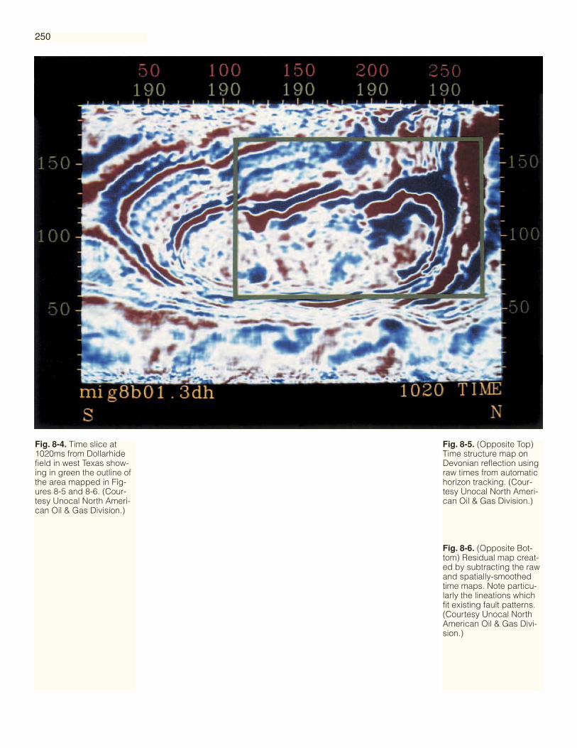
Fig. 8-4. Time slice at1020ms from Dollarhidefield in west Texas show-ing in green the outline ofthe area mapped in Fig-ures 8-5 and 8-6. (Cour-tesy Unocal North Ameri-can Oil & Gas Division.)

Fig. 8-5. (Opposite Top)Time structure map onDevonian reflection usingraw times from automatichorizon tracking. (Cour-tesy Unocal North Ameri-can Oil & Gas Division.)

Fig. 8-6. (Opposite Bot-tom) Residual map creat-ed by subtracting the rawand spatially-smoothedtime maps. Note particu-larly the lineations whichfit existing fault patterns.(Courtesy Unocal NorthAmerican Oil & Gas Divi-sion.)

250

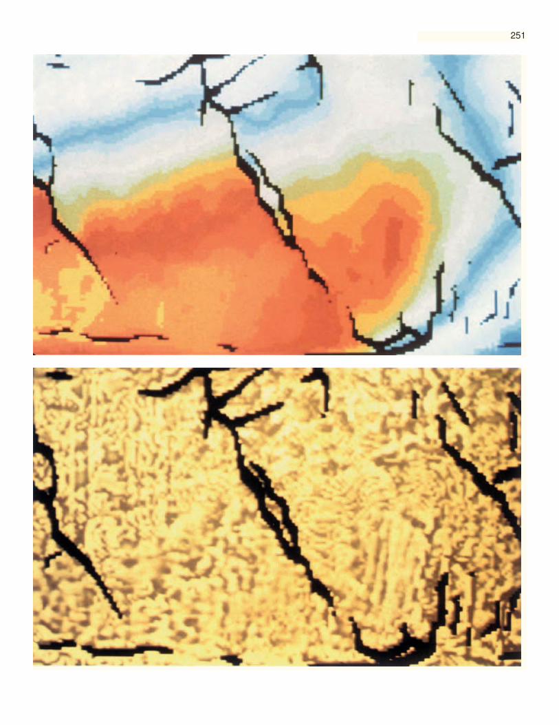
251

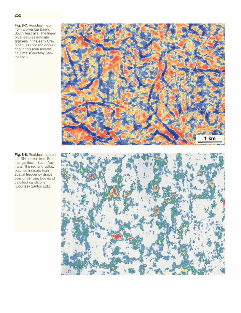
Fig. 8-7. Residual mapfrom Eromanga Basin,South Australia. The linearblue features indicategrabens in the early Cre-taceous C horizon occur-ring in this area around1100ms. (Courtesy San-tos Ltd.)

252

Fig. 8-8. Residual map onthe DN horizon from Ero-manga Basin, South Aus-tralia. The red and yellowpatches indicate highspatial frequency drapeover underlying bodies ofcalcified sandstone.(Courtesy Santos Ltd.)

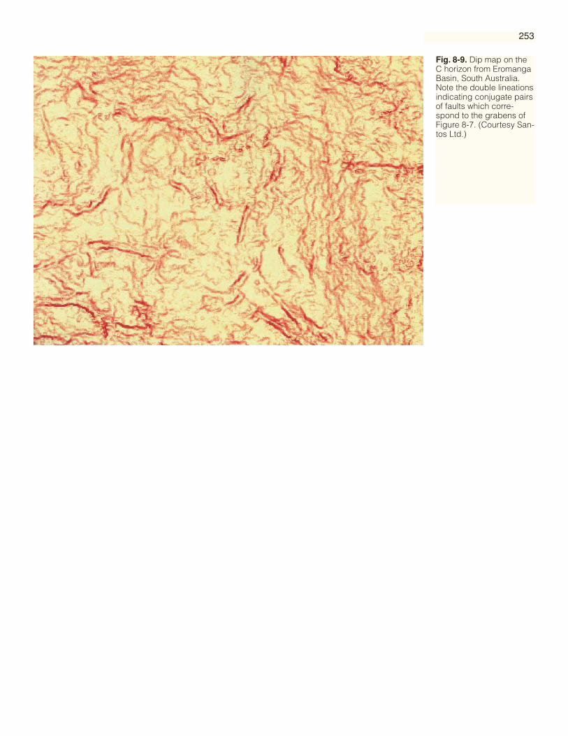
253

Fig. 8-9. Dip map on theC horizon from EromangaBasin, South Australia.Note the double lineationsindicating conjugate pairsof faults which corre-spond to the grabens ofFigure 8-7. (Courtesy San-tos Ltd.)

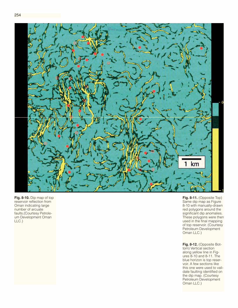
Fig. 8-10. Dip map of topreservoir reflection fromOman indicating largenumber of arcuatefaults.(Courtesy Petrole-um Development OmanLLC.)

Fig. 8-11. (Opposite Top)Same dip map as Figure8-10 with manually-drawnred polygons around thesignificant dip anomalies.These polygons were thenused in the final mappingof top reservoir. (CourtesyPetroleum DevelopmentOman LLC.)

Fig. 8-12. (Opposite Bot-tom) Vertical sectionalong yellow line in Fig-ures 8-10 and 8-11. Theblue horizon is top reser-voir. A few sections likethis one were used to vali-date faulting identified onthe dip map. (CourtesyPetroleum DevelopmentOman LLC.)

254

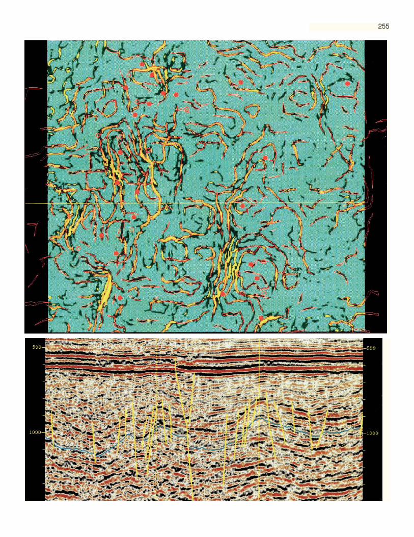
255

256

Time-derivedHorizon Attributes

automatic spatial tracking or snapping. These workstation capabilities help theinterpreter use all of the data and provide horizon time values at the crest of a reflec-tion with a precision of about a quarter of a millisecond. The horizon attributeextracted at the crestal time carries a similar precision. Proper use of machine preci-sion is a key part of seismic attribute analysis as the interpretation objective is nor-mally a rather detailed one. The quotation at the front of this book, “Believe every-thing to be geology until proved otherwise,” applies here. It is wise to put alldetailed information into the interpretation in the early stages and consider laterwhat is geology and what is noise. Attribute displays can be very helpful in thisimportant decision. Windowed attributes generally use the sample values every 2 or4 milliseconds.

Residual, or high spatial frequency residual map, is the arithmetic differencebetween a high-precision automatically-tracked time map and its spatially-smoothed equivalent. Figure 8-2 illustrates such a time map from Australia and Fig-ure 8-3 is the corresponding residual map (Denham and Nelson, 1986). There aretwo types of linear patterns on this residual. The NNW-SSE lineations are faults,mostly too subtle to be seen as contour disturbances on the time map. The exactly-parallel east-west lineations are in the data collection direction and are clearlycaused by data collection irregularities; this is a form of noise and is thereforeunwanted.

Figure 8-4 shows the area under study in the next example; Figure 8-5 is the auto-tracked high-precision time map; Figure 8-6 is the residual. The black features aregaps in the interpreted horizon which were recognized as faults in the mainstreamof the interpretation using vertical and horizontal sections. A linear pattern in theresidual parallel to the existing faults and towards the east end of the area is a ratherclear indication of another fault or similar geologic feature. In contrast, the north-south patterns towards the west end are highly regular and parallel and do not fitthe existing fault patterns; they must be identified as data collection lineations ornoise.

Figure 8-7 is a residual map from a land 3-D survey in South Australia; it is thetime difference between a snapped and a smoothed version of this early Cretaceoushorizon. The dark blue linear features are grabens. Blue means that the snappedhorizon is below the smoothed horizon thus establishing that these features arestructurally low.

Figure 8-8 is a similarly-produced residual map on another deeper horizon fromthe same survey. The red and yellow patches indicate high-spatial-frequency drapeover underlying bodies of calcified sandstone. The calcite varies rapidly both hori-zontally and vertically in this interval and therefore constitutes a serious problembecause of its effect on depth-conversion velocities for deeper horizons. This resid-ual map is helping to address the problem.

Dip, or dip magnitude, is another time-derived horizon attribute addressingissues of structural detail (Dalley et al., 1989). On the high-precision automatically-tracked time surface one time value is considered in relation to its immediate neigh-bors to form a local plane. The true dip of that local plane is the attribute dip; thedirection of that dip is the azimuth, or dip azimuth, which will be discussed later.

Figure 8-9 shows the dip map for the same horizon as used in Figure 8-7. Thedouble lineations indicate conjugate pairs of faults which correspond to the grabensof Figure 8-7 (Oldham and Gibbins, 1995).

Figure 8-10 shows the dip map for a top reservoir reflection from Oman. Manyarcuate features are evident. The color scheme was set so that all that was clearlynoise was suppressed into the gray-green; everything else was considered as apotential real fault. The red polygons in Figure 8-11 were drawn around the majorityof the dip anomalies and were then used directly in the mapping process. In draw-ing the red polygons and in deciding which dip anomalies were real, a few vertical

257

sections like Figure 8-12 were studied. The faults validated with a red polygon alongthe east-west yellow line in Figure 8-11 are shown in yellow in Figure 8-12.

Hesthammer (1998 and 1999) has studied subtle curvilinear features on dip andother attribute displays and concluded that many of them are noise. Coherent noise inthe seismic data intersects the horizon under study and causes steps that can look likefaults. Hesthammer concludes that the distinction between real, subtle faults andnoise can be difficult, and this problem most likely exists in Figures 8-9 and 8-10. Thebasis for distinguishing must be geological reasonableness.

Figure 8-13 shows the dip map of a horizon which was autotracked with little verti-cal and horizontal section control. Although the tracking was successful over much ofthe area, the tracker jumped onto the wrong event in several places. These trackingbusts show as very straight high-dip pseudo-faults primarily in green and blue. Thisdemonstrates that time-derived attribute displays such as dip can be used to qualitycontrol the performance of an autotracker as well as to establish further structuraldetail.

Azimuth, or dip azimuth, is used in a similar way to dip. Figure 8-14 shows anexample of an azimuth map from Lake Maracaibo, Venezuela. The data is clearlynoisy but nonetheless several meaningful patterns can be seen. The red arrows indi-cate anomalies which conform with existing fault patterns and are thus probableadditional faulting. Two of the indicated faults are magenta and blue and thus dip tothe northeast; the third is red and yellow and thus dips to the southwest.

Figures 8-15 and 8-16 show a pair of dip and azimuth displays from Nigeria. Bothshow many faults which are generally the same. However, red arrows indicate twofaults, each of which is visible on only one of the displays. For a subtle fault the dip ofthe fault can accidentally concur with the dip of the surrounding horizon surface;likewise separately for the azimuth. It is thus wise to look at more than one type ofattribute display in order to reduce the chance of missing something significant.

A dip-azimuth combination map (Figure 8-17) combines the separate dip andazimuth attributes onto the one display and is thus an alternative approach to thefault visibility problem discussed above. In Figure 8-17 he dip is coded to color densi-ty and the azimuth is coded to hue according to the circular legend. Many faults asso-ciated with salt movement are visible.

Curvature and roughness are derivatives of dip and azimuth and thus serve as sec-ond derivatives of structure. Figure 8-18 illustrates these attributes and comparesthem with azimuth for the same horizon surface.

Edge, or edge detection, is a spatial operator usually occupying 9 points whichoperates like a spatial smoothing filter but has the opposite effect; spatial differencesor edges are accentuated regardless of orientation. Figure 8-19 is an edge map on thetop Tosca reflection in the Neuquen Basin of Argentina. In the west there is a swarmof north-south faults and several 7-km-long arcuate faults. These arcuate faults lookimpressive on the edge map but have a barely-visible displacement on vertical sec-tions. Similar arcuate patterns on the edge maps from deeper horizons indicate thatthese faults are in fact conical in shape pointing downwards with their apexes on anigneous intrusion.

Figure 8-20 is an edge map from southern Alberta in Canada here being used todelineate a reef.

Illumination, lighting, shaded relief or sun shading is a display technique alreadywell known from topographic and other kinds of mapping. Portions of the auto-tracked time surface pointing towards the source are highlighted, those pointingaway from the source are in shadow. Figure 8-21 has an illumination direction fromthe northwest. The fault running north-south down the west side is highlighted. Justeast of this is a sequence of en echelon faults in shadow. Just southeast of center is aclearly visible graben.

Figures 8-22 and 8-23 show the same time surface with different illumination direc-tions as shown by the red arrows. Faults highlighted on one are in shadow on the otherand vice versa. This is marine data collected in the northwest-southeast direction. With

Text continues on page 274

258

Fig. 8-13. Dip map usedas quality control of auto-matic tracker perfor-mance. The very straight,high-dip pseudo-faultsare tracking busts. (Cour-tesy Nederlandse Aar-dolie Maatschappij B.V.)

259

Fig. 8-14. Azimuth mapfrom Lake Maracaibo,Venezuela. Red arrowsindicate anomalies whichconform well to existingfault patterns and are thusprobable additional fault-ing. (Courtesy MaravenS.A.)

260

261

Fig. 8-17. Dip-azimuthcombination map from off-shore The Netherlands.Azimuth is coded to hueaccording to legend; dipis coded to color density.The horizon is just abovea salt dome located in theSW corner. (CourtesyNederlandse AardolieMaatschappij B.V.)

Fig. 8-15. (Opposite Top) Dipmap from Nun River field, Nige-ria, showing many faults (fromBouvier et al, 1989). Arrow indi-cates one fault visible on dipmap but not on azimuth map inFigure 8-16. (Courtesy Konin-klijke / Shell.)

Fig. 8-16. (Opposite Bottom)Azimuth map from Nun Riverfield, Nigeria, showing generallythe same faults as in Figure 8-15 (from Bouvier et al, 1989).Arrow indicates one fault visiblein azimuth but not in dip. (Cour-tesy Koninklijke / Shell.)

262

Fig. 8-18. Maps of azimuth(top), curvature (middle)and roughness (bottom) forsame horizon. Curvatureand roughness are thederivatives of dip andazimuth and help to high-light flexures. (CourtesyFlagship GeosciencesL.L.C.)

263

Fig. 8-19. Edge map fromNeuquen Basin, Argenti-na. Arcuate faults about 7km long have barely-visi-ble displacements on ver-tical sections. (CourtesyPetrolera Argentina SanJorge S.A.)

Fig. 8-20. Edge map fromsouthern Alberta, Cana-da, outlining reef. (Cour-tesy Landmark GraphicsCorporation.)

Fig. 8-21. Illumination dis-play or shaded relief mapon Base Zechstein refec-tion from Annerveen gasfield, The Netherlands(from Hoetz and Watters,1992). The direction ofillumination is from thenorthwest. Note thegraben just SE of center.(Courtesy NederlandseAardolie MaatschappijB.V.)

264

265

Fig. 8-22. Illumination dis-play of horizon fromGoodwyn field, NorthwestShelf, Australia. The direc-tion of illumination is fromthe northwest. (CourtesyWoodside Offshore Petro-leum Pty. Ltd.)

Fig. 8-23. Illumination dis-play of horizon fromGoodwyn field, NorthwestShelf, Australia. The direc-tion of illumination is fromthe northeast for compari-son with Figure 8-22. Notehow the data collectionlineations are now visible.(Courtesy Woodside Off-shore Petroleum Pty. Ltd.)

266

Fig

.8-2

4.C

oher

ence

tim

e sl

ice

at15

25m

s fro

m G

ulf o

f Mex

ico.

Are

aco

vers

60

blo

cks.

Not

e, b

y co

m-

par

ison

with

Fig

ure

8-25

, how

faul

ts a

re e

qua

lly v

isib

le w

hen

par

alle

l to

or p

erp

end

icul

ar to

stru

ctur

al s

trik

e. (

Cou

rtes

y A

moc

oC

orp

orat

ion.

)

267

Fig

.8-2

5.Ti

me

slic

e at

152

5ms

from

Gul

f of M

exic

o fo

r co

mp

ari-

son

with

Fig

ure

8-24

. (C

ourt

esy

Am

oco

Cor

por

atio

n.)

Fig. 8-26. Coherence timeslice at 1640ms fromNorth Sea (from Bahorichet al, 1995). (CourtesyAmoco Corporation.)

Fig. 8-27. Time slice at1640ms from North Seafor comparison with Fig-ure 8-26 (from Bahorich etal, 1995). (CourtesyAmoco Corporation.)

268

269

Fig. 8-28. Continuity timeslice at about 1500msfrom Gulf of Mexico show-ing many radial faults.(Courtesy CAEX Servicesand Landmark AdvanceProducts Group.)

Fig. 8-29. Time slice atabout 1500ms from Gulfof Mexico for comparisonwith Figure 8-28. (Cour-tesy CAEX Services andLandmark Advance Prod-ucts Group.)

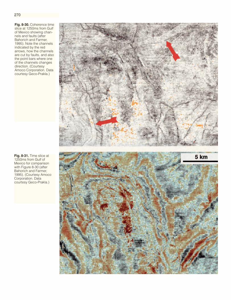
Fig. 8-30. Coherence timeslice at 1250ms from Gulfof Mexico showing chan-nels and faults (afterBahorich and Farmer,1995). Note the channelsindicated by the redarrows, how the channelsare cut by faults, and alsothe point bars where oneof the channels changesdirection. (CourtesyAmoco Corporation. Datacourtesy Geco-Prakla.)

270

Fig. 8-31. Time slice at1250ms from Gulf ofMexico for comparisonwith Figure 8-30 (afterBahorich and Farmer,1995). (Courtesy AmocoCorporation. Datacourtesy Geco-Prakla.)

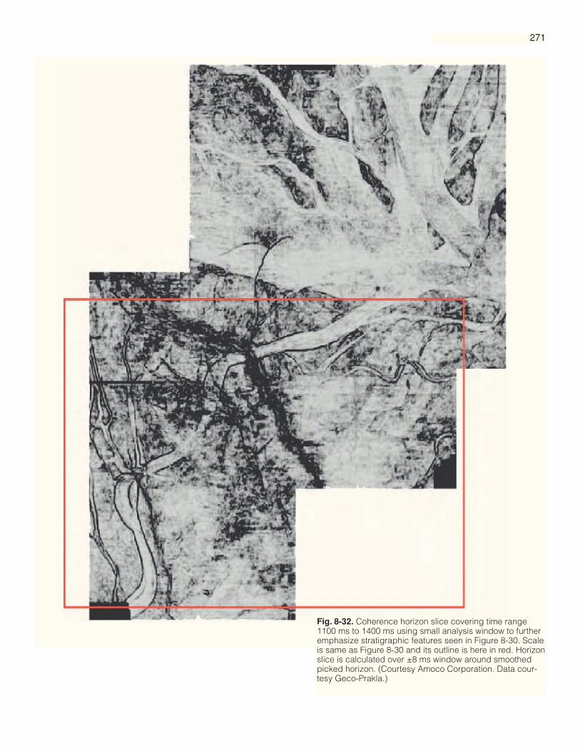
271

Fig. 8-32. Coherence horizon slice covering time range1100 ms to 1400 ms using small analysis window to furtheremphasize stratigraphic features seen in Figure 8-30. Scaleis same as Figure 8-30 and its outline is here in red. Horizonslice is calculated over ±8 ms window around smoothedpicked horizon. (Courtesy Amoco Corporation. Data cour-tesy Geco-Prakla.)

Fig. 8-33. Coherence timeslice at 2800 ms from Val-hall area of the North Sea.The polygonal fault pat-tern results from com-pactional dewatering ofoverpressured shales.(Courtesy Amoco Corpo-ration.)

272

273

Fig. 8-35. Coherence timeslice from Canada show-ing dendritic channel pat-terns. (Courtesy Coher-ence TechnologyCompany.)

Fig. 8-34. Coherence timeslice at 2600 ms from theNorth Sea showing pat-terns of sub-salt Carbonif-erous faulting. (CourtesyCoherence TechnologyCompany.)

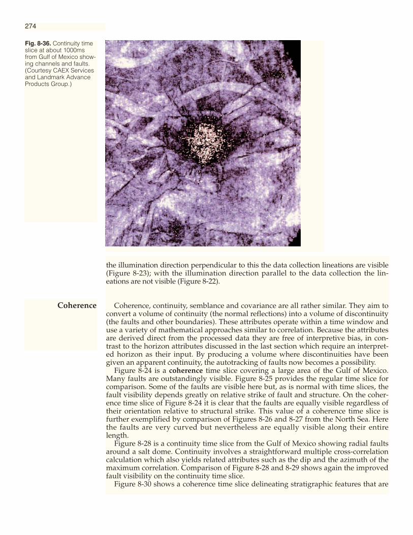
Coherence

274

Fig. 8-36. Continuity timeslice at about 1000msfrom Gulf of Mexico show-ing channels and faults.(Courtesy CAEX Servicesand Landmark AdvanceProducts Group.)

the illumination direction perpendicular to this the data collection lineations are visible(Figure 8-23); with the illumination direction parallel to the data collection the lin-eations are not visible (Figure 8-22).

Coherence, continuity, semblance and covariance are all rather similar. They aim toconvert a volume of continuity (the normal reflections) into a volume of discontinuity(the faults and other boundaries). These attributes operate within a time window anduse a variety of mathematical approaches similar to correlation. Because the attributesare derived direct from the processed data they are free of interpretive bias, in con-trast to the horizon attributes discussed in the last section which require an interpret-ed horizon as their input. By producing a volume where discontinuities have beengiven an apparent continuity, the autotracking of faults now becomes a possibility.

Figure 8-24 is a coherence time slice covering a large area of the Gulf of Mexico.Many faults are outstandingly visible. Figure 8-25 provides the regular time slice forcomparison. Some of the faults are visible here but, as is normal with time slices, thefault visibility depends greatly on relative strike of fault and structure. On the coher-ence time slice of Figure 8-24 it is clear that the faults are equally visible regardless oftheir orientation relative to structural strike. This value of a coherence time slice isfurther exemplified by comparison of Figures 8-26 and 8-27 from the North Sea. Herethe faults are very curved but nevertheless are equally visible along their entirelength.

Figure 8-28 is a continuity time slice from the Gulf of Mexico showing radial faultsaround a salt dome. Continuity involves a straightforward multiple cross-correlationcalculation which also yields related attributes such as the dip and the azimuth of themaximum correlation. Comparison of Figure 8-28 and 8-29 shows again the improvedfault visibility on the continuity time slice.

Figure 8-30 shows a coherence time slice delineating stratigraphic features that are

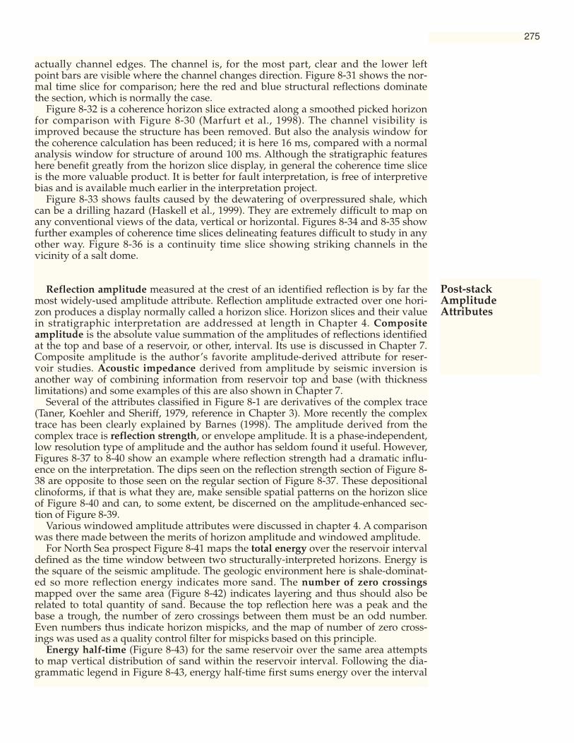
275

Post-stackAmplitudeAttributes

actually channel edges. The channel is, for the most part, clear and the lower leftpoint bars are visible where the channel changes direction. Figure 8-31 shows the nor-mal time slice for comparison; here the red and blue structural reflections dominatethe section, which is normally the case.

Figure 8-32 is a coherence horizon slice extracted along a smoothed picked horizonfor comparison with Figure 8-30 (Marfurt et al., 1998). The channel visibility isimproved because the structure has been removed. But also the analysis window forthe coherence calculation has been reduced; it is here 16 ms, compared with a normalanalysis window for structure of around 100 ms. Although the stratigraphic featureshere benefit greatly from the horizon slice display, in general the coherence time sliceis the more valuable product. It is better for fault interpretation, is free of interpretivebias and is available much earlier in the interpretation project.

Figure 8-33 shows faults caused by the dewatering of overpressured shale, whichcan be a drilling hazard (Haskell et al., 1999). They are extremely difficult to map onany conventional views of the data, vertical or horizontal. Figures 8-34 and 8-35 showfurther examples of coherence time slices delineating features difficult to study in anyother way. Figure 8-36 is a continuity time slice showing striking channels in thevicinity of a salt dome.

Reflection amplitude measured at the crest of an identified reflection is by far themost widely-used amplitude attribute. Reflection amplitude extracted over one hori-zon produces a display normally called a horizon slice. Horizon slices and their valuein stratigraphic interpretation are addressed at length in Chapter 4. Compositeamplitude is the absolute value summation of the amplitudes of reflections identifiedat the top and base of a reservoir, or other, interval. Its use is discussed in Chapter 7.Composite amplitude is the author’s favorite amplitude-derived attribute for reser-voir studies. Acoustic impedance derived from amplitude by seismic inversion isanother way of combining information from reservoir top and base (with thicknesslimitations) and some examples of this are also shown in Chapter 7.

Several of the attributes classified in Figure 8-1 are derivatives of the complex trace(Taner, Koehler and Sheriff, 1979, reference in Chapter 3). More recently the complextrace has been clearly explained by Barnes (1998). The amplitude derived from thecomplex trace is reflection strength, or envelope amplitude. It is a phase-independent,low resolution type of amplitude and the author has seldom found it useful. However,Figures 8-37 to 8-40 show an example where reflection strength had a dramatic influ-ence on the interpretation. The dips seen on the reflection strength section of Figure 8-38 are opposite to those seen on the regular section of Figure 8-37. These depositionalclinoforms, if that is what they are, make sensible spatial patterns on the horizon sliceof Figure 8-40 and can, to some extent, be discerned on the amplitude-enhanced sec-tion of Figure 8-39.

Various windowed amplitude attributes were discussed in chapter 4. A comparisonwas there made between the merits of horizon amplitude and windowed amplitude.

For North Sea prospect Figure 8-41 maps the total energy over the reservoir intervaldefined as the time window between two structurally-interpreted horizons. Energy isthe square of the seismic amplitude. The geologic environment here is shale-dominat-ed so more reflection energy indicates more sand. The number of zero crossingsmapped over the same area (Figure 8-42) indicates layering and thus should also berelated to total quantity of sand. Because the top reflection here was a peak and thebase a trough, the number of zero crossings between them must be an odd number.Even numbers thus indicate horizon mispicks, and the map of number of zero cross-ings was used as a quality control filter for mispicks based on this principle.

Energy half-time (Figure 8-43) for the same reservoir over the same area attemptsto map vertical distribution of sand within the reservoir interval. Following the dia-grammatic legend in Figure 8-43, energy half-time first sums energy over the interval

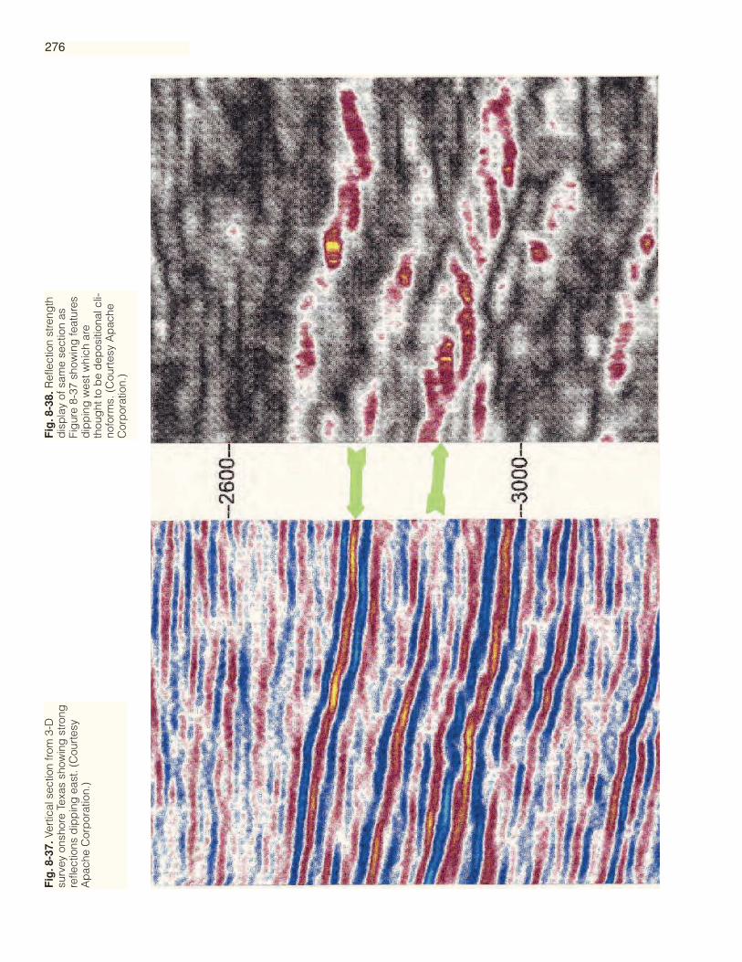
Fig

.8-3

7.Ve

rtic

al s

ectio

n fro

m 3

-Dsu

rvey

ons

hore

Tex

as s

how

ing

stro

ngre

flect

ions

dip

pin

g e

ast.

(Cou

rtes

yA

pac

he C

orp

orat

ion.

)

Fig

.8-3

8.R

efle

ctio

n st

reng

thd

isp

lay

of s

ame

sect

ion

asFi

gur

e 8-

37 s

how

ing

feat

ures

dip

pin

g w

est w

hich

are

thou

ght

to b

e d

epos

ition

al c

li-no

form

s. (

Cou

rtes

y A

pac

heC

orp

orat

ion.

)

276

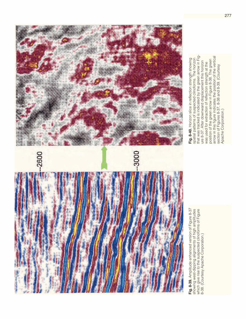
Fig

.8-3

9.A

mp

litud

e en

hanc

ed v

ersi

on o

f Fig

ure

8-37

show

ing

wes

t-d

ipp

ing

alig

nmen

ts o

f hig

h am

plit

udes

whi

ch g

ive

rise

to th

e su

spec

ted

clin

ofor

ms

of F

igur

e8-

38. (

Cou

rtes

y A

pac

he C

orp

orat

ion.

)

Fig

.8-4

0.H

oriz

on s

lice

in re

flect

ion

stre

ngth

sho

win

gsp

atia

l pat

tern

s of

sus

pec

ted

clin

ofor

ms.

The

hor

izon

that

was

trac

ked

is in

dic

ated

by

the

gre

en a

rrow

in F

ig-

ure

8-37

. Afte

r d

ownw

ard

dis

pla

cem

ent t

his

horiz

onw

as u

sed

for

extr

actio

n of

refle

ctio

n st

reng

th a

t the

pos

ition

of t

he g

reen

arr

ow in

Fig

ure

8-38

. The

gre

enar

row

in th

is fi

gur

e in

dic

ates

the

pos

ition

of t

he v

ertic

alse

ctio

n of

Fig

ures

8-3

7, 8

-38

and

8-3

9. (

Cou

rtes

yA

pac

he C

orp

orat

ion.

)

277

278

279

Fig. 8-43. Energy half-time map over reservoirinterval from North Sea indicating vertical dis-tribution of sands within the reservoir. (Cour-tesy BP Exploration and P. Mulholland.)

Fig. 8-41. (Opposite Top) Seismic energy map over reservoir interval fromNorth Sea. High energy indicates sand in a shale-dominated environment.(Courtesy BP Exploration and P. Mulholland.)

Fig. 8-42. (Opposite Bottom) Number of zero crossings over reservoirinterval from North Sea. This map indicates layering and also serves asquality control filter for horizon mispicks. (Courtesy BP Exploration and P.Mulholland.)

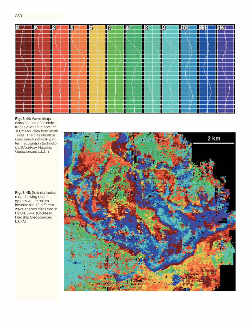
Fig. 8-44. Wave shapeclassification of seismictraces over an interval of100ms for data from southTexas. The classificationuses neural network pat-tern recognition technolo-gy. (Courtesy FlagshipGeosciences L.L.C.)

Fig. 8-45. Seismic faciesmap showing channelsystem where colorsindicate the 12 differentwave shapes classified inFigure 8-44. (CourtesyFlagship GeosciencesL.L.C.)

280

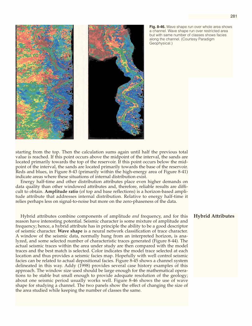
281

starting from the top. Then the calculation sums again until half the previous totalvalue is reached. If this point occurs above the midpoint of the interval, the sands arelocated primarily towards the top of the reservoir. If this point occurs below the mid-point of the interval, the sands are located primarily towards the base of the reservoir.Reds and blues, in Figure 8-43 (primarily within the high-energy area of Figure 8-41)indicate areas where these situations of internal distribution exist.

Energy half-time and other distribution attributes place even higher demands ondata quality than other windowed attributes and, therefore, reliable results are diffi-cult to obtain. Amplitude ratio (of top and base reflections) is a horizon-based ampli-tude attribute that addresses internal distribution. Relative to energy half-time itrelies perhaps less on signal-to-noise but more on the zero-phaseness of the data.

Hybrid attributes combine components of amplitude and frequency, and for thisreason have interesting potential. Seismic character is some mixture of amplitude andfrequency; hence, a hybrid attribute has in principle the ability to be a good descriptorof seismic character. Wave shape is a neural network classification of trace character.A window of the seismic data, normally hung from an interpreted horizon, is ana-lyzed, and some selected number of characteristic traces generated (Figure 8-44). Theactual seismic traces within the area under study are then compared with the modeltraces and the best match is selected. Color indicates the model trace selected at eachlocation and thus provides a seismic facies map. Hopefully with well control seismicfacies can be related to actual depositional facies. Figure 8-45 shows a channel systemdelineated in this way. Addy (1998) provides several case history examples of thisapproach. The window size used should be large enough for the mathematical opera-tions to be stable but small enough to provide adequate resolution of the geology;about one seismic period usually works well. Figure 8-46 shows the use of waveshape for studying a channel. The two panels show the effect of changing the size ofthe area studied while keeping the number of classes the same.

Hybrid Attributes

Fig. 8-46. Wave shape run over whole area showsa channel. Wave shape run over restricted areabut with same number of classes shows faciesalong the channel. (Courtesy ParadigmGeophysical.)

282

Fig. 8-47. Loop area wasused to generate thisaverage porosity map fora carbonate member ofthe Zechstein formation inHolland. (Courtesy Neder-landse AardolieMaatschappij B.V.)

Fig. 8-48. Loop area andarc length explanation.

287

Fig. 8-54. Vertical sectionshowing 250-ms windowcovering the productivesands. This window wasused for the attribute cal-culations for Figures 8-52and 8-53. (Courtesy YPFS.A.)

it must be secondary to the frequency characteristics of the propagating wavelet. Inthe three following examples it appears that geologic frequency is being expressed ina seismic frequency measurement.

Figures 8-52 and 8-53 show average instantaneous frequency and number of zerocrossings for the oil-bearing interval shown as a 250-ms window in Figure 8-54. Thefield in southern Argentina has many wells producing from many thin sands of limit-ed lateral extent. More layering should mean more sand. The wells were drilled on aregular pattern basis from the initial discovery, and are in fact clustered at the loca-tions marked by red arrows. High frequency for both attributes thus correlates withbetter production from more sands.

A similar story is reported from south Texas by Horkowitz and Davis (1996). Figure8-55 shows an RMS instantaneous frequency map from an area with many wells. Thewells with more sands lie in the areas of high instantaneous frequency.

First, second and third dominant frequencies involve completely different trans-form mathematics and notionally force-fit the spectrum to yield three maxima. Firstdominant frequency should primarily express the properties of the wavelet. Seconddominant frequency should primarily express the geologic frequency and thus be themost useful. For the window of data shown in the small insert of Figure 8-51, seconddominant frequency, first dominant frequency and composite amplitude were cross-plotted to yield Figure 8-56. The white points, well separated in second dominant fre-quency, are plotted in their proper geographic position in Figure 8-57. The color indi-cates amplitude and the existence of hydrocarbon. The white dots are believed toindicate additional layering and thus additional sand. In fact a well was drilled intoone of the areas of white dots and found some previously bypassed reserves.

288

Fig. 8-55. RMS instanta-neous frequency mapover 40ms interval fromsouth Texas. The wells inthe high instantaneousfrequency areas containmore layers of sand.(Courtesy Sanchez-O’Brien Oil and Gas Cor-poration and K. O.Horkowitz.)

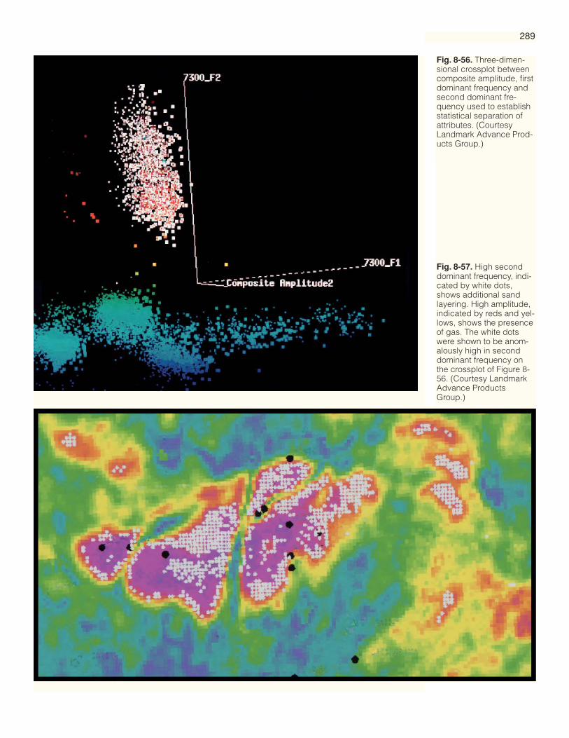
289

Fig. 8-56. Three-dimen-sional crossplot betweencomposite amplitude, firstdominant frequency andsecond dominant fre-quency used to establishstatistical separation ofattributes. (CourtesyLandmark Advance Prod-ucts Group.)

Fig. 8-57. High seconddominant frequency, indi-cated by white dots,shows additional sandlayering. High amplitude,indicated by reds and yel-lows, shows the presenceof gas. The white dotswere shown to be anom-alously high in seconddominant frequency onthe crossplot of Figure 8-56. (Courtesy LandmarkAdvance ProductsGroup.)

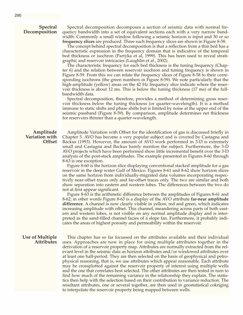
Spectral decomposition decomposes a section of seismic data with normal fre-quency bandwidth into a set of equivalent sections each with a very narrow band-width. Commonly a small window following a seismic horizon is input and 30 or sofrequency slices are produced. Three such frequency slices are shown in Figure 8-58.

The concept behind spectral decomposition is that a reflection from a thin bed has acharacteristic expression in the frequency domain that is indicative of the temporalbed thickness or isochron (Partyka et al, 1999). This has been used to reveal strati-graphic and reservoir intricacies (Laughlin et al., 2002).

The characteristic frequency for each bed thickness is the tuning frequency (Chap-ter 6) and the relation between reservoir isochron and tuning frequency is shown inFigure 8-59. From this we can relate the frequency slices of Figure 8-58 to their corre-sponding isochrons (the green numbers in Figure 8-59). We note particularly that thehigh-amplitude (yellow) areas on the 42 Hz frequency slice indicate where the reser-voir thickness is about 12 ms. This is below the tuning thickness (17 ms) of the full-bandwidth data.

Spectral decomposition, therefore, provides a method of determining gross reser-voir thickness below the tuning thickness (or quarter-wavelength). It is a methodimmune to static shifts and phase shifts but is limited by noise at the upper end of theseismic passband (Figure 8-59). By comparison, amplitude determines net thicknessfor reservoirs thinner than a quarter-wavelength.

Amplitude Variation with Offset for the identification of gas is discussed briefly inChapter 5. AVO has become a very popular subject and is covered by Castagna andBackus (1993). However, the amount of AVO work performed in 3-D is extremelysmall and Castagna and Backus barely mention the subject. Furthermore, the 3-DAVO projects which have been performed show little incremental benefit over the 3-Danalysis of the post-stack amplitudes. The example presented in Figures 8-60 through8-63 is one exception.

Figure 8-60 is the horizon slice displaying conventional stacked amplitude for a gasreservoir in the deep water Gulf of Mexico. Figures 8-61 and 8-62 show horizon sliceson the same horizon from individually-migrated data volumes incorporating respec-tively near-offset traces only and far-offset traces only. The two are similar and bothshow separation into eastern and western lobes. The differences between the two donot at first appear significant.

Figure 8-63 is the arithmetic difference between the amplitudes of Figures 8-61 and8-62; in other words Figure 8-63 is a display of the AVO attribute far-near amplitudedifference. A channel is now clearly visible in yellow, red and green, which indicatesincreasing amplitude with offset. This channel, meandering across parts of both east-ern and western lobes, is not visible on any normal amplitude display and is inter-preted as the sand-filled channel facies of a slope fan. Furthermore, it probably indi-cates the areas of highest porosity and permeability within the reservoir.

This chapter has so far focussed on the attributes available and their individualuses. Approaches are now in place for using multiple attributes together in thederivation of a reservoir property map. Attributes are normally extracted from the rel-evant level in the seismic data as horizon attributes and/or windowed attributes overat least one half-period. They are then selected on the basis of geophysical and petro-physical reasoning, that is, we use attributes which appear reasonable. Each attributemay be crossplotted against the reservoir property of interest using multiple wellsand the one that correlates best selected. The other attributes are then tested in turn tofind how much of the remaining variance in the relationship they explain. The statis-tics then help with the selection based on their contribution to variance reduction. Theresultant attributes, one or several together, are then used in geostatistical cokrigingto interpolate the reservoir property being mapped between wells.

290

SpectralDecomposition

AmplitudeVariation with

Offset

Use of MultipleAttributes

291

Fig. 8-58. Frequencyslices at 22 Hz, 32 Hz and42 Hz obtained by Spec-tral Decomposition. Thecolors indicate amplitudein a narrow band aroundthe frequency indicated.(Courtesy LandmarkGraphics.)

Fig. 8-59. The principle ofSpectral Decomposition.Each reservoir isochronhas a corresponding tun-ing frequency. (CourtesyLandmark Graphics.)

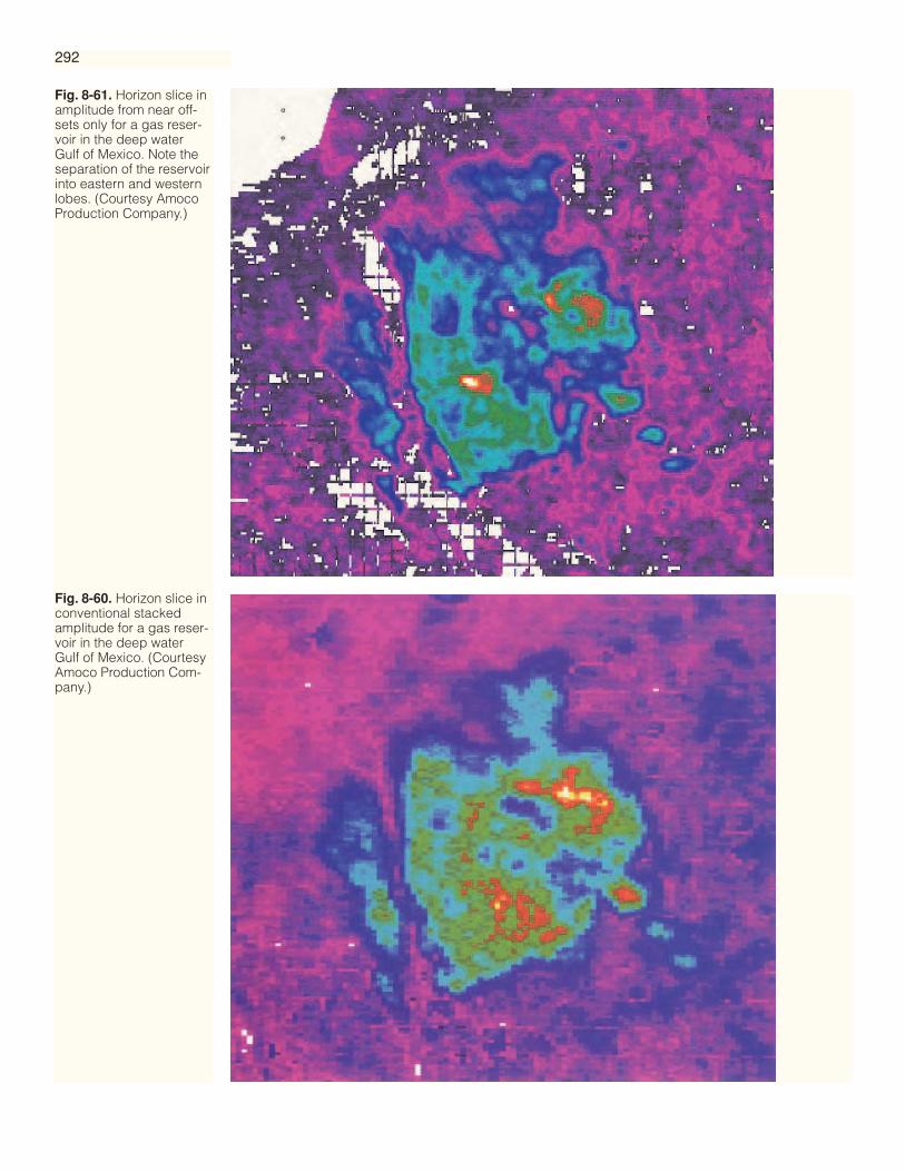
292

Fig. 8-60. Horizon slice inconventional stackedamplitude for a gas reser-voir in the deep waterGulf of Mexico. (CourtesyAmoco Production Com-pany.)

Fig. 8-61. Horizon slice inamplitude from near off-sets only for a gas reser-voir in the deep waterGulf of Mexico. Note theseparation of the reservoirinto eastern and westernlobes. (Courtesy AmocoProduction Company.)

293

Fig. 8-62. Horizon slice inamplitude from far offsetsonly for comparison withFigure 8-61. (CourtesyAmoco ProductionCompany.)

Fig. 8-63. 3-D AVO —horizon slice in far-nearamplitude difference, thatis, the subtraction ofFigure 8-61 amplitudesfrom Figure 8-62amplitudes. Reds, yellowsand greens indicateamplitude increasing withoffset. The pattern inthese colors indicates achannel not visible innormal amplitude andprobably containing thehighest porosities andpermeabilities in the fan.(Courtesy AmocoProduction Company.)

There are many dangers in statistics and much has recently been written aboutthese dangers as applied to reservoir characterization. Hirsche et al. (1997 and 1998)has been particularly vocal with remarks including: Neglecting geology and geophysicsreduces geostatistics to a purely statistical process that may give false confidence in spuriousresults. Schuelke and Quirein (1998) offer a similar caution: The use of statistical methodswithout the foundation of a physical basis for the correlation between the seismic attribute(s)and the rock property … is very risky. Hart (2002) makes the same point: There must be aknown or suspected link between the attribute and the log-based physical properties to beimaged. Hart and Balch (1999) remind us that the probability of obtaining a statisticallysignificant but spurious correlation between an attribute and a log-derived property is propor-tional to the number of attributes tested and inversely proportional to the number of wellsused in the calibration. Kalkomey (1997) discusses this further and calculates alarming-ly high probabilities.

In summary, for a geostatistical reservoir study we would like a large number ofwells but we should not use a large number of attributes. Thus about three, or up to amaximum of five, attributes should be selected primarily on the basis of geophysicaland petrophysical reasoning. Little reliance should be placed on correlation coeffi-cients. The selected attributes are then submitted to the multiple regression analysisand cokriging.

294

295

Visualization of Horizon Attributes

Contributed by Geoffrey A. DornARCO Exploration and Production Technology (now University of Colorado at Boulder)

Visualization is the graphical presentation of data in an intuitive fashion thatexposes the information in the data and provides new insight. Common examples ofvisualization include pie charts, bar graphs or xy plots, seismic sections, time slices,and contour maps. A structure contour map is an attempt to represent a three-dimen-sional surface in a two-dimensional display. Horizon attributes are typically visual-ized as two-dimensional map displays where the variation in the attribute value iscalibrated to a particular color range. Three-dimensional visualization attempts toconvey significantly more information through the representation of multi-parametricdata in three dimensional surfaces and volumes.

The most common form used to represent a three-dimensional surface has formany years been the contour map. Each color on this type of map represents a rangeof times. The appearance of a continuous gradation can be achievable by using a larg-er number of individual color bins. By looking at a contour map, and understandingfrom the legend the relationship between color and structural highs and lows, it ispossible to form a mental image of the three-dimensional surface.

This representation of the 3-D surface is limited because it requires mental integra-tion of complex variations of data along the three dimensional structure. For example,it becomes more difficult to form a correct mental picture when the structural infor-mation must be combined with reflection amplitude along the interpreted horizonshown in Figure 8-64. The problem becomes even more complex in a practical situa-tion when there is a need to integrate the information from structure, several horizonattributes, some well locations, and possibly culture.

These difficulties can be managed by using 3-D visualization to represent the data.In Figure 8-65, for example, the interpreted horizon is now shown a three-dimension-al surface, with the reflection amplitude shown in color. It now becomes a simply amatter of observation to identify the relationship, if any, between the structure andthe horizon attribute.

There are a number of cues that the mind uses to perceive and understand a three-dimensional object. These include:

- Projection- Lighting and shading- Depth of field- Depth cueing- Obscuration- Transparency- Stereopsis- Parallax- Motion

Projection refers to a method of graphically depicting three-dimensional objectsand spatial relationships on a two-dimensional plane (Foley, et al., 1990). A perspec-tive projection is one in which parallel lines and planes converge to infinitely distantvanishing points. In a parallel projection, parallel lines and planes are made to betruly parallel in the display. This may result in an optical distortion in the perceptionof three dimensions, but can provide a display (e.g. an isometric orthographic parallel

Nature ofVisualization

Perception ofThreeDimensions

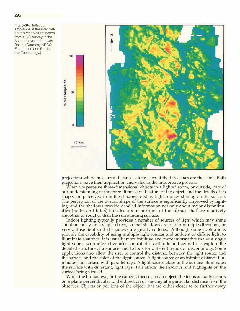
projection) where measured distances along each of the three axes are the same. Bothprojections have their application and value in the interpretive process.

When we perceive three-dimensional objects in a lighted room, or outside, part ofour understanding of the three-dimensional nature of the object, and the details of itsshape, are perceived from the shadows cast by light sources shining on the surface.The perception of the overall shape of the surface is significantly improved by light-ing, and the shadows provide detailed information not only about major discontinu-ities (faults and folds) but also about portions of the surface that are relativelysmoother or rougher than the surrounding surface.

Indoor lighting typically provides a number of sources of light which may shinesimultaneously on a single object, so that shadows are cast in multiple directions, orvery diffuse light so that shadows are greatly softened. Although some applicationsprovide the capability of using multiple light sources and ambient or diffuse light toilluminate a surface, it is usually more intuitive and more informative to use a singlelight source with interactive user control of its altitude and azimuth to explore thedetailed structure of a surface, and to look for different trends of discontinuity. Someapplications also allow the user to control the distance between the light source andthe surface and the color of the light source. A light source at an infinite distance illu-minates the surface with parallel rays. A light source close to the surface illuminatesthe surface with diverging light rays. This affects the shadows and highlights on thesurface being viewed.

When the human eye, or the camera, focuses on an object, the focus actually occurson a plane perpendicular to the direction of viewing at a particular distance from theobserver. Objects or portions of the object that are either closer to or further away

296

Fig. 8-64. Reflectionamplitude at the interpret-ed top reservoir reflectionfrom a 3-D survey in theSouthern North Sea GasBasin. (Courtesy ARCOExploration and Produc-tion Technology.)

from the observer are out of focus. This phenomenon is called depth of field (Foley, etal., 1990). Although this is an additional cue to the relative distance to parts of anobject, it is typically not used in technical applications that render data in threedimensions. If this technique were used, it would require re-rendering the image toclearly view different depths on the surface or in the volume which would be bothtime consuming and awkward. Typically the entire three-dimensional surface or vol-ume is rendered in focus allowing the user to examine all depths in the image simul-taneously with essentially the same clarity.

Depth cueing refers to a phenomenon where the more distant objects are renderedwith a lower intensity than nearer objects. This can be viewed as a type of “atmos-pheric” attenuation. This can be important in lending realism to a computer generat-ed image of a scene or structure. It is usually not desirable when rendering complexthree-dimensional data for analysis.

Obscuration is a process where the nearer portions of a complex three-dimensionalsurface may obstruct or block the view of portions of the surface that are further awayfrom the viewer. Other terms for this are visible line/surface determination and hid-den line/surface removal. This is done as a matter of course in the three-dimensionalrendering of opaque surfaces and solids. By allowing the interpreter control over thetransparency of the rendered surfaces, it is possible to see through one horizon to thedata that would be hidden behind it if it were opaque. The partial transparency of thenearer surface gives the mind very clear information about the relative position of thesurfaces.

Stereopsis refers to the ability to view an object simultaneously from two slightlydifferent directions and composite the three-dimensional image. Most people arenaturally able, and accustomed, to see three-dimensional objects stereoscopically.Stereoscopic displays have seen relatively limited use to date in three-dimensionalinterpretation, but their use will increase over time. The increase in the amount of

297

Fig. 8-65. Interpreted timestructure of the top reser-voir reflection with reflec-tion amplitude in color,shown as a three-dimen-sional surface in perspec-tive view. (CourtesyARCO Exploration andProduction Technology.)

298

Fig. 8-66. Lighted per-spective display of theinterpreted Cretaceoushorizon structure withreflection amplitudeshown in color. The viewis from the northwest witha light source at 45degrees elevation to theeast. (Courtesy ARCOExploration and Produc-tion Technology.)

Fig. 8-67. (Opposite Top)Lighted perspective displayof the interpreted Creta-ceous horizon after thedata has been flattened ona shallower upper Creta-ceous unconformity. Theview is from the northeast.Note the correlation of thelow amplitude (green-blue)zone with the crest of thepaleo-anticline. (CourtesyARCO Exploration and Pro-duction Technology.)

Fig. 8-68. (Opposite Bot-tom) Lighted perspectivedisplay of the residual hori-zon structure of the Creta-ceous horizon with reflec-tion amplitude in color. Theresidual structure is calcu-lated as the time differencebetween the original hori-zon structure and asmoothed version of thehorizon structure. (CourtesyARCO Exploration and Pro-duction Technology.)

299

300

information that can be perceived moving from a lighted perspective display to astereoscopic display can be quite remarkable. A stereo pair of images, one image foreach eye, can be composited with the aid of a stereo viewer, a device used for a num-ber of years in analysis of aerial photography. It is also possible to composite theimages without the aid of a stereo viewer, by focusing your eyes at a point beyond orbehind the page. This process is very similar to that used to see the three-dimension-al objects in the popular random dot stereograms (Magic Eye, 1993). Once the twoimages fuse into one central image, the details of the three-dimensional surfacebecome evident.

Representation of stereo images in hardcopy has been somewhat limited. Auto-fusion of a stereo pair requires relatively small images, and that the images be printedwith a center-to-center distance of approximately 2.5 to 3.0 inches (this is related tothe inter-ocular distance between the human eyes). Somewhat larger images can befused with the aid of a stereo viewer. Stereo representation by color separation (e.g.,left eye image in blue, and right eye image in red) can be used in conjunction withred-blue filter glasses to achieve a stereo view in hardcopy. However, this severelyconstrains the use of color to represent the variation of data along the surface. Thered-blue technique and a technique that relies on linear polarizing filters can be usedto render stereoscopic images in slide or film projection (Kowalik, et al., 1995). Hard-copy stereo viewing with a range of viewing angles is also possible through the use ofa lenticular grid.

The hardware and graphics display capability to display stereo images on a work-station graphics screen have become relatively inexpensive. The most commonly usedtechnique relies on displaying a left and right image alternately on the display screen.Each image is displayed about 60 times a second, so the composite screen refresh rateis 120 times per second. The interpreter wears a set of glasses where each lens is a liq-uid crystal shutter. An infrared beam is used to synchronize the left and right eye

Fig. 8-69. Lighted perspective dis-play of an interpreted reservoir hori-zon and growth fault from a Gulf ofMexico 3-D survey viewed from theside. The color on the surfaces rep-resents the reflection amplitude.(Courtesy ARCO Exploration andProduction Technology.)

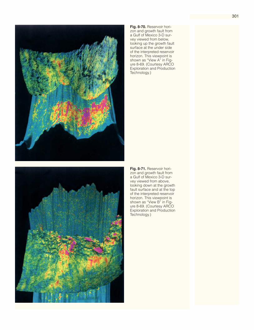
301

Fig. 8-70. Reservoir hori-zon and growth fault froma Gulf of Mexico 3-D sur-vey viewed from below,looking up the growth faultsurface at the under sideof the interpreted reservoirhorizon. This viewpoint isshown as “View A” in Fig-ure 8-69. (Courtesy ARCOExploration and ProductionTechnology.)

Fig. 8-71. Reservoir hori-zon and growth fault froma Gulf of Mexico 3-D sur-vey viewed from above,looking down at the growthfault surface and at the topof the interpreted reservoirhorizon. This viewpoint isshown as “View B” in Fig-ure 8-69. (Courtesy ARCOExploration and ProductionTechnology.)

shutters to the left and right images being displayed on the computer screen. Theresult is a very high quality stereo image, which on some workstations, can be rotatedand moved in real-time by the user.

Work is currently underway at several research labs (including Sharp Laboratoriesand British Telecom) to produce auto stereoscopic displays — displays where a stereo3-D images are perceived without any need for specialized eye wear. These displaysare still a few years away from commercial application.

Parallax is the apparent displacement of closer objects with respect to fartherobjects when observed from two different viewpoints. The effects of parallax are mostobvious when combined with motion. Driving down a highway, the objects near tothe road seem to move by more quickly than those in the distance.

Motion or animation is one of the most important cues for three-dimensional per-ception, and one of the most difficult to describe in a medium such as a printed book.The human visual system is very sensitive to small relative changes in what is beingviewed. A technique involving “flickering” between two versions of one image hasbeen used for many years in aerial photography and in astronomy to detect smallchanges in a field of view over time. Moving an observer’s viewpoint with respect toan interpreted horizon (distance, orientation, etc.) can greatly improve the under-standing of the nature of the horizon and the attribute displayed on the horizon.Motion can be used to enhance the effects of all of the other three-dimensional per-ception cues previously discussed, maximizing the visual effects of parallax, stere-oscopy, obscuration and changing the shadows cast by a light source.

The interpreter frequently needs to look at the variation of an attribute of the data(for example the trace amplitude) along a horizon surface. A multitude of horizonattributes can be extracted or calculated once a horizon has been picked. Seismicattribute analysis has been used effectively in a number of studies for fault interpreta-tion, estimation of reservoir properties, and reservoir mapping. Denham and Nelson(1986) and Dalley, et al., (1989), present good discussions of the use of horizon attrib-utes for fault interpretation. Rijks and Jauffred (1991) present an overview of attributeextraction in general.

In particular, the interpreter may be interested in the relationship between thegeometry of a three-dimensional interpreted horizon, and the variation of one (ormany) data attributes along that horizon. An understanding of this information andits implications usually must be communicated by the interpreter to others. Visual-ization techniques provide an effective means of accomplishing these goals.

The ability to understand the data, gain useful insight, and communicate thesewith others are greatly enhanced by the use of interactive 3-D visualization. Figure 8-66 is a plot of an interpreted horizon viewed from the northwest with a single “sun”or light source off to the east (left). The shape of the surface is defined by the timestructure of the interpreted horizon, and trace amplitude is mapped on the horizon incolor. Several details are now very obvious. First there are a number of small throwfaults trending roughly north to south. Most of these faults are downthrown to thewest (the right). The faults are emphasized by a combination of shadows and lowamplitude (blue) lineaments. The broad low amplitude zone clearly does not correlatewith current structure in the area (it trends roughly northeast - southwest), whereasthe strike of the axis of the anticline is northwest - southeast.

These displays can also be used to study the relationship between interpretedhorizons. The horizon in Figure 8-66 lies slightly below an unconformity. When theunconformity is picked, the data can be flattened on the unconformity. The resultingstructure is an approximation of the structure as it existed at the time depositionoccurred on the unconformity surface (Figure 8-67). In this image the horizon isbeing viewed from the northeast. This highlights the correlation between that low-amplitude zone and the crest of the Upper Cretaceous paleo-anticline. At the time ofthe unconformity, the structural trend was northeast-southwest. The low-amplitude

302

Attribute/StructureRelationships

Text continues on page 307

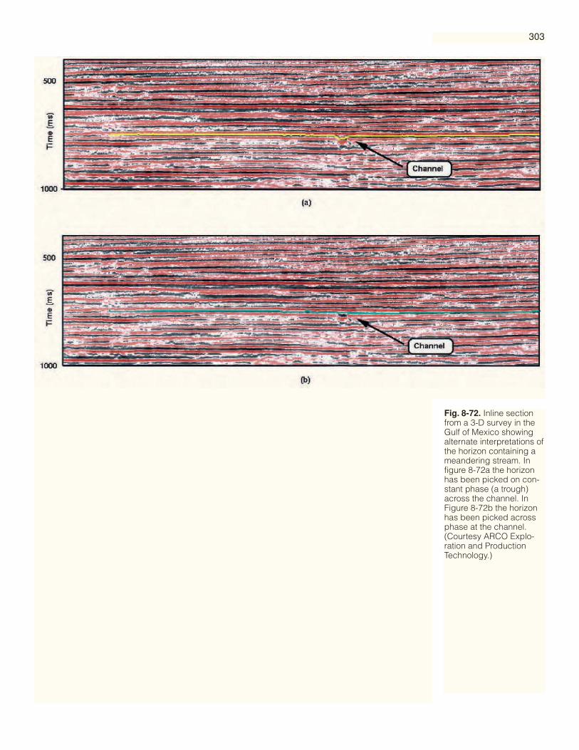
303

Fig. 8-72. Inline sectionfrom a 3-D survey in theGulf of Mexico showingalternate interpretations ofthe horizon containing ameandering stream. Infigure 8-72a the horizonhas been picked on con-stant phase (a trough)across the channel. InFigure 8-72b the horizonhas been picked acrossphase at the channel.(Courtesy ARCO Explo-ration and ProductionTechnology.)

304

Fig. 8-73. Reflection amplitudemaps at the interpreted horizoncontaining the meanderingstream in the 3-D survey in theGulf of Mexico. Figure 8-73ashows the amplitude for the hori-zon picked on constant phase,and Figure 8-73b shows theamplitude for the horizon pickedacross phase. (Courtesy ARCOExploration and ProductionTechnology.)

305

Fig. 8-74. Dip maps at the inter-preted horizon containing themeandering stream in the 3-Dsurvey in the Gulf of Mexico. Fig-ure 8-74a shows the dip for thehorizon picked on constantphase, and Figure 8-74b showsthe dip for the horizon pickedacross phase. (Courtesy ARCOExploration and ProductionTechnology.)

306

Fig. 8-75. Lighted per-spective display of thehorizon containing themeandering stream in the3-D survey in the Gulf ofMexico. In Figure 8-75athe surface and reflectionamplitude represent thehorizon picked on con-stant phase across thestream. In figure 8-75bthe surface and reflectionamplitude represent thehorizon picked acrossphase. (Courtesy ARCOExploration and Produc-tion Technology.)

(a)

(b)

zone lies along the crest of the paleo-anticline. The fact that the north-south faultsform sharp-edged boundaries to the low-amplitude zone suggests that these faultsexisted prior to the formation of the unconformity.

In Figures 8-66 and 8-67, the time-structure of horizon is used to define the shape ofthe three-dimensional surface. It is possible to use any attribute (not necessarily time)to define the shape of the three-dimensional surface while a second attribute is repre-sented by the color on the surface. In Figure 8-68, the regional or low spatial frequen-cy component of the horizon has been removed. The surface is defined by the highpass filtered horizon structure — the residual horizon, as in Figures 8-3, 8-6, 8-7 and8-8. The residual horizon will typically have its greatest non-zero values at abrupt dis-continuities such as faults. In this image we are looking at the northern half of thehorizon from the south. The ridges in the residual horizon structure associated withnorth-south trending small throw faults are clearly visible. The color in Figure 8-68still represents reflection amplitude.

Another example shows the relationship between an interpreted reservoir horizonand an associated growth fault in the Gulf of Mexico. In Figure 8-69 the horizon andfault surface are viewed from the side. Trace amplitude is shown on the surfaces incolor. From the side view it is clear that the fault surface itself has a very complexstructure. The interpreted horizon appears high near the fault, has a large depressionand then rises again farther from the fault surface.

Figure 8-70 was created by moving the viewpoint around to look up the growthfault from below the horizon. This view highlights the structural relationship betweenthe horizon and the fault surface. The fault surface has a very complex shape, withtwo major ridges with large recessed regions between and around them. The struc-ture of the horizon shows clear control by the shape of the growth fault, with largebowl shaped depressions and ridges in the horizon corresponding to the depressionsand ridges in the fault surface. Over-printed on the large scale structure of the growthfault is a finer structure of fault grooves that likely trend parallel to the direction ofmovement.

In Figure 8-71, the viewpoint has been moved to look down on the growth fault.The complex structure of the fault blocks along the ridge and in front of the growthfault surface are quite evident. Production of gas occurs in several of the high reflec-tion amplitude, isolated fault blocks adjacent to the growth fault.

In 3-D data the explorationist is provided with a unique opportunity to explore thestratigraphy of the subsurface in detail. Time slices and horizon slices allow the inter-preter to see features and detail in the data that would otherwise be missed. Three-dimensional visualization provides a means of integrating the structural and strati-graphic aspects of interpretation in detail.

Figure 4-21 is a time slice at about 750 ms from a 3-D survey in the Gulf of Mexico.Obvious features of the time slice include two major faults and a large meanderingstream. Figure 4-22 is an inline section extracted from the 3-D volume cutting perpen-dicular to the large stream. The stream appears in the seismic section as a narrowzone only a few traces wide of about 180° phase shift. One approach to interpretingthe horizon is to pick the horizon across phase - peak outside the channel, troughwithin the channel. An alternate approach to picking the horizon is to pick it at con-stant phase — that is, pick the peak both outside and within the channel. Figure 8-72is the inline from the 3-D volume, showing the horizon picked across phase (Figure 8-72a) and on constant phase (Figure 8-72b).

Figure 8-73 shows displays of the reflection amplitude at the interpreted horizonfor the pick at constant phase (Figure 8-73a), and the pick across phase (Figure 8-73b).

307

Attribute/AttributeRelationships

ComplexStructuralRelationships

Relationshipsbetween Structureand Stratigraphy

308

The dip displays of the two versions of the picked horizon are shown in Figures 8-74aand b. The stream channel is interpretable in all of the displays. For the pick acrossphase it is most evident in the amplitude display. For the pick at constant phase, thechannel is most prominent in the dip display.

There is a striking difference between the information conveyed by the two inter-pretations of the horizon when they are displayed in three dimensions. In Figures 8-75a and b, the horizon time surfaces are displayed with reflection amplitude superim-posed in color. The constant phase interpretation (Figure 8-75a) looks like a channel.The nature of the feature is obvious at a glance because of the manner in which it wasinterpreted and the way in which it is visualized. The interpretation across phase(Figure 8-75b) shows the location of the channel, but it does not convey the informa-tion as well.

The interpreter must often integrate more information than can be represented by athree-dimensional structure, a single mapped attribute, and a light source. For exam-ple, there may be effects caused by a shallower event (e.g., amplitude or frequencyshadows). In this case a visual correlation between the shallow feature and the targethorizon would provide a quick means of evaluating these effects. There are also timeswhen a visual correlation between two attributes would be important (e.g., the areaon the Top Reservoir horizon, with reflection amplitudes in color, where the con-toured cumulative production exceeds a given value). There are also situations wherea lighting and perspective do not provide sufficient visual information to understandthe complex three-dimensional nature of a horizon.

An example combining two of these cases is shown in Figures 8-76 and 8-77. TheTop Reservoir horizon structure is shown in Figure 8-76 as a 3-D surface in perspec-tive, viewed from the north at an elevation of about 45°, with a light source shining

Fig. 8-76. Lighted per-spective display of a topreservoir horizon, with thereflection amplitudeshown in color. (CourtesyARCO Exploration andProduction Technology.)

IntegratingInformation

309

down on the surface from above. Reflection amplitude is shown on the surface incolor. The structure of the surface is difficult to comprehend from this display. Someadditional visual cues are needed.

One approach to this problem, illustrated in Figure 8-77, utilizes a technique calledtexture mapping to map structure contours directly onto the horizon in 3-D. The con-tours provide the additional information necessary to understand the structure andsimultaneously allow the identification of amplitude features that occur at similardepths. Texture mapping can be used to show additional data as well. In Figure 8-77 astippling of black dots is posted on the horizon in an area where there was concernthat a shallow feature might cause an amplitude shadow at the Top Reservoir reflec-tion. The stippled zone represents the area over which the shallower feature is pre-sent. A visual assessment can now be made of the potential shadow effect on theamplitude pattern.

A second example of the use of texture mapping comes from the Pickerill Field inthe U. K. waters of the southern North Sea. A geophysical reservoir characterizationstudy (Dorn, et al., 1996) successfully derived a relationship between corrected reflec-tion amplitude at the Top Rotliegend (top reservoir) reflection and log-derived reser-voir porosity. A seismic-guided estimated porosity map was produced (Figure 8-78).The reservoir is highly faulted, and drilling indicated that at least some of the faults,sealed by diagenesis, could act as barriers to flow within the reservoir, even if thethrow along the fault was insufficient to completely offset reservoir interval. Finally, adolomite (the Plattendolomit), deposited within the Zechstein evaporite sequencewhich overlies the reservoir, is rafted in the area. As the Zechstein evaporites flowed,the dolomite fractured into rafts, so that it is present over portions of the area, and notpresent over others. The location of the Plattendolomit rafts is important becauseexploration drilling had shown that overpressure might be encountered when drillingthrough a raft.

Fig. 8-77. Lighted per-spective display of a topreservoir horizon, with thereflection amplitudeshown in color. The blackcontours are horizonstructure contours, andthe black stippled patternrepresents a region wherethe amplitudes may beattenuated due to effectsshallower in the section.(Courtesy ARCO Explo-ration and ProductionTechnology.)

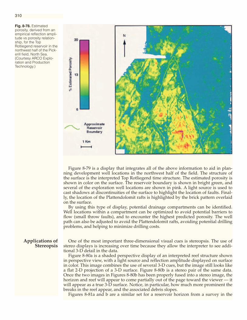
310

Figure 8-79 is a display that integrates all of the above information to aid in plan-ning development well locations in the northwest half of the field. The structure ofthe surface is the interpreted Top Rotliegend time structure. The estimated porosity isshown in color on the surface. The reservoir boundary is shown in bright green, andseveral of the exploration well locations are shown in pink. A light source is used tocast shadows at discontinuities of the surface to highlight the location of faults. Final-ly, the location of the Plattendolomit rafts is highlighted by the brick pattern overlaidon the surface.

By using this type of display, potential drainage compartments can be identified.Well locations within a compartment can be optimized to avoid potential barriers toflow (small throw faults), and to encounter the highest predicted porosity. The wellpath can also be adjusted to avoid the Plattendolomit rafts, avoiding potential drillingproblems, and helping to minimize drilling costs.

One of the most important three-dimensional visual cues is stereopsis. The use ofstereo displays is increasing over time because they allow the interpreter to see addi-tional 3-D detail in the data.

Figure 8-80a is a shaded perspective display of an interpreted reef structure shownin perspective view, with a light source and reflection amplitude displayed on surfacein color. This image combines the use of several 3-D cues, but the image still looks likea flat 2-D projection of a 3-D surface. Figure 8-80b is a stereo pair of the same data.Once the two images in Figures 8-80b has been properly fused into a stereo image, thehorizon and reef will appear to come partially out of the page toward the viewer — itwill appear as a true 3-D surface. Notice, in particular, how much more prominent thebreaks in the reef appear, and the associated debris slopes.

Figures 8-81a and b are a similar set for a reservoir horizon from a survey in the

Fig. 8-78. Estimatedporosity, derived from anempirical reflection ampli-tude vs porosity relation-ship, for the TopRotliegend reservoir in thenorthwest half of the Pick-erill field, North Sea.(Courtesy ARCO Explo-ration and ProductionTechnology.)

Applications ofStereopsis

311

southern North Sea. Figure 8-81a shows reflection amplitude in color on the top reser-voir time structure in a lighted perspective display. Figure 8-81b is a stereo pair forthe horizon from the same viewpoint. The gross aspects of the structure are clearlyevident in Figure 8-81a — the large tilted fault blocks, the north-south bounding fault,and the secondary northwest-southeast fault trend. The detail of the intra-block struc-ture only becomes obvious in the stereo display. The amplitude pattern indicated bythe arrow in Figure 8-81a, is clearly a small intra-block graben system when viewed inthe fused stereo image.

The additional information content provided to the interpreter by stereo displays issubstantially more striking with the larger stereo images that can be displayed onproperly equipped workstations. Some information that can be observed in the stereoimages could be interpreted from non-stereo displays, but the interpretation requiresmore time and effort. Other information would simply be missed without the stereodisplay.

Animation or motion of a 3-D interpretation can also play an important role ininterpretation and communication of complex structural and stratigraphic relation-ships. Three applications of motion are discussed below: changing the observer’sviewpoint, interactive three-dimensional flattening, and interactive movement of thelight source.

Motion in the form of changing the observer’s viewpoint can greatly aid interpret-ing and understanding complex 3-D structures. Motion accentuates the effects of manyof the visual cues used to perceive a 3-D object. The shifting of shadows, highlights,

Fig. 8-79. Lighted per-spective display of theTop Rotliegend time struc-ture, integrating the explo-ration well locations, theestimated porosity, thereservoir boundary andthe areas over whichthere are Plattendolomitrafts. (Courtesy ARCOExploration and Produc-tion Technology.)

Use of Motion

Text continues on page 318

312

Fig. 8-80. Lighted per-spective display of aninterpreted horizon from a3-D survey in the PermianBasin showing a reefstructure, with reflectionamplitude in color (Figure8-80a). Figure 8-80b is astereo pair for the horizon.(Courtesy ARCO Explo-ration and ProductionTechnology.)

313

Fig. 8-81. Lighted per-spective display of theinterpreted top reservoirhorizon from a 3-D surveyin the southern North SeaGas Basin, with reflectionamplitude in color (Figure8-81a). Figure 8-81b is astereo pair for the horizon.(Courtesy ARCO Explo-ration and ProductionTechnology.)

314

Fig

.8-8

2.Li

ght

ed p

ersp

ec-

tive

dis

pla

y of

an

inte

rpre

ted

Cre

tace

ous

horiz

on a

nd a

nov

erly

ing

Up

per

Cre

tace

ous

unco

nfor

mity

from

a 3

-D s

ur-

vey

in th

e so

uthe

rn N

orth

Sea

Gas

Bas

in. R

efle

ctio

nam

plit

ude

is s

how

n on

the

surf

aces

in c

olor

. (C

ourt

esy

AR

CO

Exp

lora

tion

and

Pro

-d

uctio

n Te

chno

log

y.)

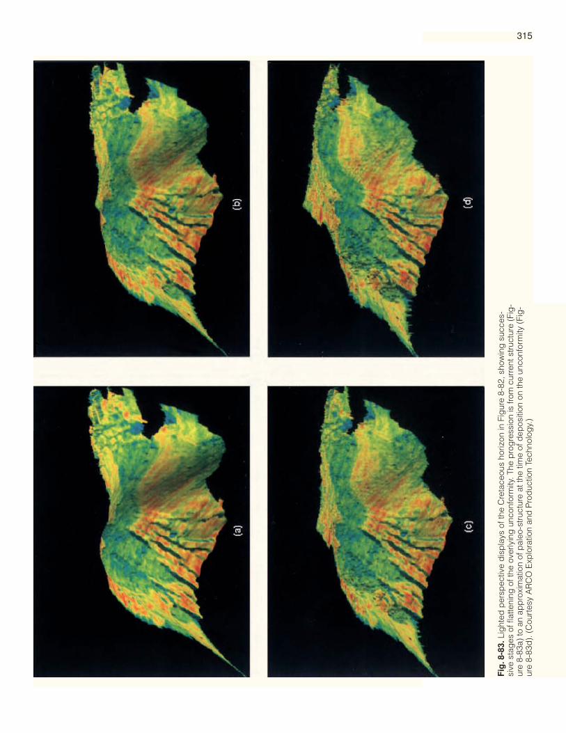
315

Fig

.8-8

3.Li

ght

ed p

ersp

ectiv

e d

isp

lays

of t

he C

reta

ceou

s ho

rizon

in F

igur

e 8-

82, s

how

ing

suc

ces-

sive

sta

ges

of f

latte

ning

of t

he o

verly

ing

unc

onfo

rmity

. The

pro

gre

ssio

n is

from

cur

rent

str

uctu

re (

Fig

-ur

e 8-

83a)

to a

n ap

pro

xim

atio

n of

pal

eo-s

truc

ture

at t

he ti

me

of d

epos

ition

on

the

unco

nfor

mity

(Fi

g-

ure

8-83

d).

(C

ourt

esy

AR

CO

Exp

lora

tion

and

Pro

duc

tion

Tech

nolo

gy.

)

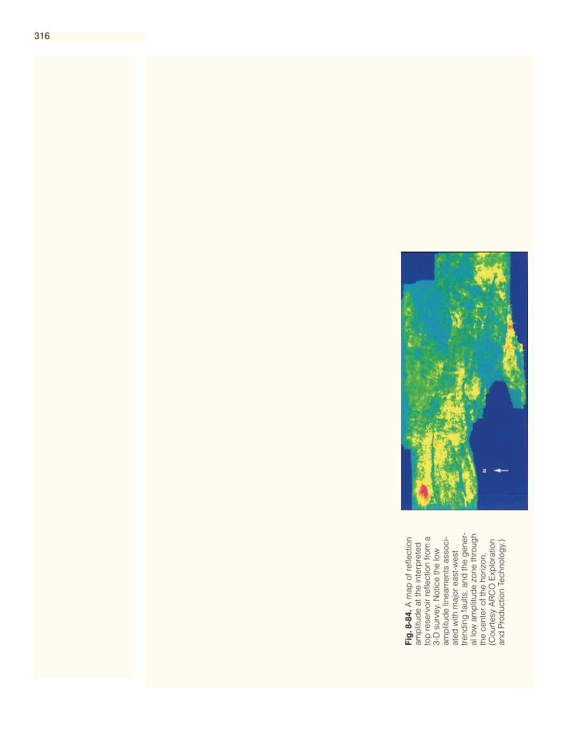
316

Fig

.8-8

4.A

map

of r

efle

ctio

nam

plit

ude

at th

e in

terp

rete

dto

p re

serv

oir

refle

ctio

n fro

m a

3-D

sur

vey.

Not

ice

the

low

amp

litud

e lin

eam

ents

ass

oci-

ated

with

maj

or e

ast-

wes

ttre

ndin

g fa

ults

, and

the

gen

er-

al lo

w a

mp

litud

e zo

ne th

roug

hth

e ce

nter

of t

he h

oriz

on.

(Cou

rtes

y A

RC

O E

xplo

ratio

nan

d P

rod

uctio

n Te

chno

log

y.)

317

Fig

.8-8

5.P

ersp

ectiv

e d

isp

lays

of r

efle

ctio

n am

plit

ude

in c

olor

on

the

inte

rpre

ted

top

rese

rvoi

r tim

e st

ruct

ure

from

a 3

-D s

urve

y vi

ewed

from

ab

ove.

The

seq

uenc

efro

m F

igur

e 8-

85a

thro

ugh

8-85

d s

how

s th

e ef

fect

s of

mov

ing

the

light

sou

rce

from

the

sout

h, to

the

wes

t, to

the

nort

h, a

nd to

the

east

of t

he h

oriz

on s

urfa

ce. (

Cou

r-te

sy A

RC

O E

xplo

ratio

n an

d P

rod

uctio

n Te

chno

log

y.)

318

changing perspective, obscuration, etc., all provide very useful visual information. Thecreation of a movie by programmed “fly-by” or path of observation through spacemay also be used to convey complex information to other technical personnel and tomanagement. This technique has been used very effectively by planetary scientists forseveral years to explore and understand the relationships between altimetry and otherremotely sensed data (e.g., view the video tape On Robot Wings — A Flight Throughthe Solar System, Finley-Holiday Films, 1992). The same approach can be used to con-vey information regarding the relationship between estimated reservoir quality andtop reservoir structure, and to highlight the location of proposed or existing wells(Dorn, et. al., 1995).

Horizon flattening is a process frequently used to understand subtle geometricrelationships between reflections. It can be a great aid in detecting and properly inter-preting angular relationships. With interpreted 3-D horizons, flattening can be per-formed interactively in three dimensions (Dorn, et. al., 1995). Figure 8-82 shows afolded and faulted horizon interpreted in a 3-D survey from the North Sea. A secondevent, an upper Cretaceous unconformity, was also interpreted (top horizon in Figure8-82). Figure 8-83 a–d shows a sequence of four images of the deeper horizon taken atdifferent stages of flattening of the unconformity. By viewing the flattening as an ani-mated movie, it is readily apparent that displacement along the faults was essentiallycomplete prior to deposition above the unconformity. Also, the subsequent deforma-tion did not reactivate these faults to any significant degree. The low-amplitude(green - blue) zone is seen to correspond to the crest of a paleo-anticline, and it is clearthat the structural trend has changed by almost 90° between Late Cretaceous time andthe present. By moving the viewpoint around while the horizon is being flattened, theinterpreter can rapidly observe and understand these relationships through the sur-vey area.

When using interactive flattening it is important to recall that this is just a flatten-ing process — a relative vertical shifting of time and amplitude. It is not true recon-struction, and should not be used as such. It can, however, provide some very usefulgeologic insight.

Figure 8-84 is a reflection amplitude map from a top reservoir horizon in a 3-D sur-vey. Interpretation of subtle reservoir faulting through the central area of the map isimportant for infill development drilling. Due to a low signal-to-noise ratio, directinterpretation of fault traces from horizon attribute maps, such as Figure 8-84, is diffi-cult.

This type of problem in fault interpretation can be addressed by the use of lighteddisplays of the 3-D horizon with horizon attributes draped on the surface in color.The value of this procedure is enhanced by the ability to move the light source (and,thus, change the shadows) in real time. The human eye can see differences in the lin-eament pattern revealed on the horizon in Figures 8-85 a-d for the light source posi-tioned to the north, south, east and west with respect to the horizon. Human vision iseven more sensitive to the subtle changes that occur as the light source is movedaround and shadows change interactively. Also, by moving the light interactively, youare much less likely to miss a subtle trend than if you restrict yourself to using a fewstatic displays.

Addy, S. K., 1998, Neural network classification method helps seismic interval inter-pretation: Oil & Gas Journal, v. 96, no. 37, p. 47-59.

Bahorich, M., and S. Farmer, 1995, 3-D seismic discontinuity for faults and strati-graphic features — the coherence cube: The Leading Edge, v.14, p. 1053-1058.

Bahorich, M., J. Lopez, N. Haskell, S. Nissen, and A. Poole, 1995, Stratigraphic andstructural interpretation with 3-D coherence: SEG 65th Annual Meeting expandedabstracts, p. 97-99.

Barnes, A. E., 1998, The complex seismic trace made simple: The Leading Edge, v. 17,p. 473-476.

Bouvier, J. D., C. H. Kaars-Sijpesteijn, D. F. Kluesner, C. C. Onyejekwe, and R. C. vander Pal, 1989, Three-dimensional seismic interpretation and fault sealing investiga-tions, Nun River Field, Nigeria: AAPG Bulletin, v.73, p. 1397-1414.

Castagna, J. P., and M. M. Backus, 1993, Offset-dependent reflectivity — theory andpractice of AVO analysis: SEG Investigations in Geophysics no. 8.

Chen, Q., and S. Sidney, 1997, Seismic attribute technology for reservoir forecastingand monitoring: The Leading Edge, v. 16, p. 445-456.

Dalley, R. M., E. C. A. Gevers, G. M. Stampfli, D. J. Davies, C. N. Gastaldi, P. A. Rui-jtenberg, and G. J. O. Vermeer, 1989, Dip and azimuth displays for 3-D seismicinterpretation: First Break, v. 7, no. 3, p. 86-95.

Denham, J. I., and H. R. Nelson, Jr., 1986, Map displays from an interactive interpreta-tion: Geophysics, v. 51, p. 1999-2006.

Dorn, G. A., M. J. Cole and K. M. Tubman, 1995, Visualization in 3-D seismic reservoirinterpretation: 5th Archie Conference, May 14-18, 1995, The Woodlands, Texas,Expanded Abstracts.

Dorn, G. A., K. Tubman, D. Cooke and R. O’Connor, 1996, Geophysical reservoir char-acterization of Pickerill Field, North Sea, using 3-D seismic and well data: To bepublished in the AAPG 3-D Seismic Atlas, edited by P. Weimer and T. Davies.

Foley, J. D., A. Van Dam, S. K. Feiner and J. F. Hughes, 1990, Computer graphics prin-ciples and practice, 2nd Edition: Addison-Wesley Publishing Co.

Hart, B. S., and R. S. Balch, 1999, Approaches to defining reservoir physical propertiesfrom 3-D seismic attributes with limited well control: an example from the JurassicSmackover Formation, Alabama: Geophysics.

Hart, B. S., 2002, Validating seismic attribute studies — beyond statistics: The LeadingEdge, v. 21, p. 1016-1021.

Haskell, N., S. Nissen, M. Hughes, J. Grindhaug, S. Dhanani, R. Heath, J. Kantorow-icz, L. Antrim, M. Cubanski, R. Nataraj, M. Schilly, and S. Wigger, 1999, Delineationof geologic drilling hazards using 3-D seismic attributes: The Leading Edge, v. 18,p. 373-382.

Hesthammer, J., 1998, Evaluation of the timedip, correlation and coherence maps forstructural interpretation of seismic data: First Break, v. 16, p. 151-167.

Hesthammer, J., 1999, Improving seismic data for detailed structural interpretation:The Leading Edge, v. 18, p. 226-247.

Hirsche, K., S. Boerner, C. Kalkomey, and C. Gastaldi, 1998, Avoiding pitfalls in geo-statistical reservoir characterization: a survival guide: The Leading Edge, v. 17, p.493-504.

Hirsche, K., J. Porter-Hirsche, L. Mewhort, and R. Davis, 1997, The use and abuse ofgeostatistics: The Leading Edge, v. 16, p. 253-260.

Hoetz, H. L. J. G., and D. G. Watters, 1992, Seismic horizon attribute mapping for theAnnerveen Gasfield, The Netherlands: First Break, v. 10, no. 2, p. 41-51.

Horkowitz, K. O., and D. R. Davis, 1996, Seismic delineation of thin sandstone reser-voirs in a shale-rich sequence using instantaneous frequency and reflection ampli-tude attributes from 3-D data, Texas Gulf Coast, in P. Weimer and T. L. Davis, eds.,AAPG Studies in Geology No. 42 and SEG Geophysical Developments Series No. 5,AAPG/SEG, Tulsa, p. 35-44.

Kalkomey, C. T., 1997, Potential risks when using seismic attributes as predictors ofreservoir properties: The Leading Edge, v. 16, p. 247-251.

319

References

Kowalik, W. S., T. M. Wissler, B. P. Dean, R. R. Brown, M. H. Hoehn, W. E. Glenn andA. Furniss, 1995, Chevron’s GeoImage — enhancement and stereoscopic viewing ofseismic horizons and other grids for improved data understanding and communi-cation: 5th Archie Conference, May 14-18, 1995, The Woodlands, Texas, ExpandedAbstracts.

Laughlin, K., P. Garossino, and G. Partyka, 2002, Spectral decomp applied to 3-D:AAPG Explorer, May 2002, p. 28-31.

Marfurt, K. J., R. L. Kirlin, S. L. Farmer, and M. S. Bahorich, 1998, 3-D seismic attribut-es using a semblance-based coherency algorithm: Geophysics, v. 63, p. 1150-1165.

N. E. Thiing Enterprises, 1993, The Magic Eye — A new way of looking at the world:Andrews and McMeel.

Oldham, A. C., and N. M. Gibbins, 1995, Lake Hope 3-D — a case study: ExplorationGeophysics, v. 26, p. 383-394.

Partyka, G., J. Gridley, and J. Lopez, 1999, Interpretational applications of spectraldecomposition in reservoir characterization: The Leading Edge, v. 18, p. 353-360.

Rijks, E. J. H., and J. C. E. M. Jauffred, 1991, Attribute extraction: An important appli-cation in any detailed 3-D interpretation study: The Leading Edge, v. 10, no. 9, p.11-19.

Schuelke, J. S., and J. A. Quirein, 1998, Validation: a technique for selecting seismicattributes and verifying results: SEG Annual Meeting Expanded Abstracts, p. 936-939.

Van de Sande, J. M. M., 1996, Prediction of reservoir parameters from 3-D seismic datafor the Zechstein 2 carbonate play in the northeast Netherlands, in P. Weimer and T.L. Davis, eds., AAPG Studies in Geology No. 42 and SEG Geophysical Develop-ments Series No. 5, AAPG/SEG, Tulsa, p. 197-204.

320

Case Histories of Three-Dimensional Seismic Surveys

This chapter presents twelve case histories demonstrating the solution of subsurfaceproblems with 3-D seismic surveys. They have been selected on the basis of their diversity: landand marine environments, U.S. and overseas locations, structural and stratigraphic objectives,development and production arenas, authors from a variety of oil companies. Furthermore,during the evolution of this book, case histories have been added but none have been removed.Accordingly, this chapter shows a more complete record and demonstrates the progression of thetechnology and the increasing sophistication of the interpretation.

No further case histories have been added for the Fourth, Fifth and Sixth Editions becauseother volumes of 3-D case histories are now available. This edition leaves the original twelvein place and has concentrated more on the techniques and methods of 3-D interpretation.However, for further case histories, the reader is thoroughly recommended to the followingsources:Allen, J. L., T. S. Brown, C. J. John, and C. F. Lobo, 1998, 3-D Seismic Case Histories from the

Gulf Coast Basin: Gulf Coast Association of Geological Societies, 339p.Pacht, J. A., R. E. Sheriff, and B. F. Perkins, 1996, Stratigraphic Analysis Utilizing Advanced

Geophysical and Wireline Technology for Petroleum Exploration and Production: GulfCoast Section, Society of Economic Paleontologists and Mineralogists Foundation, 351p.

Weimer, P., and T. L. Davis, 1996, Applications of 3-D Seismic Data to Exploration and Pro-duction: AAPG Studies in Geology, no. 42, SEG Geophysical Developments Series, no. 5, 270p.

Case History 1

East Painter Reservoir 3-D Survey, Overthrust Belt, Wyoming

Donald G. Johnson, Chevron U.S.A., Inc.

The discovery of the East Painter Reservoir field in mid-1979 led to the initiation of the first major3-D survey in the Wyoming Overthrust Belt. A 3-D survey was necessary because interpretation ofconventional 2-D seismic data over the East Painter area did not provide a sufficiently reliablepicture of the structure on the objective Triassic Nugget horizon to permit an aggressivedevelopment program. Field data for the 17 sq mi (44 sq km) East Painter 3-D survey were collectedduring the winter of 1979-80, and the final migrated sections were in hand by July 1980.

Interpretation of the final 3-D products resolved the previous structural ambiguities andshowed the East Painter structure to be continuous and almost as large as the main PainterReservoir feature. Information from the 3-D mapping allowed up to six development wells to bedrilled at one time and helped to guide the locations of the last 13 development wells — all ofthem successful. The average cost per well was between $4 and $5 million. The cost of the 3-Dsurvey was $1.6 million, which turned out to be a good value.

321CHAPTER NINE

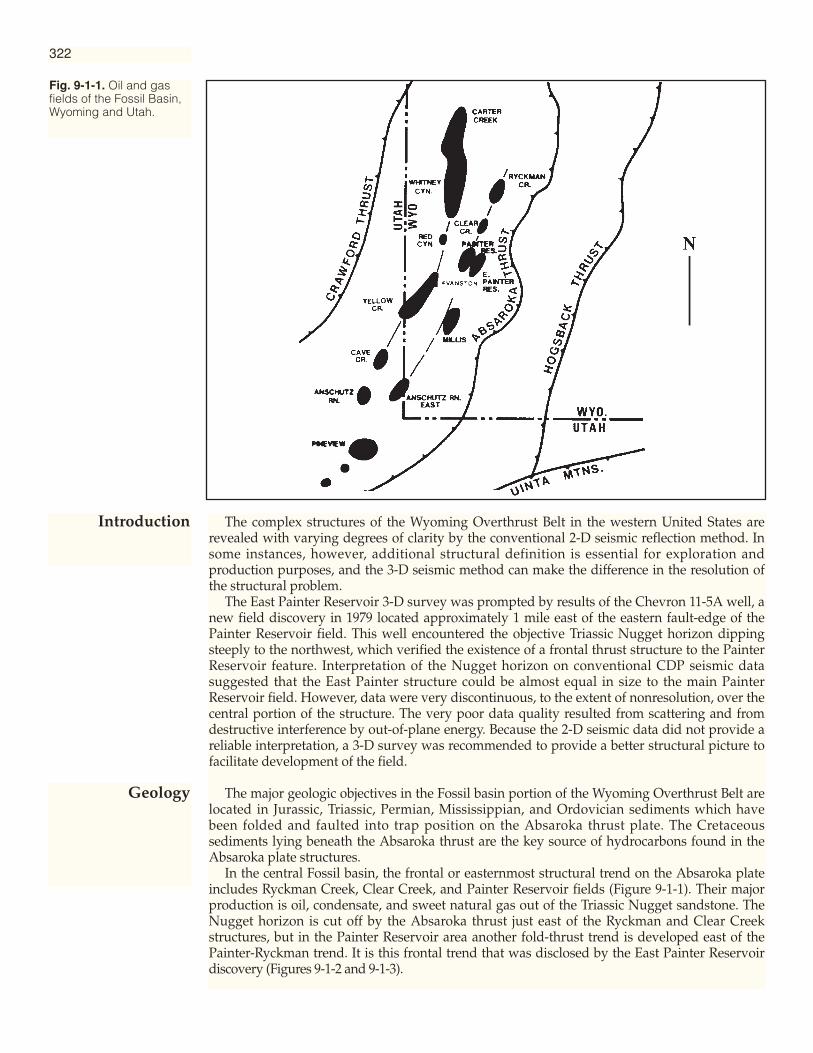
The complex structures of the Wyoming Overthrust Belt in the western United States arerevealed with varying degrees of clarity by the conventional 2-D seismic reflection method. Insome instances, however, additional structural definition is essential for exploration andproduction purposes, and the 3-D seismic method can make the difference in the resolution ofthe structural problem.

The East Painter Reservoir 3-D survey was prompted by results of the Chevron 11-5A well, anew field discovery in 1979 located approximately 1 mile east of the eastern fault-edge of thePainter Reservoir field. This well encountered the objective Triassic Nugget horizon dippingsteeply to the northwest, which verified the existence of a frontal thrust structure to the PainterReservoir feature. Interpretation of the Nugget horizon on conventional CDP seismic datasuggested that the East Painter structure could be almost equal in size to the main PainterReservoir field. However, data were very discontinuous, to the extent of nonresolution, over thecentral portion of the structure. The very poor data quality resulted from scattering and fromdestructive interference by out-of-plane energy. Because the 2-D seismic data did not provide areliable interpretation, a 3-D survey was recommended to provide a better structural picture tofacilitate development of the field.

The major geologic objectives in the Fossil basin portion of the Wyoming Overthrust Belt arelocated in Jurassic, Triassic, Permian, Mississippian, and Ordovician sediments which havebeen folded and faulted into trap position on the Absaroka thrust plate. The Cretaceoussediments lying beneath the Absaroka thrust are the key source of hydrocarbons found in theAbsaroka plate structures.

In the central Fossil basin, the frontal or easternmost structural trend on the Absaroka plateincludes Ryckman Creek, Clear Creek, and Painter Reservoir fields (Figure 9-1-1). Their majorproduction is oil, condensate, and sweet natural gas out of the Triassic Nugget sandstone. TheNugget horizon is cut off by the Absaroka thrust just east of the Ryckman and Clear Creekstructures, but in the Painter Reservoir area another fold-thrust trend is developed east of thePainter-Ryckman trend. It is this frontal trend that was disclosed by the East Painter Reservoirdiscovery (Figures 9-1-2 and 9-1-3).

Fig. 9-1-1. Oil and gasfields of the Fossil Basin,Wyoming and Utah.

Geology

322

Introduction

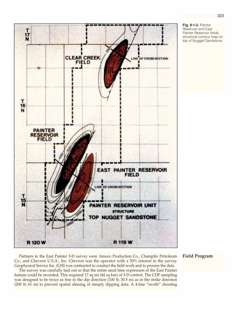
Partners in the East Painter 3-D survey were Amoco Production Co., Champlin PetroleumCo., and Chevron U.S.A., Inc. Chevron was the operator with a 50% interest in the survey.Geophysical Service Inc. (GSI) was contracted to conduct the field work and to process the data.

The survey was carefully laid out so that the entire areal time expression of the East Painterfeature could be recorded. This required 17 sq mi (44 sq km) of 3-D control. The CDP samplingwas designed to be twice as fine in the dip direction (100 ft; 30.5 m) as in the strike direction(200 ft; 61 m) to prevent spatial aliasing of steeply dipping data. A 4-line “swath” shooting

Fig. 9-1-2. PainterReservoir and EastPainter Reservoir fields,structural contour map ontop of Nugget Sandstone.

323

Field Program

method was used with dynamite in shot holes as the energy source. Where shot holes couldnot be located because of rough topography or because of close proximity to drilling wells andpipelines, substitute shot locations were carefully determined by Chevron and GSI to ensureadequate 3-D coverage. Shooting began in September 1979 and was completed in March 1980.The migrated products were received in early July 1980.

Final migrated data from the 3-D survey clearly resolved the structural configuration of theEast Painter feature (Figures 9-1-2 and 9-1-4). The resulting interpretation showed the structureto be as large as previously mapped and the questionable central portion of the structure to be

Fig. 9-1-3. PainterReservoir and EastPainter Reservoir fields,structural cross section.

324

Interpretationand Results

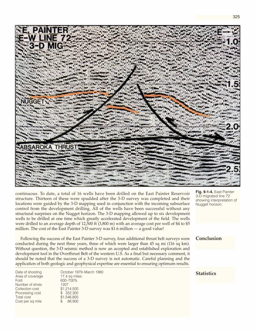
continuous. To date, a total of 16 wells have been drilled on the East Painter Reservoirstructure. Thirteen of these were spudded after the 3-D survey was completed and theirlocations were guided by the 3-D mapping used in conjunction with the incoming subsurfacecontrol from the development drilling. All of the wells have been successful without anystructural surprises on the Nugget horizon. The 3-D mapping allowed up to six developmentwells to be drilled at one time which greatly accelerated development of the field. The wellswere drilled to an average depth of 12,500 ft (3,800 m) with an average cost per well of $4 to $5million. The cost of the East Painter 3-D survey was $1.6 million — a good value!

Following the success of the East Painter 3-D survey, four additional thrust belt surveys wereconducted during the next three years, three of which were larger than 45 sq mi (116 sq km).Without question, the 3-D seismic method is now an accepted and established exploration anddevelopment tool in the Overthrust Belt of the western U.S. As a final but necessary comment, itshould be noted that the success of a 3-D survey is not automatic. Careful planning and theapplication of both geologic and geophysical expertise are essential to ensuring optimum results.

Date of shooting October 1979–March 1980Area of coverage 17.4 sq milesFold 600–700%Number of shots 1207Collection cost $1,214,500Processing cost $ 332,300Total cost $1,546,800Cost per sq mile $ 88,900

Fig. 9-1-4. East Painter 3-D migrated line 72showing interpretation ofNugget horizon.

325

Conclusion

Statistics

Case History 2

Three-Dimensional Seismic Interpretation:Espoir Field Area, Offshore Ivory CoastL. R. Grillot, P. W. Anderton, Phillips Petroleum Co. Europe-AfricaT. M. Haselton, Consultants of Tri-D, DenmarkJ. F. Dermargne, Phillips Petroleum Co. UK Ltd., England

The Espoir field, located approximately 13 km (8 mi) offshore Ivory Coast, wasdiscovered in 1980 by a joint venture comprising Phillips Petroleum Co., AGIP, SEDCOEnergy, and PETROCI. Following the discovery, a 3-D seismic survey was recorded by GSIin 1981-82 to provide detailed seismic coverage of Espoir field and adjacent features. Theseismic program consisted of 7,700 line-km of data acquired in a single survey area locatedon the edge of the continental shelf and extending into deep water. In comparison withprevious 2-D seismic surveys the 3-D data provided several improvements in interpretationand mapping including: (a) sharper definition of structural features; (b) reliable correlationsof horizons and fault traces between closely-spaced tracks; (c) preparation of detailed timecontour maps from time-slice sections; and (d) an improved velocity model for depthconversion. The improved mapping aided in the identification of additional well locations;the results of these wells compared favorably with the interpretation made prior to drilling.

The discovery well, A-1X, was drilled in approximately 1,700 ft (518 m) of water to test astructural high at the Albian unconformity level (Figure 9-2-1). The well encounteredhydrocarbon-bearing, reservoir-quality sands beneath this unconformity surface and an

Fig. 9-2-1. Location mapof 1981-82 Ivory Coast 3-D seismic surveyshowing structure ofAlbian unconformity.Contours in meters.

Introduction

326

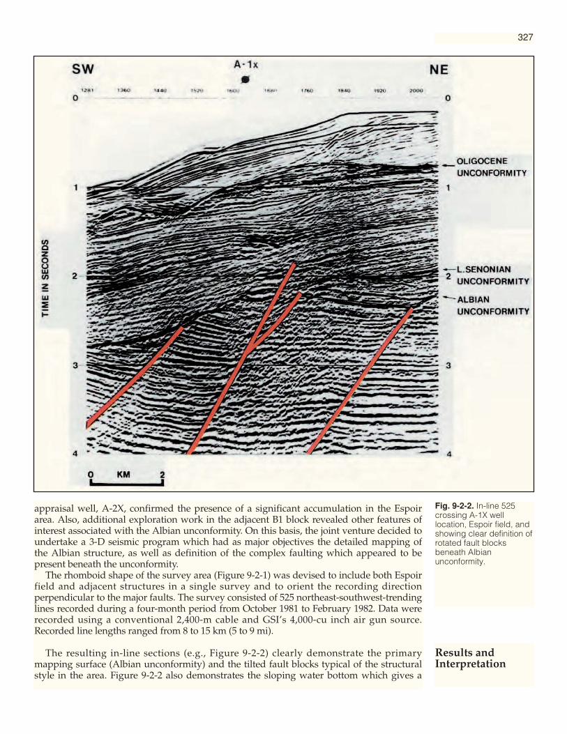
appraisal well, A-2X, confirmed the presence of a significant accumulation in the Espoirarea. Also, additional exploration work in the adjacent B1 block revealed other features ofinterest associated with the Albian unconformity. On this basis, the joint venture decided toundertake a 3-D seismic program which had as major objectives the detailed mapping ofthe Albian structure, as well as definition of the complex faulting which appeared to bepresent beneath the unconformity.

The rhomboid shape of the survey area (Figure 9-2-1) was devised to include both Espoirfield and adjacent structures in a single survey and to orient the recording directionperpendicular to the major faults. The survey consisted of 525 northeast-southwest-trendinglines recorded during a four-month period from October 1981 to February 1982. Data wererecorded using a conventional 2,400-m cable and GSI’s 4,000-cu inch air gun source.Recorded line lengths ranged from 8 to 15 km (5 to 9 mi).

The resulting in-line sections (e.g., Figure 9-2-2) clearly demonstrate the primarymapping surface (Albian unconformity) and the tilted fault blocks typical of the structuralstyle in the area. Figure 9-2-2 also demonstrates the sloping water bottom which gives a

Fig. 9-2-2. In-line 525crossing A-1X welllocation, Espoir field, andshowing clear definition ofrotated fault blocksbeneath Albianunconformity.

Results andInterpretation

327

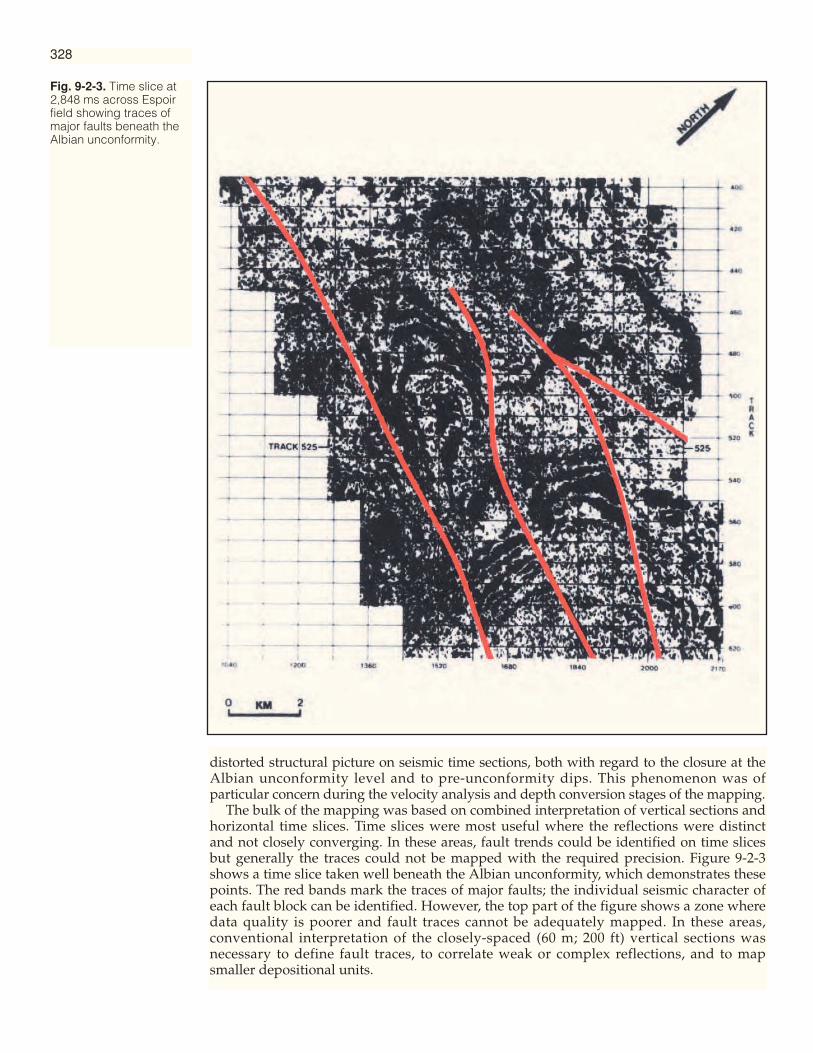
distorted structural picture on seismic time sections, both with regard to the closure at theAlbian unconformity level and to pre-unconformity dips. This phenomenon was ofparticular concern during the velocity analysis and depth conversion stages of the mapping.

The bulk of the mapping was based on combined interpretation of vertical sections andhorizontal time slices. Time slices were most useful where the reflections were distinctand not closely converging. In these areas, fault trends could be identified on time slicesbut generally the traces could not be mapped with the required precision. Figure 9-2-3shows a time slice taken well beneath the Albian unconformity, which demonstrates thesepoints. The red bands mark the traces of major faults; the individual seismic character ofeach fault block can be identified. However, the top part of the figure shows a zone wheredata quality is poorer and fault traces cannot be adequately mapped. In these areas,conventional interpretation of the closely-spaced (60 m; 200 ft) vertical sections wasnecessary to define fault traces, to correlate weak or complex reflections, and to mapsmaller depositional units.

Fig. 9-2-3. Time slice at2,848 ms across Espoirfield showing traces ofmajor faults beneath theAlbian unconformity.

328

In general, the 3-D data showed improved definition of the Albian unconformitysurface across the entire survey area. This resulted in significant mapping revisions to thetop of the reservoir interval and to changes in the extent of mapped closure over majorstructures in the area. Compared with previous efforts, the new maps showed increasedclosure at the Albian level over east Espoir together with a southward shift of thestructural crest, especially in the vicinity of well A-2X.

A particularly interesting change in mapping occurred on the feature tested by well A-4X where the erosional high on the Albian unconformity is well resolved by the 3-D data.Figure 9-2-4 shows two versions of line 358 which crosses this feature near A-4X. Thesection on the left shows data at the intermediate 2-D migration stage. Although there isevidence of an anomaly in the center of the figure at about 2.7 seconds, the feature itself isnot clear. The section on the right shows the same data after 3-D migration. Theimprovement in detail is noticeable and steeply-dipping intra-Albian reflections can beseen cutting through a flat spot which is close to a fluid contact defined in well A-4X. Theslight tilt of the flat spot is due to the sloping water bottom. The 3-D mapping confirmedthe structural isolation of the A-4X feature from the larger structure to the west.

In addition to the improvements in interpretation already discussed, benefits includedbetter definition of pre-unconformity reflections, which resulted in improved mapping ofintra-Albian horizons and better correlation across major faults. The ability to generatesections across well locations and individual features contributed to a better under-standing and interpretation of the area. In the final stages of work, the improved velocitymodel derived from the closely-spaced velocity analyses aided the preparation of depthmaps at the reservoir levels; this contributed to development of Espoir field andidentification of further appraisal locations in the area. Overall, the 3-D survey has been apositive contribution to the evaluation of the Espoir area.

Fig. 9-2-4. Comparison of2-D migration and 3-Dmigration sections acrossstructure drilled by well A-4X showing improveddefinition of erosional highon Albian unconformityand fluid contact (flatspot).

Conclusion

329

Case History 3

Field Appraisal With Three-DimensionalSeismic Surveys Offshore Trinidad

Robert M. Galbraith, Texaco Inc., Latin America/West Africa DivisionAlistair R. Brown, Geophysical Service Inc.

A consortium operated by Texaco Trinidad Inc. commenced exploration in the SouthEast Coast Consortium block offshore Trinidad in 1973. After four years of intensiveexploration, a gas/condensate discovery was announced in early 1977 on the Pelicanprospect. Later that year, in anticipation of the possible future need to site drilling/production platforms, a three-dimensional (3-D) seismic survey was recorded over theprospect. This survey resulted in improvements in seismic record quality, multipleattenuation, and fault resolution. A coordinated geologic-geophysical interpretationbased on the 3-D seismic survey, a re-evaluation of log correlations, and the use ofseismic logs differed significantly from earlier interpretations. Because of this, it isanticipated that the development of the field will need to be initiated in a differentfault block from that previously envisioned.

A second 3-D survey contiguous to the Pelican survey was recorded in 1978 over theIbis prospect. Results show significant data enhancement in the deeper part of thesection and improved fault resolution relative to previous two-dimensional (2-D)control. The 3-D interpretation has revealed a much more complex fault pattern thanoriginally mapped. Separate fault blocks will have to be individually evaluated, thusgreatly increasing exploration risk.

The republic of Trinidad and Tobago lies approximately 8 mi (13 km) off thenortheast coast of Venezuela on the continental shelf of South America. The South EastCoast Consortium was formed in 1973 to evaluate an offshore license obtained fromthe Government of Trinidad and Tobago in that year. The Consortium comprisesTexaco Trinidad Inc. (operator), Trinidad and Tobago Oil Company Ltd., and Trinidad-Tesoro Petroleum Company Ltd.

The license area lies approximately 30 mi (48 km) off the southeast coast of Trinidadin the Galeota basin. This basin covers approximately 5,000 sq mi (13,000 sq km) inwhich thick Pleistocene to upper Miocene deltaic sandstones contain hydrocarbons intraps formed in gravity-induced structures. Closures consist of large diapiric anticlinalridges and rollover features developed downthrown to major growth faults. To date,four major oil fields and four major gas fields have been discovered in the basin andrecoverable reserves have been estimated at 1 billion bbls of oil and 13+ trillion cu ft ofgas.

Exploratory drilling in the Consortium block was carried out between 1975 and 1977with a total of nine wells drilled on four separate structures. Of this total, three weredrilled on the Pelican prospect with a gas/condensate discovery declared in 1977.However, even after four years of intensive exploration, including the recording of1,400 mi (2,250 km) of 2-D seismic data, the Consortium was still unable to determine alocation for a development platform. In seeking a solution, the Consortium engagedGSI to conduct a 3-D seismic survey over the Pelican structure in 1977. Following this,the Ibis 3-D survey was recorded in 1978.

All data were recorded with 24-fold geometry along lines oriented southwest-northeast, the predominant dip direction over the block. The lines were 100 m (330 ft)apart, and the subsurface interval along each line was 33 m (108 ft). The currents in thearea were commonly 6 to 8 knots at right angles to the shooting direction, so the cabledrift was high. Continuously recorded streamer tracking data provided the location of

Introduction

330

each depth point for each shot. A common-depth-point (CDP) set was then defined asthose traces whose source-receiver midpoints fell within a bin 67 × 100 m. This limitedthe lateral subsurface smear to an acceptable level with a consequent improvement inthe stack response.

One of the reservoirs in the Pelican area occurs at the top of the Miocene. The dip atthis level between the Pelican-1 well and the northwestern boundary of the 3-D surveyarea was mapped to be 2,000 ft (610 m) on the pre-existing 2-D data. After the primaryreflections had been correctly identified using the 3-D data, less than 1,000 ft (305 m) ofdip were mapped on the north flank. This decrease in dip increased the interpreted

Fig. 9-3-1. Map ofPelican-3 sand, offshoreTrinidad, interpreted from2-D data. Contour interval250 ft (76 m).

331

Results andInterpretation

hydrocarbon-bearing area under closure by approximately 20%, thus significantlyaffecting reserve estimates and development economics.

The prime reservoir in the area is the Pelican-3 sand. Figure 9-3-1 shows the interpretedmap at this level before the 3-D survey. Figures 9-3-2 and 9-3-3 show two interpretationsmade from the 3-D survey data. While a similar difference in the northwest dip exists atthis level as was mapped at top Miocene, the principal difference between pre- and post-3-D interpretations concerns the faulting.

Initial interpretation of the logs from Pelican-1 and Pelican-3 wells indicated differentwater levels in the Pelican-3 sand. This was explained by a cross-fault separating the two

Fig. 9-3-2. Map ofPelican-3 sandinterpreted from 3-D datawith southeasternstructural closure but nothonoring water level inwell. Contour interval 250ft (76 m).

332

wells (Figure 9-3-1). The 3-D data precluded the possibility of this cross-fault. Instead, thegrowth fault has been interpreted farther northeast, thus separating the two wells at thePelican-3 sand. The impact of this on the interpreted position of the reserves is shown inFigure 9-3-2. The recommendation based on the 3-D interpretation was therefore toinitiate development drilling in a different fault block from the one proposed prior to theacquisition of 3-D control. This change in interpretation has probably saved the SouthEast Coast Consortium the expense of at least one dry hole and possibly the cost ofmislocation of a development platform.

The water level in the Pelican-3 sand in the Pelican-3 well is near 13,800 ft (4,210 m).

Fig. 9-3-3. Map ofPelican-3 sandinterpreted from 3-D datawith southeasternstratigraphic boundaryand honoring water levelin well. Contour interval250 ft (76 m).

333

Fig

. 9-3

-4.G

-LO

G v

eloc

ity s

ectio

n al

ong

cro

sslin

e 87

thro

ugh

Pel

ican

-3 w

ell s

how

ing

late

ral v

eloc

ity tr

ansi

tion

acro

ss in

ferr

edso

uthe

aste

rn r

eser

voir

bou

ndar

y.

334

The contour at this level is shown by a dashed line in Figure 9-3-2. This is 200 ft (60 m)deeper than the structural spill point of 13,600 ft (4,150 m) which, on the basis ofstructural closure alone, would control the downdip extent of the gas. An alternativeinterpretation which honors the water level in the well is shown in Figure 9-3-3. Thisinvokes a stratigraphic reservoir boundary on the southeast.

The seismic section along crossline 87, northwest-southeast through Pelican-3 well,shows a very marked character change at the Pelican-3 reservoir level southeast of thewell. This probably indicates the position of the stratigraphic boundary. This characterchange is evident on seven crosslines which intersect the boundary, and also on severalSeiscrop sections, from which its position was mapped (Figure 9-3-3).

The G-LOG* process of seismic inversion was applied to crossline 87 through Pelican-3well in an attempt to study the nature and validity of the stratigraphic boundary. Theresulting G-LOG section in color is shown in Figure 9-3-4. Generally, the higher velocitiescorrespond to the sands and the lower velocities to the shales. Cyclical sand-shaledeposition is evident above 3.0 seconds.

The simplified lithology in the well shows the Pelican-3 gas sand between 3.20 and 3.26seconds (Figure 9-3-4). There is no low velocity expression of this interval on the G-LOGsection. However, away from the well to the southeast, the correlative interval shows anabrupt lateral increase in velocity; this is interpreted as the stratigraphic reservoirboundary. Close examination of the transition suggests layering which is also observed inthe well; in the upper portion of the reservoir the transition occurs at line 70, in the nextlayer at line 79, and in the lower half of the reservoir at line 73. The magnitude of thevelocity contrast across the boundary is approximately 600 ft/sec (180 m/sec). It isconcluded that this lateral change from low to high velocity indicates the change from aporous gas-filled sand to a tight sand, in which the pores are filled with cement which isprobably clay.

Data quality has been improved. Processing took into account cable drift, a majorproblem offshore Trinidad, thus limiting subsurface smear during stack. Some deepprimary events have been observed for the first time. Because of increased data density,fault definition is excellent. Structural interpretations are more reliable with removal ofenergy from outside the plane of the section. The flexibility which permits an interpreterto generate lines in any direction is a significant benefit. The probable containment of theprincipal Pelican reserves by a stratigraphic reservoir boundary to the southeast has beensubstantially validated after a detailed study of its nature.

The 3-D results have caused major changes in the Pelican field development plans. Theinterpreted area under closure has been increased. The possibilities of drilling an initialdry hole and mislocating a development platform have been reduced due to improvedreliability of the coordinated geologic-geophysical interpretation based on the 3-D seismicsurvey and a re-evaluation of log correlations. This has had a positive effect ondevelopment economics.

The 3-D seismic method has proved to be a useful tool for field appraisal in this areaoffshore Trinidad and will be considered over other prospects prior to commitment toexpensive offshore development programs.

*Trademark of Geophysical Service Inc.

Conclusions

335

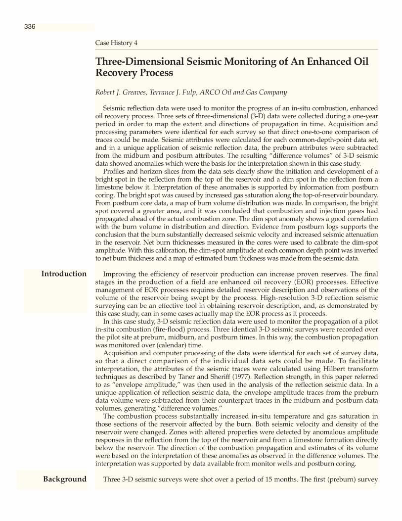
Case History 4

Three-Dimensional Seismic Monitoring of An Enhanced OilRecovery Process

Robert J. Greaves, Terrance J. Fulp, ARCO Oil and Gas Company

Seismic reflection data were used to monitor the progress of an in-situ combustion, enhancedoil recovery process. Three sets of three-dimensional (3-D) data were collected during a one-yearperiod in order to map the extent and directions of propagation in time. Acquisition andprocessing parameters were identical for each survey so that direct one-to-one comparison oftraces could be made. Seismic attributes were calculated for each common-depth-point data set,and in a unique application of seismic reflection data, the preburn attributes were subtractedfrom the midburn and postburn attributes. The resulting “difference volumes” of 3-D seismicdata showed anomalies which were the basis for the interpretation shown in this case study.

Profiles and horizon slices from the data sets clearly show the initiation and development of abright spot in the reflection from the top of the reservoir and a dim spot in the reflection from alimestone below it. Interpretation of these anomalies is supported by information from postburncoring. The bright spot was caused by increased gas saturation along the top-of-reservoir boundary.From postburn core data, a map of burn volume distribution was made. In comparison, the brightspot covered a greater area, and it was concluded that combustion and injection gases hadpropagated ahead of the actual combustion zone. The dim spot anomaly shows a good correlationwith the burn volume in distribution and direction. Evidence from postburn logs supports theconclusion that the burn substantially decreased seismic velocity and increased seismic attenuationin the reservoir. Net burn thicknesses measured in the cores were used to calibrate the dim-spotamplitude. With this calibration, the dim-spot amplitude at each common depth point was invertedto net burn thickness and a map of estimated burn thickness was made from the seismic data.

Improving the efficiency of reservoir production can increase proven reserves. The finalstages in the production of a field are enhanced oil recovery (EOR) processes. Effectivemanagement of EOR processes requires detailed reservoir description and observations of thevolume of the reservoir being swept by the process. High-resolution 3-D reflection seismicsurveying can be an effective tool in obtaining reservoir description, and, as demonstrated bythis case study, can in some cases actually map the EOR process as it proceeds.

In this case study, 3-D seismic reflection data were used to monitor the propagation of a pilotin-situ combustion (fire-flood) process. Three identical 3-D seismic surveys were recorded overthe pilot site at preburn, midburn, and postburn times. In this way, the combustion propagationwas monitored over (calendar) time.

Acquisition and computer processing of the data were identical for each set of survey data,so that a direct comparison of the individual data sets could be made. To facilitateinterpretation, the attributes of the seismic traces were calculated using Hilbert transformtechniques as described by Taner and Sheriff (1977). Reflection strength, in this paper referredto as “envelope amplitude,” was then used in the analysis of the reflection seismic data. In aunique application of reflection seismic data, the envelope amplitude traces from the preburndata volume were subtracted from their counterpart traces in the midburn and postburn datavolumes, generating “difference volumes.”

The combustion process substantially increased in-situ temperature and gas saturation inthose sections of the reservoir affected by the burn. Both seismic velocity and density of thereservoir were changed. Zones with altered properties were detected by anomalous amplituderesponses in the reflection from the top of the reservoir and from a limestone formation directlybelow the reservoir. The direction of the combustion propagation and estimates of its volumewere based on the interpretation of these anomalies as observed in the difference volumes. Theinterpretation was supported by data available from monitor wells and postburn coring.

Three 3-D seismic surveys were shot over a period of 15 months. The first (preburn) survey

Introduction

Background

336

was recorded several months previous to ignition of the combustion process. The second(midburn) survey was recorded four months after ignition, and the final (postburn) surveywas shot ten months after ignition.

The objectives of the seismic program were to (1) detect a change in seismic reflectioncharacter attributable to the combustion process, (2) determine the direction of burnfrontpropagation, and (3) determine the volume of reservoir swept by the combustion process.

The basic premise was that an increase in gas saturation in the reservoir formation wouldproduce measurable changes in reflection amplitude. Bright spots and dim spots, caused byanomalous gas concentrations, are well-known phenomena in exploration seismology.Increased gas saturation in the parts of the reservoir reached by the combustion process wasexpected to create bright spots and dim spots in the shadow zone (Sheriff, 1980). The 3-Ddata would be used to map that progression in time.

The EOR program consisted of a five-well pilot test covering a very small portion of the HoltField in north-central Texas. The test consisted of four production wells separated by 90 m (300ft) with a central injection well (Figure 9-4-1). The engineering objective was to propagate thecombustion process from the injection well radially outward, creating and flushing an increasedoil saturation zone, the oil bank, toward the production wells. Although the concept is simple,the implementation is quite difficult and is very sensitive to the details of the reservoir geology.

Fig. 9-4-1. 3-D seismicsurvey shot and receivergeometry with locations ofproduction and injectionwells.

337

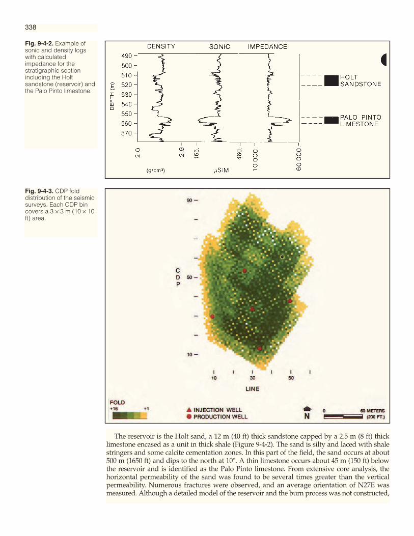
The reservoir is the Holt sand, a 12 m (40 ft) thick sandstone capped by a 2.5 m (8 ft) thicklimestone encased as a unit in thick shale (Figure 9-4-2). The sand is silty and laced with shalestringers and some calcite cementation zones. In this part of the field, the sand occurs at about500 m (1650 ft) and dips to the north at 10°. A thin limestone occurs about 45 m (150 ft) belowthe reservoir and is identified as the Palo Pinto limestone. From extensive core analysis, thehorizontal permeability of the sand was found to be several times greater than the verticalpermeability. Numerous fractures were observed, and an average orientation of N27E wasmeasured. Although a detailed model of the reservoir and the burn process was not constructed,

Fig. 9-4-2. Example ofsonic and density logswith calculatedimpedance for thestratigraphic sectionincluding the Holtsandstone (reservoir) andthe Palo Pinto limestone.

Fig. 9-4-3. CDP folddistribution of the seismicsurveys. Each CDP bincovers a 3 × 3 m (10 × 10ft) area.

338

some effects of the process were anticipated. The combustion process would primarilypropagate updip (to the south) due to the differing fluid densities. Propagation wouldprimarily occur laterally within the reservoir from the initiation points. Vertical propagationwould be limited to fractures or other natural permeability pathways. Finally, propagationmight be further guided to the southwest along fracture-induced permeability pathways.

Several factors guided the choices of acquisition parameters:

(1) the target area was very small (90 × 90 m);(2) the target was relatively shallow (500 m);(3) the data collection was to be repeated as identically as possible; and(4) the amplitudes and spatial extents of the seismic anomalies would probably be quite

small.

Simple seismic modeling based on well logs and the anticipated effect of increased gassaturation indicated that detection of the burnfront would be straightforward. However, veryhigh-resolution seismic data would be required to map the lateral extent of the process anddetermine the net burn volume. A calculation of the resolution limit was made based onWidess (1973), and the center frequency required to resolve 7.5 m (25 ft) vertically wasdetermined to be 100 Hz. The necessary resolution was felt to be achievable, given theshallow depth of the reservoir, if proper acquisition and processing techniques were applied.

Fig. 9-4-4. An example ofthe power spectra of atrace before and afterprocessing. The spectraare for the window from0.350-0.750 s whichincludes the reflectionsequence from the Holtsandstone to andincluding the Palo Pintolimestone.

Acquisition andProcessing

339

The data collection array consisted of a modified 3-D patch geometry. Figure 9-4-1 showsthe positions of shotpoints and receiver stations within the test area. This patch style ofsurvey allowed the shot pattern to be arranged as necessary, such that the CDP data werecollected with high fold over the area of primary interest (Figure 9-4-3) even though surfaceaccess was limited by buildings, wells, pipelines, etc. Furthermore, the geophones could bepermanently installed at each receiver location to guarantee that the receiver array wouldbe duplicated in each survey. A modification of the simple patch geometry was made toaccount for the migration of reflection points updip, by extending shot and receiverlocations downdip (to the north).

The receiver group spacing was 6 m (20 ft) with a single high-frequency (40 Hz) marshgeophone comprising each group. Each of the 182 receivers was buried 6 m (20 ft) belowthe surface. The 165 shotpoints were distributed along crossed lines with a 12 m (40 ft)spacing between individual shots. Each shot consisted of a 2.5 kg (3 lb) dynamite chargeburied at 23 m (75 ft). The recording system used was a 192-channel GUS-BUS withsampling interval of 1 ms and band-pass recording filters set a 50 Hz low-cut and 320 Hzantialias. The burial of both shots and receivers improved the signal-to-noise (S/N) ratio ofthe recorded data by eliminating air-wave noise and substantially reducing the amplitudeof the surface-wave noise. The 50 Hz low-cut filter was chosen at this high level to eliminatesurface-wave noise further and to preserve the dynamic range of the recording system fordigitization of the desired high-frequency signal. For recording shallow reflection seismicdata, it is especially important to eliminate surface-wave noise that can seriously degradethe quality of the shallow data window. The small, deeply buried shots, the high-frequencyphones and the low-cut filter all combined to eliminate this problem. The resultingfrequency range of the recorded data was substantially higher than the range of standardexploration seismic, as shown in Figure 9-4-4, and yet the range retained the minimum two-octave bandwidth considered necessary for high resolution.

The computer processing of the 3-D data sets used a standard sequence designed for 3-DCDP data. Throughout the processing, extra care was taken to retain true relative amplitudeand the maximum usable frequency range. The traces were gathered into 3 × 3 m (10 × 10 ft)CDP bins. The statics and normal-movement (NMO) corrections were quite small due to thesimple geologic structure and small area of the test. For more structurally complex geology, itwould have been more difficult to make proper velocity adjustments because the patchgeometry has the disadvantages of uneven fold and offset distribution. Three-dimensionalsurface-consistent statics were computed and were found to be on the order of 2 to 3 ms.Normal-moveout corrections were applied using a datumed root-mean-square (rms) velocityfunction derived from the well control. Standard spiking deconvolution was applied beforestack. A phaseless deconvolution technique was applied to balance further the usablespectrum of each stacked trace. In the final processing step, the data were migrated using anf-k migration algorithm and the velocity function derived from the sonic logs. This approachto migration was deemed adequate, given the localized area of interest and the simplevelocity structure. The frequency spectrum of a fully processed trace, windowed in thereflection zone of interest, indicates that the 40-180 Hz bandwidth of the recorded data wasenhanced during processing and the center frequency of 100 Hz was obtained (Figure 9-4-4).

As postprocessing steps, the data were properly phase-corrected using well control, andthe seismic attributes were calculated for each data set. To remove the geologic structurefrom the reflectors of interest, static adjustments were made, thereby allowing horizonviews to be sliced from the 3-D data volume. Finally, in a unique step, the preburn horizonenvelope amplitude at each level of interest was subtracted from the corresponding valuesin the midburn and postburn data volumes. The preburn data were used as the baselineseismic expression relative to which change was observed. Anomalies in the differencevolumes were then interpreted directly.

Comparison of the envelope amplitudes of the reflection event at the top of the Holt sandreservoir revealed an increase in amplitude, a bright spot, which developed after thecombustion process was initiated. In Figure 9-4-5, a north-south section, line 14, is shown as itappeared at preburn, midburn, and postburn times. The reflection from the top of the Holt

340

ObservedAnomalies—Bright Spots

sand is identified as a trough occurring at about 385 ms. At this horizon, the envelopeamplitudes at preburn time compared to midburn time show a zone of increased amplitudenear well W104, with maximum change between CDP 16 and CDP 30. By postburn time, thebright spot had increased in lateral extent from CDP 16 to CDP 36, but it had not increased inmaximum amplitude relative to midburn time.

Horizon slices at the top of the Holt sand, from the envelope amplitude difference volumes,are displayed in Figure 9-4-6. The midburn difference shows a positive amplitude anomaly inthe southwestern side of the data. This corresponds to the bright spot development observedin line 14 (Figure 9-4-5) at midburn time. Another, smaller bright spot is located to thesoutheast of the injection well at line 43, CDP 21. The difference amplitude at postburn time,Figure 9-4-6, shows that the bright spot has grown to cover most of the area within theproduction wells, the midburn peak to the southwest has shifted downdip toward well W104,and the maximum amplitude of the difference anomaly has increased by about 10 percent.

The strong reflection centered at 410 ms in line 14 (Figure 9-4-5) is identified as the PaloPinto limestone. In line 14, a slight decrease in envelope amplitude occurs in the shadow ofthe bright spot centered around CDP 22. At midburn time, the decrease in amplitude isabout 10 percent, but by postburn time, the decrease is nearly 25 percent, as marked by thechange from deep orange and red shading to yellow.

A similar display of another north-south section, line 33, in Figure 9-4-7, shows a moresubstantial dim spot. This anomaly does not coincide with any bright spot at the Holt levelat midburn time and only a modest Holt bright spot at postburn time. The dim-spotanomaly, pointed out by the arrows within the figure, is also stronger at midburn time thanat postburn time. This lack of spatial coincidence (between bright and dim spots) isimportant in the interpretation of the results as described below.

The horizon slice difference section at the Palo Pinto reflection (Figure 9-4-8) clearly showsthis anomaly. The dim spot at midburn time covers much of the pilot area with two negative-amplitude anomalies. One peak is located at the injection well, but the stronger peak liesabout 30 m (100 ft) south-southwest of the injection well. The anomalies do not coincide withbright spots in the Holt reflection. A lower amplitude lobe of the dim spot extending to thesouthwest edge of the data does correlate with the maximum bright spot observed atmidburn time. The dim spot observed at postburn time is lower in amplitude and extendsover a significantly smaller portion of the pilot area. The two peaks of the midburn anomalyhave merged into a ridge extending approximately southwest-northeast across the injectionwell with the larger area and peak of the anomaly to the southwest of the injection well.

A simple model of the in-situ combustion process, based on combustion tube experiments,was described by Tadema (1959). The combustion process within the reservoir can be dividedinto various zones, with each zone defined by its relative temperature and fluid saturations.The “combustion zone” propagates through the reservoir and is defined by maximum oxida-tion of the heaviest, or immobile, hydrocarbons. In its wake is left the “clean-burnt sand,” a hotreservoir matrix with high gas saturation. Ahead of the combustion zone are several zones atlower temperatures and with distinctive percentages of oil, water, and gases until at somedistance the original reservoir temperature and fluid mixture are encountered. Of particularinterest are (1) that the clean-burnt sand zone has been subjected to very high temperatures, and(2) that combustion gas, as well as some injection gas, are forced ahead of the combustion zone.If this model were expanded into three dimensions, it would consist of a series of concentricrings which propagate radially from the injection well. The model is quite simple and does notat all account for geologic complexities, but it is useful as a starting point for the interpretationof the seismic anomalies in terms of the physical process of in-situ combustion.

Generalizing this model to the Holt sand reservoir, it is important to point out that the Holtsand reservoir, at the initiation of the burn, had little to no gas saturation.

As stated, the first objective of the seismic program was to detect a change in reflectioncharacter attributable to the combustion process. The bright spots and dim spots are consideredtrue combustion-caused anomalies for the following reasons. First, the changes do occur in the

ObservedAnomalies —Dim Spots

Interpretation —CombustionModel

341

Interpretation —Detection

Fig. 9-4-5. Line 14, from (a) preburn, (b) midburn, and (c)postburn 3-D seismic data volumes. The reflection wiggle tracesare overlain by a color scale of the calculated envelopeamplitude. Dip was removed by static shifts before display. A

bright spot was created (see arrows) at the top of the Holtsandstone by midburn time (b), and it increases in extent bypostburn time (c). A dim spot in the reflection from the Palo Pintolimestone formed just below the peak of the bright spot.

342

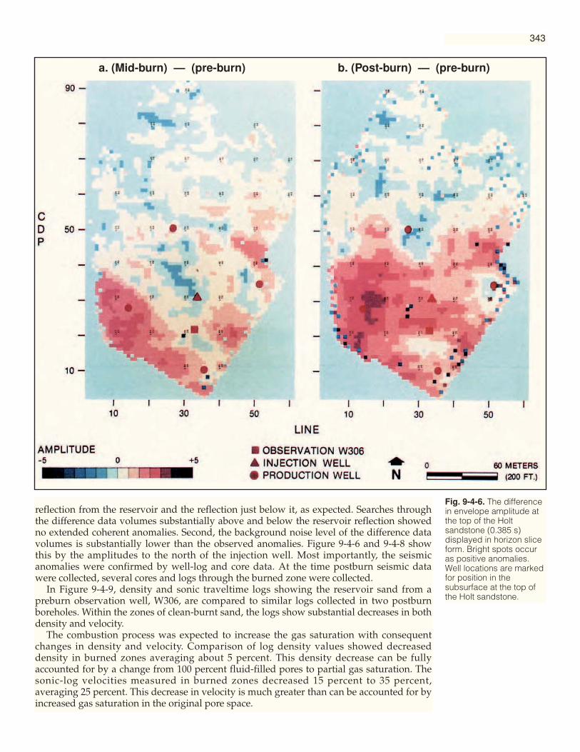
reflection from the reservoir and the reflection just below it, as expected. Searches throughthe difference data volumes substantially above and below the reservoir reflection showedno extended coherent anomalies. Second, the background noise level of the difference datavolumes is substantially lower than the observed anomalies. Figure 9-4-6 and 9-4-8 showthis by the amplitudes to the north of the injection well. Most importantly, the seismicanomalies were confirmed by well-log and core data. At the time postburn seismic datawere collected, several cores and logs through the burned zone were collected.

In Figure 9-4-9, density and sonic traveltime logs showing the reservoir sand from apreburn observation well, W306, are compared to similar logs collected in two postburnboreholes. Within the zones of clean-burnt sand, the logs show substantial decreases in bothdensity and velocity.

The combustion process was expected to increase the gas saturation with consequentchanges in density and velocity. Comparison of log density values showed decreaseddensity in burned zones averaging about 5 percent. This density decrease can be fullyaccounted for by a change from 100 percent fluid-filled pores to partial gas saturation. Thesonic-log velocities measured in burned zones decreased 15 percent to 35 percent,averaging 25 percent. This decrease in velocity is much greater than can be accounted for byincreased gas saturation in the original pore space.

Fig. 9-4-6. The differencein envelope amplitude atthe top of the Holtsandstone (0.385 s)displayed in horizon sliceform. Bright spots occuras positive anomalies.Well locations are markedfor position in thesubsurface at the top ofthe Holt sandstone.

343

a. (Mid-burn) — (pre-burn) b. (Post-burn) — (pre-burn)

344

Fig. 9-4-7. Line 33, from (a) preburn, (b) midburn, and (c)postburn 3-D seismic data volumes. The reflection wiggle tracesare overlain by a color scale of the calculated envelope

amplitude. Dip was removed by static shifts before display. A dimspot was created (see arrows) in the Palo Pinto reflection (0.410s) by midburn (b), but it decreases somewhat by postburn (c).

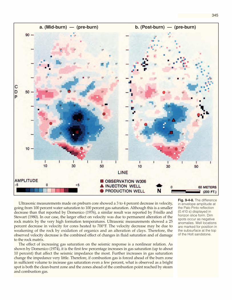
Ultrasonic measurements made on preburn core showed a 3 to 4 percent decrease in velocity,going from 100 percent water saturation to 100 percent gas saturation. Although this is a smallerdecrease than that reported by Domenico (1976), a similar result was reported by Frisillo andStewart (1980). In our case, the larger effect on velocity was due to permanent alteration of therock matrix by the very high formation temperatures. Ultrasonic measurements showed a 25percent decrease in velocity for cores heated to 700°F. The velocity decrease may be due toweakening of the rock by oxidation of organics and an alteration of clays. Therefore, theobserved velocity decrease is the combined effect of changes in fluid saturation and of damageto the rock matrix.

The effect of increasing gas saturation on the seismic response is a nonlinear relation. Asshown by Domenico (1974), it is the first few percentage increases in gas saturation (up to about10 percent) that affect the seismic impedance the most. Further increases in gas saturationchange the impedance very little. Therefore, if combustion gas is forced ahead of the burn zonein sufficient volume to increase gas saturation even a few percent, what is observed as a brightspot is both the clean-burnt zone and the zones ahead of the combustion point reached by steamand combustion gas.

345

Fig. 9-4-8. The differencein envelope amplitude atthe Palo Pinto reflection(0.410 s) displayed inhorizon slice form. Dimspots occur as negativeanomalies. Well locationsare marked for position inthe subsurface at the topof the Holt sandstone.

a. (Mid-burn) — (pre-burn) b. (Post-burn) — (pre-burn)

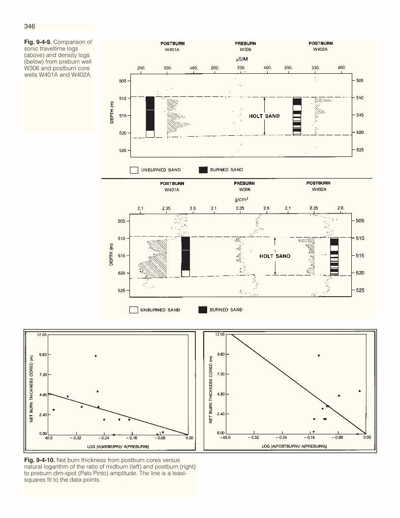
Fig. 9-4-9. Comparison ofsonic traveltime logs(above) and density logs(below) from preburn wellW306 and postburn corewells W401A and W402A.

Fig. 9-4-10. Net burn thickness from postburn cores versusnatural logarithm of the ratio of midburn (left) and postburn (right)to preburn dim-spot (Palo Pinto) amplitude. The line is a least-squares fit to the data points.

346

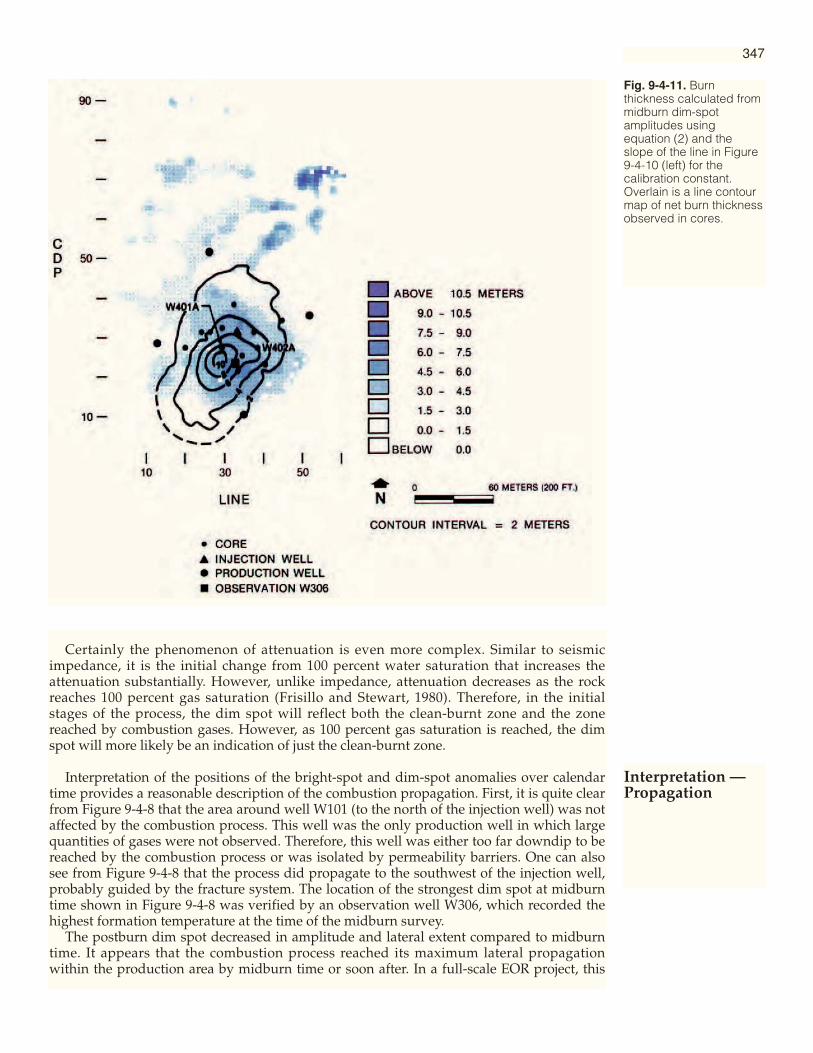
Certainly the phenomenon of attenuation is even more complex. Similar to seismicimpedance, it is the initial change from 100 percent water saturation that increases theattenuation substantially. However, unlike impedance, attenuation decreases as the rockreaches 100 percent gas saturation (Frisillo and Stewart, 1980). Therefore, in the initialstages of the process, the dim spot will reflect both the clean-burnt zone and the zonereached by combustion gases. However, as 100 percent gas saturation is reached, the dimspot will more likely be an indication of just the clean-burnt zone.

Interpretation of the positions of the bright-spot and dim-spot anomalies over calendartime provides a reasonable description of the combustion propagation. First, it is quite clearfrom Figure 9-4-8 that the area around well W101 (to the north of the injection well) was notaffected by the combustion process. This well was the only production well in which largequantities of gases were not observed. Therefore, this well was either too far downdip to bereached by the combustion process or was isolated by permeability barriers. One can alsosee from Figure 9-4-8 that the process did propagate to the southwest of the injection well,probably guided by the fracture system. The location of the strongest dim spot at midburntime shown in Figure 9-4-8 was verified by an observation well W306, which recorded thehighest formation temperature at the time of the midburn survey.

The postburn dim spot decreased in amplitude and lateral extent compared to midburntime. It appears that the combustion process reached its maximum lateral propagationwithin the production area by midburn time or soon after. In a full-scale EOR project, this

Fig. 9-4-11. Burnthickness calculated frommidburn dim-spotamplitudes usingequation (2) and theslope of the line in Figure9-4-10 (left) for thecalibration constant.Overlain is a line contourmap of net burn thicknessobserved in cores.

347

Interpretation —Propagation

knowledge would be crucial in adjusting the program to sweep the reservoir more efficiently.Although the midburn bright spot (Figure 9-4-6) also shows that the process moved to the

southwest, it does not extend back to the injection well. Therefore, the combustion gas mostlikely propagated laterally within the reservoir until it encountered a vertical permeabilitypathway which allowed the gas to stream to the top of the reservoir. Once established, thispathway also allowed the burn to move to the top of the reservoir. Up to that point, thesuccessful part of the burn was contained in the middle of the reservoir.

The postburn bright spot (Figure 9-4-6) increased in area from midburn time. A majorfault (providing the southern closure to the field) is located approximately 300 m (1000 ft) tothe south of the test. This fault probably blocked further southward propagation of thecombustion gases, forcing them back along the top of the reservoir toward the injection well.If sustained injection of gas from midburn to postburn time had continued to fuel thecombustion process, that process would have moved out beyond the production area andthe area of seismic coverage.

The final objective of this study was to estimate the volume of reservoir swept by thecombustion process. Although the data do not have the spatial resolution to map thedetailed distribution of the process, we have attempted to interpret the decreasedamplitudes in the Palo Pinto reflection as estimates of burn thickness. The mechanisms ofthe attenuation are not separable, but several factors are certainly important: pore fluidstate and interaction with the rock matrix, formation temperature, matrix velocity anddensity, and the increased reflectivity due to gas saturation in the reservoir.

A simple mathematical approach was chosen (after Waters, 1978) in which amplitude isexpressed as

(1) A = Aoe–αz,

where Ao is the initial amplitude of the propagating wavelet, α is the attenuation parameter,and z is the propagation distance. If two seismic waves are considered identical except thatone has passed through a zone Δz where the attenuation is different, then the reflectionamplitude from a level past the zone of attenuation can be compared directly to find Δz. Forthis study, observed seismic waves are the before-burn and after-burn data traces, and Δz isthe estimate of burn thickness. After taking the natural logarithms and accounting for two-way propagation, the equation becomes the linear relation

(2),

The reservoir was cored in twelve locations within the test pattern at postburn time. Thecores confirmed that the burn had occurred in somewhat vertically isolated zones withinthe reservoir. The net burn thickness observed in each core was compared to the logarithmof the ratio for appropriate seismic amplitudes at the CDPs corresponding to the bottom-hole location of each core. Figure 9-4-10 shows the comparison of net burn thickness to thelogarithm of midburn amplitude over preburn amplitude, and also the same relationshipfor postburn data. Using least-squares estimation, lines were fitted through the data pointsand forced through the origin. The slope of either of these lines could be used in equation(2) to estimate burn thickness at all other CDPs. Since the midburn data appeared to fit thesimple model better, the midburn data were used to estimate burn thickness. Thisreemphasizes the belief that burn propagation, at least within the production area, hadceased by midburn time. The postburn dim spot is more likely a map of formation damageonly, suggesting that a more complicated model is needed to explain the attenuation due toalteration of the rock fabric.

Using the slope of the midburn line in Figure 9-4-10 and equation (2), the midburn datawere converted to an estimate of net burn thickness (Figure 9-4-11). Overlain on thatestimate is a computer-generated contour map based on core data. A good correlation is

ΔzAAB A

A

B

=−

⎛⎝⎜

⎞⎠⎟

12( )

lnα α

Burn Volume

348

observed, and the correlation could have been even better if there had been core data to thesouthwest. This also implies that even without the core data for calibration, a good estimateof relative burn thickness could have been made using only the seismic data. Theobservation of seismic attenuation is a useful approach in mapping certain recoveryprocesses. Resolution could be improved utilizing borehole-to-borehole techniques.

Reflection seismic surveying can be used to monitor the progress of some EOR processes.In this case study, a fireflood process was detected, its propagation direction and extentwere determined, and an estimate of net burn volume was made.

The 3-D seismic data detected the burn zone and showed that the gas propagatedpredominately updip to the southwest. A dim spot observed in a reflector just below thereservoir level was interpreted as a map of areal extent of the burned zone. A region ofmaximum net burn thickness was located about 30 m (100 ft) from the initiation point of theburn. Comparison of the midburn and postburn dim spots led to the conclusion that themajority of the reservoir swept by the combustion process occurred in the first few monthsafter ignition. The shape, orientation, and volume of the burn interpreted from the seismicdata were confirmed by temperature monitor wells and postburn coring.

It was concluded that the attenuation increase, due to high-temperature alterations of thereservoir rock and pore fluid changes, was the best seismic indicator of the combustionprocess.

The subtraction of the baseline (preburn) data from the midburn and postburn data forinterpretation of dynamic anomalies proved to be a very powerful technique. Thesubtraction has great potential for detecting anomalous seismic response related to activereservoir processes.

The authors would like to thank ARCO Oil and Gas Company for allowing us to publishthese results. Production Engineering Research provided the financial support for thisproject. In Geophysical Support, L. F. Konty and D. R. Paschal were instrumental in surveyplanning. L. J. Hix and P. W. Wise added their expertise in data acquisition. Data processingwas designed by R. Chen and S. A. Svatek. M. L. Batzle made the petrophysicalmeasurements on core samples and provided core descriptions. J. D. Robertson contributedsupport and ideas during the interpretation of the data sets.

Domenico, S. N., 1974, Effect of water saturation on seismic reflectivity of sand reservoirencased in shale: Geophysics, v. 39, p. 759-769.

Domenico, S. N., 1976, Effect of brine-gas mixture on velocity in an unconsolidated sandreservoir: Geophysics, v. 41, p. 882-894.

Frisillo, A. L., and T. J. Stewart, 1980, Effect of partial gas/brine saturation on ultrasonicabsorption in sandstone: Journal of Geophysical Research, v. 85, p. 5209-5211.

Sheriff, R. E., 1980, Seismic stratigraphy: Boston, Massachusetts, International HumanResources Development Corporation, p. 185-198.

Tadema, H. J., 1959, Mechanism of oil production by underground combustion:Proceedings, 5th World Petroleum Congress, Section 11, p. 279-287.

Taner, M. T., and R. E. Sheriff, 1977, Applications of amplitude frequency, and otherattributes to stratigraphic and hydrocarbon determination: AAPG Memoir 26, p. 301-302.

Waters, K. H., 1978, Reflection seismology: John Wiley and Sons, p. 203-207.Widess, M. B., 1973, How thin is a thin bed?: Geophysics, v. 38, p. 1176-1180.

Acknowledgment

References

349

Conclusions

Case History 5

Impact of 3-D Seismic on Structural Interpretation atProspect Cougar

C. J. McCarthy, P. W. Bilinski, Shell Offshore, Inc.

Prospect Cougar (South Timbalier 300 Field) is an oil and gas field located in 104 m(340 ft) of water, 105 km (65 mi) south of the Louisiana shore (Figure 9-5-1). Blocks S.T.299, 300, and 301 were acquired by Shell in 1981, 1979, and 1977, respectively.

Cougar was one of Shell’s first fields to be covered by a 3-D seismic survey. Its positionnear the beginning of our 3-D learning curve, combined with the complex structure of thefield, provides an interesting illustration of the impact 3-D seismic interpretation can haveon the understanding of a field’s geology. The evolution of our understanding ofCougar ’s structure, and the impact of seismic interpretation techniques on thatunderstanding are reviewed here.

Prospect Cougar is situated in a salt-controlled basin, downthrown to a major down-to-the-south growth fault. Hydrocarbons are trapped in an anticline formed above a saltwing.

Two sands, the B and C, account for nearly all field reserves. We will concentrateexclusively on the B Sand. The B Sand is a thinly-bedded, cyclic stack of graded sand, silt,and mudstone, deposited by dilute turbidity currents. The sand package blankets thefield. Gross thickness of the package averages 50 m (160 ft). Rock properties are such thatthere is little or no reflection where the B Sand is wet; the presence of hydrocarbonsproduces a strong bright spot.

A 3-D seismic survey was acquired by Shell in 1980 (Figure 9-5-1). An area of 78 sq km(30 sq mi) was covered with an inline subsurface point spacing of 15 m (50 ft) and a linespacing of 45 m (150 ft). The total migrated area at objective depths was 26 sq km (10 sqmi).

The structural interpretation developed for lease sale is shown in Figure 9-5-2. The mapis based on a coarse, irregular grid of 2-D seismic of various vintages. The play was forturbidite sands trapped in a mildly faulted anticline. Based on this interpretation, Shellmade a successful bid of $6 million for S.T. 301.

Additional 2-D seismic was acquired in support of subsequent lease sales involvingblocks S.T. 299 and 300. At the time (1980), we recognized that the bright spot did not fitstructure. A model of a blanket turbidite sand cut by shale-filled channels was developedto explain the amplitude pattern. The essentially unfaulted interpretation is shown inFigure 9-5-3.

After successful bids for blocks S.T. 299 ($10.8 million) and 300 ($54.8 million), the 3-Dseismic survey described above was acquired to assist in developing this complexstratigraphic field. New amplitude measurements provided a detailed picture ofhydrocarbon distribution. A new structural interpretation was made using paper sectionson a relatively coarse (230 m or 750 ft) grid. This interpretation, combined with earlydevelopment drilling, indicated that faulting was more important than previouslysupposed. However, the bright spots still did not fit structure (Figure 9-5-4), sostratigraphy was assumed to play a major role in controlling hydrocarbon distribution.

At that point (1983), Shell had completed development of a photographic film-based 3-D interpretation system. Although primitive by today’s standards, the system alloweddigitized picking from enlarged profile displays and had “movie” capabilities in bothvertical section and time slice orientations. Bookkeeping features of the system finallymade it feasible to interpret every line and crossline in the survey. The tight spatial grid

Introduction

Geology

3-D Seismic

StructuralInterpretation

350

provided by the 3-D survey enabled us to map small offsets and amplitude “glitches”which had been ignored on coarser interpretation grids.

The resulting structure map (Figure 9-5-5) shows a much more complex fault pattern.Faults were recognized as controlling hydrocarbon distribution in all but one instance.The cyclic nature of the B Sand and its high shale content make even 3-m (10-ft) faultspotential seals. Because the gross thickness of the hydrocarbon column in the B Sand isgenerally at or below tuning thickness (35 m or 120 ft), local thinning of the hydrocarboncolumn associated with normal faulting produces observable amplitude decreases. Theseamplitude anomalies form linear patterns that often connect with actual event timeoffsets; in other words, they act like faults.

The fault density shown in Figure 9-5-5 was so high that it met with some disbelief. Itcertainly had a major impact on development strategy. Development drilling is nowcomplete and as many as 4 years of production data are available for some wells.Production data suggested that some reservoirs were draining areas less than shown onFigure 9-5-5, prompting reexamination of the 3-D data. The 3-D seismic data have nowbeen reprocessed and reinterpreted using a modern workstation and results from over 60wells (including sidetracks). Our current structure map (Figure 9-5-6) shows even morefaults than Figure 9-5-5. Drilling has confirmed faults picked on seismic with throws assmall as 10 m (30 ft). Faults with throws of 15 m (50 ft) can be picked very reliably onseismic.

Three-dimensional seismic surveying has played a central role in shaping our under-standing of Prospect Cougar. The field has gone from a simple, purely structural trap, to acomplex stratigraphic trap, to an even more complex structural trap. The tight spatialsampling and proper imaging provided by 3-D have been the keys to unraveling thestory. The tools and time available to the seismic interpreter have also had a major impacton our understanding of the field.

As a result of the detailed structural picture provided by the 3-D survey, a costlywaterflood program was determined to have little chance of success and consequentlywas dropped. Reexamination of the seismic data after development drilling has clarifiedwhy some wells produced as expected while others declined more rapidly thananticipated, and has provided support for new drilling and workover proposals.

The authors wish to thank Shell Offshore, Inc. and Shell Oil Company for permission topublish this material. Obviously, the interpretations described here are the work of manyindividuals in both exploration and production, too numerous to mention here. Ourpassage up the learning curve with 3-D came largely as the result of a synergistic effortamong geologists, geophysicists, and programmers, all trying to get a job done underboth time and technology constraints.

Figures begin on page 352

Conclusions

Acknowledgments

351

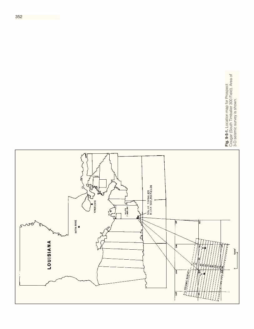
Fig

. 9-5

-1.L

ocat

ion

map

for

Pro

spec

tC

oug

ar (

Sou

th T

imb

alie

r 30

0 Fi

eld

). A

rea

of3-

D s

eism

ic s

urve

y is

sho

wn.

352

353

Fig

. 9-5

-2.I

nitia

l str

uctu

re m

ap p

rep

ared

for

first

leas

e sa

le (

1977

) fr

om 2

-D s

eism

ic g

rid.

Col

or in

dic

ates

inte

rpre

ted

hyd

roca

rbon

dis

trib

utio

n, r

ed fo

r g

as a

nd g

reen

for

oil.

Sol

idb

lack

sq

uare

s sh

ow p

rese

nt lo

catio

n of

pla

tform

s.

354

Fig

. 9-5

-3.S

truc

ture

map

from

den

ser

2-D

sei

smic

grid

afte

r d

rillin

g th

ree

exp

lora

tory

wel

lsin

S.T

. 301

(19

79).

355

Fig

. 9-5

-4.S

truc

ture

map

bas

ed o

n co

arse

-grid

inte

rpre

tatio

n of

3-D

dat

a af

ter

dril

ling

six

dev

elop

men

t wel

ls fr

om th

e S

.T. 3

00 p

latfo

rm (

1982

).

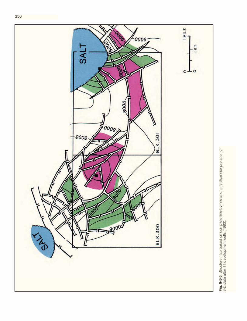
356

Fig

. 9-5

-5.S

truc

ture

map

bas

ed o

n co

mp

lete

line

-by-

line

and

tim

e sl

ice

inte

rpre

tatio

n of

3-D

dat

a af

ter

11 d

evel

opm

ent w

ells

(19

83).

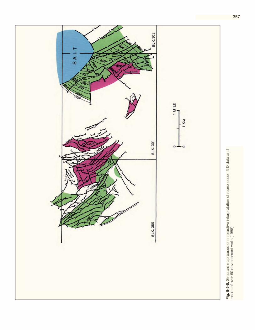
357

Fig

. 9-5

-6.S

truc

ture

map

bas

ed o

n in

tera

ctiv

e in

terp

reta

tion

of r

epro

cess

ed 3

-D d

ata

and

resu

lts o

f ove

r 60

dev

elop

men

t wel

ls (

1988

).

Case History 6

3-D Seismic Interpretation of an Upper Permian GasField in Northwest Germany

H. E. C. Swanenberg, F. X. Fuehrer, BEB Erdgas und Erdoel GmbH

In northwest Germany, sour gas is produced from Zechstein (Upper Permian)carbonates in a number of mainly medium-sized fields. A 3-D survey was acquired in1985 to optimize drilling in the Goldenstedt field and some smaller adjacent fields (Figure9-6-1). Recent appraisal drilling has proved significantly more potential than originallyassumed in this area of complex structure and facies. Total reserves are currentlyestimated at 0.5 tcf of sour gas with an H2S content varying between 7 and 26%.

Structural definition and resolution of the target horizon at 3500 to 4000 m depth(corresponding to 2.2 to 2.4 sec two-way traveltime) is severely influenced by lateralvelocity variations in the overburden, which complicated processing and interpretation ofthe survey. Despite nominally lower coverage than regular 2-D, the superiority of 3-Ddata significantly enhanced structural control. Some information on the reservoir was alsoobtained from reflection amplitudes. The 3-D data set thus revealed details of the tectono-depositional framework not observed on previous 2-D data.

Core data and modern lithologic log interpretation techniques in conjunction withdipmeter data indicate that the Zechstein carbonates in the Goldenstedt area weredeposited during a transgressional cycle of the Zechstein sea in a tidal flat environmentwith tidal channels influenced by syndepositional faulting. In the shallow, low-energyenvironment, mainly mudstones together with anhydrite were deposited with hardly anyporosity and permeability. In the higher-energy environment, grainstones were producedthat are now found mainly within the middle and upper parts of the sequence,intercalated within mudstones. In the tidal channels, the best reservoir facies (with up to100 m of pure grainstones) accumulated due to continuous subsidence resulting from thesyndepositional faulting. Early diagenesis has altered the originally deposited limestonesinto dolomites. Because of the variations in primary facies and diagenetic overprinting,net thicknesses in Goldenstedt now vary between 5 and 100 m, porosities range from verylow to 16%, and permeabilities reach 320 md. Fortunately, in the tight reservoir parts,fractures usually enhance permeability. The Zechstein carbonates are directly overlain by30 to 80 m of anhydrite and several hundred meters of Zechstein salt. During theMesozoic and Cenozoic, sedimentation in the area continued, locally governed by varioustectonic events.

The Goldenstedt area straddles the boundary between a relatively stable block in thenorth and the inverted Lower Saxony Basin (LSB), a large intracratonic inversionstructure in northwest Europe (Betz et al., 1987). In this part of the LSB (the edge of whichis visible at the southern end of the north-south seismic line in Figure 9-6-2), and in thesimilarly inverted “Goldenstedt graben,” a smaller satellite structure just north of it,Lower Cretaceous sediments accumulated during an extensional phase. During asubsequent compressional phase in the Late Cretaceous, these structures were inverted.Concomitantly, thick Upper Cretaceous sequences were deposited in the adjacent rimsynclines. During these tectonic phases the Zechstein salt decoupled the Mesozoic fromthe Paleozoic so that their respective structural styles are quite different.

Introduction

DepositionalModel, Diagenesis,

Reservoir Quality

Structural Setting

358

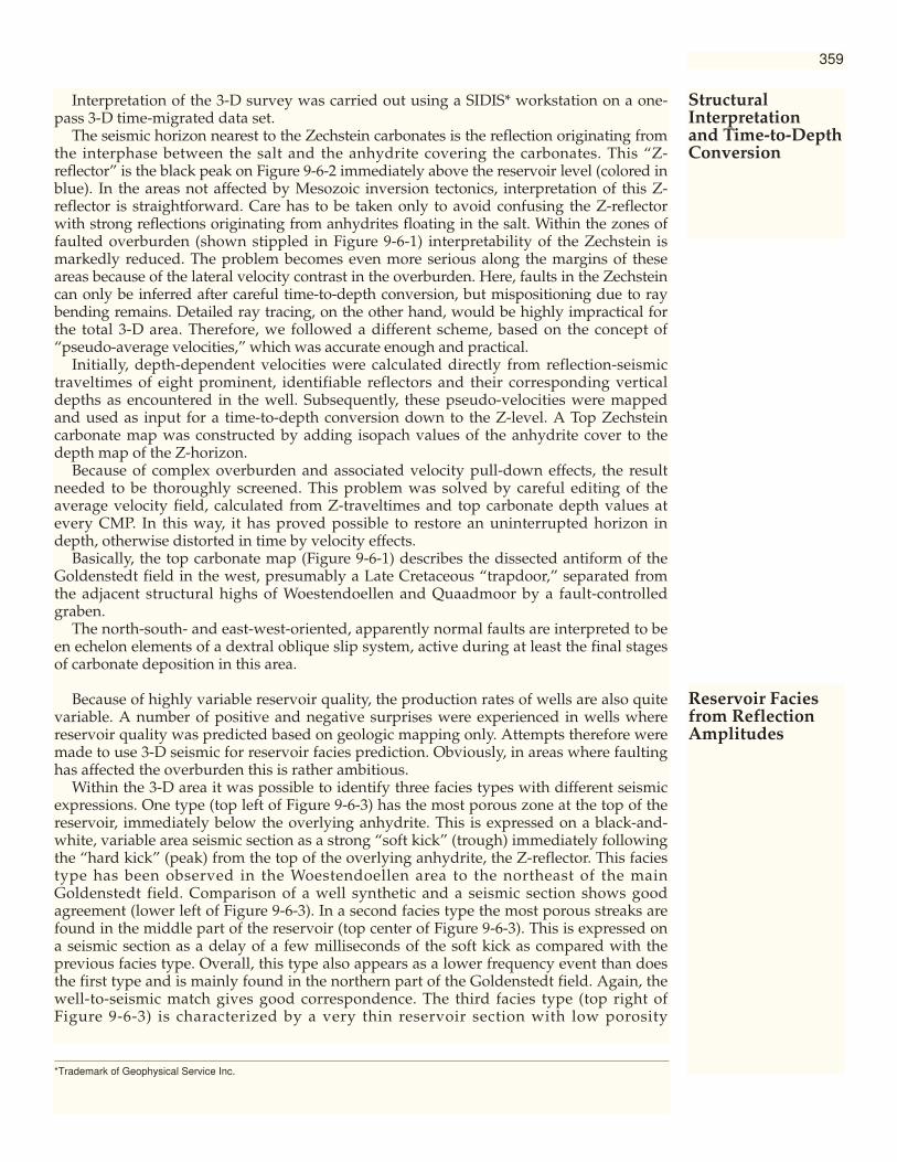
Interpretation of the 3-D survey was carried out using a SIDIS* workstation on a one-pass 3-D time-migrated data set.

The seismic horizon nearest to the Zechstein carbonates is the reflection originating fromthe interphase between the salt and the anhydrite covering the carbonates. This “Z-reflector” is the black peak on Figure 9-6-2 immediately above the reservoir level (colored inblue). In the areas not affected by Mesozoic inversion tectonics, interpretation of this Z-reflector is straightforward. Care has to be taken only to avoid confusing the Z-reflectorwith strong reflections originating from anhydrites floating in the salt. Within the zones offaulted overburden (shown stippled in Figure 9-6-1) interpretability of the Zechstein ismarkedly reduced. The problem becomes even more serious along the margins of theseareas because of the lateral velocity contrast in the overburden. Here, faults in the Zechsteincan only be inferred after careful time-to-depth conversion, but mispositioning due to raybending remains. Detailed ray tracing, on the other hand, would be highly impractical forthe total 3-D area. Therefore, we followed a different scheme, based on the concept of“pseudo-average velocities,” which was accurate enough and practical.

Initially, depth-dependent velocities were calculated directly from reflection-seismictraveltimes of eight prominent, identifiable reflectors and their corresponding verticaldepths as encountered in the well. Subsequently, these pseudo-velocities were mappedand used as input for a time-to-depth conversion down to the Z-level. A Top Zechsteincarbonate map was constructed by adding isopach values of the anhydrite cover to thedepth map of the Z-horizon.

Because of complex overburden and associated velocity pull-down effects, the resultneeded to be thoroughly screened. This problem was solved by careful editing of theaverage velocity field, calculated from Z-traveltimes and top carbonate depth values atevery CMP. In this way, it has proved possible to restore an uninterrupted horizon indepth, otherwise distorted in time by velocity effects.

Basically, the top carbonate map (Figure 9-6-1) describes the dissected antiform of theGoldenstedt field in the west, presumably a Late Cretaceous “trapdoor,” separated fromthe adjacent structural highs of Woestendoellen and Quaadmoor by a fault-controlledgraben.

The north-south- and east-west-oriented, apparently normal faults are interpreted to been echelon elements of a dextral oblique slip system, active during at least the final stagesof carbonate deposition in this area.

Because of highly variable reservoir quality, the production rates of wells are also quitevariable. A number of positive and negative surprises were experienced in wells wherereservoir quality was predicted based on geologic mapping only. Attempts therefore weremade to use 3-D seismic for reservoir facies prediction. Obviously, in areas where faultinghas affected the overburden this is rather ambitious.

Within the 3-D area it was possible to identify three facies types with different seismicexpressions. One type (top left of Figure 9-6-3) has the most porous zone at the top of thereservoir, immediately below the overlying anhydrite. This is expressed on a black-and-white, variable area seismic section as a strong “soft kick” (trough) immediately followingthe “hard kick” (peak) from the top of the overlying anhydrite, the Z-reflector. This faciestype has been observed in the Woestendoellen area to the northeast of the mainGoldenstedt field. Comparison of a well synthetic and a seismic section shows goodagreement (lower left of Figure 9-6-3). In a second facies type the most porous streaks arefound in the middle part of the reservoir (top center of Figure 9-6-3). This is expressed ona seismic section as a delay of a few milliseconds of the soft kick as compared with theprevious facies type. Overall, this type also appears as a lower frequency event than doesthe first type and is mainly found in the northern part of the Goldenstedt field. Again, thewell-to-seismic match gives good correspondence. The third facies type (top right ofFigure 9-6-3) is characterized by a very thin reservoir section with low porosity

Reservoir Faciesfrom ReflectionAmplitudes

359

StructuralInterpretationand Time-to-DepthConversion

*Trademark of Geophysical Service Inc.

mudstones only. A strong soft kick following the Z-reflector cannot be found. This faciestype is encountered in the southern part of the Goldenstedt field.

In order to visualize these observations over the whole 3-D area, horizon slices wereproduced at successive intervals below and parallel to the Z-reflector. Those for 8- and 20-ms delay are shown color coded in Figures 9-6-4 and 9-6-5, respectively. The 8-ms horizonslice (Figure 9-6-4) shows the strong soft kick characteristic of the first type as a distinctdeep-blue event. By comparing Figures 9-6-4 and 9-6-1, it is apparent that this deep-blueevent occurs in Woestendoellen, as well as in a number of other areas. In the Goldenstedt-N and Goldenstedt-S subareas, the reservoir reflection has not yet been reached at thisparticular time delay. Part of the amplitude variation over this horizon slice, however, isto be ascribed to signal deterioration and interference/absorption effects that are notrelated to reservoir development.

At 20 ms below the Z-reflector (Figure 9-6-5) the second facies type is clearly displayedin the Goldenstedt-N subarea, again by a distinct deep-blue event. Part of the time delay,however, is due to increased thickness of the overlying anhydrite. In the southern part ofGoldenstedt a strong soft kick that would appear in dark blue colors cannot generally befound, either on the 20-ms horizon slice or on any other.

Using seismic data for reservoir prediction in areas of complex facies developmentrequires detailed analysis of composite wavelet characteristics, because changes in thereflection shape cannot usually be attributed to variations of a single parameter of thereservoir only. Nevertheless, this example shows that even in rather complex cases,horizon slices can facilitate the study of the spatial distribution of wavelet characteristics.These studies can then be used to optimize well positioning in order to maximizeproduction rates and minimize the number of wells required in field development.

Goldenstedt and surrounding fields are operated by BEB Erdgas und Erdoel,Hannover, an affiliate of Shell and Exxon, holding two-thirds of the interest in the fields.One-third is held by Mobil Oil. The authors are indebted to the managements of BEB andMobil Oil for permission to publish this case history.

Betz, D., F. Fuehrer, G. Greiner, and E. Plein, 1987, Evolution of the Lower Saxony Basin:Tectonophysics, v. 137, p. 127-170.

Figures begin on page 361

Conclusion

Acknowledgment

References

360

Fig

. 9-6

-1.S

truc

tura

l map

of t

he G

old

enst

edt a

rea.

Con

tour

s in

met

ers

bel

ow s

ea le

vel.

Stip

ple

d z

ones

ind

icat

e ar

eas

whe

re r

esol

utio

n an

d ti

me

to d

epth

con

vers

ion

are

affe

cted

by

stro

ngly

tect

oniz

ed o

verb

urd

en.

361

362

Fig

. 9-6

-2.N

orth

–sou

th-t

rend

ing

sei

smic

sec

tion

show

ing

inve

rsio

n te

cton

ics

in th

eov

erb

urd

en. R

eser

voir

carb

onat

es, a

t 2.2

to 2

.4 s

ecs

refle

ctio

n tim

e, a

re in

dic

ated

in b

lue.

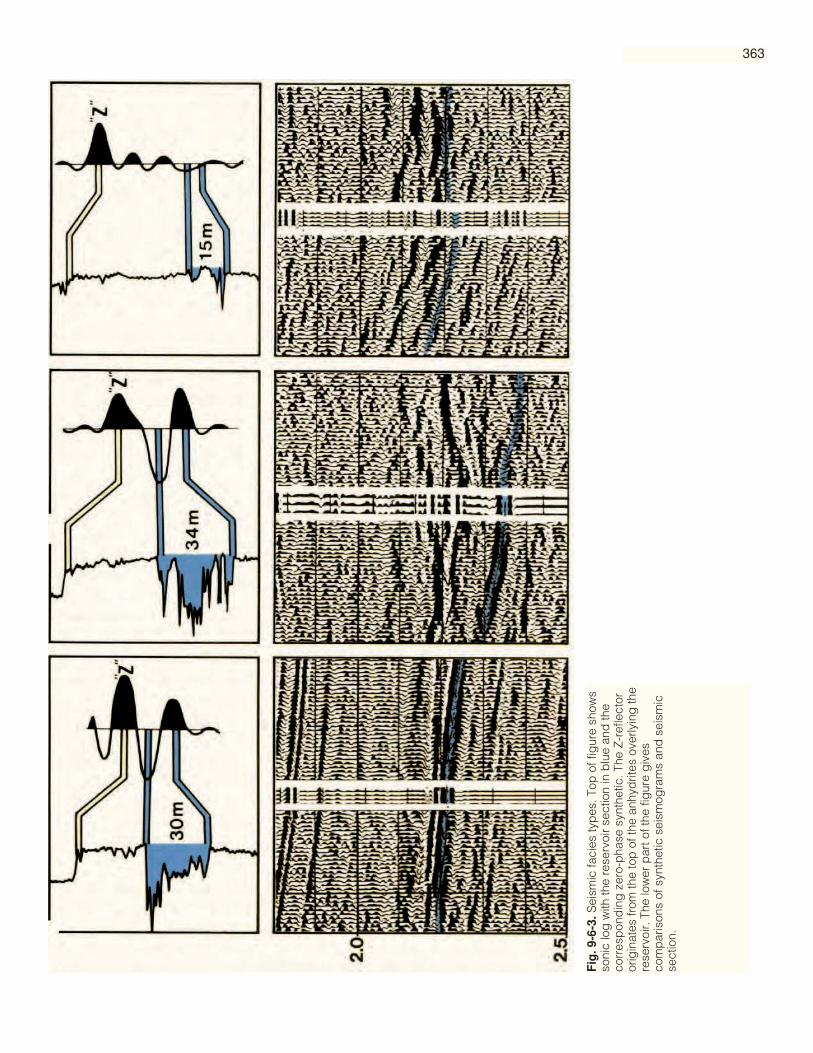
363

Fig

. 9-6

-3.S

eism

ic fa

cies

typ

es. T

op o

f fig

ure

show

sso

nic

log

with

the

rese

rvoi

r se

ctio

n in

blu

e an

d th

eco

rres

pon

din

g z

ero-

pha

se s

ynth

etic

. The

Z-r

efle

ctor

orig

inat

es fr

om th

e to

p o

f the

anh

ydrit

es o

verly

ing

the

rese

rvoi

r. T

he lo

wer

par

t of t

he fi

gur

e g

ives

com

par

ison

s of

syn

thet

ic s

eism

ogra

ms

and

sei

smic

sect

ion.

364

Fig

. 9-6

-4.H

oriz

on s

lice

with

col

or-c

oded

am

plit

udes

at 8

ms

bel

ow th

e Z

-ref

lect

or. D

eep

blu

ere

pre

sent

s re

flect

ion

amp

litud

es o

f a s

tron

g “

soft

kick

” (t

roug

h) in

dic

atin

g p

oros

ity in

the

upp

erp

art o

f the

res

ervo

ir.

Case History 7

Seismic Data Interpretation for Reservoir Boundaries,Parameters, and Characterization

William L. Abriel, Roger M. Wright, Chevron U.S.A. Inc.

Three-dimensional mapping of seismic data revealed a prospect not existing on the1000′ 2-D grid. A bright spot was reviewed downdip of an abandoned competitor wellthat had apparently been faulted out. Normal 3-D mapping resulted in a new wellproposal, but results from interactive workstation analysis moved the location downdip.Detailed structural and amplitude analyses revealed the presence of complexstratigraphic changes within the prospective reservoir, which were then avoided in asuccessful discovery well. Predictions of net pay and reservoir connectivity wereconfirmed. Future management of this reservoir will also be better served with combinedgeological, engineering, and geophysical analyses.

An offshore area in the Gulf of Mexico was reviewed for prospects, based on a 305-m(1000-ft) 2-D seismic grid and available well data (Figure 9-7-1). No clear bright spotswere observed on seismic data, and the abandoned competitor well was not encouraging(Figure 9-7-2) because of the shaly sands encountered. The area was later covered by 3-Dseismic data as part of a larger survey, and the subsequent structural evaluation was quitedifferent (Figure 9-7-3).

The 3-D survey was conducted in 1983 with an airgun source and a 3000-m streamer of120 groups at 25-m spacing. Lines were shot at 70-m and interpolated to 35-m. 3-Dprocessing consisted of relative amplitude scaling, zero-phase deconvolution, dipselective moveout, and finite difference 2-pass migration. Subsurface 3-D bins covered anarea 12.5-m by 35-m.

A map was constructed from the 3-D data using wiggle trace variable area plots(Figure 9-7-4) and a Seiscrop table. Each line was reviewed, the faults tied, and thehorizons of interest mapped. Although the area has fairly low dip, the 3-D data changedthe fault pattern significantly from the 2-D map and also revealed large, undetected brightspot zones. As a result, a well proposal was considered on the 3-D line east–west throughthe abandoned #1 well to test the large bright spot downdip (Figure 9-7-4). Theinterpretation of the data suggested that the #1 well was faulted in the stratigraphicinterval, and that the shaly gas sands of questionable productivity found in that well didnot represent the overall stratigraphy of the downdip reservoir. Geologists and engineersreviewed the prospect with geophysicists and determined a location about 305 m (1000 ft)west of the #1 well. Gas was anticipated in a strong water-drive reservoir.

Drilling could have proceeded at this point, but more time was allocated to reviewthe 3-D data on an interactive workstation. The review showed some very importantdetails that had bearing on the well proposal. Careful attention to color densityrepresentation of the lines (Figure 9-7-5) was possible with the workstation. Theamplitudes of the troughs (negative acoustic impedance contrast) of the zero-phase datawere displayed as increasing white-yellow-red, whereas the peaks (positive acousticimpedance contrast) were increasing black-green-blue. Variations in the amplitude ofthe bright spot could then be seen that were not visible in the amplitude-clipped black-and-white sections.

A simple review of the line containing the proposed #2 well showed it to be targeted ata slightly weaker amplitude spot (Figure 9-7-5). Past drilling experience in other areas hadshown this to be a less than optimum site for development wells. The position of the #2well on the 3-D structure map was at the north tip of a north-south fault, the throw of

Introduction

Initial 3-DMapping

InteractiveWorkstation

Review

366

which could not be resolved by the 3-D data. A comprehensive review of the seismic datawas in order.

All of the lines in the bright spot area were reviewed in lines, crosslines, time slices,and in cubes (Figure 9-7-6). By picking the maximum amplitude of the first trough, astructure map was made on the top of the potential reservoir (Figure 9-7-7). The map ofthe bright spot reflects an updip termination against a fault, and several potential faults,within the anomaly. Structural variations along strike on the order of 15 m (50 ft)appeared to reflect potential compaction features, suggesting variations in sanddistribution. After reviewing the lines in detail, it was determined that the potentialreservoir was probably composed of overlapping sand units on a common water contact.Line 123 (Figure 9-7-8) showed a particularly good example of possible multiple sandlobes as opposed to a faulted uniform sand. The small faults mapped on black-and-whitesections are thus more likely to be stratigraphic changes.

To better understand the distribution of the quality of the sands, the amplitudes of thereflecting interfaces were tracked, corrected for tuning effects, and represented in mapform (Figure 9-7-9). In addition, a net pay map was generated (Figure 9-7-10). Theprocedures used were an extension of more established methods (see Chapter 7, andBrown et al., 1984). It is reasonable in this geologic area to expect the higher, detunedamplitude zones to represent thicker effective sands, and this is generally represented inthe net pay map.

The resulting maps showed that the proposed #2 well lay in a very weak amplitudearea relative to the rest of the major fault block. Net pay estimates here were not veryfavorable. A real danger existed that the well would be drilled in a shaly zone and wouldnot effectively drain the potential reservoir. The connectivity of the sands appeared to bemuch better downdip, although considerable variation existed there as well. It was notsimple to accept the movement of this potential gas well downdip. If the sands were to beuniform in distribution, the net recoverable would be less. Even so, after the seismicinterpretation was considered along with other factors affecting the proposal, a new targetwas considered west (downdip) of the original proposed #2 (see Figure 9-7-10).

The #2 well was finally drilled after this extensive review, and the resulting well was asuccess (Figure 9-7-11). The #2 well was predicted to have much better sand characteristicsthan the #1 well and 17.7 m (58 ft) of effective pay. The #2 well actually logged 18.3 m (60 ft)of effective pay, and showed that the #1 well was in fact significantly faulted in its uppersection of sands. Production tests confirm that the well is in a reasonably large and well-connected reservoir.

Additional wells may be considered in the future for this reservoir. The productioncharacteristics of the #2 well may require more wells to drain all of the reserves effectively.Simple reservoir simulations are now possible using some of the data already generatedfrom the geophysical workstation, especially the reservoir boundaries and net pay.Porosity values scaled to the #1 and #2 wells can also be generated from the amplitudedata. To date, the reservoir is considered to be on a common water contact, but theapparent stratigraphic changes within the unit may potentially be permeability barriers(Figure 9-7-12).

The authors thank Chevron management for their support and permission to publishthese data. Special recognition is intended for David Smith of Chevron, Eastern Region,who worked with the geologists, geophysicists, and engineers to help get the successfulwell drilled.

Brown, A. R., R. M. Wright, K. D. Burkart, and W. L. Abriel, 1984, Interactive seismicmapping of net producible gas sand in the Gulf of Mexico: Geophysics, v. 49, p. 686-714.

Figures begin on page 368

Detailed DigitalStructure andAmplitude

Revised WellProposal

FutureReservoirManagement

Acknowledgments

References

367

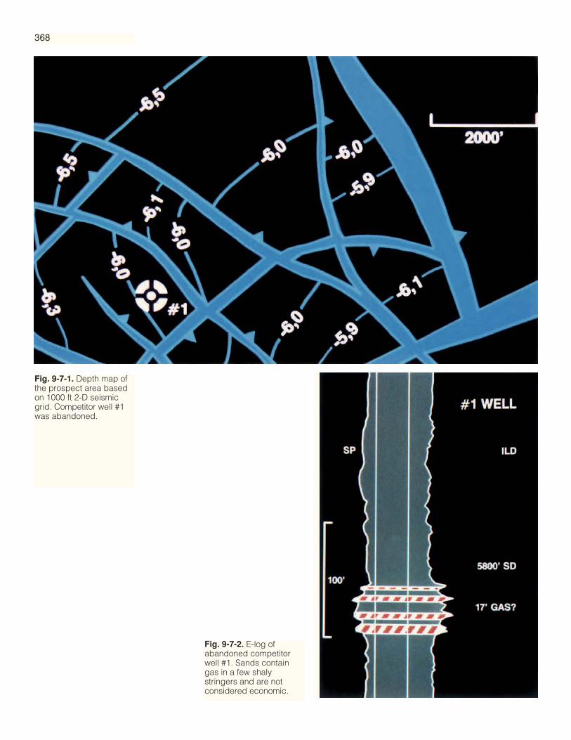
Fig. 9-7-1. Depth map ofthe prospect area basedon 1000 ft 2-D seismicgrid. Competitor well #1was abandoned.

Fig. 9-7-2. E-log ofabandoned competitorwell #1. Sands containgas in a few shalystringers and are notconsidered economic.

368

Fig. 9-7-3. Time map of the prospect area using 3-D sections and Seiscroptable. Note the significantchange in fault positions,orientations, and throws ascompared to 2-D map. Redline shows location of 3-Dline 118 (Figure 9-7-4).

369

Fig. 9-7-4. 3-D seismic line 118, east-west through the#1 well. Data are zero phase with trough = negativeacoustic impedance contrast. The bright spot can bedrilled 1000 ft west of the faulted #1 well.

Fig. 9-7-5. Color displayof line 118. Troughs areincreasing amplitudewhite-yellow-red; peaks,black-green-blue. Notethe detail not seen inclipped black-and-whitedata of Figure 9-7-4.Proposed #2 well is in aslightly weaker amplitudezone of the anomaly. Thismay not be an optimumdrilling location.

Fig. 9-7-6. Cube view of3-D data. Front face isline 118.

370

Fig. 9-7-7. Time structure map of top of bright spot based oninteractive analysis, picking maximum amplitude. Color bandsrepresent approximately 50-ft contours. Lines 118 and 123 arereferenced (Figures 9-7-5 and 9-7-8). Structural breaks in the

prospect map may be stratigraphic changes instead of faults.Subtle changes in the contours of up to 50 ft may be a responseto differential compaction (see also Figure 9-7-12).

371

Fig. 9-7-8. Line 123 suggests overlapping sand bodies on a common water contact.

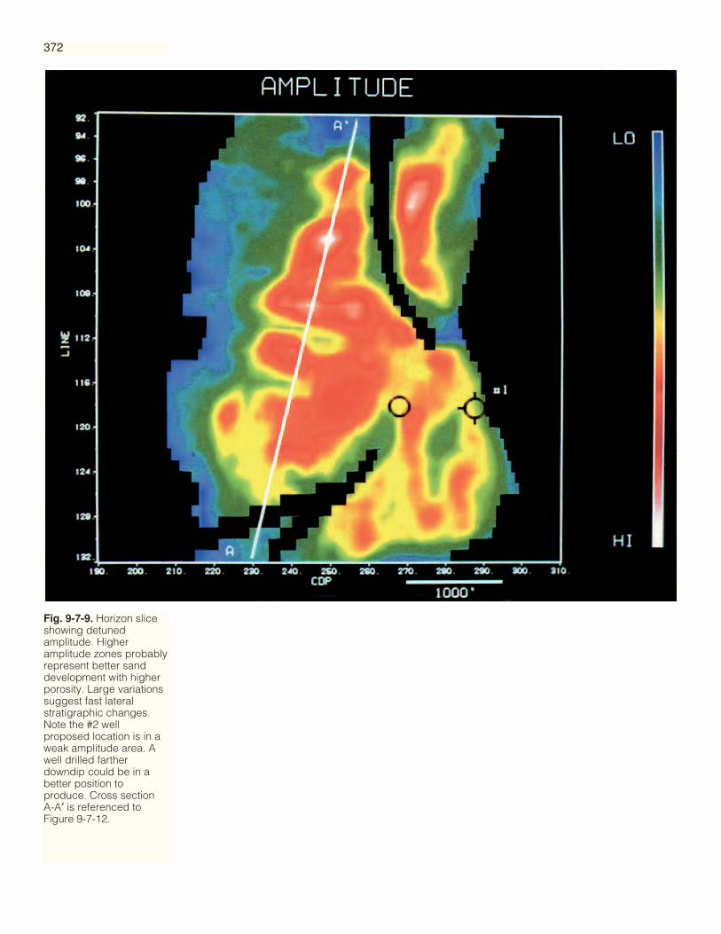
Fig. 9-7-9. Horizon sliceshowing detunedamplitude. Higheramplitude zones probablyrepresent better sanddevelopment with higherporosity. Large variationssuggest fast lateralstratigraphic changes.Note the #2 wellproposed location is in aweak amplitude area. Awell drilled fartherdowndip could be in abetter position toproduce. Cross section A-A′ is referenced toFigure 9-7-12.

372

373

Fig. 9-7-10. Net pay mapbased on seismic data.Note the #2 well wasdrilled downdip of theoriginal proposal. Aprediction of 58 ft of netpay was confirmed in the#2 well (Figure 9-7-11),which drilled 60 ft of gas.

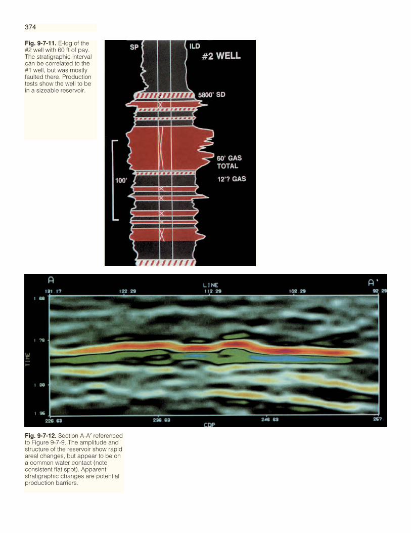
Fig. 9-7-11. E-log of the#2 well with 60 ft of pay.The stratigraphic intervalcan be correlated to the#1 well, but was mostlyfaulted there. Productiontests show the well to bein a sizeable reservoir.

Fig. 9-7-12. Section A-A′ referencedto Figure 9-7-9. The amplitude andstructure of the reservoir show rapidareal changes, but appear to be ona common water contact (noteconsistent flat spot). Apparentstratigraphic changes are potentialproduction barriers.

374

Case History 8

A 3-D Reflection Seismic Survey Over the Dollarhide Field,Andrews County, Texas

Michael T. Reblin, Gregory G. Chapel, Unocal North American Oil & Gas Division; Steven L.Roche, Chuck Keller, Halliburton Geophysical Services

Because onshore 3-D surveys can be expensive, the results may not be considered cost-effective. This case history presents an onshore 3-D survey that was cost-effective and thatshows the power of 3-D seismic versus well control and 2-D data.

Discovered in 1945, the Dollarhide field is a large faulted anticline in Andrews County whichis located on the Central Basin Platform of west Texas. Production in this field is from thePermian Clearfork, Devonian Thirty-one, Silurian Wristen, and Ordovician Ellenburger formations.(The commonly used names for the reservoirs are in italics.) Well spacing is approximately 40acres (16 ha) and the Devonian formation is currently undergoing CO2 flooding.

In August and September 1988, a 3-D survey was acquired over a 24 mi2 (62 km2) areacovering the Dollarhide field. The survey’s primary purpose was to accurately image thelocation of faulting within and bounding the Devonian. This would aid in planning the CO2flood and possibly locate previously untested fault blocks.

Geophysicists from Unocal and Halliburton Geophysical Services (HGS) worked together todesign the 3-D survey. Information (including depth of the main objective, velocity, maximumdip desired to be recorded, and reflection data quality) was compiled from previous 2-Dseismic data and geologic data from well logs. Migration aperture, Vibroseis sweep bandwidth,source and receiver arrays, CMP fold, and offset geometry were all modeled and examined foroptimum recording parameters. We determined that a subsurface bin size of 110 ft inline × 110ft crossline would adequately sample the subsurface for processing through 3-D migration.

The high cost of land 3-D seismic surveys has been a deterrent to their use in bothexploration and production geophysics. HGS suggested two innovations to reduce costs:

• Reduce the amount of data collected and replace it with trace interpolation prior to 3-Dmigration. Well control in the area reveals the general dip of the target horizon. Because thedip in the north-south direction is less steep than in the east-west direction, we could reducethe sampling in the former. We were able to use a subsurface sample interval of 110 ft (34 m)in the east-west (inline) direction and 330 ft in the north-south (crossline) direction, thusreducing by 66% the amount of data to be acquired. This also generated a further cost reliefbecause the lessened number of receiver and vibrator lines meant fewer surface accesspermits to be obtained. And, economies were realized also in data processing because thenumber of records that had to go through CMP stack was reduced by 66%.

• Use two vibrators simultaneously to sweep two separate lines. This technique improvedthe productivity of the recording crews by approximately 70%. The separation of the twosource signals is accomplished by upsweep-downsweep and phase rotation summing. Sourceseparation is performed in the field during the correlation and sum processes. The isolation ofthe two sources using this method is on the order of 40 dB.

The data were acquired using a 384-channel DFS VII recording system deployed as afour-line swath. The receiver lines were spaced 1320 ft (400 m) apart with two source linesper swath (Figure 9-8-1). Each swath generated eight subsurface profiles, separated by 330ft. After each swath, the spread was moved 2640 ft or 800 m (two cable lines) in thecrossline direction. This geometry results in the subsurface swaths being adjacent asopposed to overlapping. This can be described also as “one fold crossline.” With 12 swathsbeing recorded, the subsurface area is sampled 110 ft in the line and 330 ft in the crosslinedirections. The source interval averaged 440 ft (130 m). The resulting effective fold is 18-24when source-to-receiver offsets are considered relative to the depth of interest.

Data processing techniques included: geometry description; field record quality control;surface-consistent deconvolution; preliminary stack; velocity analysis; residual static

Introduction andSurvey Planning

Data Collectionand Processing

375

estimation; 3-D f-k DMO; stack; trace interpolation; and 3-D migration.At several steps during the processing of this survey, different parameters were tested

and reviewed — including the deconvolution method, benefit of DMO, migration velocityanalysis, and poststack migration algorithm. A benefit was realized by including DMO inthe processing sequence in that the diffracted image of the subsurface was improved. Thisenabled the trace interpolation algorithm to perform better in the conversion of 110 ft × 330ft subsurface bins to 110 ft × 110 ft bins. After 3-D migration, the data volume was moved toa workstation for interactive interpretation.

The results of this 3-D survey are impressive. Figure 9-8-2 shows the structure map of theDevonian at Dollarhide field as determined by the 40-acre-spaced well control. This map hasgone through many evolutions in the 46 years since the field was discovered. Notice that thecontours are relatively smooth, the anticline is cut by four simple cross-faults and bounded onthe east by a fault.

The structure map from the 3-D seismic survey (Figure 9-8-3) is more complex. Thecontouring is more detailed and the cross-faults are not simple. The structure map shows thedetail of the Devonian that the 3-D seismic has allowed us to see. This shouldn’t be a surpriseas our seismic data points are equivalent to a spacing of approximately four wells per acre.Considering that a seismic trace is an approximation to a synthetic seismogram from a soniclog, we indeed have a very powerful means of detail mapping subsurface structure.

There are two principal ways to look at the 3-D seismic data volume. One is theconventional seismic line display (Figure 9-8-4). On the crest of the structure, the top of theClearfork Formation is the strong event at approximately 780 ms. The Devonian, atapproximately 1000 ms on the upthrown block and 1350 ms on the downthrown block, iscolored purple. The top of the Ellenburger is a high-amplitude event at approximately 1250ms. At about 960 ms, an unconformity can be seen that helps highlight one of the moreremarkable features of the data — a fault zone showing over 2000 ft (610 m) of displacementon the Devonian marker. The imaging of this fault zone demonstrates one of theshortcomings of some 3-D surveys. Due to economics, lines may not be long enough toproperly image all the features (such as large faults or extremely steep dip) within the surveylimits. This survey was designed to image the upthrown block so that the incomplete imageeast of the major fault was as expected.

The other view of the 3-D data volume, and one not available with 2-D data, is the timeslice. This view allows the interpreter to see subtle features which may not be apparent or asreadily interpretable on conventional seismic sections. A time slice (Figure 9-8-5) through the3-D data volume at 1008 ms (about 4600 ft subsea or 7800 ft below surface) demonstrates this.The cross-faults are seen as northeast-southwest lineations. The previously undetected

Interpretation andResults

Fig. 9-8-1. Swath designof the 3-D dual sourcesurvey.

376

Fig

. 9-8

-2.S

imp

lifie

d D

evon

ian

stru

ctur

e m

ap fr

om 4

0-ac

re (

16-h

a) w

ell c

ontr

ol. T

he u

nit o

utlin

e is

red

.F

ig. 9

-8-3

.Sim

plif

ied

Dev

onia

n st

ruct

ure

map

from

3-D

seis

mic

inte

rpre

tatio

n.

377

Fig

. 9-8

-4.E

ast-

wes

t sei

smic

line

110

. Dev

onia

n ho

rizon

is a

nnot

ated

inp

urp

le; t

he in

terp

rete

d fa

ults

are

yel

low

.

378

379

Fig

. 9-8

-5.T

ime

slic

e at

100

8 m

s (a

bou

t 460

0 ft

[140

0 m

] su

bse

a or

780

0 ft

[238

0 m

] b

elow

sur

face

).D

evon

ian

horiz

on is

ann

otat

ed in

pur

ple

; the

inte

rpre

ted

faul

ts a

re y

ello

w.

380

Fig

. 9-8

-6.N

orth

east

per

spec

tive

view

of t

he D

evon

ian

time

stru

ctur

e m

ap.

The

colo

r ch

ang

e fr

om r

ed to

gre

en is

at t

he s

ame

time

as th

e tim

e sl

ice

inFi

gur

e 9-

8-5.

Not

e th

e cr

oss-

faul

t def

initi

on.

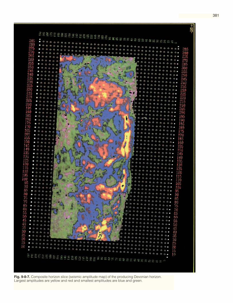
381

Fig. 9-8-7. Composite horizon slice (seismic amplitude map) of the producing Devonian horizon.Largest amplitudes are yellow and red and smallest amplitudes are blue and green.

grabens not seen on Figure 9-8-2 are seen as easterly pullouts on the time-sliced peaks (blue) andtroughs (red) in the areas of the cross-faulting. Mapping of the data is now possible in both thevertical and horizontal sense. Both offer unique perspectives of the data volume.

Because the 3-D survey gives an evenly sampled volume of data, another display of the datais possible after a horizon is interpreted. In Figure 9-8-6, a perspective view of the Devonianhorizon time map as viewed from the southwest is presented. It shows the northerly plunge ofthe anticline, which isn’t readily apparent on the Devonian horizon structure map (Figure 9-8-3).The cross-faults, with their associated grabens, are quite distinct and give a real feel for therelative throw of faults. This display has helped the geologists and engineers develop a betterunderstanding of the field shape and how the faults impact the ongoing CO2 flood project.

Having the 3-D data volume loaded on an interactive workstation allowed the interpreters togenerate various attribute displays that took us beyond the traditional time interpretation. Usingthe seismic peak and trough associated with the producing Devonian horizon, a compositehorizon slice (amplitude map) was made (Figure 9-8-7). The hot colors, yellow and red,represent larger amplitudes and, in most cases, correspond with the better wells in the field. Thecool colors, blue and green, represent lower seismic trace amplitudes along the producingDevonian. The amplitudes are interpreted to be related to the thickness of the producing zone —high amplitudes to a thick zone, low amplitudes to a thin zone. The possible exception is thelinear pattern next to the north-south bounding fault where we believe the larger amplitudes arepossibly related to poorly imaged steep dips. The major cross-faults are seen as northeast-southwest lineations, which divide the structure into four major fault blocks. The CO2 flood isexpected to have better results in the northern block which is denoted by the higher amplitudes.The flood was initiated in the northern block last year. The next block south has had the poorestflood results to date which seem related to the dominance of the lower amplitudes on thecomposite amplitude map. The third fault block was the first one flooded and has the bestresults to date, as could be predicted from the abundance of high amplitudes. The smallest faultblock, located to the southeast, is faulted below the producing limits of the field to the north.However, a well drilled to the productive Devonian horizon in 1948 recently has been reenteredand reevaluated, and could open up an extension to the field. The higher amplitudes indicate itcould be a very productive block with good CO2 flood potential.

Earlier in this case history, we alluded to the cost-effectiveness of this 3-D survey. One of thefeatures that helped us sell the concept to management was the comparison of the cost to shootthis 3-D survey to a 1/2 mi grid of 2-D data and the dryhole cost of a Devonian test. The 2-Dsurvey cost (including acquisition, surface permits, and processing) was estimated at $750,000for 150 line-mi. The dryhole cost of a Devonian test is approximately $300,000. To date, twoDevonian locations have not been drilled as the 3-D results indicated they were uneconomic.Shooting conventional swath 3-D to record 110 ft × 110 ft bins was estimated at about $1,300,000(generating 1140 mi (1820 km) of 3-D data over the 24 mi2). Using the 3-1 interpolation techniqueand simultaneous source recording, the survey actually cost $400,000. This cost is approximatelyhalf that for a 2-D survey, a third of a conventional 3-D survey, and only slightly more than a dryhole. The after-tax profit of a primary Devonian development well in the Dollarhide field isabout $1,000,000. By adding one well to the field, we easily recover the cost of the survey plusgive the geologists and engineers a more detailed look at a reservoir that is still being developedduring the tertiary recovery stage.

The results to date are multifold. The cross-faulting of the Devonian producing horizon ismuch more extensive than previously mapped. This knowledge has influenced the location ofseveral wells for the CO2 flood and the engineers continue to use the results for future programs.Some of the newly discovered faults have generated fault traps within the field that have notbeen drilled and are now being evaluated to determine their potential. Evidence suggests thatthe fault block to the southeast may be productive, although it was drilled and abandoned over40 years ago. Lastly, preliminary studies of the Clearfork Formation indicate the 3-D data willhelp in the development of the plan for the secondary recovery from that producing unit.

Land 3-D surveys can be economical and may produce results well beyond the initial goals.The two acquisition techniques discussed here are just two examples of how to shoot cost-effective land 3-D surveys. The 3-D seismic is a necessary tool to use in developing newdiscoveries and extending the life of old fields.

Conclusions

382

383

Case History 9

Shallow 3-D Seismic and a 3-D Borehole Profileat Ekofisk Field

John A. Dangerfield, Phillips Petroleum Company Norway

Ekofisk field in the Norwegian North Sea was discovered in 1969 but after more than 20years of production much remains to be understood (Sulak, 1990). This case historydescribes some of the 3-D seismic work carried out at Ekofisk field by the Phillips Licence018 Group of Companies: a short offset 3-D to image the very shallow layers, a normalsurface seismic 3-D especially processed for shallow data, and a 3-D borehole profile, shotto image the crest of the field beneath a gas cloud.

Figure 1 shows the areas covered by the various 3-D surveys. It also shows the reservoirarea that is obscured from normal seismic view by gas in the overlying sediments.

This survey was acquired in 1987 to delineate faults close to the Ekofisk Complex thatmight be reactivated by the (now) 5 m subsidence of the field (Wiborg and Jewhurst, 1986).The 4 × 2 km survey was collected with flip-flop acquisition, using single water guns as thesources, and recording 1.5 s of data. The twin hydrophone cables each contained 48 five mgroups. Reflection lines were 10 m apart. The processing was standard except for theextremely careful checking of recording geometry and effective time zero. One velocityfunction was used for the entire survey. A complete description is presented byDangerfield (1991).

The acquisition in 1989 was aimed at all possible levels from sea bottom to 7 s. The 9 × 17km area was shot using flip-flop, twin sources of 3680 in.3 air guns, and twin hydrophonecables, collecting reflection lines that were 25 m apart.

The data from the uppermost 2 s were processed separately in order to obtain the highestpossible resolution. They were processed with particular care in muting and velocityanalysis. Surprisingly, one velocity function was optimal for almost the complete area.

Imaging the crestal area below the gas never has been found possible with normal seismicmethods but borehole profiles generally have worked extremely well by undershooting thegas. The borehole profiles, however, have revealed many faults that can be linked in manydifferent patterns. The advantages of 3-D data sets for fault interpretation are so strong thatwe took the first opportunity to acquire a 3-D borehole profile in the gas-obscured area.

In July 1989, a series of 41 walkaway lines was shot into an eight-geophone array in thedeviated well 2/4 K17. Each single walkaway line thus recorded a swath of eight roughlyparallel reflection lines. The geophones in the array each were separated by 15 m. The holedeviation was about 45˚ so the geophone array spanned about 80 m horizontally. The 41walkaway lines were shot in a regular grid (Figure 9-9-2) with the geophone array pulledup the hole such that each walkaway line passed over the middle of the geophone array.The walkaway lines were 5 km long and perpendicular to the well. Successive lines were40 m apart. The acquisition area was limited by the presence of the Ekofisk Complex.

The acquisition resulted in a total of 328 reflection lines. Each line was processed separatelyto the velocity filter stage using standard walkaway techniques; then a one-pass migration ofthe whole data set was run, accomplishing both NMO and 3-D migration. Unfortunately, thedeepest 15 levels were so severely distorted by the gas that it was not useful to migrate thesedata. The input to the migration was restricted to data from geophones 3 to 6 in each array,overlapping geophones not being used. Crossline migration was performed using a slidingwindow of five geophone levels. The results were output as a regular 10 × 10 m grid.

The excellent resolution of the data, from the sea bottom at 100 ms down to 1 km depth,showed that there were no faults with throws of more than 2 m in the region examined.

Acquisition andProcessing of theShort Offset 3-D

Acquisition andProcessing of theNormal SurfaceSeismic

Acquisition andProcessing of the 3-D BoreholeProfile

Interpretation of theShort Offset Data

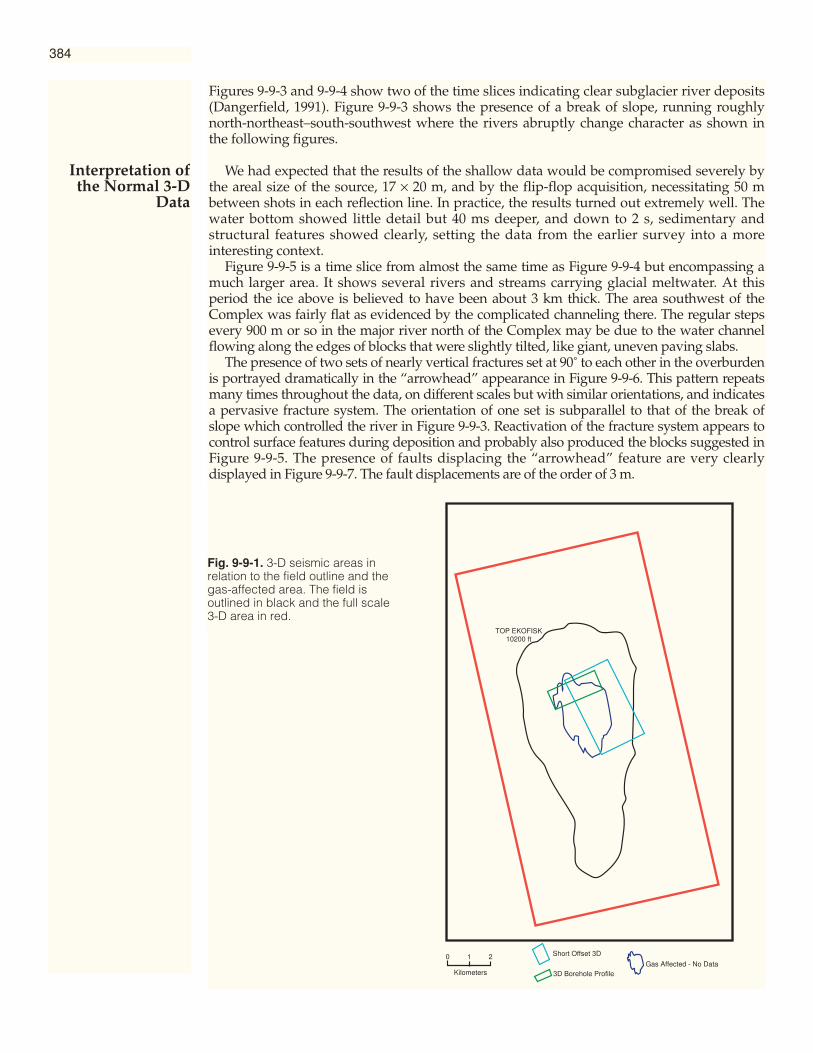
384

Figures 9-9-3 and 9-9-4 show two of the time slices indicating clear subglacier river deposits(Dangerfield, 1991). Figure 9-9-3 shows the presence of a break of slope, running roughlynorth-northeast–south-southwest where the rivers abruptly change character as shown inthe following figures.

We had expected that the results of the shallow data would be compromised severely bythe areal size of the source, 17 × 20 m, and by the flip-flop acquisition, necessitating 50 mbetween shots in each reflection line. In practice, the results turned out extremely well. Thewater bottom showed little detail but 40 ms deeper, and down to 2 s, sedimentary andstructural features showed clearly, setting the data from the earlier survey into a moreinteresting context.

Figure 9-9-5 is a time slice from almost the same time as Figure 9-9-4 but encompassing amuch larger area. It shows several rivers and streams carrying glacial meltwater. At thisperiod the ice above is believed to have been about 3 km thick. The area southwest of theComplex was fairly flat as evidenced by the complicated channeling there. The regular stepsevery 900 m or so in the major river north of the Complex may be due to the water channelflowing along the edges of blocks that were slightly tilted, like giant, uneven paving slabs.

The presence of two sets of nearly vertical fractures set at 90˚ to each other in the overburdenis portrayed dramatically in the “arrowhead” appearance in Figure 9-9-6. This pattern repeatsmany times throughout the data, on different scales but with similar orientations, and indicatesa pervasive fracture system. The orientation of one set is subparallel to that of the break ofslope which controlled the river in Figure 9-9-3. Reactivation of the fracture system appears tocontrol surface features during deposition and probably also produced the blocks suggested inFigure 9-9-5. The presence of faults displacing the “arrowhead” feature are very clearlydisplayed in Figure 9-9-7. The fault displacements are of the order of 3 m.

Interpretation ofthe Normal 3-D

Data

TOP EKOFISK10200 ft

0 1 2

Kilometers

Short Offset 3D

3D Borehole ProfileGas Affected - No Data

Fig. 9-9-1. 3-D seismic areas inrelation to the field outline and thegas-affected area. The field isoutlined in black and the full scale3-D area in red.

385

Although only a brief selection of time slices from the shallower layers have been shown,the complete 3-D data sets form continuous series, with slight but distinct differences insuccessive slices, so that the evolution of the sedimentary features can be followed on ameter by meter basis.

The resulting borehole profile in the northern half of the data set showed a clear image inan area where our 3-D surface seismic failed completely. Figures 9-9-8, 9-9-9, and 9-9-10locate and compare line 40 from the 3-D borehole profile with a 3-D surface seismic linefrom the same place. Figure 9-9-11 shows line 16 (east-west) and crossline 150 (north-south)with the top Ekofisk Formation interpreted. The data showed the presence of many faultstoo small to map but with similar orientations to those of the overburden fracture system. Italso showed the continuation of a crestal graben originally found in the gas-affected area bywalkaway profiling (Christie and Dangerfield, 1987) and subsequently penetrated bydrilling. Figure 9-9-12 shows a time slice through the reservoir with the top Ekofisk markedin green. The graben clearly displaces the Ekofisk horizon.

1) The normal 3-D shallow data set showed the fracture system that pervades the Tertiaryand controlled some surface features during deposition.

2) High quality data close to the water bottom is readily available in the shallow sectionin normal 3-D data sets. This suggests that an important part of the work currently carriedout by site survey vessels is accomplished in the course of a normal 3-D survey.

Interpretation ofthe 3-D BoreholeProfile

Conclusions

Fig. 9-9-2. 3-D boreholeprofile acquisition linessuperimposed on the1989 top reservoir depthmap.

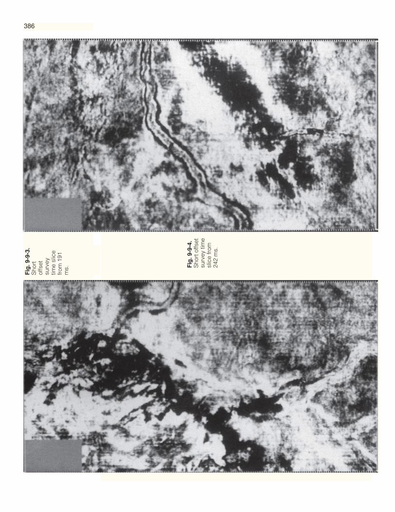
386F

ig. 9

-9-3

.S

hort

offs

etsu

rvey

time

slic

efr

om 1

91m

s. Fig

. 9-9

-4.

Sho

rt o

ffset

surv

ey ti

me

slic

e fr

om24

2 m

s.

387

3) The 3-D borehole profile showed the extent of the crestal grabens inside an areaopaque to normal seismic methods.

4) 3-D borehole profiles should be considered as a working alternative to 2-D boreholeprofiles since the extra rig time and cost are surprisingly small and the benefits of 3-D aresubstantial. The method should be particularly suitable for time-lapse reservoir monitoring.

The statements in this case history reflect those of the author and not necessarily those ofany of the Phillips Licence 018 Group of Companies. The author thanks the above Group forpermission to publish the data.

Brewster, J., J. Dangerfield, and H. Farrell, 1986, The geology and geophysics of the Ekofiskfield waterflood: J. Marine and Petroleum Geology, v. 3, p. 139-170.

Christie, P. A. F., and J. A. Dangerfield, 1987, Borehole seismic profiles in the Ekofisk field:Geophysics, v. 152, p. 1328-1345.

Dangerfield, J. A., in press, Ekofisk field — Subsidence fault analysis using 3-D seismic, inReservoir Geophysics, R. E. Sheriff, A. R. Brown, D. Johnston, J. Justice, and R. Hardage:SEG/SPE/AAPG, in press.

Sulak, R. M., 1990, Ekofisk field — the first twenty years: SPE Annual Conference, NewOrleans, September 1990.

Wiborg, R., and J. Jewhurst, 1986, Ekofisk subsidence detailed and solutions assessed: Oiland Gas Journal, v. 84, no. 7, p. 47-55.

Fig. 9-9-5. Full-scalesurvey time slice from244 ms.

References

388

Fig. 9-9-6. Full-scalesurvey time slicefrom 512 ms.

Fig. 9-9-7. Full-scalesurvey time slicefrom 566 ms.

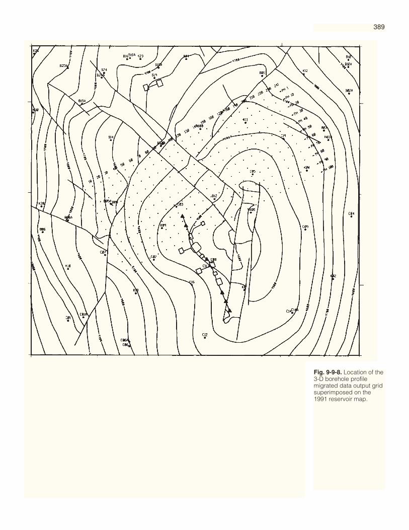
389

Fig. 9-9-8. Location of the3-D borehole profilemigrated data output gridsuperimposed on the1991 reservoir map.

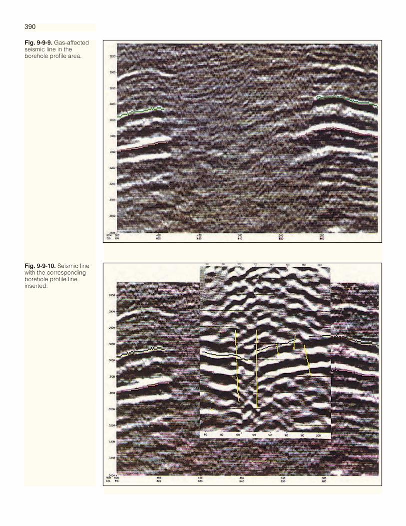
390

Fig. 9-9-10. Seismic linewith the correspondingborehole profile lineinserted.

Fig. 9-9-9. Gas-affectedseismic line in theborehole profile area.

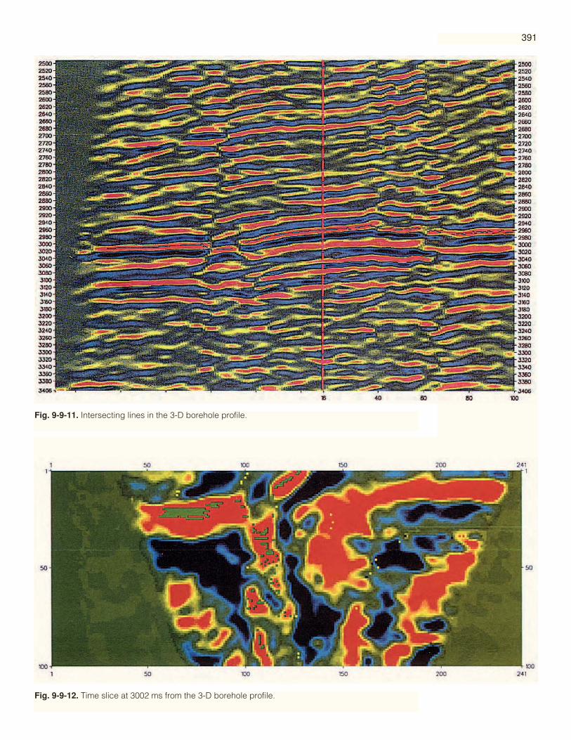
391

Fig. 9-9-11. Intersecting lines in the 3-D borehole profile.

Fig. 9-9-12. Time slice at 3002 ms from the 3-D borehole profile.

392

Case History 10

Extending Field Life in Offshore Gulf of Mexico Using 3-DSeismic Survey

Thomas P. Bulling, Rebecca S. Olsen, ARCO Oil and Gas Company

The High Island 24L field (ARCO), located in the Texas state waters of the Gulf of Mexico, wasdiscovered in 1967. It had produced 320 billion cubic feet (bcf) of gas and 3.0 million bbl of oil by1986. An engineering field study completed in 1986 projected the field declining to the point ofunprofitability within three years. The study found the reservoir maps had three basic problems:volumetric reserve calculations did not equal reserves produced; hydrocarbon-water contacts wereinconsistent between wells thought to be in communication; and maps did not define extensionopportunities. Attempts to remap the field with the existing 2-D seismic data base and well logsproved unsuccessful.

In 1986, ARCO acquired a 3-D seismic survey and, in 1987, remapped the field starting with thekey producing horizons. Integration of detailed well log correlations with the dense grid of 3-Dseismic allowed construction of accurate reservoir maps. These new maps helped solve theengineering problems by more accurately defining the configuration of the reservoirs, closelymatching volumetrics and fluid contacts as well as defining new extension opportunities. The 3-Dseismic survey and its products, along with engineering modifications and operations costcontainment, resulted in the extension of the field’s economic life by at least eight years. As morewells are drilled and new information integrated, additional reserves are found.

Many fields in the Gulf of Mexico discovered with the seismic data available in the 1960s and early1970s are facing declining production and reaching the end of their economic life. After discovery andinitial development drilling, many of these fields were simply put on production and maintained.High Island 24L field is an example of such a field; only two wells were drilled between 1972 (the endof development drilling) and 1986. 3-D seismic is often needed to extend the life of these mature oiland gas fields. High Island 24L field is an excellent example of using 3-D seismic for this extension.

The High Island 24L field is ten miles offshore in the Texas state waters of the Gulf of Mexico.Discovered by ARCO in 1967, the field has produced 320 bcf of gas and 3 million bbl of oil from 30lower Miocene sands ranging from the normally pressured CM-12 (Robulus 43) sand to thegeopressured “KI” sand (Figure 9-10-1). The field produces from anticlinal and fault traps bothupthrown and downthrown to a lower Miocene growth fault system (Figure 9-10-2).

In 1986, a reservoir engineering study indicated the field would become unprofitable in twoyears (Figure 9-10-3, green line). The study also identified some key problems with the reservoirmaps including: reservoir volumetrics did not equal production (i.e., several fault blocks producedmore than maps indicated); structure maps and fluid level contacts were inconsistent (wells withinthe same fault block had different gas/water contacts); engineers could not reasonably forecastultimate reserves; and maps did not define extension opportunities.

Prompted by the engineering study, ARCO attempted to remap the field to better evaluate itspotential. The endeavor represented the first integration of geology, geophysics, and engineeringdata since development drilling ended in 1972. However, the available 2-D seismic data wereinadequate and could not resolve the mapping problems. The question arose whether toabandon/sell the field or acquire more high-quality seismic data. Because the 2-D mapping provedunsuccessful, we could not place a reliable value on the property on which to base abandonment orselling criteria. Geoscientists felt chances were good that untested reservoirs would be found ifaccurate maps could be generated. Therefore, ARCO decided to obtain better seismic data todetermine the value and potential of the field.

After considering several options, we decided not to acquire more 2-D data since 14 vintagesalready existed (shot between 1967 and 1985). A dense, consistent 3-D survey would greatly benefitthe project in five ways: improved mapping of subtle structures; identification and evaluation ofamplitude anomalies related to hydrocarbon bearing sands; resolution of deep, complicatedstructures; integration with data from numerous wells; and the ability to manipulate the seismic

Introduction

Background andGeology

393

data in a variety of ways using a 3-D interactive workstation. Cost of the survey was less per milethan 2-D and less than the cost of a shallow well in this field. Geoscientists began mapping the fieldin June 1987 using the 3-D seismic data. Initial work focused on the most prolific reservoir sands.

Significant mapping changes appeared between old 2-D and new 3-D maps. This sectionillustrates three examples of these changes in the “HC,” “KC,” and CM-12 horizon interpretations.

The “HC” (Siphonina davisi in age) sand at about 8000 ft (2400 m) is the most prolific reservoir.The 3-D seismic data clearly identifies subtle structures not seen on 2-D seismic lines and not foundon the old maps (Figures 9-10-4a and 9-10-4b). Three wells, B-2, 9, and B-4, drilled on subtlestructural highs, found the “HC” sand productive. Figure 9-10-5 is a seismic example of a subtle“HC” high tested by the successful (post-3-D) #9 well. This example shows how 3-D helped toidentify untested subtle structures and allowed us to generate seismic traverses to see relationshipsbetween drilled and proposed wells.

The second example shows mapping improvements in one of the deepest producing horizons,the “KC” (Lower Planulina in age), at about 11,000 ft. Figures 9-10-6a and 9-10-6b illustrate thedrastic differences between the pre-3-D and the post-3-D maps. These maps are similar in area andorientation. Understanding fluid contacts and reservoir juxtaposition across faults always had beena problem in the Lower Planulina sands. The new, post-3-D map is based on new well loginterpretation integrated with the 3-D seismic. This recent interpretation explains areas wherevolumetrics and fluid contacts previously did not make sense.

Mapping success at “KC” is largely due to the improvement in deep seismic resolutionintegrated with a new well log interpretation. Figures 9-10-7a and 9-10-7b are portions of seismiclines from the 2-D and 3-D data sets. Improvement in deep resolution on 3-D line 112 (Figure 9-10-7b) is demonstrated by clearer fault trace delineation and reflection continuity.

The final example of mapping changes is from the shallowest producing horizon, CM-12(Robulus 43 in age), at about 5500 ft (1680 m). Old 2-D mapping (Figure 9-10-8a) is different from thenewer post-3-D map (Figure 9-10-8b). Significant to the post-3-D map is a four-way dip structure onblock 90S not adequately tested by the two wells on this block. Prior to interpreting the 3-D data,we did not recognize the 90S structure and the amplitude anomaly that conforms to it (Figure 9-10-9). This anomaly is very similar to a CM-12 anomaly known to produce in wells #4 and #5. Anarbitrary line known as seismic traverse 11 (Figure 9-10-10) shows the relationship between theprospective 90S block amplitude and that of the producing #4 and #5 wells. Drilled in early 1988,the ARCO 90S #1 well found hydrocarbon-bearing sands causing the CM-12 amplitude anomaly.Also, CM-12 came in very close to target depth and expected reserve size. This example illustratesthe ability of the interpreter to identify amplitude anomalies in a small area. Utilizing the 3-Dworkstation, we can relate the untested anomalies to similar productive anomalies in the field,resulting in reduced risk and better reservoir delineation.

The post-3-D maps resulted in drilling and completing eight wells to date that will recover 40 bcfequivalent (net to ARCO). The 3-D seismic survey was an excellent investment, costing less than ashallow well in the field. The new wells, based on 3-D mapping, resulted in a reversal of the field’sdeclining Before Federal Income Tax cash flow curve (Figure 9-10-3, red line). Other wells currentlyare under consideration. In total, the post-3-D maps identified 50 bcf equivalent of potentialreserves (40 bcf from new wells and 10 bcf from existing wells and recompletions).

The 3-D seismic survey aided our interpretation of the field by providing:• a continuous and dense grid of data across the field;• the capability to generate traverses at any orientation;• excellent detection of subtle structures;• horizon slices to help define accumulations on the basis of amplitude;• better deep resolution to help add extension opportunities.Overall, the use of 3-D seismic data allowed for a better understanding of the stratigraphic and

structural complexities of the High Island 24L field. In addition, post-3-D maps helped solve theengineering problems by more accurately defining the configuration of the reservoirs. Reservoirmaps now closely match volumetrics; fluid contacts within fault blocks are consistent; and we havea better definition of the extension opportunities available. The 3-D seismic survey and its products,along with engineering modifications and operations cost containment, resulted in the extension ofthe economic life of the field to at least 1996.

Results andExamples

Conclusions

394

Fig. 9-10-1. The type logfor the High Island 24Lfield illustrating the 30 paysands. The “HC” sand isthe most productivereservoir.

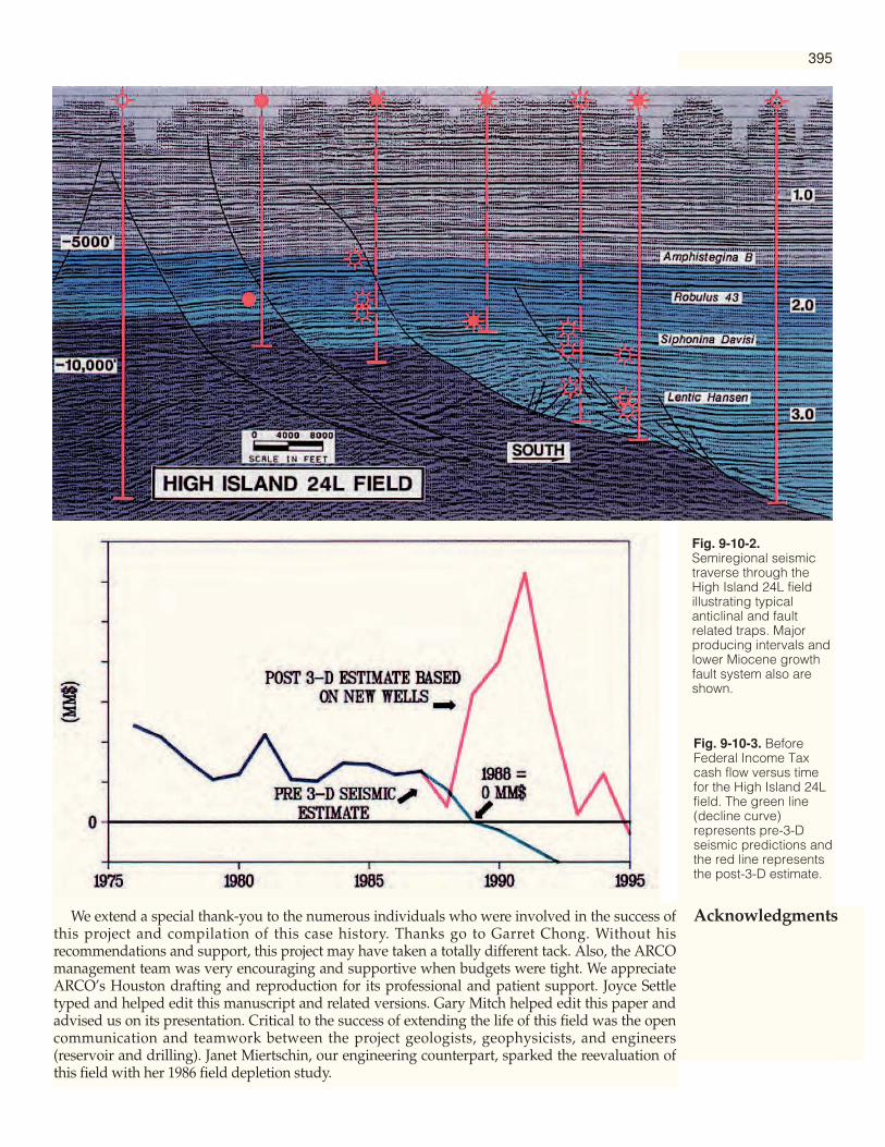
395

We extend a special thank-you to the numerous individuals who were involved in the success ofthis project and compilation of this case history. Thanks go to Garret Chong. Without hisrecommendations and support, this project may have taken a totally different tack. Also, the ARCOmanagement team was very encouraging and supportive when budgets were tight. We appreciateARCO’s Houston drafting and reproduction for its professional and patient support. Joyce Settletyped and helped edit this manuscript and related versions. Gary Mitch helped edit this paper andadvised us on its presentation. Critical to the success of extending the life of this field was the opencommunication and teamwork between the project geologists, geophysicists, and engineers(reservoir and drilling). Janet Miertschin, our engineering counterpart, sparked the reevaluation ofthis field with her 1986 field depletion study.

Acknowledgments

Fig. 9-10-2.Semiregional seismictraverse through theHigh Island 24L fieldillustrating typicalanticlinal and faultrelated traps. Majorproducing intervals andlower Miocene growthfault system also areshown.

Fig. 9-10-3. BeforeFederal Income Taxcash flow versus timefor the High Island 24Lfield. The green line(decline curve)represents pre-3-Dseismic predictions andthe red line representsthe post-3-D estimate.

396

Fig

. 9-1

0-4b

.Pos

t-3-

Dse

ism

ic “

HC

” sa

ndst

ruct

ure

map

. Not

e th

atth

e su

btle

hig

hs o

n w

hich

wel

ls 9

, B-2

, and

B-4

wer

e d

rille

d d

o no

t exi

ston

pre

-3-D

str

uctu

re m

ap(F

igur

e 9-

10-4

a).

Fig

. 9-1

0-4a

.Pre

-3-D

seis

mic

“H

C”

sand

stru

ctur

e m

ap.

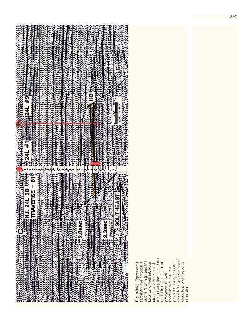
397

Fig

. 9-1

0-5.

Trav

erse

81

(arb

itrar

y lin

e) th

roug

h a

sub

tle “

HC

” hi

gh

and

the

loca

tion

of w

ell #

9. N

ote

stru

ctur

al e

leva

tion

and

trou

gh

amp

litud

e in

crea

seup

dip

from

24L

#1

to th

ep

rop

osed

#9

wel

llo

catio

n. W

ell 2

4L #

9p

rove

d to

be

succ

essf

ul,

clos

e to

targ

et d

epth

, and

clos

e to

pre

-dril

l res

erve

estim

ates

.

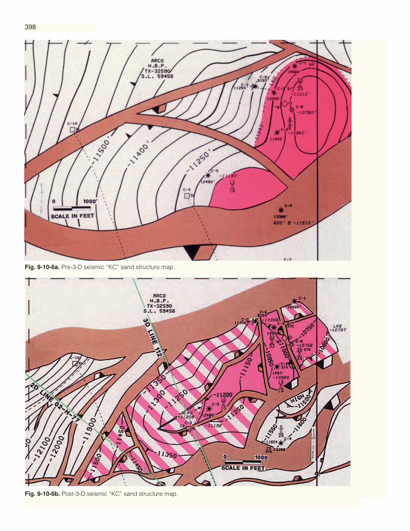
398

Fig. 9-10-6b. Post-3-D seismic “KC” sand structure map.

Fig. 9-10-6a. Pre-3-D seismic “KC” sand structure map.

399

Fig. 9-10-7b. 3-D seismic line 112. Location of this line is shownon Figure 9-10-6b. Areas highlighted on Figures 9-10-7a and bare comparable. Line 112 is superior in deep resolution.

Fig. 9-10-7a. 2-D seismic line 02-H-77. Location of this line is shown on Figure 9-10-6b.

400

Fig

ure

9-1

0-8b

.Pos

t-3-

D s

eism

ic C

M-1

2 st

ruct

ure

map

. Str

uctu

ral c

losu

re in

blo

ck 9

0S w

as n

ot te

sted

by

the

two

wel

ls in

this

blo

ck. A

n am

plit

ude

anom

aly

conf

orm

s to

this

str

uctu

re.

Fig

. 9-1

0-8a

.Pre

-3-D

sei

smic

CM

-12

stru

ctur

e m

ap. N

o st

ruct

ure

or a

mp

litud

ean

omal

y in

blo

ck 9

0S w

as n

oted

whe

n th

is m

ap w

as m

ade.

401

Fig. 9-10-9. CM-12 horizon slice (also termed amplitude map) illustrates strong trough amplitudes (pinks and reds)conforming to the 90S block structure (in the northwest corner of the figure). The 90S anomaly is stronger than the #4and #5 producing anomaly to the southeast.

402

Fig

. 9-1

0-10

.Sei

smic

trav

erse

11 (

arb

itrar

y lin

e) s

how

ing

the

CM

-12

trou

gh

amp

litud

ean

omal

ies

mar

ked

in y

ello

w fo

rth

e 90

S b

lock

and

for

the

pro

duc

tion

in w

ells

#4

and

#5.

Loca

tion

of th

e tr

aver

se is

show

n on

Fig

ures

9-1

0-8b

and

9-10

-9.

Case History 11

Modern Technology in an Old Area — Bay MarchandRevisited

W. L. Abriel, P. S. Neale, J. S. Tissue, R. M. Wright, Chevron USA, Inc.

Bay Marchand, a giant oil field in the Gulf of Mexico, is undergoing renewed drillingactivity as the result of a recently acquired 3-D seismic survey. This classic mature fieldseemingly had entered its last stages of production in the mid-1980s. However, anintegrated team effort by geologists, geophysicists, and engineers revitalized the area byinnovative use of the new 3-D data.

Figure 9-11-1 shows the relative location of Bay Marchand to the Louisiana coastline. Thefield is approximately 65-70 mi (105-110 km) south of New Orleans and in state coastalwaters. Water depths range from 10 to 50 ft (3 to 15 m). The field is situated across a hugesalt diapir and its geology is characterized by complex faulting and stratigraphy. The latteris due to regressive marine sequences; the former is caused by both salt movement andsediment loading.

The first well, which was dry, was drilled in 1930. It then took 19 years and 11 more dryholes before the first discovery was made in 1949. This says something about thepersistence of the early geologists and early management. There have been more than 800wells drilled in the field to date.

Bay Marchand officially became a giant in 1986 when its 500 millionth bbl of oil wasproduced. At that time, though, it did not appear that much more could be extracted. Dailyproduction had peaked at more than 75,000 bbl of oil/day in the late ’60s and early ’70s. Asteady decline occurred through the remainder of the ’70s and into the ’80s. This declinecontinued in spite of engineering waterflood efforts in the ’70s and acquisition of modern 2-D seismic data in the early ’80s. When production dipped to 18,000 bbl of oil/day in themid-1980s, a 3-D survey was contracted. The intent was to arrest further production declineand possibly to reverse the trend.

The decision to shoot the 3-D survey was based on three objectives:• Delineate new reservoirs and discover additional reserves that might be hidden in both

structural and stratigraphic traps.• Review the drilled areas and sort out the complex faulting and stratigraphy in order to

determine where additional wells would facilitate production of already proved reserves.• Assist in reservoir management via unification of the disciplines of geology,

geophysics, and engineering in an attempt to obtain better models for reservoir simulationand to optimize the location of water injection wells for EOR.

Figure 9-11-2 shows in red the fully migrated portion of the 3-D survey. The areal extentof this area is over 60 mi2 (150 km2). This survey, acquired in 1988, covers most of Chevron’sleased acreage (yellow line). It was recognized that a data set of exceptional quality wasrequired to achieve the survey’s objectives. To this end, the following four geophysicalrequirements were adopted:

• Cover all CDP bins.• Obtain maximum resolution, both horizontal and vertical, because both are necessary

to enable the isolation of many reflectors from the top and base of sand units and toevaluate stratigraphic changes.

• Obtain consistent offset and azimuth distribution.• Obtain the best geometry — meaning that extra care had to be taken in the navigation

quality control to ensure that data were obtained in the locations intended.Achieving these objectives would require the best possible field techniques because the

survey area contained many items that could significantly interfere with data acquisition. Inaddition to a water bottom that was nearly solid with pipelines and high voltage power

403

Background

Objectives

Acquisition

404

cables, there were 114 surface obstacles in the form of single- and multi-well drillingplatforms. This mandated that data be acquired via a state-of-the-art telemetry technique.

Western Geophysical’s Digiseis acquisition system was employed for this survey. In thissystem a hydrophone is placed on the ocean floor and connected to digital electronics thatare floating on the surface. All data are transmitted via antenna to the recording vessel.Since the hydrophones are not connected to each other by a long and cumbersome cable,this system makes it possible to position hydrophones in close proximity to the manysurface facilities. In fact, it was sometimes necessary and possible to put the systemsbeneath the platforms. On most occasions, however, it was possible to obtain data atdesignated surface points by switching shot and receiver locations and/or undershootingthe platform. The acquisition consisted of narrow swaths. The lines of receivers were laidout 880 ft (270 m) apart, and spaced at intervals of 220 ft (70 m) inline. Shots were takenevery 110 ft in four rows laid out 220 ft apart and parallel to the receiver lines. This created a3-D bin size of 55 ft × 110 ft (which was then interpolated to 55 ft × 55 ft for migration). Finalcoverage was 60-fold.

Due to careful acquisition techniques, the midpoint location plots differed from thoseencountered in a normal marine survey in two respects: (1) The bin size of 55 ft rather thanthe normal 82 ft was smaller, and (2) the midpoints were clustered in the center of the binsrather than scattered over the bin. It was believed these factors would significantly improvehorizontal resolution in the final data.

The fold of coverage charts confirmed the excellent quality and even distribution of thedata. There were no gaps due to the 114 surface structures, and no “striping” due to thehydrophones drifting to locations other than the desired sites. This is important because itincreases confidence in interpretation of amplitude variations as being the result ofsubsurface geologic or petrophysical changes.

To date, the 3-D survey has helped the structural interpretation significantly in two keyareas. First, the salt/sediment interface is better defined, and second, the complex faultgeometries are better resolved.

Figure 9-11-3 is a time slice at approximately 5000 ft (1500 m). The quality is good andsignal content strong. Most importantly, there is a clear definition of the salt/sediment

Fig. 9-11-1. Location ofthe Bay Marchand fieldoffshore Louisiana.

Structural Benefits

405

interface in the core of the structure. This definition is very important because largeamounts of hydrocarbons are trapped against this interface. Notice the irregular andunusual shape of this interface. Most geologists and management had anticipated an ovalcore shape and one that was much smoother. Certainly, the sharp corners of salt were notexpected.

Figure 9-11-4 is a vertical section across the Bay Marchand salt dome. Again, note thesharp definition of the salt/sediment interface. Several well-defined faults also are evident.These must be accurately mapped because large reserves are trapped against them. Note, inaddition, the sharp corners on the top of the salt. Some are undoubtedly enhanced by theacquisition and processing techniques employed.

Another perspective concerning the improvement in salt/sediment interface resolution isgiven in the next four figures. Figure 9-11-5 shows a top-salt structure map that wasprepared prior to the availability of 3-D seismic control. This map, therefore, was generatedusing subsurface control which was quite abundant in the area. Note that there are 23 wellpenetration points; that is generally sufficient control over such an area for adequate top saltmapping by geologists. However, note the shape of the 5000 ft contour and compare withFigure 9-11-6.

Figure 9-11-6 is a time slice at approximately 5000 ft over the same area as Figure 9-11-5.Note the well-defined salt mass and the strong salt/sediment interface reflection. The latterindicates a large salt embayment which is not seen from the well control. This is a criticalpiece of information because it implies a potential reservoir, as sands may be trapped upagainst salt in this embayment. A usertrack along A-A′ should evaluate that potential.

Figure 9-11-7 shows the A-A′ usertrack and the concept of the prospect. The area ofimmediate interest is in the center of the section at 1.5 s. Note the high amplitude reflectionsand the good salt/sediment interface. Previous mapping had brought the highest area of salt

Fig. 9-11-2. Migrated 3-Dsurvey outlinesuperimposed on thestructure of top salt.

406

Fig. 9-11-3. Time slice at1.5 s showing salt-sediment interface.

0 4000′ V.E. =2x

2000′

Fig. 9-11-4.Northeast-southwestseismic crosslinefrom the 3-D surveyshowing structuraldetail at the saltinterface.

407

N

1000′

Fig. 9-11-5. Top saltstructure generated from23 wells prior to the 3-Dsurvey.

Fig. 9-11-6. Timeslice at 1.5 s (detailof Figure 9-11-2)correspondingapproximately toFigure 9-11-5.

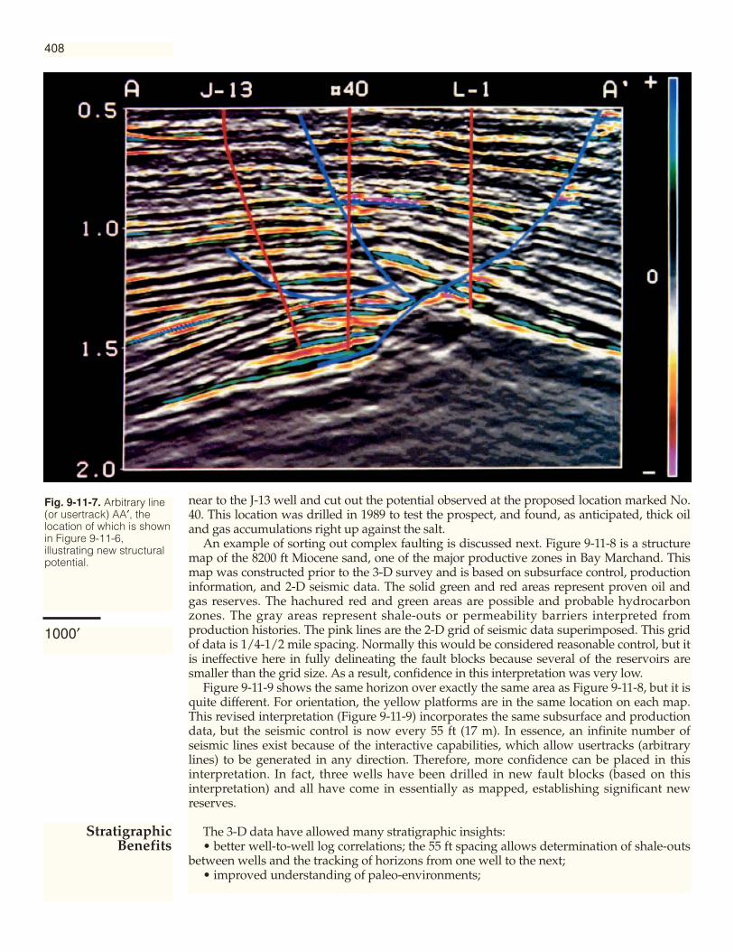
408

near to the J-13 well and cut out the potential observed at the proposed location marked No.40. This location was drilled in 1989 to test the prospect, and found, as anticipated, thick oiland gas accumulations right up against the salt.

An example of sorting out complex faulting is discussed next. Figure 9-11-8 is a structuremap of the 8200 ft Miocene sand, one of the major productive zones in Bay Marchand. Thismap was constructed prior to the 3-D survey and is based on subsurface control, productioninformation, and 2-D seismic data. The solid green and red areas represent proven oil andgas reserves. The hachured red and green areas are possible and probable hydrocarbonzones. The gray areas represent shale-outs or permeability barriers interpreted fromproduction histories. The pink lines are the 2-D grid of seismic data superimposed. This gridof data is 1/4-1/2 mile spacing. Normally this would be considered reasonable control, but itis ineffective here in fully delineating the fault blocks because several of the reservoirs aresmaller than the grid size. As a result, confidence in this interpretation was very low.

Figure 9-11-9 shows the same horizon over exactly the same area as Figure 9-11-8, but it isquite different. For orientation, the yellow platforms are in the same location on each map.This revised interpretation (Figure 9-11-9) incorporates the same subsurface and productiondata, but the seismic control is now every 55 ft (17 m). In essence, an infinite number ofseismic lines exist because of the interactive capabilities, which allow usertracks (arbitrarylines) to be generated in any direction. Therefore, more confidence can be placed in thisinterpretation. In fact, three wells have been drilled in new fault blocks (based on thisinterpretation) and all have come in essentially as mapped, establishing significant newreserves.

The 3-D data have allowed many stratigraphic insights:• better well-to-well log correlations; the 55 ft spacing allows determination of shale-outs

between wells and the tracking of horizons from one well to the next;• improved understanding of paleo-environments;

Fig. 9-11-7. Arbitrary line(or usertrack) AA′, thelocation of which is shownin Figure 9-11-6,illustrating new structuralpotential.

1000′

StratigraphicBenefits

409

Fig. 9-11-8.Structure mapof 8200 ft sandprior to the 3-Dsurvey. Provenoil and gas areshown ingreen and red.2-D seismiccontrol isshown in pinklines. Fortywellpenetrationscontrol thismap.

Fig. 9-11-9.Structure mapof 8200 ft sandafter evaluationof the 3-Dsurvey. Notethat no faultsare the sameas in Figure 9-11-8.

1000′

N

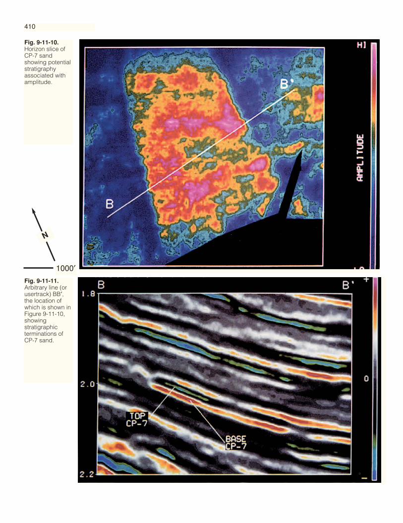
410

Fig. 9-11-10.Horizon slice ofCP-7 sandshowing potentialstratigraphyassociated withamplitude.

Fig. 9-11-11.Arbitrary line (orusertrack) BB′,the location ofwhich is shown inFigure 9-11-10,showingstratigraphicterminations ofCP-7 sand.

1000′

N

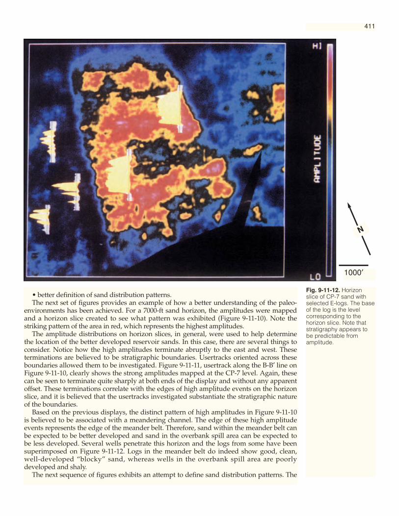
411

• better definition of sand distribution patterns.The next set of figures provides an example of how a better understanding of the paleo-

environments has been achieved. For a 7000-ft sand horizon, the amplitudes were mappedand a horizon slice created to see what pattern was exhibited (Figure 9-11-10). Note thestriking pattern of the area in red, which represents the highest amplitudes.

The amplitude distributions on horizon slices, in general, were used to help determinethe location of the better developed reservoir sands. In this case, there are several things toconsider. Notice how the high amplitudes terminate abruptly to the east and west. Theseterminations are believed to be stratigraphic boundaries. Usertracks oriented across theseboundaries allowed them to be investigated. Figure 9-11-11, usertrack along the B-B′ line onFigure 9-11-10, clearly shows the strong amplitudes mapped at the CP-7 level. Again, thesecan be seen to terminate quite sharply at both ends of the display and without any apparentoffset. These terminations correlate with the edges of high amplitude events on the horizonslice, and it is believed that the usertracks investigated substantiate the stratigraphic natureof the boundaries.

Based on the previous displays, the distinct pattern of high amplitudes in Figure 9-11-10is believed to be associated with a meandering channel. The edge of these high amplitudeevents represents the edge of the meander belt. Therefore, sand within the meander belt canbe expected to be better developed and sand in the overbank spill area can be expected tobe less developed. Several wells penetrate this horizon and the logs from some have beensuperimposed on Figure 9-11-12. Logs in the meander belt do indeed show good, clean,well-developed “blocky” sand, whereas wells in the overbank spill area are poorlydeveloped and shaly.

The next sequence of figures exhibits an attempt to define sand distribution patterns. The

Fig. 9-11-12. Horizonslice of CP-7 sand withselected E-logs. The baseof the log is the levelcorresponding to thehorizon slice. Note thatstratigraphy appears tobe predictable fromamplitude.

1000′

N

412

Fig. 9-11-13. Structuremap of 4475 ft (1364 m)sand showing proven oil(green) and permeabilitybarriers (red lines andgray shale-out).

Fig. 9-11-14.Compositehorizon sliceafter correctionof tuning effects,corresponding toFigure 9-11-13and illustratingnew drillingopportunities.

N

1000′

413

Fig. 9-11-15. Structuremap of 8200 ft (2500 m)sand (detail of Figure 9-11-9) showing wellpenetrations in the FXblock.

Fig. 9-11-16. Arbitrary line(or usertrack) DD′, thelocation of which is shownin Figure 9-11-15. Notethe amplitude variationsof the 8200 ft (2500 m)reservoir.

500′

N

414

Fig. 9-11-17. Compositehorizon slice aftercorrection of tuningeffects for the FX block.Note the strong variationsbetween well control.

Fig. 9-11-18. Net sandmap of the FX block. Notethe strong variationsbetween wells.

500′

N

415

4475 ft (1364 m) sand in Figure 9-11-13 has produced significant reserves from several wellsmostly in off-structure positions. Significant updip potential was recognized in thiswaterdrive reservoir, but there was also a significant stratigraphic risk. Well controlindicated the 4475 ft sand thinned dramatically to the east (even shaling out in one well),while production from the wells to the south indicated a different drive mechanism andtherefore the potential for permeability barriers, which are suggested by the red wavy lines.

In an effort to understand the stratigraphy of the area and to reduce the stratigraphic risk,the amplitudes associated with the 4475 ft sand were mapped and a horizon slice wascreated (Figure 9-11-14). This is a composite horizon slice in which amplitudes from the topof the sand were added to those from the base so that a good vertical integration wasaccomplished. Using the isochrons, this composite amplitude was “detuned” wherethickness was at, or below, tuning. Notice the high amplitude red areas. These wereinterpreted to indicate the best reservoir sand. Note that the well control (white crosses)leaves the high amplitude area almost untested (only one in the better sand area). Noticealso that the far updip potential no longer exists, due to probable shale-out.

Drilling of two additional wells was recommended as indicated, so that the remainingpotential could be fully evaluated. The two wells were drilled in 1990 based on Figure 9-11-14. Both came in essentially as mapped, structurally and stratigraphically. Both had thickaccumulations of sand at their targets, proving significant amounts of new oil.

The term “reservoir management” means different things to different disciplines and todifferent people. In this case history, reservoir management begins with the synthesis ofinformation between geology, geophysics, and engineering to better “characterize thereservoir.” How can 3-D data help in reservoir characterization? Again, this term meansdifferent things to different people. For the purposes of this paper, it will include:

• determination of reservoir structure;• determination of aquifer structure;

Fig. 9-11-19. Reservoirsimulation of potentialwater injection well andtakepoints at wells 24 and25. Porosity-feetvariations are based onboth well and seismiccontrol. Note that theinjected water movesfaster in the area to thenorth where the reservoiris thinner.

ReservoirManagement

• definition of gross interval thickness;• location of original fluid contacts;• calculation of porosity feet;• calculation of net pay.Under “optimum conditions,” the six items listed above can be obtained and will assist

the engineer in a more complete development of reserves and, as an obvious consequence,better reservoir management. The critical term in the previous sentence is “optimumconditions,” which will be defined here as:

• having a data set with high signal-to-noise ratio;• having confidence that the amplitude changes in the data represent geological or

petrophysical changes rather than poor acquisition or processing techniques;• having data that are zero phase and broad bandwidth.Figures 9-11-15-19 show a mini case history of reservoir characterization that assisted an

engineering waterflood project. Figure 9-11-15 shows an enlarged portion of the samestructure map as Figure 9-11-9. The area to be discussed is the fault block known as the “FX”reservoir. Petroleum engineering recognized this fault block as having significant secondaryrecovery potential through waterflooding. This reservoir needed investigation because therehad been a significant decline in pressure in the reservoir during its production history. Atthe present rate of decline, it was anticipated that production would cease by the mid-1990s.

What was needed to prolong production? Answer: An accurate interpretation of thestructure and stratigraphy so that the remaining potential reserves could be estimated andthe best position for a water-injection well determined.

There are other things to note from Figure 9-11-15. The structure is bounded on the eastand west by faults, updip by a shale-out and downdip by another fault. Note that thesystem appears closed. Therefore it is most likely a depletion-drive reservoir. Several wellshave penetrated the reservoir — two in the oil column: one updip and shaled out, the otherdowndip and water wet. The sands in the three southern wells were very well developedand clean.

Figure 9-11-16 is a usertrack along D-D′ in Figure 9-11-15. A good trough-over-peak(representing the top and base of the reservoir, respectively) is associated with the 8200 ftsand. Notice the clearly exhibited updip shale-out and the good downdip reservoircontinuity. The high amplitudes extend down past the G-3 well which was water wet. Thissuggests that the amplitudes are primarily indicative of reservoir quality rather than of fluidcontent.

To evaluate the reservoir for waterflooding, the well log data were reviewed to determineaverage porosity/permeability/thickness/saturations, and the seismic data were studied toestimate these parameters between wells. Figure 9-11-17 shows the detuned compositeamplitudes associated with the 8200 ft sand in the “FX” reservoir. Amplitude variations arepresent throughout the reservoir but the amplitude is about the same at the water-wet wellG-3 and at the oil wells #24 and #25. This is yet another indication that sand quality is theprimary cause of high amplitude.

Figure 9-11-18 is a net sand map, derived from Figure 9-11-17 by methods described inChapter 7, that involve scaling the detuned composite amplitudes to well control combinedwith the top-to-base isochron values, and converting to depth. If only well control had beenavailable, it would not have been possible to predict the thick area in the center, the thinningto the east, or the exact position of the updip shale-out. Using this display, appropriatevolumetrics were calculated by simply adding up the values in each 55 ft2 bin. Combiningthe volumetrics with engineering material balance work yielded an original oil-in-placevalue which justified the position of the oil/water contact as shown on the structure map.

Taking the original oil-in-place value, subtracting the oil already produced, and projectingthe pressure decline curves yielded an estimate that only one-third of the original oil-in-placecould be produced before pressures dropped below the point where primary recoverywould be possible. Thus, the next step was to run a waterflood simulation to determine theamount of additional oil recoverable as a result of an effective sweep. Two sets of reservoirparameters were input to the simulation: one used only information from well control; theother added the variable parameters from the seismic data.

416

417

In this particular type of waterflood, streamlines are calculated to approximate fluid flowdirection from the proposed injection point to the proposed take points. Figure 9-11-19shows the flood-front at a particular stage of the waterflood. Many of these stages werecalculated. When using only three points of well control, simulation using constantreservoir parameters was the best that could be done. However, the seismic data (with 55 ftspacing of control points) make a better, and possibly more accurate, solution available. Inthis case, it made the difference between a favorable economic forecast and an unfavorableone. With these variable parameters nearly 200,000 barrels/well of additional oil wereestimated in the simulation. The additional oil also would be recovered more quickly. Thisobviously affected the economics of the potential waterflood.

The acquisition of a high-quality 3-D data set generated many improvements in bothstructural and stratigraphic interpretation that resulted in the delineation of new reserves inan undoubtedly mature oil field. The new stratigraphic information, in particular, led toadditional economic take points in areas of already proven reserves. In addition, procedureswere used to combine geophysical, geological, and engineering information to improveengineering decisions in secondary recovery projects.

The key factors in this success story came at the very beginning — the acquisition of ahigh-quality structural and stratigraphic 3-D survey and the proper processing of the data.These were absolutely necessary to accomplish the goals for proper management of the oilfield.

As a result of the improved structural and stratigraphic mapping, the average dailyproduction, which had reached a low of 18,000 bbl of oil/day in 1986, is now (1991) back upto 40,000 bbl of oil/day. This is a production level not seen in the past 10-15 years. It isbelieved that this increase will continue for several years, resulting in much greater ultimaterecovery from this “granddaddy” field of the Gulf Coast.

Conclusions

Case History 12

Lisburne Porosity — Thickness Determination and Reservoir Management from 3-D Seismic Data

S. F. Stanulonis, H. V. Tran, ARCO Alaska, Inc.

ARCO Alaska has developed a procedure to calculate total pore foot values directly fromseismic amplitude, where pore foot is defined as reservoir thickness times average porosity.This was accomplished without an intermediate net pay map or average porosity map. Theprocedure was applied to the Lisburne Pool, a carbonate field located on the North Slope ofAlaska. The upper Lisburne is Pennsylvanian in age, and stratigraphically separated fromthe overlying Permian-Triassic Sadlerochit formation. Structurally it lies on the crest and thesouthern flank of the Barrow arch. The field is bounded on the north by the major NorthPrudhoe Bay fault, truncated to the east by a major Cretaceous unconformity, and limited tothe south and west by a variable oil-water contact. A porosity cross section through the area(Figure 9-12-1) shows the porosity is highly stratified and highly variable laterally. Thismakes porosity prediction difficult from wells alone.

The study was initiated in 1986 with 35 wells in the field. The area is covered by a 3-Dseismic survey that was acquired in the late ′70s. The survey consists of 45,000 bins with a traceevery 220 ft (64 m), over an approximate 75 mi2 (190 km2) area. Production in 1990 was around42,000 bbl/day from 65 wells. Production is mainly from the upper four zones (zones 7 to 4) ofthe reservoir, which consist of limestone and dolomite, each separated by a thin shale. TheLisburne is overlain stratigraphically by the Kavik shale, with a P-wave average velocity of12,000 ft/s. Since this is much slower than the average Lisburne velocity of 17,000 ft/s, thehorizon can be recognized as a peak on a positive polarity section. The seismic peak-to-troughamplitude of this horizon at the top of the Lisburne is plotted in Figure 9-12-2 where largeramplitudes are indicated by red, and smaller amplitudes by blue. The red, high seismicamplitude band occurring in the east, is where the Lower Cretaceous Unconformity (LCU)truncates to the top of Lisburne and replaces the overlying Kavik shale with slower Cretaceousshales. To avoid wavelet interferences and other complications in this region, the first part ofthis case history will be confined to the interpretation west of this truncation region.

Since there is no seismic lithology break in the upper zone of the Lisburne, the variationsobserved in seismic amplitude should be a function of variations in reservoir quality. Onefactor of reservoir quality is porosity. For a typical well in the area, the core porosity has beenplotted against the sonic log velocity in Figure 9-12-3. As the core porosity increases, the sonicvelocity decreases. Therefore, as the average interval porosity within the Lisburne increases,its average internal velocity will decrease, so that its contrast with the average velocity of theoverlying Kavik formation will be smaller (Figure 9-12-4). Therefore, as the total pore footageincreases within the Lisburne, the seismic amplitude will decrease, where 1 pore foot isdefined as 1 foot of 100% porosity. Theoretically these are the results we expect to see byanalyzing the surface seismic data. By plotting the total pore feet measured at each wellagainst the seismic amplitude at that well location, that relation between seismic amplitudeand total pore footage is observed in the reservoir, but within four separate regions.

Figure 9-12-5 shows that seismic amplitude decreases as the pore foot increases for each offour regions, marked R1 through R4. Not only are the regions statistically separate, they arealso geographically separate (Figure 9-12-6). Therefore, the seismic amplitude at anyproposed well location can be directly converted to a total pore foot value using Figure 9-12-5, since the region containing the proposed well location is known. The only problem withthis method is that it will produce quantum leaps in the total pore foot map at theseimaginary regional boundaries. To avoid this problem a different approach was taken.

For each well, an equation can be defined such that the seismic amplitude at that welllocation is equal to the slope of the regression line for that region, times the total pore footvalues calculated at that well from logs, plus a constant value, “C.” This C has interesting

418

Background

Method West ofLCU Truncation

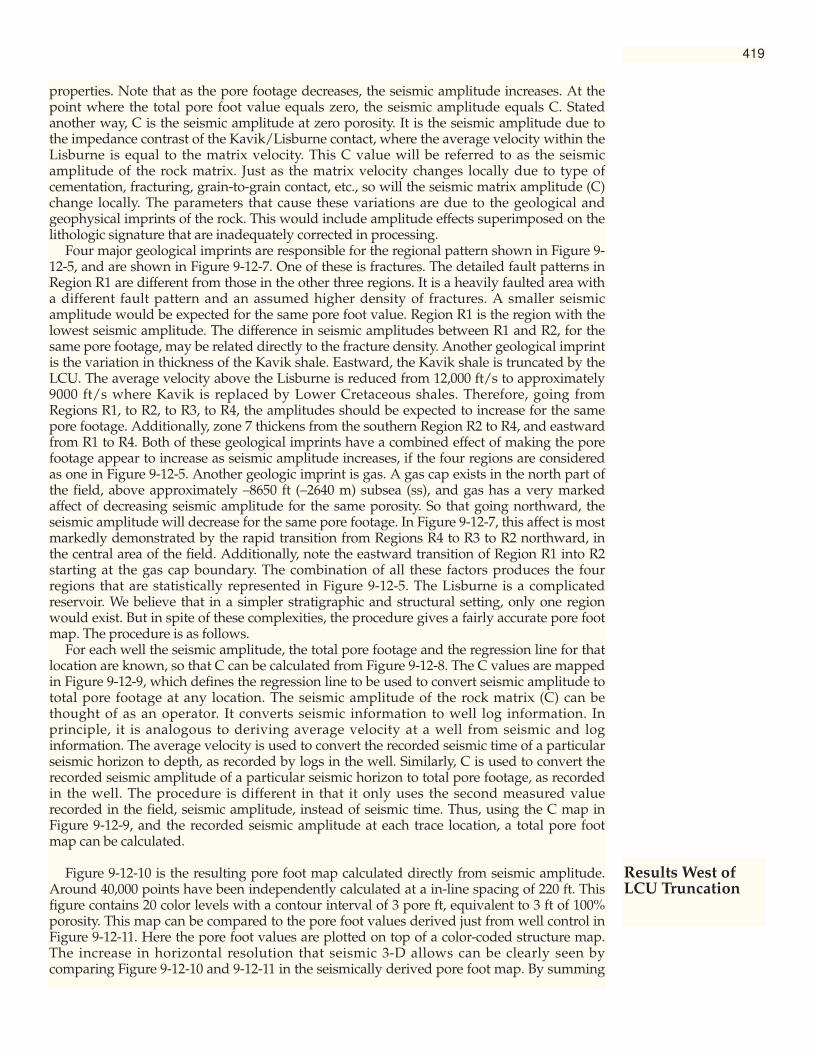
properties. Note that as the pore footage decreases, the seismic amplitude increases. At thepoint where the total pore foot value equals zero, the seismic amplitude equals C. Statedanother way, C is the seismic amplitude at zero porosity. It is the seismic amplitude due tothe impedance contrast of the Kavik/Lisburne contact, where the average velocity within theLisburne is equal to the matrix velocity. This C value will be referred to as the seismicamplitude of the rock matrix. Just as the matrix velocity changes locally due to type ofcementation, fracturing, grain-to-grain contact, etc., so will the seismic matrix amplitude (C)change locally. The parameters that cause these variations are due to the geological andgeophysical imprints of the rock. This would include amplitude effects superimposed on thelithologic signature that are inadequately corrected in processing.

Four major geological imprints are responsible for the regional pattern shown in Figure 9-12-5, and are shown in Figure 9-12-7. One of these is fractures. The detailed fault patterns inRegion R1 are different from those in the other three regions. It is a heavily faulted area witha different fault pattern and an assumed higher density of fractures. A smaller seismicamplitude would be expected for the same pore foot value. Region R1 is the region with thelowest seismic amplitude. The difference in seismic amplitudes between R1 and R2, for thesame pore footage, may be related directly to the fracture density. Another geological imprintis the variation in thickness of the Kavik shale. Eastward, the Kavik shale is truncated by theLCU. The average velocity above the Lisburne is reduced from 12,000 ft/s to approximately9000 ft/s where Kavik is replaced by Lower Cretaceous shales. Therefore, going fromRegions R1, to R2, to R3, to R4, the amplitudes should be expected to increase for the samepore footage. Additionally, zone 7 thickens from the southern Region R2 to R4, and eastwardfrom R1 to R4. Both of these geological imprints have a combined effect of making the porefootage appear to increase as seismic amplitude increases, if the four regions are consideredas one in Figure 9-12-5. Another geologic imprint is gas. A gas cap exists in the north part ofthe field, above approximately –8650 ft (–2640 m) subsea (ss), and gas has a very markedaffect of decreasing seismic amplitude for the same porosity. So that going northward, theseismic amplitude will decrease for the same pore footage. In Figure 9-12-7, this affect is mostmarkedly demonstrated by the rapid transition from Regions R4 to R3 to R2 northward, inthe central area of the field. Additionally, note the eastward transition of Region R1 into R2starting at the gas cap boundary. The combination of all these factors produces the fourregions that are statistically represented in Figure 9-12-5. The Lisburne is a complicatedreservoir. We believe that in a simpler stratigraphic and structural setting, only one regionwould exist. But in spite of these complexities, the procedure gives a fairly accurate pore footmap. The procedure is as follows.

For each well the seismic amplitude, the total pore footage and the regression line for thatlocation are known, so that C can be calculated from Figure 9-12-8. The C values are mappedin Figure 9-12-9, which defines the regression line to be used to convert seismic amplitude tototal pore footage at any location. The seismic amplitude of the rock matrix (C) can bethought of as an operator. It converts seismic information to well log information. Inprinciple, it is analogous to deriving average velocity at a well from seismic and loginformation. The average velocity is used to convert the recorded seismic time of a particularseismic horizon to depth, as recorded by logs in the well. Similarly, C is used to convert therecorded seismic amplitude of a particular seismic horizon to total pore footage, as recordedin the well. The procedure is different in that it only uses the second measured valuerecorded in the field, seismic amplitude, instead of seismic time. Thus, using the C map inFigure 9-12-9, and the recorded seismic amplitude at each trace location, a total pore footmap can be calculated.

Figure 9-12-10 is the resulting pore foot map calculated directly from seismic amplitude.Around 40,000 points have been independently calculated at a in-line spacing of 220 ft. Thisfigure contains 20 color levels with a contour interval of 3 pore ft, equivalent to 3 ft of 100%porosity. This map can be compared to the pore foot values derived just from well control inFigure 9-12-11. Here the pore foot values are plotted on top of a color-coded structure map.The increase in horizontal resolution that seismic 3-D allows can be clearly seen bycomparing Figure 9-12-10 and 9-12-11 in the seismically derived pore foot map. By summing

419

Results West ofLCU Truncation

the pore foot values over the area of concern, the total maximum geological reserves can becalculated, assuming zero water saturation.

For the last three years we have predicted pore foot values from seismic amplitude andcompared them to drilled values. Results have been surprisingly accurate in spite of thecomplexities within the Lisburne. Seismically predicted pore foot values (from Figure 9-12-10) at these 16 new well locations were plotted against the log-measured pore foot values.The results are shown in Figure 9-12-12, which were achieved without updating Figure 9-12-10 after each of the 16 wells were logged.

The previous analysis concentrated on the area west of the truncation where a remnant ofthe Kavik shale still remains. The area east of the truncation is a transitional region whereseismic amplitude would markedly change as a result of the loss of zones 7 through 4, andnot as a result of loss of porosity. The thickness factor in the definition of pore footage ischanging more rapidly than the average porosity factor. To examine the relation of seismicamplitude and pore foot in this area, a geological model was created (Figure 9-12-13). Theresulting seismic amplitude of this synthetic seismic section is shown in Figure 9-12-14. Theresulting peak-to-trough analysis shows that a cyclic pattern develops in the seismicamplitude as a result of the relative positioning of the shales and carbonates in the upperzones as they are being truncated. This cyclic pattern of the synthetic peak-to-trough analysiswill take the shape of a banded structure in map view. The 3-D seismic amplitudes aremapped in Figure 9-12-15 and do appear banded. Again, the red regions are higheramplitudes. Also plotted are the synthetic times between this peak-to-trough event in thelower half of Figure 9-12-14. It, too, has a cyclic pattern, and the 3-D seismic peak-to-troughtime differences also appear as a banded pattern in map view (Figure 9-12-16). Thus, byidentifying the bands on synthetic analysis from wells with known truncated upper zones, aspatial correlation between the synthetic peak-to-trough analysis and the recorded 3-Dseismic peak-to-trough amplitude and times will locate where the zones subcrop against theLCU. These interpreted subcrops are plotted in Figure 9-12-17. Additionally, for areas alongthese subcrops, the total zone thickness is approximately constant so that porosity thicknessvalues could be derived as in the method west of the LCU truncation, in the first part of thiscase history.

Several applications are possible with a detailed seismic pore foot map. One is theconstruction of a truer geologic cross section. For any two wells in the area, only the porositydistribution of those wells is known. The seismically derived pore footage allows boundaryconditions to be set every 220 ft laterally on the interpreted total pore foot distributionbetween these wells. Figure 9-12-18 shows such a porosity distribution between wells L3-08and L3-02. The top of the Lisburne is indicated by the arrow and the red line. Notice that thepeak-to-trough amplitude changes considerably between these two wells, suggesting thatthe total pore footage in zones 7 through 4 is changing at a faster horizontal rate than thegeological cross section would indicate. The seismic cross section seems to indicate that thetotal pore footage is fairly constant for about 4400 ft (1340 m) from L3-08 and then decreasesconsiderably for the next 3300 ft (1000 m). The cycle is repeated several times before L3-02 isreached. This is in contrast to the linear decrease laterally, derived from well values alone,between L3-08 to L3-02. Additionally, by studying the change in the wavelet shape throughperturbing the porosity distribution within each zone separately, the zone of changingporosity can be inferred. For example, a decrease in seismic amplitude with an increase ofpeak-to-trough times is indicative of a zone 6 porosity enhancement. A lower zone 5 porosityenhancement has the same effect with an additional slight side lobe development. Thus, bystudying the amplitude, character, and shape of this wavelet at the top of the Lisburne, amore detailed geologic porosity cross section can be constructed.

Another possible application using a detailed seismic pore foot map is the examination ofthe relation between faults and local pore foot anomalies. Figure 9-12-19 shows theseismically derived pore foot map with a detail fault overlay. Numerous regions areobserved where the fault pattern appears to be directly related to the pore foot anomalies. Inparticular, locations X, O, and the area around E, A, and R. The change in pore footage

420

Method East ofLCU Truncation

Use of Porosity–Thickness Maps

421

around these minor faults (less than 20 ft) may be the result of preservation (or loss) ofsection due to this faulting, or it may be the result of porosity changes due to introduction offluids along related fractures. Thus, local irregularities in the pore foot map can be used tostudy faults and their affects on porosity distribution. Conversely, examining the 3-D seismicat the boundaries of these anomalous pore foot patterns may help locate minor faults nearthe limits of seismic resolution, such as location F (Figure 9-12-19). Only one small lateralfault was interpreted on the east side of this pore foot anomaly. But after careful examination,numerous discontinuous fault segments were linearly mapped on the west side with throwsnear resolution. Additional fault cuts were found on the east side, and the lower boundingnorthwest-extending fault line was projected farther northward. A horst block was thereforeinterpreted to be at location F bounding the anomalous pore foot pattern in Figure 9-12-19.

It is well known that gas has an affect on seismic P-wave velocity, which in thisenvironment decreases amplitude considerably for the same porosity. Figure 9-12-20 is thepeak seismic amplitude map at the Lisburne horizon where blue is the low amplitude andred the high amplitude. The large blue region corresponds well to the original oil-gas contact(–8600 ft) and is within the –8650 ft contour interval. Additionally, other gas caps can befound to the south more than 150 ft deeper within the Lisburne section. If it were possible toreshoot the seismic survey with identically the same acquisition and recording parametersand ground conditions, large amplitude differences between the new and original processedamplitudes should correlate well to unswept, producible oil. Areas therefore may be mappedlocating additional trapped oil.

The final application attempts to relate productivity to total pore foot values for thedrainage area around a well bore, rather than just to the logged pore foot values at the wellbore. Clearly, wells drain areas where the pore footage is not logged but is assumed to have avalue proportional to the linearly weighed distance of the total pore foot difference betweentwo wells. Figure 9-12-21 shows there is a relation between total pore foot and effective porefoot, where the latter term is defined as pore footage with enough permeability to contributeto production (Durfee, 1988). It is a permeability weighted pore foot value. Those wells alongthe upper trend have more effective porosity for the same total pore footage and are alllocated in the truncation areas, or within the gas cap. Figure 9-12-10 then could be multipliedby this ratio and a total effective pore foot map produced. The lower well in Figure 9-12-22shows that production should decrease faster over time than for the more eastern well, eventhough both wells have the same pore footage measured along the well bore. This is due tothe more porous rocks around the eastern well. Production over time at any well then can beequated to the integrated effective seismic pore footage over selected radii from the well, anda set of simultaneous equations generated with factors for fault/fracture enhancements, aswell as rock type.

ARCO Alaska has developed a procedure to calculate porosity-thickness directly from 3-Dseismic amplitude. The procedure uses observed local trends between seismic amplitude andtotal porosity-thickness from wells to project the seismic amplitude that should occur at thatlocation at zero porosity, i.e., for the rock matrix. The geologic and geophysical imprints thataffect this value are complicated and numerous for the Lisburne formation, and yet it wasstill possible to derive an accurate, detailed pore foot map. The procedure is partly anempirical technique which, although it may have wide application, must be locallycalibrated to available well control. The resulting detailed pore foot map serves to enhancereservoir description and assist engineers in developing a more accurate reservoir model.

The techniques and/or conclusions are those of the authoring company and may not beshared by other Working Interest Owners.

Durfee, B. A., 1988, Matrix Characterization of the Upper Wahoo Formation, North Slope,Alaska: ARCO Internal Report, December.

Figures begin on page 422

Conclusions

Reference

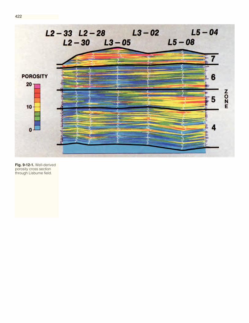
422

Fig. 9-12-1. Well-derivedporosity cross sectionthrough Lisburne field.

423

Fig. 9-12-2. Horizon slicefor top Lisburne reflectiondisplaying peak-to-troughamplitude. Highamplitudes are red; lowamplitudes are blue.

Fig. 9-12-3. Core porosityversus sonic velocity for atypical well.

424

Fig. 9-12-4. Amplitude decreases as porosity increases.

Fig. 9-12-5. Dependence of amplitude on porosity in four regions.

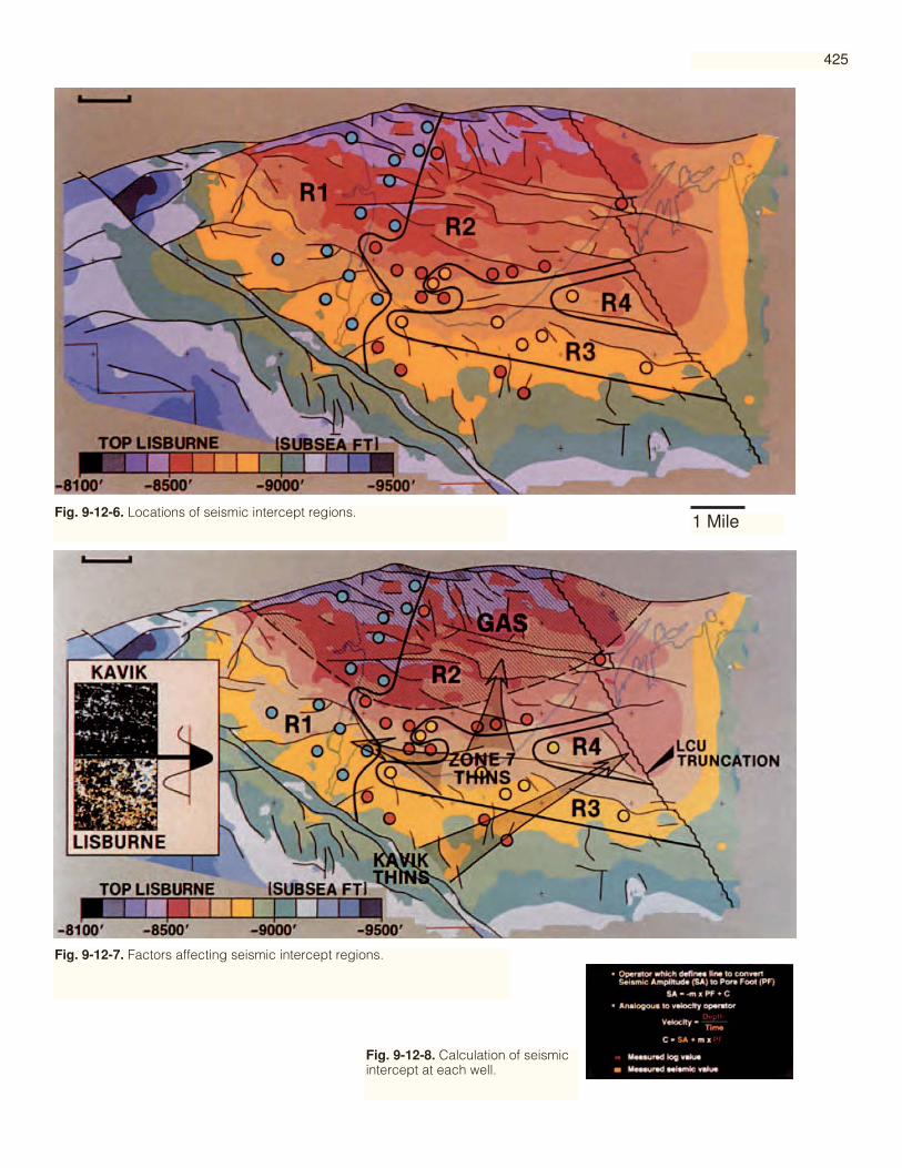
425

Fig. 9-12-6. Locations of seismic intercept regions.

Fig. 9-12-7. Factors affecting seismic intercept regions.

Fig. 9-12-8. Calculation of seismicintercept at each well.

1 Mile

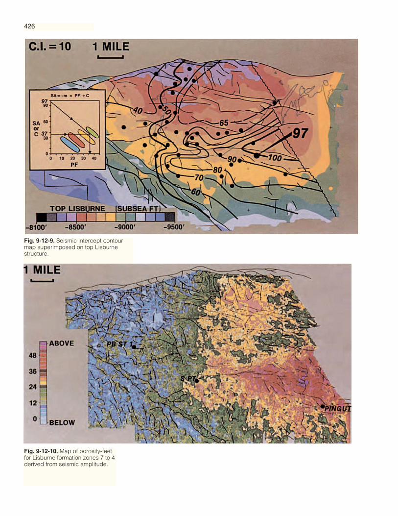
426

Fig. 9-12-10. Map of porosity-feetfor Lisburne formation zones 7 to 4derived from seismic amplitude.

Fig. 9-12-9. Seismic intercept contourmap superimposed on top Lisburnestructure.

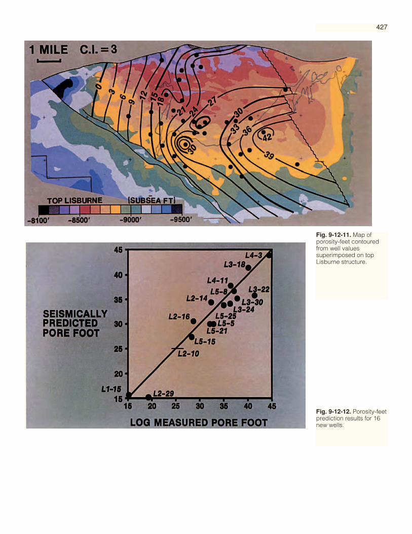
427

Fig. 9-12-11. Map ofporosity-feet contouredfrom well valuessuperimposed on topLisburne structure.

Fig. 9-12-12. Porosity-feetprediction results for 16new wells.

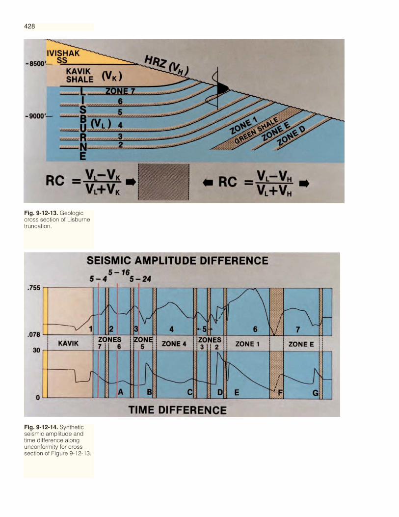
428

Fig. 9-12-13. Geologiccross section of Lisburnetruncation.

Fig. 9-12-14. Syntheticseismic amplitude andtime difference alongunconformity for crosssection of Figure 9-12-13.

429

Fig. 9-12-15. Horizon slice along LowerCretaceous Unconformity, showing bandedpatterns in seismic amplitude.

Fig. 9-12-16. Observed seismic time differencesalong Lower Cretaceous Unconformity, showingbanded patterns.

Fig. 9-12-17. Interpreted truncationssuperimposed on horizon slice of Figure 9-12-15.

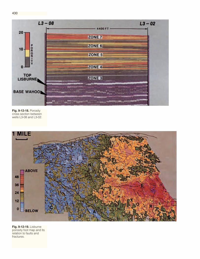
430

Fig. 9-12-18. Porositycross section betweenwells L3-08 and L3-02.

Fig. 9-12-19. Lisburneporosity foot map and itsrelation to faults andfractures.

431

Fig. 9-12-20. Horizonslice for top Lisburnereflection showing lowamplitudes (blue)corresponding to gaszones.

Fig. 9-12-21. Effectiveporosity foot versus totalporosity-feet.

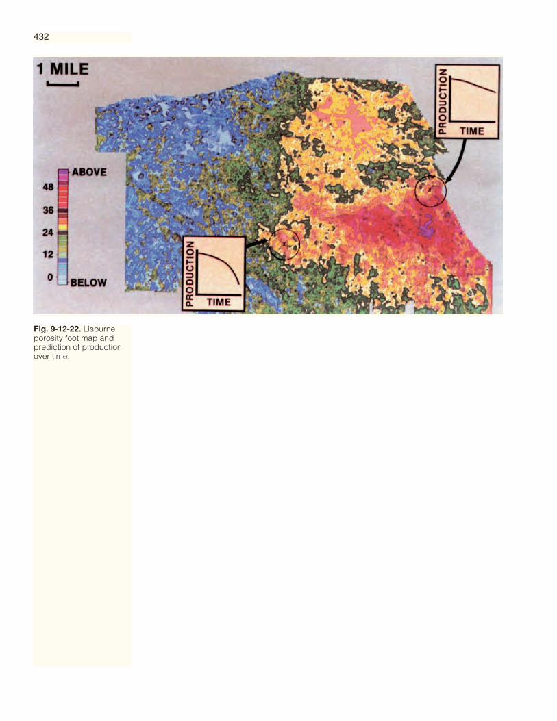
432

Fig. 9-12-22. Lisburneporosity foot map andprediction of productionover time.

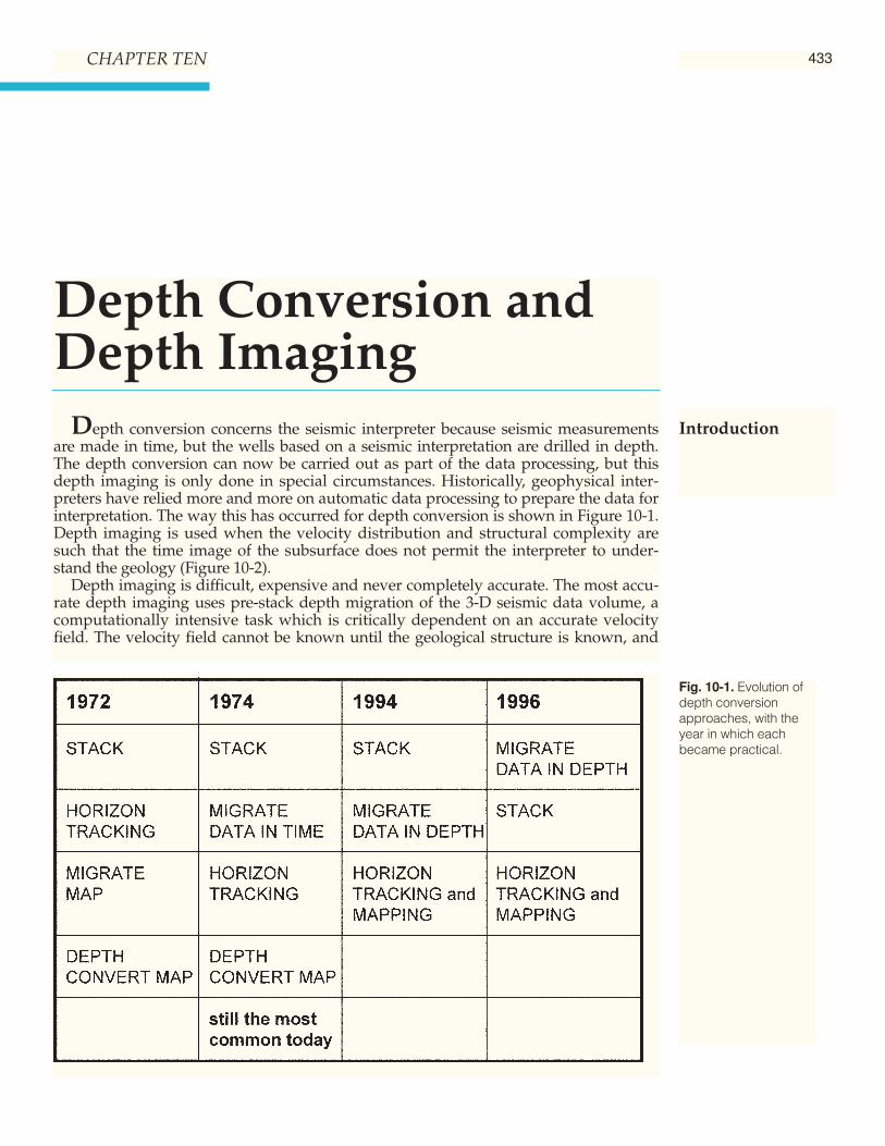
433

Depth Conversion andDepth Imaging

Depth conversion concerns the seismic interpreter because seismic measurementsare made in time, but the wells based on a seismic interpretation are drilled in depth.The depth conversion can now be carried out as part of the data processing, but thisdepth imaging is only done in special circumstances. Historically, geophysical inter-preters have relied more and more on automatic data processing to prepare the data forinterpretation. The way this has occurred for depth conversion is shown in Figure 10-1.Depth imaging is used when the velocity distribution and structural complexity aresuch that the time image of the subsurface does not permit the interpreter to under-stand the geology (Figure 10-2).

Depth imaging is difficult, expensive and never completely accurate. The most accu-rate depth imaging uses pre-stack depth migration of the 3-D seismic data volume, acomputationally intensive task which is critically dependent on an accurate velocityfield. The velocity field cannot be known until the geological structure is known, and

Fig. 10-1. Evolution ofdepth conversionapproaches, with theyear in which eachbecame practical.

CHAPTER TEN

Introduction

434

the geological structure cannot be known until the seismic volume has been migrated.Consequently, the depth imaging process usually involves iteration.

Depth conversion of a time interpretation, on the other hand, is computationally sim-ple, and can be quickly repeated whenever new information becomes available. Themost common procedure for preparing a depth image of the earth from 3-D seismicdata is to time-migrate the 3-D data volume, usually after stack, and convert the timeinterpretation into a depth model of the earth. Accurate depth conversion is particularlyimportant because the 3-D data volume presents the promise of much more reliableinterpretation than with 2-D seismic methods, so errors in depth conversion can be thelargest errors in the final interpretation.

The physical quantity that relates time to depth is velocity. In most seismic interpreta-tion, we are concerned with the velocity of compressional (P) waves through the earth,because conventional seismic processing attempts to eliminate all seismic energy exceptthat which represents a simple P-wave reflection. The velocity required for convertingtime to depth is the P-wave velocity in the vertical direction. It can be measured directlyin a well, or extracted indirectly from surface seismic measurements, or deduced from acombination of seismic and well measurements. Conventional time-to-depth conver-sion is the subject of the first half of this chapter.

INC

RE

AS

ING

ST

RU

CT

UR

AL

CO

MP

LE

XIT

Y

PRE-STACKTIME

PRE-STACKDEPTH

POST-STACKDEPTH

POST-STACKTIME

INCREASING VELOCITY VARIATION

Fig. 10-2. Appropriatekind of migration as afunction of structure andvelocity variation (afterLiner, 1996).

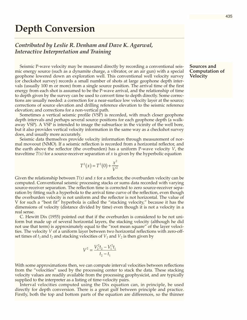
Depth Conversion

Contributed by Leslie R. Denham and Dave K. Agarwal, Interactive Interpretation and Training

Seismic P-wave velocity may be measured directly by recording a conventional seis-mic energy source (such as a dynamite charge, a vibrator, or an air gun) with a specialgeophone lowered down an exploration well. This conventional well velocity survey(or checkshot survey) records a small number of shots at large geophone depth inter-vals (usually 100 m or more) from a single source position. The arrival time of the firstenergy from each shot is assumed to be the P-wave arrival, and the relationship of timeto depth given by the survey can be used to convert time to depth directly. Some correc-tions are usually needed: a correction for a near-surface low velocity layer at the source;corrections of source elevation and drilling reference elevation to the seismic referenceelevation; and corrections for a non-vertical path.

Sometimes a vertical seismic profile (VSP) is recorded, with much closer geophonedepth intervals and perhaps several source positions for each geophone depth (a walk-away VSP). A VSP is intended to image the subsurface in the vicinity of the well bore,but it also provides vertical velocity information in the same way as a checkshot surveydoes, and usually more accurately.

Seismic data themselves provide velocity information through measurement of nor-mal moveout (NMO). If a seismic reflection is recorded from a horizontal reflector, andthe earth above the reflector (the overburden) has a uniform P-wave velocity V, thetraveltime T(x) for a source-receiver separation of x is given by the hyperbolic equation

Given the relationship between T(x) and x for a reflector, the overburden velocity can becomputed. Conventional seismic processing stacks or sums data recorded with varyingsource-receiver separation. The reflection time is corrected to zero source-receiver sepa-ration by fitting such a hyperbola to the arrival time curve of the reflection, even thoughthe overburden velocity is not uniform and the reflector is not horizontal. The value ofV for such a “best fit” hyperbola is called the “stacking velocity,” because it has thedimensions of velocity (distance divided by time) even though it is not a velocity in areal sense.

C. Hewitt Dix (1955) pointed out that if the overburden is considered to be not uni-form but made up of several horizontal layers, the stacking velocity (although he didnot use that term) is approximately equal to the “root mean square” of the layer veloci-ties. The velocity V of a uniform layer between two horizontal reflections with zero-off-set times of t1 and t2 and stacking velocities of V1 and V2 is then given by

With some approximations then, we can compute interval velocities between reflectionsfrom the “velocities” used by the processing center to stack the data. These stackingvelocity values are readily available from the processing geophysicist, and are typicallysupplied to the interpreter as a listing of time-velocity pairs.

Interval velocities computed using the Dix equation can, in principle, be useddirectly for depth conversion. There is a great gulf between principle and practice.Firstly, both the top and bottom parts of the equation are differences, so the thinner

Sources andComputation ofVelocity

435

T x TxV

2 22

20( ) = ( ) +

VV t V t

t t2 2

22 1

21

2 1

=−−

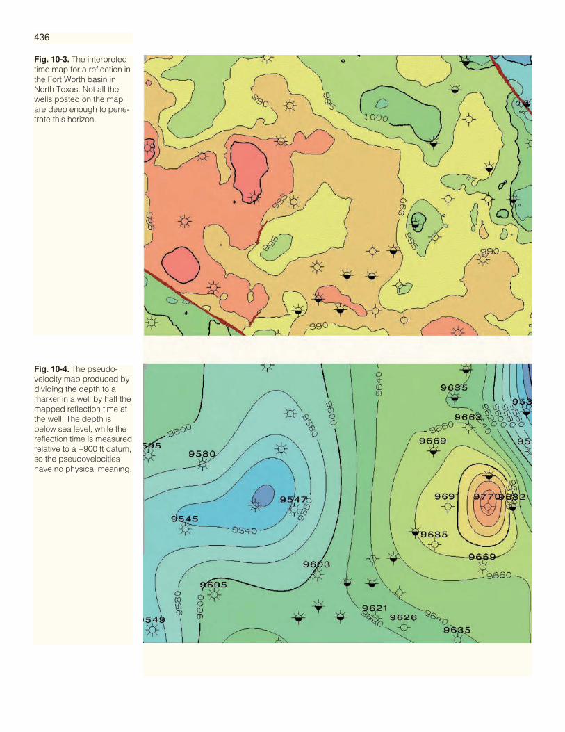
Fig. 10-3. The interpretedtime map for a reflection inthe Fort Worth basin inNorth Texas. Not all thewells posted on the mapare deep enough to pene-trate this horizon.

Fig. 10-4. The pseudo-velocity map produced bydividing the depth to amarker in a well by half themapped reflection time atthe well. The depth isbelow sea level, while thereflection time is measuredrelative to a +900 ft datum,so the pseudovelocitieshave no physical meaning.

436

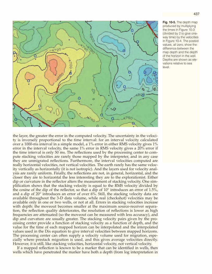
the layer, the greater the error in the computed velocity. The uncertainty in the veloci-ty is inversely proportional to the time interval: for an interval velocity calculatedover a 1000-ms interval in a simple model, a 1% error in either RMS velocity gives 1%error in the interval velocity, the same 1% error in RMS velocity gives a 20% error ifthe time interval is only 50 ms. The reflections used by the processing center to com-pute stacking velocities are rarely those mapped by the interpreter, and in any casethey are unmigrated reflections. Furthermore, the interval velocities computed arereally horizontal velocities, not vertical velocities. The earth rarely has the same veloc-ity vertically as horizontally (it is not isotropic). And the layers used for velocity anal-ysis are rarely uniform. Finally, the reflections are not, in general, horizontal, and thecloser they are to horizontal the less interesting they are to the explorationist. Eitherdip or curvature in the reflector alters the measurement of stacking velocity. One sim-plification shows that the stacking velocity is equal to the RMS velocity divided bythe cosine of the dip of the reflector, so that a dip of 10° introduces an error of 1.5%,and a dip of 20° introduces an error of over 6%. Still, the stacking velocity data areavailable throughout the 3-D data volume, while real (checkshot) velocities may beavailable only in one or two wells, or not at all. Errors in stacking velocities increasewith depth: the moveout becomes smaller at the maximum source-receiver separa-tion, the reflection quality deteriorates, the resolution of reflections is lower as highfrequencies are attenuated (so the moveout can be measured with less accuracy), anddip and curvature are usually greater. The stacking velocity pairs given by the pro-cessing center provide a function of stacking velocity as a function of depth, and thevalue for the time of each mapped horizon can be interpolated and the interpolatedvalues used in the Dix equation to give interval velocities between mapped horizons.The processing center can often supply a velocity volume used for migration, espe-cially where prestack migration is used, and this gives average velocities directly.However, it is still, like stacking velocities, horizontal velocity, not vertical velocity.

If a mapped reflection is known to be a marker that can be identified in wells, thenwells which have penetrated the marker have both a depth (from log interpretation in

Fig. 10-5. The depth mapproduced by multiplyingthe times in Figure 10-3(divided by 2 to give one-way time) by the velocitiesin Figure 10-4. The postedvalues, all zero, show thedifference between themap depth and the depthof the horizon in the well.Depths are shown as ele-vations relative to sealevel.

437

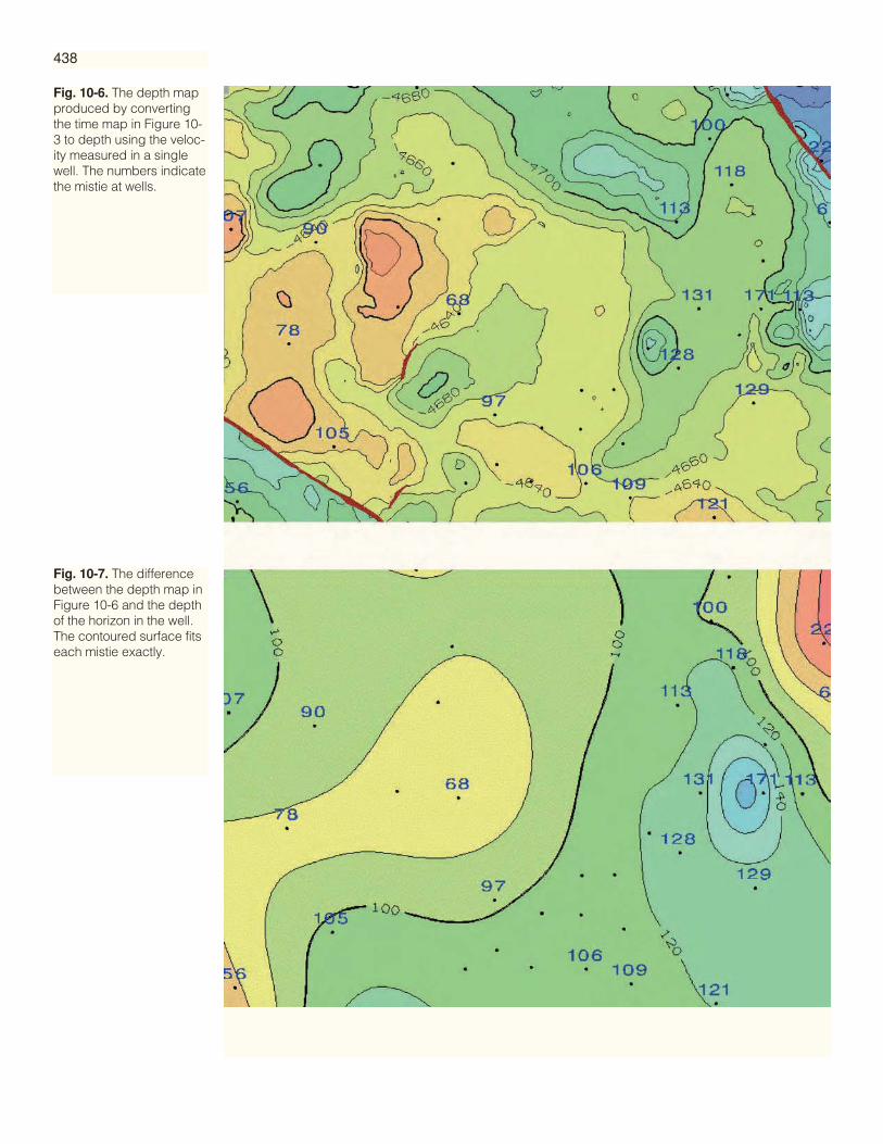
Fig. 10-6. The depth mapproduced by convertingthe time map in Figure 10-3 to depth using the veloc-ity measured in a singlewell. The numbers indicatethe mistie at wells.

Fig. 10-7. The differencebetween the depth map inFigure 10-6 and the depthof the horizon in the well.The contoured surface fitseach mistie exactly.

438

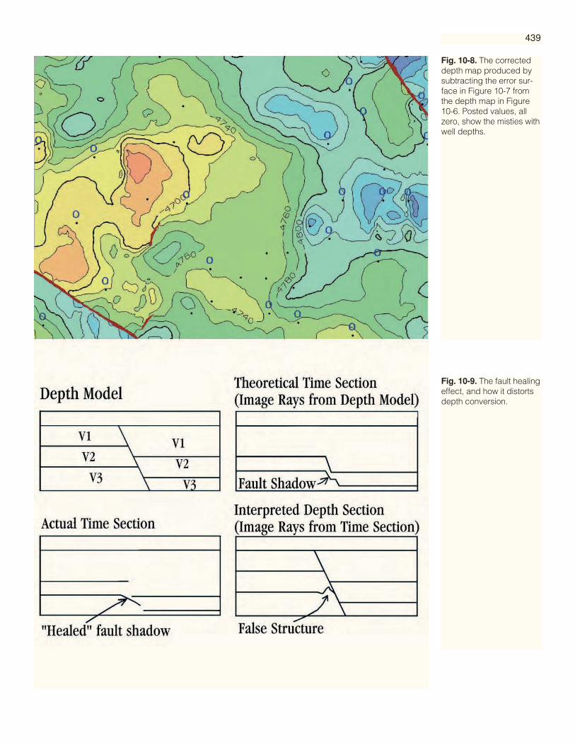
Fig. 10-8. The correcteddepth map produced bysubtracting the error sur-face in Figure 10-7 fromthe depth map in Figure10-6. Posted values, allzero, show the misties withwell depths.

Fig. 10-9. The fault healingeffect, and how it distortsdepth conversion.

439

the well) and a time (from the 3-D seismic interpretation). Figure 10-3 shows a timemap over an area with about 20 wells that have penetrated the mapped marker. If wedivide the depth below datum of the marker by the interpreted time at the well, wehave calculated an empirical velocity, often termed “pseudovelocity,” which will con-vert the time of this event to the depth of the well marker at this well. With enoughwells, we can map changes of the pseudovelocity, so that a velocity is available over thewhole of the survey as shown in Figure 10-4. The depth map (Figure 10-5) computedfrom the interpreted time map and the pseudovelocity map, must tie exactly at eachwell used for pseudovelocities, but there is no way of estimating the accuracy of themap away from these wells.

Geostatistical cokriging is a statistical technique for using a measured value of onequantity at many points to estimate the value of another quantity at those many points,given a few measurements of the second quantity. Because depth is closely related totime the technique works quite well for direct conversion of time to depth without com-puting velocity. The results are very similar to using pseudovelocities, with the advan-tage of giving an estimate of the accuracy of the final depth map, but this requires spe-cial software. Geostatistical software has not been integrated into commonly usedinterpretation or mapping systems, and stand-alone geostatistical software tends tohave user manuals and a user interface that only a mathematician could love (Wolf,1990).

Velocities may be available from several sources: well velocity surveys, VSPs, stack-ing velocities, and pseudovelocities. The interpreter typically combines them by usingthe sparse, accurate data points at wells to calibrate maps generated from numerous butless accurate stacking velocity measurements. Often the interpreter must reject anoma-lous values, using the criteria of geological reason. The final velocity field used fordepth conversion must represent a reasonable approximation to the geological modelrepresented by the final interpretation. Velocities must be realistic for the lithologiesknown or presumed to be present, and any lateral or vertical changes in velocity musthave a geological explanation.

The velocities available for depth conversion may have varying accuracy. Actualmeasurements in a well, whether a velocity survey or a VSP, are usually very accurate,with errors often as small as 0.1% or better, but velocities computed from moveout areoften in error by 5% or more. One of the subtler characteristics of time migrated data isthat a vertical line through the time-migrated data volume (along the time axis) doesnot necessarily represent a vertical line through the earth. In fact, it only represents avertical line through the earth when there is no horizontal velocity gradient, when allisovelocity surfaces are horizontal. This was first published by Peter Hubral (1977). Inother cases, the true position of a point on a time-vertical trace can be found by tracingthe ray into the earth from the surface (or from the seismic datum plane), starting with avertical ray and bending it according to Snell’s Law at all velocity boundaries. This pro-cess is called “image ray migration.”

If there is an abrupt lateral change in velocity, as at a fault, the approximation that thestacked seismic trace is the same as the zero-offset seismic trace, and that the migratedseismic trace represents data along an image ray, would lead the interpreter to expect adiscontinuity in deeper reflections, a “fault shadow,” even when they are not faulted(Figure 10-9). In real data, any discontinuity disappears rapidly with increasing depthbelow the discontinuous velocity surface: the samples which make up the time-migrat-ed trace come from the stacked data volume within a cone expanding upwards fromthe sample time, so samples below the discontinuity soon include data from both sides.In effect, the fault shadow is “healed” with depth, becoming a broader and broadermonocline.

When using any layer-based depth conversion technique, we must simulate this fault

GeneralConsiderations in

Depth Conversion

440

shadow healing by smoothing a layer before building downwards from it. A techniquethat works well is to remove wavelengths shorter than the layer thickness, from boththe time and the depth maps of the top of the layer. The exact tie of a well to a seismictrace should be represented by the synthetic seismogram computed from sonic anddensity logs in the well, calibrated by a velocity survey or a VSP. In real life, the synthet-ic seismogram is rarely a good match to the processed seismic trace. The well tie of areflection is usually best determined by answering two questions:

Is there a noticeable change in acoustic impedance as measured by the well logs atabout the correct time as defined by velocity survey?

Is the mapped seismic event of the expected polarity for the direction of change ofthe acoustic impedance, taking into account the polarity conventions assumed by theprocessing center, and the phase manipulations in the processing sequence?

If the answer to both of these questions is “yes”, then the mapped event probablyrepresents the acoustic impedance change. If either answer is “no”, the mapped eventmay not be reliably identified. If a horizon can be accurately identified at one well, andis reliably identified throughout the survey by its distinctive character, it will in mostareas be correct to assume that it is the same geological marker throughout the area.However, seismic reflections in general follow geological time lines, often representingthin but persistent chronostratigraphic units representing widespread geological phe-nomena such as maximum sea level fluctuations or volcanic eruptions. On the otherhand, the formations identified in wells by geologists are often lithostratigraphic units,which may or may not have been deposited at the same time throughout the area.

Many small 3-D interpretations can be converted from time to depth using a singlevelocity function, often from a velocity survey in one well, either in the area of the 3-Dsurvey or nearby. Such a function is usually a series of time-depth pairs, with the timerecorded from the surface to several widely-spaced points down the well. Depth con-version uses the grid manipulation functions of the mapping system. Because these areusually limited to a few arithmetic operations, the interpreter often approximates themeasured time-depth function with a mathematical function such as a straight line fit-ted to the time-depth points within the time range of the time map. A non-linear time-depth function may also be used, and could be any mathematical expression which fitsthe data and which can be evaluated using the grid manipulation functions of the map-ping system.

The results of such a conversion are shown in Figure 10-6. Because the measuredtime-depth function is accurate only at one point (the well where it was recorded), thedepth map does not usually tie to the depths for the mapped formation measured inother wells. To correct for the mistie, the interpreter can fit a smooth surface to the mis-tie values, shown in Figure 10-7, and subtract this surface from the depth map to give acorrected depth map, Figure 10-8, which ties exactly at each well.

Where several wells have velocity surveys, or where other methods provide veloci-ties, some way of handling the varying velocities must be used. The easiest way to dothis is to map the velocity in some way: either the actual average velocity at each point(as was done in Figure 10-4) or constants in the velocity function fitted to the datapoints at each well. If a straight line time-depth function of the form Z=a + bT is used,where Z is depth and T is time and a and b are constants, the interpreter could mapeither a or b, and hold the other constant over the whole area, or could map both of theconstants. With both constants mapped, the depth map would be produced by multi-plying the time map grid by the b map grid, and adding the a map grid. This depthmap requires residual corrections in the same way as the map prepared using a singlevelocity function, unless the only velocities used are pseudovelocities.

Depth ConversionUsing a SingleVelocity Function

Depth ConversionUsing MappedVelocity Function

441

Fig. 10-10. The interpretedtime map for a shallowhorizon marking theboundary between twovelocity layers.

Fig. 10-11. A depth mapproduced by conversionfrom time to depth in twolayers. The velocity usedfrom seismic datum to thehorizon mapped in Figure10-10 is 10204 ft/s, andthe velocity used from thisshallow horizon to the hori-zon shown in Figure 10-3is 12107 ft/s. A constantcorrection of -208 ft wasapplied to give an averagemistie of zero, and theposted values show theresidual misties. The stan-dard deviation of the mis-ties is 30 ft.

442

Fig. 10-12. A third ordertrend surface fitted to theresidual errors shown inFigure 10-11.

Fig. 10-13. The correcteddepth map produced bysubtracting the trend sur-face in Figure 10-12 fromthe depth map in Figure10-11. The residual mistiesare posted on the map.The standard deviation ofthe residual mistie is 18 ft.

443

Where there are major velocity changes in the overburden which result largely fromchanges in lithology rather than from depth of burial, interpolation between controlpoints should use a series of layers with different velocities for each layer. The simplestcase is where the velocity for each layer is constant. In this case, the interval from thesurface to the base of the first layer is converted to depth using one of the methodsdescribed above. Then the time interval over the next layer is converted to a depthinterval using a constant velocity (or single velocity function) and added to the depth tothe base of the first layer to give the depth to the base of the second layer, and the pro-cess repeated for each subsequent layer. Figure 10-10 shows the time map for a shallowreflection marking a major velocity break. At the one well with a velocity survey, thevelocity for the interval above the shallow reflection is 10204 ft/s, and from that reflec-tion to the deep reflection (Figure 10-3) the velocity is 12107 ft/s. The depth map fromthe layer method, with a constant added to give zero average mistie, is Figure 10-11.

If there were significant faulting in the shallow layer, we would need to smooth thetime map for the top of each layer before computing the time interval, and the depthmap for the top of each layer before adding the depth interval. This is to remove theeffect of “fault healing”, shown in Figure 10-9. Abrupt lateral changes in velocity in theoverburden, such as might occur at a fault, should produce apparent faulting in deeperreflectors; but in real seismic data this effect is rarely seen. The time migration process,where recorded data from both sides of an abrupt velocity variation are used to pro-duce the migrated image below the anomaly, mixes data actually recorded over a circu-lar area above the imaged subsurface point.

Lateral velocity variations in the layers are accommodated in the same way that theyare in a single layer case: by mapping the variations, either directly as variations in thevelocity over the interval of the layer, or by variations in parameters of a mathematicalfunction. As for a single layer, the velocity may change with depth. However, suchfunctions introduce complications in depth conversion. The time map to be convertedto depth must be the pseudotime map that would be recorded if the velocity functionfor the layer held for the total depth interval from the survey datum to the base of thecurrent layer. If there are abrupt lateral thickness changes in the shallower section, thesemust be smoothed out to simulate the smoothing inherent in processing. The procedurethen for each layer is this:

1. Smooth time and depth maps for the top of the layer.2. Convert the smoothed depth map to the top of the layer to a pseudotime map,

using the (possibly mapped) time-depth function for the layer.3. Compute the time interval from the smoothed time map at the top of the layer to

the unsmoothed time map of the base of the layer.4. Add this time interval to the pseudotime map for the top of the layer to give a

pseudotime map for the base of the layer.5. Convert this pseudotime map to depth using the (possibly mapped) time-depth

relationship for the layer.As with the single-layer case, the final map will not tie to the wells. The constant part ofthe error is easily removed, as in Figure 10-11, and the residual error can either be left inthe final map or removed by subtracting an error grid as in Figure 10-7.

Where the Hubral effect becomes significant, usually where the dip on velocity inter-faces exceeds about 15°, the most accurate solution to depth conversion of a time map isimage-ray migration. This is done with map-migration software designed for the pur-pose starting with a horizon map picked on unmigrated data. The magnitude of theHubral effect can be calculated by applying Snell’s Law to a ray projected verticallydown from the surface through the velocity structure proposed for depth conversion.

In principle, an interpreter could produce a more accurate map of a complex area byinterpreting unmigrated seismic data and using map migration. In real exploration situ-ations, this is almost always impossible, because crossing reflections become impracti-cal to map. Where this approach might have been the only way of resolving complex

Map Migration

444

Depth ConversionUsing Layers

Fig. 10-14. Differencebetween the depth mapsof Figure 10-5, generatedusing pseudovelocities,and Figure 10-8, generat-ed using a single velocityfunction.

Fig. 10-15. Differencebetween the depth mapsof Figure 10-5, generatedusing pseudovelocites,and Figure 10-11, gener-ated using layers. Notethat this map is not verysimilar to Figure 10-14.

445

structure with 2-D seismic exploration, 3-D seismic surveys allow 3-D depth migration,which, although expensive, may be the only practical technique where velocity struc-ture is complex. Depth imaging is discussed in the next part of this chapter.

All the depth conversion methods described here, with the exception of the pseu-dovelocity method, fail to tie exactly at wells. The amount of this well mistie can showhow accurate the map is likely to be away from the well ties, where a new well is likelyto be drilled. The constant component of all well misties should be subtracted from thedepth map to give a map such as Figure 10-8 where the average mistie is zero. Theresidual misties are a measure of the accuracy of the final map. The misties posted onthe map in Figure 10-11 have a standard deviation of 30 ft. In other words, a well drilledhas a 95% chance of finding the mapped formation within 60 ft of the mapped depth.For a map with a total range of 220 ft, that is not reassuring.

The estimated errors for a map can be reduced in several ways. Firstly, some of themisties may be incorrect because either the depth in the well is incorrect, or because theinterpreter has picked locally on the wrong reflection. The interpreter should checkcarefully both the seismic interpretation and the well depth at any wells where the mis-tie is much larger than average. Once this possibility has been eliminated, the remain-ing errors may be largely due to errors in the velocities, usually due to inadequate con-trol points. Such errors could be expected to vary slowly across the map, so fitting asmooth trend to the misties should correct for them. Figure 10-12 is an example of suchan error trend. Subtracting this error produced the corrected depth map in Figure 10-13.The standard deviation of the errors posted on this map is 18 ft, a significant improve-ment.

Once the interpreter has made a best estimate for a corrected depth map, there arestill misties at wells. A final presentation map that has no errors at wells is made bygridding a residual error surface from the final misties, and subtracting this from thefinal depth map. Persons using this map must not assume that just because it shows thecorrect depth at all the wells it is completely accurate. Both Figure 10-5 and Figure 10-8tie all the wells exactly. But they are not the same maps. The difference between the twois shown in Figure 10-14. The most accurate uncorrected map shown for this project ispossibly Figure 10-11 and the difference between this and Figure 10-5 is shown in Fig-ure 10-15. This difference map shows little resemblance to the trend surface used torefine the depth conversion to produce Figure 10-13. The comparison underscores thedifficulty in evaluating the accuracy of any depth conversion.

The very nature of seismic data, recorded in a typical nonisotropic medium, doesnot permit the derived depth surface to be accurate at all points in a given area. Someadvantages and disadvantages of each technique are:

• Depth conversion with a single velocity function may be satisfactory over a verylimited area, perhaps just around the well where the velocity data were acquired;this method often minimizes local errors in absolute depth for a single horizon.

• Where velocities vary with depth of burial more than with stratigraphic units,using a mapped velocity function is often the simplest and most accurate tech-nique.

• Pseudovelocities and other techniques which convert each horizon independent-ly often give small absolute errors for each horizon, but if the horizons are closelyspaced the intervals can be grossly in error: the interpreter may even producemaps which imply crossing horizons.

Discussion

446

Dealing withConversion Errors

• Image-ray map migration suffers from errors in velocities and the assumptionthat the stacked seismic trace is a zero-offset trace, but it may be needed in areaswith both steep dip and large velocity variations.

• The layer-cake method minimizes the errors in the thickness of individual layersbut may introduce large errors in the cumulative depth when several layers areadded together. This velocity model is geologically more realistic where velocitieschange rather abruptly across the stratigraphic boundaries, but less realisticwhere velocity variation depends more on depth of burial than on stratigraphicposition. Most commercial software packages appear to use this technique, some-times with image-ray map migration as an option. Layer-cake depth conversionhas two disadvantages:

1. Abrupt horizontal changes in velocity often produce false structures in theunderlying horizons.

2. This technique is unnecessarily complex and prone to errors where velocityis more a function of depth of burial than of stratigraphy.

The best one can do is to make full use of the available velocity data and to ensurethat all information available in each well is fully consistent with the geophysicalinterpretation within the statistical probable error. The interpretation must not beforced to tie exactly to the well information; the most accurate depth surface is theone that statistically gives a minimum standard deviation. Statistical adjustmentsensure that the residual misties are a true indication of the accuracy of the interpreta-tion. Depth conversion software packages often ease the mechanics of complex depthconversion techniques, but the interpreter must understand exactly how the softwareworks before relying on the output.

Dix, C. H., 1955, Seismic velocities from surface measurements: Geophysics, v. 20, p. 68-86.

Hubral, P., 1977, Time migration — some ray-theoretical aspects: Geophysical prospect-ing, v. 25, p. 738-745.

Liner, C. L., 1996, Seismos — a free-form column on the history and culture of geo-physics: The Leading Edge, v. 15, p. 1156-1158.

Wolf, D. J., 1990, Mathematics and geostatistics: A Tutorial for geoscientists without thePh.D. in mathematics (geostatistics for poets): SEG 60th Annual Meeting expandedabstracts, p. 336-338.

447

References

3-D Depth Image Interpretation

Contributed by William L. Abriel, Joseph P. Stefani, Robert D.Shank, and David C. Bartel, Chevron U.S.A.

The purpose of our paper is to illustrate the concept of 3-D depth imaging inseismic exploration and development. Our experience is concentrated in the Gulfof Mexico subsalt where depth imaging is an integral part of that play. Through theuse of models and live data examples, it is our intent to communicate why andhow depth imaging works, as well as some of the pitfalls.

Depth imaging has grown significantly in the past decade as a percent of theseismic processing industry. Geologists, engineers and geophysicists are more com-monly utilizing depth-imaged seismic data in daily activities to find and under-stand hydrocarbon reservoirs. And although the tradition of depth imaging growsfrom interests in structural definition of hydrocarbon traps, the quality of depthimaging in 3-D is high enough to also have significant impact in reservoir defini-tion and stratigraphic imaging. As depth imaging moves further into the main-stream of our business, it becomes important to describe and even quantify theuncertainties of the earth descriptions we derive from these data.

It is not necessary for users of depth images to be high-powered seismic dataprocessors. However, it is important for users to understand the required elementsof successful depth imaging, and how these elements contribute to the success orfailure of the imaging process. One very important concept that needs to be under-stood is the sensitivity of seismic imaging to variations in overlying earth velocity,and why depth images can be significantly different from time-imaged data. Anextension of this concept also shows why 3-D pre-stack depth imaging may be nec-essary instead of post-stack. Another signal-based concept requiring clear under-standing is that of incomplete seismic illumination in shadow zones. These mustnot be mistaken for changes in reflection amplitude variation caused by changes inlithology, fluids or pressure. In addition to understanding the signal concepts, it isalso important to understand coherent noise and how it should appear in depth-imaged data.

The models and data examples shown in the sections that follow are intended toillustrate the above points. In order to cover them all, we have compiled data froma series of different projects. We have concentrated on illustrating one play type(Gulf of Mexico subsalt) for consistency and focus. The basic concepts illustratedhere are useful when understanding other plays where depth imaging is used, butit should be noted that the relative importance of the elements constituting depthimaging varies among plays.

The imaging of seismic data is intended to represent the earth subsurface reflec-tivity with sufficient accuracy for rendering structural geology, stratigraphy, andreservoir properties. Field data are recorded in the time domain with varyingsource-receiver offsets to reflect energy from the subsurface at multiple angles.

Time imaging of these data attempts to add together the subsurface reflectionsand position (migrate) them to the appropriate 3-D xyz positions while still retain-ing time as the z axis. Time imaging generally employs elements of a “flat earth”processing model, and cannot correct for rapid variations in earth velocity. There-fore time imaging is forgiving of small earth-model errors but fails when velocity

449

Concept of 3-DDepth Imaging

Why TimeImaging Is NotDepth Imaging

varies rapidly. Standard practice of using these time data is to interpret them in thetime domain, and convert the resulting map to depth, as described in the first partof this chapter. Alternately, the seismic time data are depth “stretched” either verti-cally or along raypaths dictated by the velocity model. However, depth stretchingof traces should not be confused with depth imaging.

Depth imaging uses a velocity model in the depth domain to compensate forpropagation effects. Each vertical and horizontal change in the velocity field ishonored in a specialized migration algorithm to account for the bending of theenergy down to reflection wavelength scales. In this sense, depth imaging is a cor-recting lens attempting to place the reflected energy in its correct xyz depth posi-tion. Although costlier, depth imaging is generally more accurate than time imag-ing. As a result, depth imaging is fast becoming the process of choice in areas ofhigh velocity complexity.

But along with the increase in image accuracy, comes the danger of not havingthe right earth velocity to make the corrections. Because depth imaging does suchexact calculations of the ray paths, it is very sensitive to errors in our intervalvelocity model of the earth. While small distributed errors in spatially smooth RMSvelocities are generally not harmful in time migration, cumulative errors in thelocal interval velocity are leveraged and magnified in the depth imaging process.These can be so bad as to degrade the depth image to the extent that it gives lessinformation than a depth stretch of the time-imaged data! Depth imaging, then,must be considered in a context much wider than a migration algorithm, and mustat least also include velocity analysis, accuracy, and representation.

As a representation of the principles behind depth imaging, refer to the model ofseismic ray propagation in Figure 10-16. The 2-D cross-section shows a salt ledgeburied in sediments of modest velocity variation represented by multicolored lay-ers. Imaging of the subsurface typically employs seismic traces from shots andreceivers whose midpoint at the surface is the same (common mid point: CMP).This allows subsurface reflection points (common reflection point: CRP) to addtogether when the earth velocity can be approximated by flat layers. However,when the earth velocity layers are not very flat, the subsurface reflection points arenot in common, and the image can become seriously distorted.

In Figure 10-16, the individual CMP rays in black illustrate how the seismicenergy travel path through sediments suffers small “kinks” at the interfaces wherethe velocity changes. In contrast, at the salt boundaries the change in angle is quitelarge, and so this body acts as a distorting lens for imaging the reflectors below.The cross-section shows how rays constituting a single CMP gather hit the subsur-face irregularly over a 5000-foot horizontal area. The theory for time imaging gen-erally assumes that the kinks are small and not important at the small scale. It alsoassumes that no large ray bending occurs like we see at the salt interfaces.

The inset in Figure 10-16 helps illustrate this difference in time and depth imag-ing. The plot of offset versus time shows the ray arrivals as recorded at the surface.Ideal time imaging requires the arrivals to fall along a hyperbola, but complex raybending scatters individual arrivals about a hyperbolic trajectory. In this case timeimaging is unsatisfactory, precisely because it assumes straight rays, and because itfurther assumes the reflection comes from the horizontal location of the midpointat x = 15,000 feet.

Correct depth imaging, however, is designed to correct for these distortions andplace the events in their appropriate horizontal and vertical position. The effect ofdepth imaging is to use the source-receiver pairs whose common reflection pointsare the same, based on good knowledge of the velocity through which the raystravel. The small kinks are honored directly, and all ray bending is taken intoaccount. Where no salt exists in Figure 10-16, the rays generally make it to the sur-face without much distortion. Through the salt, however, the salt/sediment veloci-ty contrast of 2 has a large effect where the rays intersect the salt interface at a non-normal angle. Rays can emerge from the salt displaced thousands of feet

450

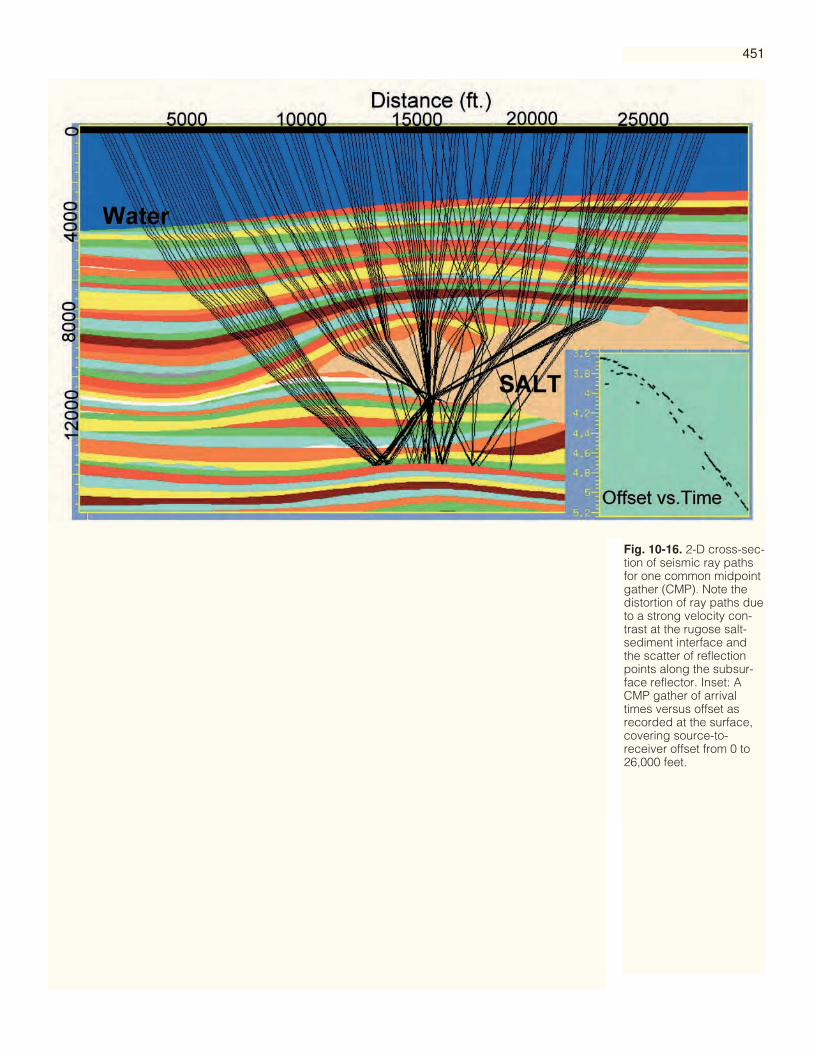
451

Fig. 10-16. 2-D cross-sec-tion of seismic ray pathsfor one common midpointgather (CMP). Note thedistortion of ray paths dueto a strong velocity con-trast at the rugose salt-sediment interface andthe scatter of reflectionpoints along the subsur-face reflector. Inset: ACMP gather of arrivaltimes versus offset asrecorded at the surface,covering source-to-receiver offset from 0 to26,000 feet.

horizontally. Depth imaging corrects for these variations whereas time imagingdoes not.

The benefit of the correction process inherent in depth imaging comes at a sub-stantial price. Significant interpreter effort is required build the interval velocitymodel and to update the velocity estimates while honoring geologic constraints.Also, much greater raw computational effort is required in depth migration, espe-cially in its 3-D and pre-stack manifestations.

Effective 3-D depth imaging of surface seismic data can be accomplished usingthe required elements of (1) appropriate acquisition coverage, (2) a robust andaccurate velocity representation of the subsurface, (3) 3-D ray tracing, (4) a depthmigration algorithm, and (5) an imaging expert. High-quality imaging results canbe obtained when each of these elements is also of high quality.

Even with optimal acquisition, depth imaging cannot overcome the shortcom-ings of blind spots in the subsurface. Although 3-D seismic coverage at the surfacemay be evenly distributed, substantial ray bending through lenses like rugose saltoften prevents parts of lower reflecting surfaces from being touched by penetratingenergy. As Figure 10-16 shows for a single surface CMP, there are gaps in the sub-salt illumination. Seismic processing alone cannot heal these gaps. Another effectcan occur when energy is not reflected back from the subsurface, but enters a layerof high contrast at what is known as the critical angle, where the wave energy isblocked. An example of this is shown in Figure 10-17; shots from outside a saltbody travel to the reflector, but only some of them return to the surface. With avalid model of the subsurface velocity, maps can be generated showing where andwhy this takes place based on counting the hits from ray tracing.

Another approach to understanding illumination variations is to model themusing full wavefields. This approach offers a volumetric view and understandingof lost data zones, and also calibrates troublesome variations in amplitude that donot represent geology. Figure 10-18 shows slices from a 3-D volume of zero-offset-wavefield depth migration amplitudes. Input to the migration consists of the simu-lated surface wavefield from a grid of point sources of equal strength distributedthroughout the earth model. The migration amplitudes have variations solely dueto variations of wave propagation in the earth, migration aperture, and migrationalgorithm, but are independent of reflector lithology and reflectivity. Therefore, thevalue of such maps for interpretation is to distinguish between incomplete illumi-nation effects and geology.

For our examples in the Gulf of Mexico, the velocity representation of the saltbodies and the enclosing sedimentary section require a robust representation of thesalt interface. The exact topology of the salt interface is critical to imaging success,as the ray bending there is so large. Even small errors in the local dip of the inter-face will fail to adequately place the subsurface energy. 3-D software is used tobuild, edit, and update the salt interfaces in great detail. Then, to complete the 3-Dvelocity model, the software is also required to handle additional velocity objects,velocity gradients, and gridded small-scale changes in the sedimentary section.Speed and accuracy are important in this process, but just as important is the abili-ty to communicate the model to geophysicists, geologists, managers and partners,so 3-D visualization software is employed.

The resulting velocity model is then used to calculate the ray paths that areneeded to illuminate the subsurface and correct for the bending of the reflectionenergy. The travel paths of the rays are also visualized to show where and why thesubsurface corrections take place. The ray calculations are then used by a migra-tion program to 3-D propagate the seismic energy recorded at the surface backthrough the earth model to illuminate the subsurface. Aspects of a good migrationalgorithm for depth imaging are speed, accuracy, low cost, and good noise han-dling characteristics.

452

Required Elementsof 3-D Depth

Imaging

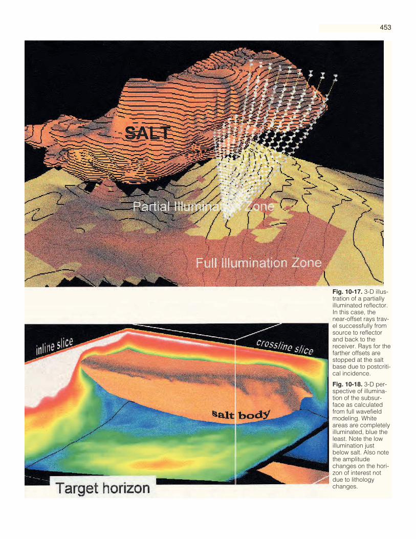
453

Fig. 10-17. 3-D illus-tration of a partiallyilluminated reflector.In this case, thenear-offset rays trav-el successfully fromsource to reflectorand back to thereceiver. Rays for thefarther offsets arestopped at the saltbase due to postcriti-cal incidence.

Fig. 10-18. 3-D per-spective of illumina-tion of the subsur-face as calculatedfrom full wavefieldmodeling. Whiteareas are completelyilluminated, blue theleast. Note the lowillumination justbelow salt. Also notethe amplitudechanges on the hori-zon of interest notdue to lithologychanges.

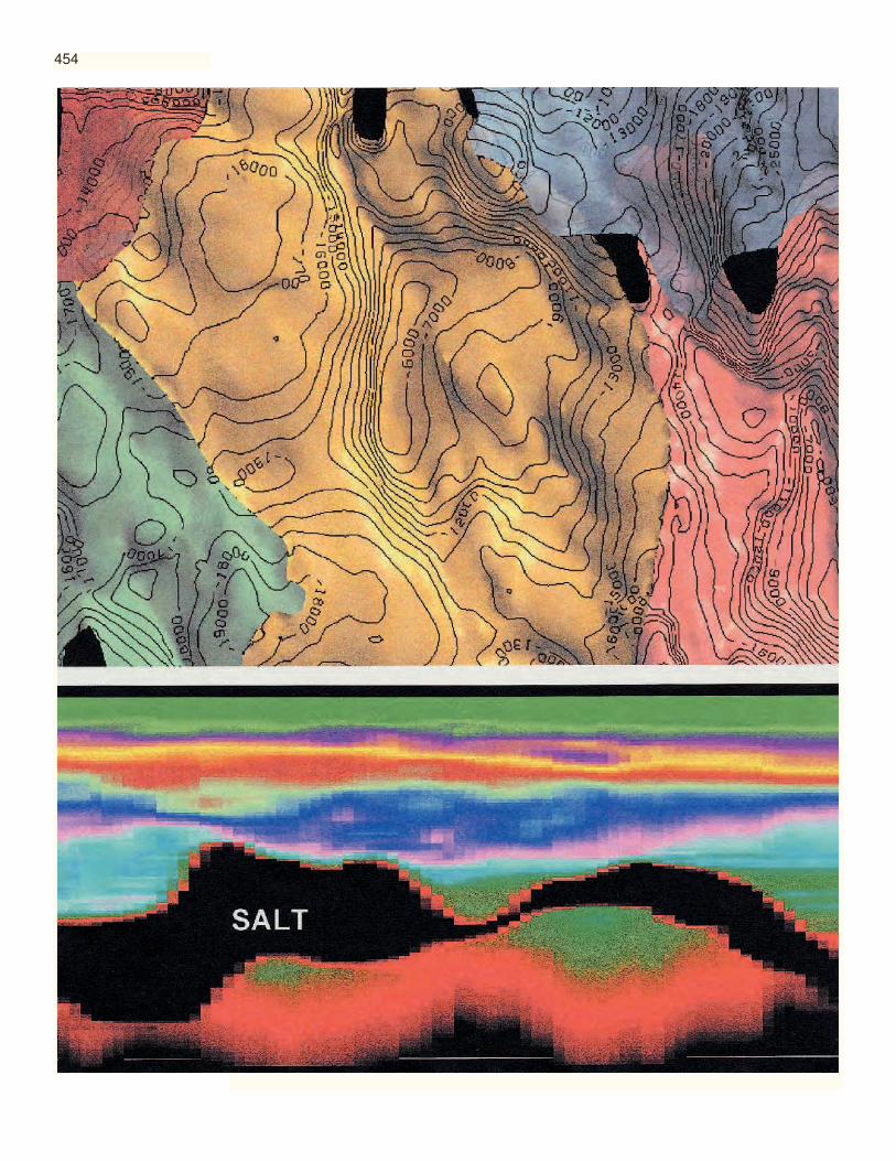
454

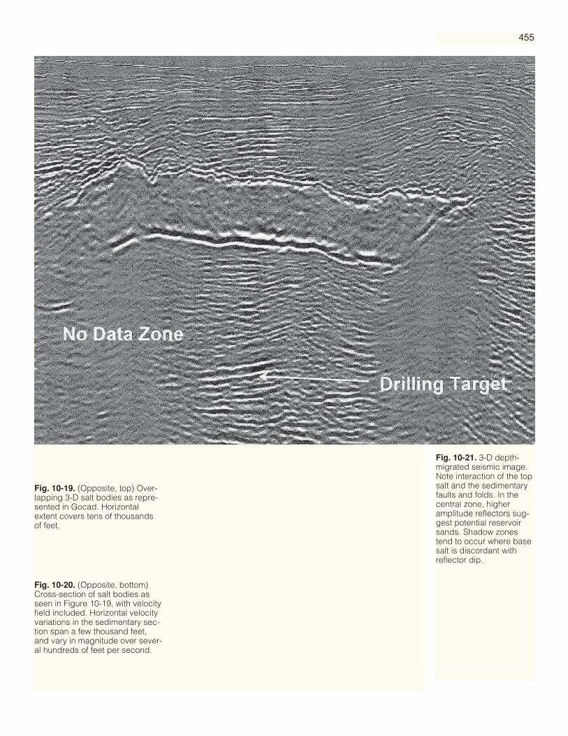
455

Fig. 10-21. 3-D depth-migrated seismic image.Note interaction of the topsalt and the sedimentaryfaults and folds. In thecentral zone, higheramplitude reflectors sug-gest potential reservoirsands. Shadow zonestend to occur where basesalt is discordant withreflector dip.

Fig. 10-19. (Opposite, top) Over-lapping 3-D salt bodies as repre-sented in Gocad. Horizontalextent covers tens of thousandsof feet.

Fig. 10-20. (Opposite, bottom)Cross-section of salt bodies asseen in Figure 10-19, with velocityfield included. Horizontal velocityvariations in the sedimentary sec-tion span a few thousand feet,and vary in magnitude over sever-al hundreds of feet per second.

Because the depth imaging process is employed in areas of high geological complexi-ty (from a velocity perspective), maximum information of the resulting images isgained when the experience of the depth imager is used in the interpretation. Signal,noise, shadow zones, depth uncertainty and position uncertainty can be validlyassessed when using the specific knowledge of how the image was formed and how itcan be modified.

Figures 10-19 to 10-21 illustrate some of the elements of the depth imaging process. Inone step, the tops of a series of overlapping salt bodies with high complexity (Figure 10-19) are represented with Gocad software. Notice that the surface contours in 3-D show agreat deal of structure at both the large and the fine scale. Both faulting and folding ofthe salt is represented faithfully to be sure that all of the ray bending can be accountedfor in seismic processing. An east-west cross-section (Figure 10-20) illustrates the sedi-mentary velocity surrounding these complex salt bodies. Variation in the velocity of thesurrounding sediments is a complex function of depth, geological age, deposition rate,compaction, lithology, pressure, and fluids. Accurate analysis and representation of thesediment velocity is important in imaging, as these changes determine the path of theseismic energy.

With adequately recorded seismic data and the appropriate velocity model, seismicimaging via high quality migration is then possible. An example of a depth-migratedsubsalt image from a similar but different area is shown in Figure 10-21. Several goodpoints can be made from this seismic image. Notice the complexity of the salt-sedimentinterface at the top. Faults and small-scale folds with 3-D geometry make the interfacehave local dips up to 45° immediately adjacent to planar salt sections.

Below the salt, prospective reflections (marked) can be seen that terminate both to theleft and right under non-illuminated shadow zones. Imaging may not be possible in theno-data locations as calculated from ray tracing. These shadow zones, apparently dueto postcritical ray blockage, are common when the dips of the reflector and the base saltbecome too discordant. Even so, the imaging below salt shows very encouraging eventsthat resemble the type of deepwater turbidite sands expected in a stratigraphic trappingposition. The consistent higher amplitude events lose reflectivity up the paleo-dip aswould be expected if they are deposited in a paleo-low. Utilizing the depth image, then,the prospective horizons under the salt were drilled. Sands were encountered in thezone of interest at the dip rates shown in the cross section.

Depth imaging is not only converting the time recordings to depth, but is also posi-tioning the data at the appropriate horizontal and vertical depth location. When com-paring the two approaches in a simple velocity area, they should give comparableresults. However, comparisons in complex velocity areas will be different. Inadequatetime imaging can be corrected through depth migration. Depth migration affects boththe structural and the amplitude information of the image.

An analogy of the impact of depth imaging over time imaging would be a similarcomparison of migrated time vs. unmigrated time data. An example would be whenunmigrated data can have large smooth anticlines that are really synclines whenmigrated! Depth imaging can sometimes have this much impact when the velocity ofthe earth is complicated and highly three-dimensional. Therefore, differences in migrat-ed time and migrated depth images will exist in areas of highly contrasting and varyingvelocity where the lens effects are greatest. The Gulf of Mexico subsalt play is a goodexample of just such an area.

As previously noted, depth imaging is not an improvement over time imaging whenan inaccurate (or even a moderately wrong) velocity model is used. Given the precisionof the migration algorithms to act as lens correctors, errors in the velocity model canpropagate odd-looking distortions that can be confused with geology. An example ofthis would be false faults or fold axes caused by inappropriate breaks in the velocitymodel. An additional caution should be noted. Noise in depth images appears differentfrom the same noise in time images, and in both cases the noise can be either similar to

456

3-D Post-stackDepth vs. 3-D Post-stack Time Imaging

or distinct from the signal. This becomes very important, when depth imaging isemployed in noisier than normal areas to bring out signal. When both the processingand the interpretation of the data are well connected, experience allows the avoidanceof pitfalls in velocity, noise and poor illumination zones.

As an example of post-stack time versus depth 3-D imaging, refer to Figures 10-22and 10-23. The difference between these sections is the migration velocity and themigration algorithms. In both cases, the input data are stacked in the time domain. Thegeology of the area is quite interesting. As observed in the time section of Figure 10-22,the shallow central anticline is underlain by a salt diapir. Deeper, the east dip extendsfrom the center to the edge of the data and a no-data zone extends under the salt fromthe center to the west.

Comparing the 3-D depth-migrated data (Figure 10-23), one sees significantly newinformation. First, a base of the salt can be seen in the depth-migrated data (A).Although the reflectivity of the base is not as stable as the top salt reflector, the base canbe mapped in 3-D. The reason one can now see this reflector is that depth migration ishonoring salt velocity and structure. It has correctly assembled the appropriate data,from both within and out of the plane of the section, into its coherent xyz location.

Deeper events in the depth image (B) imply a quite different structural history. Thepossibility of deep block faulting is suggested. This also sets the structural frameworkof the middle section (C) where dips have changed from monoclinal east to that of ahalf anticline. This is a significant change to the understanding of the structure. In addi-tion, the characteristics of the reflectors on the east flank are also different in the depthimage. Unfortunately, in the west flank of the subsalt, the noise characteristics have notimproved sufficiently to complete the subsalt picture. The attractive west dip segment(D) is a multiple! The subsalt section here probably cannot be improved using thestacked data as input to migration.

The high impact of depth migration is due to its application where the velocitymodel is complex. The salt velocity is about twice that of the sediments, and wavestraveling through salt rapidly deviate from trajectories appropriate to the time process-ing model of a layered earth. Additional differences are due to horizontally changingvelocity in the sedimentary section. Although lateral sedimentary velocity variation isoften modest, in some areas it can vary by up to a few thousand feet per second overseveral thousand feet, as it does below salt in Figure 10-23. Thus the impact of depthimaging is fairly small above salt but quite large in the deeper central section whereimaging is greatly affected by the rapid velocity contrasts of the geology.

As noted in the prior examples, depth migration is often applied in complex velocityenvironments where signal is desired in otherwise noisy areas. Because this is so, anunderstanding of the noise characteristics of these areas and how the imaging algo-rithm handles them becomes important.

Reflections of the subsurface that are correctly imaged are the signal we desire.Coherent energy that does not represent the earth reflectivity is a danger in our inter-pretation efforts. Mispositioned signal does not qualify as noise. Given the right veloci-ty model and acquisition sampling, this can be handled correctly. What we do need toclassify as coherent noise includes surface waves, refractions, mode conversions, multi-paths and multiples. These are most common in areas of complex structure and highvelocity contrasts, to the degree that the noise may be ten times stronger than the signalitself! The noise is not inherent in depth imaging, but depth imaging is more commonlyused in areas with these noise characteristics, thus we can expect depth images to com-monly contain noise.

Surface-generated coherent noise is common in land data, and especially trouble-some where the wavefield is strongly reflected or diffracted by surface objects (dunes,valleys, karst, etc.). Marine data also have surface-generated noise caused by sea bot-tom diffractors and waves trapped in near-surface low velocity zones. Surface generat-ed noise can sometimes be localized but often affects the entire seismic section.

457

Noise Characteristicsof Depth-imagedData

458

Fig. 10-22. 3-D post-stacktime migration. Comparewith Figure 10-23.

459

Fig. 10-23. 3-D post-stackdepth migration of sameinput data as for Figure10-22.

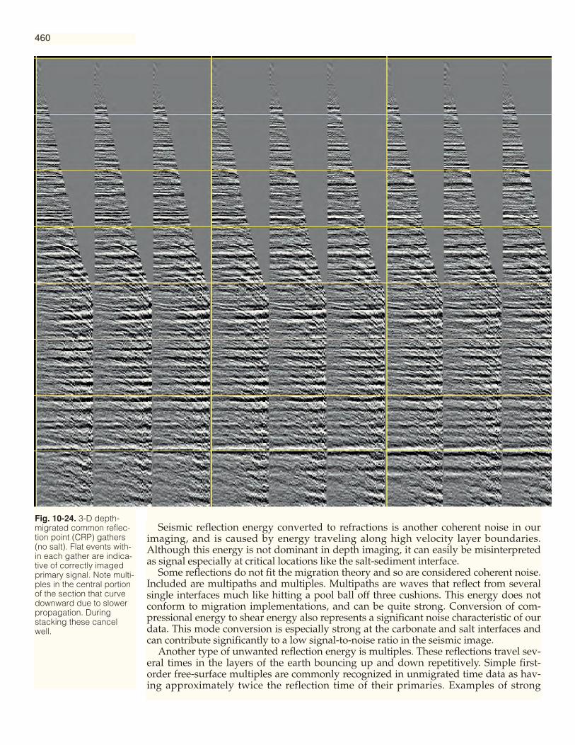
460

Fig. 10-24. 3-D depth-migrated common reflec-tion point (CRP) gathers(no salt). Flat events with-in each gather are indica-tive of correctly imagedprimary signal. Note multi-ples in the central portionof the section that curvedownward due to slowerpropagation. Duringstacking these cancelwell.

Seismic reflection energy converted to refractions is another coherent noise in ourimaging, and is caused by energy traveling along high velocity layer boundaries.Although this energy is not dominant in depth imaging, it can easily be misinterpretedas signal especially at critical locations like the salt-sediment interface.

Some reflections do not fit the migration theory and so are considered coherent noise.Included are multipaths and multiples. Multipaths are waves that reflect from severalsingle interfaces much like hitting a pool ball off three cushions. This energy does notconform to migration implementations, and can be quite strong. Conversion of com-pressional energy to shear energy also represents a significant noise characteristic of ourdata. This mode conversion is especially strong at the carbonate and salt interfaces andcan contribute significantly to a low signal-to-noise ratio in the seismic image.

Another type of unwanted reflection energy is multiples. These reflections travel sev-eral times in the layers of the earth bouncing up and down repetitively. Simple first-order free-surface multiples are commonly recognized in unmigrated time data as hav-ing approximately twice the reflection time of their primaries. Examples of strong

461

Fig. 10-25. 3-D depth-migrated CRP gatherswith intervening salt.Although stratigraphicallycontinuous with the near-by gathers of Figure 10-24, here flat subsalt signalis much weaker than thecurving coherent noise(multiples).

multiple generators are the air-water interface, ocean bottom, carbonate layers and salt.Complicating this situation are the shorter path, interbed multiples spawned among thebrighter reflectors. Although they are no stronger individually than free-surface multi-ples, the interbed population increases geometrically with the number of bright multi-ple generating interfaces, instead of proportionately as do the simple multiples. This isthe coherent noise challenge in subsalt imaging.

Figures 10-24 and 10-25 show 3-D depth-migrated traces of data before stacking. InFigure 10-24, the sedimentary signal is very strong, the velocity is well behaved, and thegathers are quite flat prior to stacking. With close inspection, some noise (multiples) can beseen that appears to be parabolic and turning down at the far offsets (to the right). In Fig-ure 10-25 a continuation of the same sedimentary section is represented subsalt, whereextensive mode conversions and multiples exist. Look hard and you will see the same flatreflectors are in these data, but they are about ten times weaker than the coherent noise.The subsalt seismic signal is weaker due to the conversion of much of the energy to noise.

462

All of the coherent noises described above exist in the time-imaged seismic sections,because they are a result of the seismic acquisition and the wavefield paths over whichthey travel. The depth imaging does not create the noise, but does distribute it different-ly than does time imaging. In the poor image portions of Figures 10-21 and 10-23, thesection is dominated by coherent noise. The energy there has a characteristic that isimportant to understand – it generally does not map in 3-D. This characteristic is mosteasily evaluated by using rapid 3-D movie views, and is very important in sorting outnoise from signal when they exist in equal strength.

Much of the noise characteristics of depth-imaged areas can be better understood byemploying seismic modeling. 3-D ray tracing can predict where the shadow zones are.The position and strength of multiples and mode conversions are also predictable.These predictions should be confirmed on the time-migrated data, and aid in the inter-pretation of time-imaged data. However, to understand noise in depth-imaged data,one must also account for the fact that the noise has been pushed though a depth migra-tion process that can scatter or collect noise in ways more complex than for time migra-tion.

As an example, Figure 10-26 illustrates a subsalt depth migration containing both sig-nal and noise. The velocity model used is one of a simple sedimentary velocity encasingsalt. However, the salt velocity layer is made infinitely thick below its top, so that thedepth migration is used to image and identify the base of the salt. Seismic ray tracemodeling of the multiple generated from the top of the salt plus an extra bounce in thewater layer shows complexity in 3-D. To match the depth-migrated wavefield image,the ray traced multiple was also “ray” depth migrated, and posted on the seismic cross-section in yellow. Where its overburden is simple, the multiple is very continuous andcan be wrongly identified as base salt. Where the 3-D ray paths are complex, the multi-ple incoherently migrates into alternately scattered and convergent zones. Having theray migrated multiple in this case allowed us to avoid a wrong interpretation of the saltbase and proceed with completing the salt velocity model and then imaging the subsaltsection.

Post-stack depth imaging uses the time stack as input to a depth migration. This is areasonable thing to do when the uncertainties of the velocity model are large, or cost is amajor issue. However, it is an imaging compromise. Stacking seismic data is the wrongthing to do in complex velocity areas, and depth migrating this simply moves thewrong data around without constructing the right image. Referring back to the inset inFigure 10-16, adding this erratically arriving signal along a hyperbola will produce afuzzy stack of the data, which can then be migrated. Pre-stack depth migration handleseach trace independently to create more precise image points in the subsurface.

It is important to note, for example, that the existence of an amplitude in stacked dataat a particular trace and time does not guarantee that it will find a place in the post-stack depth image. Assume that the stack amplitude comes mostly from the farther off-sets, while because of salt geometry the nearest offset ray experiences a quite differenttrajectory (or attenuates in a shadow zone). Then, because a post-stack migration algo-rithm maps data back along the zero-offset ray, a bias in its trajectory may misplace theentire stack amplitude or even carry it into oblivion.

With a good earth velocity model in areas of complex geometry and velocity, imagingaccuracy and precision are improved by pre-stack depth migration, which puts the sig-nal in the right location for each separate seismic trace and corrects for the lens effects oflarge velocity contrasts. Because the depth imaging areas are challenging, however, thesignal-to-noise ratio can vary greatly. The signal is placed in the correct CRP prior tostacking the traces, and gathers are more important in the interpretation process. Itbecomes important to recognize noise and improperly positioned signal on the gatherdata, and relate these back to the 3-D stacked volume to complete an effective interpre-tation.

Pre-stack DepthImaging

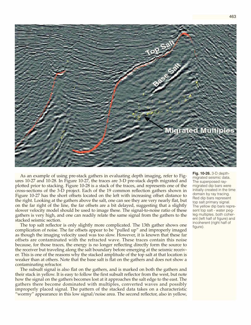
463

As an example of using pre-stack gathers in evaluating depth imaging, refer to Fig-ures 10-27 and 10-28. In Figure 10-27, the traces are 3-D pre-stack depth migrated andplotted prior to stacking. Figure 10-28 is a stack of the traces, and represents one of thecross-sections of the 3-D project. Each of the 19 common reflection gathers shown inFigure 10-27 has the short offsets located on the left with increasing offset distance tothe right. Looking at the gathers above the salt, one can see they are very nearly flat, buton the far right of the line, the far offsets are a bit delayed, suggesting that a slightlyslower velocity model should be used to image these. The signal-to-noise ratio of thesegathers is very high, and one can readily relate the same signal from the gathers to thestacked seismic section.

The top salt reflector is only slightly more complicated. The 13th gather shows onecomplication of noise. The far offsets appear to be “pulled up” and improperly imagedas though the imaging velocity used was too slow. However, it is known that these faroffsets are contaminated with the refracted wave. These traces contain this noisebecause, for those traces, the energy is no longer reflecting directly form the source tothe receiver but traveling along the salt boundary before emerging at the seismic receiv-er. This is one of the reasons why the stacked amplitude of the top salt at that location isweaker than at others. Note that the base salt is flat on the gathers and does not show acontaminating refractor.

The subsalt signal is also flat on the gathers, and is marked on both the gathers andtheir stack in yellow. It is easy to follow the first subsalt reflector from the west, but notehow the signal on the gathers becomes lost at it approaches the salt edge to the east. Thegathers there become dominated with multiples, converted waves and possiblyimproperly placed signal. The pattern of the stacked data takes on a characteristic“wormy” appearance in this low signal/noise area. The second reflector, also in yellow,

Fig. 10-26. 3-D depth-migrated seismic data.The superposed ray-migrated dip bars wereinitially created in the timedomain by ray tracing.Red dip bars representtop salt primary signal.The yellow dip bars repre-sent top salt - water peg-leg multiples, both coher-ent (left half of figure) andincoherent (right half offigure).

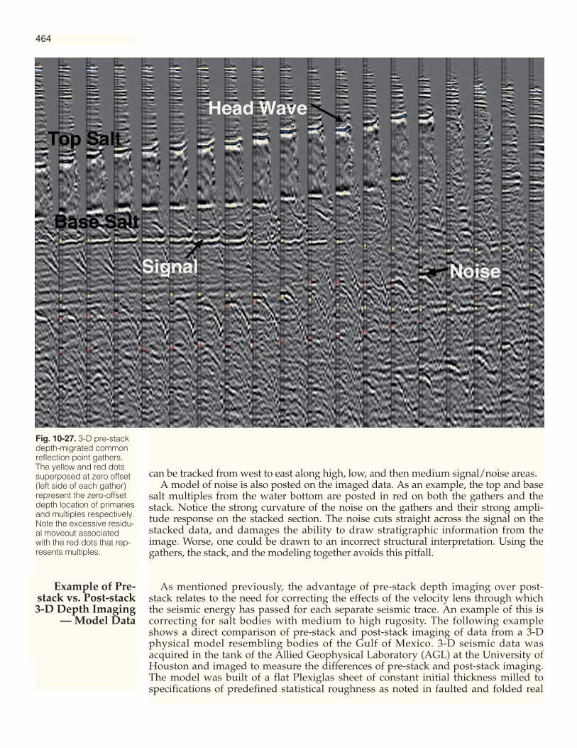
464

can be tracked from west to east along high, low, and then medium signal/noise areas.A model of noise is also posted on the imaged data. As an example, the top and base

salt multiples from the water bottom are posted in red on both the gathers and thestack. Notice the strong curvature of the noise on the gathers and their strong ampli-tude response on the stacked section. The noise cuts straight across the signal on thestacked data, and damages the ability to draw stratigraphic information from theimage. Worse, one could be drawn to an incorrect structural interpretation. Using thegathers, the stack, and the modeling together avoids this pitfall.

As mentioned previously, the advantage of pre-stack depth imaging over post-stack relates to the need for correcting the effects of the velocity lens through whichthe seismic energy has passed for each separate seismic trace. An example of this iscorrecting for salt bodies with medium to high rugosity. The following exampleshows a direct comparison of pre-stack and post-stack imaging of data from a 3-Dphysical model resembling bodies of the Gulf of Mexico. 3-D seismic data wasacquired in the tank of the Allied Geophysical Laboratory (AGL) at the University ofHouston and imaged to measure the differences of pre-stack and post-stack imaging.The model was built of a flat Plexiglas sheet of constant initial thickness milled tospecifications of predefined statistical roughness as noted in faulted and folded real

Fig. 10-27. 3-D pre-stackdepth-migrated commonreflection point gathers.The yellow and red dotssuperposed at zero offset(left side of each gather)represent the zero-offsetdepth location of primariesand multiples respectively.Note the excessive residu-al moveout associatedwith the red dots that rep-resents multiples.

Example of Pre-stack vs. Post-stack3-D Depth Imaging

— Model Data

465

Fig. 10-28. Stack of theCRP gathers of Figure 10-27. The trains of yellowand red dots exactly cor-respond to those in theprevious figure and aresimultaneously posted inboth views in practice.This assists the interpreterin discriminating betweenreflection signal (yellow)and coherent multiples(red). Note the wormyzone beneath the salt pinchout.

salt bodies exhibiting topological self-similarity (Figure 10-21). The Plexiglas sheetwas placed over a reflector model of a fault and two small anticlines, with four rodsinserted below to act as line diffractors (Figure 10-29). 3-D linear marine seismicacquisition was then performed over the model (AGL Model 93).

A digital representation of the model shows how the seismic energy is bent at thesalt-sediment interface (Figure 10-30). The top and base layers of the salt are represent-ed in a cut-away view to show the 3-D rays traveling through the salt. Notice that theCMP at the surface collects data from different locations on the reflector, so that a pre-stack process will be required to correct for this.

Seismic CMP gathers (Figure 10-31) show low signal/noise prior to stack, especiallyat the target horizon. Note that the physical model data has noise characteristics muchlike live data, in that it contains multiples and other noise like the mode conversionfrom P to S energy at the salt as noted. Although much of this noise is attenuated as aresult of the power of stacking in the time domain, nevertheless stacking before migra-tion degrades much of the signal, as we next illustrate.

Comparing an enlarged portion of the post-stack and pre-stack 3-D depth-migrateddata on a cross section of the model (Figures 10-32 and 10-33 respectively) shows whypre-stack imaging is preferred for stratigraphic quality imaging. The target horizon,anticline and fault are much clearer on the pre-stack data, and the lateral resolution of

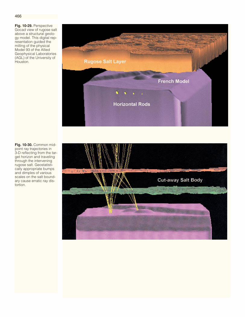
466

Fig. 10-29. PerspectiveGocad view of rugose saltabove a structural geolo-gy model. This digital rep-resentation guided themilling of the physicalModel 93 of the AlliedGeophysical Laboratories(AGL) of the University ofHouston.

Fig. 10-30. Common mid-point ray trajectories in 3-D reflecting from the tar-get horizon and travelingthrough the interveningrugose salt. Geostatisti-cally appropriate bumpsand dimples of variousscales on the salt bound-ary cause erratic ray dis-tortion.

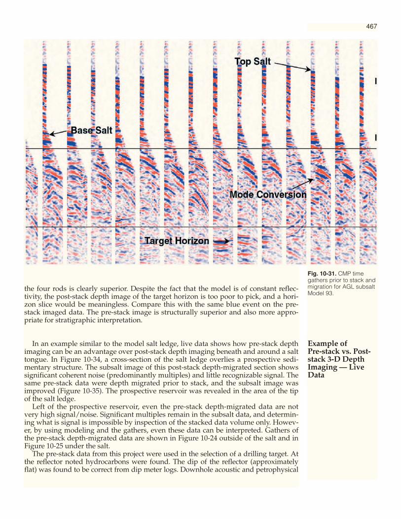
467

the four rods is clearly superior. Despite the fact that the model is of constant reflec-tivity, the post-stack depth image of the target horizon is too poor to pick, and a hori-zon slice would be meaningless. Compare this with the same blue event on the pre-stack imaged data. The pre-stack image is structurally superior and also more appro-priate for stratigraphic interpretation.

In an example similar to the model salt ledge, live data shows how pre-stack depthimaging can be an advantage over post-stack depth imaging beneath and around a salttongue. In Figure 10-34, a cross-section of the salt ledge overlies a prospective sedi-mentary structure. The subsalt image of this post-stack depth-migrated section showssignificant coherent noise (predominantly multiples) and little recognizable signal. Thesame pre-stack data were depth migrated prior to stack, and the subsalt image wasimproved (Figure 10-35). The prospective reservoir was revealed in the area of the tipof the salt ledge.

Left of the prospective reservoir, even the pre-stack depth-migrated data are notvery high signal/noise. Significant multiples remain in the subsalt data, and determin-ing what is signal is impossible by inspection of the stacked data volume only. Howev-er, by using modeling and the gathers, even these data can be interpreted. Gathers ofthe pre-stack depth-migrated data are shown in Figure 10-24 outside of the salt and inFigure 10-25 under the salt.

The pre-stack data from this project were used in the selection of a drilling target. Atthe reflector noted hydrocarbons were found. The dip of the reflector (approximatelyflat) was found to be correct from dip meter logs. Downhole acoustic and petrophysical

Fig. 10-31. CMP timegathers prior to stack andmigration for AGL subsaltModel 93.

Example of Pre-stack vs. Post-stack 3-D DepthImaging — LiveData

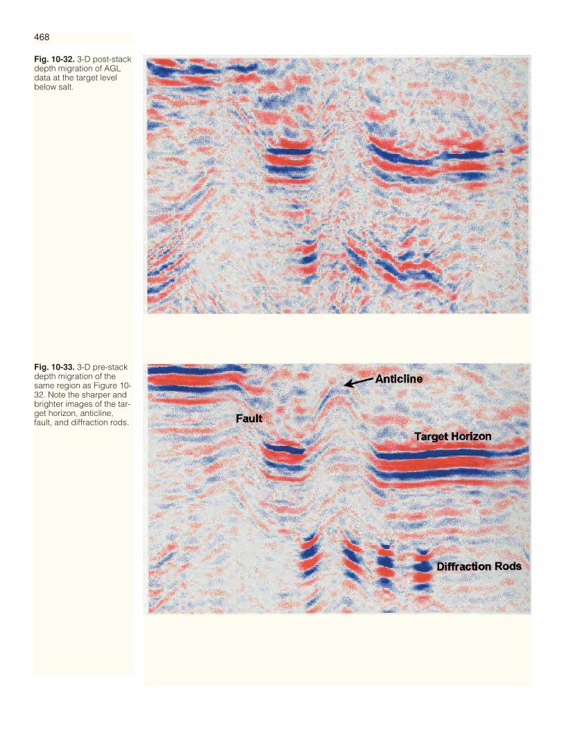
468

Fig. 10-32. 3-D post-stackdepth migration of AGLdata at the target levelbelow salt.

Fig. 10-33. 3-D pre-stackdepth migration of thesame region as Figure 10-32. Note the sharper andbrighter images of the tar-get horizon, anticline,fault, and diffraction rods.

469log data also show that the reflection characteristic of the reservoir is correct, as thehydrocarbons cause a bright spot relative to the surrounding section.

Interpretation of subsalt amplitude anomalies is an especially tricky practice. As theprior sections have noted, the pitfalls in trusting subsalt amplitudes are many. Incom-plete illumination, energy partitioning, coherent noise, improper velocity and inade-quate imaging algorithms can all contribute to poor subsalt signal response, anddestroy the quality of the imaging so that it falls well below what is needed for strati-graphic work.

But the good news is that understanding and accounting for these effects may alsoprovide satisfactory results. Figures 10-36 through 10-39 show a comparison of post-stack and pre-stack subsalt imaging where stratigraphic interpretation quality can beachieved. Figures 10-36 and 10-37 are post-stack and pre-stack sections, respectively,cutting through salt and an event of interest. The pre-stack image improves upon thepost-stack image throughout the cross-section, but nowhere is the interpretationalgain more pronounced than under and adjacent to the salt body. This is because thesubsalt data area was initially in need of the most improvement, which the pre-stackprocess delivered and the post-stack process could not. In particular, the events belowsalt are both sharper and more continuous on the pre-stack section. Of special note,because the pre-stack process does not rely on just the zero-offset ray to place ampli-tudes at depth but allows all ray trajectories to contribute to the image, there is muchless probability of subsalt event discontinuity. This is well illustrated by the disconti-nuity in the event of interest below the tip of salt. On the post-stack section the gap iswide and the interpretation suffers, but on the pre-stack section the gap is reduced toa narrow suture zone with less risk of misinterpretation.

As compelling as the cross-sectional comparison is, the dramatic improvement ofpre-stack over post-stack imaging is best seen in this case by comparing horizon sliceson the event of interest identified in the previous two figures. In Figure 10-38, thehorizon slice of post-stack 3-D depth-migrated data shows probable turbidite channeland overbank sands that are hard to follow under the salt ledge. Once under theledge, the event discontinuity first observed on the cross-section cuts a wide and inco-herent gash across the horizon, rendering interpretation risky. In Figure 10-39, thesame horizon sliced from the pre-stack image volume exhibits vastly greater geologiccontinuity and integrity of the channel and overbank system. The event continuity ismuch improved and can be followed with little risk.

In these examples, high quality 3-D pre-stack depth migration completes the neces-sary imaging process required to clarify the subsalt amplitudes. The horizon map isthen sufficient to define the limits of a potential reservoir for exploration and develop-ment purposes. A better understanding of the structural and stratigraphic context givesthe interpreter greater confidence in defining the geologic model and reducing risk.

Depth imaging is rapidly increasing in use in exploratory and development areas.For complex velocity and structural regimes, large differences can sometimes be seenfrom depth versus time imaging, as depth imaging can change the position, dip andamplitude of reflectors. Pre-stack depth imaging can also be advantageous over post-stack depth imaging under the right conditions. In either case, the noise characteristicsof the depth-imaged data are different from those of the time-imaged data, and mustbe taken into account during interpretation.

Depth imaging can be expensive due to the computational effort of getting the lenseffects corrected. An additional cost is incurred in getting a reasonable velocity modelto ensure imaging success. Another consideration is that the data are complex, andinterpretation is most valuable when the signal can be separated from the noise, anoth-er potentially costly procedure. Success in depth imaging can be achieved by using:

• A versatile 3-D earth model and robust model editor• Accurate velocity analysis and representation• Robust 3-D forward modeling of rays and waves• Visualization of ray tracing

Discussion

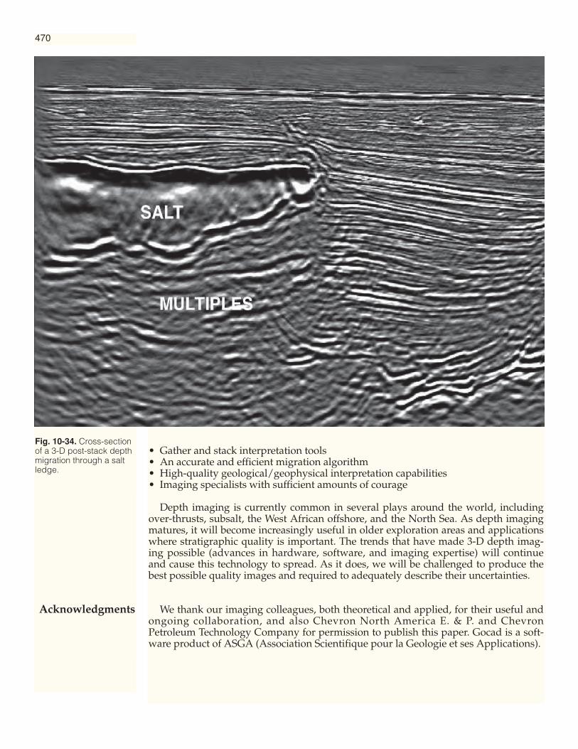
470

• Gather and stack interpretation tools• An accurate and efficient migration algorithm• High-quality geological/geophysical interpretation capabilities• Imaging specialists with sufficient amounts of courage

Depth imaging is currently common in several plays around the world, includingover-thrusts, subsalt, the West African offshore, and the North Sea. As depth imagingmatures, it will become increasingly useful in older exploration areas and applicationswhere stratigraphic quality is important. The trends that have made 3-D depth imag-ing possible (advances in hardware, software, and imaging expertise) will continueand cause this technology to spread. As it does, we will be challenged to produce thebest possible quality images and required to adequately describe their uncertainties.

We thank our imaging colleagues, both theoretical and applied, for their useful andongoing collaboration, and also Chevron North America E. & P. and ChevronPetroleum Technology Company for permission to publish this paper. Gocad is a soft-ware product of ASGA (Association Scientifique pour la Geologie et ses Applications).

Fig. 10-34. Cross-sectionof a 3-D post-stack depthmigration through a saltledge.

Acknowledgments

471

Fig. 10-35. Same as Fig-ure 10-34, but pre-stackdepth migrated.

472

Fig. 10-36. Cross-sectionof post-stack depth-migrated seismic dataalong line UT1 of Figure10-38. Note the wide sig-nal gap in the event ofinterest below the tip ofsalt.

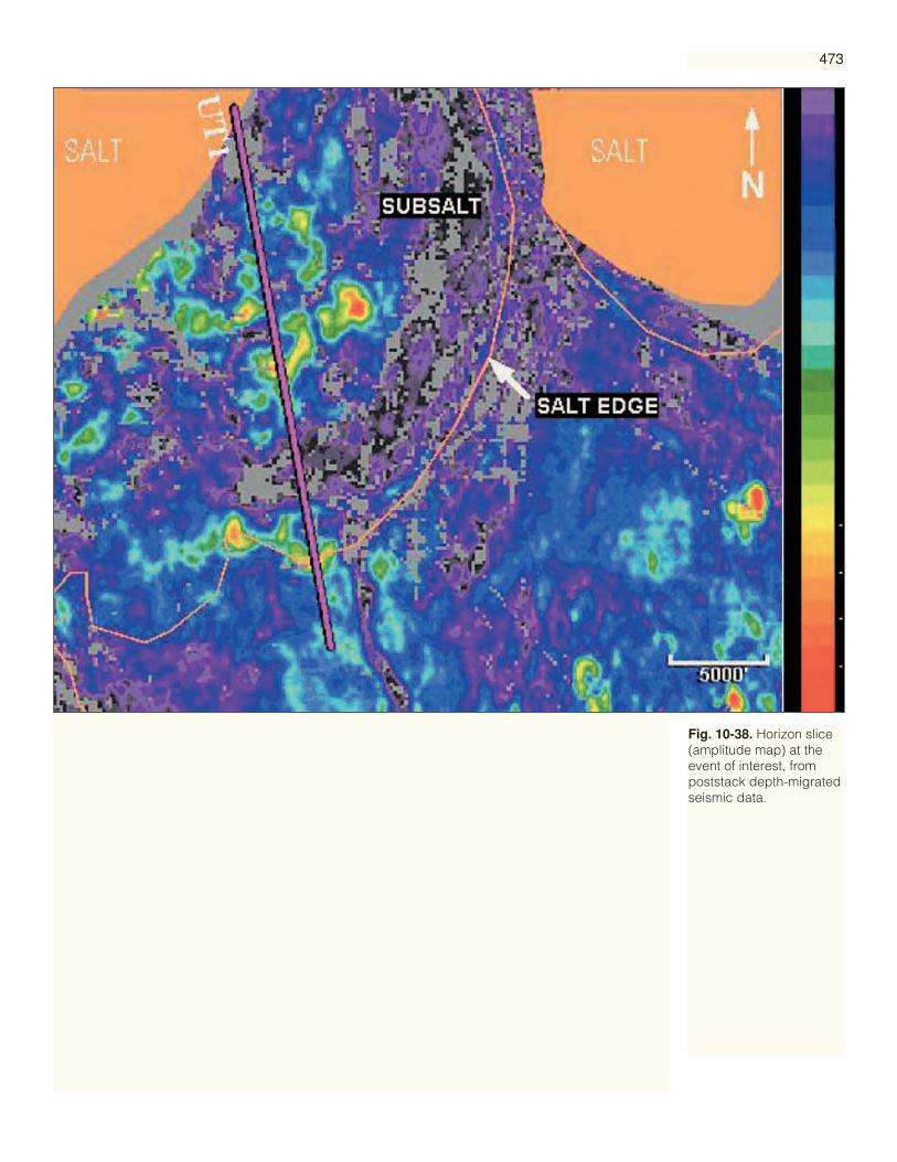
473

Fig. 10-38. Horizon slice(amplitude map) at theevent of interest, frompoststack depth-migratedseismic data.

474

Fig. 10-37. Cross-sectionof prestack depth-migrat-ed seismic data along lineUT1 of Figure 10-39. Thesignal gap in the event ofinterest below salt isreduced to a narrowsuture zone, and basesalt and other events aremuch better defined.

475

Fig. 10-39. Horizon slice(amplitude map) at theevent of interest, fromprestack depth-migratedseismic data. Note theimproved reflection conti-nuity crossing beneaththe salt edge.

477

Regional and Reconnaissance Use of 3-D Data

Three-D seismic coverage is now very extensive in both land and marine environ-ments, making practical the regional and reconnaissance use of 3-D data. This has ledto more exploration applications of 3-D surveys. More than 10 years ago there was atype of “Exploration 3-D” which involved widely spaced acquisition and interpola-tion in processing. Today all 3-D data are properly sampled and data acquisition isfast and highly efficient, particularly at sea.

Figures 11-1 through 11-4 show time slices from 1600 sq. km. of speculative 3-Dseismic coverage in the Gulf of Mexico, and this is only a small portion of the totaldata available. The four salt domes change with depth and the structural complexityincreases. Regional studies of salt tectonics are made possible with this kind of dis-play, and time slices are key in revealing the spatial patterns of faulting. Coherencedata displayed in time slices often provide improved visibility of fault patterns. Figure8-24 shows many faults clearly delineated in coherence over an area of 1400 sq. km.

Figure 11-5 covers 23,000 sq. km. offshore Louisiana and Texas, giving a thoroughlyregional view. The NE-SW Texas trend is clearly visible in the west, but over most ofthe time slice the E-W Louisiana trend is evident. Both these trends are consistent withsalt dome distribution, with fault orientation, and with gravity and magnetic data (J.S. Watkins, pers. comm., 2003). A prominent magnetic lineation is at the junction ofthe two trends, suggesting that the trends are caused by basement tectonics. A. W.Bally (1999) has long been promoting regional 3-D seismic coverage. He believes “thatregional tectonics will be completely recast as soon as regional 3-D seismic surveysbecome available to a larger community.”

Reconnaissance of 3-D data for amplitude anomalies can be accomplished quicklywith various carefully chosen displays. Figures 11-6 and 11-7 show a data volumefrom south Texas displayed with voxel transparency so that only the highest ampli-tudes are visible. The volume can be rotated and the best angle of view selected. Theexact amplitude threshold can also be adjusted as the interpreter’s understanding ofthe amplitude corresponding to gas develops. The data here are zero phase and nor-mal American polarity. This is why the gas bright spots appear red in Figure 11-6when we are looking down on them from the top, but blue in Figure 11-7 when we arelooking up at them from the bottom. We can here quickly review which bright spotshave been penetrated by wells and which have not.

Extensive joining, splicing, and merging of 3-D surveys to give regional coveragehave been accomplished in many parts of the world. PGS Geophysical has been heavi-ly involved in three areas offshore northwest Europe. The Central North Sea MegaSurvey has merged more than 150 separate surveys onto a standard north-south grid.The time slice of Figure 11-8 shows 35,000 sq. km. of coverage, but eventually this

CHAPTER ELEVEN

Text continued on page 494

Fig

. 11-

1.Ti

me

slic

e at

100

0 m

s fr

om G

ulf o

fM

exic

o sp

ecul

ativ

e 3-

D s

urve

y. A

rea

cove

rs 1

600

sq. k

m. N

ote

seve

ral c

hann

el p

atte

rns.

(C

ourt

esy

Wes

tern

Geo

phy

sica

l, a

div

isio

n of

Bak

er H

ughe

s.)

478

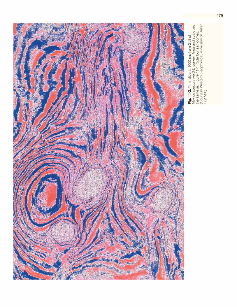
Fig

. 11-

2.Ti

me

slic

e at

200

0 m

s fr

om G

ulf o

fM

exic

o sp

ecul

ativ

e 3-

D s

urve

y. A

rea

and

sca

le a

reth

e sa

me

as F

igur

e 11

-1. N

ote

four

sal

t dom

es.

(Cou

rtes

y W

este

rn G

eop

hysi

cal,

a d

ivis

ion

of B

aker

Hug

hes.

)

479

Fig

. 11-

3.Ti

me

slic

e at

300

0 m

s fr

om G

ulf o

fM

exic

o sp

ecul

ativ

e 3-

D s

urve

y. A

rea

and

sca

le a

reth

e sa

me

as F

igur

e 11

-1. N

ote

sync

line

in n

orth

isno

w d

oub

le s

yncl

ine.

(C

ourt

esy

Wes

tern

Geo

phy

sica

l, a

div

isio

n of

Bak

er H

ughe

s.)

480

Fig

. 11-

4.Ti

me

slic

e at

400

0 m

s fr

om G

ulf o

fM

exic

o sp

ecul

ativ

e 3-

D s

urve

y. A

rea

and

sca

le a

reth

e sa

me

as F

igur

e 11

-1. N

ote

incr

ease

d a

rea

ofsa

lt an

d m

ore

faul

ting

. (C

ourt

esy

Wes

tern

Geo

phy

sica

l, a

div

isio

n of

Bak

er H

ughe

s.)

481

482

Fig. 11-5. Time slice at about 2 sec-onds from 3-D survey on the Gulf ofMexico shelf. The time slice measures356 km from east to west and coversan area of 23,000 sq. km. Note NE-SW trend in west and E-W trend ineast. (Courtesy Fairfield Industries.)

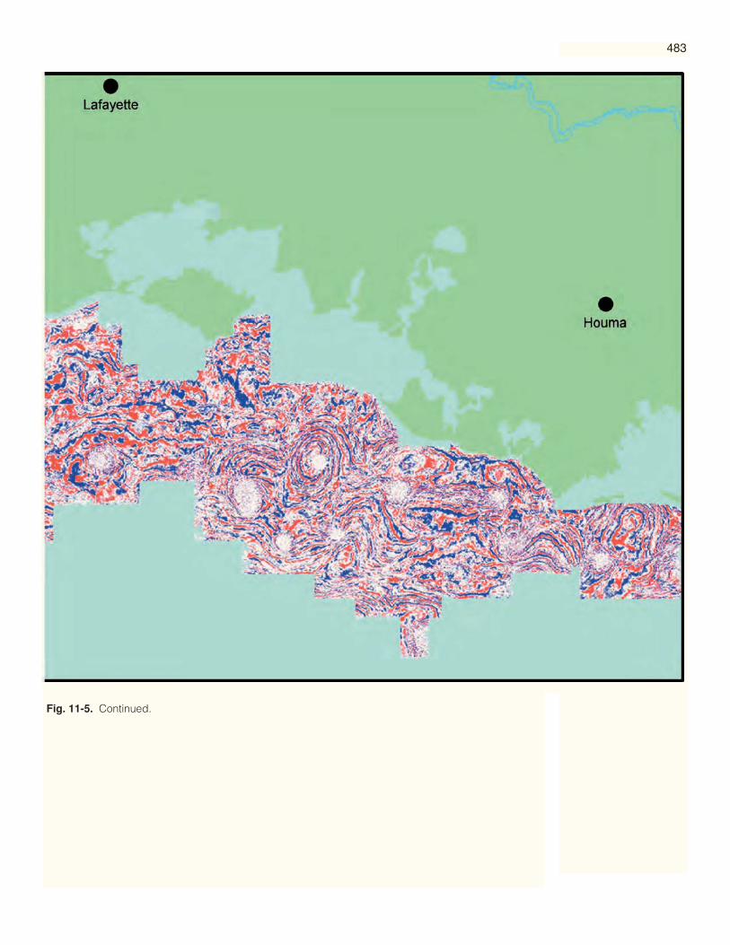
483

Fig. 11-5. Continued.

484

Fig

. 11-

6.V

olum

etric

vie

w o

f brig

ht s

pot

s in

the

Frio

For

mat

ion

of s

outh

Texa

s. T

he v

olum

e ha

s b

een

mad

e tr

ansp

aren

t exc

ept f

or th

e hi

ghe

st a

mp

li-tu

des

from

the

gas

acc

umul

atio

ns. T

he v

iew

is fr

om a

bov

e, s

o th

e re

d to

pg

as r

efle

ctio

ns a

re th

e p

rinci

pal

one

s se

en. T

he w

hite

line

s ar

e w

ells

. (C

our-

tesy

Ed

ge

Pet

role

um.)

485

Fig

. 11-

7.S

ame

as F

igur

e 11

-6 b

ut v

iew

ed fr

om b

elow

, so

the

blu

e b

ase

gas

refle

ctio

ns a

re th

e p

rinci

pal

one

s se

en. (

Cou

rtes

y E

dg

e P

etro

leum

.)

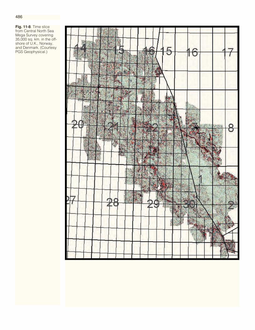
486

Fig. 11-8. Time slicefrom Central North SeaMega Survey covering35,000 sq. km. in the off-shore of U.K., Norway,and Denmark. (CourtesyPGS Geophysical.)

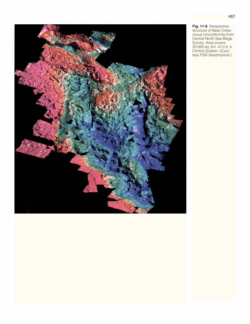
487

Fig. 11-9. Perspectivestructure of Base Creta-ceous Unconformity fromCentral North Sea MegaSurvey. Area covers20,000 sq. km. of U.K.’sCentral Graben. (Cour-tesy PGS Geophysical.)

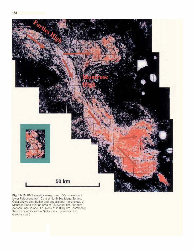
488

Fig. 11-10. RMS amplitude map over 100-ms window inlower Paleocene from Central North Sea Mega Survey.Color shows distribution and depositional morphology ofMaureen Sand over an area of 15,000 sq. km. For com-parison, inset is one U.K. block of 250 sq. km., commonlythe size of an individual 3-D survey. (Courtesy PGSGeophysical.)

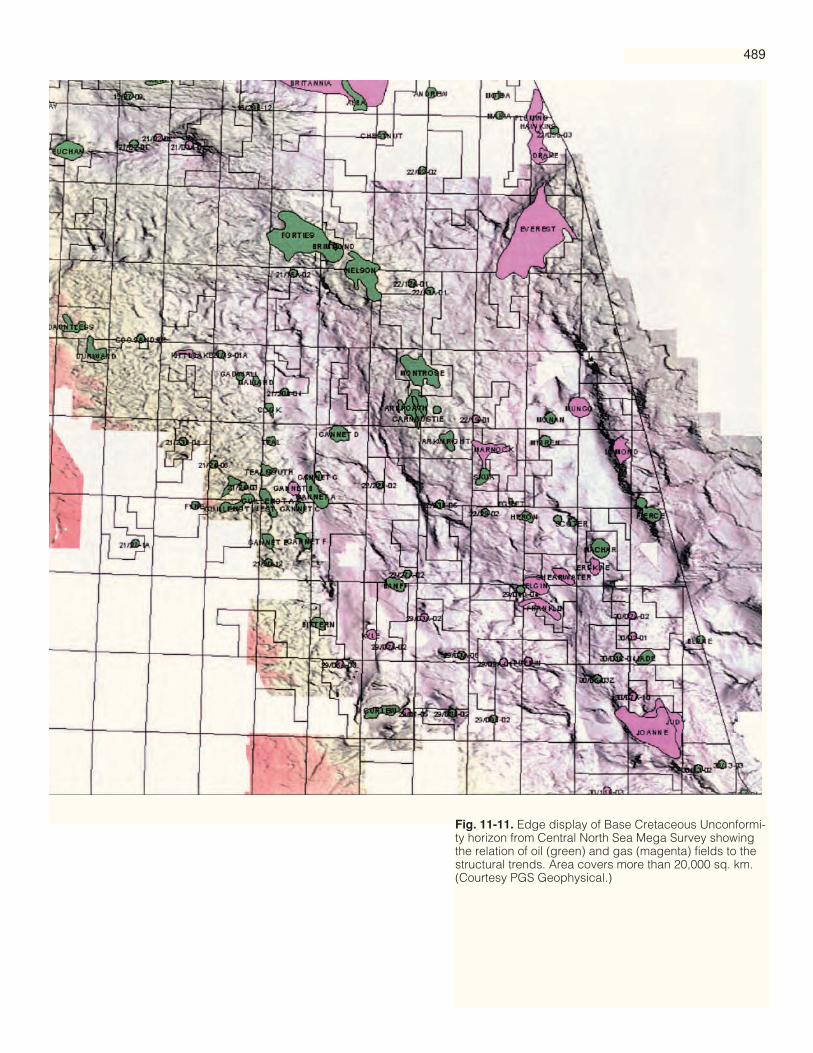
489

Fig. 11-11. Edge display of Base Cretaceous Unconformi-ty horizon from Central North Sea Mega Survey showingthe relation of oil (green) and gas (magenta) fields to thestructural trends. Area covers more than 20,000 sq. km.(Courtesy PGS Geophysical.)

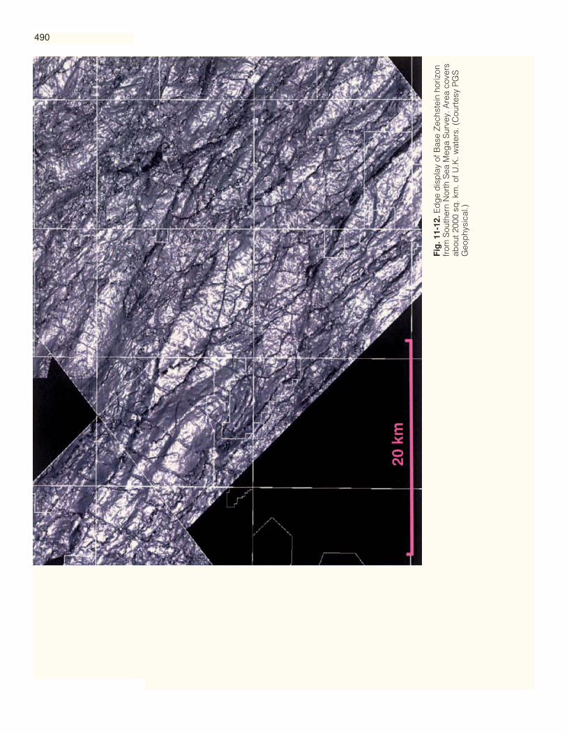
490

Fig

. 11-

12.E

dg

e d

isp

lay

of B

ase

Zec

hste

in h

oriz

onfr

om S

outh

ern

Nor

th S

ea M

ega

Sur

vey.

Are

a co

vers

abou

t 200

0 sq

. km

. of U

.K. w

ater

s. (

Cou

rtes

y P

GS

Geo

phy

sica

l.)

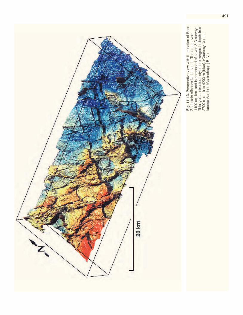
491

Fig

. 11-

13.P

ersp

ectiv

e vi

ew w

ith il

lum

inat

ion

of B

ase

Zec

hste

in o

ffsho

re N

ethe

rland

s. T

he a

rea

cove

rs11

00 s

q. k

m. a

nd is

com

pos

ed o

f sev

en 3

-D s

urve

ys.

This

typ

ical

str

uctu

ral s

tyle

her

e ra

nges

in d

epth

from

2700

m (

red

) to

420

0 m

(b

lue)

. (C

ourt

esy

Ned

er-

land

se A

ard

olie

Maa

tsch

app

ij B

. V.)

492

Fig. 11-14. Top Triassic structure from SouthernNorth Sea Mega Survey. Area covers 3000 sq. km.The patterns are caused by underlying mobile salt.(Courtesy PGS Geophysical.)

493

Fig. 11-15. Time structuremap with dip overlay fromOman. This mosaic madefrom eight multi-vintage 3-D land surveys has beenused for regional studies ofthe Cretaceous in southernOman. (CourtesyPetroleum DevelopmentOman LLC.)

total will be extended to 60,000 sq. km. (Edwards and Witney, 2002). Some of thesedata were used to generate the regional view of the Base Cretaceous Unconformity inFigure 11-9.

A wonderful demonstration of the value of regional coverage is shown in Figure11-10. Here, using the Top Chalk reflection as the reference horizon, a window from120 ms above to 20 ms above produced this amplitude map of the Maureen Sand. Thefan comes from the northwest, flows around the Forties and Montrose Highs andthen terminates in the deepest part of the Central Graben, where its forward progressis impeded by the Josephine High. For comparison in Figure 11-10, one U.K. block ofthe amplitude map is shown. This makes it clear that the nature and extent of thedeposition can only be understood by studying regional displays.

Figure 11-10 uses RMS (root-mean-square) amplitude over a 100-ms window. RMSamplitude is well suited to reconnaissance studies, as discussed in Chapter 4. Thereader is referred to the comparison between horizon and windowed amplitude inFigure 4-58.

Figure 11-11 is another interesting regional display from the Central North SeaMega Survey. The whole of the central North Sea may be viewed at once and the rela-tionship between Base Cretaceous structure and the existing fields can be studied eas-ily. The NW-SE structural trend apparently controls the oil and gas accumulations.

Figure 11-12 is from the Southern North Sea Mega Survey and shows part of thesouthern U.K. gas area. The orientation of the principal faults is northwest-southeast.This edge display clearly shows a secondary younger fault set running at right anglesto this primary trend, and the Mega Survey interpretation concludes that theseyounger faults are 50 km or more long. The structural style is evidently very similarto that across the median line in offshore Netherlands (Figure 11-13).

Figure 11-14 is from the Southern North Sea Mega Survey and shows the effect ofthe Zechstein salt movement at the Top Triassic level. The major disturbances trend-ing northwest-southeast (aligned with the yellow arrow) are caused by underlyingelongated salt walls. At the end of one of the walls faults can be seen radiating out-wards (the magenta arrow). Adjacent to another wall the faults are perpendicular (theblue arrow). The green arrow indicates a merge boundary between input 3-D surveys.

Figure 11-15 shows how the same joining of 3-D surveys has been accomplishedwith land data. Here eight surveys have facilitated the regional study of the Creta-ceous in southern Oman. Note various grabens oriented in a variety of directions.These eight surveys are part of a continuous swath of more than 40 surveys in thearea. Petroleum Development Oman, whose concession covers about half the country,now have so many 3-D surveys that they have introduced the 3-D MegaProject (Lig-tendag, 1999). Data are stored, manipulated, displayed and interpreted as MegaCellsmeasuring 10 � 10 km each, rather than as individual surveys. Each MegaCell is partof one of four MegaGrids, and a huge variety of regional displays is possible.

Bally, A. W., 1999, About geophysics, geology and regional hydrocarbon systems — adiscussion that contrasts the Gulf of Mexico with northeastern Venezuela: addressto Geophysical Society of Houston and Houston Geological Society.

Edwards, H., and J. Witney, 2002, The ‘mega survey’ route to understanding reservoirpotential: First Break, v. 20, p. 571-575.

Ligtendag, M. H. P., 1999, The 3-D MegaProject in Petroleum Development Oman: A3-D data management concept for seismic, workstation support and interpretation:The Leading Edge, v. 18, p. 330-337.

494

References

495

4-D Reservoir Monitoring

Time-lapse seismic in reservoir management is an important emerging technologyto help understand petroleum reservoirs and thus to produce more oil and gas fromthem (Jack, 1997). Four-D reservoir monitoring, an important part of the above,involves the study of two or more 3-D seismic surveys over the same reservoir in thehope of observing changes with time caused by petroleum production. The expectedchanges in the seismic data are generally small, so good data coupled with carefulprocessing and analysis are required.

Many projects to date have used legacy data, that is 3-D surveys which alreadyexist, acquired at different times over the same area or overlapping areas. Differencesin the positioning and acquisition of the seismic surveys are very problematical, sovery careful reprocessing is required. Even then legacy data will suffice only wherethere is a fairly large acoustic change in the reservoir and where the data are verygood (Figure 12-1). For lesser acoustic changes caused by production and for lessgood data areas, deliberately repeated surveys with conformable acquisition parame-ters will be needed. Some surveys have been and are being recorded by permanently-implanted receivers which greatly improves repeatability and which thus increasesthe detectability of subtle changes in the reservoir. Clearly this is easier to do on landthan at sea.

Between 30 and 40 projects are in progress worldwide but the commercial success-es reported to date are quite few, probably less than ten. With more deliberatelyrepeated surveys, permanently-implanted receivers and continuing technologyimprovements, more successes should be reported soon. In this chapter you will findsix case history examples of 4-D results; they are mentioned by name in Figure 12-1 intheir appropriate category. There is a further example reported as Case History 4 inChapter 9.

In fact 4-D seismic surveys to date have mostly studied secondary recovery. Figure12-2 shows the effect on acoustic impedance of several common production process-es. The effect of change in pressure within the reservoir is significant. In most casesthere is a change in fluid saturation and a change in pressure, so the effect on acous-tic impedance and thus amplitude is a combination of the two. We can reasonablyexpect to see a larger seismic change caused by production if the porosity of thereservoir rock is higher, if the rock is less consolidated, if it lies at a shallower depth,and if the exchanging fluids have a greater density contrast. Furthermore, becauseof seismic resolution a thicker reservoir will be a great benefit. Seismic traveltime isless affected by variations in positioning, acquisition or processing than seismicamplitude. So, if the reservoir changes affect traveltime, this may be a more robustindicator. Types of production that should be easier to monitor by 4-D seismic meth-ods include steam injection for heavy oil and tar, water flood for light oil, gas injec-tion, and oil production involving gas cap expansion.

CHAPTER TWELVE

Summary ofPrinciples

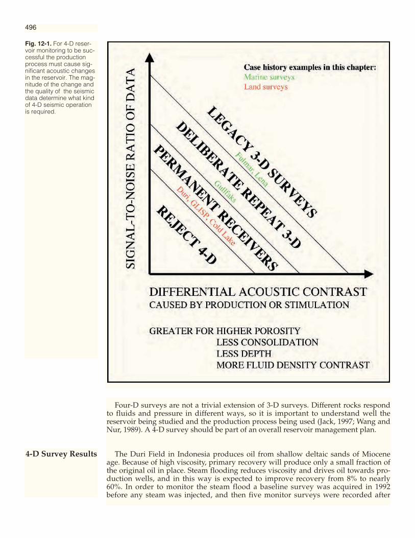
Four-D surveys are not a trivial extension of 3-D surveys. Different rocks respondto fluids and pressure in different ways, so it is important to understand well thereservoir being studied and the production process being used (Jack, 1997; Wang andNur, 1989). A 4-D survey should be part of an overall reservoir management plan.

The Duri Field in Indonesia produces oil from shallow deltaic sands of Mioceneage. Because of high viscosity, primary recovery will produce only a small fraction ofthe original oil in place. Steam flooding reduces viscosity and drives oil towards pro-duction wells, and in this way is expected to improve recovery from 8% to nearly60%. In order to monitor the steam flood a baseline survey was acquired in 1992before any steam was injected, and then five monitor surveys were recorded after

Fig. 12-1. For 4-D reser-voir monitoring to be suc-cessful the productionprocess must cause sig-nificant acoustic changesin the reservoir. The mag-nitude of the change andthe quality of the seismicdata determine what kindof 4-D seismic operationis required.

496

4-D Survey Results

steaming the reservoir for 2, 5, 9, 13 and 19 months (Lumley, 1995; Jenkins, Waite, andBee, 1997; Waite and Sigit, 1997). The pressure and heat of the steam causes progres-sive traveltime pull-ups and push-downs which can be seen on the sequence of verti-cal sections in Figure 12-3. The same progressive effects can be seen in Figure 12-4where on the time slices the effect of the steam can be seen as expanding circles, likerings from a pebble dropped into a pool of still water. On the two time slices to theright, after 13 and 19 months, the steam can be seen moving preferentially to thenorthwest (up in Figure 12-4). Figures 12-5, 12-6 and 12-7 are individual larger dis-plays after 0, 5 and 13 months.

In northern Alberta in Canada steam was injected into a heavy tar sand in order tomake it producible. Four 3-D surveys were used to monitor the steam effects. Anincrease in the temperature of the tar of 100 oC decreases its velocity by 50%. Thiswas observed by push-down of a deeper reflector and by increased amplitude in thetar sand section (Pullin, Matthews and Hirsche, 1987). The individual data volumeswere inverted into acoustic impedance and thence velocity. The velocity volumeswere then differenced and these difference volumes sliced. One such velocity differ-ence depth slice is shown in Figure 12-8, demonstrating in color the effect of the heatfrom injected steam.

Fig. 12-2. Effect onacoustic impedance, andthus amplitude, of com-mon production process-es for a high porosityunconsolidated sand-stone. Effects are smallerfor more consolidatedrocks and for less porousrocks. (After Wang andNur, 1989.)

497

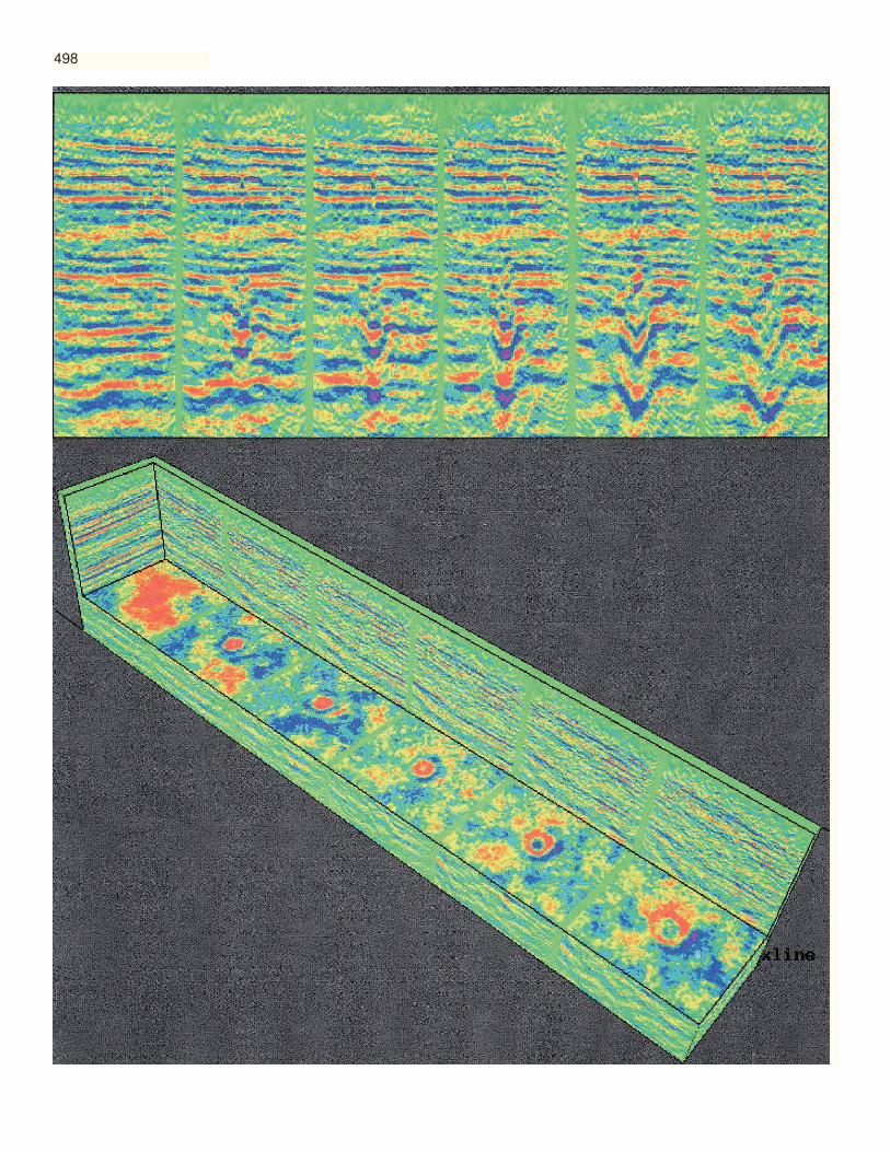
498

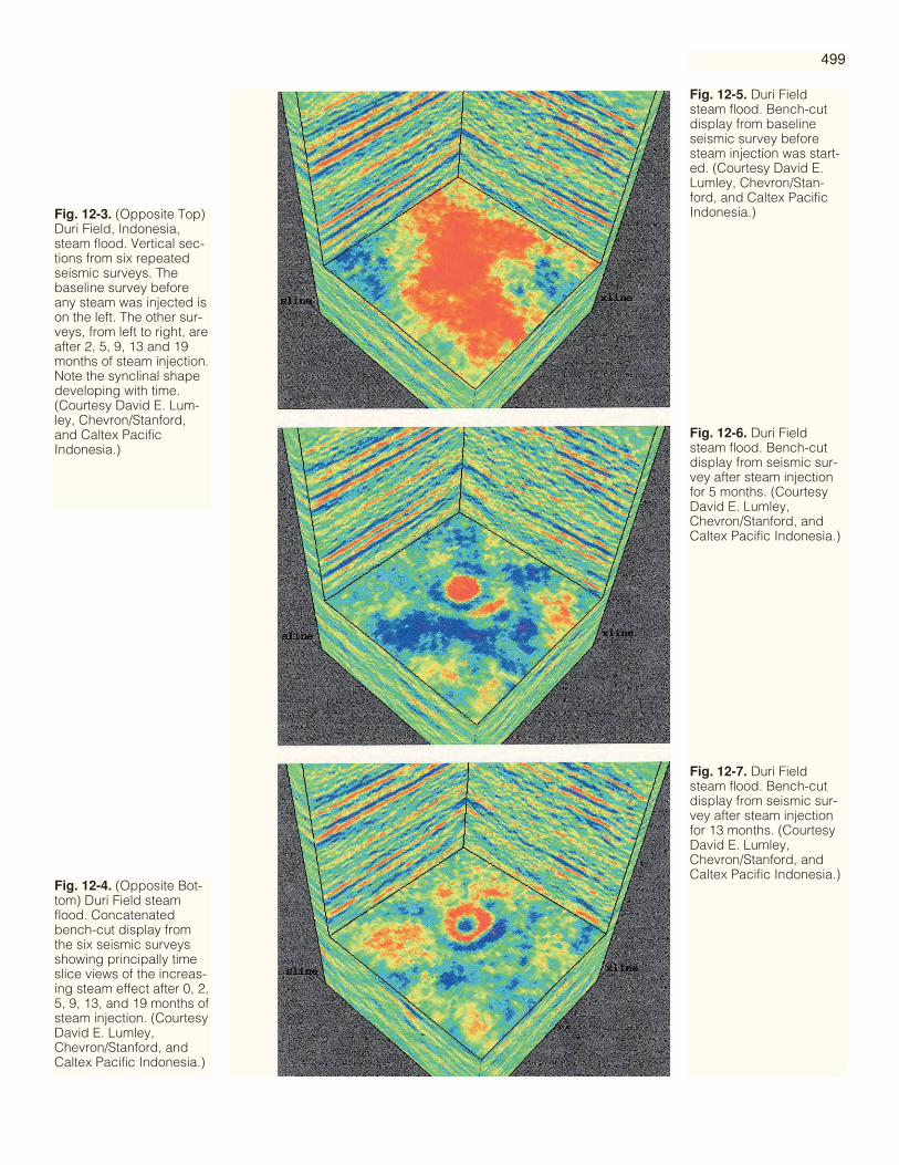
Fig. 12-3. (Opposite Top)Duri Field, Indonesia,steam flood. Vertical sec-tions from six repeatedseismic surveys. Thebaseline survey beforeany steam was injected ison the left. The other sur-veys, from left to right, areafter 2, 5, 9, 13 and 19months of steam injection.Note the synclinal shapedeveloping with time.(Courtesy David E. Lum-ley, Chevron/Stanford,and Caltex PacificIndonesia.)

Fig. 12-4. (Opposite Bot-tom) Duri Field steamflood. Concatenatedbench-cut display fromthe six seismic surveysshowing principally timeslice views of the increas-ing steam effect after 0, 2,5, 9, 13, and 19 months ofsteam injection. (CourtesyDavid E. Lumley,Chevron/Stanford, andCaltex Pacific Indonesia.)

499

Fig. 12-5. Duri Fieldsteam flood. Bench-cutdisplay from baselineseismic survey beforesteam injection was start-ed. (Courtesy David E.Lumley, Chevron/Stan-ford, and Caltex PacificIndonesia.)

Fig. 12-6. Duri Fieldsteam flood. Bench-cutdisplay from seismic sur-vey after steam injectionfor 5 months. (CourtesyDavid E. Lumley,Chevron/Stanford, andCaltex Pacific Indonesia.)

Fig. 12-7. Duri Fieldsteam flood. Bench-cutdisplay from seismic sur-vey after steam injectionfor 13 months. (CourtesyDavid E. Lumley,Chevron/Stanford, andCaltex Pacific Indonesia.)

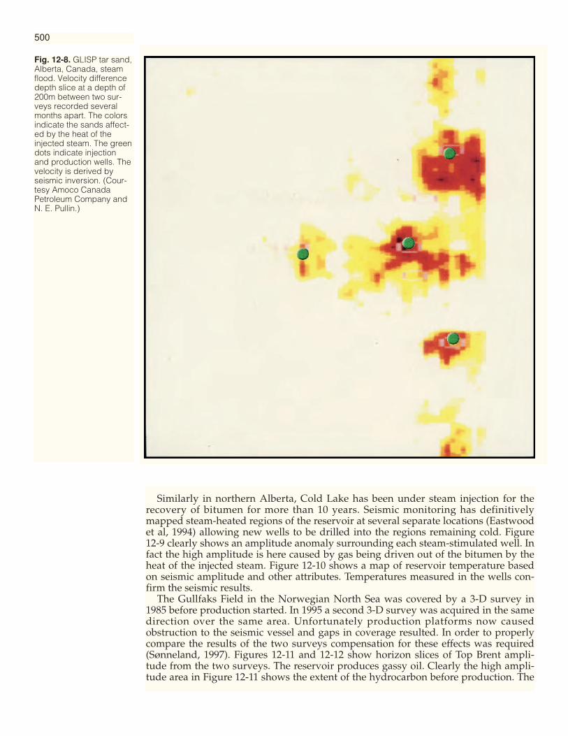
Similarly in northern Alberta, Cold Lake has been under steam injection for therecovery of bitumen for more than 10 years. Seismic monitoring has definitivelymapped steam-heated regions of the reservoir at several separate locations (Eastwoodet al, 1994) allowing new wells to be drilled into the regions remaining cold. Figure12-9 clearly shows an amplitude anomaly surrounding each steam-stimulated well. Infact the high amplitude is here caused by gas being driven out of the bitumen by theheat of the injected steam. Figure 12-10 shows a map of reservoir temperature basedon seismic amplitude and other attributes. Temperatures measured in the wells con-firm the seismic results.

The Gullfaks Field in the Norwegian North Sea was covered by a 3-D survey in1985 before production started. In 1995 a second 3-D survey was acquired in the samedirection over the same area. Unfortunately production platforms now causedobstruction to the seismic vessel and gaps in coverage resulted. In order to properlycompare the results of the two surveys compensation for these effects was required(Sønneland, 1997). Figures 12-11 and 12-12 show horizon slices of Top Brent ampli-tude from the two surveys. The reservoir produces gassy oil. Clearly the high ampli-tude area in Figure 12-11 shows the extent of the hydrocarbon before production. The

Fig. 12-8. GLISP tar sand,Alberta, Canada, steamflood. Velocity differencedepth slice at a depth of200m between two sur-veys recorded severalmonths apart. The colorsindicate the sands affect-ed by the heat of theinjected steam. The greendots indicate injectionand production wells. Thevelocity is derived byseismic inversion. (Cour-tesy Amoco CanadaPetroleum Company andN. E. Pullin.)

500

Fig. 12-9. Cold Lake,Alberta, Canada, steamflood. Seismic sectionthrough a row of steam-stimulated wells showingan amplitude anomalyassociated with each.(Courtesy Exxon Produc-tion Research Companyand Imperial Oil Limited.)

Fig. 12-10. Cold Lake,Alberta, Canada, steamflood. Seismically-derivedmap of hot (red) and cold(blue) reservoir based onmultiple seismic attributesincluding amplitude. Well-logged temperatures areannotated. (CourtesyExxon ProductionResearch Company andImperial Oil Limited.)

501

oil-water contact is rising by 13 m per year. Because of the residual saturation belowthe OWC the effect of production on the amplitude will be small. However, there areplaces in Figure 12-12 where the high amplitude seems to have moved back from theline of the initial OWC.

The Fulmar Field in the U.K. North Sea is covered by two legacy 3-D surveysrecorded in 1977 and 1992. There should be good chance of observing seismic differ-ences in this field because water is displacing light oil, the reservoir is a thick sand,and 10 years of production has taken place between the two surveys (Johnston et al,1998). Bright spots and flat spots clearly indicate a seismic expression of hydrocar-bons. Figure 12-13 shows horizon slices of Top Fulmar amplitude from the two sur-veys and they are different. At least some of the differences indicate the effects of pro-duction although there are also repeatability problems between the two legacysurveys. The two data sets were inverted into acoustic impedance; an average valuewas then calculated at each point from the top of the Fulmar Formation to the posi-tion of the original oil-water contact. Each of these was mapped and the differencebetween them produced Figure 12-14. Increases in impedance on the flanks of thestructure are interpreted as indications of water influx and pressure decline. Decreas-es in impedance on the crest are probably caused by injected gas.

The Lena Field in the Mississippi Canyon area of the Gulf of Mexico produces from

502

Fig. 12-11. Gullfaks Field,Norwegian North Sea,production of gassy oil.Horizon slice of Top Brentamplitude from 1985 3-Dsurvey recorded beforeproduction started. Highamplitudes tie with wellsthat found oil. OWC is at1947m. (Courtesy Statoil.)

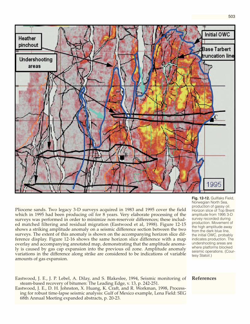
Pliocene sands. Two legacy 3-D surveys acquired in 1983 and 1995 cover the fieldwhich in 1995 had been producing oil for 8 years. Very elaborate processing of thesurveys was performed in order to minimize non-reservoir differences; these includ-ed matched filtering and residual migration (Eastwood et al, 1998). Figure 12-15shows a striking amplitude anomaly on a seismic difference section between the twosurveys. The extent of this anomaly is shown on the accompanying horizon slice dif-ference display. Figure 12-16 shows the same horizon slice difference with a mapoverlay and accompanying annotated map, demonstrating that the amplitude anoma-ly is caused by gas cap expansion into the previous oil zone. Amplitude anomalyvariations in the difference along strike are considered to be indications of variableamounts of gas expansion.

Eastwood, J. E., J. P. Lebel, A. Dilay, and S. Blakeslee, 1994, Seismic monitoring ofsteam-based recovery of bitumen: The Leading Edge, v. 13, p. 242-251.

Eastwood, J. E., D. H. Johnston, X. Huang, K. Craft, and R. Workman, 1998, Process-ing for robust time-lapse seismic analysis: Gulf of Mexico example, Lena Field: SEG68th Annual Meeting expanded abstracts, p. 20-23.

Fig. 12-12. Gullfaks Field,Norwegian North Sea,production of gassy oil.Horizon slice of Top Brentamplitude from 1995 3-Dsurvey recorded duringproduction. Movement ofthe high amplitude awayfrom the dark blue line,the initial OWC, probablyindicates production. Theundershooting areas arewhere platforms blockedseismic operations. (Cour-tesy Statoil.)

503

References

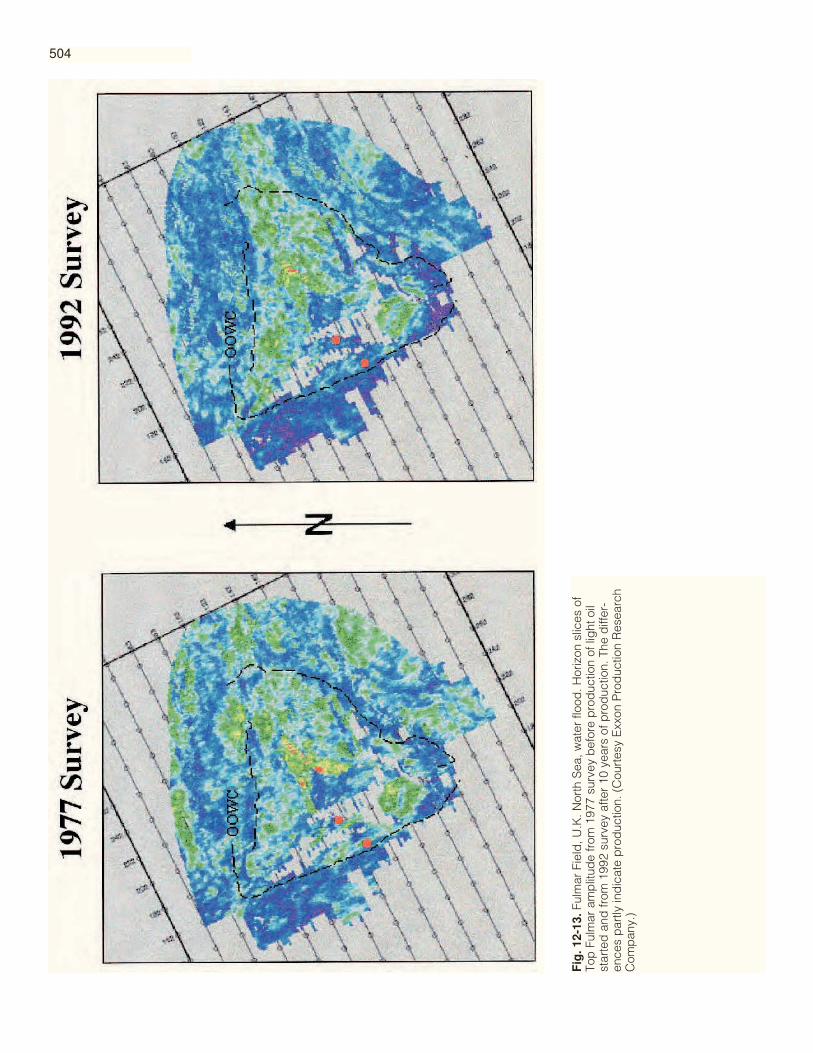
Fig

. 12-

13.F

ulm

ar F

ield

, U.K

. Nor

th S

ea, w

ater

floo

d. H

oriz

on s

lices

of

Top

Ful

mar

am

plit

ude

from

197

7 su

rvey

bef

ore

pro

duc

tion

of li

ght

oil

star

ted

and

from

199

2 su

rvey

afte

r 10

yea

rs o

f pro

duc

tion.

The

diff

er-

ence

s p

artly

ind

icat

e p

rod

uctio

n. (

Cou

rtes

y E

xxon

Pro

duc

tion

Res

earc

hC

omp

any.

)

504

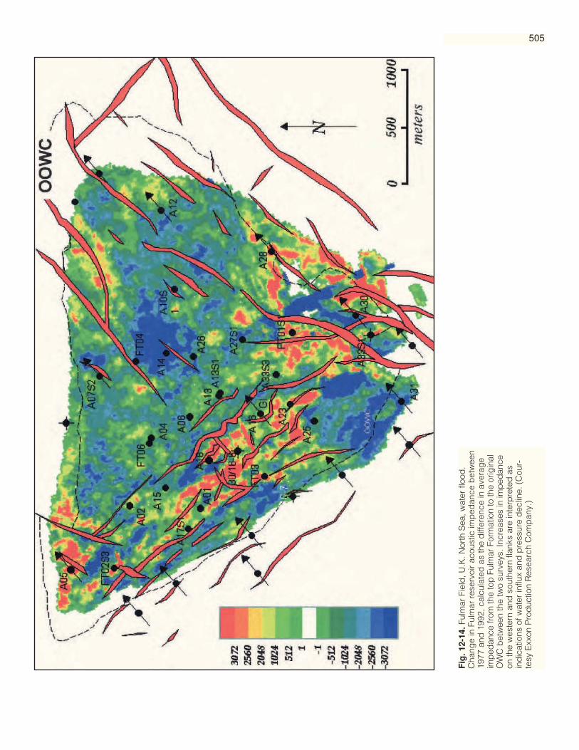
505

Fig

. 12-

14.F

ulm

ar F

ield

, U.K

. Nor

th S

ea, w

ater

floo

d.

Cha

nge

in F

ulm

ar r

eser

voir

acou

stic

imp

edan

ce b

etw

een

1977

and

199

2, c

alcu

late

d a

s th

e d

iffer

ence

in a

vera

ge

imp

edan

ce fr

om th

e to

p F

ulm

ar F

orm

atio

n to

the

orig

inal

OW

C b

etw

een

the

two

surv

eys.

Incr

ease

s in

imp

edan

ceon

the

wes

tern

and

sou

ther

n fla

nks

are

inte

rpre

ted

as

ind

icat

ions

of w

ater

influ

x an

d p

ress

ure

dec

line.

(C

our-

tesy

Exx

on P

rod

uctio

n R

esea

rch

Com

pan

y.)

Fig. 12-15. Lena Field,Gulf of Mexico, oil pro-duction and gas capexpansion. Seismic differ-ence section showinghigh amplitude caused bygas cap expansion in theB80 reservoir during 8years of production.Equivalent horizon sliceshowing the areal differ-ence in amplitudebetween the 1983 and1995 surveys. The yellowline shows the position ofthe section. (CourtesyExxon ProductionResearch Company andWestern Geophysical.)

506

Jack, I. G., 1997, Time-lapse seismic in reservoir management: Distinguished Instruc-tor Short Course notes, SEG.

Jenkins, S. D., M. W. Waite, and M. F. Bee, 1997, Time-lapse monitoring of the Duristeamflood: A pilot and case study: The Leading Edge, v. 16, p. 1267-1273.

Johnston, D. H., R. S. McKenny, J. Verbeek, and J. Almond, 1998, Time-lapse seismicanalysis of Fulmar Field: The Leading Edge, v. 17, p. 1420-1428.

Lumley, D. E., 1995, Seismic time-lapse monitoring of subsurface fluid flow: Ph. D.thesis, Stanford University, California, U.S.A.

Pullin, N. E., L. Matthews, and K. W. Hirsche, 1987, Techniques applied to obtain veryhigh resolution 3-D seismic imaging at an Athabasca tar sands thermal pilot: TheLeading Edge, v. 6, no. 12, p. 10-15.

Sønneland, L., H. H. Veire, B. Raymond, C. Signer, L. Pedersen, S. Ryan, and C. Say-ers, 1997, Seismic reservoir monitoring on Gullfaks: The Leading Edge, v. 16, p.1247-1252.

Waite, M. W., and R. Sigit, 1997, Seismic monitoring of the Duri steamflood: Applica-tion to reservoir management: The Leading Edge, v. 16, p. 1275-1278.

Wang, Z., and A. Nur, 1989, Seismic and acoustic velocities in reservoir rocks, SEG.

Fig. 12-16. Lena Field,Gulf of Mexico, oil pro-duction and gas capexpansion. Horizon slicedifference between 1983and 1995 surveys andcorresponding map,demonstrating that thehigh amplitude coincideswith the area of gas capexpansion. (CourtesyExxon ProductionResearch Company andWestern Geophysical.)

507

Considerations forOptimum 3-D SurveyDesign, Acquisition andProcessingMalcolm LansleyPGS Onshore, Inc.

The ideal 3-D seismic survey would have offset and azimuth distributions whichwere spatially very consistent. This means that the fold would have to be high. Costconsiderations, environmental concerns, topography, and the effects of surface infra-structure and other obstructions, usually result in the surface acquisition grid beingquite coarsely sampled and the offset and azimuth distributions being less than uni-form. These irregularities can cause difficulties in data processing and frequentlyresult in significant spatial variations in the amplitudes and phase of the final datavolume used for interpretation. Structural errors may also result. Because the varia-tions in trace attributes follow the variations in the surface geometry used for the dataacquisition, these effects cause an acquisition footprint or pattern of data acquisitionlineations. Special processing algorithms may be required to minimize these effects,but they are almost always present at some level on every data set. Prior to the inter-pretation of any data volume the interpreter should become familiar with the acquisi-tion geometry, the data processing flow, and potential artifacts that may have beenproduced. A careful balance between the spatial changes in trace attributes and thecost of the survey needs to be achieved during the design process.

There is also an important relationship between the spatial extent of the survey onthe surface and the subsurface area that must be correctly imaged. In the early stagesof survey design the necessary migration aperture is normally calculated and addedto the image area (Figure 1-12). Once the data acquisition geometry has beendesigned, the appropriate fold tapers are added to the outside of the migration aper-ture, and this then defines the surface extent of the survey. Cost pressures frequentlycause compromises to be made that result in the overall surface area being reduced.This leads to inadequate imaging of the target area that may result in the appearanceof false structures, particularly near the edges of the survey. Furthermore, after dataacquisition is completed, all of the data are sent to the data processing center and areused to create a migrated data volume. Upon completion of the data processing, theentire data volume normally is delivered to the interpreter and loaded onto the inter-pretation workstation. Only the central portion of this volume is correctly imaged, yetfrequently the entire data volume is used for interpretation, including the perimeterareas which have less than adequate fold, incomplete offset and azimuth distribu-tions, and are within the migration aperture.

General Issues

509APPENDIX A

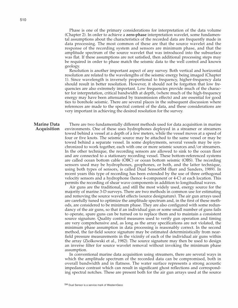
Phase is one of the primary considerations for interpretation of the data volume(Chapter 2). In order to achieve a zero-phase interpretation wavelet, some fundamen-tal assumptions about the characteristics of the recorded data are frequently made indata processing. The most common of these are that the source wavelet and theresponse of the recording system and sensors are minimum phase, and that theamplitude spectrum of the source wavelet that was introduced into the subsurfacewas flat. If these assumptions are not satisfied, then additional processing steps maybe required in order to phase match the seismic data to the well control and knowngeology.

Resolution is another important aspect of any survey. Both vertical and horizontalresolution are related to the wavelengths of the seismic energy being imaged (Chapter1). Since wavelength is inversely proportional to frequency, higher-frequency datashould result in better resolution. However, it should not be forgotten that low fre-quencies are also extremely important. Low frequencies provide much of the charac-ter for interpretation, critical bandwidth at depth, (where much of the high-frequencyenergy may have been attenuated by transmission effects) and are essential for goodties to borehole seismic. There are several places in the subsequent discussion wherereferences are made to the spectral content of the data, and these considerations arevery important in achieving the desired resolution for the survey.

There are two fundamentally different methods used for data acquisition in marineenvironments. One of these uses hydrophones deployed in a streamer or streamerstowed behind a vessel at a depth of a few meters, while the vessel moves at a speed offour or five knots. The seismic source may be attached to the same vessel or may betowed behind a separate vessel. In some deployments, several vessels may be syn-chronized to work together, each with one or more seismic sources and/or streamers.In the other technique, the recording sensors are allowed to sink to the ocean floorand are connected to a stationary recording vessel. These bottom-referenced systemsare called ocean bottom cable (OBC) or ocean bottom seismic (OBS). The recordingsensors used may be hydrophones, geophones, or both, and the latter technique,using both types of sensors, is called Dual SensorSM (Barr and Sanders, 1989). Inrecent years this type of recording has been extended by the use of three orthogonalvelocity sensors and a hydrophone (hence 4-component or 4-C) at each location. Thispermits the recording of shear wave components in addition to longitudinal waves.

Air guns are the traditional, and still the most widely used, energy source for themajority of marine 3-D surveys. There are two methods in common use for estimatingand removing the source wavelet effects (source designature). The air gun arrays usedare carefully tuned to optimize the amplitude spectrum and, in the first of these meth-ods, are considered to be minimum phase. They are also configured with some redun-dancy of the air guns, so that if an individual gun or some small number of guns failsto operate, spare guns can be turned on to replace them and to maintain a consistentsource signature. Quality control measures used to verify gun operation and timingare very comprehensive and, as long as the array specifications are not violated, theminimum phase assumption in data processing is reasonably correct. In the secondmethod, the far-field source signature may be estimated deterministically from near-field pressure measurements in the vicinity of each of the individual air guns withinthe array (Ziolkowski et al., 1982). The source signature may then be used to designan inverse filter for source wavelet removal without invoking the minimum phaseassumption.

In conventional marine data acquisition using streamers, there are several ways inwhich the amplitude spectrum of the recorded data can be compromised, both inoverall bandwidth and in flatness. The water surface represents a strong acousticimpedance contrast which can result in significant ghost reflections and correspond-ing spectral notches. These are present both for the air gun arrays used at the source

510

Marine DataAcquisition

SM Dual Sensor is a service mark of WesternGeco

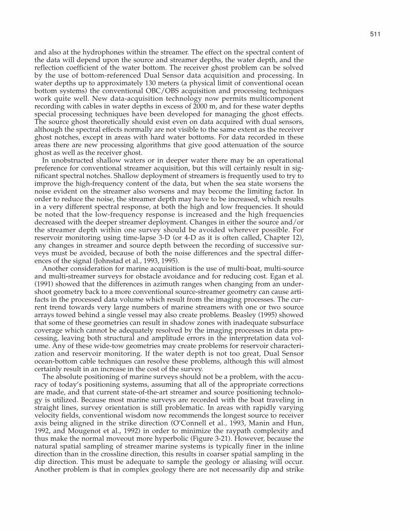
and also at the hydrophones within the streamer. The effect on the spectral content ofthe data will depend upon the source and streamer depths, the water depth, and thereflection coefficient of the water bottom. The receiver ghost problem can be solvedby the use of bottom-referenced Dual Sensor data acquisition and processing. Inwater depths up to approximately 130 meters (a physical limit of conventional oceanbottom systems) the conventional OBC/OBS acquisition and processing techniqueswork quite well. New data-acquisition technology now permits multicomponentrecording with cables in water depths in excess of 2000 m, and for these water depthsspecial processing techniques have been developed for managing the ghost effects.The source ghost theoretically should exist even on data acquired with dual sensors,although the spectral effects normally are not visible to the same extent as the receiverghost notches, except in areas with hard water bottoms. For data recorded in theseareas there are new processing algorithms that give good attenuation of the sourceghost as well as the receiver ghost.

In unobstructed shallow waters or in deeper water there may be an operationalpreference for conventional streamer acquisition, but this will certainly result in sig-nificant spectral notches. Shallow deployment of streamers is frequently used to try toimprove the high-frequency content of the data, but when the sea state worsens thenoise evident on the streamer also worsens and may become the limiting factor. Inorder to reduce the noise, the streamer depth may have to be increased, which resultsin a very different spectral response, at both the high and low frequencies. It shouldbe noted that the low-frequency response is increased and the high frequenciesdecreased with the deeper streamer deployment. Changes in either the source and/orthe streamer depth within one survey should be avoided wherever possible. Forreservoir monitoring using time-lapse 3-D (or 4-D as it is often called, Chapter 12),any changes in streamer and source depth between the recording of successive sur-veys must be avoided, because of both the noise differences and the spectral differ-ences of the signal (Johnstad et al., 1993, 1995).

Another consideration for marine acquisition is the use of multi-boat, multi-sourceand multi-streamer surveys for obstacle avoidance and for reducing cost. Egan et al.(1991) showed that the differences in azimuth ranges when changing from an under-shoot geometry back to a more conventional source-streamer geometry can cause arti-facts in the processed data volume which result from the imaging processes. The cur-rent trend towards very large numbers of marine streamers with one or two sourcearrays towed behind a single vessel may also create problems. Beasley (1995) showedthat some of these geometries can result in shadow zones with inadequate subsurfacecoverage which cannot be adequately resolved by the imaging processes in data pro-cessing, leaving both structural and amplitude errors in the interpretation data vol-ume. Any of these wide-tow geometries may create problems for reservoir characteri-zation and reservoir monitoring. If the water depth is not too great, Dual Sensorocean-bottom cable techniques can resolve these problems, although this will almostcertainly result in an increase in the cost of the survey.

The absolute positioning of marine surveys should not be a problem, with the accu-racy of today’s positioning systems, assuming that all of the appropriate correctionsare made, and that current state-of-the-art streamer and source positioning technolo-gy is utilized. Because most marine surveys are recorded with the boat traveling instraight lines, survey orientation is still problematic. In areas with rapidly varyingvelocity fields, conventional wisdom now recommends the longest source to receiveraxis being aligned in the strike direction (O’Connell et al., 1993, Manin and Hun,1992, and Mougenot et al., 1992) in order to minimize the raypath complexity andthus make the normal moveout more hyperbolic (Figure 3-21). However, because thenatural spatial sampling of streamer marine systems is typically finer in the inlinedirection than in the crossline direction, this results in coarser spatial sampling in thedip direction. This must be adequate to sample the geology or aliasing will occur.Another problem is that in complex geology there are not necessarily dip and strike

511

directions, and therefore any survey orientation may result in imaging difficulties inthe data processing stages.

For time-lapse 3-D surveys, Johnstad et al. (1993) showed that absolute positioningwas not a critical factor and that marine 3-D surveys could be adequately reposi-tioned to permit subtraction of the data sets to show fluid movements in an offshorereservoir. However, it has been shown that minimizing the differences in the pre-stackoffset and azimuth attributes between the base and monitor surveys is very importantin reducing the seismic differences caused by the data acquisition. One method devel-oped to achieve this is the use of steerable streamers to better match the streamerfeathering of the monitor survey to that of the base survey. Another methoddescribed by Widmaier et al. (2003) showed that repeating source locations, togetherwith an overlapped shooting configuration using additional outer streamers,improves azimuth preservation in 4-D acquisition. Also, by using a more closelyspaced streamer configuration, source-receiver azimuths can be repeated very accu-rately.

An additional note is in order for ocean bottom surveys. Once the ghost removalhas been accomplished, ocean bottom data are much closer in character to surveysrecorded on land than to streamer marine surveys. Thus an interpreter who is famil-iar with marine surveys may experience some difficulty with the character of oceanbottom surveys.

In data acquisition on land, there are many factors which affect our ability to recordbroad bandwidth data with a good signal-to-noise ratio. One of the more significantof these is the use of arrays. We reduce the amount of noise recorded by increasingthe size of the source or receiver arrays, but by doing so we may also attenuate thehigh-frequency signal. Significant energy absorption and loss of high frequencies alsooccurs in the unconsolidated weathering layers near the surface. If the geophones areburied, the effects of surface noises and the absorptive losses in the near-surface canbe reduced. Pullin et al. (1986) showed a dramatic improvement in signal-to-noiseratio, high-frequency signal content, and reduction of static shifts on data recordedwith a single geophone per recording channel buried 10 meters below the surface.Although the improvement was significant, geophones are rarely buried more than afew centimeters, except for reservoir monitoring studies. Here geophones orhydrophones are frequently deeply buried and left in place permanently so that theyare available for subsequent monitoring surveys. This gives the added advantage thatvariations in the water table and other near-surface effects are minimized on subse-quent time-lapse surveys.

When amplitude-versus-offset or amplitude-versus-offset-and-azimuth studies areplanned, the use of linear source and receiver arrays to attenuate both coherentsource-generated noise and random noise can be really problematical. This is becausethe arrays also attenuate the signal differently with offset and azimuth. Even if circu-lar arrays are used to eliminate the dependence on azimuth, there is still an offsetdependence. This signal attenuation is also frequency dependent, which makes a dataprocessing solution very difficult to achieve.

When explosives are used as a land source, we can normally make the data pro-cessing assumption that the source amplitude spectrum is flat and that the phasespectrum is minimum phase. With vibroseis, however, the amplitude and phasespectra of the recorded data are frequently misunderstood. In order to optimize thedata quality and minimize data processing difficulties, it is recommended that vibra-tors be set up such that the ground force signal of the vibrator is phase locked to thepilot sweep according to SEG recommendations (Geophysics, v. 59, p. 315-322) andthat the amplitude spectrum of the fundamental of the ground force signal is con-trolled to be flat. When this is done and the data are processed correctly, the resultantvibrator data will be reverse polarity to data recorded with explosives. No additional

512

Land DataAcquisition

phase matching filters should be required. The use of nonlinear sweeps (i.e., nonlin-ear frequency versus time functions) will require special treatment in data processingin order to handle the wavelet phase correctly.

The source and receiver geometry used for a survey is normally a compromisebetween competing factors: geologic objectives, environmental and other surface con-straints, and cost. Quite often it is possible to see effects on the finally processed datavolume which relate to the geometry used to acquire the data (footprint). Theseeffects will be reduced as trace density increases and offset and azimuth distributionsbecome more uniform. The footprint is usually more visible in the shallow sectionthan the deeper section because of the restricted offsets contributing to the stack andhence the lower fold. This problem can be reduced by acquisition of a survey withmore closely spaced source and receiver lines. Great care should be taken in the areasaround surface obstructions to minimize the variations in fold, offsets and azimuths.Reduced coverage often occurs because of rivers, lakes, villages, production facilitiesor unpermitted areas.

In data processing the objective is to maximize the useful signal bandwidth, to pro-vide the interpreter with a correct structural image, and to generate a wavelet ofknown, usually zero, phase and amplitudes that represent, as closely as possible, thespatial variations in the subsurface reflectivity. Because amplitudes are fundamentalin seismic analysis, correct management of amplitudes is very important in reservoircharacterization studies. Also, as changes in amplitudes are of critical importance inreservoir monitoring studies, correct amplitude processing is essential. When waveequation consistent processes are being considered, inadequacies in the sampling willresult in amplitude variations and phase errors, which are much more difficult todetect and correct.

An interpreter may be called upon to judge or suggest the applicability or effective-ness of an intermediate process prior to migration. This may be a dangerous step,even for the very experienced. It can be very difficult to evaluate the final result ofsome process on a shot or CMP gather before it has gone through the complete pro-cessing sequence including migration. It is always a good idea to request to see amigrated example both with and without the proposed process.

Great care should be taken in the initial steps of geometry assignment and datainitialization, because most subsequent processes depend upon the geometryassigned at this stage. On land surveys, special attention should be paid to areasaround surface obstructions to ensure that offset source and receiver locations are cor-rectly assigned. In marine surveys, particular attention should be paid to the binningtechnique used, especially in areas where the source-streamer axis is in the strikedirection. In this case, if the bin is made too wide in the crossline (and hence dip)direction, attenuation of high frequencies may result. Also, the use of overlappingbins should be used with care, because even though the fold of the resultant stackmay be more even, amplitudes will be smeared and will require special managementin multi-trace processes such as DMO.

A spatially invariant time function should be used for spherical divergence andinelastic attenuation compensation, and velocity-dependent algorithms should beavoided. Care should be taken to ensure that the amplitude recovery is based on the pri-mary reflectors and not on the energy of multiples and coherent source-generated noises.

Three-D surveys typically have high surface redundancies that make surface-con-sistent processes very powerful. Surface-consistent wavelet processing, amplitudecompensation, and static algorithms (both refraction and residual reflection) normallyprovide very stable solutions for most 3-D geometries.

In wavelet processing, it is important to ensure that the phase and amplitude spec-tra of the recorded data match the assumptions that are made in the deconvolutionprocess. Particular attention should be paid to the phase and amplitude spectra of

513

Data Processing

vibroseis data, especially when nonlinear sweeps are used or when surveys use morethan one energy source. Because the pilot sweep used for correlation is normally fil-tered with the same instrument recording filters as the data channels, the phaseeffects of the recording filters are removed and the amplitude effects are squared.Thus the observed filter effects are very different between the vibroseis and explosivedata. Also the field vibroseis correlation algorithms are normally zero-phase, andeither a model-based or analytically derived inverse filter may be necessary to con-vert the phase and amplitude spectra.

Surface-consistent amplitude compensation will correct for source and receivercoupling variations and any further data-dependent amplitude scaling or balancingshould be avoided.

The near-surface model used for long- to medium-wavelength static correction ofland surveys is frequently derived from refraction analysis of the first arrivals of theproduction data. In some cases, the acquisition geometry may lead to some instabilityof the solution, particularly in areas with low surface redundancy around obstruc-tions or near the edges of the survey. Rigorous quality control of the model is essen-tial to ensure the integrity of the final structural image. Static corrections, althoughtraditionally regarded as only being a problem for land data, are frequently necessaryon marine surveys also. Compensation is required for tidal and salinity effects andresidual statics may also be necessary to compensate for short spatial wavelengthvariations in the velocities and thicknesses of the near-water bottom layers.

Frequency-wavenumber (F-K) noise-attenuation algorithms work well for attenu-ating coherent source-generated noise (including multiples) as long as the data arewell sampled spatially. They are not very good, however, at preserving true ampli-tudes, and should therefore be avoided wherever possible. With wide azimuth sur-veys, the characteristics of the noises may vary considerably along different azimuthsbecause of different source and receiver array orientations. Alternative noise attenua-tion algorithms such as radon or F-X methods may be required to model and removethe noise. There are a wide variety of noise-attenuation algorithms available in theindustry, and the ability of any particular algorithm to correctly retain true amplitudeof the signal should be verified before its use.

Dip moveout (DMO) is used to compensate for the difference between the mid-point and the zero-offset point of data recorded with non-zero source to receiver off-sets. In accomplishing this, DMO produces true common reflection point gathers andeliminates the dip dependence of the stacking velocities. It is, however, very sensitiveto changes in both the azimuth and offset distributions of the data being processed.Even with perfectly regular geometry, the acquisition footprint caused by the normalspatial variations in offset distribution is frequently made worse with the applicationof DMO. Variations in fold and azimuths may also lead to strong amplitude changesand artifacts that are not truly representative of changes in the subsurface.Modifications to the DMO algorithms to compensate for these variations (e.g.,Beasley et al., 1992) are available and should be used to minimize these effects. Unlessprestack migration is going to be performed, DMO is a necessary step in the imagingprocess, even when the geologic dip is zero. However, it is frequently omitted fromthe processing sequence both as a cost-saving measure and also to eliminate anyproblems associated with its application on data that are inadequately sampled.

The amplitudes output from a conventional common mid-point (CMP) stack arenormally corrected for variations in fold by a recovery scalar which divides thesummed input trace amplitudes by the number of traces contributing to the stack. Ifthe energy being stacked is pure signal, then the output amplitudes should be correct.When the input traces are subject to varying amounts of random and coherent noise,this recovery scalar will not result in a true amplitude stack. Although alternativeschemes do exist to try to compensate for varying degrees of signal and randomnoise, the most consistent amplitudes will result from a survey that is recorded withas uniform fold as possible.

514

Another consideration for CMP stacking is the range of lateral velocity variationwithin the offset range being included in the stack. For the stack to be valid, any later-al velocity variations need to be sufficiently gradual such that the normal moveout forthe traces to be included in the stack is hyperbolic. Where the velocity field changestoo rapidly, and non-hyperbolic normal moveout is apparent, prestack depth migra-tion should be performed. An additional issue that has become more evident in recentyears is azimuthal velocity anisotropy. Modern land recording geometries havebecome much wider in azimuth and much better sampled in offset. With theimproved offset and azimuth sampling, it is often possible to observe different veloci-ties along different azimuths. Unless the velocity analysis and moveout applicationcomprehend these azimuthal variations, the CMP stack will be degraded.

Although significant improvement of signal continuity is frequently apparent afterthe application of post-stack random noise attenuation, some of the energy thatappears to be incoherent may, in fact, be diffraction energy that should be preservedfor the migration process. It is recommended that these algorithms be applied aftermigration.

In order to complete the imaging process and accurately focus the reflection energyat its correct spatial location and time (or depth), the process of migration is required.There are a number of different migration algorithms and methodologies that vary intheir ability to handle steep dips and also in their inherent positioning accuracy. Thereis a considerable amount of literature discussing the strengths and weaknesses of dif-ferent migration algorithms that is available elsewhere, so no discussion of algorithmdifferences will be made here. The accuracy of structural information from 3-D sur-veys is related not only to the accuracy of the migration algorithms, but also to theaccuracy of the velocity field that is used for the imaging. It should be emphasized,therefore, that great care must be exercised in building an accurate velocity model formigration, particularly in areas of complex geology. Deregowksi et al. (1997) showedhow small errors in the velocity field used for migration can dramatically reduce thelateral resolution in the final image.

The main decisions to be made with respect to migration are whether the migrationwill be performed prestack or post-stack, and whether a time or depth migrationalgorithm should be used. This selection is necessarily based on the complexity of thegeology, the data acquisition geometry and, in particular, the severity of the lateralvelocity gradients within the survey area (Figure 10-2). In a time-migration algorithm,the migration operator is spatially symmetric and therefore cannot correctly handlesignificant lateral velocity variations within the migration aperture. A depth-migra-tion operator is spatially variable and is designed to accurately position data accord-ing to the travel paths defined by the depth and velocity model provided to the algo-rithm. The importance of the correctness of this model cannot be overemphasized,and close involvement of the interpreter in the development of the model is essential.

The processing expert should consider whether a post-stack migration will providean accurate image, or whether a prestack migration will be necessary. As long as thenormal moveout within the CMP gathers is hyperbolic, a post-stack migration shouldprove satisfactory from a structural-interpretation point of view. If the lateral velocitygradients are significant within the range of prestack source to receiver offsets andazimuths, then non-hyperbolic normal moveout will be apparent on the prestackCMP gathers and pre-stack depth migration will be necessary to correctly migrate thedata. Survey orientation is sometimes carefully selected to minimize the effects ofrapid lateral velocity variations (e.g., streamer marine acquisition in the strike direc-tion), in order to permit the use of more economical post-stack migration algorithms.It should be noted, however, that because of an increasing requirement for prestackdata analysis, the increase in computing power, and the development of more accu-rate and faster migration algorithms, prestack migration is becoming more and morecommon. Frequently, a post-stack migration may be just an intermediate product.

If it is determined that a post-stack migration will be adequate, and if the lateral

515

velocity gradients are small compared with the required migration aperture, then apost-stack time migration should be satisfactory. If, however, the lateral velocitychanges are significant within the spatial extent of the migration aperture, then apost-stack depth migration is required.

For reservoir monitoring studies, the velocity model used for the imaging of suc-cessive surveys should be the same, or small differences in migration distance mightwell be interpreted as changes in the fluid content.

Barr, F.J., and J.I. Sanders, 1989, Attenuation of water-column reverberations usingpressure and velocity detectors in a water-bottom cable: 59th meeting, Society ofExploration Geophysicists, Expanded Abstracts, p. 653-656 .

Beasley, C. J., and R. Klotz, 1992, Equalization of DMO for irregular spatial sampling:54th Meeting, European Association of Exploration Geophysicists, ExpandedAbstracts, p. 232-233.

Beasley, C. J., and E. Mobley,1995, Spatial sampling characteristics of wide-towmarine acquisition: 57th Meeting, European Association of Geoscientists andEngineers, Expanded Abstracts.

Deregowski, S., R. Bloor, and C. Koeninger, 1997, Increasing lateral resolution: 59thMeeting, European Association of Geoscientists and Engineers Extended Abstracts.

Egan, M. S., K. Dingwall, and J. Kapoor, 1991, Shooting direction — a 3-D marine sur-vey design issue: The Leading Edge, v. 10, no. 11, p. 37-41.

Johnstad, S.E., R.C. Uden, and K.N.B. Dunlop, 1993, Seismic reservoir monitoringover the Oseberg Field: First Break, v. 11, no. 5, p.177-185.

Johnstad, S.E., R.H. Seymour, and P.J. Smith, 1995, Seismic reservoir monitoring overthe Oseberg Field during the period 1989-1992: First Break, v. 13, no. 5, p.169-183.

O’Connell, J.K., M. Kohli, and S. Amos, 1993, Bullwinkle — a unique 3-D experiment:Geophysics, v. 58, p. 167-176 .

Manin, M., and F. Hun, 1992, Comparison of seismic results after dip and strike acqui-sition: 54th Meeting, European Association of Exploration Geophysicists,Expanded Abstracts, p. 4-5.

Mougenot, J.M., E. Robein, I. Ravat, and A. Morash, 1992, Design of 3-D land acquisi-tion in a structurally complex environment: 54th Meeting, European Association ofExploration Geophysicists, Expanded Abstracts, p. 8-9.

Pullin, N. E., L. W. Matthews, and W. K. Hirsche, 1986, Techniques applled to obtainvery high-resolution 3-D seismic imaging at an Athabasca tar sands thermal pilot:56th Meeting, Society of Exploration Geophysicists, Expanded Abstracts, p. 494-497.

Widmaier, M., S. Hegna, F. Smit, and E. Tijdens, 2003. Azimuth preservation in marine4-D acquisition: 65th Meeting, European Association of Geoscientists andEngineers Extended Abstracts.

Ziolkowski, A., G. Parkes, L. Hatton, T. Haugland, 1982, The signature of an air gunarray: Computation from near-field measurements including interactions:Geophysics v. 47, p. 1413-1421.

516

References

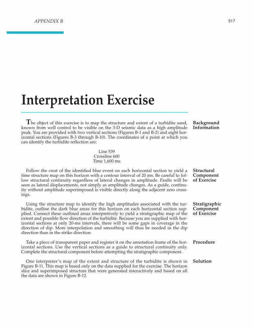
517

Interpretation ExerciseThe object of this exercise is to map the structure and extent of a turbidite sand,

known from well control to be visible on the 3-D seismic data as a high amplitudepeak. You are provided with two vertical sections (Figures B-1 and B-2) and eight hor-izontal sections (Figures B-3 through B-10). The coordinates of a point at which youcan identify the turbidite reflection are:

Line 539Crossline 600Time 1,600 ms

Follow the crest of the identified blue event on each horizontal section to yield atime structure map on this horizon with a contour interval of 20 ms. Be careful to fol-low structural continuity regardless of lateral changes in amplitude. Faults will beseen as lateral displacements, not simply as amplitude changes. As a guide, continu-ity without amplitude superimposed is visible directly along the adjacent zero cross-ings.

Using the structure map to identify the high amplitudes associated with the tur-bidite, outline the dark blue areas for this horizon on each horizontal section sup-plied. Connect these outlined areas interpretively to yield a stratigraphic map of theextent and possible flow direction of the turbidite. Because you are supplied with hor-izontal sections at only 20-ms intervals, there will be some gaps in coverage in thedirection of dip. More interpolation and smoothing will thus be needed in the dipdirection than in the strike direction.

Take a piece of transparent paper and register it on the annotation frame of the hor-izontal sections. Use the vertical sections as a guide to structural continuity only.Complete the structural component before attempting the stratigraphic component.

One interpreter’s map of the extent and structure of the turbidite is shown inFigure B-11. This map is based only on the data supplied for the exercise. The horizonslice and superimposed structure that were generated interactively and based on allthe data are shown in Figure B-12.

BackgroundInformation

Structural Componentof Exercise

StratigraphicComponentof Exercise

Procedure

Solution

APPENDIX B

518

Fig. B-1.

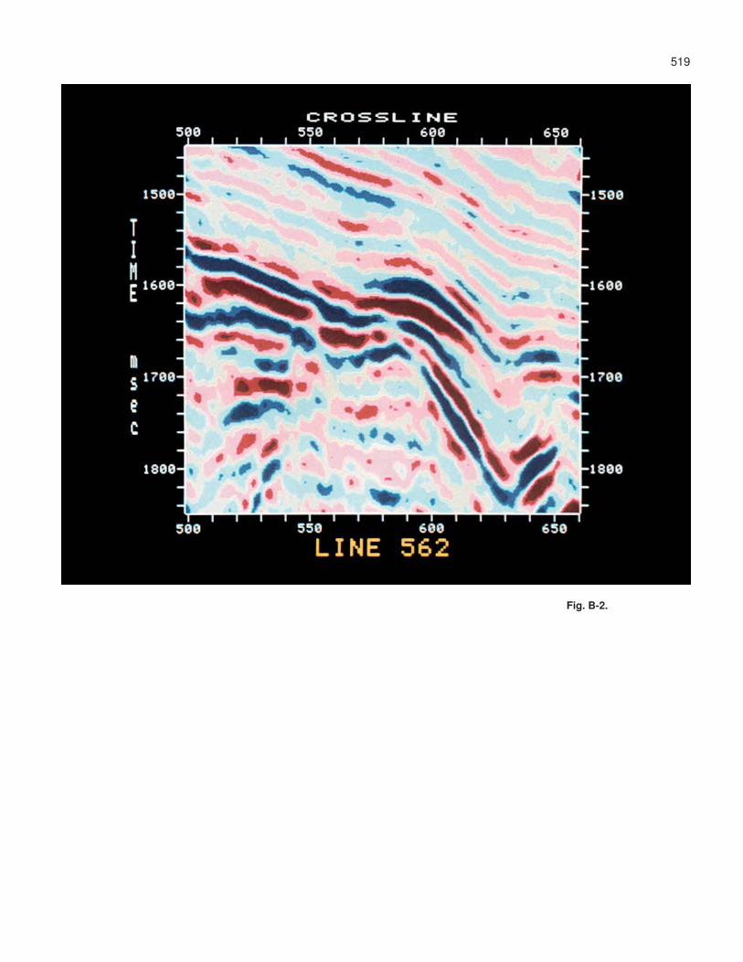
519

Fig. B-2.

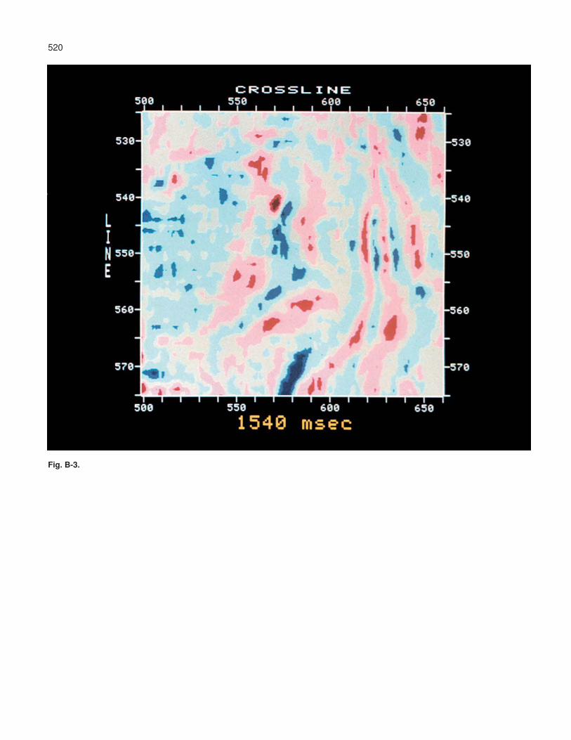
520

Fig. B-3.

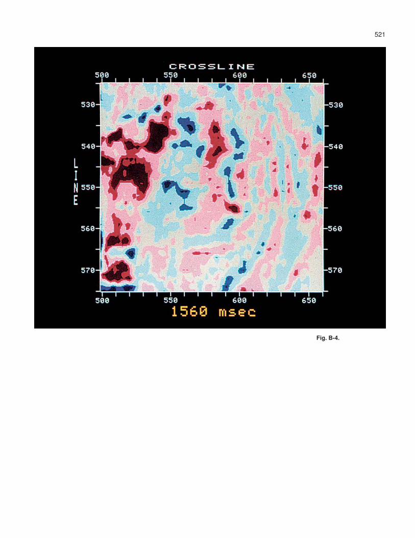
521

Fig. B-4.

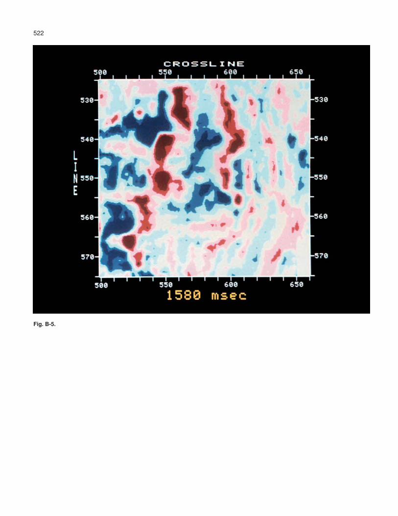
522

Fig. B-5.

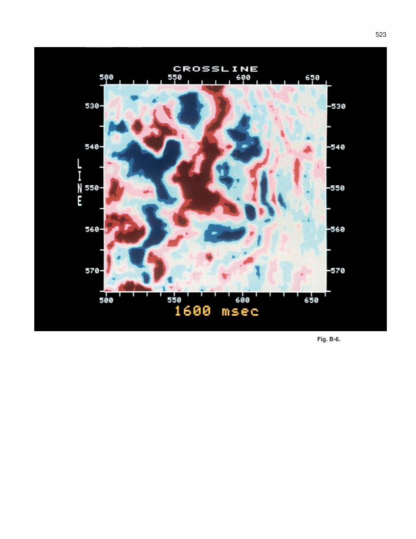
523

Fig. B-6.

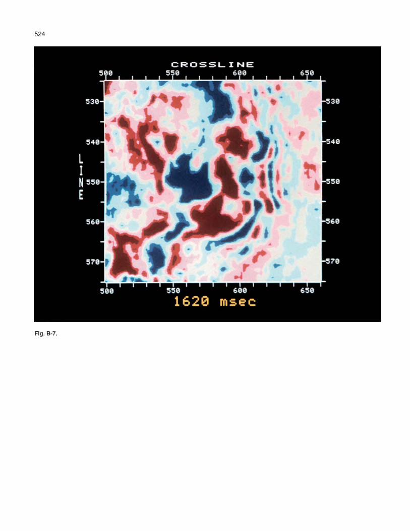
524

Fig. B-7.

525

Fig. B-8.

526

Fig. B-9.

527

Fig. B-10.

528

Fig. B-11.

529

Fig. B-12.

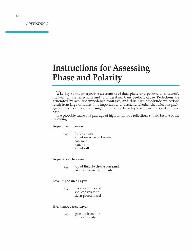
530

Instructions for Assessing Phase and Polarity

The key to the interpretive assessment of data phase and polarity is to identifyhigh-amplitude reflections and to understand their geologic cause. Reflections aregenerated by acoustic impedance contrasts, and thus high-amplitude reflectionsresult from large contrasts. It is important to understand whether the reflection pack-age studied is caused by a single interface or by a layer with interfaces at top andbase.

The probable cause of a package of high-amplitude reflections should be one of thefollowing:

Impedance Increase

e.g., fluid contacttop of massive carbonatebasementwater bottomtop of salt

Impedance Decrease

e.g., top of thick hydrocarbon sandbase of massive carbonate

Low-Impedance Layer

e.g., hydrocarbon sandshallow gas sandclean porous sand

High-Impedance Layer

e.g., igneous intrusionthin carbonate

APPENDIX C

Using general geologic knowledge of the area or using a well log, you should firstdecide which of these profiles is applicable. Then you should refer to the relevant dia-gram and compare the actual character of the high-amplitude reflections with thefour principal phase and polarity conditions. The data should be displayed with abalanced double-gradational color scheme using blue for positive amplitude and redfor negative amplitude. Select the diagrammatic character that best fits the data.Remember that ony primary lobes are shown in the diagrams; there will normally beflanking side lobes.

Phase and polarity circles are presented diagrammatically for a low-impedancelayer (Figure C-1), for a high-impedance layer (Figure C-2), and for an impedanceincrease (Figure C-3). An impedance decrease is not often used, so is not shown. Thefeature that is most reliable is the low-impedance layer. A second phase and polaritycircle using real data examples is presented for this feature (Figure C-4).

531

532

Fig. C-1.

Fig. C-4.

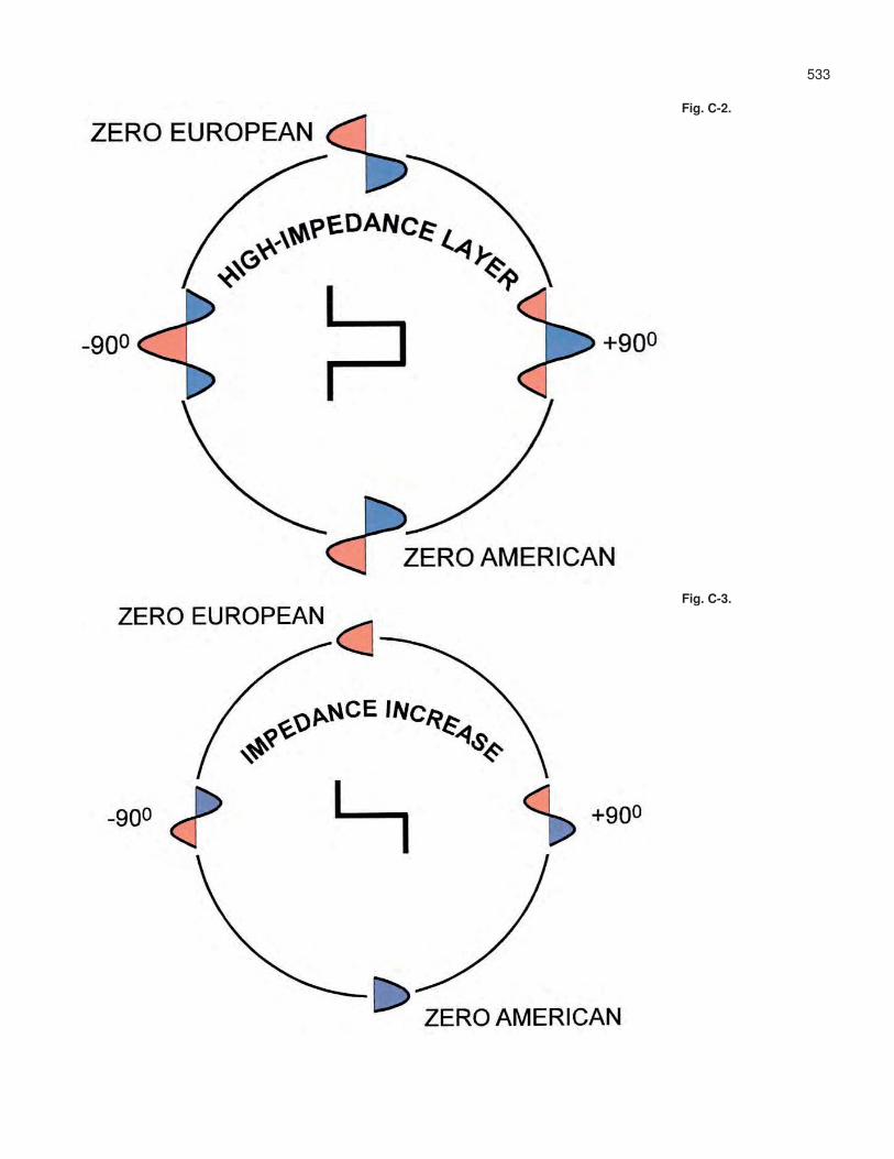
533

Fig. C-3.

Fig. C-2.

Summary ofRecommendations to HelpToday’s Interpreter GetMore Geology Out of 3-DSeismic Data in aReasonable Period of Time

• Expect detailed subsurface information

• Don’t rely on the workstation to find the solution

• Use all the data

• Understand the data and appreciate their defects

• Use time (or depth) slices/horizontal sections

• Visualize subsurface structure

• Use machine autotracking and snapping

• Select the color scheme with care

• Question data phase and polarity

• Tie seismic data to well data on character

• Try to believe seismic amplitude

• Understand the seismic attributes you use

• Prefer horizon attributes to windowed attributes

• Use techniques that maximize signal-to-noise ratio

534

APPENDIX D