Bank of Canada Working Paper 96-8 July 1996 Interpreting Money-Supply and Interest-Rate Shocks as Monetary-Policy Shocks by Marcel Kasumovich Department of Monetary and Financial Analysis Bank of Canada, Ottawa, Ontario, Canada K1A 0G9 [email protected](613) 782-8729 This paper is intended to make the results of Bank research available in preliminary form to other economists to encourage discussion and suggestions for revision. The views expressed are those of the author. No responsibility for them should be attributed to the Bank of Canada.
Transcript
Bank of Canada Working Paper 96-8
July 1996
Interpreting Money-Supply and Interest-Rate Shocks as
This paper is intended to make the results of Bank research available in preliminary form to othereconomists to encourage discussion and suggestions for revision. The views expressed are those ofthe author. No responsibility for them should be attributed to the Bank of Canada.
0-662-249408-9
Printed in Canada on recycled paper
ISSN 1192-5434
ISBN
Acknowledgments
The author would like to thank Robert Amano, Kevin Clinton, Pierre
Duguay, Charles Freedman, Scott Hendry, Jack Selody, and Pierre St-Amant
for comments and discussions. The contributions of Walter Engert and Ben
Fung were central to this paper. Naturally, the views expressed in this paper
are the author’s and should not be attributed to the Bank of Canada.
Abstract
In this paper two shocks are analysed using Canadian data: a money-supply shock(“M-shock”) and an interest-rate shock (“R-shock”). Money-supply shocks are derivedusing long-run restrictions based on long-run propositions of monetary theory. Thus, anM-shock is represented by an orthogonalized innovation in the trend shared by money andprices. An R-shock is represented by the orthogonalized innovation in the overnightinterest rate. Either type of shock might be interpreted as a monetary-policy shock.
A permanent increase in the nominal stock of M1 generates: a temporary fall in theinterest rate, consistent with the liquidity effect; a temporary rise in real output; apermanent increase in the price level; and a permanent depreciation of the nominalexchange rate. Although the behaviour of M1 is not directly controlled by the centralbank, the identifying assumption that the central bank controls the long-run trend inmoney and prices and has no long-run effect on real output appears to be quite reasonable.A temporary positive real-interest-rate shock generates a temporary fall in money andoutput, but prices rise initially (a “price puzzle”) before eventually declining. Both the M-shock and R-shock models are consistent with an active role for money in the transmissionof monetary policy.
Résumé
Dans le présent document, l’auteur analyse deux types de choc au moyen de donnéescanadiennes : un choc d’offre de monnaie (le choc M) et un choc de taux d’intérêt (le chocR). Pour identifier le premier type de choc, il recourt aux restrictions de long termedécoulant de certaines propositions avancées par la théorie monétaire. Le choc M estreprésenté par une innovation orthogonale dans la tendance commune qu’affichent lamonnaie et les prix, et le choc R, par une innovation orthogonale dans le taux d’intérêt àun jour. L’un ou l’autre de ces chocs peut être interprété comme un choc de politiquemonétaire.
Une augmentation permanente du stock nominal de monnaie, M1, entraîne lesconséquences suivantes: une chute temporaire du taux d’intérêt, conforme à l’effet deliquidité; une hausse passagère de la production exprimée en termes réels; uneaugmentation permanente du niveau des prix; et une dépréciation permanente du taux dechange nominal. Bien que le comportement de M1 ne soit pas contrôlé directement par labanque centrale, l’hypothèse que cette dernière détermine la tendance de la monnaie et desprix à long terme mais qu’elle n’exerce aucune influence sur la production en termes réelsen longue période semble fondée. Une hausse temporaire du taux d’intérêt réel provoqueune baisse temporaire de la masse monétaire et de la production, mais les prix affichent uncomportement plutôt déconcertant, puisqu’ils s’élèvent d’abord avant de redescendre. Lesrésultats obtenus à l’aide des modèles relatifs aux deux types de choc cadrent avec la thèsevoulant que la monnaie joue un rôle actif dans la transmission de la politique monétaire.
Central to the analysis of a monetary economy is the concept of the demand for money
(Friedman 1956). Temporal stability in the behaviour of the demand for money is of
particular interest for monetary policy. Given a stable demand-for-money function, a
stable path of monetary expansion will lead to a stable path for prices. However, the
empirical evidence of the stability of demand-for-money functions is mixed. Most
recently, Stock and Watson (1993) estimate M1 as a function of prices, real income and a
short-term interest rate using postwar U.S. data and find that the parameters of the
function are not stable over time. In contrast, restricting income elasticity to unity,
Hoffman, Rasche and Tieslau (1995) argue that the hypothesis of parameter stability
cannot be rejected for a similar function across five industrialized countries, including the
United States.
Even if the demand-for-money function is stable, there remains the issue of the
dynamic relationship between monetary policy actions and economic fluctuations.
Following the work of Lucas (1973) and Sargent and Wallace (1975), empirical research
on this issue has been attentive to unanticipated movements in monetary policy. The
application of vector autoregression (VAR) models and the identification of monetary-
policy shocks have recently dominated this research (for example, Sims 1980a, 1986;
Bernanke 1986; Keating 1992; Christiano and Eichenbaum 1992; Leeper and Gordon
1992; Lastrapes and Selgin 1995).
Monetary-policy shocks have been modelled as money-supply shocks, interest-rate
shocks and combinations of the two (for example, Cochrane 1994). Sims (1986) argues
that, since movements in M1 are the combination of private and central banking
behaviour, an M1 shock may not be an appropriate monetary-policy shock. Instead, Sims
argues that a Treasury-bill-rate shock is a more reasonable measure of a monetary-policy
shock. Similar to Sims (1986), Christiano and Eichenbaum (1992) use contemporaneous
restrictions to identify monetary-policy shocks. Using monetary base and M1 as the
measures of the money supply for quarterly and monthly U.S. data, they argue that money-
supply shocks lead to implausible interest rate and output movements. However, the
2
orthogonalized innovation in non-borrowed reserves, the central bank’s instrument of
monetary policy, could be interpreted as a monetary-policy shock.
Fung and Gupta (1994) identify a Canadian monetary-policy shock focussing on
the instruments of monetary policy. Of the two instruments of monetary policy —
settlement-balance management and open-market operations — settlement-balance
management is the primary instrument of monetary policy in Canada.1 Accordingly, Fung
and Gupta represent the orthogonalized innovation in excess settlement balances (excess
cash) as a monetary-policy shock. However, excess cash is difficult to motivate
empirically as a source of macroeconomic fluctuations, since it has properties very
different from typical monetary aggregates and has no discernible correlation with other
macro-variables. In addition, Fung and Gupta found that an unanticipated increase in
excess cash — an easing of monetary policy — was followed by a short-run fall in prices
(a “price puzzle”).2
Lastrapes and Selgin (1995) use long-run (Blanchard-Quah) restrictions to identify
money-supply shocks. They measure the money supply in the United States as monetary
base, M1 and M2. The authors find that a permanent money-supply shock generates a
temporary fall in interest rates, consistent with a monetary-policy shock. In contrast to the
conclusions when using contemporaneous restrictions, this result is common across the
different measures of the money supply. Thus, the dynamic effects of a U.S. monetary-
policy shock are sensitive to the identification strategy.
In this paper, we use the information from the central proposition of monetary
theory, the long-run demand-for-money function, as well as other restrictions to identify
two monetary-policy shocks: a money-supply shock and an interest-rate shock.3 Then,
1. In Canada the central bank controls the supply of deposits at the central bank held by financial institutions(settlement balances). Excess cash reserves are chartered bank deposits at the Bank of Canada in excess ofthe statutory minimum. (Reserve requirements were phased out between June 1992 and July 1994.)
2. However, in subsequent unpublished work, this price puzzle was not found when the overnight interestrate was used as the measure of monetary policy and the U.S. interest-rate instrument (the federal funds rate)was included in the central bank’s reaction function. (On this point, see Armour, Engert and Fung 1996.)
3. Fisher, Fackler and Orden (1995) identify a “monetary” shock using long-run cointegration restrictions.However, the authors do not examine the dynamics of interest rates or the exchange rate, which are central tothe conduct of monetary policy in a small open economy.
3
interpreting the supply of money in excess of its long-run demand as an indicator of the
stance of monetary policy, the dynamics of the transmission mechanism in the Canadian
economy are analysed. The long-run identification strategy is preferred since monetary
theory is built on long-run propositions. In this sense, relying on long-run restrictions is
considered to be less ad hoc than its contemporaneous counterpart.
The intuition of the money-supply shock is straightforward. Given a stable long-
run demand-for-money function, an orthogonalized innovation in the trend shared by
money and prices is interpreted as a money-supply shock (M-shock). That is, a monetary-
policy shock is interpreted as an exogenous disturbance to the common trend between
money and prices. This interpretation follows from the common-trends model developed
by King, Plosser, Stock and Watson (1987, 1991). In that model, a permanent productivity
shock is identified as the common stochastic trend in output, consumption, and
investment.
An M-shock under our representation does not mean that the central bank
exogenously creates or destroys M1, for example. Instead, it represents a central bank
action that disturbs the evolution of the trend shared by money and prices and that is not
accounted for by any other influences. This central bank action leads to a permanent
change in the nominal money supply and generates a new nominal equilibrium path in the
economy, with no long-run real economic consequences.
Armour, Engert and Fung (1996) argue that the orthogonalized innovation in the
overnight interest rate provides a good operational measure of monetary-policy shocks in
Canada. Thus, in addition to money-supply shocks, we also represent a monetary-policy
shock by the orthogonalized innovation in the overnight interest rate (R-shock).
To preview the results, we find that the M-shock models conform to a monetary-
policy shock. A permanent increase in the nominal stock of M1 generates: a temporary fall
in the interest rate, consistent with the liquidity effect; a temporary rise in real output; a
permanent increase in the price level; and a permanent depreciation of the nominal
exchange rate. The response of output is, however, negative for one quarter. The simple
M-shock models do not display short-run price and exchange-rate puzzles; a positive
4
money-supply shock leads to an increase in prices and a depreciation of the nominal
exchange rate. Thus although the behaviour of M1 is not directly controlled by the central
bank, the identifying assumption that the central bank controls the long-run trend in
money and prices and has no long-run effect on real output appears to be quite reasonable.
The R-shock models yield results that are broadly consistent with previous
literature: a temporary real-interest-rate shock generates a temporary fall in money and
output, but prices rise initially (a “price puzzle”) before eventually declining. Both the M-
shock and R-shock models are consistent with an active role for money in the transmission
of monetary policy.
Overall, the experiments, which focus on monetary-policy shocks defined in two
different ways and in a variety of model specifications, suggest the following four
principal conclusions:
• A long-run demand-for-M1 function is a robust feature of the data.
• A monetary-policy shock disturbs the relationship between money and itslong-run demand so as to create a long-lasting monetary disequilibrium.Consistent with Hendry (1995), such money gaps are eliminated over time asprices gradually adjust.
• Monetary-policy shocks clearly affect prices with a long lag (and the lag isvariable across the models considered here).
• A monetary-policy shock has a transitory effect on output but the effect may belong-lasting.
This paper is organized as follows. Section 2 reviews the role for money in the
transmission of monetary policy, as well as two long-run propositions of economic theory.
The empirical methodology, an adaptation of King, Plosser, Stock and Watson (1991), is
summarized in Section 4. Briefly, consistent with the propositions of economic theory,
cointegration relationships condition the matrix of long-run multipliers and define the
long-run restrictions in the VAR. The data and its properties are considered in Section 5.
The empirical results of the M-shock models and R-shock models are presented in
Sections 6 and 7. Finally, Section 8 summarizes the principal conclusions of the paper.
5
2. Money in the Transmission Mechanism
2.1 Alternative views of money
According to one view of the monetary transmission mechanism, the monetary authority
controls a short-term interest rate and the nominal quantity of money evolves
endogenously and passively according to its demand. In this case, money is a passive
channel with no meaningful causal role in the transmission of monetary policy.
In an alternative approach, discrepancies between the nominal quantity of money
demanded and the nominal quantity of money supplied are pivotal to the analysis of the
transmission mechanism (Friedman 1970). According to an active-money view, while the
quantity of money may be endogenous, it is also subject to the independent influence of
the central bank. This influence, among other things, can lead to a real quantity of money
holdings that is larger (smaller) than desired. In contrast to the passive-money view, the
attempt to eliminate these excess balances (restore deficient balances) is considered to
have an important role in the transmission of monetary policy.
The interpretation of a nominal “monetary shock” highlights the distinction
between the two views. According to the passive-money view, a monetary shock is the
consequence of a change in the demand for money (caused by an output shock, for
example) that is accommodated by the central bank as it targets short-term interest rates.
In contrast, the active-money view interprets a monetary shock as the consequence
of a change in the supply of money induced by the central bank that is unanticipated by
agents. Consider a positive shock: initially, agents have to hold the additional nominal
balances.4 Over time, individuals perceive that the nominal quantity of money they hold
4. As an example of an active-money view, proponents of the “buffer-stock view” argue that money bal-ances are used by agents to absorb unanticipated variations in income flows. For example, expansionarymonetary shocks, generating a short-run fall in interest rates, can lead to changes in the expected returns of aplanned portfolio. In the time that it takes to choose an alternative portfolio, average money holdingsincrease. (A similar example can be constructed for consumption decisions.) While this increase may seemtrivial for the individual, it is argued that, in the aggregate, the increase in money holdings is important. Fora further examination of the buffer-stock view, see Johnson (1962), Carr and Darby (1981) and Laidler(1990, 1994).
6
corresponds to a real quantity that is larger than desired, at current prices, and that this is
not a temporary condition. That is, individuals are “off” their long-run demand-for-money
function. However, all individuals cannot collectively dispose of theaggregate excess
nominal balances. Nonetheless, the attempt to do so has economic effects. The increase in
expenditure leads to an increase in nominal spending, an increase in economic activity,
and ultimately an increase in prices. This transmission continues until the factors affecting
the supply and the demand for money adjust to restore monetary equilibrium.
These alternative views of money in the transmission mechanism — the passive-
money and the active-money views — can be distinguished by dynamic empirical
analysis. There are, for example, two distinguishing features of these two views. First, the
active-money view suggests that there is a tendency for discrepancies between the nominal
quantity of money demanded and the nominal quantity of money supplied to persist.
According to the passive-money view, instantaneous interest-rate adjustments eliminate
any excess money balances. A second distinguishing feature is that the active-money view
argues that individuals’ attempts to eliminate such monetary disequilibriums have
aggregate short-run economic consequences. The passive-money view makes no similar
claims.
Given the brief discussion of the role of money in the transmission mechanism, the
following subsection reviews some simple long-run propositions of economic theory.
2.2 Long-run propositions of economic theory
Demand for money
Views about money in the transmission mechanism presume the existence of a long-run
demand-for-money function. In the aggregate, the demand for real money balances is
thought to increase with real economic activity. The opportunity cost of holding real
balances — the foregone investment income (real rate of interest) and the lost purchasing
power over the holding period (expected rate of inflation) — is summarized by the
nominal rate of interest. Thus, the long-run demand for money can be expressed as
7
(2.1)
where is the log of the nominal stock of money, is the log of the price level, is the
log of real output and is the nominal rate of interest.
The demand-for-money function has an empirical interpretation. It is well
documented that the variables described in (2.1) are non-stationary. If, however, relation
(2.1) is stationary, then the long-run demand for money can be interpreted as a
cointegration relationship.
Open-economy propositions
For the dynamic analysis of a small open-economy like Canada, consideration of open-
economy equilibrium propositions is necessary. Since the demand for money is thought of
as (virtually) independent of the openness of the economy, a respecification of this
function is, in general, unnecessary.5 Moreover, with flexible exchange rates, domestic
nominal variables are determined by domestic policy, assuming aggregate supply and real
interest rates are determined on the real side of the economy, including international
developments. Consequently, the role of the exchange rate is the primary focus of the
open-economy propositions.
Open-economy propositions rely on the competitiveness of domestic goods and
the mobility of domestic capital in world markets. By the “law of one price,” competition
in goods markets and capital mobility in capital markets imply that, at least in the long
run, no arbitrage opportunities can exist by trading domestic goods (capital) for identical
foreign goods (capital).
Purchasing power parity (PPP) summarizes the law of one price for goods markets:
the domestic price and foreign price of the same good will be equal, adjusted for the
5. McKinnon (1982), Poloz (1984, 1986) and Filosa (1995) admit the possibility of money holders shiftingamong currencies. In these “currency substitution” models, the expected depreciation of domestic currencyis included in the demand-for-money function.
md
p– β1y β2– R=
m p y
R
8
exchange rate between the two currencies. Thus, one role of the exchange rate is to
reconcile movements of foreign and domestic prices. PPP can be expressed as
(2.2)
where is the log of the foreign price level and is the log of the price of domestic
currency relative to foreign currency. The PPP relationship has an empirical interpretation
similar to that of the demand-for-money function. Although the relationship may not hold
at any given point in time, if (2.2) is stationary, then in the long run PPP describes the
equilibrium real exchange rate.
Interest-rate parity (IRP) summarizes the law of one price for capital markets: the
domestic nominal rate of interest will be equal to the foreign nominal rate of interest,
adjusted for the expected rate of change in the exchange rate between the two currencies,
abstracting from risk premiums. IRP can be expressed as
(2.3)
where is the foreign nominal rate of interest and is the expected rate of
change in the exchange rate. (The empirical interpretation of IRP is parallel to the demand
for money and PPP cases.)
In order to interpret shocks with causal inference (an economic interpretation),
dynamic empirical analysis requires a set of identification assumptions. The above
propositions, central to the monetary analysis of an open economy, are straightforward,
although questionable. The question of how to use this long-run information in a set of
identification restrictions is a methodological issue addressed in the following section.
PFX p pf
–=
pf
PFX
E ∆PFX( ) R Rf
–=
Rf
E ∆PFX( )
9
3. Empirical Methodology
The purpose of this section is to briefly discuss alternative identification strategies and
then show how the long-run propositions of monetary theory are used to identify
economic shocks through long-run restrictions.6
3.1 Alternative identification strategies
Define as the vector of economic variables and as the vector of serially
uncorrelated disturbances with covariance matrix . A linear characterization of the
economy can be described by the following structural autoregressive model:
(3.1)
where is an unknown matrix of parameters and the number of autoregressive
lags is truncated to . It is assumed that the researcher knows the following reduced-form
model
(3.2)
where and . Since model (3.2) is estimated, we know the ’s
and . The distinguishing feature of models (3.1) and (3.2) is the matrix of
contemporaneous relationships . In terms of the classical identification problem,
additional assumptions are required to recover model (3.1) from model (3.2).
Common to the literature on VAR models, a recursive causal chain can be assumed
(Sims 1980b). Ordering the variables in terms of their causal importance implies that the
matrix of contemporaneous relationships is lower triangular (a Wold ordering). In a two-
variable system of prices and money, for instance, a prices-money ordering assumes that,
6. This section provides an intuitive discussion of the identification strategy used in this paper. Readersinterested only in the results can skip to Section 4. The algebraic detail of the empirical methodology is pro-vided in Appendix 2.
Xt n 1× εt n 1×
Σε
D0Xt D1Xt 1– … Dl Xt l– εt+ + +=
Di n n×
l
Xt H1Xt 1– … Hl Xt l– et+ + +=
Hi D01–Di= et D0
1– εt= Hi
et
D0
10
contemporaneously, money responds to price shocks but prices do not respond to money
shocks.
A fundamental criticism of the Wold ordering is the inability to interpret the
shocks (Cooley and Leroy 1985). Relying on well-defined economic theory as the
constraining structure in a VAR model addresses the Cooley-Leroy criticism. In this
regard, several empirical studies impose structure implied by the contemporaneous
predictions of economic theory. In a four-variable model of money, prices, output and
interest rates, the identification strategy used by Keating (1992), for example, includes a
short-run demand-for-money function. The long-run predictions of economic theory have
also been used in identification strategies. For example, in a bivariate model of output and
unemployment, Blanchard and Quah (1989) assumed that fluctuations in GDP are
characterized by two types of shocks: those that have a (long-run) permanent effect on
output and those that do not.
A long-run identification strategy can be an appropriate device for analysing the
dynamics of the monetary transmission mechanism for two primary reasons. First, as a
theoretical matter, competing views of the role of money in the transmission mechanism
rely on long-run propositions. In the short run, however, economic theory does not
necessarily predict these propositions will hold. In this sense, relying on long-run structure
is considered to be less ad hoc than its contemporaneous counterpart.7 Second, as an
empirical matter, it is well-documented that several macro-variables can be characterized
as unit-root processes; that is, the variables are subject to a stochastic trend (for example,
Nelson and Plosser 1982). This implies that shocks to these variables havepermanent
effects. Many of these same variables share stochastic trends, implying the existence of a
stationary linear combination of the variables; that is, the variables are cointegrated (Engle
and Granger 1987). This mean-reversion (or trend-reversion) property implies that shocks
to the combination of the variables have onlytemporary effects. We argue, therefore, that
a long-run identification strategy can best exploit the theoretical and empirical properties
of the macro-variables.
7. Long-run restrictions do, however, make the strong assumption that, contemporaneously, the central bankobserves all the variables included in the VAR model (see Faust and Leeper 1994).
11
As a result of these considerations, this paper uses the cointegration structure,
which is consistent with monetary theory, as the primary vehicle of identification.
3.2 Estimation of the VAR and the long-run cointegration restrictions
By simple algebra, model (3.2) can be rewritten in error-correction form as
(3.3)
where is the first difference operator, and . This
representation is convenient for a system of equations where the components of are
difference-stationary and cointegrated. In that case, can be decomposed into two full
column rank matrices such that , where and are matrices and
. The stationary combinations of the non-stationary variables are represented by
and describe the low-frequency relationships in the system (long-run equilibrium).
That is, the columns of represent the cointegration vectors. The elements of the
matrix are the adjustment parameters. Any deviation from long-run equilibrium results
in a change in that is consistent with the system returning to equilibrium. The path to
equilibrium is described by the short-run dynamics of the model, the parameters of the
lagged endogenous variables. Following Johansen and Juselius (1990), tests of the
cointegration rank (rank of ) are performed and the parameters of the cointegration
vectors are estimated. Then, the remaining parameters of model (3.3) are estimated by
ordinary least squares (OLS).
After estimating model (3.3), we can generate the following reduced-form
moving-average representation (MAR):
(3.4)
∆Xt Γ1∆Xt 1– … Γl 1– ∆Xt l– 1+ πXt l– et+ + + +=
∆ Γi I– n H jj 1=
i
∑+= Γl π=
X
π
π αβ'= α β n r×
0 r n< <
β'Xt l–
r β
α
X
β
∆Xt G L( )et=
12
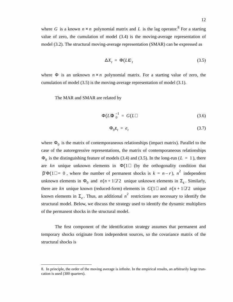
where is a known polynomial matrix and is the lag operator.8 For a starting
value of zero, the cumulation of model (3.4) is the moving-average representation of
model (3.2). The structural moving-average representation (SMAR) can be expressed as
(3.5)
where is an unknown polynomial matrix. For a starting value of zero, the
cumulation of model (3.5) is the moving-average representation of model (3.1).
The MAR and SMAR are related by
(3.6)
(3.7)
where is the matrix of contemporaneous relationships (impact matrix). Parallel to the
case of the autoregressive representations, the matrix of contemporaneous relationships
is the distinguishing feature of models (3.4) and (3.5). In the long-run ( ), there
are unique unknown elements in (by the orthogonality condition that
, where the number of permanent shocks is ), independent
unknown elements in and unique unknown elements in . Similarly,
there are unique known (reduced-form) elements in and unique
known elements in . Thus, an additional restrictions are necessary to identify the
structural model. Below, we discuss the strategy used to identify the dynamic multipliers
of the permanent shocks in the structural model.
The first component of the identification strategy assumes that permanent and
temporary shocks originate from independent sources, so the covariance matrix of the
structural shocks is
8. In principle, the order of the moving average is infinite. In the empirical results, an arbitrarily large trun-cation is used (300 quarters).
G n n× L
∆Xt Φ L( )εt=
Φ n n×
Φ L( )Φ01–
G L( )=
Φ0εt et=
Φ0
Φ0 L 1=
kn Φ 1( )
β'Φ 1( ) 0= k n r–= n2
Φ0 n n 1+( ) 2⁄ Σε
kn G 1( ) n n 1+( ) 2⁄
Σe n2
13
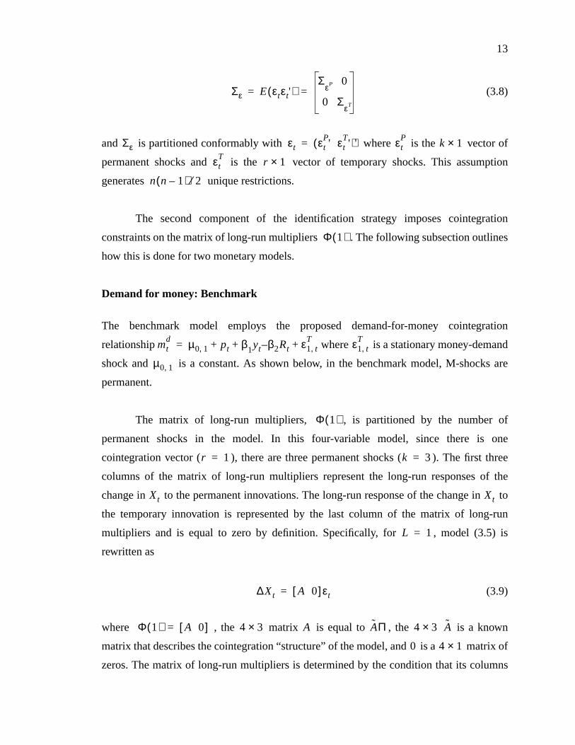
(3.8)
and is partitioned conformably with where is the vector of
permanent shocks and is the vector of temporary shocks. This assumption
generates unique restrictions.
The second component of the identification strategy imposes cointegration
constraints on the matrix of long-run multipliers . The following subsection outlines
how this is done for two monetary models.
Demand for money: Benchmark
The benchmark model employs the proposed demand-for-money cointegration
relationship where is a stationary money-demand
shock and is a constant. As shown below, in the benchmark model, M-shocks are
permanent.
The matrix of long-run multipliers, , is partitioned by the number of
permanent shocks in the model. In this four-variable model, since there is one
cointegration vector ( ), there are three permanent shocks ( ). The first three
columns of the matrix of long-run multipliers represent the long-run responses of the
change in to the permanent innovations. The long-run response of the change in to
the temporary innovation is represented by the last column of the matrix of long-run
multipliers and is equal to zero by definition. Specifically, for , model (3.5) is
rewritten as
(3.9)
where , the matrix is equal to , the is a known
matrix that describes the cointegration “structure” of the model, and is a matrix of
zeros. The matrix of long-run multipliers is determined by the condition that its columns
Σε E εtεt'( )Σ
εP 0
0 ΣεT
= =
Σε εt εtP' εt
T'( )'= εt
Pk 1×
εtT
r 1×
n n 1–( ) 2⁄
Φ 1( )
mtd µ0 1, pt β+ 1yt β2– Rt ε1 t,
T+ += ε1 t,
T
µ0 1,
Φ 1( )
r 1= k 3=
Xt Xt
L 1=
∆Xt A 0[ ]εt=
Φ 1( ) A 0[ ]= 4 3× A AΠ 4 3× A
0 4 1×
14
are orthogonal to the cointegration relations so that (Engle and Granger
1987). The partition of the matrix of long-run multipliers, combined with the
orthogonality condition, generates (unique) identification restrictions. The matrix is
a lower triangular matrix with full column rank and diagonal elements normalized to
one. contains unknown elements and identification
restrictions (a long-run recursive Wold ordering). This matrix is the normalization used to
distinguish permanent shocks; the restrictions associated with exactly identify the
permanent components of the model.9 From the assumption that the permanent shocks are
mutually uncorrelated, the unknown parameters of can be determined (see
Appendix 2).10
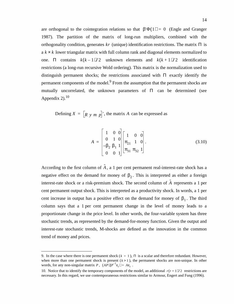
Defining , the matrix can be expressed as
. (3.10)
According to the first column of , a 1 per cent permanent real-interest-rate shock has a
negative effect on the demand for money of . This is interpreted as either a foreign
interest-rate shock or a risk-premium shock. The second column of represents a 1 per
cent permanent output shock. This is interpreted as a productivity shock. In words, a 1 per
cent increase in output has a positive effect on the demand for money of . The third
column says that a 1 per cent permanent change in the level of money leads to a
proportionate change in the price level. In other words, the four-variable system has three
stochastic trends, as represented by the demand-for-money function. Given the output and
interest-rate stochastic trends, M-shocks are defined as the innovation in the common
trend of money and prices.
9. In the case where there is one permanent shock ( ), is a scalar and therefore redundant. However,when more than one permanent shock is present ( ), the permanent shocks are non-unique. In otherwords, for any non-singular matrix , .
10. Notice that to identify the temporary components of the model, an additional restrictions arenecessary. In this regard, we use contemporaneous restrictions similar to Armour, Engert and Fung (1996).
β'Φ 1( ) 0=
kr Π
k k×
Π k k 1–( ) 2⁄ k k 1+( ) 2⁄
Π
k 1= Πk 1>
P AP( ) P1– εt( ) Aεt=
Π
r r 1+( ) 2⁄
X R y m p'= A
A
1 0 0
0 1 0
β– 2 β1 1
0 0 1
1 0 0
π21 1 0
π31 π32 1
=
A
β2
A
β1
15
Combined with , the matrix of long-run multipliers implies that a real-interest-
rate shock can have a permanent effect on all other variables, that productivity shocks have
no long-run interest-rate effects but can effect (real) money and prices in the long-run, and
that money shocks have a long-run impact on prices only.
Demand for money: Open-economy extension
The open-economy extension of the benchmark model includes the purchasing-power-
parity relationship where is a stationary real exchange-
rate shock and is a constant. Defining , where is
restricted to be strictly exogenous, the matrix of long-run multipliers for the five
endogenous variables can be summarized as
. (3.11)
The first column of represents a 1 per cent foreign price-level shock; this leads to a
1 per cent appreciation of domestic currency (a decrease in the exchange rate). The next
two columns of the matrix correspond to the interest-rate and productivity shocks in the
benchmark model. The fourth column describes a domestic money shock but differs from
the benchmark model in that it leads to a depreciation of domestic currency (an increase in
the exchange rate). As in the benchmark model, money-supply shocks have no long-run
real economic consequences.
Π
PFXt µ0 2, p+ t ptf
– ε2 t,T
+= ε2 t,T
µ0 2, X pf
PFX R y m p'= pf
A
1– 0 0 1
0 1 0 0
0 0 1 0
0 β– 2 β1 1
0 0 0 1
1 0 0 0
π21 1 0 0
π31 π32 1 0
π41 π41 π43 1
=
A
A
16
4. The Data
In general, for classical statistical inference, stationarity is a necessary property.
Therefore, after determining the variables’ order of integration, the highest order of
integration in the variable set is transformed to one (that is, I(1)). The cointegrating
combinations of the non-stationary variables will then necessarily be I(0). In terms of an
error-correction model, since all of the components are stationary, we are able to test the
proposed theoretical cointegration relations using standard distribution theory.
The data used in this study are quarterly observations. The domestic data set is an
overnight rate of interest ( ); gross domestic product (in logarithms, ); the consumer
price index (in logarithms, ); net nominal M1 balances, defined as currency plus
chartered bank net demand deposits (in logarithms, ); and the Canadian dollar price of
the U.S. dollar (in logarithms, ). The foreign data set is the federal funds rate ( )
and the U.S. gross domestic product deflator (in logarithms, ).11 The sample period for
the regressions is 1954Q3 to 1994Q4 for systems defined in terms of the price level, and
1954Q4 to 1994Q4 for systems specified in terms of inflation.
Univariate analysis indicated that the data set was I(1), with two exceptions: in the
case of prices, there was evidence supporting either an I(1) or an I(2) process; and the
ex post real interest rate could be either I(1) or I(0). In examining a role for money, in
particular a demand-for-money relationship, Stock and Watson (1993) found similar
results for U.S. data (both the net national product price deflator and U.S. nominal money
supply (M1) were either I(1) or I(2)). Given the indeterminate results, two systems are
analysed depending on the order of integration of the price level (and the money supply).
The first set of models is based on prices being I(1); the second set of models is
based on prices being I(2), so that the inflation rate (which is I(1)) is the relevant variable
for the VAR.
11. From 1954Q3 to 1971Q1 is the average of the day-to-day loan rate. From 1971Q2 to 1995Q1 is theaverage overnight financing rate. GDP is expenditure-based, in millions of 1986 Canadian dollars. The nom-inal money supply is the average of the last Wednesday of the month, in millions of dollars. The nominalexchange rate is the average of the end-of-month closing price. The U.S. interest rate is the average of theend-of-month observations.
R y
p
m
PFX Rf
pf
R R
17
5. M-shock Models: Estimation Results
In this section, we estimate the error-correction model and generate impulse response
functions. This is done in three steps. First, we test for the number of cointegration vectors
and estimate their parameters (using the Johansen and Juselius (1990) methodology
combined with the finite sample critical values generated in Appendix 3). Second, the
proposed theoretical cointegration relationships are tested. In the third step, the parameter
estimates of the cointegration vectors (as well as other restrictions) are used to identify the
economic shocks and the impulse response functions are then examined.
5.1 Demand for money: Benchmark
The benchmark model employs the demand-for-money cointegration relationship
and defines whereD81 is a
linear deterministic shift parameter.12 For the purposes of cointegration analysis, we first
assume that the price level is integrated of order one (which implies that the ex post real
interest rate is also integrated of order one, since the nominal interest rate is I(1)). The
following subsection summarizes the tests for the number of permanent innovations in the
system and estimates the parameters of the demand-for-money function.
Cointegration results
The cointegration results are summarized in Table 1 (Appendix 1). Following Johansen
and Juselius (1990), the maximum eigenvalue and trace tests are used to determine the
number of stochastic trends in model (3.3) (the number of permanent innovations).13
Based on finite-sample critical values, the system is concluded to have at least two
12. Hendry (1995) illustrated that the relationship between money, prices, output and interest rates is stablewith the inclusion of a linear deterministic shift parameter that accounts for the financial innovation from1980 to 1983.
13. An adaptation of the likelihood-ratio test was used to determine the optimal lag structure of the models.DeSerres and Guay (1995) show that, for the purposes of imposing long-run restrictions, this sequential testis preferred to information criteria (such as the Akaike criteria). The optimal lag structure (l) for the bench-mark model is six. The optimall for the open-economy extension is four.
mtd µ0 1, pt β+ 1yt β2– Rt γD81 ε1 t,
T+ + += X R y m p'=
18
stochastic trends (at most two cointegration vectors).14 In the benchmark model, the
demand-for-money function is considered as the unique cointegration vector. Thus, we
restrict the cointegration space to one vector. This vector can easily be interpreted as a
demand-for-money function. The hypothesis of unitary-price elasticity cannot be rejected
(p-value 0.22), the income elasticity of 0.70 is (significantly) less than one and the
interest-rate semi-elasticity is -0.04. According to the statistically significant adjustment
parameters, changes in money and prices eliminate a deviation of money from its desired
level.
Given the parameter estimates of the demand-for-money function, the restrictions
to the matrix of long-run multipliers allow for the dynamic analysis of the permanent
innovations in the system. With respect to a monetary-policy shock, the following
experiment is considered: an unanticipated contemporaneous movement in monetary
policy that generates a 1 per cent permanent change in the nominal equilibrium path of the
economy. The following subsection summarizes the impulse response functions.
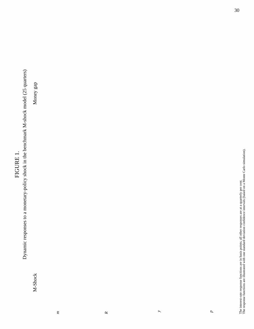
Impulse responses to the M-shock
In response to a positive M-shock, money increases gradually to the new nominal
equilibrium (Figure 1, column 1). The intuition of the response function is clear. Since the
endogenous properties of the money stock are known by the central bank (estimated by
model (3.3)), in order to induce a 1 per cent permanent change in the money stock, the
central bank need only induce a contemporaneous change of 0.36 per cent. This can be
interpreted as a multiplier effect.
Consistent with a liquidity effect, the overnight interest rate responds to the M-
shock with a significant decrease for three quarters.15 Output responds positively and
significantly after four quarters. At the sixth quarter, the output response peaks (0.2 per
14. Appendix 3 summarizes the methodology for generating asymptotic and finite-sample critical valuesbased on a system with the intercept term and the deterministic variableD81 restricted to the cointegrationspace. The finite-sample values lead to (at times) vastly different conclusions with respect to the dimension-ality of the cointegration space.
15. For the analysis of the impulse response functions, “significant” will mean “statistically significantlydifferent from zero.” This corresponds to the case where the one-standard-deviation confidence bands of theresponse function lie on one side of the x-axis (which represents a zero response).
19
cent) and then decreases back to steady state. The impact response of the price level is
quite sluggish (0.06 per cent); the response of the price level increases gradually towards
steady state. Figure 1 (column 2) plots the deviation of money from its long-run demand.
This “money gap” is long-lasting. Following an M-shock, monetary disequilibrium is
above 0.4 per cent for seven quarters. One interpretation of the positive deviation of
money from its long-run demand is that the supply of money is moving independently of,
rather than in response to, the demand for money. The restoration of monetary equilibrium
appears most closely related to the equilibrium adjustment of the price level.
The majority of previous empirical work has represented a money-supply shock as
the orthogonalized component of the innovation in a monetary aggregate (for example,
Christiano and Eichenbaum 1992). In contrast, in this paper, an unanticipated
contemporaneous increase in the money supply leads to a permanent change in the
nominal equilibrium path of the economy; however, a money-demand shock, which is
transitory, leads to only a temporary deviation from equilibrium (by virtue of the
cointegration restrictions). This may explain why, in previous empirical work, temporary
money shocks behave like money-demand innovations.
Several VAR-based studies of monetary-policy shocks find a “price puzzle.” For
example, Sims (1992) finds that a positive interest-rate shock leads to an increase in prices
in several industrialized countries. He argues that this puzzle may be the endogenous
policy response to inflationary pressures that are observed by the central bank but that are
not included in the model. Fung and Gupta (1994) find a counterintuitive price response in
Canada. However, the simple M-shock model does not give rise to this puzzle. This
suggests that the price puzzle may be the result of the contemporaneous identification
strategy and the measure of monetary policy used in previous studies.
5.2 Demand for money: Open-economy extension
The open-economy model extends the benchmark model with the inclusion a purchasing-
power-parity cointegration relationship . In this model
and is strictly exogenous. Thus domestic shocks are
restricted to have no impact on the foreign price level. In addition, following a domestic
PFXt µ0 2, p+ t ptf
– ε2 t,T
+=
X pf
PFX R y m p'= pf
20
shock, purchasing power parity is restored through the reaction of the domestic price level
and the nominal exchange rate.
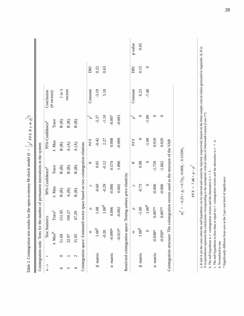
Cointegration results
The cointegration results are summarized in Table 2 (Appendix 1). The maximum
eigenvalue and trace tests support three to five stochastic trends in the system (one to three
cointegration vectors). The open-economy model is considered to have two cointegration
vectors. Thus, we restrict the cointegration space to two vectors. The first vector can easily
be interpreted as a demand-for-money function with an income elasticity of 0.73 and an
interest-rate semi-elasticity of . The joint restrictions associated with the money-
demand and purchasing-power-parity relationships, as well as the zero restriction on the
speed of adjustment parameters of foreign prices, are rejected by the data (p-value 0.05).
Maintaining the assumption of output-neutrality from the benchmark model, we assume
that monetary-policy shocks do not have a long-run effect on the real exchange rate. That
is, we assume that monetary-policy shocks are not the source of non-stationarity in the real
exchange rate.
The experiment conducted is the same as in the benchmark model: a monetary-
policy shock that generates a 1 per cent permanent change in the nominal equilibrium path
of the economy. The following subsection summarizes the impulse response functions in
comparison with the benchmark model.
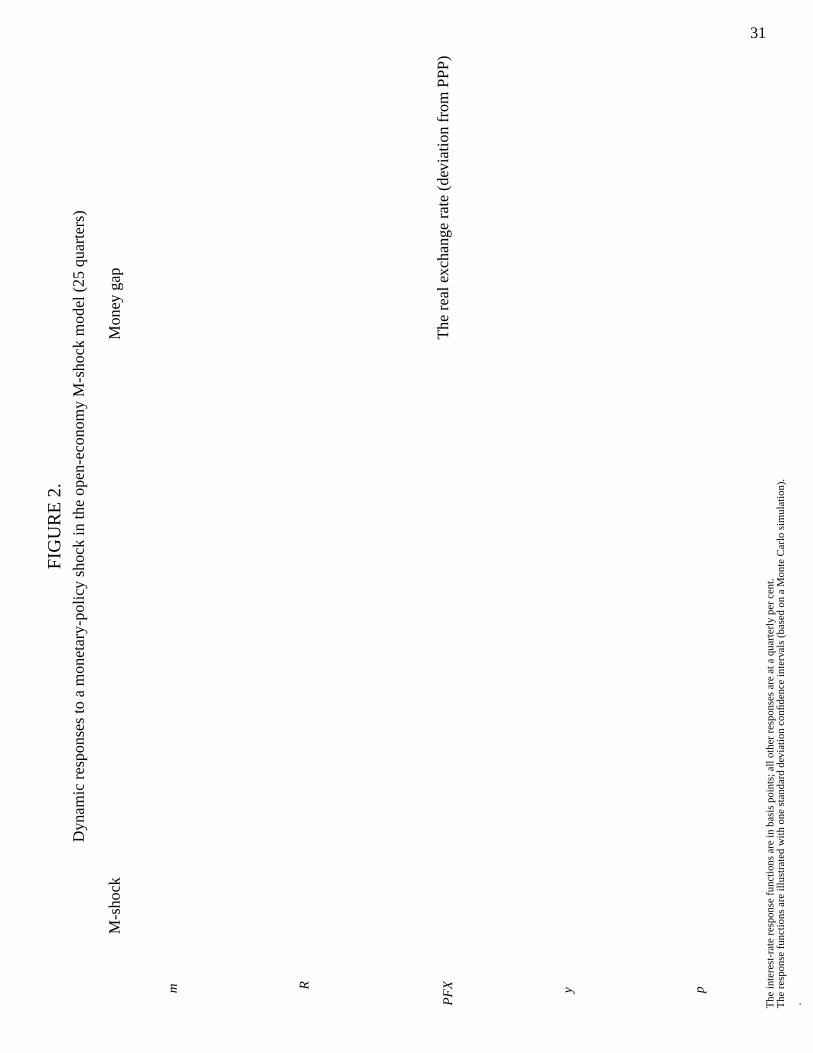
Impulse responses to the M-shock
In response to a positive M-shock, money adjusts to the new nominal equilibrium after
four quarters, much faster than in the benchmark model (Figure 2, column 1). This may
explain one role of the exchange rate in the transmission of monetary policy: exchange-
rate fluctuations allow the stock of money to reach equilibrium faster than would
otherwise be the case.
The overnight interest rate initially responds with a significant decrease (25 basis
points). This liquidity effect lasts for about four quarters and is very similar to that of the
benchmark model. Output responds positively after two quarters; the effect on output is
0.08–
21
transitory but long-lasting. The nominal exchange rate depreciates contemporaneously by
0.29 per cent and then continues to depreciate towards the new nominal equilibrium. As
expected, the money-supply shock affects the exchange rate more quickly than it does
prices in the goods market, as measured by the consumer price index; the
contemporaneous increase in the price level is significant but small (0.07 per cent). Figure
2 (column 2) plots the response of the two equilibrium conditions of the model: the
demand-for-money and the purchasing-power-parity relationships. As in the benchmark
model, the equilibrium adjustment of the price level appears most closely related to the
monetary disequilibrium. The real-exchange-rate deviation from parity is above 20 basis
points for over 9 quarters. This overshooting, which occurs because the equilibrium
adjustment of the nominal exchange rate is faster than the price level, may be the source of
the long-lasting output effect following the money-supply shock.
In addition to the short-run response of the price level, a second puzzle for VAR-
based studies of monetary-policy shocks is the “exchange-rate puzzle.” Grilli and Roubini
(1995), for example, find that a positive interest-rate shock leads to a depreciation of the
exchange rate for all G-7 countries other than the United States. However, the M-shock
model generates an intuitive nominal exchange-rate response. This suggests that the
exchange-rate puzzle also may be the result of the contemporaneous identification strategy
and the measure of monetary policy used in previous studies.
The M-shock models are consistent with the view that money plays an active role
in the transmission of monetary policy. The slow equilibrium adjustment of the models
suggests that monetary policy can have real short-run economic effects. The models also
help explain the role of the interest rate and the exchange rate in the monetary
transmission mechanism. The similarity between the interest-rate dynamics in the two M-
shock models suggests that the central bank manipulates a quantity instrument (such as
settlement balances) in order to attain a particular interest-rate path. Nominal exchange-
rate fluctuations allow the stock of money to adjust more quickly than would otherwise be
the case. However, since the equilibrium adjustment of the nominal exchange rate is faster
than the price level, the real exchange rate overshoots. Thus, a monetary-policy shock can
have long-lasting output effects.
22
6. An Alternative Specification of Monetary-Policy Shocks:R-Shock Model Estimation Results
An interest-rate shock (R-shock) can also be interpreted as a monetary-policy shock, as in
several VAR-based studies. The overnight interest rate makes a relatively attractive
monetary-policy variable because it is subject to considerable influence by the central
bank. (However, it is not a variable that is under the central bank’s control.) In the
identification strategy for the R-shock model, we maintain the assumption that a
monetary-policy shock has no long-run real economic consequences. Thus the appropriate
R-shock is considered to be atemporary real-interest-rate shock which has onlytemporary
economic effects. In the remainder of this section, we analyse such a shock in an open-
economy model.
6.1 Demand for money and R-shocks
In Section 5, the real interest rate was assumed to be integrated of order one. However, if
inflation is I(1), then cointegration between the nominal interest rate and the rate of
inflation would imply that the real interest rate is I(0). The evidence of the order of
integration of the real interest rate was mixed. Univariate unit-root tests could not reject a
non-stationary real rate. In a multivariate model of real money, output, interest rates and
inflation, however, there was evidence of cointegration between the nominal interest rate
and the rate of inflation.
We consider an R-shock in the context of an open economy. In particular, relying
on the parity conditions PPP and IRP, an R-shock is represented as a monetary-policy
action that generates a temporary deviation from the equilibrium real interest rate, where
the equilibrium real interest rate is the cointegration relationship between domestic and
foreign real interest rates. This interpretation of an R-shock can accommodate either an
I(0) or I(1) domestic/foreign real interest rate. For the I(0) case, cointegration between
domestic and foreign real interest rates is redundant; a temporary R-shock is adequately
represented as an innovation in the domestic real interest rate. For the I(1) case, a real-
interest-rate shock is non-stationary and may therefore have permanent economic effects.
However, cointegration between the domestic and foreign real interest rates implies that
23
domestic R-shocks are stationary, representing a temporary deviation from the non-
stationary foreign real interest rate.
In this model, there are two cointegration relationships to consider. First, the
demand-for-money function is expressed as
(7.1)
where is a stationary money-demand shock (temporary shock). The second
relationship follows from PPP and IRP. Applying the first-difference operator to the PPP
relationship (equation (2.2)) and combining it with the IRP relationship (equation (2.3)),
the (long-run) equilibrium real interest rate can be expressed as
(7.2)
where is a stationary real-interest-rate shock (temporary shock). An R-shock is a
monetary-policy action that generates a temporary deviation from the equilibrium real
interest rate.
As in the M-shock models, the structure of the R-shock model is summarized by
the two cointegration relationships, (7.1) and (7.2). In this model,
and the foreign variables, and , are restricted to
be strictly exogenous. Thus, domestic shocks are restricted to have no impact on the
foreign inflation rate and the foreign nominal rate of interest. In addition, following a
domestic shock, the equilibrium real rate of interest is restored through the reaction of the
domestic inflation rate and the domestic nominal interest rate.
The matrix of long-run multipliers is partitioned by the number of permanent
shocks in the model; in this six-variable system, there are two hypothesized temporary
shocks and four hypothesized permanent shocks. As in the M-shock model, the
cointegration relationships impose restrictions on the matrix of long-run multipliers.
These restrictions are used to interpret the permanent shocks in the model. In this system,
mtd
pt– µ0 1, β1yt β2– Rt γD81 ε1 t,T
+ + +=
ε1 t,T
Rt Et pt 1+∆–( ) µ0 2, Rtf
Et∆ pt 1+f
–( ) ε2 t,T
+ +=
ε2 t,T
X Rf ∆ p
fy ∆p R m p–( ) '= R
f ∆ pf
24
the four hypothesized permanent shocks are: an output shock, a neutral domestic inflation
shock, a neutral foreign inflation shock and a foreign real-interest-rate shock. There are
two hypothesized temporary shocks: a money-demand shock and a real-interest-rate
shock.
However, as discussed in Section 3, the long-run restrictions are not sufficient to
identify the temporary shocks in the model. Thus, additional restrictions are required. In
this regard, an interest-rate shock is assumed to have a contemporaneous impact on only
real money balances.
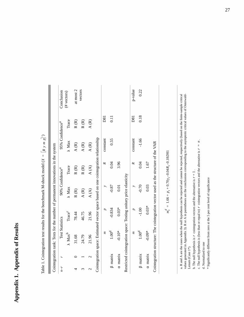
Cointegration results
The cointegration results are summarized in Table 3 (Appendix 1). The system has three
to five permanent innovations (one to three cointegration vectors). The restrictions
corresponding to equations (7.1) and (7.2) could not be rejected (not shown, p-value 0.40).
However, the joint test of the restrictions associated with equations (7.1) and (7.2) and the
zero restrictions on the speed of adjustment parameters of the foreign variables were
rejected by the data (p-value 0.004). Nonetheless, we restrict the foreign variables to be
(strictly) exogenous when generating the impulse response functions.
The estimates of the demand-for-money function are similar to previous cases.
From the significant adjustment parameters, deviations of money from its desired level
and deviations of the real interest rate from parity are eliminated by changes in inflation
and money. The following subsection summarizes the impulse response functions for the
experiment of a one-standard deviation contemporaneous real-interest-rate shock.
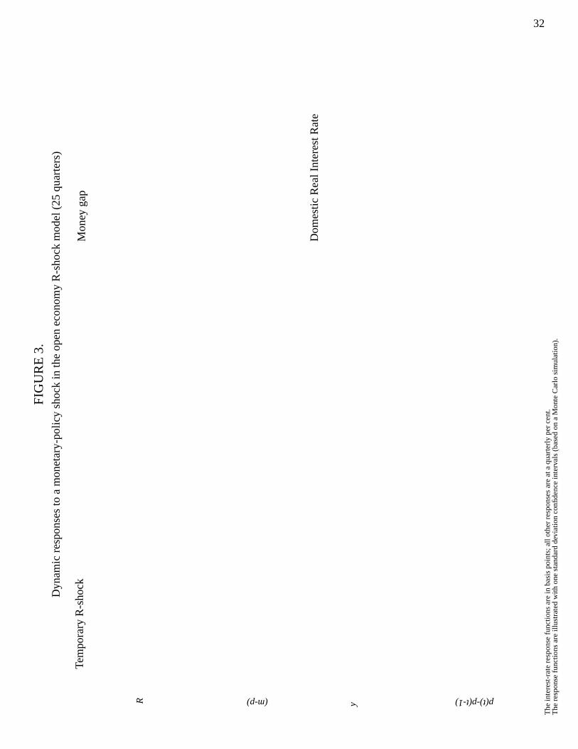
Impulse responses to the R-shock
In response to a positive temporary R-shock (106 basis points), the response of the
overnight interest rate is above zero for about seven quarters (Figure 3, column 1). The
impact response of money is negative and significant. The fall in output is long-lasting: it
takes over 25 quarters for output to return to its pre-shock level (zero). The deviation of
25
domestic real interest rates from equilibrium remains above 20 basis points for over 3
quarters (Figure 3, column 2). This is the source of persistent negative response of output.
In contrast to the M-shock model, the initial response of inflation is positive and
significant. This “price puzzle” is found in several VAR-based studies when the interest
rate is used as the instrument of monetary policy (for example, Sims 1992); it is generally
viewed as a curious result.16 Similar to the M-shock model, the correspondence between
inflation and the money gap remains strong. The long-run demand for money falls initially
with the increase in nominal (and real) interest rates (Figure 3, column 2). This leads to a
positive money gap initially. In order to accommodate the fall in demand, a contraction of
the money supply is required. However, after the fourth quarter, the supply of money
overshoots the long-run demand and the money gap becomes negative. As in the M-shock
models, this long-lasting contraction leads to a fall in the rate of inflation after six quarters.
Overall, the response functions for the R-shock model are consistent with an active-money
view.
16. In comparison, Armour, Engert and Fung (1996) found no evidence of a price puzzle following an over-night interest-rate shock. The R-shock model used in this paper differs from that of Armour, Engert andFung primarily in the measure of the price level: the latter paper measured the price level as the GDP deflatorinstead of the CPI, and this may help account for the different results.
26
7. Conclusions
The empirical results of the M-shock models conform to a monetary-policy shock. A
permanent increase in the nominal stock of M1 generates: a temporary fall in interest
rates, consistent with the liquidity effect; a temporary rise in real output; a permanent
increase in the price level; and a permanent depreciation of the nominal exchange rate.
Previous literature, such as Sims (1986) and Christiano and Eichenbaum (1992), argue
that M1 shocks are poor measures of monetary-policy shocks. This paper suggests that the
conclusions of previous research may be attributable to the identification strategy. In
addition, using a quantity measure of monetary policy and long-run cointegration
restrictions to identify monetary-policy shocks, the M-shock models do not display the
price and exchange-rate puzzles found in several previous VAR-based studies. The R-
shock models yield results that are broadly consistent with previous literature: a temporary
real-interest-rate shock generates a temporary fall in money and output, but prices rise
initially (a “price puzzle”) before eventually declining.
Both the M-shock and R-shock models are consistent with the view that money
plays an active role in the transmission of monetary policy. The slow equilibrium
adjustment of the models implies that monetary policy can have short-run real economic
effects. The similarity between interest-rate dynamics in the two M-shock models
suggests that the central bank manipulates a quantity instrument (such as settlement
balances) in order to attain a particular interest-rate path. Also in the M-shock model,
since the equilibrium adjustment of the nominal exchange rate is faster than the price
level, the real exchange rate overshoots. In the R-shock model, the real interest rate also
overshoots its equilibrium. These overshooting properties suggest that a monetary-policy
shock may have long-lasting output effects.
Although there are considerable differences in the institutional setting and the
implementation of monetary policy across industrialized countries, there is no reason to
believe that the fundamental effects of unanticipated monetary policy are very different.
Future research will examine whether the dynamics of M-shock models are robust across
By multiplying both sides of equation (A.1) by and combining it with equation (3.7),
we obtain
. (A.2)
By definition of the restricted matrix of long-run multipliers (equation (3.9)) equation
(A.2) can be rewritten as
. (A.3)
Combining equations (A.2) and (A.3) gives
. (A.4)
By multiplying both sides of equation (A.4) by their respective transposes and taking the
expectation, we obtain
1. This section is an adaptation of the appendix of King et al. (1991).
∆Xt G L( )et= ∆Xt Φ L( )εt=
Φ L( )Φ01–
G L( )=
Φ0εt et=
L 1=
Φ 1( ) G 1( )Φ0=
εt
Φ 1( )εt G 1( )et=
Φ 1( )εt AΠ 0[ ]εt AΠεtP
= =
AΠεtP
G 1( )et=
34
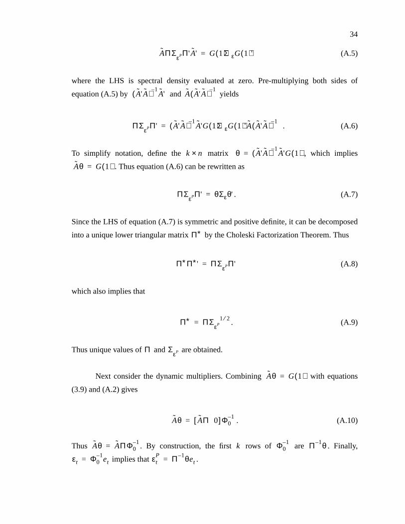
(A.5)
where the LHS is spectral density evaluated at zero. Pre-multiplying both sides of
equation (A.5) by and yields
. (A.6)
To simplify notation, define the matrix , which implies
. Thus equation (A.6) can be rewritten as
. (A.7)
Since the LHS of equation (A.7) is symmetric and positive definite, it can be decomposed
into a unique lower triangular matrix by the Choleski Factorization Theorem. Thus
(A.8)
which also implies that
. (A.9)
Thus unique values of and are obtained.
Next consider the dynamic multipliers. Combining with equations
(3.9) and (A.2) gives
. (A.10)
Thus . By construction, the first rows of are . Finally,
implies that .
AΠΣεPΠ'A'˜ G 1( )ΣεG 1( )'=
A'˜ A( )1–A'˜ A A'˜ A( )
1–
ΠΣεPΠ' A'˜ A( )
1–A'˜ G 1( )ΣεG 1( )'A A'˜ A( )
1–=
k n× θ A'˜ A( )1–A'˜ G 1( )=
Aθ G 1( )=
ΠΣεPΠ' θΣεθ'=
Π∗
Π∗Π∗' ΠΣεPΠ'=
Π∗ ΠΣεP
1 2⁄=
Π ΣεP
Aθ G 1( )=
Aθ AΠ 0[ ]Φ01–
=
Aθ AΠΦ01–
= k Φ01– Π 1– θ
εt Φ01–et= εt
P Π 1– θet=
35
The dynamic multipliers associated with are given by the first columns of
. First, consider the components of the impact matrix . Similar to the matrix of
long-run multipliers, the matrix is partitioned by the number of permanent innovations
in the model. Define the partition of as
(A.11)
where is , is and . Since , the first
columns of are given by
. (A.12)
Consider now the recovery of . Since we have
. (A.13)
Expanding (A.13) and solving for gives . Therefore the dynamic
multipliers for the permanent shocks, , are
. (A.14)
εtP
k
Φ L( ) Φ0
Φ0
Φ0
Φ0 Φk0 Φr0[ ]=
Φk0 n k× Φr0 n r× k r+ n= Φ L( ) G L( )Φ0= k
Φ L( )
G L( )Φk0
Φk0 Φ0εt et=
ΣεΦ0' Φ01– Σe=
Φk0 Φk0' Σε1– Π 1– θΣe=
εtP
Φ L( )Σε1– Π 1– θΣe
36
Appendix 3. Finite-Sample Critical Values
This appendix briefly summarizes the methodology employed in generating the
finite-sample critical values. The non-deterministic parts of the data generated process
(DGP) are drawn from a mean zero 400-period Gaussian distribution with variance one.
The constant term is drawn from a mean ten 400-period Gaussian distribution with
variance one. The analytic asymptotic distribution of the test statistics is approximated by
the Gaussian 400-period random walk (Osterwald-Lenum 1992). For each row, the null
hypothesis of no cointegration is tested ( stochastic trends). By varying , the
number of endogenous variables in the system, critical values are generated row by row.
After replicating this procedure 6,000 times, the asymptotic quantiles are calculated.
There are two differences between the way the finite-sample and asymptotic critical values
are derived. First, and most obvious, the non-deterministic parts of the DGP are drawn
from anf period Gaussian distribution (wheref corresponds to the number of observations
in the estimated models). Second, the quantiles are calculated from 12,000 replications.
The finite-sample critical values of the case with no constant in the DGP but a constant
and a linear shift parameter spanned by the cointegration space (restricted constant) are
presented below.
a. Aside from the inclusion ofD81, this table corresponds to Case 1* in Osterwald-Lenum (1992).
Note:D represents three centered seasonal dummies.
Table 4. Finite-sample Distribution of the Cointegration Test Statistics: Case 1*a
DGP & SM:
-max Trace
90% 95% 99% 90% 95% 99%
1 11.19 13.08 17.34 11.19 13.08 17.34
2 17.94 20.19 24.69 24.45 27.04 32.67
3 24.49 27.02 32.27 41.63 44.93 51.99
4 30.84 33.41 39.19 62.71 66.31 75.05
5 37.37 40.17 45.82 88.39 92.95 102.67
6 43.60 46.66 52.95 117.97 123.51 134.30
7 49.79 52.83 59.93 152.52 158.20 169.79
8 56.23 59.60 66.21 190.56 197.74 210.81
9 62.86 66.23 73.30 233.87 241.75 256.10
10 69.22 72.98 80.57 281.52 289.75 305.55
n r– n
∆Xt Γ1∆Xt 1– … Γk 1– ∆Xt k– 1+ α β' µ0 δ, ,( ) X't 1– 1 D81, ,( )' ΨDt εtεt N 0 I n,( )∼
+ + + + +=
λ
n r–
37
References
Armour, J., W. Engert, and B. S. C. Fung. 1996. “Overnight Rate Innovations as aMeasure of Monetary Policy Shocks.” Working Paper No 96-4. Bank of Canada.
Blanchard, O. and D. Quah. 1989. “The Dynamic Effects of Aggregate Demand andSupply Disturbances.”American Economic Review79, 655-673.
Bernanke, B. 1986. “Alternative Explorations of the Money-Income Correlation.” InRealBusiness Cycles, Real Exchange Rates, and Actual Policies edited by K. Brunner andA. Meltzer, Carnegie-Rochester Conference Series on Public Policy25, 49-99.
Carr, J. and M. Darby. 1981. “The Role of Money Supply Shocks in the Short-RunDemand for Money.”Journal of Monetary Economics8, 183-199.
Christiano, L. and M. Eichenbaum. 1992. “Identification and the Liquidity Effect of aMonetary Policy Shock.” InPolitical Economy, Growth, and Business Cycles, editedby A. Cukierman, L. Hercowitz, and L. Leiderman. Cambridge (MA): MIT Press,335-370.
Cochrane, J. 1994. “Shocks.” Carnegie-Rochester Conference Series on Public Policy41,295-364.
Cooley, T. and S. Leroy. 1985. “Atheoretical Macroeconometrics: A Critique.”Journal ofMonetary Economics16. 283-308.
DeSerres, A. and A. Guay. 1995. “Selection of the Truncation Lag in Structural VARs (orVECMs) with Long-Run Restrictions.” Working Paper No. 95-9. Bank of Canada.
Engle, R. and C. Granger. 1987. “Co-integration and Error Correction: Representation,Estimation, and Testing.”Econometrica55, 251-276.
Faust, J. and E. Leeper. 1994. “When Do Long-Run Identifying Restrictions Give ReliableResults?” International Finance Discussion Papers, Board of Governors of the FederalReserve System, Number 62.
Filosa, R. 1995. “Money Demand Stability and Currency Substitution in Six EuropeanCountries 1980 to 1992).” Working Paper No. 30. Bank for International Settlements.
Fisher, L., P. Fackler, and D. Orden. 1995. “Long-Run Identifying Restrictions for anError-Correction Model of New Zealand Money, Prices and Output.”Journal ofInternational Money and Finance14, 127-147.
Friedman, M. 1956. “The Quantity Theory of Money -- A Restatement.” InStudies in thequantity theory of money edited by M. Friedman, University of Chicago Press, IL.
Friedman, M. 1970. “A Theoretical Framework for Monetary Analysis.” InMiltonFriedman’s Monetary Framework: A Debate with His Critics edited by G. Gordon,University of Chicago Press, IL.
Fung, B. S. C. and R. Gupta. 1994. “Searching for the Liquidity Effect in Canada.”Working Paper No. 94-12. Bank of Canada.
38
Grilli, V. and N. Roubini. 1995. “Liquidity and Exchange Rates: Puzzling Evidence fromthe G-7 Countries.” Working Paper Series S-95-31. New York University.
Hendry, S. 1995. “Long Run Demand for M1.” Working Paper No. 95-11. Bank ofCanada.
Hoffman, D., R. Rasche and M. Tieslau. 1995. “The Stability of Long-Run MoneyDemand in Five industrial Countries.”Journal of Monetary Economics35, 317-339.
Johansen, S. and K. Juselius. 1990. “Maximum Likelihood Estimation and Inference onCointegration -- With Applications to the Demand for Money.”Oxford Bulletin ofEconomics and Statistics52, 169-210.
Johnson, H. 1962. “Monetary Theory and Policy.”American Economic Review52, 335-384.
Keating, J. 1992. “Structural Approaches to Vector Autoregressions.”Federal ReserveBank of St. Louis74, 37-57.
King, R., C. Plosser, J. Stock, and M. Watson. 1987. “Stochastic Trends and EconomicFluctuations.” Working Paper No. 2229. National Bureau of Economic Research.
King, R., C. Plosser, J. Stock, and M. Watson. 1991. “Stochastic Trends and EconomicFluctuations.”American Economic Review81, 819-840.
Laidler, D. 1990. “Taking money seriously and other essays.” Cambridge (MA): MITPress.
Laidler, D. 1994. “Endogenous Buffer-Stock Money.” InCredit, Interest Rate Spreads andthe Monetary Policy Transmission Mechanism. Proceedings of a conference held atthe Bank of Canada (November) 231-258.
Lastrapes, W. and G. Selgin. 1995. “The Liquidity Effect: Identifying Short-Run InterestRate Dynamics Using Long-Run Restrictions.”Journal of Macroeconomics17, 387-404.
Leeper, E. and D. Gordon. 1992. “In Search of the Liquidity Effect.”Journal of MonetaryEconomics29, 341-369.
Lucas, R. 1973. “Some International Evidence on Output-Inflation Tradeoffs.”AmericanEconomic Review63, 326-334.
McKinnon, R. 1982. “Currency Substitution and Instability in the World Dollar Standard.”American Economic Review72, 320-333.
Nelson, C., and C. Plosser. 1982. “Trends and Random Walks in Macroeconomic TimeSeries: Some Evidence and Implications.”Journal of Monetary Economics10, 139-162.
Osterwald-Lenum, M. 1992. “A Note with Quantiles of the Asymptotic Distribution of theMaximum Likelihood Cointegration Rank Test Statistics.”Oxford Bulletin ofEconomics and Statistics54, 461-472.
39
Poloz, S. 1984. “The Transactions Demand for Money in a Two-Currency Economy.”Journal of Monetary Economics14, 241-250.
Poloz, S. 1986. “Currency Substitution and the Precautionary Demand for Money.”Journal of International Money and Finance5, 115-124.
Sargent, T. and N. Wallace. 1975. “‘Rational’ Expectations, the Optimal MonetaryInstrument, and the Optimal Money Supply Rule.”Journal of Political Economy83,241-254.
Sims, C. 1980a. “Comparison of Interwar and Postwar Business Cycles: MonetarismReconsidered.”American Economic Review70, 250-257.
Sims, C. 1980b. “Macroeconomics and Reality.”Econometrica48, 1-48.
Sims, C. 1986. “Are Forecasting Models Usable for Policy Analysis?” Federal ReserveBank of MinneapolisQuarterly Review10, 2-16.
Sims, C. 1992. “Interpreting the Macroeconomic Time Series Facts: The Effects ofMonetary Policy.”European Economic Review36, 975-1000.
Stock, J. and M. Watson. 1993. “A Simple Estimator of Cointegrating Vectors in HigherOrder Integrated Systems.”Econometrica61, 783-820.