+ All Categories
Home > Documents > Intersymbol Interference (ISI) · Symbol rates for ISI free reception Suppose that the ISI free...

Intersymbol Interference (ISI) · Symbol rates for ISI free reception Suppose that the ISI free...

Date post: 19-Mar-2020
Category:
Upload: others
View: 21 times
Download: 0 times
Share this document with a friend
6
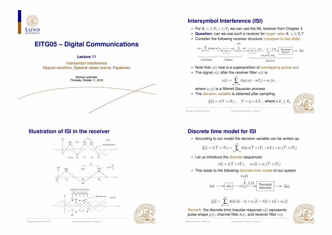
EITG05 – Digital Communications Lecture 11 Intersymbol Interference Nyquist condition, Spectral raised cosine, Equalizers Michael Lentmaier Thursday, October 11, 2018 Intersymbol Interference (ISI) For R s = 1/T s < 1/T u we can use the ML receiver from Chapter 4 Question: can we use such a receiver for larger rates R s 1/T u ? Consider the following receiver structure (compare to last slide) h(t) m[i] ^ + t=t +LT +iT 0 s s Threshold detector [i] ξ s A[n]g(t-nT ) n= 8 v(t) Channel Transmitter w(t) z(t) s(t) = 8 r(t) y(t) Receiver Note that z(t) now is a superposition of overlapping pulses u(t) The signal y(t) after the receiver filter v(t) is y(t)= n=A[n] x(t nT s )+ w c (t) , where w c (t) is a filtered Gaussian process The decision variable is obtained after sampling ξ [i]= y(T + iT s ) , T = t 0 + LT s , where LT s T u Michael Lentmaier, Fall 2018 Digital Communications: Lecture 11 Illustration of ISI in the receiver ξ[0] ξ[1] [3] ξ [2] ξ T s T =T u s 2T s 3T s 4T s 5T s T =T u s y(t) Individual pulses t 0 ξ [0] ξ [1] [2] ξ T s T s 2 s T 3T s 2T s T s 2 T = u y(t) t 2T s ξ [0] ξ [1] [2] ξ [3] ξ ξ [4] s T s T s T s T T =2T u s ISI ISI . . . . . . t Message term Michael Lentmaier, Fall 2018 Digital Communications: Lecture 11 Discrete time model for ISI According to our model the decision variable can be written as ξ [i]= y(T + iT s )= n=A[n] x(T + iT s nT s )+ w c (T + iT s ) Let us introduce the discrete sequences x[i]= x(T + iT s ) , w c [i]= w c (T + iT s ) This leads to the following discrete-time model of our system [i] ξ + w [i] c x[i] Threshold detection m[i] ^ A[i] ξ [i]= n=A[n] x[i n]+ w c [i]= A[i] x[i]+ w c [i] Remark: the discrete-time impulse response x[i] represents pulse shape g(t), channel filter h(t), and receiver filter v(t) Michael Lentmaier, Fall 2018 Digital Communications: Lecture 11
Transcript

EITG05 – Digital Communications

Lecture 11

Intersymbol InterferenceNyquist condition, Spectral raised cosine, Equalizers

Michael LentmaierThursday, October 11, 2018

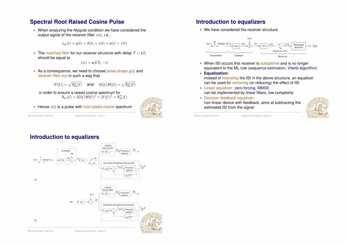
Intersymbol Interference (ISI)� For Rs = 1/Ts < 1/Tu we can use the ML receiver from Chapter 4� Question: can we use such a receiver for larger rates Rs ≥ 1/Tu?� Consider the following receiver structure (compare to last slide)

h(t) m[i]^+

t=t +LT +iT0 s s

Thresholddetector

[i]ξsA[n]g(t-nT )n= 8 v(t)

ChannelTransmitter

w(t)

z(t)s(t) = ∑

8

r(t) y(t)

Receiver

� Note that z(t) now is a superposition of overlapping pulses u(t)� The signal y(t) after the receiver filter v(t) is

y(t) =∞

∑n=−∞

A[n]x(t−nTs)+wc(t) ,

where wc(t) is a filtered Gaussian process� The decision variable is obtained after sampling

ξ [i] = y(T + iTs) , T = t0 +LTs , where LTs ≥ Tu

Michael Lentmaier, Fall 2018 Digital Communications: Lecture 11

Illustration of ISI in the receiver

ξ [0] ξ [1] [3]ξ[2]ξ

TsT =Tu s

2Ts 3Ts 4Ts 5TsT =Tu s

y(t)

Individual pulses

t0

ξ [0] ξ [1] [2]ξ

Ts

Ts2 sT 3Ts2Ts

Ts2

T =uy(t)

t

2Ts

ξ [0] ξ [1] [2]ξ [3]ξ ξ [4]

sT sT sTsT

T =2Tu s

ISI

ISI

. . . . . .

t

Message term

Michael Lentmaier, Fall 2018 Digital Communications: Lecture 11

Discrete time model for ISI� According to our model the decision variable can be written as

ξ [i] = y(T + iTs) =∞

∑n=−∞

A[n]x(T + iTs −nTs)+wc(T + iTs)

� Let us introduce the discrete sequences

x[i] = x(T + iTs) , wc[i] = wc(T + iTs)

� This leads to the following discrete-time model of our system

[i]ξ+

w [i]c

x[i] Thresholddetection m[i]^A[i]

ξ [i] =∞

∑n=−∞

A[n]x[i−n]+wc[i] = A[i] ∗ x[i]+wc[i]

Remark: the discrete-time impulse response x[i] representspulse shape g(t), channel filter h(t), and receiver filter v(t)

Michael Lentmaier, Fall 2018 Digital Communications: Lecture 11

Example 6.1The transmitted sequence of amplitudes A[i] is given as,

A[i]

1

1 5 8 9i

Calculate, and plot, the sequence of decision variables ξ[i] in Figure 6.2, for 0 ≤ i ≤ 8,in the noiseless case (i.e. w(t) = 0) if t0 = 0 and if the output pulse x(t) is:

Ts 2Ts

x0

2Ts 4TsTs

x0

x(t)

0t

x(t)

t

i) L=1 and x(t) as below. ii) L=2 and x(t) as below.

� i) ξ [i] = x0 A[i] ii) ξ [i] = x02 A[i+1]+ x0 A[i]+ x0

2 A[i−1]ξ [i]

x0

-x 0

i1 5 6 8

Michael Lentmaier, Fall 2018 Digital Communications: Lecture 11

How much ISI can we tolerate?� We can divide the decision variable ξ [i] into a desired term

(message) and an undesired term (interference plus noise)

ξ [i] = A[i]x[0]

︸ ︷︷ ︸message

+∞

∑n=−∞

n�=i

A[n]x[i−n]

︸ ︷︷ ︸ISI

+wc[i]

︸︷︷︸noise

� The influence of ISI depends on its relative strength

ISI-freenoise-freevalueA[i]x[0]

ξ [i]

Noisemargin

Worstcase:

ISIwc

Worstcase:

ISIwc

Noisemargin

Noise marginwithout ISI = D/2

Decision boundaries

- +

Michael Lentmaier, Fall 2018 Digital Communications: Lecture 11

Worst case ISI� The ISI term can be written as

ISI =∞

∑n=−∞

n�=i

A[n]x[i−n] =∞

∑n=−∞

n�=0

A[i−n]x[n]

� Question: when does this term become largest?� For symmetric M-ary PAM we have max |A[i]|= M−1 and get

ISI+wc = max(ISI) =∞

∑n=−∞

n�=0

max(A[i−n]x[n]) = (M−1)∞

∑n=−∞

n�=0

|x[n] |

� Similarly, the worst case minimal ISI becomes

ISI−wc = min(ISI) =−(M−1)∞

∑n=−∞

n�=0

|x[n] |

Observe: the worst case ISI occurs for a information sequenceA[i] consisting of a particular pattern of ±(M−1) values

Michael Lentmaier, Fall 2018 Digital Communications: Lecture 11

Condition for ISI free reception� Let us assume that x[i] satisfies the following condition:

x[i] = x(T + iTs) = x0 δ [i] =

{x0 if i = 00 if i �= 0

� Then

ξ [i] =∞

∑n=−∞

A[n]x[i−n]+wc[i] = A[i]x[0] +wc[i]

� Otherwise there always will exist some non-zero ISI term� For this reason we are interested in signals

x(t) = g(t) ∗ h(t) ∗ v(t)

for which the above condition is satisfied

Which parts of x(t) can we influence?

Michael Lentmaier, Fall 2018 Digital Communications: Lecture 11

Symbol rates for ISI free reception� Suppose that the ISI free condition is satisfied for symbol rate R∗

s

� Then it will be satisfied for rates

Rs =R∗

s

�, �= 1,2,3, . . .

Example 6.6:Consider the overall pulse shape x(t) below, and T = 4/7200.

x0

72004

72001

72008

t [s]

x(t)

Assume the bitrate 14400 [b/s] and 16-ary PAM signaling. Does ISI occur in thereceiver?

Michael Lentmaier, Fall 2018 Digital Communications: Lecture 11

Representation in frequency domain� The discrete sequence x[i] can be obtained by sampling a

non-causal pulse xnc(t) at times iTs,

x[i] = xnc(iTs) , where xnc(t) = x(T + t) ,

� The Fourier transform X (ν) of x[i] can then be expressed interms of the Fourier transform Xnc(f ) of the signal xnc(t):

X (ν) =∞

∑n=−∞

x[n]e− j2π ν n =1Ts

∑n=−∞

Xnc

(ν −n

Ts

),

where

Xnc(f ) =∫ ∞

−∞xnc(t)e−j2π f t dt = G(f )H(f )V(f )e+j2π f T

Observe: the spectrum of the sampled sequence x[i] consistsof the periodically repeated spectrum of the continuous signal

Michael Lentmaier, Fall 2018 Digital Communications: Lecture 11

Nyquist condition in frequency domain� Let us now formulate the ISI free condition in frequency domain:

x[i] = x0 δ [i] ⇒X (ν) = F{x[i]}= x0 ∀ν

� Choosing ν = f Ts this leads to the equivalent Nyquist condition

X (f Ts)

Rs=

∑n=−∞

Xnc(f −nRs) =x0

Rs, Rs =

1Ts

� Let Wlp denote the baseband bandwidth of xnc(t),

Xnc(f ) = 0, |f |> Wlp

� Then ISI always will be present if the symbol rate satisfies

Rs > 2Wlp

(non-overlapping spectrum cannot add up to a constant)� If we have Rs ≤ 2Wlp:

ISI-free reception is possible if Xnc(f ) has a proper shape

Michael Lentmaier, Fall 2018 Digital Communications: Lecture 11

Example 6.7Assume that Xnc(f) is given below.

X (f)nc

4000 4000

A

f [Hz]0

a) Sketch the left hand side of (6.33), ∞n=−∞ Xnc(f−nRs), if Rs = 12000 symbols

per second.

b) Does ISI occur in the receiver?

What happens if Rs = 8000?

And Rs = 4000?

Michael Lentmaier, Fall 2018 Digital Communications: Lecture 11

Example 6.8Assume that Xnc(f) is,

4000

X (f)nc

4000f [Hz]

0

A

A = x0Ts.Show that there is no ISI if the symbol rate is Rs = 8000 [symbol/s].

Solution:

X (f-n8000)ncn= 8

8

800016000 4000 8000 160004000 24000f [Hz]

A

0

Since

n=−∞Xnc(f − n8000) = x0/Rs, for all f , there is no ISI in the receiver.

Michael Lentmaier, Fall 2018 Digital Communications: Lecture 11

Ideal Nyquist pulse� The maximum possible signaling rate for ISI-free reception is

Rnyq = Rs =1Ts

= 2Wlp (Nyquist rate)

� With ideal Nyquist signaling, the bandwidth efficiency is

ρnyq =Rb

Wlp=

Rnyq log2(M)

Rnyq/2= 2 log2 M = 2k [bps/Hz]

� The ideal Nyquist pulse must have rectangular spectrum

Xnc(f ) =

{x0/Rnyq , if |f | ≤ Rnyq/20 , else

⇒ xnc(t) = x0sin(π Rnyq t)

π Rnyq t

x (t)nc

x0

X (f)nc

x0/Rnyq

R nyq/2R nyq/2

nyqR1

nyqR1

= -T s nyqR1 = Ts

b)

tf [Hz]

a)

Michael Lentmaier, Fall 2018 Digital Communications: Lecture 11

Some comments on bandwidth� Remember: in Chapter 2 we have seen that strictly band-limited

signals always have to be unlimited in time� In practice we have to find compromises, which was leading to

different definitions of bandwidth for time-limited signals

Pulse shape Wlobe % power W90 W99 W99.9 Asymptoticin Wlobe decay

rec 2/T 90.3 1.70/T 20.6/T 204/T f−2

tri 4/T 99.7 1.70/T 2.60/T 6.24/T f−4

hcs 3/T 99.5 1.56/T 2.36/T 5.48/T f−4

rc 4/T 99.95 1.90/T 2.82/T 3.46/T f−6

Nyquist Rs 100 0.9Rs 0.99Rs 0.999Rs ideal

� We can see that time-limited signals need at least about twicethe Nyquist bandwidth

� For OFDM with many sub-carriers N this is negligible (why?)� For single-carrier systems, some close-to-Nyquist pulses

are typically used in practice

Michael Lentmaier, Fall 2018 Digital Communications: Lecture 11

Spectral Raised Cosine Pulses� The spectral raised cosine pulse shape is defined by the

following spectrumX (f)nc

x T0 s

Ts

1Ts

1Ts21

Ts21

β=1

β=0

Rs2pW =(1+ )β

0f

� The name refers to the way the shape is composed

Xnc(f ) =

x0 Ts , 0 ≤ |f | ≤ 1−β2Ts

x0 Ts2

[1+ cos

(π|f |Ts

β − π2 · 1−β

β

)], 1−β

2Ts≤ |f | ≤ Wlp

0 |f |> Wlp

where Wlp =1+β2Ts

= (1+β )Rs

2, 0 ≤ β ≤ 1

Michael Lentmaier, Fall 2018 Digital Communications: Lecture 11

Spectral Raised Cosine Pulses� The parameter β , 0 ≤ β ≤ 1, is called the rolloff factor and can be

used to smoothly control the bandwidth efficiency

ρsrc =Rb

Wlp=

Rs log2 M(1+β )Rs/2

=2 log2 M

1+β=

2k1+β

� In time domain the signal can be expressed as

xnc(t) = x0sin(πt/Ts)

πt/Ts· cos(πβ t/Ts)

1− (2β t/Ts)2 , −∞ ≤ t ≤ ∞

x (t)nc

β=1

β=0

Ts Ts2 Ts3 Ts4 Ts5 Ts6

Ts-4 Ts-2

Ts-5 Ts-3 Ts-

t

� Larger rolloff factors β ⇒ faster amplitude decay of xnc(t)

Michael Lentmaier, Fall 2018 Digital Communications: Lecture 11

Spectral Raised Cosine Pulses

-5 -4 -3 -2 -1 0 1 2 3 4 5

t/Ts

-0.4

-0.2

0

0.2

0.4

0.6

0.8

1

Michael Lentmaier, Fall 2018 Digital Communications: Lecture 11

Signaling with overlapping pulses: β = 1

1 2 3 4 5 6 7

t/Ts

-1

-0.5

0.5

1

1 2 3 4 5 6 7

t/Ts

-1

-0.5

0.5

1

Michael Lentmaier, Fall 2018 Digital Communications: Lecture 11

Signaling with overlapping pulses: β = 0

1 2 3 4 5 6 7

t/Ts

-1

-0.5

0.5

1

1 2 3 4 5 6 7

t/Ts

-1

1

Michael Lentmaier, Fall 2018 Digital Communications: Lecture 11

Spectral Root Raised Cosine Pulse� When analyzing the Nyquist condition we have considered the

output signal of the receiver filter v(t), i.e.,

xnc(t) = g(t) ∗ h(t) ∗ v(t) = u(t) ∗ v(t)

� The matched filter for our receiver structure with delay T = LTsshould be equal to

v(t) = u(LTs − t)

� As a consequence, we need to choose pulse shape g(t) andreceiver filter v(t) in such a way that

|V(f )|=√

Xrcnc(f ) and |G(f )H(f )|=

√Xrc

nc(f )

in order to ensure a raised cosine spectrum forXnc(f ) = |G(f )H(f )|2 = |V(f )|2 = Xrc

nc(f )

� Hence v(t) is a pulse with root-raised cosine spectrum

Michael Lentmaier, Fall 2018 Digital Communications: Lecture 11

Introduction to equalizers� We have considered the receiver structure

h(t) m[i]^+

t=t +LT +iT0 s s

Thresholddetector

[i]ξsA[n]g(t-nT )n= 8 v(t)

ChannelTransmitter

w(t)

z(t)s(t) = ∑

8

r(t) y(t)

Receiver

� When ISI occurs this receiver is suboptimal and is no longerequivalent to the ML rule (sequence estimation, Viterbi algorithm)

� Equalization:instead of tolerating the ISI in the above structure, an equalizercan be used for removing (or reducing) the effect of ISI

� Linear equalizer: zero-forcing, MMSEcan be implemented by linear filters, low complexity

� Decision feedback equalizer:non-linear device with feedback, aims at subtracting theestimated ISI from the signal

Michael Lentmaier, Fall 2018 Digital Communications: Lecture 11

Introduction to equalizers

s(t) = Σ A[n]g(t-nT )

8

n=-

8 H(f) v(t)z(t) r(t) y[i]

w(t)CHANNEL

t=T 0+iT s

a)

Adfe [i]~

DECISION-FEEDBACK EQUALIZER

pff[i]Thresholddetector

pfb[i]

p[i]

LINEAREQUALIZER

A[i]~

Thresholddetector

A[i]^

Adfe [i]^

Adfe [i]~

DECISION-FEEDBACK EQUALIZER

pff[i]Thresholddetector

pfb[i]

p[i]

LINEAREQUALIZER

A[i]~

Thresholddetector

A[i]^

Adfe [i]^

x[i]A[i]y[i]

wc[i]

b)

s

Michael Lentmaier, Fall 2018 Digital Communications: Lecture 11


Recommended