Frenkel/Razin/Sadka:cgInt'l Taxation--Chapter 4

October 23, 1990

CHAPTER 4: EQUIVALENCE RELATIONS IN TAXATION*

4.1 Introduction

This chapter is about equivalence relations among different

combinations of fiscal instruments. Taxes themselves may vary in many

apparently significant respects, such as who pays them, what country

collects them, when the taxes are collected, and whether the fiscal

instruments are even thought of as taxes. Yet many of these differences

vanish with the households and firms. The resulting equivalences have an

important bearing on the design and effectiveness of tax policy. They

suggest that a given objective may be accomplished in a variety of different

ways, some perhaps more feasible or politically acceptable than others.

Another implications, however, is that a tax policy may be subverted by the

failure to coordinate such equivalent channels. These implications can be

of considerable economic significance, and there is ample evidence that

they, as well as the equivalences themselves, are of prime relevance for

policymaking.

Based on Alan Auerbach, Jacob Frenkel, and Assaf Razin, "Notes on*

International Taxation," February 1989. We are indebted to Alan Auerbachfor agreeing to include this chapter in the book.

- 2 -

For example, one fundamental equivalence discussed below is of

combinations of trade-based (border) taxes on exports and imports and

domestic taxes on production and consumption. A second equivalence concerns

direct and indirect taxation. As Anthony Atkinson (1977) puts it, direct

taxes are taxes that can be based on specific characteristics of individuals

and households (e.g., marital status, number of dependents, age, etc.) or

businesses (e.g., type of industry). The main forms of direct taxes are

personal and corporate income taxes, wealth taxes and inheritance taxes.

Indirect taxes are taxes based on transactions such as consumption, exports

or imports. As we argue below, the relevance of these equivalences can be

demonstrated using the economic integration of the countries of the European

Community (EC).

Among the goals of the 1992 process of economic integration in Europe

is a harmonization of national tax systems, aimed at eliminating the adverse

incentives for the movement of capital, goods and production activity that

may derive from the conflicting national objectives of independently

designed national tax systems.

Economic integration obviously requires limits on the ability of

countries to tax or subsidize exports or imports within the integrated

community. In addition, in recognition of the relevance of domestic

taxation to export and import incentives, two types of domestic indirect

taxation are dealt with in the harmonization provisions. As indicated in

Chapter 2, an important indirect tax used in the EC is the value-added

tax (VAT) that applies to the domestic consumption of goods and services.

As demonstrated in Table 2.2, the coverage, rates and method of calculation

- 3 -

of such taxes vary extensively among the member countries. The difference

in tax rates gives rise to incentives to move reported sales from high-tax

to low-tax countries. Because of differences in tax base definition, some

sales across national borders may be taxed in more than one country. The

harmonization proposals would attack these problems by reducing the extent

of tax rate variation and standardizing the tax base definition. In

addition, the excise duties currently levied at very different rates among

countries on specific commodities such as alcoholic beverages, cigarettes

and gasoline would be entirely harmonized at uniform rates of tax for each

commodity.

The apparent motivation for these provisions is that they will

facilitate the elimination of fiscal frontiers within the EC. This

exclusive focus on indirect taxation is also found in the provisions of GATT

which restrict tax-based trade barriers. The discussion in this chapter

implies, however, that there is little theoretical basis for such an

approach. Just as domestic and trade-based indirect taxes have similar

effects that require coordination, so too do direct and indirect taxes.

To provide the intuition for certain tax equivalences, we begin with a

simple model in which many different types of tax policy are assumed to be

the same and then show the conditions under which some of these very basic

equivalences carry over to much more refined models which are better suited

for guiding policy actions.

- 4 -

4.2 One-Period Model

Consider a one-period model of a small open economy with a single

representative consumer. The country produces two goods in domestically-

owned industries and both goods are consumed domestically. One good, X,

is exported, as well as being domestically consumed. The other good, M,

is imported, as well as being domestically produced. Each good is produced

using two factors of production, labor, L, and capital, K. Let C bei

the domestic consumption of good i; L and K the levels of labor andi i

capital allocated to industry i, respectively; w and r the factor

returns of labor and capital, respectively; and B the pure profitsi

generated for the household sector by industry i, (i=X,M). Let the world

price of the export good be normalized to unity, with the relative world

price of the imported good equal to p . In the absence of taxes, theM

household's budget constraint is:

C + p C = wL + wL + rK + rK + B + B . (4.1)X M M X M X M X M

Equation (4.1) states, simply, that spending equals income.

This household's budget constraint may be derived in an alternative way

via the production and trade sectors of the economy. Starting with the

production sector accounts, which require that production, in sector i, Z , i

equal factor payments plus profits, we obtain:

p Z = wL + rK + B , (i = X, M). (4.2)i i i i i

- 5 -

To this, we add the requirement that trade must be balanced; that is,

exports must equal imports:

p (C - Z ) = Z - C . (4.3)M M M X X

Equation (4.3) is a requirement imposed by the model's single period

assumption. No country will be willing to "lend" goods to the rest of the

world by running a trade surplus, since there will be no subsequent period

in which the debt can be repaid via a trade deficit. Using equation (4.2)

in equation (4.3) yields equation (4.1), which can be then viewed as the

overall budget constraint of the economy.

Let us now introduce to this model, a variety of taxes including

consumption taxes, income taxes and trade taxes. In practice, consumption

taxes may take a variety of forms, including retail sales taxes and value-

added taxes on consumption goods. In this simple model, with no

intermediate production, the two types of taxes are identical. One could

also impose a direct consumption tax at the household level. Although there

has been considerable theoretical discussion of personal consumption taxes,

no country has yet adopted such a tax.

4.2.1 Simple Equivalences

Let the tax on good i be expressed as a fraction J ofi

the producer price. (A basic and familiar feature concerning excise taxes

is that it is irrelevant whether the tax is paid by the producer or the

consumer.) The tax appears on the left-hand side of the budget constraint

- 6 -

(4.1), with the export good's domestic consumer price becoming 1 + J andX

the import good's domestic consumer price becoming (1+J )p ); the producerM M

domestic prices are p / 1 and p , respectively.X M

The first very simple equivalence to note is that the taxes

could also be expressed as fractions (J , i = X, M) of the consumeri'

prices, in which case the consumer prices would become p /(1-J' ). Thisi i

distinction is between a tax, J, that has a tax-exclusive base and one,

J', that has a tax-inclusive base. If r' = J/(1+J), then the two taxes

have identical effects on the consumer and producer and provide the same

revenue to the government. Yet, when tax rates get reasonably high, the

nominal difference between tax-exclusive and tax-inclusive rates becomes

quite substantial. A tax-inclusive rate of 50 percent, for example, is

equivalent to a tax-exclusive rate of 100 percent.

Consider now income taxes on profits and returns to labor and

capital. Rather than raising consumer prices, these taxes reduce the

resources available to consume. In practice, such taxes are assessed both

directly and indirectly. There are individual and business income taxes,

but also payroll taxes, for example. By the national income identity, a

uniform value-added tax on all production is simply an indirect tax on

domestic factor incomes, both payrolls and returns to capital and profits.

One may note, as in the case of consumption taxes, that it

does not matter whether the supplier of a factor, in this case the

household, or the user, in this case the firm, must actually remit the tax.

A factor tax introduced in equation (4.2) or (4.1) has the same effect. The

same point holds in regard to tax-exclusive versus tax-inclusive tax bases.

- 7 -

One also may observe from inspection of (4.1) that a uniform tax on income

is equivalent to uniform tax on consumption. Each tax reduces real income.

Imposition of tax-inclusive consumption tax at rate J divides the left-

hand side of (4.1) by the factor (1-J) while a tax-inclusive income tax (the

way an income tax base is normally defined) at the same rate multiplies the

right-hand side of (4.1) by (1-J). Since dividing one side of an equation

by a certain factor is equivalent to multiplying the other side of the same

factor, the equivalence between a uniform consumption tax and a uniform

income tax is established in a one-period model.

Despite their simplicity, these basic equivalences are useful

in understanding the potential effects of various policies. For example,

the EC tax harmonization provisions discussed above would narrow differences

in rates of VAT among member countries, but these provisions say nothing

about income taxes. Yet our results suggest that a uniform consumption tax

or any type of uniform income tax would be equivalent to a uniform VAT.

Thus, a country with a VAT deemed too high could accede to the provisions of

the harmonization process by lowering its VAT and raising other domestic

taxes, with no resulting impact on its own citizens and, a fortiori, on the

citizens of other countries either. One must conclude that either these

proposals have not taken adequate account of simple equivalences or that the

simple equivalences may break down in more complicated situations, a

possibility we explore below.

- 8 -

4.2.2. International Trade Equivalences

We turn now to taxes explicitly related to international

trade. We say explicitly, of course, because an obvious theme of this

chapter is that one must recognize the equivalences that make some policies,

not specifically targeted at trade, perfect substitutes for others that are.

Tax-based trade policies may involve border taxes, such as

tariffs on imports or export subsidies, but may also be industry-specific

taxes aimed, for example, at making trade-sensitive industries more

competitive. It is well known that quantity restrictions may in some cases

be used to replicate the effects on trade-based taxes. The most familiar

case is the use of import quotas instead of tariffs. Other alternatives to

explicit tax policies are discussed further below.

The first equivalence we note among trade-based tax policies

is between taxes on exports and taxes on imports. One might imagine that

these policies would work in opposite directions, since the first appears to

encourage a trade deficit (a decline in exports not of imports) while the

second to discourage one. However, it must be remembered that this one-

period model requires balanced trade. Hence, there can be no trade deficit

or surplus; only the level of balanced trade may be influenced. Once this

is recognized, the equivalence of these two policies can be more rapidly

understood; each policy discourages trade by driving a wedge between the

buyer's and seller's prices of one of the traded goods. This is the well-

known Lerner's Symmetry Proposition.

Algebraically, the equivalence is straightforward. An import

tax at a tax-exclusive rate of J causes the domestic price of the imported

- 9 -

good to equal the world price, p , multiplied by the factor 1 + J. NoteM

that since the import tax does not apply to the domestic producer, then

p (1 + J) is the domestic price not only for the consumer but rather alsoM

for the domestic producer. Denoting by w and r the equilibrium factor

returns to labor and capital, respectively, the 4-tuple

(p (1 + J), 1, w, r) is an equilibrium domestic price vector with an importM

tax at a tax-exclusive rate of J. On the other hand, an export tax at the

same tax-exclusive rate of J causes the exporting firm to receive only

1/(1 + J) for every unit of the export good sold at the export price of

one. The rest, J/(1 + J), equals the tax exporters must pay, which is the

tax rate times the net price received, 1/(1 + J). Note that 1/(1 + J)

becomes also the domestic price of the export good, as an exporter can

either sell domestically or abroad and must therefore receive the same net

price at home and abroad. Multiplying the price vector (4.4) by 1/(1 + J),

we obtain another price vector

(p , 1/(1 + J), w', r') (4.5)M

where w = w/(1 + J) and r = r/(1 + J). Notice that the price vectors' '

(4.4) and (4.5) represent the same relative prices. As only relative prices

matter for economic behavior, the two price vectors, (4.4) and (4.5),

support the same equilibrium allocation. Put it differently, multiplying

p on the left-hand side of the household's budget constraint by 1 + J M

(an import tax) is equivalent to multiplying all other prices in that

equation (and the profits B and B ) by 1/(1 + J) (an export tax). M X

- 10 -

Thus, the equivalence between an import tax at a tax-exclusive rate of J

(which generates the equilibrium price vector (4.4)) and an export tax at

the same tax-exclusive rate of J (which generates the equilibrium price

vector (4.5)) is established.

It is important to point out that this symmetry of trade

taxes makes no assumption about whether the taxing country is small or

large, i.e., whether its policies can affect the relative world price of the

two goods. The equivalence indicates that these two policies are really

one.

4.2.3. Equivalences Between Trade and Domestic Policies

The next class of policy equivalences we note is between

trade policies and combinations of domestic policies. We have already shown

that an import tariff at a tax-exclusive rate J causes the domestic price

of the imported good to equal the world price, p , multiplied by theM

factor 1 + J. We also noted that p (1 + J) is the domestic price for bothM

the consumer and the producer. If, instead of an import tax at a tax-

exclusive rate of J the government imposes an excise (consumption) tax at

the same tax-exclusive rate of J, then the consumer price of the import

good becomes p (1 + J), but the producer price remains the world price ofM

p . However, the producer will be indifferent between the import tax whichM

generates a producer price of p (1 + J) and the excise tax (whichM

generates a producer price of only p ), if the excise tax is accompanied byM

a subsidy at a rate J to domestic production which raises the price for

him back to p (1 + J). An immediate implication is that one cannot controlM

- 11 -

tax-based trade barriers without also controlling domestic taxes, and that

controlling only domestic sales or consumption taxes alone is still not

enough. It is possible to convert a perfectly domestic sales tax into an

import tariff by subsidizing domestic production of the commodity in

question at the rate of consumption tax already in place.

4.3 Multiperiod Model

Many of the equivalences just demonstrated hold in very general models.

Even those that do not may "break down" in much more limited ways than one

might think. Furthermore, the conditions under which such equivalences do

fail provide insight into the channels through which different tax policies

operate. Perhaps the most important extension of the simple model we have

used in the addition of several periods during which households may produce

and consume. This permits the appearance of saving, investment and

imbalances of both the government and trade accounts, the "two deficits."

In fact, one may go quite far toward such a model simply by

reinterpreting the previous one. Consider, once again, the basic model of

equations (4.1)-(4.3). We originally interpreted this as a one-period

model, with capital and labor as primary factors supplied to the production

process and p , w, and r the one-period relative prices of imports,M

labor and capital. Suppose, instead, that we wished to consider a

multiperiod economy. What would the budget constraint of a household

choosing consumption and labor supply over several periods look like? From

Chapter 3, we know that the household planning no bequests would equate the

present value of its lifetime consumption to the present value of its

- 12 -

lifetime labor income plus the initial value of its tangible wealth. What

is this initial wealth? It equals the present value of all future profits

plus the value of the initial capital stock. The value of the initial

capital stock, in turn, may also be expressed as the present value of all

future earnings on that capital. Thus, we may replace expression (4.1) with

PV(C + P C ) = PV(wL + wL ) + PV(rK + rK ) + PV(B + B ), (4.6)X M M X M X M X M

where PV( ) represents the present value of a future stream rather than a

single period quantity, K is the initial capital stock of industry i,i

and L and B are the flows of industry i's labor input and profits ini i

period i.

In (4.6), we have made the transition to a multiperiod budget

constraint. Note that this budget constraint no longer implies that income

equal consumption in any given period, only that lifetime income (from labor

plus initial wealth) equal lifetime consumption, in present value. Thus,

there may be saving in some periods and dissaving in others.

Similar adjustments are needed to equations (4.2) and (4.3) to complete

the transition to a multiperiod model. Just as a household need not balance

its budget in any given year, a country need not have balanced trade in any

given year. Over the entire horizon of the model, however, trade must be

balanced in present value, following the argument used above for balance in

the one-period model. That is, each country will give up no more goods and

services, in present value, than it receives. The dates of these matching

exports and imports may be different, of course, and this is what gives rise

to single-period trade deficits and surpluses. Thus, equation (4.3)

becomes:

- 13 -

PV[p [C - Z )] = PV[Z - C ] . (4.7)M M M X X

The last equation in need of reinterpretation is (4.2). The natural

analogue in the multiperiod context is:

PV(p Z ) = PV(wL ) + PV(rK ) + PV(B ) i = X, M, (4.8)i i i i i

which says that the present value of output in each industry equals the

present value of the streams of payments to labor and profits plus the

payments to the initial capital stock. However, this condition requires

further explanation, since one might expect returns to all capital over

time, and not just the initial capital stock, to appear on the right-hand

side of the expression.

The explanation is that new investment and its returns are subsumed by

the "final form" relationship between final outputs and primary inputs given

in (4.8). Put it differently, Z is interpreted as the output that isi

available for final uses outside the production sector, i.e., Z is outputi

that is available for either domestic consumption or exports. One may think

of capital goods produced after the initial date and then used in production

as intermediate goods. Normal production relations represent each stage of

production. In a two-period model, for example, we would depict first-

period capital and consumption as being produced by initial capital and

first-period labor, and second-period consumption as being produced by

initial capital plus capital produced during the first period, and second-

period labor. Inserting the first-period production relation into the

- 14 -

second-period production relation allows us to eliminate first-period

capital from the equation, giving us a single "final form" relating each

period's consumption to each period's labor input and the initial stock of

capital. This approach may be applied recursively in the same manner for

multiperiod models, leading to the type of relationship given in (4.8). In

fact, if the capital goods produced in one industry are used in the other,

then (4.8) does not hold for each industry separately; only when the two

conditions are summed together. This is still consistent with conditions

(4.6) and (4.7).

Given the similarity of the multiperiod model (4.6)-(4.8) and the

single-period model (4.1)-(4.3), it is not surprising that several of the

one-period equivalences carry over to the multiperiod model. First, a

permanent tax on consumption is equivalent to a permanent tax on labor

income plus profits plus the returns to the initial capital stock. A

permanent consumption tax at a tax-exclusive rate of J causes expression

(4.6) to become

PV[(1+J)(C +p C )] = PV(wL +wL ) + PV(rK +rK ) + PV(B +B ) . (4.9)X M M X M X M X M

Multiplying this equation by 1-J' / 1/(1+J), we obtain:

PV(C +P C ) = PV[(wL +wL )(1-J')] + PV[(rK +rK )(1-J')]X M M X M K M

+ PV[(B + B )(1-J')]. (4.10)M X

- 15 -

Equation (4.10) is obtained from (4.6) when a permanent tax at a tax-

inclusive rate of J' is imposed on labor income plus profits plus the

returns to the initial stock of capital. Thus, the equivalence between the

latter tax and a consumption tax is established. Clearly, this equivalence

holds only if the tax rates are constant over time, so that the tax terms

can be taken outside the present value operators PV ( ). One may be tempted

to interpret this result as showing that consumption taxes and income taxes

are equivalent in multiperiod models with saving, but it is important to

recognize that the type of income tax imposed here is not the income tax as

normally conceived. The tax here is on wage income plus capital income

attributable to initial wealth. It excludes from the tax base the income

attributable to capital generated by saving done during the model's periods.

Were such income also taxed, there would be an additional change to both

sides of (4.6): the present value operator, PV( ), which aggregates future

streams of income and consumption, would now be based on the after-tax

interest rate, r(1-J'), rather than on the market interest rate r.

Transferring resources from one period to a subsequent one would now

increase the household's tax burden. Indeed, this double taxation of saving

has traditionally been emphasized in distinguishing income taxation from

consumption taxation.

On the other hand, it is also no longer true that labor income taxation

and consumption taxation are equivalent. The equivalence we have uncovered

is between consumption taxation, on one hand, and labor income taxation plus

taxes on profits and the returns to the initial capital stock. This

distinction between consumption taxes and labor income taxes has been

- 16 -

misleadingly termed a "transition" issue by some, since only the capital

income from initial assets is concerned. However, such income is large,

even in present value. For example, if the economy's capital-output ratio

is 3 and the ratio of output to consumption is 1.5 (realistic values for the

United States), then a permanent consumption tax of, say, 20 percent, which

attaches 20 percent of these assets' flows and hence 20 percent of their

value, will raise additional revenue equal to 90 percent (.2 x 3 x 1.5) of

one year's consumption.

The equivalence between export and import taxes also carries over to

the multiperiod case. Inspection of (4.7) shows that the imposition of a

permanent import tariff at rate J multiplies the terms inside the present

value operator on the left-hand side by (1+J), while an export tax divides

each of the terms inside the present value operator on the right-hand side

by (1+J). Again, if the tax rates are constant over time, one may take

them outside the present value operators, and the logic of the one-period

model then applies. Clearly, the equivalence would not hold for time-

varying tax rates. For example, a single-period import tax would be

expected to discourage trade overall but also to shift imports to other

periods. Likewise, an export tax would not only discourage trade, but also

shift exports to other periods. Thus, one would expect the first policy to

lead to a greater trade surplus in the period of taxation than the second.

A similar outcome for temporary taxation would hold in the previous

case of consumption taxes and taxes on labor income plus returns to initial

assets. It has been argued that a VAT should be more favorable to the

development of trade surpluses because of its use of the destination

- 17 -

principle rather than the origin principle of taxation. Indeed, for a one-

period tax, this will be so, since a one-period consumption tax

(destination-based VAT) will shift consumption to other periods, while a

one-period income tax will shift production to other periods.

Thus, the primary requirements for the basic one-period equivalences to

carry over to the multiperiod context are that rates be permanent and the

returns to savings not be taxed. (Even the basic equivalences depend on our

implicit assumption that there are no additional nominal constraints on the

system; for example, that it is just as easy for a real wage reduction to be

accomplished through a fall in the nominal wage as a rise in the price

level.) Yet it is unrealistic to assume that governments wish to keep taxes

constant over time or that, even if they did, they could bind themselves to

do so. Likewise, the taxation of new saving and investment plays an

extremely important role not only in the domestic policy context but also

increasingly in the international area, as world capital markets become more

integrated and the transactions and information costs to investment abroad

decline. It is important that we go beyond the previous analysis to

consider the effects of changing tax rates and the taxation of saving and

investment.

4.4 Tax Equivalences in a Two-Period Model and Cash Flow Taxation

To allow a tractable treatment of more general tax policies and yet

maintain the dynamic aspect of the multiperiod model, we consider a two-

period model with a single consumption good, no pure profits and fixed labor

supply, with the above input in each period normalized to unity. In such a

- 18 -

model, there can no longer be exports and imports in the same period, but

issues of trade can still be discussed because there can be exports in one

period and imports in another. Because we wish to consider time-varying tax

policies and capital income taxation, we must explicitly treat capital

accumulation, including foreign as well as domestic investment. This is

most easily exposited by representing separately the budget constraints the

household faces in each of the two periods, taking account of first-period

savings decisions.

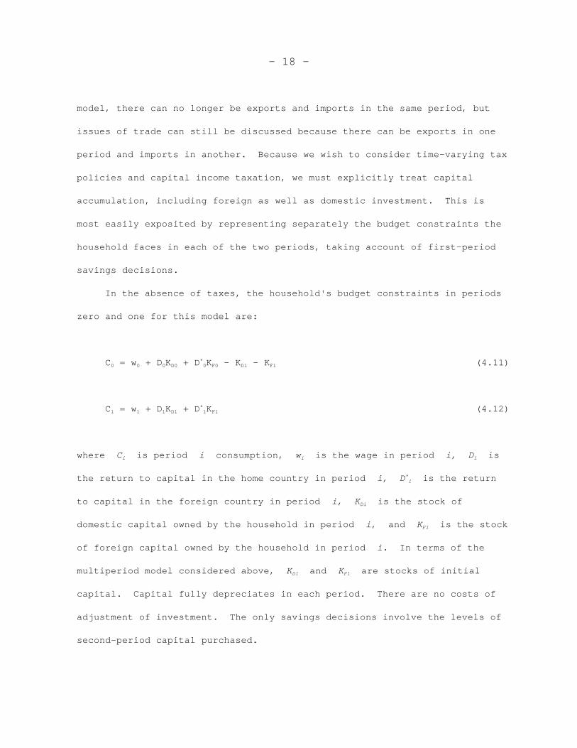
In the absence of taxes, the household's budget constraints in periods

zero and one for this model are:

C = w + D K + D K - K - K (4.11)0 0 0 D0 0 F0 D1 F1*

C = w + D K + D K (4.12)1 1 1 D1 1 F1*

where C is period i consumption, w is the wage in period i, D isi i i

the return to capital in the home country in period i, D is the return*i

to capital in the foreign country in period i, K is the stock ofDi

domestic capital owned by the household in period i, and K is the stockFi

of foreign capital owned by the household in period i. In terms of the

multiperiod model considered above, K and K are stocks of initialD1 F1

capital. Capital fully depreciates in each period. There are no costs of

adjustment of investment. The only savings decisions involve the levels of

second-period capital purchased.

- 19 -

Now let us introduce taxes to this model. In addition to the

consumption taxes and labor income taxes, discussed above, we consider

several taxes on capital income. We make three important distinctions with

respect to these capital income taxes: whether they are assessed at home or

abroad, on the firm or the household, and whether they apply to capital

investment or capital income. These three binary distinctions give rise to

eight types of capital-income tax. Although such a number of tax

instruments may seem excessive, each of these taxes has different economic

effects and all have significant real-world representations. Indeed, there

are still important restrictions implicit in this characterization.

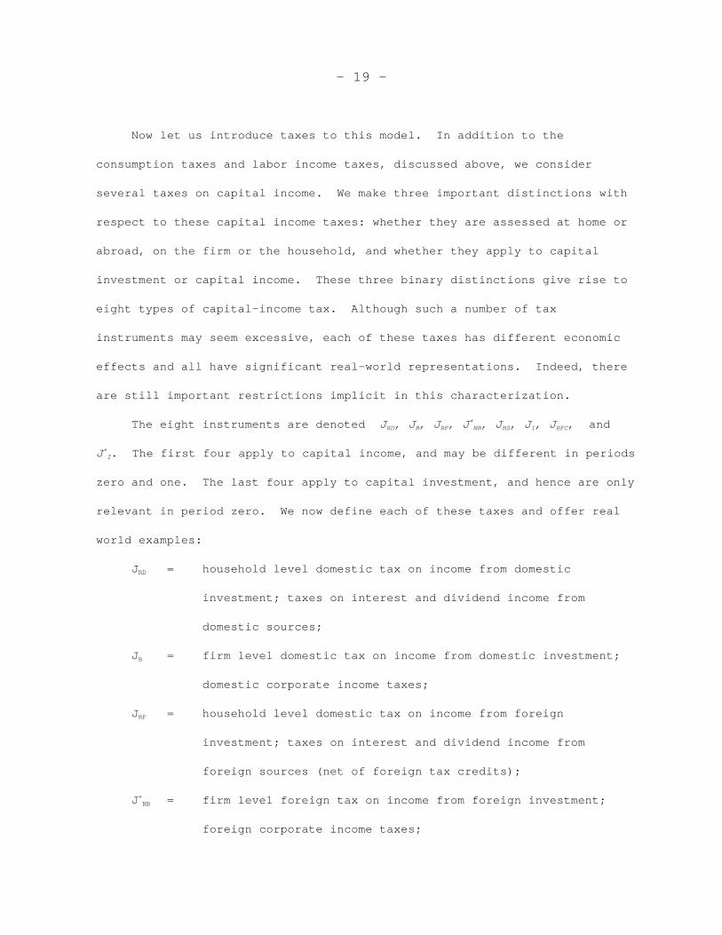
The eight instruments are denoted J , J , J , J , J , J , J , and RD B RF NB HS I RFC*

J . The first four apply to capital income, and may be different in periods*I

zero and one. The last four apply to capital investment, and hence are only

relevant in period zero. We now define each of these taxes and offer real

world examples:

J = household level domestic tax on income from domesticRD

investment; taxes on interest and dividend income from

domestic sources;

J = firm level domestic tax on income from domestic investment;B

domestic corporate income taxes;

J = household level domestic tax on income from foreignRF

investment; taxes on interest and dividend income from

foreign sources (net of foreign tax credits);

J = firm level foreign tax on income from foreign investment;*NB

foreign corporate income taxes;

- 20 -

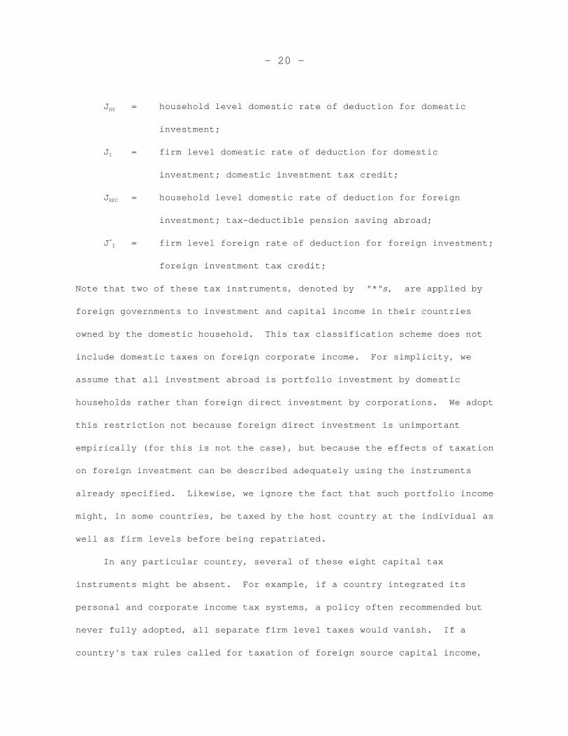
J = household level domestic rate of deduction for domesticHS

investment;

J = firm level domestic rate of deduction for domesticI

investment; domestic investment tax credit;

J = household level domestic rate of deduction for foreignRFC

investment; tax-deductible pension saving abroad;

J = firm level foreign rate of deduction for foreign investment;*I

foreign investment tax credit;

Note that two of these tax instruments, denoted by "*"s, are applied by

foreign governments to investment and capital income in their countries

owned by the domestic household. This tax classification scheme does not

include domestic taxes on foreign corporate income. For simplicity, we

assume that all investment abroad is portfolio investment by domestic

households rather than foreign direct investment by corporations. We adopt

this restriction not because foreign direct investment is unimportant

empirically (for this is not the case), but because the effects of taxation

on foreign investment can be described adequately using the instruments

already specified. Likewise, we ignore the fact that such portfolio income

might, in some countries, be taxed by the host country at the individual as

well as firm levels before being repatriated.

In any particular country, several of these eight capital tax

instruments might be absent. For example, if a country integrated its

personal and corporate income tax systems, a policy often recommended but

never fully adopted, all separate firm level taxes would vanish. If a

country's tax rules called for taxation of foreign source capital income,

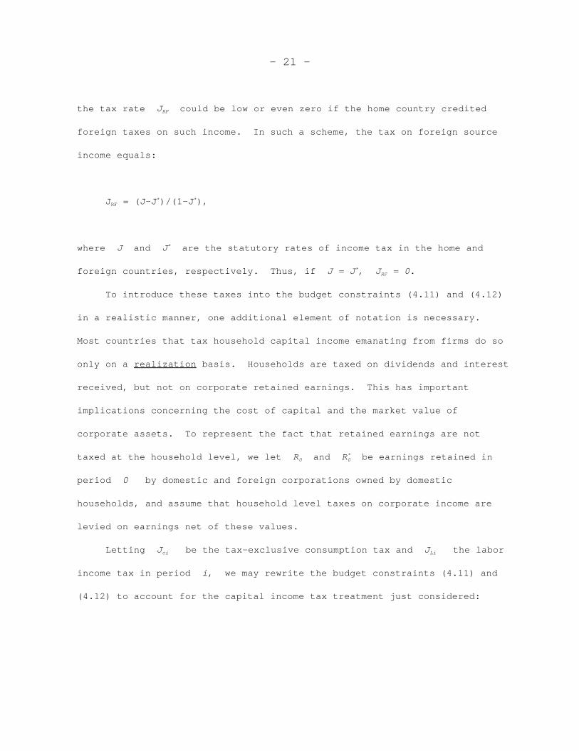
- 21 -

the tax rate J could be low or even zero if the home country creditedRF

foreign taxes on such income. In such a scheme, the tax on foreign source

income equals:

J = (J-J )/(1-J ),RF* *

where J and J are the statutory rates of income tax in the home and*

foreign countries, respectively. Thus, if J = J , J = 0.*RF

To introduce these taxes into the budget constraints (4.11) and (4.12)

in a realistic manner, one additional element of notation is necessary.

Most countries that tax household capital income emanating from firms do so

only on a realization basis. Households are taxed on dividends and interest

received, but not on corporate retained earnings. This has important

implications concerning the cost of capital and the market value of

corporate assets. To represent the fact that retained earnings are not

taxed at the household level, we let R and R be earnings retained in0 0*

period 0 by domestic and foreign corporations owned by domestic

households, and assume that household level taxes on corporate income are

levied on earnings net of these values.

Letting J be the tax-exclusive consumption tax and J the laborci Li

income tax in period i, we may rewrite the budget constraints (4.11) and

(4.12) to account for the capital income tax treatment just considered:

- 22 -

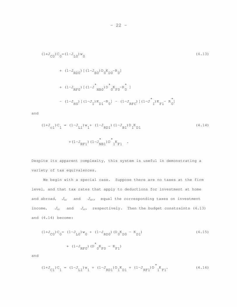
(1+J )C =(1-J )w (4.13) C0 0 L0 0 + (1-J )[(1-J )D K -R ] RD0 B0 0 D0 0 * * * + (1-J )[(1-J )D K -R ] RF0 NB0 0 F0 0 * * - (1-J )[(1-J )K -R ] - (1-J )[(1-J )K - R ] HS I D1 0 RFC I F1 0 and (1+J )C = (1-J )w + (1-J )(1-J )D K (4.14) c1 1 L1 1 RD1 B1 1 D1 * * +(1-J )(1-J )D K . RF1 NB1 1 F1

Despite its apparent complexity, this system is useful in demonstrating a

variety of tax equivalences.

We begin with a special case. Suppose there are no taxes at the firm

level, and that tax rates that apply to deductions for investment at home

and abroad, J and J , equal the corresponding taxes on investmentHS RFC

income, J and J , respectively. Then the budget constraints (4.13)RD RF

and (4.14) become:

(1+J )C = (1-J )w + (1-J )(D K - K ) (4.15) C0 0 L0 0 RD0 0 D0 D1 * + (1-J )(D K - K ) RF0 0 F0 F1 and * (1+J )C = (1-J )w + (1-J )D K + (1-J )D K . (4.16) C1 1 L1 1 RD1 1 D1 RF1 1 F1

- 23 -

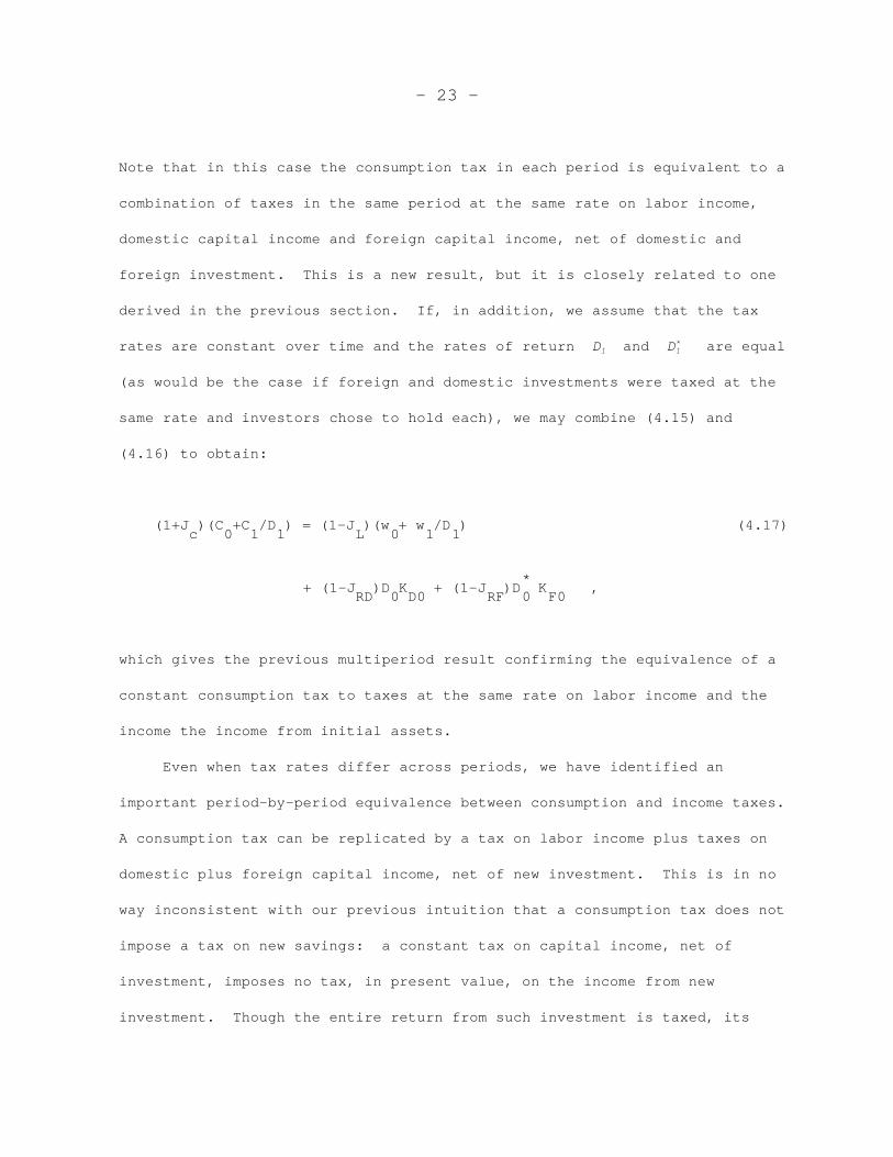
Note that in this case the consumption tax in each period is equivalent to a

combination of taxes in the same period at the same rate on labor income,

domestic capital income and foreign capital income, net of domestic and

foreign investment. This is a new result, but it is closely related to one

derived in the previous section. If, in addition, we assume that the tax

rates are constant over time and the rates of return D and D are equal1 1*

(as would be the case if foreign and domestic investments were taxed at the

same rate and investors chose to hold each), we may combine (4.15) and

(4.16) to obtain:

(1+J )(C +C /D ) = (1-J )(w + w /D ) (4.17) c 0 1 1 L 0 1 1 * + (1-J )D K + (1-J )D K , RD 0 D0 RF 0 F0

which gives the previous multiperiod result confirming the equivalence of a

constant consumption tax to taxes at the same rate on labor income and the

income the income from initial assets.

Even when tax rates differ across periods, we have identified an

important period-by-period equivalence between consumption and income taxes.

A consumption tax can be replicated by a tax on labor income plus taxes on

domestic plus foreign capital income, net of new investment. This is in no

way inconsistent with our previous intuition that a consumption tax does not

impose a tax on new savings: a constant tax on capital income, net of

investment, imposes no tax, in present value, on the income from new

investment. Though the entire return from such investment is taxed, its

- 24 -

entire cost is deducted at the same rate. Thus, the government is simply a

fair partner in the enterprise (though because of its passive role in the

actual operation of the firm, sometimes called a "sleeping" partner). Only

income from capital already in place at the beginning of period 1 is subject

to a true tax, and this tax was seen above to be part of the income-tax-

equivalent scheme.

These foreign and domestic taxes on capital income less investment are

sometimes called cash flow taxes, since they are based on net flows from the

firm. In the case of the foreign tax, the cash-flow tax is a tax on net

capital inflows. In this sense, it is equivalent to a policy of taxing

foreign borrowing and interest receipts and subsidizing foreign lending and

payments of interest. In the domestic literature on taxation, much has been

made of the equivalence between labor income taxes plus business cash flow

taxes and consumption taxes. But in an open economy, this equivalence also

requires the taxation of cash flows from abroad. For otherwise, the

destination-based consumption tax will include an extra piece that is absent

from the tax on labor and domestic capital income net of domestic

investment.

We turn next to issues related to the level of capital income taxation,

business versus household. In the real world, some payments by firms to

suppliers of capital are taxed only at the investor level, without being

subject to a business-level tax. These are interest payments, which are

treated as tax-deductible business expenses. Other payments, dividends, are

typically either partially deductible or not deductible at all. One may

think of the tax rates J and J as representing weighted average taxB NB*

- 25 -

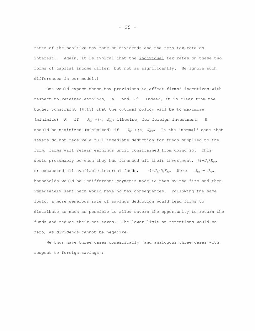
rates of the positive tax rate on dividends and the zero tax rate on

interest. (Again, it is typical that the individual tax rates on these two

forms of capital income differ, but not as significantly. We ignore such

differences in our model.)

One would expect these tax provisions to affect firms' incentives with

respect to retained earnings, R and R . Indeed, it is clear from the*

budget constraint (4.13) that the optimal policy will be to maximize

(minimize) R if J >(<) J : likewise, for foreign investment, R RD HS*

should be maximized (minimized) if J >(<) J . In the "normal" case thatRF RFC

savers do not receive a full immediate deduction for funds supplied to the

firm, firms will retain earnings until constrained from doing so. This

would presumably be when they had financed all their investment, (1-J )K , I D1

or exhausted all available internal funds, (1-J )D K . Were J = J , B 0 D0 RD HS

households would be indifferent: payments made to them by the firm and then

immediately sent back would have no tax consequences. Following the same

logic, a more generous rate of savings deduction would lead firms to

distribute as much as possible to allow savers the opportunity to return the

funds and reduce their net taxes. The lower limit on retentions would be

zero, as dividends cannot be negative.

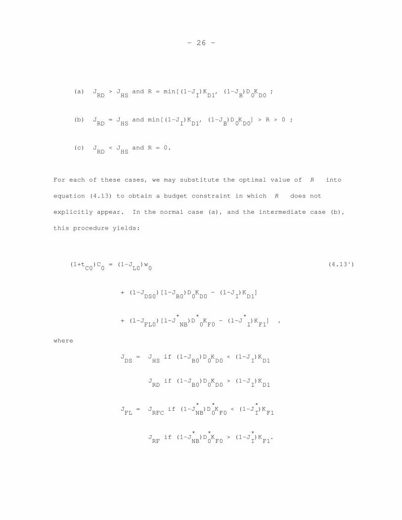
We thus have three cases domestically (and analogous three cases with

respect to foreign savings):

- 26 -

(a) J > J and R = min[(1-J )K , (1-J )D K ; RD HS I D1 B 0 D0 (b) J = J and min[(1-J )K , (1-J )D K ] > R > 0 ; RD HS I D1 B 0 D0 (c) J < J and R = 0. RD HS

For each of these cases, we may substitute the optimal value of R into

equation (4.13) to obtain a budget constraint in which R does not

explicitly appear. In the normal case (a), and the intermediate case (b),

this procedure yields:

(1+t )C = (1-J )w (4.13') C0 0 L0 0 + (1-J )[1-J )D K - (1-J )K ] DS0 B0 0 D0 I D1 * * * + (1-J )[1-J )D K - (1-J )K ] , FL0 NB 0 F0 I F1 where J = J if (1-J )D K < (1-J )K DS HS B0 0 D0 I D1 J if (1-J )D K > (1-J )K RD B0 0 D0 I D1 * * * J = J if (1-J )D K < (1-J )K FL RFC NB 0 F0 I F1 * * * J if (1-J )D K > (1-J )K . RF NB 0 F0 I F1

- 27 -

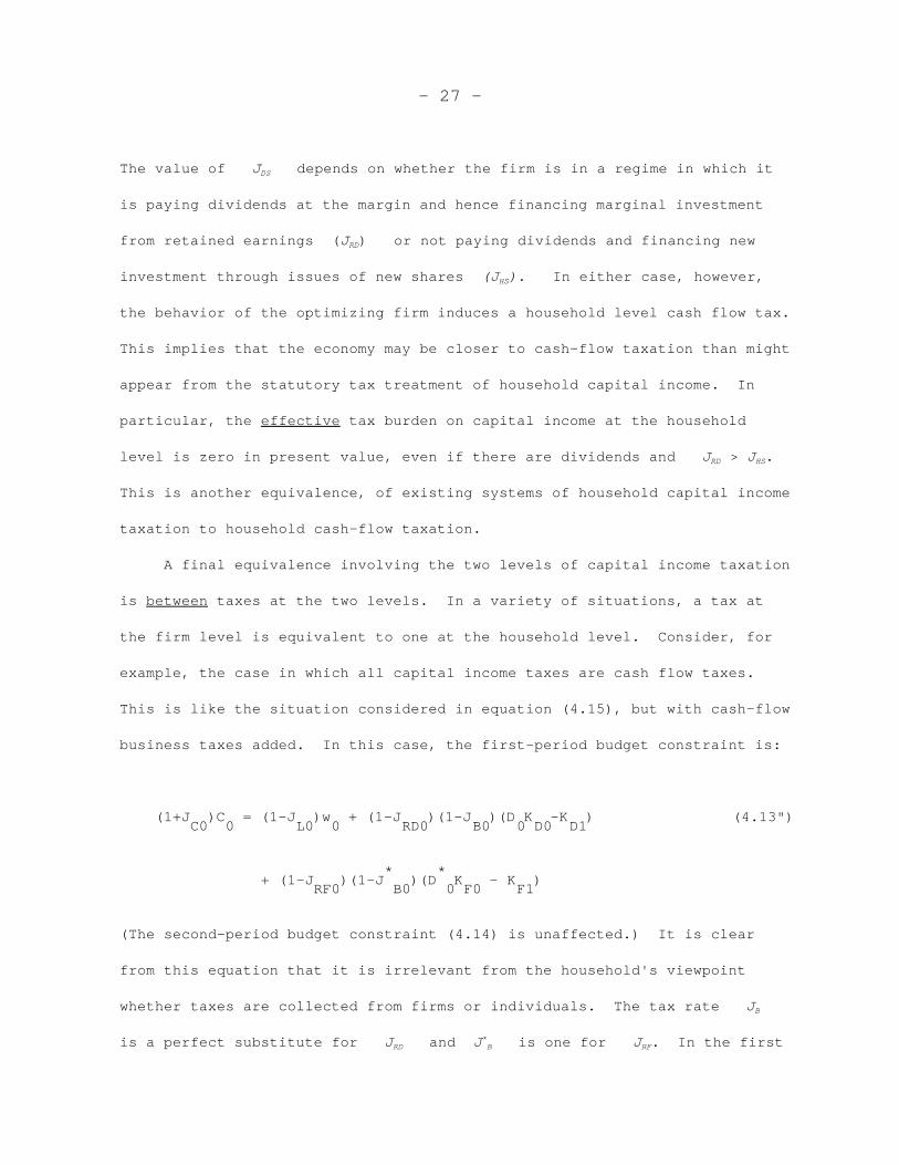
The value of J depends on whether the firm is in a regime in which itDS

is paying dividends at the margin and hence financing marginal investment

from retained earnings (J ) or not paying dividends and financing newRD

investment through issues of new shares (J ). In either case, however,HS

the behavior of the optimizing firm induces a household level cash flow tax.

This implies that the economy may be closer to cash-flow taxation than might

appear from the statutory tax treatment of household capital income. In

particular, the effective tax burden on capital income at the household

level is zero in present value, even if there are dividends and J > J . RD HS

This is another equivalence, of existing systems of household capital income

taxation to household cash-flow taxation.

A final equivalence involving the two levels of capital income taxation

is between taxes at the two levels. In a variety of situations, a tax at

the firm level is equivalent to one at the household level. Consider, for

example, the case in which all capital income taxes are cash flow taxes.

This is like the situation considered in equation (4.15), but with cash-flow

business taxes added. In this case, the first-period budget constraint is:

(1+J )C = (1-J )w + (1-J )(1-J )(D K -K ) (4.13") C0 0 L0 0 RD0 B0 0 D0 D1 * * + (1-J )(1-J )(D K - K ) RF0 B0 0 F0 F1

(The second-period budget constraint (4.14) is unaffected.) It is clear

from this equation that it is irrelevant from the household's viewpoint

whether taxes are collected from firms or individuals. The tax rate J B

is a perfect substitute for J and J is one for J . In the firstRD B RF*

- 28 -

case, with both taxes collected by the same government, the equivalence is

complete; government is indifferent as well. In the second case, this would

not be so, unless a tax treaty existed that directed capital income taxes

collected on specific assets to specific countries regardless of who

actually collect the taxes.

Even in the domestic case, the taxes might appear to have different

effects due to their different collection points. For example, measured

rates of return from the corporate sector would be net of tax were the taxes

collected from firms, but gross of tax were they collected from households.

4.5. Present Value Equivalences

In discussing cash flow taxation, we have made a point that has a more

general application: that tax policies may change the timing of tax

collections without changing their burden, in present value. A constant-

rate cash flow tax exerts no net tax on the returns to marginal investment,

giving investors an initial deduction equal in present value to the ultimate

tax on positive cash flows the investment generates.

In our two-period model, a cash-flow tax at a constant rate collects

revenue equal in present value only to the cash flows from the first-period

capital stock. Thus, an initial wealth tax on that stock would be

equivalent from the viewpoint of both household and government. For

example, consider the simple case with no firm-level taxes and constant tax

rates examined above. This is the example in which the first-period and

second-period budget constraints can be combined as in the multiperiod model

of the previous section. These three budget constraints (first-period,

- 29 -

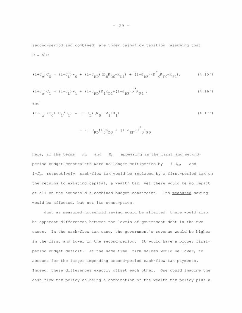
second-period and combined) are under cash-flow taxation (assuming that

D = D ):*

* (1+J )C = (1-J )w + (1-J )(D K -K ) + (1-J )(D K -K ), (4.15') c 0 L 0 RD 0 D0 D1 RF 0 F0 F1 * (1+J )C = (1-J )w + (1-J )D K +(1-J )D K , (4.16') c 1 L 1 RD 1 D1 RF F1 and (1+J )(C + C /D ) = (1-J )(w + w /D ) (4.17') c 0 1 1 L 0 1 1 * + (1-J )D K + (1-J )D K RD 0 D0 RF 0 F0

Here, if the terms K and K appearing in the first and second-D1 F1

period budget constraints were no longer multiperiod by 1-J , and RD

1-J , respectively, cash-flow tax would be replaced by a first-period tax onRF

the returns to existing capital, a wealth tax, yet there would be no impact

at all on the household's combined budget constraint. Its measured saving

would be affected, but not its consumption.

Just as measured household saving would be affected, there would also

be apparent differences between the levels of government debt in the two

cases. In the cash-flow tax case, the government's revenue would be higher

in the first and lower in the second period. It would have a bigger first-

period budget deficit. At the same time, firm values would be lower, to

account for the larger impending second-period cash-flow tax payments.

Indeed, these differences exactly offset each other. One could imagine the

cash-flow tax policy as being a combination of the wealth tax policy plus a

- 30 -

decision by the government to borrow in the first-period and force firms to

accept loans of equal value at the market interest rate, to be repaid in the

same period. Firms would require less funds from the household sector,

leaving households just enough extra money to purchase the bonds floated by

the government.

Thus, the explicitly measured government debt is not an accurate

indicator of policy, since it may vary considerably between the two

equivalent situations. One may think of the "forced loans" of the cash-flow

tax system as being off-budget assets that cause the deficit to be

overstated, assets that can be brought on budget by recalling the loans,

paying back the debt, and shifting to the wealth tax.

One can imagine many similar examples of present value equivalences,

none of which go beyond the bounds of the realistic tax policies we have

already considered. The government can arbitrarily change the measured

composition of a household's wealth between government debt and tangible

capital (and indeed between government debt and human capital, through

changes in the time pattern of labor income taxation) simply by introducing

offsetting levels of debt and "forced loans" attached to these other assets.

This is true whether or not the asset owners are domestic residents or not.

Foreign owners of a domestic corporation that is suddenly hit with a cash-

flow tax on new investment (i.e., excluding the wealth tax effect on

preexisting capital) will spend less of their funds on the domestic firms

and the remainder on other assets, quit possibly the government debt, but

not in the country's external debt, i.e., the aggregate value of domestic

assets owned by foreigners.

- 31 -

It is noteworthy that the government's ability to shift such asset

values of foreigners is more circumscribed than its ability with respect to

domestic residents. It cannot, for example, cause a reduction in the value

of a foreigner's human capital offset by a loan to the foreigner (by cutting

labor income taxes today and raising them in the future) because it cannot

tax the foreigner's labor income. All adjustments with respect to external

debt must be through the tax treatment of foreign-owned domestic assets.