Intragenerational Mobility of the Top Earners in Israel ...

Intragenerational Mobility of the Top Earners in Israel before and

after the Global Financial Crisis

Stav Federman∗, Assaf Sarid†, and Meir Yaish‡

This Version: December 10, 2019

Abstract

The rise in income inequality and the Global Financial Crisis have shifted the attention to analyzing

the top income earners and their mobility. In this paper we contribute to this strand of the

literature in different ways. First, we use different statistical tests to estimate different measures of

intragenerational mobility. This is an improvement to the methodologies used in existing literature,

which usually used descriptive statistics to describe mobility. Second, we use the Global Financial

Crisis as a case study to analyze how major macroeconomic events affect intragenerational mobility

among the top income earners. Using a panel data on the income levels of 22,601 individuals for the

period between 1999-2013, we find that the intragenerational mobility of the top income earners

has declined during the analyzed period. We also find that the Global Financial Crisis had a minor

and transitory effect, if any, on the intragenerational mobility of the top income earners in Israel.

1 Introduction

Income inequality has risen in many advanced economies in the past several decades (OECD, 2011).

Due to this ongoing rise in inequality, accompanied by the Global Financial Crisis of 2008, different

protest movements such as Occupy Wall Street have shifted their attention to social and economic

mobility of the top income earners, and in particular, the top 1%. While this segment of the popula-

tion is important in understanding inequality and mobility dynamics, it has attracted little research

attention.∗Department of Economics, University of Haifa†Department of Economics, University of Haifa‡Department of Sociology, University of Haifa

1

In this study we attempt to measure the intragenerational mobility of the top income earners in

Israel for the period 1999-2013. We use longitudinal income data of 22,601 individuals, who were born

in Israel between 1963 and 1973.1 Such a long period is quite unique in the intragenerational mobility

literature of the top income earners, where the period analyzed ranges between six years (Jenderny,

2016) and ten (Auten and Gee, 2009), with one exception of nineteen years (Saez and Veall, 2005).

Hence, we are among the first ones that can look at intragenerational mobility in permanent income

and how it is affected by transitory shocks to income in a more thorough analysis than previous studies

did.

The data include both employment and labor incomes. After normalizing all incomes to 2014

shekels as a base year, we measure the intragenerational mobility using all known methodologies.

Most of these methodologies usually rely on descriptive statistics. To deepen our understanding, we

employ two statistical methodologies that were not used in this strand of the literature previously.

These allow us to test statistically our results and to better document intragenerational mobility in

Israel during this period.

The fact that we look at a specific cohort in its beginning of the economic life cycle enables us

to overcome some of the methodological problems in measuring intragenerational mobility, as all the

individuals in the sample are in a period in which their income does not decline (as opposed to older

individuals). Hence, our measures are more accurate, as they are driven merely by economic factors,

and not life cycle characteristics.

We use three different measures of intragenerational mobility. First, we estimate the persistence

rate. This measure attempts to estimate the probability that an individual who belonged to a specific

fractile at a certain year, belongs to it also after a given number of years. Previous studies, which

used this measure, calculated it by looking at the proportion of individuals who belonged to a specific

fractile in two different points in time. We take the methodology of calculating the persistence rate

one step forward by employing a linear probability model with binary variables which indicate if an

individual belonged to a specific fractile in different years. Not only does this methodology allows

us to estimate accurately the persistence rate, but it also enables us to test statistically the degree

of mobility in the economy during this period. Using the methodology, we show that the annual

persistence rate in Israel between 1999 and 2013 equaled on average 66.4% for the top 1%, 77.8% for

1We exclude immigrants from the sample, which allows us to focus on labor market factors which affect mobility.For a thorough discussion of the issue, see section 3.

2

the top 5% and 81.1% for the top 10%. On an international comparison, the persistence rates we found

set Israel below the persistence rate found in the U.S. (Auten et al., 2013) and Germany (Jenderny,

2016), with similar levels to Finland (Jantti et al., 2010). This is quite surprising, because the Israeli

labor market is more similar to the one in the United States than to the one in Finland.

The next measure we use is the Individual Rank Standard Deviation, which was first introduced

by Jenderny (2016): For each individual in the sample we assign his rank among all income earners

in each year, and compute his rank standard deviation over time. The underlying idea behind this

measure is that a higher rank standard deviation implies a higher mobility, because it means that the

rank movements individuals experience are larger. Using this measure, we find that the top 1% was

less mobile than the 5%, which in turn was less mobile than the top 10%.

Finally, we use a measure, which analyzes changes in the share of income held by the top fractiles

over periods of different lengths. The idea springs from Shorrocks (1978b), and it relies on the assump-

tion, that if mobility is high, the share of the top income fractiles tends to decline in the permanent

income (relative to their annual income). This is because when mobility is high, the changes in annual

income are high as well, and therefore the permanent income declines. Based on this notion, we mea-

sure the Top Income Mobility measure, and show that the top fractiles experienced a downward trend

in mobility in the analyzed period and that the members of the top 1% experienced bigger variations

in incomes relative to the top 5% and 10%.

Previous studies presented the Top Income Mobility measure as a measure of mobility which is

based on changes of the income distribution. This measure, however, is descriptive, and consequently,

one cannot derive from it any statistical inference. To deepen our understanding if indeed the average

annual income distribution and the permanent income are different, we use the Kolmogorov-Smirnov

test. This test is used to examine if two distributions are different, and if the pdf of one is always

higher than the other. In our case, the annual income distribution of the top income earners should

always be higher than the permanent income of the top income earners. We test this hypothesis for

every 5 years sub-period and find that the permanent income distribution is significantly lower than

the annual income distribution in more than 70% of the sub-periods.

Last but not least, we use all these measures to examine if major economic events have affected

the intragenerational mobility of the top fractiles. While social mobility researchers have long been

interested in the impact of macroeconomic forces on intragenerational mobility, we know little about

3

the impact of macroeconomic shocks on intragenerational mobility in general and on the upper fractiles

in particular (See, for example, Yu (2010)). During the period we analyze, Israel, as many other

countries on the globe, suffered from the Global Financial Crisis of 2008. It was a macroeconomic

event that a-priori should have affected intragenerational mobility, as 28% of the top 1% were employed

in the high-tech sector and the financial sector in the time of the crisis (Ben-Naim and Belinsky, 2012).

Indeed, as can be seen in Figure 8, the wages of the top income earners (as well as in other fractiles)

declined during these two events.

Under these circumstances, one would expect that such events should increase intragenerational

mobility, because they suffered the most from these events. Nevertheless, the results depict a different

picture: while the persistence rate during 2008 indeed declined, this decline was transitory, and a

year later the persistence rate rose again and continued in its upward trend. Similar results are

obtained using the Kolmogorov-Smirnov test, as it shows that the permanent income distribution was

significantly smaller than the annual income distribution for the top 1% during the Global Financial

Crisis. We conclude from these results that such shocks, despite their major impact on wages and

employment, affected intragenerational mobility in a very minor manner.

2 Literature Review

The research regarding top income earners is mainly focused on their income shares, based on annual

tax records. Such studies were conducted in many countries, including France (Atkinson and Piketty,

2007), Germany (Dell, 2007), Canada (Saez and Veall, 2005), The United Kingdom (Atkinson, 2007),

The Netherlands (Salverda and Atkinson, 2007) and The U.S (Atkinson and Piketty, 2007). The

evolution of the shares of the top income earners in the vast majority of the countries was strikingly

similar: a substantial fall in the first half of the 20th century, followed by a rise since the 1980s. The

U.S has experienced the most significant increase in top earners’ income shares, while the income

concentration increase was less severe in European countries.

Studies concerning the intergenerational mobility of the top fractiles are less common since panel

data of those fractiles’ members are hard to obtain. For this reason, the available research on the

mobility of the top fractiles is mainly concerned with intragenerational mobility. There are two main

mobility measurements used in the literature. The first is the persistence rate: the probability of an

individual who belonged to a top fractile in a specific year to stay in the same fractile after a certain

4

period of time. Studies using this method were conducted in Canada (Saez and Veall, 2005), France

(Landais, 2008), the U.S (Auten et al., 2013; Auten and Gee, 2009), Norway (Aaberge et al., 2013)

and Germany (Jenderny, 2016). We add to this literature in two ways: First, we employ the linear

probability model to estimate the persistence rate, and thus we provide a statistical tool to test the

evolution of the persistence rate over time. Second, we use data on Israeli income earners for a long

period of time, thus contribute to the understanding of intragenerational mobility of the top fractiles

in another advanced economy.

The second mobility measure is based on Shorrocks (1978a,b) who showed that mobility has an

equalizing effect on income concentration when it is calculated for a longer period. Specifically, if a

society is very mobile, and the incomes of those at the top and at the bottom of the income distribution

change from one year to the next, then the average income of members of those groups will converge in

the long run. Hence, by comparing the annual income shares of the top fractiles to the corresponding

average shares over a longer period one can estimate mobility. This method was used to measure

mobility in Canada (Saez and Veall, 2005), Norway (Aaberge et al., 2013) and Germany (Jenderny,

2016). Again, we extend the common methodology used and use the Kolgomorov-Smirnov test in

order to analyze distributional changes over time.

A third mobility measure, proposed by Jenderny (2016), is the Individual Rank Standard De-

viation (IRSD). This measure is based on the changes each individual experiences in her rank (the

relative position among all income earners). We use all three measures, and attempt to deepen our

understanding of the top income earners’ mobility by using methods that allow to determine whether

these measures are statistically significant.

While the research regarding top income shares and mobility is becoming more and more common,

in Israel it remains scarce. Most of the research regarding mobility in Israel concerns mobility across

the income distribution (Aloni and Krill, 2017; Frish and Zussman, 2009; Beenstock, 2002; Romanov

and Zussman, 2003). The only study analyzing the mobility of the top income earners was conducted

by Ben-Naim and Belinsky (2012), who calculated the persistence rate of the top 10, 1 and 0.1 percent

between the years 1999-2009. They found that the one year persistence rate was 86% for the top 10

percent, 70% for the top 1 percent and 50% for the top 0.1 percentiles. Ben-Naim and Belinsky also

found that 33.4% of those who belonged to the top 1 percent in 1999 were also a part of that fractile

in 2009. We differ from their paper by using two measures that were never used on Israeli data: the

5

Distribution Analysis and the Individual Rank standard Deviation. Moreover, we use data for a longer

period. These additional procedures further deepen understanding of the mobility of the top fractiles

in Israel.

3 Data

To answer our research question, we construct a panel of individuals born in Israel between 1963

and 1973. The first dataset we use consists of 25,085 individuals who were sampled in the 1995

census, constructed by the Israel Central Bureau of Statistics. The sample constitutes 4% of all Israeli

population, and it includes each individual’s demographic characteristics such as gender, ethnicity,

religion and marital status.2,3

The census dataset is merged to another dataset from The Israeli Tax Authority, which reports

the annual gross business and employment incomes of each individual in the sample for the years

1999 to 2013. The employment incomes are based on registered annual gross earnings as reported

by the employer. The business incomes are based on registered annual gross earnings that originated

from self-employment. Both the employment and business earnings in the dataset are before personal

income taxes and all deductions. In addition, all incomes were adjusted to 2014 New Israeli Shekel. We

followed a standard practice in analyzing such data and excluded from the sample individuals, whose

average earning from both business and labor was lower than 1000 New Israeli Shekels a year. These

individuals might have had another source of income not included in our dataset, hence considering

them as a low income earners may bias our results. After excluding the very low income earners, our

sample contains 22,601 individuals for which we have data on their income for the entire period.

We analyze mobility for two main concepts of income: employment income and total income, which

is defined as the sum of employment and business incomes. To assure that the existence of individuals

with zero incomes does not bias our results, we also use as a robustness check a sub-sample, which

consists only of individuals who reported positive incomes in the entire period we analyze. This sub-

sample contains 10,533 individuals. The summary statistics of the different income concepts in the

different samples is presented in Table 1. For each of these types of income, we calculate the permanent

income, which is defined as the arithmetic mean of annual incomes over a specific time period. In

2These characteristics were collected in the 1995 census, and as such are not longitudinal.3In the population we focus on, the top fractiles, there is very little variation in the demographic characteristics, and

therefore the analysis based on these characteristics is omitted.

6

particular, we calculate the permanent income for periods of three, five and fifteen years. Finally, for

each individual, we assign the fractile to which he belongs, based on his position relative to all other

individuals in the sample. We do so both for annual and permanent income. The permanent income

for the entire sample and the top fractiles are presented in Table 2.

Table 1: Summary Statistics

Observations MeanStandardDeviation

Minimum Maximum

Entire sample

Permanent total in-come

25,085 99,243 112,974 0 4,340,400

Permanent employ-ment income

25,085 84,119 96,920 0 3,623,900

Sample excluding permanent total incomes smaller than 1,000


22,601 110,140 113,871 1,000 4,340,400


22,601 93,183 97,947 0 3,623,900

Sample containing positive incomes only


10,533 153,828 120,064 8,550 1,990,100


8,665 142,257 104,652 7,550 1,245,800

Note: The permanent income corresponds to the mean income over 15 years.

In most of the analyses, scholars have studied individuals from different stages in their life cycle.

This might bias the estimation of intragenerational mobility, as individuals in different stages of

the life cycle may experience different income dynamics. Young individuals tend to experience an

upward trend in their income as they accumulate human capital through learning-by-doing, whereas

older individuals may experience different trends. These different trends may be the consequence of

Table 2: Permanent incomes

3 years 5 years 15 years Observations

Entire sample 110,639 110,470 110,140 22,601

top 10% 365,340 367,686 360,695 2,260

top 5% 459,347 462,789 452,630 1,130

Top 1% 720,046 726,116 710,262 226

Note: The permanent income over x years is calculated as the average of all x years permanentincomes.

7

either sorting into different career paths, or due to tasks that deteriorate health and performed by

only a segment of the population. Indeed, empirical studies, which followed the life-cycle earnings,

found supporting evidence for these different trends (Heckman et al., 2003; Lagakos et al., 2018).

Moreover, this effect can be observed in the Israeli data as well. Figure 1 presents the mean and

standard deviation of employment income by age in Israel in the year 2005. It can be seen that

the mean employment income increases with age for ages 25-35, and decreases for ages 60-65. Older

ages are also characterized by larger standard deviation, meaning that incomes are more dispersed

for older individuals. Consequently, such a trend might bias mobility measures upwards. Fortunately,

this problem does not exist in our analysis: the red line in Figure 1 indicates the age of the oldest

individual of our sample, suggesting that our sample contains individuals who are at the stage of the

life-cycle previous to the income decrease.

Figure 1: Mean employment income by age, 2005

Source: Own computation, based on data from the 2005 household expenditure survey conducted byIsrael Central Bureau of Statistics

As mentioned above, our sample consists only on individuals born in Israel, and thus excludes all

immigrants who migrated to Israel during the 1990s post-soviet immigration wave. Immigrants usually

8

experience low income levels in the first years in their new country and relatively a high mobility in

the following years, as they acquire the necessary human and social capital (Cardoso, 2006). These

two effects might bias downwards mobility measures. Thus, focusing only on Israeli-born individuals

helps us in overcoming this potential bias.4

4 Methodology

In this section we present the three main mobility indicators we use in the paper: the Persistence Rate,

the Individual Rank Standard Deviation and the Distribution Analysis. Each measure shed light on

a different angle of mobility and overcomes hurdles from other measures, as is explained bellow.

4.1 The Persistence Rate

We first measure mobility by the probability of individuals, who belonged to the top fractile in a

specific year to stay in the same fractile in the consecutive year(s). This measure is common in the

literautre (e.g. (Jenderny, 2016), (Jantti et al., 2010) and (Auten et al., 2013)). A common descriptive

procedure to compute the persistence rate between t and t+ τ is to divide the number of individuals

who belonged to the analyzed fractile in both t and t+ τ by the number of individuals who belonged

to this fractile in time t. Such a procedure might be vulnerable for statistical inference, as one cannot

test if the persistence rate is statistically significant. To overcome this problem, we estimate the

persistence rate with a simple linear probability model.5

In particular, consider the following model:

Pert+τi = α+ β · Perti + εi, (1)

where Perti is a dummy variable that equals 1 if individual i belonged to fractile φ at time t and zero

otherwise, and εi is a random noise. Note that such a model is based on two dummies, and as such

its coefficients have an economic significance, which allows us to calculate the persistence rate.

Our population has two groups. The first one consists of all individuals who did not belong to

fractile φ at year t. For this group Perti = 0. The other group, who were in fractile φ at year t, are the

4This problem may affect more severely some of the indices we use, such as the Individual Rank Standard Deviation,explained in Section 4.2.

5As will be explained below, our variables are binary, and hence our linear probability model is identical to ANOVA.

9

ones for which Perti = 1. The intercept, α, equals the mean of Pert+τi among those who were not in

fractile φ in time t. Hence, the intercept provides us the upward mobility to fractile φ between years

t and t+ τ .

Next, note that the persistence rate is the probability that an individual who belonged to fractile

φ in year t, also belonged to the same fractile in year t+ τ . This is the mean of the second group (i.e.,

those whose Perti = 1). In our model, this mean is α+β. Hence, our linear probability model provides

us a useful tool to measure both the upward mobility into the top fractiles and the persistence rate,

as well as to test their statistical significance. We test that both α and β are statistically different

from zero. Furthermore, we wish to show that α+β 6= 1, which implies no intragenerational mobility.

To do so, we use the statistical rule that var(α+ β) = var(α) + var(β) + 2cov(α, β). We compute the

variance of both α and β, and use the idea that cov(α, β) < 0. This last idea stems from the fact that

α represents the upward mobility (and thus the downward mobility), and β is an increasing function

of the persistence rate (as we show in Appendix A). Thus, a higher persistence rate implies a higher β

and by the same time a lower α. As a result, we compute var(α) and var(β) and use var(α) + var(β)

as an upper bound for var(α + β). Following Jenderny (2016), Jantti et al. (2010) and Auten et al.

(2013), we set τ to 1, 3 and 5 years.

The persistence rate discussed above is unconditional of survival in the years between t and t+ τ .

We also derive the conditional persistence rate: the probability of an individuals who belonged to the

top fractile in year t to stay in the same fractile in all of the years between t+ 1 and t+ τ . We do so

by estimating the same linear probability model described in equation (1), where Pert+τi equals one if

the individual belonged to fractile φ in all years between t+1 and t+τ , and 0 otherwise. As explained

above, α+ β equals the mean value in Pert+τi of the individuals who belonged to fractile φ in t, which

in this case equals the conditional persistence rate.

4.2 Individual Rank Standard Deviation

Another measure we use to analyze the intragenerational mobility is the Individual Rank Standard

Deviation (IRSD), proposed by Jenderny (2016). This measure is based on the standard deviation of

each individual’s rank (the relative position among all income earners). The individual rank standard

10

deviation is computed as follows:

IRSDi =

√∑15t=1(ri,t − ri)2

14(2)

where ri,t is the rank of individual i in year t, and ri is individual i’s average rank. A higher mobility

implies more changes in the rank, and as a result a higher IRSD.

Note that this measure is based on the entire population in the sample, and as a result, it allows

us to compare groups of different sizes from the sample. Second, note that this measure is individual

specific; As a result, we can analyze the distribution of the IRSD. Specifically, for the top 1, 5 and

10 percent of income earners,6 we compare the mean and the median of the IRSD, among other

distributional characteristics of this distribution.

4.3 Distribution Analysis

This mobility measure is based on Shorrocks (1978a,b), who showed that in a more mobile economy,

the concentration of top income earners tends to decline as the analyzed period is longer. The intuition

behind this result is that in a mobile economy individuals may belong to different fractiles in different

years, and thus the permanent income distribution is more concentrated than the annual income

distribution. Thus, the higher the mobility, the higher the difference between these two distributions.

Following Aaberge and Mogstad (2013), we measure the mobility of the top 1, 5, and 10 fractiles

of income earners by the change in the annual income shares of those fractiles and their permanent

income shares. In particular, for each sub-period of three and five years between the years 1999 and

2013, we calculate the permanent income of each individual. Based on the permanent incomes, we

calculate the permanent income share of the 1, 5, and 10 top income fractiles. Then we calculate the

annual income share of those fractiles. Finally, we calculate the Top Income Mobility (TIM) curve,

defined as the difference between the two income shares. Let Zt denote the annual income share of

the fractile at stake, and let Zτ,T denote the permanent income share between the years τ and T of

6The top income earners in this case are defined as the top permanent income earners of the entire period.

11

the same fractile. Then, the TIM is given by:7

TIMt =1

T

T∑t=τ

Zt − Zτ,T . (3)

Note that a higher TIM implies more mobility, because if individuals move between income groups,

average annual top income concentration ( 1T

∑Tt=τ Zt) is higher than the concentration of the average

income (Zτ,T ). Note that the TIM does not allow us to compare groups of different sizes, because it

is an absolute and not a relative measure. In order to compare the mobility of the top fractiles to one

another and to the results found in other studies, we also compute the TIM in relative terms:

TIM relt =

1T

∑Tt=τ Zt − Zτ,T1T

∑Tt=τ Zt

. (4)

While the TIM provides us a useful tool for measuring mobility, it is descriptive, and does not

allow to determine the statistical significance of our results. To overcome this problem, we use the two-

sample Kolmogorov-Smirnov test, which checks whether two distributions differ and whether one of

them contains smaller values than the other. This test enables us to verify that the permanent income

distribution among the top fractiles is indeed more concentrated than the annual income distribution

of the top fractiles, thus include smaller values, and whether this difference is statistically significant.

We calculate the Kolmogorov-Smirnov to compare the permanent income of the top 1%, 5% and 10%

between the years t and t+ 4 and the annual income of the same fractiles in t+ 2.

5 Results

5.1 Persistence Rate

Figures 2, 3 and 4 present the persistence rate after one, three and five years for the top 1, 5 and

10 percent of total income earners. As explained in section 4.1, the persistence rate is derived by

the linear probability model described in equation 1, and calculated as α + β. The lower and upper

bounds in these figures corresponds to the confidence interval, calculated by var(α) + var(β). As can

be seen in the figures, α+β is significantly lower than 1 (that is, no mobility) and higher than 0 (that

7The permanent income is calculated as the average income for both three and five years. Thus, for each year, wecalculate total permanent income as the sum of the permanent income of all individuals, and the total income of thetop fractile as the sum of permanent income of all the individuals who belong to this fractile, based on their permanentincome. Zτ,T is defined as the fraction between the two.

12

is, almost full mobility), for all of the fractiles and for one, three and five years.

As evident in figures 3 and 4, both the top 5 and top 10 percents experienced an increasing trend

in their persistence rate after one, three and five years. The persistence rate of the top 5% was 72%

after one year, 53.2% after three years and 53.4% after five years in 1999, and rose by the end of the

period to 79.8%, 66.2% and 59%, respectively. The persistence rate of the top 10% in 1999 was 74.8%

after one year, 63.3% after three years and 59.8% after five years, and they rose by the end of the

period to 83.1%, 73.5% and 66.4%, respectively. Note that the lower bound of the persistence rate

of the top 5% and 10% in the latest two years is higher than the upper bound in the first two years,

suggesting that this upward trend is significant. The persistence rate after one and five years of the

top 1% shows an increasing trend as well. The persistence rate after one year rose from 62.8% to

66.3%, and the persistence rate after five years rose from 36.7% to 43.3%. However, its persistence

rate after three years does not show an upward trend. Except for a fall in 2000 and a rise in 2009, the

persistence rate after three years of the top 1% is relatively stable, at around 50%.

Another interesting point is that the persistence rate kept rising even during and after the global

financial crisis. The only exception is the persistence rate after one year of the top 1%, which fell in

2008. A possible explanation might be found in the fact that 15% of the individuals in the top 1% were

employed in the financial sector in the years 2003-2009 (Ben-Naim and Belinsky, 2012), suggesting

that the top 1% is more sensitive to financial events. Nonetheless, the effect of the financial crisis was

only temporary: the persistence rate after one year of the 1% recovers quickly. We elaborate on this

point in section 6.

To ensure that the results are not biased by choice of income concept, the persistence rate was also

calculated for employment income, and for sample that contains only positive incomes. The results

can be found in Appendix B. The trends of the persistence rate in all income concepts are similar

to the trends in Figures 2, 3 and 4. However, the persistence rate of all fractiles are higher when

calculated for employment income, indicating that the employment incomes are more stable compared

to total incomes.

We now turn to compare our results to the ones obtained in previous studies which estimated the

persistence rate in the U.S, Germany and Finland. Jenderny (2016) found that between the years

2001 and 2006, the persistence rate of the top 1% in Germany was 75% after one year and 65% after

three years, and for the top 5% it was 85% after one year and 75% after three years. Thus, the

13

Figure 2: Persistence rate of the top 1% total income earners


German persistence rate for both fractiles and time lags are higher than the persistence rate of the

corresponding Israeli fractiles. In Finland, on the other hand, the persistence rate after one year of

the top 1% was 64.7% in the years 2001-2002 (Jantti et al., 2010), a similar persistence rate to its

14


counterpart in Israel in the same year.

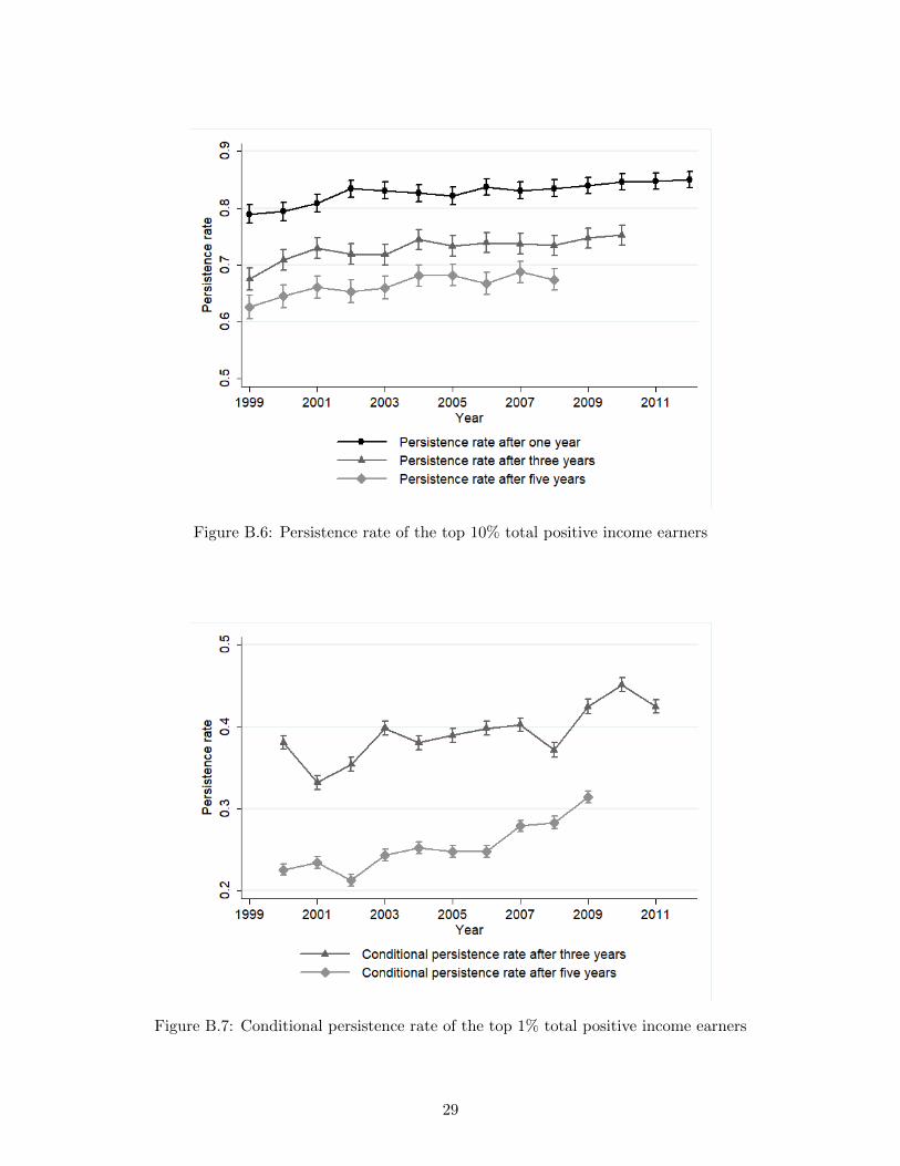
The persistence rate of the 1% between the years 1999-2009 in the U.S. was calculated condition-

ally.8 The conditional persistence rate of the top fractiles in Israel is reported in Appendix Figures

B.7, B.8 and B.9. The conditional persistence rate of the top 1% in the U.S ranged from 52% to 66%

after one year, 29% to 43% after three years and 21% to 32% after five years (Auten et al., 2013).

Our calculations for the Israeli top 1% shows that its persistence rate after one year is higher and the

persistence rate after three years is lower than the corresponding fractile in the U.S. Hence, for longer

time intervals, the top 1% is characterized by a higher mobility.

5.1.1 Comparing Groups of Different Size

A potential bias to the persistence rate might arise from the group size: A smaller group size might

bias mobility upwards because the same decline in absolute rank might generate a higher probability to

leave a smaller group. This potential bias makes it difficult to compare the mobility of the top fractiles

with each other. A naıve solution could be to split the larger group to sub-groups of similar size and

compare their persistence rate.9 However, since in the top fractiles upward mobility is impossible by

8For a detailed explanation between the unconditional and conditional persistence rates see section 4.1.9For example, to split the top 5 percent of income earners to five groups, each consists of one percentile.

15

definition, we calculate the probability of not moving downwards for the top and next-to-top fractiles

of the same size. This allows us to compare the same type of mobility to equally sized groups. To do

so, we use the same regression model described by equation 1, where the left-hand side of the equation

equals 1 if the individual belonged to fractile φ or above in t+ τ and 0 otherwise. In this case, α+ β

will equal the probability of not moving down. The results are reported in Table 3.

In all of the years examined and for both lags of three and five years, the 5% was more likely to

not move downwards than the lower income groups of the same size. Moreover, the lower bound of

the confidence interval of the top 5% was higher than the upper bound of the other groups, except

for 2002. This indicates that the probability of not moving downwards of the top 5% is significantly

higher than that of the lower fraciles. These results suggest that the top 5% is in fact less mobile than

the top 10%, since when taking group-size into account, the top 5% are less mobile than the rest of

the members of the top 10%.

The results for the top 1% are less clear. Although the probability of not moving down of the top

1% was higher than the probability of lower income fractiles in the years in 1999 and 2003, it was

lower in the rest of the years. Moreover, examining the confidence intervals shows the probability in

1999 and 2003 of the top 1% was not significantly higher. This means we can not determine whether

the top 1% was more or less mobile than lower income groups.

5.2 Individual Rank Standard Deviation

Figure 5 shows the distribution of the Individual Rank Standard Deviation of the top fractiles. The

table shows the corresponding values. The boxes show the 25th, 50th and 75th percentiles of the

IRSD, and the whiskers show the 5th and 95th percentiles. The white circles show the mean IRSD,

and the black lozenges show the fractile size. The top fractiles are defined by average income over 15

years. The figure displays clearly that the top 1 percent had a lower IRSD compared to the top 5 and

10 percent: The mean IRSD of the top 1 percent is lower than the mean IRSD of the top 5 and 10

percent, as well as the P95, P75, P50, P25 and P05. The IRSD of the top 5 percent was also lower

than the IRSD of the top 10 percent, but to a lesser degree. Hence, the members of higher fractiles

were less prone to rank changes.

The IRSD also demonstrates the effect of the group size on the persistence rate, which was discussed

in section 5.1.1. As can be seen in Figure 5, more than 95% of the members of the top 1 percent are

16

Table 3: Upward mobility of fractiles of the same size, calculated for total income

% of fractile members who did not move downwards

Three years Five years

1999-2004 1999-2002

Fractile Fractile Fractile Fractile

71-7543.98

9538.5

71-7537.96

9527.88

(40.63, 47.32) (35.1, 41.87) (34.6, 41.31) (24.45, 31.27)

76-8046.55

9636.28

76-8039.12

9633.19

(43.39, 49.69) (33.17, 39.38) (35.94, 42.27) (30.06, 36.29)

81-8543.32

9740.71

81-8537.14

9735.84

(40.42, 46.22) (37.93, 43.48) (34.21, 40.03) (33.04, 38.62)

86-9044.73

9835.4

86-9042.96

9841.15

(42.16, 47.29) (32.9, 37.81) (40.37, 45.52) (38.74, 43.54)

91-9548.85

9936.28

91-9549.29

9941.15

(46.75, 50.94) (34.33, 38.24) (47.18, 51.38) (39.21, 43.08)

96-10053.45

10036.73

96-10058.23

10051.33

(52.07, 54.82) (35.38, 38.06) (56.9, 59.55) (50.09, 52.56)

2002-2007 2003-2006

71-7555.22

9538.5

71-7555.66

9540.27

(51.89, 58.53) (35.1, 41.87) (52.33, 58.98) (36.87, 43.65)

76-8053.72

9634.96

76-8057.88

9638.05

(50.57, 56.83) (31.83, 38.06) (54.74, 60.98) (34.94, 41.14)

81-8553.19

9738.05

81-8557.26

9737.61

(50.3, 56.05) (35.26, 40.82) (54.39, 60.11) (34.82, 40.39)

86-9052.39

9834.51

86-9056.64

9841.15

(49.84, 54.92) (32.09, 36.92) (54.11, 59.14) (38.74, 43.54)

91-9553.01

9938.05

91-9558.58

9944.25

(50.92, 55.07) (36.1, 40) (56.54, 60.61) (42.31, 46.16)

96-10054.42

10036.28

96-10064.69

10046.89

(53.06, 55.78) (34.94, 37.62) (63.44, 65.93) (45.63, 48.17)

2005-2010 2007-2010

71-7542.83

9537.17

71-7556.99

9543.36

(39.48, 46.17) (33.76, 40.55) (53.66, 60.3) (39.98, 46.74)

76-8046.28

9640.27

76-8059.73

9647.35

(43.13, 49.43) (37.16, 43.35) (56.61, 62.85) (44.26, 50.42)

81-8549.38

9738.5

81-8563.19

9748.23

(46.48, 52.26) (35.7, 41.27) (60.34, 66.02) (45.47, 50.98)

86-9051.59

9842.48

86-9064.07

9848.23

(49.04, 54.12) (40.08, 44.86) (61.58, 66.55) (45.85, 50.59)

91-9551.95

9937.61

91-9560.8

9952.65

(49.86, 54.02) (35.65, 39.55) (58.76, 62.81) (50.76, 54.52)

96-10059.03

10041.59

96-10065.22

10047.79

(57.71, 60.33) (40.28, 42.9) (63.98, 66.45) (46.52, 49.05)

Note: Brackets correspond to the confidence interval, calculated by var(α) + var(β).

17

characterized by an IRSD larger than 287.95. Since the group size of the top 1% is 226, more than

95% of the top 1% experienced rank change that was big enough for them to exit the fractile. As

mentioned before, the top 1% had a lower IRSD compared to the top 5% and 10%. This suggests

that despite the fact that the rank movement of the top 1% was smaller than the rank movement of

the top 5% and 10%, a bigger proportion of the top 1% left the fractile due to group size. Thus, the

group size biased persistence rate downwards. 10

Top 10 Top 5 Top 1

P95 7317.13 7416.76 6494.44

P75 4551.38 4209.39 1566.79

P50 1672.59 1067.85 522.52

P25 665.83 495.7 325.42

P05 327.95 300.65 287.95

Mean of IRSD 2697.54 2301.26 1528.03

Fractile’s size 2,260 1130 226

Figure 5: Individual Standard Deviation of Annual Ranks, calculated for labor and business incomes

Notes: Boxes correspond to P25, P50, and P75 percentile points of individual standard deviationsof annual ranks (IRSD). Whiskers correspond to P5 and P95 percentile points. Fractiles defined byaverage income over 15 years.

To ensure that the results are not biased by the choice of income variable and the existence of

individuals with income of zero, we calculate the IRSD for a sample of employment income only, and

for a sample of only positive incomes. The results are reported in Appendix Figures C.1, C.2 and C.3.

In all of the samples, we get a similar result: the IRSD of the top 1 percent is smaller than the IRSD

of the top 5 and 10 percent. Indicating that mobility decreases as income increases.11

10To overcome the effect of group size on the persistence rate, we also compare groups of similar size in section 5.1.111When calculated for labor income, the top one percent’s P95 of IRSD is larger than the corresponding figure of the

top 5 and 10 percent. However, the top 1 percent is still characterized by the smallest mean IRSD.

18

5.3 Distribution Analysis

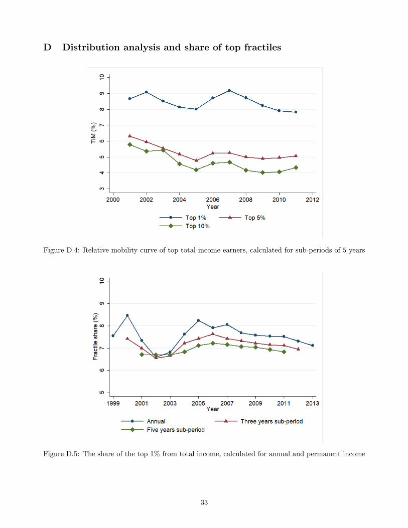
Figure 6 presents the TIM of the top 1%, 5% and 10%, calculated for sub-periods of 5 years. The

annual and permanent income shares on which the TIM is based on are presented in Appendix Figures

D.5, D.6 and D.7. It is evident from the figure that the TIM of the top 5% and 10% was decreasing

during the period: from 2.02 and 1.4 in 2001, to 1.6 and 1.1 in 2011, respectively. The TIM of these

two fractiles increase in 2006 and 2007, followed by a decrease. This increase is driven by a transitory

rise in annual income shares in 2005, which increase the left hand side of the TIM, as described in

equation 3.

This downward trend in the TIM indicates that the mobility of the top 5% and 10% is decreasing.

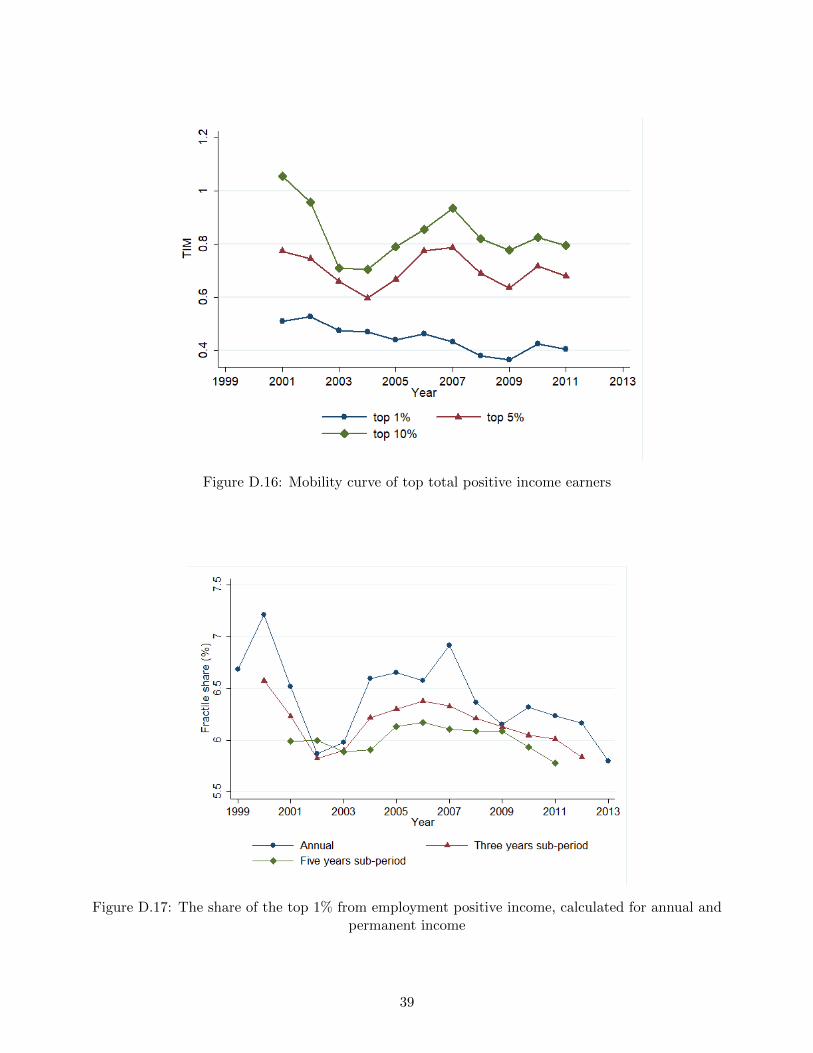
However, The mobility of the top 1% was relatively stable: between the years 2001 and 2011, the

TIM of the 1% ranged from 0.58 to 0.68, with minor up and down movements. The TIM was also

calculated for employment income, and for sample that contains only positive incomes. The results

can be found in Appendix D. For all income concepts, there is a downward trend in TIM, indicating

our results were not biased by choice of income concept.

For all of the top fractiles, the Kolmogorov-smirnov test results show that the permanent income

distribution is significantly more concentrated than the annual income distribution for more than 70%

of the sub-periods.12 Surprisingly, the financial crisis of 2008 seems to have no effect on the mobility

of the top fractiles, as well as on their income shares. We elaborate this point in section 6.

To compare mobility among the top fractiles, we turn to the relative TIM, which is presented in

Appendix Figure D.4. It is clear from the figure that the top 1% had the higher TIM in relative terms,

indicating that the members of the top 1% were more mobile in terms of income changes. Moreover,

the top 5% was more mobile than the top 10%. suggesting that mobility increases as income increases.

We now turn to compare our results to those found in studies conducted in other countries. The

absolute and relative TIM were also computed in Germany (Jenderny, 2016) and Norway (Aaberge

et al., 2013) for sub-periods of 3 years, in the years 2001-04. For both the absolute and relative TIM,

the mobility of the top 1%, 5% and 10% in Israel was higher than the mobility of the corresponding

fractiles in Germany. As for the comparison to Norway, while the top 10% in Israel is more mobile

than its Norwegian counterpart throughout the period, the mobility of the top 1% and 5% in Israel is

higher in the first two sub-periods, but lower in the end of the period. 13

12The results of the Kolmogorov-Smirnov test are presented in Appendix Tables E.2, E.3 and E.4.13The full comparison can be found in Appendix Table D.1.

19

Figure 6: Mobility curve of top total income earners, calculated for sub-periods of 5 years

6 Macroeconomic Shocks and Intragenerational Mobility

Up to this point we estimated the intragenerational mobility in three different methodologies, yet the

period we analyse allows us to use the Great Financial Crisis as a test case to examine how macroeco-

nomic shocks affect intragenerational mobility among the top income earners. While social mobility

researchers have long been interested in the impact of macroeconomic forces on intragenerational

mobility, we know little about the impact of macroeconomic shocks on intragenerational mobility in

general and on the upper fractiles in particular.

A large portion of the top fractiles in Israel were employed either in the high-tech sector or in the

financial sector. Hence, we can exploit the Global Financial Crisis of 2008 as a major macroeconomic

shock, which a-priori should have hit the upper fractiles. Indeed, as Figure 7 and 8 show, the average

incomes of the top fractiles declined dramatically during the crisis.

There are several reasons to think why the Global Financial Crisis should have affected the in-

tragenerational mobility of the top income earners. As discussed above, a large portion of the top

income earners worked either in the financial sector or in the high-tech sectors. The Crisis could have

affected wages in these sectors either directly, due to losses the firms in these sectors encountered, or

indirectly, as funds for investment in the high-tech sector were lower during the financial crisis.

20

Figure 7: Average employment incomes by deciles

Source: Own computation, based on data from the household expenditure surveys conducted byIsrael Central Bureau of Statistics

We analyze the impact of the Global Financial Crisis on intragenerational mobility looking at two

of the measures we presented above: the persistence rate and the distributional analysis. Using the

persistence rate, we show that the effect of the Global Financial Crisis on the top fractiles intragener-

ational mobility was minor. In particular, as Figure 2 shows, during the crisis the top 1% experienced

a sharp decline in its persistence rate (from 65.9% to 62.3%), yet it recovered during the following

year. Furthermore, the persistence rate of the top 5% and top 10%, as shown in Figures 3 and 4, was

not affected by the Global Financial Crisis.

Looking at the distributional analysis, we get to the same conclusions. As Figure 6 shows, the

mobility curve continues its downward trend also during and after the Crisis, suggesting that despite

transitory changes in income levels, the relative position of the upper fractiles persisted to be higher

and increase over time. We conclude from these two measures that the Global Financial Crisis had a

minor impact, if any, on the intragenerational mobility among the top fractiles in Israel.

Furthermore, using the Kolmogorov-Smirnov test we find that for the top 1% the permanent income

distribution had significantly smaller values than the annual income distribution, for all sub-period

except 2002-2006 and 2003-2007. In particular, the test shows no special effect of the Global Financial

21

Figure 8: Average employment incomes of the top 5 percentiles

Source: Own computation, based on data from the household expenditure surveys conducted byIsrael Central Bureau of Statistics

Crisis on the mobility of the top 1%, as the difference between the annual income distribution and

permanent income distribution is statistically significant and greater than 0. For the top 5% and 10%,

the test shows similar results for the sub-periods prior to 2007, but it is not significant for the sub-

period of 2008-2012. The test’s results are significant again in 2009-2013 for both groups, indicating

that if the Global Financial Crisis had only a transitory effect on mobility. 14

7 Conclusions

The Global Financial Crisis and the rising income inequality have shifted the attention to intragenera-

tional mobility among the top fractiles. We contribute to this strand of the literature in several ways:

First, we employ new methodologies to measure intragenerational mobility among the top income

earners. These methodologies help us in better estimating the persistence rate and the distributional

changes between annual income and permanent incomes. Second, we focus on a specific cohort, whose

members are all in the same stage in the life cycle. This helps us estimate only the part of the mobility

14The results of the Kolmogorov-Smirnov test are presented in Appendix Tables E.2, E.3 and E.4.

22

which is the result of market forces, rather than selection to different career paths or other distortions

that occur over the life cycle. Finally, we exploit the Global Financial Crisis to analyze how a major

macroeconomic event affect intragenerational mobility among the top income earners.

several arguments may prove understanding intragenerational mobility among the top fractiles

important. First, there is no reason to believe that the mobility patterns of different income groups

are similar (Bjorklund et al., 2012), therefore, shading light on a specific income group can deepen

our understanding of the mobility in a society. Second, mobility of the top income earners off-sets

some of the problems rising from income concentration, such as the political power of those who have

economical power and the fact that the benefits of growth are enjoyed by a smaller group. When the

top income earners are mobile, economic and political power shifts between individuals, and a bigger

portion of the population benefits from growth (Jenderny, 2016).

Using a panel of incomes of 22,601 individuals for the period between 1999-2013, we present

several results: First, using different measures of mobility, we show that the top income earners have

experienced a decline in their mobility in the analysed period. This result is robust to different income

concepts and different sub-periods we analyze. Second, we show that the Global Financial Crisis of

2008 had a very minor effect, if any, on intragenerational mobility in Israel, despite the fact that a

large portion of the top fractiles were employed in the financial and high-tech sectors.

References

Aaberge, R., Atkinson, A. B. and Modalsli, J. (2013). The ins and outs of top income mobility,

Discussion Papers 762, Technical report, Statistics Norway, Research Department.

Aaberge, R. and Mogstad, M. (2013). Income mobility as an equalizer of permanent income, Technical

Report 769, Statistics Norway Research department, Discussion Papers 769.

URL: http://ideas.repec.org/p/ssb/dispap/769.html

Aloni, T. and Krill, Z. (2017). Intergenerational income mobility in israel— international and sectoral

comparisons, Technical report, Ministry of Economics, Office of Chief Economist, Jerusalem.

Atkinson, A. B. (2007). The distribution of top incomes in the united kingdom 1908–2000, Top In-

comes over the Twentieth Century: A Contrast between Continental European and English-Speaking

Countries 1: 82–140.

23

Atkinson, A. B. and Piketty, T. (2007). Top incomes over the twentieth century : a contrast between

continental European and English-speaking countries, Oxford University Press.

Auten, G. and Gee, G. (2009). Income Mobility in the United States: New Evidence from Income Tax

Data.

URL: https://www.jstor.org/stable/41790506

Auten, G., Gee, G. and Turner, N. (2013). Income inequality, mobility, and turnover at the top in the

US, 1987-2010, American Economic Review 103(3).

Beenstock, M. (2002). Intergenerational mobility: Earnings and education in Israel, Technical report,

Maurice Falk Institute for Economic Research in Israel.

URL: http://primage.tau.ac.il/libraries/brender/booksf/1931093.pdf

Ben-Naim, G. and Belinsky, A. (2012). Wage divergence in israel: Analysis of wage mobility over the

last decade, Israel Ministry of Finance - Economics and Research Department .

Bjorklund, A., Roine, J. and Waldenstrom, D. (2012). Intergenerational top income mobility in

Sweden: Capitalist dynasties in the land of equal opportunity?, Journal of Public Economics 96(5-

6): 474–484.

URL: https://www.sciencedirect.com/science/article/abs/pii/S0047272712000163

Cardoso, A. R. (2006). Wage mobility: Do institutions make a difference?, Labour Economics

13(3): 387–404.

Dell, F. (2007). Top incomes in Germany throughout the twentieth century: 1891–1998, in A. B.

Atkinson and T. Piketty (eds), Top Incomes over the Twentieth Century: A Contrast Between Con-

tinental European and English Speaking Countries, Oxford University Press, New York, chapter 9,

pp. 365–425.

Frish, R. and Zussman, N. (2009). The Effect of Parents’ Education and Childhood Environment on

their Children’s Education, Technical report.

URL: http://citeseerx.ist.psu.edu/viewdoc/download?doi=10.1.1.595.8761&rep=rep1&type=pdf

Heckman, J. J., Lochner, L. J. and Todd, P. E. (2003). Fifty years of mincer earnings regressions,

Technical report, National Bureau of Economic Research.

24

Jantti, M., Riihela, M., Sullstrom, R. and Tuomala, M. (2010). Trends in Top Income Shares in

Finland, in A. B. Atkinson and T. Piketty (eds), Top incomes: a global perspective, Oxford University

Press, New York, chapter 8, pp. 371–448.

Jenderny, K. (2016). Mobility of Top Incomes in Germany, Review of Income and Wealth 62(2): 245–

265.

Lagakos, D., Moll, B., Porzio, T., Qian, N. and Schoellman, T. (2018). Life cycle wage growth across

countries, Journal of Political Economy 126(2): 797–849.

Landais, C. (2008). Top Incomes in France: booming inequalities?, Technical report, Paris School of

Economics, Mimeo.

OECD (2011). An overview of growing income inequalities in oecd countries: main findings, Divided

We Stand: Why Inequality Keeps Rising .

Romanov, D. and Zussman, N. (2003). Labor Income Mobility and Employment Mobility in Israel,

1993-96, Israel Economic Review 1(1): 81–102.

URL: https://papers.ssrn.com/sol3/papers.cfm?abstract id=2171743

Saez, E. and Veall, M. R. (2005). The Evolution of High Incomes in Northern America: Lessons from

Canadian Evidence, American Economic Review 95(3): 831–849.

Salverda, W. and Atkinson, A. B. (2007). Top incomes in the netherlands over the twentieth century,

Top Incomes over the Twentieth Century: A Contrast between Continental European and English-

Speaking Countries pp. 426–71.

Shorrocks, A. (1978a). Income inequality and income mobility, Journal of Economic Theory 19: 376–

393.

Shorrocks, A. F. (1978b). The Measurement of Mobility, Technical Report 5.

Yu, W.-h. (2010). Enduring an economic crisis: The effect of macroeconomic shocks on intragenera-

tional mobility in japan, Social science research 39(6): 1088–1107.

25

Appendix

A Deriving β

Let λ denote the persistence rate and φ the analyzed fractile (φ = 0.01 when analyzing the top 1%,

for example). Then,

β =cov(Pert+τi ,Perti)

var(Perti)2

=

∑i

(Pert+τi − Per

t+τ)(

Perti − Pert)

∑i

(Perti − Per

t)2 =

λ− φ1− φ

, (5)

where the last equality stems from the definition of the persistence rate, λ and a fractile. Note that

with no mobility (that is, a persistence rate of 1), the estimated coefficient equals 1, whereas with full

mobility (that is, a persistence rate of 0), the estimated coefficient is negative. Hence, an estimated

coefficient of 0 implies a high rate of mobility, in which λ = φ. Clearly, one can derive λ from β for

any chosen φ.

B Persistence rate for different concepts of income

Figure B.1: Persistence rate of the top 1% employment income earners

26



27

Figure B.4: Persistence rate of the top 1% total positive income earners


28


Figure B.7: Conditional persistence rate of the top 1% total positive income earners

29



30

C IRSD for different concepts of income

Top 10 Top 5 Top 1

P95 7464.835 7628.19 8441.64

P75 4639.3 4315.32 2314.71

P50 1814.6 1147.34 543.73

P25 640.15 505.14 428.32

P05 3 375.48 351.45 348.58

Mean of IRSD 2840.82 2576.58 1830.9

Fractile’s size 2,260 1,130 226

Figure C.1: Individual Standard Deviation of Annual Ranks, calculated for labor income

Top 10 Top 5 Top 1

P95 2699.91 2506.73 1159.69

P75 1164.59 812.56 343.51

P50 502.53 364.80 106.87

P25 247.12 161.75 46.43

P05 85.12 46.43 23.51

Mean of IRSD 858.758 671.233 312.1538

Fractile’s size 1,053 526 105

Figure C.2: Individual Standard Deviation of Annual Ranks, calculated for positive labor andbusiness incomes

31

Top 10 Top 5 Top 1

P95 2204.69 2059.54 1472.18

P75 805.55 606.09 262.43

P50 349.13 255.24 73.46

P25 174.05 119.42 35.68

P05 64.52 35.68 18.31

Mean of IRSD 643.07 520.22 281.42

Fractile’s size 866 433 86

Figure C.3: Individual Standard Deviation of Annual Ranks, calculated for positive labor income

32

D Distribution analysis and share of top fractiles

Figure D.4: Relative mobility curve of top total income earners, calculated for sub-periods of 5 years

Figure D.5: The share of the top 1% from total income, calculated for annual and permanent income

33



34

Figure D.8: The share of the top 1% from employment income, calculated for annual and permanentincome

Figure D.9: The share of the top 5% from employment income, calculated for annual and permanentincome

35

Figure D.10: The share of the top 10% from employment income, calculated for annual andpermanent income

Figure D.11: Mobility curve of top employment income earners

36

Figure D.12: Relative mobility curve of top employment income earners

Figure D.13: The share of the top 1% from total positive income, calculated for annual andpermanent income

37



38

Figure D.16: Mobility curve of top total positive income earners

Figure D.17: The share of the top 1% from employment positive income, calculated for annual andpermanent income

39



40

Figure D.20: Mobility curve of top employment positive income earners

Table D.1: Comparison of top income earners’ mobility in Israel, Norway and Germany

Israel

Absolute TIM Relative TIM (%)

Year 2001 2002 2003 2004 2001 2002 2003 2004Top 10% 1.26 1.34 1.10 0.98 3.58 3.86 3.15 2.72Top 5% 0.92 0.87 0.76 0.70 4.11 4.00 3.48 3.05Top 1% 0.47 0.37 0.36 0.34 6.35 5.31 5.11 4.54

Norway


Year 2001 2002 2003 2004 2001 2002 2003 2004Top 10% 0.81 0.8 0.81 0.9 2.5 2.37 2.27 2.54Top 5% 0.73 0.71 0.78 0.91 3.25 2.97 2.96 3.53Top 1% 0.63 0.62 0.78 0.96 6.04 5.23 5.57 7.37

Germany


Year 2001 2002 2003 2004 2001 2002 2003 2004Top 10% 0.43 0.4 0.41 0.4 1.55 1.46 1.45 1.41Top 5% 0.37 0.35 0.34 0.34 1.99 1.88 1.8 1.76Top 1% 0.25 0.23 0.22 0.23 3.18 2.95 2.73 2.66

Source: Germany: Jenderny (2016), Norway: Aaberge et al. (2013)

41

E Kolmogorov-smirnov test

Table E.2: Top 1% Kolmogorov-Smirnov test results for sub-periods of 5 years

1999-2003 2003-2007 2007-2011

Smallergroup

D P-value Smallergroup


D P-value

1:00 0.36 0 1:00 0.1244 0.031 1:00 0.16 0.003

2:00 0 1 2:00 0 1 2:00 -0.0311 0.804

Combined 0.36 0 Combined 0.1244 0.061 Combined 0.16 0.006

2000-2004 2004-2008 2008-2012

Smallergroup



D P-value

1:00 0.2444 0 1:00 0.1822 0.001 1:00 0.1911 0

2:00 -0.0356 0.752 2:00 0 1 2:00 0 1


2001-2005 2005-2009 2009-2013

Smallergroup



D P-value

1:00 0.0133 0.961 1:00 0.2756 0 1:00 0.2222 0

2:00 -0.2889 0 2:00 0 1 2:00 -0.0089 0.982

Combined 0.2889 0 Combined 0.2756 0 Combined 0.2222 0

2002-2006 2006-2010Smallergroup


D P-value

1:00 0.0844 0.201 1:00 0.3111 02:00 0 1 2:00 0 1

Combined 0.0844 0.399 Combined 0.3111 0

Note: For each sub-period the test compares the permanent income distribution of the top fractile to the annualincome distribution of the top fractile in the middle year. Group 1 is the permanent income distribution, group2 is the annual income distribution.

42


1999-2003 2003-2007 2007-2011

Smallergroup



D P-value

1:00 0.3097 0 1:00 0.0681 0.005 1:00 0.0814 0.001

2:00 0 1 2:00 0 1 2:00 -0.0062 0.958


2000-2004 2004-2008 2008-2012

Smallergroup



D P-value

1:00 0.2257 0 1:00 0.069 0.005 1:00 0.0496 0.062

2:00 -0.0071 0.945 2:00 0 1 2:00 0 1


2001-2005 2005-2009 2009-2013

Smallergroup



D P-value

1:00 0.0027 0.992 1:00 0.1531 0 1:00 0.0876 0

2:00 -0.1027 0 2:00 0 1 2:00 -0.0018 0.996

Combined 0.1027 0 Combined 0.1531 0 Combined 0.0876 0

2002-2006 2006-2010Smallergroup


D P-value

1:00 0.0469 0.083 1:00 0.2027 02:00 -0.0168 0.727 2:00 0 1



43


1999-2003 2003-2007 2007-2011

Smallergroup



D P-value

1:00 0.2527 0 1:00 0.0518 0.002 1:00 0.0407 0.024

2:00 0 1 2:00 0 1 2:00 -0.0031 0.979


2000-2004 2004-2008 2008-2012

Smallergroup



D P-value

1:00 0.2159 0 1:00 0.0615 0 1:00 0.0248 0.25

2:00 -0.0035 0.972 2:00 0 1 2:00 -0.0018 0.993

Combined 0.2159 0 Combined 0.0615 0 Combined 0.0248 0.492

2001-2005 2005-2009 2009-2013

Smallergroup



D P-value

1:00 0.0013 0.996 1:00 0.1319 0 1:00 0.0708 0

2:00 -0.0518 0.002 2:00 0 1 2:00 -0.0009 0.998

Combined 0.0518 0.005 Combined 0.1319 0 Combined 0.0708 0

2002-2006 2006-2010Smallergroup


D P-value

1:00 0.0487 0.005 1:00 0.1841 02:00 0.0084 0.852 2:00 0 1



44

Date post:	05-Apr-2022
Category:	Documents
Upload:	others
View:	3 times
Download:	0 times

Intragenerational Mobility of the Top Earners in Israel ...

Documents