1IntroductIon to AnAlog And MIxed-SIgnAl electronIcS
1.1 IntroductIon
“In the beginning, there were only analog electronics and vacuum tubes and huge, heavy, hot equipment that did hardly anything. Then came the digital—enabled by integrated circuits and the rapid progress in computers and software—and electronics became smaller, lighter, cheaper, faster, and just better all around, all because it was digital.” That’s the gist of a sort of urban legend that has grown up about the nature of analog electronics and mixed-signal electronics, which means simply electronics that has both analog and digital circuitry in it.
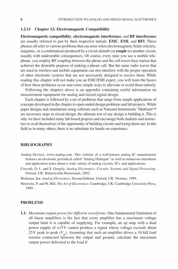
Like most legends, this one has some truth to it. Most electronic systems, ever since the time that there was anything around to apply the word “electronics” to, were analog in nature for most of the twentieth century. In electronics, an analog signal is a voltage or current whose value is proportional to (an analog of) some physical quantity such as sound pressure, light intensity, or even an abstract numerical value in an analog computer. digital signals, by contrast, ideally take on only one of two values or ranges of values and by doing so represent the discrete binary ones and zeros that form the language of digital computers. To give you an idea of how things used to be done with purely analog systems, Figure 1.1 shows on the left a two-channel vacuum-tube audio amplifier that can produce about 70 W per channel.
The vacuum-tube amplifier measures 30 cm × 43 cm × 20 cm and weighs 17.2 kg (38 lb) and was state-of-the-art technology in about 1955. On its right is a solid-state class D amplifier designed in 2008 that can produce about the same amount of
0002254126.indd 1 2/1/2015 4:35:52 PM
COPYRIG
HTED M
ATERIAL
2 InTrODucTIOn TO AnALOg AnD MIxeD-SIgnAL eLecTrOnIcS
output power. It is a mixed-signal (analog and digital) design. It measures only 15 cm × 10 cm × 4 cm and weighs only 0.33 kg, not including the power supply, which is of comparable size and weight. The newer amplifier uses its power devices as switches and is much more efficient than the vacuum-tube unit, which is about 50 times its size and weight. So the claim that many analog designs have been made completely obsolete by newer digital and mixed-signal designs is true, as far as it goes.
Sometimes, you will hear defenders of analog technology argue that “the world is essentially analog, and so analog electronics will never go away completely.” Again, there’s some truth to that, but it depends on your point of view. The physics of quantum mechanics tells us that not only are all material objects made of discrete things called atoms but many forms of energy appear as discrete packets called quanta (photons, in the case of electromagnetic radiation). So you can make just as good an argument for the case that the whole world is essentially digital, not analog, because it can be represented as bits of quanta and atoms that are either there or not there at all.
The fact of the matter is that while the bulk of today’s electronics technology is implemented by means of digital circuits and powerful software, a smaller but essential part of what goes into most electronic devices involves analog circuitry. even if the analog part is as simple as a battery for the power supply, no one has yet developed a battery that behaves digitally: that is, one that provides an absolutely constant voltage until it depletes and drops abruptly to zero. So even designers of an otherwise totally digital system have to deal with the analog problem of power-supply characteristics.
This book is intended for anyone who has an interest in understanding or designing systems involving analog or mixed-signal electronics. That includes undergraduates with a basic sophomore-level understanding of electronics, as well as more advanced undergraduates, graduate students, and professionals in engineering, science, or other fields whose work requires them to learn about or deal with these types of electronic systems. The emphasis is practical rather than theoretical, although enough
FIgure 1.1 A comparison: Vacuum‐tube audio amplifier (left) using a design circa 1955 and class D amplifier (right) using a design circa 2008.
0002254126.indd 2 2/1/2015 4:35:52 PM
OrgAnIZATIOn OF THe BOOK 3
theory to enable an understanding of the essentials will be presented as needed throughout. Many textbooks present electronics concepts in isolation without any indication of how a component or circuit can be used to meet a practical need, and we will try to avoid that error in this book. Practical applications of the various circuits and systems described will appear as examples, as paper or computer-simulation design exercises, and as lab projects.
1.2 orgAnIzAtIon oF the Book
The book is divided into three main sections: devices and linear systems (chapters 2 and 3), linear and nonlinear analog circuits and applications (chapters 4–7), and special topics of analog and mixed-signal design (chapters 8–12). A chapter-by-chapter summary follows.
1.2.1 chapter 2: Basics of electronic components and devices
In this chapter, you will learn enough about the various types of two‐ and three‐terminal electronic devices to use them in simple designs. This includes rectifier, signal, and light‐emitting diodes and the various types of three‐terminal devices: field‐effect transistors (FeTs), bipolar junction transistors (BJTs), and power devices. Despite the bewildering number of different devices available from manufacturers, there are usually only a few specifications that you need to know about each type in order to use them safely and efficiently. In this chapter, we present basic circuit models for each type of device and how to incorporate the essential specifications into the model.
1.2.2 chapter 3: linear System Analysis
This chapter presents the basics of linear systems: how to characterize a “black box” circuit as an element in a more complex system, how to deal with characteristics such as gain and frequency response, and how to define a system’s overall specifications in terms that can be translated into circuit designs. The power of linear analysis is that it can deal with complex systems using fairly simple mathematics. You also learn about some basic principles of noise sources and their effects on electronic systems.
1.2.3 chapter 4: nonlinearities in Analog electronics
While linear analysis covers a great deal of analog‐circuit territory, nonlinear effects can both cause problems in designs and provide solutions to other design problems. noise of various kinds is always present to some degree in any circuit, and in the case of high‐gain and high‐sensitivity systems dealing with low‐level signals, noise can determine the performance limits of the entire system. You will be introduced to the basics of nonlinearities and noise in this chapter and learn ways of dealing with these issues and minimizing problems that may arise from them.
0002254126.indd 3 2/1/2015 4:35:52 PM
4 InTrODucTIOn TO AnALOg AnD MIxeD-SIgnAL eLecTrOnIcS
1.2.4 chapter 5: op Amp circuits in Analog electronics
The workhorse of analog electronics is the operational amplifier (“op amp” for short). Originally developed for use in World War II era analog computers, in integrated‐circuit form the op amp now plays essential roles in most analog elec-tronics systems of any complexity. This chapter describes op amps in a simplified ideal form and outlines the more complex characteristics shown by actual op amps. Basic op amp circuits and their uses make up the remainder of the chapter.
1.2.5 chapter 6: the high‐gain Analog Filter Amplifier
High‐gain amplifiers bring with them unique problems and capabilities, so we dedicated an entire chapter to a discussion of the special challenges and techniques needed to develop a good high‐gain amplifier design. We also introduce the basics of analog filters in this section and apply them to the design of a practical circuit: a guitar preamp.
1.2.6 chapter 7: Waveform generation
While many electronic systems simply sense or detect signals from the environment, other systems produce or generate signals on their own. This chapter describes circuits that generate periodic signals, collectively termed oscillators, as well as other signal‐generation devices. Because oscillators that produce a stable frequency output are the heart of all digital clock systems, you will also find information on the basics of stabilized oscillators and the means used to stabilize them: quartz crystals and, more recently, microelectromechanical system (MeMS) resonators.
1.2.7 chapter 8: Analog‐to‐digital and digital‐to‐Analog conversion
Most new electronic designs of any complexity include a microprocessor or equivalent that does the heavy lifting in terms of functionality. But many times, it is necessary to take analog inputs from various sensors (e.g., photodiodes, ultrasonic sensors, proximity detectors) and transform their outputs into a digital format suitable for feeding to the digital microprocessor inputs. Similarly, you may need to take a digital output from the microprocessor and use it to control an analog or high‐power device such as a lamp or a motor. All these problems involve interfacing between analog and digital circuitry. While no single solution solves all such problems, this chapter describes several techniques you can use to create successful, reliable connections between analog systems and digital systems.
1.2.8 chapter 9: Phase‐locked loops
A phase‐locked loop is a circuit that produces an output waveform whose phase is locked, or synchronized, to the phase of an input signal. Phase‐locked loops are used in a variety of applications ranging from wireless links to biomedical equipment.
0002254126.indd 4 2/1/2015 4:35:52 PM
OrgAnIZATIOn OF THe BOOK 5
This chapter presents the control theory needed for a basic understanding of phase‐locked loops and gives several design examples.
1.2.9 chapter 10: Power electronics
Most “garden‐variety” electronic components and systems can control electrical power ranging from less than a microwatt up to a few milliwatts without any special techniques. But if you wish to power equipment or devices that need more than 1 W or so, you will have to deal with power electronics. Audio amplifiers, lighting controls, and motor controls (including those in increasingly popular electric or hybrid automobiles) all use power electronics. Special devices and cir-cuits have been developed to deal with the problems that come when large amounts of electrical power must be produced in a controlled way. Because no system is 100% efficient, some of the primary input power must be dissipated as heat, and as the power delivered rises, so does the amount of waste heat that must be gotten rid of somehow in order to keep the power devices from overheating and failing. This chapter will introduce you to some basics of power electronics, including issues of heat dissipation, efficiency calculations, and circuit techniques suited for power‐electronics applications. Besides conventional linear power‐control circuits, the availability of fast switching devices such as insulated‐gate bipolar transis-tors (IgBts) and power FetS means that switch‐mode power systems (those that use active devices as on–off switches rather than linear amplifiers) are an increasingly popular way to implement power‐control circuits that have much higher efficiency than their linear‐circuit relatives. For this reason, we include material on switch‐mode class d amplifiers and switching power supplies in this chapter as well.
As long as no signal in a system has a significant frequency component above 20 kHz or so, which is the limit of human hearing, no special design techniques are needed for most analog circuits. However, depending on what you are trying to do, at frequencies in the MHz range the capacitance of devices, cables, and simply the cir-cuit wiring itself becomes increasingly significant. Above a few MHz, the small amount of inductance that short lengths of wire or circuit‐board traces show can also begin to affect the behavior of a circuit. At radio frequencies, which start at about 1 MHz and extend up to the gHz range, a wire is not simply a wire. It often must be treated as a transmission line having characteristic values of distributed inductance and capacitance per unit length, and sometimes, it can even act as an antenna, radi-ating some of the power transmitted along it into space.
The set of design approaches that deal with these types of high‐frequency prob-lems are known as high‐frequency design or radio-frequency (rF) design. This chapter will introduce you to the basics of the field: transmission lines, filters, impedance‐matching circuits, and rF circuit techniques such as tuned amplifiers.
0002254126.indd 5 2/1/2015 4:35:52 PM
6 InTrODucTIOn TO AnALOg AnD MIxeD-SIgnAL eLecTrOnIcS
1.2.11 chapter 12: electromagnetic compatibility
electromagnetic compatibility, electromagnetic interference, and rF interference are usually referred to just by their respective initials: eMc, eMI, and rFI. These phrases all refer to various problems that can arise when electromagnetic fields (electric, magnetic, or a combination) produced by a circuit disturb (or couple to) another circuit, usually with undesirable consequences. Of course, every time you use a mobile tele-phone, you employ rF coupling between the phone and the cell‐tower base station that achieves the desirable purpose of making a phone call. But the same radio waves that are used in wireless and mobile equipment can also interfere with the proper operation of other electronic systems that are not necessarily designed to receive them. While reading this chapter will not make you an eMc/eMI expert, you will learn the basics of how these problems occur and some simple ways to alleviate or avoid them entirely.
Following the chapters above is an appendix containing useful information on measurement equipment for analog and mixed‐signal design.
each chapter is followed by a set of problems that range from simple applications of concepts developed in the chapter to open‐ended design problems and lab projects. While paper designs and simulations using software such as national Instruments’ Multisim™ are necessary steps in circuit design, the ultimate test of any design is building it. This is why we have included many lab‐based projects and encourage both students and instruc-tors to avail themselves of the opportunity of building circuits and trying them out. In this field as in many others, there is no substitute for hands‐on experience.
BIBlIogrAPhy
Analog Devices, www.analog.com. This website of a well‐known analog Ic manufacturer features an electronic periodical called “Analog Dialogue” as well as numerous datasheets and application notes about a wide variety of analog circuits, Ics, and applications.
crecraft, D. I., and S. gergely. Analog Electronics: Circuits, Systems and Signal Processing. Oxford, uK: Butterworth‐Heinemann, 2002.
Hickman, Ian. Analog Electronics, Second edition. Oxford, uK: newnes, 1999.
Horowitz, P. and W. Hill. The Art of Electronics. cambridge, uK: cambridge university Press, 1989.
ProBleMS
1.1. Maximum output power for different waveforms. One fundamental limitation of all linear amplifiers is the fact that every amplifier has a maximum voltage output limit it is capable of supplying. For example, an op amp with a dual power supply of ±15 V cannot produce a signal whose voltage exceeds about 25 V peak to peak (V
pp). Assuming that such an amplifier drives a 10‐kΩ load
resistor connected between the output and ground, calculate the maximum output power delivered to the load if
0002254126.indd 6 2/1/2015 4:35:52 PM
PrOBLeMS 7
(a) the 25‐V (peak‐to‐peak) waveform is a pure sine wave (no distortion) and
(b) the 25‐V (peak‐to‐peak) waveform is an ideal square wave (50% duty cycle). (The duty cycle of a pulse is the percentage of the period during which the pulse is high.)
1.2. Efficiency and heat sink limitations. Suppose you are using a power device with a heat sink (a mechanical structure designed to dissipate heat into the surround-ing air) and the heat sink can handle up to P
HeAT = 20 W of thermal power (in the
form of heat) before the device becomes dangerously hot above 150°c. The power efficiency η of a device is defined as
P
POUT
IN
(1.1)
and the dissipated thermal power PHeAT
= PIn
−POuT
. calculate the maximum output power P
OuT that can be obtained from this device‐and‐heat sink
combination if the power efficiency of the device is(a) η = 25% (b) η = 75% (c) η = 90% (d) η = 95% comment on why high
efficiency is so important in high‐power devices.
1.3. Size of circuit compared to wavelength. One reason high‐frequency designs must use special techniques is that the signals involved take a finite amount of time to travel through the circuit. Suppose you are dealing with a sine‐wave signal at a frequency of 900 MHz and the circuit you design is 25 cm long. using the wavelength–frequency relationship
c
f, (1.2)
where λ is the wavelength in meters, c is the speed of light (3 × 10⁸ m s−1), and f is the frequency in Hz (= cycles s−1, dimensions s−1), express the length of the circuit in terms of wavelengths at 900 MHz. Any time a circuit occupies a substantial fraction of a wavelength in size (more than 10% or so), you should consider using high‐frequency design techniques.
1.4. Reactance of short thin wire at high frequencies. If a thin wire 1 cm long is suspended at least a few centimeter away from any nearby conductors, it will have an equivalent inductance of about 10 nH (10−9 H). using the inductive reactance formula X
L = 2πfL, calculate the reactance of this length of wire at (a) f
1 = 1 MHz
and (b) f2 = 1 gHz (gHz = gigahertz, pronounced “gig‐a‐hertz,” = 109 Hz). This
shows how parts of a circuit you would not normally consider important, such as wire leads, can begin to play a significant role in the circuit at high frequencies.
For further resources for this chapter visit the companion website at http://wiley.com/go/analogmixedsignalelectronics