CHAPTER 1

Introduction

Viscous shear stresses between a moving layer offluid and fluid within a cavity produce a swirl motion within the cavity. (Particles in oil; time exposure.) (Photograph by B. R. Munson.)

LEARNING OBJECTIVES

After completing this chapter, you should be able to:

• determine the dimensions and units of physical quantities.

• identify the key fluid properties used in the analysis of fluid behavior.

• calculate common fluid properties given appropriate information.

• explain effects of fluid compressibility.

• use the concepts of viscosity, vapor pressure and surface tension.

Fluid mechanics is that discipline within the broad field of applied mechanics concerned with the behavior of liquids and gases at rest or in motion. This field of mechanics obviously

encompasses a vast array of problems that may vary from the study of blood flow in the cap­illaries (which are only a few microns in diameter) to the flow of crude oil across Alaska through an 800-mile-Iong, 4-ft-diameter pipe. Fluid mechanics principles are needed to explain why airplanes are made streamlined with smooth surfaces for the most efficient flight, whereas golf balls are made with rough surfaces (dimpled) to increase their efficiency. It is very likely that during your career as an engineer you will be involved in the analysis and design of sys­tems that require a good understanding of fluid mechanics. It is hoped that this introductory text will provide a sound foundation of the fundamental aspects of fluid mechanics.

1

2 Chapter 1 • Introduction

1.1 Some Characteristics of Fluids

One of the first questions we need to explore is-what is a fluid? Or we might ask-what is the difference between a solid and a fluid? We have a general, vague idea of the difference. A solid is "hard" and not easily deformed, whereas a fluid is "soft" and is eas­ily deformed (we can readily move through air). Although quite descriptive, these casual observations of the differences between solids and fluids are not very satisfactory from a scientific or engineering point of view. A more specific distinction is based on how mate­rials deform under the action of an external load. A fluid is defined as a substance that deforms continuously when acted on by a shearing stress of any magnitude. A shearing stress (force per unit area) is created whenever a tangential force acts on a surface. When common solids such as steel or other metals are acted on by a shearing stress, they will ini­tially deform (usually a very small deformation), but they will not continuously deform (flow). However, common fluids such as water, oil, and air satisfy the definition of a fluid­that is, they will flow when acted on by a shearing stress. Some materials, such as slurries, tar, putty, toothpaste, and so on, are not easily classified since they will behave as a solid if the applied shearing stress is small, but if the stress exceeds some critical value, the sub­stance will flow. The study of such materials is called rheology and does not fall within the province of classical fluid mechanics.

Although the molecular structure of fluids is important in distinguishing one fluid from another, because of the large number of molecules involved, it is not possible to study the behavior of individual molecules when trying to describe the behavior of fluids at rest or in motion. Rather, we characterize the behavior by considering the average, or macro­scopic, value of the quantity of interest, where the average is evaluated over a small vol­ume containing a large number of molecules.

We thus assume that all the fluid characteristics we are interested in (pressure, veloc­ity, etc.) vary continuously throughout the fluid-that is, we treat the fluid as a continuum. This concept will certainly be valid for all the circumstances considered in this text.

1.2 Dimensions, Dimensional Homogeneity, and Units

Since we will be dealing with a variety of fluid characteristics in our study of fluid mechan­ics, it is necessary to develop a system for describing these characteristics both qualitatively and quantitatively. The qualitative aspect serves to identify the nature, or type, of the char­acteristics (such as length, time, stress, and velocity), whereas the quantitative aspect pro­vides a numerical measure of the characteristics. The quantitative description requires both a number and a standard by which various quantities can be compared. A standard for length might be a meter or foot, for time an hour or second, and for mass a slug or kilogram. Such standards are called units, and several systems of units are in common use as described in the following section. The qualitative description is conveniently given in terms of certain primary quantities, such as length, L, time, T, mass, M, and temperature, 8. These primary quantities can then be used to provide a qualitative description of any other secondary quan­tity, for example, area ='= L2, velocity ='= LT- J, density ='= ML-3, and so on, where the sym­bol ='= is used to indicate the dimensions of the secondary quantity in terms of the primary quantities. Thus, to describe qualitatively a velocity, V, we would write

V ='= LT- 1

and say that "the dimensions of a velocity equal length divided by time." The primary quan­tities are also referred to as basic dimensions.

3 1.2 Dimensions, Dimensional Homogeneity, and Units

For a wide variety of problems involving fluid mechanics, only the three basic dimensions, L, T, and M, are required. Alternatively, L, T, and F could be used, where F is the basic dimension of force. Since Newton's law states that force is equal to mass times acceleration, it follows that F == MLT- 2 or M == FL-IT2

. Thus, secondary quantities expressed in terms of M can be expressed in terms of F through the relationship just given. For example, stress, a, is a force per unit area, so that a == FL-2, but an equivalent dimen­sional equation is a == ML-IT-2

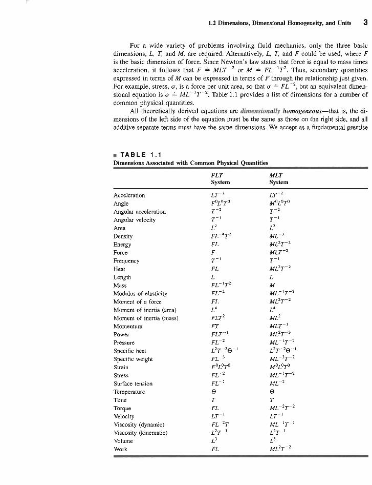
. Table' 1.1 provides a list of dimensions for a number of common physical quantities.

All theoretically derived equations are dimensionally homogeneous-that is, the di­mensions of the left side of the equation must be the same as those on the right side, and all additive separate terms must have the same dimensions. We accept as a fundamental premise

• TABLE 1.1 Dimensions Associated with Common Physical Quantities

FLT MLT System System

Acceleration LT-2 LT- 2

Angle FOLoTo MOLora

Angular acceleration T- 2 T- 2

Angular velocity T- 1 T- 1

Area L2 L2

Density FL- 4T 2 ML- 3

Energy FL ML2T- 2

Force F MLT-2

Frequency T- 1 T- 1

Heat FL ML2T- 2

Length L L

Mass FL- 1T 2 M

Modulus of elasticity FL- 2 ML- tT- 2

Moment of a force FL ML2T- 2

Moment of inertia (area) L4 L4

Moment of inertia (mass) FLT2 ML2

Momentum FT MLT- t

Power FLT- 1 ML2T- 3

Pressure FL- 2 ML- 1T- 2

Specific heat L2T- 2e- t L2T- 2e- t

Specific weight FL- 3 ML- 2T- 2

Strain FOLoTo MOLoTo

Stress FL- 2 ML- 1T- 2

Surface tension FL- 1 ML- 2

Temperature e e Time T T Torque FL ML-2T- 2

Velocity LT- 1 LT- t

Viscosity (dynamic) FL-2T ML-1T- 1

Viscosity (kinematic) L2T- 1 L2T- t

Volume L3 L3

Work FL ML2T- 2

4 Chapter 1 • Introduction

that all equations describing physical phenomena must be dimensionally homogeneous. For example, the equation for the velocity, V, of a uniformly accelerated body is

v = Vo + at (1.1)

where Vois the initial velocity, a the acceleration, and t the time interval. In terms of dimen­sions the equation is

LT- 1 == LT- 1 + LT- 1

and thus Eq. 1.1 is dimensionally homogeneous. Some equations that are known to be valid contain constants having dimensions. The

equation for the distance, d, traveled by a freely falling body can be written as

d = 16.1t2 (1.2)

and a check of the dimensions reveals that the constant must have the dimensions of LT-2

if the equation is to be dimensionally homogeneous. Actually, Eq. 1.2 is a special form of the well-known equation from physics for freely falling bodies,

2t d = T (1.3)

in which g is the acceleration of gravity. Equation 1.3 is dimensionally homogeneous and valid in any system of units. For g = 32.2 ft/s 2 the equation reduces to Eq. 1.2, and thus Eq. 1.2 is valid only for the system of units using feet and seconds. Equations that are restricted to a particular system of units can be denoted as restricted homogeneous equa­tions, as opposed to equations valid in any system of units, which are general homogeneous equations. The concept of dimensions also forms the basis for the powerful tool of dimens­ional analysis, which is considered in detail in Chapter 7.

Note to the users of this text. All of the examples in the text use a consistent problem­solving methodology which is similar to that in other engineering courses such as statics. Each example highlights the key elements of analysis: Given, Find, Solution, and Comment.

The Given and Find are steps that ensure the user understands what is being asked in the problem and explicitly list the items provided to help solve the problem.

The Solution step is where the equations needed to solve the problem are formulated and the problem is actually solved. In this step, there are typically several other tasks that help to set up the solution and are required to solve the problem. The first is a drawing of the problem; where appropriate, it is always helpful to draw a sketch of the problem. Here the relevant geometry and coordinate system to be used as well as features such as control volumes, forces and pressures, velocities and mass flow rates are included. This helps in gaining a visual understanding of the problem. Making appropriate assumptions to solve the problem is the second task. In a realistic engineering problem-solving environment, the necessary assumptions are developed as an integral part of the solution process. Assump­tions can provide appropriate simplifications or offer useful constraints, both of which can help in solving the problem. Throughout the examples in this text, the necessary assump­tions are embedded within the Solution step, as they are in solving a real-world problem. This provides a realistic problem-solving experience.

The final element in the methodology is the Comment. For the examples in the text, this section is used to provide further insight into the problem or the solution. It can also be a point in the analysis at which certain questions are posed. For example: Is the answer reasonable, and does it make physical sense? Are the final units correct? If a certain param­eter were changed, how would the answer change? Adopting the above type of methodol­ogy will aid in the development of problem-solving skills for fluid mechanics, as well as other engineering disciplines.

------- -------- -------

5 1.2 Dimensions, Dimensional Homogeneity, and Units

EXAMPLE 1.1 Restricted and General Homogeneous Equations

GIVEN A commonly used equation for determining the volume rate of flow, Q. of a liquid through an orifice located in the side of a tank as shown in Fig. El.! is

Q = 0.61 Av2ih where A is the area of the orifice, g is the acceleration of grav­ity, and h is the height of the liquid above the orifice.

FIND Investigate the dimensional homogeneity of this formula.

-

• FIGURE E1.1 SOLUTION _

The dimensions of the various terms in the equation are A quick check of the dimensions reveals that

Q = volume/time == L3T- 1 L3T- 1 == (4.90)(L512

)

L2A = area == and, therefore, the equation expressed as Eq. I can only be

g = acceleration of gravity == LT-2 dimensionally correct if the number, 4.90, has the dimensions

h = height == L of L1/2T -I. Whenever a number appearing in an equation or formula has dimensions, it means that the specific value ofThese terms, when substituted into the equation, yield the di­the number will depend on the system of units used. Thus, for mensional form the case being considered with feet and seconds used as units, the number 4.90 has units of ft l/2/s. Equation I will only give the correct value for Q (in ft3/s) when A is ex­pressed in square feet and h in feet. Thus, Eq. 1 is a restricted homogeneous equation, whereas the original equation is a

It is clear from this result that the equation is dimensionally ho­ general homogeneous equation that would be valid for any mogeneous (both sides of the formula have the same dimensions consistent system of units. A quick check of the dimensions of L3T- 1

), and the numbers (0.61 and V2) are dimensionless. of the various terms in an equation is a useful practice and will often be helpful in eliminating errors-that is, as noted COMMENT If we were going to use this relationship re­previously, all physically meaningful equations must be di­

peatedly, we might be tempted to simplify it by replacing g mensionally homogeneous. We have briefly alluded to units

with its standard value of 32.2 ft/s2 and rewriting the formula as in this example, and this important topic will be considered

Q = 4.90AYh (1) in more detail in the next section.

or

1.2.1 Systems of Units

In addition to the qualitative description of the various quantities of interest, it is generally nec­essary to have a quantitative measure of any given quantity. For example, if we measure the width of this page in the book and say that it is 10 units wide, the statement has no meaning un­til the unit of length is defined. If we indicate that the unit of length is a meter, and define the meter as some standard length, a unit system for length has been established (and a numerical value can be given to the page width). In addition to length, a unit must be established for each of the remaining basic quantities (force, mass, time, and temperature). There are several sys­tems of units in use and we shall consider two systems that are commonly used in engineering.

British Gravitational (BG) System. In the BG system the unit of length is the foot (ft), the time unit is the second (s), the force unit is the pound (lb), and the temperature unit is the degree Fahrenheit (OF), or the absolute temperature unit is the degree Rankine CR), where

OR = OF + 459.67

6 Chapter 1 • Introduction

The mass unit, called the slug, is defined from Newton's second law (force mass X

acceleration) as

lIb = (1 slug)(l ft/s2)

This relationship indicates that a l-lb force acting on a mass of 1 slug will give the mass an acceleration of 1 ft/s2

•

The weight, 'W (which is the force due to gravity, g) of a mass, m, is given by the equation

'W = mg

and in BG units

'W (lb) = m (slugs) g (ft/s2)

Since the earth's standard gravity is taken as g = 32.174 ft/s2 (commonly approximated as 32.2 ft/s 2), it follows that a mass of 1 slug weighs 32.2 lb under standard gravity.

Flu ids in the New 5

How long is a foot? Today, in the United States, the common length unit is the foot, but throughout antiquity the unit used to measure length has quite a history. The first length units were based on the lengths of various body parts. One of the earliest units was the Egyptian cubit, first used around 3000 B.C. and defined as the length of the arm from elbow to extended fin­gertips. Other measures followed with the foot simply taken as the length of a man's foot. Since this length obviously varies from person to person it was often "standardized" by using the length of the current reigning royalty's foot. In 1791

a special French commission proposed that a new universal length unit called a meter (metre) be defined as the distance of one-quarter of the earth's meridian (north pole to the equa­tor) divided by 10 million. Although controversial, the meter was accepted in 1799 as the standard. With the development of advanced technology, the length of a meter was redefined in 1983 as the distance traveled by light in a vacuum during the time interval of 11299,792,458 s. The foot is now defined as 0.3048 meters. Our simple rulers and yardsticks indeed have an intriguing history.•

International System (SI). In 1960, the Eleventh General Conference on Weights and Measures, the international organization responsible for maintaining precise uniform standards of measurements, formally adopted the International System of Units as the inter­national standard. This system, commonly termed SI, has been adopted worldwide and is widely used (although certainly not exclusively) in the United States. It is expected that the long-term trend will be for all countries to accept SI as the accepted standard, and it is imperative that engineering students become familiar with this system. In SI the unit of length is the meter (m), the time unit is the second (s), the mass unit is the kilogram (kg), and the temperature unit is the kelvin (K). Note that there is no degree symbol used when expressing a temperature in kelvin units. The Kelvin temperature scale is an absolute scale and is related to the Celsius (centigrade) scale (0C) through the relationship

K = °C + 273.15

Although the Celsius scale is not in itself part of SI, it is common practice to specify tem­peratures in degrees Celsius when using SI units.

The force unit, called the newton (N), is defined from Newton's second law as

1 N = (lkg)(l m/s2)

Thus, a l-N force acting on a I-kg mass will give the mass an acceleration of 1 m/s2. Standard

gravity in SI is 9.807 m/s2 (commonly approximated as 9.81 m/s2) so that a I-kg mass weighs

9.81 N under standard gravity. Note that weight and mass are different, both qualitatively and

7 1.3 Analysis of Fluid Behavior

• TABLE 1.2 Conversion Factors from BG Units to SI Units

(See inside of back cover.)

• TABLE 1.3 Conversion Factors from SI Units to BG Units

(See inside of back cover.)

quantitatively! The unit of work in SI is the joule (1), which is the work done when the point of application of a I-N force is displaced through a l-m distance in the direction of the force. Thus,

1 J = IN· m

The unit of power is the watt (W) defined as a joule per second. Thus,

1 W = 1 J/s = 1 N . mls

Prefixes for forming multiples and fractions of SI units are commonly used. For exam­ple, the notation kN would be read as "kilonewtons" and stands for 103N. Similarly, mm would be read as "millimeters" and stands for 1O-3m. The centimeter is not an accepted unit of length in the SI system, and for most problems in fluid mechanics in which SI units are used, lengths will be expressed in millimeters or meters.

In this text we will use the BG system and SI for units. Approximately one-half the problems and examples are given in BG units and one-half in SI units. Tables 1.2 and 1.3 provide conversion factors for some quantities that are commonly encountered in fluid mechanics, and these tables are located on the inside of the back cover. Note that in these tables (and others) the numbers are expressed by using computer exponential notation. For example, the number 5.154 E + 2 is equivalent to 5.154 X 102 in scientific notation, and the number 2.832 E - 2 is equivalent to 2.832 X 10-2

. More extensive tables of conver­sion factors for a large variety of unit systems can be found in Appendix E.

Flu ids in the New s

Units and space travel A NASA spacecraft. the Mars Climate Errors in the maneuvering commands sent from earth caused Orbiter, was launched in December 1998 to study the Martian the Orbiter to sweep within 37 miles of the surface rather than geography and weather patterns. The spacecraft was slated to the intended 93 miles. The subsequent investigation revealed begin orbiting Mars on September 23, 1999. However, NASA that the errors were due to a simple mix-up in units. One team officials lost communication with the spacecraft early that controlling the Orbiter used SI units whereas another team day. and it is believed that the spacecraft broke apart or over­ used BG units. This costly experience illustrates the impor­heated because it came too close to the surface of Mars. tance of using a consistent system of units.•

1.3 Analysis of Fluid Behavior

The study of fluid mechanics involves the same fundamental laws you have encountered in physics and other mechanics courses. These laws include Newton's laws of motion, con­servation of mass, and the first and second laws of thermodynamics. Thus. there are strong similarities between the general approach to fluid mechanics and to rigid-body and deformable-body solid mechanics.

8 Chapter 1 • Introduction

The broad subject of fluid mechanics can be generally subdivided into fluid statics, in which the fluid is at rest, and fluid dynamics, in which the fluid is moving. In subse­quent chapters we will consider both of these areas in detail. Before we can proceed, how­ever, it will be necessary to define and discuss certain fluid properties that are intimately related to fluid behavior. In the following several sections, the properties that play an impor­tant role in the analysis of fluid behavior are considered.

1.4 Measures of Fluid Mass and Weight

1.4.1 Density

The density of a fluid, designated by the Greek symbol p (rho), is defined as its mass per unit volume. Density is typically used to characterize the mass of a fluid system. In the BG system, p has units of slugs/ft3 and in SI the units are kg/m3

.

The value of density can vary widely between different fluids, but for liquids, varia­tions in pressure and temperature generally have only a small effect on the value of p. The small change in the density of water with large variations in temperature is illustrated in Fig. 1.1. Tables 1.4 and 1.5 list values of density for several common liquids. The density of water at 60° F is 1.94 slugs/ft3 or 999 kg/m3

. The large difference between those two values illustrates the importance of paying attention to units! Unlike liquids, the density of a gas is strongly influenced by both pressure and temperature, and this difference is dis­cussed in the next section.

The specific volume, v, is the volume per unit mass and is therefore the reciprocal of the density-that is,

1 v=- (1.4)

P

This property is not commonly used in fluid mechanics but is used in thermodynamics.

1.4.2 Specific Weight

The specific weight of a fluid, designated by the Greek symbol 'Y (gamma), is defined as its weight per unit volume. Thus, specific weight is related to density through the equation

'Y = pg (1.5)

1000

990)

'"E Ob 980 -'" "­~ .~ 970 Q)

o

960)

950 o 10080604020

\ r--~

j' .......

\ ~@ 4°C P = 1000 kg/m3

i".... .......

~~ - -

I ,

'-....

Temperature, °C

• FIG U R E 1. 1 Density of water as a function of temperature.

9 I.S Ideal Gas Law

• TABLE 1.4 Approximate Physical Properties of Some Common Liquids (BG Units)

(See inside of front cover.)

• TABLE 1.5 Approximate Physical Properties of Some Common Liquids (SI Units)

(See inside of front cover.)

where g is the local acceleration of gravity. Just as density is used to characterize the mass of a fluid system, the specific weight is used to characterize the weight of the system. In the BG system, y has units of Ib/ft3 and in SI the units are N/m3

. Under conditions of stan­dard gravity (g = 32.174 ft/s2 = 9.807 rn/s2

), water at 60° F has a specific weight of 62.4 Ib/ft3

and 9.80 kN/m3. Tables 1.4 and 1.5 list values of specific weight for several common liquids

(based on standard gravity). More complete tables for water can be found in Appendix B (Tables B.l and B.2).

1.4.3 Specific Gravity

The specific gravity of a fluid, designated as SG, is defined as the ratio of the density of the fluid to the density of water at some specified temperature. Usually the specified tempera­ture is taken as 4° C (39.2° F), and at this temperature the density of water is 1.94 slugs/ft3

or 1000 kg/m 3. In equation form specific gravity is expressed as

SG = _.....:.P_­ (1.6)PH20@4°C

and since it is the ratio of densities, the value of SG does not depend on the system of units used. For example, the specific gravity of mercury at 20° Cis 13.55, and the density of mer­cury can thus be readily calculated in either BG or SI units through the use of Eq. 1.6 as

PHg = (13.55)( 1.94 slugs/ft3) = 26.3 slugs/ft3

or

PHg = (13.55)( 1000 kg/m3 ) = 13.6 X 103 kg/m3

It is clear that density, specific weight, and specific gravity are all interrelated, and from a knowledge of anyone of the three the others can be calculated.

1.5 Ideal Gas Law

Gases are highly compressible in comparison to liquids, with changes in gas density directly related to changes in pressure and temperature through the equation

p = pRT (1.7)

where p is the absolute pressure, P the density, T the absolute temperature, I and R is a gas constant. Equation 1.7 is commonly termed the perfect or ideal gas law, or the equation of

lWe will use T to represent temperature in thennodynamic relationships. although T is also used to denote the basic dimension of time.

12 Chapter 1 • Introduction

Since 8a = U 8t it follows that

8{3 = U 8t b

Note that in this case, 8{3 is a function not only of the force P (which governs U) but also of time. We consider the rate at which 8{3 is changing, and define the rate ofshearing strain, 'Y, as

. 8{3'Y = lim­

St->O 8t

which in this instance is equal to

. U du 'Y=-=­

b dy

A continuation of this experiment would reveal that as the shearing stress, T, is increased by increasing P (recall that T = PIA), the rate of shearing strain is increased in direct proportion-that is

TCX'Y

or

du T cx ­

dy

This result indicates that for common fluids, such as water, oil, gasoline, and air, the shearing stress and rate of shearing strain (velocity gradient) can be related with a relationship of the form

du T = J.L - (1.8)

dy

where the constant of proportionality is designated by the Greek symbol J.L (mu) and is called the absolute viscosity, dynamic viscosity, or simply the viscosity of the fluid. In accordance with Eq. 1.8, plots of T versus du/dy should be linear with the slope equal to the viscosity as illustrated in Fig. 1.3. The actual value of the viscosity depends on the particular fluid, and for a particular

V1.3 Capillary tube fluid the viscosity is also highly dependent on temperature as illustrated in Fig. 1.3 with the two viscometer curves for water. Fluids for which the shearing stress is linearly related to the rate of shearing

strain (also referred to as rate of angular deformation) are designated as Newtonianfluids. Fortu­nately, most common fluids, both liquids and gases, are Newtonian. A more general formulation ofEq. 1.8, which applies to more complex flows of Newtonian fluids, is given in Section 6.8.1.

Fluids for which the shearing stress is not linearly related to the rate of shearing strain VIA Non­ are designated as non-Newtonian fluids. It is beyond the scope of this book to consider the Newtonian behavior behavior of such fluids, and we will only be concerned with Newtonian fluids.

Flu ids in the New s A vital fluid In addition to air and water, another fluid that is essential for human life is blood. Blood is an unusual flui,d con­sisting of red blood cells that are disk-shaped, about 8 microns in diameter, suspended in plasma. As you would suspect, since blood is a suspension, its mechanical behavior is that of a non-Newtonian fluid. Its density is only slightly higher than that of water, but its typical apparent viscosity is signifi­cantly higher than that of water at the same temperature. It is difficult to measure the viscosity of blood since it is a non­Newtonian fluid and the viscosity is a function of the shear

rate. As the shear rate is increased from a low value, the ap­parent viscosity decreases and approaches asymptotically a constant value at high shear rates. The "asymptotic" value of the viscosity of normal blood is 3 to 4 times the viscosity of water. The viscosity of blood is not routinely measured like some biochemical properties such as cholesterol and triglyc­erides, but there is some evidence indicating that the viscosity of blood may playa role in the development of cardiovascular disease. If this proves to be true, viscosity could become a stan­dard variable to be routinely measured. (See Problem 1.24.) •

1.6 Viscosity 13

• FIG U R E 1. 3 Linear varia­tion of shearing stress with rate of

Rate of shearing strain, '!g shearing strain for common fluids.

From Eq. 1.8 it can be readily deduced that the dimensions of viscosity are FTL-2. Thus, in BG units viscosity is given as Ib's/ft2 and in SI units as N·s!m2

. Values of viscosity for sev­eral common liquids and gases are listed in Tables 1.4 through 1.7. A quick glance at these tables reveals the wide variation in viscosity among fluids. Viscosity is only mildly dependent on pressure, and the effect of pressure is usually neglected. However, as mentioned previously, and as illustrated in Appendix B (Figs. B.I and B.2), viscosity is very sensitive to temperature.

Quite often viscosity appears in fluid flow problems combined with the density in the form

J.L v=­P

This ratio is called the kinematic viscosity and is denoted with the Greek symbol (nu).J)

The dimensions of kinematic viscosity are L2/T, and the BG units are ft2/S and SI units are m2/s. Values of kinematic viscosity for some common liquids and gases are given in Tables 1.4 through 1.7. More extensive tables giving both the dynamic and kinematic viscosities for water and air can be found in Appendix B (Tables B.l through B.4), and graphs showing the variation in both dynamic and kinematic viscosity with temperature for a variety of flu­ids are also provided in Appendix B (Figs. B.l and B.2).

Although in this text we are primarily using BG and SI units, dynamic viscosity is often expressed in the metric CGS (centimeter-gram-second) system with units of dyne·s/cm2. This combination is called a poise, abbreviated P. In the CGS system, kine­matic viscosity has units of cm2/s, and this combination is called a stoke, abbreviated St.

EXAMPLE 1.3 Viscosity and Dimensionless Quantities

GIVEN A dimensionless combination of variables that is flows through a 25-mm-diameter pipe with a velocity of important in the study of viscous flow through pipes is 2.6 mls.

called the Reynolds number, Re, defined as pVDIp. where FIND Determine the value of the Reynolds number using p is the fluid density, V the mean fluid velocity, D the pipe

(a) 51 units and diameter, and p. the fluid viscosity. A Newtonian fluid hav­ing a viscosity of 0.38 N's/m2 and a specific gravity of 0.91 (b) BG units.

14 Chapter 1 • Introduction

SOLUTION

(a) The fluid density is calculated from the specific gravity as

p = SGPH,0@4'c=0.91 (IOOOkg/m3) = 91Okg/m3

and from the definition of the Reynolds number

pVD (910 kg/m3)(2.6 m/s)(25 mm)(10-3 m/mm)Re=­

JL 0.38 N's/m2

= l56(kg'mls2)/N

However, since I N = I kg'm/S2 it follows that the Reynolds number is unitJess (dimensionless)-that is,

Re = 156 (ADs)

COMMENT The value of any dimensionless quantity does not depend on the system of units used if all variables that make up the quantity are expressed in a consistent set of units. To check this we will calculate the Reynolds number using BG units.

(b) We first convert all the SI values of the variables appear­ing in the Reynolds number to BG values by using the conver­sion factors from Table 1.3. Thus,

_

p = (910 kg/m3 )(1.940 X 10-3) = 1.77 slugs/ft3

V = (2.6 m/s)(3.281) = 8.53 ftls

D = (0.025 m)(3.281) = 8.20 X 10-2 ft

JL = (0.38 N·s/m2)(2.089 X 10-2) = 7.94 X 1O-3 Ib's/ft2

and the value of the Reynolds number is

(1.77 slugs/ft3)(8.53 ftls)(8.20 X 10-2 ft)Re = -'-----'--'--'-----'--------'­

7.94 X 1O-3 Ib's/ft2

= 156(slug'ftls2)/lb = 156 (ADS)

since lIb = I slug·ftls2.

COMMENT The values from part (a) and part (b) are the same, as expected. Dimensionless quantities play an important role in fluid mechanics, and the significance of the Reynolds number, as well as other important dimensionless combina­tions, will be discussed in detail in Chapter 7. It should be noted that in the Reynolds number it is actually the ratio JLlp that is important, and this is the property that we have defined as the kinematic viscosity.

EXAMPLE 1.4 Newtonian Fluid Shear Stress

GIVEN The velocity distribution for the flow of a Newton­ian fluid between two wide, parallel plates (see Fig. E1.4) is given by the equation

u = 3;[ I-GJJ where V is the mean velocity. The fluid has a viscosity of 0.04lb·s/ft2

. Also, V = 2 ftls and h = 0.2 in.

SO LUTION ---.,

For this type of parallel flow the shearing stress is obtained from Eq. 1.8.

du (1)

T = JL dy

FIND Determine

(a) the shearing stress acting on the bottom wall and

(b) the shearing stress acting on a plane parallel to the walls and passing through the centerline (midplane).

• FIGURE E1.4

Thus, if the velocity distribution, u = u(y), is known, the shear­and therefore the shearing stress is

ing stress can be determined at all points by evaluating the ve­locity gradient, du/dy. For the distribution given 3V) (0.04 Ib's/ft2)(3)(2 ftls)

Tbottom wall = JL ( h = (0.2 in.)(1 ftll2 in.)du = _ 3Vy

dy h2 (2) = 14.4 Ib/ft2 (in direction of flow) (ADS)

(a) Along the bottom wall y = -h so that (from Eq. 2) COMMENT This stress creates a drag on the wall. Since the velocity distribution is symmetrical, the shearing stress along du 3V the upper wall would have the same magnitude and direction.

dy h

-------

(b) Along the midplane where y = 0, it follows from Eq. 2 that

du = 0 dy

and thus the shearing stress is

(Ans)Tmidplane = 0

1.7 Compressibility of Fluids

1.7 Compressibility of Fluids 15

COMMENT From Eq. 2 we see that the velocity gradient (and therefore the shearing stress) varies linearly with y and in this particular example varies from 0 at the center of the channel to 14.4 Ib/ft2 at the walls. For the more general case the actual variation will, of course, depend on the nature of the velocity distribution.

p

p +dp

¥-dV

1.7.1 Bulk Modulus

An important question to answer when considering the behavior of a particular fluid is how easlly can the volume (and thus the density) of a given mass of the fluid be changed when there is a change in pressure? That is, how compressible is the fluid? A property that is commonly used to characterize compressibility is the bulk modulus, Ev , defined as

dp (1.9)Ev = - dV/v

where dp is the differential change in pressure needed to create a differential change in volume, dV, of a volume V, as shown by the figure in the margin. The negative sign is included since an increase in pressure will cause a decrease in volume. Because a decrease in volume of a given mass, m = pV, will result in an increase in density, Eq. 1.9 can also be expressed as

dpE =- (1.10)

v dp/p

The bulk modulus (also referred to as the bulk modulus of elasticity) has dimensions of pressure, FL-2. In BG units values for Ev are usually given as lb/in? (psi) and in SI units as N/m2 (Pa). Large values for the bulk modulus indicate that the fluid is relatively incom­pressible-that is, it takes a large pressure change to create a small change in volume. As expected, values of Ev for common liquids are large (see Tables 1.4 and 1.5).

Since such large pressures are required to effect a change in volume, we conclude that liquids can be considered as incompressible for most practical engineering applications. As liquids are compressed the bulk modulus increases, but the bulk modulus near atmos­pheric pressure is usually the one of interest. The use of bulk modulus as a property describ­ing compressibility is most prevalent when dealing with liquids, although the bulk modu­lus can also be determined for gases.

Flu ids in the New s This water jet is a blast Usually liquids can be treated as in­ or 3000 to 4000 atmospheres), the water is compressed (i.e., the compressible fluids. However, in some applications the comp­ volume reduced) by about 10 to 15%. When a fast-opening ressibility of a liquid can playa key role in the operation of a de­ valve within the pressure vessel is opened, the water expands vice. For example, a water pulse generator using compressed and produces a jet of water that upon impact with the target ma­water has been developed for use in mining operations. It can terial produces an effect similar to the explosive force from con­fracture rock by producing an effect comparable to a conven­ ventional explosives. Mining with the water jet can eliminate tional explosive such as gunpowder. The device uses the energy various hazards that arise with the use of conventional chemical stored in a water-filled accumulator to generate an ultrahigh­ explosives such as those associated with the storage and use of pressure water pulse ejected through a 10- to 25-mm-diameter explosives and the generation of toxic gas by-products that re­discharge valve. At the ultrahigh pressures used (300 to 400 MPa, quire extensive ventilation. (See Problem 1.43.) •

16 Chapter 1 • Introduction

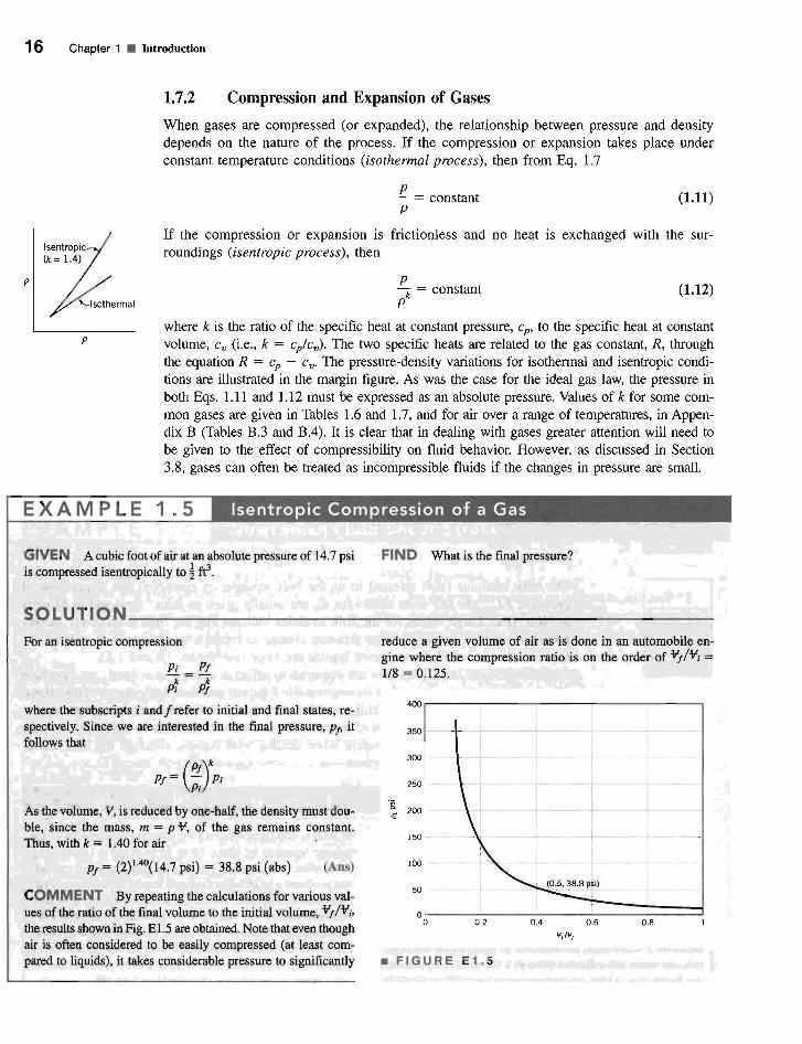
1.7.2 Compression and Expansion of Gases

When gases are compressed (or expanded), the relationship between pressure and density depends on the nature of the process. If the compression or expansion takes place under constant temperature conditions (isothermal process), then from Eq. 1.7

p - = p

constant (1.11)

If the compression or expansion is frictionless and roundings (isentropic process), then

no heat is exchanged with the sur­

Pk p

= constant (1.12)

p where k is the ratio of the specific heat at constant pressure, cp, to the specific heat at constant volume, Cv (i.e., k = cp/cv ). The two specific heats are related to the gas constant, R, through the equation R = cp - Cv . The pressure-density variations for isothermal and isentropic condi­tions are illustrated in the margin figure. As was the case for the ideal gas law, the pressure in both Eqs. 1.11 and 1.12 must be expressed as an absolute pressure. Values of k for some com­mon gases are given in Tables 1.6 and 1.7, and for air over a range of temperatures, in Appen­dix B (Tables B.3 and B.4). It is clear that in dealing with gases greater attention will need to be given to the effect of compressibility on fluid behavior. However, as discussed in Section 3.8, gases can often be treated as incompressible fluids if the changes in pressure are small.

p

EXAMPLE 1 .5 Isentropic Compression of a Gas

GIVEN A cubic foot of air at an absolute pressure of 14.7 psi is compressed isentropically to 4fe.

SOLUTION

For an isentropic compression

Pi Pt P~ = pj

where the subscripts i and f refer to initial and final states, re­spectively. Since we are interested in the final pressure, Pt' it follows that

Pt)kPt = ( -; Pi

As the volume, V, is reduced by one-half, the density must dou­ble, since the mass, m = P V, of the gas remains constant. Thus, with k = 1.40 for air

Pt = (2)1.40(14.7 psi) = 38.8 psi (abs) (Ans)

COMMENT By repeating the calculations for various val­ues ofthe ratio of the final volume to the initial volume, Vf/V;, the results shown in Fig. El.5 are obtained. Note that even though air is often considered to be easily compressed (at least com­pared to liquids), it takes considerable pressure to significantly

FIND What is the final pressure?

_

reduce a given volume of air as is done in an automobile en­gine where the compression ratio is on the order of Vt/Vi =

1/8 = 0.125.

400

350

300

250

.~ 200 "­

150

100

50

0 0 0.2 0.4 0.6 0.8

1',"",

• FIGURE E1.5

1.7 Compressibility of Fluids 17

6000

water

4000 -

~

'" 2000 -

air

0 0 100

T. deg F 200

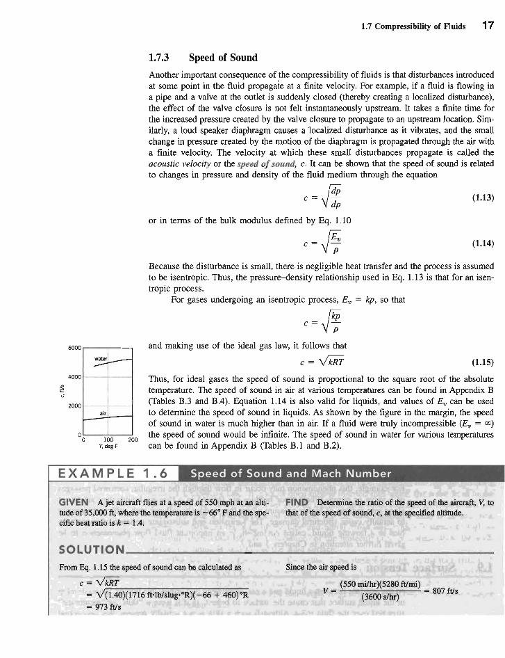
1.7.3 Speed of Sound

Another important consequence of the compressibility of fluids is that disturbances introduced at some point in the fluid propagate at a finite velocity. For example, if a fluid is flowing in a pipe and a valve at the outlet is suddenly closed (thereby creating a localized disturbance), the effect of the valve closure is not felt instantaneously upstream. It takes a finite time for the increased pressure created by the valve closure to propagate to an upstream location. Sim­ilarly, a loud speaker diaphragm causes a localized disturbance as it vibrates, and the small change in pressure created by the motion of the diaphragm is propagated through the air with a finite velocity. The velocity at which these small disturbances propagate is called the acoustic velocity or the speed of sound, c. It can be shown that the speed of sound is related to changes in pressure and density of the fluid medium through the equation

C -­ fdPddP p\j d; (1.13)

or in terms of the bulk modulus defined by Eq. 1.10

c=1j (1.14)

Because the disturbance is small, there is negligible heat transfer and the process is assumed to be isentropic. Thus, the pressure-density relationship used in Eq. 1.13 is that for an isen­tropic process.

For gases undergoing an isentropic process, Ev = kp, so that

c=J¥ and making use of the ideal gas law, it follows that

c = v'idiT (1.15)

Thus, for ideal gases the speed of sound is proportional to the square root of the absolute temperature. The speed of sound in air at various temperatures can be found in Appendix B (Tables B.3 and B.4). Equation 1.14 is also valid for liquids, and values of Ev can be used to determine the speed of sound in liquids. As shown by the figure in the margin, the speed of sound in water is much higher than in air. If a fluid were truly incompressible (Ev = 00) the speed of sound would be infinite. The speed of sound in water for various temperatures can be found in Appendix B (Tables B.I and B.2).

1.6 Speed of Sound and Mach NumberEXAMPLE

GIVEN A jet aircraft flies at a speed of 550 mph at an alti­ FIND Determine the ratio of the speed of the aircraft, V, to tude of 35,000 ft, where the temperature is -66° F and the spe­ that of the speed of sound, c, at the specified altitude. cific heat ratio is k = 1.4.

SOLUTION

From Eq. 1.15 the speed of sound can be calculated as

C = VkRT = yr-(1-.4-0-)(-17-l6-f-t.-lb-/s-lu-g-.oR-)-(--6-6-+-46-0-)o-R

= 973 ftls

_

Since the air speed is

(550 mi/hr)(5280 ftlmi) V = (3600 s/hr) = 807 ftls

I

18 Chapter 1 • Introduction

the ratio is

V 807 ftis = 0.829 (ADS)~ = 973 ftis

COMMENT This ratio is called the Mach number, Ma. If Ma < 1.0 the aircraft is flying at subsonic speeds, whereas for Ma > 1.0 it is flying at supersonic speeds. The Mach number is an important dimensionless parameter used in the study of the flow of gases at high speeds and will be further discussed in Chapters 7 and 9.

By repeating the calculations for different temperatures, the results shown in Fig. E1.6 are obtained. Because the speed of sound increases with increasing temperature, for a constant airplane speed, the Mach number decreases as the temperature increases.

1.8 Vapor Pressure

0.9 I

0.8

:;:v

" 0.7 ::<'"

0.6

0.5 I I

-100 -50 50 100

• FIGURE E1.6

~ Liquid

•-

t Vapor,P.

Liquid

It is a common observation that liquids such as water and gasoline will evaporate if they are simply placed in a container open to the atmosphere. Evaporation takes place because some liquid molecules at the surface have sufficient momentum to overcome the intermol­ecular cohesive forces and escape into the atmosphere. As shown in the figure in the margin, if the lid on a completely liquid-filled, closed container is raised (without letting any air in), a pressure will develop in the space as a result of the vapor that is formed by the escaping molecules. When an equilibrium condition is reached so that the number of molecules leav­ing the surface is equal to the number entering, the vapor is said to be saturated and the pressure the vapor exerts on the liquid surface is termed the vapor pressure, Pv.

Since the development of a vapor pressure is closely associated with molecular activ­ity, the value of vapor pressure for a particular liquid depends on temperature. Values of vapor pressure for water at various temperatures can be found in Appendix B (Tables B.l and B.2), and the values of vapor pressure for several common liquids at room tempera­tures are given in Tables 1.4 and 1.5. Boiling, which is the formation of vapor bubbles within a fluid mass, is initiated when the absolute pressure in the fluid reaches the vapor pressure.

An important reason for our interest in vapor pressure and boiling lies in the com­mon observation that in flowing fluids it is possible to develop very low pressure due to the fluid motion, and if the pressure is lowered to the vapor pressure, boiling will occur. For example, this phenomenon may occur in flow through the irregular, narrowed passages of a valve or pump. When vapor bubbles are formed in a flowing liquid, they are swept along into regions of higher pressure where they suddenly collapse with sufficient intensity to actually cause structur.al damage. The formation and subsequent collapse of vapor bub­bles in a flowing liquid, called cavitation, is an important fluid flow phenomenon to be given further attention in Chapters 3 and 7.

1.9 Surface Tension

At the interface between a liquid and a gas, or between two immiscible liquids, forces develop in the liquid surface that cause the surface to behave as if it were a "skin" or "membrane" stretched over the fluid mass. Although such a skin is not actually present, this conceptual

V1.5 Floating razor I)lades

1.9 Surface Tension 19

analogy allows us to explain several commonly observed phenomena. For example, a steel needle or razor blade will float on water if placed gently on the surface because the ten­sion developed in the hypothetical skin supports these objects. Small droplets of mercury will form into spheres when placed on a smooth surface because the cohesive forces in the surface tend to hold all the molecules together in a compact shape. Similarly, discrete water droplets will form when placed on a newly waxed surface.

These various types of surface phenomena are due to the unbalanced cohesive forces acting on the liquid molecules at the fluid surface. Molecules in the interior of the fluid mass are surrounded by molecules that are attracted to each other equally. However, mole­cules along the surface are subjected to a net force toward the interior. The apparent phys­ical consequence of this unbalanced force along the surface is to create the hypothetical skin or membrane. A tensile force may be considered to be acting in the plane of the sur­face along any line in the surface. The intensity of the molecular attraction per unit length along any line in the surface is called the surface tension and is designated by the Greek symbol cr (sigma). Surface tension is a property of the liquid and depends on temperature as well as the other fluid it is in contact with at the interface. The dimensions of surface tension are FL -1 with BG units of Ib/ft and SI units of N/m. Values of surface tension for some common liquids (in contact with air) are given in Tables 104 and 1.5 and in Appen­dix B (Tables B.l and B.2) for water at various temperatures. The value of the surface ten­sion decreases as the temperature increases.

Flu ids in the New 5

Walking on water Water striders are insects commonly video to examine in detail the movement of the water strid­found on ponds, rivers, and lakes that appear to "walk" on ers. They found that each stroke of the insect's legs creates water. A typical length of a water strider is about 0.4 in., and dimples on the surface with underwater swirling vortices they can cover 100 body lengths in one second. It has long sufficient to propel it forward. It is the rearward motion of been recognized that it is surface tension that keeps the wa­ the vortices that propels the water strider forward. To further ter strider from sinking below the surface. What has been substantiate their explanation the MIT team built a working puzzling is how they propel themselves at such a high model of a water strider, called Robostrider, which creates speed. They can't pierce the water surface or they would surface ripples and underwater vortices as it moves across a sink. A team of mathematicians and engineers from the water surface. Waterborne creatures, such as the water Massachusetts Institute of Technology (MIT) applied con­ strider, provide an interesting world dominated by surface ventional flow visualization techniques and high-speed tension. (See Problem 1.49.) •

Among common phenomena associated with surface tension is the rise (or fall) of a liquid in a capillary tube. If a small open tube is inserted into water, the water level in the tube will rise above the water level outside the tube as is illustrated in Fig. lAa. In this sit­uation we have a liquid-gas-solid interface. For the case illustrated there is an attraction (adhesion) between the wall of the tube and liquid molecules, which is strong enough to overcome the mutual attraction (cohesion) of the molecules and pull them up to the wall. Hence, the liquid is said to wet the solid surface.

The height, h, is governed by the value of the surface tension, cr, the tube radius, R, the specific weight of the liquid, y, and the angle of contact, e, between the fluid and tube. From the free-body diagram of Fig. lAb we see that the vertical force due to the surface tension is equal to 2'rrRcr cos e and the weight is 'Y'TrR2h and these two forces must balance for equilibrium. Thus,

20 Chapter 1 • Introduction

~ 21rRu

h~~,¥' -.l.

-+I 2R I- ­(a) (b) (c)

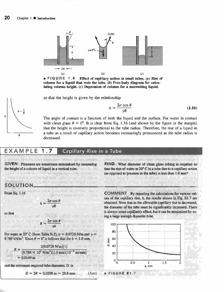
• FIG U R E 1. 4 Effect of capillary action in small tubes. (a) Rise of column for a liquid that wets the tube. (b) Free-body diagram for calcu­lating column height. (c) Depression of column for a nonwetting liquid.

so that the height is given by the relationship

2a cos (Jh=--­(1.16)

yR h

The angle of contact is a function of both the liquid and the surface. For water in contact with clean glass (J = 0°. It is clear from Eq. 1.16 (and shown by the figure in the margin) that the height is inversely proportional to the tube radius. Therefore, the rise of a liquid in a tube as a result of capillary action becomes increasingly pronounced as the tube radius is decreased.

EXAMPLE 1.7 Capillary Rise in a Tube

GIVEN Pressures are sometimes determined by measuring FIND What diameter of clean glass tubing is required so the height of a column of liquid in a vertical tube. that the rise of water at 20° C in a tube due to a capillary action

(as opposed to pressure in the tube) is less than 1.0 mm?

SOLUTION _

From Eq. 1.16 COMMENT By repeating the calculations for various val­ues of the capillary rise, h, the results shown in Fig. E1.7 are

2a cos (Jh=--- obtained. Note that as the allowable capillary rise is decreased,

'YR the diameter of the tube must be significantly increased. There is always some capillarity effect, but it can be minimized by us­so that ing a large enough diameter tube.

R = 2acos (J 100iii

'Yh 80

For water at 20° C (from Table B.2), U' = 0.0728 N/m and 'Y = 9.789 kN/m3

. Since (J "" 0° it follows that for h = 1.0 mm, E 60 E c::l 402(0.0728 N/m)(l)

R = -------:--'----,-----'------=-­(9.789 X 103 N/m3)(1.0 mm)(10-3 mlmm) 20 I I

= 0.0149 m 00 0.5

and the minimum required tube diameter, D, is

R

1 1.5 2 h, mm

D = 2R = 0.0298 m = 29.8 mm (Ans) • FIGURE E1.7

1.10 Chapter Summary and Study Guide 21

If adhesion of molecules to the solid surface is weak compared to the cohesion between molecules, the liquid will not wet the surface and the level in a tube placed in a nonwetting liquid will actually be depressed, as shown in Fig. lAc. Mercury is a good example of a nonwetting liquid when it is in contact with a glass tube. For nonwetting liquids the angle of contact is greater than 90°, and for mercury in contact with clean glass () = 130°.

Surface tension effects play a role in many mechanics problems, including the move­ment of liquids through soil and other porous media, flow of thin films, formation of drops and bubbles, and the breakup of liquid jets. Surface phenomena associated with liquid-gas, liquid-liquid, liquid-gas-solid interfaces are exceedingly complex, and a more detailed and rigorous discussion of them is beyond the scope of this text. Fortunately, in many fluid mechanics problems, surface phenomena, as characterized by surface tension, are not impor­tant, as inertial, gravitational, and viscous forces are much more dominant.

Flu ids in the New s Spreading of oil spills. With the large traffic in oil tankers ing the size of the spill, wind speed and direction, and the there is great interest in the prevention of and response to oil physical properties of the oil. These properties include spills. As evidenced by the famous Exxon Valdez oil spill in surface tension, specific gravity, and viscosity. The higher Prince William Sound in 1989, oil spills can create disastrous the surface tension the more likely a spill will remain in environmental problems. It is not surprising that much atten­ place. Since the specific gravity of oil is less than one it tion is given to the rate at which an oil spill spreads. When floats on top of the water, but the specific gravity of an oil spilled, most oils tend to spread horizontally into a smooth can increase if the lighter substances within the oil evapo­and slippery surface, called a slick. There are many factors rate. The higher the viscosity of the oil the greater the ten­which influence the ability of an oil slick to spread, includ- dency to stay in one place.•

1.10 Chapter Summary and Study Guide

fluid units basic dimensions dimensionally

homogeneous density specific weight specific gravity ideal gas law absolute pressure gage pressure no-slip condition absolute viscosity Newtonian fluid kinematic viscosity bulk modulus speed of sound vapor pressure surface tension

This introductory chapter discussed several fundamental aspects of fluid mechanics. Meth­ods for describing fluid characteristics both quantitatively and qualitatively are consid­ered. For a quantitative description, units are required, and in this text, two system of units are used: the British Gravitational (BG) System (pounds, slugs, feet, and seconds) and the International (SI) System (newtons, kilograms, meters, and seconds). For the qual­itative description the concept of dimensions is introduced in which basic dimensions such as length, L, time, T, and mass, M, are used to provide a description of various quanti­ties of interest. The use of dimensions is helpful in checking the generality of equations, as well as serving as the basis for the powerful tool of dimensional analysis discussed in detail in Chapter 7.

Various important fluid properties are defined, including fluid density, specific weight, specific gravity, viscosity, bulk modulus, speed of sound, vapor pressure, and surface ten­sion. The ideal gas law is introduced to relate pressure, temperature, and density in com­mon gases, along with a brief discussion of the compression and expansion of gases. The distinction between absolute and gage pressure is introduced, and this important idea is explored more fully in Chapter 2.

The following checklist provides a study guide for this chapter. When your study of the entire chapter and end-of-chapter exercises has been completed, you should be able to

• write out meanings of the terms listed here in the margin and understand each of the related concepts. These terms are particularly important and are set in color and bold type in the text.

• determine the dimensions of common physical quantities.

22 Chapter 1 • Introduction

• determine whether an equation is a general or restricted homogeneous equation.

• use both BG and SI systems of units.

• calculate the density, specific weight, or specific gravity of a fluid from a knowledge of any two of the three.

• calculate the density, pressure, or temperature of an ideal gas (with a given gas con­stant) from a knowledge of any two of the three.

• relate the pressure and density of a gas as it is compressed or expanded using Eqs. 1.11 and 1.12.

• use the concept of viscosity to calculate the shearing stress in simple fluid flows.

• calculate the speed of sound in fluids using Eq. 1.14 for liquids and Eq. 1.15 for gases.

• determine whether boiling or cavitation will occur in a liquid using the concept of vapor pressure.

• use the concept of surface tension to solve simple problems involving liquid-gas or liquid-solid-gas interfaces.

Review Problems

Go to Appendix F for a set of review problems with answers. Detailed solutions can be found in Student Solution Manual for a Brief Introduction to Fluid Mechanics. by Young et al. (© 2006 John Wiley and Sons, Inc.).

Problems

Note: Unless specific values of required fluid properties are given in the statement of the problem, use the values found in the tables on the inside of the front cover. Problems designated with an (*) are intended to be solved with the aid of a programmable calculator or a computer. Problems designated with a (t) are "open-ended" problems and require critical thinking in that to work them one must make various assumptions and provide the necessary data. There is not a unique answer to these problems.

Answers to the even-numbered problems are listed at the end of the book. Access to the videos that accompany problems can be obtained through the book's web site, www.wiley.com/ college/you.ng. The lab-type problems and FE problems can also be accessed on this web site.

Section 1.2 Dimensions, Dimensional Homogeneity, and Units 1.1 Verify the dimensions, in both the FLT and MLT sys­tems, of the following quantities, which appear in Table 1.1: (a) angular velocity, (b) energy, (c) moment of inertia (area), (d) power, and (e) pressure.

1.2 Determine the dimensions, in both the FLT system and MLT system, for (a) the product of force times volume, (b) the product of pressure times mass divided by area, and (c) moment of a force divided by velocity.

1.3 If V is a velocity, f a length, and v a fluid property hav­ing dimensions of L2T -I, which of the following combinations are dimensionless: (a) vev, (b) VeJv, (c) V 2v, (d) Vlfv?

1.4 Dimensionless combinations of quantities (commonly called dimensionless parameters) play an important role in fluid

mechanics. Make up five possible dimensionless parameters by using combinations of some of the quantities listed in Table 1.1.

1.5 The volume rate of flow, Q, through a pipe containing a slowly moving liquid is given by the equation

nR4 t:.pQ=g;e

where R is the pipe radius, t:.p the pressure drop along the pipe, p, a fluid property called viscosity (FL-21j, and f the length of pipe. What are the dimensions of the constant 71/8? Would you classify this equation as a general homogeneous equation? Explain.

1.6 The pressure difference, t:.p, across a partial blockage in an artery (called a stenosis) is approximated by the equation

p,V (Ao )2 2 t:.p = K v [) + Ku ~ - I pV

where V is the blood velocity, p, the blood viscosity (FL -2T), P the blood density (ML -3), D the artery diameter, Ao the area of the unobstructed artery, and A 1 the area of the stenosis. Determine the dimensions of the constants Kv and Ku- Would this equation be valid in any system of units?

1.7 According to information found in an old hydraulics book, the energy loss per unit weight of fluid flowing through a nozzle connected to a hose can be estimated by the formula

h = (0.04 to 0.09)(D/d)4V2/2g

where h is the energy loss per unit weight, D the hose diameter, d the nozzle tip diameter, V the fluid velocity in the hose, and g